
Welcome message from author
This document is posted to help you gain knowledge. Please leave a comment to let me know what you think about it! Share it to your friends and learn new things together.
Transcript

Power Electronics and Power Systems
For further volumes:http://www.springer.com/series/6403

Slobodan N. Vukosavic
Electrical Machines
Slobodan N. VukosavicDept. of Electrical EngineeringUniversity of BelgradeBelgrade, Serbia
ISBN 978-1-4614-0399-9 ISBN 978-1-4614-0400-2 (eBook)DOI 10.1007/978-1-4614-0400-2Springer New York Heidelberg Dordrecht London
Library of Congress Control Number: 2012944981
# Springer Science+Business Media New York 2013This work is subject to copyright. All rights are reserved by the Publisher, whether the whole or partof the material is concerned, specifically the rights of translation, reprinting, reuse of illustrations,recitation, broadcasting, reproduction on microfilms or in any other physical way, and transmission orinformation storage and retrieval, electronic adaptation, computer software, or by similar or dissimilarmethodology now known or hereafter developed. Exempted from this legal reservation are brief excerptsin connection with reviews or scholarly analysis or material supplied specifically for the purpose of beingentered and executed on a computer system, for exclusive use by the purchaser of the work. Duplicationof this publication or parts thereof is permitted only under the provisions of the Copyright Law of thePublisher’s location, in its current version, and permission for use must always be obtained fromSpringer. Permissions for use may be obtained through RightsLink at the Copyright Clearance Center.Violations are liable to prosecution under the respective Copyright Law.The use of general descriptive names, registered names, trademarks, service marks, etc. in thispublication does not imply, even in the absence of a specific statement, that such names are exemptfrom the relevant protective laws and regulations and therefore free for general use.While the advice and information in this book are believed to be true and accurate at the date ofpublication, neither the authors nor the editors nor the publisher can accept any legal responsibility forany errors or omissions that may be made. The publisher makes no warranty, express or implied, withrespect to the material contained herein.
Printed on acid-free paper
Springer is part of Springer Science+Business Media (www.springer.com)
Preface
This textbook is intended for undergraduate students of Electrical Engineering as
their first course in electrical machines. It is also recommended for students prepar-
ing a capstone project, where they need to understand, model, supply, control and
specify electric machines. At the same time, it can be used as a valuable reference for
other engineering disciplines involved with electrical motors and generators. It is
also suggested to postgraduates and engineers aspiring to electromechanical energy
conversion and having to deal with electrical drives and electrical power generation.
Unlike the majority of textbooks on electrical machines, this book does not require
an advanced background. An effort was made to provide text approachable to
students and engineers, in engineering disciplines other than electrical.
The scope of this textbook provides basic knowledge and skills in Electrical
Machines that should be acquired by prospective engineers. Basic engineering
considerations are used to introduce principles of electromechanical energy con-
version in an intuitive manner, easy to recall and repeat. The book prepares the
reader to comprehend key electrical and mechanical properties of electrical
machines, to analyze their steady state and transient characteristics, to obtain
basic notions on conversion losses, efficiency and cooling of electrical machines,
to evaluate a safe operating area in a steady state and during transient states, to
understand power supply requirements and associated static power converters, to
comprehend some basic differences between DCmachines, induction machines and
synchronous machines, and to foresee some typical applications of electrical
motors and generators.
Developing knowledge on electrical machines and acquiring requisite skills is
best suited for second year engineering students. The book is self-contained and it
includes questions, answers, and solutions to problems wherever the learning
process requires an overview. Each Chapter is comprised of an appropriate set of
exercises, problems and design tasks, arranged for recall and use of relevant
knowledge. Wherever it is needed, the book includes extended reminders and
explanations of the required skill and prerequisites. The approach and method
used in this textbook comes from the sixteen years of author’s experience in
teaching Electrical Machines at the University of Belgrade.
v
Readership
This book is best suited for second or third year Electrical Engineering
undergraduates as their first course in electrical machines. It is also suggested to
postgraduates of all Engineering disciplines that plan to major in electrical drives,
renewables, and other areas that involve electromechanical conversions. The book
is recommended to students that prepare capstone project that involves electrical
machines and electromechanical actuators. The book may also serve as a valuable
reference for engineers in other engineering disciplines that are involved with
electrical motors and generators.
Prerequisites
Required background includes mathematics, physics, and engineering fundamentals
taught in introductory semesters of most contemporary engineering curricula. The
process of developing skills and knowledge on electrical machines is best suited for
second year engineering students. Prerequisites do not include spatial derivatives
and field theory. This textbook is made accessible to readers without an advanced
background in electromagnetics, circuit theory, mathematics and engineering
materials. Necessary background includes elementary electrostatics and magnetics,
DC andAC current circuits and elementary skill with complex numbers and phasors.
An effort is made to bring the text closer to students and engineers in engineering
disciplines other than electrical. Wherever it is needed, the book includes extended
reinstatements and explanations of the required skill and prerequisites. Required
fundamentals are recalled and included in the book to the extent necessary for
understanding the analysis and developments.
Objectives
• Using basic engineering considerations to introduce principles of electrome-
chanical energy conversion and basic types and applications of electrical
machines.
• Providing basic knowledge and skills in electrical machines that should be
acquired by prospective engineers. Comprehending key electrical and mechani-
cal properties of electrical machines.
• Providing and easy to use reference for engineers in general.
• Acquiring skills in analyzing steady state and transient characteristics of electri-
cal machines, as well as acquiring basic notions on conversion losses, efficiency
and heat removal in electrical machines.
vi Preface
• Mastering mechanical characteristics and steady state equivalent circuits for
principal types of electrical machines.
• Comprehending basic differences between DC machines, induction machines
and synchronous machines, studying and comparing their steady state operating
area and transient operating area.
• Studying and apprehending characteristics of mains supplied and variable fre-
quency supplied AC machines, comparing their characteristics and considering
their typical applications.
• Understanding power supply requirements and studying basic topologies and
characteristics of associated static power converters.
• Studying field weakening operation and analyzing characteristics of DC and AC
machines in constant flux region and in the constant power region.
• Acquiring skills in calculating conversion losses, temperature increase and
cooling methods. Basic information on thermal models and intermittent loading.
• Introducing and explaining the rated and nominal currents, voltages, flux
linkages, torque, power and speed.
Teaching approach
• The emphasis is on the system overview - explaining external characteristics of
electrical machines - their electrical and mechanical access. Design and con-
struction aspects are of secondary importance or out of the scope of this book.
• Where needed, introductory parts of teaching units comprise repetition of the
required background which is applied through solved problems.
• Mathematics is reduced to a necessary minimum. Spatial derivatives and differ-
ential form of Maxwell equations are not required.
• The goal of developing and using mathematical models of electrical machines,
their equivalent circuits and mechanical characteristics persists through the
book. At the same time, the focus is kept on physical insight of electromechani-
cal conversion process. The later is required for proper understanding of conver-
sion losses and perceiving the basic notions on specific power, specific torque,
and torque-per-Ampere ratio of typical machines.
• Although machine design is out of the overall scope, some most relevant
concepts and skills in estimating the machine size, torque, power, inertia and
losses are introduced and explained. The book also explains some secondary
losses and secondary effects, indicating the cases and conditions where the
secondary phenomena cannot be neglected.
Preface vii
Field of application
Equivalent circuits, dynamic models and mechanical characteristics are given for
DC machines, induction machines and synchronous machines. The book outlines
the basic information on the machine construction, including the magnetic circuits
and windings. Thorough approach to designing electric machines is left out of the
book. Within the book, machine applications are divided in two groups; (i) Constant
voltage, constant frequency supplied machines, and (ii) Variable voltage, variable
frequency machines fed from static power converters. A number of most important
details on designing electric machines for constant frequency and variable fre-
quency operation are included. The book outlines basic static power converter
topologies used in electrical drives with DC and AC machines. The book also
provides basic information on loses, heating and cooling methods, on rated and
nominal quantities, and on continuous and intermittent loading. For most common
machines, the book provides and explains the steady state operating area and the
transient operating area, the area in constant flux and field weakening range.
viii Preface
Acknowledgment
The author is indebted to Professors Milos Petrovic, Dragutin Salamon, Jozef
Varga, and Aleksandar Stankovic who read through the first edition of the book
and made suggestion for improvements.
The author is grateful to his young colleagues, teaching assistants, postgraduate
students, Ph.D. students and young professors who provided technical assistance,
helped prepare solutions to some problems and questions, read through the
chapters, commented, and suggested index terms.
Valuable technical assistance in preparing the manuscript, drawings, and tables
were provided by research assistants Nikola Popov and Dragan Mihic.
The author would also like to thank Ivan Pejcic, Ljiljana Peric, Nikota
Vukosavic, Darko Marcetic, Petar Matic, Branko Blanusa, Dragomir Zivanovic,
Mladen Terzic, Milos Stojadinovic, Nikola Lepojevic, Aleksandar Latinovic, and
Milan Lukic.
ix

Contents
1 Introduction . . . . . . . . . . . . . . . . . . . . . . . . . . . . . . . . . . . . . . . . . . 1
1.1 Power Converters and Electrical Machines . . . . . . . . . . . . . . . . . 1
1.1.1 Rotating Power Converters . . . . . . . . . . . . . . . . . . . . . . . 2
1.1.2 Static Power Converters . . . . . . . . . . . . . . . . . . . . . . . . . 2
1.1.3 The Role of Electromechanical Power Conversion . . . . . 3
1.1.4 Principles of Operation . . . . . . . . . . . . . . . . . . . . . . . . . 3
1.1.5 Magnetic and Current Circuits . . . . . . . . . . . . . . . . . . . . 4
1.1.6 Rotating Electrical Machines . . . . . . . . . . . . . . . . . . . . . 4
1.1.7 Reversible Machines . . . . . . . . . . . . . . . . . . . . . . . . . . . 5
1.2 Significance and Typical Applications . . . . . . . . . . . . . . . . . . . . 6
1.3 Variables and Relations of Rotational Movement . . . . . . . . . . . . 10
1.3.1 Notation and System of Units . . . . . . . . . . . . . . . . . . . . . 12
1.4 Target Knowledge and Skills . . . . . . . . . . . . . . . . . . . . . . . . . . 14
1.4.1 Basic Characteristics of Electrical Machines . . . . . . . . . . 15
1.4.2 Equivalent Circuits . . . . . . . . . . . . . . . . . . . . . . . . . . . . 15
1.4.3 Mechanical Characteristic . . . . . . . . . . . . . . . . . . . . . . . 15
1.4.4 Transient Processes in Electrical Machines . . . . . . . . . . . 16
1.4.5 Mathematical Model . . . . . . . . . . . . . . . . . . . . . . . . . . . 16
1.5 Adopted Approach and Analysis Steps . . . . . . . . . . . . . . . . . . . . 17
1.5.1 Prerequisites . . . . . . . . . . . . . . . . . . . . . . . . . . . . . . . . . 20
1.6 Notes on Converter Fed Variable Speed Machines . . . . . . . . . . . 20
1.7 Remarks on High Efficiency Machines . . . . . . . . . . . . . . . . . . . 22
1.8 Remarks on Iron and Copper Usage . . . . . . . . . . . . . . . . . . . . . . 22
2 Electromechanical Energy Conversion . . . . . . . . . . . . . . . . . . . . . . 25
2.1 Lorentz Force . . . . . . . . . . . . . . . . . . . . . . . . . . . . . . . . . . . . . 25
2.2 Mutual Action of Parallel Conductors . . . . . . . . . . . . . . . . . . . 27
2.3 Electromotive Force in a Moving Conductor . . . . . . . . . . . . . . 28
2.4 Generator Mode . . . . . . . . . . . . . . . . . . . . . . . . . . . . . . . . . . . 30
2.5 Reluctant Torque . . . . . . . . . . . . . . . . . . . . . . . . . . . . . . . . . . 31
2.6 Reluctant Force . . . . . . . . . . . . . . . . . . . . . . . . . . . . . . . . . . . 32
xi
2.7 Forces on Conductors in Electrical Field . . . . . . . . . . . . . . . . . 33
2.8 Change of Permittivity . . . . . . . . . . . . . . . . . . . . . . . . . . . . . . 33
2.9 Piezoelectric Effect . . . . . . . . . . . . . . . . . . . . . . . . . . . . . . . . . 37
2.10 Magnetostriction . . . . . . . . . . . . . . . . . . . . . . . . . . . . . . . . . . . 38
3 Magnetic and Electrical Coupling Field . . . . . . . . . . . . . . . . . . . . . 41
3.1 Converters Based on Electrostatic Field . . . . . . . . . . . . . . . . . . . 41
3.1.1 Charge, Capacitance, and Energy . . . . . . . . . . . . . . . . . . 42
3.1.2 Source Work, Mechanical Work, and Field Energy . . . . . 43
3.1.3 Force Expression . . . . . . . . . . . . . . . . . . . . . . . . . . . . . . 44
3.1.4 Conversion Cycle . . . . . . . . . . . . . . . . . . . . . . . . . . . . . 46
3.1.5 Energy Density of Electrical and Magnetic Field . . . . . . . 48
3.1.6 Coupling Field and Transfer of Energy . . . . . . . . . . . . . . 49
3.2 Converter Involving Magnetic Coupling Field . . . . . . . . . . . . . . 50
3.2.1 Linear Converter . . . . . . . . . . . . . . . . . . . . . . . . . . . . . . 50
3.2.2 Rotational Converter . . . . . . . . . . . . . . . . . . . . . . . . . . . 53
3.2.3 Back Electromotive Force . . . . . . . . . . . . . . . . . . . . . . . 55
4 Magnetic Circuit . . . . . . . . . . . . . . . . . . . . . . . . . . . . . . . . . . . . . . . 59
4.1 Analysis of Magnetic Circuits . . . . . . . . . . . . . . . . . . . . . . . . . . 61
4.1.1 Flux Conservation Law . . . . . . . . . . . . . . . . . . . . . . . . . 61
4.1.2 Generalized Form of Ampere Law . . . . . . . . . . . . . . . . . 62
4.1.3 Constitutive Relation Between Magnetic
Field H and Induction B . . . . . . . . . . . . . . . . . . . . . . . . . 62
4.2 The Flux Vector . . . . . . . . . . . . . . . . . . . . . . . . . . . . . . . . . . . . 63
4.3 Magnetizing Characteristic of Ferromagnetic Materials . . . . . . . 63
4.4 Magnetic Resistance of the Circuit . . . . . . . . . . . . . . . . . . . . . . 65
4.5 Energy in a Magnetic Circuit . . . . . . . . . . . . . . . . . . . . . . . . . . 68
4.6 Reference Direction of the Magnetic Circuit . . . . . . . . . . . . . . . 69
4.7 Losses in Magnetic Circuits . . . . . . . . . . . . . . . . . . . . . . . . . . . 71
4.7.1 Hysteresis Losses . . . . . . . . . . . . . . . . . . . . . . . . . . . . . 71
4.7.2 Losses Due to Eddy Currents . . . . . . . . . . . . . . . . . . . . . 72
4.7.3 Total Losses in Magnetic Circuit . . . . . . . . . . . . . . . . . . 74
4.7.4 The Methods of Reduction of Iron Losses . . . . . . . . . . . . 75
4.7.5 Eddy Currents in Laminated Ferromagnetics . . . . . . . . . . 76
5 Rotating Electrical Machines . . . . . . . . . . . . . . . . . . . . . . . . . . . . . 81
5.1 Magnetic Circuit of Rotating Machines . . . . . . . . . . . . . . . . . . . 81
5.2 Mechanical Access . . . . . . . . . . . . . . . . . . . . . . . . . . . . . . . . . . 82
5.3 The Windings . . . . . . . . . . . . . . . . . . . . . . . . . . . . . . . . . . . . . . 83
5.4 Slots in Magnetic Circuit . . . . . . . . . . . . . . . . . . . . . . . . . . . . . 85
5.5 The Position and Notation of Winding Axis . . . . . . . . . . . . . . . . 88
5.6 Conversion Losses . . . . . . . . . . . . . . . . . . . . . . . . . . . . . . . . . . 89
5.7 Magnetic Field in Air Gap . . . . . . . . . . . . . . . . . . . . . . . . . . . . 92
5.8 Field Energy, Size, and Torque . . . . . . . . . . . . . . . . . . . . . . . . . 93
xii Contents
6 Modeling Electrical Machines . . . . . . . . . . . . . . . . . . . . . . . . . . . . . 99
6.1 The Need for Modeling . . . . . . . . . . . . . . . . . . . . . . . . . . . . . . 100
6.1.1 Problems of Modeling . . . . . . . . . . . . . . . . . . . . . . . . . 101
6.1.2 Conclusion . . . . . . . . . . . . . . . . . . . . . . . . . . . . . . . . . 103
6.2 Neglected Phenomena . . . . . . . . . . . . . . . . . . . . . . . . . . . . . . . 103
6.2.1 Distributed Energy and Distributed Parameters . . . . . . . 104
6.2.2 Neglecting Parasitic Capacitances . . . . . . . . . . . . . . . . . 104
6.2.3 Neglecting Iron Losses . . . . . . . . . . . . . . . . . . . . . . . . . 105
6.2.4 Neglecting Iron Nonlinearity . . . . . . . . . . . . . . . . . . . . 105
6.3 Power of Electrical Sources . . . . . . . . . . . . . . . . . . . . . . . . . . . 105
6.4 Electromotive Force . . . . . . . . . . . . . . . . . . . . . . . . . . . . . . . . 106
6.5 Voltage Balance Equation . . . . . . . . . . . . . . . . . . . . . . . . . . . . 107
6.6 Leakage Flux . . . . . . . . . . . . . . . . . . . . . . . . . . . . . . . . . . . . . 109
6.7 Energy of the Coupling Field . . . . . . . . . . . . . . . . . . . . . . . . . 112
6.8 Power of Electromechanical Conversion . . . . . . . . . . . . . . . . . 114
6.9 Torque Expression . . . . . . . . . . . . . . . . . . . . . . . . . . . . . . . . . 117
6.10 Mechanical Subsystem . . . . . . . . . . . . . . . . . . . . . . . . . . . . . . 119
6.11 Losses in Mechanical Subsystem . . . . . . . . . . . . . . . . . . . . . . . 120
6.12 Kinetic Energy . . . . . . . . . . . . . . . . . . . . . . . . . . . . . . . . . . . . 121
6.13 Model of Mechanical Subsystem . . . . . . . . . . . . . . . . . . . . . . . 122
6.14 Balance of Power in Electromechanical Converters . . . . . . . . . 124
6.15 Equations of Mathematical Model . . . . . . . . . . . . . . . . . . . . . . 126
7 Single-Fed and Double-Fed Converters . . . . . . . . . . . . . . . . . . . . . . 129
7.1 Analysis of Single-Fed Converter . . . . . . . . . . . . . . . . . . . . . . 131
7.2 Variation of Self-inductance . . . . . . . . . . . . . . . . . . . . . . . . . . 132
7.3 The Expressions for Power and Torque . . . . . . . . . . . . . . . . . . 133
7.4 Analysis of Double-Fed Converter . . . . . . . . . . . . . . . . . . . . . . 135
7.5 Variation of Mutual Inductance . . . . . . . . . . . . . . . . . . . . . . . . 137
7.6 Torque Expression . . . . . . . . . . . . . . . . . . . . . . . . . . . . . . . . . 138
7.6.1 Average Torque . . . . . . . . . . . . . . . . . . . . . . . . . . . . . . 139
7.6.2 Conditions for Generating Nonzero Torque . . . . . . . . . . 139
7.7 Magnetic Poles . . . . . . . . . . . . . . . . . . . . . . . . . . . . . . . . . . . . 141
7.8 Direct Current and Alternating Current Machines . . . . . . . . . . . 141
7.9 Torque as a Vector Product . . . . . . . . . . . . . . . . . . . . . . . . . . . 142
7.10 Position of the Flux Vector in Rotating Machines . . . . . . . . . . . 145
7.11 Rotating Field . . . . . . . . . . . . . . . . . . . . . . . . . . . . . . . . . . . . . 149
7.12 Types of Electrical Machines . . . . . . . . . . . . . . . . . . . . . . . . . 151
7.12.1 Direct Current Machines . . . . . . . . . . . . . . . . . . . . . . 151
7.12.2 Induction Machines . . . . . . . . . . . . . . . . . . . . . . . . . . 151
7.12.3 Synchronous Machines . . . . . . . . . . . . . . . . . . . . . . . . 152
8 Magnetic Field in the Air Gap . . . . . . . . . . . . . . . . . . . . . . . . . . . . 153
8.1 Stator Winding with Distributed Conductors . . . . . . . . . . . . . . . 155
8.2 Sinusoidal Current Sheet . . . . . . . . . . . . . . . . . . . . . . . . . . . . . . 157
Contents xiii
8.3 Components of Stator Magnetic Field . . . . . . . . . . . . . . . . . . . . 158
8.3.1 Axial Component of the Field . . . . . . . . . . . . . . . . . . . . 159
8.3.2 Tangential Component of the Field . . . . . . . . . . . . . . . . . 162
8.3.3 Radial Component of the Field . . . . . . . . . . . . . . . . . . . . 164
8.4 Review of Stator Magnetic Field . . . . . . . . . . . . . . . . . . . . . . . . 168
8.5 Representing Magnetic Field by Vector . . . . . . . . . . . . . . . . . . . 169
8.6 Components of Rotor Magnetic Field . . . . . . . . . . . . . . . . . . . . 175
8.6.1 Axial Component of the Rotor Field . . . . . . . . . . . . . . . . 177
8.6.2 Tangential Component of the Rotor Field . . . . . . . . . . . . 177
8.6.3 Radial Component of the Rotor Field . . . . . . . . . . . . . . . 179
8.6.4 Survey of Components of the Rotor
Magnetic Field . . . . . . . . . . . . . . . . . . . . . . . . . . . . . . . 181
8.7 Convention of Representing Magnetic
Field by Vector . . . . . . . . . . . . . . . . . . . . . . . . . . . . . . . . . . . . 182
9 Energy, Flux, and Torque . . . . . . . . . . . . . . . . . . . . . . . . . . . . . . . . 185
9.1 Interaction of the Stator and Rotor Fields . . . . . . . . . . . . . . . . . . 185
9.2 Energy of Air Gap Magnetic Field . . . . . . . . . . . . . . . . . . . . . . . 188
9.3 Electromagnetic Torque . . . . . . . . . . . . . . . . . . . . . . . . . . . . . . 191
9.3.1 The Torque Expression . . . . . . . . . . . . . . . . . . . . . . . . . 193
9.4 Turn Flux and Winding Flux . . . . . . . . . . . . . . . . . . . . . . . . . . . 194
9.4.1 Flux in One Stator Turn . . . . . . . . . . . . . . . . . . . . . . . . . 196
9.4.2 Flux in One Rotor Turn . . . . . . . . . . . . . . . . . . . . . . . . . 198
9.4.3 Winding Flux . . . . . . . . . . . . . . . . . . . . . . . . . . . . . . . . 200
9.4.4 Winding Flux Vector . . . . . . . . . . . . . . . . . . . . . . . . . . . 203
9.5 Winding Axis and Flux Vector . . . . . . . . . . . . . . . . . . . . . . . . . 205
9.6 Vector Product of Stator and Rotor Flux Vectors . . . . . . . . . . . . 205
9.7 Conditions for Torque Generation . . . . . . . . . . . . . . . . . . . . . . . 208
9.8 Torque–Size Relation . . . . . . . . . . . . . . . . . . . . . . . . . . . . . . . . 211
9.9 Rotating Magnetic Field . . . . . . . . . . . . . . . . . . . . . . . . . . . . . . 213
9.9.1 System of Two Orthogonal Windings . . . . . . . . . . . . . . . 213
9.9.2 System of Three Windings . . . . . . . . . . . . . . . . . . . . . . . 218
10 Electromotive Forces . . . . . . . . . . . . . . . . . . . . . . . . . . . . . . . . . . . 223
10.1 Transformer and Dynamic Electromotive Forces . . . . . . . . . . . 224
10.2 Electromotive Force in One Turn . . . . . . . . . . . . . . . . . . . . . . . 224
10.2.1 Calculating the First Derivative
of the Flux in One Turn . . . . . . . . . . . . . . . . . . . . . . . 225
10.2.2 Summing Electromotive Forces of Individual
Conductors . . . . . . . . . . . . . . . . . . . . . . . . . . . . . . . . 227
10.2.3 Voltage Balance in One Turn . . . . . . . . . . . . . . . . . . . 227
10.2.4 Electromotive Force Waveform . . . . . . . . . . . . . . . . . 228
10.2.5 Root Mean Square (rms) Value
of Electromotive Forces . . . . . . . . . . . . . . . . . . . . . . . 229
10.3 Electromotive Force in a Winding . . . . . . . . . . . . . . . . . . . . . . 230
10.3.1 Concentrated Winding . . . . . . . . . . . . . . . . . . . . . . . . 230
xiv Contents
10.3.2 Distributed Winding . . . . . . . . . . . . . . . . . . . . . . . . . . 230
10.3.3 Chord Factor . . . . . . . . . . . . . . . . . . . . . . . . . . . . . . . 232
10.3.4 Belt Factor . . . . . . . . . . . . . . . . . . . . . . . . . . . . . . . . 237
10.3.5 Harmonics Suppression of Winding Belt . . . . . . . . . . . 238
10.4 Electromotive Force of Compound Winding . . . . . . . . . . . . . . 241
10.5 Harmonics . . . . . . . . . . . . . . . . . . . . . . . . . . . . . . . . . . . . . . . 242
10.5.1 Electromotive Force in Distributed Winding . . . . . . . . 244
10.5.2 Individual Harmonics . . . . . . . . . . . . . . . . . . . . . . . . . 251
10.5.3 Peak and rms of Winding Electromotive Force . . . . . . 253
11 Introduction to DC Machines . . . . . . . . . . . . . . . . . . . . . . . . . . . . . 259
11.1 Construction and Principle of Operation . . . . . . . . . . . . . . . . . 261
11.2 Construction of the Stator . . . . . . . . . . . . . . . . . . . . . . . . . . . 261
11.3 Separately Excited Machines . . . . . . . . . . . . . . . . . . . . . . . . . 262
11.4 Current in Rotor Conductors . . . . . . . . . . . . . . . . . . . . . . . . . 263
11.5 Mechanical Commutator . . . . . . . . . . . . . . . . . . . . . . . . . . . . 264
11.6 Rotor Winding . . . . . . . . . . . . . . . . . . . . . . . . . . . . . . . . . . . 265
11.7 Commutation . . . . . . . . . . . . . . . . . . . . . . . . . . . . . . . . . . . . 270
11.8 Operation of Commutator . . . . . . . . . . . . . . . . . . . . . . . . . . . 272
11.9 Making the Rotor Winding . . . . . . . . . . . . . . . . . . . . . . . . . . 274
11.10 Problems with Commutation . . . . . . . . . . . . . . . . . . . . . . . . . 278
11.11 Rotor Magnetic Field . . . . . . . . . . . . . . . . . . . . . . . . . . . . . . 283
11.12 Current Circuits and Magnetic Circuits . . . . . . . . . . . . . . . . . 284
11.13 Magnetic Circuits . . . . . . . . . . . . . . . . . . . . . . . . . . . . . . . . . 285
11.14 Current Circuits . . . . . . . . . . . . . . . . . . . . . . . . . . . . . . . . . . 285
11.15 Direct and Quadrature Axis . . . . . . . . . . . . . . . . . . . . . . . . . . 288
11.15.1 Vector Representation . . . . . . . . . . . . . . . . . . . . . . 289
11.15.2 Resultant Fluxes . . . . . . . . . . . . . . . . . . . . . . . . . . . 290
11.15.3 Resultant Flux of the Machine . . . . . . . . . . . . . . . . 290
11.16 Electromotive Force and Electromagnetic Torque . . . . . . . . . . 291
11.16.1 Electromotive Force in Armature Winding . . . . . . . . 291
11.16.2 Torque Generation . . . . . . . . . . . . . . . . . . . . . . . . . 294
11.16.3 Torque and Electromotive Force Expressions . . . . . . 295
11.16.4 Calculation of Electromotive Force Ea . . . . . . . . . . . 297
11.16.5 Calculation of Torque . . . . . . . . . . . . . . . . . . . . . . . 298
12 Modeling and Supplying DC Machines . . . . . . . . . . . . . . . . . . . . . . 299
12.1 Voltage Balance Equation for Excitation Winding . . . . . . . . . 301
12.2 Voltage Balance Equation in Armature Winding . . . . . . . . . . . 303
12.3 Changes in Rotor Speed . . . . . . . . . . . . . . . . . . . . . . . . . . . . 304
12.4 Mathematical Model . . . . . . . . . . . . . . . . . . . . . . . . . . . . . . . 305
12.5 DC Machine with Permanent Magnets . . . . . . . . . . . . . . . . . . 306
12.6 Block Diagram of the Model . . . . . . . . . . . . . . . . . . . . . . . . . 306
12.7 Torque Control . . . . . . . . . . . . . . . . . . . . . . . . . . . . . . . . . . . 308
12.8 Steady-State Equivalent Circuit . . . . . . . . . . . . . . . . . . . . . . . 309
12.9 Mechanical Characteristic . . . . . . . . . . . . . . . . . . . . . . . . . . . 311
Contents xv
12.9.1 Stable Equilibrium . . . . . . . . . . . . . . . . . . . . . . . . . . 313
12.10 Properties of Mechanical Characteristic . . . . . . . . . . . . . . . . . 315
12.11 Speed Regulation . . . . . . . . . . . . . . . . . . . . . . . . . . . . . . . . . 316
12.12 DC Generator . . . . . . . . . . . . . . . . . . . . . . . . . . . . . . . . . . . . 319
12.13 Topologies of DC Machine Power Supplies . . . . . . . . . . . . . . 321
12.13.1 Armature Power Supply Requirements . . . . . . . . . . 322
12.13.2 Four Quadrants in T–O and U–I Diagrams . . . . . . . . 323
12.13.3 The Four-Quadrant Power Converter . . . . . . . . . . . . 325
12.13.4 Pulse-Width Modulation . . . . . . . . . . . . . . . . . . . . . 330
12.13.5 Current Ripple . . . . . . . . . . . . . . . . . . . . . . . . . . . . 335
12.13.6 Topologies of Power Converters . . . . . . . . . . . . . . . 339
13 Characteristics of DC Machines . . . . . . . . . . . . . . . . . . . . . . . . . . . 343
13.1 Rated Voltage . . . . . . . . . . . . . . . . . . . . . . . . . . . . . . . . . . . . 344
13.2 Mechanical Characteristic . . . . . . . . . . . . . . . . . . . . . . . . . . . 344
13.3 Natural Characteristic . . . . . . . . . . . . . . . . . . . . . . . . . . . . . . 345
13.4 Rated Current . . . . . . . . . . . . . . . . . . . . . . . . . . . . . . . . . . . . 345
13.5 Thermal Model and Intermittent Operation . . . . . . . . . . . . . . . 346
13.6 Rated Flux . . . . . . . . . . . . . . . . . . . . . . . . . . . . . . . . . . . . . . 351
13.7 Rated Speed . . . . . . . . . . . . . . . . . . . . . . . . . . . . . . . . . . . . . 352
13.8 Field Weakening . . . . . . . . . . . . . . . . . . . . . . . . . . . . . . . . . . 352
13.8.1 High-Speed Operation . . . . . . . . . . . . . . . . . . . . . . . 353
13.8.2 Torque and Power in Field Weakening . . . . . . . . . . . 354
13.8.3 Flux Change . . . . . . . . . . . . . . . . . . . . . . . . . . . . . . 355
13.8.4 Electromotive Force Change . . . . . . . . . . . . . . . . . . . 355
13.8.5 Current Change . . . . . . . . . . . . . . . . . . . . . . . . . . . . 355
13.8.6 Torque Change . . . . . . . . . . . . . . . . . . . . . . . . . . . . 356
13.8.7 Power Change . . . . . . . . . . . . . . . . . . . . . . . . . . . . . 356
13.8.8 The Need for Field-Weakening Operation . . . . . . . . . 356
13.9 Transient Characteristic . . . . . . . . . . . . . . . . . . . . . . . . . . . . . 357
13.10 Steady-State Operating Area . . . . . . . . . . . . . . . . . . . . . . . . . 357
13.11 Power Losses and Power Balance . . . . . . . . . . . . . . . . . . . . . 358
13.11.1 Power of Supply . . . . . . . . . . . . . . . . . . . . . . . . . . . 358
13.11.2 Losses in Excitation Winding . . . . . . . . . . . . . . . . . 359
13.11.3 Losses Armature Winding . . . . . . . . . . . . . . . . . . . . 359
13.11.4 Power of Electromechanical Conversion . . . . . . . . . 359
13.11.5 Iron Losses (PFe) . . . . . . . . . . . . . . . . . . . . . . . . . . 359
13.11.6 Mechanical Losses (PF) . . . . . . . . . . . . . . . . . . . . . 360
13.11.7 Losses Due to Rotation (PFe + PF) . . . . . . . . . . . . . 361
13.11.8 Mechanical Power . . . . . . . . . . . . . . . . . . . . . . . . . 361
13.12 Rated and Declared Values . . . . . . . . . . . . . . . . . . . . . . . . . . 362
13.13 Nameplate Data . . . . . . . . . . . . . . . . . . . . . . . . . . . . . . . . . . 363
xvi Contents
14 Induction Machines . . . . . . . . . . . . . . . . . . . . . . . . . . . . . . . . . . . . . 365
14.1 Construction and Operating Principles . . . . . . . . . . . . . . . . . . . 365
14.2 Magnetic Circuits . . . . . . . . . . . . . . . . . . . . . . . . . . . . . . . . . . 367
14.3 Cage Rotor and Wound Rotor . . . . . . . . . . . . . . . . . . . . . . . . . 370
14.4 Three-Phase Stator Winding . . . . . . . . . . . . . . . . . . . . . . . . . . 370
14.5 Rotating Magnetic Field . . . . . . . . . . . . . . . . . . . . . . . . . . . . . 373
14.6 Principles of Torque Generation . . . . . . . . . . . . . . . . . . . . . . . 375
14.7 Torque Expression . . . . . . . . . . . . . . . . . . . . . . . . . . . . . . . . . 376
15 Modeling of Induction Machines . . . . . . . . . . . . . . . . . . . . . . . . . . . 379
15.1 Modeling Steady State and Transient Phenomena . . . . . . . . . . 379
15.2 The Structure of Mathematical Model . . . . . . . . . . . . . . . . . . 381
15.3 Three-Phase and Two-Phase Machines . . . . . . . . . . . . . . . . . . 382
15.4 Clarke Transform . . . . . . . . . . . . . . . . . . . . . . . . . . . . . . . . . 387
15.5 Two-Phase Equivalent . . . . . . . . . . . . . . . . . . . . . . . . . . . . . . 389
15.6 Invariance . . . . . . . . . . . . . . . . . . . . . . . . . . . . . . . . . . . . . . 391
15.6.1 Clarke Transform with K = 1 . . . . . . . . . . . . . . . . . . 395
15.6.2 Clarke Transform with K = sqrt(2/3) . . . . . . . . . . . . . 396
15.6.3 Clarke Transform with K = 2/3 . . . . . . . . . . . . . . . . . 396
15.7 Equivalent Two-Phase Winding . . . . . . . . . . . . . . . . . . . . . . . 397
15.8 Model of Stator Windings . . . . . . . . . . . . . . . . . . . . . . . . . . . 398
15.9 Voltage Balance Equations . . . . . . . . . . . . . . . . . . . . . . . . . . 399
15.10 Modeling Rotor Cage . . . . . . . . . . . . . . . . . . . . . . . . . . . . . . 400
15.11 Voltage Balance Equations in Rotor Winding . . . . . . . . . . . . . 403
15.12 Inductance Matrix . . . . . . . . . . . . . . . . . . . . . . . . . . . . . . . . . 404
15.13 Leakage Flux and Mutual Flux . . . . . . . . . . . . . . . . . . . . . . . 404
15.14 Magnetic Coupling . . . . . . . . . . . . . . . . . . . . . . . . . . . . . . . . 406
15.15 Matrix L . . . . . . . . . . . . . . . . . . . . . . . . . . . . . . . . . . . . . . . . 407
15.16 Transforming Rotor Variables to Stator Side . . . . . . . . . . . . . 408
15.17 Mathematical Model . . . . . . . . . . . . . . . . . . . . . . . . . . . . . . . 410
15.18 Drawbacks . . . . . . . . . . . . . . . . . . . . . . . . . . . . . . . . . . . . . . 411
15.19 Model in Synchronous Coordinate Frame . . . . . . . . . . . . . . . . 414
15.20 Park Transform . . . . . . . . . . . . . . . . . . . . . . . . . . . . . . . . . . . 415
15.21 Transform Matrix . . . . . . . . . . . . . . . . . . . . . . . . . . . . . . . . . 417
15.22 Transforming Rotor Variables . . . . . . . . . . . . . . . . . . . . . . . . 418
15.23 Vectors and Complex Numbers . . . . . . . . . . . . . . . . . . . . . . . 420
15.23.1 Simplified Record of the Rotational
Transform . . . . . . . . . . . . . . . . . . . . . . . . . . . . . . . 420
15.24 Inductance Matrix in dq Frame . . . . . . . . . . . . . . . . . . . . . . . 421
15.25 Voltage Balance Equations in dq Frame . . . . . . . . . . . . . . . . . 423
15.26 Electrical Subsystem . . . . . . . . . . . . . . . . . . . . . . . . . . . . . . . 424
16 Induction Machines at Steady State . . . . . . . . . . . . . . . . . . . . . . . . 427
16.1 Input Power . . . . . . . . . . . . . . . . . . . . . . . . . . . . . . . . . . . . . 428
16.2 Torque Expression . . . . . . . . . . . . . . . . . . . . . . . . . . . . . . . . 429
Contents xvii
16.3 Relative Slip . . . . . . . . . . . . . . . . . . . . . . . . . . . . . . . . . . . . . 430
16.4 Losses and Mechanical Power . . . . . . . . . . . . . . . . . . . . . . . . 430
16.5 Steady State Operation . . . . . . . . . . . . . . . . . . . . . . . . . . . . . 431
16.6 Analogy with Transformer . . . . . . . . . . . . . . . . . . . . . . . . . . 435
16.7 Torque and Current Calculation . . . . . . . . . . . . . . . . . . . . . . . 438
16.8 Steady State Torque . . . . . . . . . . . . . . . . . . . . . . . . . . . . . . . 439
16.9 Relative Values . . . . . . . . . . . . . . . . . . . . . . . . . . . . . . . . . . 442
16.10 Relative Value of Dynamic Torque . . . . . . . . . . . . . . . . . . . . 446
16.11 Parameters of Equivalent Circuit . . . . . . . . . . . . . . . . . . . . . . 449
16.11.1 Rotor Resistance Estimation . . . . . . . . . . . . . . . . . . 455
16.12 Analysis of Mechanical Characteristic . . . . . . . . . . . . . . . . . . 457
16.13 Operation with Slip . . . . . . . . . . . . . . . . . . . . . . . . . . . . . . . . 460
16.14 Operation with Large Slip . . . . . . . . . . . . . . . . . . . . . . . . . . . 461
16.15 Starting Mains Supplied Induction Machine . . . . . . . . . . . . . . 462
16.16 Breakdown Torque and Breakdown Slip . . . . . . . . . . . . . . . . 463
16.17 Kloss Formula . . . . . . . . . . . . . . . . . . . . . . . . . . . . . . . . . . . 465
16.18 Stable and Unstable Equilibrium . . . . . . . . . . . . . . . . . . . . . . 466
16.19 Region Suitable for Continuous Operation . . . . . . . . . . . . . . . 467
16.20 Losses and Power Balance . . . . . . . . . . . . . . . . . . . . . . . . . . 469
16.21 Copper, Iron, and Mechanical Losses . . . . . . . . . . . . . . . . . . . 469
16.22 Internal Mechanical Power . . . . . . . . . . . . . . . . . . . . . . . . . . 470
16.23 Relation Between Voltages and Fluxes . . . . . . . . . . . . . . . . . . 472
16.24 Balance of Power . . . . . . . . . . . . . . . . . . . . . . . . . . . . . . . . . 472
17 Variable Speed Induction Machines . . . . . . . . . . . . . . . . . . . . . . . . 475
17.1 Speed Changes in Mains-Supplied Machines . . . . . . . . . . . . . 476
17.2 Voltage Change . . . . . . . . . . . . . . . . . . . . . . . . . . . . . . . . . . 477
17.3 Wound Rotor Machines . . . . . . . . . . . . . . . . . . . . . . . . . . . . . 479
17.4 Changing Pole Pairs . . . . . . . . . . . . . . . . . . . . . . . . . . . . . . . 483
17.4.1 Speed and Torque of Multipole Machines . . . . . . . . . 486
17.5 Characteristics of Multipole Machines . . . . . . . . . . . . . . . . . . 486
17.5.1 Mains-Supplied Multipole Machines . . . . . . . . . . . . . 487
17.5.2 Multipole Machines Fed from Static
Power Converters . . . . . . . . . . . . . . . . . . . . . . . . . . . 488
17.5.3 Shortcomings of Multipole Machines . . . . . . . . . . . . 488
17.6 Two-Speed Stator Winding . . . . . . . . . . . . . . . . . . . . . . . . . . 490
17.7 Notation . . . . . . . . . . . . . . . . . . . . . . . . . . . . . . . . . . . . . . . . 492
17.8 Supplying from a Source of Variable Frequency . . . . . . . . . . . 493
17.9 Variable Frequency Supply . . . . . . . . . . . . . . . . . . . . . . . . . . 493
17.10 Power Converter Topology . . . . . . . . . . . . . . . . . . . . . . . . . . 494
17.11 Pulse Width Modulation . . . . . . . . . . . . . . . . . . . . . . . . . . . . 495
17.12 Average Value of the Output Voltage . . . . . . . . . . . . . . . . . . 496
17.13 Sinusoidal Output Voltages . . . . . . . . . . . . . . . . . . . . . . . . . . 497
17.14 Spectrum of PWM Waveforms . . . . . . . . . . . . . . . . . . . . . . . 498
xviii Contents
17.15 Current Ripple . . . . . . . . . . . . . . . . . . . . . . . . . . . . . . . . . . . 499
17.16 Frequency Control . . . . . . . . . . . . . . . . . . . . . . . . . . . . . . . . 502
17.17 Field Weakening . . . . . . . . . . . . . . . . . . . . . . . . . . . . . . . . . . 504
17.17.1 Reversal of Frequency-Controlled
Induction Machines . . . . . . . . . . . . . . . . . . . . . . . . 506
17.18 Steady State and Transient Operating Area . . . . . . . . . . . . . . . 507
17.19 Steady State Operating Limits . . . . . . . . . . . . . . . . . . . . . . . . 508
17.19.1 RI Compensation . . . . . . . . . . . . . . . . . . . . . . . . . . 509
17.19.2 Critical Speed . . . . . . . . . . . . . . . . . . . . . . . . . . . . 510
17.20 Construction of Induction Machines . . . . . . . . . . . . . . . . . . . . 513
17.20.1 Mains-Supplied Machines . . . . . . . . . . . . . . . . . . . . 513
17.20.2 Variable Frequency Induction
Machines . . . . . . . . . . . . . . . . . . . . . . . . . . . . . . . . 517
18 Synchronous Machines . . . . . . . . . . . . . . . . . . . . . . . . . . . . . . . . . . 521
18.1 Principle of Operation . . . . . . . . . . . . . . . . . . . . . . . . . . . . . . 522
18.2 Stator Windings . . . . . . . . . . . . . . . . . . . . . . . . . . . . . . . . . . 523
18.3 Revolving Field . . . . . . . . . . . . . . . . . . . . . . . . . . . . . . . . . . 524
18.4 Torque Generation . . . . . . . . . . . . . . . . . . . . . . . . . . . . . . . . 527
18.5 Construction of Synchronous Machines . . . . . . . . . . . . . . . . . 530
18.6 Stator Magnetic Circuit . . . . . . . . . . . . . . . . . . . . . . . . . . . . . 531
18.7 Construction of the Rotor . . . . . . . . . . . . . . . . . . . . . . . . . . . 532
18.8 Supplying the Excitation Winding . . . . . . . . . . . . . . . . . . . . . 533
18.9 Excitation with Rotating Transformer . . . . . . . . . . . . . . . . . . 534
18.10 Permanent Magnet Excitation . . . . . . . . . . . . . . . . . . . . . . . . 536
18.11 Characteristics of Permanent Magnets . . . . . . . . . . . . . . . . . . 538
18.12 Magnetic Circuits with Permanent Magnets . . . . . . . . . . . . . . 540
18.13 Surface Mount and Buried Magnets . . . . . . . . . . . . . . . . . . . . 541
18.14 Characteristics of Permanent Magnet Machines . . . . . . . . . . . 543
19 Mathematical Model of Synchronous Machine . . . . . . . . . . . . . . . . 545
19.1 Modeling Synchronous Machines . . . . . . . . . . . . . . . . . . . . . 545
19.2 Magnetomotive Force . . . . . . . . . . . . . . . . . . . . . . . . . . . . . . 547
19.3 Two-Phase Equivalent . . . . . . . . . . . . . . . . . . . . . . . . . . . . . . 548
19.4 Clarke 3F/2F Transform . . . . . . . . . . . . . . . . . . . . . . . . . . . . 550
19.5 Inductance Matrix and Voltage Balance Equations . . . . . . . . . 553
19.6 Park Transform . . . . . . . . . . . . . . . . . . . . . . . . . . . . . . . . . . . 554
19.7 Inductance Matrix in dq Frame . . . . . . . . . . . . . . . . . . . . . . . 556
19.8 Vectors as Complex Numbers . . . . . . . . . . . . . . . . . . . . . . . . 558
19.9 Voltage Balance Equations . . . . . . . . . . . . . . . . . . . . . . . . . . 559
19.10 Electrical Subsystem of Isotropic Machines . . . . . . . . . . . . . . 561
19.11 Torque in Isotropic Machines . . . . . . . . . . . . . . . . . . . . . . . . 563
19.12 Anisotropic Rotor . . . . . . . . . . . . . . . . . . . . . . . . . . . . . . . . . 565
19.13 Reluctant Torque . . . . . . . . . . . . . . . . . . . . . . . . . . . . . . . . . 566
19.14 Reluctance Motor . . . . . . . . . . . . . . . . . . . . . . . . . . . . . . . . . 567
Contents xix
20 Steady-State Operation . . . . . . . . . . . . . . . . . . . . . . . . . . . . . . . . . . 571
20.1 Voltage Balance Equations at Steady State . . . . . . . . . . . . . . . 571
20.2 Equivalent Circuit . . . . . . . . . . . . . . . . . . . . . . . . . . . . . . . . . 573
20.3 Peak and rms Values of Currents and Voltages . . . . . . . . . . . . 574
20.4 Phasor Diagram of Isotropic Machine . . . . . . . . . . . . . . . . . . 576
20.5 Phasor Diagram of Anisotropic Machine . . . . . . . . . . . . . . . . 581
20.6 Torque in Anisotropic Machine . . . . . . . . . . . . . . . . . . . . . . . 582
20.7 Torque Change with Power Angle . . . . . . . . . . . . . . . . . . . . . 583
20.8 Mechanical Characteristic . . . . . . . . . . . . . . . . . . . . . . . . . . . 584
20.9 Synchronous Machine Supplied from Stiff Network . . . . . . . . 585
20.10 Operation of Synchronous Generators . . . . . . . . . . . . . . . . . . 586
20.10.1 Increase of Turbine Power . . . . . . . . . . . . . . . . . . . 587
20.10.2 Increase in Line Frequency . . . . . . . . . . . . . . . . . . . 589
20.10.3 Reactive Power and Voltage Changes . . . . . . . . . . . 590
20.10.4 Changes in Power Angle . . . . . . . . . . . . . . . . . . . . . 591
21 Transients in Sychronous Machines . . . . . . . . . . . . . . . . . . . . . . . . 595
21.1 Electrical and Mechanical Time Constants . . . . . . . . . . . . . . . . 596
21.2 Hunting of Synchronous Machines . . . . . . . . . . . . . . . . . . . . . 596
21.3 Damped LC Circuit . . . . . . . . . . . . . . . . . . . . . . . . . . . . . . . . 600
21.4 Damping of Synchronous Machines . . . . . . . . . . . . . . . . . . . . . 602
21.5 Damper Winding . . . . . . . . . . . . . . . . . . . . . . . . . . . . . . . . . . 603
21.6 Short Circuit of Synchronous Machines . . . . . . . . . . . . . . . . . . 605
21.6.1 DC Component . . . . . . . . . . . . . . . . . . . . . . . . . . . . . 607
21.6.2 Calculation of ISC1 . . . . . . . . . . . . . . . . . . . . . . . . . . . 609
21.6.3 Calculation of ISC2 . . . . . . . . . . . . . . . . . . . . . . . . . . . 610
21.6.4 Calculation of ISC3 . . . . . . . . . . . . . . . . . . . . . . . . . . . 613
21.7 Transient and Subtransient Phenomena . . . . . . . . . . . . . . . . . . 618
21.7.1 Interval 1 . . . . . . . . . . . . . . . . . . . . . . . . . . . . . . . . . . 618
21.7.2 Interval 2 . . . . . . . . . . . . . . . . . . . . . . . . . . . . . . . . . . 618
21.7.3 Interval 3 . . . . . . . . . . . . . . . . . . . . . . . . . . . . . . . . . . 619
22 Variable Frequency Synchronous Machines . . . . . . . . . . . . . . . . . . 621
22.1 Inverter-Supplied Synchronous Machines . . . . . . . . . . . . . . . . . 621
22.2 Torque Control Principles . . . . . . . . . . . . . . . . . . . . . . . . . . . . 623
22.3 Current Control Principles . . . . . . . . . . . . . . . . . . . . . . . . . . . . 626
22.4 Field Weakening . . . . . . . . . . . . . . . . . . . . . . . . . . . . . . . . . . 629
22.5 Transient and Steady-State Operating Area . . . . . . . . . . . . . . . 632
Bibliography . . . . . . . . . . . . . . . . . . . . . . . . . . . . . . . . . . . . . . . . . . . . 635
Index . . . . . . . . . . . . . . . . . . . . . . . . . . . . . . . . . . . . . . . . . . . . . . . . . 637
xx Contents
List of Figures
Fig. 1.1 Rotating electrical machine has cylindrical rotor,
accessible via shaft. Stator has the form of a hollow
cylinder, coaxial with the rotor . . . . . . . . . . . . . . . . . . . . . . . . . . . . . . . . . . . . . . 4
Fig. 1.2 Block diagram of a reversible electromechanical
converter . . . . . . . . . . . . . . . . . . . . . . . . . . . . . . . . . . . . . . . . . . . . . . . . . . . . . . . . . . . . . . . 6
Fig. 1.3 The role of electrical machines in the production,
distribution, and consumption of electrical energy . . . . . . . . . . . . . . . . 8
Fig. 1.4 Conductive contour acted upon by two coupled
forces producing a torque . . . . . . . . . . . . . . . . . . . . . . . . . . . . . . . . . . . . . . . . . . . . 11
Fig. 1.5 Electrical motor (a) is coupled to work machine (b).
Letter (c) denotes excitation winding of the dc motor . . . . . . . . . . . . 12
Fig. 2.1 Force acting on a straight conductor in homogeneous
magnetic field . . . . . . . . . . . . . . . . . . . . . . . . . . . . . . . . . . . . . . . . . . . . . . . . . . . . . . . . . 26
Fig. 2.2 (a) Magnetic field and magnetic induction of a
straight conductor. (b) Force of attraction between
two parallel conductors. (c) Force of repulsion between
two parallel conductors . . . . . . . . . . . . . . . . . . . . . . . . . . . . . . . . . . . . . . . . . . . . . . . 27
Fig. 2.3 The induced electrical field and electromotive force in the
straight part of the conductor moving through
homogeneous external magnetic field . . . . . . . . . . . . . . . . . . . . . . . . . . . . . . 29
Fig. 2.4 Straight part of a conductor moves through a homogeneous
external magnetic field and assumes the role of
a generator which delivers electrical energy to resistor R . . . . . . . . 30
Fig. 2.5 Due to reluctant torque, a piece of ferromagnetic
material tends to align with the field, thus offering
a minimum magnetic resistance . . . . . . . . . . . . . . . . . . . . . . . . . . . . . . . . . . . . . 31
Fig. 2.6 The electromagnetic forces tend to bring the piece
of ferromagnetic material inside the coil . . . . . . . . . . . . . . . . . . . . . . . . . . . 32
Fig. 2.7 Electrical forces act on the plates of a charged capacitor
and tend to reduce distance between the plates . . . . . . . . . . . . . . . . . . . . 33
xxi
Fig. 2.8 Electrical forces tend to bring the piece of dielectric
into the space between the plates. The dielectric
constant of the piece is higher than that of the air . . . . . . . . . . . . . . . . . 34
Fig. 2.9 Variation of pressure acting on sides of a crystal leads to
variations of the voltage measured between the surfaces . . . . . . . . . 37
Fig. 2.10 The magnetization varies as a function of force which tends
to constrict or stretch a piece of ferromagnetic material . . . . . . . . . . 38
Fig. 3.1 Plate capacitor with distance between the plates
much smaller compared to dimensions of the plates . . . . . . . . . . . . . . 42
Fig. 3.2 A capacitor having mobile upper plate . . . . . . . . . . . . . . . . . . . . . . . . . . . . . 43
Fig. 3.3 One cycle of electromechanical conversion includes phase
(a) when the plates of the capacitor are disconnected
from the source U and phase (b) when the plates
are connected to the source . . . . . . . . . . . . . . . . . . . . . . . . . . . . . . . . . . . . . . . . . . 47
Fig. 3.4 A linear electromechanical converter with magnetic
coupling field . . . . . . . . . . . . . . . . . . . . . . . . . . . . . . . . . . . . . . . . . . . . . . . . . . . . . . . . . . 51
Fig. 3.5 A rotational electromechanical converter involving
magnetic coupling field . . . . . . . . . . . . . . . . . . . . . . . . . . . . . . . . . . . . . . . . . . . . . . 53
Fig. 3.6 Variations of the flux and electromotive force
in a rotating contour . . . . . . . . . . . . . . . . . . . . . . . . . . . . . . . . . . . . . . . . . . . . . . . . . . 55
Fig. 3.7 Definition of reference direction for electromotive
and back electromotive forces . . . . . . . . . . . . . . . . . . . . . . . . . . . . . . . . . . . . . . . 56
Fig. 4.1 Magnetic circuit made of an iron core and an air gap . . . . . . . . . . . . . 60
Fig. 4.2 The reference normal n to surface S which is leaning
on contour c . . . . . . . . . . . . . . . . . . . . . . . . . . . . . . . . . . . . . . . . . . . . . . . . . . . . . . . . . . . 62
Fig. 4.3 The magnetization characteristic of iron . . . . . . . . . . . . . . . . . . . . . . . . . . . 64
Fig. 4.4 Sample magnetic circuit with definitions of the cross-section
of the core, flux of the core, flux of the winding,
and representative average line of the magnetic circuit.
Magnetic circuit has a large iron core with
a small air gap in the right-hand side . . . . . . . . . . . . . . . . . . . . . . . . . . . . . . . 66
Fig. 4.5 Representation of the magnetic circuit by the equivalent
electrical circuit . . . . . . . . . . . . . . . . . . . . . . . . . . . . . . . . . . . . . . . . . . . . . . . . . . . . . . . 67
Fig. 4.6 Two coupled windings on the same core . . . . . . . . . . . . . . . . . . . . . . . . . . . 70
Fig. 4.7 Eddy currents in a homogeneous piece of an iron magnetic
circuit (left). An example of the magnetization
characteristic exhibiting hysteresis (right) . . . . . . . . . . . . . . . . . . . . . . . . . 71
Fig. 4.8 Eddy currents cause losses in iron. The figure shows
a tube containing flow of spatially distributed currents . . . . . . . . . . . 73
Fig. 4.9 Electrical insulation is placed between layers of magnetic
circuit to prevent flow of eddy currents . . . . . . . . . . . . . . . . . . . . . . . . . . . . 76
Fig. 4.10 Calculation of eddy current density within one sheet
of laminated magnetic circuit . . . . . . . . . . . . . . . . . . . . . . . . . . . . . . . . . . . . . . . . 77
xxii List of Figures
Fig. 5.1 Cross-section of a cylindrical electrical machine.
(A) Magnetic circuit of the stator. (B) Magnetic circuit
of the rotor. (C) Lines of magnetic field. (D) Conductorsof the rotor current circuit are subject to actions of
electromagnetic forces Fem . . . . . . . . . . . . . . . . . . . . . . . . . . . . . . . . . . . . . . . . . 82
Fig. 5.2 Adopted reference directions for the speed,
electromagnetic torque, and load . . . . . . . . . . . . . . . . . . . . . . . . . . . . . . . . . . 83
Fig. 5.3 Magnetic field in the air gap and windings of
an electrical machine. (A) An approximate appearance
of the lines of the resultant magnetic field in the air gap.
(B) Magnetic circuits of the stator and rotor. (C) Coaxiallypositioned conductors. (D) Air gap. (E) Notation used
for the windings . . . . . . . . . . . . . . . . . . . . . . . . . . . . . . . . . . . . . . . . . . . . . . . . . . . . . 84
Fig. 5.4 Cylindrical magnetic circuit of a stator containing one turn
composed of two conductors laid in the opposite slots . . . . . . . . . . 85
Fig. 5.5 Shapes of the slots in magnetic circuits of electrical machines.
(a) Open slot of rectangular cross-section.
(b) Slot of trapezoidal shape. (c) Semi-closed slot
of circular cross-section . . . . . . . . . . . . . . . . . . . . . . . . . . . . . . . . . . . . . . . . . . . . 86
Fig. 5.6 Definitions of one turn and one section . . . . . . . . . . . . . . . . . . . . . . . . . . . 87
Fig. 5.7 Notation of a winding and its axis . . . . . . . . . . . . . . . . . . . . . . . . . . . . . . . . . 89
Fig. 5.8 Balance of power of electrical machine in motoring mode . . . . . 90
Fig. 5.9 Balance of power of electrical machine
in generator mode . . . . . . . . . . . . . . . . . . . . . . . . . . . . . . . . . . . . . . . . . . . . . . . . . . . 90
Fig. 5.10 Cross-section of an electrical machine. (A) Magnetic circuits
of the stator and rotor. (B) Conductors of the statorand rotor windings. (C) Air gap . . . . . . . . . . . . . . . . . . . . . . . . . . . . . . . . . . . . 92
Fig. 5.11 The magnetic field lines over the cross-section of
an electrical machine . . . . . . . . . . . . . . . . . . . . . . . . . . . . . . . . . . . . . . . . . . . . . . . . 93
Fig. 5.12 Energy exchange between the source, field, and
mechanical subsystem within one cycle of conversion.
(a) Interval when the source is off, F ¼ const.
(b) Interval when the source is on, I ¼ const . . . . . . . . . . . . . . . . . . . . . 94
Fig. 6.1 Power flow in an electromechanical converter which
is based on magnetic coupling field . . . . . . . . . . . . . . . . . . . . . . . . . . . . . . . 100
Fig. 6.2 Model of electromechanical converter based
on magnetic coupling field with N contours (windings).
Contours 1 and i are connected to electric sources,
while contours 2 and N are short circuited thus
voltages at their terminals are zero . . . . . . . . . . . . . . . . . . . . . . . . . . . . . . . . 106
Fig. 6.3 The electromotive and counter-electromotive forces . . . . . . . . . . . . 107
Fig. 6.4 Definitions of the leakage flux and mutual flux . . . . . . . . . . . . . . . . . . 110
List of Figures xxiii
Fig. 6.5 Balance of power in mechanical subsystem of rotating electrical
machine. Obtained mechanical power pc covers the losses inmechanical subsystem and the increase of kinetic energy
and provides the output mechanical power TemOm . . . . . . . . . . . . . . . 120
Fig. 6.6 Reference directions for electromagnetic torque
and speed of rotation . . . . . . . . . . . . . . . . . . . . . . . . . . . . . . . . . . . . . . . . . . . . . . . . 123
Fig. 6.7 Block diagram of the electromechanical
conversion process . . . . . . . . . . . . . . . . . . . . . . . . . . . . . . . . . . . . . . . . . . . . . . . . . . 125
Fig. 7.1 Properties of single-fed and double-fed machines . . . . . . . . . . . . . . . 130
Fig. 7.2 Single-fed converter having variable magnetic resistance . . . . . . 131
Fig. 7.3 Modeling variations of the magnetic resistance
and self-inductance of the winding . . . . . . . . . . . . . . . . . . . . . . . . . . . . . . . . 132
Fig. 7.4 Double-fed electromechanical converter
with magnetic coupling field . . . . . . . . . . . . . . . . . . . . . . . . . . . . . . . . . . . . . . . 136
Fig. 7.5 Calculation of the self-inductances and mutual inductance
of a double-fed converter with magnetic coupling field . . . . . . . . . 137
Fig. 7.6 Torque acting on a contour in homogenous, external
magnetic field is equal to the vector product of the vector
of magnetic induction B and the vector of magnetic
momentum of the contour. Algebraic intensity of the torque
is equal to the product of the contour current I, surfaceS ¼ L�D, intensity of magnetic induction B, and sin(a).Its course and direction are determined by the normal
n1 oriented in accordance with the reference direction
of the current and the right-hand rule . . . . . . . . . . . . . . . . . . . . . . . . . . . . . 144
Fig. 7.7 Change of angular displacement between stator
and rotor flux vectors in the case when the stator
and rotor windings carry DC currents . . . . . . . . . . . . . . . . . . . . . . . . . . . . . 146
Fig. 7.8 Position of stator and rotor flux vectors in DC machines (a),
induction machines (b), and synchronous machines (c) . . . . . . . . . 147
Fig. 7.9 Two stator phase windings with mutually orthogonal
axes and alternating currents with the same amplitude
and frequency create rotating magnetic field, described by
a revolving flux vector of constant amplitude. It is required
that initial phases of the currents differ by p/2 . . . . . . . . . . . . . . . . . . . 150
Fig. 8.1 Cross section of the magnetic circuit of an electrical machine.
Rotor magnetic circuit (a), conductors in the rotor slots (b),
stator magnetic circuit (c), and conductors in the
stator slots (d) . . . . . . . . . . . . . . . . . . . . . . . . . . . . . . . . . . . . . . . . . . . . . . . . . . . . . . . . 154
Fig. 8.2 Simplified representation of an electrical machine with
cylindrical magnetic circuits made of ferromagnetic
material with very large permeability. It is assumed
that the conductors are positioned on the surface
separating ferromagnetic material and the air gap . . . . . . . . . . . . . . . 154
xxiv List of Figures
Fig. 8.3 Sinusoidal spatial distribution of conductors
of the stator winding . . . . . . . . . . . . . . . . . . . . . . . . . . . . . . . . . . . . . . . . . . . . . . . . 156
Fig. 8.4 Unit vectors of cylindrical coordinate system. Unit vectors
rr, rz and ru determine the course and direction of the radial,
axial, and tangential components of magnetic field . . . . . . . . . . . . . . 158
Fig. 8.5 Cross section (a) and longitudinal cross section (b)
of a narrow rectangular contour C positioned along axis z.Width a of the contour EFGH is considerably smaller than
its length L. SignsJ
andN
in the left-hand part of the figure
indicate reference direction of the contour and do not indicate
direction of the magnetic field. Reference directions
of the magnetic field are indicated in Fig. 8.2. . . . . . . . . . . . . . . . . . . . 159
Fig. 8.6 Magnetic field strength in the vicinity of the boundary
surface between the ferromagnetic material and air
is equal to the line density of the surface currents . . . . . . . . . . . . . . . 163
Fig. 8.7 Calculation of the tangential component of magnetic field
in the air gap region next to the boundary surface
between the air gap and the stator magnetic circuit . . . . . . . . . . . . . . 163
Fig. 8.8 Calculation of the radial component of magnetic field
in the air gap . . . . . . . . . . . . . . . . . . . . . . . . . . . . . . . . . . . . . . . . . . . . . . . . . . . . . . . . . 165
Fig. 8.9 Closed cylindrical surface S envelops the rotor. The lines
of the magnetic field come out of the rotor (surface S)in the region called north magnetic pole of the rotor,
and they reenter in the region called south magnetic pole . . . . . . 170
Fig. 8.10 Convention of vector representation of the magnetic
field and flux . . . . . . . . . . . . . . . . . . . . . . . . . . . . . . . . . . . . . . . . . . . . . . . . . . . . . . . . . 170
Fig. 8.11 Rotor current sheet is shifted with respect to the stator
by ym. Maximum density of the rotor conductors is
at position y ¼ ym . . . . . . . . . . . . . . . . . . . . . . . . . . . . . . . . . . . . . . . . . . . . . . . . . . . 176
Fig. 8.12 Calculation of the tangential component of the magnetic
field in the air gap due to the rotor currents, next
to the rotor surface . . . . . . . . . . . . . . . . . . . . . . . . . . . . . . . . . . . . . . . . . . . . . . . . . . 178
Fig. 8.13 Calculation of the radial component of the magnetic
field caused by the rotor currents. Position ym corresponds
to the rotor reference axis, while position y1 representsan arbitrary position where the radial component
of the magnetic field is observed . . . . . . . . . . . . . . . . . . . . . . . . . . . . . . . . . . 179
Fig. 8.14 Convention of vector representation of rotor magnetic
field and flux . . . . . . . . . . . . . . . . . . . . . . . . . . . . . . . . . . . . . . . . . . . . . . . . . . . . . . . . . 182
Fig. 9.1 Magnetic fields of stator and rotor . . . . . . . . . . . . . . . . . . . . . . . . . . . . . . . . . 186
Fig. 9.2 Mutual position of the stator and rotor fluxes . . . . . . . . . . . . . . . . . . . . 187
Fig. 9.3 Calculation of the flux in one turn. While the expression
for magnetic induction BFe on the diameter S1S2is not available, the expression B(y) for magnetic
induction in the air gap is known . . . . . . . . . . . . . . . . . . . . . . . . . . . . . . . . . . 196
List of Figures xxv
Fig. 9.4 Flux in concentrated winding . . . . . . . . . . . . . . . . . . . . . . . . . . . . . . . . . . . . . . 200
Fig. 9.5 The surface reclining on a concentrated winding with
three turns . . . . . . . . . . . . . . . . . . . . . . . . . . . . . . . . . . . . . . . . . . . . . . . . . . . . . . . . . . . . 200
Fig. 9.6 Vector addition of magnetomotive forces in single
turns and magnetic axis of individual turns . . . . . . . . . . . . . . . . . . . . . . . 204
Fig. 9.7 Spatial orientation of flux vector of one turn (a),
axis of the winding (b), and flux vector of the winding . . . . . . . . . 205
Fig. 9.8 Spatial orientation of the stator flux vector.
Spatial orientation of the rotor flux vector.
The electromagnetic torque as the vector product
of the two flux vectors . . . . . . . . . . . . . . . . . . . . . . . . . . . . . . . . . . . . . . . . . . . . . . 206
Fig. 9.9 A system with two orthogonal windings . . . . . . . . . . . . . . . . . . . . . . . . . . 214
Fig. 9.10 Positions of the vectors of magnetomotive forces
in individual phases, position of their magnetic axes,
and unit vectors of the orthogonal coordinate system . . . . . . . . . . . 219
Fig. 9.11 Field lines and vectors of the rotating magnetic field . . . . . . . . . . . . 220
Fig. 10.1 Rotor field is created by action of permanent
magnets built in the magnetic circuit of the rotor . . . . . . . . . . . . . . . . 225
Fig. 10.2 Distribution of conductors of a winding having
fractional-pitch turns and belt distribution in m ¼ 3 slots . . . . . . 231
Fig. 10.3 Electromotive forces of conductors of a turn.
(a) Full-pitched turn. (b) Fractional-pitch turn . . . . . . . . . . . . . . . . . . . 233
Fig. 10.4 Electromotive forces in a fractional-pitch turn . . . . . . . . . . . . . . . . . . . 234
Fig. 10.5 Electromotive force of a fractional-pitch turn.
The amplitude of the electromotive force induced
in one conductor is denoted by E1.
The amplitude of the electromotive force induced
in one turn is determined by the length of the phasor DC . . . . . . . 236
Fig. 10.6 Three series-connected turns have their conductors placed
in belts. Each of belts has three adjacent slots (left).Phasor diagram showing the electromotive forces
induced in the turns 1, 2, and 3 (right) . . . . . . . . . . . . . . . . . . . . . . . . . . . . 238
Fig. 10.7 Phasor diagram of electromotive forces in individual
turns for the winding belt comprising m ¼ 3 adjacent slots . . . . 239
Fig. 10.8 Cross section of an electrical machine comprising
one stator winding with sinusoidal distribution
of conductors and permanent magnets in the rotor
with non-sinusoidal spatial distribution
of the magnetic inductance . . . . . . . . . . . . . . . . . . . . . . . . . . . . . . . . . . . . . . . . . 245
Fig. 10.9 Calculation of the flux in turn A–B (left).Selection of the surface S (right) . . . . . . . . . . . . . . . . . . . . . . . . . . . . . . . . . . 247
Fig. 10.10 Semicylinder S extends along the air gap starting
from conductor A and ending at conductor B . . . . . . . . . . . . . . . . . . . . . 248
xxvi List of Figures
Fig. 11.1 Position of the stator flux vector in a DC machine
comprising stator winding with DC current
(a) and in DC machine with permanent magnets (b) . . . . . . . . . . . . 262
Fig. 11.2 Position of rotor conductors and directions
of electrical currents. (a) Rotor at position ym ¼ 0.
Rotor conductor 1 in the zone of the north pole
of the stator and conductor 2 below the south pole
of the stator. (b) Rotor shifted to position ym ¼ p.Conductors 1 and 2 have exchanged their places . . . . . . . . . . . . . . . . 263
Fig. 11.3 Mechanical collector. A, B, brushes; S1, S2,collector segments . . . . . . . . . . . . . . . . . . . . . . . . . . . . . . . . . . . . . . . . . . . . . . . . . . . 266
Fig. 11.4 Position of the rotor current sheet with respect
to magnetic poles of the stator . . . . . . . . . . . . . . . . . . . . . . . . . . . . . . . . . . . . . 267
Fig. 11.5 Appearance of the rotor of a DC machine.
(a) Appearance of the collector. (b) Appearance
of the magnetic and current circuits of a
DC machine observed from collector side . . . . . . . . . . . . . . . . . . . . . . . . 267
Fig. 11.6 Connections of rotor conductors to the collector
segments in the case when 4 rotor slots contain
a total of 8 conductors . . . . . . . . . . . . . . . . . . . . . . . . . . . . . . . . . . . . . . . . . . . . . . 268
Fig. 11.7 Direction of currents in 8 rotor conductors
distributed in 4 slots . . . . . . . . . . . . . . . . . . . . . . . . . . . . . . . . . . . . . . . . . . . . . . . . . 268
Fig. 11.8 Wiring diagram of the rotor current circuit . . . . . . . . . . . . . . . . . . . . . . . 269
Fig. 11.9 Short circuit of rotor turns during commutation . . . . . . . . . . . . . . . . . . 270
Fig. 11.10 Rotor position and electrical connections after
the rotor has moved by p/4 + p/4 with respect
to position shown in Fig. 11.8 . . . . . . . . . . . . . . . . . . . . . . . . . . . . . . . . . . . . . 271
Fig. 11.11 Position of short-circuited rotor turns during
commutation. The turns P1–P2 and P5–P6
are brought into short circuit by the brushes
A and B, respectively . . . . . . . . . . . . . . . . . . . . . . . . . . . . . . . . . . . . . . . . . . . . . . . . 271
Fig. 11.12 Commutator as a DC/AC converter. (a) Distribution
of currents in rotor conductors. (b) Variation of
electromotive force and current in a rotor conductor.
Shaded intervals correspond to commutation . . . . . . . . . . . . . . . . . . . . . 273
Fig. 11.13 Unfolded presentation of the rotor . . . . . . . . . . . . . . . . . . . . . . . . . . . . . . . . . 274
Fig. 11.14 Rotor of a DC machine observed from the front side . . . . . . . . . . . 275
Fig. 11.15 Unfolded presentation of rotor conductors
and collector segments. The brushes A and B touch
the segments L1 and L3 . . . . . . . . . . . . . . . . . . . . . . . . . . . . . . . . . . . . . . . . . . . . . 275
Fig. 11.16 Directions of currents in rotor conductors
at position where brush A touches the segment L2 . . . . . . . . . . . . . . . 277
Fig. 11.17 Front side view of the winding whose unfolded
scheme is given in Fig. 11.15 . . . . . . . . . . . . . . . . . . . . . . . . . . . . . . . . . . . . . . 279
Fig. 11.18 Short-circuited segments L1 and L2 during commutation . . . . . . . 280
List of Figures xxvii
Fig. 11.19 Armature reaction and the resultant flux . . . . . . . . . . . . . . . . . . . . . . . . . . 281
Fig. 11.20 Construction of a DC machine . . . . . . . . . . . . . . . . . . . . . . . . . . . . . . . . . . . . . 284
Fig. 11.21 Vector representation of the stator and rotor fluxes.
(a) Position of the flux vectors of individual windings.
(b) Resultant fluxes of the stator and rotor.
(c) Resultant flux of the machine . . . . . . . . . . . . . . . . . . . . . . . . . . . . . . . . . . 289
Fig. 11.22 Calculation of electromotive force Ea . . . . . . . . . . . . . . . . . . . . . . . . . . . . . 292
Fig. 11.23 (a) Addition of electromotive forces of individual
conductors. (b) Representation of armature winding
by a voltage generator with internal resistance . . . . . . . . . . . . . . . . . . . 293
Fig. 11.24 (a) Forces acting upon conductors represented in an
unfolded scheme. (b) Forces acting upon conductors.
Armature winding is supplied from a current generator . . . . . . . . . 295
Fig. 11.25 Dimensions of the main magnetic poles . . . . . . . . . . . . . . . . . . . . . . . . . . 296
Fig. 12.1 Connections of a DC machine to the power
source and to mechanical load . . . . . . . . . . . . . . . . . . . . . . . . . . . . . . . . . . . . . 300
Fig. 12.2 Voltage balance in the excitation winding (left)and in the armature winding (right) . . . . . . . . . . . . . . . . . . . . . . . . . . . . . . . 302
Fig. 12.3 Model of a DC machine presented as a block diagram . . . . . . . . . . 307
Fig. 12.4 Steady-state equivalent circuits for excitation
and armature winding . . . . . . . . . . . . . . . . . . . . . . . . . . . . . . . . . . . . . . . . . . . . . . . 310
Fig. 12.5 Supplying armature winding from a constant
voltage source . . . . . . . . . . . . . . . . . . . . . . . . . . . . . . . . . . . . . . . . . . . . . . . . . . . . . . . 311
Fig. 12.6 Steady state at the intersection of the machine mechanical
characteristics and the load mechanical characteristics . . . . . . . . . . 313
Fig. 12.7 No load speed and nitial torque . . . . . . . . . . . . . . . . . . . . . . . . . . . . . . . . . . . . 315
Fig. 12.8 The impact of armature voltage on
mechanical characteristic . . . . . . . . . . . . . . . . . . . . . . . . . . . . . . . . . . . . . . . . . . . 318
Fig. 12.9 Voltage–current characteristic of a DC generator . . . . . . . . . . . . . . . . 320
Fig. 12.10 Variations of the position, speed, and torque
within one cycle . . . . . . . . . . . . . . . . . . . . . . . . . . . . . . . . . . . . . . . . . . . . . . . . . . . . . 320
Fig. 12.11 Four quadrants of the T–O and U–I diagrams . . . . . . . . . . . . . . . . . . . . 324
Fig. 12.12 Topology of the converter intended for supplying
the armature winding . . . . . . . . . . . . . . . . . . . . . . . . . . . . . . . . . . . . . . . . . . . . . . . 325
Fig. 12.13 Notation for semiconductor power switches. IGBT transistor
switch (a), MOSFET transistor switch (b), and
BJT (bipolar) transistor switch (c) . . . . . . . . . . . . . . . . . . . . . . . . . . . . . . . . . 328
Fig. 12.14 Pulse-width modulation . . . . . . . . . . . . . . . . . . . . . . . . . . . . . . . . . . . . . . . . . . . . . 332
Fig. 12.15 Change of the armature current during
one switching period . . . . . . . . . . . . . . . . . . . . . . . . . . . . . . . . . . . . . . . . . . . . . . . . 333
Fig. 12.16 Change of armature voltage, armature current, and source
current for a DC machine supplied from
PWM-controlled switching bridge . . . . . . . . . . . . . . . . . . . . . . . . . . . . . . . . . 335
Fig. 12.17 Topology of switching power converter with transistors . . . . . . . . 341
xxviii List of Figures
Fig. 12.18 Topology of converters with thyristors: Single phase
supplied (left) and three phase supplied (right) . . . . . . . . . . . . . . . . . . 342
Fig. 13.1 Simplified thermal model of an electrical machine . . . . . . . . . . . . . . 347
Fig. 13.2 Temperature change with constant power of losses . . . . . . . . . . . . . . 348
Fig. 13.3 Temperature change with intermittent load . . . . . . . . . . . . . . . . . . . . . . . 349
Fig. 13.4 Permissible current, torque, and power
in continuous service in constant flux mode (I)and field-weakening mode (II) . . . . . . . . . . . . . . . . . . . . . . . . . . . . . . . . . . . . . 354
Fig. 13.5 (a) Transient characteristic. (b) Steady-state
operating area . . . . . . . . . . . . . . . . . . . . . . . . . . . . . . . . . . . . . . . . . . . . . . . . . . . . . . . . 358
Fig. 13.6 Power balance . . . . . . . . . . . . . . . . . . . . . . . . . . . . . . . . . . . . . . . . . . . . . . . . . . . . . . . 359
Fig. 14.1 Appearance of a squirrel cage induction motor . . . . . . . . . . . . . . . . . . 366
Fig. 14.2 (a) Stator magnetic circuit of an induction machine.
(b) Rotor magnetic circuit of an induction machine . . . . . . . . . . . . . 367
Fig. 14.3 Cross section of an induction machine.
(a) Rotor magnetic circuit. (b) Rotor conductors.
(c) Stator magnetic circuit. (d) Stator conductors . . . . . . . . . . . . . . . . 368
Fig. 14.4 Cage winding . . . . . . . . . . . . . . . . . . . . . . . . . . . . . . . . . . . . . . . . . . . . . . . . . . . . . . . . 368
Fig. 14.5 (a) Cage rotor. (b) Wound rotor with slip rings . . . . . . . . . . . . . . . . . . 370
Fig. 14.6 Magnetomotive forces of individual phases . . . . . . . . . . . . . . . . . . . . . . 372
Fig. 14.7 (a) Each phase winding has conductors distributed along
machine perimeter. (b) A winding is designated
by coil sign whose axis lies along direction of the
winding flux . . . . . . . . . . . . . . . . . . . . . . . . . . . . . . . . . . . . . . . . . . . . . . . . . . . . . . . . . . 373
Fig. 14.8 Resultant magnetomotive force of three-phase winding.
(a) Position of the vector of magnetomotive force at
instant t ¼ 0. (b) Position of the vector of magnetomotive
force at instant t ¼ p/3/oe . . . . . . . . . . . . . . . . . . . . . . . . . . . . . . . . . . . . . . . . . . 374
Fig. 14.9 Vector representation of revolving field. (Fs)-vector
of the stator magnetomotive force. (Fs)-vector of the flux
in one turn of the stator. (Fm)-vector of mutual flux
encircling both the stator and the rotor turns . . . . . . . . . . . . . . . . . . . . . 374
Fig. 14.10 An approximate estimate of the force acting
on rotor conductors . . . . . . . . . . . . . . . . . . . . . . . . . . . . . . . . . . . . . . . . . . . . . . . . . . 375
Fig. 15.1 Positions of the phase windings in orthogonal
ab coordinate system . . . . . . . . . . . . . . . . . . . . . . . . . . . . . . . . . . . . . . . . . . . . . . . 384
Fig. 15.2 Replacing three-phase winding by two-phase equivalent . . . . . . . 384
Fig. 15.3 Two-phase equivalent of a three-phase winding . . . . . . . . . . . . . . . . . 388
Fig. 15.4 Two-phase equivalent . . . . . . . . . . . . . . . . . . . . . . . . . . . . . . . . . . . . . . . . . . . . . . . 399
Fig. 15.5 Modeling the rotor cage . . . . . . . . . . . . . . . . . . . . . . . . . . . . . . . . . . . . . . . . . . . . 401
Fig. 15.6 Three-phase rotor cage and its two-phase equivalent . . . . . . . . . . . . 402
Fig. 15.7 Mutual flux and leakage flux . . . . . . . . . . . . . . . . . . . . . . . . . . . . . . . . . . . . . . . 405
Fig. 15.8 Position of d–q coordinate frame and corresponding
steady-state currents in virtual phases d and q . . . . . . . . . . . . . . . . . . . 416
Fig. 15.9 Projections of FS/NS on stationary and rotating frame . . . . . . . . . . 417
List of Figures xxix
Fig. 15.10 Rotor coordinate system and dq system . . . . . . . . . . . . . . . . . . . . . . . . . . . 419
Fig. 15.11 Stator and rotor windings in dq coordinate frame . . . . . . . . . . . . . . . . 422
Fig. 16.1 Components of the air-gap power . . . . . . . . . . . . . . . . . . . . . . . . . . . . . . . . . 431
Fig. 16.2 Steady state equivalent circuit . . . . . . . . . . . . . . . . . . . . . . . . . . . . . . . . . . . . . 434
Fig. 16.3 Voltage balance in stator winding . . . . . . . . . . . . . . . . . . . . . . . . . . . . . . . . . 436
Fig. 16.4 Voltage balance in rotor winding . . . . . . . . . . . . . . . . . . . . . . . . . . . . . . . . . . 436
Fig. 16.5 Rotor circuit after division of impedances by s . . . . . . . . . . . . . . . . . . 437
Fig. 16.6 Steady state equivalent circuit . . . . . . . . . . . . . . . . . . . . . . . . . . . . . . . . . . . . . 437
Fig. 16.7 Equivalent leakage inductance . . . . . . . . . . . . . . . . . . . . . . . . . . . . . . . . . . . . . 454
Fig. 16.8 Equivalent circuit of induction machine . . . . . . . . . . . . . . . . . . . . . . . . . . 458
Fig. 16.9 Mechanical characteristic . . . . . . . . . . . . . . . . . . . . . . . . . . . . . . . . . . . . . . . . . . . 459
Fig. 16.10 Mechanical characteristic small slip region . . . . . . . . . . . . . . . . . . . . . . . 461
Fig. 16.11 Mechanical characteristic in high-slip region . . . . . . . . . . . . . . . . . . . . 462
Fig. 16.12 Breakdown torque and breakdown slip
on mechanical characteristic . . . . . . . . . . . . . . . . . . . . . . . . . . . . . . . . . . . . . . . 464
Fig. 16.13 Regions of the stable and unstable equilibrium . . . . . . . . . . . . . . . . . . 466
Fig. 16.14 Electromagnetic torque and stator current
in the steady state . . . . . . . . . . . . . . . . . . . . . . . . . . . . . . . . . . . . . . . . . . . . . . . . . . . 468
Fig. 16.15 Air-gap power split into rotor losses and
internal mechanical power . . . . . . . . . . . . . . . . . . . . . . . . . . . . . . . . . . . . . . . . . . 471
Fig. 16.16 Equivalent circuit and relation between voltages
and fluxes . . . . . . . . . . . . . . . . . . . . . . . . . . . . . . . . . . . . . . . . . . . . . . . . . . . . . . . . . . . . 471
Fig. 16.17 Balance of power of an induction machine . . . . . . . . . . . . . . . . . . . . . . . 473
Fig. 17.1 Effects of voltage changes on mechanical characteristic . . . . . . . . 478
Fig. 17.2 Influence of rotor resistance on mechanical characteristic . . . . . . 480
Fig. 17.3 Wound rotor with slip rings and external resistor.
(a) Three-phase rotor winding. (b) Slip rings.
(c) Stator. (d) Rotor. (e) External resistor . . . . . . . . . . . . . . . . . . . . . . . . . 481
Fig. 17.4 Static power converter in the rotor circuit recuperates
the slip power. (a) The converter is connected to the rotor
winding via slip rings and brushes. (b) Diode rectifier
converts AC rotor currents into DC currents. (c) Thyristor
converter converts DC currents into line frequency
AC currents. (d) Slip power recovered to the mains . . . . . . . . . . . . . 482
Fig. 17.5 Two-pole and four-pole magnetic fields. (a) Windings.
(b) Magnetic axes. (c) Magnetic poles . . . . . . . . . . . . . . . . . . . . . . . . . . . . 484
Fig. 17.6 Three-phase four-pole stator winding . . . . . . . . . . . . . . . . . . . . . . . . . . . . . 484
Fig. 17.7 A two-speed stator winding. By changing connections
of the halves of the phase windings, two-pole (left)or four-pole (right) structures are realized . . . . . . . . . . . . . . . . . . . . . . . . 491
Fig. 17.8 Rotation of magnetomotive force vector in 2-pole
and 4-pole configuration . . . . . . . . . . . . . . . . . . . . . . . . . . . . . . . . . . . . . . . . . . . . 491
Fig. 17.9 Desired shape of the phase voltage . . . . . . . . . . . . . . . . . . . . . . . . . . . . . . . . 494
Fig. 17.10 (a) Three-phase PWM inverter with power transistors.
(b) Typical waveform of line-to-line voltages . . . . . . . . . . . . . . . . . . . . 495
xxx List of Figures
Fig. 17.11 Pulse width modulation: upper switch is
on during interval tON . . . . . . . . . . . . . . . . . . . . . . . . . . . . . . . . . . . . . . . . . . . . . . . 496
Fig. 17.12 Stator current with current ripple . . . . . . . . . . . . . . . . . . . . . . . . . . . . . . . . . . 501
Fig. 17.13 Family of mechanical characteristics obtained
with variable frequency supply . . . . . . . . . . . . . . . . . . . . . . . . . . . . . . . . . . . . 503
Fig. 17.14 Magnetizing curve . . . . . . . . . . . . . . . . . . . . . . . . . . . . . . . . . . . . . . . . . . . . . . . . . . 504
Fig. 17.15 The envelope of mechanical characteristics
obtained with variable frequency . . . . . . . . . . . . . . . . . . . . . . . . . . . . . . . . . . 506
Fig. 17.16 Steady state operating limits in the first quadrant . . . . . . . . . . . . . . . . 507
Fig. 17.17 Steady state operating limits for the voltage,
current, stator frequency, torque, flux, and power.
The region Om < On is with constant flux and torque,
while the field weakening region Om < On
is with constant power . . . . . . . . . . . . . . . . . . . . . . . . . . . . . . . . . . . . . . . . . . . . . . 508
Fig. 17.18 RI compensation – the voltage increase
at very small speeds . . . . . . . . . . . . . . . . . . . . . . . . . . . . . . . . . . . . . . . . . . . . . . . . . 510
Fig. 17.19 Transient and steady state operating limits . . . . . . . . . . . . . . . . . . . . . . . 512
Fig. 17.20 (a) Semi-closed slot. (b) Open slot . . . . . . . . . . . . . . . . . . . . . . . . . . . . . . . . 514
Fig. 17.21 Double cage of mains-supplied induction machines.
(a) Brass cage is positioned closer to the air gap.
(b) Copper or aluminum cage is deeper
in the magnetic circuit . . . . . . . . . . . . . . . . . . . . . . . . . . . . . . . . . . . . . . . . . . . . . . 515
Fig. 17.22 A deep rotor slot and distribution of rotor currents . . . . . . . . . . . . . . 517
Fig. 18.1 Three-phase stator winding of synchronous machine . . . . . . . . . . . . 525
Fig. 18.2 Spatial orientation of the stator magnetomotive force . . . . . . . . . . . 525
Fig. 18.3 Vectors of the stator magnetomotive force and flux . . . . . . . . . . . . . 527
Fig. 18.4 Position of rotor flux vector and stator
magnetomotive force . . . . . . . . . . . . . . . . . . . . . . . . . . . . . . . . . . . . . . . . . . . . . . . . 528
Fig. 18.5 Stator magnetic circuit is made by stacking iron sheets . . . . . . . . . 528
Fig. 18.6 (a) Rotor with permanent magnets. (b) Rotor with
excitation winding. (c) Rotor with excitation winding and
salient poles. (d) Common symbol for denoting
the rotor in figures and diagrams . . . . . . . . . . . . . . . . . . . . . . . . . . . . . . . . . . 532
Fig. 18.7 Passing the excitation current by the system with slip rings
and brushes. (a) Shaft. (b) Magnetic circuit of the rotor.
(c) Excitation winding. (d) Slip rings. (e) Brushes . . . . . . . . . . . . . . . 533
Fig. 18.8 Contactless excitation system with rotating transformer.
(a) Diode rectifier on the rotor side. (b) Secondary winding.
(c) Primary winding. (d) Terminals of the primary fed
from the stator side. (P) Stator part of the magnetic circuit.
(S) Rotor part of the magnetic circuit . . . . . . . . . . . . . . . . . . . . . . . . . . . . . 535
Fig. 18.9 (a) Rotor with interior magnets.
(b) Surface-mounted magnets . . . . . . . . . . . . . . . . . . . . . . . . . . . . . . . . . . . . . . 536
Fig. 18.10 Magnetizing characteristic of permanent magnet . . . . . . . . . . . . . . . . 538
List of Figures xxxi
Fig. 18.11 Ferromagnetic material viewed as a set
of magnetic dipoles . . . . . . . . . . . . . . . . . . . . . . . . . . . . . . . . . . . . . . . . . . . . . . . . . 539
Fig. 18.12 Magnetic circuit comprising a permanent magnet
and an air gap . . . . . . . . . . . . . . . . . . . . . . . . . . . . . . . . . . . . . . . . . . . . . . . . . . . . . . . . 540
Fig. 18.13 Surface-mounted permanent magnets. (A) Air gap.(B) Permanent magnet . . . . . . . . . . . . . . . . . . . . . . . . . . . . . . . . . . . . . . . . . . . . . . 542
Fig. 18.14 Permanent magnets buried into the rotor magnetic circuit . . . . . . 542
Fig. 19.1 Revolving vector of the stator magnetomotive force . . . . . . . . . . . . 547
Fig. 19.2 Two-phase representation of the stator winding . . . . . . . . . . . . . . . . . . 549
Fig. 19.3 Synchronous machine with the two-phase stator winding
and the excitation winding on the rotor . . . . . . . . . . . . . . . . . . . . . . . . . . . 553
Fig. 19.4 Transformation of stator variables to a synchronously
rotating coordinate system. The angle ydq is equal to the
rotor angle ym . . . . . . . . . . . . . . . . . . . . . . . . . . . . . . . . . . . . . . . . . . . . . . . . . . . . . . . . 556
Fig. 19.5 Transformation of stator variables to a synchronously rotating
coordinate system. The angle ydq is equal to the rotor
angle ym . . . . . . . . . . . . . . . . . . . . . . . . . . . . . . . . . . . . . . . . . . . . . . . . . . . . . . . . . . . . . . 558
Fig. 19.6 Model of a synchronous machine in the dqcoordinate system . . . . . . . . . . . . . . . . . . . . . . . . . . . . . . . . . . . . . . . . . . . . . . . . . . . 562
Fig. 19.7 (a) Anisotropic rotor with excitation winding and with
different magnetic resistances along d- and q-axes.(b) Anisotropic rotor with permanent magnets . . . . . . . . . . . . . . . . . . . 565
Fig. 19.8 Rotor of a reluctant synchronous machine . . . . . . . . . . . . . . . . . . . . . . . . 567
Fig. 19.9 (a) Constant torque hyperbola in the id � iq diagram.
(b) Positions of the rotor, dq coordinate system,
and complex plane . . . . . . . . . . . . . . . . . . . . . . . . . . . . . . . . . . . . . . . . . . . . . . . . . . 569
Fig. 20.1 Steady-state equivalent circuit . . . . . . . . . . . . . . . . . . . . . . . . . . . . . . . . . . . . . 574
Fig. 20.2 Phasor diagram of an isotropic machine in motoring mode . . . . . 577
Fig. 20.3 Equivalent circuit suitable for synchronous generators.
Reference direction of stator current is altered, IG ¼ �IS . . . . . . . 578
Fig. 20.4 Phasor diagram of an isotropic machine
in generating mode . . . . . . . . . . . . . . . . . . . . . . . . . . . . . . . . . . . . . . . . . . . . . . . . . . 578
Fig. 20.5 Phasor diagram of an anisotropic machine (om ¼ oe) . . . . . . . . . . 582
Fig. 20.6 Torque change in anisotropic machine in terms
of power angle d . . . . . . . . . . . . . . . . . . . . . . . . . . . . . . . . . . . . . . . . . . . . . . . . . . . . . 584
Fig. 20.7 Mechanical characteristic . . . . . . . . . . . . . . . . . . . . . . . . . . . . . . . . . . . . . . . . . . . 585
Fig. 20.8 Torque change in isotropic machine in terms
of power angle . . . . . . . . . . . . . . . . . . . . . . . . . . . . . . . . . . . . . . . . . . . . . . . . . . . . . . . 592
Fig. 21.1 Torque response of synchronous machine following
the load step . . . . . . . . . . . . . . . . . . . . . . . . . . . . . . . . . . . . . . . . . . . . . . . . . . . . . . . . . 599
Fig. 21.2 Damped oscillations of an LC circuit . . . . . . . . . . . . . . . . . . . . . . . . . . . . . 600
Fig. 21.3 Response with conjugate complex zeros
of characteristic polynomial . . . . . . . . . . . . . . . . . . . . . . . . . . . . . . . . . . . . . . . . 602
Fig. 21.4 Response with real zeros of the characteristic polynomial . . . . . . 602
xxxii List of Figures
Fig. 21.5 Damper winding built into heads of the rotor poles.
Conductive rotor bars are short-circuited
at both sides by conductive plates . . . . . . . . . . . . . . . . . . . . . . . . . . . . . . . . . 604
Fig. 21.6 Simplified equivalent scheme of short-circuited
synchronous machine with no damper winding and
with the excitation winding supplied from voltage source . . . . . . 611
Fig. 21.7 Calculation of transient time constant . . . . . . . . . . . . . . . . . . . . . . . . . . . . . 612
Fig. 21.8 Simplified equivalent scheme of short-circuited machine
with damper winding and voltage-supplied
excitation winding . . . . . . . . . . . . . . . . . . . . . . . . . . . . . . . . . . . . . . . . . . . . . . . . . . . 614
Fig. 21.9 Calculating the subtransient time constant . . . . . . . . . . . . . . . . . . . . . . . . 617
Fig. 22.1 Power converter topology intended to supply synchronous
permanent magnet motor and the associated
current controller . . . . . . . . . . . . . . . . . . . . . . . . . . . . . . . . . . . . . . . . . . . . . . . . . . . . 625
Fig. 22.2 Variation of defluxing current id in the
field-weakening region . . . . . . . . . . . . . . . . . . . . . . . . . . . . . . . . . . . . . . . . . . . . . . 630
Fig. 22.3 The transient and steady-state operating limits
of synchronous motors with permanent magnet excitation . . . . . . 632
List of Figures xxxiii
Chapter 1
Introduction
This chapter provides introduction to electromechanical energy conversion and
rotating power converters. This chapter explains the role of electrical machines in
electrical power systems, industry applications, and commercial and residential
area and supports the need to study electrical machines and acquire skills in their
modeling, supplying, and control. This chapter also discusses notation and system
of units used throughout this book, specifies target knowledge and skills to be
acquired, and explains prerequisites. This chapter concludes with remarks on
further studies.
1.1 Power Converters and Electrical Machines
Electrical machines are power converters, devices that convert energy from one
form into another. They convert mechanical work into electrical energy or vice
versa. There are also power converters that convert electrical energy of one form
into electrical energy of another form. They are called static power converters.
Some sample power converters are listed below:
• Power converters that generate mechanical work by using electrical energy are
called electrical motors. Electrical motors are electrical machines.
• Power converters that use the electrical energy of direct currents and voltages
and convert this energy into electrical energy of AC currents and voltages are
called inverters. Inverters belong to static power converters, and they make use
of semiconductor power switches.
• Electrical generators convert mechanical work into electrical energy. They
belong to electrical machines.
• Power transformers convert (transform) electrical energy from one system of AC
voltages into electrical energy of another system of AC voltages, wherein the
two AC systems have the same frequency.
S.N. Vukosavic, Electrical Machines, Power Electronics and Power Systems,
DOI 10.1007/978-1-4614-0400-2_1, # Springer Science+Business Media New York 2013
1
1.1.1 Rotating Power Converters
Electrical machines converting electrical energy to mechanical work are called
electrical motors. Electrical machines converting mechanical work to electrical
energy are called electrical generators. Mechanical energy usually appears in the
form of a rotational movement; thus, electrical motors and generators are called
rotational power converters or rotating electrical machines. The process of
converting electrical energy to mechanical work is called electromechanical con-version. Different from rotational converters, power transformers are electrical
machines which have no moving parts and convert electrical power of one system
of AC voltages and currents into another AC system. The two AC systems have the
same frequency, but their voltage levels are different due to transformation. This
book deals with the rotating electrical machines, electrical generators and motors,
whereas power transformers are dealt with by other textbooks.
Electrical machines comprise current circuits made of insulated conductors and
magnetic circuits made of ferromagnetic materials. The machines produce mechan-
ical work due to the action of electromagnetic forces on conductors and ferro-
magnetics coupled by a magnetic field. Conductors and ferromagnetic elements
belong either to the moving part of the machine (rotor) or to the stationary part
(stator). Rotation of the machine moving part contributes to variation of the mag-
netic field. In turn, an electromotive force is induced in the conductors, which allows
generation of electrical energy. Similarly, electrical current in the machine
conductors, called windings, interacts with the magnetic field and produces the
forces that excite the rotor motion. Unlike electrical machines, the power
transformers do not involve moving parts. Their operation is based on electromag-
netic coupling between the primary and secondary windings encircling the same
magnetic circuit.
1.1.2 Static Power Converters
In addition to electrical machines and power transformers, there are power
converters whose operation is not based on electromagnetic coupling of current
circuits and magnetic circuit. The converters containing semiconductor power
switches are known as static power converters or power electronics devices. Onesuch example is a diode rectifier, containing four power diodes connected into a
bridge. Supplied by an AC voltage, diode rectifier outputs a pulsating DC voltage.
Therefore, a diode rectifier carries out conversion of AC electrical energy into DC
electrical energy. Conversion of DC electrical energy into AC electrical energy is
carried out by inverters, static power converters containing semiconductor power
switches like power transistors or power thyristors. Static power converters are
frequently used in conjunction with electrical machines, but they are not studied
within this book.
2 1 Introduction
1.1.3 The Role of Electromechanical Power Conversion
Electromechanical conversion has a key role in production and uses of electrical
energy. Electrical generators produce electrical energy, whereas motors are the
consumers converting a considerable portion of electrical energy into mechanical
work, required by production processes, transportation, lighting, and other indus-
trial, residential, and household applications. Thanks to electromechanical conver-
sion, energy is transported and delivered to remote consumers by means of
electrical conductors. Electrical transmission is very reliable, it is not accompanied
by emissions of gasses or other harmful substances, and it is carried out with low
energy losses.
In electrical power plants, steam and water turbines produce mechanical work
which is delivered to electrical generators. Through the processes taking place
within a generator, the mechanical work is converted into electrical energy,
which is available at generator terminals in the form of AC currents and voltages.
High-voltage power lines transmit electrical energy to industrial centers and
communities where power cables and lines of the distribution network provide
the power supply to various consumers situated in production halls, transportation
units, offices, and households. In the course of transmission and distribution, the
voltage is transformed several times by using power transformers. Electrical
generators, electrical motors, and power transformers are vital components of an
electrical power system.
1.1.4 Principles of Operation
Electromechanical energy conversion can be accomplished by applying various
principles of physics. Operation of electrical machines is usually based on the
magnetic field which couples current-carrying circuits and moving parts of
the machine. The conductors and ferromagnetic parts in the coupling magnetic
field are subjected to electromagnetic forces. Conductors form contours and circuits
carrying electrical currents. Flux linkage in a contour (called flux) can change due tochanges in electrical current or due to motion. Flux change induces electromotive
force in contours. The basic laws of physics determining electromechanical energy
conversion in electrical machines with magnetic coupling field are:
• Faraday law of electromagnetic induction, which defines the relationship
between a changing magnetic flux and induced electromotive force
• Ampere law, which describes magnetic field of conductors carrying electrical
current
• Lorentz law, which determines the force acting on moving charges in magnetic
and electrical fields
• Kirchhoff laws, which give relations between voltages and currents in current
circuits and also between fluxes and magnetomotive forces in magnetic circuits
1.1 Power Converters and Electrical Machines 3
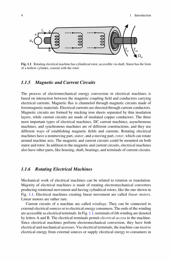
1.1.5 Magnetic and Current Circuits
The process of electromechanical energy conversion in electrical machines is
based on interaction between the magnetic coupling field and conductors carrying
electrical currents. Magnetic flux is channeled through magnetic circuits made of
ferromagnetic materials. Electrical currents are directed through current conductors.
Magnetic circuits are formed by stacking iron sheets separated by thin insulation
layers, while current circuits are made of insulated copper conductors. The three
most important types of electrical machines, DC current machines, asynchronous
machines, and synchronous machines are of different constructions, and they use
different ways of establishing magnetic fields and currents. Rotating electrical
machines have a nonmoving part, stator, and a moving part, rotor, which can rotatearound machine axis. The magnetic and current circuits could be mounted on both
stator and rotor. In addition to the magnetic and current circuits, electrical machines
also have other parts, like housing, shaft, bearings, and terminals of current circuits.
1.1.6 Rotating Electrical Machines
Mechanical work of electrical machines can be related to rotation or translation.
Majority of electrical machines is made of rotating electromechanical converters
producing rotational movement and having cylindrical rotors, like the one shown in
Fig. 1.1. Electrical machines creating linear movement are called linear motors.Linear motors are rather rare.
Current circuits of a machine are called windings. They can be connected to
external electrical sources or to electrical energy consumers. The ends of the winding
are accessible as electrical terminals. In Fig. 1.1, terminals of kth winding are denotedby letters A and B. The electrical terminals permit electrical access to the machine.
Since electrical machines perform electromechanical conversion, they have both
electrical and mechanical accesses. Via electrical terminals, the machine can receive
electrical energy from external sources or supply electrical energy to consumers in
Fig. 1.1 Rotating electrical machine has cylindrical rotor, accessible via shaft. Stator has the form
of a hollow cylinder, coaxial with the rotor
4 1 Introduction
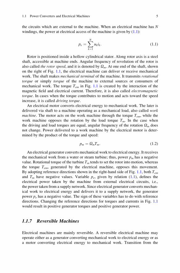
the circuits which are external to the machine. When an electrical machine has Nwindings, the power at electrical access of the machine is given by (1.1):
pe ¼XN
k¼1
ukik: (1.1)
Rotor is positioned inside a hollow cylindrical stator. Along rotor axis is a steel
shaft, accessible at machine ends. Angular frequency of revolution of the rotor is
also called the rotor speed, and it is denoted by Om. At one end of the shaft, shown
on the right of Fig. 1.1, the electrical machine can deliver or receive mechanical
work. The shaft makes mechanical terminal of the machine. It transmits rotationaltorque or simply torque of the machine to external sources or consumers of
mechanical work. The torque Tem in Fig. 1.1 is created by the interaction of the
magnetic field and electrical current. Therefore, it is also called electromagnetictorque. In cases when the torque contributes to motion and acts toward the speed
increase, it is called driving torque.An electrical motor converts electrical energy to mechanical work. The later is
delivered via shaft to a machine operating as a mechanical load, also called workmachine. The motor acts on the work machine through the torque Tem, while the
work machine opposes the rotation by the load torque Tm. In the case when
the driving and load torques are equal, angular frequency of the rotation Om does
not change. Power delivered to a work machine by the electrical motor is deter-
mined by the product of the torque and speed:
pm ¼ OmTm: (1.2)
An electrical generator converts mechanical work to electrical energy. It receives
the mechanical work from a water or steam turbine; thus, power pm has a negative
value. Rotational torque of the turbine Tm tends to set the rotor into motion, whereas
the torque Tem, generated by the electrical machine, opposes this movement.
By adopting reference directions shown in the right-hand side of Fig. 1.1, both Temand Tm have negative values. Variable pe, given by relation (1.1), defines the
electrical power taken by the machine from external electrical circuits, i.e.,
the power taken from a supply network. Since electrical generator converts mechan-
ical work to electrical energy and delivers it to a supply network, the generator
power pe has a negative value. The sign of these variables has to do with reference
directions. Changing the reference directions for torques and currents in Fig. 1.1
would result in positive generator torques and positive generator power.
1.1.7 Reversible Machines
Electrical machines are mainly reversible. A reversible electrical machine may
operate either as a generator converting mechanical work to electrical energy or as
a motor converting electrical energy to mechanical work. Transition from the
1.1 Power Converters and Electrical Machines 5
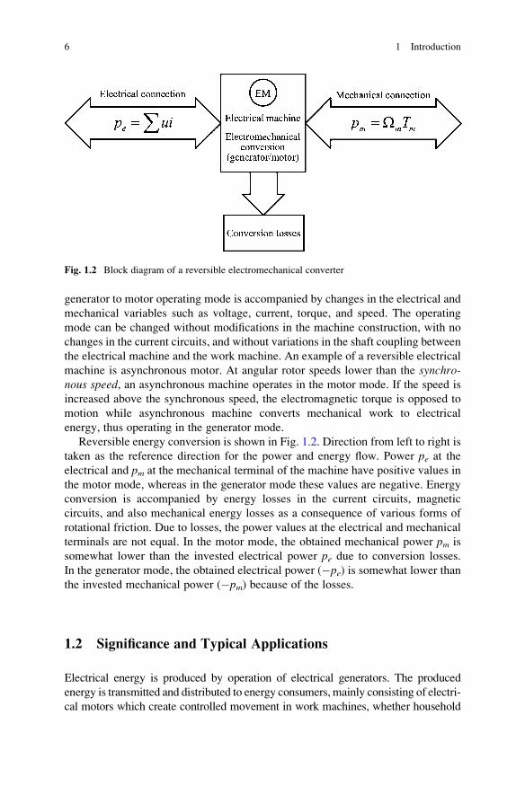
generator to motor operating mode is accompanied by changes in the electrical and
mechanical variables such as voltage, current, torque, and speed. The operating
mode can be changed without modifications in the machine construction, with no
changes in the current circuits, and without variations in the shaft coupling between
the electrical machine and the work machine. An example of a reversible electrical
machine is asynchronous motor. At angular rotor speeds lower than the synchro-nous speed, an asynchronous machine operates in the motor mode. If the speed is
increased above the synchronous speed, the electromagnetic torque is opposed to
motion while asynchronous machine converts mechanical work to electrical
energy, thus operating in the generator mode.
Reversible energy conversion is shown in Fig. 1.2. Direction from left to right is
taken as the reference direction for the power and energy flow. Power pe at theelectrical and pm at the mechanical terminal of the machine have positive values in
the motor mode, whereas in the generator mode these values are negative. Energy
conversion is accompanied by energy losses in the current circuits, magnetic
circuits, and also mechanical energy losses as a consequence of various forms of
rotational friction. Due to losses, the power values at the electrical and mechanical
terminals are not equal. In the motor mode, the obtained mechanical power pm is
somewhat lower than the invested electrical power pe due to conversion losses.
In the generator mode, the obtained electrical power (�pe) is somewhat lower than
the invested mechanical power (�pm) because of the losses.
1.2 Significance and Typical Applications
Electrical energy is produced by operation of electrical generators. The produced
energy is transmitted and distributed to energy consumers, mainly consisting of electri-
cal motors which create controlled movement in work machines, whether household
Fig. 1.2 Block diagram of a reversible electromechanical converter
6 1 Introduction
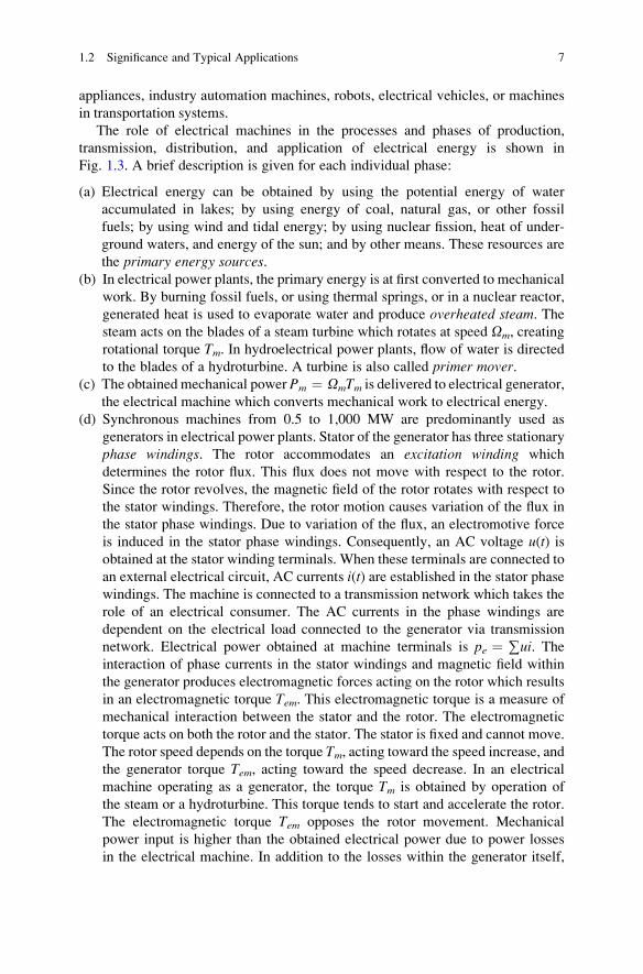
appliances, industry automation machines, robots, electrical vehicles, or machines
in transportation systems.
The role of electrical machines in the processes and phases of production,
transmission, distribution, and application of electrical energy is shown in
Fig. 1.3. A brief description is given for each individual phase:
(a) Electrical energy can be obtained by using the potential energy of water
accumulated in lakes; by using energy of coal, natural gas, or other fossil
fuels; by using wind and tidal energy; by using nuclear fission, heat of under-
ground waters, and energy of the sun; and by other means. These resources are
the primary energy sources.(b) In electrical power plants, the primary energy is at first converted to mechanical
work. By burning fossil fuels, or using thermal springs, or in a nuclear reactor,
generated heat is used to evaporate water and produce overheated steam. Thesteam acts on the blades of a steam turbine which rotates at speed Om, creating
rotational torque Tm. In hydroelectrical power plants, flow of water is directed
to the blades of a hydroturbine. A turbine is also called primer mover.(c) The obtained mechanical power Pm ¼ OmTm is delivered to electrical generator,
the electrical machine which converts mechanical work to electrical energy.
(d) Synchronous machines from 0.5 to 1,000 MW are predominantly used as
generators in electrical power plants. Stator of the generator has three stationary
phase windings. The rotor accommodates an excitation winding which
determines the rotor flux. This flux does not move with respect to the rotor.
Since the rotor revolves, the magnetic field of the rotor rotates with respect to
the stator windings. Therefore, the rotor motion causes variation of the flux in
the stator phase windings. Due to variation of the flux, an electromotive force
is induced in the stator phase windings. Consequently, an AC voltage u(t) isobtained at the stator winding terminals. When these terminals are connected to
an external electrical circuit, AC currents i(t) are established in the stator phasewindings. The machine is connected to a transmission network which takes the
role of an electrical consumer. The AC currents in the phase windings are
dependent on the electrical load connected to the generator via transmission
network. Electrical power obtained at machine terminals is pe ¼ ∑ui. Theinteraction of phase currents in the stator windings and magnetic field within
the generator produces electromagnetic forces acting on the rotor which results
in an electromagnetic torque Tem. This electromagnetic torque is a measure of
mechanical interaction between the stator and the rotor. The electromagnetic
torque acts on both the rotor and the stator. The stator is fixed and cannot move.
The rotor speed depends on the torque Tm, acting toward the speed increase, andthe generator torque Tem, acting toward the speed decrease. In an electrical
machine operating as a generator, the torque Tm is obtained by operation of
the steam or a hydroturbine. This torque tends to start and accelerate the rotor.
The electromagnetic torque Tem opposes the rotor movement. Mechanical
power input is higher than the obtained electrical power due to power losses
in the electrical machine. In addition to the losses within the generator itself,
1.2 Significance and Typical Applications 7
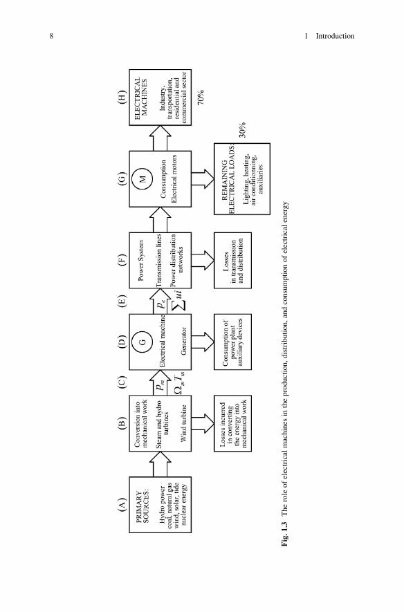
Fig.1.3
Therole
ofelectrical
machines
intheproduction,distribution,andconsumptionofelectrical
energy
8 1 Introduction
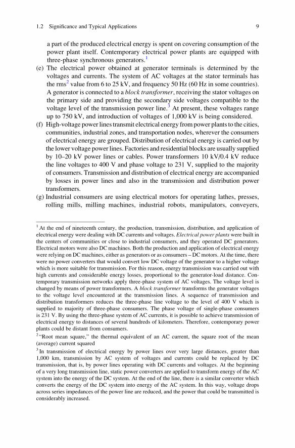
a part of the produced electrical energy is spent on covering consumption of the
power plant itself. Contemporary electrical power plants are equipped with
three-phase synchronous generators.1
(e) The electrical power obtained at generator terminals is determined by the
voltages and currents. The system of AC voltages at the stator terminals has
the rms2 value from 6 to 25 kV, and frequency 50 Hz (60 Hz in some countries).
A generator is connected to a block transformer, receiving the stator voltages onthe primary side and providing the secondary side voltages compatible to the
voltage level of the transmission power line.3 At present, these voltages range
up to 750 kV, and introduction of voltages of 1,000 kV is being considered.
(f) High-voltage power lines transmit electrical energy frompower plants to the cities,
communities, industrial zones, and transportation nodes, wherever the consumers
of electrical energy are grouped. Distribution of electrical energy is carried out by
the lower voltage power lines. Factories and residential blocks are usually supplied
by 10–20 kV power lines or cables. Power transformers 10 kV/0.4 kV reduce
the line voltages to 400 V and phase voltage to 231 V, supplied to the majority
of consumers. Transmission and distribution of electrical energy are accompanied
by losses in power lines and also in the transmission and distribution power
transformers.
(g) Industrial consumers are using electrical motors for operating lathes, presses,
rolling mills, milling machines, industrial robots, manipulators, conveyers,
1 At the end of nineteenth century, the production, transmission, distribution, and application of
electrical energy were dealing with DC currents and voltages. Electrical power plantswere built inthe centers of communities or close to industrial consumers, and they operated DC generators.
Electrical motors were also DC machines. Both the production and application of electrical energy
were relying on DCmachines, either as generators or as consumers – DCmotors. At the time, there
were no power converters that would convert low DC voltage of the generator to a higher voltage
which is more suitable for transmission. For this reason, energy transmission was carried out with
high currents and considerable energy losses, proportional to the generator-load distance. Con-
temporary transmission networks apply three-phase system of AC voltages. The voltage level is
changed by means of power transformers. A block transformer transforms the generator voltages
to the voltage level encountered at the transmission lines. A sequence of transmission and
distribution transformers reduces the three-phase line voltage to the level of 400 V which is
supplied to majority of three-phase consumers. The phase voltage of single-phase consumers
is 231 V. By using the three-phase system of AC currents, it is possible to achieve transmission of
electrical energy to distances of several hundreds of kilometers. Therefore, contemporary power
plants could be distant from consumers.2 “Root mean square,” the thermal equivalent of an AC current, the square root of the mean
(average) current squared3 In transmission of electrical energy by power lines over very large distances, greater than
1,000 km, transmission by AC system of voltages and currents could be replaced by DC
transmission, that is, by power lines operating with DC currents and voltages. At the beginning
of a very long transmission line, static power converters are applied to transform energy of the AC
system into the energy of the DC system. At the end of the line, there is a similar converter which
converts the energy of the DC system into energy of the AC system. In this way, voltage drops
across series impedances of the power line are reduced, and the power that could be transmitted is
considerably increased.
1.2 Significance and Typical Applications 9
mills, pumps for various fluids, ventilators, elevators, drills, forklifts, and other
equipment and devices involved in production systems and processes.
In electrical home appliances, motors are applied in air conditioners,
refrigerators, washing and dishwashing machines, freezers, mixers, mills,
blenders, record players, CD/DVD players, and computers and computer
peripherals. Approximately 8% of the total electrical energy consumption is
spent for supplying motors in transportation units like railway, city transport,
and electrical cars.
(h) In industrialized countries, 60–70% of the electrical energy production is
consumed by electrical machines providing mechanical power and controlling
motion in industry, traffic, offices, and homes. Therefore, it can be concluded
that most of the electrical energy produced by generators is consumed by
electrical motors which convert this energy to mechanical work. Electrical
motors are coupled mechanically to machines handling mechanical work and
power, carrying and transporting the goods, pumping fluids, or performing
other useful operations. Most electrical motors draw the electric power from
the three-phase distribution grid with line voltages of 400 V and line frequencyof 50(60) Hz. If the speed of electrical motor has to be varied, it is necessary to
use a static power converter between the motor terminals and the distribution
grid. The static power converters are power electronics devices comprising
semiconductor power switches. Their role is to convert the energy of line-
frequency voltages and currents and to provide the motor supply voltages and
currents with adjustable amplitude and frequency, suited to the motor needs.
1.3 Variables and Relations of Rotational Movement
Electrical machines are mainly rotating devices comprising a motionless stator
which accommodates a cylindrical rotor. The rotor revolves around the axis
which is common to both rotor and stator cylinders. Along this axis, the machine
has a steel shaft serving for transmission of the produced mechanical work to an
external work machine. There are also linear electrical machines wherein the
moving part performs translation and is subject to forces instead of torques. Their
use is restricted to solving particular problems in transportation and a relatively
small number of applications in robotics.
Position of rotor is denoted by ym, and this angle is expressed in radians. The firstderivative of the angle is mechanical speed of rotation, dym/dt ¼ Om, expressed in
radians per second. Sign of Om depends on the adopted reference direction. It is
adopted that positive direction of rotation is counterclockwise (CCW). Besides the
rotor mechanical speed, this book also studies rotation of the magnetic field and
rotation of other relevant electrical and magnetic quantities.
Speed of rotation of each of the considered variables will be denoted by the
upper case Greek letter O, whereas the lower case Greek letter o will be reserved
10 1 Introduction
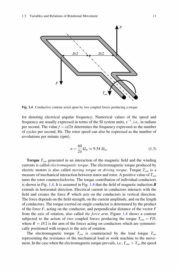
for denoting electrical angular frequency. Numerical values of the speed and
frequency are usually expressed in terms of the SI system units, s�1, i.e., in radians
per second. The value f ¼ o/2p determines the frequency expressed as the number
of cycles per second, Hz. The rotor speed can also be expressed as the number of
revolutions per minute (rpm),
n ¼ 60
2pOm � 9:54 Om: (1.3)
Torque Tem generated in an interaction of the magnetic field and the winding
currents is called electromagnetic torque. The electromagnetic torque produced by
electric motors is also called moving torque or driving torque. Torque Tem is a
measure of mechanical interaction between stator and rotor. A positive value of Temturns the rotor counterclockwise. The torque contribution of individual conductors
is shown in Fig. 1.4. It is assumed in Fig. 1.4 that the field of magnetic induction Bextends in horizontal direction. Electrical current in conductors interacts with the
field and creates the force F which acts on the conductors in vertical direction.
The force depends on the field strength, on the current amplitude, and on the length
of conductors. The torque exerted on single conductor is determined by the product
of the force F, acting on the conductor, and perpendicular distance of the vector Ffrom the axis of rotation, also called the force arm. Figure 1.4 shows a contour
subjected to the action of two coupled forces producing the torque Tem ¼ FD,where R ¼ D/2 is the arm of the forces acting on conductors which are symmetri-
cally positioned with respect to the axis of rotation.
The electromagnetic torque Tem is counteracted by the load torque Tm,representing the resistance of the mechanical load or work machine to the move-
ment. In the case when the electromagnetic torque prevails, i.e., Tem > Tm, the speed
Fig. 1.4 Conductive contour acted upon by two coupled forces producing a torque
1.3 Variables and Relations of Rotational Movement 11
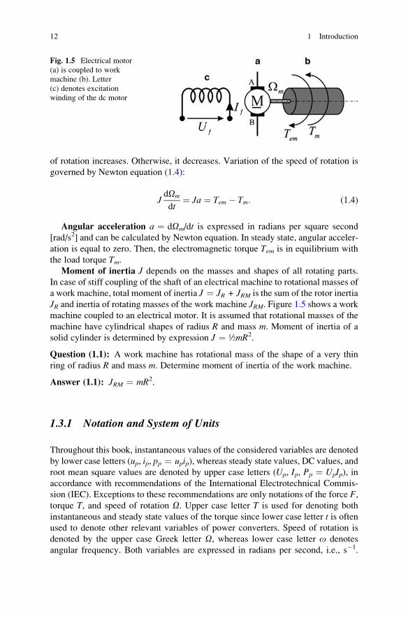
of rotation increases. Otherwise, it decreases. Variation of the speed of rotation is
governed by Newton equation (1.4):
JdOm
dt¼ Ja ¼ Tem � Tm: (1.4)
Angular acceleration a ¼ dOm/dt is expressed in radians per square second
[rad/s2] and can be calculated by Newton equation. In steady state, angular acceler-
ation is equal to zero. Then, the electromagnetic torque Tem is in equilibrium with
the load torque Tm.Moment of inertia J depends on the masses and shapes of all rotating parts.
In case of stiff coupling of the shaft of an electrical machine to rotational masses of
a work machine, total moment of inertia J ¼ JR + JRM is the sum of the rotor inertia
JR and inertia of rotating masses of the work machine JRM. Figure 1.5 shows a workmachine coupled to an electrical motor. It is assumed that rotational masses of the
machine have cylindrical shapes of radius R and mass m. Moment of inertia of a
solid cylinder is determined by expression J ¼ ½mR2.
Question (1.1): A work machine has rotational mass of the shape of a very thin
ring of radius R and mass m. Determine moment of inertia of the work machine.
Answer (1.1): JRM ¼ mR2.
1.3.1 Notation and System of Units
Throughout this book, instantaneous values of the considered variables are denoted
by lower case letters (up, ip, pp ¼ upip), whereas steady state values, DC values, and
root mean square values are denoted by upper case letters (Up, Ip, Pp ¼ UpIp), inaccordance with recommendations of the International Electrotechnical Commis-
sion (IEC). Exceptions to these recommendations are only notations of the force F,torque T, and speed of rotation O. Upper case letter T is used for denoting both
instantaneous and steady state values of the torque since lower case letter t is oftenused to denote other relevant variables of power converters. Speed of rotation is
denoted by the upper case Greek letter O, whereas lower case letter o denotes
angular frequency. Both variables are expressed in radians per second, i.e., s�1.
Fig. 1.5 Electrical motor
(a) is coupled to work
machine (b). Letter
(c) denotes excitation
winding of the dc motor
12 1 Introduction
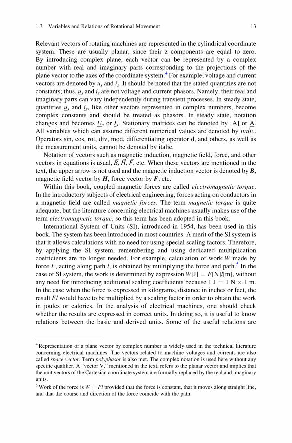
Relevant vectors of rotating machines are represented in the cylindrical coordinate
system. These are usually planar, since their z components are equal to zero.
By introducing complex plane, each vector can be represented by a complex
number with real and imaginary parts corresponding to the projections of the
plane vector to the axes of the coordinate system.4 For example, voltage and current
vectors are denoted by us and is. It should be noted that the stated quantities are notconstants; thus, us and is are not voltage and current phasors. Namely, their real and
imaginary parts can vary independently during transient processes. In steady state,
quantities us and is, like other vectors represented in complex numbers, become
complex constants and should be treated as phasors. In steady state, notation
changes and becomes Us or Is. Stationary matrices can be denoted by [A] or A.
All variables which can assume different numerical values are denoted by italic.Operators sin, cos, rot, div, mod, differentiating operator d, and others, as well as
the measurement units, cannot be denoted by italic.
Notation of vectors such as magnetic induction, magnetic field, force, and other
vectors in equations is usual, ~B, ~H, ~F, etc. When these vectors are mentioned in the
text, the upper arrow is not used and the magnetic induction vector is denoted by B,magnetic field vector by H, force vector by F, etc.
Within this book, coupled magnetic forces are called electromagnetic torque.In the introductory subjects of electrical engineering, forces acting on conductors in
a magnetic field are called magnetic forces. The term magnetic torque is quite
adequate, but the literature concerning electrical machines usually makes use of the
term electromagnetic torque, so this term has been adopted in this book.
International System of Units (SI), introduced in 1954, has been used in this
book. The system has been introduced in most countries. A merit of the SI system is
that it allows calculations with no need for using special scaling factors. Therefore,
by applying the SI system, remembering and using dedicated multiplication
coefficients are no longer needed. For example, calculation of work W made by
force F, acting along path l, is obtained by multiplying the force and path.5 In the
case of SI system, the work is determined by expressionW[J] ¼ F[N]l[m], without
any need for introducing additional scaling coefficients because 1 J ¼ 1 N � 1 m.
In the case when the force is expressed in kilograms, distance in inches or feet, the
result Fl would have to be multiplied by a scaling factor in order to obtain the work
in joules or calories. In the analysis of electrical machines, one should check
whether the results are expressed in correct units. In doing so, it is useful to know
relations between the basic and derived units. Some of the useful relations are
4 Representation of a plane vector by complex number is widely used in the technical literature
concerning electrical machines. The vectors related to machine voltages and currents are also
called space vector. Term polyphasor is also met. The complex notation is used here without any
specific qualifier. A “vector V,” mentioned in the text, refers to the planar vector and implies that
the unit vectors of the Cartesian coordinate system are formally replaced by the real and imaginary
units.5Work of the force isW ¼ Fl provided that the force is constant, that it moves along straight line,
and that the course and direction of the force coincide with the path.
1.3 Variables and Relations of Rotational Movement 13
[Vs] ¼ [Wb], [Nm rad/s] ¼ [W], [Nm rad] ¼ [J], [AO] ¼ [V], [AH] ¼ [Wb] ¼[Vs], etc.
Within this book, the rated values are denoted a subscript n, such as in Un or In.
1.4 Target Knowledge and Skills
Knowledge of electrical machines is a basis for successful activity of an electrical
engineer. A large number of applications and systems, designed or used by an
electrical engineer, contain one or more electrical machines. Characteristics of these
applications and systems are usually determined by the performances of electrical
machines, their dimensions, mass, efficiency, peak torque capability, and speed range,
as well as control characteristics and dynamic response. For this reason, it is necessary
to acquire the knowledge and skills to understand basic operation principles of
electrical machines. Basic understanding of mechanical and electrical characteristics
of electrical machines is required to specify and design their power supply and
controls. The knowledge concerning the origin and nature of energy losses in electrical
machines is required to specify and design their cooling and conceive their loss-
minimized use.
The most significant challenges in developing novel solutions are design of the
magnetic circuit and windings, resolving power supply problems, and devising
control laws. Machines should be designed to have the smallest possible dimen-
sions and mass, and to operate with low energy losses. At the same time, machines
should be as cheap and robust as possible. At present, the power supply and controls
of electrical machines are carried out by using static power converters and digital
signal controllers. Some of the goals of generator control are reduction of losses,
reduction of electromagnetic and mechanical stress of materials, as well as increas-
ing the power-to-mass ratio, also called specific power. Motor control aims at
achieving as high as possible accuracy and speed of reaching the torque and
speed targets required for performing desired movement of a work machine.
This book contains the basic knowledge concerning electrical machines neces-
sary for future electrical engineers. The approach starts from the basic role and
function of the machine. The characteristics of machine electrical and mechanical
accesses (ports) are analyzed in order to define the mathematical model, equivalent
circuits, and mechanical characteristics. This book deals with the elements of
machine design, problems of heating and cooling, and also with specific imper-
fections of magnetic circuits and windings. The depth of the study is suited for
understanding the operating principles of main machine types, for acquiring basic
knowledge on power supply topologies, and for comprehending essential concepts
of machine controls. Rotational electromechanical converters are studied in this
book, whereas the power transformers are omitted.
14 1 Introduction
1.4.1 Basic Characteristics of Electrical Machines
Design, specification, and analysis of electrical machine applications require an
adequate idea on the size, mass, construction, reliability, and losses. The basic
knowledge of electrical machines is required for designing systems incorporating
electrical machines and solving the problems of power supply and controls. Basic
electrical machine concepts are also required for designing monitoring and protec-
tion systems, designing servomotor controllers in robotics, and designing controls
and protections for synchronous generators in electrical power plants. The knowl-
edge of electrical machines is required in all situations and tasks likely to be put
before an electrical engineer in industry, power generation, industrial automation,
and robotics.
1.4.2 Equivalent Circuits
The torque and speed control of an electrical machine is performed by establishing
the winding voltages and currents by means of an appropriate power supply. Design
or selection of power supply for a given electrical machine requires establishing
relations between the machine flux, torque, voltages, and currents. The steady
state relations are described by a steady state equivalent circuit. The equivalent
circuit is an electrical circuit containing resistors, inductances, and electromotive
forces. At steady state, with constant speed and with the given amplitude and
frequency of the supply, the equivalent circuit allows calculation of currents in
the windings. Based upon the currents determined from the equivalent circuit, it is
possible to calculate the steady state flux, torque, power of electromechanical
conversion, and power losses.
1.4.3 Mechanical Characteristic
For the given voltage and frequency of the power supply, the calculation of the
steady state values of the machine speed and torque requires the torque-speed
characteristic of the work machine which is attached to the shaft and acts as
mechanical load. The relation Tm�Om of the work machine is also calledmechani-cal characteristic of the load, and it is expressed by the function Tm(Om). In a like
manner, mechanical characteristic of the electrical machine is the relation between
the electromagnetic torque Tem and the rotor speed Om in the steady state. It is
possible to express the mechanical characteristic by function Tem(Om) and present it
graphically in the Tem-Om plane. Determination of the mechanical characteristic can
be carried out by using mathematical model of the machine. The steady state
operating point is found at the intersection of the two mechanical characteristics,
Tem(Om) and Tm(Om).
1.4 Target Knowledge and Skills 15
1.4.4 Transient Processes in Electrical Machines
The equivalent circuit and mechanical characteristics can be used for the steady
state analysis of electrical machines, i.e., in the operating modes where the torque,
flux, speed of rotation, currents, and voltages do not change their values,
amplitudes, or frequencies. There are numerous applications where it is required
to accomplish fast variations of the torque and speed of rotation. In these
applications, it is necessary to have a mathematical representation of the machine
which reflects its behavior during transients. This representation is called mathe-matical model. Deriving the mathematical model, one cannot start from the
assumption that machine operates in steady state. For this reason, such model is
also called dynamic model. Examples of electrical machine applications where the
dynamic model has to be used are the controls of industrial manipulators and robots
and propulsion of electrical vehicles. The motion control implies variations of
speed and position along a predefined trajectory of a tool, work piece, vehicle, or
an arm of an industrial robot. Whenever the controlled object falls out of the desired
trajectory, it is necessary to assert a relatively fast change of the force (or torque) in
order to drive the controlled object back to the desired path and annihilate the error.
The task of the position (or speed) controller is to calculate the force (torque) to be
applied in order to remove the detected position (or speed) discrepancy. The task of
electrical motor is to deliver desired torque as fast and accurate as possible. In such
servo applications, electrical motors are required to realize very fast changes of
torque in order to remove the influence of variable motion resistances on the speed
and position of the controlled objects. The analysis of operation of an electrical
machine used as a servomotor in motion control applications requires thorough
knowledge of transient processes within the machine.
Another case where the mathematical model is required is the analysis of
transient processes in grid-connected synchronous generators operating in electrical
power plants. Sudden rises and falls of electrical consumption in transmission
networks are caused by switching on and off of large consumers, or quite frequently
by short circuits. They affect generators as an abrupt change of their electrical load.
The analysis of generator voltages and currents during transients cannot be
performed by using the steady state equivalent circuit. Instead, it is required to
have a mathematical model depicting the transient phenomena within the machine.
1.4.5 Mathematical Model
The mathematical model is represented by a set of algebraic and differential
equations describing behavior of a machine during transients and in steady states.
The voltage balance equations express the equilibrium of voltage in the machine
windings, and they have the form u ¼ Ri + dC/dt. The change of the rotor speed isdetermined by Newton differential equation J dOm/dt ¼ Tem � Tm. Quantities such
16 1 Introduction
as J and R are parameters, while Om and C are variables describing the state of the
machine (state variables). An electrical engineer needs the model of electrical
machine for performing the analysis of the energy conversion processes, for the
analysis of conversion losses, for designing of the machine power supply and
controls, as well as for solving the problems that may occur during machine
applications. For this reason, it is necessary to have a relatively simple and intuitive
model so that it can present the processes and states of the machine in a concise and
clear way. A good model should be thorough and concise outline of the relevant
phenomena within the machine, suitable for making conclusions and taking
decisions as regards power supply, controls, and use of the electrical machines.
There are aspects and phenomena within the machine which are not relevant for
problems under the scope because they influence operation of an electrical machine
to a very limited extent. They are called secondary or parasitic effects, as they are
usually neglected in order to obtain a simpler, more practical mathematical model.
As an example, the energy density we ¼ e E2/2 of electric field E within electrical
machines can be neglected. It is lower than the energy density of magnetic field
by several orders of magnitude. In the process of modeling, other justifiable
omissions are adopted in order to obtain a simplified model which still matches
the purpose. For the problem under consideration, the most appropriate model is
the simplest one, yet depicting all the relevant dynamic phenomena. Justifiable
omissions of secondary effects lead to mathematical models that are less complex
and more intuitive. With such models, it is easier to overview the main features of
the system. The problem solving and decision-making process becomes quicker
and straightforward.
In electrical engineering, the model is usually a set of differential equations
describing behavior of a system. Model of an electrical machine, or a transformer,
can be reduced to the equivalent circuit describing its steady state operation. On the
basis of the model, it is possible to determine the mechanical characteristic of
the machine.
1.5 Adopted Approach and Analysis Steps
In general, the material presented in this book is intended for electrical engineering
students. The basic knowledge of mathematics, physics, and electricity is practi-
cally applied in studying electrical machines, by many students met for the very
first time. The approach starts with general notion and then goes to detail. It allows
the beginners to perceive at first the basic purpose, appearance, and fundamental
characteristics of electrical machines. Following the introductory chapters, this
book investigates operating modes in typical applications and studies equivalent
circuits, mechanical characteristics, power supply topologies and controls, as well
as the losses and the problems in exploitation. Later on, the focus is turned to details
related to the three main types of electrical machines.
1.5 Adopted Approach and Analysis Steps 17
The attention is directed toward DC, asynchronous, and synchronous machines.
In this book, other types of electrical machines have not been studied in detail.
The problems associated with design of electrical machines are briefly mentioned.
The winding techniques, magnetic circuit design, analysis of secondary phenom-
ena, the secondary and parasitic losses, and construction details have been left out
for further studies. The main purpose of this book is introducing the reader to
the role of electrical machines and studying their electrical and mechanical
properties in order to acquire the ability to specify their electrical and mechanical
characteristics, to define their power supplies and control laws, and to design
systems with electrical motors and generators.
The study of electrical machines starts by an introduction to the basic principles
of operation and with a survey of functions of electrical generators and motors in
their most frequent applications. The analysis steps include the principles of
electromechanical conversion and study the conversion process by taking the
example of an electrostatic machine. Energy of the coupling electrical field is
analyzed along with the process of energy exchange between the field, the electrical
source, and the mechanical port. The study proceeds with the analysis of a simple
electromechanical converter with magnetic coupling field. Construction of the
magnetic circuit and windings of the machine are followed by specification of
conversion losses. Subsequently, rotational electromechanical converters with
magnetic coupling are considered, along with the rotating electrical machines
which are the main subject of this study. The basic notions and definitions include
the magnetic resistances and circuits, concentrated and distributed windings,
methods of calculating the flux per turn and the winding flux, and the expressions
for the winding self-inductances, mutual inductances, and leakage inductances.
Magnetomotive forces of the winding are explained and analyzed, as well as
electromotive forces induced in concentrated and distributed windings. The mag-
netic field in the air gap is analyzed and applied in modeling the electromechanical
conversion in cylindrical machines. The electromagnetic torque and the power of
electromechanical conversion are expressed in terms of flux vectors and magne-
tomotive forces. The concept and creation of rotating magnetic field are detailed
and used to describe the difference between direct current (DC) machines and
alternating current (AC) machines. The mathematical model of a cylindrical
machine with the windings having N coils is derived, along with the expressions
for electrical power, mechanical power, and power losses in the windings, magnetic
circuit, and the mechanical subsystem. The secondary phenomena that are usually
neglected in the analysis of electrical machines are specified and explained. At the
same time, some sample applications and operating conditions are named where
the secondary phenomena cannot be excluded from the analysis.
The introduction is followed by the chapters dealing with DC machines, asyn-
chronousmachines (AM), and synchronousmachines (SM). Each chapter starts with
basic description and the operating principles of the relevant machine, followed by
the most significant aspects of its construction, description of its merits, the most
frequent applications, and meaningful shortcomings. The expressions are derived
18 1 Introduction
for the magnetomotive force, flux, electromotive force, torque, and conversion
power. Mathematical model is derived for the machine under consideration, describ-
ing its behavior during transient processes and providing the grounds for obtaining
the equivalent circuits and mechanical characteristics. In the case of AC electrical
machines, the modeling includes introduction of the three-phase/two-phase coordi-
nate transformation (Clarke transform) and coordinate transformation from the
stationary coordinate frame to the revolving coordinate frame (dq or Park
transform).
The equivalent electrical circuits of the machine are derived from the steady
state analysis. They are used to calculate the currents, voltages, flux, torque, and
power at steady states, where the supply voltage, the load torque Tm, and the speed
of rotation are known and unchanging. The mathematical model is also used to
obtain the mechanical characteristic which gives the steady state relation of the
machine speed and torque delivered to the shaft. For each electrical machine,
the operating regimes sustainable in the steady state are analyzed and formulated
as the steady state operating area in the Tem-Om plane. Likewise, the transientoperating area of the Tem-Om plane is defined, representing the transient operating
regimes attainable in short time intervals.
Particular attention is paid to conversion losses. The losses in the windings and
magnetic circuits are analyzed in depth, along with heating of electrical machines
and the methods of their cooling. The highest sustainable values of the current,
power, and torque are defined and explored. These values and the highest sustain-
able values of other relevant quantities are called the rated values.6 The need for
operation in the region of field weakening is emphasized, and the relevant relations
and characteristics are derived.
The transient operating area is analyzed for DC and AC machines. It is derived
from the short-term overload capabilities of mechanical and electrical ports of
electrical machines. The analysis takes into account the impact of peak current
and peak voltage capabilities of the electrical power supply on the machine
transient performance. Basic information concerning the supply, controls, and
typical power converter topologies used in conjunction with the electrical machine
is given for DC, asynchronous, and synchronous machines.
6 The rated values are the highest permissible values of the machine currents, voltages, power,
speed, and torque in a continuous service. Permanent operation with higher values will damage the
machine’s vital parts due to phenomena such as overheating. They are usually the result of
engineering calculation, and they also represent an important property of the machine. The rated
values are usually related to specified ambient temperature. Typically, the rated power is the
maximum power the electrical machine can deliver continuously at 40�C ambient temperature.
The values written on the machine plate or in manufacturer’s specifications are called nameplate ornominal values. The nominal and rated values are usually equal. In rare cases, manufacturer may
have the reason to declare the nominal values lower than the rated values. Within this book, it is
assumed that the nominal values correspond to the rated. They are denoted by a lowercase
subscript n, such as in Un or In.
1.5 Adopted Approach and Analysis Steps 19
1.5.1 Prerequisites
Precondition to understanding analysis and considerations in this book, accepting
the knowledge, acquiring the target skills, and solving the problems is the knowl-
edge of mathematics, physics, and basic electrical engineering which is normally
taught at the first year of undergraduate studies of engineering. It is required to know
the basic laws of motion and practical relations concerning rotation and translation.
Required background includes the steady state electrical and magnetic fields, the
basic characteristics of dielectric and ferromagnetic materials, and elementary
boundary conditions for electrostatic and magnetic fields. Chapter 2, Electromag-netic Energy Conversion, deals with the analysis of the energy and forces associatedwith electrostatic and magnetic fields in dielectrics, ferromagnetics, and air. Further
on, analysis includes solving simple electric circuits with DC or AC currents.
In addition, the analysis extends on the magnetic circuits involving magnetomotive
forces (magnetic voltages), flux linkage, andmagnetic resistances. The basic laws of
electrical engineering should be known, like Faraday law on electromagnetic induc-
tion, Ampere law, Lorentz law, and Kirchhoff laws and similar. The study includes
spatial distribution of the current, field, and energy. Therefore, coordinates in
the Cartesian or in the cylindrical coordinate systems will be used along with the
corresponding unit vectors. A consistent effort is sustained throughout this book to
make the developments material accessible to readers not familiar with spatial
derivatives, such as rotor (curl, rot) or divergence (div). Therefore, familiarity
with Maxwell differential equations is not inevitable. Instead of differential form
of Maxwell laws, it is sufficient to know their integral form, such as Ampere law.
The skill in handling complex numbers and phasors is required, as well as dealing
with scalar and vector products of vectors. For determining direction of a vector
product, one should be familiar with the right-hand rule. Also required are the
abilities of representing and perceiving relations between three-dimensional objects,
of identifying closed surfaces defining a domain, and of contours defining a surface
and surface normals. Within this book, the problem solving involves relatively
simple line and surface integrals and solution of first-order linear differential
equations. An experience in reducing differential equations to algebraic equations
by applying Laplace transform and the ability of performing basic operations with
matrices and vectors are also useful.
1.6 Notes on Converter Fed Variable Speed Machines
This book has not been written with an intention to prepare a reader for designing
electrical machines. The main goal is studying the electrical and mechanical
characteristics of electrical machines from the user’s point of view, with an intention
to prepare a reader for selecting an adequate machine, for solving the problems
associated with the power supply and controls, and for handling the problems that
may appear during operation of electrical motors and generators. The specific
20 1 Introduction
knowledge required for designing electrical machines is left out for further studies.
The prerequisite for exploring further is a thorough acceptance of the knowledge and
skills comprised within this book. The need for skilled designers of electrical
machines is higher than before. Some of the reasons for this are the following:
• During the last century, electrical machines were designed to operate from the
grid, with constant voltages and with the line frequency. Development of static
power converters, providing three-phase voltages of variable frequency and
amplitude, permits the power supply of an electrical motor to be adjusted to
the speed and torque. Most new designs with electrical motors include static
power converters that convert the energy received from the grid into the form
best suited to the actual speed and torque. The voltage and frequency can be
adjusted to reduce the power losses while delivering the reference torque at
given speed. Therefore, there is an emerging quest for electrical machines
designed to operate in conjunction with static power converters and variable
frequency power supply.
• Applications of electrical motors for propelling electrical vehicles or driving
industrial robots often require the rotor speed exceeding several hundreds of
revolutions per second, which requires the power supply frequencies of the order
of f > 500 Hz. Therefore, within contemporary servomotors and traction
motors, electrical currents and magnetic induction pulsate at the same frequency.
Fast variation of magnetic field requires application of new magnetic materials
and novel design solutions for magnetic circuits. The increased frequencies of
electric currents demand new solutions for making the windings.
• Propelling industrial robots requires electrical motors having a fast response and
low inertia. Therefore, it is required to design synchronous motors having
permanent magnets in their rotors, with the rotor shape and size resulting in a
low inertia and fast acceleration, such as a disc or a hollow cylinder with double
air gap.
• An increased interest in alternative and renewable power sources requires design
of novel synchronous generators, suitable for the operation in conjunction with
wind turbines, tidal turbines, and similar. The speed and the operating frequency
are variable, while in some cases, generators operate at a very low speed. At the
same time, the inertia and weight of generators should be low, with the lowest
possible power losses.
• Construction of thermal electric power plants with supercritical steam pressure
enables design of a single block in excess of 1 GW. Mechanical power of the
block, obtained from a steam turbine, is converted to electrical energy by means
of a synchronous generator operating at the line frequency of 50 Hz. Designing
generators of this high power demands application of new design solutions, new
insulating and ferromagnetic materials, and new cooling methods and systems.
The need to increase the production of electrical energy and the need to reduce
the heat released to the environment can be alleviated by reducing the losses and
increasing the energy efficiency � of electrical machines. The efficiency of
generators and motors can be increased by adequate control, but also by designing
novel electrical machines and applying new materials in their construction.
1.6 Notes on Converter Fed Variable Speed Machines 21
1.7 Remarks on High Efficiency Machines
Reduction in power losses increases the energy efficiency of electrical machines
and relieves the problem of their cooling. As all the machine losses eventually turn
into heat, the loss reduction diminishes the heat emitted to the environment. The
heat released by electrical machines is a form of environmental pollution, and it
should be kept low. Considering the fact that industrial countries use more than 2/3
of their electrical energy in electrical motors, the loss reduction in electrical
machines has the greatest potential of energy saving. In addition, an efficient heat
removal (cooling) often requires specific engineering solutions, increasing in this
way the cost and complexity of the design. For these reasons, there is an increasing
need for designing new, more efficient electrical machines and to devise their
controls that would reduce the losses. Designing new solutions for electrical
generators and motors requires a thorough basic knowledge on their operating
principles, and it is bound to use novel ferromagnetic materials and new design
concepts. One example is the use of permanent magnet excitation which eliminates
the excitation winding and cuts down the rotor losses of synchronous machines.
Besides, an efficient electromechanical conversion requires as well new solutions
for the machine supply. Most of contemporary machines do not have a direct
connection to the grid and do not operate with line-frequency voltages and currents.
Instead, they are fed from static power converters which transform the grid supply
to the form which is consistent with an efficient operation of the machine. Supply
from a static power converter allows for the flux changes and selection of the flux
level which results in the lowest power losses. Successful design of electrical
machines supplied from static power converters requires a thorough knowledge
on electrical and magnetic fields within the machine, as well as the knowledge on
the energy conversion processes taking place within switching power converters.
1.8 Remarks on Iron and Copper Usage
On a wider scale, the energy efficiency of electrical machines includes as well the
amount of energy consumed in the course of themachine production.Manufacturing
of electrolytic copper and aluminum and making of laminated steel sheets require
large amounts of energy. For this reason, the machine that uses fewer raw materials
is likely to be the more efficient one. Construction of electrical machines has certain
similarities with the construction of power transformers. In both cases, the appliance
has a magnetic circuit and some electrical current circuits. Traditionally, magnetic
circuits are made of laminated steel sheets, whereas electric circuits (windings) are
made of insulated copper conductors. Both transformers and electrical machines are
used within systems comprising energy converters, semiconductor switches,
sensors, microprocessor control systems, and the associated software. The decisive
factor which governs the price of the whole system is the iron and copper weight
22 1 Introduction
involved. Namely, production of semiconductor devices requires relatively small
quantities of raw materials, such as the silicon ingot, some donor and acceptor
impurities, and relatively small quantities of ceramic or plastic materials for the
casing. Moreover, development, design, and software production costs have an
insignificant contribution to the cost in series production. Therefore, it is significant
to design and manufacture units and systems with reduced consumption of iron and
copper. Reducing the quantities of rawmaterials can be accomplished in three ways:
In the system design phase, the operating conditions of electrical machines
involved in the system can be planned so as to manufacture them with a reduced
consumption of iron and copper.
In the electrical machine design phase, it is possible to make the magnetic and
electric circuits in a manner that saves on raw materials. As an example, four-pole7
machines make a better use of the magnetic circuit than two-pole machines.
During the operation of electrical machine supplied from a static power
converter, it is possible to use the control methods that maximize the torque and
power available from the given magnetic and electric circuits. In this way, there is
an increase in the specific torque and specific power.8 Given the torque and power
requirements, it is possible to design and make the electrical machine with less iron
and less copper.
Contemporary computer tools for design of electrical machines allow antici-
pation of their characteristics prior to making and testing a prototype. This
facilitates and speeds up the design process. Moreover, it becomes possible to test
several different solutions and approaches over a relatively short period of time.
Most of the software packages make use of the finite element analysis (FEM) of
electrical, magnetic, mechanical, and thermal processes. Designing with computer
tools brings up the risk of inadvertent errors. The problems arise in cases when
designer pretends that the tool performs the creative part of the job. A computer tool
will give an output for each set of input data, whether the input makes sense or not.
Therefore, a user has to possess certain experience in design, in order to interpret
properly the obtained results and notice errors and contradictions. A conservative
use of computer tools consists of using computer for quick completion of automatic
tasks and calculations which the designer would have performed himself if he had
sufficient time.
7 The operation of electrical machines involving multiple pairs of magnetic poles will be explained
in chapter on asynchronous machines.8 For the given electrical machine, specific torque is the ratio between the available torque and the
mass (or volume) of the machine. Hence, it is the torque per unit mass (or volume). The same holds
for the specific power. With higher specific torque (or power), electrical machine is smaller and/or
lighter for the same task.
1.8 Remarks on Iron and Copper Usage 23
Chapter 2
Electromechanical Energy Conversion
Electrical machines contain stationary and moving parts coupled by an electrical or
magnetic field. The field acts on the machine parts and plays key role in the process
of electromechanical conversion. For this reason, it is often referred to as the
coupling field. This chapter presents the most significant principles of creating a
force or torque on the machine moving parts. In all the cases considered, the force
appears due to the action of the electrostatic or magnetic field on the moving parts
of the machine. Depending on the nature of the coupling field, the machines can be
magnetic or electrostatic.
2.1 Lorentz Force
Electrical machines perform conversion of electrical energy to mechanical work or
conversion of mechanical work to electrical energy. The basic principles involved
in the process of electromechanical conversion are presented in the considerations
which follow.
One of the laws of physics which is basic for electromechanical conversion is
Lorentz law which determines the force acting upon a charge Q moving with a
speed v in the electrical and magnetic fields:
~F ¼ Q~Eþ Q ~v� ~B� �
: (2.1)
In electrical machines, the operation is most often based on the magnetic
coupling field. Conductors and ferromagnetic parts in a magnetic field are subjected
to the action of electromagnetic forces. Magnetic induction B in (2.1) is also called
flux density. Electrical current existing in the conductor is a directed motion of
electrical charges. Therefore, (2.1) can be used to determine the force acting upon
conductors carrying electrical currents.
S.N. Vukosavic, Electrical Machines, Power Electronics and Power Systems,
DOI 10.1007/978-1-4614-0400-2_2, # Springer Science+Business Media New York 2013
25
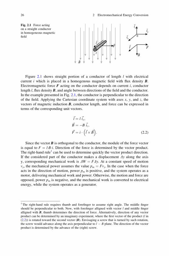
Figure 2.1 shows straight portion of a conductor of length l with electrical
current i which is placed in a homogenous magnetic field with flux density B.Electromagnetic force F acting on the conductor depends on current i, conductorlength l, flux density B, and angle between directions of the field and the conductor.In the example presented in Fig. 2.1, the conductor is perpendicular to the direction
of the field. Applying the Cartesian coordinate system with axes x, y, and z, thevectors of magnetic induction B, conductor length, and force can be expressed in
terms of the corresponding unit vectors.
~l ¼ l~ix;
~B ¼ �B~iz;
~F ¼ i � ~l� ~B� �
: (2.2)
Since the vector B is orthogonal to the conductor, the module of the force vector
is equal to F ¼ l�B�i. Direction of the force is determined by the vector product.
The right-hand rule1 can be used to determine quickly the vector product direction.
If the considered part of the conductor makes a displacement Dy along the axis
y, corresponding mechanical work is DW ¼ FDy. At a constant speed of motion
vy, the mechanical power assumes the value pm ¼ Fvy. In the case when the force
acts in the direction of motion, power pm is positive, and the system operates as a
motor, delivering mechanical work and power. Otherwise, the motion and force are
opposed, power pm is negative, and the mechanical work is converted to electrical
energy, while the system operates as a generator.
1 The right-hand rule requires thumb and forefinger to assume right angle. The middle finger
should be perpendicular to both. Now, with forefinger alligned with vector l and middle finger
alligned with B, thumb determines the direction of force. Alternatively, direction of any vector
product can be determined by an imaginary experiment, where the first vector of the product (l in(2.2)) is rotated toward the second vector (B). Envisaging a screw that is turned by such rotation,
the screw would advance along the axis perpendicular to l � B plane. The direction of the vector
product is determined by the advance of the (right) screw.
Fig. 2.1 Force acting
on a straight conductor
in homogeneous magnetic
field
26 2 Electromechanical Energy Conversion
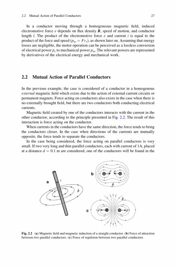
In a conductor moving through a homogeneous magnetic field, induced
electromotive force e depends on flux density B, speed of motion, and conductor
length l. The product of the electromotive force e and current i is equal to the
product of the force and speed (pm ¼ Fvy), as shown later on. Assuming that energy
losses are negligible, the motor operation can be perceived as a lossless conversion
of electrical power pe to mechanical power pm. The relevant powers are representedby derivatives of the electrical energy and mechanical work.
2.2 Mutual Action of Parallel Conductors
In the previous example, the case is considered of a conductor in a homogenous
external magnetic field which exists due to the action of external current circuits or
permanent magnets. Force acting on conductors also exists in the case when there is
no externally brought field, but there are two conductors both conducting electrical
currents.
Magnetic field created by one of the conductors interacts with the current in the
other conductor, according to the principle presented in Fig. 2.2. The result of this
interaction is force acting on the conductor.
When currents in the conductors have the same direction, the force tends to bring
the conductors closer. In the case when directions of the currents are mutually
opposite, the force tends to separate the conductors.
In the case being considered, the force acting on parallel conductors is very
small. If two very long and thin parallel conductors, each with current of 1A, placed
at a distance d ¼ 0.1 m are considered, one of the conductors will be found in the
Fig. 2.2 (a) Magnetic field and magnetic induction of a straight conductor. (b) Force of attraction
between two parallel conductors. (c) Force of repulsion between two parallel conductors
2.2 Mutual Action of Parallel Conductors 27
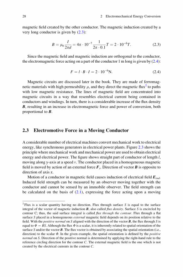
magnetic field created by the other conductor. The magnetic induction created by a
very long conductor is given by (2.3):
B ¼ m0I
2pd¼ 4p � 10�7 1
2p � 0:1 T ¼ 2 � 10�6T: (2.3)
Since the magnetic field and magnetic induction are orthogonal to the conductor,
the electromagnetic force acting on a part of the conductor 1m long is given by (2.4):
F ¼ l � B � I ¼ 2 � 10�6N: (2.4)
Magnetic circuits are discussed later in the book. They are made of ferromag-
netic materials with high permeability m, and they direct the magnetic flux2 to paths
with low magnetic resistance. The lines of magnetic field are concentrated into
magnetic circuits in a way that resembles electrical current being contained in
conductors and windings. In turn, there is a considerable increase of the flux density
B, resulting in an increase in electromagnetic force and power of conversion, both
proportional to B.
2.3 Electromotive Force in a Moving Conductor
A considerable number of electrical machines convert mechanical work to electrical
energy, like synchronous generators in electrical power plants. Figure 2.3 shows the
principle where mechanical work andmechanical power are used to obtain electrical
energy and electrical power. The figure shows straight part of conductor of length l,moving along y-axis at a speed v. The conductor placed in a homogeneous magnetic
field is moved by action of an external force Fs. Direction of vector B is opposite to
direction of axis z.
Motion of a conductor in magnetic field causes induction of electrical field Eind.Induced field strength can be measured by an observer moving together with the
conductor and cannot be sensed by an immobile observer. The field strength can
be calculated on the basis of (2.1), expressing the force acting upon a moving
2 Flux is a scalar quantity having no direction. Flux through surface S is equal to the surface
integral of the vector of magnetic induction B, also called flux density. Surface S is encircled by
contour C; thus, the said surface integral is called flux through the contour. Flux through a flat
surface S placed in a homogeneous external magnetic field depends on its position relative to the
field. With the positive normal on S aligned with the direction of the vector B, the flux through S isequal toF ¼ BS. Although the flux F is a scalar, it is inherently related to spatial orientation of the
surface S and/or the vector B. The flux vector is obtained by associating the spatial orientation (i.e.,direction) to the scalar F. In the given example, the spatial orientation is defined by the positivenormal on S. Direction of the positive normal is determined by applying the right-hand rule to the
reference circling direction for the contour C. The external magnetic field is the one which is not
created by the electrical currents in the contour C.
28 2 Electromechanical Energy Conversion
charge Q. The considered domain does not contain any electrostatic field; hence the
product QE in (2.5) is equal to zero.
~F ¼ Q~Eþ Qð~v� ~BÞ ¼ Qð~v� ~BÞ ¼ Q~Eind: (2.5)
The force F acts on the moving charge Q due to its motion in homogeneous
magnetic field. Notice in (2.5) that the same effect can be obtained by replacing
the magnetic field with the electrostatic field of the strength Eind. Therefore, the
induced electrical field can be determined by dividing force F by charge Q, whichgives vector product of the speed and flux density B:
~Eind ¼~v� ~B: (2.6)
It is of interest to determine the electromotive force e induced in the straight partof the conductor of length l. In general, the electromotive force induced in
a conductor is determined by calculating the line integral of vector Eind between
conductor terminals. Since the induced electrical field does not vary along
the conductor, the line integral reduces to the scalar product of vectors l and Eind.
The electromotive force can be calculated from (2.7):
e ¼~l � ~Eind ¼~l � ~v� ~B� �
: (2.7)
In the present case, the conductor is aligned with x-axis, the magnetic field is in
direction of z-axis, and the speed vector is aligned with y-axis. Therefore, the vectorof the induced electrical field is collinear with the conductor (2.8); thus, the induced
electromotive force is e ¼ lvB. The sign of the induced electromotive force
e depends on the adopted reference direction of the conductor. In the present
case, it is the direction of vector l.
~l ¼ �l~ix; ~B ¼ �B~iz; ~v ¼ v~iy;
~Eind ¼ �vB~ix; e ¼~l � ~Eind ¼ lvB: (2.8)
Fig. 2.3 The induced
electrical field and
electromotive force in the
straight part of the conductor
moving through
homogeneous external
magnetic field
2.3 Electromotive Force in a Moving Conductor 29
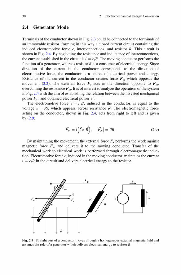
2.4 Generator Mode
Terminals of the conductor shown in Fig. 2.3 could be connected to the terminals of
an immovable resistor, forming in this way a closed current circuit containing the
induced electromotive force e, interconnections, and resistor R. This circuit is
shown in Fig. 2.4. By neglecting the resistance and inductance of interconnections,
the current established in the circuit is i ¼ e/R. The moving conductor performs the
function of a generator, whereas resistor R is a consumer of electrical energy. Since
direction of the current in the conductor corresponds to the direction of
electromotive force, the conductor is a source of electrical power and energy.
Existence of the current in the conductor creates force Fm which opposes the
movement (2.2). The external force Fs acts in the direction opposite to Fm,
overcoming the resistance Fm. It is of interest to analyze the operation of the system
in Fig. 2.4 with the aim of establishing the relation between the invested mechanical
power Fsv and obtained electrical power ei.The electromotive force e ¼ lvB, induced in the conductor, is equal to the
voltage u ¼ Ri, which appears across resistance R. The electromagnetic force
acting on the conductor, shown in Fig. 2.4, acts from right to left and is given
by (2.9):
~Fm ¼ i ~l� ~B� �
; ~Fm
�� �� ¼ ilB: (2.9)
By maintaining the movement, the external force Fs performs the work against
magnetic force Fm and delivers it to the moving conductor. Transfer of the
mechanical work to electrical work is performed through electromagnetic induc-
tion. Electromotive force e, induced in the moving conductor, maintains the current
i ¼ e/R in the circuit and delivers electrical energy to the resistor.
Fig. 2.4 Straight part of a conductor moves through a homogeneous external magnetic field and
assumes the role of a generator which delivers electrical energy to resistor R
30 2 Electromechanical Energy Conversion
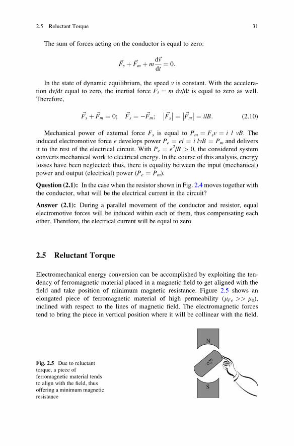
The sum of forces acting on the conductor is equal to zero:
~Fs þ ~Fm þ md~v
dt¼ 0:
In the state of dynamic equilibrium, the speed v is constant. With the accelera-
tion dv/dt equal to zero, the inertial force Fi ¼ m dv/dt is equal to zero as well.
Therefore,
~Fs þ ~Fm ¼ 0; ~Fs ¼ �~Fm; ~Fs
�� �� ¼ ~Fm
�� �� ¼ ilB: (2.10)
Mechanical power of external force Fs is equal to Pm ¼ Fsv ¼ i l vB. Theinduced electromotive force e develops power Pe ¼ ei ¼ i lvB ¼ Pm and delivers
it to the rest of the electrical circuit. With Pe ¼ e2/R > 0, the considered system
converts mechanical work to electrical energy. In the course of this analysis, energy
losses have been neglected; thus, there is equality between the input (mechanical)
power and output (electrical) power (Pe ¼ Pm).
Question (2.1): In the case when the resistor shown in Fig. 2.4 moves together with
the conductor, what will be the electrical current in the circuit?
Answer (2.1): During a parallel movement of the conductor and resistor, equal
electromotive forces will be induced within each of them, thus compensating each
other. Therefore, the electrical current will be equal to zero.
2.5 Reluctant Torque
Electromechanical energy conversion can be accomplished by exploiting the ten-
dency of ferromagnetic material placed in a magnetic field to get aligned with the
field and take position of minimum magnetic resistance. Figure 2.5 shows an
elongated piece of ferromagnetic material of high permeability (mFe >> m0),inclined with respect to the lines of magnetic field. The electromagnetic forces
tend to bring the piece in vertical position where it will be collinear with the field.
Fig. 2.5 Due to reluctant
torque, a piece of
ferromagnetic material tends
to align with the field, thus
offering a minimum magnetic
resistance
2.5 Reluctant Torque 31
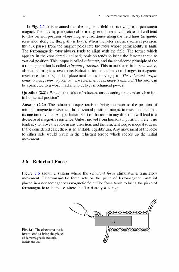
In Fig. 2.5, it is assumed that the magnetic field exists owing to a permanent
magnet. The moving part (rotor) of ferromagnetic material can rotate and will tend
to take vertical position where magnetic resistance along the field lines (magnetic
resistance along the flux path) is lower. When the rotor assumes vertical position,
the flux passes from the magnet poles into the rotor whose permeability is high.
The ferromagnetic rotor always tends to align with the field. The torque which
appears in the considered (inclined) position tends to bring the ferromagnetic to
vertical position. This torque is called reluctant, and the considered principle of thetorque generation is called reluctant principle. This name stems from reluctance,also called magnetic resistance. Reluctant torque depends on changes in magnetic
resistance due to spatial displacement of the moving part. The reluctant torquetends to bring rotor to position where magnetic resistance is minimal. The rotor canbe connected to a work machine to deliver mechanical power.
Question (2.2): What is the value of reluctant torque acting on the rotor when it is
in horizontal position?
Answer (2.2): The reluctant torque tends to bring the rotor to the position of
minimal magnetic resistance. In horizontal position, magnetic resistance assumes
its maximum value. A hypothetical shift of the rotor in any direction will lead to a
decrease of magnetic resistance. Unless moved from horizontal position, there is no
tendency to move the rotor in any direction, and the reluctant torque is equal to zero.
In the considered case, there is an unstable equilibrium. Any movement of the rotor
to either side would result in the reluctant torque which speeds up the initial
movement.
2.6 Reluctant Force
Figure 2.6 shows a system where the reluctant force stimulates a translatory
movement. Electromagnetic force acts on the piece of ferromagnetic material
placed in a nonhomogeneous magnetic field. The force tends to bring the piece of
ferromagnetic to the place where the flux density B is high.
Fig. 2.6 The electromagnetic
forces tend to bring the piece
of ferromagnetic material
inside the coil
32 2 Electromechanical Energy Conversion
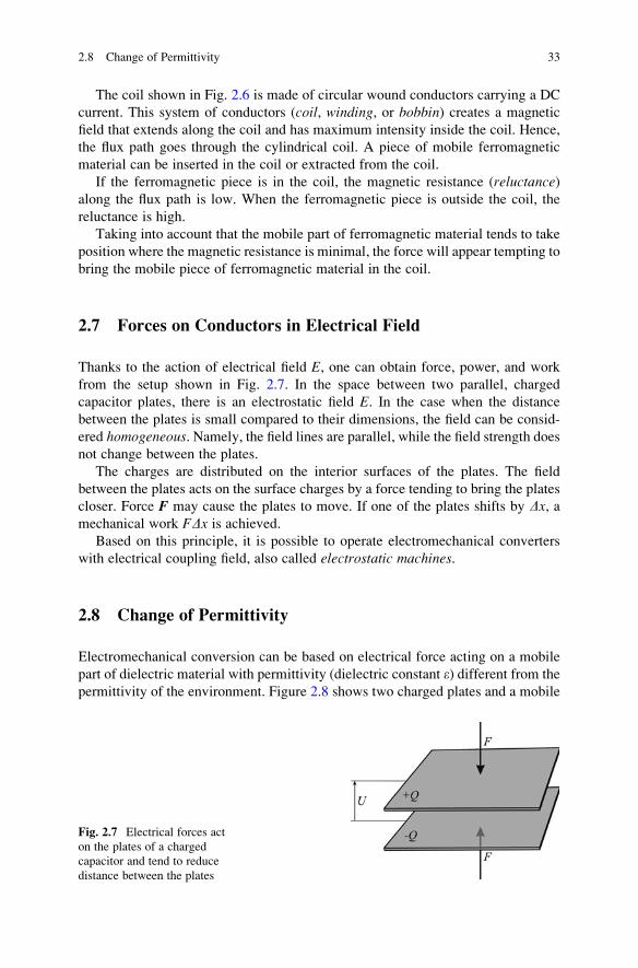
The coil shown in Fig. 2.6 is made of circular wound conductors carrying a DC
current. This system of conductors (coil, winding, or bobbin) creates a magnetic
field that extends along the coil and has maximum intensity inside the coil. Hence,
the flux path goes through the cylindrical coil. A piece of mobile ferromagnetic
material can be inserted in the coil or extracted from the coil.
If the ferromagnetic piece is in the coil, the magnetic resistance (reluctance)along the flux path is low. When the ferromagnetic piece is outside the coil, the
reluctance is high.
Taking into account that the mobile part of ferromagnetic material tends to take
position where the magnetic resistance is minimal, the force will appear tempting to
bring the mobile piece of ferromagnetic material in the coil.
2.7 Forces on Conductors in Electrical Field
Thanks to the action of electrical field E, one can obtain force, power, and work
from the setup shown in Fig. 2.7. In the space between two parallel, charged
capacitor plates, there is an electrostatic field E. In the case when the distance
between the plates is small compared to their dimensions, the field can be consid-
ered homogeneous. Namely, the field lines are parallel, while the field strength does
not change between the plates.
The charges are distributed on the interior surfaces of the plates. The field
between the plates acts on the surface charges by a force tending to bring the plates
closer. Force F may cause the plates to move. If one of the plates shifts by Dx, amechanical work FDx is achieved.
Based on this principle, it is possible to operate electromechanical converters
with electrical coupling field, also called electrostatic machines.
2.8 Change of Permittivity
Electromechanical conversion can be based on electrical force acting on a mobile
part of dielectric material with permittivity (dielectric constant e) different from the
permittivity of the environment. Figure 2.8 shows two charged plates and a mobile
Fig. 2.7 Electrical forces act
on the plates of a charged
capacitor and tend to reduce
distance between the plates
2.8 Change of Permittivity 33
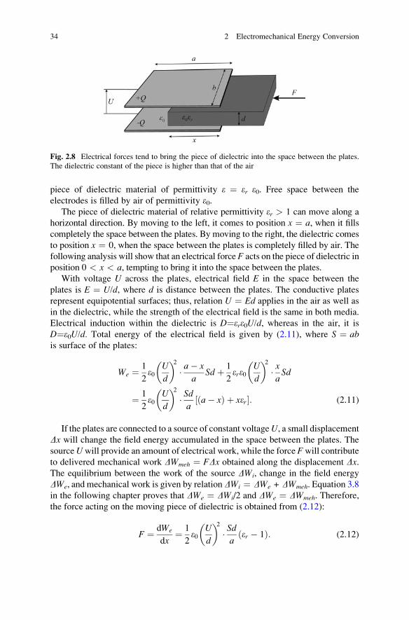
piece of dielectric material of permittivity e ¼ er e0. Free space between the
electrodes is filled by air of permittivity e0.The piece of dielectric material of relative permittivity er > 1 can move along a
horizontal direction. By moving to the left, it comes to position x ¼ a, when it fills
completely the space between the plates. By moving to the right, the dielectric comes
to position x ¼ 0, when the space between the plates is completely filled by air. The
following analysis will show that an electrical force F acts on the piece of dielectric in
position 0 < x < a, tempting to bring it into the space between the plates.
With voltage U across the plates, electrical field E in the space between the
plates is E ¼ U/d, where d is distance between the plates. The conductive plates
represent equipotential surfaces; thus, relation U ¼ Ed applies in the air as well as
in the dielectric, while the strength of the electrical field is the same in both media.
Electrical induction within the dielectric is D¼ere0U/d, whereas in the air, it is
D¼e0U/d. Total energy of the electrical field is given by (2.11), where S ¼ abis surface of the plates:
We ¼ 1
2e0
U
d
� �2� a� x
aSd þ 1
2ere0
U
d
� �2� xaSd
¼ 1
2e0
U
d
� �2� Sda
a� xð Þ þ xer½ �: (2.11)
If the plates are connected to a source of constant voltageU, a small displacement
Dx will change the field energy accumulated in the space between the plates. The
sourceUwill provide an amount of electrical work, while the force Fwill contribute
to delivered mechanical work DWmeh ¼ FDx obtained along the displacement Dx.The equilibrium between the work of the source DWi, change in the field energy
DWe, and mechanical work is given by relation DWi ¼ DWe + DWmeh. Equation 3.8
in the following chapter proves that DWe ¼ DWi/2 and DWe ¼ DWmeh. Therefore,
the force acting on the moving piece of dielectric is obtained from (2.12):
F ¼ dWe
dx¼ 1
2e0
U
d
� �2� Sda
er � 1ð Þ: (2.12)
Fig. 2.8 Electrical forces tend to bring the piece of dielectric into the space between the plates.
The dielectric constant of the piece is higher than that of the air
34 2 Electromechanical Energy Conversion
It is possible to determine electrical force F by using the equivalent pressure on
the surfaces separating the media of different nature. On the basis of a conclusion
from electrostatics, electrical force acting on a dividing surface that separates the
spaces filled with two different dielectric materials can be determined from
the equivalent pressure p ¼ we1 � we2. The values we1 and we2 are specific
energies of electrostatic fields in the two separated media. They are also called
the spatial energy densities of the electrostatic field. The energy of electrical field
energy in the air has density of w0 ¼ ½ e0(U/d)2, whereas in the dielectric it is
wd ¼ ½ ere0(U/d)2. The force F can be determined from (2.13), where Sd ¼ bd ¼
Sd/a is rectangular surface separating the two domains:
F ¼ wd � w0ð ÞSd ¼ 1
2e0
U
d
� �2� er � 1ð Þ � Sd
a: (2.13)
Question (2.3): Determine the direction of force when the source is disconnected.
It should be noted that total chargeQ existing on the plates is then constant, whereas
the voltage between the plates is variable depending on position of the dielectric.
Answer (2.3): In the space between the plates, there is a homogeneous electrical
field. Conductivity 1/r of the metal plates is very high, and potential of all the points
on one plate is the same. Therefore, voltage between the plates is U in the part filled
by the dielectric as well as in the part filled by air. Since the field is homogeneous
and orthogonal to the plates, product Ed is equal to voltage U; thus, electrical fieldE ¼ U/d is the same in both air and the dielectric. Since permittivity of the
dielectric is higher, electrical induction Dd in the dielectric is higher than induction
D0 in the air:
D0 ¼ e0U
d; Dd ¼ ere0
U
d:
Surface charge density s at the surface of a conductor is determined by the scalar
product of the vector of electrical induction and normal to the surface at a given point:
s ¼ ~n � ~D:
In the case being considered, the vector of electrical induction is perpendicular
to the surface of the conductor and collinear with the normal n. As a consequence,the density of surface charge s is equal to the induction D. Therefore, it will behigher in the parts of the plates which are against the dielectric. By using notation
shown in Fig. 2.8, total charge Q can be expressed in terms of the shift x and valuesDd and D0,
Q ¼ a� xð Þb � D0 þ xb � Dd ¼ a� xð Þb � e0 Udþ xb � ere0 U
d
¼ be0U
da� xþ x � erð Þ ;
2.8 Change of Permittivity 35
while capacitance C is determined by expression
C ¼ Q
U¼ be0
da� xþ x � erð Þ:
Since the plates are separated from the source, the mechanical work DWmeh ¼FDx is obtained by subtracting this amount from the field energy, DWmeh ¼ �DWe.
Therefore, the electrical force can be determined according to expression F ¼�dWe/dx. Electrical energy of the coupling field can be expressed as We ¼ ½Q2/Cor We ¼ ½CU2. In the present case, charge Q is constant, whereas voltage U is
variable, and the electrical force can be determined according to expression
F ¼ � dWe
dx¼ �Q2
2
d
dx
1
C
� �:
By differentiating the reciprocal value of capacitance, the following expression
for the electrical force is obtained:
F ¼ � Q2d
2be0
d
dx
1
a� xþ x � er
� �¼ Q2d
2be0er � 1ð Þ 1
a� xþ x � er
� �2:
The above expression is positive, so the direction of action of the force is the
same as if the source was connected to the plates. By introducing substitution
Q ¼ CU in the above expression, the electrical force is determined by
F ¼ U2
2ðer � 1Þ be0
d¼ e0
2
U2
d2ðer � 1Þ Sd
a;
the expression which is fully equivalent to (2.12) and (2.13). It can be concluded
that the force will not change by switching the source on or off, provided that the
charge Q is the same in both cases.
Question (2.4): Consider a charged capacitor made of the plates shown in Fig. 2.8
and assume that the plates are not connected to the source. Is there any difference
between E and D in the part filled by air and part filled by dielectric? Will the total
energy be increased or decreased in the case that the dielectric is pushed further into
the space between the plates?
Answer (2.4): In the space between the plates, the electrical field E is equal in all
points, whereas the electrical induction D is er times higher in the space filled by
dielectric compared to induction in the space filled by air. The spatial density of
the field energy in the dielectric is wed ¼ ½ere0E2, and it is er times higher than the
density wea ¼ ½e0E2 in the air. Total field energy is weaVa + wedVd, where wea and
wed are the densities of field energy in the air and in the dielectric, whereas Va
and Vd are the volumes of the interelectrode space filled by air and dielectric.
36 2 Electromechanical Energy Conversion
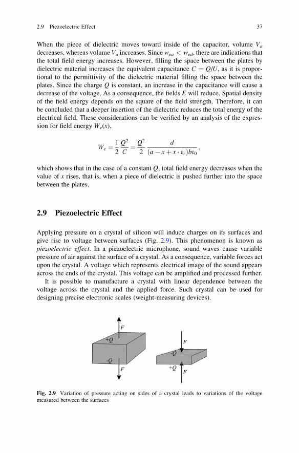
When the piece of dielectric moves toward inside of the capacitor, volume Va
decreases, whereas volume Vd increases. Since wea < wed, there are indications that
the total field energy increases. However, filling the space between the plates by
dielectric material increases the equivalent capacitance C ¼ Q/U, as it is propor-tional to the permittivity of the dielectric material filling the space between the
plates. Since the charge Q is constant, an increase in the capacitance will cause a
decrease of the voltage. As a consequence, the fields E will reduce. Spatial density
of the field energy depends on the square of the field strength. Therefore, it can
be concluded that a deeper insertion of the dielectric reduces the total energy of the
electrical field. These considerations can be verified by an analysis of the expres-
sion for field energy We(x),
We ¼ 1
2
Q2
C¼ Q2
2
d
a� xþ x � erð Þbe0 ;
which shows that in the case of a constant Q, total field energy decreases when the
value of x rises, that is, when a piece of dielectric is pushed further into the space
between the plates.
2.9 Piezoelectric Effect
Applying pressure on a crystal of silicon will induce charges on its surfaces and
give rise to voltage between surfaces (Fig. 2.9). This phenomenon is known as
piezoelectric effect. In a piezoelectric microphone, sound waves cause variable
pressure of air against the surface of a crystal. As a consequence, variable forces act
upon the crystal. A voltage which represents electrical image of the sound appears
across the ends of the crystal. This voltage can be amplified and processed further.
It is possible to manufacture a crystal with linear dependence between the
voltage across the crystal and the applied force. Such crystal can be used for
designing precise electronic scales (weight-measuring devices).
Fig. 2.9 Variation of pressure acting on sides of a crystal leads to variations of the voltage
measured between the surfaces
2.9 Piezoelectric Effect 37
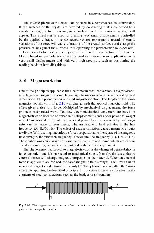
The inverse piezoelectric effect can be used in electromechanical conversion.
If the surfaces of the crystal are covered by conducting plates connected to a
variable voltage, a force varying in accordance with the variable voltage will
appear. This effect can be used for creating very small displacements controlled
by the applied voltage. If the connected voltage represents a record of sound,
variations of the force will cause vibrations of the crystal surfaces and change the
pressure of air against the surfaces, thus operating the piezoelectric loudspeakers.
In a piezoelectric device, the crystal surface moves by a fraction of millimeter.
Motors based on piezoelectric effect are used in motion control applications with
very small displacements and with very high precision, such as positioning the
reading heads in hard disk drives.
2.10 Magnetostriction
One of the principles applicable for electromechanical conversion is magnetostric-tion. In general, magnetization of ferromagnetic materials can change their shape and
dimensions. This phenomenon is called magnetostriction. The length of the ferro-
magnetic rod shown in Fig. 2.10 will change with the applied magnetic field. The
effect gives a rise to a force. Multiplied by mechanical displacement, the force
produces mechanical work. Yet, few electromechanical converters are based on
magnetostriction because of rather small displacements and a poor power-to-weight
ratio. Conventional electrical machines and power transformers usually have mag-
netic circuits made of iron sheets, wherein magnetic field pulsates at the line
frequency (50 Hz/60 Hz). The effect of magnetostriction causes magnetic circuits
to vibrate.With themagnetostrictive forces proportional to the square of themagnetic
field strength, the vibration frequency is twice the line frequency (100 Hz/120 Hz).
These vibrations cause waves of variable air pressure and sound which are experi-
enced as humming, frequently encountered with electrical equipment.
The phenomenon reciprocal to magnetostriction is the change of permeability in
ferromagnetic materials subjected to mechanical stress. Namely, the stress due to
external forces will change magnetic properties of the material. When an external
force is applied to an iron rod, the same magnetic field strength H will result in an
increased magnetic induction (flux density) B. This phenomenon is called the Villarieffect. By applying the described principle, it is possible to measure the stress in the
elements of steel constructions such as the bridges or skyscrapers.
Fig. 2.10 The magnetization varies as a function of force which tends to constrict or stretch a
piece of ferromagnetic material
38 2 Electromechanical Energy Conversion
This chapter discussed the principles of developing electromagnetic forces that
act on moving parts of electromechanical converters and provide the means for the
process of electromechanical conversion. The following chapter introduces some
basic principles of electromechanical converters with electrical coupling field and
electromechanical converters with magnetic coupling field.
2.10 Magnetostriction 39
Chapter 3
Magnetic and Electrical Coupling Field
Electromechanical conversion is based on forces and torques of electromagnetic
origin. The force exerted upon a moving part can be the consequence of electrical or
magnetic field. The field encircles and couples both moving and nonmoving parts of
electromechanical converter. Therefore, the field is also called coupling field. In this
chapter, some basic notions are given for electromechanical energy converters with
electrical coupling field and converters with magnetic coupling field.
3.1 Converters Based on Electrostatic Field
Electromechanical conversion in electrostatic machines is based on electrical
coupling field. The coupling field between moving parts is a prerequisite for electro-
mechanical conversion. In an electrostatic machine, the field exists in the medium
between mobile electrodes, and it causes electrical forces acting on the electrodes.
Preliminary insight in electromechanical energy conversion based on the electrical
field can be obtained by considering the sample machine shown in Fig. 3.1, resem-
bling the capacitor with two parallel metal plates. In the case when the plates are
considerably larger compared to the distance between them (S >> d2), the electricalfield between the electrodes is homogeneous and equal to E ¼ U/d [V/m], where
U is the voltage between the electrodes. Electrical induction vector D [As/m2]
is obtained by multiplying the vector of electric field E by the permittivity of
the medium e0. The force acting on the plates depends on the charge stored in the
capacitor. If it is possible to move one of the plates, then the product of this force and
the displacement gives mechanical work. The mechanical work can be obtained at
the expense of the field energy or of energy of a source connected to the plates.
S.N. Vukosavic, Electrical Machines, Power Electronics and Power Systems,
DOI 10.1007/978-1-4614-0400-2_3, # Springer Science+Business Media New York 2013
41
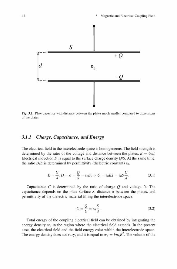
3.1.1 Charge, Capacitance, and Energy
The electrical field in the interelectrode space is homogeneous. The field strength is
determined by the ratio of the voltage and distance between the plates, E ¼ U/d.Electrical induction D is equal to the surface charge density Q/S. At the same time,
the ratio D/E is determined by permittivity (dielectric constant) e0.
E ¼ U
d;D ¼ s ¼ Q
S¼ e0E;) Q ¼ e0ES ¼ e0S
U
d: (3.1)
Capacitance C is determined by the ratio of charge Q and voltage U. Thecapacitance depends on the plate surface S, distance d between the plates, and
permittivity of the dielectric material filling the interelectrode space:
C ¼ Q
U¼ e0
S
d: (3.2)
Total energy of the coupling electrical field can be obtained by integrating the
energy density we in the region where the electrical field extends. In the present
case, the electrical field and the field energy exist within the interelectrode space.
The energy density does not vary, and it is equal to we ¼ ½e0E2. The volume of the
Fig. 3.1 Plate capacitor with distance between the plates much smaller compared to dimensions
of the plates
42 3 Magnetic and Electrical Coupling Field
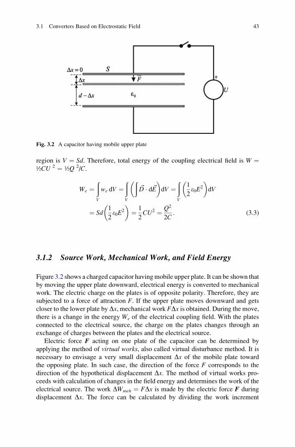
region is V ¼ Sd. Therefore, total energy of the coupling electrical field is W ¼½CU 2 ¼ ½Q 2/C.
We ¼ðV
we dV ¼ðV
ð~D � d~E
� �dV ¼
ðV
1
2e0E2
� �dV
¼ Sd1
2e0E2
� �¼ 1
2CU2 ¼ Q2
2C: (3.3)
3.1.2 Source Work, Mechanical Work, and Field Energy
Figure 3.2 shows a charged capacitor havingmobile upper plate. It can be shown that
by moving the upper plate downward, electrical energy is converted to mechanical
work. The electric charge on the plates is of opposite polarity. Therefore, they are
subjected to a force of attraction F. If the upper plate moves downward and gets
closer to the lower plate by Dx, mechanical work FDx is obtained. During the move,
there is a change in the energy We of the electrical coupling field. With the plates
connected to the electrical source, the charge on the plates changes through an
exchange of charges between the plates and the electrical source.
Electric force F acting on one plate of the capacitor can be determined by
applying the method of virtual works, also called virtual disturbance method. It is
necessary to envisage a very small displacement Dx of the mobile plate toward
the opposing plate. In such case, the direction of the force F corresponds to the
direction of the hypothetical displacement Dx. The method of virtual works pro-
ceeds with calculation of changes in the field energy and determines the work of the
electrical source. The work DWmeh ¼ FDx is made by the electric force F during
displacement Dx. The force can be calculated by dividing the work increment
Fig. 3.2 A capacitor having mobile upper plate
3.1 Converters Based on Electrostatic Field 43
DWmeh by the displacement Dx. The same virtual work method can be applied in
cases when the mobile part of the electromechanical converter performs rotation.
In such cases, the displacement Dx is replaced by the angular shift Dy, while the
mechanical works DWmeh assume the form TemDy. The symbol Tem designates
the torque generated by the electrical forces. The torque Tem acts upon the moving
(revolving) part and affects its speed.
A source of the constant voltage U, shown on the right-hand side of Fig. 3.2, canbe connected to the plates by closing the switch. Reduction of the distance d betweenthe plates increases capacitance C. While the source is connected, the voltage
between the plates is constant. Due to an increase of the capacitance, the charge
on the plates Q ¼ CU increases. Therefore, the source supplies an additional
charge DQ. The work of the source is equal to DWi ¼ UDQ, while the obtained
mechanical work is DWmeh ¼ FDx. The work of the source increases total energy ofthe system, that is, the sum of the electrical energy and mechanical work. With a
constant voltage, the electrical energy is given by (3.4).
In the next considerations, it will be shown that work of the source is divided in
two equal parts, that is, DWe ¼ DWmeh ¼ ½DWi.
If the switch in Fig. 3.2 is open, the source is separated from the plates, and the
work of the source is equal to zero. Electrical charges on the plates cannot be
changed, as well as the field D between the plates (Q ¼ const., D ¼ const.).
Therefore, the density of the field energy we ¼ ½D2/e0 remains unchanged.
By reducing the distance between the plates, the volume of the region compris-
ing the electrical field is reduced as well. Therefore, the total field energy DWe is
also reduced. With the source separated from the system, reduction in the field
energy yields the mechanical work DWmeh ¼ �DWe. In the case of a constant
charge, the field electrical energy is given by (3.5):
We Dxð Þ ¼ S d � Dxð Þ 1
2e0E2
� �¼ 1
2CU2 ¼ U2
2
e0Sd � Dx
; (3.4)
We Dxð Þ ¼ S d � Dxð Þ 1
2e0E2
� �¼ Q2
2C¼ Q2
2
d � Dxe0S
: (3.5)
3.1.3 Force Expression
The machines operating with the electrical coupling field are called electrostatic
machines. Domain with the electrical field is filled with dielectric material. Dielec-
tric is called linear if the vector of electrical inductionD is proportional to the vector
E, D ¼ eE. Electrostatic machine with linear dielectric is called linear machine.The structure shown in Fig. 3.2 represents a linear electrostatic machine with
negligible energy losses. Therefore, in the case with Q ¼ const., the mechanical
44 3 Magnetic and Electrical Coupling Field
work DWmeh ¼ FDx is determined by DWmeh ¼ �DWe, whereas in the case of a
constant voltage relation, DWmeh ¼ +DWe ¼ +½DWi applies. According to these
expressions, the force can be determined as partial derivative of the coupling field
energy We with respect to coordinate x. This coordinate represents displacement of
the mobile electrode along the motion axis of the system.
In the case when the source is disconnected, the system in Fig. 3.2 has a constant
charge, and the work of the source U is equal to zero. Applying the method of
virtual works, the change in the field energy and the mechanical work are obtained
from (3.6).
DWi ¼ UDQ ¼ 0
DWi ¼ DWmeh þ DWe ) DWmeh ¼ �DWe: (3.6)
When the source is disconnected, the force F acting on the mobile electrode is
given by (3.7). In the case when the changes DWe and Dx are very small, the ratio
DWe/Dx assumes the value of the first derivative of We(x),
F ¼ �DWe
Dx;
F ¼ � dWe
dx¼ � d
dx
Q2
2
d � x
e0S
� �¼ Q2
2Se0: (3.7)
If the source is connected, the considered system has a constant voltage. By
applying the method of virtual works, the work of the source U, the change in the
field energy, and the mechanical work are obtained in (3.8):
DWi ¼ U DQ; DWe ¼ DCU2
2
� �¼ 1
2UDQ ¼ 1
2DWi;
DWi ¼ DWmeh þ DWe ) DWmeh ¼ DWi � DWe ¼ DWe: (3.8)
With the source connected, the force F acting on the mobile electrode is given by
(3.9). With infinitesimally small changes DWe and Dx, the ratio DWe/Dx assumes
the value of the first derivative dWe (x)/dx,
F ¼ þ dWe
dx¼ d
dx
U2
2
e0Sd � x
� �¼ U2
2
e0S
d � xð Þ2
¼ E2
2e0S ¼ D2
2e0S ¼ Q2
2Se0: (3.9)
Expressions for electrical force, given by (3.7) and (3.9), are applicable only
when the medium is linear, that is, when the permittivity of the dielectric material
does not depend on the field strength. In cases when the source U is not connected,
displacement of the mobile electrode does not cause any change in charge Q.
3.1 Converters Based on Electrostatic Field 45
Instead, it leads to changes in the capacitance C and the voltage across the plates.
The expression for electrical force when the source is disconnected takes the
following form:
F ¼ � dWe
dx¼ � d
dx
Q2
2
1
C
� �¼ �Q2
2
d
dx
1
C
� �:
If the source is connected, the voltage across the plates is constant. Therefore,
the shift of the mobile electrode changes the capacitance C and the charge Q. Theforce expression assumes the following form:
F ¼ þ dWe
dx¼ þ d
dx
U2
2C
� �¼ þU2
2
dC
dx:
Question (3.1): Equation 3.7 gives force F acting on the mobile electrode in the
case when the source is disconnected, whereas (3.9) gives this force when the source
is connected. Note that in both cases, the same result is obtained, proportional toQ2.
Is it possible that the force acting on the mobile electrode does depend on source Ubeing connected or disconnected? Provide an explanation.
Answer (3.1): The electrical force acting on the mobile plate can be represented as
a sum of forces acting on electrical charges distributed over the plate surface.
Individual forces are dependent on the density of electrical charge and the field
strength in the vicinity of the plate. It is necessary to compare the force obtained
with the source U connected to the force obtained with the source detached from
the plates. If the plates accommodate the same electrical charge Q in both cases, the
surface charge density remains the same. The surface charge density determines
the electrical induction D. Therefore, in both cases, the electrical field strength
E ¼ D/e0 is the same. From this, it can be concluded that in both cases the same
force acts on the mobile plate.
3.1.4 Conversion Cycle
In the preceding section, it has been shown that the electromechanical conversion
can be performed in two different modes. With the source disconnected, mechani-
cal work DWmeh is obtained on account of the energy accumulated in the coupling
field, DWmeh ¼ �DWe. If the source is connected, the work of the source DWi is
divided in two equal parts, that is, DWe ¼ DWmeh ¼ ½ DWi. Graphical representa-
tion of electromechanical conversion is shown in Fig. 3.3. It is of interest to note
that none of the two presented modes can last continuously.
If the source is connected, the electromechanical conversion is performed by
turning one part of the source work into mechanical energy, whereas the rest of the
46 3 Magnetic and Electrical Coupling Field
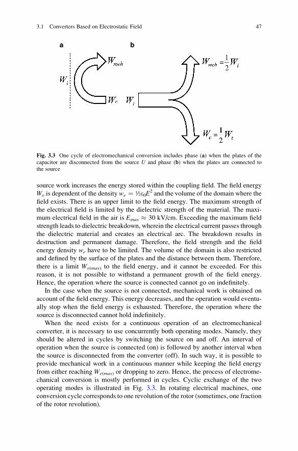
source work increases the energy stored within the coupling field. The field energy
We is dependent of the density we ¼ ½e0E2 and the volume of the domain where the
field exists. There is an upper limit to the field energy. The maximum strength of
the electrical field is limited by the dielectric strength of the material. The maxi-
mum electrical field in the air is Emax � 30 kV/cm. Exceeding the maximum field
strength leads to dielectric breakdown, wherein the electrical current passes through
the dielectric material and creates an electrical arc. The breakdown results in
destruction and permanent damage. Therefore, the field strength and the field
energy density we have to be limited. The volume of the domain is also restricted
and defined by the surface of the plates and the distance between them. Therefore,
there is a limit We(max) to the field energy, and it cannot be exceeded. For this
reason, it is not possible to withstand a permanent growth of the field energy.
Hence, the operation where the source is connected cannot go on indefinitely.
In the case when the source is not connected, mechanical work is obtained on
account of the field energy. This energy decreases, and the operation would eventu-
ally stop when the field energy is exhausted. Therefore, the operation where the
source is disconnected cannot hold indefinitely.
When the need exists for a continuous operation of an electromechanical
converter, it is necessary to use concurrently both operating modes. Namely, they
should be altered in cycles by switching the source on and off. An interval of
operation when the source is connected (on) is followed by another interval when
the source is disconnected from the converter (off). In such way, it is possible to
provide mechanical work in a continuous manner while keeping the field energy
from either reaching We(max) or dropping to zero. Hence, the process of electrome-
chanical conversion is mostly performed in cycles. Cyclic exchange of the two
operating modes is illustrated in Fig. 3.3. In rotating electrical machines, one
conversion cycle corresponds to one revolution of the rotor (sometimes, one fraction
of the rotor revolution).
Fig. 3.3 One cycle of electromechanical conversion includes phase (a) when the plates of the
capacitor are disconnected from the source U and phase (b) when the plates are connected to
the source
3.1 Converters Based on Electrostatic Field 47
Question (3.2): Estimate the mechanical work obtained during one cycle with
electromechanical converter made of a plate capacitor with one mobile plate.
The dimensions of the plates and minimum and maximum distances between the
plates are known, while the maximum electrical field strength in the dielectric is
Emax ¼ 30 kV/cm.
Answer (3.2): The maximum work obtainable in one cycle is determined by the
maximum energy of the coupling field. The surface of the plates S, maximum
distance between the plates d, and maximum energy density of the coupling field
we ¼ ½e0Em2 are known. The mechanical work which can be obtained within one
cycle is DW ¼ S d we(max).
Question (3.3): If a converter makes f cycles per second, estimate its average
power.
Answer (3.3): Average power of the converter making f cycles per second is
Pa v ¼ fDW ¼ f S d we(max).
3.1.5 Energy Density of Electrical and Magnetic Field
The power of an electromechanical converter is dependent on the density of energy
accumulated within the coupling field. A converter of given dimensions will have
higher average power if its coupling field has a higher energy density. Given the
converter power, dimensions and mass will be reduced for an increased density of
energy. The power-to-size ratio is also called specific power. The considerations
which follow show that electromechanical converters involving magnetic coupling
field possess higher specific power compared to electrostatic machines.
Themechanical work obtained within one cycle of electromechanical converter is
dependent on the energy stored in the coupling field. The maximum amount of the
field energy is dependent on the energy density and the volume of the converter.
If two electrical machines of the same size are considered, the machine with higher
density of the field energy will produce higher mechanical work within each conver-
sion cycle. If the repetition rates of conversion cycles are the same for the two
machines, themachine having higher energy density will have higher average power.
The energy density of magnetic field exceeds by large the density of energy in
electrical field. Permittivity (D/E) in vacuum is e0 ¼ 8.85�10�12 � 10�11, whereas
permeability (B/H) amounts m0 ¼ 4p�10�7 � 10�6. Therefore, the energy density
of magnetic field wm ¼ m0H2/2 is considerably higher than the energy density of
electrical field we ¼ e0E2/2. For this reason, electrical machines are mostly
operating with magnetic coupling field.
Density of energy accumulated in the coupling field depends on the square of the
field strength. In air, electrical field is limited by dielectric strength, Emax � 30
kV/cm � 3MV/m. In electrical machines with magnetic field, the field is comprised
by magnetic circuit including air gaps and ferromagnetic materials such as iron.
48 3 Magnetic and Electrical Coupling Field
Magnetic inductance B in ferromagnetic materials is limited to Bmax ¼ 1–2 T, thus
limiting the magnetic inductance achievable in air. Consequently, the maximum
field strength H which can be met in electrical machines is close to Hmax � Bmax/
m0 � 1 MA/m. With e0 � 10�11 and m0 � 10�6, the achievable energy density is
much higher in the case of magnetic field. Considering two electromechanical
converters of the same size, the converter operating with magnetic field could
accumulate much higher energy in the coupling field (103–104 times) and propor-
tionally higher average power of electromechanical conversion.
3.1.6 Coupling Field and Transfer of Energy
It is of interest to note that both the electromechanical energy conversion with
magnetic coupling field and the conversion with electrical field involve both field
vectors, electrical field vector E and magnetic field vector H. The exchange of
energy between electrical and mechanical terminals of electrical machine implies
that in the space surrounding the moving part of the machine, there is transfer of
energy toward the moving part (motor) or from the moving part (generator). The
energy transfer through the surrounding space is measured by Poynting vector.Hence, the energy streams through domain if the Poynting vector has a nonzero
algebraic intensity. Poynting vector is equal to the vector product of the electrical
and magnetic field. It represents the surface density of power, and it is expressed in
W/m2. Surface integral of Poynting vector over a surface separating two domains
represents the rate of energy transfer from one to the other domain (i.e., the power
passed from one domain to another). The course and direction of Poynting vector
indicate the course and direction of energy transfer. In the absence of either
electrical field E or magnetic field H, Poynting vector is equal to zero; thus, no
energy transfer is possible. Therefrom, the question arises on how do electrical
machines with electrical coupling field acquire magnetic field H required for
mandatory Poynting vector.
In an electromechanical converter involving electrical coupling field which is at
the state of rest, the magnetic field will be equal to zero and so will be Poynting
vector. This is an expected situation since the power of electromechanical conver-
sion is zero in the case when mobile parts of the converter do not move. Namely, the
power is equal to the product of the force and speed of motion. At rest, although
the electrical force may be present, the speed is equal to zero, thus resulting in zero
mechanical power. If the considered converter is in the state of motion, its mobile
part moves in the electrical coupling field. This leads to variations in the field
strength E and the electrical induction D within the converter. The first time
derivative of D contributes to the spatial derivative (i.e., curl) of magnetic field H.The second Maxwell equation expresses generalized Ampere law, and it reads
rot ~H ¼ ~J þ @~D
@t: (3.10)
3.1 Converters Based on Electrostatic Field 49
Since a nonzero spatial derivative of the field H exists, algebraic intensity of
the vector H cannot be equal to zero at all points of the considered domain. The
conclusion is that a certain magnetic field H exists in electrostatic machines in
the state of motion. The field strength H is proportional to the speed of the machine
moving parts. In conjunction with the field E, magnetic field H results in Poynting
vector P ¼ E � H.
The same considerations can be derived for an electromechanical converter
based on magnetic coupling field. At rest, the magnetic field H exists in the
converter, but the electrical field E and Poynting vector P are equal to zero. With
P ¼ 0, there is no flow of energy toward the mobile part of the machine, and the
mechanical power is equal to zero. This corresponds to the conclusion that
the mechanical power at rest must be zero, as it is the product of the force and
the speed. When the considered converter is in the state of motion, its mobile parts
move in the magnetic coupling field. This leads to variations in the magnetic field
H and the magnetic induction B within the converter. The first Maxwell equation
expresses the Faraday law in differential form, and it reads
rot ~E ¼ � @~B
@t: (3.11)
Hence, the variation of magnetic induction B results in the spatial derivative
(curl) of electrical field, which causes the appearance of the electrical field E within
the converter and leads to nonzero values of the Poynting vector.
3.2 Converter Involving Magnetic Coupling Field
Electromechanical conversion in converters involving magnetic coupling field is
possible by means of the field acting on the mobile windings and mobile parts made
of ferromagnetic materials. In such converters, magnetic field is a precondition for
electromechanical conversion of energy. It exists in the space between the station-
ary and mobile parts of magnetic circuits and current circuits. The mobile parts can
perform either linear or rotational movement.
Forces acting on mobile parts are dependent on the magnetic induction and
current in conductors. Mechanical work can be obtained on account of the field
energy or work of the source which is connected to the current carrying conductors.
3.2.1 Linear Converter
Figure 3.4 shows a simple electromechanical converter involving homogeneous
magnetic field and a straight part of the conductor performing linear motion.
The subsequent analysis is focused on motoring operation of the converter, wherein
50 3 Magnetic and Electrical Coupling Field
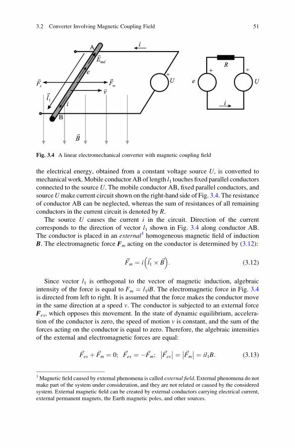
the electrical energy, obtained from a constant voltage source U, is converted to
mechanical work.Mobile conductor AB of length l1 touches fixed parallel conductorsconnected to the source U. The mobile conductor AB, fixed parallel conductors, and
sourceUmake current circuit shown on the right-hand side of Fig. 3.4. The resistance
of conductor AB can be neglected, whereas the sum of resistances of all remaining
conductors in the current circuit is denoted by R.The source U causes the current i in the circuit. Direction of the current
corresponds to the direction of vector l1 shown in Fig. 3.4 along conductor AB.
The conductor is placed in an external1 homogeneous magnetic field of induction
B. The electromagnetic force Fm acting on the conductor is determined by (3.12):
~Fm ¼ i ~l1 � ~B� �
: (3.12)
Since vector l1 is orthogonal to the vector of magnetic induction, algebraic
intensity of the force is equal to Fm ¼ l1iB. The electromagnetic force in Fig. 3.4
is directed from left to right. It is assumed that the force makes the conductor move
in the same direction at a speed v. The conductor is subjected to an external force
Fex, which opposes this movement. In the state of dynamic equilibrium, accelera-
tion of the conductor is zero, the speed of motion v is constant, and the sum of the
forces acting on the conductor is equal to zero. Therefore, the algebraic intensities
of the external and electromagnetic forces are equal:
~Fex þ ~Fm ¼ 0; ~Fex ¼ �~Fm; ~Fex
�� �� ¼ ~Fm
�� �� ¼ il1B: (3.13)
Fig. 3.4 A linear electromechanical converter with magnetic coupling field
1Magnetic field caused by external phenomena is called external field. External phenomena do not
make part of the system under consideration, and they are not related or caused by the considered
system. External magnetic field can be created by external conductors carrying electrical current,
external permanent magnets, the Earth magnetic poles, and other sources.
3.2 Converter Involving Magnetic Coupling Field 51
While the conductor moves in magnetic field, the electromotive force eABis induced between its ends. Electrical field Eind induced in the conductor is
determined by the vector product of the speed v and magnetic induction B. Sincethe vector of the induced field does not vary along the conductor, the electromotive
force e ¼ eAB can be calculated from (3.14):
e ¼ �~l1� �
� ~Eind ¼ �~l1� �
� ~v� ~B
: (3.14)
Vector of the induced electrical field is collinear with the conductor. Therefore,
the electromotive force is equal to e ¼ l1vB. The sign of the induced electromotive
force e ¼ eAB is related to the adopted reference direction, shown in Fig. 3.4.
Positive value of the electromotive force, e ¼ eAB > 0, acts toward increasing
the potential at the conductor end A with respect to the potential at the end B.
Current i ¼ (U � e)/R exists in the circuit shown in the Fig. 3.4. At steady state,
time varying electrical current i(t) assumes a constant value I ¼ (U � l1vB)/R.Power of the source Pi ¼ Ui ¼ ei + Ri2 contains the component PAB ¼ ei ¼ l1vBas well as the losses Pg¼Ri2. The losses in conductors are caused by Joule effect, andthey depend on the equivalent resistance and square of the current. The remaining
power PAB is transferred to the moving conductor. By maintaining the movement,
electromagnetic force Fm performs the work against external force Fex which is
opposite to motion. Vectors of the force and speed of motion are collinear. There-
fore, the mechanical power is equal to Pmeh ¼ Fmv ¼ l1ivB. Power Pmeh is the
output power of the electromechanical converter which converts electrical energy
obtained from the source U to mechanical work. Since Pmeh ¼ Fmv ¼ PAB ¼ ei ¼l1vBi, distribution of the source power Pi can be described by expression
Pi ¼ Ui ¼ eiþ Ri2 ¼ Fmvþ Ri2 ¼ Pmeh þ Ri2: (3.15)
Therefore, power from the source is divided in the thermal losses and mechanical
power, the latter being the result of electromechanical conversion. The power
delivered by the induced electromotive force e is equal to Pe ¼ e(�i) ¼ �ei < 0.
Consequently, the electromotive force e behaves as a receiver, taking over the
electrical power ei ¼ l1vBi which is then converted to mechanical power Pmeh ¼Fmv ¼ ei. In the presented example, the mechanical power of the electromechanical
converter is equal to the product of the electromotive force and current. Equa-
tion 3.16 in certain form is present in all electrical machines:
ei ¼ Fmv: (3.16)
Joule losses are determined by the power Pg ¼ Ri2, and they are turned into heat.Conductors and other parts of the converter are heated. Compared to ambient
temperature, their temperatures are increased. Due to elevated temperatures, these
parts of the converter transfer their heat to the ambient by convection, conduction,
or radiation. When the power of losses Pg becomes equal to the heat power
transferred to the ambient, the temperature increase stops and the system enters
the thermal equilibrium. Since the electromechanical converters are used for
52 3 Magnetic and Electrical Coupling Field
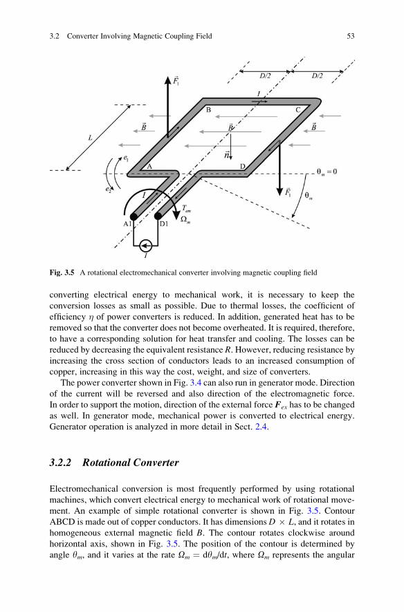
converting electrical energy to mechanical work, it is necessary to keep the
conversion losses as small as possible. Due to thermal losses, the coefficient of
efficiency � of power converters is reduced. In addition, generated heat has to be
removed so that the converter does not become overheated. It is required, therefore,
to have a corresponding solution for heat transfer and cooling. The losses can be
reduced by decreasing the equivalent resistance R. However, reducing resistance byincreasing the cross section of conductors leads to an increased consumption of
copper, increasing in this way the cost, weight, and size of converters.
The power converter shown in Fig. 3.4 can also run in generator mode. Direction
of the current will be reversed and also direction of the electromagnetic force.
In order to support the motion, direction of the external force Fex has to be changed
as well. In generator mode, mechanical power is converted to electrical energy.
Generator operation is analyzed in more detail in Sect. 2.4.
3.2.2 Rotational Converter
Electromechanical conversion is most frequently performed by using rotational
machines, which convert electrical energy to mechanical work of rotational move-
ment. An example of simple rotational converter is shown in Fig. 3.5. Contour
ABCD is made out of copper conductors. It has dimensions D � L, and it rotates inhomogeneous external magnetic field B. The contour rotates clockwise around
horizontal axis, shown in Fig. 3.5. The position of the contour is determined by
angle ym, and it varies at the rate Om ¼ dym/dt, where Om represents the angular
Fig. 3.5 A rotational electromechanical converter involving magnetic coupling field
3.2 Converter Involving Magnetic Coupling Field 53
speed in rad/s. At certain instant, the contour is in position ym ¼ 0, when lines of
the magnetic field are parallel to surface S ¼ D � L, surrounded by the contour.
Terminals of the contour are connected to power supply which provides the current
I in the conductor.
Electromagnetic force F1 acts on parts AB and CD of the conductive contour.
These parts are of length L and are orthogonal to the magnetic field; thus, the force is
determined by expression F1 ¼ LIB. The electromagnetic force does not act on the
transversal parts BC andDAof lengthD, because the current in these parts is collinearwith the magnetic field. At position ym ¼ p/2, the transversal parts BC and DA are
subjected to the actions of forces in the direction of rotation, but the forces are
collinear and of opposite directions; therefore, their actions are mutually canceled.
The couple of electromagnetic forces in Fig. 3.5 creates the torque Tem ¼ DF1.
Assuming that the contour rotates with angular frequency Om ¼ dym/dt, the
developed mechanical power at the considered instant (t ¼ 0, ym ¼ 0) is equal
to Pmeh ¼ TemOm ¼ DLIBOm. Power Pmeh is the output power of the electrome-
chanical converter which converts the electrical energy obtained from the supply Ito mechanical work.
It is of interest to compare the obtained mechanical power with the electrical
power taken from the source. Between terminals A1 and D1 of the constant current
source I, there is voltage u ¼ vA1 � vD1. The source is connected to the contour
ABCD, and the voltage is u ¼ RI + dF/dt, whereF denotes the flux through surface
S encircled by the contour, while R denotes the equivalent resistance of the
conductors making the contour. Reference direction of the flux is the direction of
the positive normal n to surface S. This normal is in accordance with the direction
of circulation along the contour ABCD, that is, the current in designated direction of
circulation along the contour creates a magnetic field which is aligned with the
normal n. In Figs. 3.5 and 3.6, the normal is denoted by vector n. The contour canrotate around horizontal axis; thus, the flux through the surface S depends upon
the angle ym between the vectors of magnetic induction and the plane in which the
surface S reclines.
In accordance with the notation in Fig. 3.6, the angle ym is equal to zero at the
position where the magnetic field is parallel to the surface S. In zero position, fluxFis equal to zero. When the contour makes an angular shift of ym, the normal n to
surface S is shifted to position n1. Assuming that the external field is homogeneous,
F can be represented by the expression F(ym) ¼ Fmsin(ym) ¼ Fmsin(Omt), whereFm ¼ BS is the maximum value of flux which is attained at position ym ¼ p/2. Byusing the obtained expression for the flux, the voltage across the terminals of the
source is calculated as u ¼ RI + OmFmcos(Omt). At position ym ¼ 0, the power
delivered by the source I to the converter is given in (3.17):
Pi ¼ uI ¼ RI2 þ IOmFm ¼ RI2 þ IOmBS
¼ RI2 þ DLIBOm ¼ Pmeh þ RI2: (3.17)
Therefore, the power of the source I is partially converted to mechanical power,
whereas the remaining part accounts for conversion losses that are turned into heat
54 3 Magnetic and Electrical Coupling Field
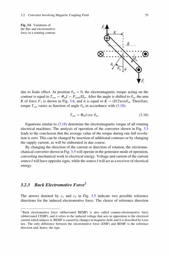
due to Joule effect. At position ym ¼ 0, the electromagnetic torque acting on the
contour is equal to Tem ¼ FmI ¼ Pmeh/Om. After the angle is shifted to ym, the armK of force F1 is shown in Fig. 3.6, and it is equal to K ¼ (D/2)cosym. Therefore,torque Tem varies as function of angle ym in accordance with (3.18):
Tem ¼ FmI cos ym: (3.18)
Equations similar to (3.18) determine the electromagnetic torque of all rotating
electrical machines. The analysis of operation of the converter shown in Fig. 3.5
leads to the conclusion that the average value of the torque during one full revolu-
tion is zero. This can be changed by insertion of additional contours or by changing
the supply current, as will be elaborated in due course.
By changing the direction of the current or direction of rotation, the electrome-
chanical converter shown in Fig. 3.5 will operate in the generator mode of operation,
converting mechanical work to electrical energy. Voltage and current of the current
source Iwill have opposite signs, while the source Iwill act as a receiver of electricalenergy.
3.2.3 Back Electromotive Force2
The arrows denoted by e1 and e2 in Fig. 3.5 indicate two possible reference
directions for the induced electromotive force. The choice of reference direction
Fig. 3.6 Variations of
the flux and electromotive
force in a rotating contour
2 Back electromotive force (abbreviated BEMF) is also called counter-electromotive force
(abbreviated CEMF), and it refers to the induced voltage that acts in opposition to the electrical
current which induces it. BEMF is caused by changes in magnetic field, and it is described by Lenz
law. The only difference between the electromotive force (EMF) and BEMF is the reference
direction and, hence, the sign.
3.2 Converter Involving Magnetic Coupling Field 55
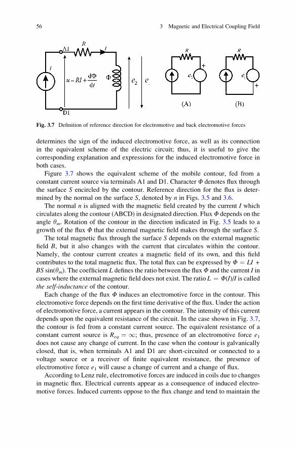
determines the sign of the induced electromotive force, as well as its connection
in the equivalent scheme of the electric circuit; thus, it is useful to give the
corresponding explanation and expressions for the induced electromotive force in
both cases.
Figure 3.7 shows the equivalent scheme of the mobile contour, fed from a
constant current source via terminals A1 and D1. Character F denotes flux through
the surface S encircled by the contour. Reference direction for the flux is deter-
mined by the normal on the surface S, denoted by n in Figs. 3.5 and 3.6.
The normal n is aligned with the magnetic field created by the current I whichcirculates along the contour (ABCD) in designated direction. FluxF depends on the
angle ym. Rotation of the contour in the direction indicated in Fig. 3.5 leads to a
growth of the flux F that the external magnetic field makes through the surface S.The total magnetic flux through the surface S depends on the external magnetic
field B, but it also changes with the current that circulates within the contour.
Namely, the contour current creates a magnetic field of its own, and this field
contributes to the total magnetic flux. The total flux can be expressed by F ¼ LI +BS sin(ym). The coefficient L defines the ratio between the fluxF and the current I incases where the external magnetic field does not exist. The ratio L ¼ F(I)/I is calledthe self-inductance of the contour.
Each change of the flux F induces an electromotive force in the contour. This
electromotive force depends on the first time derivative of the flux. Under the action
of electromotive force, a current appears in the contour. The intensity of this current
depends upon the equivalent resistance of the circuit. In the case shown in Fig. 3.7,
the contour is fed from a constant current source. The equivalent resistance of a
constant current source is Req ¼ 1; thus, presence of an electromotive force e1does not cause any change of current. In the case when the contour is galvanically
closed, that is, when terminals A1 and D1 are short-circuited or connected to a
voltage source or a receiver of finite equivalent resistance, the presence of
electromotive force e1 will cause a change of current and a change of flux.
According to Lenz rule, electromotive forces are induced in coils due to changes
in magnetic flux. Electrical currents appear as a consequence of induced electro-
motive forces. Induced currents oppose to the flux change and tend to maintain the
Fig. 3.7 Definition of reference direction for electromotive and back electromotive forces
56 3 Magnetic and Electrical Coupling Field
initial flux value. Electrical current in a coil creates magnetic field and the flux
which is proportional to the self-inductance of the coil. Direction of this self-flux isopposite to the original flux change. Hence, the induced electromotive force
produces the current and the self-flux in direction that tends to cancel the original
flux change. For that reason, induced electromotive forces are also called counter-electromotive forces or back electromotive forces.
Considering the setup in Fig. 3.5, during rotation of the contour in the direction
indicated in the figure, the flux due to external magnetic field rises. Electromotive
force e1, given by (3.19), appears in the contour:
e1 ¼ � dFdt
: (3.19)
Since an increase of the flux results in e1 < 0, a current appears opposite to
the direction of circulation along the galvanically closed contour ABCD. Therefore,
the induced current creates its own magnetic field and the self-flux of the contour
in the direction opposite to the indicated normal n. Total flux is equal to the sum
of fluxes due to external field, which is growing, and the self-flux which is of nega-
tive sign.
Electromagnetic induction opposes to changes of the flux to the degree which
depends on the circuit parameters. When the equivalent resistance of the circuit is
Req ¼ 1, the induced electromotive force does not cause any change in electrical
current which would have opposed to changes in the flux. In cases when the
equivalent resistance of the contour is zero (Req ¼ 0, the case of a superconductive
contour with short-circuited terminals), the phenomenon of electromagnetic induc-
tion prevents any changes of flux. Since the voltage balance equation is given in
(3.20)
u ¼ Ri� e1 ¼ Riþ dFdt
; (3.20)
in conditions with u ¼ 0 and R ¼ 0, the flux cannot change due to dF/dt ¼ 0.
Therefore, notwithstanding eventual changes in the external magnetic field, the
total flux through a short-circuited superconductive contour is constant.
For a contour fed from a constant current source, shown in Fig. 3.5, the equivalent
schemes of the electrical circuit are shown in Fig. 3.7. For the reference direction of
the induced electromotive force, it is possible to use e1 or e2, as indicated in Figs. 3.5and 3.7. If the reference direction e1 is chosen, the equivalent scheme (B) of Fig. 3.7
applies, and algebraic intensity of the electromotive force is determined by (3.19).
Alternatively, the equivalent scheme (A) and (3.21) apply. Quantity e2 ¼ +dF/dt iscalled back electromotive force or counter-electromotive force:
e2 ¼ �e1 ¼ dFdt
: (3.21)
3.2 Converter Involving Magnetic Coupling Field 57
Chapter 4
Magnetic Circuit
This chapter introduces and explains magnetic circuits of electrical machines. Basic
laws and skills required to analyze magnetic circuits are reinstated and illustrated
on examples and solved problems. The terms such as magnetic resistance, magneto-
motive force, core flux, and winding flux are recalled and applied. Dual electrical
circuit is introduced, explained, and applied in solving magnetic circuits. Basic
properties of ferromagnetic materials are recalled, including saturation phenomena,
eddy current losses, and hysteresis losses. Laminated magnetic circuits as the
means of reducing the iron losses are explained and analyzed.
One of the key operating principles of electromechanical converters based on
magnetic field is creation of Lorentz force acting on a current-carrying conductor
placed in the magnetic field. Magnetic field can be obtained from a permanent
magnet or by using an electromagnet. Electromagnet is a system of windings
carrying electrical currents that create magnetic field. It is useful in replacing the
permanent magnets by coils carrying a relatively small electrical current. For
the electromagnet currents to be moderate, it is necessary to employ magnetic
circuits made of ferromagnetic material (iron), conducting the magnetic flux in a
way similar to copper conductor directing electrical current. As the copper conduc-
tor provides a low-resistance path to electrical current, so does the magnetic circuit
provide a path to magnetic flux that has a low magnetic resistance. An example of
magnetic circuit is shown in Fig. 4.1.
Figure 4.1 shows a magnetic circuit made of iron, a ferromagnetic material with
permeability m ¼ B/H higher than that of the vacuum (m0) by several orders of
magnitude. This magnetic circuit has an air gap of size d. Within the gap, it is
possible to place a conductor carrying current in order to obtain Lorentz force and
accomplish electromechanical conversion of energy (the conductor is not shown in
the figure). Magnetic flux within the magnetic circuit is created by means of the
excitation winding with N series-connected contours, also called turns. Each turn
encircles the magnetic circuit. Assuming that there are no losses and that the lines of
S.N. Vukosavic, Electrical Machines, Power Electronics and Power Systems,
DOI 10.1007/978-1-4614-0400-2_4, # Springer Science+Business Media New York 2013
59
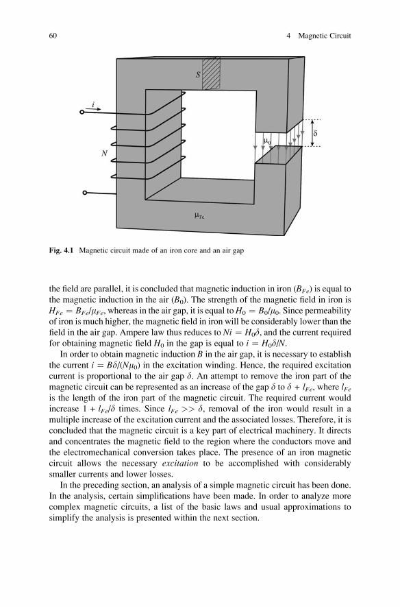
the field are parallel, it is concluded that magnetic induction in iron (BFe) is equal to
the magnetic induction in the air (B0). The strength of the magnetic field in iron is
HFe ¼ BFe/mFe, whereas in the air gap, it is equal toH0 ¼ B0/m0. Since permeability
of iron is much higher, the magnetic field in iron will be considerably lower than the
field in the air gap. Ampere law thus reduces to Ni ¼ H0d, and the current requiredfor obtaining magnetic field H0 in the gap is equal to i ¼ H0d/N.
In order to obtain magnetic induction B in the air gap, it is necessary to establish
the current i ¼ Bd/(Nm0) in the excitation winding. Hence, the required excitation
current is proportional to the air gap d. An attempt to remove the iron part of the
magnetic circuit can be represented as an increase of the gap d to d + lFe, where lFeis the length of the iron part of the magnetic circuit. The required current would
increase 1 + lFe/d times. Since lFe >> d, removal of the iron would result in a
multiple increase of the excitation current and the associated losses. Therefore, it is
concluded that the magnetic circuit is a key part of electrical machinery. It directs
and concentrates the magnetic field to the region where the conductors move and
the electromechanical conversion takes place. The presence of an iron magnetic
circuit allows the necessary excitation to be accomplished with considerably
smaller currents and lower losses.
In the preceding section, an analysis of a simple magnetic circuit has been done.
In the analysis, certain simplifications have been made. In order to analyze more
complex magnetic circuits, a list of the basic laws and usual approximations to
simplify the analysis is presented within the next section.
Fig. 4.1 Magnetic circuit made of an iron core and an air gap
60 4 Magnetic Circuit
4.1 Analysis of Magnetic Circuits
Magnetic circuit is a domain where magnetic field is created by one or several
current circuits or permanent magnets. The laws applicable for analysis of magnetic
circuits are:
• The flux conservation law
• Generalized form of Ampere law
• Constitutive relation B(H) which describes a magnetic material
4.1.1 Flux Conservation Law
þS
~B � d~S ¼ 0: (4.1)
Taking into account ferromagnetic properties of magnetic materials used in making
magnetic circuits, a series of simplifications can be introduced in order to facilitate
their analysis. One of the assumptions is that there is no leakage of magnetic lines
outside magnetic circuit. Neglecting the leakage, it can be shown that the flux
remains constant along the magnetic circuit. In other words, the magnetic flux in
each cross-section of the magnetic circuit is the same. The flux in each cross-section
is also called the core flux or the flux per turn, meaning the flux in a single turn of
the winding encircling the magnetic circuit. The algebraic value of the flux in the
cross-section is defined in accordance with the normal to the cross-section surface,
and it is denoted by F. In most cases, magnetic circuit is encircled by a winding
made of N series-connected turns having the orientation. Assuming that there is no
flux leakage from the magnetic circuit, the flux in each turn is equal toF. Therefore,the flux of the winding isC ¼ NF, with the same reference direction as for the flux
in one turn.
The windings are connected in electrical circuits. The voltage across a winding
is equal to u ¼ Ri + dC/dt, where R is resistance of the series-connected turns, i iswinding current, while dC/dt is back electromotive force. It is of uttermost impor-
tance to match the reference direction of the electrical circuit (current) with the
orientation of the magnetic circuit (flux). As a rule, the reference normal for the flux
is determined from the reference direction of the current by the right-hand rule.
By applying the flux conservation law, it can be shown that the flux in one contour
(turn) is equal to the flux through any other surface leaning on the same contour. This
equality will be used to simplify calculation of the flux in the windings of cylindrical
machines.
Commonly used assumption is that the magnetic field is homogeneous over the
cross-section of a magnetic circuit and that the length of any magnetic field line is
equal to the length of the average representative line of the magnetic circuit.
4.1 Analysis of Magnetic Circuits 61
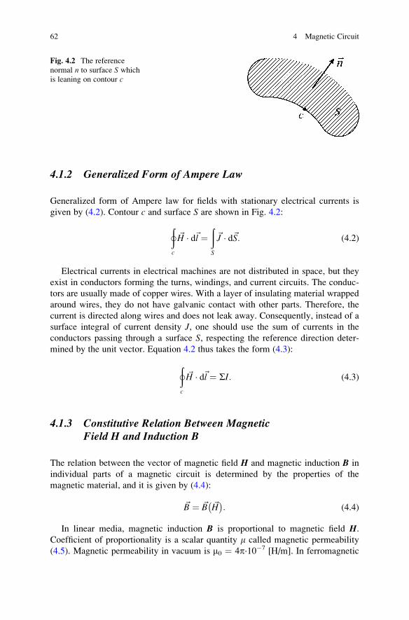
4.1.2 Generalized Form of Ampere Law
Generalized form of Ampere law for fields with stationary electrical currents is
given by (4.2). Contour c and surface S are shown in Fig. 4.2:
þc
~H � d~l ¼ðS
~J � d~S: (4.2)
Electrical currents in electrical machines are not distributed in space, but they
exist in conductors forming the turns, windings, and current circuits. The conduc-
tors are usually made of copper wires. With a layer of insulating material wrapped
around wires, they do not have galvanic contact with other parts. Therefore, the
current is directed along wires and does not leak away. Consequently, instead of a
surface integral of current density J, one should use the sum of currents in the
conductors passing through a surface S, respecting the reference direction deter-
mined by the unit vector. Equation 4.2 thus takes the form (4.3):
þc
~H � d~l ¼ SI: (4.3)
4.1.3 Constitutive Relation Between MagneticField H and Induction B
The relation between the vector of magnetic field H and magnetic induction B in
individual parts of a magnetic circuit is determined by the properties of the
magnetic material, and it is given by (4.4):
~B ¼ ~B ~H� �
: (4.4)
In linear media, magnetic induction B is proportional to magnetic field H.
Coefficient of proportionality is a scalar quantity m called magnetic permeability
(4.5). Magnetic permeability in vacuum is m0 ¼ 4p·10�7 [H/m]. In ferromagnetic
Fig. 4.2 The reference
normal n to surface S which
is leaning on contour c
62 4 Magnetic Circuit
materials like iron, the characteristic B(H) is not linear. It is usually presented
graphically or by the corresponding analytical approximation called the character-istic of magnetization. For small values of magnetic field, the magnetization
characteristic of iron B(H) is linear and has the slope DB/DH which is several
thousand times higher than the permeability of vacuum m0.
~B ¼ m~H ¼ m0mr~H: (4.5)
4.2 The Flux Vector
Flux through the contour of Fig. 4.2 is a scalar quantity. Flux through surface S,leaning on contour c, is determined by surface integral of the vector of magnetic
induction B. In the analysis of electrical machines, flux through a contour is often
considered as a vector. The flux vector is obtained by associating the course and
direction with scalar F. The spatial orientation is obtained from the unit normal to
surface S. In cases with several contours (turns) forming a winding where all of the
contours share the same orientation, it is possible to define the flux vector of the
winding. This flux has algebraic intensity ofC ¼ NF while its course and direction
are determined by the unit normal to surface S. The winding can be made of series-
connected contours (turns) with different spatial orientation. In such cases, the
vector of the winding flux is obtained as a vector sum of flux vectors in individual
contours.
4.3 Magnetizing Characteristic of Ferromagnetic Materials
Magnetic circuits of electrical machines and transformers are most frequently made
of iron sheets. Iron is ferromagnetic material with magnetization characteristic B(H) shown in Fig. 4.3. The characteristic extends between the two straight lines.
The line with the slope DB/DH ¼ m0 describes magnetization characteristic of
vacuum, while the line with the slope mFe corresponds to the first derivative of
the function B(H) at the origin. The abscissa of the B-H coordinate system is the
external field H, which may be obtained by establishing a current in the excitation
winding, while the ordinate is magnetic induction B existing in the ferromagnetic
material.
The magnetic properties of iron originate from microscopic Ampere currents
within a molecule or a group of molecules. These currents make the origin of the
magnetic field of permanent magnets and other ferromagnetic materials. The said
currents are the cause of forces acting on ferromagnetic parts brought in a magnetic
field. The presence of microscopic currents can be taken into account by treating
4.3 Magnetizing Characteristic of Ferromagnetic Materials 63
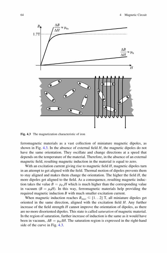
ferromagnetic materials as a vast collection of miniature magnetic dipoles, as
shown in Fig. 4.3. In the absence of external field H, the magnetic dipoles do not
have the same orientation. They oscillate and change directions at a speed that
depends on the temperature of the material. Therefore, in the absence of an external
magnetic field, resulting magnetic induction in the material is equal to zero.
With an excitation current giving rise to magnetic field H, magnetic dipoles turn
in an attempt to get aligned with the field. Thermal motion of dipoles prevents them
to stay aligned and makes them change the orientation. The higher the field H, themore dipoles get aligned to the field. As a consequence, resulting magnetic induc-
tion takes the value B ¼ mFeH which is much higher than the corresponding value
in vacuum (B ¼ m0H). In this way, ferromagnetic materials help providing the
required magnetic induction B with much smaller excitation current.
When magnetic induction reaches Bmax ∈ [1. . .2] T, all miniature dipoles get
oriented in the same direction, aligned with the excitation field H. Any further
increase of the field strength H cannot improve the orientation of dipoles, as there
are no more disoriented dipoles. This state is called saturation of magnetic material.
In the region of saturation, further increase of induction is the same as it would have
been in vacuum, DB ¼ m0DH. The saturation region is expressed in the right-hand
side of the curve in Fig. 4.3.
Fig. 4.3 The magnetization characteristic of iron
64 4 Magnetic Circuit
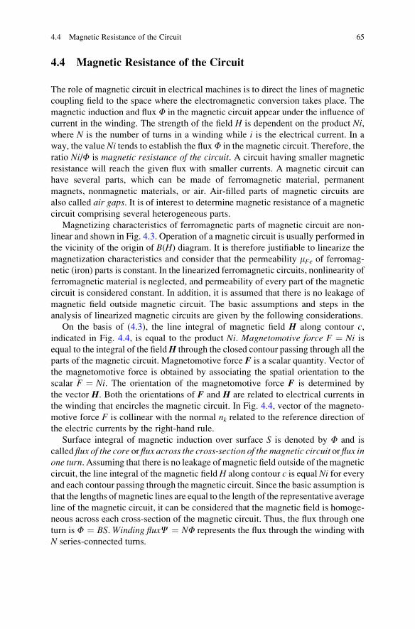
4.4 Magnetic Resistance of the Circuit
The role of magnetic circuit in electrical machines is to direct the lines of magnetic
coupling field to the space where the electromagnetic conversion takes place. The
magnetic induction and flux F in the magnetic circuit appear under the influence of
current in the winding. The strength of the field H is dependent on the product Ni,where N is the number of turns in a winding while i is the electrical current. In a
way, the value Ni tends to establish the fluxF in the magnetic circuit. Therefore, the
ratio Ni/F is magnetic resistance of the circuit. A circuit having smaller magnetic
resistance will reach the given flux with smaller currents. A magnetic circuit can
have several parts, which can be made of ferromagnetic material, permanent
magnets, nonmagnetic materials, or air. Air-filled parts of magnetic circuits are
also called air gaps. It is of interest to determine magnetic resistance of a magnetic
circuit comprising several heterogeneous parts.
Magnetizing characteristics of ferromagnetic parts of magnetic circuit are non-
linear and shown in Fig. 4.3. Operation of a magnetic circuit is usually performed in
the vicinity of the origin of B(H) diagram. It is therefore justifiable to linearize the
magnetization characteristics and consider that the permeability mFe of ferromag-
netic (iron) parts is constant. In the linearized ferromagnetic circuits, nonlinearity of
ferromagnetic material is neglected, and permeability of every part of the magnetic
circuit is considered constant. In addition, it is assumed that there is no leakage of
magnetic field outside magnetic circuit. The basic assumptions and steps in the
analysis of linearized magnetic circuits are given by the following considerations.
On the basis of (4.3), the line integral of magnetic field H along contour c,indicated in Fig. 4.4, is equal to the product Ni. Magnetomotive force F ¼ Ni isequal to the integral of the fieldH through the closed contour passing through all the
parts of the magnetic circuit. Magnetomotive force F is a scalar quantity. Vector of
the magnetomotive force is obtained by associating the spatial orientation to the
scalar F ¼ Ni. The orientation of the magnetomotive force F is determined by
the vector H. Both the orientations of F and H are related to electrical currents in
the winding that encircles the magnetic circuit. In Fig. 4.4, vector of the magneto-
motive force F is collinear with the normal nk related to the reference direction of
the electric currents by the right-hand rule.
Surface integral of magnetic induction over surface S is denoted by F and is
called flux of the core or flux across the cross-section of the magnetic circuit or flux inone turn. Assuming that there is no leakage of magnetic field outside of the magnetic
circuit, the line integral of the magnetic field H along contour c is equal Ni for everyand each contour passing through the magnetic circuit. Since the basic assumption is
that the lengths ofmagnetic lines are equal to the length of the representative average
line of the magnetic circuit, it can be considered that the magnetic field is homoge-
neous across each cross-section of the magnetic circuit. Thus, the flux through one
turn is F ¼ BS.Winding fluxC ¼ NF represents the flux through the winding with
N series-connected turns.
4.4 Magnetic Resistance of the Circuit 65
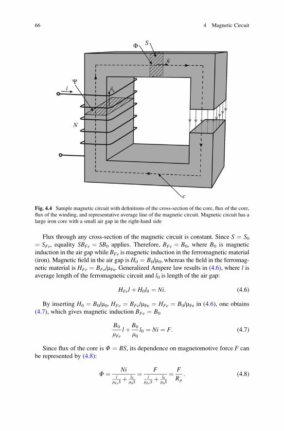
Flux through any cross-section of the magnetic circuit is constant. Since S ¼ S0¼ SFe, equality SBFe ¼ SB0 applies. Therefore, BFe ¼ B0, where B0 is magnetic
induction in the air gap while BFe is magnetic induction in the ferromagnetic material
(iron). Magnetic field in the air gap is H0 ¼ B0/m0, whereas the field in the ferromag-
netic material is HFe ¼ BFe/mFe. Generalized Ampere law results in (4.6), where l isaverage length of the ferromagnetic circuit and l0 is length of the air gap:
HFelþ H0l0 ¼ Ni: (4.6)
By inserting H0 ¼ B0/m0, HFe ¼ BFe/mFe ¼ HFe ¼ B0/mFe in (4.6), one obtains
(4.7), which gives magnetic induction BFe ¼ B0
B0
mFelþ B0
m0l0 ¼ Ni ¼ F: (4.7)
Since flux of the core is F ¼ BS, its dependence on magnetomotive force F can
be represented by (4.8):
F ¼ Nil
mFeSþ l0
m0S
¼ Fl
mFeSþ l0
m0S
¼ F
Rm: (4.8)
Fig. 4.4 Sample magnetic circuit with definitions of the cross-section of the core, flux of the core,
flux of the winding, and representative average line of the magnetic circuit. Magnetic circuit has a
large iron core with a small air gap in the right-hand side
66 4 Magnetic Circuit
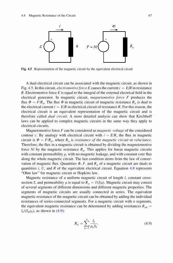
A dual electrical circuit can be associated with the magnetic circuit, as shown in
Fig. 4.5. In this circuit, electromotive force E causes the current i ¼ E/R in resistance
R. Electromotive force E is equal to the integral of the external electrical field in the
electrical generator. In magnetic circuit, magnetomotive force F produces the
flux F ¼ F/Rm. The flux F in magnetic circuit of magnetic resistance Rm is dual to
the electrical current i ¼ E/R in electrical circuit of resistance R. For this reason, theelectrical circuit is an equivalent representation of the magnetic circuit and is
therefore called dual circuit. A more detailed analysis can show that Kirchhoff
laws can be applied to complex magnetic circuits in the same way they apply to
electrical circuits.
Magnetomotive force F can be considered as magnetic voltage of the consideredcontour c. By analogy with electrical circuit with i ¼ E/R, the flux in magnetic
circuit is F ¼ F/Rm, where Rm is resistance of the magnetic circuit or reluctance.Therefore, the flux in a magnetic circuit is obtained by dividing the magnetomotive
force Ni by the magnetic resistance Rm. This applies for linear magnetic circuits
with constant permeability m, with no magnetic leakage, and with constant core flux
along the whole magnetic circuit. The last condition stems from the law of conser-
vation of magnetic flux. Quantities F, F, and Rm of a magnetic circuit are duals to
quantities i, U, and R of the equivalent electrical circuit. Equation 4.8 represents
“Ohm law” for magnetic circuit or Hopkins law.
Magnetic resistance of a uniform magnetic circuit of length l, constant cross-section S, and permeability m is equal to Rm ¼ l/(Sm). Magnetic circuit may consist
of several segments of different dimensions and different magnetic properties. The
segments of magnetic circuits are usually connected in series. The equivalent
magnetic resistance of the magnetic circuit can be obtained by adding the individual
resistances of series-connected segments. For a magnetic circuit with n segments,
the equivalent magnetic resistance can be determined by adding resistances Rmk ¼lk/(Skmk), as shown in (4.9):
Rm ¼Xnk¼1
lkmkSk
: (4.9)
Fig. 4.5 Representation of the magnetic circuit by the equivalent electrical circuit
4.4 Magnetic Resistance of the Circuit 67
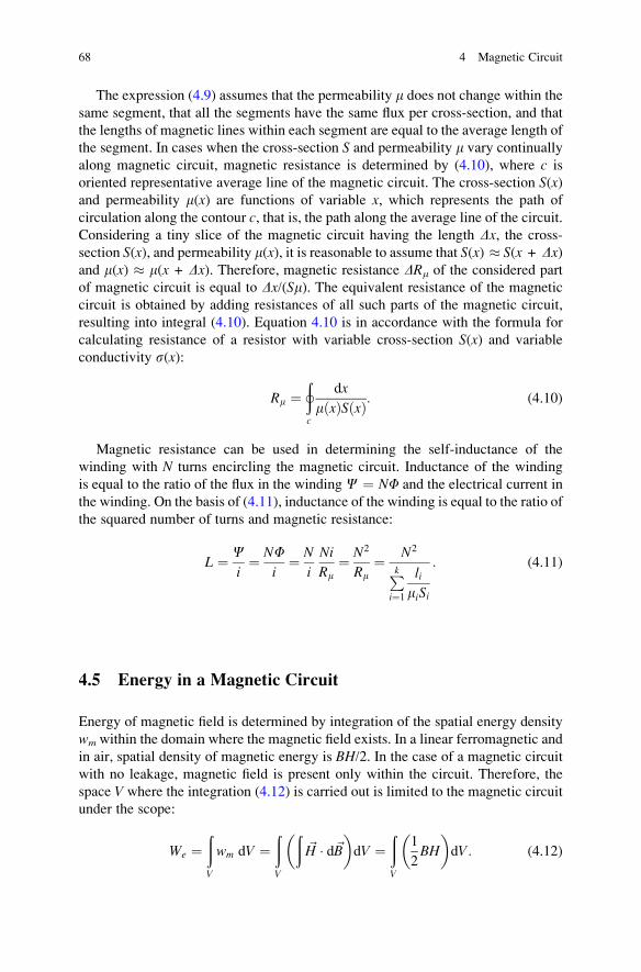
The expression (4.9) assumes that the permeability m does not change within the
same segment, that all the segments have the same flux per cross-section, and that
the lengths of magnetic lines within each segment are equal to the average length of
the segment. In cases when the cross-section S and permeability m vary continually
along magnetic circuit, magnetic resistance is determined by (4.10), where c is
oriented representative average line of the magnetic circuit. The cross-section S(x)and permeability m(x) are functions of variable x, which represents the path of
circulation along the contour c, that is, the path along the average line of the circuit.Considering a tiny slice of the magnetic circuit having the length Dx, the cross-
section S(x), and permeability m(x), it is reasonable to assume that S(x) � S(x + Dx)and m(x) � m(x + Dx). Therefore, magnetic resistance DRm of the considered part
of magnetic circuit is equal to Dx/(Sm). The equivalent resistance of the magnetic
circuit is obtained by adding resistances of all such parts of the magnetic circuit,
resulting into integral (4.10). Equation 4.10 is in accordance with the formula for
calculating resistance of a resistor with variable cross-section S(x) and variable
conductivity s(x):
Rm ¼þc
dx
mðxÞSðxÞ: (4.10)
Magnetic resistance can be used in determining the self-inductance of the
winding with N turns encircling the magnetic circuit. Inductance of the winding
is equal to the ratio of the flux in the winding C ¼ NF and the electrical current in
the winding. On the basis of (4.11), inductance of the winding is equal to the ratio of
the squared number of turns and magnetic resistance:
L ¼ Ci¼ NF
i¼ N
i
Ni
Rm¼ N2
Rm¼ N2
Pki¼1
limiSi
: (4.11)
4.5 Energy in a Magnetic Circuit
Energy of magnetic field is determined by integration of the spatial energy density
wm within the domain where the magnetic field exists. In a linear ferromagnetic and
in air, spatial density of magnetic energy is BH/2. In the case of a magnetic circuit
with no leakage, magnetic field is present only within the circuit. Therefore, the
space V where the integration (4.12) is carried out is limited to the magnetic circuit
under the scope:
We ¼ðV
wm dV ¼ðV
ð~H � d~B
� �dV ¼
ðV
1
2BH
� �dV: (4.12)
68 4 Magnetic Circuit
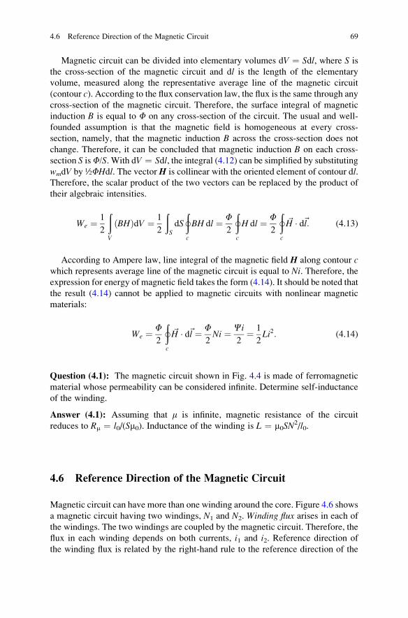
Magnetic circuit can be divided into elementary volumes dV ¼ Sdl, where S is
the cross-section of the magnetic circuit and dl is the length of the elementary
volume, measured along the representative average line of the magnetic circuit
(contour c). According to the flux conservation law, the flux is the same through any
cross-section of the magnetic circuit. Therefore, the surface integral of magnetic
induction B is equal to F on any cross-section of the circuit. The usual and well-
founded assumption is that the magnetic field is homogeneous at every cross-
section, namely, that the magnetic induction B across the cross-section does not
change. Therefore, it can be concluded that magnetic induction B on each cross-
section S isF/S. With dV ¼ Sdl, the integral (4.12) can be simplified by substituting
wmdV by ½FHdl. The vector H is collinear with the oriented element of contour dl.Therefore, the scalar product of the two vectors can be replaced by the product of
their algebraic intensities.
We ¼ 1
2
ðV
BHð ÞdV ¼ 1
2
ðS
dS
þc
BH dl ¼ F2
þc
H dl ¼ F2
þc
~H � d~l: (4.13)
According to Ampere law, line integral of the magnetic field H along contour cwhich represents average line of the magnetic circuit is equal to Ni. Therefore, theexpression for energy of magnetic field takes the form (4.14). It should be noted that
the result (4.14) cannot be applied to magnetic circuits with nonlinear magnetic
materials:
We ¼ F2
þc
~H � d~l ¼ F2Ni ¼ Ci
2¼ 1
2Li2: (4.14)
Question (4.1): The magnetic circuit shown in Fig. 4.4 is made of ferromagnetic
material whose permeability can be considered infinite. Determine self-inductance
of the winding.
Answer (4.1): Assuming that m is infinite, magnetic resistance of the circuit
reduces to Rm ¼ l0/(Sm0). Inductance of the winding is L ¼ m0SN2/l0.
4.6 Reference Direction of the Magnetic Circuit
Magnetic circuit can have more than one winding around the core. Figure 4.6 shows
a magnetic circuit having two windings, N1 and N2. Winding flux arises in each of
the windings. The two windings are coupled by the magnetic circuit. Therefore, the
flux in each winding depends on both currents, i1 and i2. Reference direction of
the winding flux is related by the right-hand rule to the reference direction of the
4.6 Reference Direction of the Magnetic Circuit 69
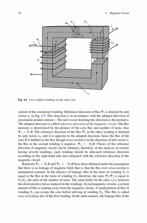
current of the considered winding. Reference direction of fluxC1 is denoted by unit
vector n1 in Fig. 4.5. This direction is in accordance with the adopted direction of
circulation around contour c. The unit vector denoting this direction is the normal n.The adopted direction is called reference direction of the magnetic circuit. The fluxintensity is determined by the product of the core flux and number of turns, thus
C1 ¼ N1F. The reference direction of the flux C2 in the other winding is denoted
by unit vector n2, and it is opposite to the adopted direction. Since the flux of the
core F is defined as the flux though cross-section S in the direction of unit vector n,the flux in the second winding is negative, C2 ¼ �N2F. Choice of the reference
direction of magnetic circuit can be arbitrary; therefore, in the analysis of circuits
having several windings, each winding should be allocated reference direction
according to the right-hand rule and compared with the reference direction of the
magnetic circuit.
RelationsC1 ¼ N1F andC2 ¼ �N2F have been obtained under the assumption
that there is no leakage of magnetic field, that is, that the flux over cross-section is
maintained constant. In the absence of leakage, flux in the turns of winding N1 is
equal to the flux in the turns of winding N2; therefore, the ratio C1/C2 is equal to
N1/N2, the ratio of the number of turns. The same holds for the ratio e1/e2 betweenthe electromotive forces induced in the windings. In real magnetic circuits, a certain
amount of flux is leaking away from the magnetic circuit. A small portion of flux in
winding N1 can escape the core before arriving at winding N2. This flux is called
stray or leakage flux of the first winding. In the same manner, the leakage flux of the
Fig. 4.6 Two coupled windings on the same core
70 4 Magnetic Circuit
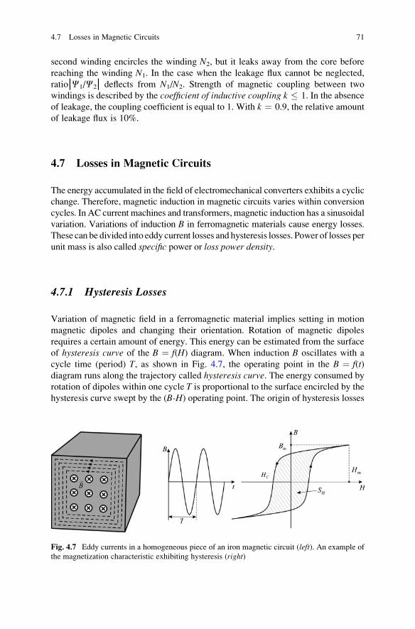
second winding encircles the winding N2, but it leaks away from the core before
reaching the winding N1. In the case when the leakage flux cannot be neglected,
ratio│C1/C2│ deflects from N1/N2. Strength of magnetic coupling between two
windings is described by the coefficient of inductive coupling k � 1. In the absence
of leakage, the coupling coefficient is equal to 1. With k ¼ 0.9, the relative amount
of leakage flux is 10%.
4.7 Losses in Magnetic Circuits
The energy accumulated in the field of electromechanical converters exhibits a cyclic
change. Therefore, magnetic induction in magnetic circuits varies within conversion
cycles. In AC current machines and transformers, magnetic induction has a sinusoidal
variation. Variations of induction B in ferromagnetic materials cause energy losses.
These can be divided into eddy current losses and hysteresis losses. Power of losses per
unit mass is also called specific power or loss power density.
4.7.1 Hysteresis Losses
Variation of magnetic field in a ferromagnetic material implies setting in motion
magnetic dipoles and changing their orientation. Rotation of magnetic dipoles
requires a certain amount of energy. This energy can be estimated from the surface
of hysteresis curve of the B ¼ f(H) diagram. When induction B oscillates with a
cycle time (period) T, as shown in Fig. 4.7, the operating point in the B ¼ f(t)diagram runs along the trajectory called hysteresis curve. The energy consumed by
rotation of dipoles within one cycle T is proportional to the surface encircled by the
hysteresis curve swept by the (B-H) operating point. The origin of hysteresis losses
Fig. 4.7 Eddy currents in a homogeneous piece of an iron magnetic circuit (left). An example of
the magnetization characteristic exhibiting hysteresis (right)
4.7 Losses in Magnetic Circuits 71
is friction between neighboring magnetic dipoles in the course of their cyclic
rotation. This internal friction causes consumption of energy which is converted
into heat.
Specific power losses due to hysteresis pH are proportional to operating
frequency and to surface encircled by the hysteresis curve in the B-H plane. The
energy lost in each operating cycle due to hysteresis in ferromagnetic material of
volume V is
WH ¼ V
þH dB ¼ V � SH; (4.15)
where SH is surface encircled by hysteresis curve. With the operating frequency f,power loss due to hysteresis is
PH ¼ f V � SH: (4.16)
The specific power losses, that is, losses per unit volume, are
pH1 ¼ PH
V¼ f SH: (4.17)
Surface of the hysteresis curve SH depends on the shape of the curve and peak
values of the magnetic field Hm and induction Bm. The surface is proportional to the
product BmHm. The peak values Hm and Bm are in mutual proportion. Therefore,
the surface SH is also proportional to Bm2. Therefore, the losses per unit volume can
be expressed as
pH1 ¼ sH1 � f � B2m: (4.18)
By introducing coefficient sH which is equal to the ratio of the coefficient sH1and specific mass of ferromagnetic material, specific losses due to hysteresis per
unit mass are
pH ¼ sH � f � B2m: (4.19)
4.7.2 Losses Due to Eddy Currents
Ferromagnetic materials are usually conductive. In parts of magnetic circuit that
are made of conductive ferromagnetic, it is possible to envisage toroidal tubes
of conductive material and to consider each of them a closed contour capable of
carrying electrical currents. Variation of magnetic induction B changes the flux in
such contours. As a consequence, electromotive forces are induced in such contours,
72 4 Magnetic Circuit
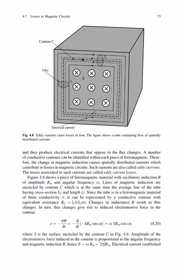
and they produce electrical currents that oppose to the flux changes. A number
of conductive contours can be identified within each piece of ferromagnetic. There-
fore, the change in magnetic induction causes spatially distributed currents which
contribute to losses in magnetic circuits. Such currents are also called eddy currents.The losses associated to such currents are called eddy current losses.
Figure 4.8 shows a piece of ferromagnetic material with oscillatory induction Bof amplitude Bm and angular frequency o. Lines of magnetic induction are
encircled by contour C which is at the same time the average line of the tube
having cross-section SC and length lC. Since the tube is in a ferromagnetic material
of finite conductivity s, it can be represented by a conductive contour with
equivalent resistance RC ¼ lC/(SCs). Changes in inductance B result in flux
changes. In turn, flux changes give rise to induced electromotive force in the
contour
e ¼ � dFdt
¼ � d
dt�SBm sinotð Þ ¼ o SBm cosot; (4.20)
where S is the surface encircled by the contour C in Fig. 4.8. Amplitude of the
electromotive force induced in the contour is proportional to the angular frequency
and magnetic induction B, hence E ~ o Bm ~ 2pfBm. Electrical current established
Fig. 4.8 Eddy currents cause losses in iron. The figure shows a tube containing flow of spatially
distributed currents
4.7 Losses in Magnetic Circuits 73
in the conductive contour is proportional to the electromotive force and inversely
proportional to contour resistance,1 I ~ E/RC ~ 2pfBm/RC. Power losses in the
contour are proportional to resistance RC and square current IC, as given in (4.21):
PC � RCI2C � RC
oBm
RC
� �2� o2B2
m
RC: (4.21)
Therefore, total losses in magnetic circuit due to eddy currents are proportional
to the squared angular frequency and squared magnetic induction. Specific losses
due to eddy currents are
pV ¼ sV � f 2 � Bm2; (4.22)
where sV is coefficient of proportionality, dependent on the specific conductivity
and specific mass of the material.
Question (4.2): The cross-section of magnetic circuit is shown in Fig. 4.8.
Dimensions of these cross-sections are L � L ¼ S. Magnetic induction B is equal
in all points of this cross-section and perpendicular to the surface S. Make an
approximate comparison of eddy current losses at the point which is displaced
from the center by L/2 and at the point which is displaced from the center by L/4.
Answer (4.2): Eddy current can be estimated by considering two contours, the
larger one of radius L/2 and the smaller one with radius L/4. Specific eddy current
losses, that is, the losses per unit volume, depend on the square of the induced
electrical field Ei, pV ~ sEi2. Induced electrical field can be estimated by dividing
the induced electromotive force E of the contour by the length of the contour. The
contour of radius L/2 has four times larger surface and, therefore, four times larger
flux and electromotive force E. Its length is two times larger than the length of the
small contour. Therefore, induced electrical field Ei along the larger contour has
twice the strength of the induced electrical field along the small contour. Finally, the
eddy current losses at the point further away from the center are four times larger.
4.7.3 Total Losses in Magnetic Circuit
The sum of specific losses due to hysteresis and due to eddy currents is given by
(4.23). Specific losses pFe are expressed in W/kg units. With uniform flux density B,the loss distribution in magnetic circuit is uniform as well. In this case, total
magnetic field losses in a magnetic circuit of mass m are PFe ¼ pFem.
pFe ¼ pH þ pV ¼ sH � f � Bm2 þ sV � f 2 � Bm
2: (4.23)
1 Considered contour has resistance RC and self-inductance LC. It has an induced electromotive
force E of angular frequency o. Electrical current in the contour should be calculated by dividing
the electromotive force by the contour impedance ZC ¼ RC + joLC. At lower frequencies whereRC >> oLC, reactance oLC of the contour can be neglected.
74 4 Magnetic Circuit
In magnetic circuits with variable cross-section as well as in cases where the
circuit comprises parts made of different materials and different properties, specific
losses pFe are not the same in all parts of the circuit. Thus, total losses PFe are
determined by integrating specific losses over the volume of the magnetic circuit.
4.7.4 The Methods of Reduction of Iron Losses
Power losses in magnetic circuits of electromechanical converters reduce their
efficiency. In addition, the losses are eventually turned to heat, and they increase
temperature of the magnetic circuit. Overheating can result in damage to the
magnetic circuit or to other nearby parts of the machine. Therefore, it is necessary
to transfer this heat to the environment. In other words, it is necessary to provide the
means for proper cooling. Loss reduction simplifies the cooling system, increases
conversion efficiency, and reduces the amount of heat passed to the environment.
In iron sheets and other ferromagnetic materials used for making magnetic
circuits of electrical machines and transformers, iron losses due to eddy currents
prevail over iron losses due to hysteresis. Eddy current losses are larger than
hysteresis losses by an order of magnitude. The losses can be reduced by taking
additional measures in designing and manufacturing magnetic circuits, thus
increasing the efficiency of electrical machines and preventing their overheating.
By adding silicon and other materials of low specific conductivity into iron used
for making magnetic circuits, specific conductivity of such an alloy is reduced. The
increase of resistance RC of the eddy current contours reduces the amplitude of such
currents (4.21) and reduces eddy current losses.
Another approach to reducing eddy current losses is lamination, the process ofassembling magnetic circuits out of sheets of ferromagnetic material. The sheets
are oriented along direction of the magnetic field, in the way shown in Fig. 4.9.
A laminar magnetic circuit is not made of solid iron, but of iron sheets which are
electrically isolated from one another.
Since the sheets are parallel with magnetic field, contours of induced eddy
currents are perpendicular to the field. Electrical insulation between neighboring
layers prevents eddy currents; thus, they can be formed only within individual
layers. It can be shown that this contributes to a considerable reduction of eddy
current losses.
Iron sheets used for designing magnetic circuits of line-frequency transformers
(50 or 60 Hz) and conventional electrical machines are 0.2–0.5 mm thick. Insula-
tion between the sheets is made by inserting thin layers of insulating material
(paper, lacquer) or by short-time exposure of iron sheets to an acid which forms a
thin layer of nonconductive iron compound (salt).
In contemporary electrical machines used in electrical vehicles, hybrid cars, and
alternative power sources, the operating frequency may be in excess of 1 kHz.
Magnetic circuits of such machines are made of very thin iron sheets (0.05–0.1 mm)
or of amorphous strips based on alloys of iron, manganese, and other metals, as well
4.7 Losses in Magnetic Circuits 75
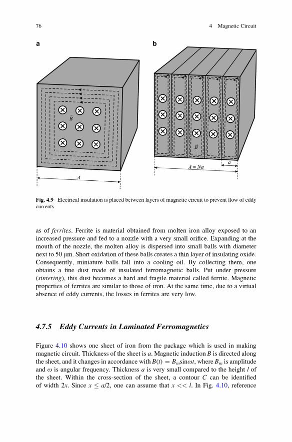
as of ferrites. Ferrite is material obtained from molten iron alloy exposed to an
increased pressure and fed to a nozzle with a very small orifice. Expanding at the
mouth of the nozzle, the molten alloy is dispersed into small balls with diameter
next to 50 mm. Short oxidation of these balls creates a thin layer of insulating oxide.
Consequently, miniature balls fall into a cooling oil. By collecting them, one
obtains a fine dust made of insulated ferromagnetic balls. Put under pressure
(sintering), this dust becomes a hard and fragile material called ferrite. Magnetic
properties of ferrites are similar to those of iron. At the same time, due to a virtual
absence of eddy currents, the losses in ferrites are very low.
4.7.5 Eddy Currents in Laminated Ferromagnetics
Figure 4.10 shows one sheet of iron from the package which is used in making
magnetic circuit. Thickness of the sheet is a. Magnetic induction B is directed along
the sheet, and it changes in accordance with B(t) ¼ Bmsinot, where Bm is amplitude
and o is angular frequency. Thickness a is very small compared to the height l ofthe sheet. Within the cross-section of the sheet, a contour C can be identified
of width 2x. Since x � a/2, one can assume that x << l. In Fig. 4.10, reference
Fig. 4.9 Electrical insulation is placed between layers of magnetic circuit to prevent flow of eddy
currents
76 4 Magnetic Circuit
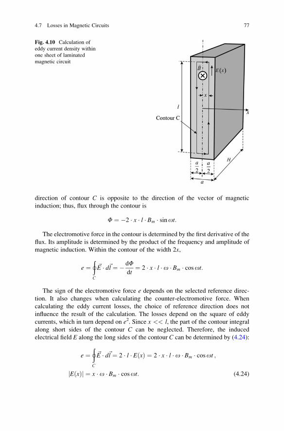
direction of contour C is opposite to the direction of the vector of magnetic
induction; thus, flux through the contour is
F ¼ �2 � x � l � Bm � sinot:
The electromotive force in the contour is determined by the first derivative of the
flux. Its amplitude is determined by the product of the frequency and amplitude of
magnetic induction. Within the contour of the width 2x,
e ¼þC
~E � d~l ¼ � dFdt
¼ 2 � x � l � o � Bm � cosot:
The sign of the electromotive force e depends on the selected reference direc-
tion. It also changes when calculating the counter-electromotive force. When
calculating the eddy current losses, the choice of reference direction does not
influence the result of the calculation. The losses depend on the square of eddy
currents, which in turn depend on e2. Since x << l, the part of the contour integralalong short sides of the contour C can be neglected. Therefore, the induced
electrical field E along the long sides of the contour C can be determined by (4.24):
e ¼þC
~E � d~l ¼ 2 � l � EðxÞ ¼ 2 � x � l � o � Bm � cosot ;
EðxÞj j ¼ x � o � Bm � cosot: (4.24)
Fig. 4.10 Calculation of
eddy current density within
one sheet of laminated
magnetic circuit
4.7 Losses in Magnetic Circuits 77
In ferromagnetic material of specific conductivity s exposed to induced electri-
cal field E, the density of spatial currents is J ¼ sE. In the considered sheet of iron,current density is
JðxÞ ¼ sEðxÞ ¼ s � x � o � Bm � cosot:
Spatial currents in material of finite conductivity give rise to power losses also
called Joule losses. Specific power of these losses is equal to the product of the
current density and algebraic intensity of electrical field,
pFeðxÞ ¼ DPDV
¼ sE2ðxÞ ¼ J2ðxÞs
¼ s � x � o � Bm � cosotð Þ2:
Total losses P1Fe in a single sheet of ferromagnetic material of dimensions
a � l � H are obtained by spatial integration and are determined by (4.25):
P1Fe ¼ðV
pFeðxÞdV ¼ 2 �ða20
H � l � s � x � o � Bm � cosotð Þ2dx
¼ a3
12H � l � s � Bm
2 � o2 � cosotð Þ2 ¼ k � a3 � Bm2 � o2: (4.25)
Coefficient k is dependent on the dimensions H and l, specific conductivity s,and factor cos2ot, whose average value is 0.5. Result (4.25) can be used in the
analysis of the reduction of losses due to splitting magnetic core to layers (sheets) of
thickness a.Figure 4.9a shows a homogenous piece of ferromagnetic material which could
be considered as one layer of thickness a ¼ A. Starting from the assumption that
thickness of the considered part is considerably smaller than the height, it is
possible to apply the result (4.25) and determine losses Phom by (4.26):
Phom ¼ k � Bm2 � o2 � A3: (4.26)
The considered part of magnetic circuit can be made to consist of N mutually
insulated layers (sheets) of thickness a ¼ A/N, as shown in Fig. 4.9b. If the layer ofelectrical insulation between the ferromagnetic sheets is considerably smaller than
a, it can be assumed that the cross-section of laminated magnetic circuit is filled
with iron. Therefore, magnetic resistance of laminated magnetic circuit is equal to
the resistance of magnetic circuit of the same shape, made of homogenous piece of
ferromagnetic material, as shown in Fig. 4.9a. Equation 4.25 gives the eddy current
losses P1Fe in one sheet (layer), whatever the size. It has been applied (4.26) to
homogeneous magnetic circuit in Fig. 4.9a, which is considered as a single sheet
of iron, N times wider than the sheets shown in Fig. 4.9b, where the total number of
78 4 Magnetic Circuit
such sheets is assumed to be N. The losses Plam in laminated magnetic circuit of
width A ¼ aN are determined by expression (4.27):
Plam ¼ N k � Bm2 � o2 � A
N
� �3
¼ k � Bm2 � o2 � A � a2 ¼ Phom
N2: (4.27)
Result (4.27) indicates that losses due to eddy currents in a part of magnetic
circuit of given dimensions decrease N2 times if the ferromagnetic material is split
into N insulated layers (sheets) of equal thickness oriented along the direction of
magnetic field. In cases with variable magnetic field perpendicular to the iron
sheets, the lamination does not reduce the eddy current losses. In addition, lamina-
tion of a magnetic circuit does not reduce the losses due to hysteresis.
In the case of a well-positioned laminar structure of magnetic circuit, losses due
to eddy currents are proportional to the squared laminar thickness a, which leads tothe conclusion that one should be using iron sheets as thin as possible. Conse-
quently, the question arises, why not use the iron sheets thinner than 0.1 � 0.2 mm?
Thinner sheets are more difficult to cut and to assemble. At the same time, a
decrease in thickness would reduce the equivalent cross-section of iron, decrease
the peak flux, and increase the magnetic resistance. Namely, there is an insulating
layer between the sheets, made of paper or nonconductive iron compounds. It is
several tens of micrometers thick, and it exists on both sides of the sheets. Any
further reduction of sheet thickness would reduce the amount of iron in the cross-
section of magnetic circuit below reason.
In magnetic circuits made of solid material where eddy currents are considerable,
magnetic field does not have homogeneous distribution over the cross-section.
An increase in operating frequency leads to significant eddy currents which, in
turn, result in uneven distribution of magnetic induction B across the cross-section
of the core. Namely, eddy currents create magnetic field which opposes to variations
ofmagnetic induction in the core. Such an effect of eddy currents is more emphasized
in the middle of the core, the region which is encircled by all the eddy current
contours (see Fig. 4.9a). This phenomenon results in difference between magnetic
induction in the center of the core and the induction at the peripheral regions.
In magnetic circuits made of iron sheets, these effects are reduced considerably,
and there is no significant difference in the field intensity across the cross-section of
the core.
4.7 Losses in Magnetic Circuits 79
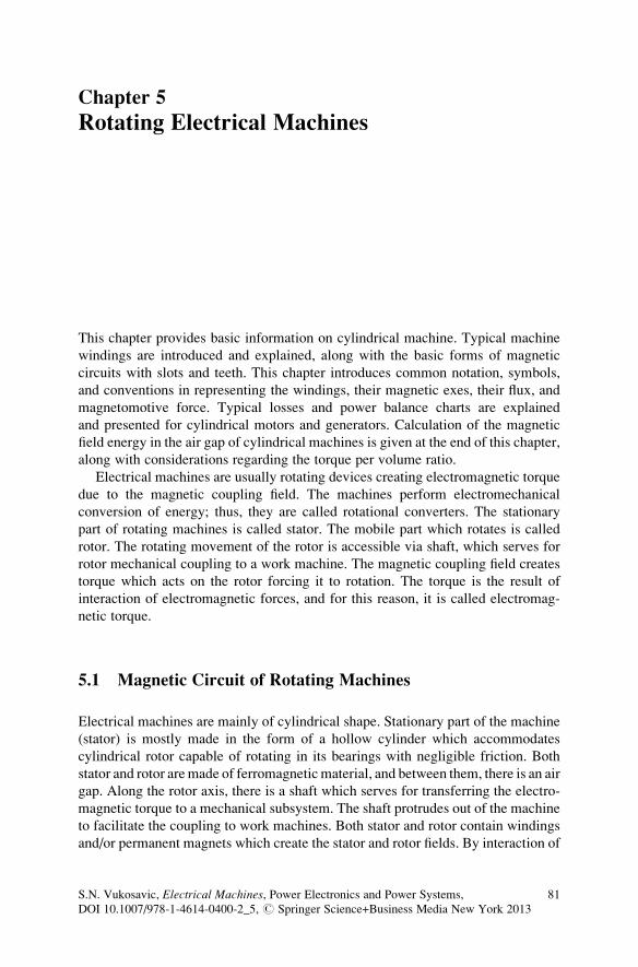
Chapter 5
Rotating Electrical Machines
This chapter provides basic information on cylindrical machine. Typical machine
windings are introduced and explained, along with the basic forms of magnetic
circuits with slots and teeth. This chapter introduces common notation, symbols,
and conventions in representing the windings, their magnetic exes, their flux, and
magnetomotive force. Typical losses and power balance charts are explained
and presented for cylindrical motors and generators. Calculation of the magnetic
field energy in the air gap of cylindrical machines is given at the end of this chapter,
along with considerations regarding the torque per volume ratio.
Electrical machines are usually rotating devices creating electromagnetic torque
due to the magnetic coupling field. The machines perform electromechanical
conversion of energy; thus, they are called rotational converters. The stationary
part of rotating machines is called stator. The mobile part which rotates is called
rotor. The rotating movement of the rotor is accessible via shaft, which serves for
rotor mechanical coupling to a work machine. The magnetic coupling field creates
torque which acts on the rotor forcing it to rotation. The torque is the result of
interaction of electromagnetic forces, and for this reason, it is called electromag-
netic torque.
5.1 Magnetic Circuit of Rotating Machines
Electrical machines are mainly of cylindrical shape. Stationary part of the machine
(stator) is mostly made in the form of a hollow cylinder which accommodates
cylindrical rotor capable of rotating in its bearings with negligible friction. Both
stator and rotor aremade of ferromagneticmaterial, and between them, there is an air
gap. Along the rotor axis, there is a shaft which serves for transferring the electro-
magnetic torque to a mechanical subsystem. The shaft protrudes out of the machine
to facilitate the coupling to work machines. Both stator and rotor contain windings
and/or permanent magnets which create the stator and rotor fields. By interaction of
S.N. Vukosavic, Electrical Machines, Power Electronics and Power Systems,
DOI 10.1007/978-1-4614-0400-2_5, # Springer Science+Business Media New York 2013
81
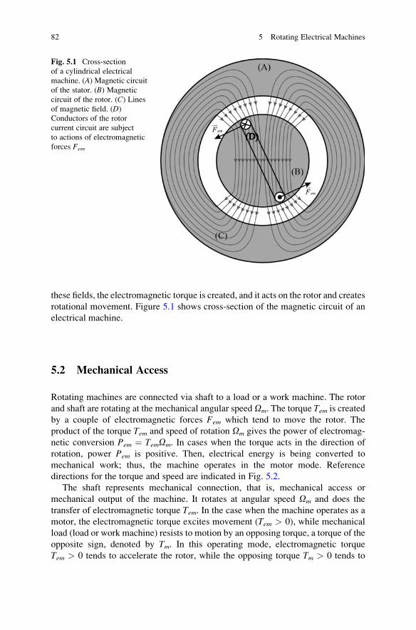
these fields, the electromagnetic torque is created, and it acts on the rotor and creates
rotational movement. Figure 5.1 shows cross-section of the magnetic circuit of an
electrical machine.
5.2 Mechanical Access
Rotating machines are connected via shaft to a load or a work machine. The rotor
and shaft are rotating at the mechanical angular speed Om. The torque Tem is created
by a couple of electromagnetic forces Fem which tend to move the rotor. The
product of the torque Tem and speed of rotation Om gives the power of electromag-
netic conversion Pem ¼ TemOm. In cases when the torque acts in the direction of
rotation, power Pem is positive. Then, electrical energy is being converted to
mechanical work; thus, the machine operates in the motor mode. Reference
directions for the torque and speed are indicated in Fig. 5.2.
The shaft represents mechanical connection, that is, mechanical access or
mechanical output of the machine. It rotates at angular speed Om and does the
transfer of electromagnetic torque Tem. In the case when the machine operates as a
motor, the electromagnetic torque excites movement (Tem > 0), while mechanical
load (load or work machine) resists to motion by an opposing torque, a torque of the
opposite sign, denoted by Tm. In this operating mode, electromagnetic torque
Tem > 0 tends to accelerate the rotor, while the opposing torque Tm > 0 tends to
Fig. 5.1 Cross-section
of a cylindrical electrical
machine. (A) Magnetic circuit
of the stator. (B) Magnetic
circuit of the rotor. (C) Linesof magnetic field. (D)Conductors of the rotor
current circuit are subject
to actions of electromagnetic
forces Fem
82 5 Rotating Electrical Machines
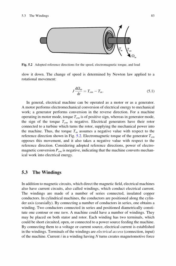
slow it down. The change of speed is determined by Newton law applied to a
rotational movement:
JdOm
dt¼ Tem � Tm: (5.1)
In general, electrical machine can be operated as a motor or as a generator.
A motor performs electromechanical conversion of electrical energy to mechanical
work; a generator performs conversion in the reverse direction. For a machine
operating in motor mode, torque Tem is of positive sign, whereas in generator mode,
the sign of the torque Tem is negative. Electrical generators have their rotor
connected to a turbine which turns the rotor, supplying the mechanical power into
the machine. Thus, the torque Tm assumes a negative value with respect to the
reference direction shown in Fig. 5.2. Electromagnetic torque of the generator Temopposes this movement, and it also takes a negative value with respect to the
reference direction. Considering adopted reference directions, power of electro-
magnetic conversion Pem is negative, indicating that the machine converts mechan-
ical work into electrical energy.
5.3 The Windings
In addition to magnetic circuits, which direct the magnetic field, electrical machines
also have current circuits, also called windings, which conduct electrical current.
The windings are made of a number of series connected, insulated copper
conductors. In cylindrical machines, the conductors are positioned along the cylin-
der axis (coaxially). By connecting a number of conductors in series, one obtains a
winding. Two conductors connected in series and positioned diametrically consti-
tute one contour or one turn. A machine could have a number of windings. They
may be placed on both stator and rotor. Each winding has two terminals, which
could be short circuited, open, or connected to a power source feeding the machine.
By connecting them to a voltage or current source, electrical current is established
in the windings. Terminals of the windings are electrical access (connection, input)of the machine. Current i in a winding having N turns creates magnetomotive force
Fig. 5.2 Adopted reference directions for the speed, electromagnetic torque, and load
5.3 The Windings 83
of F ¼ Ni. By dividing the magnetomotive force with magnetic resistance Rm, one
obtains flux F. Stator windings create stator flux, whereas rotor windings create
rotor flux. There are machines where stator or rotor does not have windings, but
the flux is created by permanent magnets.
The resultant flux of themachine is obtained by joint action of themagnetomotive
forces of the stator and rotor. Lines of the resulting field run through the magnetic
circuit of rotor, air gap, and magnetic circuit of stator. Figure 5.3(A) shows the
lines of magnetic field in the air gap. The figure shows the zone wheremagnetic lines
leave magnetic circuit of the rotor and enter the air gap.1 This zone is called north
Fig. 5.3 Magnetic field in the air gap and windings of an electrical machine. (A) An approximate
appearance of the lines of the resultant magnetic field in the air gap. (B) Magnetic circuits of the
stator and rotor. (C) Coaxially positioned conductors. (D) Air gap. (E) Notation used for the
windings
1 Figure 5.3 shows an approximate shape of the lines of magnetic field in the air gap, which does
not correspond to the air gap field of real machines. Electrical machines have magnetic circuit
containing slots and teeth which are described in the following subsections. The presence of slots
has an influence on the shape of the air gap field, making it relatively more complicated. In the
hypothetical case when the magnetic circuit is of an ideal cylindrical shape and permeability of
the ferromagnetic material is considerably higher than that of the air, the lines of magnetic field are
perpendicular to the surface separating the air gap and the ferromagnetic material. It is of interest
to envisage the surface that separates the air gap from the ferromagnetic material. The boundary
conditions relate tangential components of magnetic field H on either side of this surface with
surface electrical currents JS. With JS ¼ 0, tangential component of magnetic field H in the air is
equal to tangential component of magnetic field in ferromagnetic material. Since BFe < 1.7 T and
HFe ¼ BFe/mFe � 0, tangential component of magnetic field in the air is close to zero. Thus, the
lines of magnetic field in the air gap are perpendicular to the surface separating the air gap and
the ferromagnetic circuit.
84 5 Rotating Electrical Machines
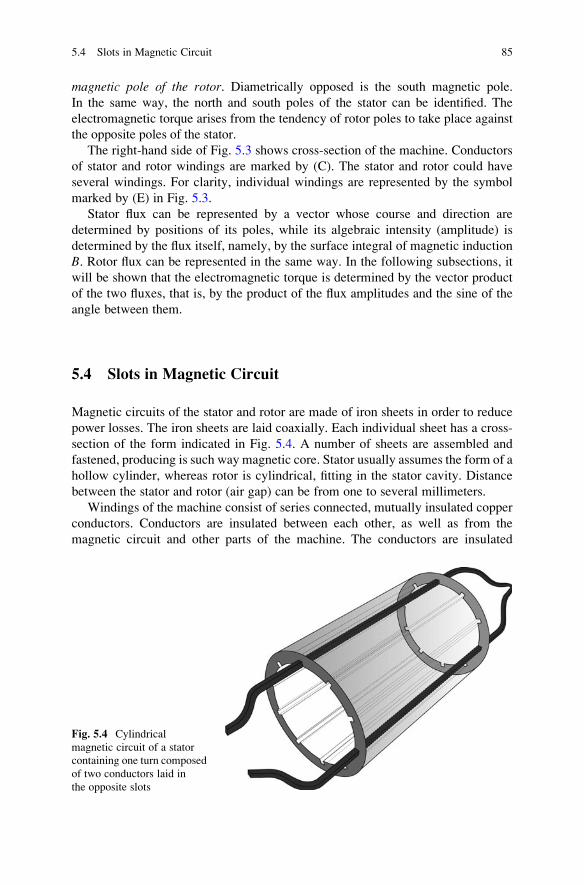
magnetic pole of the rotor. Diametrically opposed is the south magnetic pole.
In the same way, the north and south poles of the stator can be identified. The
electromagnetic torque arises from the tendency of rotor poles to take place against
the opposite poles of the stator.
The right-hand side of Fig. 5.3 shows cross-section of the machine. Conductors
of stator and rotor windings are marked by (C). The stator and rotor could have
several windings. For clarity, individual windings are represented by the symbol
marked by (E) in Fig. 5.3.
Stator flux can be represented by a vector whose course and direction are
determined by positions of its poles, while its algebraic intensity (amplitude) is
determined by the flux itself, namely, by the surface integral of magnetic induction
B. Rotor flux can be represented in the same way. In the following subsections, it
will be shown that the electromagnetic torque is determined by the vector product
of the two fluxes, that is, by the product of the flux amplitudes and the sine of the
angle between them.
5.4 Slots in Magnetic Circuit
Magnetic circuits of the stator and rotor are made of iron sheets in order to reduce
power losses. The iron sheets are laid coaxially. Each individual sheet has a cross-
section of the form indicated in Fig. 5.4. A number of sheets are assembled and
fastened, producing is such way magnetic core. Stator usually assumes the form of a
hollow cylinder, whereas rotor is cylindrical, fitting in the stator cavity. Distance
between the stator and rotor (air gap) can be from one to several millimeters.
Windings of the machine consist of series connected, mutually insulated copper
conductors. Conductors are insulated between each other, as well as from the
magnetic circuit and other parts of the machine. The conductors are insulated
Fig. 5.4 Cylindrical
magnetic circuit of a stator
containing one turn composed
of two conductors laid in
the opposite slots
5.4 Slots in Magnetic Circuit 85
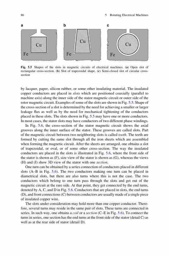
by lacquer, paper, silicon rubber, or some other insulating material. The insulated
copper conductors are placed in slots which are positioned coaxially (parallel to
machine axis) along the inner side of the stator magnetic circuit or outer side of the
rotor magnetic circuit. Examples of some of the slots are shown in Fig. 5.5. Shape of
the cross-section of a slot is determined by the need for achieving a smaller or larger
leakage flux as well as by the need for mechanical tightening of the conductors
placed in these slots. The slots shown in Fig. 5.5 may have one or more conductors.
In most cases, the stator slots may have conductors of two different phase windings.
In Fig. 5.6, the cross-section of the stator magnetic circuit shows the axial
grooves along the inner surface of the stator. These grooves are called slots. Part
of the magnetic circuit between two neighboring slots is called tooth. The teeth are
formed by cutting the same slot through all the iron sheets which are assembled
when forming the magnetic circuit. After the sheets are arranged, one obtains a slot
of trapezoidal, or oval, or of some other cross-section. The way the insulated
conductors are placed in the slots is illustrated in Fig. 5.6, where the front side of
the stator is shown as (F), size view of the stator is shown as (G), whereas the views
(H) and (I) show 3D view of the stator with one section.One turn can be obtained by a series connection of conductors placed in different
slots (A–B in Fig. 5.6). The two conductors making one turn can be placed in
diametrical slots, but there are also turns where this is not the case. The two
conductors which belong to one turn pass through the slots and get out of the
magnetic circuit at the rare side. At that point, they get connected by the end turns,
denoted by A, C, and D in Fig. 5.6. Conductors that are placed in slots, the end turns
(D), and front connections (C) between conductors are usuallymade of a single piece
of insulated copper wire.
The slots under consideration may hold more than one copper conductor. There-
fore, several turns may reside in the same pair of slots. These turns are connected in
series. In such way, one obtains a coil or a section (C–E in Fig. 5.6). To connect the
turns in series, one section has the end turns at the front side of the stator (detail C) as
well as at the rear side of stator (detail D).
Fig. 5.5 Shapes of the slots in magnetic circuits of electrical machines. (a) Open slot of
rectangular cross-section. (b) Slot of trapezoidal shape. (c) Semi-closed slot of circular cross-
section
86 5 Rotating Electrical Machines
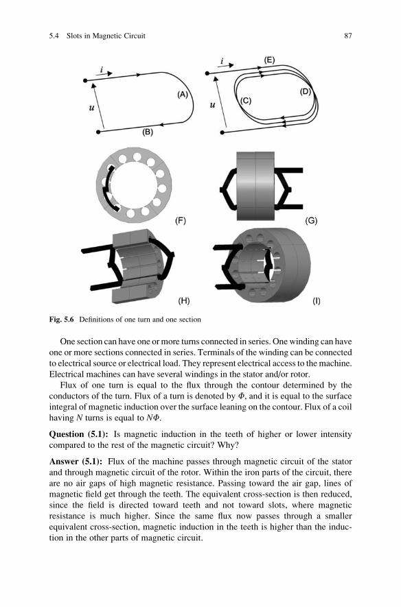
One section can have one or more turns connected in series. Onewinding can have
one or more sections connected in series. Terminals of the winding can be connected
to electrical source or electrical load. They represent electrical access to the machine.
Electrical machines can have several windings in the stator and/or rotor.
Flux of one turn is equal to the flux through the contour determined by the
conductors of the turn. Flux of a turn is denoted by F, and it is equal to the surface
integral of magnetic induction over the surface leaning on the contour. Flux of a coil
having N turns is equal to NF.
Question (5.1): Is magnetic induction in the teeth of higher or lower intensity
compared to the rest of the magnetic circuit? Why?
Answer (5.1): Flux of the machine passes through magnetic circuit of the stator
and through magnetic circuit of the rotor. Within the iron parts of the circuit, there
are no air gaps of high magnetic resistance. Passing toward the air gap, lines of
magnetic field get through the teeth. The equivalent cross-section is then reduced,
since the field is directed toward teeth and not toward slots, where magnetic
resistance is much higher. Since the same flux now passes through a smaller
equivalent cross-section, magnetic induction in the teeth is higher than the induc-
tion in the other parts of magnetic circuit.
Fig. 5.6 Definitions of one turn and one section
5.4 Slots in Magnetic Circuit 87
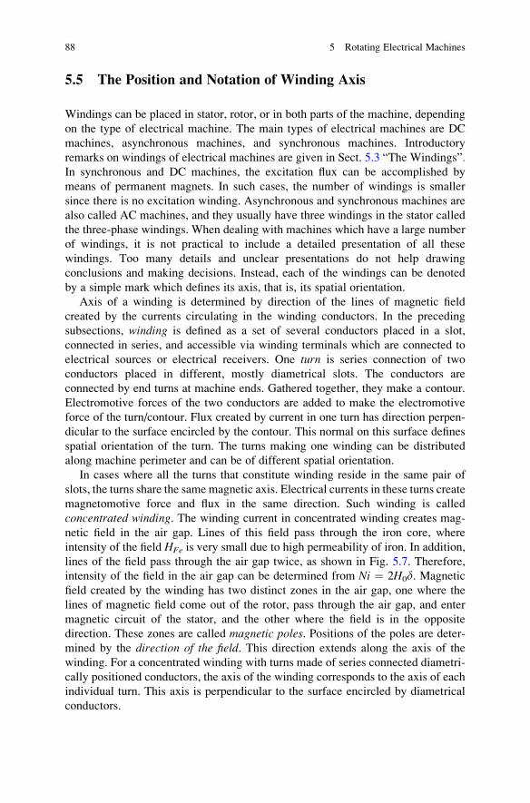
5.5 The Position and Notation of Winding Axis
Windings can be placed in stator, rotor, or in both parts of the machine, depending
on the type of electrical machine. The main types of electrical machines are DC
machines, asynchronous machines, and synchronous machines. Introductory
remarks on windings of electrical machines are given in Sect. 5.3 “The Windings”.In synchronous and DC machines, the excitation flux can be accomplished by
means of permanent magnets. In such cases, the number of windings is smaller
since there is no excitation winding. Asynchronous and synchronous machines are
also called AC machines, and they usually have three windings in the stator called
the three-phase windings. When dealing with machines which have a large number
of windings, it is not practical to include a detailed presentation of all these
windings. Too many details and unclear presentations do not help drawing
conclusions and making decisions. Instead, each of the windings can be denoted
by a simple mark which defines its axis, that is, its spatial orientation.
Axis of a winding is determined by direction of the lines of magnetic field
created by the currents circulating in the winding conductors. In the preceding
subsections, winding is defined as a set of several conductors placed in a slot,
connected in series, and accessible via winding terminals which are connected to
electrical sources or electrical receivers. One turn is series connection of two
conductors placed in different, mostly diametrical slots. The conductors are
connected by end turns at machine ends. Gathered together, they make a contour.
Electromotive forces of the two conductors are added to make the electromotive
force of the turn/contour. Flux created by current in one turn has direction perpen-
dicular to the surface encircled by the contour. This normal on this surface defines
spatial orientation of the turn. The turns making one winding can be distributed
along machine perimeter and can be of different spatial orientation.
In cases where all the turns that constitute winding reside in the same pair of
slots, the turns share the same magnetic axis. Electrical currents in these turns create
magnetomotive force and flux in the same direction. Such winding is called
concentrated winding. The winding current in concentrated winding creates mag-
netic field in the air gap. Lines of this field pass through the iron core, where
intensity of the field HFe is very small due to high permeability of iron. In addition,
lines of the field pass through the air gap twice, as shown in Fig. 5.7. Therefore,
intensity of the field in the air gap can be determined from Ni ¼ 2H0d. Magnetic
field created by the winding has two distinct zones in the air gap, one where the
lines of magnetic field come out of the rotor, pass through the air gap, and enter
magnetic circuit of the stator, and the other where the field is in the opposite
direction. These zones are called magnetic poles. Positions of the poles are deter-
mined by the direction of the field. This direction extends along the axis of the
winding. For a concentrated winding with turns made of series connected diametri-
cally positioned conductors, the axis of the winding corresponds to the axis of each
individual turn. This axis is perpendicular to the surface encircled by diametrical
conductors.
88 5 Rotating Electrical Machines
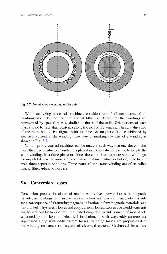
While analyzing electrical machines, consideration of all conductors of all
windings would be too complex and of little use. Therefore, the windings are
represented by special marks, similar to those of the coils. Orientations of each
mark should be such that it extends along the axis of the winding. Namely, direction
of the mark should be aligned with the lines of magnetic field established by
electrical current in the winding. The way of marking the axis of a winding is
shown in Fig. 5.7.
Windings of electrical machines can be made in such way that one slot contains
more than one conductor. Conductors placed in one slot do not have to belong to the
same winding. In a three-phase machine, there are three separate stator windings,
having a total of six terminals. One slot may contain conductors belonging to two or
even three separate windings. Three parts of one stator winding are often called
phases (three-phase windings).
5.6 Conversion Losses
Conversion process in electrical machines involves power losses in magnetic
circuits, in windings, and in mechanical subsystem. Losses in magnetic circuits
are a consequence of alternating magnetic induction in ferromagnetic materials, and
it is divided in hysteresis losses and eddy currents losses. Losses due to eddy currents
can be reduced by lamination. Laminated magnetic circuit is made of iron sheets
separated by thin layers of electrical insulation. In such way, eddy currents are
suppressed along with eddy current losses. Winding losses are proportional to
the winding resistance and square of electrical current. Mechanical losses are
Fig. 5.7 Notation of a winding and its axis
5.6 Conversion Losses 89
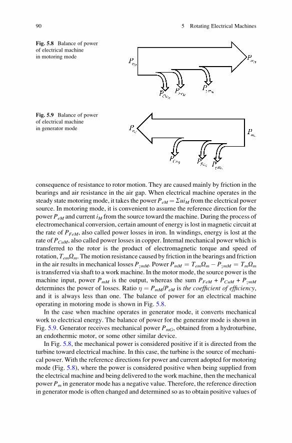
consequence of resistance to rotor motion. They are caused mainly by friction in the
bearings and air resistance in the air gap. When electrical machine operates in the
steady state motoring mode, it takes the power PeM¼SuiM from the electrical power
source. In motoring mode, it is convenient to assume the reference direction for the
power PeM and current iM from the source toward the machine. During the process of
electromechanical conversion, certain amount of energy is lost in magnetic circuit at
the rate of PFeM, also called power losses in iron. In windings, energy is lost at the
rate of PCuM, also called power losses in copper. Internal mechanical power which is
transferred to the rotor is the product of electromagnetic torque and speed of
rotation, TemOm. Themotion resistance caused by friction in the bearings and friction
in the air results in mechanical losses PgmM. Power PmM ¼ TemOm� PgmM ¼ TmOm
is transferred via shaft to a workmachine. In the motor mode, the source power is the
machine input, power PmM is the output, whereas the sum PFeM + PCuM + PgmM
determines the power of losses. Ratio � ¼ PmM/PeM is the coefficient of efficiency,and it is always less than one. The balance of power for an electrical machine
operating in motoring mode is shown in Fig. 5.8.
In the case when machine operates in generator mode, it converts mechanical
work to electrical energy. The balance of power for the generator mode is shown in
Fig. 5.9. Generator receives mechanical power PmG, obtained from a hydroturbine,
an endothermic motor, or some other similar device.
In Fig. 5.8, the mechanical power is considered positive if it is directed from the
turbine toward electrical machine. In this case, the turbine is the source of mechani-
cal power. With the reference directions for power and current adopted for motoring
mode (Fig. 5.8), where the power is considered positive when being supplied from
the electrical machine and being delivered to the work machine, then the mechanical
power Pm in generator mode has a negative value. Therefore, the reference direction
in generator mode is often changed and determined so as to obtain positive values of
Fig. 5.8 Balance of power
of electrical machine
in motoring mode
Fig. 5.9 Balance of power
of electrical machine
in generator mode
90 5 Rotating Electrical Machines
power PmG, received from the turbine, and a positive value of power PeG, supplied
by the generator to electrical circuits and receivers, connected to the stator winding.
The same reference direction is usually taken for the electrical current iG.Power PmG represents input to the generator, and it comes from the turbine or
other source of mechanical power. Within the machine, one part of the input power
is lost on overcoming motion resistances encountered by the rotor. By subtracting
power PgmG from input power PmG, one obtains internal mechanical power which is
converted to electrical power. One part of the obtained electrical power is lost in
windings, where the copper losses are PCuG, and in magnetic circuit, where the iron
losses are PFeG. The remaining power is at disposal to electrical consumers supplied
by the generator. At the ends of stator winding, one obtains currents and voltages
which determine the generated electrical power PeG ¼ SuiG, which can be trans-
ferred to electrical consumers.
The coefficient of efficiency can be increased by designing the machine to have
reduced losses windings (copper losses) and magnetic circuit (iron losses). By
increasing the cross-section of conductors, the resistance of copper conductors is
decreased which leads to reduced copper losses. By increasing the cross-section of
magnetic circuit, the magnetic induction decreases for the same flux. Consequently,
the iron losses are smaller. On the other hand, this approach to reducing the
current density and magnetic induction leads to an increased volume and mass of
themachine. The specific power, determined by the ratio of the power andmass of the
machine, becomes smaller as well. Therefore, for an electrical machine of predefined
power, decreased current and flux densities lead to an increase in quantities of copper
and iron used to make the machine. At the same time, dimensions of the machine are
increased as well.
Design policy of reducing the flux and current densities decreases the overall
energy losses in copper and iron in the course of electrical machine service.
Nevertheless, the overall effects of this design policy may eventually be negative.
Namely, the increase in efficiency is obtained on account of an increased consump-
tion of iron and copper. At this point, along with the energy spent during the
operating lifetime of electrical machines, it is of interest to take into account
the energy spent in their manufacturing. Production of the electrolytic copper,
used to make the windings, requires considerable amounts of energy. The same
way, production of insulated iron sheets for making magnetic circuits requires
energy. Therefore, the energy savings due to reduced copper and iron losses are
counteracted by increased energy expenditure in machine manufacturing.
Choice of the flux and current density in an electrical machine is made in the
design phase, and it represents a compromise. For machines to be used in short time
intervals, followed by prolonged periods of rest, it is beneficial to use increased flux
and current density. Increased copper and iron losses are of lesser importance, as
the machines are mostly at rest. On the other hand, savings in copper and iron
contribute to significant reduction in energy used in machine manufacturing.
Contemporary electrical motors are fed from power converters which can adjust
voltages and currents of the primary source to the requirements of machines. Among
other things, the possibility of varying conditions of supply is used for the purpose
of bringing a machine to the operating regime where power losses are reduced.
5.6 Conversion Losses 91
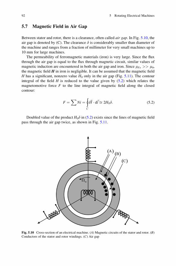
5.7 Magnetic Field in Air Gap
Between stator and rotor, there is a clearance, often called air gap. In Fig. 5.10, theair gap is denoted by (C). The clearance d is considerably smaller than diameter of
the machine and ranges from a fraction of millimeter for very small machines up to
10 mm for large machines.
The permeability of ferromagnetic materials (iron) is very large. Since the flux
through the air gap is equal to the flux through magnetic circuit, similar values of
magnetic induction are encountered in both the air gap and iron. Since mFe >> m0,the magnetic field H in iron is negligible. It can be assumed that the magnetic field
H has a significant, nonzero value H0 only in the air gap (Fig. 5.11). The contour
integral of the field H is reduced to the value given by (5.2) which relates the
magnetomotive force F to the line integral of magnetic field along the closed
contour:
F ¼X
Ni ¼þC
~H � d~l ffi 2H0d: (5.2)
Doubled value of the product H0d in (5.2) exists since the lines of magnetic field
pass through the air gap twice, as shown in Fig. 5.11.
Fig. 5.10 Cross-section of an electrical machine. (A) Magnetic circuits of the stator and rotor. (B)Conductors of the stator and rotor windings. (C) Air gap
92 5 Rotating Electrical Machines
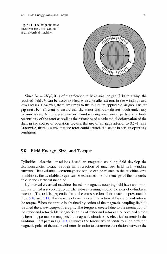
Since Ni ¼ 2H0d, it is of significance to have smaller gap d. In this way, the
required field H0 can be accomplished with a smaller current in the windings and
lower losses. However, there are limits to the minimum applicable air gap. The air
gap must be sufficient to ensure that the stator and rotor do not touch under any
circumstances. A finite precision in manufacturing mechanical parts and a finite
eccentricity of the rotor as well as the existence of elastic radial deformation of the
shaft in the course of operation prevent the use of air gaps inferior to 0.5–1 mm.
Otherwise, there is a risk that the rotor could scratch the stator in certain operating
conditions.
5.8 Field Energy, Size, and Torque
Cylindrical electrical machines based on magnetic coupling field develop the
electromagnetic torque through an interaction of magnetic field with winding
currents. The available electromagnetic torque can be related to the machine size.
In addition, the available torque can be estimated from the energy of the magnetic
field in the electrical machine.
Cylindrical electrical machines based on magnetic coupling field have an immo-
bile stator and a revolving rotor. The rotor is turning around the axis of cylindrical
machine. The axis is perpendicular to the cross-section of the machine presented in
Figs. 5.10 and 5.11. The measure of mechanical interaction of the stator and rotor is
the torque. When the torque is obtained by action of the magnetic coupling field, it
is called the electromagnetic torque. The torque is created due to the interaction of
the stator and rotor fields. Magnetic fields of stator and rotor can be obtained either
by inserting permanent magnets into magnetic circuit or by electrical currents in the
windings. Left part in Fig. 5.3 illustrates the torque which tends to align different
magnetic poles of the stator and rotor. In order to determine the relation between the
Fig. 5.11 The magnetic field
lines over the cross-section
of an electrical machine
5.8 Field Energy, Size, and Torque 93
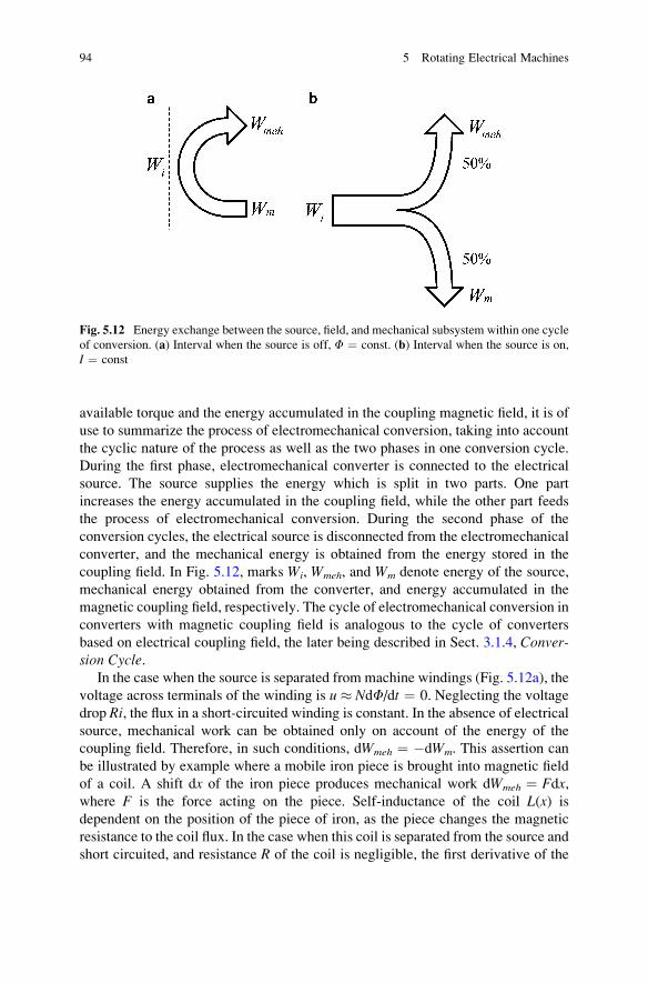
available torque and the energy accumulated in the coupling magnetic field, it is of
use to summarize the process of electromechanical conversion, taking into account
the cyclic nature of the process as well as the two phases in one conversion cycle.
During the first phase, electromechanical converter is connected to the electrical
source. The source supplies the energy which is split in two parts. One part
increases the energy accumulated in the coupling field, while the other part feeds
the process of electromechanical conversion. During the second phase of the
conversion cycles, the electrical source is disconnected from the electromechanical
converter, and the mechanical energy is obtained from the energy stored in the
coupling field. In Fig. 5.12, marks Wi, Wmeh, and Wm denote energy of the source,
mechanical energy obtained from the converter, and energy accumulated in the
magnetic coupling field, respectively. The cycle of electromechanical conversion in
converters with magnetic coupling field is analogous to the cycle of converters
based on electrical coupling field, the later being described in Sect. 3.1.4, Conver-sion Cycle.
In the case when the source is separated from machine windings (Fig. 5.12a), the
voltage across terminals of the winding is u � NdF/dt ¼ 0. Neglecting the voltage
drop Ri, the flux in a short-circuited winding is constant. In the absence of electricalsource, mechanical work can be obtained only on account of the energy of the
coupling field. Therefore, in such conditions, dWmeh ¼ �dWm. This assertion can
be illustrated by example where a mobile iron piece is brought into magnetic field
of a coil. A shift dx of the iron piece produces mechanical work dWmeh ¼ Fdx,where F is the force acting on the piece. Self-inductance of the coil L(x) is
dependent on the position of the piece of iron, as the piece changes the magnetic
resistance to the coil flux. In the case when this coil is separated from the source and
short circuited, and resistance R of the coil is negligible, the first derivative of the
Fig. 5.12 Energy exchange between the source, field, and mechanical subsystem within one cycle
of conversion. (a) Interval when the source is off, F ¼ const. (b) Interval when the source is on,
I ¼ const
94 5 Rotating Electrical Machines
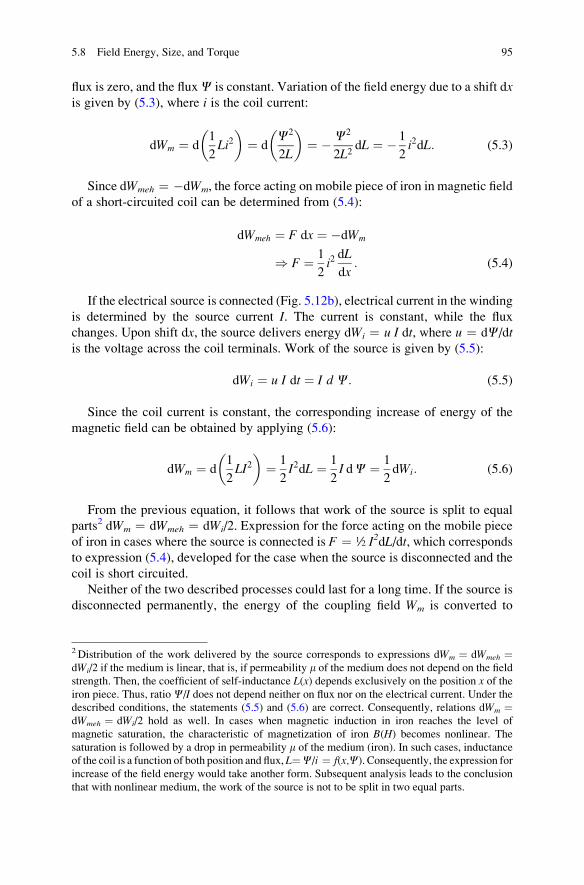
flux is zero, and the fluxC is constant. Variation of the field energy due to a shift dxis given by (5.3), where i is the coil current:
dWm ¼ d1
2Li2
� �¼ d
C2
2L
� �¼ � C2
2L2dL ¼ � 1
2i2dL: (5.3)
Since dWmeh ¼ �dWm, the force acting on mobile piece of iron in magnetic field
of a short-circuited coil can be determined from (5.4):
dWmeh ¼ F dx ¼ �dWm
) F ¼ 1
2i2dL
dx: (5.4)
If the electrical source is connected (Fig. 5.12b), electrical current in the winding
is determined by the source current I. The current is constant, while the flux
changes. Upon shift dx, the source delivers energy dWi ¼ u I dt, where u ¼ dC/dtis the voltage across the coil terminals. Work of the source is given by (5.5):
dWi ¼ u I dt ¼ I d C: (5.5)
Since the coil current is constant, the corresponding increase of energy of the
magnetic field can be obtained by applying (5.6):
dWm ¼ d1
2LI2
� �¼ 1
2I2dL ¼ 1
2I dC ¼ 1
2dWi: (5.6)
From the previous equation, it follows that work of the source is split to equal
parts2 dWm ¼ dWmeh ¼ dWi/2. Expression for the force acting on the mobile piece
of iron in cases where the source is connected is F ¼ ½ I2dL/dt, which correspondsto expression (5.4), developed for the case when the source is disconnected and the
coil is short circuited.
Neither of the two described processes could last for a long time. If the source is
disconnected permanently, the energy of the coupling field Wm is converted to
2Distribution of the work delivered by the source corresponds to expressions dWm ¼ dWmeh ¼dWi/2 if the medium is linear, that is, if permeability m of the medium does not depend on the field
strength. Then, the coefficient of self-inductance L(x) depends exclusively on the position x of theiron piece. Thus, ratioC/I does not depend neither on flux nor on the electrical current. Under the
described conditions, the statements (5.5) and (5.6) are correct. Consequently, relations dWm ¼dWmeh ¼ dWi/2 hold as well. In cases when magnetic induction in iron reaches the level of
magnetic saturation, the characteristic of magnetization of iron B(H) becomes nonlinear. The
saturation is followed by a drop in permeability m of the medium (iron). In such cases, inductance
of the coil is a function of both position and flux, L¼C/i ¼ f(x,C). Consequently, the expression for
increase of the field energy would take another form. Subsequent analysis leads to the conclusion
that with nonlinear medium, the work of the source is not to be split in two equal parts.
5.8 Field Energy, Size, and Torque 95
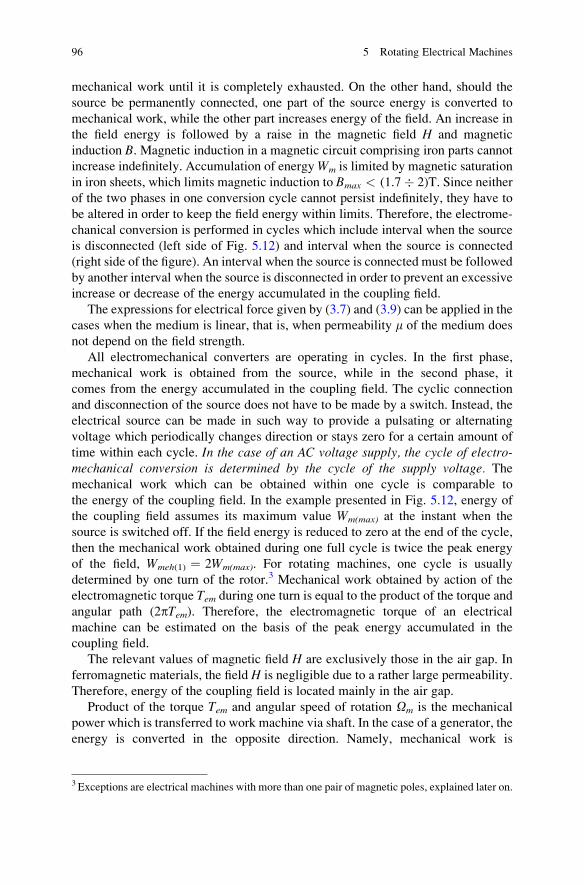
mechanical work until it is completely exhausted. On the other hand, should the
source be permanently connected, one part of the source energy is converted to
mechanical work, while the other part increases energy of the field. An increase in
the field energy is followed by a raise in the magnetic field H and magnetic
induction B. Magnetic induction in a magnetic circuit comprising iron parts cannot
increase indefinitely. Accumulation of energyWm is limited by magnetic saturation
in iron sheets, which limits magnetic induction to Bmax < (1.7 � 2)T. Since neither
of the two phases in one conversion cycle cannot persist indefinitely, they have to
be altered in order to keep the field energy within limits. Therefore, the electrome-
chanical conversion is performed in cycles which include interval when the source
is disconnected (left side of Fig. 5.12) and interval when the source is connected
(right side of the figure). An interval when the source is connected must be followed
by another interval when the source is disconnected in order to prevent an excessive
increase or decrease of the energy accumulated in the coupling field.
The expressions for electrical force given by (3.7) and (3.9) can be applied in the
cases when the medium is linear, that is, when permeability m of the medium does
not depend on the field strength.
All electromechanical converters are operating in cycles. In the first phase,
mechanical work is obtained from the source, while in the second phase, it
comes from the energy accumulated in the coupling field. The cyclic connection
and disconnection of the source does not have to be made by a switch. Instead, the
electrical source can be made in such way to provide a pulsating or alternating
voltage which periodically changes direction or stays zero for a certain amount of
time within each cycle. In the case of an AC voltage supply, the cycle of electro-mechanical conversion is determined by the cycle of the supply voltage. Themechanical work which can be obtained within one cycle is comparable to
the energy of the coupling field. In the example presented in Fig. 5.12, energy of
the coupling field assumes its maximum value Wm(max) at the instant when the
source is switched off. If the field energy is reduced to zero at the end of the cycle,
then the mechanical work obtained during one full cycle is twice the peak energy
of the field, Wmeh(1) ¼ 2Wm(max). For rotating machines, one cycle is usually
determined by one turn of the rotor.3 Mechanical work obtained by action of the
electromagnetic torque Tem during one turn is equal to the product of the torque and
angular path (2pTem). Therefore, the electromagnetic torque of an electrical
machine can be estimated on the basis of the peak energy accumulated in the
coupling field.
The relevant values of magnetic field H are exclusively those in the air gap. In
ferromagnetic materials, the field H is negligible due to a rather large permeability.
Therefore, energy of the coupling field is located mainly in the air gap.
Product of the torque Tem and angular speed of rotation Om is the mechanical
power which is transferred to work machine via shaft. In the case of a generator, the
energy is converted in the opposite direction. Namely, mechanical work is
3 Exceptions are electrical machines with more than one pair of magnetic poles, explained later on.
96 5 Rotating Electrical Machines
converted into electrical energy. Given the reference directions, the product of
generator torque Tem and speed Om is negative, indicating that the mechanical
power is transferred to electrical machine via shaft.
Question (5.2): If dimensions of a machine and the peak value of magnetic
induction are known, estimate the electromagnetic torque which can be developed
by this machine.
Answer (5.2): Energy accumulated in the electromagnetic field is located mainly
in the air gap. Volume of the air gap is V ¼ pLDd, where D is diameter of the
machine, L is axial length, and d is the air gap. Magnetic induction B in the air gap
depends on electrical current in the winding. Lines of the magnetic field which pass
through the air gap enter the ferromagnetic material. Usually, the ferromagnetic
parts are made of iron sheets which make up the stator and rotor magnetic circuits.
Therefore, induction in the air gap cannot exceed value Bmax � 1.7 T. Excessive
values of B would cause magnetic saturation in the iron sheets. Therefore, the
density of energy accumulated in magnetic field in the air gap cannot exceed ½
Bmax2/m0. The maximum energy of the coupling field can be estimated asWm(max) �
½ pLDdBmax2/m0, while the electromagnetic torque of the machine can be estimated
by dividing the obtained energy by 2p.
5.8 Field Energy, Size, and Torque 97
Chapter 6
Modeling Electrical Machines
This chapter introduces, develops and explains generalized mathematical model of
electrical machines. It explains the need for modeling, introduces and explains
approximations and neglected phenomena, and formulates generalized model as a
set of differential and algebraic equations.
Working with electrical machines requires mathematical representation of the
process of electromechanical conversion. It is necessary to determine equations
which correlate the electrical quantities of the machine, such as the voltages and
currents, with mechanical quantities such as the speed and torque. These equations
provide the link between the electrical access to the machine (terminals of the
windings) and the mechanical access to the machine (shaft). The two accesses to
the machine are shown in Fig. 6.1, which illustrates the process of electromechanical
conversions and presents the principal losses and the energy accumulated in mag-
netic field. Equations of the mathematical model are used to calculate changes in
electromagnetic torque, electromotive forces, currents, speed, and other relevant
variables. Besides, the model helps calculating conversion losses in windings, in
magnetic circuits, and in mechanical parts of the machine.
The set of equations describing transient processes in electrical machines
contains differential and algebraic equations, and it is also called dynamic model.Operation of a machine in steady states is described by the steady state equivalent
scheme, which gives relations between voltages and currents at the winding
terminals, and by mechanical characteristic, which describes relation between the
torque and speed at the mechanical access. In the following subsection, an intro-
duction to the modeling of electrical machines is presented. Figure 6.1 presents a
diagram showing power of the source Pe, mechanical power Pm, winding losses
PCu, losses in the coupling field PFe, mechanical losses due to rotation Pgm (motion
resistance losses), and energy of the coupling field Wm.
S.N. Vukosavic, Electrical Machines, Power Electronics and Power Systems,
DOI 10.1007/978-1-4614-0400-2_6, # Springer Science+Business Media New York 2013
99
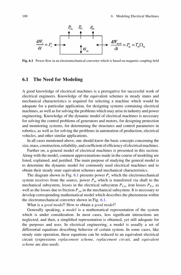
6.1 The Need for Modeling
A good knowledge of electrical machines is a prerogative for successful work of
electrical engineers. Knowledge of the equivalent schemes in steady states and
mechanical characteristics is required for selecting a machine which would be
adequate for a particular application, for designing systems containing electrical
machines, as well as for solving the problems which may arise in industry and power
engineering. Knowledge of the dynamic model of electrical machines is necessary
for solving the control problems of generators and motors, for designing protection
and monitoring systems, for determining the structures and control parameters in
robotics, as well as for solving the problems in automation of production, electrical
vehicles, and other similar applications.
In all cases mentioned above, one should know the basic concepts concerning the
size,mass, construction, reliability, and coefficient of efficiencyof electricalmachines.
Further on, a general model of electrical machines is presented in this section.
Along with the model, common approximations made in the course of modeling are
listed, explained, and justified. The main purpose of studying the general model is
to determine the dynamic model for commonly used electrical machines and to
obtain their steady state equivalent schemes and mechanical characteristics.
The diagram shown in Fig. 6.1 presents power Pe which the electromechanical
system receives from the source, power Pm which is transferred via shaft to the
mechanical subsystem, losses in the electrical subsystem PCu, iron losses PFe, as
well as the losses due to friction Pgm in the mechanical subsystem. It is necessary to
develop corresponding mathematical model which describes the phenomena within
the electromechanical converter shown in Fig. 6.1.
What is a good model? How to obtain a good model?Generally speaking, a model is a mathematical representation of the system
which is under consideration. In most cases, less significant interactions are
neglected, and then, a simplified representation is obtained, yet still adequate for
the purposes and uses. In electrical engineering, a model is usually a set of
differential equations describing behavior of certain system. In some cases, like
steady state operation, these equations can be reduced to an equivalent electrical
circuit (expressions replacement scheme, replacement circuit, and equivalentscheme are also used).
Fig. 6.1 Power flow in an electromechanical converter which is based on magnetic coupling field
100 6 Modeling Electrical Machines
The phenomena and systems of interest for an electrical engineer are usually
complex and include some interactions which are not of uttermost importance and
should not be taken into account. Considering gas pressure pushing the head of a
piston in the cylinder of an endothermic motor, the action is the result of continuous
collisions of a large number of gas particles with the surface of the piston. Strictly
speaking, the force is not constant, but it consists of a very large number of strikes
(pulses) per second. However, in the analysis of the torque which the motor transfers
to the work machine, only the average value of the force is of interest. Therefore, the
effects of micro strikes are neglected, and the force is considered to be proportional
to the surface of the piston head and to the gas pressure in the cylinder.
In electrical engineering, passive components, such as resistors, capacitors, and
inductive coils (chokes), are very often mentioned and used. Strictly speaking,
models of real chokes, capacitors, and resistors are more complex compared to
widely accepted models that are rather simple. At high frequencies, influences of
parasitic inductance and equivalent series resistance of a capacitor become notice-
able. Under similar conditions, parallel capacitance of a choke cannot be neglected
at very high frequencies. Similar conclusion can be made for a resistor. In a rigorous
analysis, real components would have to be modeled as networks with distributed
parameter. Yet the frequencies of interest are often low. At low frequencies,
parasitic effects are negligible, and the well-known elements R, L, and C are
considered as lumped parameter circuit elements described by relations Ri ¼ u,u ¼ Ldi/dt, and i ¼ Cdu/dt. Therefore, parasitic effects and distributed parameters
do not have to be taken into account when solving problems and tasks at low
frequencies. In cases when all the parasitic and secondary effects are modeled, the
considered RLC networks become rather complex, and their analysis becomes
difficult. Drawing conclusions or making design decisions based upon too complex
models becomes virtually impossible.
Therefore, a good model is not the one that takes into account all aspects of
dynamic behavior of a system, but the one which is simplified by justifiable
approximations, thus facilitating and improving the process of making conclusions
and taking design decisions, while retaining all relevant (significant) phenomena
within the system. It is not possible to develop an analytical expression which
would help in defining the relevance, but in making approximations, it is necessary
to distinguish the essential from nonessential on the basis of a deeper knowledge of
the system and material and through the use of experience. A tip to apprentices in
modeling conventional electrical machines is to take into account all the phenom-
ena up to several tens of kHz and to neglect the processes at higher frequencies.
6.1.1 Problems of Modeling
In the process of modeling, it is required to neglect insignificant phenomena in
order to obtain a simple, clear-cut, and usable model. For successful modeling and
use of the model, it is necessary to make correct judgment as regards phenomena
6.1 The Need for Modeling 101
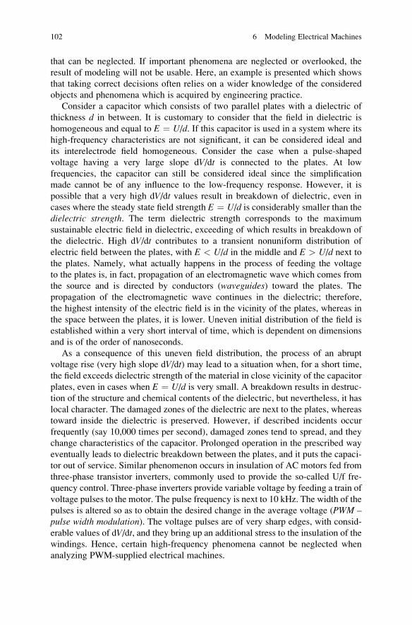
that can be neglected. If important phenomena are neglected or overlooked, the
result of modeling will not be usable. Here, an example is presented which shows
that taking correct decisions often relies on a wider knowledge of the considered
objects and phenomena which is acquired by engineering practice.
Consider a capacitor which consists of two parallel plates with a dielectric of
thickness d in between. It is customary to consider that the field in dielectric is
homogeneous and equal to E ¼ U/d. If this capacitor is used in a system where its
high-frequency characteristics are not significant, it can be considered ideal and
its interelectrode field homogeneous. Consider the case when a pulse-shaped
voltage having a very large slope dV/dt is connected to the plates. At low
frequencies, the capacitor can still be considered ideal since the simplification
made cannot be of any influence to the low-frequency response. However, it is
possible that a very high dV/dt values result in breakdown of dielectric, even in
cases where the steady state field strength E ¼ U/d is considerably smaller than the
dielectric strength. The term dielectric strength corresponds to the maximum
sustainable electric field in dielectric, exceeding of which results in breakdown of
the dielectric. High dV/dt contributes to a transient nonuniform distribution of
electric field between the plates, with E < U/d in the middle and E > U/d next to
the plates. Namely, what actually happens in the process of feeding the voltage
to the plates is, in fact, propagation of an electromagnetic wave which comes from
the source and is directed by conductors (waveguides) toward the plates. The
propagation of the electromagnetic wave continues in the dielectric; therefore,
the highest intensity of the electric field is in the vicinity of the plates, whereas in
the space between the plates, it is lower. Uneven initial distribution of the field is
established within a very short interval of time, which is dependent on dimensions
and is of the order of nanoseconds.
As a consequence of this uneven field distribution, the process of an abrupt
voltage rise (very high slope dV/dt) may lead to a situation when, for a short time,
the field exceeds dielectric strength of the material in close vicinity of the capacitor
plates, even in cases when E ¼ U/d is very small. A breakdown results in destruc-
tion of the structure and chemical contents of the dielectric, but nevertheless, it has
local character. The damaged zones of the dielectric are next to the plates, whereas
toward inside the dielectric is preserved. However, if described incidents occur
frequently (say 10,000 times per second), damaged zones tend to spread, and they
change characteristics of the capacitor. Prolonged operation in the prescribed way
eventually leads to dielectric breakdown between the plates, and it puts the capaci-
tor out of service. Similar phenomenon occurs in insulation of AC motors fed from
three-phase transistor inverters, commonly used to provide the so-called U/f fre-
quency control. Three-phase inverters provide variable voltage by feeding a train of
voltage pulses to the motor. The pulse frequency is next to 10 kHz. The width of the
pulses is altered so as to obtain the desired change in the average voltage (PWM –pulse width modulation). The voltage pulses are of very sharp edges, with consid-
erable values of dV/dt, and they bring up an additional stress to the insulation of thewindings. Hence, certain high-frequency phenomena cannot be neglected when
analyzing PWM-supplied electrical machines.
102 6 Modeling Electrical Machines
The example considered above requires a deeper understanding of the process
and is founded on experience. The knowledge required for thorough understanding
of given example is not a prerequisite for further reading. However, it is of interest
to recognize the need to enrich the studies by laboratory work, practice, written
papers, and projects, acquiring in this way the experience necessary for a successful
engineering practice. A successful engineer combines the theoretical knowledge,
skill in solving analytically solvable problems, but also the experience in modeling
processes and phenomena. In order to make the most out of the knowledge and skill,
it is necessary primarily to use the experience and deeper understanding of the
process of electromechanical conversion and reduce a complex system to a mathe-
matical model to be used in further work.
6.1.2 Conclusion
A good model is the simplest possible model still representing the relevant aspects
of the dynamic behavior of a system – process – machine in a satisfactory way.
In the process of generating models, justifiable approximations are made in order
to make a simple model suitable for recognizing relevant and significant phenom-
ena, for making conclusions, and for taking engineering and design decisions.
When introducing the approximations, care should be taken that these do not
jeopardize the accuracy to the extent that makes the model useless.
This book is the first encounter with cylindrical electromechanical converters
with magnetic coupling field for a number of readers. Therefore, initial steps in
machine analysis and modeling are made with certain approximations. Among the
four principal approximations, the losses in magnetic circuits or iron losses are also
neglected. Omission of these losses makes the basic models of electrical machines
easier to understand. In most electrical machines, iron losses are marginalized by
lamination, and the mentioned approximation is partially justifiable. It is necessary,
however, to have in mind that at higher frequencies and larger magnetic induction,
the iron losses can be considerable and should be taken into account in calculating
the total losses and coefficient of efficiency, as well as in designing the corres-
ponding cooling systems.
6.2 Neglected Phenomena
In the course of developing a model, it is justifiable to neglect less significant
phenomena, the omission of which does not cause significant deviations of the
obtained results. The four most common approximations are:
• The system is considered as a lumped parameter network.
• Parasitic capacitances are neglected.
6.2 Neglected Phenomena 103
• The iron losses are neglected.
• Ferromagnetic materials are considered linear
6.2.1 Distributed Energy and Distributed Parameters
Electrical machines are usually considered as networks with lumped parameters
and represented by circuits comprising discrete inductances and resistances. Con-
sidering actual L and C elements, the coil energy resides in spatially distributed
magnetic field, while the capacitor energy resides in spatially distributed electrical
field. It is well known1 that changes in magnetic field give a rise to induced
electrical field and vice versa. The induced field is proportional to the rate of changeof the inducting field, that is, to the operating frequency. Hence, a coil with an AC
current is surrounded by magnetic field, but also with an induced electrical field, the
strength of which depends on the operating frequency. Similar conclusion can be
drawn for a capacitor. The presence of both fields contributes to parasitic capaci-
tance of the coil and parasitic inductance of the capacitor.
Lumped parameter approach neglects the spatial distribution of the coil and
capacitor energy. It is assumed that both energies reside within discrete elements
and that the amounts ½Li2 and ½Cu2 do not reside in space. The coils and capacitorsare considered ideal, lumped parameter L-C elements. The adopted models are
uL ¼ Ldi/dt and iC ¼ Cdu/dt, neglecting the secondary effects such as capacitance
of a coil or inductance of a capacitor. With the induced fields being proportional
to the operating frequency, lumped parameter approach introduces a negligible error
at relatively low frequencies that are in use in typical applications of electrical
machines.
One of the consequences of neglecting distributed energy and distributed
parameters is concealing the energy transfer. In a lumped parameter network, a
pair of conductors with electrical current i and voltage u transmits the energy at
a rate of p ¼ ui. This expression involves macroscopic quantities like voltage and
current and suggests that the energy passes through conductors. In reality, the
energy is transmitted through the surrounding space with the presence of electrical
and magnetic field.
6.2.2 Neglecting Parasitic Capacitances
For electrical machines operating on the basis of a magnetic coupling field, the
effects of parasitic capacitances of the windings and the amounts of energy
accumulated in the electrical field are negligible. Since the spatial density of
1 Consider Maxwell equations, such as rot ~E ¼ �@~B=@t:
104 6 Modeling Electrical Machines
magnetic field is considerably higher than that of electrical field (mH2 » eE2), it is
justified to neglect the capacitances between insulated conductors and capacitances
between the windings and magnetic circuit.
6.2.3 Neglecting Iron Losses
It is considered that the losses due to hysteresis and losses due to eddy currents are
considerably smaller compared to the power of conversion; thus, they can be
neglected. Specific losses in ferromagnetic materials (iron losses) are dependent
on magnetic induction and operating frequency and they can be represented by the
following expression:
pFe ¼PFe
m¼ pH þ pV ¼ sH � f � Bm
2 þ sV � f 2 � Bm2:
Since the losses due to eddy currents are dependent on squared frequency and
squared magnetic induction, the iron losses are to be reconsidered in cases when
electrical machine operates with elevated frequencies. In such cases, it is necessary
to check whether neglecting the iron losses can be justified.
6.2.4 Neglecting Iron Nonlinearity
The characteristic of magnetization of magnetic materials is considered linear.
Therefore, the effects of saturation of the ferromagnetic material (iron) are neglected.
PermeabilityB/H is considered constant and equal to differential permeabilityDB/DHat all operating points of the magnetization characteristic. In applications where
induction exceeds 1.2T, it is necessary to check whether this is justified.
General model of electrical machine based onmagnetic coupling field is developed
hereafter relying on the four basic approximationsmentioned above. It is assumed that
the converter has N windings which can be either short-circuited or connected to a
source. The windings are mounted on the rotor or stator.
6.3 Power of Electrical Sources
Figure 6.2 shows a converter having N magnetically coupled contours (windings)
which could be either connected to a power source or separated from it and brought
into short circuit. Windings of electrical machines can be fed from current or
voltage sources. Real voltage sources have finite internal resistance (impedance),
whereas current sources have finite internal conductance (admittance). With no loss
in generality, in further text, it is assumed that electrical sources are ideal.
6.3 Power of Electrical Sources 105
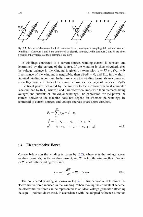
In windings connected to a current source, winding current is constant and
determined by the current of the source. If the winding is short-circuited, then
the voltage balance in the winding is given by expression u ¼ Ri + dC/dt ¼ 0.
If resistance of the winding is negligible, then dC/dt ¼ 0, and flux in the short-
circuited winding is constant. In the case where the winding terminals are connected
to a voltage source, voltage of the source determines the change of flux (u� dC/dt).Electrical power delivered by the sources to the electromechanical converter
is determined by (6.1), where u and i are vector-columns with their elements being
voltages and currents of individual windings. The expression for the power the
sources deliver to the machine does not depend on whether the windings are
connected to current sources and voltage sources or are short-circuited.
Pe ¼XNj¼1
ujij ¼ iT � u;
iT ¼ ½i1; i2; . . . ii; . . . iN�1; iN�;uT ¼ ½u1; u2; . . . ui; . . . uN�1; uN�: (6.1)
6.4 Electromotive Force
Voltage balance in the winding is given by (6.2), where u is the voltage across
winding terminals, i is the winding current, andC¼NF is the winding flux. Parame-
ter R denotes the winding resistance.
u ¼ Riþ dCdt
¼ Riþ eCEMF (6.2)
The considered winding is shown in Fig. 6.3. Flux derivative determines the
electromotive force induced in the winding. When making the equivalent scheme,
the electromotive force can be represented as an ideal voltage generator attaching
the sign þ pointed downward, in accordance with the adopted reference direction
Fig. 6.2 Model of electromechanical converter based on magnetic coupling field with N contours
(windings). Contours 1 and i are connected to electric sources, while contours 2 and N are short
circuited thus voltages at their terminals are zero
106 6 Modeling Electrical Machines
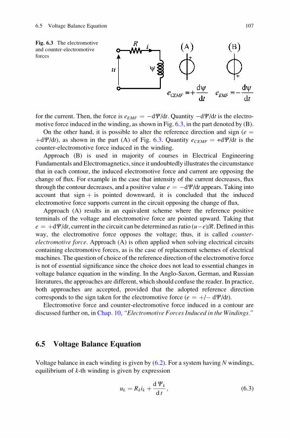
for the current. Then, the force is eEMF ¼ �dC/dt. Quantity �dC/dt is the electro-motive force induced in the winding, as shown in Fig. 6.3, in the part denoted by (B).
On the other hand, it is possible to alter the reference direction and sign (e ¼þdC/dt), as shown in the part (A) of Fig. 6.3. Quantity eCEMF ¼ +dC/dt is the
counter-electromotive force induced in the winding.
Approach (B) is used in majority of courses in Electrical Engineering
Fundamentals and Electromagnetics, since it undoubtedly illustrates the circumstance
that in each contour, the induced electromotive force and current are opposing the
change of flux. For example in the case that intensity of the current decreases, flux
through the contour decreases, and a positive value e ¼ �dC/dt appears. Taking intoaccount that sign þ is pointed downward, it is concluded that the induced
electromotive force supports current in the circuit opposing the change of flux.
Approach (A) results in an equivalent scheme where the reference positive
terminals of the voltage and electromotive force are pointed upward. Taking that
e ¼ þdC/dt, current in the circuit can be determined as ratio (u – e)/R. Defined in thisway, the electromotive force opposes the voltage; thus, it is called counter-electromotive force. Approach (A) is often applied when solving electrical circuits
containing electromotive forces, as is the case of replacement schemes of electrical
machines. The question of choice of the reference direction of the electromotive force
is not of essential significance since the choice does not lead to essential changes in
voltage balance equation in the winding. In the Anglo-Saxon, German, and Russian
literatures, the approaches are different, which should confuse the reader. In practice,
both approaches are accepted, provided that the adopted reference direction
corresponds to the sign taken for the electromotive force (e ¼ þ/� dC/dt).Electromotive force and counter-electromotive force induced in a contour are
discussed further on, in Chap. 10, “Electromotive Forces Induced in the Windings.”
6.5 Voltage Balance Equation
Voltage balance in each winding is given by (6.2). For a system having N windings,
equilibrium of k-th winding is given by expression
uk ¼ Rkik þ dCk
d t; (6.3)
Fig. 6.3 The electromotive
and counter-electromotive
forces
6.5 Voltage Balance Equation 107
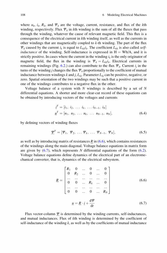
where uk, ik, Rk, and Ck are the voltage, current, resistance, and flux of the kthwinding, respectively. Flux Ck in kth winding is the sum of all the fluxes that pass
through the winding, whatever the cause of relevant magnetic field. This flux is a
consequence of the electrical current in kth winding itself, as well as the currents inother windings that are magnetically coupled to k-th winding. The part of the flux
Ck caused by the current ik is equal to Lkkik. The coefficient Lkk is also called self-inductance of the winding. Self-inductance is expressed in H ¼ Wb/A, and it is
strictly positive. In cases where the current in the winding ik is the only originator ofmagnetic field, the flux in the winding is Ck ¼ Lkkik. Electrical currents in
remaining windings (Fig. 6.2.) can also contribute to the flux Ck. Current ij in the
turns of the winding j changes the fluxCk proportionally to the coefficient of mutual
inductance between windings k and j, Lkj. Parameter Lkj can be positive, negative, orzero. Spatial orientation of the two windings may be such that a positive current in
one of the windings contributes to a negative flux in the other.
Voltage balance of a system with N windings is described by a set of Ndifferential equations. A shorter and more clear-cut record of these equations can
be obtained by introducing vectors of the voltages and currents
iT ¼ ½i1; i2; . . . ik; . . . iN�1; iN�uT ¼ ½u1; u2; . . . uk; . . . uN�1; uN�; (6.4)
by defining vectors of winding fluxes
CT ¼ ½C1; C2; . . . Ck; . . . CN�1; CN�; (6.5)
as well as by introducing matrix of resistances R in (6.6), which contains resistances
of the windings along the main diagonal. Voltage balance equations in matrix form
are given by (6.7), which represents N differential equations of the form (6.2).
Voltage balance equations define dynamics of the electrical part of an electrome-
chanical converter, that is, dynamics of the electrical subsystem.
R ¼
R1 0 ::: 0 ::: 0
0 R2 ::: 0 ::: 0
::: ::: ::: ::: ::: :::0 0 ::: Rk ::: 0
::: ::: ::: ::: ::: :::0 0 ::: 0 ::: RN
26666664
37777775
(6.6)
u ¼ R � iþ dCdt
(6.7)
Flux vector-column C is determined by the winding currents, self-inductances,
and mutual inductances. Flux of kth winding is determined by the coefficient of
self-inductance of the winding k, as well as by the coefficients of mutual inductance
108 6 Modeling Electrical Machines
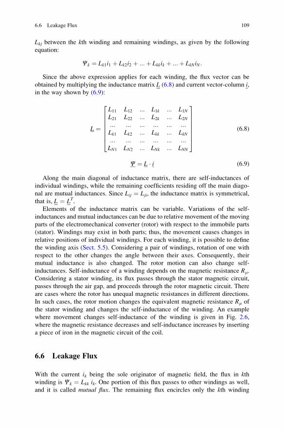
Lkj between the kth winding and remaining windings, as given by the following
equation:
Ck ¼ Lk1i1 þ Lk2i2 þ ::: þ Lkkik þ :::þ LkNiN:
Since the above expression applies for each winding, the flux vector can be
obtained by multiplying the inductance matrix L (6.8) and current vector-column i,in the way shown by (6.9):
L ¼
L11 L12 ::: L1k ::: L1NL21 L22 ::: L2k ::: L2N::: ::: ::: ::: ::: :::Lk1 Lk2 ::: Lkk ::: LkN::: ::: ::: ::: ::: :::LN1 LN2 ::: LNk ::: LNN
26666664
37777775
(6.8)
C ¼ L � i (6.9)
Along the main diagonal of inductance matrix, there are self-inductances of
individual windings, while the remaining coefficients residing off the main diago-
nal are mutual inductances. Since Lij ¼ Lji, the inductance matrix is symmetrical,
that is, L ¼ LT.Elements of the inductance matrix can be variable. Variations of the self-
inductances and mutual inductances can be due to relative movement of the moving
parts of the electromechanical converter (rotor) with respect to the immobile parts
(stator). Windings may exist in both parts; thus, the movement causes changes in
relative positions of individual windings. For each winding, it is possible to define
the winding axis (Sect. 5.5). Considering a pair of windings, rotation of one with
respect to the other changes the angle between their axes. Consequently, their
mutual inductance is also changed. The rotor motion can also change self-
inductances. Self-inductance of a winding depends on the magnetic resistance Rm.
Considering a stator winding, its flux passes through the stator magnetic circuit,
passes through the air gap, and proceeds through the rotor magnetic circuit. There
are cases where the rotor has unequal magnetic resistances in different directions.
In such cases, the rotor motion changes the equivalent magnetic resistance Rm of
the stator winding and changes the self-inductance of the winding. An example
where movement changes self-inductance of the winding is given in Fig. 2.6,
where the magnetic resistance decreases and self-inductance increases by inserting
a piece of iron in the magnetic circuit of the coil.
6.6 Leakage Flux
With the current ik being the sole originator of magnetic field, the flux in kthwinding is Ck ¼ Lkk ik. One portion of this flux passes to other windings as well,
and it is called mutual flux. The remaining flux encircles only the kth winding
6.6 Leakage Flux 109
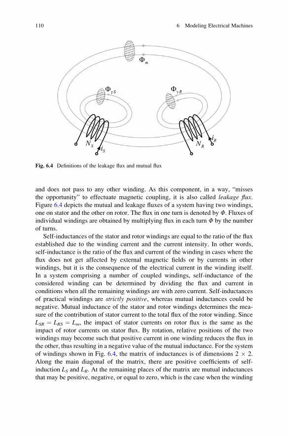
and does not pass to any other winding. As this component, in a way, “misses
the opportunity” to effectuate magnetic coupling, it is also called leakage flux.Figure 6.4 depicts the mutual and leakage fluxes of a system having two windings,
one on stator and the other on rotor. The flux in one turn is denoted by F. Fluxes ofindividual windings are obtained by multiplying flux in each turn F by the number
of turns.
Self-inductances of the stator and rotor windings are equal to the ratio of the flux
established due to the winding current and the current intensity. In other words,
self-inductance is the ratio of the flux and current of the winding in cases where the
flux does not get affected by external magnetic fields or by currents in other
windings, but it is the consequence of the electrical current in the winding itself.
In a system comprising a number of coupled windings, self-inductance of the
considered winding can be determined by dividing the flux and current in
conditions when all the remaining windings are with zero current. Self-inductances
of practical windings are strictly positive, whereas mutual inductances could be
negative. Mutual inductance of the stator and rotor windings determines the mea-
sure of the contribution of stator current to the total flux of the rotor winding. Since
LSR ¼ LRS ¼ Lm, the impact of stator currents on rotor flux is the same as the
impact of rotor currents on stator flux. By rotation, relative positions of the two
windings may become such that positive current in one winding reduces the flux in
the other, thus resulting in a negative value of the mutual inductance. For the system
of windings shown in Fig. 6.4, the matrix of inductances is of dimensions 2 � 2.
Along the main diagonal of the matrix, there are positive coefficients of self-
induction LS and LR. At the remaining places of the matrix are mutual inductances
that may be positive, negative, or equal to zero, which is the case when the winding
Fig. 6.4 Definitions of the leakage flux and mutual flux
110 6 Modeling Electrical Machines
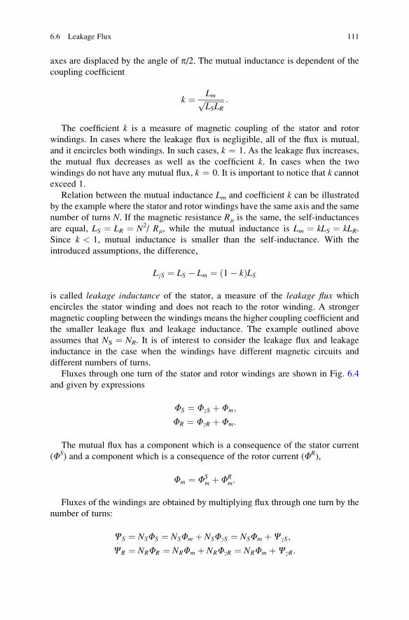
axes are displaced by the angle of p/2. The mutual inductance is dependent of the
coupling coefficient
k ¼ LmffiffiffiffiffiffiffiffiffiffiLSLR
p :
The coefficient k is a measure of magnetic coupling of the stator and rotor
windings. In cases where the leakage flux is negligible, all of the flux is mutual,
and it encircles both windings. In such cases, k ¼ 1. As the leakage flux increases,
the mutual flux decreases as well as the coefficient k. In cases when the two
windings do not have any mutual flux, k ¼ 0. It is important to notice that k cannotexceed 1.
Relation between the mutual inductance Lm and coefficient k can be illustrated
by the example where the stator and rotor windings have the same axis and the same
number of turns N. If the magnetic resistance Rm is the same, the self-inductances
are equal, LS ¼ LR ¼ N2/ Rm, while the mutual inductance is Lm ¼ kLS ¼ kLR.Since k < 1, mutual inductance is smaller than the self-inductance. With the
introduced assumptions, the difference,
LgS ¼ LS � Lm ¼ ð1� kÞLS
is called leakage inductance of the stator, a measure of the leakage flux which
encircles the stator winding and does not reach to the rotor winding. A stronger
magnetic coupling between the windings means the higher coupling coefficient and
the smaller leakage flux and leakage inductance. The example outlined above
assumes that NS ¼ NR. It is of interest to consider the leakage flux and leakage
inductance in the case when the windings have different magnetic circuits and
different numbers of turns.
Fluxes through one turn of the stator and rotor windings are shown in Fig. 6.4
and given by expressions
FS ¼ FgS þ Fm;
FR ¼ FgR þ Fm:
The mutual flux has a component which is a consequence of the stator current
(FS) and a component which is a consequence of the rotor current (FR),
Fm ¼ FSm þ FR
m:
Fluxes of the windings are obtained by multiplying flux through one turn by the
number of turns:
CS ¼ NSFS ¼ NSFm þ NSFgS ¼ NSFm þCgS;
CR ¼ NRFR ¼ NRFm þ NRFgR ¼ NRFm þCgR:
6.6 Leakage Flux 111
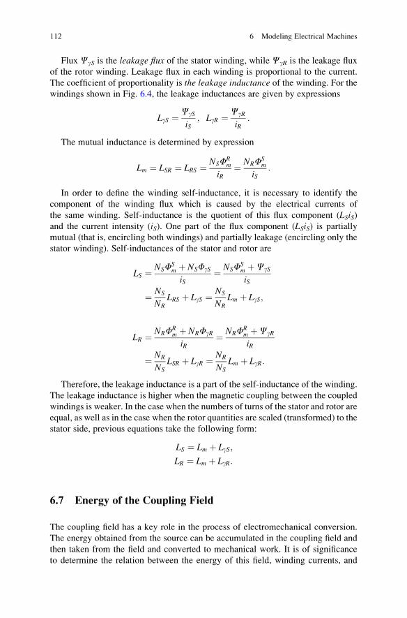
Flux CgS is the leakage flux of the stator winding, while CgR is the leakage flux
of the rotor winding. Leakage flux in each winding is proportional to the current.
The coefficient of proportionality is the leakage inductance of the winding. For thewindings shown in Fig. 6.4, the leakage inductances are given by expressions
LgS ¼ CgS
iS; LgR ¼ CgR
iR:
The mutual inductance is determined by expression
Lm ¼ LSR ¼ LRS ¼ NSFRm
iR¼ NRFS
m
iS:
In order to define the winding self-inductance, it is necessary to identify the
component of the winding flux which is caused by the electrical currents of
the same winding. Self-inductance is the quotient of this flux component (LSiS)and the current intensity (iS). One part of the flux component (LSiS) is partially
mutual (that is, encircling both windings) and partially leakage (encircling only the
stator winding). Self-inductances of the stator and rotor are
LS ¼ NSFSm þ NSFgS
iS¼ NSFS
m þCgS
iS
¼ NS
NRLRS þ LgS ¼ NS
NRLm þ LgS;
LR ¼ NRFRm þ NRFgR
iR¼ NRFR
m þCgR
iR
¼ NR
NSLSR þ LgR ¼ NR
NSLm þ LgR:
Therefore, the leakage inductance is a part of the self-inductance of the winding.
The leakage inductance is higher when the magnetic coupling between the coupled
windings is weaker. In the case when the numbers of turns of the stator and rotor are
equal, as well as in the case when the rotor quantities are scaled (transformed) to the
stator side, previous equations take the following form:
LS ¼ Lm þ LgS;
LR ¼ Lm þ LgR:
6.7 Energy of the Coupling Field
The coupling field has a key role in the process of electromechanical conversion.
The energy obtained from the source can be accumulated in the coupling field and
then taken from the field and converted to mechanical work. It is of significance
to determine the relation between the energy of this field, winding currents, and
112 6 Modeling Electrical Machines
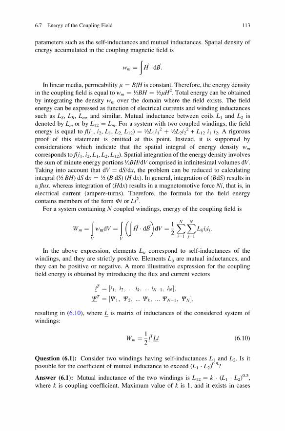
parameters such as the self-inductances and mutual inductances. Spatial density of
energy accumulated in the coupling magnetic field is
wm ¼ð~H � d~B:
In linear media, permeability m ¼ B/H is constant. Therefore, the energy density
in the coupling field is equal to wm ¼ ½BH ¼ ½mH2. Total energy can be obtained
by integrating the density wm over the domain where the field exists. The field
energy can be expressed as function of electrical currents and winding inductances
such as LS, LR, Lm, and similar. Mutual inductance between coils L1 and L2 is
denoted by Lm or by L12 ¼ Lm. For a system with two coupled windings, the field
energy is equal to f(i1, i2, L1, L2, L12) ¼ ½L1i12 þ ½L2i2
2 + L12 i1 i2. A rigorous
proof of this statement is omitted at this point. Instead, it is supported by
considerations which indicate that the spatial integral of energy density wm
corresponds to f(i1, i2, L1, L2, L12). Spatial integration of the energy density involvesthe sum of minute energy portions ½BH/dV comprised in infinitesimal volumes dV.Taking into account that dV ¼ dS/dx, the problem can be reduced to calculating
integral (½ BH) dS dx ¼ ½ (B dS) (H dx). In general, integration of (BdS) results ina flux, whereas integration of (Hdx) results in a magnetomotive force Ni, that is, inelectrical current (ampere-turns). Therefore, the formula for the field energy
contains members of the form Fi or Li2.For a system containing N coupled windings, energy of the coupling field is
Wm ¼ðV
wmdV ¼ðV
ð~H � d~B
� �dV ¼ 1
2
XNi¼1
XNj¼1
Lijiiij:
In the above expression, elements Lii correspond to self-inductances of the
windings, and they are strictly positive. Elements Lij are mutual inductances, and
they can be positive or negative. A more illustrative expression for the coupling
field energy is obtained by introducing the flux and current vectors
iT ¼ i1; i2; ::: ik; ::: iN�1; iN½ �;CT ¼ C1; C2; ::: Ck; ::: CN�1; CN½ �;
resulting in (6.10), where L is matrix of inductances of the considered system of
windings:
Wm ¼ 1
2iTLi (6.10)
Question (6.1): Consider two windings having self-inductances L1 and L2. Is it
possible for the coefficient of mutual inductance to exceed (L1 � L2)0.5?Answer (6.1): Mutual inductance of the two windings is L12 ¼ k � (L1 � L2)0.5,where k is coupling coefficient. Maximum value of k is 1, and it exists in cases
6.7 Energy of the Coupling Field 113
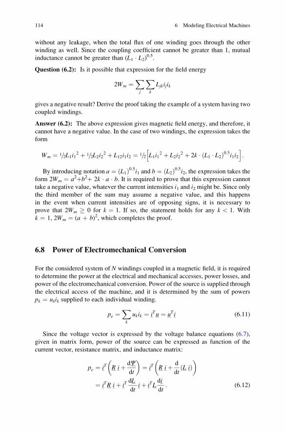
without any leakage, when the total flux of one winding goes through the other
winding as well. Since the coupling coefficient cannot be greater than 1, mutual
inductance cannot be greater than (L1 � L2)0.5.Question (6.2): Is it possible that expression for the field energy
2Wm ¼Xj
Xk
Ljkijik
gives a negative result? Derive the proof taking the example of a system having two
coupled windings.
Answer (6.2): The above expression gives magnetic field energy, and therefore, it
cannot have a negative value. In the case of two windings, the expression takes the
form
Wm ¼ 1=2L1i12 þ 1=2L2i2
2 þ L12i1i2 ¼ 1=2 L1i12 þ L2i2
2 þ 2k � ðL1 � L2Þ0:5i1i2h i
:
By introducing notation a ¼ ðL1Þ0:5i1 and b ¼ ðL2Þ0:5i2, the expression takes the
form 2Wm ¼ a2þb2þ 2k � a � b. It is required to prove that this expression cannot
take a negative value, whatever the current intensities i1 and i2 might be. Since only
the third member of the sum may assume a negative value, and this happens
in the event when current intensities are of opposing signs, it is necessary to
prove that 2Wm � 0 for k ¼ 1. If so, the statement holds for any k < 1. With
k ¼ 1, 2Wm ¼ (a þ b)2, which completes the proof.
6.8 Power of Electromechanical Conversion
For the considered system of N windings coupled in a magnetic field, it is required
to determine the power at the electrical and mechanical accesses, power losses, and
power of the electromechanical conversion. Power of the source is supplied through
the electrical access of the machine, and it is determined by the sum of powers
pk ¼ ukik supplied to each individual winding.
pe ¼Xk
ukik ¼ iTu ¼ uTi (6.11)
Since the voltage vector is expressed by the voltage balance equations (6.7),
given in matrix form, power of the source can be expressed as function of the
current vector, resistance matrix, and inductance matrix:
pe ¼ iT R iþ dCdt
� �¼ iT R iþ d
dtðL iÞ
� �
¼ iTR iþ iTdL
dtiþ iTL
di
dt: (6.12)
114 6 Modeling Electrical Machines
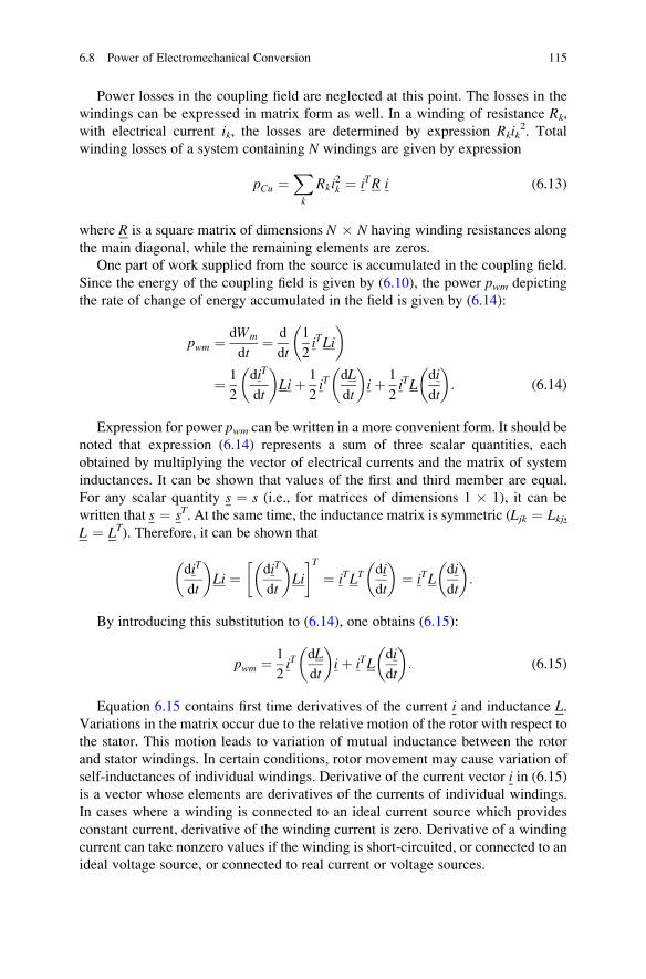
Power losses in the coupling field are neglected at this point. The losses in the
windings can be expressed in matrix form as well. In a winding of resistance Rk,
with electrical current ik, the losses are determined by expression Rkik2. Total
winding losses of a system containing N windings are given by expression
pCu ¼Xk
Rki2k ¼ iTR i (6.13)
where R is a square matrix of dimensions N � N having winding resistances along
the main diagonal, while the remaining elements are zeros.
One part of work supplied from the source is accumulated in the coupling field.
Since the energy of the coupling field is given by (6.10), the power pwm depicting
the rate of change of energy accumulated in the field is given by (6.14):
pwm ¼ dWm
dt¼ d
dt
1
2iTLi
� �
¼ 1
2
diT
dt
� �Liþ 1
2iT
dL
dt
� �iþ 1
2iTL
di
dt
� �: (6.14)
Expression for power pwm can be written in a more convenient form. It should be
noted that expression (6.14) represents a sum of three scalar quantities, each
obtained by multiplying the vector of electrical currents and the matrix of system
inductances. It can be shown that values of the first and third member are equal.
For any scalar quantity s ¼ s (i.e., for matrices of dimensions 1 � 1), it can be
written that s ¼ sT. At the same time, the inductance matrix is symmetric (Ljk ¼ Lkj,L ¼ LT). Therefore, it can be shown that
diT
dt
� �Li ¼ diT
dt
� �Li
� �T¼ iTLT
di
dt
� �¼ iTL
di
dt
� �:
By introducing this substitution to (6.14), one obtains (6.15):
pwm ¼ 1
2iT
dL
dt
� �iþ iTL
di
dt
� �: (6.15)
Equation 6.15 contains first time derivatives of the current i and inductance L.Variations in the matrix occur due to the relative motion of the rotor with respect to
the stator. This motion leads to variation of mutual inductance between the rotor
and stator windings. In certain conditions, rotor movement may cause variation of
self-inductances of individual windings. Derivative of the current vector i in (6.15)
is a vector whose elements are derivatives of the currents of individual windings.
In cases where a winding is connected to an ideal current source which provides
constant current, derivative of the winding current is zero. Derivative of a winding
current can take nonzero values if the winding is short-circuited, or connected to an
ideal voltage source, or connected to real current or voltage sources.
6.8 Power of Electromechanical Conversion 115
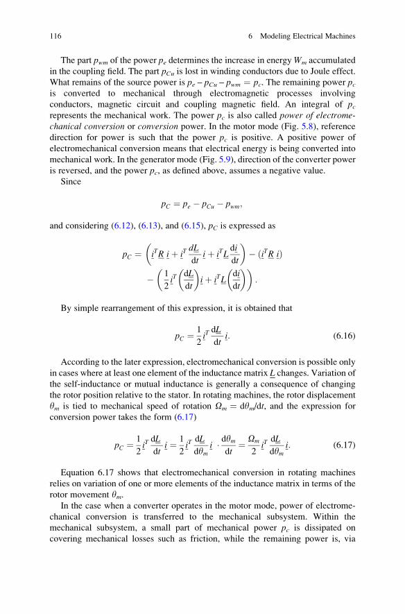
The part pwm of the power pe determines the increase in energyWm accumulated
in the coupling field. The part pCu is lost in winding conductors due to Joule effect.
What remains of the source power is pe – pCu – pwm ¼ pc. The remaining power pcis converted to mechanical through electromagnetic processes involving
conductors, magnetic circuit and coupling magnetic field. An integral of pcrepresents the mechanical work. The power pc is also called power of electrome-chanical conversion or conversion power. In the motor mode (Fig. 5.8), reference
direction for power is such that the power pc is positive. A positive power of
electromechanical conversion means that electrical energy is being converted into
mechanical work. In the generator mode (Fig. 5.9), direction of the converter power
is reversed, and the power pc, as defined above, assumes a negative value.
Since
pC ¼ pe � pCu � pwm;
and considering (6.12), (6.13), and (6.15), pC is expressed as
pC ¼ iTR iþ iTdL
dtiþ iTL
di
dt
� �� ðiTR iÞ
� 1
2iT
dL
dt
� �iþ iTL
di
dt
� �� �:
By simple rearrangement of this expression, it is obtained that
pC ¼ 1
2iTdL
dti: (6.16)
According to the later expression, electromechanical conversion is possible only
in cases where at least one element of the inductance matrix L changes. Variation of
the self-inductance or mutual inductance is generally a consequence of changing
the rotor position relative to the stator. In rotating machines, the rotor displacement
ym is tied to mechanical speed of rotation Om ¼ dym/dt, and the expression for
conversion power takes the form (6.17)
pC ¼ 1
2iTdL
dti ¼ 1
2iT
dL
dymi � dym
dt¼ Om
2iT
dL
dymi: (6.17)
Equation 6.17 shows that electromechanical conversion in rotating machines
relies on variation of one or more elements of the inductance matrix in terms of the
rotor movement ym.In the case when a converter operates in the motor mode, power of electrome-
chanical conversion is transferred to the mechanical subsystem. Within the
mechanical subsystem, a small part of mechanical power pc is dissipated on
covering mechanical losses such as friction, while the remaining power is, via
116 6 Modeling Electrical Machines
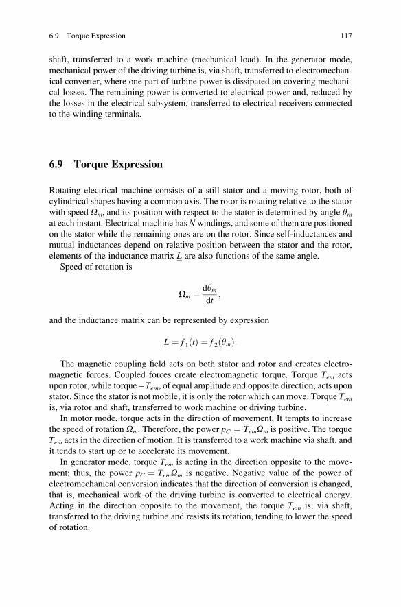
shaft, transferred to a work machine (mechanical load). In the generator mode,
mechanical power of the driving turbine is, via shaft, transferred to electromechan-
ical converter, where one part of turbine power is dissipated on covering mechani-
cal losses. The remaining power is converted to electrical power and, reduced by
the losses in the electrical subsystem, transferred to electrical receivers connected
to the winding terminals.
6.9 Torque Expression
Rotating electrical machine consists of a still stator and a moving rotor, both of
cylindrical shapes having a common axis. The rotor is rotating relative to the stator
with speed Om, and its position with respect to the stator is determined by angle ymat each instant. Electrical machine has Nwindings, and some of them are positioned
on the stator while the remaining ones are on the rotor. Since self-inductances and
mutual inductances depend on relative position between the stator and the rotor,
elements of the inductance matrix L are also functions of the same angle.
Speed of rotation is
Om ¼ dymdt
;
and the inductance matrix can be represented by expression
L ¼ f 1ðtÞ ¼ f 2ðymÞ:
The magnetic coupling field acts on both stator and rotor and creates electro-
magnetic forces. Coupled forces create electromagnetic torque. Torque Tem acts
upon rotor, while torque – Tem, of equal amplitude and opposite direction, acts upon
stator. Since the stator is not mobile, it is only the rotor which can move. Torque Temis, via rotor and shaft, transferred to work machine or driving turbine.
In motor mode, torque acts in the direction of movement. It tempts to increase
the speed of rotation Om. Therefore, the power pC ¼ TemOm is positive. The torque
Tem acts in the direction of motion. It is transferred to a work machine via shaft, and
it tends to start up or to accelerate its movement.
In generator mode, torque Tem is acting in the direction opposite to the move-
ment; thus, the power pC ¼ TemOm is negative. Negative value of the power of
electromechanical conversion indicates that the direction of conversion is changed,
that is, mechanical work of the driving turbine is converted to electrical energy.
Acting in the direction opposite to the movement, the torque Tem is, via shaft,
transferred to the driving turbine and resists its rotation, tending to lower the speed
of rotation.
6.9 Torque Expression 117
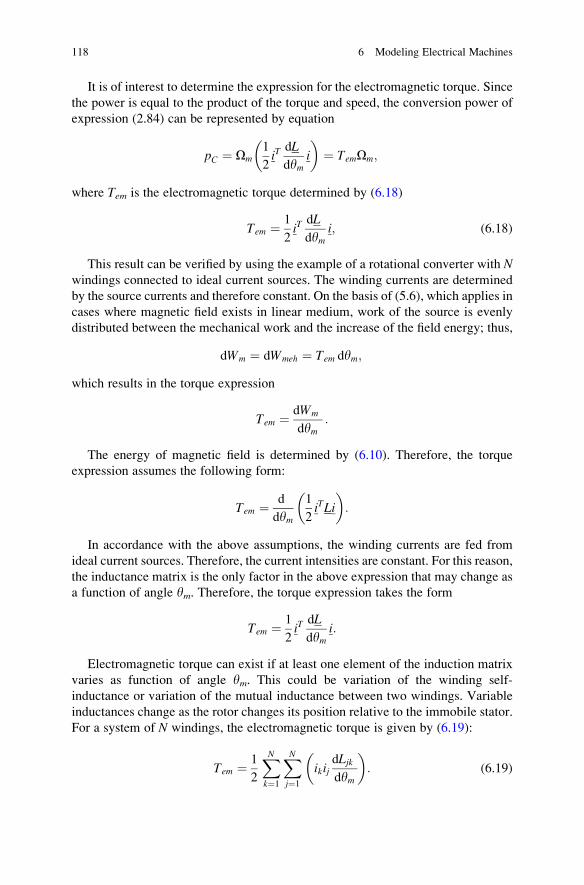
It is of interest to determine the expression for the electromagnetic torque. Since
the power is equal to the product of the torque and speed, the conversion power of
expression (2.84) can be represented by equation
pC ¼ Om1
2iT
dL
dymi
� �¼ TemOm;
where Tem is the electromagnetic torque determined by (6.18)
Tem ¼ 1
2iT
dL
dymi; (6.18)
This result can be verified by using the example of a rotational converter with Nwindings connected to ideal current sources. The winding currents are determined
by the source currents and therefore constant. On the basis of (5.6), which applies in
cases where magnetic field exists in linear medium, work of the source is evenly
distributed between the mechanical work and the increase of the field energy; thus,
dWm ¼ dWmeh ¼ Tem dym;
which results in the torque expression
Tem ¼ dWm
dym:
The energy of magnetic field is determined by (6.10). Therefore, the torque
expression assumes the following form:
Tem ¼ d
dym
1
2iTLi
� �:
In accordance with the above assumptions, the winding currents are fed from
ideal current sources. Therefore, the current intensities are constant. For this reason,
the inductance matrix is the only factor in the above expression that may change as
a function of angle ym. Therefore, the torque expression takes the form
Tem ¼ 1
2iT
dL
dymi:
Electromagnetic torque can exist if at least one element of the induction matrix
varies as function of angle ym. This could be variation of the winding self-
inductance or variation of the mutual inductance between two windings. Variable
inductances change as the rotor changes its position relative to the immobile stator.
For a system of N windings, the electromagnetic torque is given by (6.19):
Tem ¼ 1
2
XNk¼1
XNj¼1
ikijdLjkdym
� �: (6.19)
118 6 Modeling Electrical Machines
Question (6.3): Determine the course of change of the mutual inductance between
two windings, one of them being on the stator and the other on the rotor.
Answer (6.3): Since the rotor revolves, angle ym between the stator and rotor
reference axes varies. Without the lack of generality, it can be assumed that the case
ym ¼ 0 corresponds to the rotor position where the magnetic axes of the two
windings are collinear. In such case, the lines of the magnetic field created by the
stator winding are perpendicular to the surface delineated by the turns of the rotor
winding. The part of the stator flux passing through rotor winding is at a maximum.
Mutual inductance between the two windings is the highest for ym ¼ 0. When the
rotor moves, angle between the field lines and the rotor surface is no longer p/2 buttakes value of p/2�ym. Since the flux is determined by the sine of this angle,
variation of the mutual inductance is determined by function cos ym. Therefore,LSR ¼ Lm cos ym.
Question (6.4): Give an example of a cylindrical machine with one of the stator
windings having the self-inductance that varies with the rotor position.
Answer (6.4): Self-inductance of stator winding depends on the number of turns
and magnetic resistance. Resistance of the magnetic circuit consists of the resistance
of the iron core of the stator, resistance of the magnetic circuit of the rotor, and
magnetic resistance of the air gap, where flux from the stator magnetic circuit passes
to the rotor magnetic circuit and vice versa. Magnetic circuit of the rotor is mainly
cylindrical, and has a circular cross section. By removing some iron on the rotor
sides, the cross section becomes elongated and resembles an ellipse. The elliptical
rotor and cylindrical stator produce a variable air gap. Therefore, the flux extending
along the larger rotor diameter will encounter magnetic resistancemuch smaller than
the flux oriented along the shorter diameter of the elliptical rotor. For this reason, the
stator fluxmeets a variablemagnetic resistance as the rotor revolves. In turn, the self-
inductance LS ¼ NS2/Rm is variable as well.
6.10 Mechanical Subsystem
Moving parts of a rotating electrical machine are magnetic and current circuits of
the rotor, shaft, and bearings. Bearings are usually mounted on both shaft ends.
They hold the rotor shaft firm and collinear with the axis of the stator cylinder.
There are electrical machines having special fans built in the rotor for the purpose
of enhancing the air flow and facilitate the cooling (self-cooling machines).In addition, rotor often has built-in sensors for performing measurements of the
speed of rotation, position, and temperature of the rotor. In some cases, rotor may
contain permanent magnets or semiconductor diodes. When modeling mechanical
subsystem of an electrical machine, these details are not taken into account, and the
rotor is modeled as a homogeneous cylinder of known mass and dimensions. Owing
to the action of electromagnetic forces, torque Tem acts upon the rotor. The rotor is
6.10 Mechanical Subsystem 119
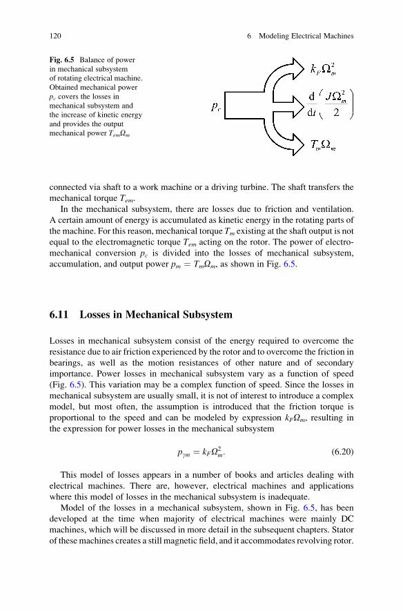
connected via shaft to a work machine or a driving turbine. The shaft transfers the
mechanical torque Tem.In the mechanical subsystem, there are losses due to friction and ventilation.
A certain amount of energy is accumulated as kinetic energy in the rotating parts of
the machine. For this reason, mechanical torque Tm existing at the shaft output is not
equal to the electromagnetic torque Tem acting on the rotor. The power of electro-
mechanical conversion pc is divided into the losses of mechanical subsystem,
accumulation, and output power pm ¼ TmOm, as shown in Fig. 6.5.
6.11 Losses in Mechanical Subsystem
Losses in mechanical subsystem consist of the energy required to overcome the
resistance due to air friction experienced by the rotor and to overcome the friction in
bearings, as well as the motion resistances of other nature and of secondary
importance. Power losses in mechanical subsystem vary as a function of speed
(Fig. 6.5). This variation may be a complex function of speed. Since the losses in
mechanical subsystem are usually small, it is not of interest to introduce a complex
model, but most often, the assumption is introduced that the friction torque is
proportional to the speed and can be modeled by expression kFOm, resulting in
the expression for power losses in the mechanical subsystem
pgm ¼ kFO2m: (6.20)
This model of losses appears in a number of books and articles dealing with
electrical machines. There are, however, electrical machines and applications
where this model of losses in the mechanical subsystem is inadequate.
Model of the losses in a mechanical subsystem, shown in Fig. 6.5, has been
developed at the time when majority of electrical machines were mainly DC
machines, which will be discussed in more detail in the subsequent chapters. Stator
of thesemachines creates a still magnetic field, and it accommodates revolving rotor.
Fig. 6.5 Balance of power
in mechanical subsystem
of rotating electrical machine.
Obtained mechanical power
pc covers the losses inmechanical subsystem and
the increase of kinetic energy
and provides the output
mechanical power TemOm
120 6 Modeling Electrical Machines
Variation of magnetic induction in the rotor magnetic circuit is determined by the
speed of rotation Om. Losses due to eddy currents in the rotor magnetic circuit are
pFe ¼ kVO2m:
Dividing the losses pFe by the speed Om, the torque TFe ¼ pFe/Om is obtained
which resists the rotor motion and tends to diminish the speed. This torque is equal to
TFe ¼ pFeOm
¼ kVOm:
The obtained motion resistance TFe corresponds to the model pgm ¼ kFOm2,
often used in the literature.2
In electrical machines operating at speeds above 1,000 rad/s per second, there is
a substantial air resistance. Forces resisting movement through the air are propor-
tional to the square speed; thus, power of losses due to air friction should be
modeled by expression
pgm ¼ kFO3m:
6.12 Kinetic Energy
Accumulation of energy in the rotating masses is dependent on rotor inertia J. Rotorcan be represented as a homogeneous cylinder of uniform specific mass in all its
parts. With radius R and mass m, resulting moment of inertia is J ¼ ½mR2. Kinetic
energy Wk of a rotor with moment of inertia J and speed Om is Wk ¼ ½ JOm2.
In order to increase kinetic energy, it is necessary to supply the power d(Wk)/
dt ¼ JOm dOm/dt. Therefore, increasing the speed of rotation involves adding an
amount of energy into revolving masses, while in order to slow down a speed
of rotation, the energy should be taken away (by supplying a negative power).
2 Losses pFe in the magnetic field of the rotor of DC machines pFe belong to the losses in magnetic
circuit, that is, to iron losses. Nevertheless, the motion resistance torque TFe arises due to losses
pFe. It is of interest to emphasize that in AC machines having permanent magnets, motion
resistance TFe also appears even in cases with no electric current in the windings. Motion
resistance TFe does not belong to mechanical losses, since it is not caused by friction in the
bearings nor friction with the air, but it is a specific electrical friction. There is, therefore, dilemma
whether power pFe should be classified as motion resistance losses or losses in the magnetic field.
If all the losses that oppose to motion and diminish the speed are classified as motion resistance
losses, whether their cause is mechanical friction or not, then losses in the rotor magnetic circuit of
DCmachines should be classified as motion resistance losses as well. Similar dilemma arises in the
classification of the stator iron losses of synchronous machines having permanent magnets in their
rotors.
6.12 Kinetic Energy 121
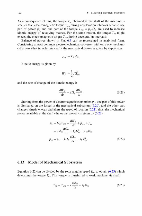
As a consequence of this, the torque Tm obtained at the shaft of the machine is
smaller than electromagnetic torque Tem during acceleration intervals because one
part of power pC and one part of the torque Tem ¼ pC/Om are used to increase
kinetic energy of revolving masses. For the same reason, the torque Tm might
exceed the electromagnetic torque Tem during deceleration intervals.
Balance of power shown in Fig. 6.5 can be represented in analytical form.
Considering a most common electromechanical converter with only one mechani-
cal access (that is, only one shaft), the mechanical power is given by expression
pm ¼ TmOm:
Kinetic energy is given by
Wk ¼ 1
2JO2
m;
and the rate of change of the kinetic energy is
dWk
dt¼ JOm
dOm
dt: (6.21)
Starting from the power of electromagnetic conversion pC, one part of this poweris dissipated on the losses in the mechanical subsystem (6.20), and the other part
changes kinetic energy and alters the speed of rotation (6.21); thus, the mechanical
power available at the shaft (the output power) is given by (6.22):
pc ¼ OmTem ¼ dWk
dtþ pgm þ pm
¼ JOmdOm
dtþ kFO2
m þ TmOm:
pm ¼ pc � JOmdOm
dt� kFO2
m: (6.22)
6.13 Model of Mechanical Subsystem
Equation 6.22 can be divided by the rotor angular speed Om to obtain (6.23) which
determines the torque Tm. This torque is transferred to work machine via shaft.
Tm ¼ Tem � JdOm
dt� kFOm (6.23)
122 6 Modeling Electrical Machines
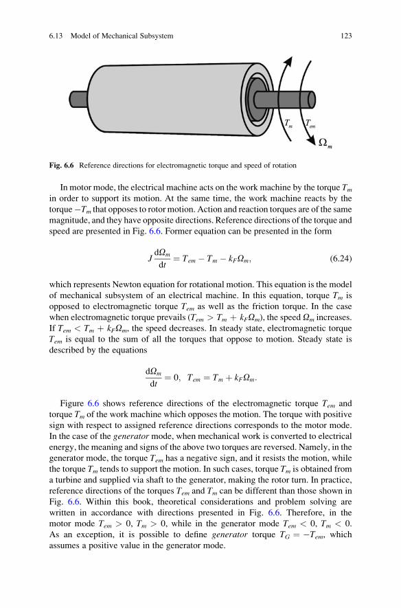
In motor mode, the electrical machine acts on the work machine by the torque Tmin order to support its motion. At the same time, the work machine reacts by the
torque�Tm that opposes to rotor motion. Action and reaction torques are of the same
magnitude, and they have opposite directions. Reference directions of the torque and
speed are presented in Fig. 6.6. Former equation can be presented in the form
JdOm
dt¼ Tem � Tm � kFOm; (6.24)
which represents Newton equation for rotational motion. This equation is the model
of mechanical subsystem of an electrical machine. In this equation, torque Tm is
opposed to electromagnetic torque Tem as well as the friction torque. In the case
when electromagnetic torque prevails (Tem > Tm þ kFOm), the speed Om increases.
If Tem < Tm þ kFOm, the speed decreases. In steady state, electromagnetic torque
Tem is equal to the sum of all the torques that oppose to motion. Steady state is
described by the equations
dOm
dt¼ 0; Tem ¼ Tm þ kFOm:
Figure 6.6 shows reference directions of the electromagnetic torque Tem and
torque Tm of the work machine which opposes the motion. The torque with positive
sign with respect to assigned reference directions corresponds to the motor mode.
In the case of the generator mode, when mechanical work is converted to electrical
energy, the meaning and signs of the above two torques are reversed. Namely, in the
generator mode, the torque Tem has a negative sign, and it resists the motion, while
the torque Tm tends to support the motion. In such cases, torque Tm is obtained from
a turbine and supplied via shaft to the generator, making the rotor turn. In practice,
reference directions of the torques Tem and Tm can be different than those shown in
Fig. 6.6. Within this book, theoretical considerations and problem solving are
written in accordance with directions presented in Fig. 6.6. Therefore, in the
motor mode Tem > 0, Tm > 0, while in the generator mode Tem < 0, Tm < 0.
As an exception, it is possible to define generator torque TG ¼ �Tem, whichassumes a positive value in the generator mode.
Fig. 6.6 Reference directions for electromagnetic torque and speed of rotation
6.13 Model of Mechanical Subsystem 123
The analysis and modeling of the mechanical subsystem apply to electrome-
chanical converters having only one mechanical access. Moving parts in most
electrical machines are rotors with only one degree of freedom. They revolve
around the axis of the cylindrical stator. There is only one shaft attached to the
rotor and positioned along the axis of rotation. The rotor motion is characterized by
unique speed, and it depends on driving torques and motion resistance torques. It is
possible to imagine, design, and produce electromechanical converters whose
mobile parts could move with more than one degree of freedom, involving more
different speeds and a corresponding number of forces and torques acting in
different directions. These converters are not studied in this book.
6.14 Balance of Power in Electromechanical Converters
Diagram presented in Fig. 6.7 shows the power flow in a rotational electromechanical
converter having N windings located on immobile cylindrical stator and on revolving
cylindrical rotor. It is assumed that converter operates with magnetic coupling field.
The relevant powers presented in the figure are explained in the following sequence.
Power at electrical access of the machine, also called input3 power, or electrical
power transferred by the source to the converter is
pe ¼ iTu:
The power lost in the windings due to Joule effect represents losses in the
electrical subsystem. This power is called power of losses in copper, and it is
equal to
pCu ¼ iTR i ¼Xk
Rki2k :
Power which determines the increase of energy of the coupling field is
pwm ¼ dWm
dt¼ 1
2
d
dtiTL i
� �:
Power of losses in the magnetic circuit, also called power of iron losses, amounts
pFe ¼ sHB2f þ sVB2f 2;
and it is neglected in preliminary considerations.
3 For electrical motors, electrical power is supplied to the motor, and it is considered an input.
Mechanical power is obtained on the shaft, and it represents an output. In the case that machine
operates in the generator mode, mechanical power is considered an input, while electrical power is
output.
124 6 Modeling Electrical Machines
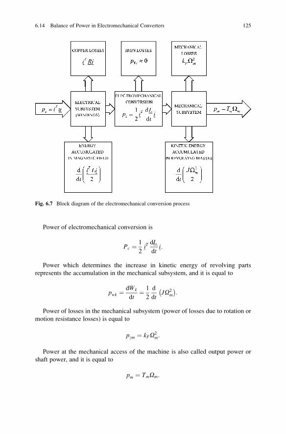
Power of electromechanical conversion is
Pc ¼ 1
2iTdL
dti:
Power which determines the increase in kinetic energy of revolving parts
represents the accumulation in the mechanical subsystem, and it is equal to
pwk ¼dWk
dt¼ 1
2
d
dtJO2
m
� �:
Power of losses in the mechanical subsystem (power of losses due to rotation or
motion resistance losses) is equal to
pgm ¼ kFO2m:
Power at the mechanical access of the machine is also called output power or
shaft power, and it is equal to
pm ¼ TmOm:
Fig. 6.7 Block diagram of the electromechanical conversion process
6.14 Balance of Power in Electromechanical Converters 125
6.15 Equations of Mathematical Model
On the basis of the preceding considerations and introduced approximations, the
mathematical model of an electrical machine with N windings contains:
1. N differential equations expressing the voltage balance (6.7)
2. Inductance matrix which establishes relation between the currents and winding
fluxes (6.9)
3. Expression for electromagnetic torque (6.19)
4. Newton equation of movement (6.24)
Differential equations of the voltage balance are given by expression
u ¼ R � iþ dCd t
: (6.25)
The relation between fluxes and currents is given by the nonstationary induc-
tance matrix
C ¼ LðymÞ � i: (6.26)
The electromagnetic torque is determined by the following equation:
Tem ¼ 1
2iT
dL
dymi ¼ 1
2
XNk¼1
XNj¼1
ikijdLjkdym
� �: (6.27)
According to (6.24), transient phenomena in the mechanical subsystem are
determined by Newton differential equation of motion. The change of the speed
of rotation is determined by expression
JdOm
dt¼ Tem � Tm � kFOm: (6.28)
The four above expressions define general model of a rotational electromechan-
ical converter based on the magnetic coupling field. The model is derived including
the four previously mentioned approximations. Among the approximations are the
assumptions that ferromagnetic materials are linear and that iron losses are
negligible.
The inductance matrix is a nonstationary matrix. In general, elements of the
matrix may be functions of the angle, time, as well as of the flux and current, which
could change the self-inductances and mutual inductances due to nonlinearities in
ferromagnetic materials and due to magnetic saturation. Within the following
considerations, it is considered that the ferromagnetic material is linear and that
126 6 Modeling Electrical Machines
the inductance matrix and its elements are dependent only on the angle ym. Thisapproximation is justified in the majority of cases and will not present an obstacle
in understanding the operation of electrical machines and deriving their
characteristics.
It should be noted in 6.27 that the electromechanical conversion can be accom-
plished only in cases where at least one element of the inductance matrix changes
with the angle ym, either self-inductance of a winding or mutual inductance between
two windings.
In cases where an electrical machine has N windings, expression (6.25) contains
N differential equations of voltage balance, expression (6.26) gives relation
between the winding currents and corresponding fluxes, expression (6.27) gives
electromagnetic torque, and expression (6.28) is Newton differential equation
defining the speed change. Therefore, the model contains N þ 1 differential
equations and the same number of state variables.
6.15 Equations of Mathematical Model 127
Chapter 7
Single-Fed and Double-Fed Converters
In this chapter, examples of single-fed and double electromechanical converters are
analyzed and explained. In both cases, the torque changes are analyzed in cases
where the windings have DC currents and AC currents of adjustable frequency.
Revolving magnetic field created by AC currents in the windings is introduced and
explained. Using the previous considerations, some basic operating principles are
given for DC current machines, induction machines, and synchronous machines.
Electrical machines where one or more self-inductances Lkk vary as a function ofangle ym are usually called single-side supplied converters or single-fed machines.It is shown later that these machines may operate and perform electromechanical
conversion in conditions where only the stator windings are fed from electrical
source. It is also possible to envisage a single-fed electrical machine where only
rotor windings are connected to the source, but this is rarely the case. There exist
single-fed electrical machines having windings on the stator only, while the rotor
contains no windings and has magnetic circuit with magnetic resistance which
depends on the flux direction.
Machines where one or more mutual inductances Lij change with angle ymare called double-side supplied converters or double-fed machines. They have
windings on both stator and rotor. Exception to this rule is synchronous machines
with permanent magnets on the rotor and DC machines with permanent magnets
on the stator, which will be considered later. The effect of permanent magnets on
building the flux is equivalent to effects of windings with direct current mounted
instead of magnets. Therefore, electrical machines with stator windings fed from
electrical source and with permanent magnet on the rotor are classified as double-
fed machines. The same holds for permanent magnet DC machines.
In most cases, the windings of double-fed machine are fed from two different
electrical sources; thus, there are electrical sources for the stator and the rotor. This
two-sided power supply is the reason to call this type of machines double-fedmachines.
S.N. Vukosavic, Electrical Machines, Power Electronics and Power Systems,
DOI 10.1007/978-1-4614-0400-2_7, # Springer Science+Business Media New York 2013
129
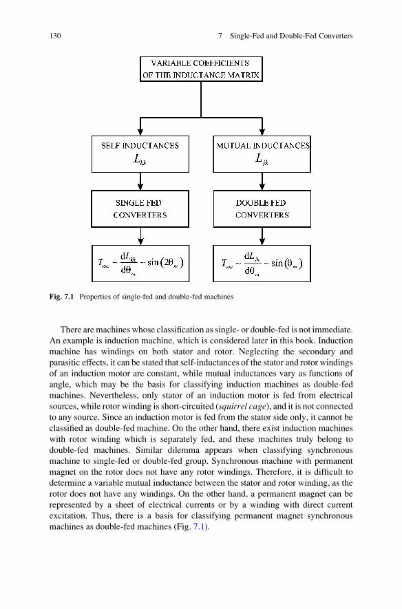
There are machines whose classification as single- or double-fed is not immediate.
An example is induction machine, which is considered later in this book. Induction
machine has windings on both stator and rotor. Neglecting the secondary and
parasitic effects, it can be stated that self-inductances of the stator and rotor windings
of an induction motor are constant, while mutual inductances vary as functions of
angle, which may be the basis for classifying induction machines as double-fed
machines. Nevertheless, only stator of an induction motor is fed from electrical
sources, while rotor winding is short-circuited (squirrel cage), and it is not connectedto any source. Since an induction motor is fed from the stator side only, it cannot be
classified as double-fed machine. On the other hand, there exist induction machines
with rotor winding which is separately fed, and these machines truly belong to
double-fed machines. Similar dilemma appears when classifying synchronous
machine to single-fed or double-fed group. Synchronous machine with permanent
magnet on the rotor does not have any rotor windings. Therefore, it is difficult to
determine a variable mutual inductance between the stator and rotor winding, as the
rotor does not have any windings. On the other hand, a permanent magnet can be
represented by a sheet of electrical currents or by a winding with direct current
excitation. Thus, there is a basis for classifying permanent magnet synchronous
machines as double-fed machines (Fig. 7.1).
Fig. 7.1 Properties of single-fed and double-fed machines
130 7 Single-Fed and Double-Fed Converters
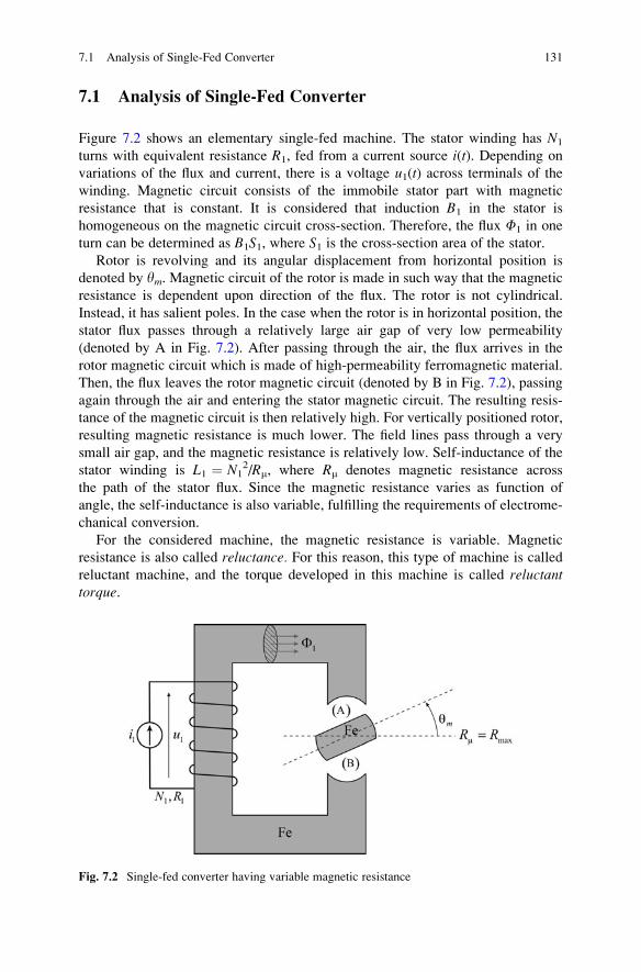
7.1 Analysis of Single-Fed Converter
Figure 7.2 shows an elementary single-fed machine. The stator winding has N1
turns with equivalent resistance R1, fed from a current source i(t). Depending on
variations of the flux and current, there is a voltage u1(t) across terminals of the
winding. Magnetic circuit consists of the immobile stator part with magnetic
resistance that is constant. It is considered that induction B1 in the stator is
homogeneous on the magnetic circuit cross-section. Therefore, the flux F1 in one
turn can be determined as B1S1, where S1 is the cross-section area of the stator.
Rotor is revolving and its angular displacement from horizontal position is
denoted by ym. Magnetic circuit of the rotor is made in such way that the magnetic
resistance is dependent upon direction of the flux. The rotor is not cylindrical.
Instead, it has salient poles. In the case when the rotor is in horizontal position, the
stator flux passes through a relatively large air gap of very low permeability
(denoted by A in Fig. 7.2). After passing through the air, the flux arrives in the
rotor magnetic circuit which is made of high-permeability ferromagnetic material.
Then, the flux leaves the rotor magnetic circuit (denoted by B in Fig. 7.2), passing
again through the air and entering the stator magnetic circuit. The resulting resis-
tance of the magnetic circuit is then relatively high. For vertically positioned rotor,
resulting magnetic resistance is much lower. The field lines pass through a very
small air gap, and the magnetic resistance is relatively low. Self-inductance of the
stator winding is L1 ¼ N12/Rm, where Rm denotes magnetic resistance across
the path of the stator flux. Since the magnetic resistance varies as function of
angle, the self-inductance is also variable, fulfilling the requirements of electrome-
chanical conversion.
For the considered machine, the magnetic resistance is variable. Magnetic
resistance is also called reluctance. For this reason, this type of machine is called
reluctant machine, and the torque developed in this machine is called reluctanttorque.
Fig. 7.2 Single-fed converter having variable magnetic resistance
7.1 Analysis of Single-Fed Converter 131
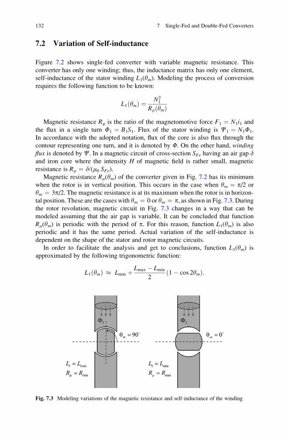
7.2 Variation of Self-inductance
Figure 7.2 shows single-fed converter with variable magnetic resistance. This
converter has only one winding; thus, the inductance matrix has only one element,
self-inductance of the stator winding L1(ym). Modeling the process of conversion
requires the following function to be known:
L1 ymð Þ ¼ N21
Rm ymð ÞMagnetic resistance Rm is the ratio of the magnetomotive force F1 ¼ N1i1 and
the flux in a single turn F1 ¼ B1S1. Flux of the stator winding is C1 ¼ N1F1.
In accordance with the adopted notation, flux of the core is also flux through the
contour representing one turn, and it is denoted by F. On the other hand, windingflux is denoted by C. In a magnetic circuit of cross-section SFe having an air gap dand iron core where the intensity H of magnetic field is rather small, magnetic
resistance is Rm ¼ d/(m0 SFe).Magnetic resistance Rm(ym) of the converter given in Fig. 7.2 has its minimum
when the rotor is in vertical position. This occurs in the case when ym ¼ p/2 or
ym ¼ 3p/2. The magnetic resistance is at its maximum when the rotor is in horizon-
tal position. These are the cases with ym ¼ 0 or ym ¼ p, as shown in Fig. 7.3. Duringthe rotor revolution, magnetic circuit in Fig. 7.3 changes in a way that can be
modeled assuming that the air gap is variable. It can be concluded that function
Rm(ym) is periodic with the period of p. For this reason, function L1(ym) is also
periodic and it has the same period. Actual variation of the self-inductance is
dependent on the shape of the stator and rotor magnetic circuits.
In order to facilitate the analysis and get to conclusions, function L1(ym) is
approximated by the following trigonometric function:
L1 ymð Þ � Lmin þ Lmax � Lmin
21� cos 2ymð Þ:
Fig. 7.3 Modeling variations of the magnetic resistance and self-inductance of the winding
132 7 Single-Fed and Double-Fed Converters
which satisfies conditions L1(p/2) ¼ Lmax, L1(3p/2) ¼ Lmax, L1(0) ¼ Lmin, and
L1(p) ¼ Lmin. Therefore, during one turn of the rotor, the inductance has two
minima and two maxima. Function L1(ym) can be represented in the form given
by (7.1):
L1ðymÞ ¼ 1
2ðLmin þ LmaxÞ � 1
2ðLmax � LminÞ cos 2ym: (7.1)
7.3 The Expressions for Power and Torque
It is of interest to determine the electromagnetic torque and power of electrome-
chanical conversion of the single-fed converter presented in Fig. 7.2. In the case
when the stator winding is connected to a current source i1(t), the energy
accumulated in the magnetic coupling field is
Wm ¼ 1
2L1ðymÞ � i21:
Since the winding is connected to the current source, the torque can be deter-
mined as the first derivative of the field energy Wm. By using expression (7.1) for
self-inductance L1(ym), the electromagnetic torque is determined by (7.2):
Tem ¼ dWm
dym¼ 1
2i21dL1dym
¼ 1
2i21ðLmax � LminÞ sin 2ym: (7.2)
The obtained torque is proportional to the difference between the maximum and
minimum inductance, current squared, and sine of doubled angle. Since the flux is
proportional to the current, the electromagnetic torque can be also expressed as a
function of the flux squared,
Tem � i2 � F2: (7.3)
The highest value of the electromagnetic torque is obtained for ym ¼ p/4 and
ym ¼ 5p/4, while in positions ym ¼ p/2, ym ¼ 3p/2, ym ¼ 0, and ym ¼ p, thetorque is equal to zero. In the case when stator current is constant, i1(t) ¼ I1, andthe rotor is moving at a constant speed Om, the torque is proportional to function sin
(2Omt + y0) and its average value is equal to zero. For this reason, the average valueof power of electromagnetic conversion is also equal to zero. In other words, the
converter shown in Fig. 7.2 with constant (DC) current in the winding cannot
perform electromechanical conversion since the average torque and power in one
revolution are both equal to zero.
7.3 The Expressions for Power and Torque 133
The torque and power with an average values different than zero can be obtained
where the winding has an alternating current. For current with angular frequency
os, with amplitude Im, and with initial phase �’, squared instantaneous current
value is
i21 ¼ Imax sinðost� ’Þ½ �2 ¼ I2max
2ð1� cosð2ost� 2’ÞÞ:
On the basis of (7.2), the electromagnetic torque of single-fed converter with
alternating current in its winding is
Tem ¼ I2max
41� cos 2ost� 2’ð Þð Þ � ðLmax � LminÞ sin 2ym:
By introducing constant
Km ¼ I2max
8ðLmax � LminÞ;
expression for the electromagnetic torque obtains the following form:
Tem ¼ 2Km sin 2ym � 2Km cos 2ost� 2’ð Þ sin 2ym¼ 2Km sin 2ym � Km sin 2ym þ 2ost� 2’ð Þ� Km sin 2ym � 2ostþ 2’ð Þ:
Since the rotor revolves at a constant speed, position of the rotor is determined
by expression ym(t) ¼ Omt + y0. Taking into account that ym(0) ¼ y0 ¼ 0, position
of the rotor takes the value ym(t) ¼ Omt; thus, the torque is equal to
Tem ¼ 2Km sin 2Omt� Km sin 2Omtþ 2ost� 2’ð Þ� Km sin 2Omt� 2ostþ 2’ð Þ : (7.4)
The first member in the above expression is a harmonic function with average
value equal to zero. The same conclusion applies to the second member, except in
cases where Om + os ¼ 0. The third member has a nonzero average value if
Om ¼ os. Therefore, a nonzero average value of the torque can be obtained if the
angular frequency of stator current is equal to the angular frequency of rotation.
The torque is also dependent on the initial phase of the current. By selecting the
corresponding phase, one may accomplish either positive or negative average
torque. In the case when Om ¼ os and ’ ¼ 3p/4, average value of the electromag-
netic torque is
Tav ¼ I2max
8ðLmax � LminÞ:
134 7 Single-Fed and Double-Fed Converters
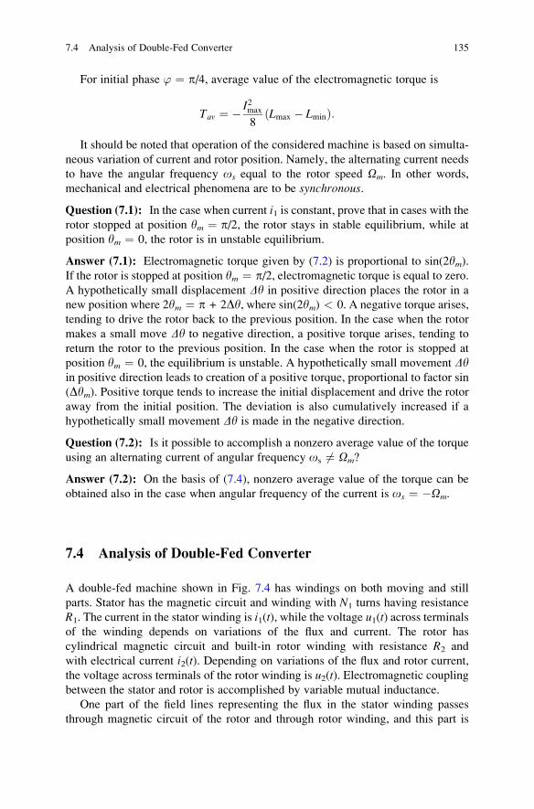
For initial phase ’ ¼ p/4, average value of the electromagnetic torque is
Tav ¼ � I2max
8ðLmax � LminÞ:
It should be noted that operation of the considered machine is based on simulta-
neous variation of current and rotor position. Namely, the alternating current needs
to have the angular frequency os equal to the rotor speed Om. In other words,
mechanical and electrical phenomena are to be synchronous.
Question (7.1): In the case when current i1 is constant, prove that in cases with therotor stopped at position ym ¼ p/2, the rotor stays in stable equilibrium, while at
position ym ¼ 0, the rotor is in unstable equilibrium.
Answer (7.1): Electromagnetic torque given by (7.2) is proportional to sin(2ym).If the rotor is stopped at position ym ¼ p/2, electromagnetic torque is equal to zero.
A hypothetically small displacement Dy in positive direction places the rotor in a
new position where 2ym ¼ p + 2Dy, where sin(2ym) < 0. A negative torque arises,
tending to drive the rotor back to the previous position. In the case when the rotor
makes a small move Dy to negative direction, a positive torque arises, tending to
return the rotor to the previous position. In the case when the rotor is stopped at
position ym ¼ 0, the equilibrium is unstable. A hypothetically small movement Dyin positive direction leads to creation of a positive torque, proportional to factor sin
(Dym). Positive torque tends to increase the initial displacement and drive the rotor
away from the initial position. The deviation is also cumulatively increased if a
hypothetically small movement Dy is made in the negative direction.
Question (7.2): Is it possible to accomplish a nonzero average value of the torque
using an alternating current of angular frequency os 6¼ Om?
Answer (7.2): On the basis of (7.4), nonzero average value of the torque can be
obtained also in the case when angular frequency of the current is os ¼ �Om.
7.4 Analysis of Double-Fed Converter
A double-fed machine shown in Fig. 7.4 has windings on both moving and still
parts. Stator has the magnetic circuit and winding with N1 turns having resistance
R1. The current in the stator winding is i1(t), while the voltage u1(t) across terminals
of the winding depends on variations of the flux and current. The rotor has
cylindrical magnetic circuit and built-in rotor winding with resistance R2 and
with electrical current i2(t). Depending on variations of the flux and rotor current,
the voltage across terminals of the rotor winding is u2(t). Electromagnetic coupling
between the stator and rotor is accomplished by variable mutual inductance.
One part of the field lines representing the flux in the stator winding passes
through magnetic circuit of the rotor and through rotor winding, and this part is
7.4 Analysis of Double-Fed Converter 135
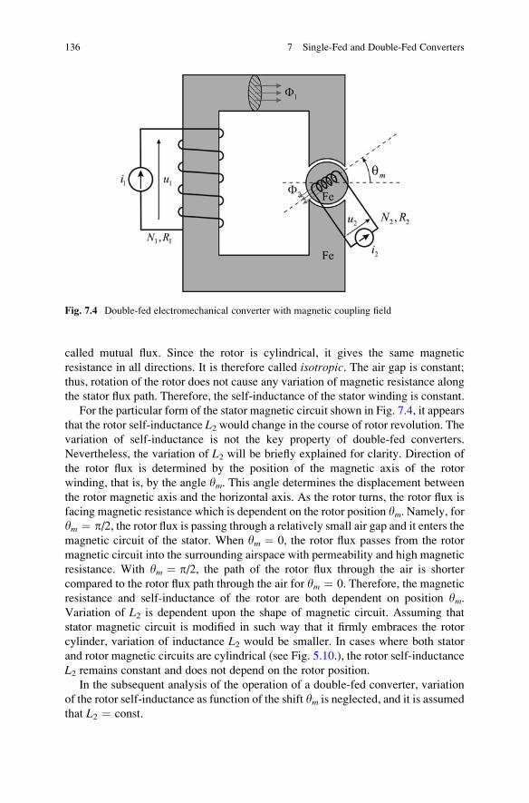
called mutual flux. Since the rotor is cylindrical, it gives the same magnetic
resistance in all directions. It is therefore called isotropic. The air gap is constant;
thus, rotation of the rotor does not cause any variation of magnetic resistance along
the stator flux path. Therefore, the self-inductance of the stator winding is constant.
For the particular form of the stator magnetic circuit shown in Fig. 7.4, it appears
that the rotor self-inductance L2 would change in the course of rotor revolution. Thevariation of self-inductance is not the key property of double-fed converters.
Nevertheless, the variation of L2 will be briefly explained for clarity. Direction of
the rotor flux is determined by the position of the magnetic axis of the rotor
winding, that is, by the angle ym. This angle determines the displacement between
the rotor magnetic axis and the horizontal axis. As the rotor turns, the rotor flux is
facing magnetic resistance which is dependent on the rotor position ym. Namely, for
ym ¼ p/2, the rotor flux is passing through a relatively small air gap and it enters the
magnetic circuit of the stator. When ym ¼ 0, the rotor flux passes from the rotor
magnetic circuit into the surrounding airspace with permeability and high magnetic
resistance. With ym ¼ p/2, the path of the rotor flux through the air is shorter
compared to the rotor flux path through the air for ym ¼ 0. Therefore, the magnetic
resistance and self-inductance of the rotor are both dependent on position ym.Variation of L2 is dependent upon the shape of magnetic circuit. Assuming that
stator magnetic circuit is modified in such way that it firmly embraces the rotor
cylinder, variation of inductance L2 would be smaller. In cases where both stator
and rotor magnetic circuits are cylindrical (see Fig. 5.10.), the rotor self-inductance
L2 remains constant and does not depend on the rotor position.
In the subsequent analysis of the operation of a double-fed converter, variation
of the rotor self-inductance as function of the shift ym is neglected, and it is assumed
that L2 ¼ const.
Fig. 7.4 Double-fed electromechanical converter with magnetic coupling field
136 7 Single-Fed and Double-Fed Converters
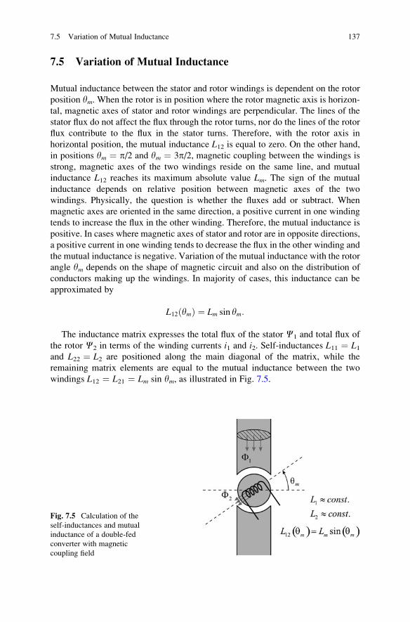
7.5 Variation of Mutual Inductance
Mutual inductance between the stator and rotor windings is dependent on the rotor
position ym. When the rotor is in position where the rotor magnetic axis is horizon-
tal, magnetic axes of stator and rotor windings are perpendicular. The lines of the
stator flux do not affect the flux through the rotor turns, nor do the lines of the rotor
flux contribute to the flux in the stator turns. Therefore, with the rotor axis in
horizontal position, the mutual inductance L12 is equal to zero. On the other hand,
in positions ym ¼ p/2 and ym ¼ 3p/2, magnetic coupling between the windings is
strong, magnetic axes of the two windings reside on the same line, and mutual
inductance L12 reaches its maximum absolute value Lm. The sign of the mutual
inductance depends on relative position between magnetic axes of the two
windings. Physically, the question is whether the fluxes add or subtract. When
magnetic axes are oriented in the same direction, a positive current in one winding
tends to increase the flux in the other winding. Therefore, the mutual inductance is
positive. In cases where magnetic axes of stator and rotor are in opposite directions,
a positive current in one winding tends to decrease the flux in the other winding and
the mutual inductance is negative. Variation of the mutual inductance with the rotor
angle ym depends on the shape of magnetic circuit and also on the distribution of
conductors making up the windings. In majority of cases, this inductance can be
approximated by
L12ðymÞ ¼ Lm sin ym:
The inductance matrix expresses the total flux of the stator C1 and total flux of
the rotor C2 in terms of the winding currents i1 and i2. Self-inductances L11 ¼ L1and L22 ¼ L2 are positioned along the main diagonal of the matrix, while the
remaining matrix elements are equal to the mutual inductance between the two
windings L12 ¼ L21 ¼ Lm sin ym, as illustrated in Fig. 7.5.
Fig. 7.5 Calculation of the
self-inductances and mutual
inductance of a double-fed
converter with magnetic
coupling field
7.5 Variation of Mutual Inductance 137
C ¼ C1
C2
" #¼ L11
L21
"L12
L22
#i1
i2
" #¼ L1
L12
"L12
L2
#i1
i2
" #¼ L i: (7.5)
The energy of magnetic field can be expressed as function of currents and
elements in the inductance matrix. Expression for the energy can be given in the
form of a sum, in the matrix form, or as a scalar expression
Wm ¼ 1
2
X2j¼1
X2k¼1
Ljkijik
¼ 1
2L1i
21 þ
1
2L2i
22 þ L12i1i2 ¼ 1
2iTL i: (7.6)
7.6 Torque Expression
Since the mutual inductance is variable and it changes with the rotor position, one
of the three members in the expression for the field energy (7.6) varies with angle
ym in the following manner:
L12i1i2 ¼ i1i2 Lm sin ym: (7.7)
The electromagnetic torque can be determined as the first derivative of the field
energy Wm. Expression for the electromagnetic torque, given by (7.8), shows that
the torque is proportional to the product of the currents in the stator and rotor
windings and that it is dependent on the mutual inductance Lm as the angle ym.Namely, it changes with cosym.
Tem ¼ dWm
dym¼ d
dym
1
2L1i
21 þ
1
2L2i
22 þ L12i1i2
� �¼ i1i2Lm cos ym: (7.8)
The electromagnetic torque of a double-fed machine can be expressed as a
product of two currents but can also be written as a product of two fluxes. In order
to prove this statement, it is necessary to express the currents in terms of the fluxes,
which is accomplished by inverting the inductance matrix,
C ¼ L i ) i ¼ L�1 C ;
resulting in the expressions for the currents
i1 ¼ L2L1L2 � L212
C1 � L12L1L2 � L212
C2;
i2 ¼ �L12L1L2 � L212
C1 þ L1L1L2 � L212
C2:
138 7 Single-Fed and Double-Fed Converters
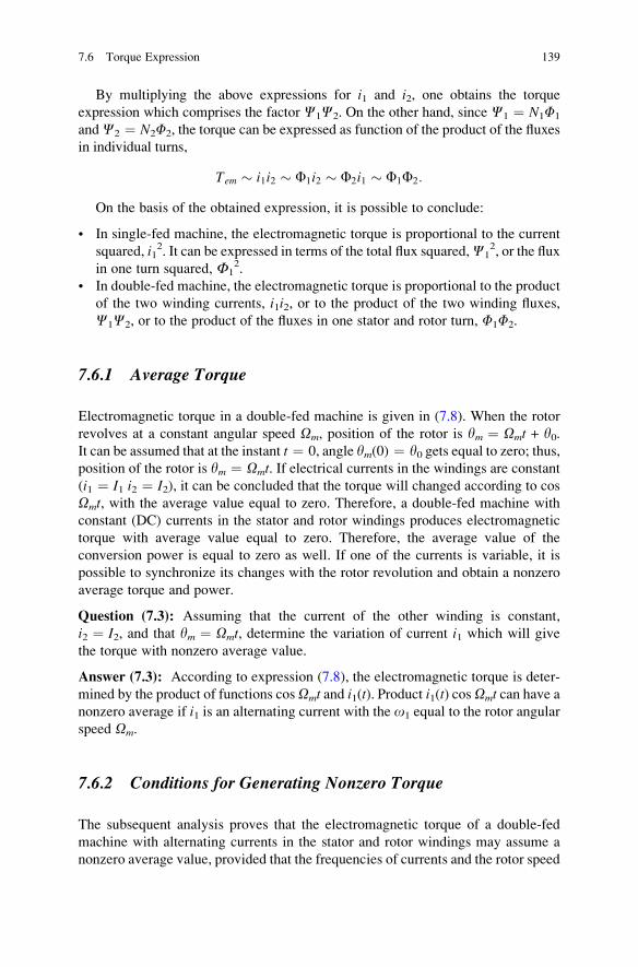
By multiplying the above expressions for i1 and i2, one obtains the torque
expression which comprises the factor C1C2. On the other hand, since C1 ¼ N1F1
andC2 ¼ N2F2, the torque can be expressed as function of the product of the fluxes
in individual turns,
Tem � i1i2 � F1i2 � F2i1 � F1F2:
On the basis of the obtained expression, it is possible to conclude:
• In single-fed machine, the electromagnetic torque is proportional to the current
squared, i12. It can be expressed in terms of the total flux squared,C1
2, or the flux
in one turn squared, Ф12.
• In double-fed machine, the electromagnetic torque is proportional to the product
of the two winding currents, i1i2, or to the product of the two winding fluxes,
C1C2, or to the product of the fluxes in one stator and rotor turn, F1F2.
7.6.1 Average Torque
Electromagnetic torque in a double-fed machine is given in (7.8). When the rotor
revolves at a constant angular speed Om, position of the rotor is ym ¼ Omt + y0.It can be assumed that at the instant t ¼ 0, angle ym(0) ¼ y0 gets equal to zero; thus,position of the rotor is ym ¼ Omt. If electrical currents in the windings are constant(i1 ¼ I1 i2 ¼ I2), it can be concluded that the torque will changed according to cos
Omt, with the average value equal to zero. Therefore, a double-fed machine with
constant (DC) currents in the stator and rotor windings produces electromagnetic
torque with average value equal to zero. Therefore, the average value of the
conversion power is equal to zero as well. If one of the currents is variable, it is
possible to synchronize its changes with the rotor revolution and obtain a nonzero
average torque and power.
Question (7.3): Assuming that the current of the other winding is constant,
i2 ¼ I2, and that ym ¼ Omt, determine the variation of current i1 which will give
the torque with nonzero average value.
Answer (7.3): According to expression (7.8), the electromagnetic torque is deter-
mined by the product of functions cosOmt and i1(t). Product i1(t) cos Omt can have anonzero average if i1 is an alternating current with the o1 equal to the rotor angular
speed Om.
7.6.2 Conditions for Generating Nonzero Torque
The subsequent analysis proves that the electromagnetic torque of a double-fed
machine with alternating currents in the stator and rotor windings may assume a
nonzero average value, provided that the frequencies of currents and the rotor speed
7.6 Torque Expression 139
meet certain conditions. The currents can be expressed in terms of their amplitude I,angular frequency o, and initial phase, i ¼ I cos(ot�’). When both the stator and
rotor currents have nonzero angular frequencies, they change periodically, as well
as the stator and rotor fluxes. It is also possible to distinguish the case where one of
the currents has its angular frequency equal to zero, o ¼ 0. This actually means
that such current does not change, maintaining the value of i ¼ I cos(’). As a
matter of fact, o ¼ 0 results in a DC current. The currents of the stator and rotor
may have different amplitudes, frequencies, and initial phases. Let the angular
frequency of the stator current be o1, the angular frequency of the rotor current
o2, the relevant amplitudes I1m and I2m, and the initial phases �’1 and �’2.
Instantaneous values of the winding currents are given by (7.9):
i1 ¼ I1m cosðo1t� ’1Þ;i2 ¼ I2m cosðo2t� ’2Þ: (7.9)
By introducing these expressions into (7.8), one obtains the electromagnetic
torque as
Tem ¼ i1i2Lm cos ym¼ I1m cosðo1t� ’1Þ � I2m cosðo2t� ’2Þ � Lm cos ym :
With ym ¼ Omt, the torque Tem is a product of three periodic functions. By
introducing coefficient Kn ¼ LmI1mI2m/4, this equation assumes the form
Tem ¼ Kn cos ðo1t� ’1 þ o2t� ’2 þ OmtÞþ Kn cos ðo1t� ’1 þ o2t� ’2 � OmtÞþ Kn cos ðo1t� ’1 � o2tþ ’2 þ OmtÞþ Kn cosðo1t� ’1 � o2tþ ’2 � OmtÞ: (7.10)
The electromagnetic torque has the amplitude proportional to the mutual induc-
tance and to the product of the amplitudes of thewinding currents (Lm I1m I2m ¼ 4Kn).
Variation of the torque is determined by four cosine functions having different
frequencies. Their frequencies can be expressed byo1 � o2 � Om. For the function
cos(ot�’) to assume a nonzero average value, it is necessary that the angular
frequency o is equal to zero. Hence, for the expression (7.10) to have a nonzero
average value, one of frequencieso1 � o2 � Om has to be equal to zero. Therefore,
conclusion is reached that a nonzero average value of the torque Tem is obtained in
cases where the angular frequencies (o1 ando2) of electrical currents in the windings
and the rotor speed Om meet one out of four conditions given in expression (7.11):
Om ¼ o1 þ o2;
Om ¼ o1 � o2;
Om ¼ �o1 þ o2;
Om ¼ �o1 � o2: (7.11)
140 7 Single-Fed and Double-Fed Converters
7.7 Magnetic Poles
Double-fed electrical machine has magnetic circuit where it is possible to observe
two magnetic poles of the stator and two magnetic poles of the rotor. Position of the
north magnetic pole of the rotor can be determined as a zone where the lines of
magnetic field, created by electrical currents in the rotor windings, come out of the
rotor magnetic circuit and enter the air gap. Similarly, one can define the southmagnetic pole of the rotor, as well as the magnetic poles of the stator. Double-fed
machine under the scope has two stator poles and two rotor poles. Since L12 ¼ Lmsinym, it can be concluded that one cycle of variation of the mutual inductance
corresponds to one full mechanical rotation of the rotor.
In due course, multipole machines will be defined and explained. The matter
concerns electrical machines made to have more than one pair of magnetic poles.
In most cases, the number of poles on the stator is equal to the number of rotor
poles. A four pole machine has two north and two south poles on the stator and the
same number of poles on the rotor. Such machine is said to have p ¼ 2 pairs of
poles. In a four pole double-fed machine, mutual inductance varies as L12 ¼ Lm sin
(pym) ¼ Lm sin(2ym), thus making two cycles during one revolution of the rotor.
A nonzero average value of the torque is obtained in the case when � o1 � o2 �pOm ¼ 0, where Om denotes the mechanical angular frequency of the rotor motion.
In this book, letter o denotes the angular frequencies of voltages and currents,
while letter Om denotes the speed of rotor motion, also called mechanical angular
speed. The former is often referred to as the electrical frequency o, while the lateris called mechanical speed O. Therefrom, mechanical speed Om may have its
electrical counterpart om ¼ pOm.
Later on, revolving vectors are defined representing the spatial distribution of the
magnetic induction B, magnetic field H, but also the voltages and currents in
multiphase winding. The speed of rotation of such vectors in space is also denoted
by letters O.The expressions electrical frequency o and mechanical speed O will be better
defined in the course of presentation, as well as the relation o ¼ pO. For the time
being, it is understood that two-pole machines are considered, resulting in p ¼ 1
and o ¼ O, unless otherwise stated.
7.8 Direct Current and Alternating Current Machines
The analysis of double-fed machines can be used for demonstration of the basic
operating principles of DC machines, induction machines, and synchronous
machines. The latter two are also called AC machines. These machines will be
studied in the remaining part of the book. All three types of machines have windings
on both stator and rotor. Rotation of the rotor changes mutual inductance between
the stator and rotor windings.
7.8 Direct Current and Alternating Current Machines 141
It has been shown that development of electromagnetic torque with nonzero
average value requires the electrical stator frequency o1, electrical rotor frequency
o2, and the rotor speed Om1 to meet the condition o1 � o2 � om ¼ 0.
DCmachines have a DC current in the stator windings (o1 ¼ 0), while in the rotor
windings they have an AC current. The angular frequency of the rotor currents is
determined by the speed of rotation, o2 ¼ pOm2.
Induction machines have alternating currents in stator windings and alternating
currents in rotor windings. According to (7.11), the sum of pOm3 and rotor fre-
quency o2 has to be equal to the stator frequency o1. Therefore, pOm ¼ o1�o2.
The rotor mechanical speed Om lags behind o1/p by o2/p. The rotor frequency
o2 ¼ o1�pOm of induction machines is also called slip frequency, as it defines theslip of the rotor speed behind the value of o1/p, determined by the stator frequency
and called synchronous speed.
Synchronous machines have alternating currents in stator windings, while the rotor
conductors carry DC current. Since o2 ¼ 0, condition (7.11) reduces to o1 ¼ pOm.
Therefore, the rotor speed Om is uniquely determined by the stator electrical fre-
quency, Om ¼ o1/p. Hence, all the two-pole (p ¼ 1) synchronous machines
connected to the three-phase grid with the line frequency of fs ¼ 50 Hz make 50
turns per second, or 50�60 ¼ 3,000 revolutions per minute (rpm). A four pole (p ¼ 2)
synchronous machine supplied by fs ¼ 60 Hz runs at 60�60/p ¼ 1,800 rpm. Hence,
thesemachines run synchronouslywith the supply frequency and therefore their name.
7.9 Torque as a Vector Product
The principles of operation of DC machines, induction, and synchronous machines
as well as the main differences between them are more obvious when the stator and
rotor fluxes are represented by corresponding vectors. Electromagnetic torque can
1 In cases where machine has p pairs of poles, the condition for torque development is o1 � o2
� pOm ¼ 0. Notation Om is angular speed of rotor motion, hence mechanical speed. Angular
frequency om ¼ pOm is electrical representation of the rotor speed. It defines the period Tom ¼ 2
p/om which marks passing of north magnetic poles of the rotor against north magnetic poles of the
stator. With p > 1, this happens more than once per each mechanical revolution. In a machine with
p > 1 pole pairs, angular distance between the two neighboring north poles is OmTom ¼ 2p/p.A four pole machine (p ¼ 2) has two north and two south poles. Two north poles are at angular
distance of OmTom ¼ 2p/2 ¼ p. Therefore, any north magnetic pole of the rotor passes against
stator north pole twice per turn. In a two-pole machine (p ¼ 1), starting from the north magnetic
pole, one should pass angular distance of OmTom ¼ 2p/1 ¼ 2p in order to arrive at the next
north pole, the very same pole from where one started. Namely, a two-pole machine has only one
north magnetic pole and one south magnetic pole.2 In a two-pole DC machine, the number of pole pairs is p ¼ 1. Therefore, o2 ¼ pOm ¼ Om. With
p > 1, the condition reads o2 ¼ om ¼ pOm.3 In a two-pole induction motor, p ¼ 1.
142 7 Single-Fed and Double-Fed Converters
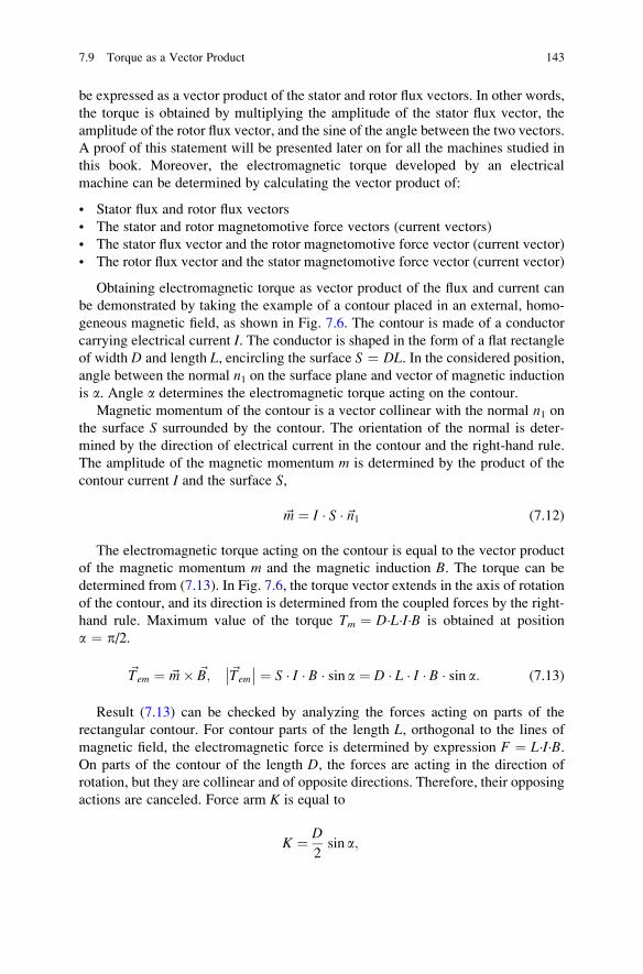
be expressed as a vector product of the stator and rotor flux vectors. In other words,
the torque is obtained by multiplying the amplitude of the stator flux vector, the
amplitude of the rotor flux vector, and the sine of the angle between the two vectors.
A proof of this statement will be presented later on for all the machines studied in
this book. Moreover, the electromagnetic torque developed by an electrical
machine can be determined by calculating the vector product of:
• Stator flux and rotor flux vectors
• The stator and rotor magnetomotive force vectors (current vectors)
• The stator flux vector and the rotor magnetomotive force vector (current vector)
• The rotor flux vector and the stator magnetomotive force vector (current vector)
Obtaining electromagnetic torque as vector product of the flux and current can
be demonstrated by taking the example of a contour placed in an external, homo-
geneous magnetic field, as shown in Fig. 7.6. The contour is made of a conductor
carrying electrical current I. The conductor is shaped in the form of a flat rectangle
of width D and length L, encircling the surface S ¼ DL. In the considered position,angle between the normal n1 on the surface plane and vector of magnetic induction
is a. Angle a determines the electromagnetic torque acting on the contour.
Magnetic momentum of the contour is a vector collinear with the normal n1 onthe surface S surrounded by the contour. The orientation of the normal is deter-
mined by the direction of electrical current in the contour and the right-hand rule.
The amplitude of the magnetic momentum m is determined by the product of the
contour current I and the surface S,
~m ¼ I � S �~n1 (7.12)
The electromagnetic torque acting on the contour is equal to the vector product
of the magnetic momentum m and the magnetic induction B. The torque can be
determined from (7.13). In Fig. 7.6, the torque vector extends in the axis of rotation
of the contour, and its direction is determined from the coupled forces by the right-
hand rule. Maximum value of the torque Tm ¼ D�L�I�B is obtained at position
a ¼ p/2.
~Tem ¼ ~m� ~B; ~Tem
�� �� ¼ S � I � B � sin a ¼ D � L � I � B � sin a: (7.13)
Result (7.13) can be checked by analyzing the forces acting on parts of the
rectangular contour. For contour parts of the length L, orthogonal to the lines of
magnetic field, the electromagnetic force is determined by expression F ¼ L�I�B.On parts of the contour of the length D, the forces are acting in the direction of
rotation, but they are collinear and of opposite directions. Therefore, their opposing
actions are canceled. Force arm K is equal to
K ¼ D
2sin a;
7.9 Torque as a Vector Product 143
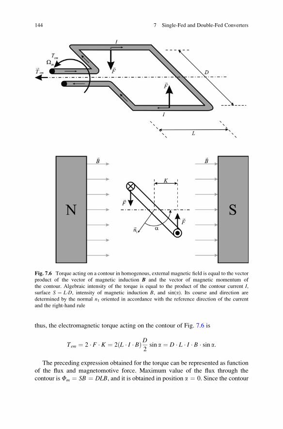
thus, the electromagnetic torque acting on the contour of Fig. 7.6 is
Tem ¼ 2 � F � K ¼ 2 L � I � Bð ÞD2sin a ¼ D � L � I � B � sin a:
The preceding expression obtained for the torque can be represented as function
of the flux and magnetomotive force. Maximum value of the flux through the
contour is Fm ¼ SB ¼ DLB, and it is obtained in position a ¼ 0. Since the contour
Fig. 7.6 Torque acting on a contour in homogenous, external magnetic field is equal to the vector
product of the vector of magnetic induction B and the vector of magnetic momentum of
the contour. Algebraic intensity of the torque is equal to the product of the contour current I,surface S ¼ L�D, intensity of magnetic induction B, and sin(a). Its course and direction are
determined by the normal n1 oriented in accordance with the reference direction of the current
and the right-hand rule
144 7 Single-Fed and Double-Fed Converters
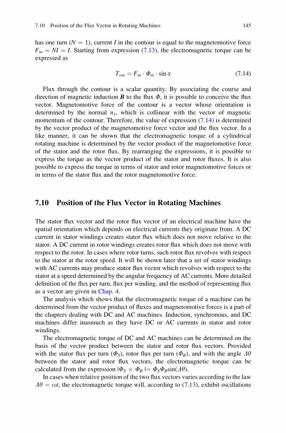
has one turn (N ¼ 1), current I in the contour is equal to the magnetomotive force
Fm ¼ NI ¼ I. Starting from expression (7.13), the electromagnetic torque can be
expressed as
Tem ¼ Fm � Fm � sin a (7.14)
Flux through the contour is a scalar quantity. By associating the course and
direction of magnetic induction B to the flux F, it is possible to conceive the flux
vector. Magnetomotive force of the contour is a vector whose orientation is
determined by the normal n1, which is collinear with the vector of magnetic
momentum of the contour. Therefore, the value of expression (7.14) is determined
by the vector product of the magnetomotive force vector and the flux vector. In a
like manner, it can be shown that the electromagnetic torque of a cylindrical
rotating machine is determined by the vector product of the magnetomotive force
of the stator and the rotor flux. By rearranging the expressions, it is possible to
express the torque as the vector product of the stator and rotor fluxes. It is also
possible to express the torque in terms of stator and rotor magnetomotive forces or
in terms of the stator flux and the rotor magnetomotive force.
7.10 Position of the Flux Vector in Rotating Machines
The stator flux vector and the rotor flux vector of an electrical machine have the
spatial orientation which depends on electrical currents they originate from. A DC
current in stator windings creates stator flux which does not move relative to the
stator. A DC current in rotor windings creates rotor flux which does not move with
respect to the rotor. In cases where rotor turns, such rotor flux revolves with respect
to the stator at the rotor speed. It will be shown later that a set of stator windings
with AC currents may produce stator flux vector which revolves with respect to the
stator at a speed determined by the angular frequency of AC currents. More detailed
definition of the flux per turn, flux per winding, and the method of representing flux
as a vector are given in Chap. 4.
The analysis which shows that the electromagnetic torque of a machine can be
determined from the vector product of fluxes and magnetomotive forces is a part of
the chapters dealing with DC and AC machines. Induction, synchronous, and DC
machines differ inasmuch as they have DC or AC currents in stator and rotor
windings.
The electromagnetic torque of DC and AC machines can be determined on the
basis of the vector product between the stator and rotor flux vectors. Provided
with the stator flux per turn (FS), rotor flux per turn (FR), and with the angle Dybetween the stator and rotor flux vectors, the electromagnetic torque can be
calculated from the expression |FS � FR |¼ FSFRsin(Dy).In cases when relative position of the two flux vectors varies according to the law
Dy ¼ ot, the electromagnetic torque will, according to (7.13), exhibit oscillations
7.10 Position of the Flux Vector in Rotating Machines 145
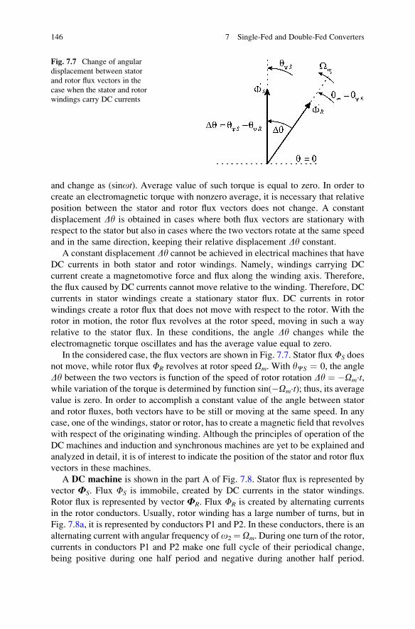
and change as (sinot). Average value of such torque is equal to zero. In order to
create an electromagnetic torque with nonzero average, it is necessary that relative
position between the stator and rotor flux vectors does not change. A constant
displacement Dy is obtained in cases where both flux vectors are stationary with
respect to the stator but also in cases where the two vectors rotate at the same speed
and in the same direction, keeping their relative displacement Dy constant.
A constant displacement Dy cannot be achieved in electrical machines that have
DC currents in both stator and rotor windings. Namely, windings carrying DC
current create a magnetomotive force and flux along the winding axis. Therefore,
the flux caused by DC currents cannot move relative to the winding. Therefore, DC
currents in stator windings create a stationary stator flux. DC currents in rotor
windings create a rotor flux that does not move with respect to the rotor. With the
rotor in motion, the rotor flux revolves at the rotor speed, moving in such a way
relative to the stator flux. In these conditions, the angle Dy changes while the
electromagnetic torque oscillates and has the average value equal to zero.
In the considered case, the flux vectors are shown in Fig. 7.7. Stator flux FS does
not move, while rotor flux FR revolves at rotor speed Om. With yCS ¼ 0, the angle
Dy between the two vectors is function of the speed of rotor rotation Dy ¼ �Om�t,while variation of the torque is determined by function sin(�Om�t); thus, its averagevalue is zero. In order to accomplish a constant value of the angle between stator
and rotor fluxes, both vectors have to be still or moving at the same speed. In any
case, one of the windings, stator or rotor, has to create a magnetic field that revolves
with respect of the originating winding. Although the principles of operation of the
DC machines and induction and synchronous machines are yet to be explained and
analyzed in detail, it is of interest to indicate the position of the stator and rotor flux
vectors in these machines.
A DC machine is shown in the part A of Fig. 7.8. Stator flux is represented by
vector FS. Flux FS is immobile, created by DC currents in the stator windings.
Rotor flux is represented by vector FR. Flux FR is created by alternating currents
in the rotor conductors. Usually, rotor winding has a large number of turns, but in
Fig. 7.8a, it is represented by conductors P1 and P2. In these conductors, there is an
alternating current with angular frequency ofo2¼Om. During one turn of the rotor,
currents in conductors P1 and P2 make one full cycle of their periodical change,
being positive during one half period and negative during another half period.
Fig. 7.7 Change of angular
displacement between stator
and rotor flux vectors in the
case when the stator and rotor
windings carry DC currents
146 7 Single-Fed and Double-Fed Converters
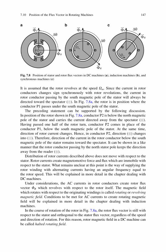
It is assumed that the rotor revolves at the speed Om. Since the current in rotor
conductors changes sign synchronously with rotor revolutions, the current in
rotor conductor passing by the south magnetic pole of the stator will always be
directed toward the spectator (). In Fig. 7.8a, the rotor is in position where the
conductor P1 passes under the south magnetic pole of the stator.
The preceding statement can be supported by the following discussion.
In position of the rotor shown in Fig. 7.8a, conductor P2 is below the north magnetic
pole of the stator and carries the current directed away from the spectator ().
Having passed one half of the rotor turn, conductor P2 comes in place of the
conductor P1, below the south magnetic pole of the stator. At the same time,
direction of rotor current changes. Hence, in conductor P2, direction () changes
into (). Therefore, direction of the current in the rotor conductor below the south
magnetic pole of the stator remains toward the spectator. It can be shown in a like
manner that the rotor conductor passing by the north stator pole keeps the direction
away from the reader ().
Distribution of rotor currents described above does not move with respect to the
stator. Rotor currents create magnetomotive force and flux which are immobile with
respect to the stator. What remains unclear at this point is the way of supplying the
rotor winding with alternating currents having an angular frequency equal to
the rotor speed. This will be explained in more detail in the chapter dealing with
DC machines.
Under considerations, the AC currents in rotor conductors create rotor flux
vector FR which revolves with respect to the rotor itself. The magnetic field
which rotates with respect to the originating windings is called rotating or revolvingmagnetic field. Conditions to be met for AC currents to create rotating magnetic
field will be explained in more detail in the chapter dealing with induction
machines.
In the course of rotation of the rotor in Fig. 7.8a, the rotor flux vector is still with
respect to the stator and orthogonal to the stator flux vector, regardless of the speed
and direction of rotation. For this reason, rotor magnetic field in a DC machine can
be called halted rotating field.
Fig. 7.8 Position of stator and rotor flux vectors in DC machines (a), induction machines (b), and
synchronous machines (c)
7.10 Position of the Flux Vector in Rotating Machines 147
Induction machines have AC currents of angular frequency o1 in stator
conductors. In rotor conductors, there are AC currents with different angular
frequency (o2). A simplified representation of an induction machine having one
pair of magnetic poles (p ¼ 1) is shown in Fig. 7.8b. By the previous example of a
DC machine, it is shown that AC currents in rotor conductors create rotor magnetic
field and rotor flux vector which rotate with respect to the rotor. The speed of
rotation of the flux vector with respect to the originating winding is determined by
the angular frequency of the winding currents.
In a like manner, stator flux FS in an induction machine rotates at a speed
O1 ¼ o1 with respect to the stator, while rotor flux FR rotates at a speed O2 ¼ o2
with respect to the rotor. Since the rotor revolves at the speed4 Om ¼ om, the
speed of rotation of rotor flux is Om + o2. Vector of the stator flux rotates at
the speed of o1; thus, the speed difference between stator flux vector and rotor
flux vector is o1 � Om � o2. According to (7.11) which gives the condition for
delivering the power and torquewith nonzero average values, the sumo1�Om�o2
must be equal to zero.
On the basis of previous considerations regarding the operation of induction
machines, the following conclusions can be drawn:
• The stator and rotor flux vectors rotate at the same speed. The speed of rotation
of the magnetic field in induction machine is O1, and it is determined by the
angular frequency o1 of the stator currents. In a two-pole machine, this speed is
O1 ¼ o1.
• Angle Dy between the stator and rotor flux vectors is constant in a steady state.
Machine provides electromagnetic torque proportional to sin(Dy), and it is
constant in a steady state.
• Rotor of a two-pole machine revolves at the speed which is different than the
speed O1 ¼ o1 of the magnetic field. The speed difference o2 ¼ o1 � Om is
called slip. Slip of a two-pole induction machine (p ¼ 1) is equal to the angular
frequency of the rotor currents (o2).
Synchronous machines have AC currents of frequency o1 in the stator windings
and a DC current in the rotor windings.5 The stator flux vector FS of a two-pole
(p ¼ 1) machine rotates at the speed O1 ¼ o1 with respect to the stator, while the
rotor flux vector FR rotates at the same speed as the rotor, Om ¼ om. A simplified
representation of a two-pole synchronous machine is shown in Fig. 7.8c. Genera-
tion of the electromagnetic torque with a nonzero average value requires that
relative position of the two flux vectors does not change. In other words, the
angle Dy has to remain constant. For this reason, the rotor speed and the speed of
4 Example in Fig. 7.8b considers a two-pole machine having p ¼ 1 pair of magnetic poles. Due to
o ¼ pO and p ¼ 1, mechanical speed (angular frequency) O corresponds to electrical speed
(angular frequency) o.5 There exist synchronous machines that have permanent magnets in place of DC excited rotor
windings.
148 7 Single-Fed and Double-Fed Converters
revolving stator flux vector have to be the same. Therefore, the stator and rotor flux
vectors of a synchronous machine rotate synchronously with the rotor. In a two-pole
synchronous machine, angular frequency of stator currents has to be equal to the
rotor speed. In machines having several pole pairs (p > 1), this condition takes the
form o1 ¼ pOm.
7.11 Rotating Field
The analysis carried out in the preceding subsection shows that the condition for
developing an electromagnetic torque with a nonzero average value is that relative
position Dy between the stator and rotor flux vectors remains constant. In DC
machines, both fluxes are still with respect to the stator, while in AC machines,
induction and synchronous, the two fluxes revolve at the same speed.
With the rotor revolving at a speed Om, the angle Dy can remain constant
provided that at least one of the two fluxes (FS or FR) revolves with respect to
the winding whose magnetomotive force originates the flux. The magnetic field
which rotates with respect to the originating winding is called rotating magneticfield. It will be shown later that creation of a rotating field in induction and
synchronous machines requires at least two separate windings on the stator, also
called phases or phase windings. With two-phase windings on the stator, the spatial
displacement between the winding axes has to be p/2. The alternating currents in
two-phase windings have to be of the same amplitude and the same angular
frequency. The difference of their initial phases has to be p/2, the same as the
spatial displacement between the phase windings. In this case, stator currents result
in a rotating magnetic field. The amplitude of the stator flux and its speed of rotation
can be changed by varying the amplitude and frequency of the stator currents.
In this chapter, an introductory example is given, illustrating the generation of a
rotating field by the stator with two-phase windings.
Figure 7.9 shows two stator windings with their magnetic axes spatially
displaced by p/2. Axes of the windings are denoted by a and b. The winding in
axis a has the same number of turns as the winding in axis b. Both windings carry
alternating currents of the same amplitude Im and frequency oS,
iaðtÞ ¼ Im cos oStð Þ;ibðtÞ ¼ Im cos oSt� p
2
� �¼ Im sin oStð Þ;
but their initial phases differ by p/2. Each winding creates a magnetomotive force
along its own axis. Magnetomotive force amplitude depends on the current and the
number of turns. The winding flux is proportional to the magnetomotive force and
inversely proportional to magnetic resistance. If magnetic circuits of the stator and
rotor are of cylindrical shape, magnetic resistance Rm incurred along the flux path
7.11 Rotating Field 149
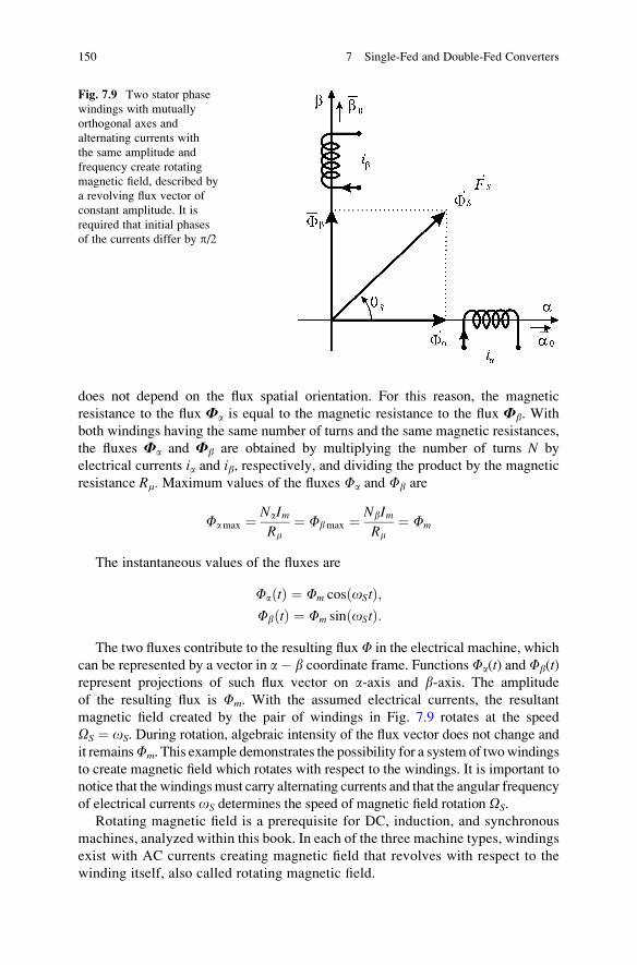
does not depend on the flux spatial orientation. For this reason, the magnetic
resistance to the flux Fa is equal to the magnetic resistance to the flux Fb. With
both windings having the same number of turns and the same magnetic resistances,
the fluxes Fa and Fb are obtained by multiplying the number of turns N by
electrical currents ia and ib, respectively, and dividing the product by the magnetic
resistance Rm. Maximum values of the fluxes Fa and Fb are
Famax ¼ NaImRm
¼ Fbmax ¼ NbImRm
¼ Fm
The instantaneous values of the fluxes are
FaðtÞ ¼ Fm cos oStð Þ;FbðtÞ ¼ Fm sin oStð Þ:
The two fluxes contribute to the resulting flux F in the electrical machine, which
can be represented by a vector in a� b coordinate frame. Functions Fa(t) and Fb(t)represent projections of such flux vector on a-axis and b-axis. The amplitude
of the resulting flux is Fm. With the assumed electrical currents, the resultant
magnetic field created by the pair of windings in Fig. 7.9 rotates at the speed
OS ¼ oS. During rotation, algebraic intensity of the flux vector does not change and
it remainsFm. This example demonstrates the possibility for a system of twowindings
to create magnetic field which rotates with respect to the windings. It is important to
notice that the windingsmust carry alternating currents and that the angular frequency
of electrical currents oS determines the speed of magnetic field rotation OS.
Rotating magnetic field is a prerequisite for DC, induction, and synchronous
machines, analyzed within this book. In each of the three machine types, windings
exist with AC currents creating magnetic field that revolves with respect to the
winding itself, also called rotating magnetic field.
Fig. 7.9 Two stator phase
windings with mutually
orthogonal axes and
alternating currents with
the same amplitude and
frequency create rotating
magnetic field, described by
a revolving flux vector of
constant amplitude. It is
required that initial phases
of the currents differ by p/2
150 7 Single-Fed and Double-Fed Converters
7.12 Types of Electrical Machines
7.12.1 Direct Current Machines
Electrical machines where the stator winding carries a DC current, while the rotor
winding carries AC currents, and where the stator flux vector and the rotor flux
vector do not move with respect to the stator are calledDC current machines. Statorwindings of DC machines are fed by DC, direct current. Rotor conductors in such
machines carry AC currents with the frequency determined by the speed of rotation.
The power source feeding a DC machine does not provide AC currents and
voltages, but instead it gives DC currents and voltages. The method of directing
DC current from the power source into the rotor conductors involves commutator,mechanical device explained further on. The action of commutator is such it
receives DC source current and feeds the rotor winding with AC currents, the
frequency of which is determined by the rotor speed.
Induction and synchronous machines have AC currents in their stator windings.
The angular frequency o1 of these currents provides a rotating magnetic field.
Therefore, these machines belong to the group of AC machines. The speed of
rotation of the magnetic field is determined by the angular frequency o1. It is
shown by the analysis of the structure in Fig. 7.9 that a system of two orthogonal
stator windings could create magnetic field that revolves at the speed determined by
the angular frequency of AC currents. Practical AC machines usually have a system
of stator windings consisting of three parts, three phases, that is, three-phasewindings. Magnetic axes of three-phase windings are spatially shifted by 2p/3.The initial phases of AC currents carried by the windings should be displaced by
2p/3 in order to provide rotating field. Amplitude Im of AC currents determines the
algebraic intensity of the flux vector, while the angular frequency o1 ¼ oS
determines the speed of rotation OS of the magnetic field.
7.12.2 Induction Machines
In addition to AC currents carried by the stator windings, induction machines
also have AC currents in the rotor conductors. Magnetic field created by the
stator currents rotates at the speed O1 ¼ o1, while the rotor field revolves at the
speed O2 ¼ o2 with respect to the rotor. The speeds of rotation of the stator and
rotor flux vectors have been discussed in the previous section, where it is shown
that the angular frequency of rotor currents, also called the slip frequency,
corresponds to the difference between the angular frequency of stator currents
and the rotor speed.
7.12 Types of Electrical Machines 151
7.12.3 Synchronous Machines
Like induction machines, synchronous machines have a system of stator windings
with AC currents creating magnetic field which revolves at the speed determined
by the angular frequency of stator currents. Currents of the rotor winding of a
synchronous machine are constant. They are supplied from a separate DC current
source. Rotor current creates the rotor flux which does not move with respect to the
rotor. Therefore, the rotor flux rotates together with the rotor and has the same speed
Om. There are synchronous machines which do not have the rotor winding. Instead,
the rotor flux is obtained by placing permanent magnets within the rotor magnetic
circuit. It has been shown before that the torque generation within an electrical
machine requires the angle between the stator and rotor flux vectors to be constant.
Therefore, the stator flux vector of a synchronous machine has to rotate at the same
speed as the rotor. In other words, the stator flux has to move synchronously with
the rotor.
Among these machines, each type has its merits, limitations, and specific field of
application.
Further analysis of electrical machines requires some basic knowledge on the
machine windings, skills in analyzing the magnetic field in the air gap, and
understanding the principles of rotating magnetic field.
152 7 Single-Fed and Double-Fed Converters
Chapter 8
Magnetic Field in the Air Gap
This chapter presents an analysis of the magnetic and electrical fields in the air gap
of a cylindrical machine. It is assumed that the fields come as a consequence of
electrical current in the windings. The magnetic field in the air gap is created by the
currents in both stator and rotor, which generate the corresponding stator and rotor
magnetomotive forces.
Conductors of the stator winding are placed in the grooves made on the inner
surface of the stator magnetic circuit, while conductors of the rotor winding are
placed in the grooves made on the outer surface of the rotor magnetic circuit. The
grooves are called slots, and they are opened toward the air gap (Fig. 8.1). Thus,
the conductors are placed near the air gap.
It is also assumed that conductors that make up a winding are many and that they
are series connected. They are not located in the same slot. Instead, the conductors
are distributed along the circumference of the air gap. Conductor density can be
determined by counting the number of conductors distributed along one unit length
of the circumference. To begin with, it is assumed that the windings are formed with
sinusoidal distribution of conductor density. Namely, the number of conductors
placed in the fragment R�Dy of the circumference (Fig. 8.2) is determined by the
function cosy, where the angle y determines the position of the observed fragment.
When electrical currents are fed into the winding, they create a sinusoidal distributed
current sheet, also called sinusoidally distributed current sheet. With these
assumptions, the subsequent analysis determines expressions for radial and tangen-
tial components of the magnetic field in the air gap, for magnetomotive forces of
the stator and rotor windings, and for fluxes per turn and the winding fluxes. The
subsequent passages also introduce the notation aimed to simplify the presentation
of the windings, magnetomotive forces, and fluxes. At the same time, the energy of
the magnetic field in the air gap and electromagnetic torque are calculates as well,
the torque being a measure of mechanical interaction between the stator and rotor.
Further on, relation between the torque and machine dimensions is analyzed.
Eventually, conditions for creating rotating magnetic field in the air gap are studied
and specified.
S.N. Vukosavic, Electrical Machines, Power Electronics and Power Systems,
DOI 10.1007/978-1-4614-0400-2_8, # Springer Science+Business Media New York 2013
153
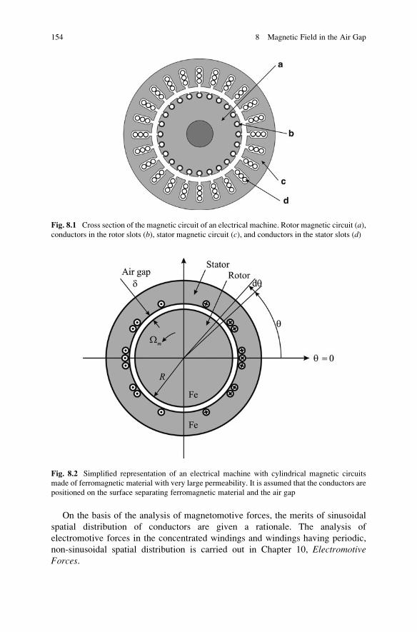
On the basis of the analysis of magnetomotive forces, the merits of sinusoidal
spatial distribution of conductors are given a rationale. The analysis of
electromotive forces in the concentrated windings and windings having periodic,
non-sinusoidal spatial distribution is carried out in Chapter 10, ElectromotiveForces.
Fig. 8.1 Cross section of the magnetic circuit of an electrical machine. Rotor magnetic circuit (a),conductors in the rotor slots (b), stator magnetic circuit (c), and conductors in the stator slots (d)
Fig. 8.2 Simplified representation of an electrical machine with cylindrical magnetic circuits
made of ferromagnetic material with very large permeability. It is assumed that the conductors are
positioned on the surface separating ferromagnetic material and the air gap
154 8 Magnetic Field in the Air Gap
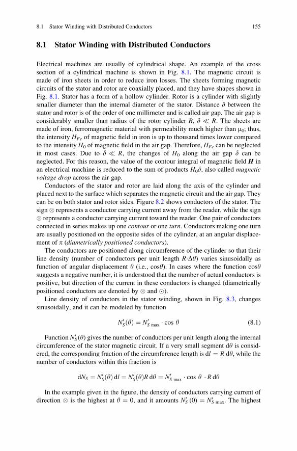
8.1 Stator Winding with Distributed Conductors
Electrical machines are usually of cylindrical shape. An example of the cross
section of a cylindrical machine is shown in Fig. 8.1. The magnetic circuit is
made of iron sheets in order to reduce iron losses. The sheets forming magnetic
circuits of the stator and rotor are coaxially placed, and they have shapes shown in
Fig. 8.1. Stator has a form of a hollow cylinder. Rotor is a cylinder with slightly
smaller diameter than the internal diameter of the stator. Distance d between the
stator and rotor is of the order of one millimeter and is called air gap. The air gap is
considerably smaller than radius of the rotor cylinder R, d � R. The sheets are
made of iron, ferromagnetic material with permeability much higher than m0; thus,the intensity HFe of magnetic field in iron is up to thousand times lower compared
to the intensity H0 of magnetic field in the air gap. Therefore, HFe can be neglected
in most cases. Due to d � R, the changes of H0 along the air gap d can be
neglected. For this reason, the value of the contour integral of magnetic field H in
an electrical machine is reduced to the sum of products H0d, also called magneticvoltage drop across the air gap.
Conductors of the stator and rotor are laid along the axis of the cylinder and
placed next to the surface which separates the magnetic circuit and the air gap. They
can be on both stator and rotor sides. Figure 8.2 shows conductors of the stator. The
sign� represents a conductor carrying current away from the reader, while the sign
� represents a conductor carrying current toward the reader. One pair of conductors
connected in series makes up one contour or one turn. Conductors making one turn
are usually positioned on the opposite sides of the cylinder, at an angular displace-
ment of p (diametrically positioned conductors).The conductors are positioned along circumference of the cylinder so that their
line density (number of conductors per unit length R�Dy) varies sinusoidally as
function of angular displacement y (i.e., cosy). In cases where the function cosysuggests a negative number, it is understood that the number of actual conductors is
positive, but direction of the current in these conductors is changed (diametrically
positioned conductors are denoted by � and �).
Line density of conductors in the stator winding, shown in Fig. 8.3, changes
sinusoidally, and it can be modeled by function
N0S yð Þ ¼ N0
S max � cos y (8.1)
Function NS0 (y) gives the number of conductors per unit length along the internal
circumference of the stator magnetic circuit. If a very small segment dy is consid-
ered, the corresponding fraction of the circumference length is dl ¼ R dy, while thenumber of conductors within this fraction is
dNS ¼ N0S yð Þ dl ¼ N0
S yð ÞR dy ¼ N0S max � cos y � R dy
In the example given in the figure, the density of conductors carrying current of
direction � is the highest at y ¼ 0, and it amounts NS0 (0) ¼ NS
0max. The highest
8.1 Stator Winding with Distributed Conductors 155
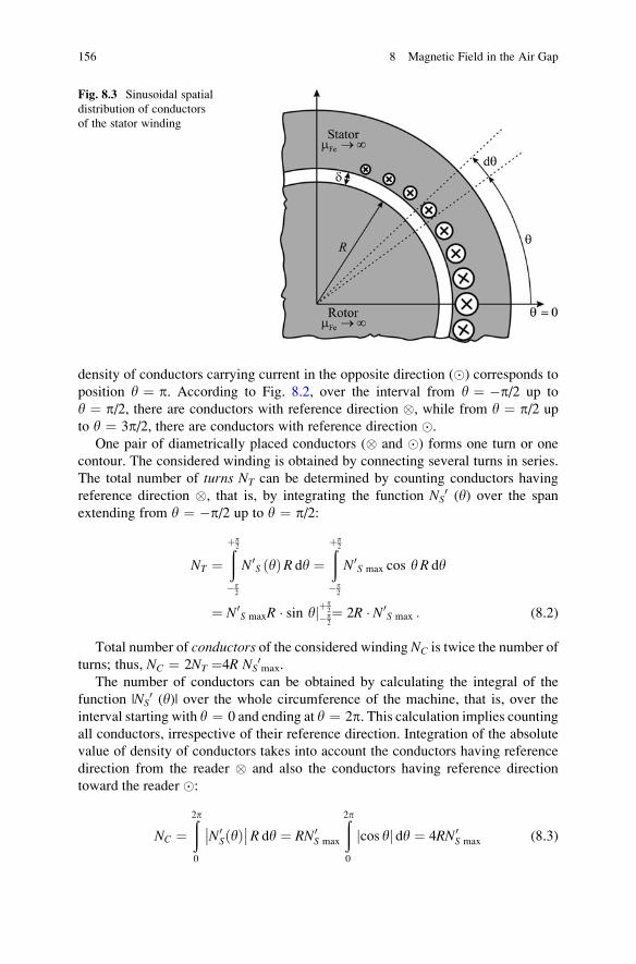
density of conductors carrying current in the opposite direction (�) corresponds to
position y ¼ p. According to Fig. 8.2, over the interval from y ¼ �p/2 up to
y ¼ p/2, there are conductors with reference direction �, while from y ¼ p/2 up
to y ¼ 3p/2, there are conductors with reference direction �.
One pair of diametrically placed conductors (� and �) forms one turn or one
contour. The considered winding is obtained by connecting several turns in series.
The total number of turns NT can be determined by counting conductors having
reference direction �, that is, by integrating the function NS0 (y) over the span
extending from y ¼ �p/2 up to y ¼ p/2:
NT ¼ðþp2
�p2
N0S yð ÞR dy ¼
ðþp2
�p2
N0S max cos yR dy
¼ N0S maxR � sin yjþp
2
�p2¼ 2R � N0
S max : (8.2)
Total number of conductors of the considered winding NC is twice the number of
turns; thus, NC ¼ 2NT ¼4R NS0max.
The number of conductors can be obtained by calculating the integral of the
function |NS0 (y)| over the whole circumference of the machine, that is, over the
interval starting with y ¼ 0 and ending at y ¼ 2p. This calculation implies counting
all conductors, irrespective of their reference direction. Integration of the absolute
value of density of conductors takes into account the conductors having reference
direction from the reader � and also the conductors having reference direction
toward the reader �:
NC ¼ð2p
0
N0S yð Þ�� ��R dy ¼ RN0
S max
ð2p
0
cos yj j dy ¼ 4RN0S max (8.3)
Fig. 8.3 Sinusoidal spatial
distribution of conductors
of the stator winding
156 8 Magnetic Field in the Air Gap
8.2 Sinusoidal Current Sheet
Electrical current in series-connected, spatially distributed stator conductors forms
a current sheet on the inner surface of the stator cylinder. Current direction from the
reader � extends in the interval �p/2 < y < p/2, while the direction toward the
reader � extends over the interval p/2 < y< 3p/2. Distribution of current over thissurface is shown in Fig. 8.2.
The considered current sheet has the line density of surface currents dependent
on the line density of conductors. The line density of the current sheet over the inner
surface of the stator cylinder is denoted by JS(y), and it is function of the angular
displacement y. It is determined by the density of conductors N0S(y) and the current
strength in a single conductor. Since the stator winding is formed by connecting the
conductors in series, all the conductors carry the same current i1(t), also called
the stator current. Current through conductors is determined by the reference
direction, shown in Fig. 8.2, and algebraic intensity i1(t) of the current supplied to
the winding at the two winding ends, also called terminals. Line density of the
surface currents is determined by (8.4):
JS yð Þ ¼ N0S yð Þ � i1 ¼ N0
S max � i1ð Þ cos y (8.4)
If the maximum line current density is denoted by
JS0 ¼ N0S max � i1
one obtains
JS yð Þ ¼ JS0 cos y (8.5)
Considering a small segment dy, the corresponding part of the circumference is
dl ¼ R dy, and the total current within this segment is
di ¼ JS yð ÞR dy
Electrical currents in axially placed conductors create magnetic field within the
machine. By considering the boundary surface between the air gap and magnetic
circuit made of iron (ferromagnetic), it can be noted that the magnetic flux entering
ferromagnetic material from the air gap does not change its value; thus, the
orthogonal components of magnetic induction B in the air (B0) and the ferromag-
netic material (BFe) are equal. Since permeability mFe of the ferromagnetic material
is considerably higher than permeability m0 of the air, it is justifiable to neglect the
field HFe in the ferromagnetic material and consider that field H exists only in
the air gap.
8.2 Sinusoidal Current Sheet 157
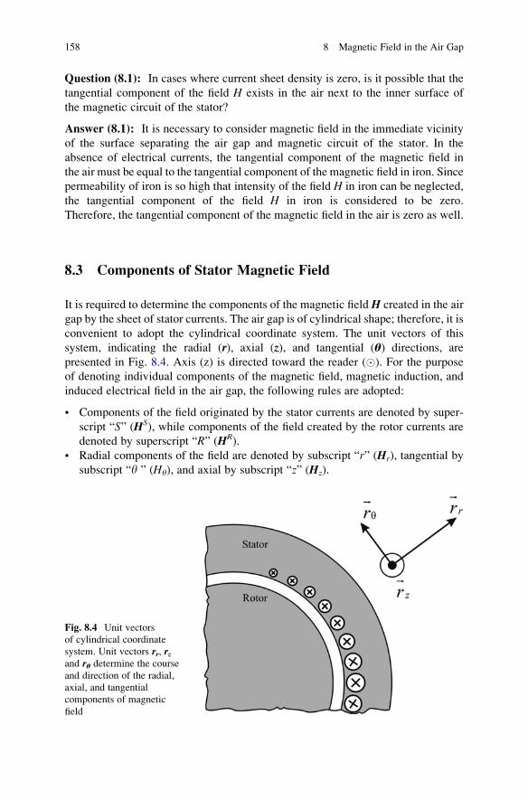
Question (8.1): In cases where current sheet density is zero, is it possible that the
tangential component of the field H exists in the air next to the inner surface of
the magnetic circuit of the stator?
Answer (8.1): It is necessary to consider magnetic field in the immediate vicinity
of the surface separating the air gap and magnetic circuit of the stator. In the
absence of electrical currents, the tangential component of the magnetic field in
the air must be equal to the tangential component of the magnetic field in iron. Since
permeability of iron is so high that intensity of the field H in iron can be neglected,
the tangential component of the field H in iron is considered to be zero.
Therefore, the tangential component of the magnetic field in the air is zero as well.
8.3 Components of Stator Magnetic Field
It is required to determine the components of the magnetic fieldH created in the air
gap by the sheet of stator currents. The air gap is of cylindrical shape; therefore, it is
convenient to adopt the cylindrical coordinate system. The unit vectors of this
system, indicating the radial (r), axial (z), and tangential (u) directions, are
presented in Fig. 8.4. Axis (z) is directed toward the reader (�). For the purpose
of denoting individual components of the magnetic field, magnetic induction, and
induced electrical field in the air gap, the following rules are adopted:
• Components of the field originated by the stator currents are denoted by super-
script “S” (HS), while components of the field created by the rotor currents are
denoted by superscript “R” (HR).
• Radial components of the field are denoted by subscript “r” (Hr), tangential by
subscript “y ” (Hy), and axial by subscript “z” (Hz).
Fig. 8.4 Unit vectors
of cylindrical coordinate
system. Unit vectors rr, rzand ru determine the course
and direction of the radial,
axial, and tangential
components of magnetic
field
158 8 Magnetic Field in the Air Gap
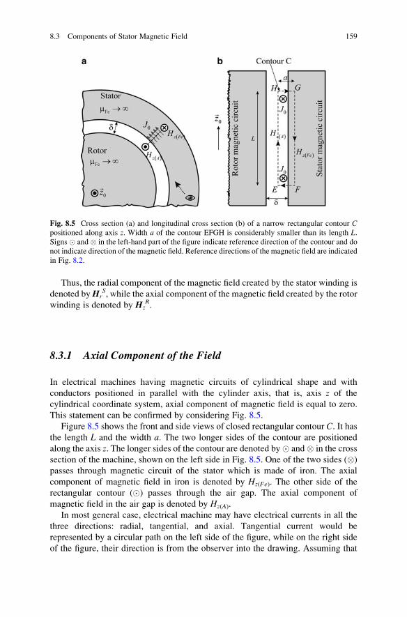
Thus, the radial component of the magnetic field created by the stator winding is
denoted byHrS, while the axial component of the magnetic field created by the rotor
winding is denoted by HzR.
8.3.1 Axial Component of the Field
In electrical machines having magnetic circuits of cylindrical shape and with
conductors positioned in parallel with the cylinder axis, that is, axis z of the
cylindrical coordinate system, axial component of magnetic field is equal to zero.
This statement can be confirmed by considering Fig. 8.5.
Figure 8.5 shows the front and side views of closed rectangular contour C. It hasthe length L and the width a. The two longer sides of the contour are positioned
along the axis z. The longer sides of the contour are denoted by� and� in the cross
section of the machine, shown on the left side in Fig. 8.5. One of the two sides (�)
passes through magnetic circuit of the stator which is made of iron. The axial
component of magnetic field in iron is denoted by Hz(Fe). The other side of the
rectangular contour (�) passes through the air gap. The axial component of
magnetic field in the air gap is denoted by Hz(A).
In most general case, electrical machine may have electrical currents in all the
three directions: radial, tangential, and axial. Tangential current would be
represented by a circular path on the left side of the figure, while on the right side
of the figure, their direction is from the observer into the drawing. Assuming that
Fig. 8.5 Cross section (a) and longitudinal cross section (b) of a narrow rectangular contour Cpositioned along axis z. Width a of the contour EFGH is considerably smaller than its length L.Signs � and � in the left-hand part of the figure indicate reference direction of the contour and do
not indicate direction of the magnetic field. Reference directions of the magnetic field are indicated
in Fig. 8.2.
8.3 Components of Stator Magnetic Field 159
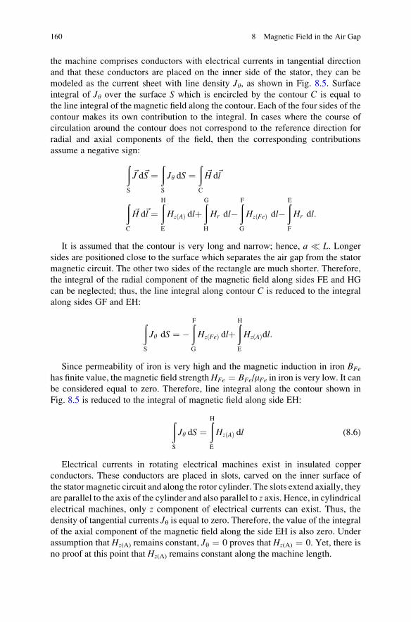
the machine comprises conductors with electrical currents in tangential direction
and that these conductors are placed on the inner side of the stator, they can be
modeled as the current sheet with line density Jy, as shown in Fig. 8.5. Surface
integral of Jy over the surface S which is encircled by the contour C is equal to
the line integral of the magnetic field along the contour. Each of the four sides of the
contour makes its own contribution to the integral. In cases where the course of
circulation around the contour does not correspond to the reference direction for
radial and axial components of the field, then the corresponding contributions
assume a negative sign:
ðS
~J d~S ¼ðS
Jy dS ¼ðC
~H d~l
ðC
~H d~l ¼ðH
E
HzðAÞ dlþðG
H
Hr dl�ðF
G
HzðFeÞ dl�ðE
F
Hr dl:
It is assumed that the contour is very long and narrow; hence, a � L. Longersides are positioned close to the surface which separates the air gap from the stator
magnetic circuit. The other two sides of the rectangle are much shorter. Therefore,
the integral of the radial component of the magnetic field along sides FE and HG
can be neglected; thus, the line integral along contour C is reduced to the integral
along sides GF and EH:
ðS
Jy dS ¼ �ðF
G
HzðFeÞ dlþðH
E
HzðAÞdl:
Since permeability of iron is very high and the magnetic induction in iron BFe
has finite value, the magnetic field strength HFe ¼ BFe/mFe in iron is very low. It canbe considered equal to zero. Therefore, line integral along the contour shown in
Fig. 8.5 is reduced to the integral of magnetic field along side EH:
ðS
Jy dS ¼ðH
E
HzðAÞ dl (8.6)
Electrical currents in rotating electrical machines exist in insulated copper
conductors. These conductors are placed in slots, carved on the inner surface of
the stator magnetic circuit and along the rotor cylinder. The slots extend axially, they
are parallel to the axis of the cylinder and also parallel to z axis. Hence, in cylindricalelectrical machines, only z component of electrical currents can exist. Thus, the
density of tangential currents Jy is equal to zero. Therefore, the value of the integralof the axial component of the magnetic field along the side EH is also zero. Under
assumption that Hz(A) remains constant, Jy ¼ 0 proves that Hz(A) ¼ 0. Yet, there is
no proof at this point that Hz(A) remains constant along the machine length.
160 8 Magnetic Field in the Air Gap
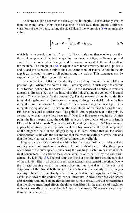
The contour C can be chosen in such way that its length L is considerably smaller
than the overall axial length of the machine. In such case, there are no significant
variations of the field Hz(A) along the side EH, and the expression (8.6) assumes the
value:
ðS
Jy dS ¼ 0 ¼ðH
E
HzðAÞ dl � HzðAÞL (8.7)
which leads to conclusion that Hz(A) ¼ 0. There is also another way to prove that
the axial component of the field is equal to zero. Statement Hz(A) ¼ 0 can be proved
even if the contour length L is longer and becomes comparable to the axial length of
the machine. The integral in (8.6) is equal to zero for an arbitrary choice of points H
and E, and this is possible only if the axial component of magnetic field in the air
gap Hz(A) is equal to zero at all points along the axis z. This statement can be
supported by the following consideration.
The contour C (EHGF) can be slightly extended by moving the side FE into
position F1E1, wherein the points E and E1 are very close. In such way, the contour
C1 is formed, defined by the points E1HGF1. In the absence of electrical currents in
tangential direction (Jy), the line integral of the field H along the contour C is equal
to zero. The same holds for the contour C1. For the reasons given above, the line
integral along the contour C reduces to the integral along the side EH, while the line
integral along the contour C1 reduces to the integral along the side E1H. Both
integrals are equal to zero. Therefore, the line integral of the field H along the side
EE1 has to be equal to zero as well. The point E1 can be placed next to the point E,
so that the changes in the field strength H from E to E1 become negligible. At this
point, the line integral along the side EE1 reduces to the product of the path length
EE1 and the field strength Hz(A) at the point E, leading to Hz(A) ¼ 0. This statement
applies for arbitrary choice of points E and E1. This proves that the axial component
of the magnetic field in the air gap is equal to zero. Notice that all the above
considerations start with the assumption that the machine cylinder is very long and
that the field changes at the ends of the cylinder are negligible.
Magnetic circuit of electrical machines has the stator hollow cylinder and the
rotor cylinder, both made of iron sheets. At both ends of the cylinder, the air gap
opens toward the outer space. Considering the windings, each turn has two diamet-
rical conductors. The ends of these conductors have to be tied by the end turns,
denoted by D in Fig. 5.6. The end turns are found at both the front and the rare side
of the cylinder. Electrical current in end turns extends in tangential direction. Due to
the air gap opening toward the outer space and due to end turns, there is local
dispersion of the flux at both ends of the machine in the vicinity of the air gap
opening. Therefore, a relatively small z component of the magnetic field may be
established toward the ends of cylindrical machines. Above-described end effectsand parasitic axial field are neglected throughout this book. It should be mentioned
that the above-mentioned effects should be considered in the analysis of machines
with an unusually small axial length L and with diameter 2R considerably larger
than the axial length L.
8.3 Components of Stator Magnetic Field 161
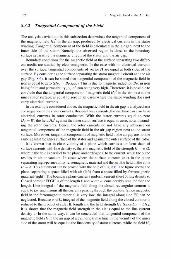
8.3.2 Tangential Component of the Field
The analysis carried out in this subsection determines the tangential component of
the magnetic field HyS in the air gap, produced by electrical currents in the stator
winding. Tangential component of the field is calculated in the air gap, next to the
inner side of the stator. Namely, the observed region is close to the boundary
surface separating the magnetic circuit of the stator and the air gap.
Boundary conditions for the magnetic field at the surface separating two differ-
ent media are studied by electromagnetic. In the case with no electrical currents
over the surface, tangential components of vector H are equal at both sides of the
surface. By considering the surface separating the stator magnetic circuit and the air
gap (Fig. 8.6), it can be stated that tangential component of the magnetic field in
iron is equal to zero (HFe ¼ BFe/mFe). This is due to magnetic induction BFe in iron
being finite and permeability mFe of iron being very high. Therefore, it is possible toconclude that the tangential component of magnetic field Hy
S in the air, next to the
inner stator surface, is equal to zero in all cases where the stator winding does not
carry electrical currents.
In the example considered above, the magnetic field in the air gap is analyzed as a
consequence of the stator currents. Besides these currents, the machine can also have
electrical currents in rotor conductors. With the stator currents equal to zero
(JS ¼ 0), the fieldHyS against the inner stator surface is equal to zero, notwithstand-
ing the rotor currents. Hence, the rotor currents do not have any influence on
tangential component of the magnetic field in the air gap region next to the stator
surface. Moreover, tangential components of magnetic field in the air gap are not the
same against the inner surface of the stator and against the outer surface of the rotor.
It is known that in close vicinity of a plane which carries a uniform sheet of
surface currents with line density s, there is magnetic field of the strengthH ¼ s /2,
wherein the field is parallel to the plane and orthogonal to the current, while the plane
resides in air or vacuum. In cases where the surface currents exist in the plane
separating high-permeability ferromagnetic material and the air, the field in the air is
H ¼ s. This statement can be proved with the help of Fig. 8.6. The figure shows the
plane separating a space filled with air (left) from a space filled by ferromagnetic
material (right). The boundary plane carries a uniform current sheet of line density s.Closed contour EFGH is of the length L and width a, considerably smaller than the
length. Line integral of the magnetic field along the closed rectangular contour is
equal to Ls, and it sums all the currents passing through the contour. Since magnetic
field in the ferromagnetic material is very low, the integral along side FG can be
neglected. Because a �L, integral of the magnetic field along the closed contour is
reduced to the product of side HE length and the field strengthHA. Since Ls ¼ LHA,
it is shown that the magnetic field strength in the air is equal to the line current
density s. In the same way, it can be concluded that tangential component of the
magnetic field Hy in the air gap of a cylindrical machine in the vicinity of the inner
side of the stator will be equal to the line density of stator currents, while the fieldHy
162 8 Magnetic Field in the Air Gap
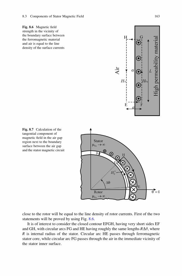
close to the rotor will be equal to the line density of rotor currents. First of the two
statements will be proved by using Fig. 8.6.
It is of interest to consider the closed contour EFGH, having very short sides EF
and GH, with circular arcs FG and HE having roughly the same lengths RDy, whereR is internal radius of the stator. Circular arc HE passes through ferromagnetic
stator core, while circular arc FG passes through the air in the immediate vicinity of
the stator inner surface.
Fig. 8.6 Magnetic field
strength in the vicinity of
the boundary surface between
the ferromagnetic material
and air is equal to the line
density of the surface currents
Fig. 8.7 Calculation of the
tangential component of
magnetic field in the air gap
region next to the boundary
surface between the air gap
and the stator magnetic circuit
8.3 Components of Stator Magnetic Field 163
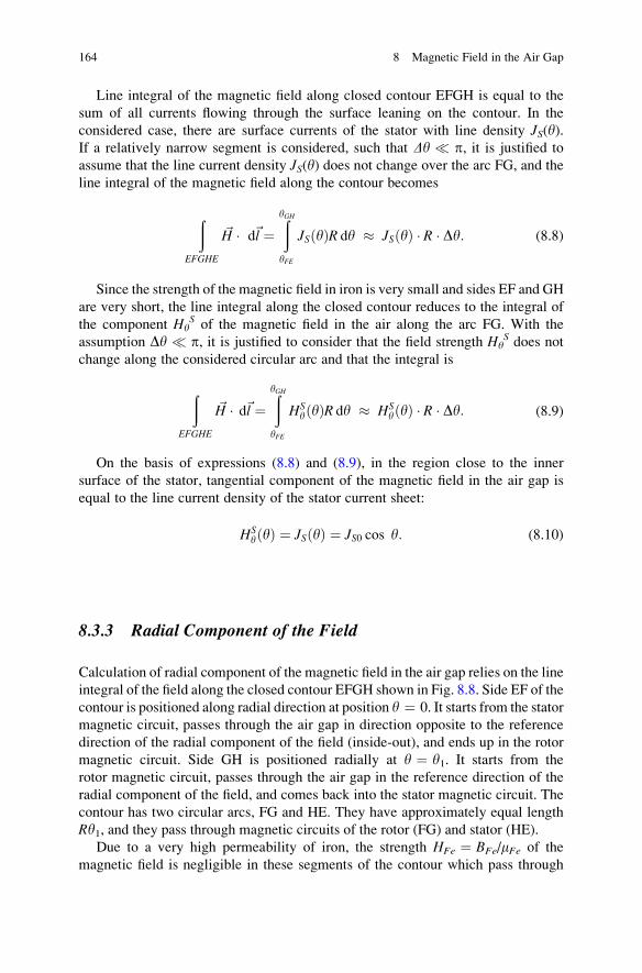
Line integral of the magnetic field along closed contour EFGH is equal to the
sum of all currents flowing through the surface leaning on the contour. In the
considered case, there are surface currents of the stator with line density JS(y).If a relatively narrow segment is considered, such that Dy � p, it is justified to
assume that the line current density JS(y) does not change over the arc FG, and the
line integral of the magnetic field along the contour becomes
ðEFGHE
~H � d~l ¼ðyGH
yFE
JS yð ÞR dy � JS yð Þ � R � Dy: (8.8)
Since the strength of the magnetic field in iron is very small and sides EF and GH
are very short, the line integral along the closed contour reduces to the integral of
the component HyS of the magnetic field in the air along the arc FG. With the
assumption Dy � p, it is justified to consider that the field strength HyS does not
change along the considered circular arc and that the integral is
ðEFGHE
~H � d~l ¼ðyGH
yFE
HSy yð ÞR dy � HS
y yð Þ � R � Dy: (8.9)
On the basis of expressions (8.8) and (8.9), in the region close to the inner
surface of the stator, tangential component of the magnetic field in the air gap is
equal to the line current density of the stator current sheet:
HSy yð Þ ¼ JS yð Þ ¼ JS0 cos y: (8.10)
8.3.3 Radial Component of the Field
Calculation of radial component of the magnetic field in the air gap relies on the line
integral of the field along the closed contour EFGH shown in Fig. 8.8. Side EF of the
contour is positioned along radial direction at position y ¼ 0. It starts from the stator
magnetic circuit, passes through the air gap in direction opposite to the reference
direction of the radial component of the field (inside-out), and ends up in the rotor
magnetic circuit. Side GH is positioned radially at y ¼ y1. It starts from the
rotor magnetic circuit, passes through the air gap in the reference direction of the
radial component of the field, and comes back into the stator magnetic circuit. The
contour has two circular arcs, FG and HE. They have approximately equal length
Ry1, and they pass through magnetic circuits of the rotor (FG) and stator (HE).
Due to a very high permeability of iron, the strength HFe ¼ BFe/mFe of the
magnetic field is negligible in these segments of the contour which pass through
164 8 Magnetic Field in the Air Gap
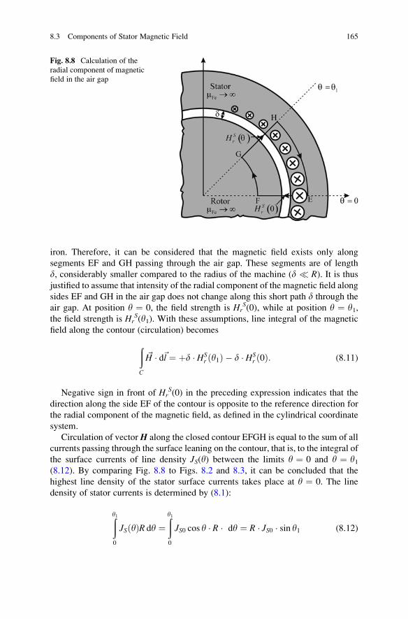
iron. Therefore, it can be considered that the magnetic field exists only along
segments EF and GH passing through the air gap. These segments are of length
d, considerably smaller compared to the radius of the machine (d � R). It is thusjustified to assume that intensity of the radial component of the magnetic field along
sides EF and GH in the air gap does not change along this short path d through the
air gap. At position y ¼ 0, the field strength is HrS(0), while at position y ¼ y1,
the field strength is HrS(y1). With these assumptions, line integral of the magnetic
field along the contour (circulation) becomes
ðC
~H � d~l ¼ þd � HSr ðy1Þ � d � HS
r ð0Þ: (8.11)
Negative sign in front of HrS(0) in the preceding expression indicates that the
direction along the side EF of the contour is opposite to the reference direction for
the radial component of the magnetic field, as defined in the cylindrical coordinate
system.
Circulation of vectorH along the closed contour EFGH is equal to the sum of all
currents passing through the surface leaning on the contour, that is, to the integral of
the surface currents of line density JS(y) between the limits y ¼ 0 and y ¼ y1(8.12). By comparing Fig. 8.8 to Figs. 8.2 and 8.3, it can be concluded that the
highest line density of the stator surface currents takes place at y ¼ 0. The line
density of stator currents is determined by (8.1):
ðy10
JS yð ÞR dy ¼ðy10
JS0 cos y � R � dy ¼ R � JS0 � sin y1 (8.12)
Fig. 8.8 Calculation of the
radial component of magnetic
field in the air gap
8.3 Components of Stator Magnetic Field 165
In position y1, the radial component of the air gap magnetic field caused by the
stator currents is equal to
HSr ðy1Þ ¼ HS
r ð0Þ þJS0R
dsin y1 (8.13)
In order to calculate radial component of the field, it is necessary to determine
the constant HrS(0).
In cases when the stator currents are absent (JS0 ¼ 0), expression (8.13) reduces
to HrS(y) ¼ Hr
S(0). With JS0 ¼ 0, the field caused by the stator currents should be
zero as well. This can be proved by the following consideration. If constantHrS(0) is
positive while JS0 ¼ 0, radial component of the magnetic field in the air gap does not
change along the machine circumference, and it is directed from rotor toward stator.
On these grounds, it is possible to show that constant HrS(0) has to be equal to zero.
In courses on Electrical Engineering Fundamentals and Electromagnetics, it is
shown that the flux of the vector B which comes out of a closed surface S must
be equal to zero. An example of the closed surface S can be the one enveloping the
rotor of an electrical machine. This surface has three parts, cylindrical surface
passing through the air gap and the two flat, round parts at both machine ends,
representing the bases of the cylinder. The flux of the vector B through the surface Sis called the output flux, and it is calculated according to
þS
~B � d~S ¼ 0
Differential form of the preceding statement is
div ~B ¼ 0;
and it represents one out of four Maxwell equations. Divergence is a spatial
derivative of a vector which can be used for establishing the relation between the
surface integral (2D) of the vector over a closed surface S and the space integral
(3D) of the spatial derivative of the same vector within the domain encircled by the
closed surface S. Therefore, the information on the divergence of vector B in
domain V, encircled by surface S, can be used to calculate the output flux of the
vector B:
þS
~B � d~S ¼ðV
div ~B dV:
As a consequence of div B ¼ 0, the surface integral of vector B over the close
surface S is equal to zero:
þS
~B � d~S ¼ 0: (8.14)
166 8 Magnetic Field in the Air Gap
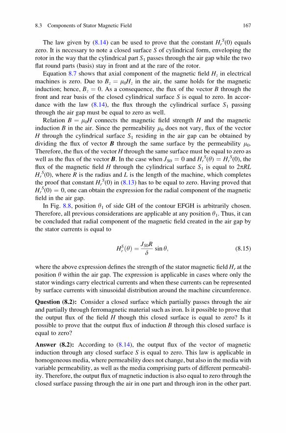
The law given by (8.14) can be used to prove that the constant HrS(0) equals
zero. It is necessary to note a closed surface S of cylindrical form, enveloping the
rotor in the way that the cylindrical part S1 passes through the air gap while the twoflat round parts (basis) stay in front and at the rare of the rotor.
Equation 8.7 shows that axial component of the magnetic field Hz in electrical
machines is zero. Due to Bz ¼ m0Hz in the air, the same holds for the magnetic
induction; hence, Bz ¼ 0. As a consequence, the flux of the vector B through the
front and rear basis of the closed cylindrical surface S is equal to zero. In accor-
dance with the law (8.14), the flux through the cylindrical surface S1 passing
through the air gap must be equal to zero as well.
Relation B ¼ m0H connects the magnetic field strength H and the magnetic
induction B in the air. Since the permeability m0 does not vary, flux of the vector
H through the cylindrical surface S1 residing in the air gap can be obtained by
dividing the flux of vector B through the same surface by the permeability m0.Therefore, the flux of the vectorH through the same surface must be equal to zero as
well as the flux of the vector B. In the case when JS0 ¼ 0 and HrS(y) ¼ Hr
S(0), the
flux of the magnetic field H through the cylindrical surface S1 is equal to 2pRLHr
S(0), where R is the radius and L is the length of the machine, which completes
the proof that constant HrS(0) in (8.13) has to be equal to zero. Having proved that
HrS(0) ¼ 0, one can obtain the expression for the radial component of the magnetic
field in the air gap.
In Fig. 8.8, position y1 of side GH of the contour EFGH is arbitrarily chosen.
Therefore, all previous considerations are applicable at any position y1. Thus, it canbe concluded that radial component of the magnetic field created in the air gap by
the stator currents is equal to
HSr ðyÞ ¼
JS0R
dsin y; (8.15)
where the above expression defines the strength of the stator magnetic fieldHr at the
position y within the air gap. The expression is applicable in cases where only the
stator windings carry electrical currents and when these currents can be represented
by surface currents with sinusoidal distribution around the machine circumference.
Question (8.2): Consider a closed surface which partially passes through the air
and partially through ferromagnetic material such as iron. Is it possible to prove that
the output flux of the field H though this closed surface is equal to zero? Is it
possible to prove that the output flux of induction B through this closed surface is
equal to zero?
Answer (8.2): According to (8.14), the output flux of the vector of magnetic
induction through any closed surface S is equal to zero. This law is applicable in
homogeneousmedia, where permeability does not change, but also in themedia with
variable permeability, as well as the media comprising parts of different permeabil-
ity. Therefore, the output flux of magnetic induction is also equal to zero through the
closed surface passing through the air in one part and through iron in the other part.
8.3 Components of Stator Magnetic Field 167
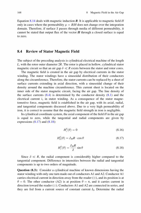
Equation 8.14 deals with magnetic induction B. It is applicable to magnetic field Honly in cases where the permeability m ¼ B/H does not change over the integration
domain. Therefore, if surface S passes through media of different permeability, it
cannot be stated that output flux of the vector H through a closed surface is equal
to zero.
8.4 Review of Stator Magnetic Field
The subject of the preceding analysis is cylindrical electrical machine of the length
L, with the rotor outer diameter 2R. The rotor is placed in hollow, cylindrical stator
magnetic circuit so that an air gap d � R exists between the stator and rotor cores.
The magnetic field is created in the air gap by electrical currents in the stator
winding. The stator windings have a sinusoidal distribution of their conductors
along the circumference. Therefore, the stator currents can be replaced by a sheet of
surface currents extending in axial direction, with a sinusoidal change of their
density around the machine circumference. This current sheet is located on the
inner side of the stator magnetic circuit, facing the air gap. The line density of
the surface currents (8.4) is determined by the conductor density (8.1) and the
electrical current i1 in stator winding. As a consequence of the stator magne-
tomotive force, magnetic field is established in the air gap, with its axial, radial,
and tangential components discussed above. Due to a very high permeability of
iron, it is correct to assume that the magnetic field strength in iron is negligible.
In cylindrical coordinate system, the axial component of the fieldH in the air gap
is equal to zero, while the tangential and radial components are given by
expressions (8.17) and (8.18):
HSz ðyÞ ¼ 0 (8.16)
HSyðyÞ ¼ JS0R � cos y (8.17)
HSr ðyÞ ¼
JS0R
dsin y (8.18)
Since d � R, the radial component is considerably higher compared to the
tangential component. Difference in intensities between the radial and tangential
components is up to two orders of magnitude.
Question (8.3): Consider a cylindrical machine of known dimensions having the
stator winding with only one turn made out of conductors A1 and A2. Conductor A1
carries electrical current in direction away from the reader (�), and its position is at
y ¼ 0. The other conductor (A2) is at position y ¼ p, and it carries current in
direction toward the reader (�). Conductors A1 and A2 are connected in series, and
they are fed from a current source of constant current I0. Determine the radial
168 8 Magnetic Field in the Air Gap
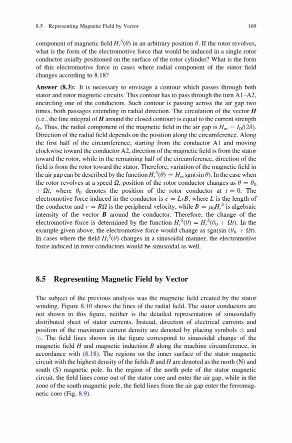
component of magnetic field HrS(y) in an arbitrary position y. If the rotor revolves,
what is the form of the electromotive force that would be induced in a single rotor
conductor axially positioned on the surface of the rotor cylinder? What is the form
of this electromotive force in cases where radial component of the stator field
changes according to 8.18?
Answer (8.3): It is necessary to envisage a contour which passes through both
stator and rotor magnetic circuits. This contour has to pass through the turn A1–A2,
encircling one of the conductors. Such contour is passing across the air gap two
times, both passages extending in radial direction. The circulation of the vector H(i.e., the line integral ofH around the closed contour) is equal to the current strength
I0. Thus, the radial component of the magnetic field in the air gap is Hm ¼ I0/(2d).Direction of the radial field depends on the position along the circumference. Along
the first half of the circumference, starting from the conductor A1 and moving
clockwise toward the conductor A2, direction of the magnetic field is from the stator
toward the rotor, while in the remaining half of the circumference, direction of the
field is from the rotor toward the stator. Therefore, variation of the magnetic field in
the air gap can be described by the functionHrS(y) ¼ Hm sgn(sin y). In the case when
the rotor revolves at a speed O, position of the rotor conductor changes as y ¼ y0þ Ot, where y0 denotes the position of the rotor conductor at t ¼ 0. The
electromotive force induced in the conductor is e ¼ LvB, where L is the length of
the conductor and v ¼ RO is the peripheral velocity, while B ¼ m0HrS is algebraic
intensity of the vector B around the conductor. Therefore, the change of the
electromotive force is determined by the function HrS(y) ¼ Hr
S(y0 þ Ot). In the
example given above, the electromotive force would change as sgn(sin (y0 þ Ot).In cases where the field Hr
S(y) changes in a sinusoidal manner, the electromotive
force induced in rotor conductors would be sinusoidal as well.
8.5 Representing Magnetic Field by Vector
The subject of the previous analysis was the magnetic field created by the stator
winding. Figure 8.10 shows the lines of the radial field. The stator conductors are
not shown in this figure, neither is the detailed representation of sinusoidally
distributed sheet of stator currents. Instead, direction of electrical currents and
position of the maximum current density are denoted by placing symbols � and
�. The field lines shown in the figure correspond to sinusoidal change of the
magnetic field H and magnetic induction B along the machine circumference, in
accordance with (8.18). The regions on the inner surface of the stator magnetic
circuit with the highest density of the fields B andH are denoted as the north (N) and
south (S) magnetic pole. In the region of the north pole of the stator magnetic
circuit, the field lines come out of the stator core and enter the air gap, while in the
zone of the south magnetic pole, the field lines from the air gap enter the ferromag-
netic core (Fig. 8.9).
8.5 Representing Magnetic Field by Vector 169
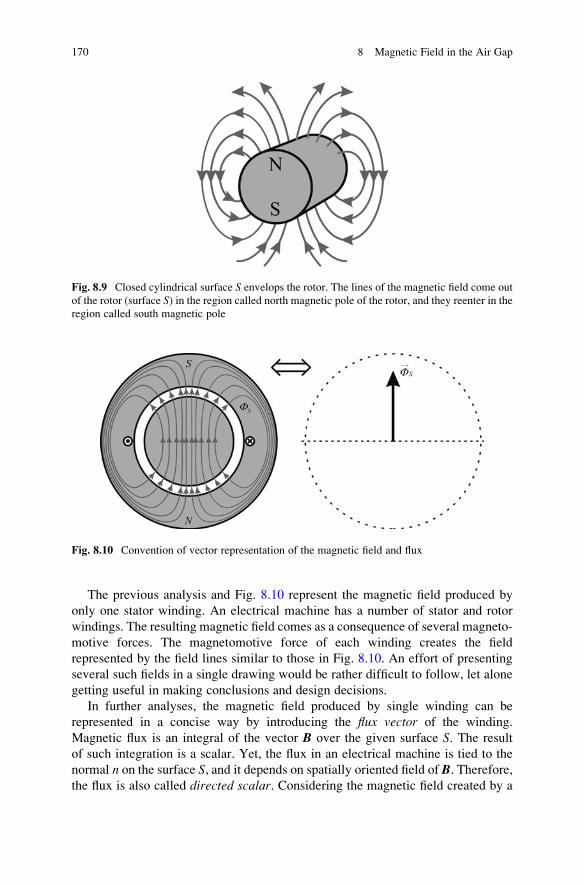
The previous analysis and Fig. 8.10 represent the magnetic field produced by
only one stator winding. An electrical machine has a number of stator and rotor
windings. The resulting magnetic field comes as a consequence of several magneto-
motive forces. The magnetomotive force of each winding creates the field
represented by the field lines similar to those in Fig. 8.10. An effort of presenting
several such fields in a single drawing would be rather difficult to follow, let alone
getting useful in making conclusions and design decisions.
In further analyses, the magnetic field produced by single winding can be
represented in a concise way by introducing the flux vector of the winding.
Magnetic flux is an integral of the vector B over the given surface S. The result
of such integration is a scalar. Yet, the flux in an electrical machine is tied to the
normal n on the surface S, and it depends on spatially oriented field of B. Therefore,the flux is also called directed scalar. Considering the magnetic field created by a
Fig. 8.10 Convention of vector representation of the magnetic field and flux
Fig. 8.9 Closed cylindrical surface S envelops the rotor. The lines of the magnetic field come out
of the rotor (surface S) in the region called north magnetic pole of the rotor, and they reenter in the
region called south magnetic pole
170 8 Magnetic Field in the Air Gap
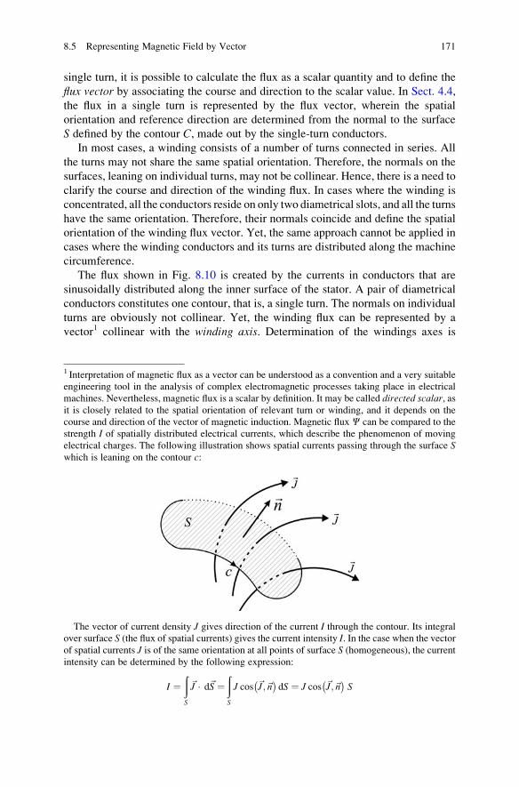
single turn, it is possible to calculate the flux as a scalar quantity and to define the
flux vector by associating the course and direction to the scalar value. In Sect. 4.4,
the flux in a single turn is represented by the flux vector, wherein the spatial
orientation and reference direction are determined from the normal to the surface
S defined by the contour C, made out by the single-turn conductors.
In most cases, a winding consists of a number of turns connected in series. All
the turns may not share the same spatial orientation. Therefore, the normals on the
surfaces, leaning on individual turns, may not be collinear. Hence, there is a need to
clarify the course and direction of the winding flux. In cases where the winding is
concentrated, all the conductors reside on only two diametrical slots, and all the turns
have the same orientation. Therefore, their normals coincide and define the spatial
orientation of the winding flux vector. Yet, the same approach cannot be applied in
cases where the winding conductors and its turns are distributed along the machine
circumference.
The flux shown in Fig. 8.10 is created by the currents in conductors that are
sinusoidally distributed along the inner surface of the stator. A pair of diametrical
conductors constitutes one contour, that is, a single turn. The normals on individual
turns are obviously not collinear. Yet, the winding flux can be represented by a
vector1 collinear with the winding axis. Determination of the windings axes is
1 Interpretation of magnetic flux as a vector can be understood as a convention and a very suitable
engineering tool in the analysis of complex electromagnetic processes taking place in electrical
machines. Nevertheless, magnetic flux is a scalar by definition. It may be called directed scalar, asit is closely related to the spatial orientation of relevant turn or winding, and it depends on the
course and direction of the vector of magnetic induction. Magnetic flux C can be compared to the
strength I of spatially distributed electrical currents, which describe the phenomenon of moving
electrical charges. The following illustration shows spatial currents passing through the surface Swhich is leaning on the contour c:
The vector of current density J gives direction of the current I through the contour. Its integral
over surface S (the flux of spatial currents) gives the current intensity I. In the case when the vectorof spatial currents J is of the same orientation at all points of surface S (homogeneous), the current
intensity can be determined by the following expression:
I ¼ðS
~J � d~S ¼ðS
J cos ~J;~n� �
dS ¼ J cos ~J;~n� �
S
8.5 Representing Magnetic Field by Vector 171
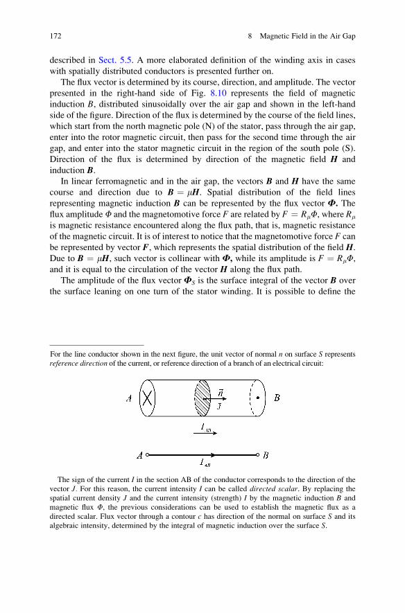
described in Sect. 5.5. A more elaborated definition of the winding axis in cases
with spatially distributed conductors is presented further on.
The flux vector is determined by its course, direction, and amplitude. The vector
presented in the right-hand side of Fig. 8.10 represents the field of magnetic
induction B, distributed sinusoidally over the air gap and shown in the left-hand
side of the figure. Direction of the flux is determined by the course of the field lines,
which start from the north magnetic pole (N) of the stator, pass through the air gap,
enter into the rotor magnetic circuit, then pass for the second time through the air
gap, and enter into the stator magnetic circuit in the region of the south pole (S).
Direction of the flux is determined by direction of the magnetic field H and
induction B.In linear ferromagnetic and in the air gap, the vectors B and H have the same
course and direction due to B ¼ mH. Spatial distribution of the field lines
representing magnetic induction B can be represented by the flux vector F. The
flux amplitude F and the magnetomotive force F are related by F ¼ RmF, where Rm
is magnetic resistance encountered along the flux path, that is, magnetic resistance
of the magnetic circuit. It is of interest to notice that the magnetomotive force F can
be represented by vector F, which represents the spatial distribution of the field H.
Due to B ¼ mH, such vector is collinear with F, while its amplitude is F ¼ RmF,and it is equal to the circulation of the vector H along the flux path.
The amplitude of the flux vector FS is the surface integral of the vector B over
the surface leaning on one turn of the stator winding. It is possible to define the
For the line conductor shown in the next figure, the unit vector of normal n on surface S represents
reference direction of the current, or reference direction of a branch of an electrical circuit:
The sign of the current I in the section AB of the conductor corresponds to the direction of the
vector J. For this reason, the current intensity I can be called directed scalar. By replacing the
spatial current density J and the current intensity (strength) I by the magnetic induction B and
magnetic flux F, the previous considerations can be used to establish the magnetic flux as a
directed scalar. Flux vector through a contour c has direction of the normal on surface S and its
algebraic intensity, determined by the integral of magnetic induction over the surface S.
172 8 Magnetic Field in the Air Gap
vector of the total winding fluxC as the sum of flux vectors representing the flux in
individual turns.2
Question (8.4): Consider Fig. 8.10, where symbols � and � denote direction of
current in conductors of the stator winding. There are 2NT conductors, sinusoidally
distributed along the machine circumference, all of them carrying electrical current
I. Derive the expression for the maximum value of the radial component HrS of the
air gap field which is achieved in the regions of the north and south magnetic poles
(use the previously obtained expressions and the relation between the maximum
line density of conductors NSmax and the total number of conductors, NT ¼ 2
RNSmax, H ¼ NTI/(2d)). Determine the amplitude of the stator magnetomotive
force F.
Answer (8.4): It is necessary to determine the line integral of the field H along the
closed contour starting from the north pole of the stator, going vertically toward the
south magnetic pole, and closing through the stator magnetic circuit. Circulation of
the vector H is NTI ¼ 2dH. Intensity of the magnetic field is Hmax ¼ NTI/(2d).Magnetomotive force F is equal to the circulation of the vector H, F ¼ NTI.
Question (8.5): Assume now that the number of stator conductors does not change
and that stator current is the same, but the conductors are grouped at the places
designated by � and � in Fig. 8.10. Instead of being distributed, the conductors are
concentrated in diametrical slots. Such winding is called concentrated winding.What is, in this case, the value of the line integral of the magnetic field H? Are thereany changes in the maximum intensity of the field H below the north and south
poles? What is the amplitude of the stator magnetomotive force F?
Answer (8.5): The magnetic field strength Hmax and the magnetomotive force Fare equal as in the preceding case, H ¼ NTI /(2d), F ¼ NTI.
Question (8.6): Compare the field distribution H(y) for concentrated and
distributed winding.
Answer (8.6): On the basis of the previous expressions, magnetic field of the
winding with sinusoidally distributed conductors has a sinusoidal distribution of
the magnetic field in the air gap. In the case when the conductors are concentrated,
radial component of magnetic field HrS(y) ¼ Hm sgn(sin y) has a constant ampli-
tude along the circumference, and its direction is positive over one half and
negative over the other half of the circumference. In both cases, maximum intensity
of the field is H ¼ NTI /(2d).
Question (8.7): Determine the flux through a contour made of two conductors
denoted by � and � in Fig. 8.10 in the case when the winding is concentrated and
has NT conductors. All conductors of the considered winding directed toward the
2 Total flux C of the stator winding with N turns, with sinusoidal distribution of conductors along
circumference of the stator, andwith fluxFS in one of the turns is not equal toNFS because the fluxes
of individual turns are not equal. Flux FS in a single turn (contour) is function of position y.
8.5 Representing Magnetic Field by Vector 173
reader are in position denoted by �. The remaining conductors of the opposite
direction are in position denoted by �.
Answer (8.7): It is necessary to note that the magnetic field strength in the air gap
is H ¼ þNTI/(2d) over the interval y ∈ [0. . .p] and H ¼ �NTI/(2d) over intervaly∈ [p. . .2p]. The flux through the contour is obtained by calculating the integral ofthe magnetic induction B over the surface leaning on the contour. Since the surface
integral of magnetic induction over a closed surface is equal to zero (div B ¼ 0),
the surface integral of B through all the surfaces leaning on the same contour is the
same. Therefore, there is a possibility of selecting the proper surface that would
facilitate the calculation. For the surface in the air gap, the expression for magnetic
induction B is known. Over the interval [0. . .p], the magnetic induction in the air
gap has radial direction and intensity B ¼ þm0NTI/(2d). The surface leaning on thecontour can be specified by the semicircular banded rectangle which leans on
conductor �, passes through the air gap over the arc interval [0. . .p], and leans
on conductor �, which is positioned at y ¼ p in Fig. 8.10. The considered surface
has the length L, width pR, and surface area S ¼ LpR. In all parts, the vector of
magnetic induction is vertical to the surface; thus, the flux through the surface, that
is, the flux through the contour, is equal to F ¼ BS ¼ m0 pLR NT I /(2d).
Question (8.8): Determine the flux of a contour consisting of two conductors
denoted by � and � in Fig. 8.8 in the case when the winding has a sinusoidal
distribution of conductors.
Answer (8.8): It is necessary to note that in the zones of magnetic poles, at
positions y ¼ p/2 and y ¼ 3p/2, the magnetic induction in the air gap is equal to
the one in the preceding case (Bmax ¼ þm0NTI/(2d)), but the field changes along thecircumference. As in the preceding case of Question 8.7, the flux through
the contour can be obtained by calculating the surface integral of the magnetic
induction over the semicircular banded rectangle of the length L and width pR,which passes through the air gap and leans on conductors � and �. The area of the
considered surface is S ¼ LpR. The flux cannot be calculated as BmaxS, as the
magnetic induction exhibits sinusoidal changes over the surface. The flux through
the contour is equal to the product BavS, where Bav is the average value of the
magnetic induction in the air gap over the interval y ∈ [0. . .p]. It is well knownthat the function sin(y) has an average value of 2/p on the interval y ∈ [0. . .p].Therefore, Bav ¼ 2/pBmax. The flux through the contour is F ¼ BavS ¼ m0 LRNT I /d.
Question (8.9): By using the results obtained in previous two questions, specify
how do the magnetomotive force of the winding and the flux in one contour change
by converting a concentrated winding into winding with sinusoidal distribution of
conductors. Are there any reasons in favor of using distributed windings?
Answer (8.9): If the twowindings have the same current in their conductors and the
same number of conductors, the maximum strength Hmax of the magnetic field in
the air gap of the machine and the magnetomotive force F ¼ 2dHmax are the same.
174 8 Magnetic Field in the Air Gap
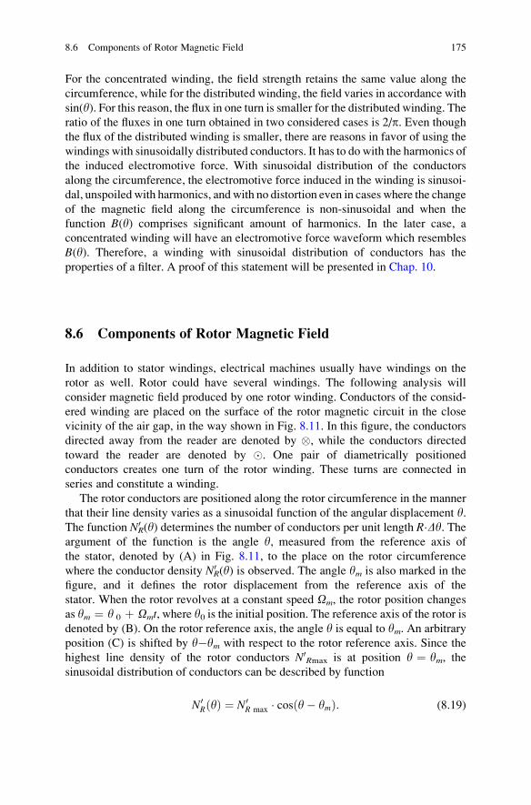
For the concentrated winding, the field strength retains the same value along the
circumference, while for the distributed winding, the field varies in accordance with
sin(y). For this reason, the flux in one turn is smaller for the distributed winding. The
ratio of the fluxes in one turn obtained in two considered cases is 2/p. Even though
the flux of the distributed winding is smaller, there are reasons in favor of using the
windings with sinusoidally distributed conductors. It has to do with the harmonics of
the induced electromotive force. With sinusoidal distribution of the conductors
along the circumference, the electromotive force induced in the winding is sinusoi-
dal, unspoiled with harmonics, andwith no distortion even in cases where the change
of the magnetic field along the circumference is non-sinusoidal and when the
function B(y) comprises significant amount of harmonics. In the later case, a
concentrated winding will have an electromotive force waveform which resembles
B(y). Therefore, a winding with sinusoidal distribution of conductors has the
properties of a filter. A proof of this statement will be presented in Chap. 10.
8.6 Components of Rotor Magnetic Field
In addition to stator windings, electrical machines usually have windings on the
rotor as well. Rotor could have several windings. The following analysis will
consider magnetic field produced by one rotor winding. Conductors of the consid-
ered winding are placed on the surface of the rotor magnetic circuit in the close
vicinity of the air gap, in the way shown in Fig. 8.11. In this figure, the conductors
directed away from the reader are denoted by �, while the conductors directed
toward the reader are denoted by �. One pair of diametrically positioned
conductors creates one turn of the rotor winding. These turns are connected in
series and constitute a winding.
The rotor conductors are positioned along the rotor circumference in the manner
that their line density varies as a sinusoidal function of the angular displacement y.The function NR
0 (y) determines the number of conductors per unit length R�Dy. Theargument of the function is the angle y, measured from the reference axis of
the stator, denoted by (A) in Fig. 8.11, to the place on the rotor circumference
where the conductor density NR0 (y) is observed. The angle ym is also marked in the
figure, and it defines the rotor displacement from the reference axis of the
stator. When the rotor revolves at a constant speed Om, the rotor position changes
as ym ¼ y 0 þ Omt, where y0 is the initial position. The reference axis of the rotor isdenoted by (B). On the rotor reference axis, the angle y is equal to ym. An arbitrary
position (C) is shifted by y�ym with respect to the rotor reference axis. Since the
highest line density of the rotor conductors N0Rmax is at position y ¼ ym, the
sinusoidal distribution of conductors can be described by function
N0R yð Þ ¼ N0
R max � cos y� ymð Þ: (8.19)
8.6 Components of Rotor Magnetic Field 175
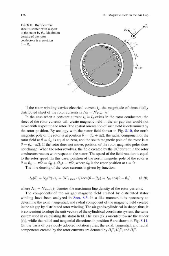
If the rotor winding carries electrical current i2, the magnitude of sinusoidally
distributed sheet of the rotor currents is JR0 ¼ N0Rmax i2.
In the case when a constant current i2 ¼ I2 exists in the rotor conductors, the
sheet of the rotor currents will create magnetic field in the air gap that would not
move with respect to the rotor. The spatial orientation of such field is determined by
the rotor position. By analogy with the stator field shown in Fig. 8.10, the north
magnetic pole of the rotor is at position y ¼ ym þ p/2, the radial component of the
rotor field at y ¼ ym is equal to zero, and the south magnetic pole of the rotor is at
y ¼ ym�p/2. If the rotor does not move, position of the rotor magnetic poles does
not change. When the rotor revolves, the field created by the DC current in the rotor
conductors rotates with respect to the stator. The speed of the field rotation is equal
to the rotor speed. In this case, position of the north magnetic pole of the rotor is
y ¼ ym þ p/2 ¼ y0 þ Omt þ p/2, where y0 is the rotor position at t ¼ 0.
The line density of the rotor currents is given by function
JR yð Þ ¼ N0R yð Þ � i2 ¼ N0
R max � i2ð Þ cos y� ymð Þ ¼ JR0 cos y� ymð Þ (8.20)
where JR0 ¼ N0Rmax i2 denotes the maximum line density of the rotor currents.
The components of the air gap magnetic field created by distributed stator
winding have been analyzed in Sect. 8.3. In a like manner, it is necessary to
determine the axial, tangential, and radial component of the magnetic field created
in the air gap by distributed rotor winding. The air gap is cylindrical in shape; thus, it
is convenient to adopt the unit vectors of the cylindrical coordinate system, the same
system used in calculating the stator field. The axis (z) is oriented toward the reader(�), while the radial and tangential directions in position y are shown in Fig. 8.11.
On the basis of previously adopted notation rules, the axial, tangential, and radial
components created by the rotor currents are denoted by HzR, Hy
R, and HrR.
Fig. 8.11 Rotor current
sheet is shifted with respect
to the stator by ym. Maximum
density of the rotor
conductors is at position
y ¼ ym
176 8 Magnetic Field in the Air Gap
Question (8.10): Conductors of the stator and rotor are placed in close vicinity of
the air gap. What are the negative effects of positioning the rotor conductors deeper
in the rotor magnetic circuit, further away from the air gap?
Answer (8.10): The lines of the magnetic field of a single conductor placed deeper
into the rotor magnetic circuit would close through the ferromagnetic material,
where magnetic resistance is lower, instead of passing through the air gap and
encircling the stator conductors. In cases where the rotor conductor is placed deep
into the iron magnetic circuit, far away from the air gap, the rotor magnetic field and
flux exist mainly in the rotor magnetic circuit and they do not extend neither to the
air gap nor to the stator winding. For this reason, there is significant reduction of
magnetic coupling between the rotor and stator windings. In such cases, most of the
rotor flux is the leakage flux, the part of the rotor flux which does not encircle
the stator windings. With the electromechanical conversion process being based on
the magnetic coupling, an increased rotor leakage greatly reduces the electromag-
netic torque and the conversion power. On the other hand, the rotor leakage is
reduced by placing the rotor conductors in rotor slots, next to the air gap. Magnetic
field of such conductors passes through the air gap and encircles conductors of the
stator, contributing to the magnetic coupling between stator and rotor windings.
8.6.1 Axial Component of the Rotor Field
It is proved in Sect. 8.3 that the axial component of the magnetic field is equal to
zero in cylindrical machines with axially placed conductors. Since electrical
currents exist in the conductors placed along z axis of the cylindrical coordinate
system, there are no currents in tangential direction. As a consequence, the axial
component of the magnetic field in the air gap is equal to zero. The analysis of
circulation of the field along the contour shown in Fig. 8.5 shows that the axial
component of the field in the air gap is equal to zero, notwithstanding the stator and
rotor currents.
8.6.2 Tangential Component of the Rotor Field
Tangential component of the rotor magnetic field HyR is calculated in the air gap,
next to the rotor magnetic circuit. The point of interest is in the air, and it resides on
the boundary surface separating the rotor magnetic circuit and the air gap.
The line integral of the magnetic field along the contour shown in Fig. 8.6 helps
calculating the magnetic field in the vicinity of the boundary surface between the
ferromagnetic material and the air gap. The tangential component of the field is
determined by the line density of the surface currents in the boundary plane.
Conclusions drawn from Fig. 8.6 can be applied to determining the tangential
8.6 Components of Rotor Magnetic Field 177
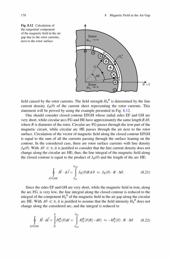
field caused by the rotor currents. The field strength HyR is determined by the line
current density JR(y) of the current sheet representing the rotor currents. This
statement will be proved by using the example presented in Fig. 8.12.
One should consider closed contour EFGH whose radial sides EF and GH are
very short, while circular arcs FG and HE have approximately the same length RDy,where R is diameter of the rotor. Circular arc FG passes through the iron part of the
magnetic circuit, while circular arc HE passes through the air next to the rotor
surface. Circulation of the vector of magnetic field along the closed contour EFGH
is equal to the sum of all the currents passing through the surface leaning on the
contour. In the considered case, there are rotor surface currents with line density
JR(y). With Dy � p, it is justified to consider that the line current density does not
change along the circular arc HE; thus, the line integral of the magnetic field along
the closed contour is equal to the product of JR(y) and the length of the arc HE:
þEFGHE
~H � d~l ¼ðyGH
yEF
JR yð ÞR d y � JR yð Þ � R � Dy: (8.21)
Since the sides EF and GH are very short, while the magnetic field in iron, along
the arc FG, is very low, the line integral along the closed contour is reduced to the
integral of the component HyR of the magnetic field in the air gap along the circular
arc HE. With Dy � p, it is justified to assume that the field intensity HyR does not
change along the considered arc, and the integral is reduced to
þEFGHE
~H � d~l ¼ðE
H
HRy yð Þdl ¼
ðyFEyGH
HRy yð ÞR �dyð Þ � �HR
y yð Þ � R � Dy (8.22)
Fig. 8.12 Calculation of
the tangential component
of the magnetic field in the air
gap due to the rotor currents,
next to the rotor surface
178 8 Magnetic Field in the Air Gap
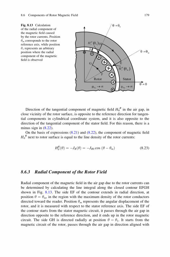
Direction of the tangential component of magnetic field HyR in the air gap, in
close vicinity of the rotor surface, is opposite to the reference direction for tangen-
tial components in cylindrical coordinate system, and it is also opposite to the
direction of the tangential component of the stator field. For this reason, there is a
minus sign in (8.22).
On the basis of expressions (8.21) and (8.22), the component of magnetic field
HyR next to rotor surface is equal to the line density of the rotor currents:
HRy yð Þ ¼ �JR yð Þ ¼ �JR0 cos y� ymð Þ (8.23)
8.6.3 Radial Component of the Rotor Field
Radial component of the magnetic field in the air gap due to the rotor currents can
be determined by calculating the line integral along the closed contour EFGH
shown in Fig. 8.13. The side EF of the contour extends in radial direction, at
position y ¼ ym, in the region with the maximum density of the rotor conductors
directed toward the reader. Position ym represents the angular displacement of the
rotor, and it is measured with respect to the stator reference axis. The side EF of
the contour starts from the stator magnetic circuit, it passes through the air gap in
direction opposite to the reference direction, and it ends up in the rotor magnetic
circuit. The side GH is directed radially at position y ¼ y1. It starts from the
magnetic circuit of the rotor, passes through the air gap in direction aligned with
Fig. 8.13 Calculation
of the radial component of
the magnetic field caused
by the rotor currents. Position
ym corresponds to the rotor
reference axis, while position
y1 represents an arbitrary
position where the radial
component of the magnetic
field is observed
8.6 Components of Rotor Magnetic Field 179
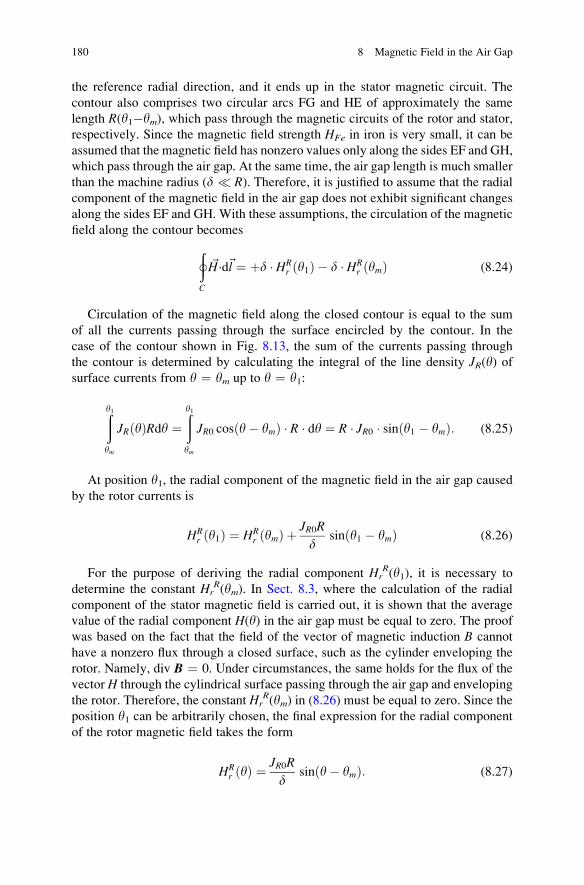
the reference radial direction, and it ends up in the stator magnetic circuit. The
contour also comprises two circular arcs FG and HE of approximately the same
length R(y1�ym), which pass through the magnetic circuits of the rotor and stator,
respectively. Since the magnetic field strength HFe in iron is very small, it can be
assumed that the magnetic field has nonzero values only along the sides EF and GH,
which pass through the air gap. At the same time, the air gap length is much smaller
than the machine radius (d � R). Therefore, it is justified to assume that the radial
component of the magnetic field in the air gap does not exhibit significant changes
along the sides EF and GH. With these assumptions, the circulation of the magnetic
field along the contour becomes
þC
~H�d~l ¼ þd � HRr ðy1Þ � d � HR
r ðymÞ (8.24)
Circulation of the magnetic field along the closed contour is equal to the sum
of all the currents passing through the surface encircled by the contour. In the
case of the contour shown in Fig. 8.13, the sum of the currents passing through
the contour is determined by calculating the integral of the line density JR(y) ofsurface currents from y ¼ ym up to y ¼ y1:
ðy1ym
JR yð ÞRdy ¼ðy1ym
JR0 cos y� ymð Þ � R � dy ¼ R � JR0 � sin y1 � ymð Þ: (8.25)
At position y1, the radial component of the magnetic field in the air gap caused
by the rotor currents is
HRr ðy1Þ ¼ HR
r ðymÞ þJR0R
dsinðy1 � ymÞ (8.26)
For the purpose of deriving the radial component HrR(y1), it is necessary to
determine the constant HrR(ym). In Sect. 8.3, where the calculation of the radial
component of the stator magnetic field is carried out, it is shown that the average
value of the radial component H(y) in the air gap must be equal to zero. The proof
was based on the fact that the field of the vector of magnetic induction B cannot
have a nonzero flux through a closed surface, such as the cylinder enveloping the
rotor. Namely, div B ¼ 0. Under circumstances, the same holds for the flux of the
vector H through the cylindrical surface passing through the air gap and enveloping
the rotor. Therefore, the constant HrR(ym) in (8.26) must be equal to zero. Since the
position y1 can be arbitrarily chosen, the final expression for the radial component
of the rotor magnetic field takes the form
HRr ðyÞ ¼
JR0R
dsinðy� ymÞ: (8.27)
180 8 Magnetic Field in the Air Gap
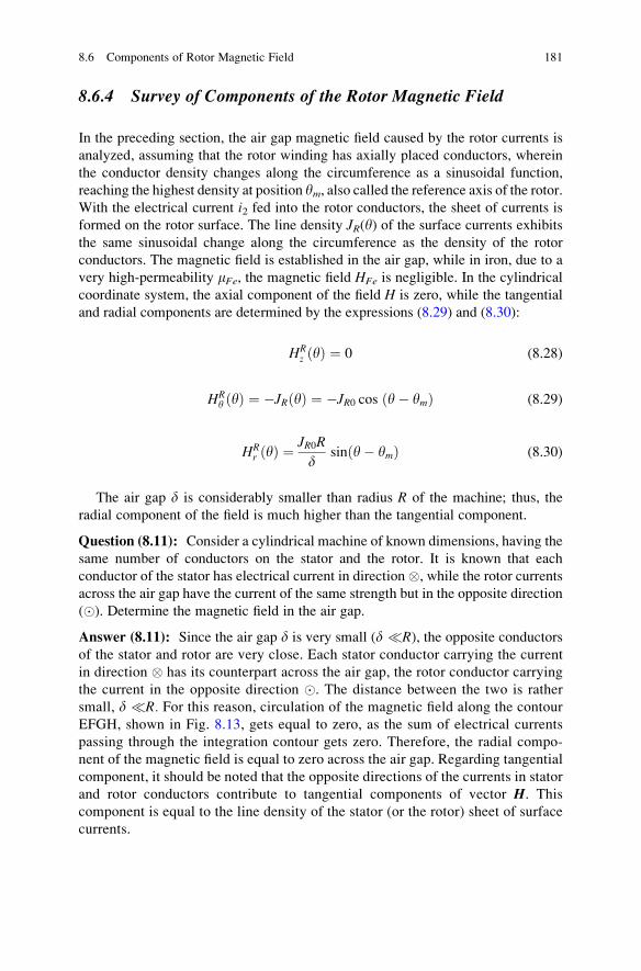
8.6.4 Survey of Components of the Rotor Magnetic Field
In the preceding section, the air gap magnetic field caused by the rotor currents is
analyzed, assuming that the rotor winding has axially placed conductors, wherein
the conductor density changes along the circumference as a sinusoidal function,
reaching the highest density at position ym, also called the reference axis of the rotor.With the electrical current i2 fed into the rotor conductors, the sheet of currents is
formed on the rotor surface. The line density JR(y) of the surface currents exhibitsthe same sinusoidal change along the circumference as the density of the rotor
conductors. The magnetic field is established in the air gap, while in iron, due to a
very high-permeability mFe, the magnetic field HFe is negligible. In the cylindrical
coordinate system, the axial component of the field H is zero, while the tangential
and radial components are determined by the expressions (8.29) and (8.30):
HRz ðyÞ ¼ 0 (8.28)
HRy yð Þ ¼ �JR yð Þ ¼ �JR0 cos y� ymð Þ (8.29)
HRr ðyÞ ¼
JR0R
dsinðy� ymÞ (8.30)
The air gap d is considerably smaller than radius R of the machine; thus, the
radial component of the field is much higher than the tangential component.
Question (8.11): Consider a cylindrical machine of known dimensions, having the
same number of conductors on the stator and the rotor. It is known that each
conductor of the stator has electrical current in direction �, while the rotor currents
across the air gap have the current of the same strength but in the opposite direction
(�). Determine the magnetic field in the air gap.
Answer (8.11): Since the air gap d is very small (d �R), the opposite conductorsof the stator and rotor are very close. Each stator conductor carrying the current
in direction � has its counterpart across the air gap, the rotor conductor carrying
the current in the opposite direction �. The distance between the two is rather
small, d �R. For this reason, circulation of the magnetic field along the contour
EFGH, shown in Fig. 8.13, gets equal to zero, as the sum of electrical currents
passing through the integration contour gets zero. Therefore, the radial compo-
nent of the magnetic field is equal to zero across the air gap. Regarding tangential
component, it should be noted that the opposite directions of the currents in stator
and rotor conductors contribute to tangential components of vector H. This
component is equal to the line density of the stator (or the rotor) sheet of surface
currents.
8.6 Components of Rotor Magnetic Field 181
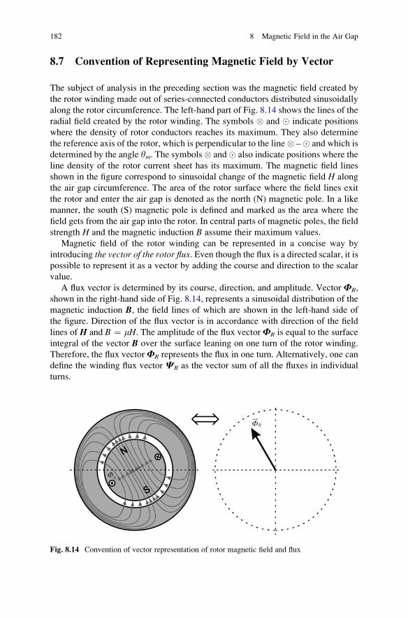
8.7 Convention of Representing Magnetic Field by Vector
The subject of analysis in the preceding section was the magnetic field created by
the rotor winding made out of series-connected conductors distributed sinusoidally
along the rotor circumference. The left-hand part of Fig. 8.14 shows the lines of the
radial field created by the rotor winding. The symbols � and � indicate positions
where the density of rotor conductors reaches its maximum. They also determine
the reference axis of the rotor, which is perpendicular to the line� –� and which is
determined by the angle ym. The symbols� and� also indicate positions where the
line density of the rotor current sheet has its maximum. The magnetic field lines
shown in the figure correspond to sinusoidal change of the magnetic field H along
the air gap circumference. The area of the rotor surface where the field lines exit
the rotor and enter the air gap is denoted as the north (N) magnetic pole. In a like
manner, the south (S) magnetic pole is defined and marked as the area where the
field gets from the air gap into the rotor. In central parts of magnetic poles, the field
strength H and the magnetic induction B assume their maximum values.
Magnetic field of the rotor winding can be represented in a concise way by
introducing the vector of the rotor flux. Even though the flux is a directed scalar, it ispossible to represent it as a vector by adding the course and direction to the scalar
value.
A flux vector is determined by its course, direction, and amplitude. Vector FR,
shown in the right-hand side of Fig. 8.14, represents a sinusoidal distribution of the
magnetic induction B, the field lines of which are shown in the left-hand side of
the figure. Direction of the flux vector is in accordance with direction of the field
lines of H and B ¼ mH. The amplitude of the flux vectorFR is equal to the surface
integral of the vector B over the surface leaning on one turn of the rotor winding.
Therefore, the flux vectorFR represents the flux in one turn. Alternatively, one can
define the winding flux vector CR as the vector sum of all the fluxes in individual
turns.
Fig. 8.14 Convention of vector representation of rotor magnetic field and flux
182 8 Magnetic Field in the Air Gap
Question (8.12): Behold the left side of Fig. 8.14 and the two rotor conductors
forming one rotor turn. Assume that these conductors are displaced several
millimeters toward the stator and positioned across the air gap, on the inner surface
of the stator magnetic circuit, while the electrical currents in these conductors
remain the same. In the prescribed way, what used to be a rotor turn becomes a
stator turn. Since the conductors denoted by � and � are now on the surface of the
stator magnetic circuit, the field created by the currents through these conductors
becomes now the stator field. Sketch the field lines and compare them with the lines
presented in the left-hand side of the figure. Denote positions of the north and south
magnetic poles of the stator flux created by these conductors.
Answer (8.12): Radial component of the magnetic field in the air gap will not
change by shifting the conductors. Direction of the tangential component of the
field will change. Since radial component prevails over tangential component by an
order of magnitude, it can be concluded that shifting the conductors will have no
influence on the shape of the field lines. It is of interest to note that the north pole
corresponds to the region where the magnetic field is directed from the magnetic
circuit toward the air gap. In Fig. 8.14, the north pole of the stator is opposite to the
south pole of the rotor.
8.7 Convention of Representing Magnetic Field by Vector 183
Chapter 9
Energy, Flux, and Torque
Magnetic field in the air gap is obtained from electrical currents in stator and rotor
windings. Another source of the air gap field can be permanent magnets that may be
placed within magnetic circuits of either stator or rotor. The stator and rotor fields in
the air gap are calculated in the previous chapter. Interaction of the two fields incites
the process of electromechanical conversion.
In this chapter, expressions for the magnetic field in the air gap are used to
calculate the field energy, to derive the energy accumulated in the magnetic field,
and to calculate the electromagnetic torque caused by the interaction between the
stator and rotor fields. In order to simplify the analysis, the flux linkages in one turns
and the winding fluxes are represented by flux vectors. The concept of flux vector isintroduced and explained along with magnetic axes of turns and windings. The
torque expression is rewritten and expressed as the vector product of stator and rotorflux vectors. It is pointed out that continuous torque generation requires either statoror rotor windings to create the revolving magnetic field. This chapter ends with the
analysis of two-phase windings systems and three-phase winding systems that
create revolving magnetic field.
9.1 Interaction of the Stator and Rotor Fields
Electrical machines usually have windings on both stator and rotor. Currents
through the windings create stator and rotor fluxes. There are machines which
have permanent magnets instead of the stator or rotor winding. Magnetic field in
the air gap has its radial and tangential components. The radial component is R/dtimes larger than the tangential. It determines the spatial distribution of the mag-
netic energy of the field, as well as the course and direction of the field lines.
The stator and rotor fields exist in the same air gap and the same magnetic
circuit. They add up and make the resulting magnetic field and the resulting flux.
Assuming that magnetic circuit is linear (m ¼ const.), the resulting field is obtained
by superposition of stator and rotor fields. Namely, the strength of the resulting
S.N. Vukosavic, Electrical Machines, Power Electronics and Power Systems,
DOI 10.1007/978-1-4614-0400-2_9, # Springer Science+Business Media New York 2013
185
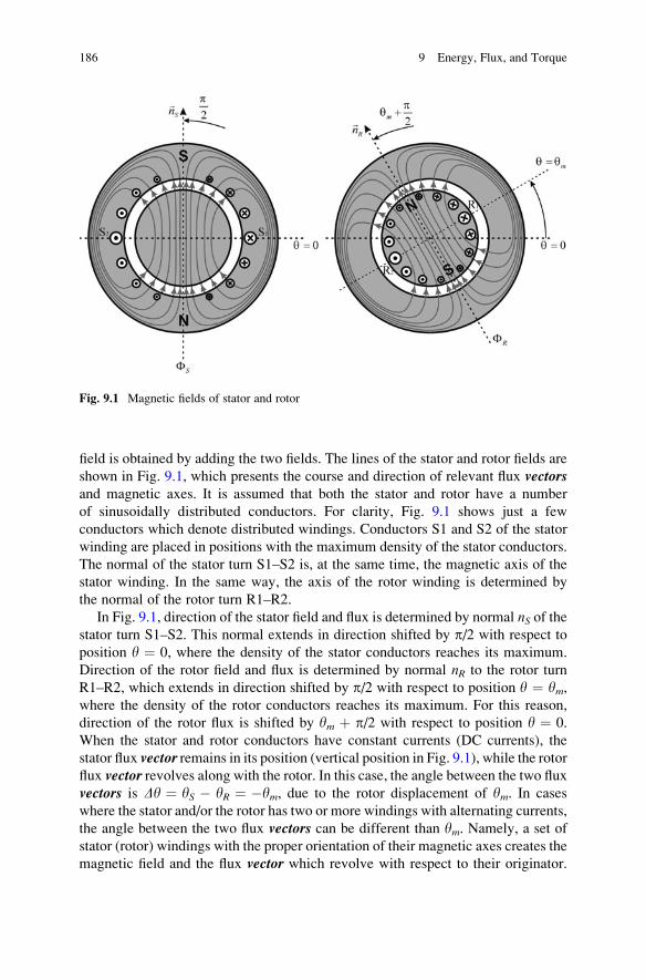
field is obtained by adding the two fields. The lines of the stator and rotor fields are
shown in Fig. 9.1, which presents the course and direction of relevant flux vectorsand magnetic axes. It is assumed that both the stator and rotor have a number
of sinusoidally distributed conductors. For clarity, Fig. 9.1 shows just a few
conductors which denote distributed windings. Conductors S1 and S2 of the stator
winding are placed in positions with the maximum density of the stator conductors.
The normal of the stator turn S1–S2 is, at the same time, the magnetic axis of the
stator winding. In the same way, the axis of the rotor winding is determined by
the normal of the rotor turn R1–R2.
In Fig. 9.1, direction of the stator field and flux is determined by normal nS of thestator turn S1–S2. This normal extends in direction shifted by p/2 with respect to
position y ¼ 0, where the density of the stator conductors reaches its maximum.
Direction of the rotor field and flux is determined by normal nR to the rotor turn
R1–R2, which extends in direction shifted by p/2 with respect to position y ¼ ym,where the density of the rotor conductors reaches its maximum. For this reason,
direction of the rotor flux is shifted by ym þ p/2 with respect to position y ¼ 0.
When the stator and rotor conductors have constant currents (DC currents), the
stator flux vector remains in its position (vertical position in Fig. 9.1), while the rotor
flux vector revolves along with the rotor. In this case, the angle between the two fluxvectors is Dy ¼ yS � yR ¼ �ym, due to the rotor displacement of ym. In cases
where the stator and/or the rotor has two or more windings with alternating currents,
the angle between the two flux vectors can be different than ym. Namely, a set of
stator (rotor) windings with the proper orientation of their magnetic axes creates the
magnetic field and the flux vector which revolve with respect to their originator.
Fig. 9.1 Magnetic fields of stator and rotor
186 9 Energy, Flux, and Torque
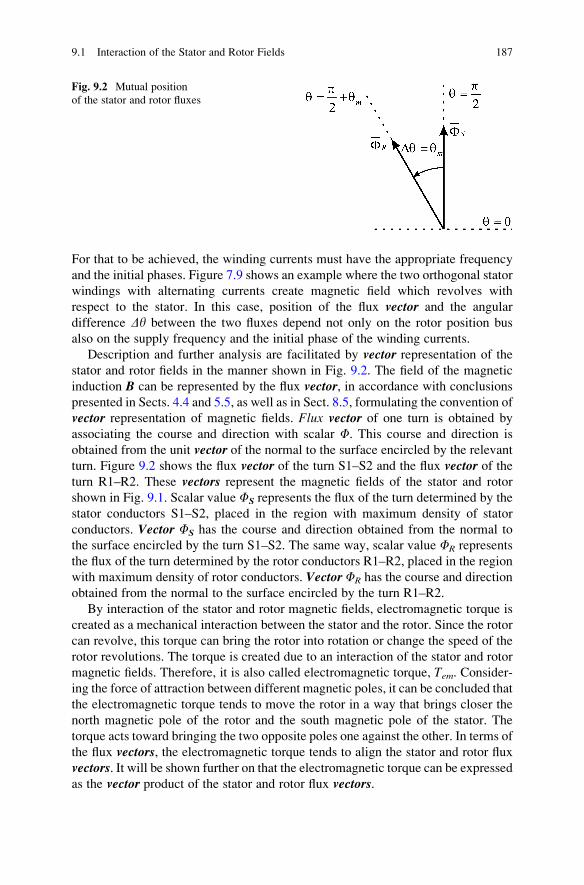
For that to be achieved, the winding currents must have the appropriate frequency
and the initial phases. Figure 7.9 shows an example where the two orthogonal stator
windings with alternating currents create magnetic field which revolves with
respect to the stator. In this case, position of the flux vector and the angular
difference Dy between the two fluxes depend not only on the rotor position bus
also on the supply frequency and the initial phase of the winding currents.
Description and further analysis are facilitated by vector representation of the
stator and rotor fields in the manner shown in Fig. 9.2. The field of the magnetic
induction B can be represented by the flux vector, in accordance with conclusions
presented in Sects. 4.4 and 5.5, as well as in Sect. 8.5, formulating the convention of
vector representation of magnetic fields. Flux vector of one turn is obtained by
associating the course and direction with scalar F. This course and direction is
obtained from the unit vector of the normal to the surface encircled by the relevant
turn. Figure 9.2 shows the flux vector of the turn S1–S2 and the flux vector of theturn R1–R2. These vectors represent the magnetic fields of the stator and rotor
shown in Fig. 9.1. Scalar value FS represents the flux of the turn determined by the
stator conductors S1–S2, placed in the region with maximum density of stator
conductors. Vector FS has the course and direction obtained from the normal to
the surface encircled by the turn S1–S2. The same way, scalar value FR represents
the flux of the turn determined by the rotor conductors R1–R2, placed in the region
with maximum density of rotor conductors. Vector FR has the course and direction
obtained from the normal to the surface encircled by the turn R1–R2.
By interaction of the stator and rotor magnetic fields, electromagnetic torque is
created as a mechanical interaction between the stator and the rotor. Since the rotor
can revolve, this torque can bring the rotor into rotation or change the speed of the
rotor revolutions. The torque is created due to an interaction of the stator and rotor
magnetic fields. Therefore, it is also called electromagnetic torque, Tem. Consider-ing the force of attraction between different magnetic poles, it can be concluded that
the electromagnetic torque tends to move the rotor in a way that brings closer the
north magnetic pole of the rotor and the south magnetic pole of the stator. The
torque acts toward bringing the two opposite poles one against the other. In terms of
the flux vectors, the electromagnetic torque tends to align the stator and rotor flux
vectors. It will be shown further on that the electromagnetic torque can be expressed
as the vector product of the stator and rotor flux vectors.
Fig. 9.2 Mutual position
of the stator and rotor fluxes
9.1 Interaction of the Stator and Rotor Fields 187
Question (9.1): Assume that stator magnetic poles do not move with respect to the
stator. In addition, assume that rotor magnetic poles do not move with respect to
the rotor. If the rotor revolves at a constant speed, what is the change of the torque
acting on the rotor?
Answer (9.1): In the considered case, the angle Dy between the flux vectors of thestator and rotor is equal to the shift ym. If the rotor revolves at a constant speed,
the variation of the created electromagnetic torque will be sinusoidal.
9.2 Energy of Air Gap Magnetic Field
It is of interest to determine the electromagnetic torque acting on the rotor and stator
of a cylindrical machine. This torque can be determined as the first derivative of the
energy accumulated in the magnetic (coupling) field in terms of the rotor displace-
ment ym. On the basis of the equations given in Sect. 6.9, the increment of mechani-
cal work dWmeh ¼ Temdym is equal to the increment of energy of the magnetic field;
thus, the torque can be determined as the first derivative of the magnetic field energy
in terms of the rotor shift ym, dWm/dym. Therefore, it is necessary to determine the
energy of the magnetic field in terms of the rotor position, Wm(ym).The energy of the magnetic field can be calculated by integrating the density of
the field energy wm over the entire domain where the magnetic field exists. The
energy density wm is expressed in J/m3, and it represents the amount of the field
energy comprised within unit volume; thus, wm ¼ DWm/DV ¼ dWm/dV. Expres-sion wm ¼ ½ mH2 determines the density of the field energy in a linear medium,
where the magnetic permeability does not change. Therefore, the density of the
field energy in the air gap is wm ¼ ½m0H2.
Magnetic field exists in the magnetic circuits of the stator and rotor which are
made of iron, as well as in the air gap. Since the same magnetic flux which passes
through the air gap gets into the stator and rotor magnetic circuits, magnetic
induction in iron BFe and in the air gap B0 is roughly the same. The permeability
of iron mFe is several orders of magnitude higher than the permeability of the air m0.Therefore, the magnetic field in iron HFe ¼ BFe/mFe is negligible compared to the
fieldH0 in the air gap. The sameway, the density of the field energy in iron (½B2/mFe)is negligible when compared to the density of the field energy in the air gap (½B2/m0).For this reason, the overall energy of the magnetic field can be determined by
integrating the density of the field energy (specific energy) over the whole domain
of the air gap.
In the expression for the field energy density wm ¼ ½m0H2, the symbol H
represents the strength of the resultant magnetic field in the air gap, namely, the
sum of the stator and rotor fields. Since the tangential components of the magnetic
field are negligible (d � R), the strength H of the resulting magnetic field in the air
gap is equal to the sum of radial components of the stator and rotor fields.
188 9 Energy, Flux, and Torque
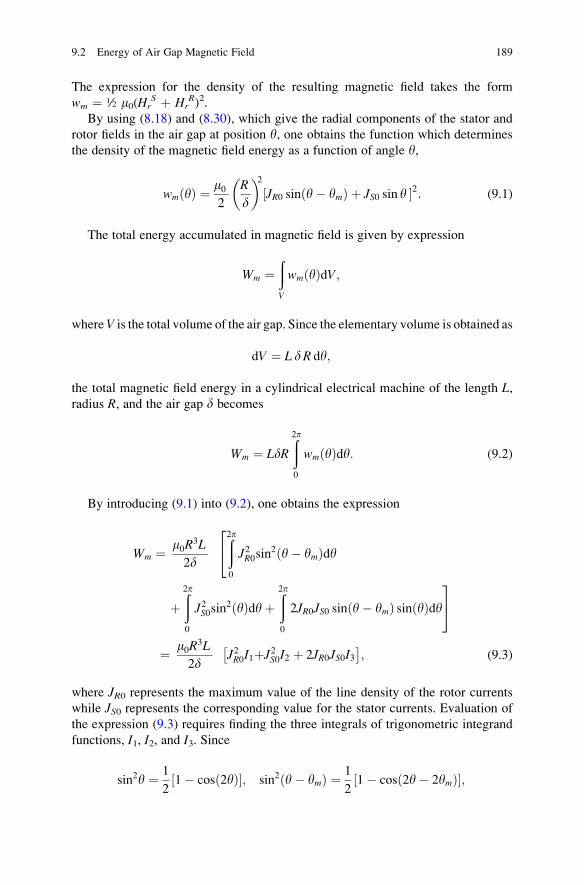
The expression for the density of the resulting magnetic field takes the form
wm ¼ ½ m0(HrS þ Hr
R)2.
By using (8.18) and (8.30), which give the radial components of the stator and
rotor fields in the air gap at position y, one obtains the function which determines
the density of the magnetic field energy as a function of angle y,
wm yð Þ ¼ m02
R
d
� �2JR0 sin y� ymð Þ þ JS0 sin y½ �2: (9.1)
The total energy accumulated in magnetic field is given by expression
Wm ¼ðV
wmðyÞdV;
whereV is the total volume of the air gap. Since the elementary volume is obtained as
dV ¼ L dR dy;
the total magnetic field energy in a cylindrical electrical machine of the length L,radius R, and the air gap d becomes
Wm ¼ LdRð2p
0
wm yð Þdy: (9.2)
By introducing (9.1) into (9.2), one obtains the expression
Wm ¼ m0R3L
2d
ð2p
0
J2R0sin2 y� ymð Þdy
24
þð2p
0
J2S0sin2 yð Þdyþ
ð2p
0
2JR0JS0 sin y� ymð Þ sin yð Þdy35
¼ m0R3L
2dJ2R0I1� þJ2S0I2 þ 2JR0JS0I3
�; (9.3)
where JR0 represents the maximum value of the line density of the rotor currents
while JS0 represents the corresponding value for the stator currents. Evaluation of
the expression (9.3) requires finding the three integrals of trigonometric integrand
functions, I1, I2, and I3. Since
sin2y ¼ 1
21� cos 2yð Þ½ �; sin2 y� ymð Þ ¼ 1
21� cos 2y� 2ymð Þ½ �;
9.2 Energy of Air Gap Magnetic Field 189
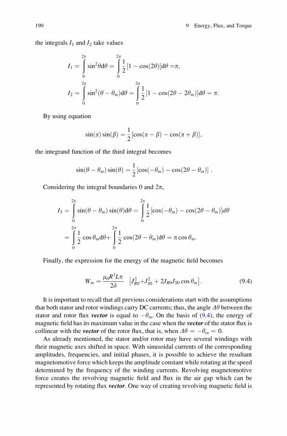
the integrals I1 and I2 take values
I1 ¼ð2p
0
sin2ydy ¼ð2p
0
1
21� cos 2yð Þ½ �dy ¼p;
I2 ¼ð2p
0
sin2 y� ymð Þdy ¼ð2p
0
1
21� cos 2y� 2ymð Þ½ �dy ¼ p:
By using equation
sin að Þ sin bð Þ ¼ 1
2cos a� bð Þ � cos aþ bð Þ½ �;
the integrand function of the third integral becomes
sin y� ymð Þ sin yð Þ ¼ 1
2cos �ymð Þ � cos 2y� ymð Þ½ � :
Considering the integral boundaries 0 and 2p,
I3 ¼ð2p
0
sin y� ymð Þ sin yð Þdy ¼ð2p
0
1
2cos �ymð Þ � cos 2y� ymð Þ½ �dy
¼ð2p
0
1
2cos ymdyþ
ð2p
0
1
2cos 2y� ymð Þdy ¼ p cos ym:
Finally, the expression for the energy of the magnetic field becomes
Wm ¼ m0R3Lp2d
J2R0� þJ2S0 þ 2JR0JS0 cos ym
�: (9.4)
It is important to recall that all previous considerations start with the assumptions
that both stator and rotor windings carry DC currents; thus, the angleDy between thestator and rotor flux vector is equal to �ym. On the basis of (9.4), the energy of
magnetic field has its maximum value in the case when the vector of the stator flux iscollinear with the vector of the rotor flux, that is, when Dy ¼ �ym ¼ 0.
As already mentioned, the stator and/or rotor may have several windings with
their magnetic axes shifted in space. With sinusoidal currents of the corresponding
amplitudes, frequencies, and initial phases, it is possible to achieve the resultant
magnetomotive force which keeps the amplitude constant while rotating at the speed
determined by the frequency of the winding currents. Revolving magnetomotive
force creates the revolving magnetic field and flux in the air gap which can be
represented by rotating flux vector. One way of creating revolving magnetic field is
190 9 Energy, Flux, and Torque
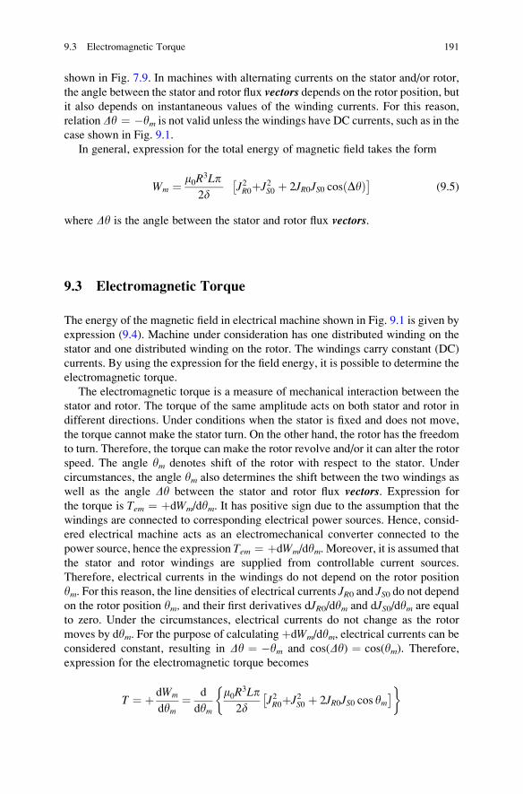
shown in Fig. 7.9. In machines with alternating currents on the stator and/or rotor,
the angle between the stator and rotor flux vectors depends on the rotor position, butit also depends on instantaneous values of the winding currents. For this reason,
relation Dy ¼ �ym is not valid unless the windings have DC currents, such as in the
case shown in Fig. 9.1.
In general, expression for the total energy of magnetic field takes the form
Wm ¼ m0R3Lp2d
J2R0� þJ2S0 þ 2JR0JS0 cos Dyð Þ� (9.5)
where Dy is the angle between the stator and rotor flux vectors.
9.3 Electromagnetic Torque
The energy of the magnetic field in electrical machine shown in Fig. 9.1 is given by
expression (9.4). Machine under consideration has one distributed winding on the
stator and one distributed winding on the rotor. The windings carry constant (DC)
currents. By using the expression for the field energy, it is possible to determine the
electromagnetic torque.
The electromagnetic torque is a measure of mechanical interaction between the
stator and rotor. The torque of the same amplitude acts on both stator and rotor in
different directions. Under conditions when the stator is fixed and does not move,
the torque cannot make the stator turn. On the other hand, the rotor has the freedom
to turn. Therefore, the torque can make the rotor revolve and/or it can alter the rotor
speed. The angle ym denotes shift of the rotor with respect to the stator. Under
circumstances, the angle ym also determines the shift between the two windings as
well as the angle Dy between the stator and rotor flux vectors. Expression for
the torque is Tem ¼ þdWm/dym. It has positive sign due to the assumption that the
windings are connected to corresponding electrical power sources. Hence, consid-
ered electrical machine acts as an electromechanical converter connected to the
power source, hence the expression Tem ¼ þdWm/dym. Moreover, it is assumed that
the stator and rotor windings are supplied from controllable current sources.
Therefore, electrical currents in the windings do not depend on the rotor position
ym. For this reason, the line densities of electrical currents JR0 and JS0 do not dependon the rotor position ym, and their first derivatives dJR0/dym and dJS0/dym are equal
to zero. Under the circumstances, electrical currents do not change as the rotor
moves by dym. For the purpose of calculating þdWm/dym, electrical currents can beconsidered constant, resulting in Dy ¼ �ym and cos(Dy) ¼ cos(ym). Therefore,expression for the electromagnetic torque becomes
T ¼ þ dWm
dym¼ d
dym
m0R3Lp
2dJ2R0� þJ2S0 þ 2JR0JS0 cos ym
�� �
9.3 Electromagnetic Torque 191
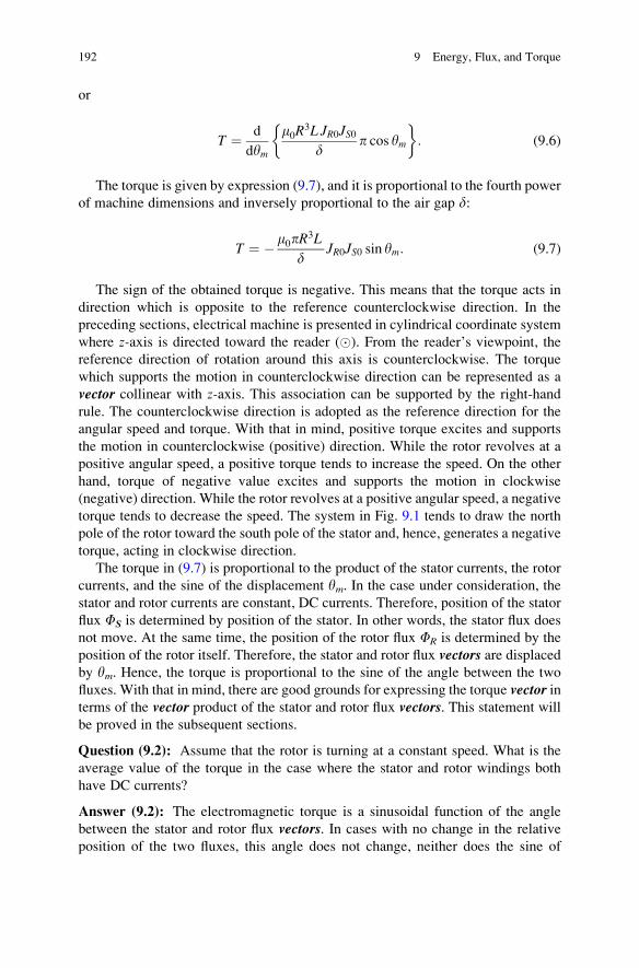
or
T ¼ d
dym
m0R3L JR0JS0d
p cos ym
� �: (9.6)
The torque is given by expression (9.7), and it is proportional to the fourth power
of machine dimensions and inversely proportional to the air gap d:
T ¼ � m0pR3L
dJR0JS0 sin ym: (9.7)
The sign of the obtained torque is negative. This means that the torque acts in
direction which is opposite to the reference counterclockwise direction. In the
preceding sections, electrical machine is presented in cylindrical coordinate system
where z-axis is directed toward the reader (�). From the reader’s viewpoint, the
reference direction of rotation around this axis is counterclockwise. The torque
which supports the motion in counterclockwise direction can be represented as a
vector collinear with z-axis. This association can be supported by the right-hand
rule. The counterclockwise direction is adopted as the reference direction for the
angular speed and torque. With that in mind, positive torque excites and supports
the motion in counterclockwise (positive) direction. While the rotor revolves at a
positive angular speed, a positive torque tends to increase the speed. On the other
hand, torque of negative value excites and supports the motion in clockwise
(negative) direction. While the rotor revolves at a positive angular speed, a negative
torque tends to decrease the speed. The system in Fig. 9.1 tends to draw the north
pole of the rotor toward the south pole of the stator and, hence, generates a negative
torque, acting in clockwise direction.
The torque in (9.7) is proportional to the product of the stator currents, the rotor
currents, and the sine of the displacement ym. In the case under consideration, the
stator and rotor currents are constant, DC currents. Therefore, position of the stator
flux FS is determined by position of the stator. In other words, the stator flux does
not move. At the same time, the position of the rotor flux FR is determined by the
position of the rotor itself. Therefore, the stator and rotor flux vectors are displacedby ym. Hence, the torque is proportional to the sine of the angle between the two
fluxes. With that in mind, there are good grounds for expressing the torque vector interms of the vector product of the stator and rotor flux vectors. This statement will
be proved in the subsequent sections.
Question (9.2): Assume that the rotor is turning at a constant speed. What is the
average value of the torque in the case where the stator and rotor windings both
have DC currents?
Answer (9.2): The electromagnetic torque is a sinusoidal function of the angle
between the stator and rotor flux vectors. In cases with no change in the relative
position of the two fluxes, this angle does not change, neither does the sine of
192 9 Energy, Flux, and Torque
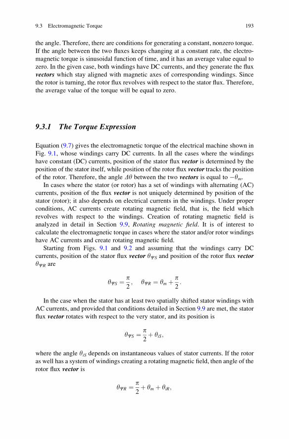
the angle. Therefore, there are conditions for generating a constant, nonzero torque.
If the angle between the two fluxes keeps changing at a constant rate, the electro-
magnetic torque is sinusoidal function of time, and it has an average value equal to
zero. In the given case, both windings have DC currents, and they generate the flux
vectors which stay aligned with magnetic axes of corresponding windings. Since
the rotor is turning, the rotor flux revolves with respect to the stator flux. Therefore,
the average value of the torque will be equal to zero.
9.3.1 The Torque Expression
Equation (9.7) gives the electromagnetic torque of the electrical machine shown in
Fig. 9.1, whose windings carry DC currents. In all the cases where the windings
have constant (DC) currents, position of the stator flux vector is determined by the
position of the stator itself, while position of the rotor flux vector tracks the positionof the rotor. Therefore, the angle Dy between the two vectors is equal to �ym.
In cases where the stator (or rotor) has a set of windings with alternating (AC)
currents, position of the flux vector is not uniquely determined by position of the
stator (rotor); it also depends on electrical currents in the windings. Under proper
conditions, AC currents create rotating magnetic field, that is, the field which
revolves with respect to the windings. Creation of rotating magnetic field is
analyzed in detail in Section 9.9, Rotating magnetic field. It is of interest to
calculate the electromagnetic torque in cases where the stator and/or rotor windings
have AC currents and create rotating magnetic field.
Starting from Figs. 9.1 and 9.2 and assuming that the windings carry DC
currents, position of the stator flux vector yCS and position of the rotor flux vectoryCR are
yCS ¼ p2; yCR ¼ ym þ p
2:
In the case when the stator has at least two spatially shifted stator windings with
AC currents, and provided that conditions detailed in Section 9.9 are met, the stator
flux vector rotates with respect to the very stator, and its position is
yCS ¼ p2þ yiS;
where the angle yiS depends on instantaneous values of stator currents. If the rotor
as well has a system of windings creating a rotating magnetic field, then angle of the
rotor flux vector is
yCR ¼ p2þ ym þ yiR;
9.3 Electromagnetic Torque 193
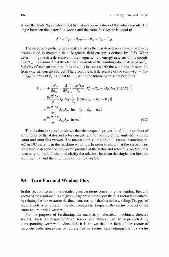
where the angle yiR is determined by instantaneous values of the rotor currents. The
angle between the stator flux vector and the rotor flux vector is equal to
Dy ¼ yCS � yCR ¼ �ym þ yiS � yiR:
The electromagnetic torque is calculated as the first derivative (9.8) of the energy
accumulated in magnetic field. Magnetic field energy is defined by (9.5). When
determining the first derivative of the magnetic field energy in terms of the coordi-
nate ym, it is assumed that the electrical currents in the windings do not depend on ym.Validity of such an assumption is obvious in cases where the windings are supplied
from external current sources. Therefore, the first derivative of the sum�ym þ yCS
þ yCR in terms of ym is equal to �1, while the torque expression becomes
Tem ¼ þ dWm
dym¼ d
dym
m0R3Lp
2dJ2R0� þJ2S0 þ 2JR0JS0 cos Dyð Þ�
� �
¼ m0R3Lpd
JR0JS0d
dymcos �ym þ yiS � yiRð Þ½ �
¼ m0R3Lpd
JR0JS0 sin �ym þ yiS � yiRð Þ
¼ m0R3Lpd
JR0JS0 sinDy: (9.8)
The obtained expression shows that the torque is proportional to the product of
amplitudes of the stator and rotor currents and to the sine of the angle between the
stator and rotor flux vectors. The torque expression (9.8) holds notwithstanding the
AC or DC currents in the machine windings. In order to show that the electromag-
netic torque depends on the vector product of the stator and rotor flux vectors, it isnecessary to probe further and clarify the relations between the single turn flux, the
winding flux, and the amplitude of the flux vector.
9.4 Turn Flux and Winding Flux
In this section, some more detailed considerations concerning the winding flux and
vector of the resultant flux are given.Algebraic intensity of the flux vector is calculatedby relating the flux vector to the flux in one turn and the flux in thewinding. The goal ofthese efforts is to represent the electromagnetic torque as the vector product of thestator and rotor flux vectors.
For the purpose of facilitating the analysis of electrical machines, directed
scalars, such as magnetomotive forces and fluxes, can be represented by
corresponding vectors. In Sect. 4.4, it is shown that the field of the vector of
magnetic induction B can be represented by vector, thus defining the flux vector
194 9 Energy, Flux, and Torque
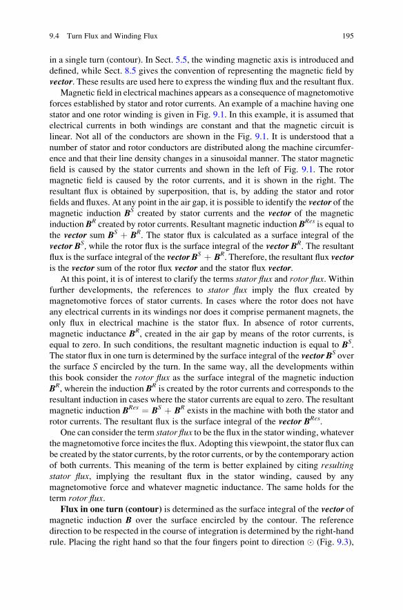
in a single turn (contour). In Sect. 5.5, the winding magnetic axis is introduced and
defined, while Sect. 8.5 gives the convention of representing the magnetic field by
vector. These results are used here to express the winding flux and the resultant flux.Magnetic field in electrical machines appears as a consequence of magnetomotive
forces established by stator and rotor currents. An example of a machine having one
stator and one rotor winding is given in Fig. 9.1. In this example, it is assumed that
electrical currents in both windings are constant and that the magnetic circuit is
linear. Not all of the conductors are shown in the Fig. 9.1. It is understood that a
number of stator and rotor conductors are distributed along the machine circumfer-
ence and that their line density changes in a sinusoidal manner. The stator magnetic
field is caused by the stator currents and shown in the left of Fig. 9.1. The rotor
magnetic field is caused by the rotor currents, and it is shown in the right. The
resultant flux is obtained by superposition, that is, by adding the stator and rotor
fields and fluxes. At any point in the air gap, it is possible to identify the vector of themagnetic induction BS created by stator currents and the vector of the magnetic
induction BR created by rotor currents. Resultant magnetic induction BRes is equal to
the vector sum BS þ BR. The stator flux is calculated as a surface integral of the
vector BS, while the rotor flux is the surface integral of the vector BR. The resultant
flux is the surface integral of the vector BS þ BR. Therefore, the resultant flux vectoris the vector sum of the rotor flux vector and the stator flux vector.
At this point, it is of interest to clarify the terms stator flux and rotor flux. Within
further developments, the references to stator flux imply the flux created by
magnetomotive forces of stator currents. In cases where the rotor does not have
any electrical currents in its windings nor does it comprise permanent magnets, the
only flux in electrical machine is the stator flux. In absence of rotor currents,
magnetic inductance BR, created in the air gap by means of the rotor currents, is
equal to zero. In such conditions, the resultant magnetic induction is equal to BS.
The stator flux in one turn is determined by the surface integral of the vector BS over
the surface S encircled by the turn. In the same way, all the developments within
this book consider the rotor flux as the surface integral of the magnetic induction
BR, wherein the induction BR is created by the rotor currents and corresponds to the
resultant induction in cases where the stator currents are equal to zero. The resultant
magnetic induction BRes ¼ BS þ BR exists in the machine with both the stator and
rotor currents. The resultant flux is the surface integral of the vector BRes.
One can consider the term stator flux to be the flux in the stator winding, whateverthe magnetomotive force incites the flux. Adopting this viewpoint, the stator flux can
be created by the stator currents, by the rotor currents, or by the contemporary action
of both currents. This meaning of the term is better explained by citing resultingstator flux, implying the resultant flux in the stator winding, caused by any
magnetomotive force and whatever magnetic inductance. The same holds for the
term rotor flux.Flux in one turn (contour) is determined as the surface integral of the vector of
magnetic induction B over the surface encircled by the contour. The reference
direction to be respected in the course of integration is determined by the right-hand
rule. Placing the right hand so that the four fingers point to direction � (Fig. 9.3),
9.4 Turn Flux and Winding Flux 195
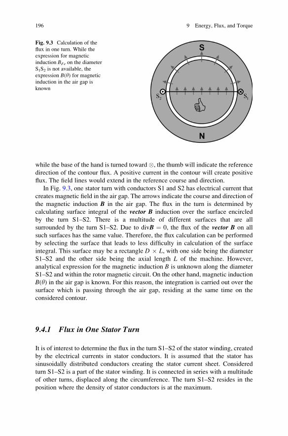
while the base of the hand is turned toward �, the thumb will indicate the reference
direction of the contour flux. A positive current in the contour will create positive
flux. The field lines would extend in the reference course and direction.
In Fig. 9.3, one stator turn with conductors S1 and S2 has electrical current that
creates magnetic field in the air gap. The arrows indicate the course and direction of
the magnetic induction B in the air gap. The flux in the turn is determined by
calculating surface integral of the vector B induction over the surface encircled
by the turn S1–S2. There is a multitude of different surfaces that are all
surrounded by the turn S1–S2. Due to divB ¼ 0, the flux of the vector B on all
such surfaces has the same value. Therefore, the flux calculation can be performed
by selecting the surface that leads to less difficulty in calculation of the surface
integral. This surface may be a rectangle D � L, with one side being the diameter
S1–S2 and the other side being the axial length L of the machine. However,
analytical expression for the magnetic induction B is unknown along the diameter
S1–S2 and within the rotor magnetic circuit. On the other hand, magnetic induction
B(y) in the air gap is known. For this reason, the integration is carried out over the
surface which is passing through the air gap, residing at the same time on the
considered contour.
9.4.1 Flux in One Stator Turn
It is of interest to determine the flux in the turn S1–S2 of the stator winding, created
by the electrical currents in stator conductors. It is assumed that the stator has
sinusoidally distributed conductors creating the stator current sheet. Considered
turn S1–S2 is a part of the stator winding. It is connected in series with a multitude
of other turns, displaced along the circumference. The turn S1–S2 resides in the
position where the density of stator conductors is at the maximum.
Fig. 9.3 Calculation of the
flux in one turn. While the
expression for magnetic
induction BFe on the diameter
S1S2 is not available, the
expression B(y) for magnetic
induction in the air gap is
known
196 9 Energy, Flux, and Torque
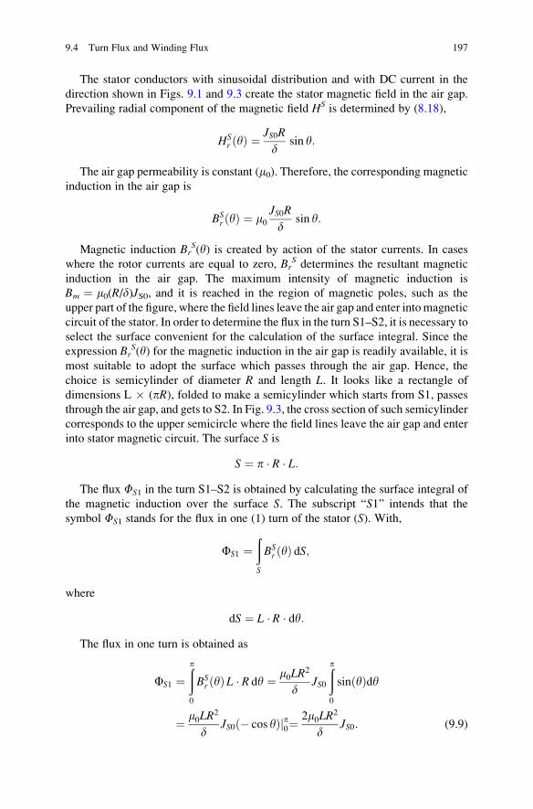
The stator conductors with sinusoidal distribution and with DC current in the
direction shown in Figs. 9.1 and 9.3 create the stator magnetic field in the air gap.
Prevailing radial component of the magnetic field HS is determined by (8.18),
HSr ðyÞ ¼
JS0R
dsin y:
The air gap permeability is constant (m0). Therefore, the corresponding magnetic
induction in the air gap is
BSr ðyÞ ¼ m0
JS0R
dsin y:
Magnetic induction BrS(y) is created by action of the stator currents. In cases
where the rotor currents are equal to zero, BrS determines the resultant magnetic
induction in the air gap. The maximum intensity of magnetic induction is
Bm ¼ m0(R/d)JS0, and it is reached in the region of magnetic poles, such as the
upper part of the figure, where the field lines leave the air gap and enter intomagnetic
circuit of the stator. In order to determine the flux in the turn S1–S2, it is necessary to
select the surface convenient for the calculation of the surface integral. Since the
expression BrS(y) for the magnetic induction in the air gap is readily available, it is
most suitable to adopt the surface which passes through the air gap. Hence, the
choice is semicylinder of diameter R and length L. It looks like a rectangle of
dimensions L � (pR), folded to make a semicylinder which starts from S1, passes
through the air gap, and gets to S2. In Fig. 9.3, the cross section of such semicylinder
corresponds to the upper semicircle where the field lines leave the air gap and enter
into stator magnetic circuit. The surface S is
S ¼ p � R � L:The flux FS1 in the turn S1–S2 is obtained by calculating the surface integral of
the magnetic induction over the surface S. The subscript “S1” intends that the
symbol FS1 stands for the flux in one (1) turn of the stator (S). With,
FS1 ¼ðS
BSr yð Þ dS;
where
dS ¼ L � R � dy:The flux in one turn is obtained as
FS1 ¼ðp
0
BSr yð Þ L � R dy ¼ m0LR
2
dJS0
ðp
0
sin yð Þdy
¼ m0LR2
dJS0 � cos yð Þjp0¼
2m0LR2
dJS0: (9.9)
9.4 Turn Flux and Winding Flux 197
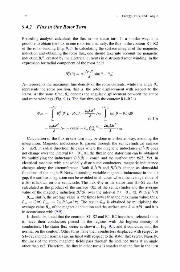
9.4.2 Flux in One Rotor Turn
Preceding analysis calculates the flux in one stator turn. In a similar way, it is
possible to obtain the flux in one rotor turn, namely, the flux in the contour R1–R2
of the rotor winding (Fig. 9.1). In calculating the surface integral of the magnetic
induction and obtaining the rotor flux, one should take into account the magnetic
induction BrR, created by the electrical currents in distributed rotor winding. In the
expression for radial component of the rotor field
BRr ðyÞ ¼ m0
JR0R
dsin y� ymð Þ:
JR0 represents the maximum line density of the rotor currents, while the angle ymrepresents the rotor position, that is, the rotor displacement with respect to the
stator. At the same time, ym denotes the angular displacement between the stator
and rotor windings (Fig. 9.1). The flux through the contour R1–R2 is
FR1 ¼ðpþym
ym
BRr yð Þ L � R dy ¼ m0LR
2
dJR0
ðpþym
ym
sin y� ymð Þdy
¼ m0LR2
dJR0 � cos y� ymð Þ½ �jpþym
ym ¼ 2m0LR2
dJR0:
(9.10)
Calculation of the flux in one turn may be done in a shorter way, avoiding the
integration. Magnetic inductance Br passes through the semicylindrical surface
S ¼ pRL in radial direction. In cases where the magnetic inductance BrS(y) does
not change over the interval y ∈ [0 .. p], the flux in one stator turn can be obtained
by multiplying the inductance BrS(y) ¼ const. and the surface area pRL. Yet, in
electrical machine with sinusoidally distributed conductors, magnetic inductance
changes along the circumference. Both BrS(y) and Br
R(y) change as sinusoidal
functions of the angle y. Notwithstanding variable magnetic inductance in the air
gap, the surface integration can be avoided in all cases where the average value of
Br(y) is known on one semicircle. The flux FS1 in the stator turn S1–S2 can be
calculated as the product of the surface pRL of the semicylinder and the average
value of the magnetic induction BrS(y) over the interval y ∈ [0 .. p]. With Br
S(y)¼ Bmax sin(y), the average value is p/2 times lower than the maximum value; thus,
Bav ¼ (2/p) Bmax ¼ 2m0RJS0/(dp). The result FS1 is obtained by multiplying the
average value Bav of the magnetic induction and the surface area S ¼ pRL, and it isin accordance with (9.9).
It should be noted that the contours S1–S2 and R1–R2 have been selected so as
to have their conductors placed in the regions with the highest density of
conductors. The stator flux vector is shown in Fig. 9.1, and it coincides with the
normal on the contour. Other turns have their conductors displaced with respect to
S1–S2, and their normals are inclined with respect to the stator flux vector. Namely,
the lines of the stator magnetic fields pass through the inclined turns at an angle
other than p/2. Therefore, the flux in other turns is smaller than the flux in the turn
198 9 Energy, Flux, and Torque
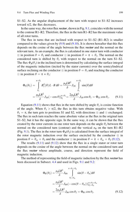
S1–S2. As the angular displacement of the turn with respect to S1–S2 increases
toward p/2, the flux decreases.
In the sameway, the rotor flux vector, shown in Fig. 9.1, coincideswith the normal
to the contour R1–R2. Therefore, the flux in the turn R1–R2 has the maximum value
of all rotor turns.
The flux in turns that are inclined with respect to S1–S2 (R1–R2) is smaller
compared to the values given by (9.9) and (9.10). It is shown hereafter that this flux
depends on the cosine of the angle between the flux vector and the normal on the
relevant turn. As an example, the flux is calculated in one stator turn with conductor
� in position y ¼ y1 and conductor � in position y ¼ p þ y1. The normal on the
considered turn is shifted by y1 with respect to the normal on the turn S1–S2.
The fluxFS(y1) in the inclined turn is determined by calculating the surface integral
of the magnetic induction (incited by the stator currents) over the semicylindrical
surface reclining on the conductor � in position y ¼ y1 and reaching the conductor� in position y ¼ p + y1:
FS y1ð Þ ¼ðpþy1
y1
BSr yð Þ L � R dy ¼ m0LR
2
dJS0
ðpþy1
y1
sin yð Þdy
¼ m0LR2
dJS0 � cos yð Þjpþy1
y1 ¼ 2m0LR2
dJS0 cos y1 ¼ FS1 cos y1: (9.11)
Equation (9.11) shows that flux in the turn shifted by angle y1 is cosine functionof the angle. When y1 > p/2, the flux in this turn obtains negative value. With
y1 ¼ p, the turn gets to positions S1 and S2, with directions � and � exchanged.
The flux in such turn reaches the same absolute value as the flux in the original turn
S1–S2, but it has the opposite sign. In the same way, it can be shown that the flux
created by the rotor currents in one rotor turn depends on the angle y2 between the
normal on the considered turn (contour) and the vertical nR on the turn R1–R2
(Fig. 9.1). The flux in the rotor turn FR(y2) is calculated from the surface integral of
the rotor magnetic induction over the surface encircled by the conductor � in
position y ¼ ym þ y2 and the conductor � in position y ¼ p þ ym þ y2 (9.12).The results (9.11) and (9.12) show that the flux in a single stator or rotor turn
depends on the cosine of the angle between the normal on the considered turn and
the flux vector whose amplitude, course, and direction represent the field of
magnetic induction.
The method of representing the field of magnetic induction by the flux vector hasbeen discussed in Subsect. 4.4 and used in Figs. 9.1 and 9.2:
FR y2ð Þ ¼ m0LR2
dJR0
ðpþy2þym
y2þym
sin y� ymð Þdy
¼ m0LR2
dJR0 � cos y� ymð Þð Þjpþy2þym
y2þym
¼ 2m0LR2
dJR0 cos y2 ¼ FR1 cos y2: (9.12)
9.4 Turn Flux and Winding Flux 199
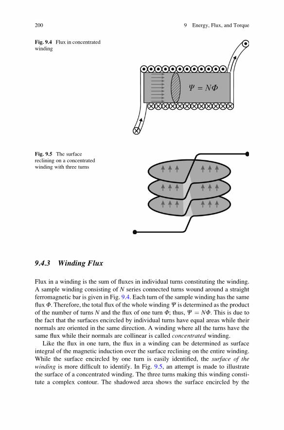
9.4.3 Winding Flux
Flux in a winding is the sum of fluxes in individual turns constituting the winding.
A sample winding consisting of N series connected turns wound around a straight
ferromagnetic bar is given in Fig. 9.4. Each turn of the sample winding has the same
fluxF. Therefore, the total flux of the whole windingC is determined as the product
of the number of turns N and the flux of one turn F; thus, C ¼ NF. This is due tothe fact that the surfaces encircled by individual turns have equal areas while their
normals are oriented in the same direction. A winding where all the turns have the
same flux while their normals are collinear is called concentrated winding.
Like the flux in one turn, the flux in a winding can be determined as surface
integral of the magnetic induction over the surface reclining on the entire winding.
While the surface encircled by one turn is easily identified, the surface of thewinding is more difficult to identify. In Fig. 9.5, an attempt is made to illustrate
the surface of a concentrated winding. The three turns making this winding consti-
tute a complex contour. The shadowed area shows the surface encircled by the
Fig. 9.4 Flux in concentrated
winding
Fig. 9.5 The surface
reclining on a concentrated
winding with three turns
200 9 Energy, Flux, and Torque
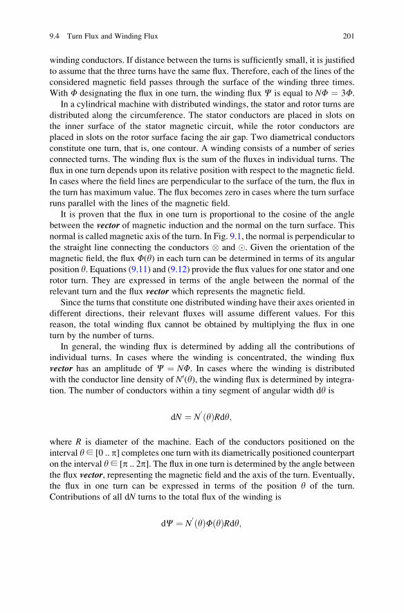
winding conductors. If distance between the turns is sufficiently small, it is justified
to assume that the three turns have the same flux. Therefore, each of the lines of the
considered magnetic field passes through the surface of the winding three times.
With F designating the flux in one turn, the winding flux C is equal to NF ¼ 3F.In a cylindrical machine with distributed windings, the stator and rotor turns are
distributed along the circumference. The stator conductors are placed in slots on
the inner surface of the stator magnetic circuit, while the rotor conductors are
placed in slots on the rotor surface facing the air gap. Two diametrical conductors
constitute one turn, that is, one contour. A winding consists of a number of series
connected turns. The winding flux is the sum of the fluxes in individual turns. The
flux in one turn depends upon its relative position with respect to the magnetic field.
In cases where the field lines are perpendicular to the surface of the turn, the flux in
the turn has maximum value. The flux becomes zero in cases where the turn surface
runs parallel with the lines of the magnetic field.
It is proven that the flux in one turn is proportional to the cosine of the angle
between the vector of magnetic induction and the normal on the turn surface. This
normal is called magnetic axis of the turn. In Fig. 9.1, the normal is perpendicular to
the straight line connecting the conductors � and �. Given the orientation of the
magnetic field, the flux F(y) in each turn can be determined in terms of its angular
position y. Equations (9.11) and (9.12) provide the flux values for one stator and onerotor turn. They are expressed in terms of the angle between the normal of the
relevant turn and the flux vector which represents the magnetic field.
Since the turns that constitute one distributed winding have their axes oriented in
different directions, their relevant fluxes will assume different values. For this
reason, the total winding flux cannot be obtained by multiplying the flux in one
turn by the number of turns.
In general, the winding flux is determined by adding all the contributions of
individual turns. In cases where the winding is concentrated, the winding flux
vector has an amplitude of C ¼ NF. In cases where the winding is distributed
with the conductor line density of N0(y), the winding flux is determined by integra-
tion. The number of conductors within a tiny segment of angular width dy is
dN ¼ N0yð ÞRdy;
where R is diameter of the machine. Each of the conductors positioned on the
interval y∈ [0 .. p] completes one turn with its diametrically positioned counterpart
on the interval y∈ [p .. 2p]. The flux in one turn is determined by the angle between
the flux vector, representing the magnetic field and the axis of the turn. Eventually,
the flux in one turn can be expressed in terms of the position y of the turn.
Contributions of all dN turns to the total flux of the winding is
dC ¼ N0yð ÞF yð ÞRdy;
9.4 Turn Flux and Winding Flux 201
while the total flux of the winding is
C ¼ðp
0
N0yð ÞF yð ÞRdy: (9.13)
Equation (9.13) can be used for calculation of the winding fluxes of both stator
and rotor windings.
An example of practical use of the (9.13) is calculation of the self-inductance of
the stator winding. Self-inductance is coefficient that defines effect of winding
currents on winding flux. In cases where the winding flux C does not have any
external originator and exists due to the winding current I only, the self-inductancecan be calculated as LS ¼ C/I. Before using (9.13), it is necessary to calculate the
flux in one turn F(y). It is calculated as the surface integral of the magnetic
induction BrS in the air gap, wherein Br
S denotes the radial component of the
magnetic inductance created by the stator currents. Dividing the flux in the stator
winding by the stator current I gives the self-inductance of the stator winding.Similar procedure can be used to determine the mutual inductance between the
stator and rotor windings. The mutual inductance Lm defines the effect of the rotor
currents on the flux in the stator winding. In cases where the rotor currents contribute
to resultant magnetic induction in the air gap, they also change the resultant flux in
the stator turns and, hence, the flux in the stator winding. The same coefficient
defines the effects of the stator currents on the flux in the rotor winding. Calculation
of Lm requires the previous procedure to be modified. When calculating the flux in
one stator turn F(y), it is necessary to replace the magnetic inductance BrS, created
by the stator currents, by the magnetic inductance BrR, created by the rotor currents.
In this way, the value ofF(y) corresponds to the flux that the rotor currents establishin one stator turn. At that time, calculation of the stator flux according to (9.13)
results in the flux created in the stator winding by action of the rotor currents.
Dividing this value by the rotor current gives coefficient of mutual inductance
between stator and rotor windings.
To proceed, the flux in the stator winding of the electrical machine shown in
Fig. 9.1 is calculated by using (9.13), assuming that the magnetic field in the air gap
is excited by the stator currents. Therefore, the magnetic field in the air gap is
calculated assuming that the rotor currents are equal to zero. Distributed winding of
the stator can be considered as a set of NT ¼ NC/2 contours, where NC denotes the
number of conductors in the stator winding while NT is the number of turns.
According to (8.2), the number of turns is equal to NT ¼ 2R N0Smax, where N0
Smax
is the maximum line density of the stator conductors, which exists at positions of
conductors S1 and S2 in Fig. 9.1.
In order to calculate the winding flux, it is necessary to calculate the flux in one
turn. For a turn with conductor � in position y and with conductor � in position
p þ y, the flux FS(y) is determined from (9.11):
FS yð Þ ¼ FS1 cos y
202 9 Energy, Flux, and Torque
Since the line density of the stator conductors is
N0yð Þ ¼ NSmax cos y;
Equation (9.13) becomes
CS ¼ðp
0
NSmax cos y � FS1 cos y � R � dy
¼ NSmaxFS1R
ðp
0
cos2y dy
¼ p2NSmaxFS1R ¼ p
4NTFS1: (9.14)
With p/4 < 1, it is concluded from (9.14) that the flux in a distributed winding
is smaller than the flux in a concentrated winding having the same number of turns.
A concentrated winding would be obtained by placing all the conductors in places
S1 and S2 (Fig. 9.1). The flux in the concentrated winding is obtained by
multiplying the number of turns NT and the flux in one turn FS1.
9.4.4 Winding Flux Vector
The winding flux can be represented by a vector denoting the course, direction, andamplitude of the flux. The winding flux vector can be obtained by adding the flux
vectors representing the fluxes in individual turns. In cases where the flux vectors ofindividual turns have different orientations, it is necessary to determine their sum
and find the course and direction for the flux vector of the winding.The convention of representing the flux in one turn by vector is presented in
Section 4.4. The course and direction of the flux vector in one turn are determined
from the normal to the surface reclining on the relevant turn. In Sect. 5.5, magnetic
axis of a winding has been defined on the basis of the course and direction of the
lines representing the magnetic field created by electrical currents in the winding
itself. The course of the winding axis is determined by positions of magnetic poles
created in the magnetic circuit due to the winding currents. The convention of
representing the magnetic field of a distributed winding by flux vector is given in
Sect. 8.5. Once again, the course and direction of the flux vector are determined
from spatial orientation of the magnetic field, that is, from positions of the magnetic
poles. Practical example of calculating the course and direction of the flux vector isgiven for the machine presented in Fig. 9.1. It starts with determining the spatial
distribution of the magnetic field created by the currents in distributed winding.
Direction of the winding flux vector is determined on the basis of direction of the
9.4 Turn Flux and Winding Flux 203
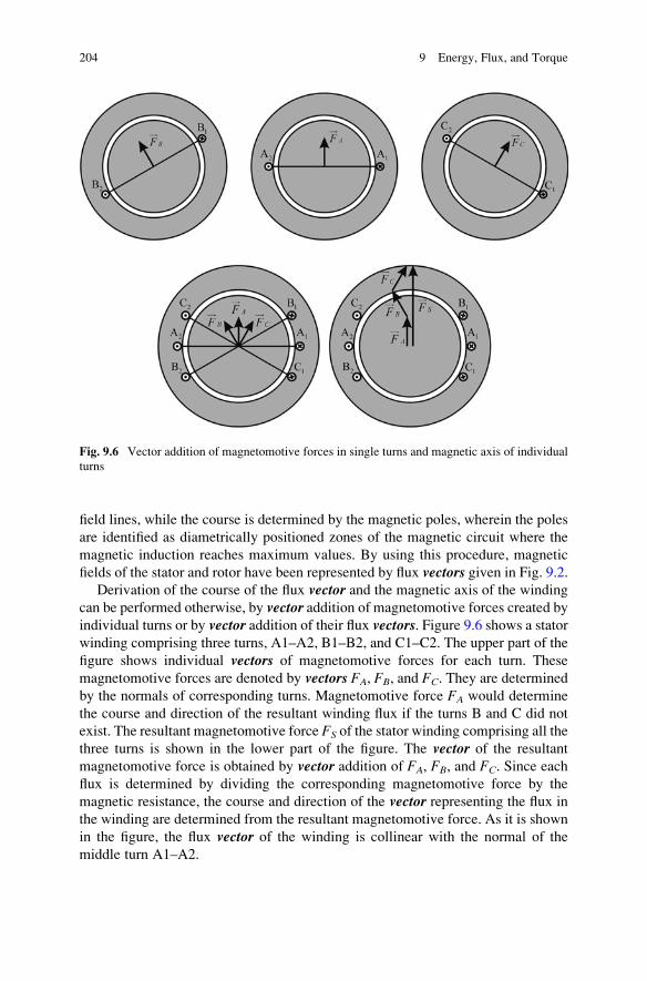
field lines, while the course is determined by the magnetic poles, wherein the poles
are identified as diametrically positioned zones of the magnetic circuit where the
magnetic induction reaches maximum values. By using this procedure, magnetic
fields of the stator and rotor have been represented by flux vectors given in Fig. 9.2.Derivation of the course of the flux vector and the magnetic axis of the winding
can be performed otherwise, by vector addition of magnetomotive forces created by
individual turns or by vector addition of their flux vectors. Figure 9.6 shows a statorwinding comprising three turns, A1–A2, B1–B2, and C1–C2. The upper part of the
figure shows individual vectors of magnetomotive forces for each turn. These
magnetomotive forces are denoted by vectors FA, FB, and FC. They are determined
by the normals of corresponding turns. Magnetomotive force FA would determine
the course and direction of the resultant winding flux if the turns B and C did not
exist. The resultant magnetomotive force FS of the stator winding comprising all the
three turns is shown in the lower part of the figure. The vector of the resultant
magnetomotive force is obtained by vector addition of FA, FB, and FC. Since each
flux is determined by dividing the corresponding magnetomotive force by the
magnetic resistance, the course and direction of the vector representing the flux in
the winding are determined from the resultant magnetomotive force. As it is shown
in the figure, the flux vector of the winding is collinear with the normal of the
middle turn A1–A2.
Fig. 9.6 Vector addition of magnetomotive forces in single turns and magnetic axis of individual
turns
204 9 Energy, Flux, and Torque
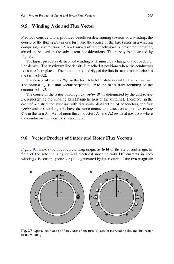
9.5 Winding Axis and Flux Vector
Previous considerations provided details on determining the axis of a winding, the
course of the flux vector in one turn, and the course of the flux vector in a winding
comprising several turns. A brief survey of the conclusions is presented hereafter,
aimed to be used in the subsequent considerations. The survey is illustrated by
Fig. 9.7.
The figure presents a distributed winding with sinusoidal change of the conductor
line density. The maximum line density is reached at positions where the conductors
A1 and A2 are placed. The maximum value FS1 of the flux in one turn is reached in
the turn A1–A2.
The course of the flux FS1 in the turn A1–A2 is determined by the normal nS1.The normal nS1 is a unit vector perpendicular to the flat surface reclining on the
contour A1–A2.
The course of the stator winding flux vectorCS is determined by the unit vectornS, representing the winding axis (magnetic axis of the winding). Therefore, in the
case of a distributed winding with sinusoidal distribution of conductors, the flux
vector and the winding axis have the same course and direction as the flux vectorFS1 in the turn A1–A2, wherein the conductors A1 and A2 reside at positions where
the conductor line density is maximum.
9.6 Vector Product of Stator and Rotor Flux Vectors
Figure 9.1 shows the lines representing magnetic field of the stator and magnetic
field of the rotor in a cylindrical electrical machine with DC currents in both
windings. Electromagnetic torque is generated by interaction of the two magnetic
Fig. 9.7 Spatial orientation of flux vector of one turn (a), axis of the winding (b), and flux vector
of the winding
9.6 Vector Product of Stator and Rotor Flux Vectors 205
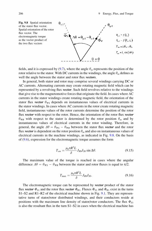
fields, and it is expressed by (9.7), where the angle ym represents the position of the
rotor relative to the stator. With DC currents in the windings, the angle ym defines as
well the angle between the stator and rotor flux vectors.In general, both stator and rotor may comprise several windings carrying DC or
AC currents. Alternating currents may create rotating magnetic field which can be
represented by a revolving flux vector. Such field revolves relative to the windings
that give rise to the magnetomotive forces that originate the field. In cases where AC
currents in the stator windings create rotating magnetic field, the orientation of the
stator flux vector yCS depends on instantaneous values of electrical currents in
the stator windings. In cases where AC currents in the rotor create rotating magnetic
field, instantaneous values of the rotor currents determine the position of the rotor
flux vector with respect to the rotor. Hence, the orientation of the rotor flux vectoryCR with respect to the stator is determined by the rotor position ym and by
instantaneous values of electrical currents in the rotor winding. Therefore, in
general, the angle Dy ¼ yCS � yCR between the stator flux vector and the rotor
flux vector is dependent on the rotor position ym and also on instantaneous values of
electrical currents in the machine windings, as indicated in Fig. 9.8. On the basis
of (9.6), expression for the electromagnetic torque assumes the form
Tem ¼ m0pR3L
dJR0JS0 sinDy: (9.15)
The maximum value of the torque is reached in cases where the angular
difference Dy ¼ yCS � yCR between the stator and rotor fluxes is equal to p/2.
Tmax ¼ m0pR3L
dJR0JS0: (9.16)
The electromagnetic torque can be represented by vector product of the stator
flux vector FS1 and the rotor flux vector FR1. Fluxes FS1 and FR1 exist in the turns
S1–S2 and R1–R2 of the electrical machine shown in Fig. 9.1. They are represen-
tative turns of stator/rotor distributed windings, and their conductors reside at
positions with the maximum line density of stator/rotor conductors. The flux FS1
is also the resultant flux in the turn S1–S2 in cases when the electrical machine has
Fig. 9.8 Spatial orientation
of the stator flux vector.
Spatial orientation of the rotor
flux vector. The
electromagnetic torque
as the vector product of
the two flux vectors
206 9 Energy, Flux, and Torque
only the stator currents, while the flux FR1 is also the resultant in the turn R1–R2 in
cases where only the rotor currents exist in the machine. On the basis of (9.9) and
(9.10), amplitudes of the two vectors are determined by expressions
FS1 ¼ 2m0LR2
dJS0; FR1 ¼ 2m0LR
2
dJR0:
Since the torque is expressed by function sin Dy, it can be calculated as the
vector product of the stator and rotor flux vectors. Expression for the torque can be
represented in the form
m0pR3L
dJR0JS0 sinDy ¼ pd
4m0LR
� �2m0LR
2
dJS0
� �2m0LR
2
dJR0
� �sinDy
which comprises the amplitude of the vector product of the stator and rotor flux
vectors, given by (9.17),
~Tem ¼ pd4m0LR
� �� ~FR � ~FS
h i¼ k ~FR � ~FS
h i(9.17)
where the constant k is
k ¼ pd4m0LR
:
Since the flux vectors FS1 and FR1 of the turns S1–S2 and R1–R2 have the same
spatial orientation as the flux vectors of the stator and rotor windings, respectively,
the electromagnetic torque can be expressed as the vector product CS � CR of the
flux vectorCS in the stator winding and the flux vectorCR in the rotor winding. On
the basis of (9.14), the amplitudes of vectors CS and CR are determined by
expressions
CS ¼ p4NTSFS1; CR ¼ p
4NTRFR1;
where NTS and NTR denote the number of turns of the stator and rotor windings,
respectively. Since the flux vectors of the representative turns are collinear with theflux vectors of respective windings, (9.17) takes the form
~Tem ¼ pd4m0LR
� �� ~FR � ~FS
h i
¼ pd4m0LR
� �� 4
pNTS
� �4
pNTR
� �~CR � ~CS
h i
¼ 4dm0pLRNTSNTR
� �� ~CR � ~CS
h i
¼ k1 � ~CR � ~CS
h i; (9.18)
9.6 Vector Product of Stator and Rotor Flux Vectors 207
where k1 is constant equal to
k1 ¼ 4dm0pLRNTSNTR
:
Equations (9.17) and (9.18) give the vector of electromagnetic torque. The
course of the obtained vector is determined by axis z of the cylindrical coordinatesystem, that is, by the axis of rotor revolutions. Direction of the torque vector is inaccordance with the reference direction of z-axis. The torque of a positive value actstoward increasing the rotor speed Om and moves the rotor toward increasing the
angle ym, which corresponds to the movement in counterclockwise direction.
The torque amplitude is determined by equation
Tem ¼ k ~FR � ~FS
�� ��:
Question (9.3): Expression for the torque (9.7) has the leading minus sign. Should
the torque of a negative value be expected in the case represented in Fig. 9.1? Why
(9.15) does not include negative sign?
Answer (9.3): The electromagnetic torque is determined by the function sin Dy,where Dy is the angle equal to yCS � yCR. The angles yCS and yCR determine the
course of the stator and rotor flux vectors. In Fig. 9.1, courses of the two flux vectorsare shown assuming that the windings carry a constant DC current. Then yCS ¼ p/2,while yCR ¼ p/2 þ ym, resulting inDy ¼ �ym. In the considered case, the torque isproportional to function sin Dy ¼ �sin ym, which gives the minus sign in (9.7).
9.7 Conditions for Torque Generation
The electromagnetic torque can be calculated from the vector product of the flux
vector FS1 and the flux vector FR1, wherein the former is created by the stator
currents in the stator turn S1–S2 while the latter is created by the rotor currents in
the turn R1–R2 (Fig. 9.1). The expression for the electromagnetic torque is given by
(9.17). Equation (9.18) reformulates the expression by introducing the vectorproduct of the stator flux vector and the rotor flux vector.
The torque is proportional to the sine of the angle Dy between the relevant flux
vectors. With DC currents in both the stator and the rotor windings, the stator
flux does not move with respect to the stator while the rotor flux does not move with
respect to the rotor. In this case, the stator flux is leading with respect to the rotor
flux by Dy ¼ �ym.With the rotor revolving at a constant angular speed Om, and with the initial rotor
position ym(0) ¼ 0, the rotor position changes as ym(t) ¼ Omt. Therefore, the anglebetween the stator flux vector and the rotor flux vector is Dy ¼ �ym ¼ �Omt.
208 9 Energy, Flux, and Torque
Hence, electrical machine with both stator and rotor windings carrying DC current
develops electromagnetic torque proportional to sin(Omt). The average value of thistorque and the average value of the corresponding conversion power Pem ¼ Tem Om
are both equal to zero. Therefore, an electrical machine with DC currents in the
stator and in the rotor windings cannot provide an average power other than zero.
A nonzero average value of the torque is obtained in cases where the angle Dybetween the stator and rotor flux vectors is constant. For the given winding currents,the electromagnetic torque has the maximum value with Dy ¼ p/2.
Condition Dy ¼ const. cannot be achieved with both the stator and rotor
windings carrying DC currents. It will be proven later on that at least one of the
windings on either stator or rotor must have AC currents and create the revolving
magnetic field. There are three distinct cases when the constraint Dy ¼ const. is
fulfilled. These three methods of accomplishing constant relative position of the
two flux vectors have been shown in Fig. 7.8. These examples are reinstated
hereafter and explained again in terms of the flux vectors.It is of interest to notice that a nonzero average value of the electromagnetic
torque is achieved only in cases where the angle Dy ¼ yCS � yCR is constant.
Namely, the stator and rotor flux vectorsmust retain their relative position. Whether
they revolve or stay firm, the angle between flux vectors representing the stator androtor magnetic fields must not change. There are three cases where this condition is
fulfilled:
(a) Stator field is still with respect to stator. Rotor field rotates with respect to rotor
in the opposite direction of rotation of rotor; thus, rotor field does not move with
respect to stator.
(b) Stator field rotates with respect to stator. Rotor field rotates with respect to
rotor. Sum of rotor speed relative to stator and rotor field speed relative to rotor
is equal to speed of rotation of stator field relative to stator.
(c) Stator field rotates with respect to stator at speed equal to rotor speed. Rotor
field does not move with respect to rotor.
Generation of stator or rotor magnetic field which does not rotate with respect to
originating windings can be done by one or more windings with DC currents.
Generation of the field that revolves with respect to originating windings requires
at least two windings of different spatial orientation and with AC currents of the
appropriate frequency and initial phase. Conditions for creation of a rotating field
have been discussed in the section devoted to rotating field.
Case (a) corresponds to direct current machines (DCmachines), and it is shown in
Fig. 7.8a. Vector of the stator flux does not move with respect to the stator because
the stator conductors have constant DC currents. The torque generation requires the
rotor flux to retain its relative position to the stator flux. This means that the rotor flux
vector in Fig. 7.8a should not move either. For the rotor flux vector to remain still
while the rotor windings revolve, electrical currents in rotor conductors should
create magnetic field which rotates with respect to the rotor at the speed �Om.
In this case, the rotor revolves in positive direction at the speedþOm, while the rotor
flux revolves with respect to the rotor in the opposite direction. Therefore, the
9.7 Conditions for Torque Generation 209
rotor flux remains still with respect to the stator. For the rotor windings to create
revolving field, the rotor must have AC currents, the frequency of which is deter-
mined by the speed of rotation. Yet, DC machines are supplied from DC power
sources. In order to convert DC supply currents into AC rotor currents, DCmachines
have a mechanical commutator, device with brushes attached to the stator and
collector attached to the rotor. Collector has a number of isolated segments,
connected to the rotor conductors. When the rotor revolves, the segments slide
under the brushes, altering electrical connections and changing the way of injecting
the supply current into the rotor winding. In such way, commutator directs DC
current of the electrical power source into rotor conductors in such way that the rotor
conductors have AC currents. The frequency of these currents is determined by the
speed of rotation. The commutator will be explained in more detail in the chapter on
DC machines. Thanks to the commutator, the flux vector FR1 remains still with
respect to flux vector FS1; thus, the angle Dy remains constant.
Case (b) shown in Fig. 7.8b corresponds to asynchronous machines. Windings of
the stator and rotor have AC currents of angular frequency os and ok, respectively.
The stator flux vector rotates with respect to the stator at the speed Os, determined by
the angular frequency os. The rotor flux vector rotates with respect to the rotor at thespeed ofOk, determined by the angular frequency ok. Difference os � ok in angular
frequency determines the rotor speedOm. The flux vectors of the stator and rotor rotateat the same speed (Os). Consequently, their mutual position Dy does not change.
Case (c) shown in Fig. 7.8c corresponds to synchronousmachines. There are rotor
windings with constant DC currents producing the rotor flux. Alternatively, the rotor
does not have any windings. Instead, there are permanent magnets mounted on the
rotor. In either case, the rotor flux vector FR1 rotates at the same speed as the rotor
does. The stator of the machine has a system of windings with two or more phases
carrying AC currents. Angular frequency os of the stator currents creates the stator
magnetic field which revolves at the speed Os, determined by the angular frequency
os of the stator currents. In synchronous machines, the stator frequency ensures that
the field rotates at the same speed as the rotor, that is, Os ¼ Om. Therefore, the flux
vectors FR1 and FS1 rotate at the same speed, and their mutual position Dy does
not change.
Question (9.4): Derive the expression for the torque acting on a contour with
electrical current in a homogenous magnetic field, with the normal to the contour
being inclined with an angle y with respect to the vector B, as shown in Fig. 3.6. Thecontour is circular, with diameter D and with electrical current I. Assume that
the contour revolves around the axis which is orthogonal to the direction of the
field. The speed of rotation is known and constant. Determine the instantaneous and
average value of the torque acting on the contour. Assuming that the magnetic
field cannot be changed, but it is possible to have an arbitrary current in the contour,
determine the current i(t) whichwould result in a nonzero average value of the torque.With the assumption that the induction B(t) is variable while the electrical
current i(t) ¼ I is constant, determine one solution for B(y) which results in a
nonzero average value of the torque.
210 9 Energy, Flux, and Torque
Answer (9.4): The electromagnetic torque Tem acting on the contour is equal to
I�B�S�siny. When the contour rotates at angular speed O while both the current and
magnetic inductance are constant, the torque varies according to function sin(O t),and its average value is zero. In cases where the magnetic induction is constant
while the current i(t) ¼ I sin(ot) changes with angular frequency o equal to the
speed of rotation O, the torque is proportional to (sin(ot))2 and has a nonzero
average value. If the contour has a constant current I, nonzero average of the torquecan be obtained in cases when the magnetic induction changes as B(t) ¼ Bm�sin(ot), where the angular frequency o corresponds to the speed of rotation O.
9.8 Torque–Size Relation
Expression for electromagnetic torque (9.16) shows that the torque is proportional
to R3L, that is, to the axial length of the machine L and third power of its diameterD.Diameter and axial length are linear dimensions of the machine, and common
notation l can be used for both. Therefore, the electromagnetic torque is propor-
tional to fourth power of the linear dimensions l of the machine, T ~ l4. Volume of
the machine is proportional to the third power of linear dimensions, V ~ l3. There-fore, the torque is proportional to T ~ V4/3.
Electrical machines are made of iron and copper, materials of known specific
masses.1 Therefore, the mass m of an electrical machine is determined by the
electromagnetic torque for which it has been designed. The mass m and torque Tare related by T ~ m4/3. As an example, a new machine with all the three
dimensions doubled with respect to the original machine develops electromagnetic
torque increase 24 ¼ 16 times.
Relation T ~ m4/3 can be verified in another way. It has been proven that the
torque can be expressed as vector product of two flux vectors. The flux amplitude
depends on the surface (S ~ l2) and magnetic induction (B < Bmax), the latter being
limited by magnetic saturation of the ferromagnetic material and not exceeding
1.5 . 1.7 Т. The product of two fluxes depends on the fourth power of linear dimension
l. Hence, the product of stator and rotor flux vectors depends on l4. Hence, theelectromagnetic torque available from electrical machine is proportional to l4.
Power of electromechanical conversion in an electrical machine depends on the
torque and speed of rotation O; therefore, P ~ V4/3O. Considering two machines
with the same dimensions and different speeds, the one with the higher speed
delivers more power. In cases requiring a constant power of electromechanical
conversion P, while the speed of rotation of the electrical machine can be arbitrarily
chosen, it is beneficial to select the machine with higher speed, resulting in a lower
torque T ¼ P/O and consequently smaller dimensions of the machine due to T ~ l4.An example where the required load speed can be achieved with different machine
1 gFe ¼ DmFe/DV ¼ 7,874 kg/m3, gCu ¼ DmCu/DV ¼ 8,020 kg/m3.
9.8 Torque–Size Relation 211
speeds is the case where the load and the machine are coupled by gears. While
designing the system, the gear ratio can be selected so as to result in a higher speed
of the machine. This will reduce the size and weight of the machine.
The torque expression (9.16) suggests that the torque is inversely proportional to
the air gap width d. With constant stator and rotor currents, a decrease in the air gap
results in an increase in electromagnetic torque. The expression suggests that the
torque can be increased with no apparent limits, provided that the air gap d can get
sufficiently small. This conclusion is incorrect as it overlooks the phenomenon of
magnetic saturation. The expression for the torque has been derived as a result of an
analysis wheremagnetic saturation in iron is neglected. The stator and rotor magnetic
circuits are made of iron sheets of very high permeability mFe, making the magnetic
field in iron HFe negligible. The torque expression (9.16) is based on such an
assumption. It holds in all the conditions with no magnetic saturation in iron parts
of themagnetic circuit.With excessive values ofBFe resulting inmagnetic saturation,
the value of HFe cannot be neglected, and this invalidates the (9.16). The preceding
analysis finds themagnetic inductionB0 in the air gap inversely proportional to the air
gap d. Disregarding the slots, the magnetic induction in iron is roughly the same,
BFe B0. Therefore, progressive decrease of the air gap leads to increased magnetic
induction. As the magnetic induction B reaches Bmax ¼ 1.5 .. 1.7 T, the iron gets
saturated, permeability mFe drops, and the magnetic field HFe assumes considerable
value that cannot be neglected. At this point, (9.15) and the consequential results,
obtained by neglecting saturation, are not valid and cannot be used.
The air gap of electrical machines is designed to be as small as possible, in order
to obtained the desired magnetic induction B0 with smaller electrical currents and,
consequently, smaller copper losses. However, there are limitations of mechanical
nature which prevent the air gap of smaller machines from getting much below one
millimeter. The air gap of large electrical machines is at least several millimeters.
A lower limit of the air gap is required to prevent the revolving rotor from touching
the stator. Undesired touching and scratching can happen due to finite tolerances
in manufacturing the stator and rotor surfaces. Elastic deformation of the shaft in
radial direction can result in rotor touching the stator. These phenomena prevent the
use of electrical machines with very small air gaps.
Question (9.5): The expressions for the electromagnetic torque and power of
electrical machine give values inversely proportional to the air gap d. Based on
these expressions, the power and torque can be increased with no apparent limits,
keeping the electrical currents constant and reducing the air gap. There are reasons
that invalidate such conclusion. Provide two reasons which indicate that such
expectations are not realistic.
Answer (9.5): The expression for the electromagnetic torque suggests that reduc-
tion of the air gap d results in higher torque and higher power of electromechanical
conversion. Apparently, very high torque can be achieved with an adequate reduc-
tion of the air gap.
This conclusion overlooks the phenomenon of magnetic saturation. The torque
expression comes from an analysis that starts with an assumption that the magnetic
212 9 Energy, Flux, and Torque
field HFe in iron is negligible. This assumption holds only in cases where the flux
density BFe does not reach the saturation limit of Bmax ¼ 1.5 .. 1.7 T. Namely, given
a magnetomotive force Ni ¼ 2Hd, the flux density B ¼ m0Ni/(2d) grows as the airgap decreases. As the flux density B reaches the saturation limit Bmax, any further
increase of BFe is determined by expression DB ¼ m0DH. In other words, differen-
tial permeability DB/DH of the saturated ferromagnetic material is close to m0.Considering the flux changes, magnetic saturation is equivalent to removing the
iron parts of the stator and rotor magnetic circuits. Due to DB/DH m0, saturatediron behaves like air. Therefore, the magnetic saturation can be considered as a very
large increase in the air gap. Therefore, the initial projections of the air gap
reduction leading to large torque gains are not realistic. It is of interest to notice
that most electrical machines are designed so as to get the most out of their
magnetic circuits. For this to achieve, the flux density levels are close to saturation
limits. Therefore, there is no margin to accommodate any further increase in B.Another reason that prevents the torque increase is the fact that the air gap cannot
be decreased below certain limits, roughly 1 mm, imposed bymechanical conditions.
9.9 Rotating Magnetic Field
According to previous considerations, conditions for generating a nonzero average
electromagnetic torque include a constant relative position Dy of the stator and
rotor flux vectors. In DC machines, both flux vectors remain still with respect to the
stator. In alternating current machines, whether asynchronous or synchronous, both
flux vectors rotate at the same speed.
In order to meet the above condition and due to rotor revolution, at least one of
the two fluxes (FS orFR) has to rotate with respect to the winding that originates the
magnetomotive force resulting in the relevant flux. The magnetic field which
rotates with respect to the originating windings is also called rotating magneticfield. In this section, it is shown that rotating magnetic field requires a system
with at least two separate windings with appropriate spatial displacement of their
magnetic axes. Alternating currents in the windings should have the same fre-
quency and amplitude. Their initial phases are to be different and should correspond
to the spatial displacement of the magnetic axes. In this case, the system of
windings creates magnetomotive force and flux that revolve at the speed deter-
mined by the frequency of AC currents.
9.9.1 System of Two Orthogonal Windings
Electromagnetic torque is determined by the vector product of the stator and rotor
flux vectors, and it depends on sine of the angle Dy between the two vectors.A continuous conversion of energy with constant torque and constant power
9.9 Rotating Magnetic Field 213
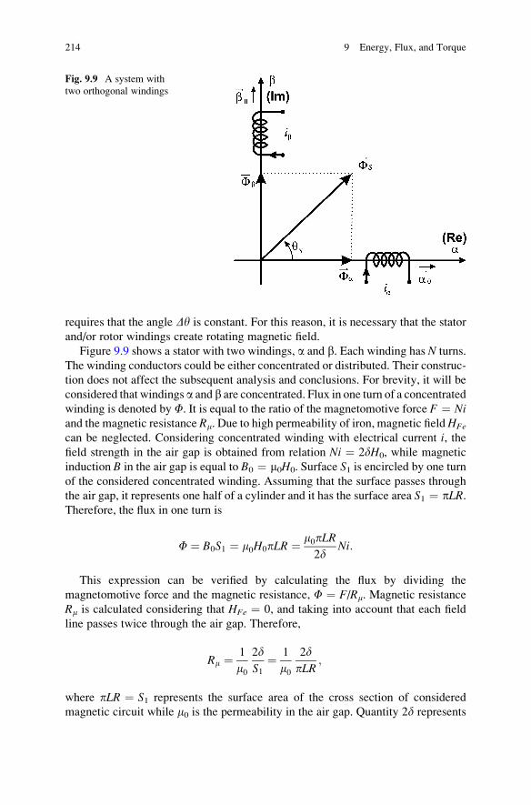
requires that the angle Dy is constant. For this reason, it is necessary that the stator
and/or rotor windings create rotating magnetic field.
Figure 9.9 shows a stator with two windings, a and b. Each winding has N turns.
The winding conductors could be either concentrated or distributed. Their construc-
tion does not affect the subsequent analysis and conclusions. For brevity, it will be
considered that windings a and b are concentrated. Flux in one turn of a concentratedwinding is denoted by F. It is equal to the ratio of the magnetomotive force F ¼ Niand the magnetic resistance Rm. Due to high permeability of iron, magnetic fieldHFe
can be neglected. Considering concentrated winding with electrical current i, thefield strength in the air gap is obtained from relation Ni ¼ 2dH0, while magnetic
induction B in the air gap is equal to B0 ¼ m0H0. Surface S1 is encircled by one turnof the considered concentrated winding. Assuming that the surface passes through
the air gap, it represents one half of a cylinder and it has the surface area S1 ¼ pLR.Therefore, the flux in one turn is
F ¼ B0S1 ¼ m0H0pLR ¼ m0pLR2d
Ni:
This expression can be verified by calculating the flux by dividing the
magnetomotive force and the magnetic resistance, F ¼ F/Rm. Magnetic resistance
Rm is calculated considering that HFe ¼ 0, and taking into account that each field
line passes twice through the air gap. Therefore,
Rm ¼ 1
m0
2dS1
¼ 1
m0
2dpLR
;
where pLR ¼ S1 represents the surface area of the cross section of considered
magnetic circuit while m0 is the permeability in the air gap. Quantity 2d represents
Fig. 9.9 A system with
two orthogonal windings
214 9 Energy, Flux, and Torque
the length of the magnetic circuit where the field strength H assumes considerable
values and the line integral of the field results in magnetic voltage drop. The air gapis passed twice, where the field lines enter and exit the rotor (or stator) magnetic
circuit, that is, next to the north and south magnetic poles. Expression F ¼ F/Rm
becomes
F ¼ F
Rm¼ Ni
1m0
2dpLR
¼ m0pLR2d
Ni: (9.19)
Magnetic axes of the windings a and b reside on the abscissa and ordinate of the
orthogonal coordinate system shown in Fig. 9.9. Axis of the winding a is horizontal,
along the course defined by the unit vector a0. By establishing electrical current ia,magnetomotive force Fa ¼ Nia is produced along the course and direction of the
unit vector a0. The flux in one turn is obtained by dividing the magnetomotive
force and the magnetic resistance, Fa ¼ Nia/Rm. It is assumed that the windings
are concentrated; thus, the flux Ca in the winding is equal to NFa ¼ N2ia/Rm. The
axis of the winding b is orthogonal with respect to the a winding, and it extends
along the course defined by the unit vector b0. The magnetomotive force Fb and the
flux Fb of this winding are oriented in accordance with the ordinate axis b, and it isproportional to the winding current ib. By using the unit vectors of the two axes,
fluxes in the winding turns can be represented by expressions
~Fa ¼ N
Rmia �~a0; ~Fb ¼ N
Rmib �~b0:
Electrical currents in windings a and b are alternating currents of the same
amplitude Im and the same angular frequency os. The symbol os denotes the
angular frequency of electrical currents in the stator windings. The initial phases
of the two currents are different. The current in winding a leads by p/2, the anglethat corresponds to the spatial shift between a and b magnetic axes. Variation of
currents in the windings is given by (9.20):
ia ¼ Im cos oStð Þ ¼ Im cos yS;
ib ¼ Im cos oSt� p2
¼ Im sin oStð Þ ¼ Im sin yS: (9.20)
The resultant magnetomotive force FS of the stator winding and the stator flux
FS are obtained by summing their a and b components. If the orthogonal windings
a and b in Fig. 9.9 have electrical currents as given by (9.20), the magnetomotive
force vector FS is created, determined by expression (9.21), resulting in the flux
vector given in (9.22). Since a and b components are proportional to functions cosysand sinys, where the angle ys changes as ost, the latter equation describes the flux
vector which rotates at the speed of os and has an amplitude which is constant.
Equation (29.22) gives the resultant flux corresponding to one turn. Since a
9.9 Rotating Magnetic Field 215
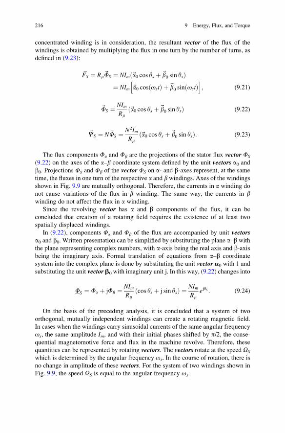
concentrated winding is in consideration, the resultant vector of the flux of the
windings is obtained by multiplying the flux in one turn by the number of turns, as
defined in (9.23):
~FS ¼ Rm~FS ¼ NImð~a0 cos ys þ~b0 sin ysÞ¼ NIm ~a0 cos ostð Þ þ~b0 sin ostð Þ
h i; (9.21)
~FS ¼ NImRm
ð~a0 cos ys þ~b0 sin ysÞ (9.22)
~CS ¼ N~FS ¼ N2ImRm
ð~a0 cos ys þ~b0 sin ysÞ: (9.23)
The flux components Fa and Fb are the projections of the stator flux vector FS
(9.22) on the axes of the a–b coordinate system defined by the unit vectors a0 andb0. Projections Fa and Fb of the vector FS on a- and b-axes represent, at the same
time, the fluxes in one turn of the respective a and bwindings. Axes of the windings
shown in Fig. 9.9 are mutually orthogonal. Therefore, the currents in a winding do
not cause variations of the flux in b winding. The same way, the currents in bwinding do not affect the flux in a winding.
Since the revolving vector has a and b components of the flux, it can be
concluded that creation of a rotating field requires the existence of at least two
spatially displaced windings.
In (9.22), components Fa and Fb of the flux are accompanied by unit vectorsa0 and b0. Written presentation can be simplified by substituting the plane a–b with
the plane representing complex numbers, with a-axis being the real axis and b-axisbeing the imaginary axis. Formal translation of equations from a–b coordinate
system into the complex plane is done by substituting the unit vector a0 with 1 and
substituting the unit vector b0 with imaginary unit j. In this way, (9.22) changes into
FS ¼ Fa þ jFb ¼ NImRm
ðcos ys þ j sin ysÞ ¼ NImRm
ejyS : (9.24)
On the basis of the preceding analysis, it is concluded that a system of two
orthogonal, mutually independent windings can create a rotating magnetic field.
In cases when the windings carry sinusoidal currents of the same angular frequency
os, the same amplitude Im, and with their initial phases shifted by p/2, the conse-
quential magnetomotive force and flux in the machine revolve. Therefore, these
quantities can be represented by rotating vectors. The vectors rotate at the speed OS
which is determined by the angular frequency os. In the course of rotation, there is
no change in amplitude of these vectors. For the system of two windings shown in
Fig. 9.9, the speed OS is equal to the angular frequency os.
216 9 Energy, Flux, and Torque
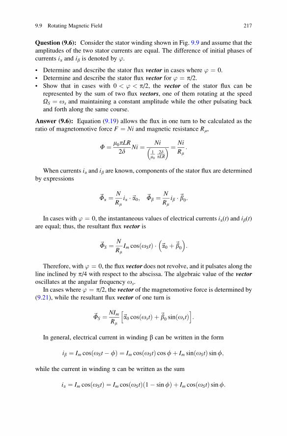
Question (9.6): Consider the stator winding shown in Fig. 9.9 and assume that the
amplitudes of the two stator currents are equal. The difference of initial phases of
currents ia and ib is denoted by ’.
• Determine and describe the stator flux vector in cases where ’ ¼ 0.
• Determine and describe the stator flux vector for ’ ¼ p/2.• Show that in cases with 0 < ’ < p/2, the vector of the stator flux can be
represented by the sum of two flux vectors, one of them rotating at the speed
OS ¼ os and maintaining a constant amplitude while the other pulsating back
and forth along the same course.
Answer (9.6): Equation (9.19) allows the flux in one turn to be calculated as the
ratio of magnetomotive force F ¼ Ni and magnetic resistance Rm,
F ¼ m0pLR2d
Ni ¼ Ni
1m0
2dpLR
¼ Ni
Rm:
When currents ia and ib are known, components of the stator flux are determined
by expressions
~Fa ¼ N
Rmia �~a0; ~Fb ¼ N
Rmib �~b0:
In cases with ’ ¼ 0, the instantaneous values of electrical currents ia(t) and ib(t)are equal; thus, the resultant flux vector is
~FS ¼ N
RmIm cos oStð Þ � ~a0 þ~b0
:
Therefore, with ’ ¼ 0, the flux vector does not revolve, and it pulsates along theline inclined by p/4 with respect to the abscissa. The algebraic value of the vectoroscillates at the angular frequency os.
In cases where ’ ¼ p/2, the vector of the magnetomotive force is determined by
(9.21), while the resultant flux vector of one turn is
~FS ¼ NImRm
~a0 cos ostð Þ þ~b0 sin ostð Þh i
:
In general, electrical current in winding b can be written in the form
ib ¼ Im cos oSt� fð Þ ¼ Im cos oStð Þ cosfþ Im sin oStð Þ sinf;
while the current in winding a can be written as the sum
ia ¼ Im cos oStð Þ ¼ Im cos oStð Þ 1� sinfð Þ þ Im cos oStð Þ sinf:
9.9 Rotating Magnetic Field 217
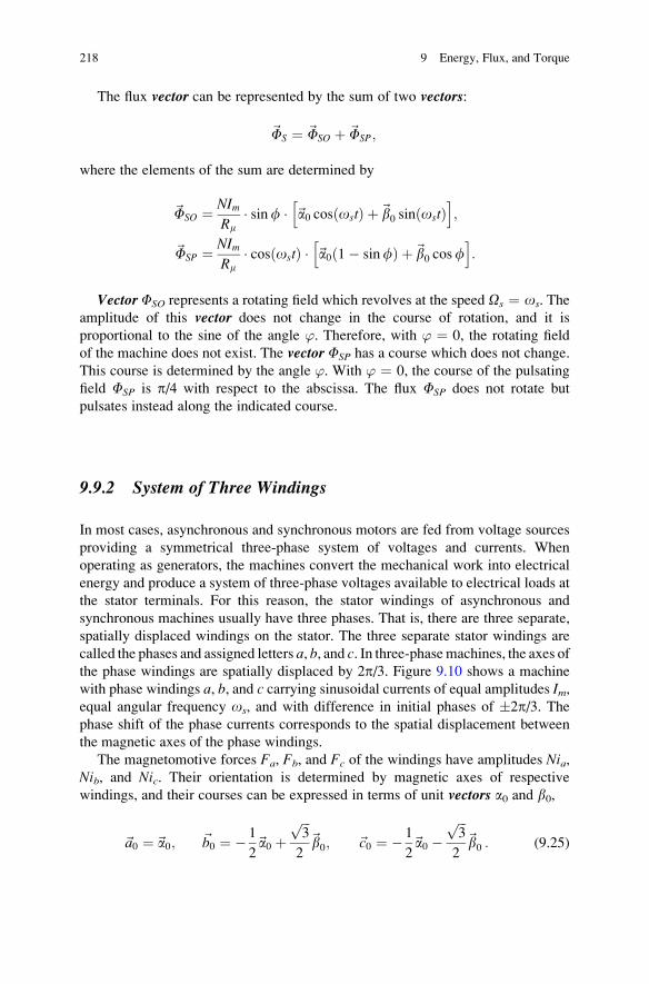
The flux vector can be represented by the sum of two vectors:
~FS ¼ ~FSO þ ~FSP;
where the elements of the sum are determined by
~FSO ¼ NImRm
� sinf � ~a0 cos ostð Þ þ~b0 sin ostð Þh i
;
~FSP ¼ NImRm
� cos ostð Þ � ~a0 1� sinfð Þ þ~b0 cosfh i
:
Vector FSO represents a rotating field which revolves at the speed Os ¼ os. The
amplitude of this vector does not change in the course of rotation, and it is
proportional to the sine of the angle ’. Therefore, with ’ ¼ 0, the rotating field
of the machine does not exist. The vector FSP has a course which does not change.
This course is determined by the angle ’. With ’ ¼ 0, the course of the pulsating
field FSP is p/4 with respect to the abscissa. The flux FSP does not rotate but
pulsates instead along the indicated course.
9.9.2 System of Three Windings
In most cases, asynchronous and synchronous motors are fed from voltage sources
providing a symmetrical three-phase system of voltages and currents. When
operating as generators, the machines convert the mechanical work into electrical
energy and produce a system of three-phase voltages available to electrical loads at
the stator terminals. For this reason, the stator windings of asynchronous and
synchronous machines usually have three phases. That is, there are three separate,
spatially displaced windings on the stator. The three separate stator windings are
called the phases and assigned letters a, b, and c. In three-phasemachines, the axes of
the phase windings are spatially displaced by 2p/3. Figure 9.10 shows a machine
with phase windings a, b, and c carrying sinusoidal currents of equal amplitudes Im,equal angular frequency os, and with difference in initial phases of 2p/3. Thephase shift of the phase currents corresponds to the spatial displacement between
the magnetic axes of the phase windings.
The magnetomotive forces Fa, Fb, and Fc of the windings have amplitudes Nia,Nib, and Nic. Their orientation is determined by magnetic axes of respective
windings, and their courses can be expressed in terms of unit vectors a0 and b0,
~a0 ¼~a0; ~b0 ¼ � 1
2~a0 þ
ffiffiffi3
p
2~b0; ~c0 ¼ � 1
2~a0 �
ffiffiffi3
p
2~b0 : (9.25)
218 9 Energy, Flux, and Torque
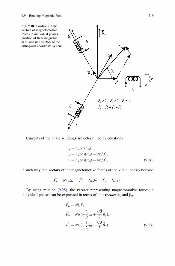
Currents of the phase windings are determined by equations
ia ¼ Im cosoSt;
ib ¼ Im cosðoSt� 2p=3Þ;ic ¼ Im cosðoSt� 4p=3Þ; (9.26)
in such way that vectors of the magnetomotive forces of individual phases become
~Fa ¼ Nia~a0; ~Fb ¼ Nib~b0; ~Fc ¼ Nic~c0:
By using relation (9.25), the vectors representing magnetomotive forces in
individual phases can be expressed in terms of unit vectors a0 and b0,
~Fa ¼ Nia~a0;
~Fb ¼ Nibð� 1
2~a0 þ
ffiffiffi3
p
2~b0Þ;
~Fc ¼ Nicð� 1
2~a0 �
ffiffiffi3
p
2~b0Þ: (9.27)
Fig. 9.10 Positions of the
vectors of magnetomotive
forces in individual phases,
position of their magnetic
axes, and unit vectors of the
orthogonal coordinate system
9.9 Rotating Magnetic Field 219
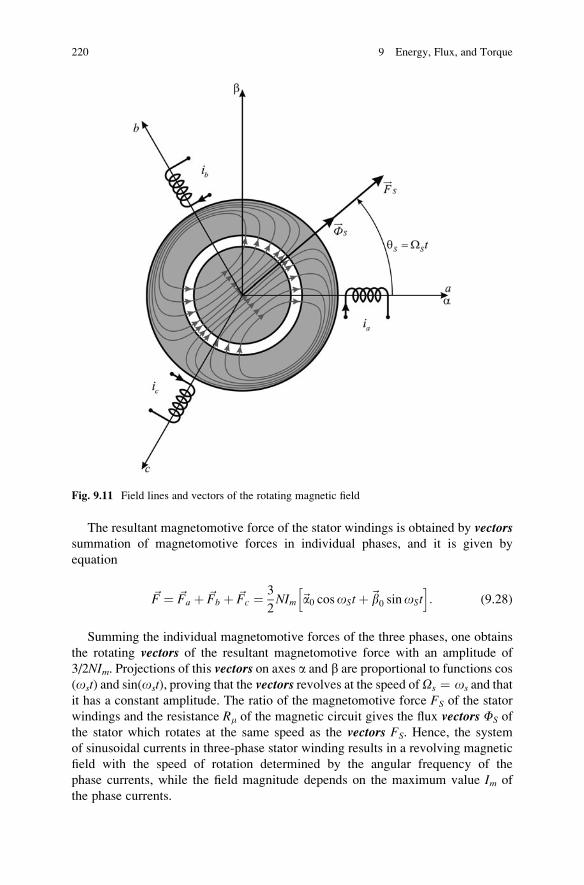
The resultant magnetomotive force of the stator windings is obtained by vectorssummation of magnetomotive forces in individual phases, and it is given by
equation
~F ¼ ~Fa þ ~Fb þ ~Fc ¼ 3
2NIm ~a0 cosoStþ~b0 sinoSt
h i: (9.28)
Summing the individual magnetomotive forces of the three phases, one obtains
the rotating vectors of the resultant magnetomotive force with an amplitude of
3/2NIm. Projections of this vectors on axes a and b are proportional to functions cos
(ost) and sin(ost), proving that the vectors revolves at the speed ofOs ¼ os and that
it has a constant amplitude. The ratio of the magnetomotive force FS of the stator
windings and the resistance Rm of the magnetic circuit gives the flux vectors FS of
the stator which rotates at the same speed as the vectors FS. Hence, the system
of sinusoidal currents in three-phase stator winding results in a revolving magnetic
field with the speed of rotation determined by the angular frequency of the
phase currents, while the field magnitude depends on the maximum value Im of
the phase currents.
Fig. 9.11 Field lines and vectors of the rotating magnetic field
220 9 Energy, Flux, and Torque
As already emphasized in the introduction, it is necessary to distinguish between
the speed of rotation of the rotor, being mechanical quantity expressed in rad/s, and
the angular frequency of electrical currents and voltages, appertaining to electrical
circuits and being expressed in rad/s as well. Throughout this book, mechanical
speed is denoted by O, while the angular frequency of voltages and currents is
denoted by o.Figure 9.11 shows vectors of the resultant magnetomotive force and the resultant
flux in electrical machine with three-phase system of stator windings.
9.9 Rotating Magnetic Field 221
Chapter 10
Electromotive Forces
Electromotive forces induced in windings of electrical machines are analyzed and
discussed in this chapter. Analysis includes transformer electromotive forces
and dynamic electromotive forces. The rms values, the waveforms, and harmonics
are derived for concentrated and distributed windings. For real windings that have
conductors distributed in a limited number of slots, the electromotive forces are
calculated by introducing, explaining, and using chord factors and belt factors.
Discussion includes design methods that suppress low-order harmonics in
electromotive forces. This chapter concludes with the analysis of distributed
windings with sinusoidal change of conductor density. Calculation of flux linkage
and electromotive force in such windings shows that they achieve suppression of all
harmonic distortions and operate as ideal spatial filters.
Variation of the flux in the machine windings results in induction of
electromotive forces, proportional to the first time derivative of the flux. The voltage
balance in each winding is given by equation u ¼ Ri + dC/dt, where u denotes thevoltage across the winding terminals, i is the electrical current in the winding, R is
the winding resistance, while the flux derivative represents the induced
electromotive force. In the introductory courses of electrical engineering,
the electromotive force is calculated as the first derivative of the flux with a leading
negative sign, e ¼ �dC/dt. This convention indicates that the induced electro-
motive force and consequential change in electrical current oppose to the flux
changes. Namely, in a short circuited winding (u ¼ 0), the flux changes produce
the electromotive force which, in turn, gives a rise to electrical current which
opposes to the flux changes. Adopting another convention has its own advantages
as well. By defining the electromotive force e ¼ +dC/dt, the current in the windingis determined as the ratio of the voltage difference (u � e) and the resistance R. Theelectromotive force defined as e ¼ +dC/dt is opposed to the voltage. Therefore, it isalso called counter electromotive force. In this book, the latter convention has beenadopted with e denoting +dC/dt and with the voltage balance in each windings beingu ¼ Ri + e.
S.N. Vukosavic, Electrical Machines, Power Electronics and Power Systems,
DOI 10.1007/978-1-4614-0400-2_10, # Springer Science+Business Media New York 2013
223
10.1 Transformer and Dynamic Electromotive Forces
Electromotive forces are generated due to changes of the winding flux. The flux can
change due to changes in electrical currents of the windings or due to motion of the
rotor with respect to the stator. In cases where the flux changes take place due to
motion, the consequential electromotive forces are called dynamic electromotiveforces. In cases where the stator windings carry constant currents, dynamic
electromotive force appears in the rotor winding which rotates with respect to
stator. Constant stator currents create a stationary magnetic field which does not
move with respect to the stator. One part of this flux encircles the rotor windings as
well. The rotor flux caused by the stator current depends on the relative position
between the stator and rotor. When the rotor moves, such rotor flux changes, and
this leads to creation of a dynamic electromotive force.
Electromotive force can also arise in cases with no rotor movement. If electrical
current in stator conductors is variable, the flux created by the stator winding is
variable as well. In part, the rotor flux is a consequence of stator currents. The
amount of the rotor flux caused by stator currents is determined by the mutual
inductance between the stator and rotor windings. Even with the rotor that does not
move, the rotor flux varies due to variable electrical currents in the stator winding.
As a consequence, an electromotive force is induced in the rotor winding. It is
called transformer electromotive force. In a power transformer, alternating currents
in the primary winding produce a variable flux which also encircles the secondary
winding. Variable flux leads to the transformer electromotive force in the second-
ary winding, providing the means for passing the electrical power from the primary
to the secondary side.
Electromotive force e ¼ Ldi/dt, which appears in a stand-alone winding due to
variation of the electrical current i, is proportional to the coefficient L, the self-
inductance of the winding. This electromotive force is called the electromotiveforce of self-induction.
10.2 Electromotive Force in One Turn
For the purpose of modeling electrical machines, it is necessary to calculate the
electromotive force induced in concentrated and distributed windings. Figure 10.1
shows an electrical machine with permanent magnets in the rotor magnetic circuit.
The magnets are shaped and arranged in the way to create sinusoidal distribution of
the magnetic induction in the air gap,
B ¼ Bm cosðy� ymÞ: (10.1)
Due to rotation of the rotor, the maximum induction Bm ¼ m0Hm is reached at
position y ¼ ym, where ym represents relative position of the rotor with respect to
224 10 Electromotive Forces
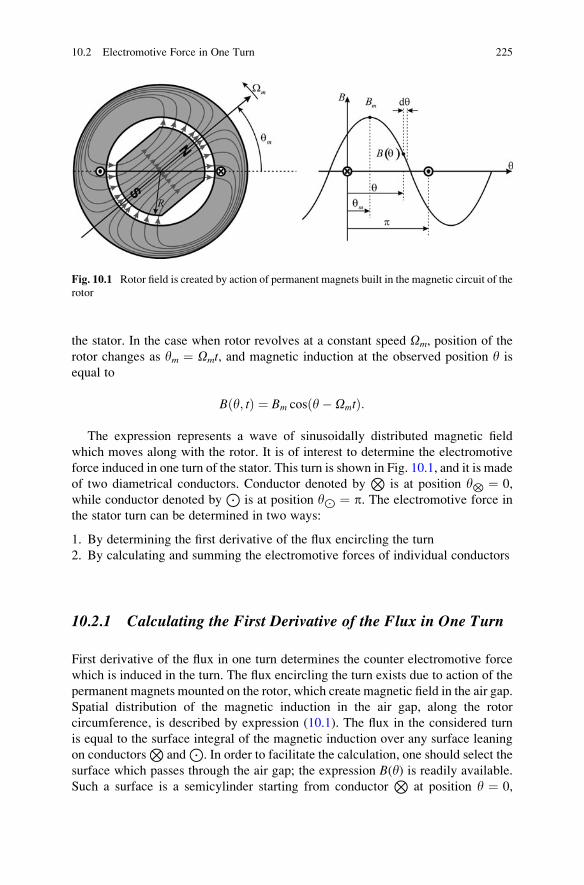
the stator. In the case when rotor revolves at a constant speed Om, position of the
rotor changes as ym ¼ Omt, and magnetic induction at the observed position y is
equal to
B y; tð Þ ¼ Bm cosðy� OmtÞ:
The expression represents a wave of sinusoidally distributed magnetic field
which moves along with the rotor. It is of interest to determine the electromotive
force induced in one turn of the stator. This turn is shown in Fig. 10.1, and it is made
of two diametrical conductors. Conductor denoted byN
is at position yN ¼ 0,
while conductor denoted byJ
is at position yJ ¼ p. The electromotive force in
the stator turn can be determined in two ways:
1. By determining the first derivative of the flux encircling the turn
2. By calculating and summing the electromotive forces of individual conductors
10.2.1 Calculating the First Derivative of the Flux in One Turn
First derivative of the flux in one turn determines the counter electromotive force
which is induced in the turn. The flux encircling the turn exists due to action of the
permanent magnets mounted on the rotor, which create magnetic field in the air gap.
Spatial distribution of the magnetic induction in the air gap, along the rotor
circumference, is described by expression (10.1). The flux in the considered turn
is equal to the surface integral of the magnetic induction over any surface leaning
on conductorsN
andJ
. In order to facilitate the calculation, one should select the
surface which passes through the air gap; the expression B(y) is readily available.
Such a surface is a semicylinder starting from conductorN
at position y ¼ 0,
Fig. 10.1 Rotor field is created by action of permanent magnets built in the magnetic circuit of the
rotor
10.2 Electromotive Force in One Turn 225
passing through the air gap in the upper part of the figure and ending up by leaning
on conductorJ
at position y ¼ p. The selected semicylinder has length L and
diameter R¸ where L is length and R is diameter of the rotor. Area of the selected
surface is
S ¼ L � R � p: (10.2)
The flux in the turn is calculated as the surface integral of the magnetic
induction, given by expression (10.1), over the selected surface, the semi cylinder.
Since the magnetic field in the air gap is radial, the vectors of the field H and the
magnetic induction B are perpendicular to the surface. The scalar product of vector
B and the surface element dS, the latter aided with the unit normal on the
semicylinder, becomes the product between the amplitudes of B and dS. Thus,the expression for the flux obtains the form
F ¼ðS
~B � d~S ¼ðS
B � dS:
Elementary surface of the semicylinder is dS ¼ L�R�dy, and expression for the
flux in one turn of the stator due to action of permanent magnets assumes the form
F ¼ðp
0
dF ¼ðp
0
B � dS ¼ðp
0
B � LRdy
¼ 2LRBmð Þ sin ym ¼ Fm sin ym: (10.3)
Flux in the turn is dependent on relative position between the stator and rotor.
Maximum value of the flux in one turn is reached when the rotor comes to position
y ¼ p/2. In this position, the flux is equal to Fm, where
Fm ¼ 2 � R � L � Bm: (10.4)
In other positions, the flux in one turn has smaller values, F(ym) ¼ Fmsinym.When the rotor revolves at a constant speed Om, the rotor position changes as
ym ¼ Omt, and the flux in one turn is
F ¼ Fm sin Omtð Þ;
while the (counter) electromotive force in the turn is
e1 ¼ þ dFdt
¼ OmFm cos Omtð Þ: (10.5)
226 10 Electromotive Forces
10.2.2 Summing Electromotive Forces of Individual Conductors
It is possible to determine the electromotive force in one turn by summing the
electromotive forces of individual conductors that make one turn. In the example
presented in Fig. 10.1, the field of permanent magnets revolves with respect to
the stator conductors. The peripheral speed of relative motion is v ¼ ROm, where Ris the rotor radius and Om is the angular speed of the rotor. In the conductor denoted
byN
, the electromotive force is
e� ¼ L � R � Om � Bm � cos Omtð Þ:
At position y ¼ p, where the diametrical conductorJ
is placed, the magnetic
induction has the same amplitude and the opposite direction. For this reason, the
electromotive force eJ induced in the conductor denoted byJ
is of the opposite
direction, eN ¼ �eJ. The electromotive force in one turn is obtained by summing
the electromotive forces in individual conductors. One turn is formed by connecting
the two conductors in series. The terminals of the turn are made available at the
front side of the cylinder. The other ends of the conductorsN
andJ
are connected
at the rear side of the cylinder. Therefore, when circulating along the contour made
by the two conductors, the electromotive forces of conductors eN and eJ are
summed according to e ¼ eN � eJ. Finally, the electromotive force in one turn is
e1 ¼ 2 � e� ¼ 2 � L � R � Om � Bm � cos Omtð Þ: (10.6)
According to expression (10.4), the maximum value of the flux in one turn is
equal to Fm ¼ 2LRBm, and the previous expression can be written as
e1 ¼ OmFm cos Omtð Þ; (10.7)
which is in accordance with (10.5).
In the considered example, the induced electromotive forces are harmonic
functions of time; thus, it is possible to represent them by phasors. Summing the
electromotive forces eN and eJ can be represented by phasors, as shown in
Fig. 10.3.
10.2.3 Voltage Balance in One Turn
The voltage balance within one turn is given by equation
u ¼ Riþ e1 � dFdt
¼ 2OmLRBm cos ym
¼ OmFm cos ym ¼ Em cos ym ; (10.8)
10.2 Electromotive Force in One Turn 227
where e1 represents (counter) electromotive force. If the resistance R of the turn is
sufficiently low, the voltage drop Ri can be neglected, and the electromotive force
e1 is equal to the voltage across the terminals of the turn. Since the electromotive
force is a sinusoidal function of time, its rms (root mean square) value is given by
(10.9), where f is the frequency in Hz, that is, the number of rotor revolutions per
second. Therefore, the electromotive force is proportional to the maximum value of
the flux and to the frequency,
Eturn1rms ¼
Emffiffiffi2
p ¼ 2pfð ÞFmffiffiffi2
p ¼ 4; 44f Fm: (10.9)
10.2.4 Electromotive Force Waveform
Preceding analysis dealt with an electrical machine with permanent magnets on the
rotor which create magnetic field with sinusoidal distribution B(y) along the air gapcircumference. With constant rotor speed, sinusoidal electromotive force is induced
in stator turn shown in Fig. 10.1.
If the speed of rotation varies, the electromotive force induced in the turn may
deviate from sinusoidal change. In cases when distribution of magnetic field is
sinusoidal, but the speed of rotation changes in time, Om(t), the electromotive force
in the turn is
e1 ¼ þ d
dtFm sin Omtð Þð Þ
¼ OmFm cos Omtð Þ þ t � Fm cos Omtð Þ � dOm
dt:
This expression represents a harmonic function of time if the speed of rotation is
constant, that is, in cases where dOm/dt ¼ 0.
In cases where the permanent magnets create a non-sinusoidal periodic distribu-
tion of the magnetic field in the air gap, the induced electromotive force assumes a
non-sinusoidal function of time. Let B(y � ym) be a periodic function specifying
the change of the magnetic induction along the air gap circumference. At position
of the conductorN
, magnetic induction is equal to BN ¼ B(0 � ym) ¼ B(�ym).If the rotor revolves at a constant speed, the electromotive force of the turn
calculated according to expression (10.6) is equal to
e1 ¼ 2 � e� ¼ 2LROm � B� ¼ 2LROm � B �Omtð Þ: (10.10)
The obtained expression shows that the electromotive force waveform is deter-
mined by the function B(y � ym), expressing the spatial distribution of the mag-
netic induction originating from the rotor permanent magnets. Therefore, the form
228 10 Electromotive Forces

of the function B(y � ym) determines the waveform e1(t) of the electromotive force
in one turn. In cases with non-sinusoidal distribution B(y � ym) of the magnetic
field in the air gap, the electromotive force induced in the turn (Fig. 10.1) will be
non-sinusoidal as well.
Question (10.1): Assume that synchronous generator supplies electrical loads and
comprises concentrated stator winding with all the conductors located in two slots
on the inner surface of the stator. These slots are diametrically positioned grooves in
the magnetic circuit facing the air gap. Permanent magnets of the rotor create the
induction B(y) ¼ Bm sgn[cos(y � ym)] in the air gap. Determine and sketch the
form of the voltage supplied to the electrical load.
Answer (10.1): In accordance with (10.8), the voltage across terminals of the
stator winding is equal to
u � 2NLROmB Omtð Þ ¼ 2NLROmBmð Þ sgn cos Omtð Þ½ �:
10.2.5 Root Mean Square (rms) Value of Electromotive Forces
The AC voltages and currents in electrical engineering are characterized by their
rms value (root mean square). Sinusoidal voltages and currents are mostly
described in terms of their rms value instead of their peak values. Root mean square(rms) value of an AC voltage corresponds to DC voltage that would result in the
same power when applied to resistive loads. Namely, when an AC voltage with
the rms value of U is applied to the resistance R, the power dissipated in resistive
load will be P ¼ U2/R. The same power is obtained when a DC voltageU is applied
across the same resistance. Therefore, the rms value of AC voltages is also called
equivalent DC voltage. For sinusoidal voltages, their rms value is obtained by
dividing their peak value by the square root of two. The rms value can be defined
as well for periodic non-sinusoidal voltages. For a voltage that changes periodically
with a period T, the rms value is calculated according to
Urms ¼
ffiffiffiffiffiffiffiffiffiffiffiffiffiffiffiffi1
T
ðT
0
u2dt
vuuut :
The rms value can be also defined for AC currents, using the previous expression.
For sinusoidal currents, their rms value is √2 times lower than their peak value.
Expressions (10.11) and (10.12) give the rms value of the electromotive force in one
turn and rms value of the electromotive force in one conductor,
Eturn1rms ¼
Emffiffiffi2
p ¼ 2pfð ÞFmffiffiffi2
p ¼ 4; 44f Fm (10.11)
10.2 Electromotive Force in One Turn 229
Econ1rms ¼ 2; 22f Fm: (10.12)
The angular frequency o ¼ 2pf of the electromotive force is determined by the
speed of rotation Om. The rms value of an induced electromotive force can be
expressed in terms of the frequency f and the flux as Erms ¼ 4.44 fFm. For a
concentrated winding consisting of N turns, the rms value of the electromotive
force is given by equation
Ewindrms ¼ 4; 44Nf Fm: (10.13)
10.3 Electromotive Force in a Winding
Electrical machines usually have a number of windings. Most induction and
synchronous machines, also called AC machines, have their stator designed for
the connection to a three-phase system of alternating voltages and currents. There-
fore, most AC machines have three windings on the stator, also called phase
windings. Some authors use the term stator winding to describe the winding systemcomprising three-phase windings.
Each winding has one or more turns. Individual turns are connected in series.
The ends of this series connection are usually made available at machine terminals.
In this section, the electromotive force induced in a winding is calculated for
concentrated and distributed windings. This electromotive force determines the
voltage across the machine terminals.
10.3.1 Concentrated Winding
Conductors making a winding can be concentrated in two diametrically positioned
grooves, constituting a concentrated winding. Since all the turns of a concentrated
winding reside in the same position, they all have the same flux and the same
electromotive force. The rms value of the electromotive force in one turn, made of
two diametrically positioned conductors, is given by expression (10.12). For a
concentrated winding with N turns, the rms value of the induced electromotive
force is given by expression (10.14).
10.3.2 Distributed Winding
Windings are usually made by placing conductors in a number of equally spaced
slots along the machine circumference. Individual turns are spatially shifted and
have different electromotive forces. For this reason, the electromotive force
230 10 Electromotive Forces
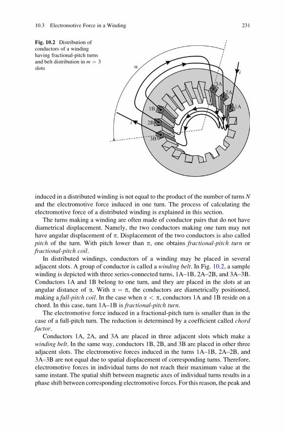
induced in a distributed winding is not equal to the product of the number of turns Nand the electromotive force induced in one turn. The process of calculating the
electromotive force of a distributed winding is explained in this section.
The turns making a winding are often made of conductor pairs that do not have
diametrical displacement. Namely, the two conductors making one turn may not
have angular displacement of p. Displacement of the two conductors is also called
pitch of the turn. With pitch lower than p, one obtains fractional-pitch turn or
fractional-pitch coil.In distributed windings, conductors of a winding may be placed in several
adjacent slots. A group of conductor is called a winding belt. In Fig. 10.2, a sample
winding is depicted with three series-connected turns, 1A–1B, 2A–2B, and 3A–3B.
Conductors 1A and 1B belong to one turn, and they are placed in the slots at an
angular distance of a. With a ¼ p, the conductors are diametrically positioned,
making a full-pitch coil. In the case when a < p, conductors 1A and 1B reside on a
chord. In this case, turn 1A–1B is fractional-pitch turn.The electromotive force induced in a fractional-pitch turn is smaller than in the
case of a full-pitch turn. The reduction is determined by a coefficient called chordfactor.
Conductors 1A, 2A, and 3A are placed in three adjacent slots which make a
winding belt. In the same way, conductors 1B, 2B, and 3B are placed in other three
adjacent slots. The electromotive forces induced in the turns 1A–1B, 2A–2B, and
3A–3B are not equal due to spatial displacement of corresponding turns. Therefore,
electromotive forces in individual turns do not reach their maximum value at the
same instant. The spatial shift between magnetic axes of individual turns results in a
phase shift between corresponding electromotive forces. For this reason, the peak and
Fig. 10.2 Distribution of
conductors of a winding
having fractional-pitch turns
and belt distribution in m ¼ 3
slots
10.3 Electromotive Force in a Winding 231
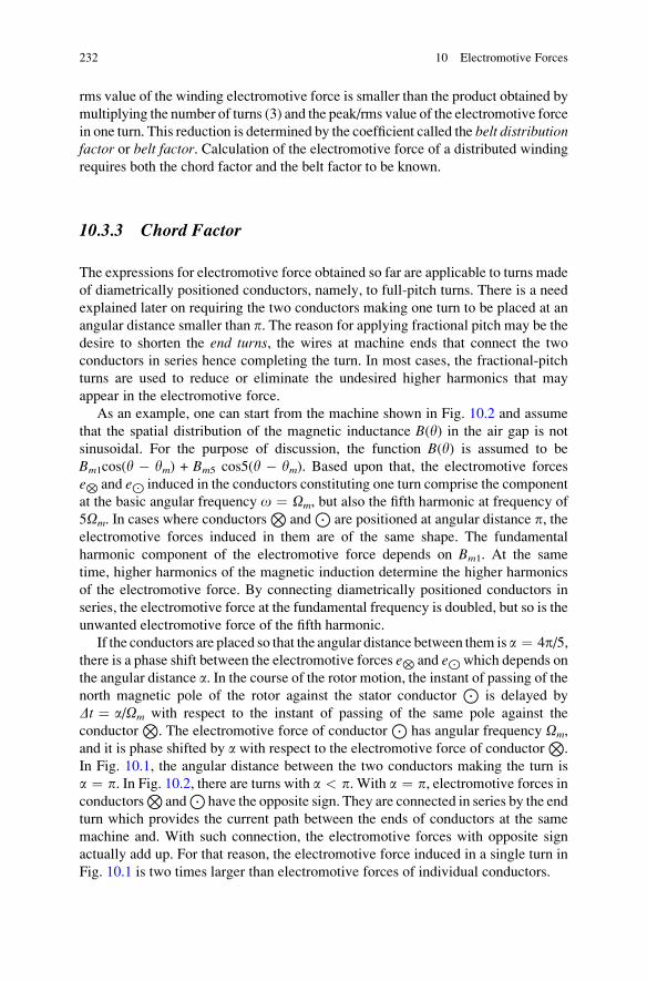
rms value of the winding electromotive force is smaller than the product obtained by
multiplying the number of turns (3) and the peak/rms value of the electromotive force
in one turn. This reduction is determined by the coefficient called the belt distributionfactor or belt factor. Calculation of the electromotive force of a distributed winding
requires both the chord factor and the belt factor to be known.
10.3.3 Chord Factor
The expressions for electromotive force obtained so far are applicable to turns made
of diametrically positioned conductors, namely, to full-pitch turns. There is a need
explained later on requiring the two conductors making one turn to be placed at an
angular distance smaller than p. The reason for applying fractional pitch may be the
desire to shorten the end turns, the wires at machine ends that connect the two
conductors in series hence completing the turn. In most cases, the fractional-pitch
turns are used to reduce or eliminate the undesired higher harmonics that may
appear in the electromotive force.
As an example, one can start from the machine shown in Fig. 10.2 and assume
that the spatial distribution of the magnetic inductance B(y) in the air gap is not
sinusoidal. For the purpose of discussion, the function B(y) is assumed to be
Bm1cos(y � ym) + Bm5 cos5(y � ym). Based upon that, the electromotive forces
eN and eJ induced in the conductors constituting one turn comprise the component
at the basic angular frequency o ¼ Om, but also the fifth harmonic at frequency of
5Om. In cases where conductorsN
andJ
are positioned at angular distance p, theelectromotive forces induced in them are of the same shape. The fundamental
harmonic component of the electromotive force depends on Bm1. At the same
time, higher harmonics of the magnetic induction determine the higher harmonics
of the electromotive force. By connecting diametrically positioned conductors in
series, the electromotive force at the fundamental frequency is doubled, but so is the
unwanted electromotive force of the fifth harmonic.
If the conductors are placed so that the angular distance between them is a ¼ 4p/5,there is a phase shift between the electromotive forces eN and eJwhich depends on
the angular distance a. In the course of the rotor motion, the instant of passing of the
north magnetic pole of the rotor against the stator conductorJ
is delayed by
Dt ¼ a/Om with respect to the instant of passing of the same pole against the
conductorN
. The electromotive force of conductorJ
has angular frequency Om,
and it is phase shifted by a with respect to the electromotive force of conductorN
.
In Fig. 10.1, the angular distance between the two conductors making the turn is
a ¼ p. In Fig. 10.2, there are turns with a < p. With a ¼ p, electromotive forces in
conductorsN
andJ
have the opposite sign. They are connected in series by the end
turn which provides the current path between the ends of conductors at the same
machine and. With such connection, the electromotive forces with opposite sign
actually add up. For that reason, the electromotive force induced in a single turn in
Fig. 10.1 is two times larger than electromotive forces of individual conductors.
232 10 Electromotive Forces
Electromotive forces in individual conductors can be represented by phasors
eN and eJ. With peripheral rotor speed of v ¼ ROm, and with B(y) ¼ Bm
cos(y � ym), both phasors have the same amplitude |eN| ¼ |eJ| ¼ e1 ¼ LvBm,
where L denotes the axial length of the machine. The phasor of the electromotive
force in the turn, shown in Fig. 10.3a, is obtained by summing the phasors eN and
eJ, e ¼ eN � eJ. With angular distance between conductors of a, eN ¼ e1, eJ
¼ e1e�ja and (-eJ) ¼ e1e
�ja+jp. By placing the conductors at angular distance 4p/5,phasors of electromotive forces eN and eJ are not be collinear, and this is illustrated
in part (b) of Fig. 10.3.With respect to eN, electromotive force�eJ is phase shifted
by p/5. Therefore, the amplitude of the resulting electromotive force in one turn
eN � eJ is slightly smaller than the sum of amplitudes LvBm of electromotive
forces in individual conductors.
Phasor diagrams can be constructed for the fundamental harmonic but also for
each of the higher harmonics. With B(y) ¼ Bm1cos(y � ym) + Bm5 cos5(y � ym),electromotive forces have the fundamental component of frequency Om and ampli-
tude determined by Bm1 and the fifth harmonic of frequency 5Om and amplitude
determined by Bm5. For the fifth harmonic of electromotive forces, the phase
difference is multiplied by 5, as well as the frequency. Since 5 � p/5 ¼ p, thefifth harmonic of the electromotive force eN is in opposition with the fifth harmonic
of the electromotive force (�eJ). Thus, they will be mutually canceled. Despite the
presence of the fifth harmonic in the spatial distribution of B(y), the electromotive
force induced in the considered turn will not contain the fifth harmonic. One of the
consequences of shortening the turn pitch is reduction of the first, fundamental
harmonic of the electromotive force. The electromotive force in one turn formed by
the fractional-pitch conductors can be determined from the phasor diagrams of
Fig. 10.3 Electromotive forces of conductors of a turn. (a) Full-pitched turn. (b) Fractional-pitch
turn
10.3 Electromotive Force in a Winding 233
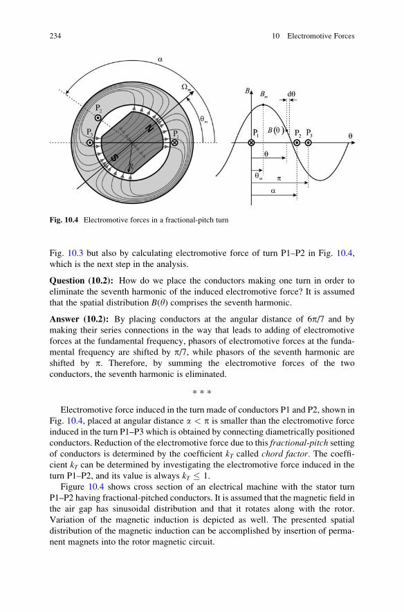
Fig. 10.3 but also by calculating electromotive force of turn P1–P2 in Fig. 10.4,
which is the next step in the analysis.
Question (10.2): How do we place the conductors making one turn in order to
eliminate the seventh harmonic of the induced electromotive force? It is assumed
that the spatial distribution B(y) comprises the seventh harmonic.
Answer (10.2): By placing conductors at the angular distance of 6p/7 and by
making their series connections in the way that leads to adding of electromotive
forces at the fundamental frequency, phasors of electromotive forces at the funda-
mental frequency are shifted by p/7, while phasors of the seventh harmonic are
shifted by p. Therefore, by summing the electromotive forces of the two
conductors, the seventh harmonic is eliminated.
* * *
Electromotive force induced in the turn made of conductors P1 and P2, shown in
Fig. 10.4, placed at angular distance a < p is smaller than the electromotive force
induced in the turn P1–P3 which is obtained by connecting diametrically positioned
conductors. Reduction of the electromotive force due to this fractional-pitch settingof conductors is determined by the coefficient kT called chord factor. The coeffi-
cient kT can be determined by investigating the electromotive force induced in the
turn P1–P2, and its value is always kT � 1.
Figure 10.4 shows cross section of an electrical machine with the stator turn
P1–P2 having fractional-pitched conductors. It is assumed that the magnetic field in
the air gap has sinusoidal distribution and that it rotates along with the rotor.
Variation of the magnetic induction is depicted as well. The presented spatial
distribution of the magnetic induction can be accomplished by insertion of perma-
nent magnets into the rotor magnetic circuit.
Fig. 10.4 Electromotive forces in a fractional-pitch turn
234 10 Electromotive Forces
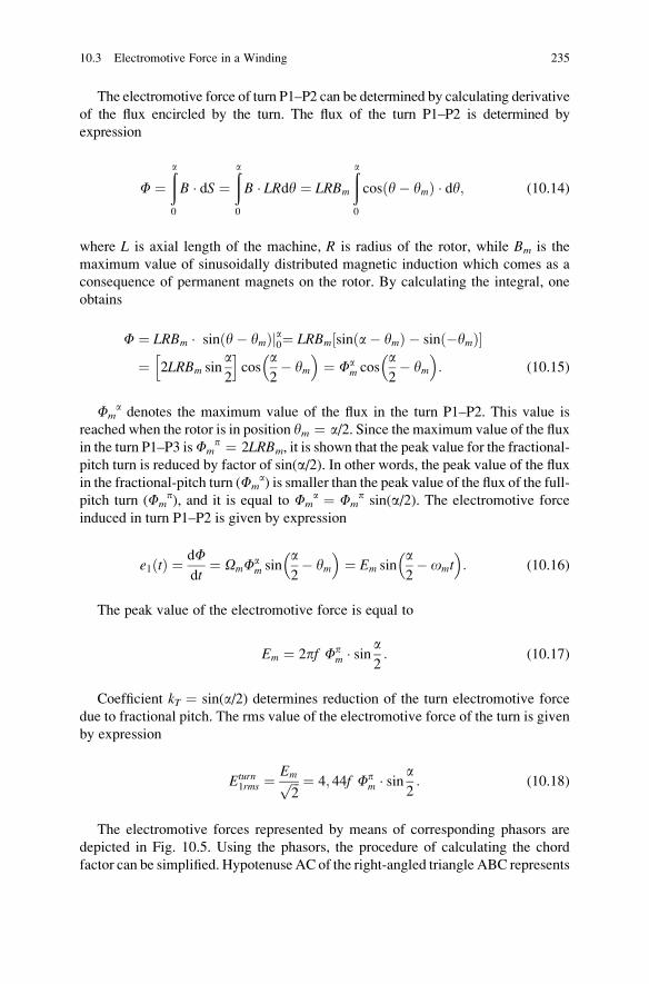
The electromotive force of turn P1–P2 can be determined by calculating derivative
of the flux encircled by the turn. The flux of the turn P1–P2 is determined by
expression
F ¼ða
0
B � dS ¼ða
0
B � LRdy ¼ LRBm
ða
0
cos y� ymð Þ � dy; (10.14)
where L is axial length of the machine, R is radius of the rotor, while Bm is the
maximum value of sinusoidally distributed magnetic induction which comes as a
consequence of permanent magnets on the rotor. By calculating the integral, one
obtains
F ¼ LRBm � sin y� ymð Þja0¼ LRBm sinða� ymÞ � sinð�ymÞ½ �¼ 2LRBm sin
a2
h icos
a2� ym
� �¼ Fa
m cosa2� ym
� �: (10.15)
Fma denotes the maximum value of the flux in the turn P1–P2. This value is
reached when the rotor is in position ym ¼ a/2. Since the maximum value of the flux
in the turn P1–P3 isFmp ¼ 2LRBm, it is shown that the peak value for the fractional-
pitch turn is reduced by factor of sin(a/2). In other words, the peak value of the fluxin the fractional-pitch turn (Fm
a) is smaller than the peak value of the flux of the full-
pitch turn (Fmp), and it is equal to Fm
a ¼ Fmp sin(a/2). The electromotive force
induced in turn P1–P2 is given by expression
e1ðtÞ ¼ dFdt
¼ OmFam sin
a2� ym
� �¼ Em sin
a2� omt
� �: (10.16)
The peak value of the electromotive force is equal to
Em ¼ 2pf Fpm � sin a
2: (10.17)
Coefficient kT ¼ sin(a/2) determines reduction of the turn electromotive force
due to fractional pitch. The rms value of the electromotive force of the turn is given
by expression
Eturn1rms ¼
Emffiffiffi2
p ¼ 4; 44f Fpm � sin a
2: (10.18)
The electromotive forces represented by means of corresponding phasors are
depicted in Fig. 10.5. Using the phasors, the procedure of calculating the chord
factor can be simplified. Hypotenuse AC of the right-angled triangle ABC represents
10.3 Electromotive Force in a Winding 235
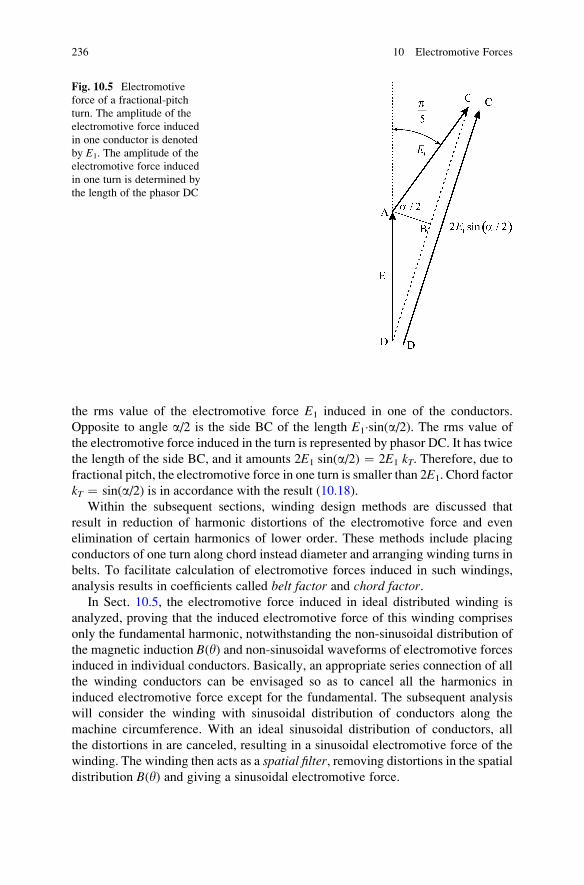
the rms value of the electromotive force E1 induced in one of the conductors.
Opposite to angle a/2 is the side BC of the length E1�sin(a/2). The rms value of
the electromotive force induced in the turn is represented by phasor DC. It has twice
the length of the side BC, and it amounts 2E1 sin(a/2) ¼ 2E1 kT. Therefore, due tofractional pitch, the electromotive force in one turn is smaller than 2E1. Chord factor
kT ¼ sin(a/2) is in accordance with the result (10.18).
Within the subsequent sections, winding design methods are discussed that
result in reduction of harmonic distortions of the electromotive force and even
elimination of certain harmonics of lower order. These methods include placing
conductors of one turn along chord instead diameter and arranging winding turns in
belts. To facilitate calculation of electromotive forces induced in such windings,
analysis results in coefficients called belt factor and chord factor.In Sect. 10.5, the electromotive force induced in ideal distributed winding is
analyzed, proving that the induced electromotive force of this winding comprises
only the fundamental harmonic, notwithstanding the non-sinusoidal distribution of
the magnetic induction B(y) and non-sinusoidal waveforms of electromotive forces
induced in individual conductors. Basically, an appropriate series connection of all
the winding conductors can be envisaged so as to cancel all the harmonics in
induced electromotive force except for the fundamental. The subsequent analysis
will consider the winding with sinusoidal distribution of conductors along the
machine circumference. With an ideal sinusoidal distribution of conductors, all
the distortions in are canceled, resulting in a sinusoidal electromotive force of the
winding. The winding then acts as a spatial filter, removing distortions in the spatial
distribution B(y) and giving a sinusoidal electromotive force.
Fig. 10.5 Electromotive
force of a fractional-pitch
turn. The amplitude of the
electromotive force induced
in one conductor is denoted
by E1. The amplitude of the
electromotive force induced
in one turn is determined by
the length of the phasor DC
236 10 Electromotive Forces
10.3.4 Belt Factor
Windings of practical machines are made by placing conductors in slots, axially cut
grooves in the magnetic circuit. The stator and rotor have large numbers of slots.
Figure 8.1 shows a cross section of the magnetic circuit of an electrical machine
exposing the usual shapes of the slots and their number.
One turn consists of the two diametrical conductors or the two conductors placed
at the ends of the chord. On the other hand, a three-phase stator winding comprises
three phases, three separate windings having their magnetic axes displaced by 2p/3.Therefore, the minimum number of slots contained by the stator magnetic circuit of
a three-phase machine is 2 � 3 ¼ 6. This number of slots is used in cases where
each of the phase windings is concentrated, that is, where all conductors in a
winding are placed in two diametrical slots. The number of slots is usually higher
than 6. One of the reasons for using higher number of slots is the problem associated
with placing one half of all the conductors of one winding into only one slot. Such
slot would have an extremely large cross section that is not practical for the
machine construction. Thus, the conductors are usually distributed in a number of
neighboring slots. In this way, a winding belt is formed. A belt comprises two, three,
or more adjacent slots. Each slot of the belt can accommodate one or more winding
conductors. In order to simplify further considerations, one may assume that
each slot of the belt contains only one conductor. In cases where each slot has Mconductors, all the subsequent conclusions hold, except for the electromotive forces
amplitude which has to be multiplied by M.
An example of a winding belt having conductors placed in three adjacent slots is
presented in Fig. 10.6 The figure shows the cross section of such winding and
phasor diagram showing relation between the electromotive forces induced in the
individual windings. The turns 1A–1B, 2A–2B, and 3A–3B have full pitch, namely,
these turns are made of diametrically positioned conductors. Phasors E1, E2, and E3
represent the electromotive forces of turns 1A–1B, 2A–2B, and 3A–3B, respec-
tively. Angle g in Fig. 10.6 denotes the distance between the two adjacent slots. Thespatial shift between the turns results in the phase shift g between electromotive
forces induced in corresponding turns.
Placing of conductors in winding belts allows elimination or reduction of higher
harmonics in the induced electromotive force. Due to the spatial displacement
between conductors, the electromotive forces in individual conductors are phase
shifted, as explained in the preceding section discussing the chord factor. In cases
where a winding belt ranges over m neighboring slots, the electromotive force of
the winding can be determined according to equation
~Ephase ¼ ~E1 þ ~E2 þ :::þ ~Em; (10.19)
where letters E1Em denote the electromotive forces induced in individual turns.
Due to the phase shift, the sum of individual electromotive forces gives a resultant
10.3 Electromotive Force in a Winding 237
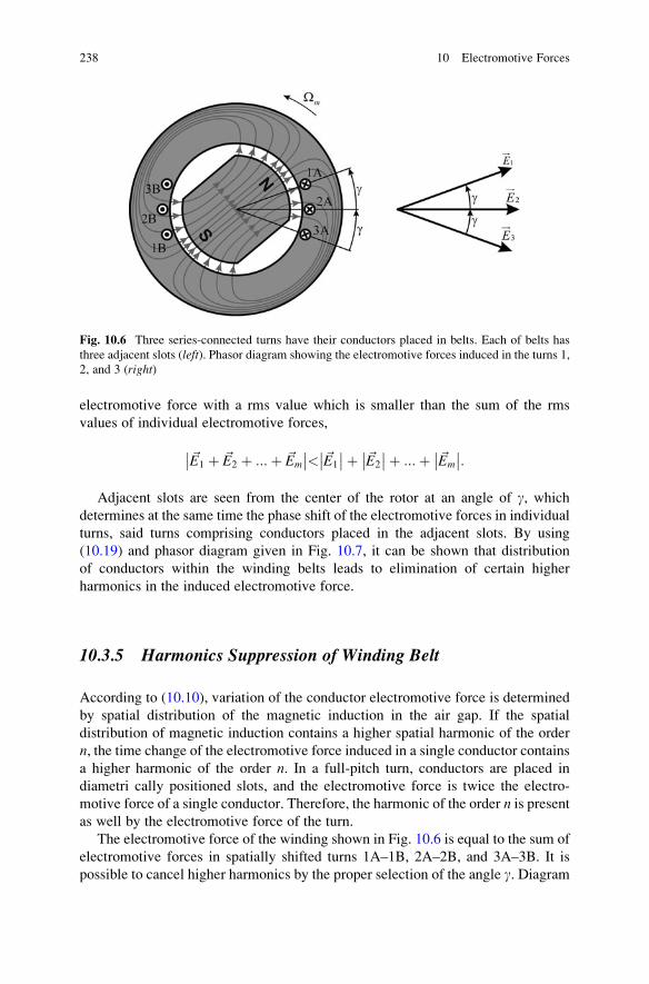
electromotive force with a rms value which is smaller than the sum of the rms
values of individual electromotive forces,
~E1 þ ~E2 þ :::þ ~Em
�� ��< ~E1
�� ��þ ~E2
�� ��þ :::þ ~Em
�� ��:Adjacent slots are seen from the center of the rotor at an angle of g, which
determines at the same time the phase shift of the electromotive forces in individual
turns, said turns comprising conductors placed in the adjacent slots. By using
(10.19) and phasor diagram given in Fig. 10.7, it can be shown that distribution
of conductors within the winding belts leads to elimination of certain higher
harmonics in the induced electromotive force.
10.3.5 Harmonics Suppression of Winding Belt
According to (10.10), variation of the conductor electromotive force is determined
by spatial distribution of the magnetic induction in the air gap. If the spatial
distribution of magnetic induction contains a higher spatial harmonic of the order
n, the time change of the electromotive force induced in a single conductor contains
a higher harmonic of the order n. In a full-pitch turn, conductors are placed in
diametri cally positioned slots, and the electromotive force is twice the electro-
motive force of a single conductor. Therefore, the harmonic of the order n is presentas well by the electromotive force of the turn.
The electromotive force of the winding shown in Fig. 10.6 is equal to the sum of
electromotive forces in spatially shifted turns 1A–1B, 2A–2B, and 3A–3B. It is
possible to cancel higher harmonics by the proper selection of the angle g. Diagram
Fig. 10.6 Three series-connected turns have their conductors placed in belts. Each of belts has
three adjacent slots (left). Phasor diagram showing the electromotive forces induced in the turns 1,
2, and 3 (right)
238 10 Electromotive Forces
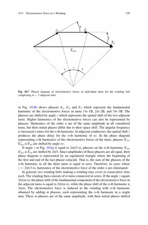
in Fig. 10.6b shows phasors E1, E2, and E3 which represent the fundamental
harmonic of the electromotive forces in turns 1A–1B, 2A–2B, and 3A–3B. The
phasors are shifted by angle g which represents the spatial shift of the two adjacent
turns. Higher harmonics of the electromotive forces can also be represented by
phasors. Harmonics of the order n are of the same amplitude in all considered
turns, but their initial phases differ due to their space shift. The angular frequency
is increased n times for the n-th harmonic. In adjacent conductors, the spatial shift gproduces the phase delay for the n-th harmonic of ng. In the phase diagram
representing n-th harmonics of the electromotive forces of the turns, phasors Е1n,
Е2n, и Е3n are shifted by angle ng.If angle g in Fig. 10.6a is equal to 2p/(3�n), phasors on the n-th harmonic Е1n,
Е2n, и Е3n are shifted by 2p/3. Since amplitudes of these phasors are all equal, their
phase diagram is represented by an equilateral triangle where the beginning of
the first and end of the last phasor coincide. That is, the sum of the phasors of the
n-th harmonic in all the three turns is equal to zero. Therefore, in cases where
g ¼ 2p/(3�n), harmonics of the electromotive force of the order n are eliminated.
In general, two winding belts making a winding may cover m consecutive slots
each. The winding then consists of m turns connected in series. If the angle g equals2p/(m�n), the phase shift of the fundamental component of the electromotive force in
the adjacent turns is equal to 2p/(m�n), while the phase shift of the n-th harmonic is
2p/m. The electromotive force is induced in the winding with n-th harmonic
obtained by adding m phasors, each representing the n-th harmonic in a single
turn. These m phasors are of the same amplitude, with their initial phases shifted
Fig. 10.7 Phasor diagram of electromotive forces in individual turns for the winding belt
comprising m ¼ 3 adjacent slots
10.3 Electromotive Force in a Winding 239
by 2p/m. The phasor representing the n-th harmonic of the electromotive force of the
winding comprising m series-connected turns is
Ewindn ¼ E1n þ E2n þ E3n þ :::þ Emn
¼ E1n
Xm�1
k¼0
e�j�k�2pm ¼ 0:
The last expression can be represented graphically. By addingm phasors mutually
shifted by 2p/m, the end of the last phasor coincides with the beginning of the first
one. The phasor diagram is represented by a polygon of m sides of equal length. The
polygon is inscribed within the circle with phasors of the n-th harmonic in individual
turns being the chords of the circle.
Therefrom, one can conclude that the resultant electromotive force of the
harmonic of the n-th order is equal to zero provided that the angle g equals
2p/(m�n). In other words, the n-th harmonic can be eliminated provided that the
winding belt spans over m slots is placed at an angular distance of 2p/n.With the slots distributed in a belt, the fundamental component of the resultant
electromotive force is slightly smaller than what would be the electromotive force
in a concentrated winding. By using the diagram in Fig. 10.7, it can be noticed that
the amplitude of the sum of phasors E1 þ E2 þ E3 is smaller than the sum of
individual amplitudes |E1| þ |E2| þ |E3|. This difference appears since the phasors
being added are not collinear. Factor kP is equal to the ratio
kP ¼~E1 þ ~E2 þ ~E3
�� ��~E1
�� ��þ ~E2
�� ��þ ~E3
�� ��and it is called belt factor.
In cases where the width of the winding belt is m ¼ 3, the fundamental compo-
nent of the resultant electromotive force is obtained by adding three phasors, as
shown in Fig. 10.7, resulting in equation
~Ewindm¼3 ¼ ~E1 þ ~E2 þ ~E3: (10.20)
Phasors E1, E2, and E3 are lying on a circle of radius R. For each of the isoscelestriangles of Fig. 10.7, it is known that the base of the triangle is equal to twice the
product of the triangle side and the sine of one half of the opposite angle. Therefore,
the expression R sin(g/2) ¼ E1/2 links the radius of the circle, the electromotive
force E1, and the angle g. At the same time, the amplitude of the resultant phasor is
Em¼3 ¼ 2R � sin 3g2¼ 2
E1
2 � sin g2
� �sin
3g2
¼ E1
sin 3g2
sin g2
¼ sin 3g2
3 � sin g2
!� 3E1 ¼ kP � 3E1;
240 10 Electromotive Forces
where kP stands for the belt factor of the winding with the belt width ofm ¼ 3 slots.
For belt width m 6¼ 3, the amplitude of the resultant phasor representing the
fundamental harmonic component is Em ¼ 2R sin(mg/2), where radius R and
electromotive force E1 in one turn are related by R sin(g/2) ¼ E1/2. With E1
representing the rms value of the fundamental component of the electromotive
force induced in a single turn, the rms value of the fundamental component in the
winding comprising m series-connected turns is
Em ¼ E1
sin mg2
sin g2
¼ sin mg2
m � sin g2
� �� mE1 ¼ kP � mE1:
The belt factor kP is determined by the expression
kP ¼~Em¼3
�� ��m ~E1
�� �� ¼sin mg
2
m � sin g2
; (10.21)
and the rms value of the winding electromotive force can be determined from
Erms ¼ Ephase ¼ 4; 44kPfN Fpm; (10.22)
where Fmp ¼ 2LRBm is the maximum value of the flux in one full-pitched turn, N is
the number of series-connected turns, while f ¼ Om/(2p) is the frequency.
Question (10.3): Due to non-sinusoidal distribution of magnetic induction B(y),the electromotive forces induced in conductors comprise higher harmonics. A
winding of 3 turns consists of 6 conductors. The conductors are placed at angular
distance of g ¼ 24. The resultant electromotive force measured at the winding
terminals does not have some of the higher harmonics that are present in
electromotive forces of single conductor. What is the order of these harmonics?
Answer (10.3): The resultant electromotive force of the harmonic of the order n isequal to zero in cases where g ¼ 2p/(m�n) or g ¼ q�2p/(m�n), where q is an integer.Since m ¼ 3 and g ¼ 2p/15, all harmonics of the order n ¼ 5q are eliminated.
These are all the harmonics with the order n being an integer multiple of five.
10.4 Electromotive Force of Compound Winding
Windings are usually made by series connecting the fractional-pitch turns, namely,
the turns made of conductors that are not diametrically placed, but reside at the ends
of a chord. In addition, conductors of several turns are distributed in adjacent slots
that make up one winding belt. For this reason, calculation of the fundamental (first)
harmonic component in the electromotive force of the winding should include the
belt and pitch factors. These factors are given by expressions
10.4 Electromotive Force of Compound Winding 241
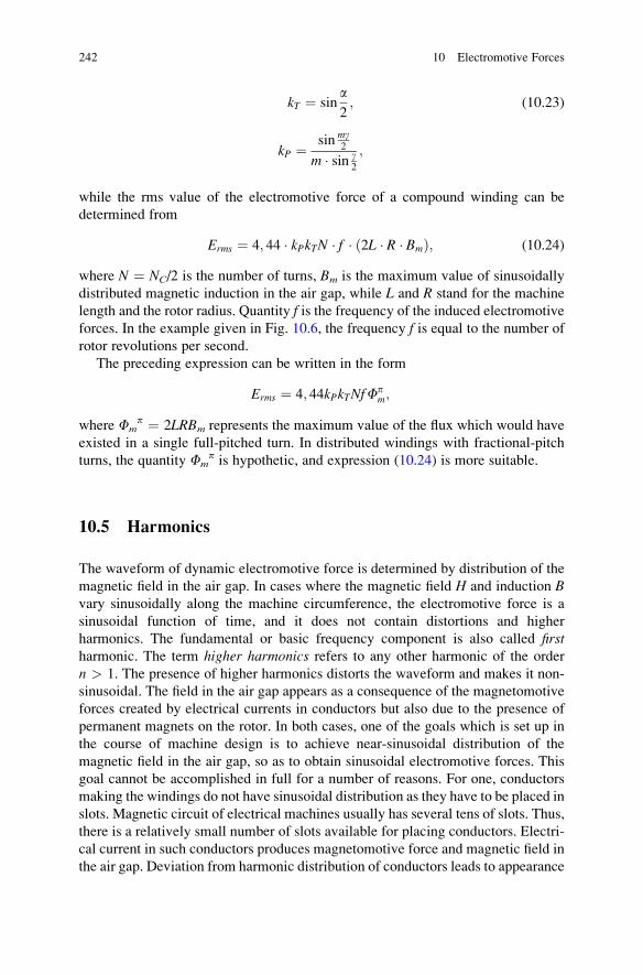
kT ¼ sina2; (10.23)
kP ¼ sin mg2
m � sin g2
;
while the rms value of the electromotive force of a compound winding can be
determined from
Erms ¼ 4; 44 � kPkTN � f � 2L � R � Bmð Þ; (10.24)
where N ¼ NC/2 is the number of turns, Bm is the maximum value of sinusoidally
distributed magnetic induction in the air gap, while L and R stand for the machine
length and the rotor radius. Quantity f is the frequency of the induced electromotive
forces. In the example given in Fig. 10.6, the frequency f is equal to the number of
rotor revolutions per second.
The preceding expression can be written in the form
Erms ¼ 4; 44kPkTNfFpm;
where Fmp ¼ 2LRBm represents the maximum value of the flux which would have
existed in a single full-pitched turn. In distributed windings with fractional-pitch
turns, the quantity Fmp is hypothetic, and expression (10.24) is more suitable.
10.5 Harmonics
The waveform of dynamic electromotive force is determined by distribution of the
magnetic field in the air gap. In cases where the magnetic field H and induction Bvary sinusoidally along the machine circumference, the electromotive force is a
sinusoidal function of time, and it does not contain distortions and higher
harmonics. The fundamental or basic frequency component is also called firstharmonic. The term higher harmonics refers to any other harmonic of the order
n > 1. The presence of higher harmonics distorts the waveform and makes it non-
sinusoidal. The field in the air gap appears as a consequence of the magnetomotive
forces created by electrical currents in conductors but also due to the presence of
permanent magnets on the rotor. In both cases, one of the goals which is set up in
the course of machine design is to achieve near-sinusoidal distribution of the
magnetic field in the air gap, so as to obtain sinusoidal electromotive forces. This
goal cannot be accomplished in full for a number of reasons. For one, conductors
making the windings do not have sinusoidal distribution as they have to be placed in
slots. Magnetic circuit of electrical machines usually has several tens of slots. Thus,
there is a relatively small number of slots available for placing conductors. Electri-
cal current in such conductors produces magnetomotive force and magnetic field in
the air gap. Deviation from harmonic distribution of conductors leads to appearance
242 10 Electromotive Forces
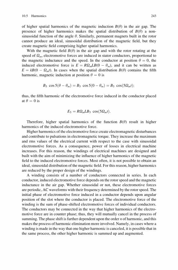
of higher spatial harmonics of the magnetic induction B(y) in the air gap. The
presence of higher harmonics makes the spatial distribution of B(y) a non-
sinusoidal function of the angle y. Similarly, permanent magnets built in the rotor
cannot produce an ideal, sinusoidal distribution of the magnetic field, but they
create magnetic field comprising higher spatial harmonics.
With the magnetic field B(y) in the air gap and with the rotor rotating at the
speed of Om, electromotive forces are induced in stator conductors, proportional to
the magnetic inductance and the speed. In the conductor at position y ¼ 0, the
induced electromotive force is E ¼ ROmLB(0 � ym), and it can be written as
E ¼ kB(0 � Omt). In cases when the spatial distribution B(y) contains the fifth
harmonic, magnetic induction at position y ¼ 0 is
B5 cos 5 y� ymð Þ ¼ B5 cos 5 0� ymð Þ ¼ B5 cos 5Omtð Þ;
thus, the fifth harmonic of the electromotive force induced in the conductor placed
at y ¼ 0 is
E5 ¼ ROmLB5 cos 5Omtð Þ:
Therefore, higher spatial harmonics of the function B(y) result in higher
harmonics of the induced electromotive force.
Higher harmonics of the electromotive force create electromagnetic disturbances
and contribute to pulsations in electromagnetic torque. They increase the maximum
and rms values of the electrical current with respect to the case with sinusoidal
electromotive forces. As a consequence, power of losses in electrical machine
increases. For this reason, the windings of electrical machines are designed and
built with the aim of minimizing the influence of higher harmonics of the magnetic
field to the induced electromotive forces. Most often, it is not possible to obtain an
ideal, sinusoidal distribution of the magnetic field. For this reason, higher harmonics
are reduced by the proper design of the windings.
A winding consists of a number of conductors connected in series. In each
conductor, induced electromotive force depends on the rotor speed and the magnetic
inductance in the air gap. Whether sinusoidal or not, these electromotive forces
are periodic, ACwaveforms with their frequency determined by the rotor speed. The
initial phase of electromotive force induced in a conductor depends upon angular
position of the slot where the conductor is placed. The electromotive force of the
winding is the sum of phase-shifted electromotive forces of individual conductors.
The conductors may be connected in the way that higher harmonics of the electro-
motive force are in counter phase; thus, they will mutually cancel in the process of
summing. The phase shift is further dependent upon the order n of harmonic, and this
makes the process of harmonic elimination more involved. Namely, in cases where a
winding is made in the way that one higher harmonic is canceled, it is possible that in
the same process, the other higher harmonic is summed up and augmented.
10.5 Harmonics 243
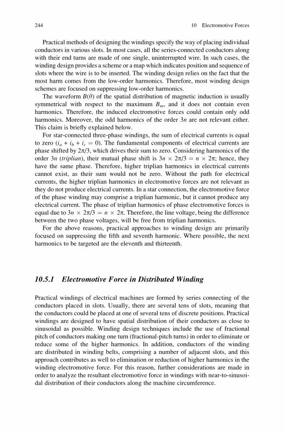
Practical methods of designing the windings specify the way of placing individual
conductors in various slots. In most cases, all the series-connected conductors along
with their end turns are made of one single, uninterrupted wire. In such cases, the
winding design provides a scheme or a map which indicates position and sequence of
slots where the wire is to be inserted. The winding design relies on the fact that the
most harm comes from the low-order harmonics. Therefore, most winding design
schemes are focused on suppressing low-order harmonics.
The waveform B(y) of the spatial distribution of magnetic induction is usually
symmetrical with respect to the maximum Bm, and it does not contain even
harmonics. Therefore, the induced electromotive forces could contain only odd
harmonics. Moreover, the odd harmonics of the order 3n are not relevant either.
This claim is briefly explained below.
For star-connected three-phase windings, the sum of electrical currents is equal
to zero (ia + ib + ic ¼ 0). The fundamental components of electrical currents are
phase shifted by 2p/3, which drives their sum to zero. Considering harmonics of the
order 3n (triplian), their mutual phase shift is 3n � 2p/3 ¼ n � 2p; hence, theyhave the same phase. Therefore, higher triplian harmonics in electrical currents
cannot exist, as their sum would not be zero. Without the path for electrical
currents, the higher triplian harmonics in electromotive forces are not relevant as
they do not produce electrical currents. In a star connection, the electromotive force
of the phase winding may comprise a triplian harmonic, but it cannot produce any
electrical current. The phase of triplian harmonics of phase electromotive forces is
equal due to 3n � 2p/3 ¼ n � 2p. Therefore, the line voltage, being the differencebetween the two phase voltages, will be free from triplian harmonics.
For the above reasons, practical approaches to winding design are primarily
focused on suppressing the fifth and seventh harmonic. Where possible, the next
harmonics to be targeted are the eleventh and thirteenth.
10.5.1 Electromotive Force in Distributed Winding
Practical windings of electrical machines are formed by series connecting of the
conductors placed in slots. Usually, there are several tens of slots, meaning that
the conductors could be placed at one of several tens of discrete positions. Practical
windings are designed to have spatial distribution of their conductors as close to
sinusoidal as possible. Winding design techniques include the use of fractional
pitch of conductors making one turn (fractional-pitch turns) in order to eliminate or
reduce some of the higher harmonics. In addition, conductors of the winding
are distributed in winding belts, comprising a number of adjacent slots, and this
approach contributes as well to elimination or reduction of higher harmonics in the
winding electromotive force. For this reason, further considerations are made in
order to analyze the resultant electromotive force in windings with near-to-sinusoi-
dal distribution of their conductors along the machine circumference.
244 10 Electromotive Forces
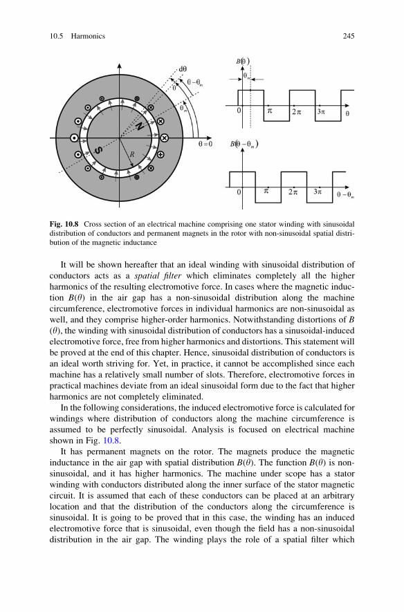
It will be shown hereafter that an ideal winding with sinusoidal distribution of
conductors acts as a spatial filter which eliminates completely all the higher
harmonics of the resulting electromotive force. In cases where the magnetic induc-
tion B(y) in the air gap has a non-sinusoidal distribution along the machine
circumference, electromotive forces in individual harmonics are non-sinusoidal as
well, and they comprise higher-order harmonics. Notwithstanding distortions of B(y), the winding with sinusoidal distribution of conductors has a sinusoidal-inducedelectromotive force, free from higher harmonics and distortions. This statement will
be proved at the end of this chapter. Hence, sinusoidal distribution of conductors is
an ideal worth striving for. Yet, in practice, it cannot be accomplished since each
machine has a relatively small number of slots. Therefore, electromotive forces in
practical machines deviate from an ideal sinusoidal form due to the fact that higher
harmonics are not completely eliminated.
In the following considerations, the induced electromotive force is calculated for
windings where distribution of conductors along the machine circumference is
assumed to be perfectly sinusoidal. Analysis is focused on electrical machine
shown in Fig. 10.8.
It has permanent magnets on the rotor. The magnets produce the magnetic
inductance in the air gap with spatial distribution B(y). The function B(y) is non-sinusoidal, and it has higher harmonics. The machine under scope has a stator
winding with conductors distributed along the inner surface of the stator magnetic
circuit. It is assumed that each of these conductors can be placed at an arbitrary
location and that the distribution of the conductors along the circumference is
sinusoidal. It is going to be proved that in this case, the winding has an induced
electromotive force that is sinusoidal, even though the field has a non-sinusoidal
distribution in the air gap. The winding plays the role of a spatial filter which
Fig. 10.8 Cross section of an electrical machine comprising one stator winding with sinusoidal
distribution of conductors and permanent magnets in the rotor with non-sinusoidal spatial distri-
bution of the magnetic inductance
10.5 Harmonics 245
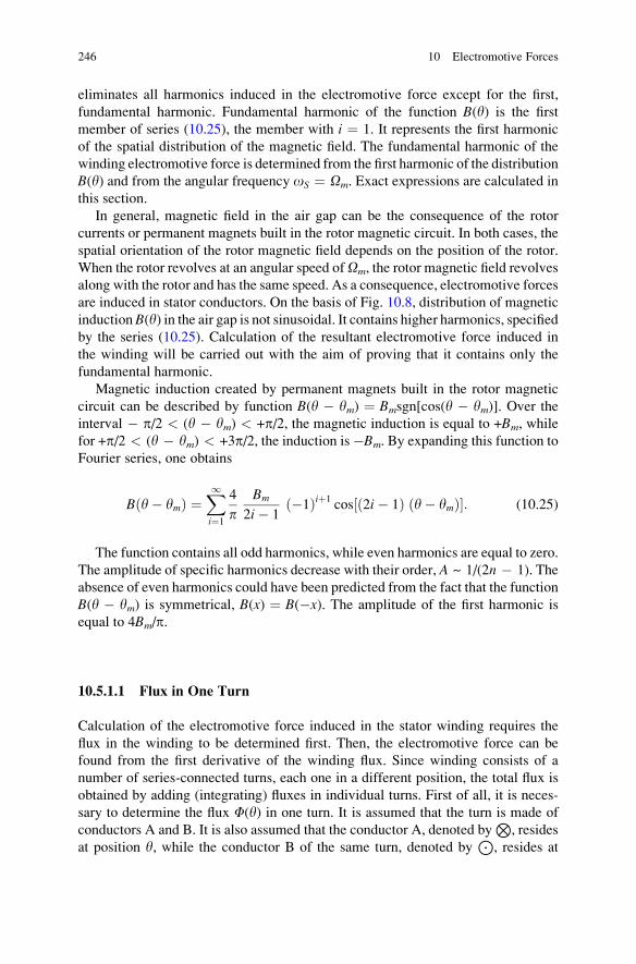
eliminates all harmonics induced in the electromotive force except for the first,
fundamental harmonic. Fundamental harmonic of the function B(y) is the first
member of series (10.25), the member with i ¼ 1. It represents the first harmonic
of the spatial distribution of the magnetic field. The fundamental harmonic of the
winding electromotive force is determined from the first harmonic of the distribution
B(y) and from the angular frequency oS ¼ Om. Exact expressions are calculated in
this section.
In general, magnetic field in the air gap can be the consequence of the rotor
currents or permanent magnets built in the rotor magnetic circuit. In both cases, the
spatial orientation of the rotor magnetic field depends on the position of the rotor.
When the rotor revolves at an angular speed ofOm, the rotor magnetic field revolves
along with the rotor and has the same speed. As a consequence, electromotive forces
are induced in stator conductors. On the basis of Fig. 10.8, distribution of magnetic
inductionB(y) in the air gap is not sinusoidal. It contains higher harmonics, specified
by the series (10.25). Calculation of the resultant electromotive force induced in
the winding will be carried out with the aim of proving that it contains only the
fundamental harmonic.
Magnetic induction created by permanent magnets built in the rotor magnetic
circuit can be described by function B(y � ym) ¼ Bmsgn[cos(y � ym)]. Over theinterval � p/2 < (y � ym) < +p/2, the magnetic induction is equal to +Bm, while
for +p/2 < (y � ym) < +3p/2, the induction is�Bm. By expanding this function to
Fourier series, one obtains
B y� ymð Þ ¼X1i¼1
4
pBm
2i� 1�1ð Þiþ1
cos 2i� 1ð Þ y� ymð Þ½ �: (10.25)
The function contains all odd harmonics, while even harmonics are equal to zero.
The amplitude of specific harmonics decrease with their order, A ~ 1/(2n � 1). The
absence of even harmonics could have been predicted from the fact that the function
B(y � ym) is symmetrical, B(x) ¼ B(�x). The amplitude of the first harmonic is
equal to 4Bm/p.
10.5.1.1 Flux in One Turn
Calculation of the electromotive force induced in the stator winding requires the
flux in the winding to be determined first. Then, the electromotive force can be
found from the first derivative of the winding flux. Since winding consists of a
number of series-connected turns, each one in a different position, the total flux is
obtained by adding (integrating) fluxes in individual turns. First of all, it is neces-
sary to determine the flux F(y) in one turn. It is assumed that the turn is made of
conductors A and B. It is also assumed that the conductor A, denoted byN
, resides
at position y, while the conductor B of the same turn, denoted byJ
, resides at
246 10 Electromotive Forces
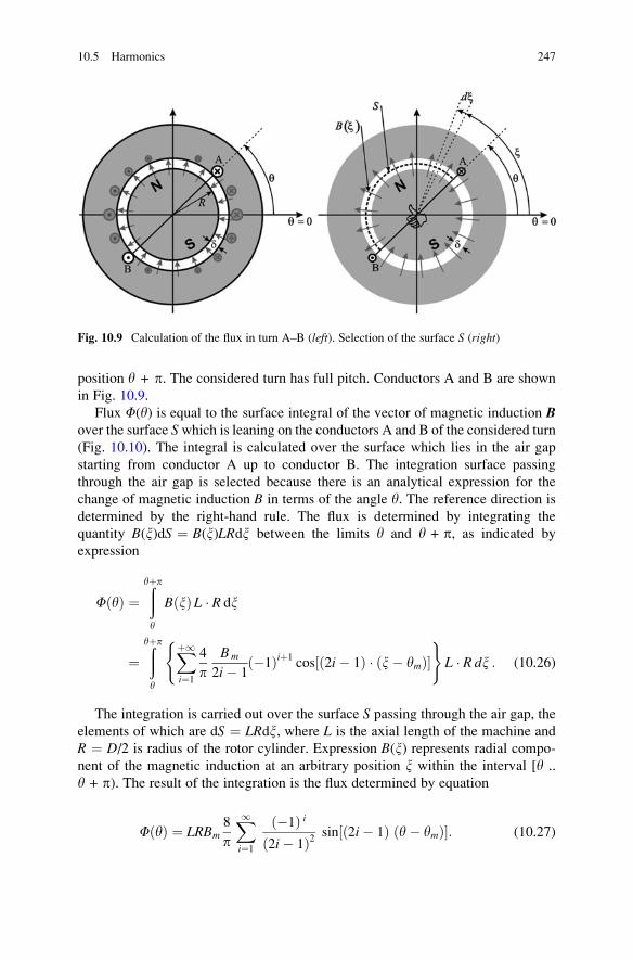
position y + p. The considered turn has full pitch. Conductors A and B are shown
in Fig. 10.9.
Flux F(y) is equal to the surface integral of the vector of magnetic induction Bover the surface Swhich is leaning on the conductors A and B of the considered turn
(Fig. 10.10). The integral is calculated over the surface which lies in the air gap
starting from conductor A up to conductor B. The integration surface passing
through the air gap is selected because there is an analytical expression for the
change of magnetic induction B in terms of the angle y. The reference direction is
determined by the right-hand rule. The flux is determined by integrating the
quantity B(x)dS ¼ B(x)LRdx between the limits y and y + p, as indicated by
expression
F yð Þ ¼ðyþp
y
B xð Þ L � R dx
¼ðyþp
y
Xþ1
i¼1
4
pBm
2i� 1�1ð Þiþ1
cos ð2i� 1Þ � ðx� ymÞ½ �( )
L � Rdx : (10.26)
The integration is carried out over the surface S passing through the air gap, the
elements of which are dS ¼ LRdx, where L is the axial length of the machine and
R ¼ D/2 is radius of the rotor cylinder. Expression B(x) represents radial compo-
nent of the magnetic induction at an arbitrary position x within the interval [y ..
y + p). The result of the integration is the flux determined by equation
F yð Þ ¼ LRBm8
p
X1i¼1
�1ð Þ i2i� 1ð Þ2 sin 2i� 1ð Þ y� ymð Þ½ �: (10.27)
Fig. 10.9 Calculation of the flux in turn A–B (left). Selection of the surface S (right)
10.5 Harmonics 247
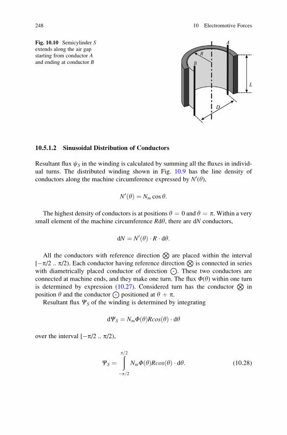
10.5.1.2 Sinusoidal Distribution of Conductors
Resultant flux cS in the winding is calculated by summing all the fluxes in individ-
ual turns. The distributed winding shown in Fig. 10.9 has the line density of
conductors along the machine circumference expressed by N0(y),
N0ðyÞ ¼ Nm cos y:
The highest density of conductors is at positions y ¼ 0 and y ¼ p. Within a very
small element of the machine circumference Rdy, there are dN conductors,
dN ¼ N0ðyÞ � R � dy:
All the conductors with reference directionN
are placed within the interval
[�p/2 .. p/2). Each conductor having reference directionN
is connected in series
with diametrically placed conductor of directionJ
. These two conductors are
connected at machine ends, and they make one turn. The flux F(y) within one turn
is determined by expression (10.27). Considered turn has the conductorN
in
position y and the conductorJ
positioned at y þ p.Resultant flux CS of the winding is determined by integrating
dCS ¼ NmF yð ÞRcos yð Þ � dy
over the interval [�p/2 .. p/2),
CS ¼ðp=2
�p=2
NmF yð ÞRcos yð Þ � dy: (10.28)
Fig. 10.10 Semicylinder Sextends along the air gap
starting from conductor Aand ending at conductor B
248 10 Electromotive Forces
By introducing F(y) from expression (10.27), one obtains that the flux of the
winding is
CS ¼ NmLR2Bm
8
p
X1i¼1
�1ð Þ i2i� 1ð Þ2
ðþp=2
�p=2
sin 2i� 1ð Þ y� ymð Þ½ � cos y � dy (10.29)
If the integrand of the integral (10.29) is written in the form
f y; ið Þ ¼ sin 2i� 1ð Þ y� ymð Þ½ � cos yð Þ¼ 1 2 sinð2iy� 2i� 1ð ÞymÞ þ sinð 2i� 2ð Þy� 2i� 1ð ÞymÞ½ �= ;
while the value of (NmLR2Bm�8/p) is denoted by k, the result (10.29) can be
represented as the sum in which each element is an integral of the function f(y,i)within limits �p/2 and p/2,
CS ¼ kX1i¼1
�1ð Þ i2i� 1ð Þ2
ðþp=2
�p=2
f y; ið Þ � dy:
For i � 2, each of the elements of the function f(y,i) is a sine function with an
integer number of its periods on the interval [�p/2 .. p/2). Therefore, the integral off(y,i) over the interval has a non zero value only for i ¼ 1. Any other of the sum but
the first is equal to zero. For the first member of the sum, for i ¼ 1, the integrand
becomes
f y; 1ð Þ ¼ sinð2y� ymÞ þ sinð�ymÞ½ �=2:
Introducing this expression in (10.29), for i ¼ 1, one obtains
C1S ¼ NmLR
2Bm8
p�1ð Þ 12� 1ð Þ2
ðþp=2
�p=2
sin y� ymð Þ cos yð Þ dy;
which gives the resultant flux in the winding. It has been demonstrated that only the
first (fundamental) harmonic of the non-sinusoidal distribution B(y) of the magnetic
induction produces the flux in the winding which has sinusoidal distribution of its
conductors. Since
ðþp=2
�p=2
sin y� ymð Þ cos yð Þ� dy ¼ 1
2
ðþp=2
�p=2
sin 2y� ymð Þ þ sin �ymð Þ½ � � dy
¼ � 1
4cos 2y� ymð Þ
����þp=2
�p=2þ 1
2sin �ymð Þ � y
����þp=2
�p=2¼ � p
2sin ym;
10.5 Harmonics 249
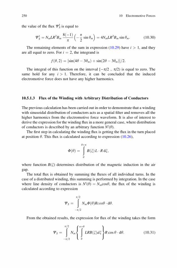
the value of the flux CS1 is equal to
C1S ¼ NmLR
2Bm8 �1ð Þp
� p2sin ym
� �¼ 4NmLR
2Bm sin ym: (10.30)
The remaining elements of the sum in expression (10.29) have i > 1, and they
are all equal to zero. For i ¼ 2, the integrand is
f y; 2ð Þ ¼ sinð4y� 3ymÞ þ sinð2y� 3ymÞ½ �=2:The integral of this function on the interval [�p/2 .. p/2) is equal to zero. The
same hold for any i > 1. Therefore, it can be concluded that the induced
electromotive force does not have any higher harmonics.
10.5.1.3 Flux of the Winding with Arbitrary Distribution of Conductors
The previous calculation has been carried out in order to demonstrate that a winding
with sinusoidal distribution of conductors acts as a spatial filter and removes all the
higher harmonics from the electromotive force waveform. It is also of interest to
derive the expression for the winding flux in a more general case, where distribution
of conductors is described by an arbitrary function N0(y).The first step in calculating the winding flux is getting the flux in the turn placed
at position y. This flux is calculated according to expression (10.26),
F yð Þ ¼ðyþp
y
B xð Þ L � R dx;
where function B(x) determines distribution of the magnetic induction in the air
gap.
The total flux is obtained by summing the fluxes of all individual turns. In the
case of a distributed winding, this summing is performed by integration. In the case
where line density of conductors is N0(y) ¼ Nmcosy, the flux of the winding is
calculated according to expression
CS ¼ðp=2
�p=2
NmF yð ÞRcosy � dy:
From the obtained results, the expression for flux of the winding takes the form
CS ¼ðp=2
�p=2
Nm
ðpþy
y
LRBðxÞdx8<:
9=;R cos y � dy: (10.31)
250 10 Electromotive Forces
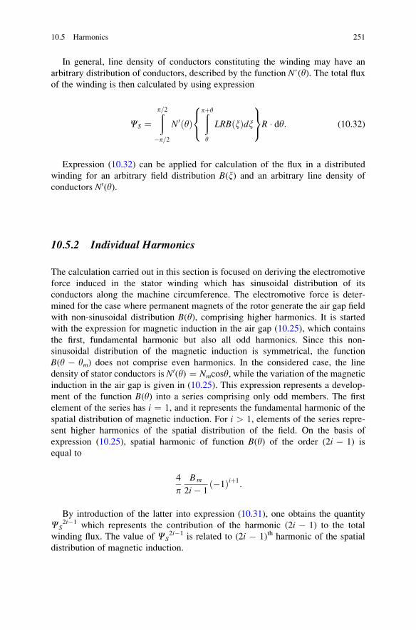
In general, line density of conductors constituting the winding may have an
arbitrary distribution of conductors, described by the function N’(y). The total fluxof the winding is then calculated by using expression
CS ¼ðp=2
�p=2
N0 yð Þðpþy
y
LRBðxÞdx8<:
9=;R � dy: (10.32)
Expression (10.32) can be applied for calculation of the flux in a distributed
winding for an arbitrary field distribution B(x) and an arbitrary line density of
conductors N0(y).
10.5.2 Individual Harmonics
The calculation carried out in this section is focused on deriving the electromotive
force induced in the stator winding which has sinusoidal distribution of its
conductors along the machine circumference. The electromotive force is deter-
mined for the case where permanent magnets of the rotor generate the air gap field
with non-sinusoidal distribution B(y), comprising higher harmonics. It is started
with the expression for magnetic induction in the air gap (10.25), which contains
the first, fundamental harmonic but also all odd harmonics. Since this non-
sinusoidal distribution of the magnetic induction is symmetrical, the function
B(y � ym) does not comprise even harmonics. In the considered case, the line
density of stator conductors is N0(y) ¼ Nmcosy, while the variation of the magnetic
induction in the air gap is given in (10.25). This expression represents a develop-
ment of the function B(y) into a series comprising only odd members. The first
element of the series has i ¼ 1, and it represents the fundamental harmonic of the
spatial distribution of magnetic induction. For i > 1, elements of the series repre-
sent higher harmonics of the spatial distribution of the field. On the basis of
expression (10.25), spatial harmonic of function B(y) of the order (2i � 1) is
equal to
4
pBm
2i� 1�1ð Þiþ1:
By introduction of the latter into expression (10.31), one obtains the quantity
CS2i�1 which represents the contribution of the harmonic (2i � 1) to the total
winding flux. The value of CS2i�1 is related to (2i � 1)th harmonic of the spatial
distribution of magnetic induction.
10.5 Harmonics 251
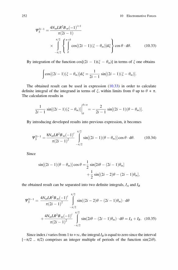
C2i�1S ¼ 4NmLR
2Bm �1ð Þiþ1
p 2i� 1ð Þ
�ðp=2
�p=2
ðpþy
y
cos 2i� 1ð Þ x� ymð Þ½ �dx8<:
9=; cos y � dy: (10.33)
By integration of the function cos[(2i � 1)(x � ym)] in terms of x one obtains
ðcos 2i� 1ð Þ x� ymð Þ½ �dx ¼ 1
2i� 1sin 2i� 1ð Þ x� ymð Þ½ �:
The obtained result can be used in expression (10.33) in order to calculate
definite integral of the integrand in terms of x, within limits from y up to y + p.The calculation results in
1
2i� 1sin 2i� 1ð Þ x� ymð Þ½ �
����yþp
y¼ � 2
2i� 1sin 2i� 1ð Þ y� ymð Þ½ �:
By introducing developed results into previous expression, it becomes
C2i�1S ¼ 8NmLR
2Bm �1ð Þip 2i� 1ð Þ2
ðp=2
�p=2
sin 2i� 1ð Þ y� ymð Þ½ � cos y � dy: (10.34)
Since
sin 2i� 1ð Þ y� ymð Þ½ � cos y ¼ 1
2sin 2iy� 2i� 1ð Þym½ �
þ 1
2sin 2i� 2ð Þy� 2i� 1ð Þym½ �;
the obtained result can be separated into two definite integrals, IA and IB
C2i�1S ¼ 4NmLR
2Bm �1ð Þip 2i� 1ð Þ2
ðp=2
�p=2
sin 2i� 2ð Þy� 2i� 1ð Þymð Þ � dy
þ 4NmLR2Bm �1ð Þi
p 2i� 1ð Þ2ðp=2
�p=2
sin 2iy� 2i� 1ð Þymð Þ � dy ¼ IA þ IB: (10.35)
Since index i varies from 1 to +1, the integral IB is equal to zero since the interval[�p/2 .. p/2) comprises an integer multiple of periods of the function sin(2iy).
252 10 Electromotive Forces
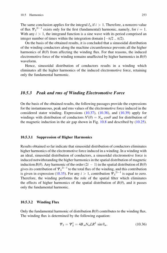
The same conclusion applies for the integral IA if i > 1. Therefore, a nonzero value
of flux CS2i�1 exists only for the first (fundamental) harmonic, namely, for i ¼ 1.
With any i > 1, the integrand function is a sine wave with its period comprised an
integer number of times within the integration domain [�p/2 .. p/2).On the basis of the obtained results, it is concluded that a sinusoidal distribution
of the winding conductors along the machine circumference prevents all the higher
harmonics of B(y) from affecting the winding flux. For that reasons, the induced
electromotive force of the winding remains unaffected by higher harmonics in B(y)waveform.
Hence, sinusoidal distribution of conductors results in a winding which
eliminates all the higher harmonics of the induced electromotive force, retaining
only the fundamental harmonic.
10.5.3 Peak and rms of Winding Electromotive Force
On the basis of the obtained results, the following passages provide the expressions
for the instantaneous, peak and rms values of the electromotive force induced in the
considered stator winding. Expressions (10.37), (10.38), and (10.39) apply for
windings with distribution of conductors N0(y) ¼ Nm cosy and for distribution of
the magnetic induction in the air gap shown in Fig. 10.8 and described by (10.25).
10.5.3.1 Suppression of Higher Harmonics
Results obtained so far indicate that sinusoidal distribution of conductors eliminates
higher harmonics of the electromotive force induced in a winding. In a winding with
an ideal, sinusoidal distribution of conductors, a sinusoidal electromotive force is
induced notwithstanding the higher harmonics in the spatial distribution of magnetic
induction B(y). Any harmonic of the order (2i � 1) in the spatial distribution of B(y)gives its contribution ofCS
2i�1 to the total flux of the winding, and this contribution
is given in expression (10.35). For any i > 1, contribution CS2i�1 is equal to zero.
Therefore, the winding performs the role of the spatial filter which eliminates
the effects of higher harmonics of the spatial distribution of B(y), and it passes
only the fundamental harmonic.
10.5.3.2 Winding Flux
Only the fundamental harmonic of distribution B(y) contributes to the winding flux.The winding flux is determined by the following equation:
CS ¼ C1S ¼ 4BmNmLR
2 sin ym: (10.36)
10.5 Harmonics 253
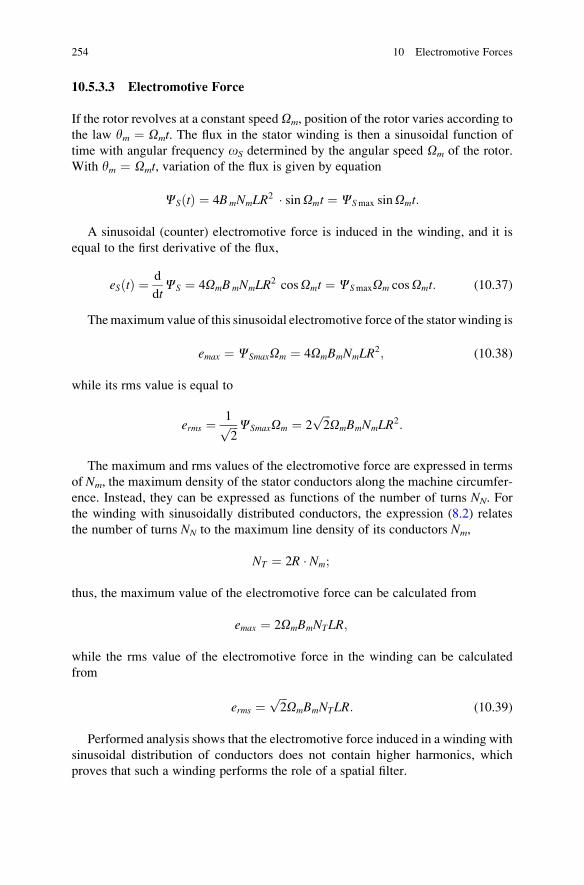
10.5.3.3 Electromotive Force
If the rotor revolves at a constant speed Om, position of the rotor varies according to
the law ym ¼ Omt. The flux in the stator winding is then a sinusoidal function of
time with angular frequency oS determined by the angular speed Om of the rotor.
With ym ¼ Omt, variation of the flux is given by equation
CSðtÞ ¼ 4BmNmLR2 � sinOmt ¼ CSmax sinOmt:
A sinusoidal (counter) electromotive force is induced in the winding, and it is
equal to the first derivative of the flux,
eSðtÞ ¼ d
dtCS ¼ 4OmBmNmLR
2 cosOmt ¼ CSmaxOm cosOmt: (10.37)
Themaximum value of this sinusoidal electromotive force of the stator winding is
emax ¼ CSmaxOm ¼ 4OmBmNmLR2; (10.38)
while its rms value is equal to
erms ¼ 1ffiffiffi2
p CSmaxOm ¼ 2ffiffiffi2
pOmBmNmLR
2:
The maximum and rms values of the electromotive force are expressed in terms
of Nm, the maximum density of the stator conductors along the machine circumfer-
ence. Instead, they can be expressed as functions of the number of turns NN. For
the winding with sinusoidally distributed conductors, the expression (8.2) relates
the number of turns NN to the maximum line density of its conductors Nm,
NT ¼ 2R � Nm;
thus, the maximum value of the electromotive force can be calculated from
emax ¼ 2OmBmNTLR;
while the rms value of the electromotive force in the winding can be calculated
from
erms ¼ffiffiffi2
pOmBmNTLR: (10.39)
Performed analysis shows that the electromotive force induced in a winding with
sinusoidal distribution of conductors does not contain higher harmonics, which
proves that such a winding performs the role of a spatial filter.
254 10 Electromotive Forces
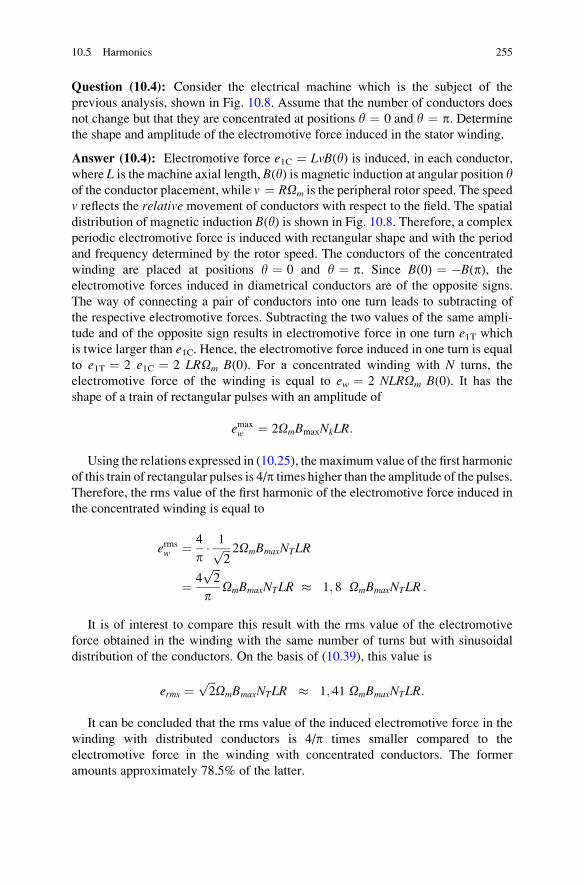
Question (10.4): Consider the electrical machine which is the subject of the
previous analysis, shown in Fig. 10.8. Assume that the number of conductors does
not change but that they are concentrated at positions y ¼ 0 and y ¼ p. Determine
the shape and amplitude of the electromotive force induced in the stator winding.
Answer (10.4): Electromotive force e1C ¼ LvB(y) is induced, in each conductor,
where L is the machine axial length, B(y) is magnetic induction at angular position yof the conductor placement, while v ¼ ROm is the peripheral rotor speed. The speed
v reflects the relative movement of conductors with respect to the field. The spatial
distribution of magnetic induction B(y) is shown in Fig. 10.8. Therefore, a complex
periodic electromotive force is induced with rectangular shape and with the period
and frequency determined by the rotor speed. The conductors of the concentrated
winding are placed at positions y ¼ 0 and y ¼ p. Since B(0) ¼ �B(p), the
electromotive forces induced in diametrical conductors are of the opposite signs.
The way of connecting a pair of conductors into one turn leads to subtracting of
the respective electromotive forces. Subtracting the two values of the same ampli-
tude and of the opposite sign results in electromotive force in one turn e1T which
is twice larger than e1C. Hence, the electromotive force induced in one turn is equal
to e1T ¼ 2 e1C ¼ 2 LROm B(0). For a concentrated winding with N turns, the
electromotive force of the winding is equal to ew ¼ 2 NLROm B(0). It has the
shape of a train of rectangular pulses with an amplitude of
emaxw ¼ 2OmBmaxNkLR:
Using the relations expressed in (10.25), the maximum value of the first harmonic
of this train of rectangular pulses is 4/p times higher than the amplitude of the pulses.
Therefore, the rms value of the first harmonic of the electromotive force induced in
the concentrated winding is equal to
ermsw ¼ 4
p� 1ffiffiffi
2p 2OmBmaxNTLR
¼ 4ffiffiffi2
p
pOmBmaxNTLR � 1; 8 OmBmaxNTLR :
It is of interest to compare this result with the rms value of the electromotive
force obtained in the winding with the same number of turns but with sinusoidal
distribution of the conductors. On the basis of (10.39), this value is
erms ¼ffiffiffi2
pOmBmaxNTLR � 1; 41 OmBmaxNTLR:
It can be concluded that the rms value of the induced electromotive force in the
winding with distributed conductors is 4/p times smaller compared to the
electromotive force in the winding with concentrated conductors. The former
amounts approximately 78.5% of the latter.
10.5 Harmonics 255
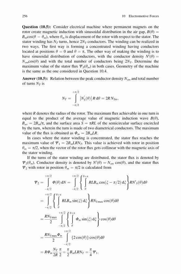
Question (10.5): Consider electrical machine where permanent magnets on the
rotor create magnetic induction with sinusoidal distribution in the air gap, B(y) ¼Bmcos(y � ym), where ym is displacement of the rotor with respect to the stator. The
stator winding has NT turns, hence 2NT conductors. The winding can be realized in
two ways. The first way is forming a concentrated winding having conductors
located at positions y ¼ 0 and y ¼ p. The other way of making the winding is to
have sinusoidal distribution of conductors, with the conductor density N0(y) ¼Nsmcos(y) and with the total number of conductors being 2NT. Determine the
maximum value of the stator flux CS(ym) in both cases. Geometry of the machine
is the same as the one considered in Question 10.4.
Answer (10.5): Relation between the peak conductor density Nsm and total number
of turns NT is
NT ¼ðþp=2
�p=2
N0S yð Þ�� ��R dy ¼ 2RNSm;
where R denotes the radius of the rotor. The maximum flux achievable in one turn is
equal to the product of the average value of magnetic induction wave B(y),Bav ¼ 2Bm/p, and the surface area S ¼ pRL of the semicircular surface encircled
by the turn, wherein the turn is made of two diametrical conductors. The maximum
value of the flux is obtained as Fm ¼ 2BmLR.In cases where the stator winding is concentrated, the stator flux reaches the
maximum value of C1 ¼ 2BmLRNT. This value is achieved with rotor in position
ym ¼ p/2, when the vector of the rotor flux gets collinear with the magnetic axis of
the stator winding.
If the turns of the stator winding are distributed, the stator flux is denoted by
C2(ym). Conductor density is denoted by N0(y) ¼ Nsm cos(y), and the stator flux
C2 with rotor in position ym ¼ p/2 is calculated from
C2 ¼ðþp=2
�p=2
F yð Þ dN ¼ðþp=2
�p=2
ðyþp
y
RLBm cos x� p=2ð Þ dx8<:
9=;RN0
S yð Þdy
¼ðþp=2
�p=2
ðyþp
y
RLBm sin xð Þ dx8<:
9=;RNSmax cos yð Þdy
¼ RNSmax
2
ðþp=2
�p=2
ðyþp
y
Fm sin xð Þ dx8<:
9=; cos yð Þdy
¼ RNSmaxFm
2
ðþp=2
�p=2
2 cos yð Þf g cos yð Þdy
¼ RFmNT
2R
p2¼ p
2BmLRNT ¼ p
4C1:
256 10 Electromotive Forces
Based on the above calculation, conclusion is drawn that, all the remaining
conditions being equal, the machine with sinusoidally distributed stator winding has
the peak stator flux which is p/4 times lower than the peak stator flux in the machine
with concentrated stator winding.
10.5 Harmonics 257
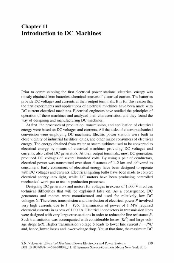
Chapter 11
Introduction to DC Machines
Prior to commissioning the first electrical power stations, electrical energy was
mostly obtained from batteries, chemical sources of electrical current. The batteries
provide DC voltages and currents at their output terminals. It is for this reason that
the first experiments and applications of electrical machines have been made with
DC current electrical machines. Electrical engineers have studied the principles of
operation of these machines and analyzed their characteristics, and they found the
way of designing and manufacturing DC machines.
At first, the processes of production, transmission, and application of electrical
energy were based on DC voltages and currents. All the tasks of electromechanical
conversion were employing DC machines. Electric power stations were built in
close vicinity of industrial facilities, cities, and other major consumers of electrical
energy. The energy obtained from water or steam turbines used to be converted to
electrical energy by means of electrical machines providing DC voltages and
currents, also called DC generators. At their output terminals, most DC generators
produced DC voltages of several hundred volts. By using a pair of conductors,
electrical power was transmitted over short distances of 1–2 km and delivered to
consumers. Early consumers of electrical energy have been designed to operate
with DC voltages and currents. Electrical lighting bulbs have been made to convert
electrical energy into light, while DC motors have been producing controlled
mechanical work put to use in production processes.
Designing DC generators and motors for voltages in excess of 1,000 V involves
technical difficulties that will be explained later on. As a consequence, DC
generators and motors were manufactured and used for relatively low DC
voltages U. Therefore, transmission and distribution of electrical power P involved
very high currents due to I ¼ P/U. Transmission of power of 1 MW required
electrical currents in excess of 1,000 A. Electrical conductors in transmission lines
were designed with very large cross sections in order to reduce the line resistance R.Such transmission was accompanied with considerable losses (RI2) and large volt-
age drops (RI). Higher transmission voltage U leads to lower line current I ¼ P/Uand, hence, lower losses and lower voltage drop. Yet, at that time, the maximumDC
S.N. Vukosavic, Electrical Machines, Power Electronics and Power Systems,
DOI 10.1007/978-1-4614-0400-2_11, # Springer Science+Business Media New York 2013
259
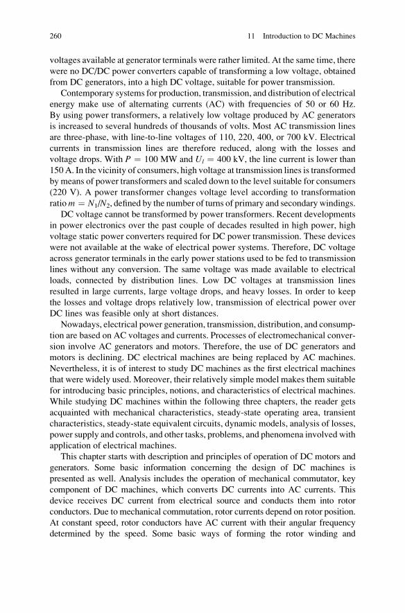
voltages available at generator terminals were rather limited. At the same time, there
were no DC/DC power converters capable of transforming a low voltage, obtained
from DC generators, into a high DC voltage, suitable for power transmission.
Contemporary systems for production, transmission, and distribution of electrical
energy make use of alternating currents (AC) with frequencies of 50 or 60 Hz.
By using power transformers, a relatively low voltage produced by AC generators
is increased to several hundreds of thousands of volts. Most AC transmission lines
are three-phase, with line-to-line voltages of 110, 220, 400, or 700 kV. Electrical
currents in transmission lines are therefore reduced, along with the losses and
voltage drops. With P ¼ 100 MW and Ul ¼ 400 kV, the line current is lower than
150 A. In the vicinity of consumers, high voltage at transmission lines is transformed
by means of power transformers and scaled down to the level suitable for consumers
(220 V). A power transformer changes voltage level according to transformation
ratiom ¼ N1/N2, defined by the number of turns of primary and secondary windings.
DC voltage cannot be transformed by power transformers. Recent developments
in power electronics over the past couple of decades resulted in high power, high
voltage static power converters required for DC power transmission. These devices
were not available at the wake of electrical power systems. Therefore, DC voltage
across generator terminals in the early power stations used to be fed to transmission
lines without any conversion. The same voltage was made available to electrical
loads, connected by distribution lines. Low DC voltages at transmission lines
resulted in large currents, large voltage drops, and heavy losses. In order to keep
the losses and voltage drops relatively low, transmission of electrical power over
DC lines was feasible only at short distances.
Nowadays, electrical power generation, transmission, distribution, and consump-
tion are based on AC voltages and currents. Processes of electromechanical conver-
sion involve AC generators and motors. Therefore, the use of DC generators and
motors is declining. DC electrical machines are being replaced by AC machines.
Nevertheless, it is of interest to study DC machines as the first electrical machines
that were widely used. Moreover, their relatively simple model makes them suitable
for introducing basic principles, notions, and characteristics of electrical machines.
While studying DC machines within the following three chapters, the reader gets
acquainted with mechanical characteristics, steady-state operating area, transient
characteristics, steady-state equivalent circuits, dynamic models, analysis of losses,
power supply and controls, and other tasks, problems, and phenomena involved with
application of electrical machines.
This chapter starts with description and principles of operation of DC motors and
generators. Some basic information concerning the design of DC machines is
presented as well. Analysis includes the operation of mechanical commutator, key
component of DC machines, which converts DC currents into AC currents. This
device receives DC current from electrical source and conducts them into rotor
conductors. Due to mechanical commutation, rotor currents depend on rotor position.
At constant speed, rotor conductors have AC current with their angular frequency
determined by the speed. Some basic ways of forming the rotor winding and
260 11 Introduction to DC Machines
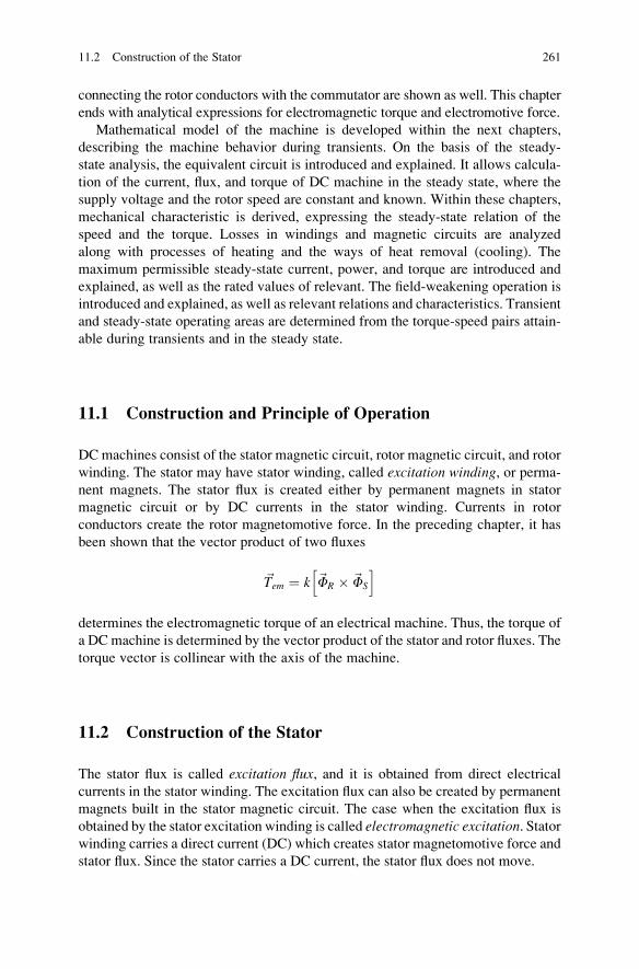
connecting the rotor conductors with the commutator are shown as well. This chapter
ends with analytical expressions for electromagnetic torque and electromotive force.
Mathematical model of the machine is developed within the next chapters,
describing the machine behavior during transients. On the basis of the steady-
state analysis, the equivalent circuit is introduced and explained. It allows calcula-
tion of the current, flux, and torque of DC machine in the steady state, where the
supply voltage and the rotor speed are constant and known. Within these chapters,
mechanical characteristic is derived, expressing the steady-state relation of the
speed and the torque. Losses in windings and magnetic circuits are analyzed
along with processes of heating and the ways of heat removal (cooling). The
maximum permissible steady-state current, power, and torque are introduced and
explained, as well as the rated values of relevant. The field-weakening operation is
introduced and explained, as well as relevant relations and characteristics. Transient
and steady-state operating areas are determined from the torque-speed pairs attain-
able during transients and in the steady state.
11.1 Construction and Principle of Operation
DCmachines consist of the stator magnetic circuit, rotor magnetic circuit, and rotor
winding. The stator may have stator winding, called excitation winding, or perma-
nent magnets. The stator flux is created either by permanent magnets in stator
magnetic circuit or by DC currents in the stator winding. Currents in rotor
conductors create the rotor magnetomotive force. In the preceding chapter, it has
been shown that the vector product of two fluxes
~Tem ¼ k ~FR � ~FS
h i
determines the electromagnetic torque of an electrical machine. Thus, the torque of
a DC machine is determined by the vector product of the stator and rotor fluxes. The
torque vector is collinear with the axis of the machine.
11.2 Construction of the Stator
The stator flux is called excitation flux, and it is obtained from direct electrical
currents in the stator winding. The excitation flux can also be created by permanent
magnets built in the stator magnetic circuit. The case when the excitation flux is
obtained by the stator excitation winding is called electromagnetic excitation. Statorwinding carries a direct current (DC) which creates stator magnetomotive force and
stator flux. Since the stator carries a DC current, the stator flux does not move.
11.2 Construction of the Stator 261
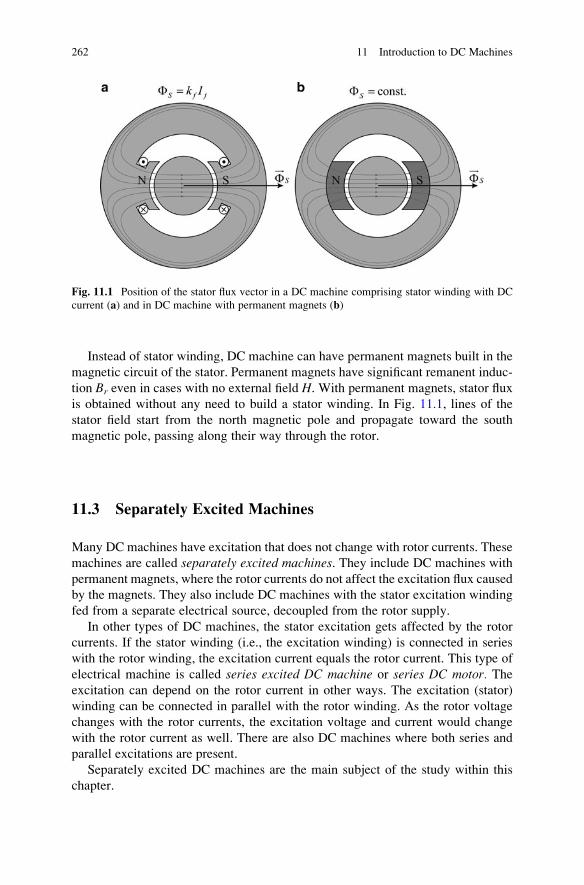
Instead of stator winding, DC machine can have permanent magnets built in the
magnetic circuit of the stator. Permanent magnets have significant remanent induc-
tion Br even in cases with no external field H. With permanent magnets, stator flux
is obtained without any need to build a stator winding. In Fig. 11.1, lines of the
stator field start from the north magnetic pole and propagate toward the south
magnetic pole, passing along their way through the rotor.
11.3 Separately Excited Machines
Many DC machines have excitation that does not change with rotor currents. These
machines are called separately excited machines. They include DC machines with
permanent magnets, where the rotor currents do not affect the excitation flux caused
by the magnets. They also include DC machines with the stator excitation winding
fed from a separate electrical source, decoupled from the rotor supply.
In other types of DC machines, the stator excitation gets affected by the rotor
currents. If the stator winding (i.e., the excitation winding) is connected in series
with the rotor winding, the excitation current equals the rotor current. This type of
electrical machine is called series excited DC machine or series DC motor. Theexcitation can depend on the rotor current in other ways. The excitation (stator)
winding can be connected in parallel with the rotor winding. As the rotor voltage
changes with the rotor currents, the excitation voltage and current would change
with the rotor current as well. There are also DC machines where both series and
parallel excitations are present.
Separately excited DC machines are the main subject of the study within this
chapter.
Fig. 11.1 Position of the stator flux vector in a DC machine comprising stator winding with DC
current (a) and in DC machine with permanent magnets (b)
262 11 Introduction to DC Machines
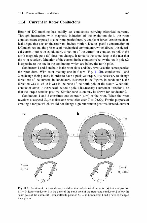
11.4 Current in Rotor Conductors
Rotor of DC machine has axially set conductors carrying electrical currents.
Through interaction with magnetic induction of the excitation field, the rotor
conductors are exposed to electromagnetic force. A couple of forces create mechan-
ical torque that acts on the rotor and incites motion. Due to specific construction of
DCmachines and the presence of mechanical commutator, which directs the electri-
cal current into rotor conductors, direction of the current in conductors below the
north magnetic pole (N) does not change. It remains the same despite the fact that
the rotor revolves. Direction of the current in the conductors below the south pole (S)is opposite to the one in the conductors which are below the north pole.
Conductors 1 and 2 are built in the rotor slots, and they revolve at the same speed as
the rotor does. With rotor making one half turn (Fig. 11.2b), conductors 1 and
2 exchange their places. In order to have a positive torque, it is necessary to change
directions of the currents in conductors, as shown in the Figure. In conductor 1, the
direction was � while it was in the zone of the north pole of the stator. When this
conductor comes to the zone of the south pole, it has to carry a current of direction� so
that the torque remains positive. Similar conclusion may be drawn for conductor 2.
Conductors 1 and 2 constitute one contour (turn) of the rotor. When the rotor
revolves at a speedOm, it makes one revolution each T ¼ 2p/Om. For the purpose of
creating a torque which would not change sign but remain positive instead, current
Fig. 11.2 Position of rotor conductors and directions of electrical currents. (a) Rotor at position
ym ¼ 0. Rotor conductor 1 in the zone of the north pole of the stator and conductor 2 below the
south pole of the stator. (b) Rotor shifted to position ym ¼ p. Conductors 1 and 2 have exchangedtheir places
11.4 Current in Rotor Conductors 263
through the considered contour should change sign synchronously with the rotor
movement. The current should be positive during time interval T/2 ¼ p/Om and
then negative during the next interval of T/2. Therefore, current in the rotor has to
be periodic with the period T determined by the rotor speed.
The ways of directing the rotor currents into conductors so as to obtain periodic
electrical currents will be put aside at this time. By considering Fig. 11.2 and
assuming that, notwithstanding the rotor motion, electrical current in rotor conduc-
tor below the north pole retains direction �, while the conductor below the south
pole always has direction of the current �, the rotor magnetomotive force and flux
can be represented by vectors directed downward. On the other hand, vector of the
stator field is horizontal, directed from left to right. It is concluded that the angle
between the two fluxes is constant and equal to p/2, irrespective of the speed and
direction of the rotor motion. This fulfills the optimal condition for creating
constant torque.
Considered pair of rotor conductors is in the region under the stator poles. Coupled
forces producing positive torque act upon conductors 1 and 2 (Fig. 11.2a). This torque
supports counterclockwise movement. The electromagnetic torque is determined by
(11.1) where l is length of one conductor, B is magnetic induction in the zones of the
stator magnetic poles, and D is rotor diameter.
~F ¼ ið~l� ~BÞ;
Mem ¼ l � B � i � D: (11.1)
11.5 Mechanical Commutator
Rotor currents in a DC machine are obtained from DC power sources. The source
current is fed to a mechanical commutator. The rotating part of the commutator is
called collector, while the stator part of the commutator has two carbon brushes
usually designated by A and B. External power supply that feeds the rotor winding
has its positive pole connected to the brush A and its negative pole to the brush B.
Attached to the stator, the brushes do not move. The collector is fastened to the rotor
shaft and rotates at the same speed as the rotor. Owing to this, the still carbon
brushes, positioned diametrically, slide along collector ring. A collector ring is
divided into a number of mutually insulated segments. The collector segments are
called commutator segments or collector segments. The segments have electrical
connection to rotor turns in the manner to be described later.
DC current from an external DC source is fed to diametrically positioned
brushes A and B. Immobile brushes lean on the collector segments, directing in
this way current into the rotor conductors. When the rotor moves, the brushes slide
from one pair of the collector segments to the next pair. As a consequence, a change
264 11 Introduction to DC Machines
occurs in distribution of electrical current in rotor conductors. The end result is
that, notwithstanding the rotor motion, the rotor currents create the magnetomotive
force vector FR12 which does not move with respect to the stator, as shown in
Fig. 11.2. The rotor magnetomotive force gives a rise to the rotor flux, which does
not move either.
Mechanical commutator converts DC currents, obtained from the power supply
of the rotor winding, to periodic currents carried by rotor conductors. Frequency of
these currents is determined by the speed of rotation. The role of the mechanical
commutator is similar to that of static power converters called inverters, which
employ power transistor switches and convert DC voltages and currents into AC
voltages and currents. The change of voltages and currents in conductors of the rotor
equipped with mechanical commutator is similar to the change of voltages and
currents in a system comprising DC supplied inverter which feeds AC currents
and supplies asynchronous or synchronous machines.
In modern applications of electrical machines, DC machines with mechanical
commutator are replaced by static power converters (transistor inverters) feeding
asynchronous or synchronous machines, also called AC machines.
The method of making of rotor winding as well as the method of connecting this
winding to collector may be relatively involved. A detailed study of different
methods of realization of rotor windings of DC machines is beyond the scope of
this book. For the purpose of understanding the operation of mechanical commuta-
tor, further discussion presents an analysis of some relatively simple examples,
intended for illustration of basic functions of mechanical collector.
11.6 Rotor Winding
Figure 11.3 shows a rotor having only one turn. It is made of conductors 1 and 2
connected in series. The conductors are in electrical connection with collector which
has segments S1 and S2. Such collector can bemade from ametal cylinder by cutting
it in two mutually insulated halves. The front end of conductor 1 is connected to
segment S1, while the front end of conductor 2 is connected to segment S2. At the
rear end of the rotor, the ends of conductors 1 and 2 are brought together by the end
turn. Brushes A and B are connected to a current source supplying electrical current
i(t). In the given position, brushes A and B lean on segments S1 and S2, respectively.
Therefore, there is electrical contact between the brush and the segment that gets in
touch with it. At position presented in the figure, current in conductor 1 has direction
�, while current in conductor 2 has direction �. When the rotor moves by p,conductors exchange their places. At the same time, the segments S1 and S2 change
their places as well, as they are fastened to the rotor and revolve along with the rotor.
Now conductor 1 gets under the south pole (left), but direction of the electrical
current in this conductor is changed. Therefore, the electrical current in rotor con-
ductor under the north pole retains direction �, while the current in rotor conductor
under the south pole retains direction �. Mechanical commutator insures that the
11.6 Rotor Winding 265
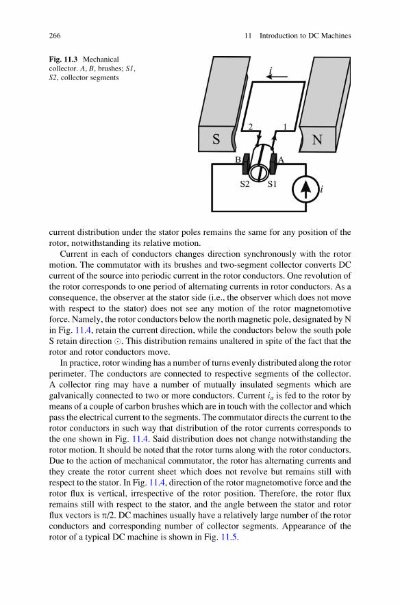
current distribution under the stator poles remains the same for any position of the
rotor, notwithstanding its relative motion.
Current in each of conductors changes direction synchronously with the rotor
motion. The commutator with its brushes and two-segment collector converts DC
current of the source into periodic current in the rotor conductors. One revolution of
the rotor corresponds to one period of alternating currents in rotor conductors. As a
consequence, the observer at the stator side (i.e., the observer which does not move
with respect to the stator) does not see any motion of the rotor magnetomotive
force. Namely, the rotor conductors below the north magnetic pole, designated by N
in Fig. 11.4, retain the current direction, while the conductors below the south pole
S retain direction �. This distribution remains unaltered in spite of the fact that the
rotor and rotor conductors move.
In practice, rotor winding has a number of turns evenly distributed along the rotor
perimeter. The conductors are connected to respective segments of the collector.
A collector ring may have a number of mutually insulated segments which are
galvanically connected to two or more conductors. Current ia is fed to the rotor by
means of a couple of carbon brushes which are in touch with the collector and which
pass the electrical current to the segments. The commutator directs the current to the
rotor conductors in such way that distribution of the rotor currents corresponds to
the one shown in Fig. 11.4. Said distribution does not change notwithstanding the
rotor motion. It should be noted that the rotor turns along with the rotor conductors.
Due to the action of mechanical commutator, the rotor has alternating currents and
they create the rotor current sheet which does not revolve but remains still with
respect to the stator. In Fig. 11.4, direction of the rotor magnetomotive force and the
rotor flux is vertical, irrespective of the rotor position. Therefore, the rotor flux
remains still with respect to the stator, and the angle between the stator and rotor
flux vectors is p/2. DC machines usually have a relatively large number of the rotor
conductors and corresponding number of collector segments. Appearance of the
rotor of a typical DC machine is shown in Fig. 11.5.
Fig. 11.3 Mechanical
collector. A, B, brushes; S1,S2, collector segments
266 11 Introduction to DC Machines
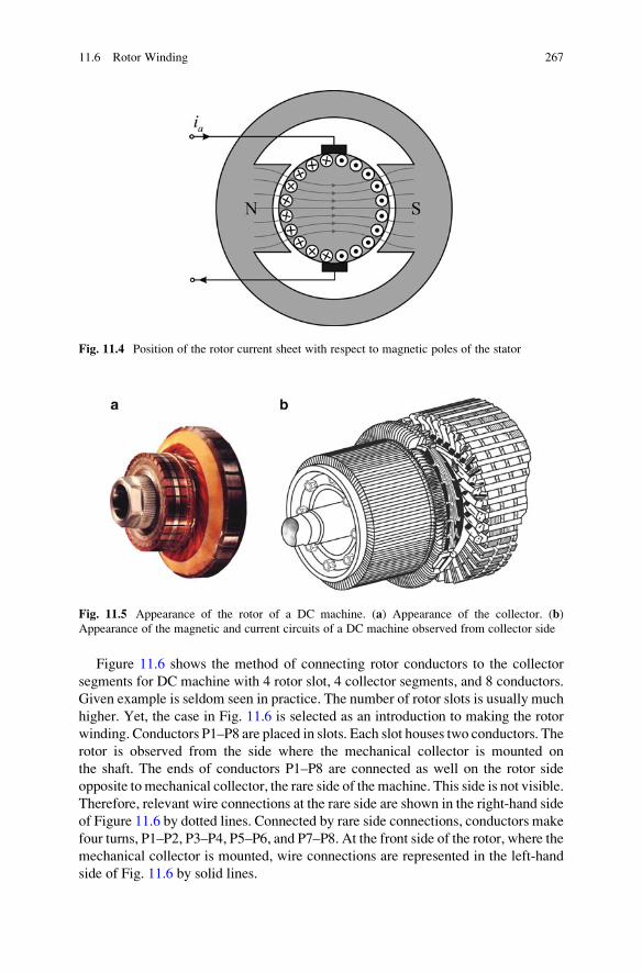
Figure 11.6 shows the method of connecting rotor conductors to the collector
segments for DC machine with 4 rotor slot, 4 collector segments, and 8 conductors.
Given example is seldom seen in practice. The number of rotor slots is usually much
higher. Yet, the case in Fig. 11.6 is selected as an introduction to making the rotor
winding. Conductors P1–P8 are placed in slots. Each slot houses two conductors. The
rotor is observed from the side where the mechanical collector is mounted on
the shaft. The ends of conductors P1–P8 are connected as well on the rotor side
opposite to mechanical collector, the rare side of the machine. This side is not visible.
Therefore, relevant wire connections at the rare side are shown in the right-hand side
of Figure 11.6 by dotted lines. Connected by rare side connections, conductors make
four turns, P1–P2, P3–P4, P5–P6, and P7–P8. At the front side of the rotor, where the
mechanical collector is mounted, wire connections are represented in the left-hand
side of Fig. 11.6 by solid lines.
Fig. 11.4 Position of the rotor current sheet with respect to magnetic poles of the stator
Fig. 11.5 Appearance of the rotor of a DC machine. (a) Appearance of the collector. (b)
Appearance of the magnetic and current circuits of a DC machine observed from collector side
11.6 Rotor Winding 267
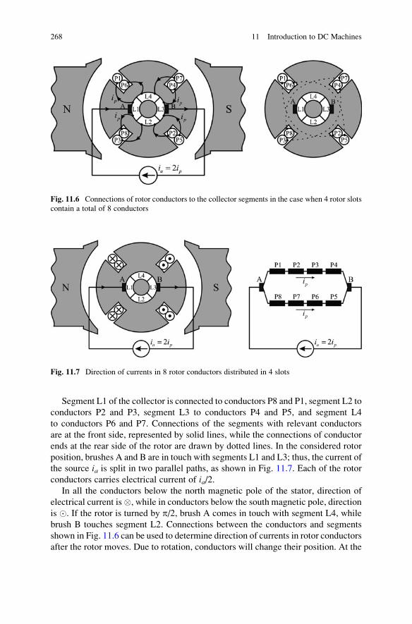
Segment L1 of the collector is connected to conductors P8 and P1, segment L2 to
conductors P2 and P3, segment L3 to conductors P4 and P5, and segment L4
to conductors P6 and P7. Connections of the segments with relevant conductors
are at the front side, represented by solid lines, while the connections of conductor
ends at the rear side of the rotor are drawn by dotted lines. In the considered rotor
position, brushes A and B are in touch with segments L1 and L3; thus, the current of
the source ia is split in two parallel paths, as shown in Fig. 11.7. Each of the rotor
conductors carries electrical current of ia/2.In all the conductors below the north magnetic pole of the stator, direction of
electrical current is�, while in conductors below the south magnetic pole, direction
is �. If the rotor is turned by p/2, brush A comes in touch with segment L4, while
brush B touches segment L2. Connections between the conductors and segments
shown in Fig. 11.6 can be used to determine direction of currents in rotor conductors
after the rotor moves. Due to rotation, conductors will change their position. At the
Fig. 11.6 Connections of rotor conductors to the collector segments in the case when 4 rotor slots
contain a total of 8 conductors
Fig. 11.7 Direction of currents in 8 rotor conductors distributed in 4 slots
268 11 Introduction to DC Machines
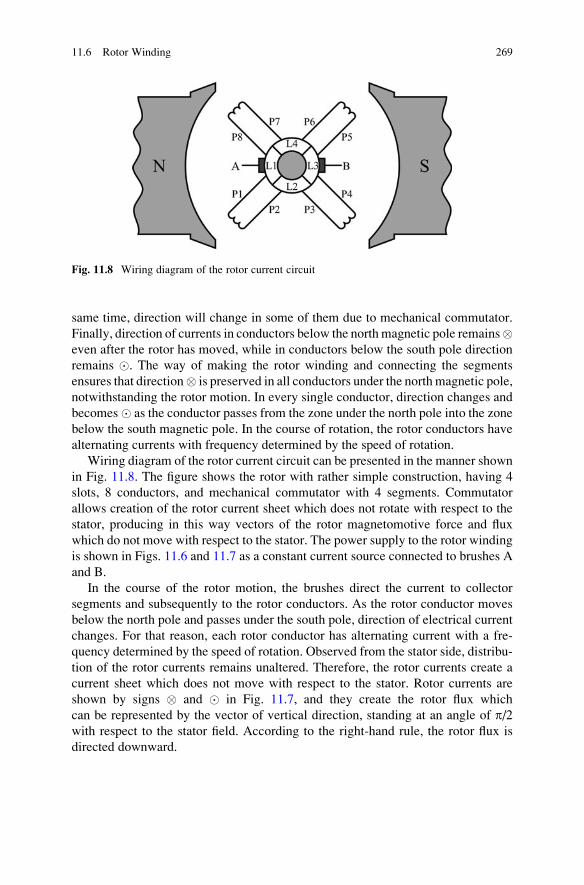
same time, direction will change in some of them due to mechanical commutator.
Finally, direction of currents in conductors below the north magnetic pole remains�even after the rotor has moved, while in conductors below the south pole direction
remains �. The way of making the rotor winding and connecting the segments
ensures that direction� is preserved in all conductors under the north magnetic pole,
notwithstanding the rotor motion. In every single conductor, direction changes and
becomes� as the conductor passes from the zone under the north pole into the zone
below the south magnetic pole. In the course of rotation, the rotor conductors have
alternating currents with frequency determined by the speed of rotation.
Wiring diagram of the rotor current circuit can be presented in the manner shown
in Fig. 11.8. The figure shows the rotor with rather simple construction, having 4
slots, 8 conductors, and mechanical commutator with 4 segments. Commutator
allows creation of the rotor current sheet which does not rotate with respect to the
stator, producing in this way vectors of the rotor magnetomotive force and flux
which do not move with respect to the stator. The power supply to the rotor winding
is shown in Figs. 11.6 and 11.7 as a constant current source connected to brushes A
and B.
In the course of the rotor motion, the brushes direct the current to collector
segments and subsequently to the rotor conductors. As the rotor conductor moves
below the north pole and passes under the south pole, direction of electrical current
changes. For that reason, each rotor conductor has alternating current with a fre-
quency determined by the speed of rotation. Observed from the stator side, distribu-
tion of the rotor currents remains unaltered. Therefore, the rotor currents create a
current sheet which does not move with respect to the stator. Rotor currents are
shown by signs � and � in Fig. 11.7, and they create the rotor flux which
can be represented by the vector of vertical direction, standing at an angle of p/2with respect to the stator field. According to the right-hand rule, the rotor flux is
directed downward.
Fig. 11.8 Wiring diagram of the rotor current circuit
11.6 Rotor Winding 269
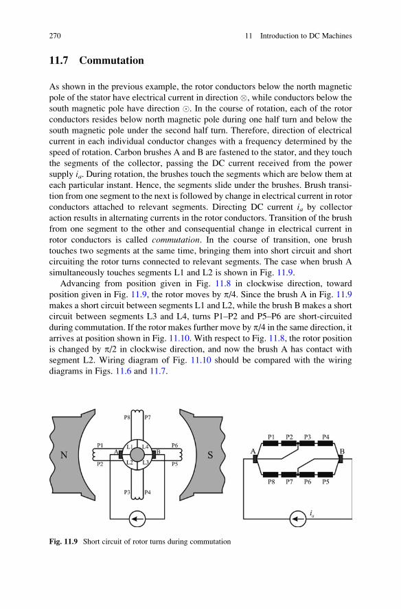
11.7 Commutation
As shown in the previous example, the rotor conductors below the north magnetic
pole of the stator have electrical current in direction �, while conductors below the
south magnetic pole have direction �. In the course of rotation, each of the rotor
conductors resides below north magnetic pole during one half turn and below the
south magnetic pole under the second half turn. Therefore, direction of electrical
current in each individual conductor changes with a frequency determined by the
speed of rotation. Carbon brushes A and B are fastened to the stator, and they touch
the segments of the collector, passing the DC current received from the power
supply ia. During rotation, the brushes touch the segments which are below them at
each particular instant. Hence, the segments slide under the brushes. Brush transi-
tion from one segment to the next is followed by change in electrical current in rotor
conductors attached to relevant segments. Directing DC current ia by collector
action results in alternating currents in the rotor conductors. Transition of the brush
from one segment to the other and consequential change in electrical current in
rotor conductors is called commutation. In the course of transition, one brush
touches two segments at the same time, bringing them into short circuit and short
circuiting the rotor turns connected to relevant segments. The case when brush A
simultaneously touches segments L1 and L2 is shown in Fig. 11.9.
Advancing from position given in Fig. 11.8 in clockwise direction, toward
position given in Fig. 11.9, the rotor moves by p/4. Since the brush A in Fig. 11.9
makes a short circuit between segments L1 and L2, while the brush B makes a short
circuit between segments L3 and L4, turns P1–P2 and P5–P6 are short-circuited
during commutation. If the rotor makes further move by p/4 in the same direction, it
arrives at position shown in Fig. 11.10. With respect to Fig. 11.8, the rotor position
is changed by p/2 in clockwise direction, and now the brush A has contact with
segment L2. Wiring diagram of Fig. 11.10 should be compared with the wiring
diagrams in Figs. 11.6 and 11.7.
Fig. 11.9 Short circuit of rotor turns during commutation
270 11 Introduction to DC Machines
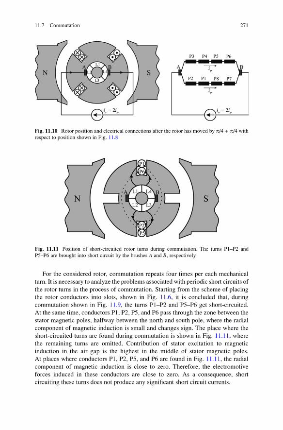
For the considered rotor, commutation repeats four times per each mechanical
turn. It is necessary to analyze the problems associated with periodic short circuits of
the rotor turns in the process of commutation. Starting from the scheme of placing
the rotor conductors into slots, shown in Fig. 11.6, it is concluded that, during
commutation shown in Fig. 11.9, the turns P1–P2 and P5–P6 get short-circuited.
At the same time, conductors P1, P2, P5, and P6 pass through the zone between the
stator magnetic poles, halfway between the north and south pole, where the radial
component of magnetic induction is small and changes sign. The place where the
short-circuited turns are found during commutation is shown in Fig. 11.11, where
the remaining turns are omitted. Contribution of stator excitation to magnetic
induction in the air gap is the highest in the middle of stator magnetic poles.
At places where conductors P1, P2, P5, and P6 are found in Fig. 11.11, the radial
component of magnetic induction is close to zero. Therefore, the electromotive
forces induced in these conductors are close to zero. As a consequence, short
circuiting these turns does not produce any significant short circuit currents.
Fig. 11.10 Rotor position and electrical connections after the rotor has moved by p/4 + p/4 with
respect to position shown in Fig. 11.8
Fig. 11.11 Position of short-circuited rotor turns during commutation. The turns P1–P2 and
P5–P6 are brought into short circuit by the brushes A and B, respectively
11.7 Commutation 271
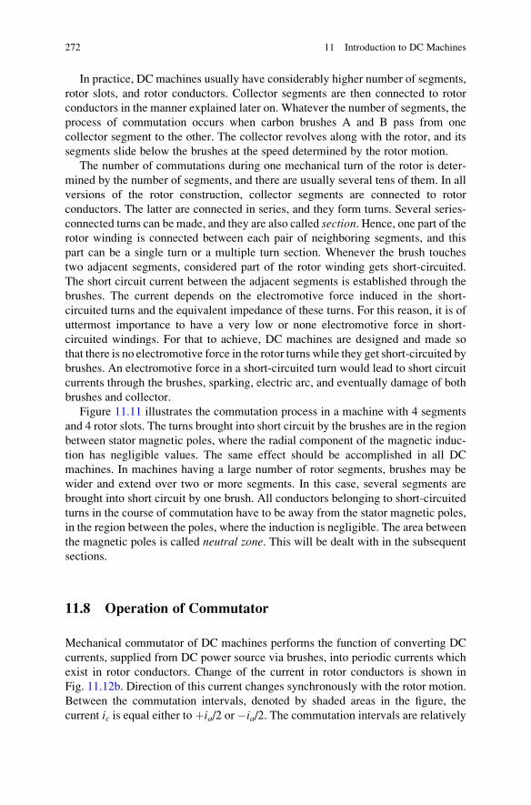
In practice, DC machines usually have considerably higher number of segments,
rotor slots, and rotor conductors. Collector segments are then connected to rotor
conductors in the manner explained later on. Whatever the number of segments, the
process of commutation occurs when carbon brushes A and B pass from one
collector segment to the other. The collector revolves along with the rotor, and its
segments slide below the brushes at the speed determined by the rotor motion.
The number of commutations during one mechanical turn of the rotor is deter-
mined by the number of segments, and there are usually several tens of them. In all
versions of the rotor construction, collector segments are connected to rotor
conductors. The latter are connected in series, and they form turns. Several series-
connected turns can be made, and they are also called section. Hence, one part of therotor winding is connected between each pair of neighboring segments, and this
part can be a single turn or a multiple turn section. Whenever the brush touches
two adjacent segments, considered part of the rotor winding gets short-circuited.
The short circuit current between the adjacent segments is established through the
brushes. The current depends on the electromotive force induced in the short-
circuited turns and the equivalent impedance of these turns. For this reason, it is of
uttermost importance to have a very low or none electromotive force in short-
circuited windings. For that to achieve, DC machines are designed and made so
that there is no electromotive force in the rotor turns while they get short-circuited by
brushes. An electromotive force in a short-circuited turn would lead to short circuit
currents through the brushes, sparking, electric arc, and eventually damage of both
brushes and collector.
Figure 11.11 illustrates the commutation process in a machine with 4 segments
and 4 rotor slots. The turns brought into short circuit by the brushes are in the region
between stator magnetic poles, where the radial component of the magnetic induc-
tion has negligible values. The same effect should be accomplished in all DC
machines. In machines having a large number of rotor segments, brushes may be
wider and extend over two or more segments. In this case, several segments are
brought into short circuit by one brush. All conductors belonging to short-circuited
turns in the course of commutation have to be away from the stator magnetic poles,
in the region between the poles, where the induction is negligible. The area between
the magnetic poles is called neutral zone. This will be dealt with in the subsequent
sections.
11.8 Operation of Commutator
Mechanical commutator of DC machines performs the function of converting DC
currents, supplied from DC power source via brushes, into periodic currents which
exist in rotor conductors. Change of the current in rotor conductors is shown in
Fig. 11.12b. Direction of this current changes synchronously with the rotor motion.
Between the commutation intervals, denoted by shaded areas in the figure, the
current ic is equal either to þia/2 or �ia/2. The commutation intervals are relatively
272 11 Introduction to DC Machines
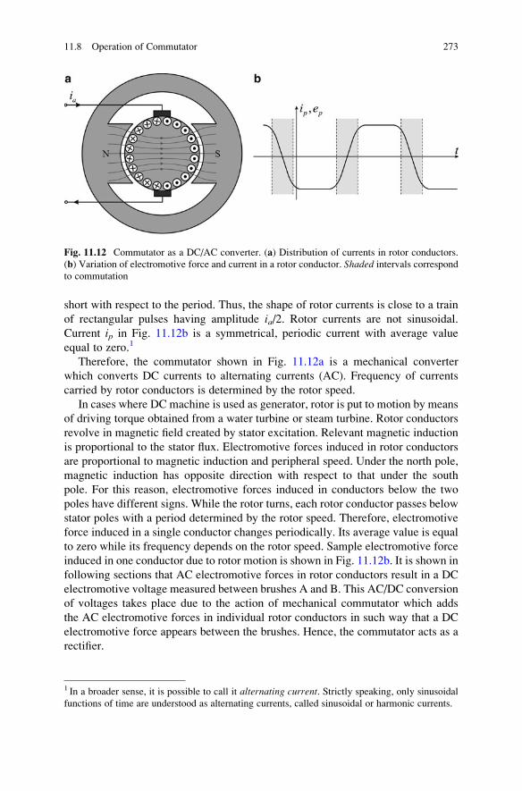
short with respect to the period. Thus, the shape of rotor currents is close to a train
of rectangular pulses having amplitude ia/2. Rotor currents are not sinusoidal.
Current ip in Fig. 11.12b is a symmetrical, periodic current with average value
equal to zero.1
Therefore, the commutator shown in Fig. 11.12a is a mechanical converter
which converts DC currents to alternating currents (AC). Frequency of currents
carried by rotor conductors is determined by the rotor speed.
In cases where DC machine is used as generator, rotor is put to motion by means
of driving torque obtained from a water turbine or steam turbine. Rotor conductors
revolve in magnetic field created by stator excitation. Relevant magnetic induction
is proportional to the stator flux. Electromotive forces induced in rotor conductors
are proportional to magnetic induction and peripheral speed. Under the north pole,
magnetic induction has opposite direction with respect to that under the south
pole. For this reason, electromotive forces induced in conductors below the two
poles have different signs. While the rotor turns, each rotor conductor passes below
stator poles with a period determined by the rotor speed. Therefore, electromotive
force induced in a single conductor changes periodically. Its average value is equal
to zero while its frequency depends on the rotor speed. Sample electromotive force
induced in one conductor due to rotor motion is shown in Fig. 11.12b. It is shown in
following sections that AC electromotive forces in rotor conductors result in a DC
electromotive voltage measured between brushes A and B. This AC/DC conversion
of voltages takes place due to the action of mechanical commutator which adds
the AC electromotive forces in individual rotor conductors in such way that a DC
electromotive force appears between the brushes. Hence, the commutator acts as a
rectifier.
Fig. 11.12 Commutator as a DC/AC converter. (a) Distribution of currents in rotor conductors.
(b) Variation of electromotive force and current in a rotor conductor. Shaded intervals correspondto commutation
1 In a broader sense, it is possible to call it alternating current. Strictly speaking, only sinusoidal
functions of time are understood as alternating currents, called sinusoidal or harmonic currents.
11.8 Operation of Commutator 273
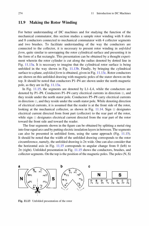
11.9 Making the Rotor Winding
For better understanding of DC machines and for studying the function of the
mechanical commutator, this section studies a sample rotor winding with 8 slots
and 8 conductors connected to mechanical commutator with 4 collector segments
and two brushes. To facilitate understanding of the way the conductors are
connected to the collector, it is necessary to present rotor winding in unfoldedform, quite similar to unwrapping the rotor cylindrical surface and presenting it in
the form of a flat rectangle. This presentation can be obtained by a thought experi-
ment wherein the rotor cylinder is cut along the radius denoted by dotted line in
Fig. 11.13a. It is necessary to imagine that the cylindrical rotor surface is being
unfolded in the way shown in Fig. 11.13b. Finally, by bringing the cylindrical
surface to a plane, unfolded form is obtained, given in Fig. 11.13c. Rotor conductors
are shown on this unfolded drawing with magnetic poles of the stator shown on the
top. It should be noted that conductors P1–P4 are shown under the north magnetic
pole, as they are in Fig. 11.13a.
In Fig. 11.15, the segments are denoted by L1–L4, while the conductors are
denoted by P1–P8. Conductors P1–P4 carry electrical currents in direction �, and
they reside under the north stator pole. Conductors P5–P8 carry electrical currents
in direction�, and they reside under the south stator pole. While denoting direction
of electrical currents, it is assumed that the reader is at the front side of the rotor,
looking at the mechanical collector, as shown in Fig. 11.14. Sign � designates
electrical current directed from front part (collector) to the rear part of the rotor,
while sign � designates electrical current directed from the rear part of the rotor
toward the front side and toward the reader.
The four segments shown in the figure can be obtained by splitting a metal ring
into four equal arcs and by putting electric insulation layers in between. The segments
can also be presented in unfolded form, using the same approach (Fig. 11.15).
It should be noted that the width of the unfolded drawing corresponds to the rotor
circumference, namely, the unfolded drawing is 2p wide. One can also consider that
the horizontal axis in Fig. 11.15 corresponds to angular change from 0 (left) to
2p (right). Unfolded presentation in Fig. 11.15 shows the conductors, brushes, and
collector segments. On the top is the position of the magnetic poles. The poles (N, S)
Fig. 11.13 Unfolded presentation of the rotor
274 11 Introduction to DC Machines
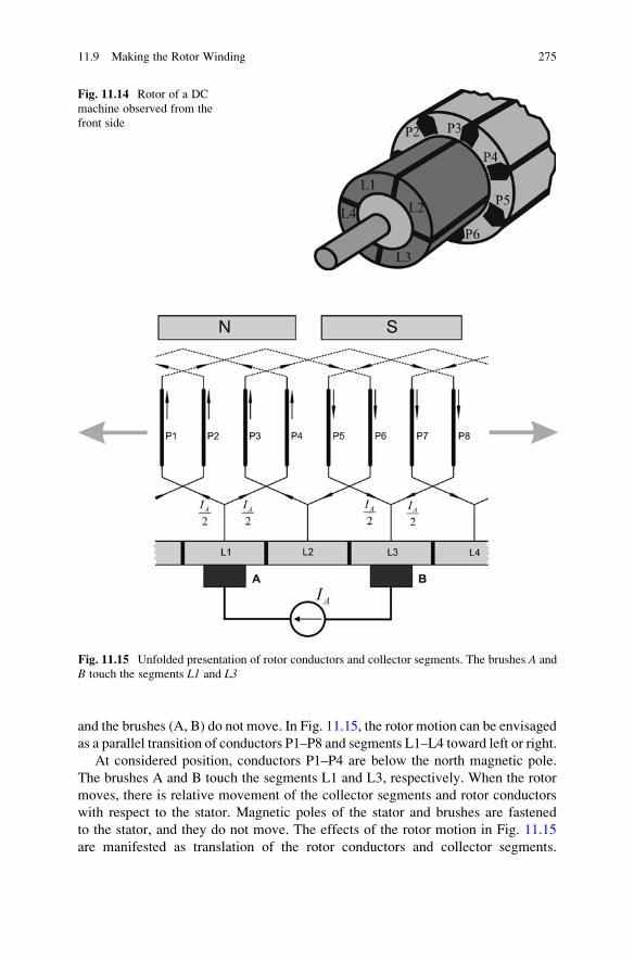
and the brushes (A, B) do not move. In Fig. 11.15, the rotor motion can be envisaged
as a parallel transition of conductors P1–P8 and segments L1–L4 toward left or right.
At considered position, conductors P1–P4 are below the north magnetic pole.
The brushes A and B touch the segments L1 and L3, respectively. When the rotor
moves, there is relative movement of the collector segments and rotor conductors
with respect to the stator. Magnetic poles of the stator and brushes are fastened
to the stator, and they do not move. The effects of the rotor motion in Fig. 11.15
are manifested as translation of the rotor conductors and collector segments.
Fig. 11.15 Unfolded presentation of rotor conductors and collector segments. The brushes A and
B touch the segments L1 and L3
Fig. 11.14 Rotor of a DC
machine observed from the
front side
11.9 Making the Rotor Winding 275
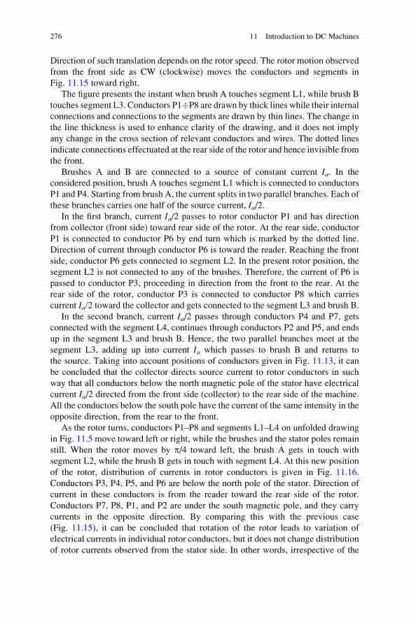
Direction of such translation depends on the rotor speed. The rotor motion observed
from the front side as CW (clockwise) moves the conductors and segments in
Fig. 11.15 toward right.
The figure presents the instant when brush A touches segment L1, while brush B
touches segment L3. Conductors P1�P8 are drawn by thick lines while their internal
connections and connections to the segments are drawn by thin lines. The change in
the line thickness is used to enhance clarity of the drawing, and it does not imply
any change in the cross section of relevant conductors and wires. The dotted lines
indicate connections effectuated at the rear side of the rotor and hence invisible from
the front.
Brushes A and B are connected to a source of constant current Ia. In the
considered position, brush A touches segment L1 which is connected to conductors
P1 and P4. Starting from brush A, the current splits in two parallel branches. Each of
these branches carries one half of the source current, Ia/2.In the first branch, current Ia/2 passes to rotor conductor P1 and has direction
from collector (front side) toward rear side of the rotor. At the rear side, conductor
P1 is connected to conductor P6 by end turn which is marked by the dotted line.
Direction of current through conductor P6 is toward the reader. Reaching the front
side, conductor P6 gets connected to segment L2. In the present rotor position, the
segment L2 is not connected to any of the brushes. Therefore, the current of P6 is
passed to conductor P3, proceeding in direction from the front to the rear. At the
rear side of the rotor, conductor P3 is connected to conductor P8 which carries
current Ia/2 toward the collector and gets connected to the segment L3 and brush B.
In the second branch, current Ia/2 passes through conductors P4 and P7, gets
connected with the segment L4, continues through conductors P2 and P5, and ends
up in the segment L3 and brush B. Hence, the two parallel branches meet at the
segment L3, adding up into current Ia which passes to brush B and returns to
the source. Taking into account positions of conductors given in Fig. 11.13, it can
be concluded that the collector directs source current to rotor conductors in such
way that all conductors below the north magnetic pole of the stator have electrical
current Ia/2 directed from the front side (collector) to the rear side of the machine.
All the conductors below the south pole have the current of the same intensity in the
opposite direction, from the rear to the front.
As the rotor turns, conductors P1–P8 and segments L1–L4 on unfolded drawing
in Fig. 11.5 move toward left or right, while the brushes and the stator poles remain
still. When the rotor moves by p/4 toward left, the brush A gets in touch with
segment L2, while the brush B gets in touch with segment L4. At this new position
of the rotor, distribution of currents in rotor conductors is given in Fig. 11.16.
Conductors P3, P4, P5, and P6 are below the north pole of the stator. Direction of
current in these conductors is from the reader toward the rear side of the rotor.
Conductors P7, P8, P1, and P2 are under the south magnetic pole, and they carry
currents in the opposite direction. By comparing this with the previous case
(Fig. 11.15), it can be concluded that rotation of the rotor leads to variation of
electrical currents in individual rotor conductors, but it does not change distribution
of rotor currents observed from the stator side. In other words, irrespective of the
276 11 Introduction to DC Machines
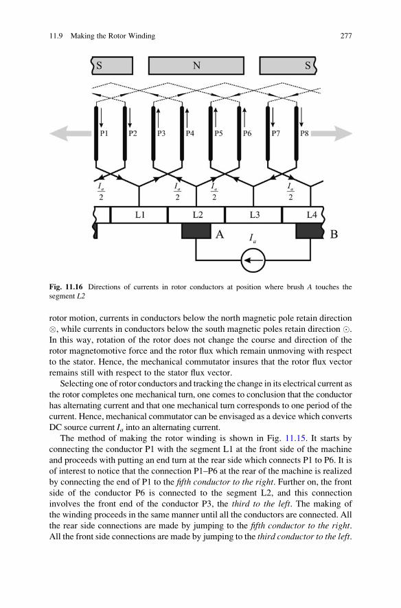
rotor motion, currents in conductors below the north magnetic pole retain direction
�, while currents in conductors below the south magnetic poles retain direction �.
In this way, rotation of the rotor does not change the course and direction of the
rotor magnetomotive force and the rotor flux which remain unmoving with respect
to the stator. Hence, the mechanical commutator insures that the rotor flux vector
remains still with respect to the stator flux vector.
Selecting one of rotor conductors and tracking the change in its electrical current as
the rotor completes one mechanical turn, one comes to conclusion that the conductor
has alternating current and that one mechanical turn corresponds to one period of the
current. Hence, mechanical commutator can be envisaged as a device which converts
DC source current Ia into an alternating current.The method of making the rotor winding is shown in Fig. 11.15. It starts by
connecting the conductor P1 with the segment L1 at the front side of the machine
and proceeds with putting an end turn at the rear side which connects P1 to P6. It is
of interest to notice that the connection P1–P6 at the rear of the machine is realized
by connecting the end of P1 to the fifth conductor to the right. Further on, the frontside of the conductor P6 is connected to the segment L2, and this connection
involves the front end of the conductor P3, the third to the left. The making of
the winding proceeds in the same manner until all the conductors are connected. All
the rear side connections are made by jumping to the fifth conductor to the right.All the front side connections are made by jumping to the third conductor to the left.
Fig. 11.16 Directions of currents in rotor conductors at position where brush A touches the
segment L2
11.9 Making the Rotor Winding 277
Besides, all the front side connections between the two conductors involve as well
connection to one collector segment. It should be noted that the turns made in the
prescribed way are fractional pitch turns. Full pitch turn would involve jumping to
the fourth conductor (i.e., slot), whether to left or right.
Explained is the basic principle of making the rotor winding. In practice, there
are a number of schemes being used. Most DC machines have more than eight slots.
The approach can be generalized. With rotor having 2N slots, connections at the
rear side are made with conductor in (N þ 1)-th slot to the right, while connections
at the collector side are made with conductor in (N � 1)-th slot to the left.
One slot usually accommodates several conductors. Therefore, the process of
making the rotor winding and connecting the winding to collector segments is more
complicated than the one illustrated in Fig. 11.15. Instead of placing only one turn
in two slots, it is possible to prepare a sectionmade of several turns and placing the
two sides of this section in two slots. It is also possible to place two groups of
conductors, each belonging to different sections, into the same slot. In such cases,
the winding is said to have two layers. The way of connecting the rotor conductors
shown in Fig. 11.15 results in a lap winding. There are also other ways, such as
wave windings.2
Figure 11.17 shows the front view of the rotor which is also given in Fig. 11.15
in its unfolded form. Signs � and � are associated with the rotor conductors. Full
lines marked by arrows show connections of rotor conductors at the front side.
Dotted lines show the connections between rotor conductors at the rear side of the
machine. Designation P1P6 next to the dotted line marks that this is connection
between conductors P1 and P6 made at the rear side of the rotor. A comparison of
this presentation with the one in Fig. 11.15 illustrates the merits of the unfolded
scheme.
11.10 Problems with Commutation
By considering the example of a rotor winding having 8 conductors and 4 collector
segments analyzed in the preceding section, it is concluded that at each instant,
there are two parallel branches between brushes A and B. In each of them, there are
4 conductors connected in series. Current in the rotor conductors is equal to one half
of the current taken from the source which is connected to the collector brushes and
which feeds the rotor winding.
When brush A passes from segment L1 to segment L2, brush B passes from
segment L3 to segment L4. Passage of brushes from one segment to another leads to
changes of direction of electrical currents in individual rotor conductors. In the
course of commutation, shown in Fig. 11.18, brush A makes a short circuit between
2More details on windings of electrical machines can be found in publication Pyrhonen J, Jokinen T,
Hrabovcova V (2008) Design of rotating electrical machines. Wiley, ISBN: 978-0-470-69516-6
278 11 Introduction to DC Machines
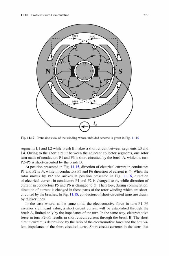
segments L1 and L2 while brush B makes a short circuit between segments L3 and
L4. Owing to the short circuit between the adjacent collector segments, one rotor
turn made of conductors P1 and P6 is short-circuited by the brush A, while the turn
P2–P5 is short-circuited by the brush B.
At position presented in Fig. 11.15, direction of electrical current in conductors
P1 and P2 is �, while in conductors P5 and P6 direction of current is �. When the
rotor moves by p/2 and arrives at position presented in Fig. 11.16, direction
of electrical current in conductors P1 and P2 is changed to �, while direction of
current in conductors P5 and P6 is changed to �. Therefore, during commutation,
direction of current is changed in those parts of the rotor winding which are short-
circuited by the brushes. In Fig. 11.18, conductors of short-circuited turns are drawn
by thicker lines.
In the case where, at the same time, the electromotive force in turn P1–P6
assumes significant value, a short circuit current will be established through the
brush A, limited only by the impedance of the turn. In the same way, electromotive
force in turn P2–P5 results in short circuit current through the brush B. The short
circuit current is determined by the ratio of the electromotive force and the equiva-
lent impedance of the short-circuited turns. Short circuit currents in the turns that
Fig. 11.17 Front side view of the winding whose unfolded scheme is given in Fig. 11.15
11.10 Problems with Commutation 279
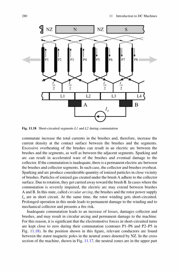
commutate increase the total currents in the brushes and, therefore, increase the
current density at the contact surface between the brushes and the segments.
Excessive overheating of the brushes can result in an electric arc between the
brushes and the segments, as well as between the adjacent segments. Sparking and
arc can result in accelerated ware of the brushes and eventual damage to the
collector. If the commutation is inadequate, there is a permanent electric arc between
the brushes and collector segments. In such case, the collector and brushes overheat.
Sparking and arc produce considerable quantity of ionized particles in close vicinity
of brushes. Particles of ionized gas created under the brush A adhere to the collector
surface. Due to rotation, they get carried away toward the brush B. In cases where the
commutation is severely impaired, the electric arc may extend between brushes
A and B. In this state, called circular arcing, the brushes and the rotor power supplyIa are in short circuit. At the same time, the rotor winding gets short-circuited.
Prolonged operation in this mode leads to permanent damage to the winding and to
mechanical collector and presents a fire risk.
Inadequate commutation leads to an increase of losses, damages collector and
brushes, and may result in circular arcing and permanent damage to the machine.
For this reason, it is significant that the electromotive forces in short-circuited turns
are kept close to zero during their commutation (contours P1–P6 and P2–P5 in
Fig. 11.18). In the position shown in this figure, relevant conductors are found
between the stator magnetic poles in the neutral zones denoted by NZ. In the cross
section of the machine, shown in Fig. 11.17, the neutral zones are in the upper part
Fig. 11.18 Short-circuited segments L1 and L2 during commutation
280 11 Introduction to DC Machines
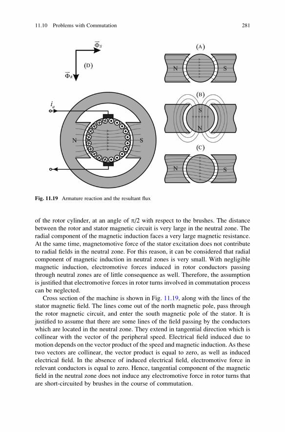
of the rotor cylinder, at an angle of p/2 with respect to the brushes. The distance
between the rotor and stator magnetic circuit is very large in the neutral zone. The
radial component of the magnetic induction faces a very large magnetic resistance.
At the same time, magnetomotive force of the stator excitation does not contribute
to radial fields in the neutral zone. For this reason, it can be considered that radial
component of magnetic induction in neutral zones is very small. With negligible
magnetic induction, electromotive forces induced in rotor conductors passing
through neutral zones are of little consequence as well. Therefore, the assumption
is justified that electromotive forces in rotor turns involved in commutation process
can be neglected.
Cross section of the machine is shown in Fig. 11.19, along with the lines of the
stator magnetic field. The lines come out of the north magnetic pole, pass through
the rotor magnetic circuit, and enter the south magnetic pole of the stator. It is
justified to assume that there are some lines of the field passing by the conductors
which are located in the neutral zone. They extend in tangential direction which is
collinear with the vector of the peripheral speed. Electrical field induced due to
motion depends on the vector product of the speed and magnetic induction. As these
two vectors are collinear, the vector product is equal to zero, as well as induced
electrical field. In the absence of induced electrical field, electromotive force in
relevant conductors is equal to zero. Hence, tangential component of the magnetic
field in the neutral zone does not induce any electromotive force in rotor turns that
are short-circuited by brushes in the course of commutation.
Fig. 11.19 Armature reaction and the resultant flux
11.10 Problems with Commutation 281
Conductors P3, P4, P7, and P8 are in the zones of magnetic poles, where
significant component of the radial magnetic induction is present; thus, the induced
electromotive forces in these conductors are proportional to the speed of rotation,
magnetic induction, and length of the conductors. The conductors of the turn P3–P8
are not below the same magnetic pole, and the electromotive forces induced in these
conductors are of opposite directions. Yet, the way of connecting them in series
(Fig. 11.18) leads to actual adding of their electromotive forces. Neglecting the
voltage drop on resistances, the voltage which appears across segments L2 and L3
is double the electromotive force induced in one conductor.
Commutation without excessive short circuit currents and with no sparks
requires that DC machine has sufficiently wide neutral zone between the stator
magnetic poles where the magnetic induction is close to zero. The way of
connecting the rotor conductors to the commutator segments must ensure that all
the rotor turns involved by the commutation process and short-circuited by the
brushes have their conductors in the neutral zone. The short circuit is created by
the brushes during intervals when they touch two adjacent segments. Therefore,
angular width of the stator magnetic poles should be less than p in order to allow for
two neutral zones between the poles. As a consequence, one part of rotor conductors
will always be in the neutral zone, where the magnetic induction has very low
value. Increasing the width of neutral zones reduces the problems associated with
commutation. At the same time, it reduces the number of rotor conductors which
are encircled by the stator magnetic field and which contribute to the electrome-
chanical conversion and torque generation.
Question (11.1): In Fig. 11.18, short-circuited turns P2–P5 and P1–P6 contain the
conductors placed at the edges of neutral zones, in the vicinity of magnetic poles.
Discuss the risk that, due to vicinity of magnetic poles, electromotive forces are
induced in short-circuited windings.
Answer (11.1): Figure 11.18 is drawn in the way that conductors P1, P2, P5, and P6
are at the edges of neutral zones, in the vicinity of magnetic poles. It is justified to
expect that, at this position, the radial component ofmagnetic induction is higher than
in themiddle of the neutral zone. Conductors P2 and P5make one turn which is short-
circuited by the brush B (Fig. 11.18). They are laid at the edges of the north magnetic
pole, symmetrically with respect to the pole. Vicinity of the magnetic pole contri-
butes to an increased magnetic induction. Because of the symmetry, in positions
where conductors P2 and P5 are placed, radial component of the magnetic induction
has the same value. For this reason, the electromotive forces induced in conductors P2
and P5 are of equal amplitude and direction. Conductors P2 and P5 are series
connected and make short-circuited turn P2–P5. Connections of conductors P2 and
P5 are such that their electromotive forces subtract and cancel. Therefore, the
electromotive force of the turn P2–P5 in position shown in Fig. 11.18 is equal to
zero. This is due to the fact that conductors P2 and P5 are symmetrical with respect
to the north magnetic pole. In all cases where short-circuited conductors, such as P2
and P5, come at the very edge of the neutral zone, in close vicinity of the stator
magnetic poles, it is possible to have considerable electromotive forces induced
282 11 Introduction to DC Machines
in such conductors. Yet, their symmetrical placement with respect to the pole ensures
cancelation of their electromotive forces. The electromotive force in short-circuited
turn P2–P5 is equal to zero. The same conclusion can be drawn for conductors P1
and P6.
11.11 Rotor Magnetic Field
Maintaining low intensities of the magnetic induction in neutral zones is hindered
by the presence of the rotor magnetomotive force. Figure 11.19 shows a simplified
presentation of the stator field, which propagates horizontally (a), and the rotor
field, created by the current sheet, which propagates in vertical direction (b). It can
be concluded that the rotor currents create the rotor flux which has its north and
south poles in neutral zones, in the area comprising the rotor conductors involved in
commutation and short-circuited by the brushes. The resultant magnetic field of the
machine is the sum of the stator and the rotor field. It can be presented in the way
shown in Fig. 11.19c. The stator and rotor fluxes can be represented by the two
mutually orthogonal vectors designated by FS and FR.
Rotor of DCmachine is also called armature, owing to the appearance of the rotorconductors which are shown in Fig. 11.5b. In the relevant literature, the term inductis also used to designate rotor of DC machines. In rotor conductors, electromotive
forces are induced, proportional to the angular speed of rotation and to the stator flux,hence the term induct.Electrical current Ia fed to the brushes is often called armaturecurrent while the voltage Ua between the brushes A and B is called armaturevoltage. The magnetomotive force and flux created by the rotor currents are called
reaction of induct or armature reaction. The term reaction is used due to the fact thatthe rotor electromotive force comes as a consequence of the stator flux. At the same
time, the rotor currents get affected by this electromotive force. Since the rotor
currents create the rotor flux, such flux is considered to be a reaction to the excitationcoming from the stator. In a way, the stator flux induces electromotive forces in rotor
conductors and affects the rotor current. For this reason, the stator is also called
inductor.The rotor flux (i.e., armature flux) is relatively small. The lines of the rotor field
come out of the rotor magnetic circuit and enter a very large air gap in neutral
zones. Therefore, the rotor flux passes through regions of very low permeability
(mo) and very high magnetic resistance. For this reason, the value of magnetic
induction in neutral zone is relatively small. Nevertheless, even a relatively small
field in neutral zone may have undesirable influence on commutation. The presence
of magnetic induction in neutral zone results in induced electromotive forces in
rotor conductors passing through the neutral zone. These conductors are involved
in the process of commutation. The turns made of such conductors are connected
to adjacent collector segments, and they get short-circuited by the brushes. Short-
circuited loop created in the prescribed way involves the rotor conductors, collector
segments, and brushes. Induced electromotive forces create short circuit currents
11.11 Rotor Magnetic Field 283
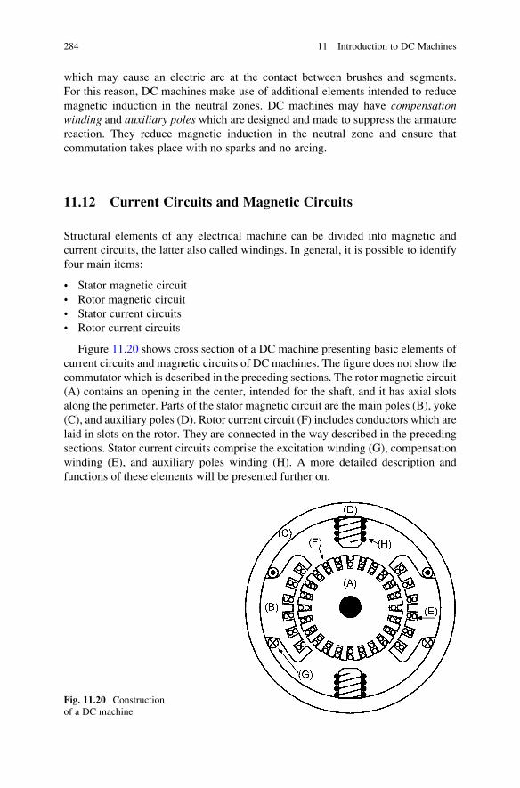
which may cause an electric arc at the contact between brushes and segments.
For this reason, DC machines make use of additional elements intended to reduce
magnetic induction in the neutral zones. DC machines may have compensationwinding and auxiliary poles which are designed and made to suppress the armature
reaction. They reduce magnetic induction in the neutral zone and ensure that
commutation takes place with no sparks and no arcing.
11.12 Current Circuits and Magnetic Circuits
Structural elements of any electrical machine can be divided into magnetic and
current circuits, the latter also called windings. In general, it is possible to identify
four main items:
• Stator magnetic circuit
• Rotor magnetic circuit
• Stator current circuits
• Rotor current circuits
Figure 11.20 shows cross section of a DC machine presenting basic elements of
current circuits and magnetic circuits of DC machines. The figure does not show the
commutator which is described in the preceding sections. The rotor magnetic circuit
(A) contains an opening in the center, intended for the shaft, and it has axial slots
along the perimeter. Parts of the stator magnetic circuit are the main poles (B), yoke
(C), and auxiliary poles (D). Rotor current circuit (F) includes conductors which are
laid in slots on the rotor. They are connected in the way described in the preceding
sections. Stator current circuits comprise the excitation winding (G), compensation
winding (E), and auxiliary poles winding (H). A more detailed description and
functions of these elements will be presented further on.
Fig. 11.20 Construction
of a DC machine
284 11 Introduction to DC Machines
11.13 Magnetic Circuits
The stator magnetic circuit contains the main poles, auxiliary poles, and yoke.
The main poles direct the stator flux, also called excitation flux. Starting from the
north magnetic pole of the stator, the flux passes through the air gap, goes through
the rotor magnetic circuit, makes another passage through the air gap, enters the
south magnetic pole of the stator, and then, via yoke, returns to the north pole.
Within the stator magnetic poles, the flux does not change the course and direction;
thus, the magnetic induction in the stator iron is constant. For that reason, there are
no losses in iron. The stator magnetic circuit does not have to be laminated, that is,it does not have to be made by stacking iron sheets. Instead, it can be made of solid
iron. The auxiliary stator poles are used to reduce the magnetic induction in the
neutral zone, which will be explained later.
The rotor magnetic circuit is of cylindrical shape. The rotor flux does not move
with respect to the stator. It remains still with respect to the stator and the stator flux.
The rotor revolves in magnetic field created by the stator and rotor windings. As a
consequence, direction of the magnetic field relative to the rotor magnetic circuit
varies as the rotor turns. Namely, observer that revolves with the rotor experiences
revolving magnetic field. As the field pulsates with respect to the rotor magnetic
circuit, there are eddy currents and iron losses in the rotor. The frequency of the
field pulsations depends on the rotor speed. Variable magnetic field produces both
hysteresis and eddy current losses in rotor iron. In order to reduce these losses, the
rotor is built by stacking iron sheets (lamination). The shape of these sheets is given
in Fig. 11.20. Along the rotor perimeter, there are slots where the rotor conductors
are placed. At the center of the rotor sheets, there is a round opening intended for
fastening the shaft. Cylindrical magnetic circuit of the rotor is formed by stacking a
large number of iron sheets of thickness less than 1 mm.
11.14 Current Circuits
Current circuits of the stator include the excitation winding, compensation wind-
ing, and winding of the auxiliary poles. The excitation winding has Nf turns around
the main poles. Excitation current creates the magnetomotive force of excitation
Ff ¼ NfIf. All the quantities and parameters related to the excitation winding have
the subscript f for field. Namely, the excitation winding provides the magnetic field
of DC machine. Dividing the magnetomotive force by magnetic resistance of the
magnetic circuit, one obtains the stator fluxFf, also called excitation flux. This flux is
equal to the surface integral of magnetic induction B over cross section of the main
poles. At the same time, it is equal to the surface integral of the magnetic induction
over the surface extending in the air gap below the main poles. In Figs. 11.19 and
11.20, the excitation flux is directed from left to right and passes twice through
the air gap of width d. By neglecting HFe and the magnetic voltage drop in iron, the
11.14 Current Circuits 285
magnetic induction in the air gap below the main poles can be estimated as
B ¼ moNfIf/(2d). Therefore, one can change the excitation flux Ff by varying the
excitation current. In addition to excitation winding, stator has compensation wind-
ing and winding of auxiliary poles.
Compensation winding consists of conductors laid in slots made on the inner
side of the main poles of the stator. This winding is connected in such way that its
conductors carry electrical current Ia/2, the same current that is carried by rotor
conductors. Direction of the current in conductors pertaining to compensation
winding is opposite to direction of rotor currents. Since conductors of the rotor
winding and those of the compensation windings are in close vicinity, their magne-
tomotive forces mutually cancel due to opposite directions of their electrical
currents. Therefore, current in the compensation winding compensates and cancels
the magnetomotive force of the rotor. This is done in order to reduce the magnetic
induction in the neutral zone and to avoid short circuit currents in rotor turns
involved in the process of commutation. The compensation winding cancels the
magnetomotive force of all the rotor conductors located under the main stator poles.
This does not include all the rotor conductors, as some of them are found in neutral
zones, away from the main poles. The magnetomotive force of these conductors is
not fully compensated by action of the compensation winding. Therefore, the
auxiliary poles are also built and placed against neutral zones with the purpose to
restrain the magnetic induction in these zones. Auxiliary poles have corresponding
winding.
Winding of auxiliary poles has turns around the auxiliary poles magnetic core,
denoted by (D) in Fig. 11.20. The air gap below the auxiliary poles is considerably
wider compared to the air gap below main magnetic poles. This is done to increase
the magnetic resistance encountered by the armature reaction. Current in the
winding of the auxiliary poles is made proportional to the rotor current. Direction
of this current and the number of turns are adjusted to achieve compensation of the
magnetomotive force of the rotor which has not been compensated by action of
the compensation winding. By joint action of the compensation winding and
auxiliary poles, it is possible to control and suppress the magnetic induction in
neutral zones, that is, below auxiliary poles. Essentially, the magnetic induction
in the neutral zones should be reduced to a value close to zero. Detailed analysis of
the process of commutation is not included in this book. Further study shows that
the stress and ware of the brushes and collector segments is reduced in cases with
linear commutation, where the current in short-circuited turns involved in commu-
tation process varies from þIa/2 to �Ia/2 in linear fashion. Prerequisite for linear
commutation is establishing magnetic induction in neutral zones which has a very
small value that varies in proportion to armature current Ia. Detailed analysis of theprocess of commutation and method of designing the compensation winding and
the winding of auxiliary poles are beyond the scope of this book.
Rotor winding is formed by connecting rotor conductors which are placed in
corresponding slots to the collector segments in the manner prescribed earlier. With
NR rotor conductors connected to segments, there are two parallel branches between
brushes A and B at each instant, each branch having NR/2 conductors. As stated
286 11 Introduction to DC Machines
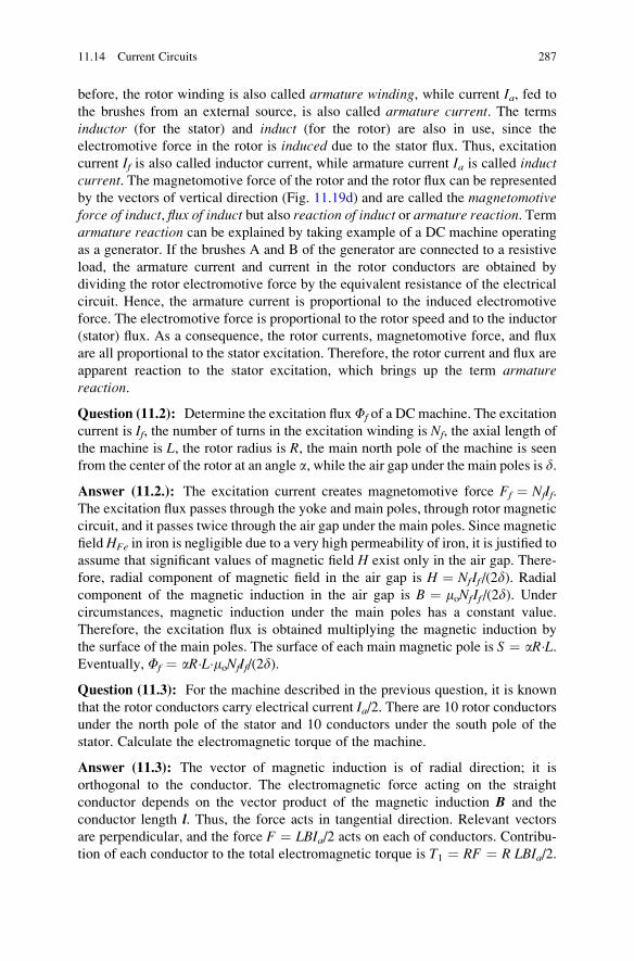
before, the rotor winding is also called armature winding, while current Ia, fed to
the brushes from an external source, is also called armature current. The terms
inductor (for the stator) and induct (for the rotor) are also in use, since the
electromotive force in the rotor is induced due to the stator flux. Thus, excitation
current If is also called inductor current, while armature current Ia is called inductcurrent. The magnetomotive force of the rotor and the rotor flux can be represented
by the vectors of vertical direction (Fig. 11.19d) and are called the magnetomotiveforce of induct, flux of induct but also reaction of induct or armature reaction. Termarmature reaction can be explained by taking example of a DC machine operating
as a generator. If the brushes A and B of the generator are connected to a resistive
load, the armature current and current in the rotor conductors are obtained by
dividing the rotor electromotive force by the equivalent resistance of the electrical
circuit. Hence, the armature current is proportional to the induced electromotive
force. The electromotive force is proportional to the rotor speed and to the inductor
(stator) flux. As a consequence, the rotor currents, magnetomotive force, and flux
are all proportional to the stator excitation. Therefore, the rotor current and flux are
apparent reaction to the stator excitation, which brings up the term armaturereaction.
Question (11.2): Determine the excitation fluxFf of a DC machine. The excitation
current is If, the number of turns in the excitation winding is Nf, the axial length of
the machine is L, the rotor radius is R, the main north pole of the machine is seen
from the center of the rotor at an angle a, while the air gap under the main poles is d.
Answer (11.2.): The excitation current creates magnetomotive force Ff ¼ NfIf.The excitation flux passes through the yoke and main poles, through rotor magnetic
circuit, and it passes twice through the air gap under the main poles. Since magnetic
field HFe in iron is negligible due to a very high permeability of iron, it is justified to
assume that significant values of magnetic field H exist only in the air gap. There-
fore, radial component of magnetic field in the air gap is H ¼ NfIf /(2d). Radialcomponent of the magnetic induction in the air gap is B ¼ moNfIf /(2d). Undercircumstances, magnetic induction under the main poles has a constant value.
Therefore, the excitation flux is obtained multiplying the magnetic induction by
the surface of the main poles. The surface of each main magnetic pole is S ¼ aR�L.Eventually, Ff ¼ aR�L�moNfIf/(2d).
Question (11.3): For the machine described in the previous question, it is known
that the rotor conductors carry electrical current Ia/2. There are 10 rotor conductorsunder the north pole of the stator and 10 conductors under the south pole of the
stator. Calculate the electromagnetic torque of the machine.
Answer (11.3): The vector of magnetic induction is of radial direction; it is
orthogonal to the conductor. The electromagnetic force acting on the straight
conductor depends on the vector product of the magnetic induction B and the
conductor length l. Thus, the force acts in tangential direction. Relevant vectors
are perpendicular, and the force F ¼ LBIa/2 acts on each of conductors. Contribu-
tion of each conductor to the total electromagnetic torque is T1 ¼ RF ¼ R LBIa/2.
11.14 Current Circuits 287
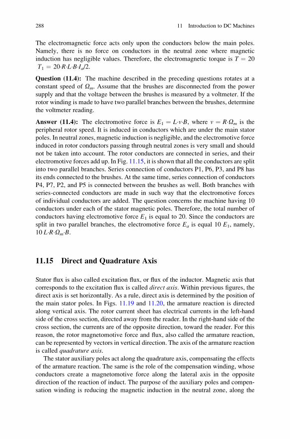
The electromagnetic force acts only upon the conductors below the main poles.
Namely, there is no force on conductors in the neutral zone where magnetic
induction has negligible values. Therefore, the electromagnetic torque is T ¼ 20
T1 ¼ 20�R�L�B�Ia/2.Question (11.4): The machine described in the preceding questions rotates at a
constant speed of Om. Assume that the brushes are disconnected from the power
supply and that the voltage between the brushes is measured by a voltmeter. If the
rotor winding is made to have two parallel branches between the brushes, determine
the voltmeter reading.
Answer (11.4): The electromotive force is E1 ¼ L�v�B, where v ¼ R�Om is the
peripheral rotor speed. It is induced in conductors which are under the main stator
poles. In neutral zones, magnetic induction is negligible, and the electromotive force
induced in rotor conductors passing through neutral zones is very small and should
not be taken into account. The rotor conductors are connected in series, and their
electromotive forces add up. In Fig. 11.15, it is shown that all the conductors are split
into two parallel branches. Series connection of conductors P1, P6, P3, and P8 has
its ends connected to the brushes. At the same time, series connection of conductors
P4, P7, P2, and P5 is connected between the brushes as well. Both branches with
series-connected conductors are made in such way that the electromotive forces
of individual conductors are added. The question concerns the machine having 10
conductors under each of the stator magnetic poles. Therefore, the total number of
conductors having electromotive force E1 is equal to 20. Since the conductors are
split in two parallel branches, the electromotive force Ea is equal 10 E1, namely,
10 L�R�Om�B.
11.15 Direct and Quadrature Axis
Stator flux is also called excitation flux, or flux of the inductor. Magnetic axis that
corresponds to the excitation flux is called direct axis. Within previous figures, the
direct axis is set horizontally. As a rule, direct axis is determined by the position of
the main stator poles. In Figs. 11.19 and 11.20, the armature reaction is directed
along vertical axis. The rotor current sheet has electrical currents in the left-hand
side of the cross section, directed away from the reader. In the right-hand side of the
cross section, the currents are of the opposite direction, toward the reader. For this
reason, the rotor magnetomotive force and flux, also called the armature reaction,
can be represented by vectors in vertical direction. The axis of the armature reaction
is called quadrature axis.The stator auxiliary poles act along the quadrature axis, compensating the effects
of the armature reaction. The same is the role of the compensation winding, whose
conductors create a magnetomotive force along the lateral axis in the opposite
direction of the reaction of induct. The purpose of the auxiliary poles and compen-
sation winding is reducing the magnetic induction in the neutral zone, along the
288 11 Introduction to DC Machines
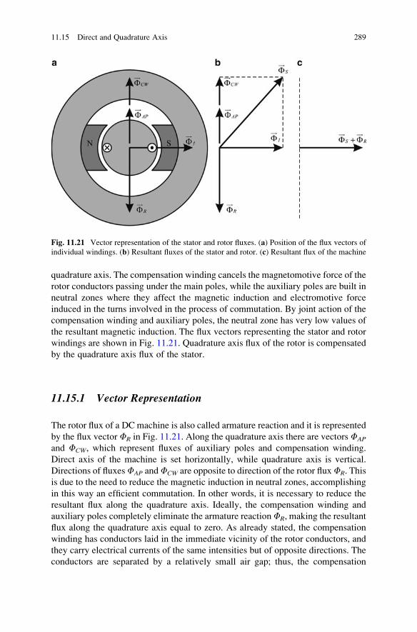
quadrature axis. The compensation winding cancels the magnetomotive force of the
rotor conductors passing under the main poles, while the auxiliary poles are built in
neutral zones where they affect the magnetic induction and electromotive force
induced in the turns involved in the process of commutation. By joint action of the
compensation winding and auxiliary poles, the neutral zone has very low values of
the resultant magnetic induction. The flux vectors representing the stator and rotor
windings are shown in Fig. 11.21. Quadrature axis flux of the rotor is compensated
by the quadrature axis flux of the stator.
11.15.1 Vector Representation
The rotor flux of a DC machine is also called armature reaction and it is represented
by the flux vector FR in Fig. 11.21. Along the quadrature axis there are vectors FAP
and FCW, which represent fluxes of auxiliary poles and compensation winding.
Direct axis of the machine is set horizontally, while quadrature axis is vertical.
Directions of fluxes FAP andFCW are opposite to direction of the rotor fluxFR. This
is due to the need to reduce the magnetic induction in neutral zones, accomplishing
in this way an efficient commutation. In other words, it is necessary to reduce the
resultant flux along the quadrature axis. Ideally, the compensation winding and
auxiliary poles completely eliminate the armature reactionFR, making the resultant
flux along the quadrature axis equal to zero. As already stated, the compensation
winding has conductors laid in the immediate vicinity of the rotor conductors, and
they carry electrical currents of the same intensities but of opposite directions. The
conductors are separated by a relatively small air gap; thus, the compensation
Fig. 11.21 Vector representation of the stator and rotor fluxes. (a) Position of the flux vectors of
individual windings. (b) Resultant fluxes of the stator and rotor. (c) Resultant flux of the machine
11.15 Direct and Quadrature Axis 289
winding efficiently cancels the magnetomotive force created by rotor conductors
that are passing below the main poles. All the remaining rotor conductors are in
neutral zones, between the main poles, out of the reach of the main poles, passing
against the auxiliary poles. The action of the auxiliary poles is intended for further
reduction of the magnetic field in neutral zones.
11.15.2 Resultant Fluxes
Figure 11.21a shows vectors representing the fluxes of individual stator and rotor
windings. Part (b) of the figure shows the resultant flux vectors. The rotor has only
one winding, the armature winding. Therefore, the resultant rotor flux is equal to
the armature reaction FR. The stator has three windings, the excitation winding, the
compensation winding, and the winding on auxiliary poles. The resultant stator flux
FS is equal to the sum of the three fluxes: the excitation flux, the flux of compensa-
tion winding, and the flux of auxiliary poles.
11.15.3 Resultant Flux of the Machine
Resultant flux of the machine is equal to the vector sum of the fluxes in all the
windings of the machine. Therefore, the resultant flux vector of the machine is
equal to the sum of the resultant stator flux FS and the rotor flux FR. In cases where
fluxes FAP and FCW compensate the armature reaction in full, the resultant flux
along the quadrature axis is equal to zero, while the resultant flux along the direct
axis is equal the excitation flux Ff, as shown in Fig. 11.21c.
Question (11.5): Figure 11.21 shows the case when the compensation winding and
auxiliary poles eliminate the rotor flux FR in full. By adding these two fluxes, one
obtains the stator flux along the quadrature axis FAP + FCW which has the same
amplitude as the rotor flux FR, but it has the opposite direction. For this reason,
the total flux of the machine along the quadrature axis is equal to zero. From
previous chapters, it is known that the electromagnetic torque of the machine is
determined by the vector product of the stator and rotor fluxes. Does the fact that
equivalent quadrature flux of the machine equals zero leads to conclusion that the
electromagnetic torque of the machine is equal to zero as well?
Answer (11.5): It is necessary to note that the electromagnetic torque depends on
the vector product of vectors FR and FS. Vector FR represents the flux created by
all the rotor windings, while vector FS represents the flux created by all the stator
windings. In the case of a DC machine, the rotor has only one winding, the
armature winding, and the flux FR is equal to the armature reaction flux. The
stator has three windings. Therefore, the vector FS represents the sum of the fluxes
in these three stator windings, namely, the excitation winding, the compensation
290 11 Introduction to DC Machines
winding, and the winding of auxiliary poles. Electrical currents in conductors of
the compensation winding and the winding of auxiliary poles create a quadrature
component of the stator flux. In the considered case, the compensation winding and
the winding of auxiliary poles create the flux along the quadrature axis which is of
the same amplitude as the rotor flux but of the opposite direction. The sum of the
fluxes created by the compensation winding and the auxiliary poles is �FR.
Therefore, the resultant flux of the machine in quadrature axis is equal to zero.
It is necessary to notice that the resultant flux of the machine comes as the sum of
the fluxes of all the machine windings, residing on both stator and rotor. Although
the resultant flux along the quadrature axis is zero, there still exists the rotor flux
along the quadrature axis. For that reason, there still exists the possibility for the
machine to generate the electromagnetic torque. The torque is determined by
the vector product of the stator and rotor flux vectors. It depends on flux vectors
FR and FS, shown in Fig. 11.21b. The angle between these two flux vectors is not
equal to p/2, but the sine of this angle has a non zero value. The torque is
determined by the product of amplitudes FR and FS and the sine of the angle
between them. Therefore, the torque assumes a nonzero value in the case under
consideration. The torque can be calculated as the product of the direct component
of the stator flux Ff and quadrature component of the rotor flux FR, both different
than zero in the considered case. Therefore, despite the fact that the resultant
quadrature flux of the machine is equal to zero, the electromagnetic torque of the
machine is different from zero.
11.16 Electromotive Force and Electromagnetic Torque
Further study of DC machines requires the expressions for calculating the
electromotive force and electromagnetic torque from the machine flux, current,
and speed. For purposes of modeling, deriving the steady-state equivalent schemes,
and constructing mechanical characteristics, it is necessary to derive the torque
expression and the electromotive force expression for DC machines. The electro-
motive force Ea in armature winding is also called the rotor electromotive force and
denoted by Ea, and it can be measured between the brushes A and B in conditions
where the armature current Ia is equal to zero (no load condition). The electromag-
netic torque and electromotive force should be expressed in terms of the armature
current, excitation flux, angular speed of the rotor, and the machine parameters.
11.16.1 Electromotive Force in Armature Winding
In each of the rotor conductors passing under the main poles of the stator, there is an
induced electromotive force E1 ¼ R�Om�B�L, where Om is angular speed of the
rotor, R is the rotor radius, L is length of the rotor cylinder, while B is the radial
11.16 Electromotive Force and Electromagnetic Torque 291
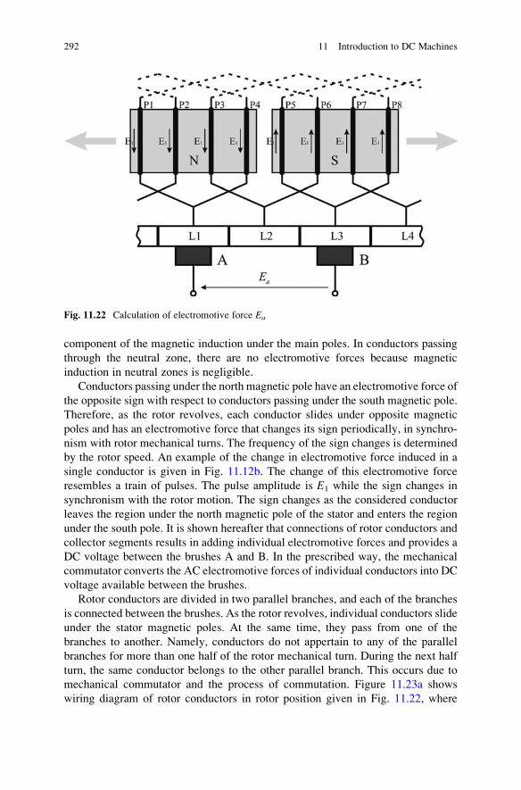
component of the magnetic induction under the main poles. In conductors passing
through the neutral zone, there are no electromotive forces because magnetic
induction in neutral zones is negligible.
Conductors passing under the north magnetic pole have an electromotive force of
the opposite sign with respect to conductors passing under the south magnetic pole.
Therefore, as the rotor revolves, each conductor slides under opposite magnetic
poles and has an electromotive force that changes its sign periodically, in synchro-
nism with rotor mechanical turns. The frequency of the sign changes is determined
by the rotor speed. An example of the change in electromotive force induced in a
single conductor is given in Fig. 11.12b. The change of this electromotive force
resembles a train of pulses. The pulse amplitude is E1 while the sign changes in
synchronism with the rotor motion. The sign changes as the considered conductor
leaves the region under the north magnetic pole of the stator and enters the region
under the south pole. It is shown hereafter that connections of rotor conductors and
collector segments results in adding individual electromotive forces and provides a
DC voltage between the brushes A and B. In the prescribed way, the mechanical
commutator converts the AC electromotive forces of individual conductors into DC
voltage available between the brushes.
Rotor conductors are divided in two parallel branches, and each of the branches
is connected between the brushes. As the rotor revolves, individual conductors slide
under the stator magnetic poles. At the same time, they pass from one of the
branches to another. Namely, conductors do not appertain to any of the parallel
branches for more than one half of the rotor mechanical turn. During the next half
turn, the same conductor belongs to the other parallel branch. This occurs due to
mechanical commutator and the process of commutation. Figure 11.23a shows
wiring diagram of rotor conductors in rotor position given in Fig. 11.22, where
Fig. 11.22 Calculation of electromotive force Ea
292 11 Introduction to DC Machines
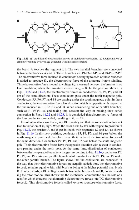
the brush A touches the segment L1. The two parallel branches are connected
between the brushes A and B. These branches are P1-P6-P3-P8 and P4-P7-P2-P5.
The electromotive force induced in conductors belonging to each of these branches
is added to produce Ea, the electromotive force of the armature (rotor) winding.
This electromotive force is equal to voltageUa, measured between the brushes in no
load condition, when the armature current is Ia ¼ 0. In the position shown in
Figs. 11.22 and 11.23, the electromotive forces in conductors P1, P2, P3, and P4
are of the same direction. These conductors pass under the north magnetic pole.
Conductors P5, P6, P7, and P8 are passing under the south magnetic pole. In these
conductors, the electromotive force has direction which is opposite with respect to
the one induced in P1, P2, P3, and P4. When considering one of parallel branches,
such as P1-P6-P3-P8, and taking into account the way of making their series
connection in Figs. 11.22 and 11.23, it is concluded that electromotive forces of
the four conductors are added, resulting in Ea ¼ 4E1.
It is of interest to show that Ea is a DC quantity and that the rotor motion does not
lead to variation of Ea sign. When the rotor turns by p/4 with respect to position in
Fig. 11.22, the brushes A and B get in touch with segments L2 and L4, as shown
in Fig. 11.16. In this new position, conductors P3, P4, P5, and P6 pass below the
north magnetic pole and therefore have their induced electromotive forces of
the same direction. Conductors P7, P8, P1, and P2 pass below the south magnetic
pole. Their electromotive forces have the opposite direction with respect to conduc-
tors passing under the north pole. At the same time, distribution of conductors
between the two parallel branches changes. According to Fig. 11.16, conductors P3,
P8, P5, and P2 make one parallel branch, while conductors P6, P1, P4, and P7 make
the other parallel branch. The figure shows that the conductors are connected in
the way that their electromotive forces are actually added; thus, the electromotive
force Ea remains equal to 4E1, with brush A being at the higher potential than brush
B. In other words, a DC voltage exists between the brushes A and B, notwithstand-
ing the rotor motion. This shows that the mechanical commutator has the role of a
rectifier which converts the alternating electromotive forces into DC electromotive
force Ea. This electromotive force is called rotor or armature electromotive force.
Fig. 11.23 (a) Addition of electromotive forces of individual conductors. (b) Representation of
armature winding by a voltage generator with internal resistance
11.16 Electromotive Force and Electromagnetic Torque 293
If the brushes A and B are connected to an external resistor or other consumer of
electrical energy which operates with DC currents, the machine shown in Fig. 11.23
will run as a generator, supplying electrical energy to the consumer. It will be shown
later that in such case, it is required to drive the rotor by an external torque obtained
from a hydro turbine, steam turbine, or internal combustion motor. The armature
winding then represents a voltage generator whose terminals are available at brushes
A and B and which produces a DC voltage Ua. The equivalent voltage generator
is shown in Fig. 11.23b. Under no load conditions, voltage between the brushes is
equal to the electromotive force Ea ¼ 4E1 ¼ 4ROmBL. Internal resistance of the
equivalent voltage generator Ra includes resistance of the brushes A and B, resis-
tance of rotor conductors connected in two parallel branches, and a relatively small
resistance of collector segments. It can be determined by measuring resistance
between the brushes in conditions where the rotor speed is equal to zero (Om ¼ 0).
The electromotive force is then equal to zero, and the equivalent voltage source is
reduced to internal resistance Ra. The value of Ra can be calculated for DC machine
with eight rotor conductors, divided in two parallel branches with four conductor
each, as shown in Fig. 11.23. If resistance of one rotor conductor is R1 while
the equivalent resistance of the brushes and collector is DR, then the internal
resistance of the equivalent source is Ra ¼ 2R1 þDR. Previous considerations
show that the armature winding of DC machine can be represented by a voltage
generator having no load electromotive force Ea and internal resistance Ra.
11.16.2 Torque Generation
It is required to determine relation between the electromagnetic torque, excitation
flux, and armature current. The excitation flux from the main poles passes to the
rotor magnetic circuit via air gap, where the magnetic induction is of radial
direction. The surface separating internal side of the main pole from the air gap is
of the form of a bent rectangle which represents a sector of the cylinder. The surface
of this sector is S ¼ WL, where L is length of the machine while W ¼ aR is
the width of the main pole, measured along its internal side which faces the air
gap. The width W is one section of the circle having the radius R. To an observer
positioned at the rotor center, the surface S is seen at the angle a. Magnetic
induction B in the air gap below the main poles is equal to the ratio of flux Ff and
surface S. The current in rotor conductors is Ia/2, where Ia is the armature current,fed to the brushes from an external source. Figure 11.24a gives an unfolded scheme
of the rotor winding and shows forces acting upon its conductors. Part (b) of this
figure shows directions of electrical currents in rotor conductors, seen from the
collector side. At the given position of the rotor, conductors P1, P2, P3, and P4
are below the north pole and carry currents of direction �. Lines of the field of
magnetic induction come out of the main pole, denoted by N; they pass through the
air gap, come across the rotor conductors, and enter the rotor magnetic circuit.
In the considered zone below the north pole, the vector product of radial component
294 11 Introduction to DC Machines
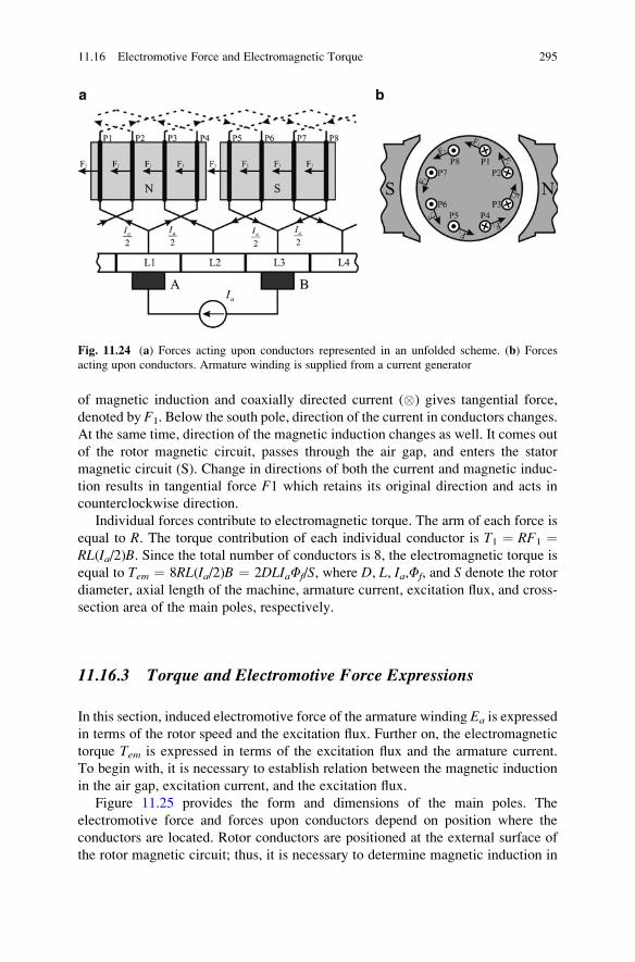
of magnetic induction and coaxially directed current (�) gives tangential force,
denoted by F1. Below the south pole, direction of the current in conductors changes.
At the same time, direction of the magnetic induction changes as well. It comes out
of the rotor magnetic circuit, passes through the air gap, and enters the stator
magnetic circuit (S). Change in directions of both the current and magnetic induc-
tion results in tangential force F1 which retains its original direction and acts in
counterclockwise direction.
Individual forces contribute to electromagnetic torque. The arm of each force is
equal to R. The torque contribution of each individual conductor is T1 ¼ RF1 ¼RL(Ia/2)B. Since the total number of conductors is 8, the electromagnetic torque is
equal to Tem ¼ 8RL(Ia/2)B ¼ 2DLIaFf/S, where D, L, Ia,Ff, and S denote the rotor
diameter, axial length of the machine, armature current, excitation flux, and cross-
section area of the main poles, respectively.
11.16.3 Torque and Electromotive Force Expressions
In this section, induced electromotive force of the armature winding Ea is expressed
in terms of the rotor speed and the excitation flux. Further on, the electromagnetic
torque Tem is expressed in terms of the excitation flux and the armature current.
To begin with, it is necessary to establish relation between the magnetic induction
in the air gap, excitation current, and the excitation flux.
Figure 11.25 provides the form and dimensions of the main poles. The
electromotive force and forces upon conductors depend on position where the
conductors are located. Rotor conductors are positioned at the external surface of
the rotor magnetic circuit; thus, it is necessary to determine magnetic induction in
Fig. 11.24 (a) Forces acting upon conductors represented in an unfolded scheme. (b) Forces
acting upon conductors. Armature winding is supplied from a current generator
11.16 Electromotive Force and Electromagnetic Torque 295
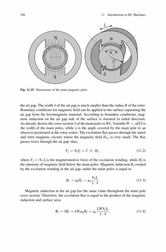
the air gap. The width d of the air gap is much smaller than the radius R of the rotor.
Boundary conditions for magnetic field can be applied to the surface separating the
air gap from the ferromagnetic material. According to boundary conditions, mag-
netic induction on the air gap side of the surface is oriented in radial direction.
As already shown, the cross-section S of themain poles isWL. VariableW ¼ aD/2 isthe width of the main poles, while a is the angle covered by the main pole to an
observer positioned at the rotor center. The excitation flux passes through the stator
and rotor magnetic circuits where the magnetic field HFe is very small. The flux
passes twice through the air gap; thus,
Ff ¼ Nf If ¼ 2 � d � Hf ; (11.2)
where Ff ¼ Nf If is the magnetomotive force of the excitation winding, while Hf is
the intensity of magnetic field below the main poles. Magnetic induction Bf created
by the excitation winding in the air gap, under the main poles is equal to
Bf ¼ m0Hf ¼ m0Nf If2 � d : (11.3)
Magnetic induction in the air gap has the same value throughout the main pole
cross section. Therefore, the excitation flux is equal to the product of the magnetic
induction and surface area
Ff ¼ SBf ¼ LWm0Hf ¼ m0LWNf If2 � d ; (11.4)
Fig. 11.25 Dimensions of the main magnetic poles
296 11 Introduction to DC Machines
where W ¼ aD/2 is the width of the main pole. Magnetic resistance along the path
of the excitation flux is equal to the ratio of magnetomotive force Ff and flux Ff.
Magnetic resistance Rm is
Rm ¼ Ff
Ff¼ 2 � d
m0 � L �W : (11.5)
Total flux of the excitation winding isCf ¼ NfFf. Inductance Lf of the excitationwinding is the ratio of the total flux and the excitation current, and it is determined
according to expression
Lf ¼cf
If¼ m0
LWN2f
2 � d ¼ N2f
Rm: (11.6)
Coefficient of proportionality between the excitation flux Ff, which represents
the flux in one turn of the excitation winding, and excitation current If is equal to
L0f ¼Ff
If¼ cf
Nf If¼ m0
LWNf
2 � d ¼ LfNf
: (11.7)
The rotor comprises a total of NR conductors, but some of them are not under
the main poles, and they pass through the neutral zone between the main poles. The
remaining rotor conductors are in the zone of the main poles, within the reach of the
magnetic induction Bf. In the neutral zone, the conductors are not subject to any
force and no electromotive force is induced in them. The rotor conductors are
evenly distributed along the machine perimeter. Below the north pole of the width
W, there are NRW/(pD) rotor conductors. The same number of conductors is found
below the south magnetic pole.
11.16.4 Calculation of Electromotive Force Ea
In the rotor conductors influenced by the field of the main poles, the induced
electromotive force E1 is
E1 ¼ Bf � L � v ¼ Bf � L � R � Om; (11.8)
where v is rotor peripheral speed, Om is angular speed of rotor rotation, and R is
radius of the rotor. Rotor conductors are connected in series in the way that the
induced electromotive forces are added. Total number of conductors containing
induced electromotive force is equal to the sum of conductors below the north and
south poles, 2NRW/(pD). Since all rotor conductors are connected in two parallel
branches, while the branch terminals are brought to brushes A and B, electromotive
11.16 Electromotive Force and Electromagnetic Torque 297
force Ea is equal to the sum of electromotive forces in one of the branches. Induced
electromotive forces exist in conductors under the main poles. Therefore, Ea is
calculated as the product of the electromotive force E1 in one conductor, and the
number of conductors positioned below one of magnetic poles,
Ea ¼ 1
2
2NRW
pD
� �E1 ¼ NRW
2pRBf LROm ¼ NR
2pLWBf
� �Om: (11.9)
By using relation (11.4) between the magnetic induction and excitation flux,
previous expression takes the form
Ea ¼ NR
2pFfOm ¼ keFfOm; (11.10)
where coefficient ke ¼ NR/(2p) is determined by the number of rotor conductors
and is called coefficient of electromotive force.
11.16.5 Calculation of Torque
Each conductor which passes through the zone of the main poles is subject to the
force
F1 ¼ LIA2Bf ¼ Ff
W � L � IA2� L ¼ Ff
W� IA2: (11.11)
The arm of the considered force is R ¼ D/2, and its contribution to the total
torque is equal to T1 ¼ F1 D/2. Since the force F1 acts only on conductors
positioned below the main poles, there are 2NRW/(pD) conductors contributing to
the torque. The sum of their contributions is
Tem ¼ 2NRW
pD
� �� T1 ¼ 2NRW
pD� D2� Ff
W� IA2
¼ NR
2p� Ff � IA ¼ km � Ff � IA;
where km ¼ NR/(2p) is the coefficient of electromagnetic torque.Equation (11.10) shows that the electromotive force of the armature winding is
determined by the product of the excitation flux and the rotor angular speed, while
(11.12) shows that the electromagnetic torque of the machine is determined by the
product of the excitation flux and the armature current.
298 11 Introduction to DC Machines
Chapter 12
Modeling and Supplying DC Machines
In this chapter, mathematical model is developed for DCmachines with excitation
windings and DC machines with permanent magnet excitation. The block dia-
gram of the model is used to provide a brief introduction to the torque control.
Steady-state equivalent circuits are derived and explained for armature and
excitation windings. These circuits are used to introduce and analyze mechanical
characteristic of separately excited DC machine and determine the steady-state
speed. The chapter provides basic elements for the control of the rotor speed.
Steady-state operation of DC generators is explained along with basic output
characteristics. Typical applications of DC machines are classified on the basis of
the speed and torque changes within the four quadrants of Tem–Om plane. On that
ground, the basic requirements are specified for the power supply of the armature
windings. The operation of switching power converter with H-bridge is briefly
explained, along with the basic notions on pulse-width modulation (PWM). The
impact of pulsed power supply on the machine operation is considered by study-
ing the ripple of the armature current. The chapter closes with an overview of most
common power converter topologies used in supplying DC machines.
Analysis of electrical and mechanical characteristics of a DC machine is based
on mathematical model. The model contains differential equations and algebraic
relations describing transient processes in the machine. In DC electrical machines,
the excitation flux is established along direct axis, while the rotor flux (armaturereaction) appears along quadrature axis. The two axes are orthogonal, and the
mutual inductance between the excitation winding and the armature windings is
S.N. Vukosavic, Electrical Machines, Power Electronics and Power Systems,
DOI 10.1007/978-1-4614-0400-2_12, # Springer Science+Business Media New York 2013
299
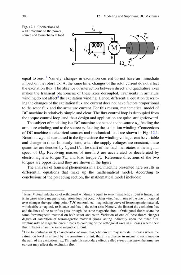
equal to zero.1 Namely, changes in excitation current do not have an immediate
impact on the rotor flux. At the same time, changes of the rotor current do not affect
the excitation flux. The absence of interaction between direct and quadrature axes
makes the transient phenomena of these axes decoupled. Transients in armature
winding do not affect2 the excitation winding. Hence, differential equation describ-
ing the changes of the excitation flux and current does not have factors proportional
to the rotor flux and the armature current. For this reason, mathematical model of
DC machine is relatively simple and clear. The flux control loop is decoupled from
the torque control loop, and their design and application are quite straightforward.
The subject of modeling is a DC machine connected to the source ua, feeding thearmature winding, and to the source uf, feeding the excitation winding. Connectionsof DC machine to electrical sources and mechanical load are shown in Fig. 12.1.
Notations ua and uf are used in the figure since the winding voltages can be variableand change in time. In steady state, when the supply voltages are constant, these
quantities are denoted by Ua and Uf. The shaft of the machine rotates at the angular
speed of Om. Revolving masses of inertia J are accelerated or decelerated by
electromagnetic torque Tem and load torque Tm. Reference directions of the two
torques are opposite, and they are shown in the figure.
The analysis of transient phenomena in a DC machine presented here results in
differential equations that make up the mathematical model. According to
conclusions of the preceding section, the mathematical model includes:
Fig. 12.1 Connections of
a DC machine to the power
source and to mechanical load
1Note: Mutual inductance of orthogonal windings is equal to zero if magnetic circuit is linear, that
is, in cases where magnetic saturation does not occur. Otherwise, flux in one of the two orthogonal
axes changes the operating point (B,H) on nonlinear magnetizing curve of ferromagnetic material,
which affects magnetic resistance and flux in the other axis. Namely, the lines of the excitation flux
and the lines of the rotor flux pass through the same magnetic circuit. Orthogonal fluxes share the
same ferromagnetic material on both stator and rotor. Variation of one of these fluxes changes
degree of saturation of ferromagnetic material (iron), acting indirectly upon the other flux.
Nonlinearity of magnetic circuit leads to coupling of the orthogonal axes in all cases where their
flux linkages share the same magnetic circuit.2 Due to nonlinear B(H) characteristic of iron, magnetic circuit may saturate. In cases where the
saturation level is altered by the armature current, there is a change in magnetic resistance on
the path of the excitation flux. Through this secondary effect, called cross saturation, the armature
current may affect the excitation flux.
300 12 Modeling and Supplying DC Machines
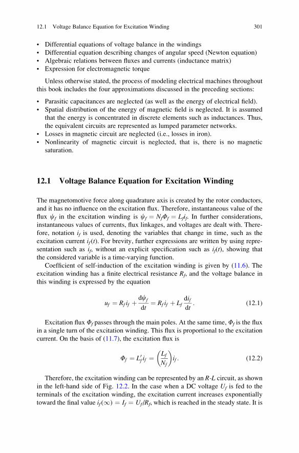
• Differential equations of voltage balance in the windings
• Differential equation describing changes of angular speed (Newton equation)
• Algebraic relations between fluxes and currents (inductance matrix)
• Expression for electromagnetic torque
Unless otherwise stated, the process of modeling electrical machines throughout
this book includes the four approximations discussed in the preceding sections:
• Parasitic capacitances are neglected (as well as the energy of electrical field).
• Spatial distribution of the energy of magnetic field is neglected. It is assumed
that the energy is concentrated in discrete elements such as inductances. Thus,
the equivalent circuits are represented as lumped parameter networks.
• Losses in magnetic circuit are neglected (i.e., losses in iron).
• Nonlinearity of magnetic circuit is neglected, that is, there is no magnetic
saturation.
12.1 Voltage Balance Equation for Excitation Winding
The magnetomotive force along quadrature axis is created by the rotor conductors,
and it has no influence on the excitation flux. Therefore, instantaneous value of the
flux cf in the excitation winding is cf ¼ NfFf ¼ Lfif. In further considerations,
instantaneous values of currents, flux linkages, and voltages are dealt with. There-
fore, notation if is used, denoting the variables that change in time, such as the
excitation current if(t). For brevity, further expressions are written by using repre-
sentation such as if, without an explicit specification such as if(t), showing that
the considered variable is a time-varying function.
Coefficient of self-induction of the excitation winding is given by (11.6). The
excitation winding has a finite electrical resistance Rf, and the voltage balance in
this winding is expressed by the equation
uf ¼ Rf if þdcf
dt¼ Rf if þ Lf
difdt
: (12.1)
Excitation flux Ff passes through the main poles. At the same time, Ff is the flux
in a single turn of the excitation winding. This flux is proportional to the excitation
current. On the basis of (11.7), the excitation flux is
Ff ¼ L0f if ¼LfNf
� �if : (12.2)
Therefore, the excitation winding can be represented by an R-L circuit, as shown
in the left-hand side of Fig. 12.2. In the case when a DC voltage Uf is fed to the
terminals of the excitation winding, the excitation current increases exponentially
toward the final value if (1) ¼ If ¼ Uf /Rf, which is reached in the steady state. It is
12.1 Voltage Balance Equation for Excitation Winding 301
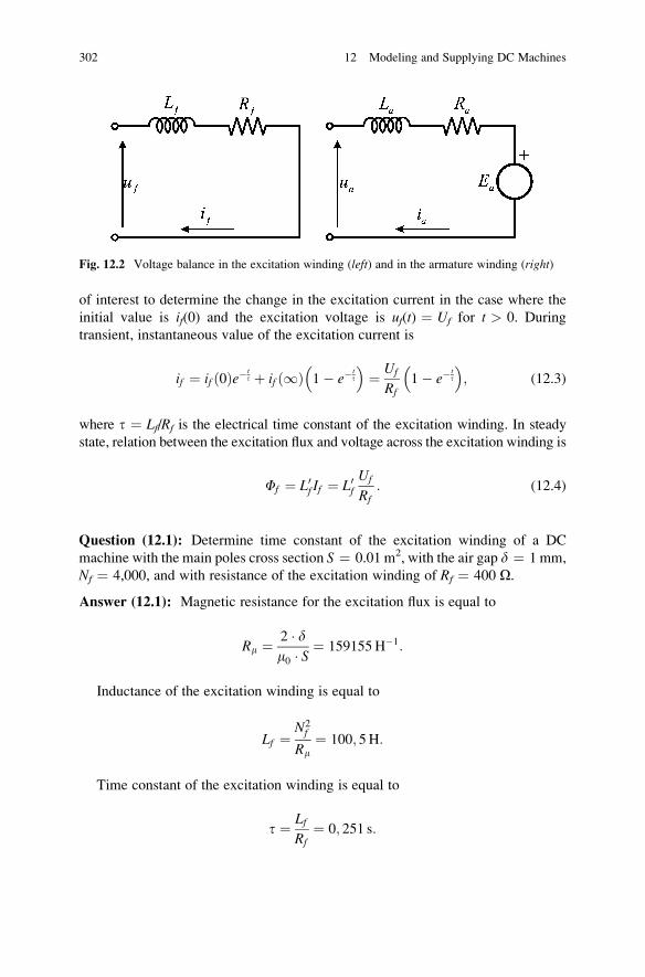
of interest to determine the change in the excitation current in the case where the
initial value is if(0) and the excitation voltage is uf(t) ¼ Uf for t > 0. During
transient, instantaneous value of the excitation current is
if ¼ if ð0Þe�tt þ if 1ð Þ 1� e�
tt
� �¼ Uf
Rf1� e�
tt
� �; (12.3)
where t ¼ Lf/Rf is the electrical time constant of the excitation winding. In steady
state, relation between the excitation flux and voltage across the excitation winding is
Ff ¼ L0f If ¼ L0fUf
Rf: (12.4)
Question (12.1): Determine time constant of the excitation winding of a DC
machine with the main poles cross section S ¼ 0.01 m2, with the air gap d ¼ 1 mm,
Nf ¼ 4,000, and with resistance of the excitation winding of Rf ¼ 400 O.
Answer (12.1): Magnetic resistance for the excitation flux is equal to
Rm ¼ 2 � dm0 � S
¼ 159155H�1:
Inductance of the excitation winding is equal to
Lf ¼N2f
Rm¼ 100; 5H:
Time constant of the excitation winding is equal to
t ¼ LfRf
¼ 0; 251 s:
Fig. 12.2 Voltage balance in the excitation winding (left) and in the armature winding (right)
302 12 Modeling and Supplying DC Machines
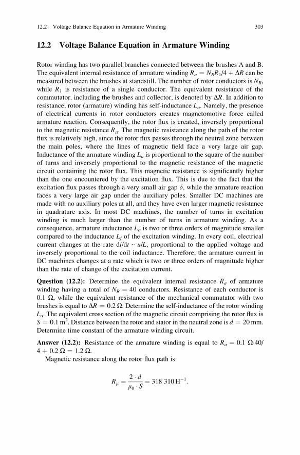
12.2 Voltage Balance Equation in Armature Winding
Rotor winding has two parallel branches connected between the brushes A and B.
The equivalent internal resistance of armature winding Ra ¼ NRR1/4 + DR can be
measured between the brushes at standstill. The number of rotor conductors is NR,
while R1 is resistance of a single conductor. The equivalent resistance of the
commutator, including the brushes and collector, is denoted by DR. In addition to
resistance, rotor (armature) winding has self-inductance La. Namely, the presence
of electrical currents in rotor conductors creates magnetomotive force called
armature reaction. Consequently, the rotor flux is created, inversely proportional
to the magnetic resistance Rm. The magnetic resistance along the path of the rotor
flux is relatively high, since the rotor flux passes through the neutral zone between
the main poles, where the lines of magnetic field face a very large air gap.
Inductance of the armature winding La is proportional to the square of the number
of turns and inversely proportional to the magnetic resistance of the magnetic
circuit containing the rotor flux. This magnetic resistance is significantly higher
than the one encountered by the excitation flux. This is due to the fact that the
excitation flux passes through a very small air gap d, while the armature reaction
faces a very large air gap under the auxiliary poles. Smaller DC machines are
made with no auxiliary poles at all, and they have even larger magnetic resistance
in quadrature axis. In most DC machines, the number of turns in excitation
winding is much larger than the number of turns in armature winding. As a
consequence, armature inductance La is two or three orders of magnitude smaller
compared to the inductance Lf of the excitation winding. In every coil, electrical
current changes at the rate di/dt ~ u/L, proportional to the applied voltage and
inversely proportional to the coil inductance. Therefore, the armature current in
DC machines changes at a rate which is two or three orders of magnitude higher
than the rate of change of the excitation current.
Question (12.2): Determine the equivalent internal resistance Ra of armature
winding having a total of NR ¼ 40 conductors. Resistance of each conductor is
0.1 O, while the equivalent resistance of the mechanical commutator with two
brushes is equal to DR ¼ 0.2 O. Determine the self-inductance of the rotor winding
La. The equivalent cross section of the magnetic circuit comprising the rotor flux is
S ¼ 0.1 m2. Distance between the rotor and stator in the neutral zone is d ¼ 20 mm.
Determine time constant of the armature winding circuit.
Answer (12.2): Resistance of the armature winding is equal to Ra ¼ 0.1 O�40/4 þ 0.2 O ¼ 1.2 O.
Magnetic resistance along the rotor flux path is
Rm ¼ 2 � dm0 � S
¼ 318 310H�1:
12.2 Voltage Balance Equation in Armature Winding 303
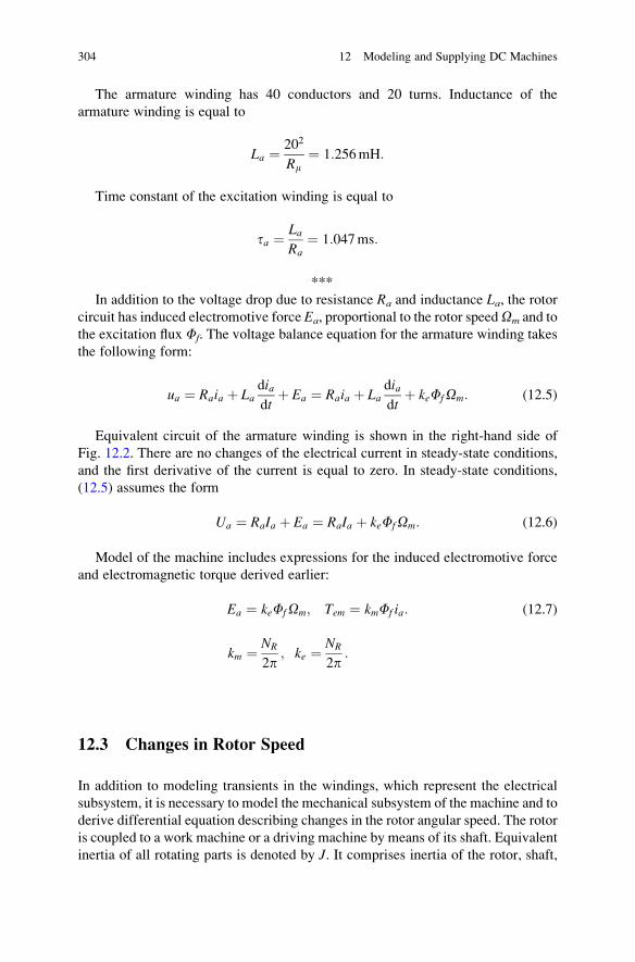
The armature winding has 40 conductors and 20 turns. Inductance of the
armature winding is equal to
La ¼ 202
Rm¼ 1:256mH:
Time constant of the excitation winding is equal to
ta ¼ LaRa
¼ 1:047ms:
***
In addition to the voltage drop due to resistance Ra and inductance La, the rotorcircuit has induced electromotive force Ea, proportional to the rotor speedOm and to
the excitation flux Ff. The voltage balance equation for the armature winding takes
the following form:
ua ¼ Raia þ Ladiadt
þ Ea ¼ Raia þ Ladiadt
þ keFfOm: (12.5)
Equivalent circuit of the armature winding is shown in the right-hand side of
Fig. 12.2. There are no changes of the electrical current in steady-state conditions,
and the first derivative of the current is equal to zero. In steady-state conditions,
(12.5) assumes the form
Ua ¼ RaIa þ Ea ¼ RaIa þ keFfOm: (12.6)
Model of the machine includes expressions for the induced electromotive force
and electromagnetic torque derived earlier:
Ea ¼ keFfOm; Tem ¼ kmFf ia: (12.7)
km ¼ NR
2p; ke ¼ NR
2p:
12.3 Changes in Rotor Speed
In addition to modeling transients in the windings, which represent the electrical
subsystem, it is necessary to model the mechanical subsystem of the machine and to
derive differential equation describing changes in the rotor angular speed. The rotor
is coupled to a work machine or a driving machine by means of its shaft. Equivalent
inertia of all rotating parts is denoted by J. It comprises inertia of the rotor, shaft,
304 12 Modeling and Supplying DC Machines
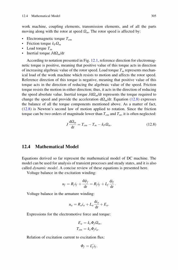
work machine, coupling elements, transmission elements, and of all the parts
moving along with the rotor at speed Om. The rotor speed is affected by:
• Electromagnetic torque Tem• Friction torque kFOm
• Load torque Tm• Inertial torque JdOm/dt
According to notation presented in Fig. 12.1, reference direction for electromag-
netic torque is positive, meaning that positive value of this torque acts in direction
of increasing algebraic value of the rotor speed. Load torque Tm represents mechan-
ical load of the work machine which resists to motion and affects the rotor speed.
Reference direction of this torque is negative, meaning that positive value of this
torque acts in the direction of reducing the algebraic value of the speed. Friction
torque resists the motion in either direction; thus, it acts in the direction of reducing
the speed absolute value. Inertial torque JdOm/dt represents the torque required to
change the speed and provide the acceleration dOm/dt. Equation (12.8) expresses
the balance of all the torque components mentioned above. As a matter of fact,
(12.8) is Newton’s second law of motion applied to rotation. Since the friction
torque can be two orders of magnitude lower than Tem and Tm, it is often neglected:
JdOm
dt¼ Tem � Tm � kFOm: (12.8)
12.4 Mathematical Model
Equations derived so far represent the mathematical model of DC machine. The
model can be used for analysis of transient processes and steady states, and it is also
called dynamic model. A concise review of these equations is presented here.
Voltage balance in the excitation winding:
uf ¼ Rf if þdcf
dt¼ Rf if þ Lf
difdt
:
Voltage balance in the armature winding:
ua ¼ Raia þ Ladiadt
þ Ea:
Expressions for the electromotive force and torque:
Ea ¼ keFfOm;
Tem ¼ keFf ia:
Relation of excitation current to excitation flux:
Ff ¼ L0f if :
12.4 Mathematical Model 305
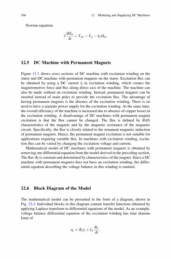
Newton equation:
JdOm
dt¼ Tem � Tm � kFOm:
12.5 DC Machine with Permanent Magnets
Figure 11.1 shows cross sections of DC machine with excitation winding on the
stator and DC machine with permanent magnets on the stator. Excitation flux can
be obtained by using a DC current If in excitation winding, which creates the
magnetomotive force and flux along direct axis of the machine. The machine can
also be made without an excitation winding. Instead, permanent magnets can be
inserted instead of main poles to provide the excitation flux. The advantage of
having permanent magnets is the absence of the excitation winding. There is no
need to have a separate power supply for the excitation winding. At the same time,
the overall efficiency of the machine is increased due to absence of copper losses in
the excitation winding. A disadvantage of DC machines with permanent magnet
excitation is that the flux cannot be changed. The flux is defined by B(H)characteristics of the magnets and by the magnetic resistance of the magnetic
circuit. Specifically, the flux is closely related to the remanent magnetic induction
of permanent magnets. Hence, the permanent magnet excitation is not suitable for
applications requiring variable flux. In machines with excitation winding, excita-
tion flux can be varied by changing the excitation voltage and current.
Mathematical model of DC machines with permanent magnets is obtained by
removing one differential equation from the model derived in the preceding section.
The flux Ff is constant and determined by characteristics of the magnet. Since a DC
machine with permanent magnets does not have an excitation winding, the differ-
ential equation describing the voltage balance in this winding is omitted.
12.6 Block Diagram of the Model
The mathematical model can be presented in the form of a diagram, shown in
Fig. 12.3. Individual blocks in this diagram contain transfer functions obtained by
applying Laplace transform to differential equations of the model. As an example,
voltage balance differential equation of the excitation winding has time domain
form of
uf ¼ Rf if þ Lfdifdt
:
306 12 Modeling and Supplying DC Machines
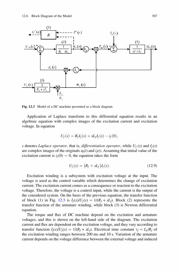
Application of Laplace transform to this differential equation results in an
algebraic equation with complex images of the excitation current and excitation
voltage. In equation
Uf ðsÞ ¼ Rf If ðsÞ þ sLf If ðsÞ � if ð0Þ;
s denotes Laplace operator, that is, differentiation operator, while Uf (s) and If (s)are complex images of the originals uf(t) and if(t). Assuming that initial value of the
excitation current is if (0) ¼ 0, the equation takes the form
Uf ðsÞ ¼ Rf þ sLf� �
If ðsÞ: (12.9)
Excitation winding is a subsystem with excitation voltage at the input. The
voltage is used as the control variable which determines the change of excitation
current. The excitation current comes as a consequence or reaction to the excitation
voltage. Therefore, the voltage is a control input, while the current is the output of
the considered system. On the basis of the previous equation, the transfer function
of block (1) in Fig. 12.3 is If (s)/Uf (s) ¼ 1/(Rf + sLf). Block (2) represents the
transfer function of the armature winding, while block (3) is Newton differential
equation.
The torque and flux of DC machine depend on the excitation and armature
voltages, and this is shown on the left-hand side of the diagram. The excitation
current and flux are dependent on the excitation voltage, and they vary according to
transfer function If(s)/Uf(s) ¼ 1/(Rf + sLf). Electrical time constant tf ¼ Lf /Rf of
the excitation winding ranges between 200 ms and 10 s. Variation of the armature
current depends on the voltage difference between the external voltage and induced
Fig. 12.3 Model of a DC machine presented as a block diagram
12.6 Block Diagram of the Model 307
electromotive force (Ua � Ea). Variation of the current dia(t)/dt is positive when
Ua � Ea � Ra ia(t) > 0; otherwise, variation of the current is negative. Time
constant of the armature winding tа ¼ Lа/Rа ranges from 1 up to 100 ms.
The excitation voltage and armature voltage are inputs to the system. They are
control variables that affect the state of DC machine. The armature current, excita-
tion current, as well as the rotor speed are state variables of the considered dynamic
system. The state variables are the reaction of the system to the external control
variables. Variables such as the armature current, excitation flux, electromagnetic
torque, and the rotor speed are the system outputs.Electromagnetic torque Tem is equal to the product of the excitation flux, armature
current, and constant km. Torque Tem represents input variable of the mechanical
subsystem, that is, control force which determines variation of the rotor speed. Speed
of rotation increases when Tem exceeds the sum of all torques resisting the
movement. When the electromagnetic torque equals the sum of resisting torques,
Tm þ kFOm, the rotor speed remains constant. If Tem < Tm þ kFOm, the rotor speed
decreases. It should be noted that block (3) of the diagram corresponds to the friction
torque kFOm. The friction torque is usually smaller than the rated torque by two
orders of magnitude. Therefore, friction is often neglected, and the transfer function
is represented by 1/(J�s).
12.7 Torque Control
Block (4) in Fig. 12.3 is denoted by R, and it does not belong to the mathematical
model of DC machine. Connections of this block are made by dotted lines. This
block illustrates the possibility of controlling the torque of the machine, which is
discussed here. DC motors are often used in motion control applications, where
they provide the means for controlling the speed and position of tools and
workpieces in automated production lines. They are also used for running elevators,
conveyors, and similar devices. In motion control tasks, electrical motors are used
to provide a variable torque Tem which should be equal to the torque reference T*,calculated within the motion controller which is not shown in the figure. The torque
reference T*is determined so as to overcome the motion resistances and ensure
desired speed and/or position. Its change depends on desired speed changes and on
forces and torques resisting the motion. The torque Tem should be as close to the
reference T* as possible. Torque control implies a set of actions and measures
conceived to maintain the electromagnetic torque Tem at the desired reference value
T*. In cases where the reference changes, controlled variable Tem should track these
changes. The torque Tem is proportional to the product of the armature current and
the flux. At the first glimpse, the torque control can be done either by changing the
flux or by changing the armature current. Yet, only the later approach is used in
practice. This is due to the fact that the flux changes are rather slow. Moreover, flux
control is not available with DC machines having permanent magnet excitation.
With DC machines having an excitation winding, the time constant of the armature
308 12 Modeling and Supplying DC Machines
winding ta is considerably smaller than the time constant of the excitation winding.
While only slow variations of the flux are possible, the current ia can be changed
quickly. Thus, regulation of the torque implies regulation of the armature current.
The speed of the torque response is defined by the speed of response of the armature
current. Starting from the voltage balance equation of the armature winding,
variation of the current is determined by equation
diadt
¼ 1
Laua � Raia � Eað Þ: (12.10)
Therefore, variations of the armature current can be accomplished by varying the
armature voltage ua. For this reason, DC motors are supplied from static power
converters, power electronic devices that provide variable armature voltage. For the
purpose of current control, it is necessary to measure the armature current and
compare it to the reference in order to establish the error Dia ¼ i* � ia. If the
armature current is below the reference (Dia > 0), armature voltage should be
increased in order to obtain dia/dt > 0. From (12.10), it can be concluded that
increasing armature voltage leads to increasing armature current; thus, error Dia isreduced. In a like manner, if the current is too high (Dia < 0), the voltage should be
reduced. The algorithm that calculates the control variable u* from the error Dia iscalled control algorithm. Device or block diagram which implements such algo-
rithm is called regulator or controller. Regulator can often be described by transferfunction. The error Dia is an input to the regulator, while the control variable u* isthe output. Control algorithm affects the speed and character of the system dynamic
response. Block (4) in Fig. 12.3 indicates the method of connecting such regulator.
The regulator output u* represents the desired armature voltage. This voltage
reference is fed to the static power converter which supplies the armature winding.
A more detailed analysis of the regulation problem is beyond the scope of this book.
Hence, design of the regulator structure and setting of its parameters are left out of
discussion.
Design of regulators and controllers requires some basic knowledge on transient
processes in electrical machines and their mathematical models. These models and
processes are studied and exercised in this book.
12.8 Steady-State Equivalent Circuit
It is of interest to analyze the steady-state operation of DC machines. In steady
state, there are no changes in the rotor speed nor in electrical currents in the
windings. During transients, instantaneous value of electrical current is denoted
by i(t), while in steady state it is denoted by I. Steady state in excitation winding is
defined by equation Uf ¼ RfIf. This relation is represented by the equivalent circuit
12.8 Steady-State Equivalent Circuit 309

given in the left-hand part of Fig. 12.4. The voltage balance equation of the
armature winding is given by expression
Ua ¼ Ra � Ia þ ke � Ff � Om:
Therefore, the steady-state value of the armature current is Ia ¼ (Ua � Ea)/Ra,
where Ua is the voltage fed to the brushes. This equation can be represented by the
steady-state equivalent circuit given in the right-hand part of Fig. 12.4. The circuit
can be used for determination of the current, torque, and power of a DC machine.
Given the rotor speed and the excitation flux, one can calculate the electromotive
force, find the difference Ua � Ea, determine the armature current Ia, and find the
torque and power. In cases where the voltage and current are known, the equivalent
circuit can be used to calculate the electromotive force and determine the rotor
speed according to expression Om ¼ Ea/(keFf).
The voltage Ua between the brushes A and B in Fig. 12.4 is equal to
Ua ¼ RaIa + Ea. When DC machine is used as a motor, it is supplied from an
external source of DC voltage. This source is shown in Fig. 12.4. It has internal
resistance Rm and no load voltage Um. With Rm � 0, the armature voltage Ua is
approximately equal to Um. Further on, whenever the armature voltage is supplied
from an external source Um, it is assumed that Ua ¼ Um.
Question (12.3): For a DC machine, it is known that keFf ¼ kmFf ¼ NRFf/(2p) ¼1 Wb. Rotor shaft is coupled to a work machine which resists the motion and
provides the load torque Tm. Machine runs in steady state, where the electromag-
netic torque Tem is equal to the load torque Tm. The rotor speed is constant and equaltoOm ¼ 100 rad/s. The armature winding is fed from a voltage source Ua ¼ 110 V.
Equivalent resistance of the armature winding is Ra ¼ 1 O. (1) Determine the
electromagnetic torque, power delivered by the source, and power of electrome-
chanical conversion. (2) Assuming that the rotor shaft is decoupled from the work
machine, and a new steady state is reached, determine the rotor speed. (3) Assume
that the rotor shaft is coupled to the work machine which maintains the rotor speed
at Om ¼ 100 rad/s, notwithstanding changes in electromagnetic torque Tem. If thesource voltage is reduced to 90 V, determine the electromagnetic torque and power
of electromechanical conversion in new steady-state conditions.
Fig. 12.4 Steady-state equivalent circuits for excitation and armature winding
310 12 Modeling and Supplying DC Machines
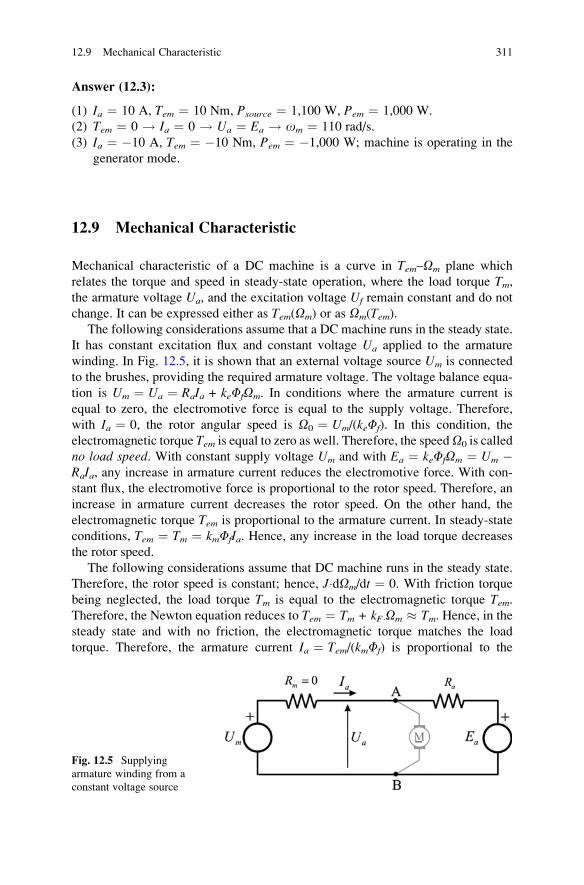
Answer (12.3):
(1) Ia ¼ 10 A, Tem ¼ 10 Nm, Psource ¼ 1,100 W, Pem ¼ 1,000 W.
(2) Tem ¼ 0 ! Ia ¼ 0 ! Ua ¼ Ea ! om ¼ 110 rad/s.
(3) Ia ¼ �10 A, Tem ¼ �10 Nm, Pem ¼ �1,000 W; machine is operating in the
generator mode.
12.9 Mechanical Characteristic
Mechanical characteristic of a DC machine is a curve in Tem–Om plane which
relates the torque and speed in steady-state operation, where the load torque Tm,the armature voltage Ua, and the excitation voltage Uf remain constant and do not
change. It can be expressed either as Tem(Om) or as Om(Tem).The following considerations assume that a DC machine runs in the steady state.
It has constant excitation flux and constant voltage Ua applied to the armature
winding. In Fig. 12.5, it is shown that an external voltage source Um is connected
to the brushes, providing the required armature voltage. The voltage balance equa-
tion is Um ¼ Ua ¼ RaIa + keFfOm. In conditions where the armature current is
equal to zero, the electromotive force is equal to the supply voltage. Therefore,
with Ia ¼ 0, the rotor angular speed is O0 ¼ Um/(keFf). In this condition, the
electromagnetic torque Tem is equal to zero as well. Therefore, the speedO0 is called
no load speed. With constant supply voltage Um and with Ea ¼ keFfOm ¼ Um �RaIa, any increase in armature current reduces the electromotive force. With con-
stant flux, the electromotive force is proportional to the rotor speed. Therefore, an
increase in armature current decreases the rotor speed. On the other hand, the
electromagnetic torque Tem is proportional to the armature current. In steady-state
conditions, Tem ¼ Tm ¼ kmFfIa. Hence, any increase in the load torque decreases
the rotor speed.
The following considerations assume that DC machine runs in the steady state.
Therefore, the rotor speed is constant; hence, J�dOm/dt ¼ 0. With friction torque
being neglected, the load torque Tm is equal to the electromagnetic torque Tem.Therefore, the Newton equation reduces to Tem ¼ Tm + kF�Om � Tm. Hence, in thesteady state and with no friction, the electromagnetic torque matches the load
torque. Therefore, the armature current Ia ¼ Tem/(kmFf) is proportional to the
Fig. 12.5 Supplying
armature winding from a
constant voltage source
12.9 Mechanical Characteristic 311
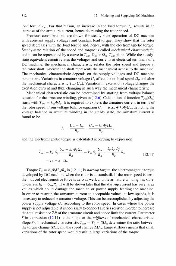
load torque Tm. For that reason, an increase in the load torque Tm results in an
increase of the armature current, hence decreasing the rotor speed.
Previous considerations are drawn for steady-state operation of DC machine
with constant supply voltages and constant load torque. They show that the rotor
speed decreases with the load torque and, hence, with the electromagnetic torque.
Steady-state relation of the speed and torque is called mechanical characteristic,and it can be represented by a curve in Tem–Om or Om–Tem plane. While the steady-
state equivalent circuit relates the voltages and currents at electrical terminals of a
DC machine, the mechanical characteristic relates the rotor speed and torque at
the rotor shaft, wherein the shaft represents the mechanical access to the machine.
The mechanical characteristic depends on the supply voltages and DC machine
parameters. Variations in armature voltage Ua affect the no load speed O0 and alter
the mechanical characteristic Tem(Om). Variation in excitation voltage changes the
excitation current and flux, changing in such way the mechanical characteristic.
Mechanical characteristic can be determined by starting from voltage balance
equation for the armature winding, given in (12.6). Calculation of function Tem(Om)
starts with Tem ¼ kmFfIa. It is required to express the armature current in terms of
the rotor speed. From voltage balance equation Ua ¼ RaIa + keFfOm, depicting the
voltage balance in armature winding in the steady state, the armature current is
found to be
Ia ¼ Um � Ea
Ra¼ Um � ke FfOm
Ra;
and the electromagnetic torque is calculated according to expression
Tem ¼ km FfUm � ke FfOm
Ra¼ km Ff
Um
Ra� kmke F2
f
RaOm
¼ T0 � S � Om:
(12.11)
Torque T0 ¼ kmFfUm/Ra in (12.11) is start-up torque, the electromagnetic torque
developed by DC machine when the rotor is at standstill. If the rotor speed is zero,
the induced electromotive force is zero as well, and the armature winding has start-up current I0 ¼ Um/Ra. It will be shown later that the start-up current has very large
values which could damage the machine or power supply feeding the machine.
In order to restrain the armature current to acceptable values, at low speeds, it is
necessary to reduce the armature voltage. This can be accomplished by adjusting the
power supply voltage Um according to the rotor speed. In cases where the power
supply is not adjustable, it is necessary to connect a series resistor in order to increase
the total resistance SR of the armature circuit and hence limit the current. Parameter
S in expression (12.11) is the slope or the stiffness of mechanical characteristic.
Slope S of mechanical characteristic Tem ¼ T0 � SOm determines the ratio between
the torque change DTem and the speed change DOm. Large stiffness means that small
variations of the rotor speed would result in large variations of the torque.
312 12 Modeling and Supplying DC Machines
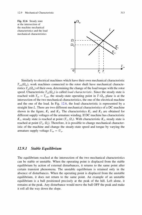
Similarly to electrical machines which have their own mechanical characteristic
Tem(Om), work machines connected to the rotor shaft have mechanical characte-
ristics Tm(Om) of their own, determining the change of the load torque with the rotor
speed. Characteristic Tm(Om) is called load characteristic. Since the steady state is
reached with Tm ¼ Tem, the steady-state operating point in T–Om plane is at the
intersection of the two mechanical characteristics, the one of the electrical machine
and the one of the load. In Fig. 12.6, the load characteristic is represented by a
straight line L. There are two different mechanical characteristics of a DC machine
shown in the figure, K1 and K2. The characteristics K1 and K2 are obtained for
different supply voltages of the armature winding. If DC machine has characteristic
K1, steady state is reached at point (T1, O1). With characteristic K2, steady state is
reached at point (T2, O2). Therefore, it is possible to change mechanical character-
istic of the machine and change the steady-state speed and torque by varying the
armature supply voltage Um ¼ Ua.
12.9.1 Stable Equilibrium
The equilibrium reached at the intersection of the two mechanical characteristics
can be stable or unstable. When the operating point is displaced from the stable
equilibrium by action of external disturbances, it returns to the same point after
certain transient phenomena. The unstable equilibrium is retained only in the
absence of disturbances. When the operating point is displaced from the unstable
equilibrium, it does not return to the same point. An example of an unstable
equilibrium is a ball positioned precisely at the peak of the hill. Left alone, it
remains at the peak. Any disturbance would move the ball OFF the peak and make
it roll all the way down the slope.
Fig. 12.6 Steady state
at the intersection of
the machine mechanical
characteristics and the load
mechanical characteristics
12.9 Mechanical Characteristic 313
Stability of the steady-state operating point depends on the stiffness of the two
mechanical characteristics. From the mechanical characteristic of DC machine
Tem ¼ T0 � SemOm and load characteristic Tm ¼ T0m � SmOm, it can be concluded
that the speed change DOm results in the electromagnetic torque change of
DTem ¼ �SemDOm and the load torque change of DTm ¼ �SmDOm. The influence
of parameters Sem and Sm on dynamic behavior of the system comprising one DC
machine and one work machine can be studied by starting from the steady-state
operating point where the DC machine runs at angular speed O1 and develops
electromagnetic torque T1, while the load machine resists to motion by the same
torque,Tm ¼ T1. In steady state, the speeddoesnot change, andNewton equation reads
JdOm
dt¼ Tem � Tm ¼ T1 � T1 ¼ 0:
The system is susceptible to external disturbances that may produce small
changes of the torque and speed. If a small variation of the rotor speed DOm occurs
for any reason, the rotor speed becomes O1 + DOm, while the electromagnetic
torque changes to T1 � SemDOm. At the same time, the load torque becomes
T1 � SmDOm. Since O1 is a constant, Newton equation becomes
Jd O1 þ DOmð Þ
dt¼ J
dDOm
dt¼ Tem � Tm
¼ T1 � SemDOm � T1 þ SmDOm
¼ Sm � Semð ÞDOm: (12.12)
With Sm � Sem > 0, a positive value of DOm gives a positive value of the first
derivative d(DOm)/dt. Therefore, disturbance DOm will progressively increase. A
negative disturbance DOm gives a negative value of the first derivative d(DOm)/dt.In this case, disturbance will progressively advance toward negative values of ever
larger magnitude. Hence, the steady-state operating point with Sm � Sem > 0 is
unstable. Namely, any disturbance, whatever the size and however small, puts the
system into instability.
With Sm � Sem < 0, a positive value of DOm gives a negative value of the first
derivative d(DOm)/dt. Therefore, disturbance DOm will decrease and gradually
converge toward zero, bringing the system to the original steady-state operating
point. This dynamic behavior is called stable since the system returns to the initial
steady state after being disturbed and moved from the equilibrium. On the other
hand, systems that progressively move away from the initial state and do not return
are called unstable.
Question (12.4): Starting from (12.12) and assuming that stiffness of the charac-
teristic and inertial torque are known, and that DOm(0) ¼ A, determine the change
DOm(t).
314 12 Modeling and Supplying DC Machines
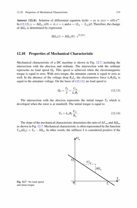
Answer (12.4): Solution of differential equation dy/dx ¼ ay is y(x) ¼ y(0)�eax.In (12.12), y ¼ DOm, y(0) ¼ A, x ¼ t, and а ¼ (Sm � Sem)/J. Therefore, the changeof DOm is determined by expression
DOmðtÞ ¼ DOmð0Þ � eSm�Sem
J t:
12.10 Properties of Mechanical Characteristic
Mechanical characteristic of a DC machine is shown in Fig. 12.7, including the
intersection with the abscissa and ordinate. The intersection with the ordinate
represents no load speed O0. This speed is achieved when the electromagnetic
torque is equal to zero. With zero torque, the armature current is equal to zero as
well. In the absence of the voltage drop RaIa, the electromotive force keFfOm is
equal to the armature voltage. On the basis of (12.11), no load speed is
O0 ¼ T0S
¼ Um
keFf: (12.13)
The intersection with the abscissa represents the initial torque T0 which is
developed when the rotor is at standstill. The initial torque is equal to
T0 ¼ kmFfUm
Ra: (12.14)
The slope of the mechanical characteristic determines the ratio ofDTem andDOm,
as shown in Fig. 12.7. Mechanical characteristic is often represented by the function
Tem(Om) ¼ T0 � SOm. In other words, the stiffness S is considered positive if the
Fig. 12.7 No load speed
and nitial torque
12.10 Properties of Mechanical Characteristic 315
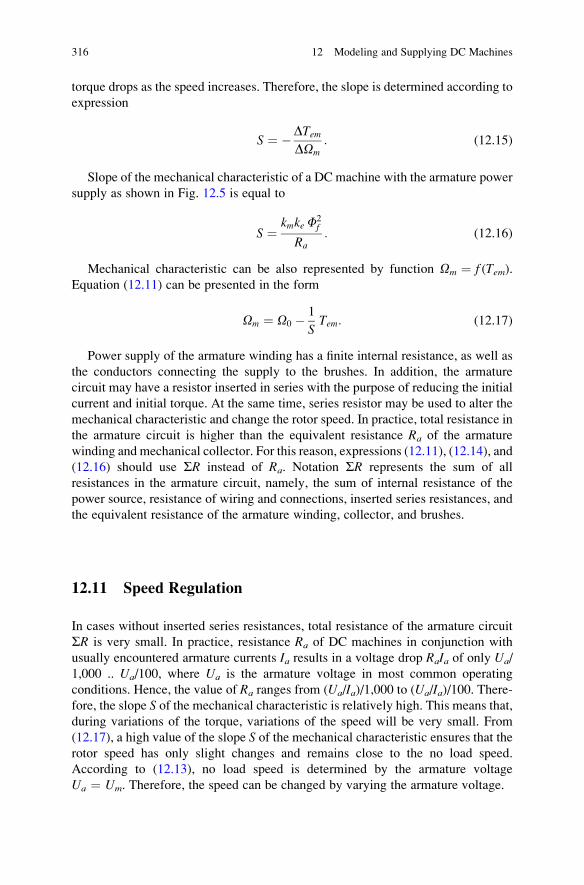
torque drops as the speed increases. Therefore, the slope is determined according to
expression
S ¼ �DTemDOm
: (12.15)
Slope of the mechanical characteristic of a DC machine with the armature power
supply as shown in Fig. 12.5 is equal to
S ¼ kmke F2f
Ra: (12.16)
Mechanical characteristic can be also represented by function Om ¼ f (Tem).Equation (12.11) can be presented in the form
Om ¼ O0 � 1
STem: (12.17)
Power supply of the armature winding has a finite internal resistance, as well as
the conductors connecting the supply to the brushes. In addition, the armature
circuit may have a resistor inserted in series with the purpose of reducing the initial
current and initial torque. At the same time, series resistor may be used to alter the
mechanical characteristic and change the rotor speed. In practice, total resistance in
the armature circuit is higher than the equivalent resistance Ra of the armature
winding and mechanical collector. For this reason, expressions (12.11), (12.14), and
(12.16) should use SR instead of Ra. Notation SR represents the sum of all
resistances in the armature circuit, namely, the sum of internal resistance of the
power source, resistance of wiring and connections, inserted series resistances, and
the equivalent resistance of the armature winding, collector, and brushes.
12.11 Speed Regulation
In cases without inserted series resistances, total resistance of the armature circuit
SR is very small. In practice, resistance Ra of DC machines in conjunction with
usually encountered armature currents Ia results in a voltage drop RaIa of only Ua/
1,000 .. Ua/100, where Ua is the armature voltage in most common operating
conditions. Hence, the value of Ra ranges from (Ua/Ia)/1,000 to (Ua/Ia)/100. There-fore, the slope S of the mechanical characteristic is relatively high. This means that,
during variations of the torque, variations of the speed will be very small. From
(12.17), a high value of the slope S of the mechanical characteristic ensures that the
rotor speed has only slight changes and remains close to the no load speed.
According to (12.13), no load speed is determined by the armature voltage
Ua ¼ Um. Therefore, the speed can be changed by varying the armature voltage.
316 12 Modeling and Supplying DC Machines
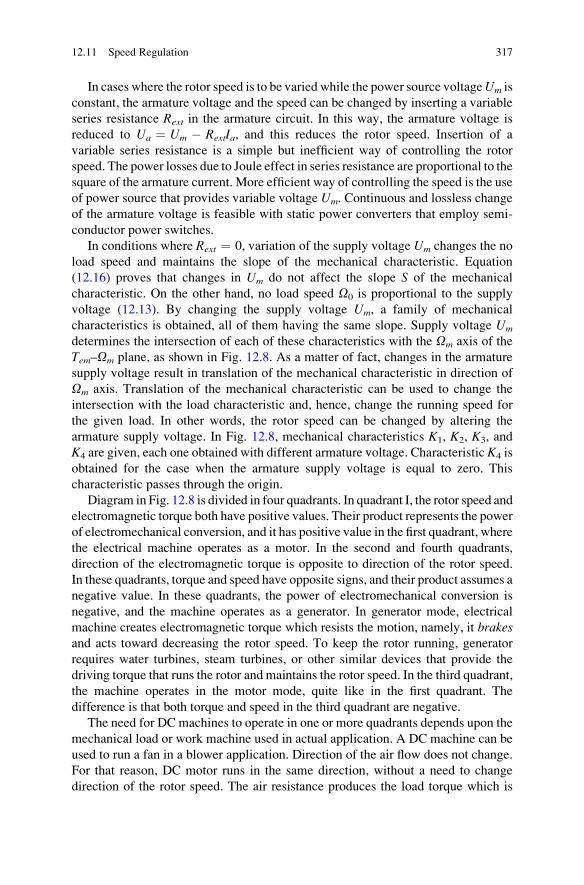
In cases where the rotor speed is to be varied while the power source voltageUm is
constant, the armature voltage and the speed can be changed by inserting a variable
series resistance Rext in the armature circuit. In this way, the armature voltage is
reduced to Ua ¼ Um � RextIa, and this reduces the rotor speed. Insertion of a
variable series resistance is a simple but inefficient way of controlling the rotor
speed. The power losses due to Joule effect in series resistance are proportional to the
square of the armature current. More efficient way of controlling the speed is the use
of power source that provides variable voltage Um. Continuous and lossless change
of the armature voltage is feasible with static power converters that employ semi-
conductor power switches.
In conditions where Rext ¼ 0, variation of the supply voltage Um changes the no
load speed and maintains the slope of the mechanical characteristic. Equation
(12.16) proves that changes in Um do not affect the slope S of the mechanical
characteristic. On the other hand, no load speed O0 is proportional to the supply
voltage (12.13). By changing the supply voltage Um, a family of mechanical
characteristics is obtained, all of them having the same slope. Supply voltage Um
determines the intersection of each of these characteristics with the Om axis of the
Tem–Om plane, as shown in Fig. 12.8. As a matter of fact, changes in the armature
supply voltage result in translation of the mechanical characteristic in direction of
Om axis. Translation of the mechanical characteristic can be used to change the
intersection with the load characteristic and, hence, change the running speed for
the given load. In other words, the rotor speed can be changed by altering the
armature supply voltage. In Fig. 12.8, mechanical characteristics K1, K2, K3, and
K4 are given, each one obtained with different armature voltage. Characteristic K4 is
obtained for the case when the armature supply voltage is equal to zero. This
characteristic passes through the origin.
Diagram in Fig. 12.8 is divided in four quadrants. In quadrant I, the rotor speed and
electromagnetic torque both have positive values. Their product represents the power
of electromechanical conversion, and it has positive value in the first quadrant, where
the electrical machine operates as a motor. In the second and fourth quadrants,
direction of the electromagnetic torque is opposite to direction of the rotor speed.
In these quadrants, torque and speed have opposite signs, and their product assumes a
negative value. In these quadrants, the power of electromechanical conversion is
negative, and the machine operates as a generator. In generator mode, electrical
machine creates electromagnetic torque which resists the motion, namely, it brakesand acts toward decreasing the rotor speed. To keep the rotor running, generator
requires water turbines, steam turbines, or other similar devices that provide the
driving torque that runs the rotor and maintains the rotor speed. In the third quadrant,
the machine operates in the motor mode, quite like in the first quadrant. The
difference is that both torque and speed in the third quadrant are negative.
The need for DC machines to operate in one or more quadrants depends upon the
mechanical load or work machine used in actual application. A DC machine can be
used to run a fan in a blower application. Direction of the air flow does not change.
For that reason, DC motor runs in the same direction, without a need to change
direction of the rotor speed. The air resistance produces the load torque which is
12.11 Speed Regulation 317
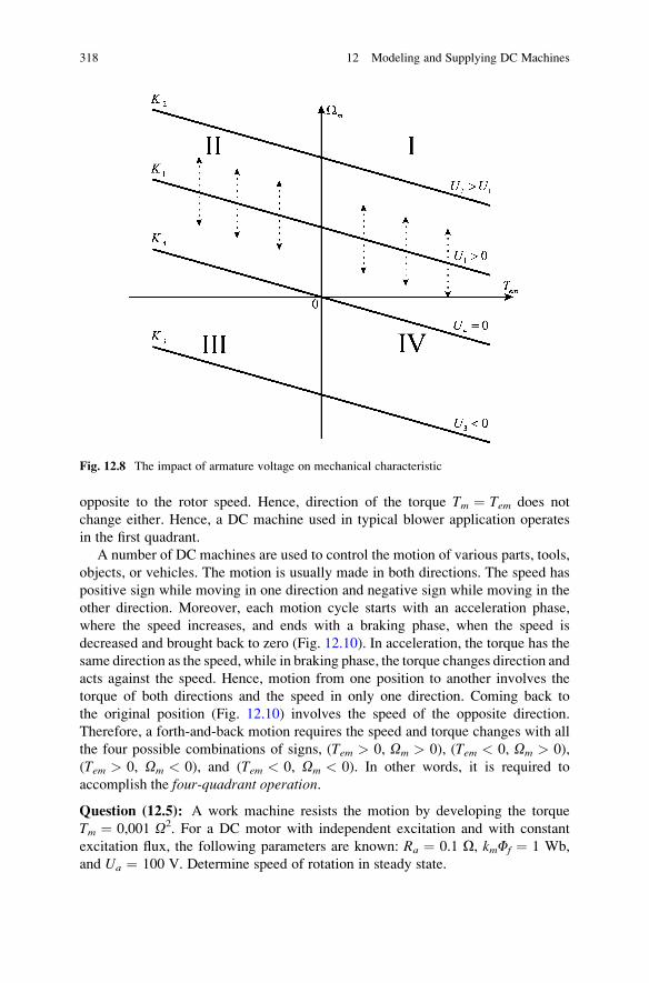
opposite to the rotor speed. Hence, direction of the torque Tm ¼ Tem does not
change either. Hence, a DC machine used in typical blower application operates
in the first quadrant.
A number of DC machines are used to control the motion of various parts, tools,
objects, or vehicles. The motion is usually made in both directions. The speed has
positive sign while moving in one direction and negative sign while moving in the
other direction. Moreover, each motion cycle starts with an acceleration phase,
where the speed increases, and ends with a braking phase, when the speed is
decreased and brought back to zero (Fig. 12.10). In acceleration, the torque has the
same direction as the speed, while in braking phase, the torque changes direction and
acts against the speed. Hence, motion from one position to another involves the
torque of both directions and the speed in only one direction. Coming back to
the original position (Fig. 12.10) involves the speed of the opposite direction.
Therefore, a forth-and-back motion requires the speed and torque changes with all
the four possible combinations of signs, (Tem > 0, Om > 0), (Tem < 0, Om > 0),
(Tem > 0, Om < 0), and (Tem < 0, Om < 0). In other words, it is required to
accomplish the four-quadrant operation.
Question (12.5): A work machine resists the motion by developing the torque
Tm ¼ 0,001 O2. For a DC motor with independent excitation and with constant
excitation flux, the following parameters are known: Ra ¼ 0.1 O, kmFf ¼ 1 Wb,
and Ua ¼ 100 V. Determine speed of rotation in steady state.
Fig. 12.8 The impact of armature voltage on mechanical characteristic
318 12 Modeling and Supplying DC Machines
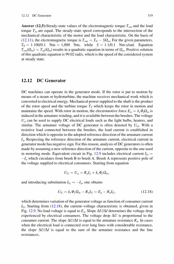
Answer (12.5):Steady-state values of the electromagnetic torque Tem and the load
torque Tm are equal. The steady-state speed corresponds to the intersection of the
mechanical characteristic of the motor and the load characteristic. On the basis of
(12.11), the electromagnetic torque is Tem ¼ T0 � SOm. For the given parameters,
T0 ¼ 1�100/0.1 Nm ¼ 1,000 Nm, while S ¼ 1�1/0.1 Nm�s/rad. Equation
Tem(Om) ¼ Tm(Om) results in a quadratic equation in terms of Om. Positive solution
of this quadratic equation is 99.02 rad/s, which is the speed of the considered system
at steady state.
12.12 DC Generator
DC machines can operate in the generator mode. If the rotor is put to motion by
means of a steam or hydroturbine, the machine receives mechanical work which is
converted to electrical energy. Mechanical power supplied to the shaft is the product
of the rotor speed and the turbine torque TT which keeps the rotor in motion and
maintains the speed. With rotor in motion, the electromotive force Ea ¼ keFfOm is
induced in the armature winding, and it is available between the brushes. The voltage
Ua can be used to supply DC electrical loads such as the light bulbs, heaters, and
similar. The armature voltage of DC generator is often denoted by UG. With a
resistive load connected between the brushes, the load current is established in
direction which is opposite to the adopted reference direction of the armature current
Ia. Respecting the reference direction of the armature current, electrical current in
generator mode has negative sign. For this reason, analysis of DC generators is often
made by assuming a new reference direction of the current, opposite to the one used
in motoring mode. Equivalent circuit in Fig. 12.9 includes electrical current IG ¼�Ia which circulates from brush B to brush A. Brush A represents positive pole of
the voltage supplied to electrical consumers. Starting from equation
UG ¼ Ua ¼ RaIa þ keFfOm;
and introducing substitution IG ¼ �Ia, one obtains
UG ¼ keFfOm � RaIG ¼ Ea � RaIG; (12.18)
which determines variation of the generator voltage as function of consumer current
IG. Starting from (12.18), the current–voltage characteristic is obtained, given in
Fig. 12.9. No load voltage is equal to Ea. Slope DU/DI determines the voltage drop
experienced by electrical consumers. The voltage drop DU is proportional to the
consumer current. The slope DU/DI is equal to the armature resistance Ra. In cases
when the electrical load is connected over long lines with considerable resistance,
the slope DU/DI is equal to the sum of the armature resistance and the line
resistances.
12.12 DC Generator 319
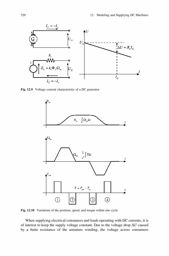
When supplying electrical consumers and loads operating with DC currents, it is
of interest to keep the supply voltage constant. Due to the voltage drop DU caused
by a finite resistance of the armature winding, the voltage across consumers
Fig. 12.9 Voltage–current characteristic of a DC generator
Fig. 12.10 Variations of the position, speed, and torque within one cycle
320 12 Modeling and Supplying DC Machines
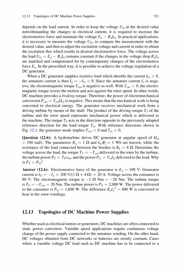
depends on the load current. In order to keep the voltage UG at the desired value
notwithstanding the changes in electrical current, it is required to increase the
electromotive force and maintain the voltage Ea � RaIG. In practical applications,
it is necessary to measure the voltage UG, to compare the measurement with the
desired value, and then to adjust the excitation voltage and current in order to obtain
the excitation flux which results in desired electromotive force. The voltage across
the load UG ¼ Ea � RaIG remains constant if the changes in the voltage drop RaIGare matched and compensated for by contemporary changes of the electromotive
force Ea. In the prescribed way, it is possible to achieve the voltage regulation of a
DC generator.
When a DC generator supplies resistive load which absorbs the current IG > 0,
the armature current is then Ia ¼ �IG < 0. Since the armature current Ia is nega-tive, the electromagnetic torque Tem is negative as well. With Tem < 0, the electro-
magnetic torque resists the motion and acts against the rotor speed. In other words,
DC machine provides a braking torque. Therefore, the power of electromechanical
conversion Pem ¼ TemOm is negative. This means that the mechanical work is being
converted to electrical energy. The generator receives mechanical work from a
driving turbine by means of the shaft. The product of the driving torque TT of theturbine and the rotor speed represents mechanical power which is delivered to
the machine. The torque TT acts in the direction opposite to the previously adopted
reference direction for the load torque Tm. With reference directions shown in
Fig. 12.1, the generator mode implies Tem < 0 and Tm < 0.
Question (12.6): A hydroturbine drives DC generator at angular speed of Om
¼ 100 rad/s. The parameters Ra ¼ 1 O and kmFf ¼ 1 Wb are known, while the
resistance of the load connected between the brushes is RL ¼ 4 O. Determine the
voltage across the load, the torque TT ¼ �Tem delivered to the rotor by the turbine,
the turbine power PT ¼ TTom, and the power PG ¼ UaIG delivered to the load.Why
is PT > PG?
Answer (12.6): Electromotive force of the generator is Ea ¼ 100 V. Generator
current is IG ¼ �Ia ¼ 100 V/(1 O + 4 O) ¼ 20 A. Voltage across the consumer is
80 V. The electromagnetic torque is �1�20 Nm ¼ �20 Nm. The turbine torque
is TT ¼ �Tem ¼ 20 Nm. The turbine power is PT ¼ 2,000 W. The power delivered
to the consumer is PG ¼ 1,600 W. The difference RaIa2 ¼ 400 W is converted to
heat in the rotor windings.
12.13 Topologies of DC Machine Power Supplies
Whether used as electrical motors or generators, DCmachines are often connected to
static power converters. Variable speed applications require continuous voltage
change of the power supply connected to the armature winding. On the other hand,
DC voltages obtained from DC networks or batteries are mostly constant. Cases
where a variable voltage DC load such as DC machine has to be connected to a
12.13 Topologies of DC Machine Power Supplies 321
constant voltage source are frequently encountered. In such cases, it is necessary to
use aDC/DC static power converter which conditions the armature voltage according
to needs.Moreover, DCmachines are often supplied fromACmains. In these cases, it
is necessary to use static power converter which converts constant AC voltages in
adjustable DC voltage. Most common topologies of static power converters used
in conjunction with DC machines are discussed in the following section.
12.13.1 Armature Power Supply Requirements
A DC motor takes electrical energy from power source, performs electromechani-
cal conversion, and delivers mechanical work to the output shaft. Electrical motors
are usually cylindrical rotating machines which deliver the driving torque to work
machines by means of the rotor shaft and subsequent mechanical couplings.
Mechanical power delivered to work machine is determined by the product of the
driving torque and the speed of rotation.
It is of interest to specify the required characteristics of the power source supply-
ing the armature winding. A DC motor is mainly used for controlling the motion of
tools, workpieces, semifinished articles, finished articles, packaging machines,
manipulators, vehicles, and other objects. A typical motion cycle includes start
from initial position, motion toward the targeted position, reaching the target and
resting at the target position, and then turning back to the initial position. Represen-
tative motion cycle is depicted in Fig. 12.10 by typical changes in the position ym,speed Om, and torque Tem in the course of moving from the start position to the target
and coming back. In order to get a closer specification for the armature power supply,
it is of interest to observe the torque and speed changes during this motion.
Characteristic phases of the motion cycle are denoted by numbers 1 to 4. In
phase 1, the torque has positive value, and it accelerates the motor, increasing the
speed and initiating the motion toward target position. It is observed in Fig. 12.10
that the desired speed is reached soon and then the torque reduces while the speed
remains constant. In constant speed interval between the phases 1 and 2, the torque
is very low. With constant speed and with no need to provide the acceleration
torque JdOm/dt, the torque reduces to a very small friction, and it is considered as
equal to zero. In phase 2, position ym gets close to the target position. For this
reason, it is necessary to brake and reduce the speed. Negative torque is developed
in order to reduce the speed to zero and eventually stop at the target position. In the
course of coming back to the initial position, the speed and torque required in
phases 3 and 4 are of the opposite direction compared to the speed and torque
required in phases 1 and 2. It can be concluded that the motion cycle given in
Fig. 12.10 comprises the following four combinations of the speed and torque
directions:
• Tem > 0, Om > 0 (phase 1)
• Tem < 0, Om > 0 (phase 2)
322 12 Modeling and Supplying DC Machines
• Tem < 0, Om < 0 (phase 3)
• Tem > 0, Om < 0 (phase 4)
In the first and third phases, the electrical machine operates in motor mode,
while in the second and fourth phases, it operates in generator mode. Hence,
throughout the motion cycle depicted in Fig. 12.10, the operating point (Tem–Om)
has to pass through all the four quadrants of the torque-speed plane. This can be
used to specify the armature power supply and define the required voltages and
currents. The torque Tem ¼ kmFf Ia is determined by the armature current. Direc-
tion of the electromagnetic torque is determined by the sign of the armature
current Ia. At the same time, the voltage drop RaIa is often neglected, and the
armature voltage Ua is assumed to be close to the induced electromotive force
Ea ¼ keFfOm. Therefore, the sign of the voltage Ua is determined by direction of
the rotor speed. With Ua � keFfOm and Ia ¼ Tem/(kmFf), the change of the
operating point in Tem–Om plane can be used to envisage the required voltages
and currents in (Ia � Ua) plane. In this way, it is possible to specify the
characteristics of the power source intended for supplying the armature winding.
From the previous conclusions and from relations Tem ¼ kmFf Ia and Ua � Ea ¼keFfOm, it can be concluded that, in the course of motion cycle depicted in
Fig. 12.10, the voltage and current of the armature winding change signs in the
following way:
• Ia > 0, Ua > 0 (phase 1)
• Ia < 0, Ua > 0 (phase 2)
• Ia < 0, Ua < 0 (phase 3)
• Ia > 0, Ua < 0 (phase 4)
Therefore, the power source for supplying the armature winding should provide
voltages and currents of both directions and in all the four combinations. These
requirements are crucial for the topology of the static power converter intended for
supplying the DC machine.
There are applications of DC motors where the speed and torque do not change
the sign. In these cases, the power source supplying the armature winding is more
simple. In earlier mentioned example of a fan driver, the machine operates in the
first quadrant, and armature winding can be supplied by a static power converter
with strictly positive voltages and currents, Ia > 0 and Ua > 0.
12.13.2 Four Quadrants in T–V and U–I Diagrams
If a DC machine is used to effectuate the motion shown in Fig. 12.10, in different
phases of this motion, it passes through all the four quadrants of the T–O plane.
If direction of the excitation flux does not change, direction of the torque is
determined by direction of the armature current, while direction of the electro-
motive force is determined by direction of the angular rotor speed. Applying the
12.13 Topologies of DC Machine Power Supplies 323
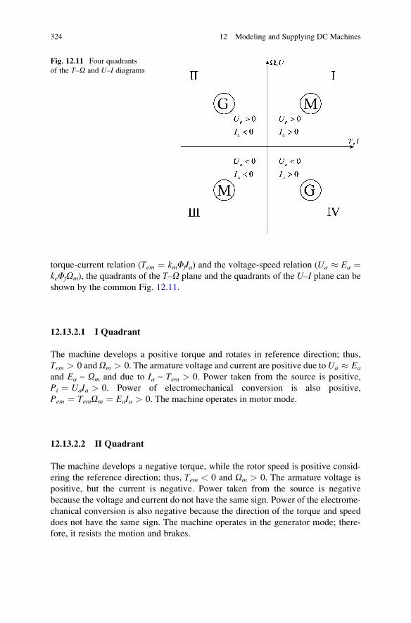
torque-current relation (Tem ¼ kmFfIa) and the voltage-speed relation (Ua � Ea ¼keFfOm), the quadrants of the T–O plane and the quadrants of the U–I plane can be
shown by the common Fig. 12.11.
12.13.2.1 I Quadrant
The machine develops a positive torque and rotates in reference direction; thus,
Tem > 0 andOm > 0. The armature voltage and current are positive due toUa � Ea
and Ea ~ Om and due to Ia ~ Tem > 0. Power taken from the source is positive,
Pi ¼ UaIa > 0. Power of electromechanical conversion is also positive,
Pem ¼ TemOm ¼ EaIa > 0. The machine operates in motor mode.
12.13.2.2 II Quadrant
The machine develops a negative torque, while the rotor speed is positive consid-
ering the reference direction; thus, Tem < 0 and Om > 0. The armature voltage is
positive, but the current is negative. Power taken from the source is negative
because the voltage and current do not have the same sign. Power of the electrome-
chanical conversion is also negative because the direction of the torque and speed
does not have the same sign. The machine operates in the generator mode; there-
fore, it resists the motion and brakes.
Fig. 12.11 Four quadrants
of the T–O and U–I diagrams
324 12 Modeling and Supplying DC Machines
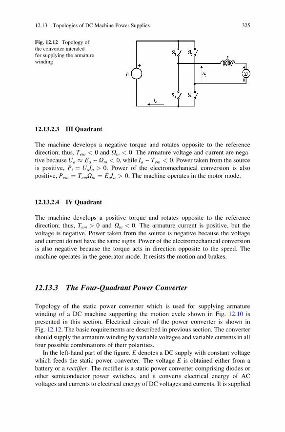
12.13.2.3 III Quadrant
The machine develops a negative torque and rotates opposite to the reference
direction; thus, Tem < 0 and Om < 0. The armature voltage and current are nega-
tive because Ua � Ea ~ Om < 0, while Ia ~ Tem < 0. Power taken from the source
is positive, Pi ¼ UaIa > 0. Power of the electromechanical conversion is also
positive, Pem ¼ TemOm ¼ EaIa > 0. The machine operates in the motor mode.
12.13.2.4 IV Quadrant
The machine develops a positive torque and rotates opposite to the reference
direction; thus, Tem > 0 and Om < 0. The armature current is positive, but the
voltage is negative. Power taken from the source is negative because the voltage
and current do not have the same signs. Power of the electromechanical conversion
is also negative because the torque acts in direction opposite to the speed. The
machine operates in the generator mode. It resists the motion and brakes.
12.13.3 The Four-Quadrant Power Converter
Topology of the static power converter which is used for supplying armature
winding of a DC machine supporting the motion cycle shown in Fig. 12.10 is
presented in this section. Electrical circuit of the power converter is shown in
Fig. 12.12. The basic requirements are described in previous section. The converter
should supply the armature winding by variable voltages and variable currents in all
four possible combinations of their polarities.
In the left-hand part of the figure, E denotes a DC supply with constant voltage
which feeds the static power converter. The voltage E is obtained either from a
battery or a rectifier. The rectifier is a static power converter comprising diodes or
other semiconductor power switches, and it converts electrical energy of AC
voltages and currents to electrical energy of DC voltages and currents. It is supplied
Fig. 12.12 Topology of
the converter intended
for supplying the armature
winding
12.13 Topologies of DC Machine Power Supplies 325
either from a single-phase or from a three-phase network. At the input of a rectifier,
there are AC voltages and currents. Mains-supplied rectifier has the AC quantities
at the line frequency (50 or 60 Hz). The rectifier performs AC/DC conversion and
feeds the electrical energy in the form of DC voltages and currents. A diode rectifier
provides the output DC voltage E which is proportional to the rms value of the AC
voltages across the input terminals. Therefore, mains-supplied diode rectifiers
cannot provide variable DC voltage E.Receiving the energy from the DC supply E, it is necessary to perform the
conversion and provide variable armature voltage of both polarities, positive and
negative. Solution which satisfies the needs is the bridge comprising four switches,
S1, S2, S3, and S4. Within these preliminary considerations, the switches are
considered to be ideal. This means that they do not carry any electrical current
when turned OFF (open). At the same time, the voltage drop across the switch
which is turned ON (closed) is considered negligible and equal to zero. This means
that any switch in the state of conduction (closed) does not have any conductionlosses. Moreover, it is also assumed that the processes of closing and opening
the switch do not involve any losses. Hence, there are no commutation losses. Thetransients of changing the switch state are called commutation.
12.13.3.1 Power Switches
Real mechanical switches as well as semiconductor power switches carry a small
amount of leakage current even when switched OFF. Besides, in their state of
conduction (ON, closed), they have a small voltage drop across the switch. Hence,
real switches do have a certain amount of conduction losses. Each process of
turning ON or OFF a semiconductor power switch and each process of closing or
opening a mechanical switch involve energy losses. The energy loss incurred in
each commutation is multiplied by the number of commutations per second to
obtain the commutation losses.
Mechanical switches have contacts which close (get in touch) or open (get
detached) in order to operate the switch. Turn-OFF commutation losses in mechan-
ical switches arise due to an intermittent electrical arc which appears during
separation of contacts. Even though the contacts are being detached, the current
continues for a short while through an electric arc which breaks up in the space
between contacts. The contacts are disengaged quickly, and the arc is very brief.
Yet, it contributes to energy losses. Turn-ON commutation losses of mechanical
switches arise due to electrical current being established prior to proper closing of
the contacts, which contributes to the commutation losses.
Contemporary static power converters feeding the armature winding do not use
mechanical switches. Instead, semiconductor power switches are used, such as BJT
(bipolar junction transistors), MOSFET (metal oxide field effect transistors), and
IGBT (insulated gate bipolar transistors). In semiconductor power switches, com-
mutation losses arise due to phenomena of a different nature. Due to transient
processes within semiconductor power switches, the change from the OFF state,
326 12 Modeling and Supplying DC Machines
characterized by u ¼ E and i � 0, into the ON state, characterized by u � 0 and
i ¼ Ia, a brief commutation interval Dtc exists where considerable voltage and
considerable current exist at the same time. Commutation time Dtc is different forBJT, MOSFET, and IGBT transistors, and it ranges from 100 ns up to 1 ms. The time
integral of the ui product during the commutation interval represents the energy loss
incurred during one commutation event. In both cases of mechanical and semicon-
ductor switches, power of commutation losses is dependent on the energy loss of
single commutation and on the number of commutations per second.
By closing switches S1 and S4, the voltage +E is established between brushes A
and B. By closing switches S2 and S3, the voltage�E is established between brushes
A and B. Therefore, the switching bridge shown in Fig. 12.12 provides voltages of
both polarities. Current through the closed switches is equal to the armature current.
As the armature current has both directions, the switches should be capable of
conducting the current in both directions. According to previous considerations, the
voltage and current direction depend on the quadrant where the operating point of
the machine resides.
12.13.3.2 Switching States
Each of the four switches is closed (ON) or opened (OFF). Assuming that all the
switches can be controlled independently, the number of switching states for
the four switches is 24 ¼ 16. When the switches are connected to the switching
bridge, shown in Fig. 12.12, the number of available switching states is reduced.
Considering switches S1 and S2, the switching state S1 ¼ S2 ¼ ON would bring
the power sourceE into short circuit. At the same time, the switching state S1 ¼ S2 ¼OFF would leave no path for the armature current and cannot be used either. Hence,
the branch (arm) S1–S2 has only two available switching states, and these are
(S1 ¼ ON, S2 ¼ OFF) and (S1 ¼ OFF, S2 ¼ ON). The same holds for branch
S3–S4. With two branches (arms) and with two possible switching states in each
branch, the number of distinct switching states for the entire switching bridge is four.
The same conclusion regarding the number of possible switching states can be
obtained by reasoning whether the number of switches being turned ON at any
given instant should be 0, 1, 2, 3, or 4. Considering the switching bridge in
Fig. 12.12, it has to be noted that the number of switches is turned ON 2 at each
instant. First of all, it can be neither 4 nor 3. If the number of turned-ON switches is
3, then either the branch S1–S2 or the branch S3–S4 would bring the source E into
short circuit. The source E is either a battery or a diode rectifier, and it has a very
small internal resistance. Therefore, turning ON of one entire branch would lead to
very high current through the source and through the switches, leading very quickly
to their permanent damage. On the other hand, the number of turned-ON switches
cannot be less than 2. This is due to the fact that the switching bridge must provide
the path for the armature current at any instant, due to the fact that the armature
current cannot be interrupted. The armature current gets from the branch S1–S2 tothe brush A and then from the brush B to the branch S3–S4. For the purpose of
12.13 Topologies of DC Machine Power Supplies 327
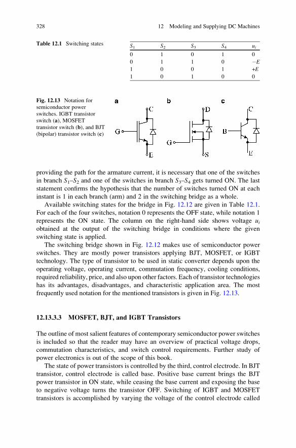
providing the path for the armature current, it is necessary that one of the switches
in branch S1–S2 and one of the switches in branch S3–S4 gets turned ON. The last
statement confirms the hypothesis that the number of switches turned ON at each
instant is 1 in each branch (arm) and 2 in the switching bridge as a whole.
Available switching states for the bridge in Fig. 12.12 are given in Table 12.1.
For each of the four switches, notation 0 represents the OFF state, while notation 1
represents the ON state. The column on the right-hand side shows voltage uiobtained at the output of the switching bridge in conditions where the given
switching state is applied.
The switching bridge shown in Fig. 12.12 makes use of semiconductor power
switches. They are mostly power transistors applying BJT, MOSFET, or IGBT
technology. The type of transistor to be used in static converter depends upon the
operating voltage, operating current, commutation frequency, cooling conditions,
required reliability, price, and also upon other factors. Each of transistor technologies
has its advantages, disadvantages, and characteristic application area. The most
frequently used notation for the mentioned transistors is given in Fig. 12.13.
12.13.3.3 MOSFET, BJT, and IGBT Transistors
The outline of most salient features of contemporary semiconductor power switches
is included so that the reader may have an overview of practical voltage drops,
commutation characteristics, and switch control requirements. Further study of
power electronics is out of the scope of this book.
The state of power transistors is controlled by the third, control electrode. In BJT
transistor, control electrode is called base. Positive base current brings the BJT
power transistor in ON state, while ceasing the base current and exposing the base
to negative voltage turns the transistor OFF. Switching of IGBT and MOSFET
transistors is accomplished by varying the voltage of the control electrode called
Table 12.1 Switching states S1 S2 S3 S4 ui
0 1 0 1 0
0 1 1 0 �E
1 0 0 1 +E
1 0 1 0 0
Fig. 12.13 Notation for
semiconductor power
switches. IGBT transistor
switch (a), MOSFET
transistor switch (b), and BJT
(bipolar) transistor switch (c)
328 12 Modeling and Supplying DC Machines
gates. The gate voltage of +15 V is larger than the threshold VT ∈ [+4 V .. +6 V],
and it brings the transistor into conduction state (ON). Turning OFF is achieved by
applying�15 V to the gate. Supplying the base current to large BJT transistors may
involve considerable amount of power, while the gate control of IGBT and
MOSFET transistors is virtually lossless.
All the three families of power transistors have very small currents while in OFF
state. Their ON behavior is different. The voltage drop across power transistor in the
state of conduction (ON) is rather small. Roughly, it varies between 100mV and 3V.
Bipolar junction transistor (BJT) is turned ON by feeding the base which is suffi-
ciently high current to bring the transistor to the state of saturation, when the voltageVCE ¼ VBE � VBC across collector and emitter terminals is very small. Small BJT
transistors in the state of saturation may have VCE as low as 200 mV. Power BJT
transistors have their internal voltage drops and may have the values of VCE
anywhere between 500mV and 1V. On the other hand, large-current BJT transistors
have relatively low current gain b ¼ IC/IB and require very large base current. For
that reason, most semiconductor power switches in BJT technology have two
transistors connected in Darlington configuration where the voltage drop in ON
state is VCE ¼ 2VBE � VBC, ranging between 1.5 and 3 V.
The MOSFET and IGBT transistors are turned ON by applying +15 V to the
gate. MOSFET transistors in ON state behave as a resistor and have voltage drop of
RONIDS, where RON is the “ON” of the MOSFET channel. Transistors made for
operating voltages below 100 V may have RON of only 1 mO, resulting in very low
voltage drops. Therefore, these transistors are preferred choice for all applications
with low operating voltages. Due to specific properties of power MOSFET
switches, their resistance RON increases with the maximum sustainable voltages.
Due to RON ~ U2.5, transistor made to sustain twice the voltage would have 5.6 time
larger resistance in ON state. For that reason, high-voltage MOSFET transistors are
rarely used due to their large voltage drop. IGBT power transistors are developed as
a hybrid of BJT and MOSFET technologies, combining positive characteristics of
the both. Therefore, they are widely used and made available for voltages up to
several kilovolts and currents above 1 kA.
12.13.3.4 Freewheeling Diodes
Electrical current in armature winding changes direction to provide both motoring
and braking torques. Therefore, each of the switches has to be ready to conduct
electrical currents in both directions. Power switches in Fig. 12.13 are mostly made
with power transistors. Placing one power transistor in place of the switches S1, S2,S3, and S4 is not sufficient since power transistors operate with only one direction ofcurrent. When turned ON, bipolar transistor conducts the current that enters collec-
tor and goes to emitter. An attempt to establish emitter current of opposite direction
is of little use. Power transistors are suited for bidirectional currents. Any inverse
current may result in significant losses and eventually damage semiconductor
device. Therefore, the use of transistors with inverse current is not of interest in
12.13 Topologies of DC Machine Power Supplies 329
static power converters. Transistors such as BJT, IGBT, and MOSFET are used to
conduct electrical current only in one direction. For this reason, each of the switches
S1.. S4 has one power transistor and one semiconductor power diode. Element
denoted by (C) in Fig. 12.13 is a parallel connection of one bipolar transistor
conducting in CE direction and one power diode conducting in EC direction. All
the four switches shown in Fig. 12.12 are constructed in the prescribed way.
Therefore, each of S1.. S4 switches should be considered as a parallel connection
of one power transistor and one power diode.
12.13.3.5 Available Output Voltages
According to Table 12.1, a positive voltage across the armature winding is obtained
by turning ON the switches S1 and S4. In this switching state, positive armature
current circulates through power transistors within switches S1 and S4. Otherwise,with negative armature current, the current is established through power diodes
within switches S1 and S4, connected in parallel with power transistors. Negative
voltage across the armature winding is obtained by turning ON the switches S2 andS3. The same way as the previous, this switching state can be used for armature
currents in both directions. There are also the switching states S1 ¼ S3 ¼ ON and
S2 ¼ S4 ¼ ON which provide the armature voltage ui ¼ 0.
The switching structure in Fig. 12.12 with four available switching states allows
feeding the armature winding by voltages and currents of both polarities. Therefore,
it is compatible with the need to operate DC machine in all the four quadrants in
Tem–Om plane. Prescribed method cannot provide continuous change in armature
voltage. Namely, there are only four available switching states, and they provide the
output voltages of +E, �E, or 0. Hence, the armature winding can be supplied by
the voltage that assumes one of the three discrete values. Instantaneous value of
the armature voltage cannot have a continuous change. On the other hand, the
armature voltage can be supplied by the train of pulses. The change (modulation) of
the pulse-width changes the average value of the armature voltage.
Question (12.7): What are the switching states that provide armature voltage equal
to zero?
Answer (12.7): By turning ON switches S2 and S4, armature voltage is made equal
to zero. Armature winding is short circuited also when switches S1 and S3 are
switched ON.
12.13.4 Pulse-Width Modulation
According to analysis summarized in Table 12.1, the output voltage ui may have
one of the three available values, +E, �E, or 0. It has been shown that application
of DC electrical motors requires continuous variation of the supply voltage.
330 12 Modeling and Supplying DC Machines
The switching structure in Fig. 12.12 cannot produce continuous change of the
output voltage. On the other hand, it is possible to devise a sequence of switching
states that would repeat in relatively short periods called switching periods. Eachswitching state may have adjustable duration and provide the armature voltages +E,�E, or 0. Sequential repetition of discrete voltages +E,�E, and/or 0 would result inan average voltage +E > Uav > �E. The voltage ui would assume the form of a
train of pulses of variable width. The width of the pulses would affect the average
voltage Uav within each switching period. It is obvious, though, that variation of
pulse width cannot result in continuous change of the instantaneous voltage. It is
possible to change only the average value of the armature voltage within each
switching period. Variation of pulse width is called pulse-width modulation.
12.13.4.1 Armature Voltage Requirements
In the areas of industrial robots, electrical vehicles, and in majority of applications
involving motion control, there is a need for continuous variation of the speed of
electrical motors. The steady-state armature voltage is equal to Ua ¼ RaIa þkeFfOm. The voltage drop RaIa is usually much lower than the electromotive
force. Windings of electrical machines are made to have small resistance, so as to
reduce losses due to Joule effect and increase the efficiency. Therefore, it is justified
to assume that Ua � keFfOm. With constant flux, the armature voltage is propor-
tional to the rotor speed. As the speed changes continuously, the voltage must have
continuous changes as well. The available voltage sources are usually batteries or
diode rectifiers with constant voltage E. There is a possibility to use a series
resistance DR in the armature circuit and to reduce the voltage by DRIa. Therheostat approach to the voltage regulation allows the voltage Ua ¼ E � DRIa tobe changes varying resistor DR. This regulation is not convenient as it has poor
energy efficiency. It is accompanied by the losses due to Joule effect in the resistor.
In cases where Ua ¼ ½E is required, one half of the input power is converted into
heat in series resistor DR, while the other half is transferred to DC machine.
12.13.4.2 Pulse-Width Modulation
Electrical machines are supplied by variable voltage from switching power supplies.
An example of power supply based on switching bridge is shown in Fig. 12.12.
It does not contain series resistors or similar elements which would bring in power
losses. Neglecting rather small conduction and commutation losses incurred in
power switches, the switching bridge in Fig. 12.12 is virtually lossless. According
to Table 12.1, the switching state (S1 ¼ S4 ¼ ON and S2 ¼ S3 ¼ OFF) provides the
armature voltage Ua ¼ +E, where E is DC voltage fed to the input terminals of
the switching bridge. The source E is often called primary source. If the switching
12.13 Topologies of DC Machine Power Supplies 331
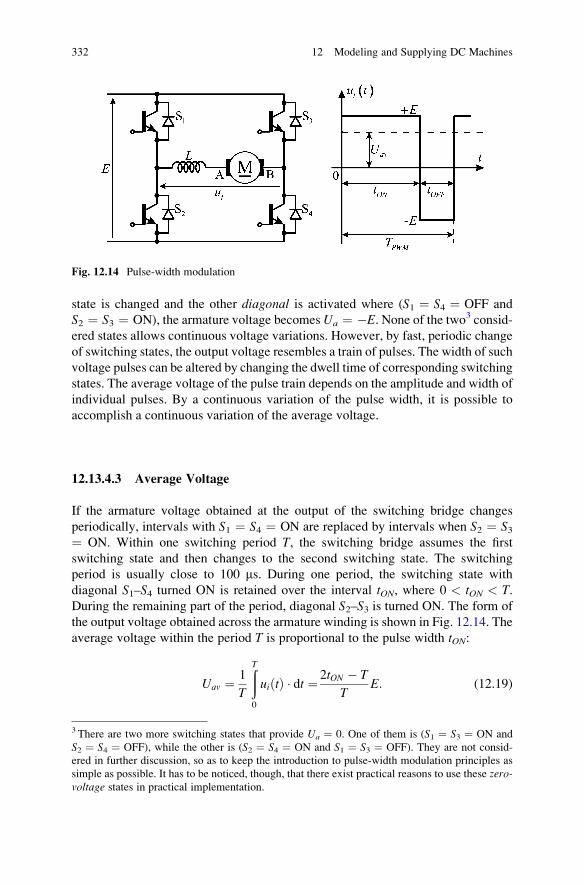
state is changed and the other diagonal is activated where (S1 ¼ S4 ¼ OFF and
S2 ¼ S3 ¼ ON), the armature voltage becomes Ua ¼ �E. None of the two3 consid-ered states allows continuous voltage variations. However, by fast, periodic change
of switching states, the output voltage resembles a train of pulses. The width of such
voltage pulses can be altered by changing the dwell time of corresponding switching
states. The average voltage of the pulse train depends on the amplitude and width of
individual pulses. By a continuous variation of the pulse width, it is possible to
accomplish a continuous variation of the average voltage.
12.13.4.3 Average Voltage
If the armature voltage obtained at the output of the switching bridge changes
periodically, intervals with S1 ¼ S4 ¼ ON are replaced by intervals when S2 ¼ S3¼ ON. Within one switching period T, the switching bridge assumes the first
switching state and then changes to the second switching state. The switching
period is usually close to 100 ms. During one period, the switching state with
diagonal S1–S4 turned ON is retained over the interval tON, where 0 < tON < T.During the remaining part of the period, diagonal S2–S3 is turned ON. The form of
the output voltage obtained across the armature winding is shown in Fig. 12.14. The
average voltage within the period T is proportional to the pulse width tON:
Uav ¼ 1
T
ðT
0
uiðtÞ � dt ¼ 2tON � T
TE: (12.19)
Fig. 12.14 Pulse-width modulation
3 There are two more switching states that provide Ua ¼ 0. One of them is (S1 ¼ S3 ¼ ON and
S2 ¼ S4 ¼ OFF), while the other is (S2 ¼ S4 ¼ ON and S1 ¼ S3 ¼ OFF). They are not consid-
ered in further discussion, so as to keep the introduction to pulse-width modulation principles as
simple as possible. It has to be noticed, though, that there exist practical reasons to use these zero-voltage states in practical implementation.
332 12 Modeling and Supplying DC Machines
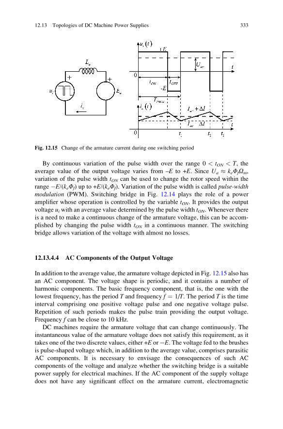
By continuous variation of the pulse width over the range 0 < tON < T, theaverage value of the output voltage varies from –E to +E. Since Ua � keFfOm,
variation of the pulse width tON can be used to change the rotor speed within the
range �E/(keFf) up to +E/(keFf). Variation of the pulse width is called pulse-widthmodulation (PWM). Switching bridge in Fig. 12.14 plays the role of a power
amplifier whose operation is controlled by the variable tON. It provides the output
voltage uiwith an average value determined by the pulse width tON. Whenever there
is a need to make a continuous change of the armature voltage, this can be accom-
plished by changing the pulse width tON in a continuous manner. The switching
bridge allows variation of the voltage with almost no losses.
12.13.4.4 AC Components of the Output Voltage
In addition to the average value, the armature voltage depicted in Fig. 12.15 also has
an AC component. The voltage shape is periodic, and it contains a number of
harmonic components. The basic frequency component, that is, the one with the
lowest frequency, has the period T and frequency f ¼ 1/T. The period T is the time
interval comprising one positive voltage pulse and one negative voltage pulse.
Repetition of such periods makes the pulse train providing the output voltage.
Frequency f can be close to 10 kHz.
DC machines require the armature voltage that can change continuously. The
instantaneous value of the armature voltage does not satisfy this requirement, as it
takes one of the two discrete values, either +E or�E. The voltage fed to the brushesis pulse-shaped voltage which, in addition to the average value, comprises parasitic
AC components. It is necessary to envisage the consequences of such AC
components of the voltage and analyze whether the switching bridge is a suitable
power supply for electrical machines. If the AC component of the supply voltage
does not have any significant effect on the armature current, electromagnetic
Fig. 12.15 Change of the armature current during one switching period
12.13 Topologies of DC Machine Power Supplies 333
torque, and the rotor speed, and it does not contribute to losses, then the operation of
an electrical machine supplied by the pulse-shaped voltage corresponds to
the operation of the same machine fed from an ideal voltage source providing the
voltage ua(t) ¼ (2tON � T)E/T which is pulse-free and does not have any AC
components.
12.13.4.5 Low-Pass Nature of Electrical Machines
The windings of electrical machines have certain inductance, determined by the
number of turns and the magnetic resistance. Impedance of the winding to electrical
currents of the angular frequency o is X ¼ Lo. In cases where an AC voltage is fed
to the winding, the amplitude of AC electrical currents caused by such voltage
decreases at elevated angular frequencies o. Therefore, at very large frequencies,
the impact of AC voltages on armature current is negligible.
Differential equation ua(t) ¼ Raia(t) + Ladia(t)/dt + Ea describes transient pro-
cesses in the armature winding. Laplace transform can be applied to obtain the
equation Ua(s) ¼ RaIa(s) + sLaIa(s) + Ea(s) with complex images of voltages and
currents. The armature current is obtained as Ia(s) ¼ (Ua(s) � Ea(s))/(Ra + sLa).The function W(s) ¼ 1/(Ra + sLa) represents transfer function of the armature
winding, and it describes the response of the armature current to changes in the
armature voltage. The transfer function is obtained by dividing the complex images
of relevant currents and voltages. Since the armature voltage is the cause while the
armature current change is the consequence, the voltage is considered an input and
the current an output. The function W(s) is used to establish the response of
armature current to the excitation by armature voltage, wherein the latter comprises
certain harmonic components. The ratio of currents I(jo) and voltagesU(jo) havingcertain angular frequency o ¼ 2p/T is obtained by replacing s ¼ jo in W(s):
I joð ÞU joð Þ ¼ W joð Þ ¼ 1
Ra þ joLa� 1
joLa: (12.20)
At frequencies of the order of several kHz, it is justified to assume that Ra �oLa; thus, the ratio of AC components of currents and voltages is determined as
1/(Lao). Therefore, the voltage components at higher frequencies produce corres-
ponding components of the armature current with rather small amplitude. At
frequencies of the order of 10 kHz, reactance Lao is so high that the response of
the armature current is negligible. Therefore, the pulsating nature of the supply
voltage has no significant effect on the armature current. Therefore, for all practical
uses, the presence of AC components in the armature voltage can be neglected.
Therefore, the analysis of operation of DC machines fed from PWM-controlled
switching bridge supplies can be simplified by modeling the switching bridge in a
way that omits the high-frequency AC components. If the switching frequency
f ¼ 1/T is sufficiently high, the switching supply shown in Fig. 12.12 can be
334 12 Modeling and Supplying DC Machines
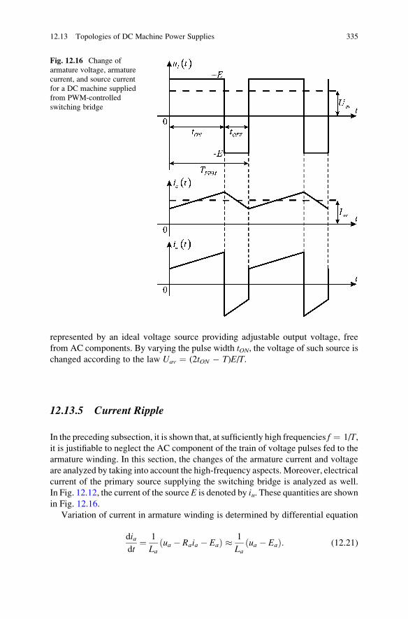
represented by an ideal voltage source providing adjustable output voltage, free
from AC components. By varying the pulse width tON, the voltage of such source ischanged according to the law Uav ¼ (2tON � T)E/T.
12.13.5 Current Ripple
In the preceding subsection, it is shown that, at sufficiently high frequencies f ¼ 1/T,it is justifiable to neglect the AC component of the train of voltage pulses fed to the
armature winding. In this section, the changes of the armature current and voltage
are analyzed by taking into account the high-frequency aspects. Moreover, electrical
current of the primary source supplying the switching bridge is analyzed as well.
In Fig. 12.12, the current of the source E is denoted by iu. These quantities are shownin Fig. 12.16.
Variation of current in armature winding is determined by differential equation
diadt
¼ 1
Laua � Raia � Eað Þ � 1
Laua � Eað Þ: (12.21)
Fig. 12.16 Change of
armature voltage, armature
current, and source current
for a DC machine supplied
from PWM-controlled
switching bridge
12.13 Topologies of DC Machine Power Supplies 335
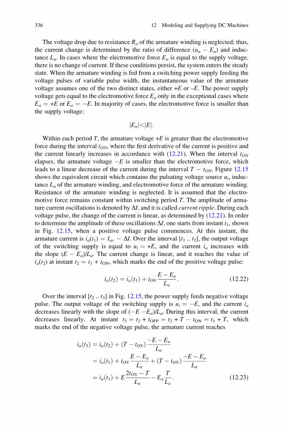
The voltage drop due to resistance Ra of the armature winding is neglected; thus,
the current change is determined by the ratio of difference (ua � Ea) and induc-
tance La. In cases where the electromotive force Ea is equal to the supply voltage,
there is no change of current. If these conditions persist, the system enters the steady
state. When the armature winding is fed from a switching power supply feeding the
voltage pulses of variable pulse width, the instantaneous value of the armature
voltage assumes one of the two distinct states, either +E or –E. The power supplyvoltage gets equal to the electromotive force Ea only in the exceptional cases where
Ea ¼ +E or Ea ¼ �E. In majority of cases, the electromotive force is smaller than
the supply voltage:
Eaj j< Ej j:Within each period T, the armature voltage +E is greater than the electromotive
force during the interval tON, where the first derivative of the current is positive andthe current linearly increases in accordance with (12.21). When the interval tONelapses, the armature voltage �E is smaller than the electromotive force, which
leads to a linear decrease of the current during the interval T � tON. Figure 12.15
shows the equivalent circuit which contains the pulsating voltage source ui, induc-tance La of the armature winding, and electromotive force of the armature winding.
Resistance of the armature winding is neglected. It is assumed that the electro-
motive force remains constant within switching period T. The amplitude of arma-
ture current oscillations is denoted by DI, and it is called current ripple. During eachvoltage pulse, the change of the current is linear, as determined by (12.21). In order
to determine the amplitude of these oscillations DI, one starts from instant t1, shownin Fig. 12.15, when a positive voltage pulse commences. At this instant, the
armature current is ia(t1) ¼ Iav � DI. Over the interval [t1 .. t2], the output voltageof the switching supply is equal to ui ¼ +E, and the current ia increases with
the slope (E � Ea)/La. The current change is linear, and it reaches the value of
ia(t2) at instant t2 ¼ t1 + tON, which marks the end of the positive voltage pulse:
ia t2ð Þ ¼ ia t1ð Þ þ tONE� Ea
La: (12.22)
Over the interval [t2 .. t3] in Fig. 12.15, the power supply feeds negative voltage
pulse. The output voltage of the switching supply is ui ¼ �E, and the current iadecreases linearly with the slope of (�E �Ea)/La. During this interval, the current
decreases linearly. At instant t3 ¼ t2 + tOFF ¼ t2 + T � tON ¼ t1 + T, which
marks the end of the negative voltage pulse, the armature current reaches
ia t3ð Þ ¼ ia t2ð Þ þ T � tONð Þ�E� Ea
La
¼ ia t1ð Þ þ tONE� Ea
Laþ T � tONð Þ�E� Ea
La
¼ ia t1ð Þ þ E2tON � T
La� Ea
T
La: (12.23)
336 12 Modeling and Supplying DC Machines
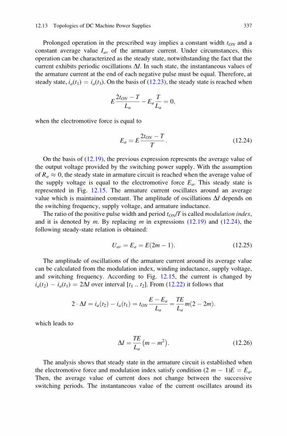
Prolonged operation in the prescribed way implies a constant width tON and a
constant average value Iav of the armature current. Under circumstances, this
operation can be characterized as the steady state, notwithstanding the fact that the
current exhibits periodic oscillations DI. In such state, the instantaneous values of
the armature current at the end of each negative pulse must be equal. Therefore, at
steady state, ia(t1) ¼ ia(t3). On the basis of (12.23), the steady state is reached when
E2tON � T
La� Ea
T
La¼ 0;
when the electromotive force is equal to
Ea ¼ E2tON � T
T: (12.24)
On the basis of (12.19), the previous expression represents the average value of
the output voltage provided by the switching power supply. With the assumption
of Ra � 0, the steady state in armature circuit is reached when the average value of
the supply voltage is equal to the electromotive force Ea. This steady state is
represented in Fig. 12.15. The armature current oscillates around an average
value which is maintained constant. The amplitude of oscillations DI depends onthe switching frequency, supply voltage, and armature inductance.
The ratio of the positive pulse width and period tON/T is calledmodulation index,and it is denoted by m. By replacing m in expressions (12.19) and (12.24), the
following steady-state relation is obtained:
Uav ¼ Ea ¼ E 2m� 1ð Þ: (12.25)
The amplitude of oscillations of the armature current around its average value
can be calculated from the modulation index, winding inductance, supply voltage,
and switching frequency. According to Fig. 12.15, the current is changed by
ia(t2) � ia(t1) ¼ 2DI over interval [t1 .. t2]. From (12.22) it follows that
2 � DI ¼ ia t2ð Þ � ia t1ð Þ ¼ tONE� Ea
La¼ TE
Lam 2� 2mð Þ:
which leads to
DI ¼ TE
Lam� m2� �
: (12.26)
The analysis shows that steady state in the armature circuit is established when
the electromotive force and modulation index satisfy condition (2 m � 1)E ¼ Ea.
Then, the average value of current does not change between the successive
switching periods. The instantaneous value of the current oscillates around its
12.13 Topologies of DC Machine Power Supplies 337
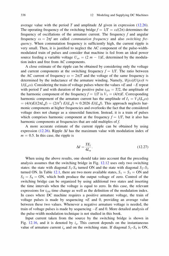
average value with the period T and amplitude DI given in expression (12.26).
The operating frequency of the switching bridge f ¼ 1/T ¼ o/(2p) determines the
frequency of oscillations of the armature current. The frequency f and angular
frequency o ¼ 2pf are called commutation frequency and also switching fre-quency. When commutation frequency is sufficiently high, the current ripple is
very small. Then, it is justified to neglect the AC component of the pulse-width-
modulated train of pulses and consider that machine is fed from an ideal power
source feeding a variable voltage Uav ¼ (2 m � 1)E, determined by the modula-
tion index and free from AC components.
A close estimate of the ripple can be obtained by considering only the voltage
and current components at the switching frequency f ¼ 1/T. The ratio between
the AC current of frequency o ¼ 2p/T and the voltage of the same frequency is
determined by the inductance of the armature winding. Namely, |I(jo)/U(jo)| �1/(Lao). Considering the train of voltage pulses where the values +E and �E repeat
with period T and with duration of the positive pulse tON ¼ T/2, the amplitude of
the harmonic component of the frequency f ¼ 1/T is V1 ¼ (4/p)E. Correspondingharmonic component of the armature current has the amplitude of I1 ¼ V1/(Lao)¼ (4/p)E/(2pLaf) ¼ (2/p2) E/(Laf) � 0.2026 E/(Laf). This approach neglects har-
monic components at higher frequencies and overlooks the fact that the considered
voltage does not change as a sinusoidal function. Instead, it is a train of pulses
which comprises harmonic component at the frequency f ¼ 1/T, but it also has
harmonic components at frequencies that are odd multiples of f.A more accurate estimate of the current ripple can be obtained by using
expression (12.26). Ripple DI has the maximum value with modulation index of
m ¼ 0.5. In this case, the ripple is
DI ¼ TEi
4La: (12.27)
When using the above results, one should take into account that the preceding
analysis assumes that the switching bridge in Fig. 12.12 uses only two switching
states: the state with diagonal S1-S4 turned ON and the state with diagonal S2–S3turned ON. In Table 12.1, there are two more available states, S1 ¼ S3 ¼ ON and
S2 ¼ S4 ¼ ON, which both produce the output voltage of zero. Control of the
switching bridge can be organized by using additional two states and inserting
the time intervals when the voltage is equal to zero. In this case, the relevant
expressions for tON time change as well as the definition of the modulation index.
In cases where DC machine requires a positive armature voltage, the train of
voltage pulses is made by sequencing +E and 0, providing an average value
between these two values. Whenever a negative armature voltage is needed, the
train of voltage pulses is made by sequencing �E and 0. More detailed analysis of
the pulse-width modulation technique is not studied in this book.
Input current taken from the source by the switching bridge is shown in
Fig. 12.16, and it is denoted by iu. This current depends on the instantaneous
value of armature current ia and on the switching state. If diagonal S1–S4 is ON,
338 12 Modeling and Supplying DC Machines
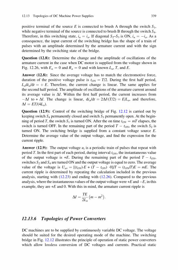
positive terminal of the source E is connected to brush A through the switch S1,while negative terminal of the source is connected to brush B through the switch S4.Therefore, in this switching state, iu ¼ ia. If diagonal S2–S3 is ON, iu ¼ �ia. As aconsequence, the input current of the switching bridge has the shape of a train of
pulses with an amplitude determined by the armature current and with the sign
determined by the switching state of the bridge.
Question (12.8): Determine the change and the amplitude of oscillations of the
armature current in the case when DC motor is supplied from the voltage shown in
Fig. 12.26, with Ea ¼ 0 and Ra ¼ 0 and with known La, T, and E.
Answer (12.8): Since the average voltage has to match the electromotive force,
duration of the positive voltage pulse is tON ¼ T/2. During the first half period,
Ladia/dt ¼ þ E. Therefore, the current change is linear. The same applies for
the second half period. The amplitude of oscillations of the armature current around
its average value is DI. Within the first half period, the current increases from
�DI to + DI. The change is linear, dia/dt ¼ 2DI/(T/2) ¼ E/La, and therefore,
DI ¼ ET/(4La).
Question (12.9): Control of the switching bridge of Fig. 12.12 is carried out by
keeping switch S4 permanently closed and switch S3 permanently open. At the begin-
ning of period T, the switch S1 is turned ON. After the on time tON ¼ mT elapses, the
switch is turned OFF. In the remaining part of the period T � tON, the switch S2 isturned ON. The switching bridge is supplied from a constant voltage source E.Determine the average value of the output voltage, and find the expression for the
current ripple.
Answer (12.9): The output voltage ui is a periodic train of pulses that repeat with
period T. In the first part of each period, during interval tON, the instantaneous valueof the output voltage is +E. During the remaining part of the period T � tON,switches S2 and S4 are turned ON and the output voltage is equal to zero. The average
value of the voltage is Uav ¼ [(tON)�E + (T � tON) �0]/T ¼ (tON/T)E ¼ mE. Thecurrent ripple is determined by repeating the calculation included in the previous
analysis, starting with (12.23) and ending with (12.26). Compared to the previous
analysis, where the instantaneous values of the output voltagewere +E and�E, in thisexample, they are +E and 0. With this in mind, the armature current ripple is
DI ¼ TE
2Lam� m2� �
:
12.13.6 Topologies of Power Converters
DC machines are to be supplied by continuously variable DC voltage. The voltage
should be suited for the desired operating mode of the machine. The switching
bridge in Fig. 12.12 illustrates the principle of operation of static power converters
which allow lossless conversion of DC voltages and currents. Practical static
12.13 Topologies of DC Machine Power Supplies 339
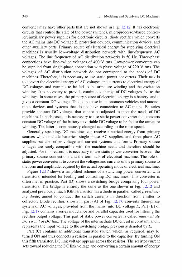
converter may have other parts that are not shown in Fig. 12.12. It has electronic
circuits that control the state of the power switches, microprocessor-based control-
ler, auxiliary power supplies for electronic circuits, diode rectifier which converts
the AC mains into DC voltage E, protection devices, communication devices, and
other auxiliary parts. Primary source of electrical energy for supplying electrical
machines is usually low-voltage distribution network with line-frequency AC
voltages. The line frequency of AC distribution networks is 50 Hz. Three-phase
connections have line-to-line voltages of 400 V rms. Low-power converters can
be supplied from single-phase connection with phase voltage of 220 V rms. The
voltages of AC distribution network do not correspond to the needs of DC
machines. Therefore, it is necessary to use static power converters. Their task is
to convert the electrical energy of AC voltages and currents to electrical energy of
DC voltages and currents to be fed to the armature winding and the excitation
winding. It is necessary to provide continuous change of DC voltages fed to the
windings. In some cases, the primary source of electrical energy is a battery, and it
gives a constant DC voltage. This is the case in autonomous vehicles and autono-
mous devices and systems that do not have connection to AC mains. Batteries
provide constant DC voltages that cannot be adjusted to meet the needs of DC
machines. In such cases, it is necessary to use static power converter that converts
constant DC voltage of the battery to variable DC voltage to be fed to the armature
winding. The latter is continuously changed according to the rotor speed.
Generally speaking, DC machines can receive electrical energy from primary
sources which include batteries, single-phase AC supplies, and three-phase AC
supplies but also other voltage and current systems and forms. Primary source
voltages are rarely compatible with the machine needs and therefore should be
adjusted. For this reason, it is necessary to use static power converter between the
primary source connections and the terminals of electrical machine. The role of
static power converter is to convert the voltages and currents of the primary source to
the form and amplitude required by the actual operating mode of electrical machine.
Figure 12.17 shows a simplified scheme of a switching power converter with
transistors, intended for feeding and controlling DC machines. This converter is
often met in practice. Part (D) shows a switching bridge comprising four power
transistors. The bridge is entirely the same as the one shown in Fig. 12.12 and
analyzed previously. Each IGBT transistor has a diode in parallel, called freewheel-ing diode, aimed to conduct the switch currents in direction from emitter to
collector. Diode rectifier, shown in part (A) of Fig. 12.17, converts three-phase
system of AC voltages, provided from the mains, into DC voltage E. Part (B) ofFig. 12.17 contains a series inductance and parallel capacitor used for filtering the
rectifier output voltage. This part of static power converter is called intermediateDC circuit or DC link. The voltage of the intermediate DC circuit is constant, and it
represents the input voltage to the switching bridge, previously denoted by E.Part (C) contains an additional transistor switch which, as required, may be
turned ON and thus connects a resistor in parallel to the capacitor. By turning ON
this fifth transistor, DC link voltage appears across the resistor. The resistor current
acts toward reducing the DC link voltage and converting a certain amount of energy
340 12 Modeling and Supplying DC Machines
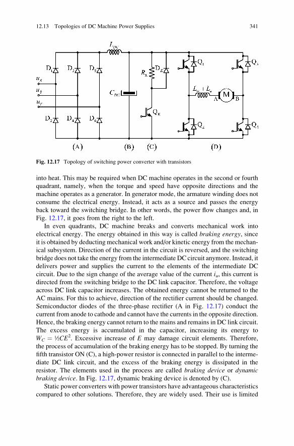
into heat. This may be required when DC machine operates in the second or fourth
quadrant, namely, when the torque and speed have opposite directions and the
machine operates as a generator. In generator mode, the armature winding does not
consume the electrical energy. Instead, it acts as a source and passes the energy
back toward the switching bridge. In other words, the power flow changes and, in
Fig. 12.17, it goes from the right to the left.
In even quadrants, DC machine breaks and converts mechanical work into
electrical energy. The energy obtained in this way is called braking energy, sinceit is obtained by deducting mechanical work and/or kinetic energy from the mechan-
ical subsystem. Direction of the current in the circuit is reversed, and the switching
bridge does not take the energy from the intermediate DC circuit anymore. Instead, it
delivers power and supplies the current to the elements of the intermediate DC
circuit. Due to the sign change of the average value of the current iu, this current isdirected from the switching bridge to the DC link capacitor. Therefore, the voltage
across DC link capacitor increases. The obtained energy cannot be returned to the
AC mains. For this to achieve, direction of the rectifier current should be changed.
Semiconductor diodes of the three-phase rectifier (A in Fig. 12.17) conduct the
current from anode to cathode and cannot have the currents in the opposite direction.
Hence, the braking energy cannot return to the mains and remains in DC link circuit.
The excess energy is accumulated in the capacitor, increasing its energy to
WC ¼ ½CE2. Excessive increase of E may damage circuit elements. Therefore,
the process of accumulation of the braking energy has to be stopped. By turning the
fifth transistor ON (C), a high-power resistor is connected in parallel to the interme-
diate DC link circuit, and the excess of the braking energy is dissipated in the
resistor. The elements used in the process are called braking device or dynamicbraking device. In Fig. 12.17, dynamic braking device is denoted by (C).
Static power converters with power transistors have advantageous characteristics
compared to other solutions. Therefore, they are widely used. Their use is limited
Fig. 12.17 Topology of switching power converter with transistors
12.13 Topologies of DC Machine Power Supplies 341
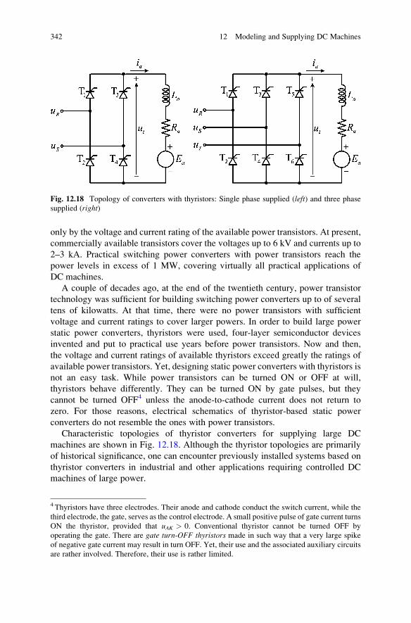
only by the voltage and current rating of the available power transistors. At present,
commercially available transistors cover the voltages up to 6 kV and currents up to
2–3 kA. Practical switching power converters with power transistors reach the
power levels in excess of 1 MW, covering virtually all practical applications of
DC machines.
A couple of decades ago, at the end of the twentieth century, power transistor
technology was sufficient for building switching power converters up to of several
tens of kilowatts. At that time, there were no power transistors with sufficient
voltage and current ratings to cover larger powers. In order to build large power
static power converters, thyristors were used, four-layer semiconductor devices
invented and put to practical use years before power transistors. Now and then,
the voltage and current ratings of available thyristors exceed greatly the ratings of
available power transistors. Yet, designing static power converters with thyristors is
not an easy task. While power transistors can be turned ON or OFF at will,
thyristors behave differently. They can be turned ON by gate pulses, but they
cannot be turned OFF4 unless the anode-to-cathode current does not return to
zero. For those reasons, electrical schematics of thyristor-based static power
converters do not resemble the ones with power transistors.
Characteristic topologies of thyristor converters for supplying large DC
machines are shown in Fig. 12.18. Although the thyristor topologies are primarily
of historical significance, one can encounter previously installed systems based on
thyristor converters in industrial and other applications requiring controlled DC
machines of large power.
Fig. 12.18 Topology of converters with thyristors: Single phase supplied (left) and three phase
supplied (right)
4 Thyristors have three electrodes. Their anode and cathode conduct the switch current, while the
third electrode, the gate, serves as the control electrode. A small positive pulse of gate current turns
ON the thyristor, provided that uAK > 0. Conventional thyristor cannot be turned OFF by
operating the gate. There are gate turn-OFF thyristors made in such way that a very large spike
of negative gate current may result in turn OFF. Yet, their use and the associated auxiliary circuits
are rather involved. Therefore, their use is rather limited.
342 12 Modeling and Supplying DC Machines
Chapter 13
Characteristics of DC Machines
WorkingwithDCmachines requires the knowledge on their electrical andmechanical
properties, parameters, and limitations. This chapter introduces and explains the
concept of rated quantities and discusses the maximum permissible currents in
continuous, steady-state service of DC machines. It also defines the safe operating
area of DC machines in Tem–Om plane, both in steady-state operation and during
transients. For the sake of readers that meet electrical machines for the first time,
the concepts of rated1 current, rated voltage, mechanical characteristics, natural
characteristics, rated speed, rated torque, and rated power are introduced and
explained in this chapter. The need to use machines at higher speeds and with reduced
flux is discussed and explained, introducing at the same time the constant flux
operating region and the field-weakening operating region. The problems of removing
the heat caused by the conversion losses are analyzed along with the performance
restrictions imposed by temperature limits. Besides, an insight is given into possible
short-term overload operation of DC machines. Principal conversion losses in DC
machines are analyzed, discussed, and included in power balance. This chapter closes
by discussing permissible operating areas in torque-speed plane. The steady-state safe
operating area in Tem–Om plane is also called exploitation characteristics. It is
introduced and explained along with the transient safe operating area, also called the
transient characteristic. Discussion and examples within this chapter are focused on
separately excited DC machines.
1 In electrical engineering, the concept of rated voltages, currents, and other similar quantities is
widely used. Considered quantities are usually the ones that contribute to thermal, mechanical,
dielectric, or other stress that may have potential of damaging electrical machine, transformer, or
other electrical device or to increase its ware and reduce the expected lifetime. The rated value is
most usually set by the manufacturer as a maximum value to be used with the considered device.
Continued operation with voltages and currents that exceed the rated values causes permanent
damage to machine windings, magnetic circuits, or other vital parts. For some quantities such as
electrical current, the rated value can be surpassed during very short intervals of time without
causing damages. The rated values are usually set somewhat below the level that damages the
device. This is done to allow a certain safety margin.
S.N. Vukosavic, Electrical Machines, Power Electronics and Power Systems,
DOI 10.1007/978-1-4614-0400-2_13, # Springer Science+Business Media New York 2013
343
13.1 Rated Voltage
The winding rated voltage is the highest voltage that can be permanently applied to
the winding terminals without causing breakdown or accelerated aging of electrical
insulation. In some cases, the rated voltage can be briefly exceeded without causing
any harm.
Electrical insulation separates the winding conductor from the walls of the slot
where the conductor is placed. In addition, the electrical insulation separates this
conductor from other conductors. A loss of insulation leads to a short circuit
between individual conductors, between the winding terminals, as well as between
the winding and the magnetic circuit or the machine housing. Each of the accidents
mentioned results in permanent damage and interrupts the operation of the
machine. In most cases, it has to be sent to the workshop or repair service.
The electrical field which exists in insulation is proportional to the supply
voltage. The insulation is characterized by the rated voltage Un as well as by the
breakdown voltage Umax.
The breakdown voltage causes instantaneous damage of insulation. With break-
down voltage applied, the electrical field strength in critical parts of the insulation
material exceeds the dielectric strength of the material and destroys insulation.
Cumulative ionization of otherwise nonconductive dielectric provides a virtual
short circuit between two conductors, or between the winding terminals, or a short
circuit between the winding and earthed metal parts of the machine.
The rated voltage is lower than the breakdown voltage. Supplying the winding
with a voltage which is higher than the rated but lower than the breakdown voltage
does not necessarily lead to breakdown. Increased electrical field strength
established with voltages above the rated lead to accelerated degradation and
aging of the insulation material. This phenomenon reduces the expected lifetime
of the insulation. Insulation aging is related to electrical, chemical, and thermal
processes within dielectric materials. In most cases where the voltage is maintained
within the limits of the rated voltage, expected lifetime of insulation materials and
systems reaches 20 years. Continued operation with voltages exceeding the rated by
8% may halve the insulation lifetime.
13.2 Mechanical Characteristic
Mechanical characteristic is function T(O) orO(T) which gives relation between theangular speed of rotation and electromagnetic torque in steady-state operating
conditions, with no variations of the speed, current, or flux of electrical machine.
For separately excited DC machine, where the excitation winding and armature
windings have separate supply, mechanical characteristic is given by expression
Tem ¼ km FfUa
Ra� kmke F2
f
RaOm
344 13 Characteristics of DC Machines
13.3 Natural Characteristic
Natural characteristic is mechanical characteristic obtained in the case when all the
voltages fed to the machine are equal to the rated voltages.
13.4 Rated Current
Rated current In is the maximum permissible armature current in continuous
operation. Namely, it is the largest current that can be maintained permanently,
which at the same time does not cause any overheating, damages, faults, or
accelerated aging. In AC machines, the rated current implies the rms value of the
winding current.
Electrical currents in windings of electrical machine produce losses and develop
heat, increasing the temperature of conductors and insulation. Current in the
windings creates Joule losses which are proportional to the square of the current.
The temperature of the machine is increased in proportion to generated heat.
Increased temperature difference between the surface of an electrical machine and
the environment gives a rise to heat transfer from the machine to the environment.
The heat can be passed by conduction, convection, and radiation. Heat conduction
takes place through the machine parts that are in touch with cold external solids such
as the machine basis or flange. Heat convection relies on natural or forced streaming
of air along the machine sides. Heat radiation is electromagnetic process caused by
thermal motion of charged particles on the surface of electrical machine, and it
depends on absolute temperature. The heat radiated from a warm machine to cold
environment is larger than the heat absorbed by the machine due to radiation caused
by the environment.
When the surface temperature of electrical machine exceeds the temperature of
the environment, the heat is transferred to the environment, and the machine is
cooled. The power PT of the heat transfer defines how many joules of heat are
transferred in each second. The processes of the heat transfer are nonlinear. Yet, for
the range of temperatures encountered in operation of electrical machines, the power
PT can be considered proportional to the temperature difference, PT ¼ Dy /RT, where
RT is thermal resistance of an electrical machine with respect to the environment,
proportional to the surface of the machine and characteristics of this surface. Power
PT is expressed inW, temperature Dy in oC, while thermal resistance RT is expressed
in oC/W. The equilibrium is established when the machine temperature reaches the
value that results in heat transfer PT which is equal to the total losses within the
machine. Total losses of electrical machine are denoted by Pg. With PT ¼ Pg,
machine temperature remains constant. The higher the losses in amachine, the higher
the temperature reached in the steady state. Considering aDCmachine, an increase of
armature current Ia increases Joule effect losses. They are proportional to I2, and they
13.4 Rated Current 345
increase temperature of DC machine. Excessive temperature increase may damage
some critical machine parts, such as the insulation of the windings.
Electrical insulation is made of paper, fiberglass, lacquer, or other materials.
It separates copper conductors of machine windings from other conductive parts of
machine, as well as from other conductors, thus preventing short circuits of the
windings or their individual turns. The insulation can be damaged if temperature
exceeds the maximum permissible limit for given insulating material. The insula-
tion of thermal class A is damaged if the temperature exceeds 105 �C. For insulationof class F, the temperature limit is 155 �C. Therefore, DC machine with class F
insulation would have higher permissible temperatures and higher rated current.
When DC machine operates in steady state with the rated armature current, the
losses are expected to heat the machine up to the temperature limit. With currents in
excess to the rated, DC machine in continuous service would overheat. At the same
time, temperature would exceed the limits and damage insulation or some other
vital part of the machine. Other than insulation, there are other machine parts that
are sensitive to elevated temperatures. Permanent magnets, ferromagnetic
materials, and even the elements of steel construction of the machine could deteri-
orate and fail due to excessive temperatures. Ferromagnetic materials lose their
magnetic properties when heated up to Curie temperature. Permanent magnets
could be permanently damaged (demagnetized) by overheating. The elements of
steel construction such as the shaft and bearings could be damaged due to thermal
dilatation, changes of steel properties, and failure in lubrication of the bearing at
high temperatures.
The rated current In is the highest armature current Ia in continuous service that
does not cause any damage or fault and does not shorten the expected lifetime of the
machine.
13.5 Thermal Model and Intermittent Operation
Conversion losses in an electrical machine lead to an increase of temperature of the
magnetic circuit and windings. Machine is warmer than the environment, and it
transfers heat to the environment. If the heat generated by the losses within the
machine is equal to the heat transferred to the environment, the system is in steady-
state conditions, and the temperature does not change. The temperature remains
constant in cases where the heat generation remains in equilibrium with the heat
emission. In other words, the heating has to be equal to cooling in order to achieve aconstant temperature. The maximum permissible temperatures of vital parts of the
machine are determined by endurance of the electrical insulation, magnetic circuit,
windings, bearings, and housing. Variation of temperature in a machine is deter-
mined by thermal resistance RT and thermal capacity CT, the two machine
parameters discussed further on. The former determines the heat emission from
the machine into the environment, while the latter determines the heat accumulated
within the machine. If thermal capacity is sufficiently large, the machine can endure
346 13 Characteristics of DC Machines
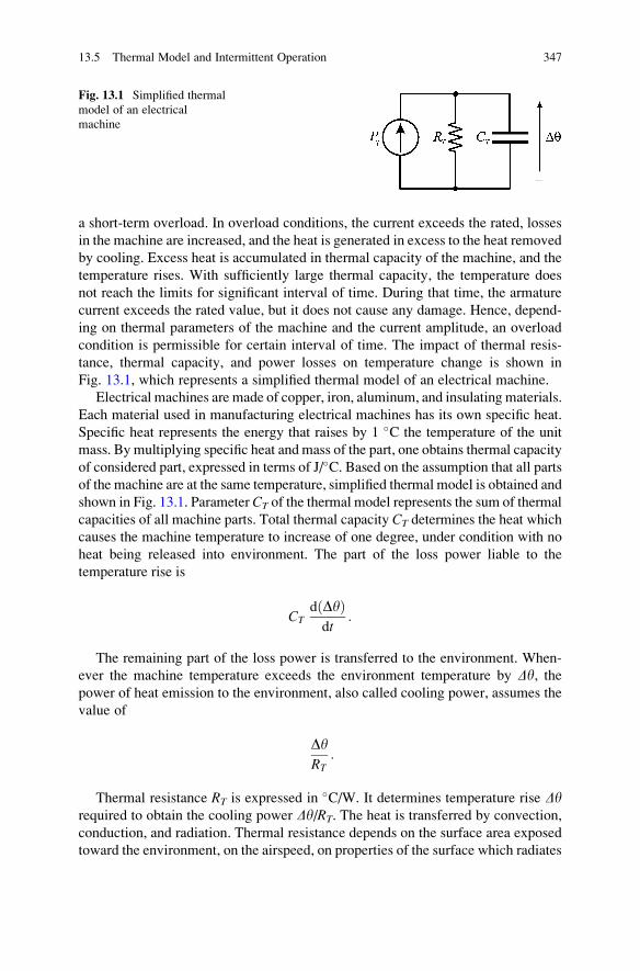
a short-term overload. In overload conditions, the current exceeds the rated, losses
in the machine are increased, and the heat is generated in excess to the heat removed
by cooling. Excess heat is accumulated in thermal capacity of the machine, and the
temperature rises. With sufficiently large thermal capacity, the temperature does
not reach the limits for significant interval of time. During that time, the armature
current exceeds the rated value, but it does not cause any damage. Hence, depend-
ing on thermal parameters of the machine and the current amplitude, an overload
condition is permissible for certain interval of time. The impact of thermal resis-
tance, thermal capacity, and power losses on temperature change is shown in
Fig. 13.1, which represents a simplified thermal model of an electrical machine.
Electrical machines are made of copper, iron, aluminum, and insulating materials.
Each material used in manufacturing electrical machines has its own specific heat.
Specific heat represents the energy that raises by 1 �C the temperature of the unit
mass. By multiplying specific heat and mass of the part, one obtains thermal capacity
of considered part, expressed in terms of J/�C. Based on the assumption that all parts
of the machine are at the same temperature, simplified thermal model is obtained and
shown in Fig. 13.1. Parameter CT of the thermal model represents the sum of thermal
capacities of all machine parts. Total thermal capacity CT determines the heat which
causes the machine temperature to increase of one degree, under condition with no
heat being released into environment. The part of the loss power liable to the
temperature rise is
CTd Dyð Þdt
:
The remaining part of the loss power is transferred to the environment. When-
ever the machine temperature exceeds the environment temperature by Dy, thepower of heat emission to the environment, also called cooling power, assumes the
value of
DyRT
:
Thermal resistance RT is expressed in �C/W. It determines temperature rise Dyrequired to obtain the cooling power Dy/RT. The heat is transferred by convection,
conduction, and radiation. Thermal resistance depends on the surface area exposed
toward the environment, on the airspeed, on properties of the surface which radiates
Fig. 13.1 Simplified thermal
model of an electrical
machine
13.5 Thermal Model and Intermittent Operation 347
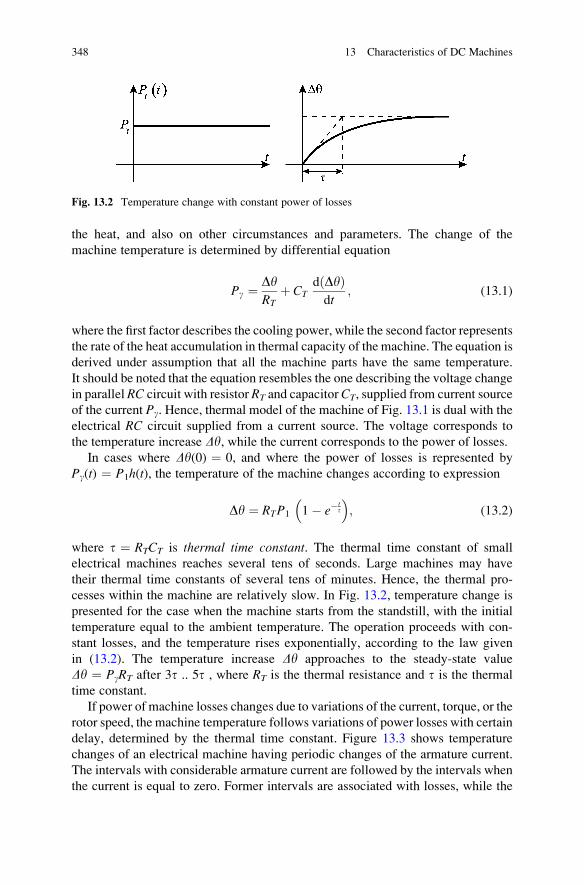
the heat, and also on other circumstances and parameters. The change of the
machine temperature is determined by differential equation
Pg ¼ DyRT
þ CTd Dyð Þdt
; (13.1)
where the first factor describes the cooling power, while the second factor represents
the rate of the heat accumulation in thermal capacity of the machine. The equation is
derived under assumption that all the machine parts have the same temperature.
It should be noted that the equation resembles the one describing the voltage change
in parallel RC circuit with resistor RT and capacitorCT, supplied from current source
of the current Pg. Hence, thermal model of the machine of Fig. 13.1 is dual with the
electrical RC circuit supplied from a current source. The voltage corresponds to
the temperature increase Dy, while the current corresponds to the power of losses.In cases where Dy(0) ¼ 0, and where the power of losses is represented by
Pg(t) ¼ P1h(t), the temperature of the machine changes according to expression
Dy ¼ RTP1 1� e�tt
� �; (13.2)
where t ¼ RTCT is thermal time constant. The thermal time constant of small
electrical machines reaches several tens of seconds. Large machines may have
their thermal time constants of several tens of minutes. Hence, the thermal pro-
cesses within the machine are relatively slow. In Fig. 13.2, temperature change is
presented for the case when the machine starts from the standstill, with the initial
temperature equal to the ambient temperature. The operation proceeds with con-
stant losses, and the temperature rises exponentially, according to the law given
in (13.2). The temperature increase Dy approaches to the steady-state value
Dy ¼ PgRT after 3t .. 5t , where RT is the thermal resistance and t is the thermal
time constant.
If power of machine losses changes due to variations of the current, torque, or the
rotor speed, the machine temperature follows variations of power losses with certain
delay, determined by the thermal time constant. Figure 13.3 shows temperature
changes of an electrical machine having periodic changes of the armature current.
The intervals with considerable armature current are followed by the intervals when
the current is equal to zero. Former intervals are associated with losses, while the
Fig. 13.2 Temperature change with constant power of losses
348 13 Characteristics of DC Machines
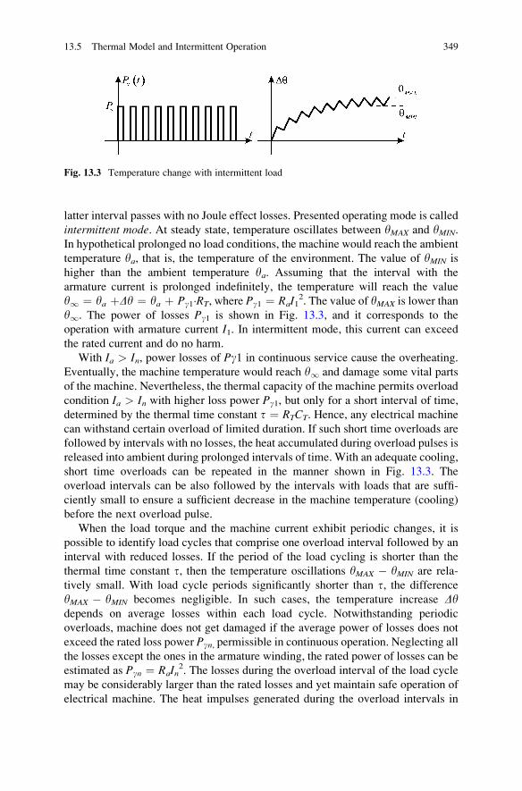
latter interval passes with no Joule effect losses. Presented operating mode is called
intermittent mode. At steady state, temperature oscillates between yMAX and yMIN.
In hypothetical prolonged no load conditions, the machine would reach the ambient
temperature ya, that is, the temperature of the environment. The value of yMIN is
higher than the ambient temperature ya. Assuming that the interval with the
armature current is prolonged indefinitely, the temperature will reach the value
y1 ¼ ya þDy ¼ ya þ Pg1�RT, where Pg1 ¼ RaI12. The value of yMAX is lower than
y1. The power of losses Pg1 is shown in Fig. 13.3, and it corresponds to the
operation with armature current I1. In intermittent mode, this current can exceed
the rated current and do no harm.
With Ia > In, power losses of Pg1 in continuous service cause the overheating.
Eventually, the machine temperature would reach y1 and damage some vital parts
of the machine. Nevertheless, the thermal capacity of the machine permits overload
condition Ia > In with higher loss power Pg1, but only for a short interval of time,
determined by the thermal time constant t ¼ RTCT. Hence, any electrical machine
can withstand certain overload of limited duration. If such short time overloads are
followed by intervals with no losses, the heat accumulated during overload pulses is
released into ambient during prolonged intervals of time. With an adequate cooling,
short time overloads can be repeated in the manner shown in Fig. 13.3. The
overload intervals can be also followed by the intervals with loads that are suffi-
ciently small to ensure a sufficient decrease in the machine temperature (cooling)
before the next overload pulse.
When the load torque and the machine current exhibit periodic changes, it is
possible to identify load cycles that comprise one overload interval followed by an
interval with reduced losses. If the period of the load cycling is shorter than the
thermal time constant t, then the temperature oscillations yMAX � yMIN are rela-
tively small. With load cycle periods significantly shorter than t, the difference
yMAX � yMIN becomes negligible. In such cases, the temperature increase Dydepends on average losses within each load cycle. Notwithstanding periodic
overloads, machine does not get damaged if the average power of losses does not
exceed the rated loss power Pgn, permissible in continuous operation. Neglecting all
the losses except the ones in the armature winding, the rated power of losses can be
estimated as Pgn ¼ RaIn2. The losses during the overload interval of the load cycle
may be considerably larger than the rated losses and yet maintain safe operation of
electrical machine. The heat impulses generated during the overload intervals in
Fig. 13.3 Temperature change with intermittent load
13.5 Thermal Model and Intermittent Operation 349
Fig. 13.3 are released into the ambient during the intervals with reduced losses.
Intermittent temperature rise yMAX � yMIN during overloads is inversely propor-
tional to the thermal capacity CT.
Based on the performed analysis, it is concluded that the current of an electrical
machine may exceed the rated current during short time intervals, provided that the
overload intervals are much shorter compared to the thermal time constant of the
machine. The overload pulses can come as a train, provided that the light load
intervals in between secure sufficient cooling and sufficient drop of the machine
temperature prior to arrival of the next pulse. With load that comes as a train of
pulses, machine operation is safe if the repetition period is shorter than the thermal
time constant, and provided that the average power of losses does not exceed the
losses incurred with nominal current.
Question (13.1): While operating with the rated load, the steady-state temperature
of an electrical machine is only slightly increased above the ambient temperature. Is
it designed properly?
Answer (13.1): No. Small steady-state operating temperatures show that the
power of losses within the machine is rather small. This means that there is plenty
of room for increasing the current density and increasing the magnetic induction.
The flux increase accompanied by the increase in the armature current raises the
output torque and power. Hence, the machine under consideration can produce
significantly higher torque and power compared to the power declared as the rated.
Consequently, too much copper and too much iron are used to make the machine.
Other than being more expensive, the machine is also larger and heavier. The same
load requirements can be met by electrical machine of much smaller size and
weight.
Question (13.2): Electrical machine has not been used for a long time. After
turning on, the armature current reaches the value of 2In, twice the rated current.
Prevailing losses are the winding losses. These are proportional to the square of the
current. The iron losses can be neglected. The thermal time constant is 60s.
Determine the longest permissible time the machine can be operated with 2Inwith no damages.
Answer (13.2): Permanent operation with twice the rated current produces the
power of losses which is four times larger than the rated power of losses. Therefore,
the machine would heat up rather quickly. Theoretical value of the steady-state
temperature in this mode is four times higher than the permissible temperature. The
limit temperature is reached after t1, where 1 � exp(�t1/tT) ¼ ¼. It follows that
t1 ¼ 17.26 s.
Question (13.3): Electrical machine is loaded in such a way that every 10s a pulse
of armature current appears having the amplitude of 2In. This pulse is followed by
an interval with no current. Prevailing losses in the machine are the winding losses,
which are proportional to the square of the armature current, while the iron losses
can be neglected. It is known that the thermal time constant is tT � 10s. Determine
350 13 Characteristics of DC Machines
the longest permissible width of the armature current pulse which does not cause
damages to the machine.
Answer (13.3): Thermal time constant is significantly higher than the pulse period
(tT � 10 s). Therefore, temperature variations are slow, and the temperature
changes within the pulse period are insignificant. For that reason, it is possible to
consider the average power of losses. With any periodic current i(t), the average
power of Joule losses is calculated as
Pg avð Þ ¼ 1
T
ZT
0
Rai2adt ¼ Ra
1
T
ðT
0
i2adt
0@
1A ¼ RaIa rmsð Þ;
where Ia(rms) is the rms (root mean square) current. The rms current is also called
thermal equivalent of periodic current i(t). A resistor with constant Ia(rms) will heatup very much the same as it does with periodic current i(t). If the rms value does not
exceed the rated value In, the machine does not overheat. A pulse of amplitude 2Inthat repeats every 10 s has the rms value of In provided that the pulse width is 2.5 s.
13.6 Rated Flux
Excitation fluxFf determines the current which has to be established in the armature
winding so as to develop the desired torque, Ia ¼ Tem/(kmFf). With higher values of
flux, one and the same torque is obtained with lower armature current, and this
reduces the winding losses. Therefore, it is of interest to increase the flux in order to
reduce the required armature current. The excitation flux is limited by magnetic
saturation of the ferromagnetic material. If the region of saturation is reached, any
further increase of the excitation current results in a very small change of the flux.
While operating in saturation region, the only effect of increasing the excitation
current is the increase in power of excitation winding losses RfIf2. Magnetic satura-
tion becomes pronounced at the knee of themagnetizing curveFf(If). The knee of thecurve is the point where the initial, linear slope ends and the curve bends toward
the abscissa, resulting in very small DF/DIf ratio. The flux at the knee point is
denoted by Ffmax. Since any further increase of the excitation current is of little
practical effect, the value Ffmax represents the maximum flux. This flux can be used
in order to reduce the armature current Ia ¼ Tem/(kmFf) required to achieve desired
torque Tem. Analysis performed in subsequent sections shows that, in certain
operating conditions, the value ofFfmax cannot be used. An example is the operation
at very high speeds, where the electromotive force keFfOmmust not exceed the rated
voltage. In other cases, the flux Ffmax can be advantageously used, providing
reduction in armature current. The knee point flux Ffmax is also called rated flux,and it is denoted by Fn.
13.6 Rated Flux 351
13.7 Rated Speed
Rotor speed of electrical machine influences electromotive force induced in the
windings. Rated speed is defined as the rotor speed where electrical machine with
rated flux has electromotive forces equal to the rated voltage. Hence, when the
machine with rated flux accelerates from zero to the rated speed, the electromotive
forces increase from zero up to the rated voltage.
Electromotive forces should not exceed the rated voltage in order to avoid
excessive voltage that could damage the insulation. Therefore, definition of the
rated speed implies that the machine cannot exceed the rated speed yet maintaining
the rated flux. In order to contain the electromotive forces between the rated limits,
the flux has to be reduced as the speed goes beyond the rated speed.
Considering a DC machine with rated excitation flux and with a negligible
resistance Ra, the electromotive force Ea ¼ keFnOm is induced, equal to the arma-
ture voltage Ua. At the rated speed, the electromotive force is equal to the rated
voltage. Therefore, rated speed of DC machine is determined by relation
On ¼ Un
keFn(13.3)
Since the armature voltage should not exceed the rated value, the operation at
speeds larger than the rated is possible only with a reduced flux. Otherwise, the
electromotive force keFnOm would exceed the nominal voltage Un ¼ keFnOn.
For small electrical machines, the voltage drop due to winding resistances cannot
be neglected. Since Ua ¼ RaIa þ Ea, the difference between the armature voltage
and the electromotive force cannot be neglected. In such cases, definition of rated
speed is made more precise, and it includes the voltage drop across the armature
resistance. The rated speed can be defined as the one that results in rated voltage
across the armature winding of electrical machine which operates with the rated
flux and the rated current. In such conditions, the electromotive force is equal to
Ea ¼ keFnOn ¼ Un � RaIn, while the rated speed is defined by expression
On ¼ Un � RaInkeFn
: (13.4)
13.8 Field Weakening
Operation of DC machines may require changes in the excitation flux. One example
is the operation at speeds above the rated speed. In order to keep the electromotive
force within the limits of the rated voltage, the flux should be reduced so as to
maintain the relation keFnOm < Un. Flux reduction at high speeds is called fieldweakening.
352 13 Characteristics of DC Machines
In addition, there are cases when the flux reduction is beneficial even at speeds
below the rated. When electrical machine runs with relatively low electromagnetic
torque, current is also low, as well as the power of losses in the winding. If at the
same time the flux is kept at the rated value, the iron losses in the magnetic circuit
become the principal conversion losses. In order to reduce the losses, it is necessary
to reduce the flux. Lowering the flux increases the armature current required to
develop desired torque, due to Ia ¼ Tem/(kmFf). Operation with low Tem allows for
relatively large flux reduction without any significant increase in armature current.
For this reason, flux reduction at light load condition reduces the conversion losses.
13.8.1 High-Speed Operation
The electromotive force induced in the winding determines the voltage across the
winding terminals. Therefore, the electromotive force must not exceed the rated
voltage. The rated flux, voltage and speed are related by Un � keFnOn. Therefore,
electrical machine running with the rated flux Fn has the electromotive force that
reaches the rated voltage as the speed approaches the rated speed. Any increase of
the speed above the rated would result in excessive voltages. Therefore, the
excitation flux has to be decreased as the rotor speed goes beyond On. Hence,
electrical machines can maintain the operating speed Om > On, provided that the
flux is reduced so as to prevent the electromotive force from exceeding the rated
voltage. For that to achieve, the flux should be varied according to the rotor speed.
This change can be described by the function F(Om). Below the rated speed,
F(Om) ¼ Fn.
At speeds Om > On, the electromotive force Ea ¼ ke�F(Om)�Om is induced in
the machine. Neglecting the armature resistance and assuming that Ea ¼ Un, the
flux to be used beyond the rated speed is
F Omð Þ F>Fnj ¼ Un
keOm: (13.5)
From expression (13.3), which defines the rated speed, one obtains
F Omð Þ ¼ FnOn
Om; (13.6)
which defines desired change of the flux at speeds above the rated speed. The flux is
inversely proportional to the speed and varies according to 1/Om. Variation of the
flux which is necessary at speeds beyond the rated speed is defined by (13.6).
The operating region where the speed is higher than the rated speed is called
field-weakening region. If machine operates at speeds below the rated speed, it is
possible to have the rated excitation flux Fn. For this reason, the operating region
where Om < On is called constant flux region.
13.8 Field Weakening 353
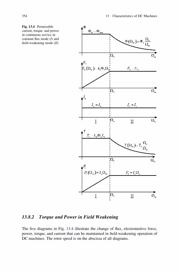
13.8.2 Torque and Power in Field Weakening
The five diagrams in Fig. 13.4 illustrate the change of flux, electromotive force,
power, torque, and current that can be maintained in field-weakening operation of
DC machines. The rotor speed is on the abscissa of all diagrams.
Fig. 13.4 Permissible
current, torque, and power
in continuous service in
constant flux mode (I) andfield-weakening mode (II)
354 13 Characteristics of DC Machines
It should be noted that diagrams in Fig. 13.4. represent the change in availablevalues or limit values, that is, the values that can be used at steady state without
causing any damage to the machine. Hence, any value below these limits can be used
as well. Due to thermal capacity of the machine, the instantaneous values of the
current, torque, and power may exceed the limit values for a brief interval of time. At
the same time, it is of interest to notice that presented diagram represents the absolute
values. The torque, current, and power may also take negative values. Therefore,
conclusions derived here are applicable to both motors and generators. Diagrams of
Fig. 13.4 and the corresponding conclusions are applicable to any machine studied
in this book, with exception of symbols which is slightly different for AC machine.
13.8.3 Flux Change
Abscissa of all the diagrams in Fig. 13.4 represents the rotor speed. At speeds below
the rated speed, the excitation flux is maintained at themaximumvalue, which is also
the rated value. As the speed exceeds the rated speed, the flux decreases according to
hyperbola F(Om) ¼ FnOn/Om. Machine can also use lower flux values, but they
cannot exceed the values shown by the curve F(Om).
13.8.4 Electromotive Force Change
The electromotive force varies according to the law Ea ¼ ke�F(Om)�Om. Below the
rated speed, the flux is equal to the rated flux, and the electromotive force increases
in proportion to the speed of rotation. In the region of the field weakening where
Om > On, the flux is inversely proportional to the rotor speed. If the speed
increases, the electromotive force remains constant and equal to the rated voltage.
If the flux is below the value determined by (13.5), the electromotive force will be
smaller than the rated voltage. In the region of field weakening, the flux F(Om) ¼FnOn/Om has to be applied. If, at the same time, machine operates with very small
torque and current, it is beneficial to reduce the flux even below the limit FnOn/Om,
so as to reduce the iron losses.
13.8.5 Current Change
At steady state, the armature current must not exceed its rated value, Ia2 � In
2.
The current can assume any value below the rated, |Ia| < In. Exceeding the rated
value in continuous operation results in overheating and may damage magnetic
and/or current circuits of the machine. For this reason, diagrams in Fig. 13.4
indicate that the armature current applicable over long time intervals is limited by
|Ia| < In at all speeds.
13.8 Field Weakening 355
13.8.6 Torque Change
Electromagnetic torque is determined by the product of the flux and current. During
long-term operation at speeds below the rated speed, the flux and current can hold
their rated values. Therefore, in these conditions, available electromagnetic torque
is Tn ¼ kmOnIn, also called rated torque. At speeds above the rated speed, the flux
decreases according to expression FnOn/Om. Therefore, the available torque in the
region of flux weakening is equal to T(Om) ¼ TnOn/Om. The product of torque
which decreases with the speed and the speed results in a constant power. For this
reason, the change of the available torque in the field-weakening mode is called
hyperbola of constant power.
13.8.7 Power Change
Electrical power converted to mechanical power is equal to the product of the torque
and the rotor speed. In constant flux region, at speeds below the rated, the available
torque is constant, thus the available power increases proportionally with the speed.
This region is also called the region of constant torque. In the region of field
weakening, the power is equal to the rated power Pn ¼ TnOn, since Pc ¼ TemOm ¼Om(TnOn/Om) ¼ TnOn ¼ Pn. Therefore, the available power in field-weakening
region is constant and equal to the rated power Pn. Another name for the field-
weakening region is the region of constant power. Power Pn is called rated power.
13.8.8 The Need for Field-Weakening Operation
Applications of electric motors often require high values of electromagnetic torque
at small speeds and small torques at high speeds. A DCmotor used for propulsion of
electrical vehicles can serve as an example. While setting in motion a heavily
loaded vehicle which has to manage a very steep slope, the motor has to deliver a
very large torque. In such case, it is important to develop the torque required to get
over the hill, while it is acceptable to operate the vehicle and the motor at a low
speed. The same vehicle may have to move unloaded over prolonged, flat path,
where the motion resistances are low, and where the motor delivers relatively small
torque. At the same time, it could be required to complete such motion quickly, and
this calls for high vehicle speeds and high rotor speeds.
The first example requires high-torque, low-speed operation, while the second
example calls for low-torque, high-speed operation. These requirements correspond
to a hyperbola T(O) in T–O plane. The curve T(Om) ¼ TnOn/Om is called hyperbola
of constant power. DC machines with permanent magnets cannot operate in the
field-weakening mode. There are no practical ways to reduce the flux of the
356 13 Characteristics of DC Machines
magnets. Therefore, these machines cannot go beyond the rated speed. Hence, the
constant power mode is inaccessible for this kind of DC machines. Whenever
the need exists for such machines to provide the constant power at high speed,
the problem cannot be solved on electrical side of the system. Instead, it is
necessary to use mechanical coupling with variable transmission ratio. In cases
when the electrical motor cannot increase the speed, as it has reached the rated rotor
speed, transmission ratio of mechanical coupling can be changed so as to obtain
higher load speeds with the same motor speed. Variable transmission ratio is used in
road vehicles as well. Automobiles with internal combustion engines (ICE) are
usually equipped with variable transmission gears. Torque-speed characteristics of
internal combustion engines do not include constant power range hyperbola in T(O)plane. In order to provide for both the low-speed, high-torque operation and the
high-speed, low-torque operation, it is necessary to change the transmission ratio of
the gears that pass the ICE torque to the wheels. The use of electrical machines
capable of providing constant power operation in field-weakening region removes
the need for additional gears.
13.9 Transient Characteristic
The transient characteristic is the area in T(O) plane which comprises all T–O points
attainable in short time intervals. That is, it is a collection of all the operating
regimes the machine can support for a short while. Peak values of the torque which
can be developed at a given speed depend on the excitation flux Ff(Om) and on
the peak value of the armature current. In DC machines, instantaneous value of the
current is limited by characteristics of mechanical commutator and on the maxi-
mum current of the semiconductor power switches used to build the switching
power converter that supplies the motor. An example of transient characteristic is
shown in Fig. 13.5.
13.10 Steady-State Operating Area
The steady-state operating area includes all the T-O points in T(O) plane where themachine can provide continuous service for a very long time. In the field-weakening
region, the area is limited by the hyperbola of constant power, Tem(Om) ¼ TnOn/Om,
while in the constant flux region the limit is Tem(Om) ¼ Tn. An example of steady-
state operating area is shown in Fig. 13.5. Since operation of electrical machines
includes all four quadrants, the steady-state operating area exists in all four
quadrants as well.
13.10 Steady-State Operating Area 357
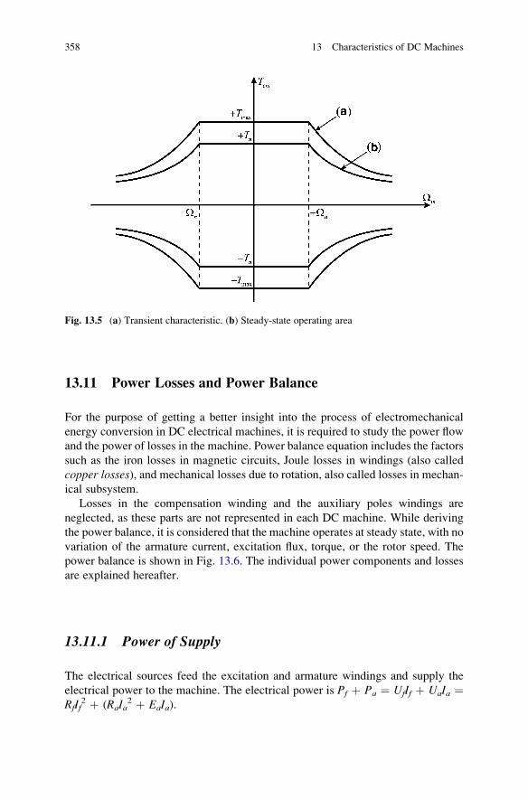
13.11 Power Losses and Power Balance
For the purpose of getting a better insight into the process of electromechanical
energy conversion in DC electrical machines, it is required to study the power flow
and the power of losses in the machine. Power balance equation includes the factors
such as the iron losses in magnetic circuits, Joule losses in windings (also called
copper losses), and mechanical losses due to rotation, also called losses in mechan-
ical subsystem.
Losses in the compensation winding and the auxiliary poles windings are
neglected, as these parts are not represented in each DC machine. While deriving
the power balance, it is considered that the machine operates at steady state, with no
variation of the armature current, excitation flux, torque, or the rotor speed. The
power balance is shown in Fig. 13.6. The individual power components and losses
are explained hereafter.
13.11.1 Power of Supply
The electrical sources feed the excitation and armature windings and supply the
electrical power to the machine. The electrical power is Pf þ Pa ¼ UfIf þ UaIa ¼RfIf
2 þ (RaIa2 þ EaIa).
Fig. 13.5 (a) Transient characteristic. (b) Steady-state operating area
358 13 Characteristics of DC Machines
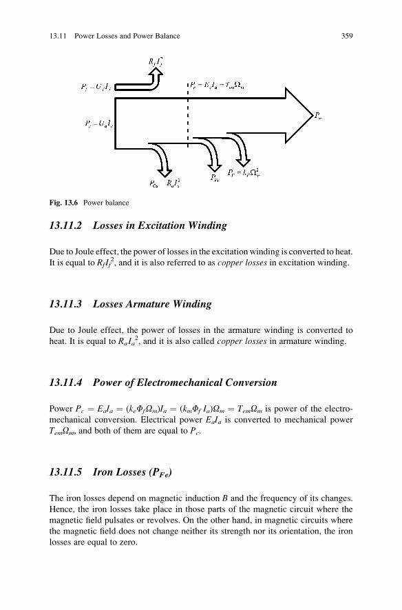
13.11.2 Losses in Excitation Winding
Due to Joule effect, the power of losses in the excitationwinding is converted to heat.
It is equal to RfIf2, and it is also referred to as copper losses in excitation winding.
13.11.3 Losses Armature Winding
Due to Joule effect, the power of losses in the armature winding is converted to
heat. It is equal to RaIa2, and it is also called copper losses in armature winding.
13.11.4 Power of Electromechanical Conversion
Power Pc ¼ EaIa ¼ (keFfOm)Ia ¼ (kmFf Ia)Om ¼ TemOm is power of the electro-
mechanical conversion. Electrical power EaIa is converted to mechanical power
TemOm, and both of them are equal to Pc.
13.11.5 Iron Losses (PFe)
The iron losses depend on magnetic induction B and the frequency of its changes.
Hence, the iron losses take place in those parts of the magnetic circuit where the
magnetic field pulsates or revolves. On the other hand, in magnetic circuits where
the magnetic field does not change neither its strength nor its orientation, the iron
losses are equal to zero.
Fig. 13.6 Power balance
13.11 Power Losses and Power Balance 359
In DC machines, the stator has the excitation winding with DC currents. Alter-
natively, permanent magnets are used instead of the excitation winding. In both
cases, consequential magnetic field within the stator magnetic circuit does not
change and, hence, does not produce the iron losses.
The rotor of a DC machine revolves in magnetic field of the excitation winding.
Therefore, magnetic induction revolves relative to the rotor magnetic circuit. The
frequency of changes of magnetic induction depends on the rotor speed. Due to
magnetic induction changes, there are iron losses due to hysteresis and losses due to
eddy currents. The iron losses have not been taken into account while developing
the mathematical model. Yet, it is of interest to include them in the power balance
equation. They are dependent on the square of the excitation flux, which determines
magnetic induction. In addition, the losses are dependent upon the speed of rotation,
because the field pulsates with respect to the iron sheets with a frequency which is
equal to the angular speed of the rotor. The iron losses within the rotor are denoted
by PFe. They exist even in cases when the armature winding is disconnected and
does not have any current.
The energy that accounts for these losses comes through the shaft, from the
mechanical subsystem. When DC machine operates as a motor, braking torque
TFe ¼ PFe/Om is subtracted from the electromagnetic torque Tem, reducing
the torque passed to the work machine. Creation of the torque TFe can be explainedin terms of joint action between the eddy currents in rotor iron and the excitation
field that passes through the rotor. The torque TFe resists the motion in both
directions of rotation.
13.11.6 Mechanical Losses (PF)
In the process of rotation, one part of the energy is spent on overcoming the friction
in bearings and the air resistance.2 The rotor ends are supported by ball bearings
which carry the rotor weight and provide support. The bearings are made in such
way that the rotor can revolve freely. The friction between bearings and the rotor is
very low, and it has a minor contribution to the machine losses. In the course of
rotation, the rotor surface slides with respect to the air at certain peripheral speed,
creating in such way the air resistance. Electrical machines could have their own
cooling, provided by fixing a fan to one end of the rotor shaft. In the course of
rotation, the fan creates an axial component of airstream which helps in removing
the heat and provides better cooling of the machine. In this case, the air resistance is
significantly higher. Besides the air resistance of the rotor, fan-cooled machines
also have the losses due to the braking torque of the fan.
2 Resistance of the air can be modeled by expression Tair ¼ kairOm2. If the air resistance prevails
among internal motion resistances, corresponding power is proportional to the third degree of the
rotor speed, that is, Pair ¼ kairOm3.
360 13 Characteristics of DC Machines
13.11.7 Losses Due to Rotation (PFe + PF)
The sum of all the losses caused by rotation is called rotation losses, notwithstand-ing whether specific loss is of electrical or mechanical nature. Considering DC
machines, losses due to rotation are equal to PFe þ PF. Friction in the ball bearings,
the air resistance, and the braking torque TFe due to the iron losses3 belong to the
internal motion resistances, namely, to phenomena that resist the rotation and
originate from the electrical machine alone. The sum of internal motion resistances
is often modeled by an approximate expression TF ¼ kFOm.
The iron losses are due to hysteresis and eddy currents. The angular frequency
om of the pulsation of magnetic induction in the rotor magnetic circuit is deter-
mined by the rotor speed Om. For DC machines considered since,4 om ¼ Om. Since
the power of iron losses in the rotor is PFe ¼ kVom2 þ kHom, the corresponding
braking torque is TFe ¼ kVom þ kH. The losses due to hysteresis are usually much
lower than the eddy current losses, thus TFe � kV om. Braking torque TFe due to
eddy currents in rotor magnetic circuit of DC machines corresponds entirely to the
model TF ¼ kFOm, but this is not the case with the air resistance torque which
depends on (Om)2. If torque TFe prevails, it is then justified to consider that the sum
of motion resistances gets proportional to the speed. In this case, corresponding
power of losses due to rotation is modeled by expression PF ¼ kFOm2.
13.11.8 Mechanical Power
Electrical machine delivers to work machine mechanical power Pm. Mechanical
power is obtained by subtracting the losses due to rotation from the power of
electromechanical conversion. Mechanical power is equal to Pm ¼ TmOm ¼ Pc �PFe � PF ¼ TemOm � TFeOm � kFOm
2. This power is delivered to the work
machine via shaft. The work machine resists the motion by the torque of the same
magnitude (Tm ¼ Pm/Om), acting in the opposite direction.
Question (13.4): Consider a DC machine having rated flux and the armature
current Ia ¼ 0. The machine rotates at a constant, rated speed On. The torque
required for maintaining the rotation is provided by a driving machine coupled via
shaft. Power of conversion Pc ¼ EaIa is equal to zero. Are there any losses in the
3 Losses in the rotor magnetic circuit and their place in the power balance are different in DC,
asynchronous, and synchronous machines.4 Namely, DC machines analyzed in this chapter have two magnetic poles of the stator (and two
magnetic poles of the rotor). Hence, they have one pair of magnetic poles. Electrical machines
with multiple pole pairs are described in the subsequent chapters. DC machines with p > 1 pairs of
magnetic poles and with the rotor speed of Om have the angular frequency of the magnetic
induction pulsations of om ¼ pOm.
13.11 Power Losses and Power Balance 361
rotor? Is there any torque acting on the rotor? Describe behavior of the rotor in the
case that the coupling with the driving machine is broken.
Answer (13.4): The rotor revolves in the magnetic field of the stator excitation.
Relative motion of the field with respect to the rotor magnetic circuit gives a rise to
losses due to hysteresis and eddy current within the rotor iron sheets. Eddy currents
that exist in the rotor interact with the magnetic field created by excitation winding.
Therefore, minute forces are generated, resulting in torque TFe that acts against themotion. The torque which resists the motion is equal to TFe ¼ PFe/On, where PFe
are the iron losses in the rotor. In order to keep the rotor spinning, this torque has to
be fed from the driving machine. If the shaft is not coupled to the driving machine,
the rotor would, due to the braking torque, gradually slow down. The losses in iron
of the rotor would heat the rotor on account of its kinetic energy ½ JOn2.
13.12 Rated and Declared Values
The rated parameters of DC machines have been defined in the preceding section.
Rated current is the highest permissible current in continuous service that does not
cause any damage or failure of DC machine. Rated voltage is the highest voltage
which can be maintained permanently without causing breakdown or accelerated
aging of electrical insulation. In similar way, the rated levels have been defined for
the remaining variables. Rated value of each quantity should be understood as the
highest acceptable value to be used in continuous service. Rated quantities are
characteristics of the considered electrical machine or its vital parts.
In addition to the rated quantities, the concept of declared quantities is frequentlyencountered as well. Declared values are equal to or lower than the rated values.
They are usually written on the plate affixed to the machine and/or presented in
catalogue data concerning the machine. Declared quantities are specified by the
manufacturer. By specifying a declared quantity, the manufacturer gives a warranty
that the machine can bear it during permanent operation without damage. For that
reason, they cannot be higher than the rated quantities. A declared quantity can be
lower than the rated. Manufacturer can intentionally give declared quantity which is
lower than the rated. There could be commercial reasons for such derating.
An example to that is the case when manufacturer has large-scale production of
100-kW machines and receives request to deliver only one 90-kW machine.
Manufacturing of a single machine is very expensive. Therefore, he would find no
economic interest to make and deliver a single machine of 90 kW. Instead, manu-
facturer takes one machine of 100 kW and affixes a plate declaring it as 90-kW
machine. In doing so, the manufacturer gives a warranty that the machine can
develop 90 kW during permanent operation and disregards the fact that the actual
power can be higher.
362 13 Characteristics of DC Machines
13.13 Nameplate Data
Basic data concerning an electrical machine are written on its nameplate. In
addition to declared speed and power, declared values are also given for current,
voltage, and torque. A plate may contain the following data:
• Declared current of armature winding (In)• Declared current of excitation winding (Ifn) (optional)• Declared voltage of armature winding (Un)
• Declared voltage of excitation winding (Ufn) (optional)
• Declared speed of rotation
• Declared torque
• Declared power
• Declared power factor (for AC machines)
• Method of connecting three-phase stator winding (for AC machines)
Declared speed is usually expressed in revolutions per minute [rpm]. Thus
nn[rpm] ¼ On[rad/s]·(30/p). Declared speed is related to the declared operating
conditions. When the declared operating conditions correspond to the rated,
declared speed is equal to the rated speed.
The rated speed of DC generators corresponds to the speed when the generator
with rated flux operates with rated current and provides rated voltage to electrical
loads. Generator current produces voltage drop RаIG which is subtracted from
the electromotive force. Since Un ¼ keFnOn þ RaIa ¼ keFnOn � RaIG, the rated
speed of the generator results in electromotive force Ea ¼ Un þ RaIn. Therefore,On ¼ (Un þ RaIn)/keFn.
The rated speed of DCmotors corresponds to the speed when themotor with rated
flux (F ¼ Fn) operates with rated current. The motor current is directed from the
source toward the motor, and therefore Un ¼ Ea þ RaIn. Therefore, Un ¼ keFnOn
þRaIn. At the rated speed, the electromotive force is Ea ¼ Un � RaIn. Therefore,On ¼ (Un � RaIn)/keFn.
Question (13.5): For generator of known parameters Un ¼ 220 V, In ¼ 20 A,
Ra ¼ 1 O, and keFn ¼ 1 Wb, determine the rated speed.
Answer (13.5): Rated speed of the generator is On ¼ (Un þ RaIn)/keFn ¼ 240
rad/s, corresponding to nn ¼ 2,292 rpm.
Question (13.6): For motor of known parameters Un ¼ 110 V, In ¼ 10 A, Ra ¼ 1
O, and keFn ¼ 1 Wb, determine the rated speed.
Answer (13.6): Rated speed of the motor is On ¼ (Un � RaIn)/keFn ¼ 100 rad/s,
corresponding to nn ¼ 955 rpm.
Definition of the rated rotor speed for DCmachines may include the voltage drop
across the armature resistance. In this case, the rated speed calculated for DC
generator is different than the rated speed calculated for DC motor.
13.13 Nameplate Data 363
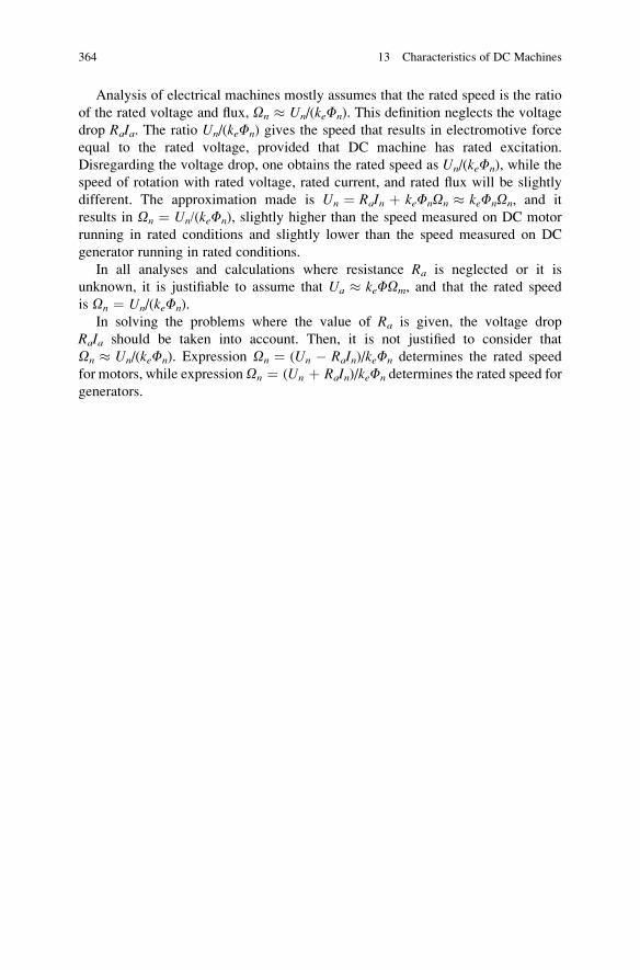
Analysis of electrical machines mostly assumes that the rated speed is the ratio
of the rated voltage and flux, On � Un/(keFn). This definition neglects the voltage
drop RaIa. The ratio Un/(keFn) gives the speed that results in electromotive force
equal to the rated voltage, provided that DC machine has rated excitation.
Disregarding the voltage drop, one obtains the rated speed as Un/(keFn), while the
speed of rotation with rated voltage, rated current, and rated flux will be slightly
different. The approximation made is Un ¼ RaIn þ keFnOn � keFnOn, and it
results in On ¼ Un/(keFn), slightly higher than the speed measured on DC motor
running in rated conditions and slightly lower than the speed measured on DC
generator running in rated conditions.
In all analyses and calculations where resistance Ra is neglected or it is
unknown, it is justifiable to assume that Ua � keFOm, and that the rated speed
is On ¼ Un/(keFn).
In solving the problems where the value of Ra is given, the voltage drop
RaIa should be taken into account. Then, it is not justified to consider that
On � Un/(keFn). Expression On ¼ (Un � RaIn)/keFn determines the rated speed
for motors, while expressionOn ¼ (Un þ RaIn)/keFn determines the rated speed for
generators.
364 13 Characteristics of DC Machines
Chapter 14
Induction Machines
The operating principles of induction machines and basic data concerning
constructions of their stator and rotor are presented in this chapter. This chapter
includes some basic information regarding construction of induction machines.
Discussed and described are the stator windings, the rotor short-circuited cage
winding, and slotted and laminated magnetic circuits of both stator and rotor.
Fundamentals on creating the revolving magnetic field are reinstated for the
three-phase stator winding. Basic operating principles of an induction machine
are illustrated on simplified machine with one short-circuited rotor turn. The torque
expression is developed and used to predict basic properties of mechanical charac-
teristic. For the purpose of studying the electrical and mechanical properties
of induction machines, corresponding mathematical model is developed in
Chap. 15 and used within the next chapters. Chapter 16 deals with the steady-
state operation, steady-state equivalent circuit and relevant parameters, mechanical
characteristics, losses, and power balance. Variable speed operation of induction
machines is discussed in Chap. 17, with analysis of constant frequency-supplied
induction machines and introduction and analysis of variable frequency-supplied
induction machines, fed from PWM-controlled three-phase inverters.
14.1 Construction and Operating Principles
Induction machines have stator comprising three-phase windings. Magnetic axes
of the three phases are spatially shifted by 2p/3. If the stator phase windings havesinusoidal currents of the same amplitude and the same angular frequency oe, and
at the same time their initial phases mutually differ by 2p/3, then the magnetic
field within the machine revolves, maintaining the same amplitude. The speed
of the field rotation is determined by the angular frequency oe of the source
voltage. When an induction machine is fed from a network of industrial frequency
f ¼ 50 Hz, the field rotates at the speed of 100p rad/s. The rotor of an induction
machine has a short-circuited cage winding. If the rotor revolves at the same
S.N. Vukosavic, Electrical Machines, Power Electronics and Power Systems,
DOI 10.1007/978-1-4614-0400-2_14, # Springer Science+Business Media New York 2013
365
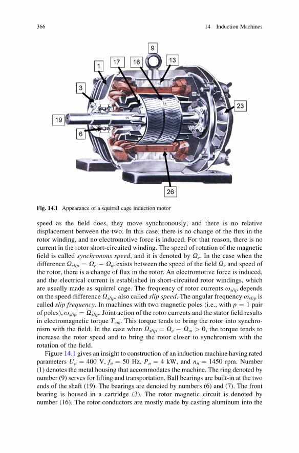
speed as the field does, they move synchronously, and there is no relative
displacement between the two. In this case, there is no change of the flux in the
rotor winding, and no electromotive force is induced. For that reason, there is no
current in the rotor short-circuited winding. The speed of rotation of the magnetic
field is called synchronous speed, and it is denoted by Oe. In the case when the
difference Oslip ¼ Oe � Om exists between the speed of the field Oe and speed of
the rotor, there is a change of flux in the rotor. An electromotive force is induced,
and the electrical current is established in short-circuited rotor windings, which
are usually made as squirrel cage. The frequency of rotor currents oslip depends
on the speed difference Oslip, also called slip speed. The angular frequency oslip is
called slip frequency. In machines with two magnetic poles (i.e., with p ¼ 1 pair
of poles), oslip ¼ Oslip. Joint action of the rotor currents and the stator field results
in electromagnetic torque Tem. This torque tends to bring the rotor into synchro-
nism with the field. In the case when Oslip ¼ Oe � Om > 0, the torque tends to
increase the rotor speed and to bring the rotor closer to synchronism with the
rotation of the field.
Figure 14.1 gives an insight to construction of an induction machine having rated
parameters Un ¼ 400 V, fn ¼ 50 Hz, Pn ¼ 4 kW, and nn ¼ 1450 rpm. Number
(1) denotes the metal housing that accommodates the machine. The ring denoted by
number (9) serves for lifting and transportation. Ball bearings are built-in at the two
ends of the shaft (19). The bearings are denoted by numbers (6) and (7). The front
bearing is housed in a cartridge (3). The rotor magnetic circuit is denoted by
number (16). The rotor conductors are mostly made by casting aluminum into the
Fig. 14.1 Appearance of a squirrel cage induction motor
366 14 Induction Machines
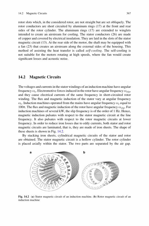
rotor slots which, in the considered rotor, are not straight but are set obliquely. The
rotor conductors are short circuited by aluminum rings (17) at the front and rear
sides of the rotor cylinder. The aluminum rings (17) are extended to winglets
intended to create an airstream for cooling. The stator conductors (26) are made
of copper and covered by electrical insulation. They are laid in the slots of the stator
magnetic circuit (13). At the rear side of the motor, the shaft may be equipped with
a fan (23) that creates an airstream along the external sides of the housing. This
method of assisting the heat transfer is called self-cooling. The self-cooling is
not suitable for the motors rotating at high speeds, where the fan would create
significant losses and acoustic noise.
14.2 Magnetic Circuits
The voltages and currents in the stator windings of an inductionmachine have angular
frequencyoe. Electromotive forces induced in the rotor have angular frequencyoslip,
and they cause electrical currents of the same frequency in short-circuited rotor
winding. The flux and magnetic induction of the stator vary at angular frequency
oe. Induction machines operated from the mains have angular frequencyoe equal to
100p. The flux and magnetic induction of the rotor have angular frequencyoslip. For
induction machines of several kW, the slip frequency is of the order of 1 Hz. Hence,
magnetic induction pulsates with respect to the stator magnetic circuit at the line
frequency. It also pulsates with respect to the rotor magnetic circuits at lower
frequency. In order to reduce iron losses due to eddy currents, both stator and rotor
magnetic circuits are laminated, that is, they are made of iron sheets. The shape of
these sheets is shown in Fig. 14.2.
By stacking iron sheets, cylindrical magnetic circuits of the stator and rotor
are obtained. The stator magnetic circuit is a hollow cylinder. The rotor cylinder
is placed axially within the stator. The two parts are separated by the air gap.
Fig. 14.2 (a) Stator magnetic circuit of an induction machine. (b) Rotor magnetic circuit of an
induction machine
14.2 Magnetic Circuits 367
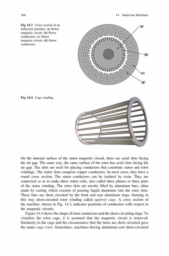
On the internal surface of the stator magnetic circuit, there are axial slots facing
the air gap. The same way, the outer surface of the rotor has axial slots facing the
air gap. The slots are used for placing conductors that constitute stator and rotor
windings. The stator slots comprise copper conductors. In most cases, they have a
round cross section. The stator conductors can be isolated by resin. They are
connected so as to make three stator coils, also called three phases or three parts
of the stator winding. The rotor slots are mostly filled by aluminum bars, often
made by casting which consists of pouring liquid aluminum into the rotor slots.
These bars are short circuited by the front and rear aluminum rings, forming in
this way short-circuited rotor winding called squirrel cage. A cross section of
the machine, shown in Fig. 14.3, indicates positions of conductors with respect to
the magnetic circuits.
Figure 14.4 shows the shape of rotor conductors and the short-circuiting rings. To
visualize the rotor cage, it is assumed that the magnetic circuit is removed.
Similarity to the cage and the circumstance that the turns are short circuited gave
the name cage rotor. Sometimes, machines having aluminum-cast short-circuited
Fig. 14.3 Cross section of an
induction machine. (a) Rotor
magnetic circuit. (b) Rotor
conductors. (c) Stator
magnetic circuit. (d) Stator
conductors
Fig. 14.4 Cage winding
368 14 Induction Machines
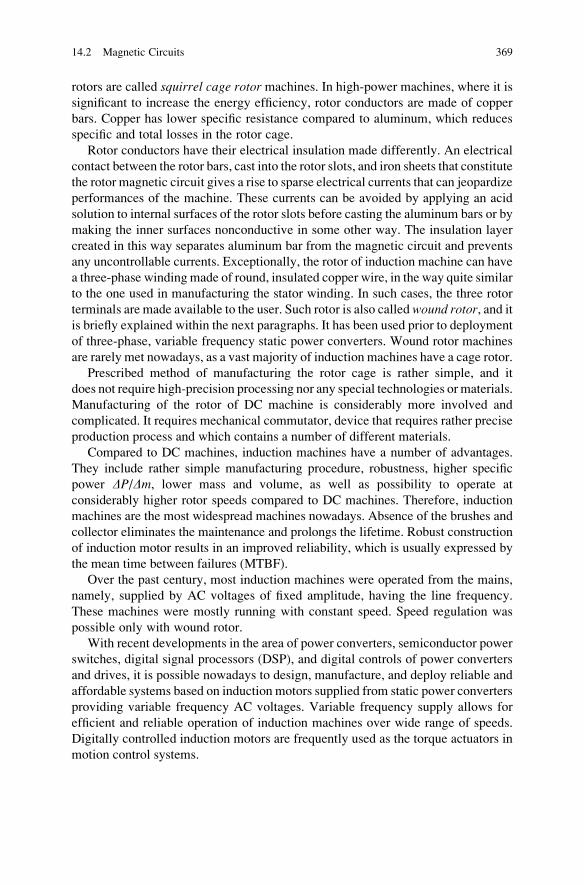
rotors are called squirrel cage rotor machines. In high-power machines, where it is
significant to increase the energy efficiency, rotor conductors are made of copper
bars. Copper has lower specific resistance compared to aluminum, which reduces
specific and total losses in the rotor cage.
Rotor conductors have their electrical insulation made differently. An electrical
contact between the rotor bars, cast into the rotor slots, and iron sheets that constitute
the rotor magnetic circuit gives a rise to sparse electrical currents that can jeopardize
performances of the machine. These currents can be avoided by applying an acid
solution to internal surfaces of the rotor slots before casting the aluminum bars or by
making the inner surfaces nonconductive in some other way. The insulation layer
created in this way separates aluminum bar from the magnetic circuit and prevents
any uncontrollable currents. Exceptionally, the rotor of induction machine can have
a three-phase winding made of round, insulated copper wire, in the way quite similar
to the one used in manufacturing the stator winding. In such cases, the three rotor
terminals are made available to the user. Such rotor is also calledwound rotor, and itis briefly explained within the next paragraphs. It has been used prior to deployment
of three-phase, variable frequency static power converters. Wound rotor machines
are rarely met nowadays, as a vast majority of induction machines have a cage rotor.
Prescribed method of manufacturing the rotor cage is rather simple, and it
does not require high-precision processing nor any special technologies or materials.
Manufacturing of the rotor of DC machine is considerably more involved and
complicated. It requires mechanical commutator, device that requires rather precise
production process and which contains a number of different materials.
Compared to DC machines, induction machines have a number of advantages.
They include rather simple manufacturing procedure, robustness, higher specific
power DP/Dm, lower mass and volume, as well as possibility to operate at
considerably higher rotor speeds compared to DC machines. Therefore, induction
machines are the most widespread machines nowadays. Absence of the brushes and
collector eliminates the maintenance and prolongs the lifetime. Robust construction
of induction motor results in an improved reliability, which is usually expressed by
the mean time between failures (MTBF).
Over the past century, most induction machines were operated from the mains,
namely, supplied by AC voltages of fixed amplitude, having the line frequency.
These machines were mostly running with constant speed. Speed regulation was
possible only with wound rotor.
With recent developments in the area of power converters, semiconductor power
switches, digital signal processors (DSP), and digital controls of power converters
and drives, it is possible nowadays to design, manufacture, and deploy reliable and
affordable systems based on induction motors supplied from static power converters
providing variable frequency AC voltages. Variable frequency supply allows for
efficient and reliable operation of induction machines over wide range of speeds.
Digitally controlled induction motors are frequently used as the torque actuators in
motion control systems.
14.2 Magnetic Circuits 369
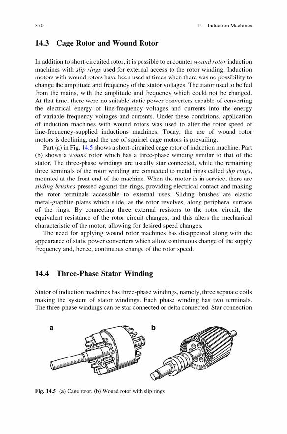
14.3 Cage Rotor and Wound Rotor
In addition to short-circuited rotor, it is possible to encounter wound rotor inductionmachines with slip rings used for external access to the rotor winding. Induction
motors with wound rotors have been used at times when there was no possibility to
change the amplitude and frequency of the stator voltages. The stator used to be fed
from the mains, with the amplitude and frequency which could not be changed.
At that time, there were no suitable static power converters capable of converting
the electrical energy of line-frequency voltages and currents into the energy
of variable frequency voltages and currents. Under these conditions, application
of induction machines with wound rotors was used to alter the rotor speed of
line-frequency-supplied inductions machines. Today, the use of wound rotor
motors is declining, and the use of squirrel cage motors is prevailing.
Part (a) in Fig. 14.5 shows a short-circuited cage rotor of induction machine. Part
(b) shows a wound rotor which has a three-phase winding similar to that of the
stator. The three-phase windings are usually star connected, while the remaining
three terminals of the rotor winding are connected to metal rings called slip rings,mounted at the front end of the machine. When the motor is in service, there are
sliding brushes pressed against the rings, providing electrical contact and making
the rotor terminals accessible to external uses. Sliding brushes are elastic
metal-graphite plates which slide, as the rotor revolves, along peripheral surface
of the rings. By connecting three external resistors to the rotor circuit, the
equivalent resistance of the rotor circuit changes, and this alters the mechanical
characteristic of the motor, allowing for desired speed changes.
The need for applying wound rotor machines has disappeared along with the
appearance of static power converters which allow continuous change of the supply
frequency and, hence, continuous change of the rotor speed.
14.4 Three-Phase Stator Winding
Stator of induction machines has three-phase windings, namely, three separate coils
making the system of stator windings. Each phase winding has two terminals.
The three-phase windings can be star connected or delta connected. Star connection
Fig. 14.5 (a) Cage rotor. (b) Wound rotor with slip rings
370 14 Induction Machines
is denoted by Y and delta connection by D. With star connection, one terminal of
each phase winding is connected to three-phase AC source, while the other phase
terminals are connected to a common node. This common node is called star point.With the star point having no other connections (floating), the sum of the
three-phase currents must be equal to zero at every instant, ia(t) + ib(t) + ic(t) ¼ 0.
Most star-connected stator windings have their star point floating. Exceptionally,
some large-power, high-voltage1 induction machines may have their star point
connected.2
In some cases, phases of the three-phase stator winding are connected to deltaconnection, wherein the three-phase windings are connected into triangle, restricting
the phase voltages by ua(t) + ub(t) + uc(t) ¼ 0. For the given power rating, delta
connection has lower current in stator conductors with respect to star connection.
Therefore, delta connection is advantageously used in electrical machines with
exceptionally low stator voltages, such as the motors in battery-fed traction drives,
where the stator current is very large.
There are advantages of star connection which make it more frequently used.3
Without the lack of generality, it is assumed throughout this book that the stator
phases are star connected.
Magnetic axes of the stator phase windings are spatially shifted by 2p/3, as shownin Fig. 14.6. Desired magnetic field within three-phase induction machines is
established by establishing the phase currents of the same amplitude Im and the
same angular frequencyoe. Their initial phases have to be shifted by 2p/3, the anglethat corresponds to the spatial shift between magnetic axes of the three phases. With
prescribed currents in the phase windings, magnetic field is established in magnetic
circuits and the air gap of the machine. The field revolves at angular speedOe ¼ oe.4
The phase currents of the same amplitude and frequency, and with the initial phase
1Voltages in excess to 1 kV are called high voltages. The termmedium voltage is also in use, and itrefers to lower end of high voltages and corresponds to voltages from 1 up to 10 kV. The upper
limit of medium voltages is not strictly defined. There are also terms very high voltages and
ultrahigh voltage, both lacking a clear definition.2 High-voltage induction machines have an increased insulation stress. Due to transient phenom-
ena, floating star point may have considerable overvoltages. In some cases, star point of high-
voltage machines is grounded by means of impedance connected between the star point and the
ground.3 The sum of the phase voltages of delta-connected phase windings is equal to zero, ua(t) +ub(t) + uc(t) ¼ 0. Practical AC machines have imperfect, nonsinusoidal electromotive forces that
include harmonics such as the third, which has the same initial phase in all the three-phase windings.
This is the property of all 3nth harmonic, also called triplian harmonics. Within the three phases of
the stator winding, the waveforms of a triplian harmonics have the same amplitude and phase.
Therefore, with star connection, triplian harmonics cannot produce any current due to ia(t) + ib(t) +ic(t) ¼ 0. On the other hand, delta connection provides the circular path for triplian harmonics of the
stator current. With delta connection, any distortion in electromotive forces that results triplian
harmonics contributes to circular currents which compromise the operation of induction machine by
increasing losses.4With induction machines having p > 1 pairs of magnetic poles, Oe ¼ oe/p. Machines with
multiple pairs of magnetic poles are explained further on.
14.4 Three-Phase Stator Winding 371
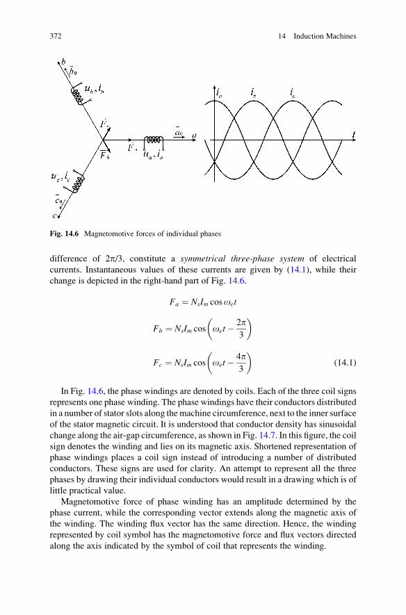
difference of 2p/3, constitute a symmetrical three-phase system of electrical
currents. Instantaneous values of these currents are given by (14.1), while their
change is depicted in the right-hand part of Fig. 14.6.
Fa ¼ NsIm cosoet
Fb ¼ NsIm cos oet� 2p3
� �
Fc ¼ NsIm cos oet� 4p3
� �(14.1)
In Fig. 14.6, the phase windings are denoted by coils. Each of the three coil signs
represents one phase winding. The phase windings have their conductors distributed
in a number of stator slots along themachine circumference, next to the inner surface
of the stator magnetic circuit. It is understood that conductor density has sinusoidal
change along the air-gap circumference, as shown in Fig. 14.7. In this figure, the coil
sign denotes the winding and lies on its magnetic axis. Shortened representation of
phase windings places a coil sign instead of introducing a number of distributed
conductors. These signs are used for clarity. An attempt to represent all the three
phases by drawing their individual conductors would result in a drawing which is of
little practical value.
Magnetomotive force of phase winding has an amplitude determined by the
phase current, while the corresponding vector extends along the magnetic axis of
the winding. The winding flux vector has the same direction. Hence, the winding
represented by coil symbol has the magnetomotive force and flux vectors directed
along the axis indicated by the symbol of coil that represents the winding.
Fig. 14.6 Magnetomotive forces of individual phases
372 14 Induction Machines
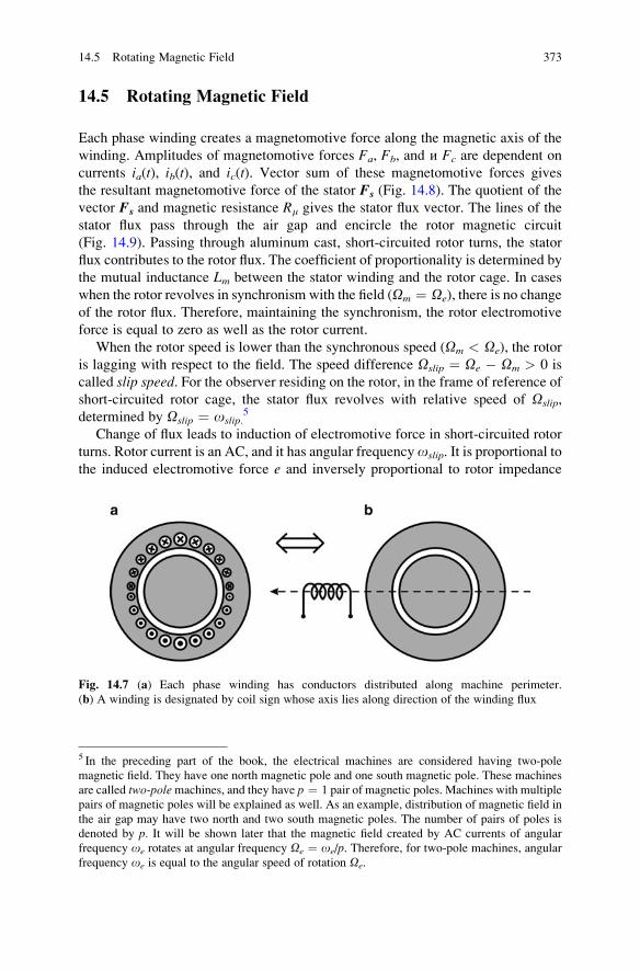
14.5 Rotating Magnetic Field
Each phase winding creates a magnetomotive force along the magnetic axis of the
winding. Amplitudes of magnetomotive forces Fa, Fb, and и Fc are dependent on
currents ia(t), ib(t), and ic(t). Vector sum of these magnetomotive forces gives
the resultant magnetomotive force of the stator Fs (Fig. 14.8). The quotient of the
vector Fs and magnetic resistance Rm gives the stator flux vector. The lines of the
stator flux pass through the air gap and encircle the rotor magnetic circuit
(Fig. 14.9). Passing through aluminum cast, short-circuited rotor turns, the stator
flux contributes to the rotor flux. The coefficient of proportionality is determined by
the mutual inductance Lm between the stator winding and the rotor cage. In cases
when the rotor revolves in synchronism with the field (Om ¼ Oe), there is no change
of the rotor flux. Therefore, maintaining the synchronism, the rotor electromotive
force is equal to zero as well as the rotor current.
When the rotor speed is lower than the synchronous speed (Om < Oe), the rotor
is lagging with respect to the field. The speed difference Oslip ¼ Oe � Om > 0 is
called slip speed. For the observer residing on the rotor, in the frame of reference of
short-circuited rotor cage, the stator flux revolves with relative speed of Oslip,
determined by Oslip ¼ oslip.5
Change of flux leads to induction of electromotive force in short-circuited rotor
turns. Rotor current is an AC, and it has angular frequencyoslip. It is proportional to
the induced electromotive force e and inversely proportional to rotor impedance
Fig. 14.7 (a) Each phase winding has conductors distributed along machine perimeter.
(b) A winding is designated by coil sign whose axis lies along direction of the winding flux
5 In the preceding part of the book, the electrical machines are considered having two-pole
magnetic field. They have one north magnetic pole and one south magnetic pole. These machines
are called two-polemachines, and they have p ¼ 1 pair of magnetic poles. Machines with multiple
pairs of magnetic poles will be explained as well. As an example, distribution of magnetic field in
the air gap may have two north and two south magnetic poles. The number of pairs of poles is
denoted by p. It will be shown later that the magnetic field created by AC currents of angular
frequency oe rotates at angular frequency Oe ¼ oe/p. Therefore, for two-pole machines, angular
frequency oe is equal to the angular speed of rotation Oe.
14.5 Rotating Magnetic Field 373
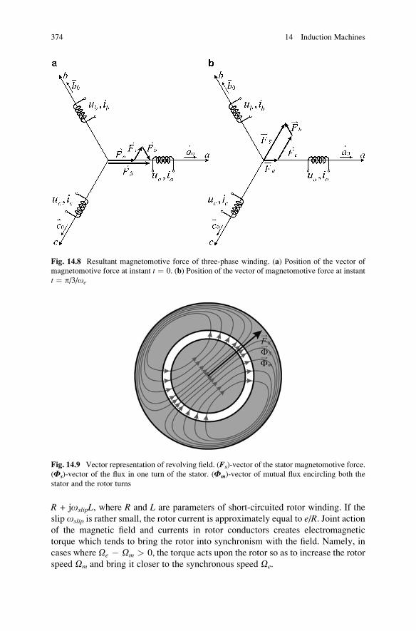
R + joslipL, where R and L are parameters of short-circuited rotor winding. If the
slip oslip is rather small, the rotor current is approximately equal to e/R. Joint actionof the magnetic field and currents in rotor conductors creates electromagnetic
torque which tends to bring the rotor into synchronism with the field. Namely, in
cases where Oe � Om > 0, the torque acts upon the rotor so as to increase the rotor
speed Om and bring it closer to the synchronous speed Oe.
Fig. 14.8 Resultant magnetomotive force of three-phase winding. (a) Position of the vector of
magnetomotive force at instant t ¼ 0. (b) Position of the vector of magnetomotive force at instant
t ¼ p/3/oe
Fig. 14.9 Vector representation of revolving field. (Fs)-vector of the stator magnetomotive force.
(Fs)-vector of the flux in one turn of the stator. (Fm)-vector of mutual flux encircling both the
stator and the rotor turns
374 14 Induction Machines
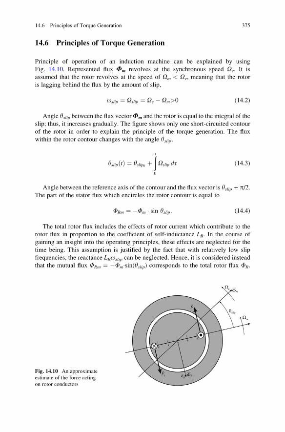
14.6 Principles of Torque Generation
Principle of operation of an induction machine can be explained by using
Fig. 14.10. Represented flux Fm revolves at the synchronous speed Oe. It is
assumed that the rotor revolves at the speed of Om < Oe, meaning that the rotor
is lagging behind the flux by the amount of slip,
oslip ¼ Oslip ¼ Oe � Om>0 (14.2)
Angle yslip between the flux vectorFm and the rotor is equal to the integral of the
slip; thus, it increases gradually. The figure shows only one short-circuited contour
of the rotor in order to explain the principle of the torque generation. The flux
within the rotor contour changes with the angle yslip,
yslipðtÞ ¼ yslip0 þðt
0
Oslip dt (14.3)
Angle between the reference axis of the contour and the flux vector is yslip + p/2.The part of the stator flux which encircles the rotor contour is equal to
FRm ¼ �Fm � sin yslip: (14.4)
The total rotor flux includes the effects of rotor current which contribute to the
rotor flux in proportion to the coefficient of self-inductance LR. In the course of
gaining an insight into the operating principles, these effects are neglected for the
time being. This assumption is justified by the fact that with relatively low slip
frequencies, the reactance LRoslip can be neglected. Hence, it is considered instead
that the mutual flux FRm ¼ �Fm�sin(yslip) corresponds to the total rotor flux FR.
Fig. 14.10 An approximate
estimate of the force acting
on rotor conductors
14.6 Principles of Torque Generation 375
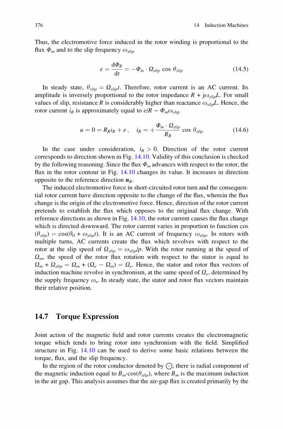
Thus, the electromotive force induced in the rotor winding is proportional to the
flux Fm and to the slip frequency oslip
e ¼ dFR
dt¼ �Fm � Oslip cos yslip (14.5)
In steady state, yslip ¼ Oslipt. Therefore, rotor current is an AC current. Its
amplitude is inversely proportional to the rotor impedance R + joslipL. For small
values of slip, resistance R is considerably higher than reactance oslipL. Hence, therotor current iR is approximately equal to e/R ~ Fmoslip
u ¼ 0 ¼ RRiR þ e ; iR ¼ þFm � Oslip
RRcos yslip (14.6)
In the case under consideration, iR > 0. Direction of the rotor current
corresponds to direction shown in Fig. 14.10. Validity of this conclusion is checked
by the following reasoning. Since the fluxFm advances with respect to the rotor, the
flux in the rotor contour in Fig. 14.10 changes its value. It increases in direction
opposite to the reference direction nR.The induced electromotive force in short-circuited rotor turn and the consequen-
tial rotor current have direction opposite to the change of the flux, wherein the flux
change is the origin of the electromotive force. Hence, direction of the rotor current
pretends to establish the flux which opposes to the original flux change. With
reference directions as shown in Fig. 14.10, the rotor current causes the flux change
which is directed downward. The rotor current varies in proportion to function cos
(yslip) ¼ cos(y0 + oslipt). It is an AC current of frequency oslip. In rotors with
multiple turns, AC currents create the flux which revolves with respect to the
rotor at the slip speed of Oslip ¼ oslip/p. With the rotor running at the speed of
Om, the speed of the rotor flux rotation with respect to the stator is equal to
Om + Oslip ¼ Om + (Oe � Om) ¼ Oe. Hence, the stator and rotor flux vectors of
induction machine revolve in synchronism, at the same speed of Oe, determined by
the supply frequency oe. In steady state, the stator and rotor flux vectors maintain
their relative position.
14.7 Torque Expression
Joint action of the magnetic field and rotor currents creates the electromagnetic
torque which tends to bring rotor into synchronism with the field. Simplified
structure in Fig. 14.10 can be used to derive some basic relations between the
torque, flux, and the slip frequency.
In the region of the rotor conductor denoted byJ
, there is radial component of
the magnetic induction equal to Bm�cos(yslip), where Bm is the maximum induction
in the air gap. This analysis assumes that the air-gap flux is created primarily by the
376 14 Induction Machines
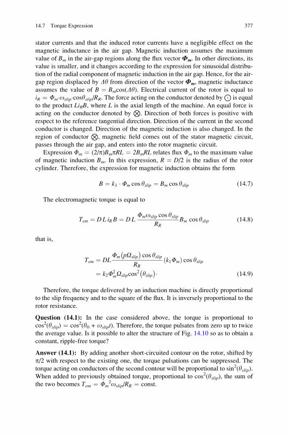
stator currents and that the induced rotor currents have a negligible effect on the
magnetic inductance in the air gap. Magnetic induction assumes the maximum
value of Bm in the air-gap regions along the flux vector Fm. In other directions, its
value is smaller, and it changes according to the expression for sinusoidal distribu-
tion of the radial component of magnetic induction in the air gap. Hence, for the air-
gap region displaced by Dy from direction of the vector Fm, magnetic inductance
assumes the value of B ¼ Bmcos(Dy). Electrical current of the rotor is equal to
iR ¼ Fm�oslip�cosyslip/RR. The force acting on the conductor denoted byJ
is equal
to the product LiRB, where L is the axial length of the machine. An equal force is
acting on the conductor denoted byN
. Direction of both forces is positive with
respect to the reference tangential direction. Direction of the current in the second
conductor is changed. Direction of the magnetic induction is also changed. In the
region of conductorN
, magnetic field comes out of the stator magnetic circuit,
passes through the air gap, and enters into the rotor magnetic circuit.
Expression Fm ¼ (2/p)BmpRL ¼ 2BmRL relates flux Fm to the maximum value
of magnetic induction Bm. In this expression, R ¼ D/2 is the radius of the rotor
cylinder. Therefore, the expression for magnetic induction obtains the form
B ¼ k1 � Fm cos yslip ¼ Bm cos yslip (14.7)
The electromagnetic torque is equal to
Tem ¼ DL iR B ¼ DLFmoslip cos yslip
RRBm cos yslip (14.8)
that is,
Tem ¼ DLFm pOslip
� �cos yslip
RRk1Fmð Þ cos yslip
¼ k2F2mOslipcos
2 yslip� �� (14.9)
Therefore, the torque delivered by an induction machine is directly proportional
to the slip frequency and to the square of the flux. It is inversely proportional to the
rotor resistance.
Question (14.1): In the case considered above, the torque is proportional to
cos2(yslip) ¼ cos2(y0 + oslipt). Therefore, the torque pulsates from zero up to twice
the average value. Is it possible to alter the structure of Fig. 14.10 so as to obtain a
constant, ripple-free torque?
Answer (14.1): By adding another short-circuited contour on the rotor, shifted by
p/2 with respect to the existing one, the torque pulsations can be suppressed. The
torque acting on conductors of the second contour will be proportional to sin2(yslip).When added to previously obtained torque, proportional to cos2(yslip), the sum of
the two becomes Tem ¼ Fm2oslip/RR ¼ const.
14.7 Torque Expression 377
Chapter 15
Modeling of Induction Machines
This chapter introduces and explains mathematical model of induction machines.
This model represents transient and steady-state behavior in electrical and mechan-
ical subsystems of the machine. Analysis and discussion introduces and explains
Clarke and Park coordinate transforms. The model includes differential equations
that express the voltage balance in stator and rotor windings, inductance matrix
which relates flux linkages and currents, Newton differential equation of motion,
expression for the air-gap power, and expression for the electromagnetic torque.
The model development process starts with replacing the three-phase machine with
two-phase equivalent. Namely, the three-phase voltages, currents, and flux linkages
are transformed in two-phase variables by appropriate transformation matrix which
implements 3F/2F transform, also called Clarke coordinate transform. Two-phase
model is formulated in stationary coordinate frame. The drawbacks and difficulties
in using this model are the rationale for introducing and applying Park coordinate
transform, which results in the machine model in synchronous dq coordinate frame.
Necessary techniques and procedures of applying and using coordinate transforms
are explained in detail, including representation of machine vectors by complex
numbers. The operable model of induction machines is obtained in dq coordinate
frame which revolves synchronously with the stator field. The merits and practical
uses of the model in dq frame are explained at the end of the chapter.
15.1 Modeling Steady State and Transient Phenomena
The work with induction machines requires a sound knowledge of their behavior
and principal characteristics. From the electrical access point, it is of interest to find
relations between steady-state voltage and currents, so as to obtain an equivalent
circuit of the machine, representing the steady-state operation. At the same time, it
is important to study the torque–speed relations at the mechanical access of the
machine.
S.N. Vukosavic, Electrical Machines, Power Electronics and Power Systems,
DOI 10.1007/978-1-4614-0400-2_15, # Springer Science+Business Media New York 2013
379
Analysis of induction machines at steady state is based on mechanicalcharacteristics and steady-state equivalent circuit. Mechanical characteristic of
an induction machine gives relation between steady-state values of the electromag-
netic torque and the rotor speed. The mechanical characteristic is dependent on the
frequency and amplitude of the stator voltage. Therefore, any change in stator
voltage will affect the mechanical characteristic. At steady state, the voltages and
currents are sinusoidal quantities of constant amplitude and frequency. For that
reason, they can be represented by appropriate phasors.1 Relations between
voltages and currents can be presented by equivalent circuit. A steady-state equiv-
alent circuit is a network consisting of resistances and reactances which serves for
calculation of phasors of the stator and rotor currents in conditions with known
supply conditions and specified rotor speed.
Working on problems of supplying and controlling induction machines
requires a good knowledge of the dynamic model. This model comprises differen-
tial equations and algebraic expressions relating the machine variables and
parameters during transient processes and also in the steady state. Relation between
the voltages and currents during transients is given by differential equations
describing the voltage equilibrium in the windings, also called voltage balanceequations. The voltage balance equations describe the electrical subsystem of
induction machine. The mechanical subsystem is described by Newton differential
equation of motion. The set of differential equations and expressions describing
behavior of the machine is called mathematical model or dynamic model.In further considerations, the analyses of electrical and mechanical subsystems
of induction machines are presented and explained, resulting in dynamic model.
This model includes transforms of the state coordinates, also called coordinatetransforms. They facilitate the analysis of transient processes in both synchronous
and induction machines. Dynamic model is usually mostly used for transient
analysis and for solving control problems, but it can also be used to resolve steady
states. Starting from dynamic model, one can obtain the steady-state relations;
mechanical characteristics; relations between voltages, currents, fluxes, torques,
and speed in the steady state; as well as the steady-state equivalent circuit.
The readers with no interest in transient processes in induction machines and
with no need to deal with problems of supply and control do not have to study
dynamic model of induction machine. Such readers could skip entire Chap. 15
which develops mathematical model and deals with transient processes. The
steady-state equivalent circuit can be also determined by using analogy with a
transformer, as shown in Sect. 16.6. The analyses of steady-state equivalent circuits
and the study of mechanical characteristics of induction machines can be continued
in Chap. 16.
1 Phasor is a complex number which represents a sinusoidal AC voltage or current. The absolute
value of phasor corresponds to the amplitude, while the phasor argument determines the initial
phase of considered voltages and currents. Phasors can be used to represent other quantities that
have sinusoidal change in steady state, such as the magnetomotive forces and fluxes.
380 15 Modeling of Induction Machines
15.2 The Structure of Mathematical Model
Within the introductory chapters, it is shown that the dynamic model of electrical
machines comprises four basic parts. These are:
1. N differential equations of voltage equilibrium
2. Inductance matrix
3. Expression for the torque
4. Newton equation
Differential equations of voltage balance are given by expression
u ¼ R � iþ dCdt
: (15.1)
Relation between the fluxes and currents is given by nonstationary inductance
matrix
C ¼ L ymð Þ � i: (15.2)
The electromagnetic torque is determined by equation
Tem ¼ 1
2iT
dL
dymi ¼ 1
2
XNk¼1
XNj¼1
ikijdLjkdym
� �: (15.3)
Transient phenomena in mechanical subsystem are determined by Newton
differential equation of motion
JdOm
dt¼ Tem � Tm � kFOm: (15.4)
The four equations given above define general model applicable to any rotating
electrical machine. The model is derived assuming four basic approximations:
1. The effects of distributed parameters are neglected.
2. The energy of electrical field is neglected along with parasitic capacitances.
3. The iron losses are neglected.
4. Magnetic saturation is neglected along with nonlinear B(H) characteristic of
ferromagnetic materials.
In the case when a machine has N windings, expression (15.1) contains Ndifferential equations of voltage balance, expression (15.2) provides relation
between the winding currents and their fluxes, expression (15.3) gives the electro-
magnetic torque, and expression (15.4) is in fact Newton differential equation
describing variation of the rotor speed. Therefore, in the presented model, there
are N þ 1 differential equations and the same number of state variables.
15.2 The Structure of Mathematical Model 381
15.3 Three-Phase and Two-Phase Machines
Most induction machines have a three-phase stator winding. Stator AC currents
create the vector of magnetomotive force FS ¼ Fa þ Fb þ Fc. This vector has a
radial direction within the machine, and it does not have any axial component.
Therefore, it resides in the plane defined by radial and tangential unit vectors of
cylindrical coordinate frame. The same plane can be represented by rectangular
coordinate system of two orthogonal axes, hereafter denoted by a and b. In order torepresent the vector in the a–b coordinate system, directions of axes a and b are
defined by their corresponding unit vectors a0 and b0.
While the machine has three-phase windings, spatially displaced by 2p/3,relevant vector will be displayed in a–b coordinate system. Therefore, there is a
need to express the orientation of the magnetic axes of individual phases in terms of
unit vectors a0 and b0:
~a0 ¼~a0;
~b0 ¼ �~a02þ
ffiffiffi3
p
2~b0;
~c0 ¼ �~a02�
ffiffiffi3
p
2~b0: (15.5)
With symmetrical set of three-phase voltages, the stator currents can be
expressed as
ia ¼ Im cosoet;
ib ¼ Im cosðoet� 2p=3Þ;ic ¼ Im cosðoet� 4p=3Þ; (15.6)
and they result in the following magnetomotive forces:
~Fa ¼ Nia~a0;
~Fb ¼ Nib � 1
2~a0 þ
ffiffiffi3
p
2~b0
� �;
~Fc ¼ Nic � 1
2~a0 �
ffiffiffi3
p
2~b0
� �: (15.7)
The sum of the three magnetomotive forces results in
~Fs ¼ ~Fa þ ~Fb þ ~Fc ¼ N ~a0 ia � ib2� ic
2
� �þ~b0
ffiffiffi3
p
2ib � icð Þ
� �;
~Fs ¼ 3
2NIm ~a0 cosoetþ~b0 sinoet
h i; (15.8)
382 15 Modeling of Induction Machines
the vector which revolves at the speed Oe ¼ oe and maintains the amplitude
FSm ¼ 3/2 NIm. Modeling three-phase winding encounters certain difficulties.
One of them is the fact that the phase currents are not independent variables.
They are restrained by relation ia þ ib þ ic ¼ 0, which comes from the circum-
stance that the windings are star connected. For delta connection, this problem has
different nature. Namely, the sum of the phase voltages of delta-connected winding
is equal to zero. Considering star-connected winding, conclusion is drawn that only
two out of three stator currents are independent variables. Therefore, in all differ-
ential equations, the current ic has to be replaced by (�ia�ib), making the equations
clumsy and difficult to work with. In addition, angular displacement between the
magnetic axis of the phase windings is 2p/3, resulting in nonzero values of mutual
inductances. An increased number of nonzero elements in the inductance matrix
increases the number of factors in voltage balance equations, making them more
involved and less intuitive. On the other hand, hypothetical two-phase machine can
be envisaged with only two currents and zero mutual inductance. The mathematical
model of an induction machine is more simple if considered machine has two-phase
windings on the stator, one of them oriented along unit vector a0 and the other
oriented along unit vector b0. The stator winding has only two electrical currents, iaand ib, and they are independent. Due to orthogonal magnetic axes of the windings,
their mutual inductance is zero, simplifying a great deal the voltage balance
equations.
In a two-phase machine with stator windings oriented along unit vectors a0 and
b0, the mathematical model becomes more usable because the winding currents
correspond to projections of the magnetomotive force vector on the axes a and b.Namely, the magnetomotive force component along the axis a is Fa ¼ Nia, whichis also projection of the vector FS on axis a. The magnetomotive force component
along the axis b is Fb ¼ Nib, equal to projection of the vector FS on axis b. Thesame conclusions can be derived for the flux vector. The flux in the phase winding ais equal to the projection of the flux vector FS on the axis a. Correspondencebetween the phase quantities and projections of relevant vectors on axes a and bfacilitates understanding and using the two-phase model.
One and the same magnetomotive force can be obtained with both three-phase
and the two-phase windings. The three-phase system of phase windings of Fig. 15.1
can be replaced by the two-phase system of phase windings, given in Fig. 15.2.
On the basis of (15.8) and assuming that the number of turns is unchanged
(Nabc ¼ Nab), the stator magnetomotive force vector FS retains the same orienta-
tion and amplitude provided that the electrical currents in the two-phase system are
ias ¼ ia � ib2� ic
2¼ 3
2ia ¼ 3
2Im cosoet
ibs ¼ffiffiffi3
p
2ib � icð Þ ¼ 3
2Im sinoet: (15.9)
15.3 Three-Phase and Two-Phase Machines 383
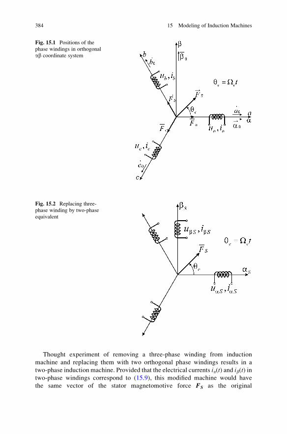
Thought experiment of removing a three-phase winding from induction
machine and replacing them with two orthogonal phase windings results in a
two-phase induction machine. Provided that the electrical currents ia(t) and ib(t) intwo-phase windings correspond to (15.9), this modified machine would have
the same vector of the stator magnetomotive force FS as the original
Fig. 15.1 Positions of the
phase windings in orthogonal
ab coordinate system
Fig. 15.2 Replacing three-
phase winding by two-phase
equivalent
384 15 Modeling of Induction Machines
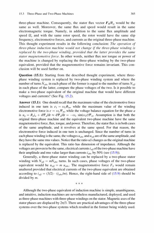
three-phase machine. Consequently, the stator flux vector FS/Rm would be the
same as well. Moreover, the same flux and speed would result in the same
electromagnetic torque. Namely, in addition to the same flux amplitude and
speed Oe and with the same rotor speed, the rotor would have the same slip
frequency, electromotive forces, and currents as the original three-phase machine.
This thought experiment results in the following conclusion: The operation ofthree-phase induction machine would not change if the three-phase winding isreplaced by the two-phase winding, provided that the latter provides the samestator magnetomotive force. In other words, neither flux nor torque or power of
the machine is changed by replacing the three-phase winding by the two-phase
equivalent, provided that the magnetomotive force remains invariant. This con-
clusion will be used further on.
Question (15.1): Starting from the described thought experiment, where three-
phase winding system is replaced by two-phase winding system and where the
number of turns Nabc in each phase of the former is equal to the number of turns Nab
in each phase of the latter, compare the phase voltages of the two. Is it possible to
make a two-phase equivalent of the original machine that would have different
voltages and currents? (See Fig. 15.2).
Answer (15.1): One should recall that the maximum value of the electromotive force
induced in one turn is e1 ¼ oeFm, while the maximum value of the winding
electromotive force is e ¼ oeCm, while the voltage balance equation for the phase ais ua ¼ Raia þ dCa/dt � dCa/dt ¼ �oe sin(oet)Cm. Assumption is that both the
original three-phase machine and the equivalent two-phase machine have the same
magnetomotive force, flux, torque, and power. Therefore, the stator flux is in both cases
of the same amplitude, and it revolves at the same speed. For that reason, the
electromotive force induced in one turn is unchanged. Since the number of turns in
eachphasewinding is the same, the voltagesuabc anduab are of the same amplitude, and
they have the same rms values. Notice that the ratio u/i changes as the original machine
is replaced by the equivalent. This ratio has dimension of impedance. Although the
voltages are proven to be the same, electrical currents iab of the two-phasemachine have
their amplitude and rms value larger than currents iabc by 50% (see (15.9)).
Generally, a three-phase stator winding can be replaced by a two-phase stator
winding with Nab ¼ mNabc turns. In such cases, phase voltages of the two-phase
equivalent would be uab ¼ m uabc. The magnetomotive force FS would remain
unaltered provided that electrical currents of the two-phase equivalent are obtained
according to iab ¼ (3/2) � (iabc/m). Hence, the right-hand side of (15.9) should be
divided by m.
* * *
Although the two-phase equivalent of induction machine is simple, unambiguous,
and intuitive, induction machines are nevertheless manufactured, deployed, and used
as three-phasemachines with three-phase windings on the stator. Magnetic axes of the
stator phases are displaced by 2p/3. There are practical advantages of the three-phasesystems over the two-phase systems which resulted in the former being widely used.
15.3 Three-Phase and Two-Phase Machines 385
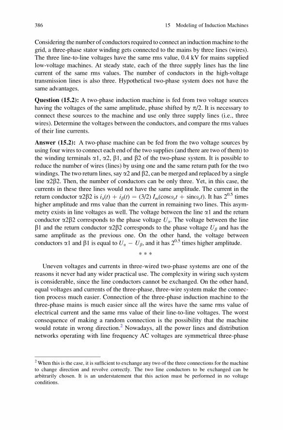
Considering the number of conductors required to connect an inductionmachine to the
grid, a three-phase stator winding gets connected to the mains by three lines (wires).
The three line-to-line voltages have the same rms value, 0.4 kV for mains supplied
low-voltage machines. At steady state, each of the three supply lines has the line
current of the same rms values. The number of conductors in the high-voltage
transmission lines is also three. Hypothetical two-phase system does not have the
same advantages.
Question (15.2): A two-phase induction machine is fed from two voltage sources
having the voltages of the same amplitude, phase shifted by p/2. It is necessary to
connect these sources to the machine and use only three supply lines (i.e., three
wires). Determine the voltages between the conductors, and compare the rms values
of their line currents.
Answer (15.2): A two-phase machine can be fed from the two voltage sources by
using four wires to connect each end of the two supplies (and there are two of them) to
the winding terminals a1, a2, b1, and b2 of the two-phase system. It is possible to
reduce the number of wires (lines) by using one and the same return path for the two
windings. The two return lines, say a2 and b2, can bemerged and replaced by a single
line a2b2. Then, the number of conductors can be only three. Yet, in this case, the
currents in these three lines would not have the same amplitude. The current in the
return conductor a2b2 is ia(t) þ ib(t) ¼ (3/2) Im(cosoet þ sinoet). It has 20.5 times
higher amplitude and rms value than the current in remaining two lines. This asym-
metry exists in line voltages as well. The voltage between the line a1 and the return
conductor a2b2 corresponds to the phase voltage Ua. The voltage between the line
b1 and the return conductor a2b2 corresponds to the phase voltage Ub and has the
same amplitude as the previous one. On the other hand, the voltage between
conductors a1 and b1 is equal to Ua � Ub, and it has 20.5 times higher amplitude.
* * *
Uneven voltages and currents in three-wired two-phase systems are one of the
reasons it never had any wider practical use. The complexity in wiring such system
is considerable, since the line conductors cannot be exchanged. On the other hand,
equal voltages and currents of the three-phase, three-wire system make the connec-
tion process much easier. Connection of the three-phase induction machine to the
three-phase mains is much easier since all the wires have the same rms value of
electrical current and the same rms value of their line-to-line voltages. The worst
consequence of making a random connection is the possibility that the machine
would rotate in wrong direction.2 Nowadays, all the power lines and distribution
networks operating with line frequency AC voltages are symmetrical three-phase
2When this is the case, it is sufficient to exchange any two of the three connections for the machine
to change direction and revolve correctly. The two line conductors to be exchanged can be
arbitrarily chosen. It is an understatement that this action must be performed in no voltage
conditions.
386 15 Modeling of Induction Machines
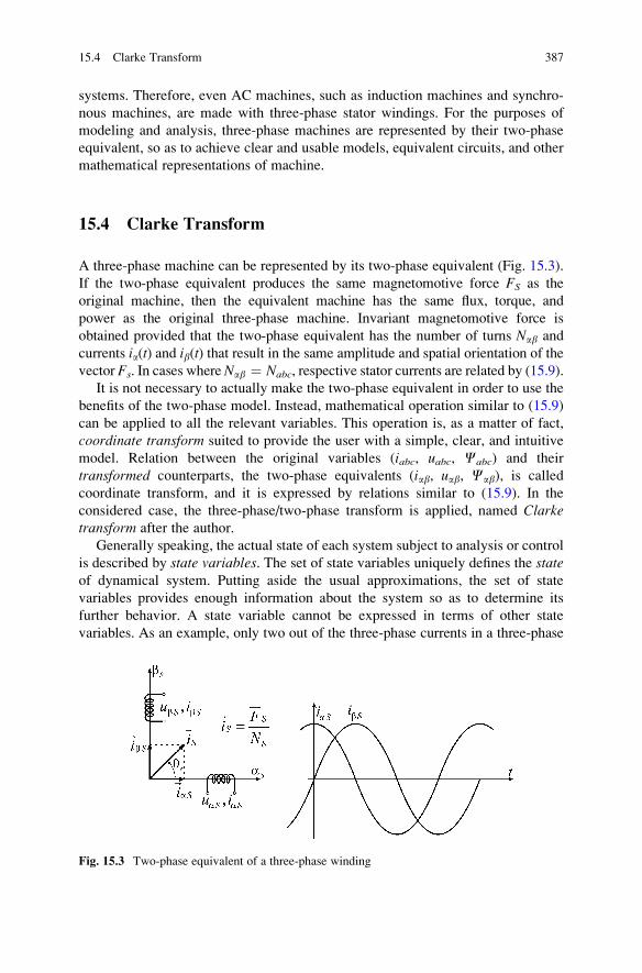
systems. Therefore, even AC machines, such as induction machines and synchro-
nous machines, are made with three-phase stator windings. For the purposes of
modeling and analysis, three-phase machines are represented by their two-phase
equivalent, so as to achieve clear and usable models, equivalent circuits, and other
mathematical representations of machine.
15.4 Clarke Transform
A three-phase machine can be represented by its two-phase equivalent (Fig. 15.3).
If the two-phase equivalent produces the same magnetomotive force FS as the
original machine, then the equivalent machine has the same flux, torque, and
power as the original three-phase machine. Invariant magnetomotive force is
obtained provided that the two-phase equivalent has the number of turns Nab and
currents ia(t) and ib(t) that result in the same amplitude and spatial orientation of the
vector Fs. In cases where Nab ¼ Nabc, respective stator currents are related by (15.9).
It is not necessary to actually make the two-phase equivalent in order to use the
benefits of the two-phase model. Instead, mathematical operation similar to (15.9)
can be applied to all the relevant variables. This operation is, as a matter of fact,
coordinate transform suited to provide the user with a simple, clear, and intuitive
model. Relation between the original variables (iabc, uabc, Cabc) and their
transformed counterparts, the two-phase equivalents (iab, uab, Cab), is called
coordinate transform, and it is expressed by relations similar to (15.9). In the
considered case, the three-phase/two-phase transform is applied, named Clarketransform after the author.
Generally speaking, the actual state of each system subject to analysis or control
is described by state variables. The set of state variables uniquely defines the stateof dynamical system. Putting aside the usual approximations, the set of state
variables provides enough information about the system so as to determine its
further behavior. A state variable cannot be expressed in terms of other state
variables. As an example, only two out of the three-phase currents in a three-phase
Fig. 15.3 Two-phase equivalent of a three-phase winding
15.4 Clarke Transform 387
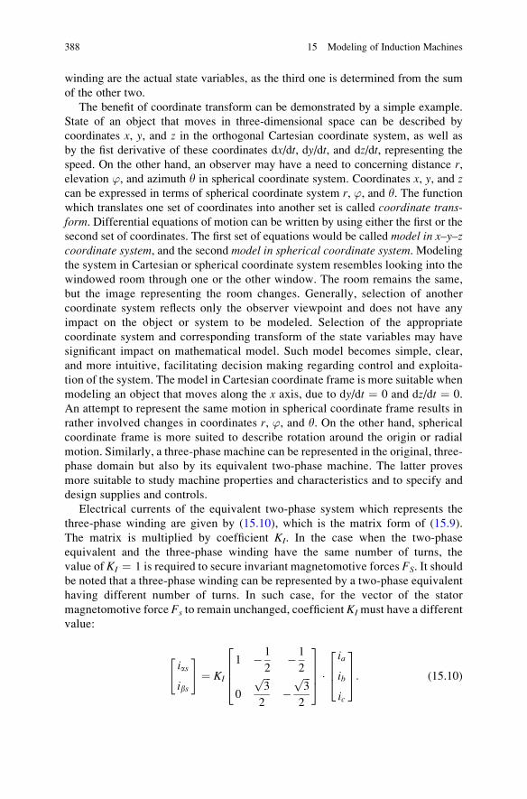
winding are the actual state variables, as the third one is determined from the sum
of the other two.
The benefit of coordinate transform can be demonstrated by a simple example.
State of an object that moves in three-dimensional space can be described by
coordinates x, y, and z in the orthogonal Cartesian coordinate system, as well as
by the fist derivative of these coordinates dx/dt, dy/dt, and dz/dt, representing the
speed. On the other hand, an observer may have a need to concerning distance r,elevation ’, and azimuth y in spherical coordinate system. Coordinates x, y, and zcan be expressed in terms of spherical coordinate system r, ’, and y. The functionwhich translates one set of coordinates into another set is called coordinate trans-form. Differential equations of motion can be written by using either the first or the
second set of coordinates. The first set of equations would be called model in x–y–zcoordinate system, and the second model in spherical coordinate system. Modeling
the system in Cartesian or spherical coordinate system resembles looking into the
windowed room through one or the other window. The room remains the same,
but the image representing the room changes. Generally, selection of another
coordinate system reflects only the observer viewpoint and does not have any
impact on the object or system to be modeled. Selection of the appropriate
coordinate system and corresponding transform of the state variables may have
significant impact on mathematical model. Such model becomes simple, clear,
and more intuitive, facilitating decision making regarding control and exploita-
tion of the system. The model in Cartesian coordinate frame is more suitable when
modeling an object that moves along the x axis, due to dy/dt ¼ 0 and dz/dt ¼ 0.
An attempt to represent the same motion in spherical coordinate frame results in
rather involved changes in coordinates r, ’, and y. On the other hand, spherical
coordinate frame is more suited to describe rotation around the origin or radial
motion. Similarly, a three-phase machine can be represented in the original, three-
phase domain but also by its equivalent two-phase machine. The latter proves
more suitable to study machine properties and characteristics and to specify and
design supplies and controls.
Electrical currents of the equivalent two-phase system which represents the
three-phase winding are given by (15.10), which is the matrix form of (15.9).
The matrix is multiplied by coefficient KI. In the case when the two-phase
equivalent and the three-phase winding have the same number of turns, the
value of KI ¼ 1 is required to secure invariant magnetomotive forces FS. It should
be noted that a three-phase winding can be represented by a two-phase equivalent
having different number of turns. In such case, for the vector of the stator
magnetomotive force Fs to remain unchanged, coefficient KImust have a different
value:
ias
ibs
" #¼ KI
1 � 1
2� 1
2
0
ffiffiffi3
p
2�
ffiffiffi3
p
2
2664
3775 �
ia
ib
ic
264
375: (15.10)
388 15 Modeling of Induction Machines
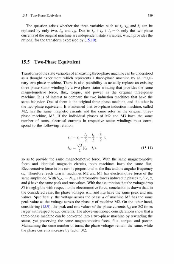
The question arises whether the three variables such as ia, ib, and ic can be
replaced by only two, ias and ibs. Due to ia þ ib þ ic ¼ 0, only the two-phase
currents of the original machine are independent state variables, which provides the
rational for the transform expressed by (15.10).
15.5 Two-Phase Equivalent
Transform of the state variables of an existing three-phase machine can be understood
as a thought experiment which represents a three-phase machine by an imagi-
nary two-phase machine. There is also possibility to actually replace an existing
three-phase stator winding by a two-phase stator winding that provides the same
magnetomotive force, flux, torque, and power as the original three-phase
machine. It is of interest to compare the two induction machines that have the
same behavior. One of them is the original three-phase machine, and the other is
the two-phase equivalent. It is assumed that two-phase induction machine, called
M2, has the same magnetic circuits and the same rotor as the original three-
phase machine, M3. If the individual phases of M2 and M3 have the same
number of turns, electrical currents in respective stator windings must corre-
spond to the following relation:
ias ¼ ia � ib2� ic
2¼ 3
2ia
ibs ¼ffiffiffi3
p
2ib � icð Þ: (15.11)
so as to provide the same magnetomotive force. With the same magnetomotive
force and identical magnetic circuits, both machines have the same flux.
Electromotive force in one turn is proportional to the flux and the angular frequency
oe. Therefore, each turn in machines M2 and M3 has electromotive force of the
same amplitude. With Nabc ¼ Nab, electromotive forces induced in phases a, b, c, a,and b have the same peak and rms values. With the assumption that the voltage drop
Ri is negligible with respect to the electromotive force, conclusion is drawn that, in
the considered case, the phase voltages uabc and uab have the same peak and rms
values. Specifically, the voltage across the phase a of machine M3 has the same
peak value as the voltage across the phase a of machine M2. On the other hand,
considering (15.9), the peak and rms values of the phase currents iab are 3/2 times
larger with respect to iabc currents. The above-mentioned considerations show that a
three-phase machine can be converted into a two-phase machine by rewinding the
stator, yet preserving the same magnetomotive force, flux, torque, and power.
Maintaining the same number of turns, the phase voltages remain the same, while
the phase currents increase by factor 3/2.
15.5 Two-Phase Equivalent 389
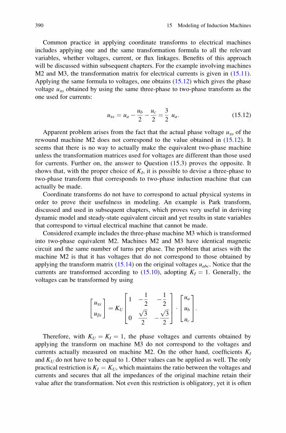
Common practice in applying coordinate transforms to electrical machines
includes applying one and the same transformation formula to all the relevant
variables, whether voltages, current, or flux linkages. Benefits of this approach
will be discussed within subsequent chapters. For the example involving machines
M2 and M3, the transformation matrix for electrical currents is given in (15.11).
Applying the same formula to voltages, one obtains (15.12) which gives the phase
voltage uas obtained by using the same three-phase to two-phase transform as the
one used for currents:
uas ¼ ua � ub2� uc
2¼ 3
2ua: (15.12)
Apparent problem arises from the fact that the actual phase voltage uas of therewound machine M2 does not correspond to the value obtained in (15.12). It
seems that there is no way to actually make the equivalent two-phase machine
unless the transformation matrices used for voltages are different than those used
for currents. Further on, the answer to Question (15.3) proves the opposite. It
shows that, with the proper choice of KI, it is possible to devise a three-phase to
two-phase transform that corresponds to two-phase induction machine that can
actually be made.
Coordinate transforms do not have to correspond to actual physical systems in
order to prove their usefulness in modeling. An example is Park transform,
discussed and used in subsequent chapters, which proves very useful in deriving
dynamic model and steady-state equivalent circuit and yet results in state variables
that correspond to virtual electrical machine that cannot be made.
Considered example includes the three-phase machine M3 which is transformed
into two-phase equivalent M2. Machines M2 and M3 have identical magnetic
circuit and the same number of turns per phase. The problem that arises with the
machine M2 is that it has voltages that do not correspond to those obtained by
applying the transform matrix (15.14) on the original voltages uabc. Notice that thecurrents are transformed according to (15.10), adopting KI ¼ 1. Generally, the
voltages can be transformed by using
uas
ubs
" #¼ KU
1 � 1
2� 1
2
0
ffiffiffi3
p
2�
ffiffiffi3
p
2
2664
3775 �
ua
ub
uc
264
375:
Therefore, with KU ¼ KI ¼ 1, the phase voltages and currents obtained by
applying the transform on machine M3 do not correspond to the voltages and
currents actually measured on machine M2. On the other hand, coefficients KI
and KU do not have to be equal to 1. Other values can be applied as well. The only
practical restriction is KI ¼ KU, which maintains the ratio between the voltages and
currents and secures that all the impedances of the original machine retain their
value after the transformation. Not even this restriction is obligatory, yet it is often
390 15 Modeling of Induction Machines
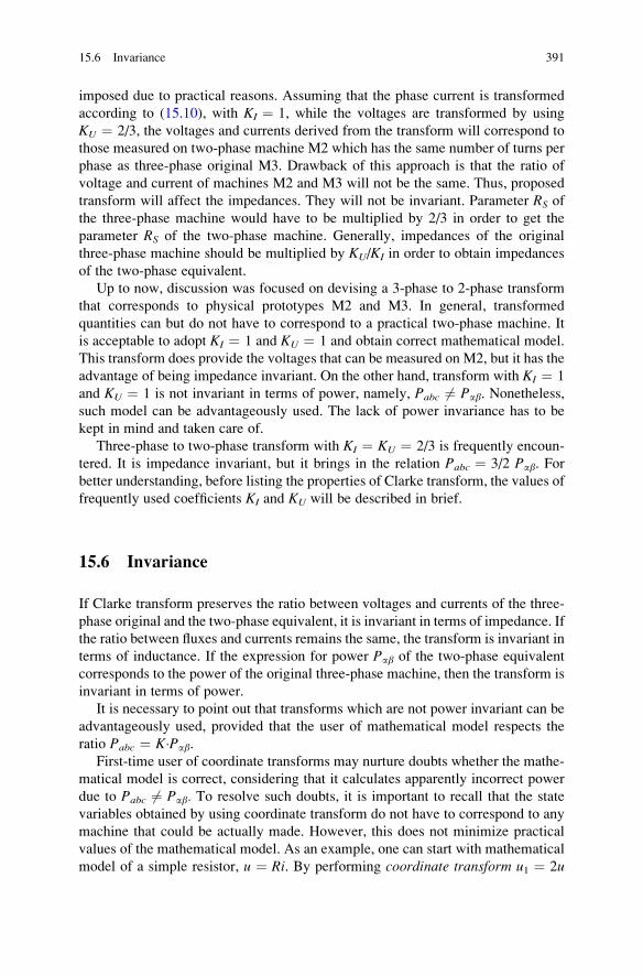
imposed due to practical reasons. Assuming that the phase current is transformed
according to (15.10), with KI ¼ 1, while the voltages are transformed by using
KU ¼ 2/3, the voltages and currents derived from the transform will correspond to
those measured on two-phase machine M2 which has the same number of turns per
phase as three-phase original M3. Drawback of this approach is that the ratio of
voltage and current of machines M2 and M3 will not be the same. Thus, proposed
transform will affect the impedances. They will not be invariant. Parameter RS of
the three-phase machine would have to be multiplied by 2/3 in order to get the
parameter RS of the two-phase machine. Generally, impedances of the original
three-phase machine should be multiplied by KU/KI in order to obtain impedances
of the two-phase equivalent.
Up to now, discussion was focused on devising a 3-phase to 2-phase transform
that corresponds to physical prototypes M2 and M3. In general, transformed
quantities can but do not have to correspond to a practical two-phase machine. It
is acceptable to adopt KI ¼ 1 and KU ¼ 1 and obtain correct mathematical model.
This transform does provide the voltages that can be measured on M2, but it has the
advantage of being impedance invariant. On the other hand, transform with KI ¼ 1
and KU ¼ 1 is not invariant in terms of power, namely, Pabc 6¼ Pab. Nonetheless,
such model can be advantageously used. The lack of power invariance has to be
kept in mind and taken care of.
Three-phase to two-phase transform with KI ¼ KU ¼ 2/3 is frequently encoun-
tered. It is impedance invariant, but it brings in the relation Pabc ¼ 3/2 Pab. For
better understanding, before listing the properties of Clarke transform, the values of
frequently used coefficients KI and KU will be described in brief.
15.6 Invariance
If Clarke transform preserves the ratio between voltages and currents of the three-
phase original and the two-phase equivalent, it is invariant in terms of impedance. If
the ratio between fluxes and currents remains the same, the transform is invariant in
terms of inductance. If the expression for power Pab of the two-phase equivalent
corresponds to the power of the original three-phase machine, then the transform is
invariant in terms of power.
It is necessary to point out that transforms which are not power invariant can be
advantageously used, provided that the user of mathematical model respects the
ratio Pabc ¼ K�Pab.
First-time user of coordinate transforms may nurture doubts whether the mathe-
matical model is correct, considering that it calculates apparently incorrect power
due to Pabc 6¼ Pab. To resolve such doubts, it is important to recall that the state
variables obtained by using coordinate transform do not have to correspond to any
machine that could be actually made. However, this does not minimize practical
values of the mathematical model. As an example, one can start with mathematical
model of a simple resistor, u ¼ Ri. By performing coordinate transform u1 ¼ 2u
15.6 Invariance 391
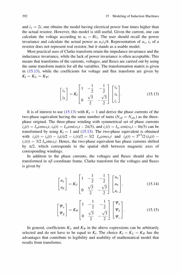
and i1 ¼ 2i, one obtains the model having electrical power four times higher than
the actual resistor. However, this model is still useful. Given the current, one can
calculate the voltage according to u1 ¼ Ri1. The user should recall the power
invariance and calculate the actual power as u1i1/4. Representation of u1, i1 of a
resistor does not represent real resistor, but it stands as a usable model.
Most practical uses of Clarke transform retain the impedance invariance and the
inductance invariance, while the lack of power invariance is often acceptable. This
means that transforms of the currents, voltages, and fluxes are carried out by using
the same transform matrix for all the variables. The transformation matrix is given
in (15.13), while the coefficients for voltage and flux transform are given by
KI ¼ KU ¼ KC:
ia
ib
" #¼ KI
1 � 1
2� 1
2
0
ffiffiffi3
p
2�
ffiffiffi3
p
2
2664
3775
ia
ib
ic
264
375: (15.13)
It is of interest to use (15.13) with KI ¼ 1 and derive the phase currents of the
two-phase equivalent having the same number of turns (Nab ¼ Nabc) as the three-
phase original. The three-phase winding with symmetrical set of phase currents
ia(t) ¼ Imcosoet, ib(t) ¼ Imcos(oet – 2p/3), and ic(t) ¼ Im cos(oet – 4p/3) can be
transformed by using KI ¼ 1 and (15.13). The two-phase equivalent is obtained
with ia(t) ¼ ia(t) � ib(t)/2 � ic(t)/2 ¼ 3/2 Imcosoet and ib(t) ¼ 30.5/2�(ib(t) �ic(t)) ¼ 3/2 Imsinoet. Hence, the two-phase equivalent has phase currents shifted
by p/2, which corresponds to the spatial shift between magnetic axes of
corresponding windings.
In addition to the phase currents, the voltages and fluxes should also be
transformed in ab coordinate frame. Clarke transform for the voltages and fluxes
is given by
ua
ub
" #¼ KU
1 � 1
2� 1
2
0
ffiffiffi3
p
2�
ffiffiffi3
p
2
2664
3775
ua
ub
uc
264
375; (15.14)
Ca
Cb
" #¼ KC
1 � 1
2� 1
2
0
ffiffiffi3
p
2�
ffiffiffi3
p
2
2664
3775
Ca
Cb
Cc
264
375: (15.15)
In general, coefficients KU and KC in the above expressions can be arbitrarily
selected and do not have to be equal to KI. The choice KI ¼ KU ¼ KC has the
advantages that contribute to legibility and usability of mathematical model that
results from transforms.
392 15 Modeling of Induction Machines
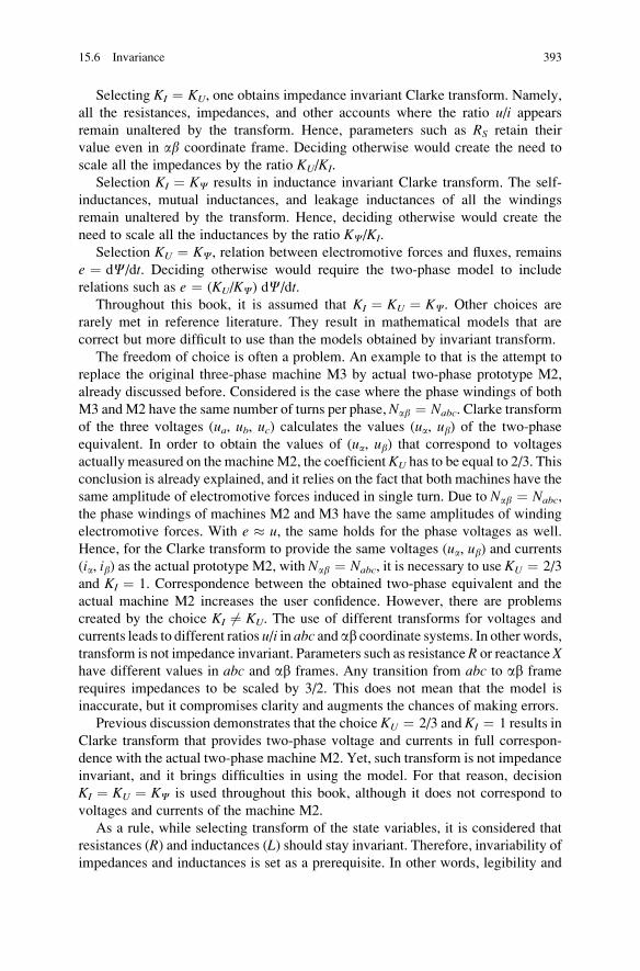
Selecting KI ¼ KU, one obtains impedance invariant Clarke transform. Namely,
all the resistances, impedances, and other accounts where the ratio u/i appearsremain unaltered by the transform. Hence, parameters such as RS retain their
value even in ab coordinate frame. Deciding otherwise would create the need to
scale all the impedances by the ratio KU/KI.
Selection KI ¼ KC results in inductance invariant Clarke transform. The self-
inductances, mutual inductances, and leakage inductances of all the windings
remain unaltered by the transform. Hence, deciding otherwise would create the
need to scale all the inductances by the ratio KC/KI.
Selection KU ¼ KC, relation between electromotive forces and fluxes, remains
e ¼ dC/dt. Deciding otherwise would require the two-phase model to include
relations such as e ¼ (KU/KC) dC/dt.Throughout this book, it is assumed that KI ¼ KU ¼ KC. Other choices are
rarely met in reference literature. They result in mathematical models that are
correct but more difficult to use than the models obtained by invariant transform.
The freedom of choice is often a problem. An example to that is the attempt to
replace the original three-phase machine M3 by actual two-phase prototype M2,
already discussed before. Considered is the case where the phase windings of both
M3 andM2 have the same number of turns per phase, Nab ¼ Nabc. Clarke transform
of the three voltages (ua, ub, uc) calculates the values (ua, ub) of the two-phase
equivalent. In order to obtain the values of (ua, ub) that correspond to voltages
actually measured on the machineM2, the coefficient KU has to be equal to 2/3. This
conclusion is already explained, and it relies on the fact that both machines have the
same amplitude of electromotive forces induced in single turn. Due to Nab ¼ Nabc,
the phase windings of machines M2 and M3 have the same amplitudes of winding
electromotive forces. With e � u, the same holds for the phase voltages as well.
Hence, for the Clarke transform to provide the same voltages (ua, ub) and currents
(ia, ib) as the actual prototype M2, with Nab ¼ Nabc, it is necessary to use KU ¼ 2/3
and KI ¼ 1. Correspondence between the obtained two-phase equivalent and the
actual machine M2 increases the user confidence. However, there are problems
created by the choice KI 6¼ KU. The use of different transforms for voltages and
currents leads to different ratios u/i in abc and ab coordinate systems. In other words,
transform is not impedance invariant. Parameters such as resistance R or reactance Xhave different values in abc and ab frames. Any transition from abc to ab frame
requires impedances to be scaled by 3/2. This does not mean that the model is
inaccurate, but it compromises clarity and augments the chances of making errors.
Previous discussion demonstrates that the choice KU ¼ 2/3 and KI ¼ 1 results in
Clarke transform that provides two-phase voltage and currents in full correspon-
dence with the actual two-phase machine M2. Yet, such transform is not impedance
invariant, and it brings difficulties in using the model. For that reason, decision
KI ¼ KU ¼ KC is used throughout this book, although it does not correspond to
voltages and currents of the machine M2.
As a rule, while selecting transform of the state variables, it is considered that
resistances (R) and inductances (L) should stay invariant. Therefore, invariability ofimpedances and inductances is set as a prerequisite. In other words, legibility and
15.6 Invariance 393
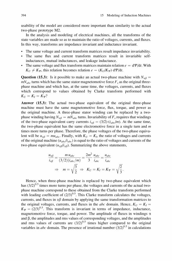
usability of the model are considered more important than similarity to the actual
two-phase prototype M2.
In the analysis and modeling of electrical machines, all the transforms of the
state variables are made so as to maintain the ratio of voltages, currents, and fluxes.
In this way, transforms are impedance invariant and inductance invariant.
• The same voltage and current transform matrices result impedance invariability.
• The same flux and current transform matrices result in invariable self-
inductances, mutual inductances, and leakage inductance.
• The same voltage and flux transform matrices maintain relation e ¼ dC/dt. With
KU 6¼ KC, this relation becomes relation e ¼ (KU/KC) dC/dt.
Question (15.3): Is it possible to make an actual two-phase machine with Nab ¼mNabc turns which has the same stator magnetomotive force Fs as the original three-
phase machine and which has, at the same time, the voltages, currents, and fluxes
which correspond to values obtained by Clarke transform performed with
KU ¼ KI ¼ KC?
Answer (15.3): The actual two-phase equivalent of the original three-phase
machine must have the same magnetomotive force, flux, torque, and power as
the original machine. A three-phase stator winding can be replaced by a two-
phase winding having Nab ¼ mNabc turns. Invariability of Fs requires that windings
of the two-phase equivalent carry currents iab ¼ (3/2)�(iabc/m). At the same time,
the two-phase equivalent has the same electromotive force in a single turn and mtimes more turns per phase. Therefore, the phase voltages of the two-phase equiva-
lent will be uab ¼ muabc. Finally, with KU ¼ KI, the ratio of voltages and currents
of the original machine (uabc/iabc) is equal to the ratio of voltages and currents of thetwo-phase equivalent (uab/iab). Summarizing the above statements,
uabiab
¼ muabc3=2ð Þ iabc=mð Þ ¼
2m2
3
uabciabc
¼ uabciabc
) m ¼ffiffiffiffi3
2
r) KU ¼ KI ¼ KC ¼
ffiffiffiffi2
3
r:
Hence, when three-phase machine is replaced by two-phase equivalent which
has (3/2)0.5 times more turns per phase, the voltages and currents of the actual two-
phase machine correspond to these obtained from the Clarke transform performed
with leading coefficient of (2/3)0.5. This Clarke transform calculates the voltages,
currents, and fluxes in ab domain by applying the same transformation matrices to
the original voltages, currents, and fluxes in the abc domain. Hence, KU ¼ KI ¼KC ¼ (2/3)0.5. This transform is invariant in terms of impedance, inductance,
magnetomotive force, torque, and power. The amplitude of fluxes in windings aand b, the amplitudes and rms values of corresponding voltages, and the amplitudes
and rms values of currents are (3/2)0.5 times higher compared to the original
variables in abc domain. The presence of irrational number (3/2)0.5 in calculations
394 15 Modeling of Induction Machines
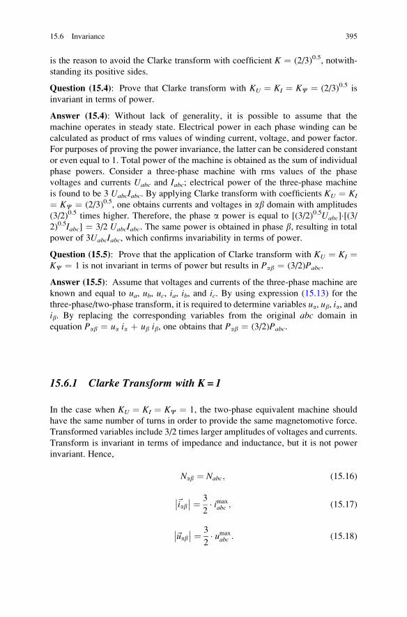
is the reason to avoid the Clarke transform with coefficient K ¼ (2/3)0.5, notwith-
standing its positive sides.
Question (15.4): Prove that Clarke transform with KU ¼ KI ¼ KC ¼ (2/3)0.5 is
invariant in terms of power.
Answer (15.4): Without lack of generality, it is possible to assume that the
machine operates in steady state. Electrical power in each phase winding can be
calculated as product of rms values of winding current, voltage, and power factor.
For purposes of proving the power invariance, the latter can be considered constant
or even equal to 1. Total power of the machine is obtained as the sum of individual
phase powers. Consider a three-phase machine with rms values of the phase
voltages and currents Uabc and Iabc; electrical power of the three-phase machine
is found to be 3 UabcIabc. By applying Clarke transform with coefficients KU ¼ KI
¼ KC ¼ (2/3)0.5, one obtains currents and voltages in ab domain with amplitudes
(3/2)0.5 times higher. Therefore, the phase a power is equal to [(3/2)0.5Uabc]�[(3/2)0.5Iabc] ¼ 3/2 UabcIabc. The same power is obtained in phase b, resulting in total
power of 3UabcIabc, which confirms invariability in terms of power.
Question (15.5): Prove that the application of Clarke transform with KU ¼ KI ¼KC ¼ 1 is not invariant in terms of power but results in Pab ¼ (3/2)Pabc.
Answer (15.5): Assume that voltages and currents of the three-phase machine are
known and equal to ua, ub, uc, ia, ib, and ic. By using expression (15.13) for the
three-phase/two-phase transform, it is required to determine variables ua, ub, ia, andib. By replacing the corresponding variables from the original abc domain in
equation Pab ¼ ua ia þ ub ib, one obtains that Pab ¼ (3/2)Pabc.
15.6.1 Clarke Transform with K= 1
In the case when KU ¼ KI ¼ KC ¼ 1, the two-phase equivalent machine should
have the same number of turns in order to provide the same magnetomotive force.
Transformed variables include 3/2 times larger amplitudes of voltages and currents.
Transform is invariant in terms of impedance and inductance, but it is not power
invariant. Hence,
Nab ¼ Nabc; (15.16)
~iab�� �� ¼ 3
2� imax
abc ; (15.17)
~uab�� �� ¼ 3
2� umax
abc : (15.18)
15.6 Invariance 395
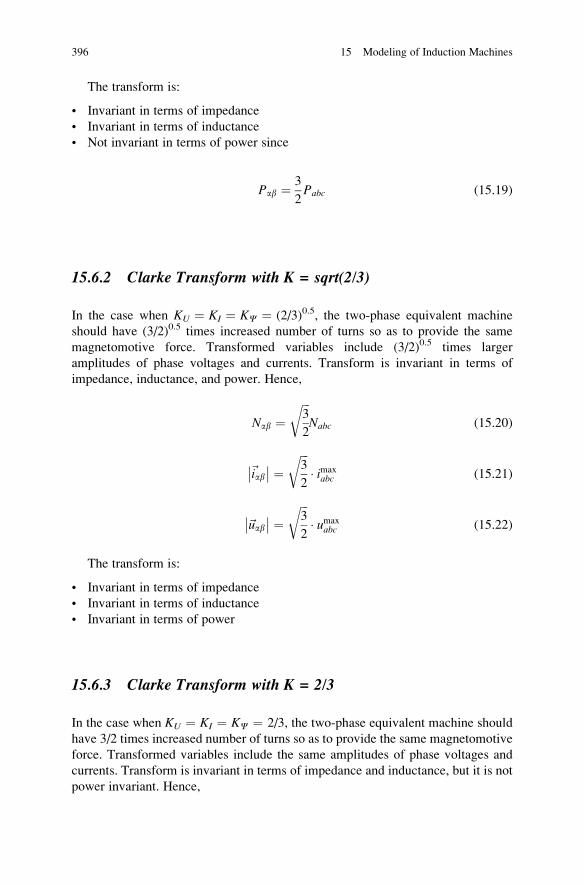
The transform is:
• Invariant in terms of impedance
• Invariant in terms of inductance
• Not invariant in terms of power since
Pab ¼ 3
2Pabc (15.19)
15.6.2 Clarke Transform with K = sqrt(2/3)
In the case when KU ¼ KI ¼ KC ¼ (2/3)0.5, the two-phase equivalent machine
should have (3/2)0.5 times increased number of turns so as to provide the same
magnetomotive force. Transformed variables include (3/2)0.5 times larger
amplitudes of phase voltages and currents. Transform is invariant in terms of
impedance, inductance, and power. Hence,
Nab ¼ffiffiffi3
2
rNabc (15.20)
~iab�� �� ¼
ffiffiffi3
2
r� imax
abc (15.21)
~uab�� �� ¼
ffiffiffi3
2
r� umax
abc (15.22)
The transform is:
• Invariant in terms of impedance
• Invariant in terms of inductance
• Invariant in terms of power
15.6.3 Clarke Transform with K = 2/3
In the case when KU ¼ KI ¼ KC ¼ 2/3, the two-phase equivalent machine should
have 3/2 times increased number of turns so as to provide the same magnetomotive
force. Transformed variables include the same amplitudes of phase voltages and
currents. Transform is invariant in terms of impedance and inductance, but it is not
power invariant. Hence,
396 15 Modeling of Induction Machines
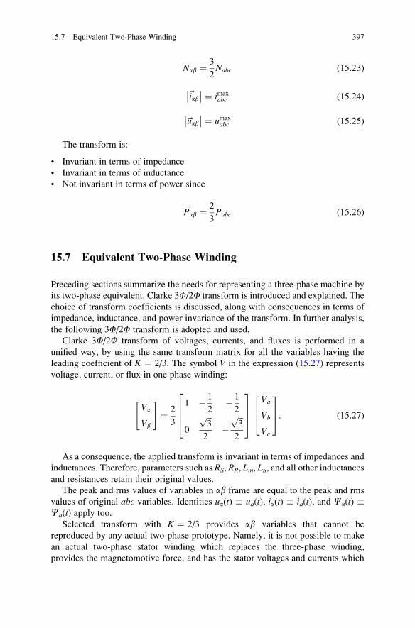
Nab ¼ 3
2Nabc (15.23)
~iab�� �� ¼ imax
abc (15.24)
~uab�� �� ¼ umax
abc (15.25)
The transform is:
• Invariant in terms of impedance
• Invariant in terms of inductance
• Not invariant in terms of power since
Pab ¼ 2
3Pabc (15.26)
15.7 Equivalent Two-Phase Winding
Preceding sections summarize the needs for representing a three-phase machine by
its two-phase equivalent. Clarke 3F/2F transform is introduced and explained. The
choice of transform coefficients is discussed, along with consequences in terms of
impedance, inductance, and power invariance of the transform. In further analysis,
the following 3F/2F transform is adopted and used.
Clarke 3F/2F transform of voltages, currents, and fluxes is performed in a
unified way, by using the same transform matrix for all the variables having the
leading coefficient of K ¼ 2/3. The symbol V in the expression (15.27) represents
voltage, current, or flux in one phase winding:
Va
Vb
" #¼ 2
3
1 � 1
2� 1
2
0
ffiffiffi3
p
2�
ffiffiffi3
p
2
2664
3775
Va
Vb
Vc
264
375: (15.27)
As a consequence, the applied transform is invariant in terms of impedances and
inductances. Therefore, parameters such as RS, RR, Lm, LS, and all other inductancesand resistances retain their original values.
The peak and rms values of variables in ab frame are equal to the peak and rms
values of original abc variables. Identities ua(t) � ua(t), ia(t) � ia(t), and Ca(t) �Ca(t) apply too.
Selected transform with K ¼ 2/3 provides ab variables that cannot be
reproduced by any actual two-phase prototype. Namely, it is not possible to make
an actual two-phase stator winding which replaces the three-phase winding,
provides the magnetomotive force, and has the stator voltages and currents which
15.7 Equivalent Two-Phase Winding 397
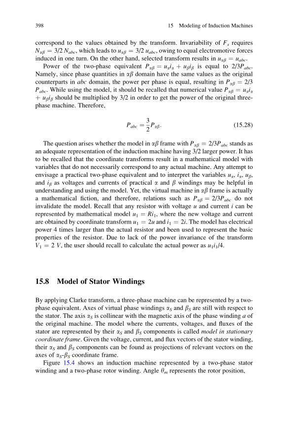
correspond to the values obtained by the transform. Invariability of Fs requires
Nab ¼ 3/2 Nabc, which leads to uab ¼ 3/2 uabc, owing to equal electromotive forces
induced in one turn. On the other hand, selected transform results in uab ¼ uabc.Power of the two-phase equivalent Pab ¼ uaia þ ubib is equal to 2/3Pabc.
Namely, since phase quantities in ab domain have the same values as the original
counterparts in abc domain, the power per phase is equal, resulting in Pab ¼ 2/3
Pabc. While using the model, it should be recalled that numerical value Pab ¼ uaiaþ ubib should be multiplied by 3/2 in order to get the power of the original three-
phase machine. Therefore,
Pabc ¼ 3
2Pab: (15.28)
The question arises whether the model in ab frame with Pab ¼ 2/3Pabc stands as
an adequate representation of the induction machine having 3/2 larger power. It has
to be recalled that the coordinate transforms result in a mathematical model with
variables that do not necessarily correspond to any actual machine. Any attempt to
envisage a practical two-phase equivalent and to interpret the variables ua, ia, ub,and ib as voltages and currents of practical a and b windings may be helpful in
understanding and using the model. Yet, the virtual machine in ab frame is actually
a mathematical fiction, and therefore, relations such as Pab ¼ 2/3Pabc do not
invalidate the model. Recall that any resistor with voltage u and current i can be
represented by mathematical model u1 ¼ Ri1, where the new voltage and current
are obtained by coordinate transform u1 ¼ 2u and i1 ¼ 2i. The model has electrical
power 4 times larger than the actual resistor and been used to represent the basic
properties of the resistor. Due to lack of the power invariance of the transform
V1 ¼ 2 V, the user should recall to calculate the actual power as u1i1/4.
15.8 Model of Stator Windings
By applying Clarke transform, a three-phase machine can be represented by a two-
phase equivalent. Axes of virtual phase windings aS and bS are still with respect to
the stator. The axis aS is collinear with the magnetic axis of the phase winding a of
the original machine. The model where the currents, voltages, and fluxes of the
stator are represented by their aS and bS components is called model in stationarycoordinate frame. Given the voltage, current, and flux vectors of the stator winding,their aS and bS components can be found as projections of relevant vectors on the
axes of aS-bS coordinate frame.
Figure 15.4 shows an induction machine represented by a two-phase stator
winding and a two-phase rotor winding. Angle ym represents the rotor position,
398 15 Modeling of Induction Machines
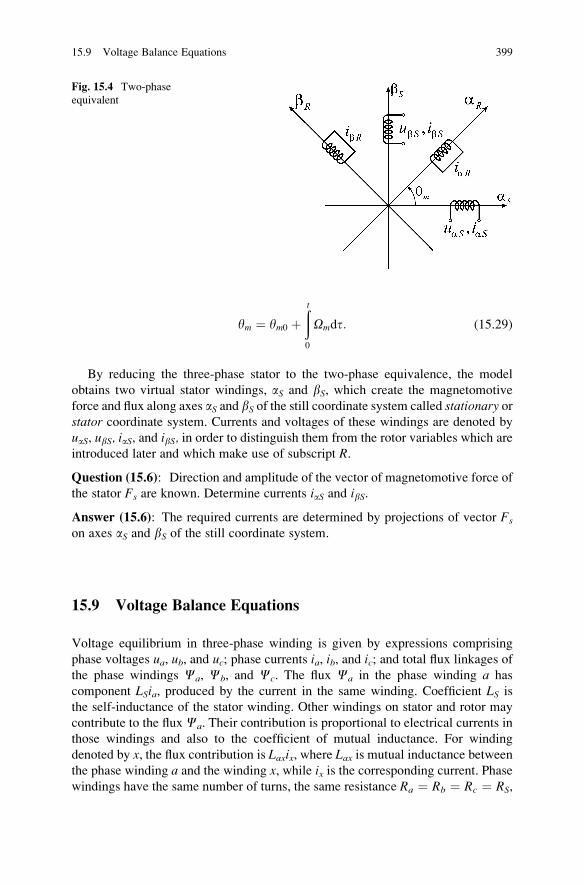
ym ¼ ym0 þðt
0
Omdt: (15.29)
By reducing the three-phase stator to the two-phase equivalence, the model
obtains two virtual stator windings, aS and bS, which create the magnetomotive
force and flux along axes aS and bS of the still coordinate system called stationary orstator coordinate system. Currents and voltages of these windings are denoted by
uaS, ubS, iaS, and ibS, in order to distinguish them from the rotor variables which are
introduced later and which make use of subscript R.
Question (15.6): Direction and amplitude of the vector of magnetomotive force of
the stator Fs are known. Determine currents iaS and ibS.
Answer (15.6): The required currents are determined by projections of vector Fs
on axes aS and bS of the still coordinate system.
15.9 Voltage Balance Equations
Voltage equilibrium in three-phase winding is given by expressions comprising
phase voltages ua, ub, and uc; phase currents ia, ib, and ic; and total flux linkages of
the phase windings Ca, Cb, and Cc. The flux Ca in the phase winding a has
component LSia, produced by the current in the same winding. Coefficient LS is
the self-inductance of the stator winding. Other windings on stator and rotor may
contribute to the fluxCa. Their contribution is proportional to electrical currents in
those windings and also to the coefficient of mutual inductance. For winding
denoted by x, the flux contribution is Laxix, where Lax is mutual inductance between
the phase winding a and the winding x, while ix is the corresponding current. Phasewindings have the same number of turns, the same resistance Ra ¼ Rb ¼ Rc ¼ RS,
Fig. 15.4 Two-phase
equivalent
15.9 Voltage Balance Equations 399
and the same coefficients of self-inductance La ¼ Lb ¼ Lc ¼ LS. For any windings,the voltage, current, and flux are tied by relation u ¼ Ri þ dC/dt. Therefore,
ua ¼ RSia þ dCa=dt;
ub ¼ RSib þ dCb=dt; )uc ¼ RSic þ dCc=dt:
uaubuc
24
35 ¼
RS 0 0
0 RS 0
0 0 RS
24
35 ia
icic
24
35þ d
dt
Ca
Cb
Cc
24
35: (15.30)
By applying Clarke transform which uses the same transformation matrix for the
voltages, currents, and fluxes, the voltage balance equations can be transferred to
aS–bS coordinate frame and expressed in terms of aS and bS projections of the
voltage, current, and flux vectors. Quantities CaS and CbS are projections of
the stator flux vector on axes aS and bS. They can be calculated by applying the
three-phase/two-phase transform to the total fluxes of the phase windings Ca, Cb,
andCc. Moreover, the transformation matrix can be applied to the whole right side
of (15.30), obtaining in this way:
uaS ¼ RSiaS þ dCaS=dt;
ubS ¼ RSibS þ dCbS=dt: (15.31)
The above equation represents the voltage equilibrium in the two-phase equiva-
lent of the stator winding. In addition to modeling the stator, it is required to model
the short-circuited rotor cage. Voltage equilibrium equations in the rotor circuit will
complete the model of the electrical subsystem of the induction machine.
15.10 Modeling Rotor Cage
The rotor cage contains a relatively large number of conductors which are short
circuited by the front and rear rings. An example of the rotor cage separated from the
rotor magnetic circuit is shown in Fig. 15.5a. For rotor cage with NR ¼ 28
conductors, it is possible to identify 14 short-circuited turns, each created by one
pair of diametrically positioned conductors. Therefore, it is possible tomake amodel
of the rotor comprising 14 short-circuited turns with mutual magnetic coupling, also
coupled with aS and bS stator windings, as shown in Fig. 15.5b. However, such
model would be of little practical value. Its inductance matrix will have dimensions
16 � 16. Therefore, another approach is needed to model the rotor cage.
As the first step, it is of interest to observe the part (c) in Fig. 15.5 and assume
that the rotor flux pulsates along the vertical axis. At this point, it is of interest to
400 15 Modeling of Induction Machines
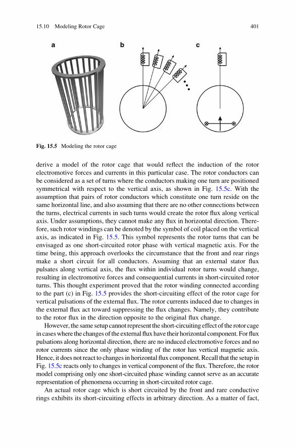
derive a model of the rotor cage that would reflect the induction of the rotor
electromotive forces and currents in this particular case. The rotor conductors can
be considered as a set of turns where the conductors making one turn are positioned
symmetrical with respect to the vertical axis, as shown in Fig. 15.5c. With the
assumption that pairs of rotor conductors which constitute one turn reside on the
same horizontal line, and also assuming that there are no other connections between
the turns, electrical currents in such turns would create the rotor flux along vertical
axis. Under assumptions, they cannot make any flux in horizontal direction. There-
fore, such rotor windings can be denoted by the symbol of coil placed on the vertical
axis, as indicated in Fig. 15.5. This symbol represents the rotor turns that can be
envisaged as one short-circuited rotor phase with vertical magnetic axis. For the
time being, this approach overlooks the circumstance that the front and rear rings
make a short circuit for all conductors. Assuming that an external stator flux
pulsates along vertical axis, the flux within individual rotor turns would change,
resulting in electromotive forces and consequential currents in short-circuited rotor
turns. This thought experiment proved that the rotor winding connected according
to the part (c) in Fig. 15.5 provides the short-circuiting effect of the rotor cage for
vertical pulsations of the external flux. The rotor currents induced due to changes in
the external flux act toward suppressing the flux changes. Namely, they contribute
to the rotor flux in the direction opposite to the original flux change.
However, the same setup cannot represent the short-circuiting effect of the rotor cage
in caseswhere the changes of the external fluxhave their horizontal component. For flux
pulsations along horizontal direction, there are no induced electromotive forces and no
rotor currents since the only phase winding of the rotor has vertical magnetic axis.
Hence, it does not react to changes in horizontal flux component. Recall that the setup in
Fig. 15.5c reacts only to changes in vertical component of the flux. Therefore, the rotor
model comprising only one short-circuited phase winding cannot serve as an accurate
representation of phenomena occurring in short-circuited rotor cage.
An actual rotor cage which is short circuited by the front and rare conductive
rings exhibits its short-circuiting effects in arbitrary direction. As a matter of fact,
Fig. 15.5 Modeling the rotor cage
15.10 Modeling Rotor Cage 401
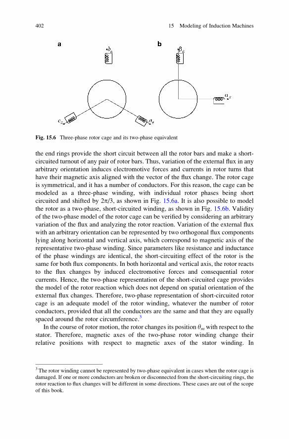
the end rings provide the short circuit between all the rotor bars and make a short-
circuited turnout of any pair of rotor bars. Thus, variation of the external flux in any
arbitrary orientation induces electromotive forces and currents in rotor turns that
have their magnetic axis aligned with the vector of the flux change. The rotor cage
is symmetrical, and it has a number of conductors. For this reason, the cage can be
modeled as a three-phase winding, with individual rotor phases being short
circuited and shifted by 2p/3, as shown in Fig. 15.6a. It is also possible to model
the rotor as a two-phase, short-circuited winding, as shown in Fig. 15.6b. Validity
of the two-phase model of the rotor cage can be verified by considering an arbitrary
variation of the flux and analyzing the rotor reaction. Variation of the external flux
with an arbitrary orientation can be represented by two orthogonal flux components
lying along horizontal and vertical axis, which correspond to magnetic axis of the
representative two-phase winding. Since parameters like resistance and inductance
of the phase windings are identical, the short-circuiting effect of the rotor is the
same for both flux components. In both horizontal and vertical axis, the rotor reacts
to the flux changes by induced electromotive forces and consequential rotor
currents. Hence, the two-phase representation of the short-circuited cage provides
the model of the rotor reaction which does not depend on spatial orientation of the
external flux changes. Therefore, two-phase representation of short-circuited rotor
cage is an adequate model of the rotor winding, whatever the number of rotor
conductors, provided that all the conductors are the same and that they are equally
spaced around the rotor circumference.3
In the course of rotor motion, the rotor changes its position ymwith respect to the
stator. Therefore, magnetic axes of the two-phase rotor winding change their
relative positions with respect to magnetic axes of the stator winding. In
Fig. 15.6 Three-phase rotor cage and its two-phase equivalent
3 The rotor winding cannot be represented by two-phase equivalent in cases when the rotor cage is
damaged. If one or more conductors are broken or disconnected from the short-circuiting rings, the
rotor reaction to flux changes will be different in some directions. These cases are out of the scope
of this book.
402 15 Modeling of Induction Machines
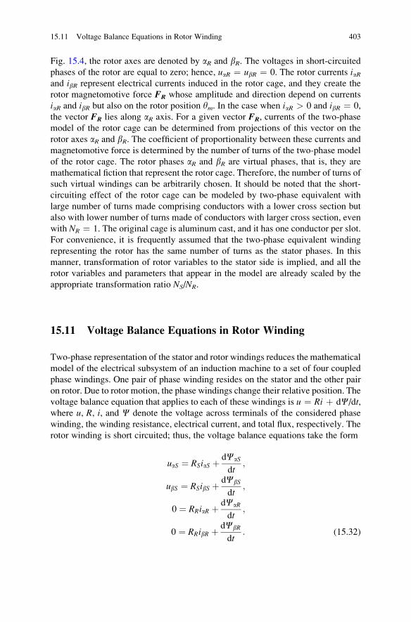
Fig. 15.4, the rotor axes are denoted by aR and bR. The voltages in short-circuited
phases of the rotor are equal to zero; hence, uaR ¼ ubR ¼ 0. The rotor currents iaRand ibR represent electrical currents induced in the rotor cage, and they create the
rotor magnetomotive force FR whose amplitude and direction depend on currents
iaR and ibR but also on the rotor position ym. In the case when iaR > 0 and ibR ¼ 0,
the vector FR lies along aR axis. For a given vector FR, currents of the two-phase
model of the rotor cage can be determined from projections of this vector on the
rotor axes aR and bR. The coefficient of proportionality between these currents and
magnetomotive force is determined by the number of turns of the two-phase model
of the rotor cage. The rotor phases aR and bR are virtual phases, that is, they are
mathematical fiction that represent the rotor cage. Therefore, the number of turns of
such virtual windings can be arbitrarily chosen. It should be noted that the short-
circuiting effect of the rotor cage can be modeled by two-phase equivalent with
large number of turns made comprising conductors with a lower cross section but
also with lower number of turns made of conductors with larger cross section, even
with NR ¼ 1. The original cage is aluminum cast, and it has one conductor per slot.
For convenience, it is frequently assumed that the two-phase equivalent winding
representing the rotor has the same number of turns as the stator phases. In this
manner, transformation of rotor variables to the stator side is implied, and all the
rotor variables and parameters that appear in the model are already scaled by the
appropriate transformation ratio NS/NR.
15.11 Voltage Balance Equations in Rotor Winding
Two-phase representation of the stator and rotor windings reduces the mathematical
model of the electrical subsystem of an induction machine to a set of four coupled
phase windings. One pair of phase winding resides on the stator and the other pair
on rotor. Due to rotor motion, the phase windings change their relative position. The
voltage balance equation that applies to each of these windings is u ¼ Ri þ dC/dt,where u, R, i, and C denote the voltage across terminals of the considered phase
winding, the winding resistance, electrical current, and total flux, respectively. The
rotor winding is short circuited; thus, the voltage balance equations take the form
uaS ¼ RSiaS þ dCaS
dt;
ubS ¼ RSibS þ dCbS
dt;
0 ¼ RRiaR þ dCaR
dt;
0 ¼ RRibR þ dCbR
dt: (15.32)
15.11 Voltage Balance Equations in Rotor Winding 403
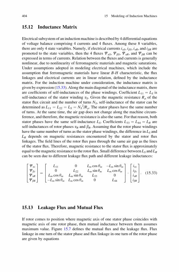
15.12 Inductance Matrix
Electrical subsystem of an inductionmachine is described by 4 differential equations
of voltage balance comprising 4 currents and 4 fluxes. Among these 8 variables,
there are only 4 state variables. Namely, if electrical currents iaS, ibS, iaR, and ibR arepromoted to the state variables, then the 4 fluxes CaS, CbS, CaR, and CbR can be
expressed in terms of currents. Relation between the fluxes and currents is generally
nonlinear, due to nonlinearity of ferromagnetic materials and magnetic saturations.
Under assumptions adopted in modeling electrical machines, which include the
assumption that ferromagnetic materials have linear B-H characteristic, the flux
linkages and electrical currents are in linear relation, defined by the inductance
matrix. For the induction machine under consideration, the inductance matrix is
given by expression (15.33). Along themain diagonal of the inductancematrix, there
are coefficients of self-inductances of the phase windings. Coefficient L11 ¼ LS isself-inductance of the stator winding aS. Given the magnetic resistance Rm of the
stator flux circuit and the number of turns NS, self-inductance of the stator can be
determined as L11 ¼ L22 ¼ LS ¼ NS2/Rm. The stator phases have the same number
of turns. At the same time, the air gap does not change along the machine circum-
ference, and therefore, the magnetic resistance is also the same. For that reason, both
stator phases have the same self-inductance LS. Coefficients L33 ¼ L44 ¼ LR are
self-inductances of rotor phases aR and bR. Assuming that the rotor phase windings
have the same number of turns as the stator phase windings, the difference in LS andLR depends on magnetic resistances encountered by the stator and rotor flux
linkages. The field lines of the rotor flux pass through the same air gap as the lines
of the stator flux. Therefore, magnetic resistance to the stator flux is approximately
equal to the magnetic resistance to the rotor flux. Small difference between LS and LRcan be seen due to different leakage flux path and different leakage inductances:
Cas
Cbs
CaR
CbR
2664
3775 ¼
L11 0 Lm cos ym �Lm sin ym0 L22 Lm sin ym Lm cos ym
Lm cos ym Lm sin ym L33 0
�Lm sin ym Lm cos ym 0 L44
2664
3775 �
iasibsiaRibR
2664
3775: (15.33)
15.13 Leakage Flux and Mutual Flux
If rotor comes to position where magnetic axis of one stator phase coincides with
magnetic axis of one rotor phase, then mutual inductance between them assumes
maximum value. Figure 15.7 defines the mutual flux and the leakage flux. Flux
linkage in one turn of the stator phase and flux linkage in one turn of the rotor phase
are given by equations
404 15 Modeling of Induction Machines
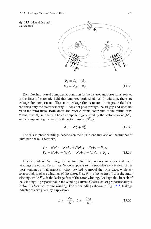
FS ¼ FgS þ Fm;
FR ¼ FgR þ Fm: (15.34)
Each flux has mutual component, common for both stator and rotor turns, related
to the lines of magnetic field that embrace both windings. In addition, there are
leakage flux components. The stator leakage flux is related to magnetic field that
encircles only the stator winding. It does not pass through the air gap and does not
reach the rotor turns. Both stator and rotor currents contribute to the mutual flux.
Mutual flux Fm in one turn has a component generated by the stator current (FSm)
and a component generated by the rotor current (FRm),
Fm ¼ FSm þ FR
m: (15.35)
The flux in phase windings depends on the flux in one turn and on the number of
turns per phase. Therefore,
CS ¼ NSFS ¼ NSFm þ NSFgS ¼ NSFm þCgS;
CR ¼ NRFR ¼ NRFm þ NRFgR ¼ NRFm þCgR: (15.36)
In cases where NS ¼ NR, the mutual flux components in stator and rotor
windings are equal. Recall that NR corresponds to the two-phase equivalent of the
rotor winding, a mathematical fiction devised to model the rotor cage, while NS
corresponds to phase windings of the stator. FluxCgS is the leakage flux of the statorwinding, whileCgR is the leakage flux of the rotor winding. Leakage flux in each of
the windings is proportional to the winding current. Coefficient of proportionality is
leakage inductance of the winding. For the windings shown in Fig. 15.7, leakage
inductances are given by expression
LgS ¼ CgS
iS; LgR ¼ CgR
iR: (15.37)
Fig. 15.7 Mutual flux and
leakage flux
15.13 Leakage Flux and Mutual Flux 405
Mutual inductance of stator and rotor windings in aligned position equals
Lm ¼ LSR ¼ NSFRm
iR¼ LRS ¼ NRFS
m
iS: (15.38)
Self-inductance of phase winding can be determined as the quotient of the
winding flux and the winding current, wherein the flux is caused only by the current
of the winding and does not get affected by other windings currents. This flux is
mutual in one part, while the remaining part is leakage flux. Self-inductances of the
stator and rotor are
LS ¼ NSFSm þ NSFgS
iS¼ NSFS
m þCgS
iS¼ NS
NRLRS þ LgS ¼ NS
NRLm þ LgS;
LR ¼ NRFRm þ NRFgR
iR¼ NRFR
m þCgR
iR¼ NR
NSLSR þ LgR ¼ NR
NSLm þ LgR: (15.39)
Therefore, leakage inductances make one part of self-inductances of phase
windings. Leakage inductance is higher in the case when magnetic coupling of
the two windings is weaker. In the case when the number of turns of the stator and
rotor is equal, as well as in the case when the rotor quantities are transformed to thestator side, the preceding equation takes the form
LS ¼ Lm þ LgS;
LR ¼ Lm þ LgR: (15.40)
15.14 Magnetic Coupling
Leakage flux of the stator and leakage flux of the rotor exist in different magnetic
circuits, and they may have different magnetic resistances. For that reason, even the
leakage inductances can be different.
Gross part of the stator flux encircles both stator and rotor windings, but there are
also some lines of magnetic field that encircle only the stator conductors. They do
not cross the air gap and thus do not encircle the rotor conductors. These field lines
belong to the leakage flux of the stator. Leakage flux of the stator is a smaller part of
the stator flux FS ¼ (LSiS)/NS. Leakage flux of the rotor is defined in similar.
Different shapes of the stator and rotor slots as well as differences in the shape
and cross section of conductors may result in different magnetic resistances on the
path of the stator and rotor leakage fluxes.
406 15 Modeling of Induction Machines
Magnetic resistance encountered on the path of the mutual flux is one and the
same for both stator and rotor phase windings. In both cases, mutual flux passes
through the air gap, where the gross part of the magnetic resistance is encountered.
Besides, mutual flux encircles both stator and rotor windings, passing through teeth,
yoke, and other parts of stator and rotor magnetic circuits. On the other hand,
magnetic resistance encountered along the path of leakage flux component is likely
to be different on stator and rotor. Namely, the leakage flux path includes the width
of the slots, and these are likely to be different. In general, a narrower slot opening
results in a smaller magnetic resistance for the leakage flux and a larger leakage
inductance, while a wide slot opening leads to a small leakage inductance.
In electrical machines, the power of electromechanical conversion and the
electromagnetic torque depend on the magnetic coupling between the stator and
rotor windings. Better coupling leads to more torque and power, hence the intention
to keep the leakage as low as possible. Ideally, the coefficient of magnetic coupling
of the stator and rotor k ¼ Lm/(LSLR)0,5 should reach unity. The leakage flux is
proportional to difference 1 � k, and in this case, it reaches zero as well as the
leakage inductance coefficients LgS and LgR. Practical machines cannot be designed
to achieve the coupling coefficient of 1. Such a coupling would require the
conductors of the two windings to be next to each other, so as to prevent any
leakage flux, and this is not feasible due to practical reasons. The stator and rotor
have to be separated by air gap for mechanical and electrical reasons. In machines
designed for operation with higher voltages, insulation of individual conductors and
windings has to sustain high-voltage stresses. For this reason, insulation layers are
thicker, as well as distances between individual conductors. With increased
distances between corresponding conductors, the space for the leakage flux is
enlarged as well as the leakage flux. Provisional values of the coupling coefficient
in low-voltage electrical machines (400 V, 50 Hz) are k ~ [0.9 .. 0.98]. In machines
designed to operate with high voltages, the values of the coupling coefficient could
be considerably lower, even k < 0.9.
15.15 Matrix L
Inductance matrix provides the link between the vector column with four total flux
linkages and the vector column with four electrical currents. On the main diagonal,
inductance matrix has the coefficients of self-inductances. Off the main diagonal, it
has the mutual inductances. The mutual inductances describing magnetic coupling
between stator and rotor phases are variable. They change in the course of motion.
Neglecting the differences in magnetic resistances for stator and rotor flux
linkages, the ratio LS/LR depends on the number of stator and rotor turns, L11 ¼ L22¼ LS ¼ NS
2/Rm, L33 ¼ L44 ¼ LR ¼ NR2/Rm. Self-inductances are strictly positive,
while mutual inductances may assume negative values as well as positive. Mutual
inductance Ljk determines the flux contribution brought into the phase winding k by
15.15 Matrix L 407
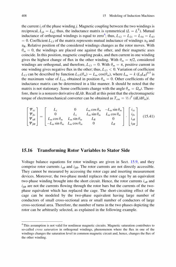
the current ij of the phase winding j. Magnetic coupling between the two windings is
reciprocal, Ljk ¼ Lkj; thus, the inductance matrix is symmetrical (L ¼ LT). Mutual
inductance of orthogonal windings is equal to zero4; thus, L12 ¼ L21 ¼ L34 ¼ L43¼ 0. Coefficient L13 of the matrix represents mutual inductance of windings aS andaR. Relative position of the considered windings changes as the rotor moves. With
ym ¼ 0, the windings are placed one against the other, and their magnetic axes
coincide. In this position, magnetic coupling peaks, and then current in one winding
gives the highest change of flux in the other winding. With ym ¼ p/2, consideredwindings are orthogonal, and therefore, L13 ¼ 0. With ym ¼ p, positive current inone winding gives negative flux in the other; thus, L13 < 0. Variation of coefficient
L13 can be described by function L13(ym) ¼ Lm cos(ym), where Lm ¼ k (LSLR)0.5 is
the maximum value of L13, obtained in position ym ¼ 0. Other coefficients of the
inductance matrix can be determined in a like manner. It should be noted that the
matrix is not stationary. Some coefficients change with the angle ym ¼ Omt. There-fore, there is a nonzero derivative dL/dt. Recall at this point that the electromagnetic
torque of electromechanical converter can be obtained as Tem ¼ ½ iT (dL/dym)i.
Cas
Cbs
CaR
CbR
2664
3775 ¼
Ls 0 Lm cos ym �Lm sin ym0 Ls Lm sin ym Lm cos ym
Lm cos ym Lm sin ym LR 0
�Lm sin ym Lm cos ym 0 LR
2664
3775 �
iasibsiaRibR
2664
3775 (15.41)
15.16 Transforming Rotor Variables to Stator Side
Voltage balance equations for rotor windings are given in Sect. 15.9, and they
comprise rotor currents iaR and ibR. The rotor currents are not directly accessible.
They cannot be measured by accessing the rotor cage and inserting measurement
devices. Moreover, the two-phase model replaces the rotor cage by an equivalent
two-phase winding brought into the short circuit. Hence, the rotor currents iaR and
ibR are not the currents flowing through the rotor bars but the currents of the two-
phase equivalent which has replaced the cage. The short-circuiting effect of the
cage can be modeled by the two-phase equivalent having large number of
conductors of small cross-sectional area or small number of conductors of large
cross-sectional area. Therefore, the number of turns in the two phases depicting the
rotor can be arbitrarily selected, as explained in the following example.
4 This assumption is not valid for nonlinear magnetic circuits. Magnetic saturation contributes to
so-called cross saturation in orthogonal windings, phenomenon where the flux in one of the
windings changes the saturation level in common magnetic circuit and, hence, changes the flux of
the other winding.
408 15 Modeling of Induction Machines
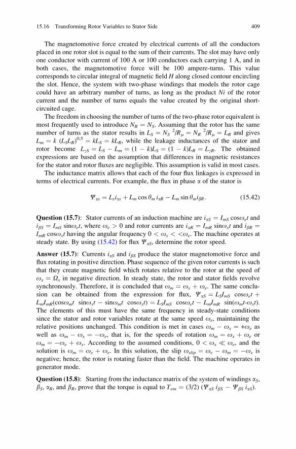
The magnetomotive force created by electrical currents of all the conductors
placed in one rotor slot is equal to the sum of their currents. The slot may have only
one conductor with current of 100 A or 100 conductors each carrying 1 A, and in
both cases, the magnetomotive force will be 100 ampere-turns. This value
corresponds to circular integral of magnetic field H along closed contour encircling
the slot. Hence, the system with two-phase windings that models the rotor cage
could have an arbitrary number of turns, as long as the product Ni of the rotor
current and the number of turns equals the value created by the original short-
circuited cage.
The freedom in choosing the number of turns of the two-phase rotor equivalent is
most frequently used to introduce NR ¼ NS. Assuming that the rotor has the same
number of turns as the stator results in LS ¼ NS2/Rm ¼ NR
2/Rm ¼ LR and gives
Lm ¼ k (LSLR)0,5 ¼ kLS ¼ kLR, while the leakage inductances of the stator and
rotor become LgS ¼ LS � Lm ¼ (1 � k)LS ¼ (1 � k)LR ¼ LgR. The obtained
expressions are based on the assumption that differences in magnetic resistances
for the stator and rotor fluxes are negligible. This assumption is valid in most cases.
The inductance matrix allows that each of the four flux linkages is expressed in
terms of electrical currents. For example, the flux in phase a of the stator is
Cas ¼ Lsias þ Lm cos ym iaR � Lm sin ymibR: (15.42)
Question (15.7): Stator currents of an induction machine are iaS ¼ ImS cosoet andibS ¼ ImS sinoet, where oe > 0 and rotor currents are iaR ¼ ImR sinoxt and ibR ¼ImR cosoxt having the angular frequency 0 < ox < <oe. The machine operates at
steady state. By using (15.42) for flux CaS, determine the rotor speed.
Answer (15.7): Currents iaS and ibS produce the stator magnetomotive force and
flux rotating in positive direction. Phase sequence of the given rotor currents is such
that they create magnetic field which rotates relative to the rotor at the speed of
ox ¼ Ox in negative direction. In steady state, the rotor and stator fields revolve
synchronously. Therefore, it is concluded that om ¼ ox þ oe. The same conclu-
sion can be obtained from the expression for flux, CaS ¼ LSImS cosoet þLmImR(cosomt sinoxt � sinomt cosoxt) ¼ LSImS cosoet � LmImR sin(omt-oxt).The elements of this must have the same frequency in steady-state conditions
since the stator and rotor variables rotate at the same speed oe, maintaining the
relative positions unchanged. This condition is met in cases om � ox ¼ +oe as
well as om � ox ¼ �oe, that is, for the speeds of rotation om ¼ ox þ oe or
om ¼ �oe þ ox. According to the assumed conditions, 0 < ox � oe, and the
solution is om ¼ ox þ oe. In this solution, the slip oslip ¼ oe � om ¼ �ox is
negative; hence, the rotor is rotating faster than the field. The machine operates in
generator mode.
Question (15.8): Starting from the inductance matrix of the system of windings aS,bS, aR, and bR, prove that the torque is equal to Tem ¼ (3/2) (CaS ibS � CbS iaS).
15.16 Transforming Rotor Variables to Stator Side 409
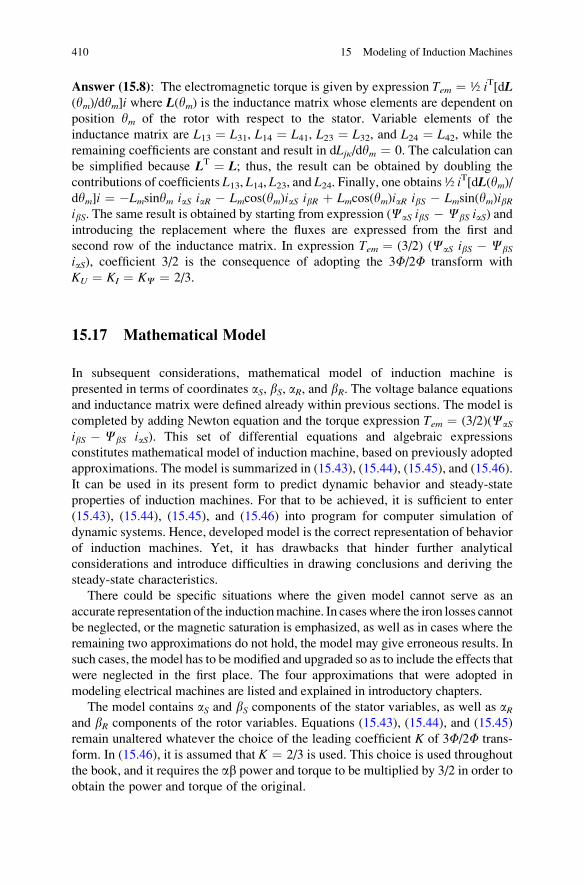
Answer (15.8): The electromagnetic torque is given by expression Tem ¼ ½ iT[dL(ym)/dym]i where L(ym) is the inductance matrix whose elements are dependent on
position ym of the rotor with respect to the stator. Variable elements of the
inductance matrix are L13 ¼ L31, L14 ¼ L41, L23 ¼ L32, and L24 ¼ L42, while the
remaining coefficients are constant and result in dLјк/dym ¼ 0. The calculation can
be simplified because LT ¼ L; thus, the result can be obtained by doubling the
contributions of coefficients L13, L14, L23, and L24. Finally, one obtains ½ iT[dL(ym)/dym]i ¼ �Lmsinym iaS iaR � Lmcos(ym)iaS ibR þ Lmcos(ym)iaR ibS � Lmsin(ym)ibRibS. The same result is obtained by starting from expression (CaS ibS � CbS iaS) andintroducing the replacement where the fluxes are expressed from the first and
second row of the inductance matrix. In expression Tem ¼ (3/2) (CaS ibS � CbS
iaS), coefficient 3/2 is the consequence of adopting the 3F/2F transform with
KU ¼ KI ¼ KC ¼ 2/3.
15.17 Mathematical Model
In subsequent considerations, mathematical model of induction machine is
presented in terms of coordinates aS, bS, aR, and bR. The voltage balance equationsand inductance matrix were defined already within previous sections. The model is
completed by adding Newton equation and the torque expression Tem ¼ (3/2)(CaS
ibS � CbS iaS). This set of differential equations and algebraic expressions
constitutes mathematical model of induction machine, based on previously adopted
approximations. The model is summarized in (15.43), (15.44), (15.45), and (15.46).
It can be used in its present form to predict dynamic behavior and steady-state
properties of induction machines. For that to be achieved, it is sufficient to enter
(15.43), (15.44), (15.45), and (15.46) into program for computer simulation of
dynamic systems. Hence, developed model is the correct representation of behavior
of induction machines. Yet, it has drawbacks that hinder further analytical
considerations and introduce difficulties in drawing conclusions and deriving the
steady-state characteristics.
There could be specific situations where the given model cannot serve as an
accurate representation of the inductionmachine. In caseswhere the iron losses cannot
be neglected, or the magnetic saturation is emphasized, as well as in cases where the
remaining two approximations do not hold, the model may give erroneous results. In
such cases, the model has to be modified and upgraded so as to include the effects that
were neglected in the first place. The four approximations that were adopted in
modeling electrical machines are listed and explained in introductory chapters.
The model contains aS and bS components of the stator variables, as well as aRand bR components of the rotor variables. Equations (15.43), (15.44), and (15.45)
remain unaltered whatever the choice of the leading coefficient K of 3F/2F trans-
form. In (15.46), it is assumed that K ¼ 2/3 is used. This choice is used throughout
the book, and it requires the ab power and torque to be multiplied by 3/2 in order to
obtain the power and torque of the original.
410 15 Modeling of Induction Machines
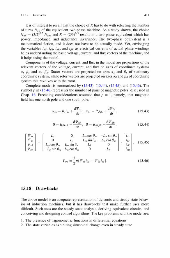
It is of interest to recall that the choice of K has to do with selecting the number
of turns Nab of the equivalent two-phase machine. As already shown, the choice
Nab ¼ (3/2)0.5 Nabc and K ¼ (2/3)0.5 results in a two-phase equivalent which has
power, impedance, and inductance invariance. The two-phase equivalent is a
mathematical fiction, and it does not have to be actually made. Yet, envisaging
the variables iaS, ibS, iaR, and ibR as electrical currents of actual phase windings
helps understanding the basic voltage, current, and flux vectors of the machine, and
it helps using the model.
Components of the voltage, current, and flux in the model are projections of the
relevant vectors of the voltage, current, and flux on axes of coordinate systems
aS–bS and aR–bR. Stator vectors are projected on axes aS and bS of stationary
coordinate system, while rotor vectors are projected on axes aR and bR of coordinatesystem that revolves with the rotor.
Complete model is summarized by (15.43), (15.44), (15.45), and (15.46). The
symbol p in (15.46) represents the number of pairs of magnetic poles, discussed in
Chap. 16. Preceding considerations assumed that p ¼ 1, namely, that magnetic
field has one north pole and one south pole:
uas ¼ Rsias þ dCas
dt; ubs ¼ Rsibs þ dCbs
dt; (15.43)
0 ¼ RRiaR þ dCaR
dt; 0 ¼ RRibR þ dCbR
dt; (15.44)
Cas
Cbs
CaR
CbR
2664
3775 ¼
Ls 0 Lm cos ym �Lm sin ym0 Ls Lm sin ym Lm cos ym
Lm cos ym Lm sin ym LR 0
�Lm sin ym Lm cos ym 0 LR
2664
3775 �
iasibsiaRibR
2664
3775; (15.45)
Tem ¼ 3
2p CaSibS �CbSiaS�
: (15.46)
15.18 Drawbacks
The above model is an adequate representation of dynamic and steady-state behav-
ior of induction machines, but it has drawbacks that make further uses more
difficult. Such uses are the steady-state analysis, deriving equivalent circuits, and
conceiving and designing control algorithms. The key problems with the model are:
1. The presence of trigonometric functions in differential equations
2. The state variables exhibiting sinusoidal change even in steady state
15.18 Drawbacks 411
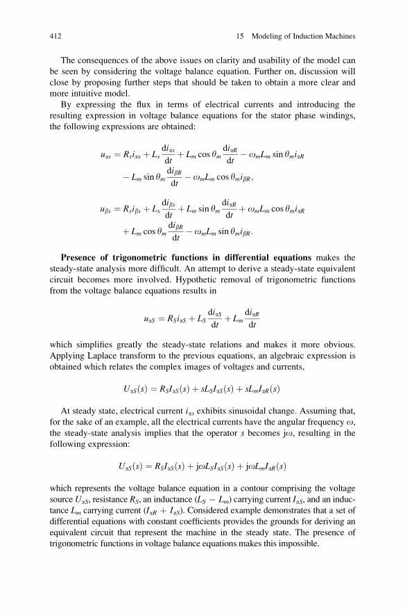
The consequences of the above issues on clarity and usability of the model can
be seen by considering the voltage balance equation. Further on, discussion will
close by proposing further steps that should be taken to obtain a more clear and
more intuitive model.
By expressing the flux in terms of electrical currents and introducing the
resulting expression in voltage balance equations for the stator phase windings,
the following expressions are obtained:
uas ¼ Rsias þ Lsdiasdt
þ Lm cos ymdiaRdt
� omLm sin ymiaR
� Lm sin ymdibRdt
� omLm cos ymibR;
ubs ¼ Rsibs þ Lsdibsdt
þ Lm sin ymdiaRdt
þ omLm cos ymiaR
þ Lm cos ymdibRdt
� omLm sin ymibR:
Presence of trigonometric functions in differential equations makes the
steady-state analysis more difficult. An attempt to derive a steady-state equivalent
circuit becomes more involved. Hypothetic removal of trigonometric functions
from the voltage balance equations results in
uaS ¼ RSiaS þ LSdiaSdt
þ LmdiaRdt
which simplifies greatly the steady-state relations and makes it more obvious.
Applying Laplace transform to the previous equations, an algebraic expression is
obtained which relates the complex images of voltages and currents,
UaSðsÞ ¼ RSIaSðsÞ þ sLSIaSðsÞ þ sLmIaRðsÞ
At steady state, electrical current ias exhibits sinusoidal change. Assuming that,
for the sake of an example, all the electrical currents have the angular frequency o,the steady-state analysis implies that the operator s becomes jo, resulting in the
following expression:
UaSðsÞ ¼ RSIaSðsÞ þ joLSIaSðsÞ þ joLmIaRðsÞ
which represents the voltage balance equation in a contour comprising the voltage
source UaS, resistance RS, an inductance (LS � Lm) carrying current IaS, and an induc-tance Lm carrying current (IaR þ IaS). Considered example demonstrates that a set of
differential equations with constant coefficients provides the grounds for deriving an
equivalent circuit that represent the machine in the steady state. The presence of
trigonometric functions in voltage balance equations makes this impossible.
412 15 Modeling of Induction Machines
Sinusoidal change of state variables even in steady-state conditions brings in
more difficulties in steady-state analysis. At the same time, similar difficulties are
encountered in designing control structures for the current, flux, and torque regula-
tion. The models with state variables that remain unaltered in the steady state are
simple to grasp. In their steady-state equations, all the time derivatives of the state
variables disappear, and the remaining expressions are easy to understand and use.
Yet, the present model does not have this possibility. The state variables of the
model, such as ias, exhibit sinusoidal changes even in the steady state.
Most mathematical models are usually formulated in such way that their state
variables remain constant in the steady state. The time derivatives of these state
variables are then equal to zero. In such cases, steady-state relations are obtained
from differential equations by removing the time derivatives.
Perpetual changes of state variables even in steady state make the control
problems more difficult to solve. An example to that is the applications of electrical
motors in industrial robots or autonomous vehicles, where the electrical motors are
used for controlling the motion. For that to be achieved, it is necessary to regulatesome relevant motor variables, such as the flux, torque, speed, and current. The term
regulation implies:
• Definition of a desired reference value for the controlled variable (such as the
phase current) that should be reached and maintained
• Measurement of the controlled variable (current) and calculation of the error,the deviation of the controlled variable from the desired value
• Performing control algorithm, calculation procedure or formula which receives
the error and calculates the control, the output of the control algorithm5
• Bringing the control variable to the system under control through an executiveorgan or actuator6
When the reference value does not change, the steady-state error can be reduced
to zero by adding integral control action into the control algorithm. Corresponding
control action is proportional to the integral of the error. Yet, this maintains the
error at zero only for constant references. In cases when the reference value has
perpetual changes, control actions would act upon the controlled variable to track
these changes. This is achieved at the cost of an error which cannot be removed.
5 By using devices called actuators or amplifiers, control output can affect the system and change the
controlled variable. Control algorithm is suited to reduce error and bring the controlled variable
toward the reference.Well-suited control algorithm ensures progressive reduction of the error which,
after a while, reaches zero. Hence, the steady-state value of errors is expected to be equal to zero.6 Control of phase currents of most electrical machines often includes switching power converters
employing power transistors and PWM techniques, as well as digital signal controllers. The
control algorithm is usually implemented by programming digital signal controllers. Control
variables are obtained in numerical form, as binary-coded digital words that reside within
processor registers. On the other side, the actual control variable that has the potential to change
the phase current is the voltage across the phase winding which may change within the range of
�600 V. The executive organ is often a switching transistor which receives gating signals from the
digital signal controller.
15.18 Drawbacks 413
Namely, controlled variable would track the reference with a tracking error that
depends on the rate of change of the reference. The presence of error can jeopardize
the operation of the whole system.
Induction machines have alternating currents in their phase windings. Hence,
even in the steady state, the variables ias and ibs exhibit sinusoidal changes.
Whenever there is a need to regulate stator currents of induction machine, con-
trolled variables are variable even at steady state. This creates the need to transform
the mathematical model in such way that the steady-state values of the state
variables are constant and to use this model to formulate the control algorithm.
Question (15.9): Is there an operating mode of an induction machine where the
frequency of stator currents is zero?
Answer (15.9): Considering induction machines supplied from constant frequency
voltage sources, the frequency of the stator electrical currents is determined by the
frequency of voltages fed to the stator winding. If induction machine is connected to
the mains, the frequency of the stator current will be 50 Hz, irrespective of the rotor
speed, torque, or power. For that reason, the stator currents may have different
frequency only in cases when the induction machine is supplied from a variable
frequency, variable voltage source such as the static power converter which uses
semiconductor power switches and operates on pulse-width modulation principles.
In this way, the stator winding can be supplied with a symmetrical system of three-
phase voltages of variable amplitude and variable frequency.
In further considerations, it is assumed that the supply voltage has variable
frequency oe which can be adjusted to achieve desired operating mode. For two-
pole machine, oe ¼ Om þ oslip, where Om is the rotor speed while oslip is the slip
frequency. Operating mode where DC current flows through the stator is the one
where Om ¼ �oslip, resulting in oe ¼ 0. It should be noted that the slip frequency
is proportional to the developed electromagnetic torque. Therefore, the operating
mode with oe ¼ 0 is reached when the torque and speed of rotation are of different
signs. The rotor rotates at the speed which has the same magnitude as the slip
frequency, but it has opposite sign. In one of such cases, the motor is stopped and
develops the torque Tem ¼ 0. In another example, the rotor revolves at�300 rpm, it
develops positive torque, and it has the rotor currents of 5 Hz.
15.19 Model in Synchronous Coordinate Frame
The problems of analysis and control based onmathematical model in a–b coordinate
frame arise due to the fact that the state variables exhibit sinusoidal change even in
the steady state. Namely, projections of the vectors of currents, voltages, and flux
linkages on the axes of a–b coordinate frame change as sinusoidal functions even in
steady state, with constant amplitude of magnetomotive force FS, constant flux, and
constant rotor speed. This deficiency of the model can be removed by applying
another transform of the state coordinates and replacing the existing state variables
414 15 Modeling of Induction Machines
by the new ones. The new variables should be selected so that their values at steady
state do not vary. The new coordinate transform should maintain the invariability in
terms of impedance, inductance, and power. For that to be achieved, the same
transformation matrix should be applied to all the variables, whether the currents,
voltages, or flux linkages. The question arises about how to devise this new coordi-
nate transform.
15.20 Park Transform
In the model of the machine which is formulated in stationary a–b frame, the stator
currents iaS and ibS are projections of the vector of magnetomotive force FS ¼ NS iSon axes of the aS–bS coordinate system. The problem arises due to the fact that FS is
a rotating vector. Its rotation with respect to a–b frame makes the projections iaSand ibS variable. In steady state, they become sinusoidal function. In order to solve
the problem, it is necessary to envisage a new coordinate system which is rotating at
the same speed as the magnetomotive force FS. In this case, projections of this
vector on new pair of axes do not change in the steady state, as the relative position
between the revolving vector and the new frame does not change. The same
conclusion applies for the voltage and flux vectors. Therefore, the new transform
of the state coordinates should formulate the model of induction machine in a new
coordinate system which revolves synchronously with the field.
By adopting a synchronously rotating coordinate system having axes d and q,projections id and iq of the stator current vector iS ¼ FS/NS on these new axes have
constant steady-state values. Therefore, by transforming all the stator quantities
from the stationary aS–bS coordinate system to the synchronously rotating d–qcoordinate system, a model of the stator winding is obtained where the relevant
quantities have constant steady-state values.
Transform implies a relation that expresses the variables of the d–q system
(id and iq) in terms of the variables of the aS–bS coordinate system (iaS and ibS).Applying a coordinate transform does not introduce any change to the considered
induction machine nor to its flux or torque. The transform merely represents a
different point of view and represents one and the same actual systems by means of
another mathematical representation. Therefore, no matter whether the mathemati-
cal model is formulated in the stationary or in the synchronous coordinate frame, it
must describe the same vectors of the magnetomotive force, flux, voltage, and
current as well as the same torque, speed, and power of electromechanical conver-
sion. Consequently, both the model in a–b frame and the model in d–q frame must
have one and the same vector of the stator magnetomotive force FS. In other words,
the vector FS created by currents iaS and ibS must have the same amplitude and
spatial orientation as the vector FS created by id and iq, the stator currents
transformed into d–q coordinate frame.
Coordinate transform is essentially a mathematical operation, and it does not
have to result in state variables that correspond to an actual, physical machine.
15.20 Park Transform 415
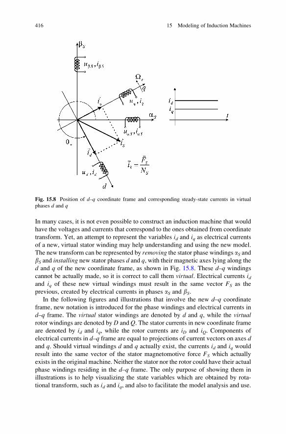
In many cases, it is not even possible to construct an induction machine that would
have the voltages and currents that correspond to the ones obtained from coordinate
transform. Yet, an attempt to represent the variables id and iq as electrical currentsof a new, virtual stator winding may help understanding and using the new model.
The new transform can be represented by removing the stator phase windings aS andbS and installing new stator phases d and q, with their magnetic axes lying along the
d and q of the new coordinate frame, as shown in Fig. 15.8. These d–q windings
cannot be actually made, so it is correct to call them virtual. Electrical currents idand iq of these new virtual windings must result in the same vector FS as the
previous, created by electrical currents in phases aS and bS.In the following figures and illustrations that involve the new d–q coordinate
frame, new notation is introduced for the phase windings and electrical currents in
d–q frame. The virtual stator windings are denoted by d and q, while the virtualrotor windings are denoted by D and Q. The stator currents in new coordinate frame
are denoted by id and iq, while the rotor currents are iD and iQ. Components of
electrical currents in d–q frame are equal to projections of current vectors on axes dand q. Should virtual windings d and q actually exist, the currents id and iq wouldresult into the same vector of the stator magnetomotive force FS which actually
exists in the original machine. Neither the stator nor the rotor could have their actual
phase windings residing in the d–q frame. The only purpose of showing them in
illustrations is to help visualizing the state variables which are obtained by rota-
tional transform, such as id and iq, and also to facilitate the model analysis and use.
Fig. 15.8 Position of d–q coordinate frame and corresponding steady-state currents in virtual
phases d and q
416 15 Modeling of Induction Machines
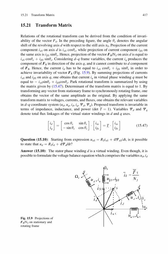
15.21 Transform Matrix
Relations of the rotational transform can be derived from the condition of invari-
ability of the vector FS. In the preceding figure, the angle ye denotes the angular
shift of the revolving axis d with respect to the still axis aS. Projection of the currentcomponent iaS on axis d is iaS cosye, while projection of current component ibS onthe same axis is ibS sinye. Hence, projection of the vector FS/NS on axis d is equal toiaS cosye þ ibS sinye. Considering d–q frame variables, the current iq produces thecomponent of FS in direction of the axis q, and it cannot contribute to d component
of FS. Hence, the current id has to be equal to iaS cosye þ ibS sinye in order to
achieve invariability of vector FS (Fig. 15.9). By summing projections of currents
iaS and ibS on axis q, one obtains that current iq in virtual phase winding q must be
equal to � iaSsinye þ ibScosye. Park rotational transform is summarized by using
the matrix given by (15.47). Determinant of the transform matrix is equal to 1. By
transforming any vector from stationary frame to synchronously rotating frame, one
obtains the vector of the same amplitude as the original. By applying the same
transform matrix to voltages, currents, and fluxes, one obtains the relevant variables
in d–q coordinate system (ud, uq, id, iq,Cd,Cq). Proposed transform is invariable in
terms of impedance, inductance, and power (det T ¼ 1). Variables Cd and Cq
denote total flux linkages of the virtual stator windings in d and q axes.
idiq
� �¼ cos ys sin ys
� sin ys cos ys
� �� ias
ibs
� �¼ T � ias
ibs
� �(15.47)
Question (15.10): Starting from expression uaS ¼ RSiaS þ dCaS/dt, is it possibleto state that ud ¼ RSid þ dCd/dt?
Answer (15.10): The stator phase winding d is a virtual winding. Even though, it is
possible to formulate the voltage balance equationwhich comprises the variables ud, id
Fig. 15.9 Projections of
FS/NS on stationary and
rotating frame
15.21 Transform Matrix 417
and other variables of the d–q frame. The presence of unchanged stator resistanceRS is
expected since the transform is invariant in terms of impedance. However, it cannot be
stated that ud ¼ RSid þ dCd/dt. Namely, the voltage balance equation u ¼ Ri þ dC/
dt applies to any winding that actually exists or the winding that could actually be
made. Relation u ¼ Ri þ dC/dt was used to model the voltage balance in aS–bScoordinate frame. Although the original induction machine has three phases, the two-
phase stator winding in aS–bS frame can be actually made. Therefore, the stator phase
windings aS and bS can be considered as real windings. Thus, the voltage balance
equation in aS–bS frame is u ¼ Ri þ dC/dt. On the other hand, the phase windings indq frame cannot bemade. The analysis performed later on proves that the voltage ud isnot equal to RSid þ dCd/dt. The actual voltage balance equations in dq frame,
describing the virtual voltages, will be derived by applying the transform matrix to
equations uaS ¼ RSiaS þ dCaS/dt and ubS ¼ RSibS þ dCbS/dt.
15.22 Transforming Rotor Variables
It is beneficial to have both the stator and the rotor variables residing in the same
frame of coordinates. For that to be achieved, it is necessary to apply rotational
transform to the rotor variables and find their DQ equivalents.
Park transform of the stator phase windings aS and bS results in two virtual statorphases in dq frame. In the same way, it is necessary to replace the short-circuited
rotor cage by two virtual rotor phases residing in d–q coordinate system. For clarity,
notation adopted hereafter implies that the stator variables have lower case
subscripts dq, while the rotor variables have upper case subscripts DQ.It is necessary to explain the need for transforming the stator and rotor variables to
the same, synchronously rotating, coordinate system. First of all, it should be recalled
that the voltage balance equations in stationary a–b coordinate frame are difficult to
cope with due to variable coefficients of differential equations. These variable
coefficients come from variable elements in the inductance matrix, such as L13 ¼Lmcos(ym). Some mutual inductances between stator and rotor phases are variable
(15.48) due to change in relative position of the twowindings. In (15.45), this comes as
a consequence of the aR–bR framemovingwith respect to the aS–bS frame. Themutual
inductance between the two windings does not change as long as they maintain the
same relative position. Hence, any pair of windings residing in the same coordinate
frame, whether revolving or stationary, does not change relative position, and there-
fore, they have constant mutual inductance. Transformation of rotor windings from
aRbR frame to d–q coordinate frame can be depicted as removing the original aRbRwindings and replacing them with a pair of virtual rotor phases denoted by DQ,residing in the same d–q coordinate frame as the virtual stator phases denoted by dq.Now the stator dq windings do not move with respect to the rotor DQ windings.
Therefore, all the self-inductances and all the mutual inductances are constant. The
inductance matrix that corresponds to virtual windings in dq frame has constant
418 15 Modeling of Induction Machines
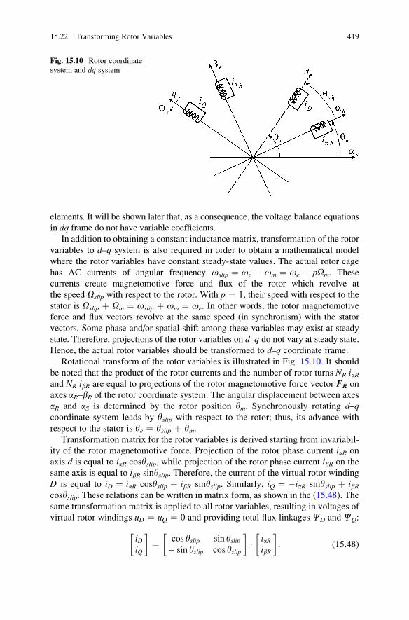
elements. It will be shown later that, as a consequence, the voltage balance equations
in dq frame do not have variable coefficients.
In addition to obtaining a constant inductance matrix, transformation of the rotor
variables to d–q system is also required in order to obtain a mathematical model
where the rotor variables have constant steady-state values. The actual rotor cage
has AC currents of angular frequency oslip ¼ oe � om ¼ oe � pOm. These
currents create magnetomotive force and flux of the rotor which revolve at
the speed Oslip with respect to the rotor. With p ¼ 1, their speed with respect to the
stator is Oslip þ Om ¼ oslip þ om ¼ oe. In other words, the rotor magnetomotive
force and flux vectors revolve at the same speed (in synchronism) with the stator
vectors. Some phase and/or spatial shift among these variables may exist at steady
state. Therefore, projections of the rotor variables on d–q do not vary at steady state.Hence, the actual rotor variables should be transformed to d–q coordinate frame.
Rotational transform of the rotor variables is illustrated in Fig. 15.10. It should
be noted that the product of the rotor currents and the number of rotor turns NR iaRand NR ibR are equal to projections of the rotor magnetomotive force vector FR on
axes aR–bR of the rotor coordinate system. The angular displacement between axes
aR and aS is determined by the rotor position ym. Synchronously rotating d–qcoordinate system leads by yslip with respect to the rotor; thus, its advance with
respect to the stator is ye ¼ yslip þ ym.Transformation matrix for the rotor variables is derived starting from invariabil-
ity of the rotor magnetomotive force. Projection of the rotor phase current iaR on
axis d is equal to iaR cosyslip, while projection of the rotor phase current ibR on the
same axis is equal to ibR sinyslip. Therefore, the current of the virtual rotor windingD is equal to iD ¼ iaR cosyslip þ ibR sinyslip. Similarly, iQ ¼ �iaR sinyslip þ ibRcosyslip. These relations can be written in matrix form, as shown in the (15.48). The
same transformation matrix is applied to all rotor variables, resulting in voltages of
virtual rotor windings uD ¼ uQ ¼ 0 and providing total flux linkages CD and CQ:
iDiQ
� �¼ cos yslip sin yslip
� sin yslip cos yslip
� �� iaR
ibR
� �: (15.48)
Fig. 15.10 Rotor coordinate
system and dq system
15.22 Transforming Rotor Variables 419
15.23 Vectors and Complex Numbers
Park transform relates coordinates of vectors in a–b coordinate system to
coordinates of the same vectors in d–q coordinate system. All the voltages, currents,
magnetomotive forces, and fluxes can be represented by vectors, either in ab frame
or in dq frame. All the vectors have two components, being associated with two-
phase windings. Projection of each voltage, current, or flux vector on one of the
axes corresponds to voltage, current, or flux linkage in the phase winding residing
on corresponding axis.
With all the vectors residing in plane, it is possible to use complex notation in
representing individual vectors. Namely, a vector can be represented by a complex
number, with real and imaginary parts representing the projections of the vector on
the two orthogonal axes. In this way, Park transform notation can be simplified, and
the transformation matrix reduced to a complex number. As an example, the vector
of the stator current can be expressed in terms of its aS component, directed along aSaxis, and its bS component, directed along bS axis. If aS axis is given attributes of thereal axis and axis bS attributes of the imaginary axis, the aS–bS plane is interpretedas the complex plane, where the current vector is represented by complex number,
~iabS ¼~a0iaS þ~b0ibS ) iabS ¼ iaS þ j ibS:
Similarly, considering the current vector in d–q system, axis d can be given
attributes of the real axis, while axis q can be treated as imaginary axis, converting
in this way d–q space into a complex plane, where the current is represented by the
complex number idq ¼ id þ jiq. Complex notation of current vectors is not unique.
With axis d as real axis, the number idq is obtained, different than the complex
number iab obtained with axis aS as real axis.
15.23.1 Simplified Record of the Rotational Transform
By using the complex notation, Park transform can be written as
idq ¼ id þ jiq ¼ iabSe�j ye ;
iabSe�j ye ¼ iaS þ j ibS
� cos yeð Þ � j sin yeð Þð Þ
¼ ðiaS cos yeð Þ þ ibS sin yeð Þ Þ þ j �iaS sin yeð Þ þ ibS cos yeð Þ� :
The inverse transform can be written as
iabS ¼ idqeþjye :
420 15 Modeling of Induction Machines
Complex number idq ¼ id þ jiq is a compact way of representing the stator
current vector by representing the two state variables, id and iq, as a single complex
number. The choice of real axis (d) and complex axis (q) is in accordance with the
fact that axis q leads by p/2 and that imaginary unit j ¼ exp(jp/2) represents thephase shift of p/2. Complex notation idq acquires another significance in steady
state. With id and iq remaining constant, the steady-state value of idq becomes a
complex constant, phasor. The amplitude and argument of this phasor determine
the amplitude and the initial phase of the stator current.
15.24 Inductance Matrix in dq Frame
By application of Park transform, the rotor and stator windings are transferred to
synchronously rotating d–q system. The virtual stator windings are denoted by
subscripts d and q, while virtual rotor windings are denoted by subscripts D and Q.Rotation of dq frame does not change relative position of stator and rotor virtual
phases; thus, all coefficients of relevant inductance matrix remain constant. The
flux of the stator winding d is determined by the first row of matrix, Cd ¼ LSid þLmiD. The mutual inductance is constant since windings d andD do not change their
relative positions.
Revolving frame has an angular speed Oe which is the same as the speed of the
revolving field. The speed Oe is determined by the angular frequency of stator
voltages and currents, oe. For two-pole machines with p ¼ 1, Oe ¼ oe. The angle
between axes d and aS is equal to
ye ¼ yeð0Þ þðt
0
Oedt: (15.49)
Stator currents are
idiq
� �¼ cos ye sin ye
� sin ye cos ye
� �� ias
ibs
� �: (15.50)
Complex notation of the stator current is
idq ¼ id þ jiq ¼ e�jye iab: (15.51)
Rotor currents are
iDiQ
� �¼ cos yslip sin yslip
� sin yslip cos yslip
� �� iaR
ibR
� �: (15.52)
15.24 Inductance Matrix in dq Frame 421
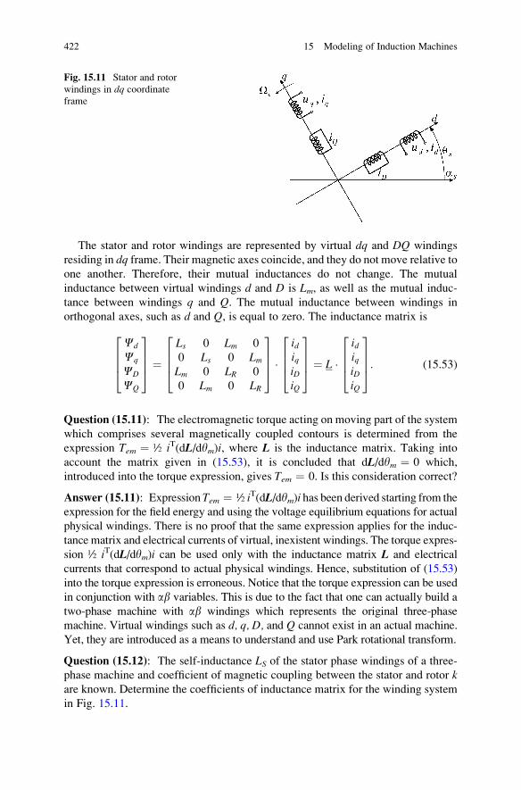
The stator and rotor windings are represented by virtual dq and DQ windings
residing in dq frame. Their magnetic axes coincide, and they do not move relative to
one another. Therefore, their mutual inductances do not change. The mutual
inductance between virtual windings d and D is Lm, as well as the mutual induc-
tance between windings q and Q. The mutual inductance between windings in
orthogonal axes, such as d and Q, is equal to zero. The inductance matrix is
Cd
Cq
CD
CQ
2664
3775 ¼
Ls 0 Lm 0
0 Ls 0 LmLm 0 LR 0
0 Lm 0 LR
2664
3775 �
idiqiDiQ
2664
3775 ¼ L �
idiqiDiQ
2664
3775: (15.53)
Question (15.11): The electromagnetic torque acting on moving part of the system
which comprises several magnetically coupled contours is determined from the
expression Tem ¼ ½ iT(dL/dym)i, where L is the inductance matrix. Taking into
account the matrix given in (15.53), it is concluded that dL/dym ¼ 0 which,
introduced into the torque expression, gives Tem ¼ 0. Is this consideration correct?
Answer (15.11): Expression Tem ¼ ½ iT(dL/dym)i has been derived starting from the
expression for the field energy and using the voltage equilibrium equations for actual
physical windings. There is no proof that the same expression applies for the induc-
tance matrix and electrical currents of virtual, inexistent windings. The torque expres-
sion ½ iT(dL/dym)i can be used only with the inductance matrix L and electrical
currents that correspond to actual physical windings. Hence, substitution of (15.53)
into the torque expression is erroneous. Notice that the torque expression can be used
in conjunction with ab variables. This is due to the fact that one can actually build a
two-phase machine with ab windings which represents the original three-phase
machine. Virtual windings such as d, q, D, and Q cannot exist in an actual machine.
Yet, they are introduced as a means to understand and use Park rotational transform.
Question (15.12): The self-inductance LS of the stator phase windings of a three-phase machine and coefficient of magnetic coupling between the stator and rotor kare known. Determine the coefficients of inductance matrix for the winding system
in Fig. 15.11.
Fig. 15.11 Stator and rotor
windings in dq coordinate
frame
422 15 Modeling of Induction Machines
Answer (15.12): The inductance matrix in (15.53) is obtained by applying Clarke
3F/2F transform to the original three-phase machine and then applying Park
rotational transform to the two-phase ab equivalent. The applied transforms are
invariant in terms of inductance. Therefore, elements L11 and L22 of the matrix are
equal to LS. Considering the rotor model, it is usually assumed that the short-
circuited rotor winding has the same number of turns as the stator and that magnetic
resistance along paths of the two fluxes is approximately equal; thus, LS ¼ LR. Thecoefficients of mutual inductance are equal to Lm ¼ k(LSLR)
0.5 ¼ kLS.Successive application of Clarke and Park transforms results in the transform
known as Blondel transform.
15.25 Voltage Balance Equations in dq Frame
Mathematical model of the electrical subsystem comprises the voltage balance
equations, differential equations that express the equilibrium of the supply voltage,
the voltage drops, and electromotive forces in actual phase windings. These
equations can be transformed from ab frame to dq frame, synchronous with the
revolving field. In ab stationary coordinate system, voltage equilibrium in the stator
phase windings is given by
uaS ¼ RSiaS þ dCaS=dt; ubS ¼ RSibS þ dCbS=dt: (15.54)
Multiplication of the second equation by j and summing the two equations result
in a single voltage balance equation with voltages, fluxes, and currents expressed as
complex numbers,
uabS ¼ uaS þ jubS� ¼ RS iaS þ jibS
� þ d CaS þ jCbS�
=dt
¼ RSiabS þ dCabS=dt: (15.55)
Voltages of virtual d-phase and q-phase windings are obtained from ab voltages
by applying Park transform,
udq ¼ ud þ juq ¼ uabSe�jye ¼ RSiabS þ dCabS=dt
�e�jye : (15.56)
Variables iabS and CabS of the stationary coordinate system can be represented in
termsofdqvariables by applying inversePark transform, iabS ¼ idqexp(�jye), to obtain
udq ¼ RSidqeþjye þ d Cdqe
þjye�
=dt �
e�jye
¼ RSidq þ dCdq=dtþ joeCdq: (15.57)
15.25 Voltage Balance Equations in dq Frame 423
Therefore, voltage balance equations of virtual stator phases in dq frame do not
have the form u ¼ Ri þ dC/dt. They contain an additional member which comes
as a consequence of Park transform. The above equation with complex numbers can
be separated into real and imaginary parts, resulting in two scalar equations. The
same procedure can be applied to the voltage balance equations of the rotor
windings, but this time the angle ye is replaced by angle yslip. This is due to the
fact that the angle between the original rotor coordinate system (aR–bR) and the
target dq coordinate system is yslip ¼ ye � ym. For the virtual rotor windings (DQ),the following voltage balance equations are obtained:
uDQ ¼ RRiDQeþjyslip þ d CDQe
þjyslip�
=dt �
e�jyslip
¼ RRiDQ þ dCDQ=dtþ joslipCDQ: (15.58)
15.26 Electrical Subsystem
This section summarizes the model of the electrical subsystem of induction
machine expressed in synchronous dq frame, where the state variables are con-
stant in the steady state and where the inductance matrix of virtual windings has
constant elements. This model is based on the four approximations adopted in
modeling induction machines. They are detailed in introductory chapters, and
they include:
1. Neglected effects of distributed parameters.
2. The energy of electrical field is neglected along with parasitic capacitances.
3. Neglected are the iron losses.
4. Magnetic saturation is neglected along with nonlinear B(H) characteristic of
ferromagnetic materials.
Moreover, the leading coefficient of Clarke transform, used to replace the three-
phase original with the two-phase equivalent, is K ¼ 2/3. For simplicity, further
considerations assume that the induction machine under consideration is two-pole
machine where p ¼ 1 and that electrical angular frequency o corresponds to
mechanical angular speed O, resulting in o ¼ pO.The following equations give complete mathematical model of the electrical
subsystem of an induction machine in the synchronously rotating dq coordinate
system. The two voltage balance equations with complex variables are split into
four voltage balance equations with scalars:
ud ¼ Rsid þ dCd
dt� oeCq; (15.59)
424 15 Modeling of Induction Machines
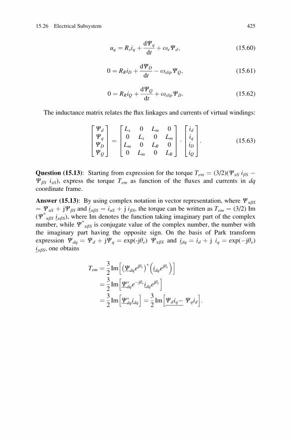
uq ¼ Rsiq þ dCq
dtþ oeCd; (15.60)
0 ¼ RRiD þ dCD
dt� oslipCQ; (15.61)
0 ¼ RRiQ þ dCQ
dtþ oslipCD: (15.62)
The inductance matrix relates the flux linkages and currents of virtual windings:
Cd
Cq
CD
CQ
2664
3775 ¼
Ls 0 Lm 0
0 Ls 0 LmLm 0 LR 0
0 Lm 0 LR
2664
3775 �
idiqiDiQ
2664
3775: (15.63)
Question (15.13): Starting from expression for the torque Tem ¼ (3/2)(CaS ibS �CbS iaS), express the torque Tem as function of the fluxes and currents in dqcoordinate frame.
Answer (15.13): By using complex notation in vector representation, where CabS
¼ CaS þ jCbS and iabS ¼ iaS þ j ibS, the torque can be written as Tem ¼ (3/2) Im
(C*abS iabS), where Im denotes the function taking imaginary part of the complex
number, while C*abS is conjugate value of the complex number, the number with
the imaginary part having the opposite sign. On the basis of Park transform
expression Cdq ¼ Cd þ jCq ¼ exp(-jye) CabS and idq ¼ id þ j iq ¼ exp(�jye)iabS, one obtains
Tem ¼ 3
2Im Cdqe
jye�
idqejye
�h i
¼ 3
2Im C
dqe�jye idqe
jyeh i
¼ 3
2Im C
dqidq
h i¼ 3
2Im Cdiq� Cqid
h i:
15.26 Electrical Subsystem 425
Chapter 16
Induction Machines at Steady State
In this chapter, steady state operation of induction machines is studied with the aim
to derive the equivalent circuit and mechanical characteristic of induction machine.
The steady state model is derived from the dynamic model, developed and
explained in the previous chapter. The voltage balance equations at steady state
are used to develop the steady state equivalent circuit of the machine with squirrel
cage rotor. At the same time, the concept of the equivalent transformer is introduced
to derive the same steady state equivalent circuit. The equivalent circuit is used to
determine the steady state currents, torque, power, losses, and flux linkages. Typical
resistances and inductances of the equivalent circuit are explained and discussed,
along with typical experimental procedures for their measurement and estimation.
The system of relative units is introduced and explained, along with benefits that
come from its use. Characteristic examples are studied to develop skills in working
with relative units and selecting the base quantities used in scaling the absolute
values into relative values. The functions that approximate the mechanical charac-
teristic of induction machine and typical mechanical loads are introduced and
explained. Natural mechanical characteristic is analyzed along with the start-up
mode, rated operation, and no load operation. Breakdown torque is studied and
explained in both motor and generator modes. Stable and unstable equilibrium
points on mechanical characteristic are discussed and explained. The influence of
machine resistances and reactances on the start-up torque, breakdown torque,
breakdown slip, and coefficient of efficiency is analyzed and explained. This
chapter proceeds by summarizing energy losses in windings, magnetic circuits,
and mechanical losses due to rotation. Calculation of steady state losses is
explained on the basis of the steady state equivalent circuit. The losses are
presented in the form of power balance chart drawn for induction machine that
operates in motoring mode. Simplified power balance is derived by splitting the air-
gap power into rotor losses and mechanical power, according to the relative slip s.This chapter ends with deriving power balance chart for induction generator and
discussing generator operating mode of induction machines.
S.N. Vukosavic, Electrical Machines, Power Electronics and Power Systems,
DOI 10.1007/978-1-4614-0400-2_16, # Springer Science+Business Media New York 2013
427
16.1 Input Power
Induction machines have short-circuited cage winding on the rotor, and they have
three-phase stator winding. The stator winding is supplied from the source of three-
phase voltages: ua, ub and uc. No electrical power is supplied through the rotor
winding. Electrical power supplied through the stator windings is pe ¼ uaia þ ubibþ ucic. Using Clarke transform, three-phase machine is replaced by two-phase
equivalent. With Clarke transform coefficient K ¼ 2/3, the input power to the
machine is equal to
pe ¼ 3
2uaSiaS þ ubSibS� �
¼ 3
2Re uaS þ jubS� �
iaS � jibS� �� � ¼ 3
2Re uabS
� �iabS
� ��h i:
By using Park transform, aS and bS phase windings are replaced by virtual d andq windings in synchronous coordinate frame. With idq ¼ exp(�jye) iabS and udq ¼exp(�jye) uabS, the input power can be expressed in terms of dq voltages and
currents:
pe ¼ 3
2Re uabS
� �iabS
� ��h i¼ 3
2Re udqe
jye� �
idqejye
� ��h i
¼ 3
2Re udqe
jye idq
� ��e�jye
h i¼ 3
2Re udq idq
� ��h i¼ 3
2udid þ uqiq� �
:
Starting from expression pe ¼ (3/2)(udid þ uqiq) for power delivered to the
machine from the electrical source, it is possible to calculate components of the
input power and determine the electromagnetic torque. By using voltage balance
equations for the stator winding, one obtains the source power pe as
pe ¼ 3
2udid þ uqiq� �
¼ 3
2Rs i2d þ i2q
� �þ 3
2
dCd
dtid þ dCq
dtiq
� þ 3
2oe Cdiq �Cqid� �
¼ pCu1 þ dWm
dtþ pd:
Component pcu1 represents losses in copper of the stator winding. Component
dWm/dt has dimension of power and represents the rate of change of the energy
accumulated in magnetic field, the first derivative of the field energy. During the
operation of induction machine, the air-gap flux may change its value. Therefore,
the instantaneous value of dWm/dt is positive when the flux increases and negative
when the flux decreases. The average value of dWm/dt must be equal to zero, since
the accumulated energy cannot increase indefinitely nor can it decrease indefinitely.
428 16 Induction Machines at Steady State
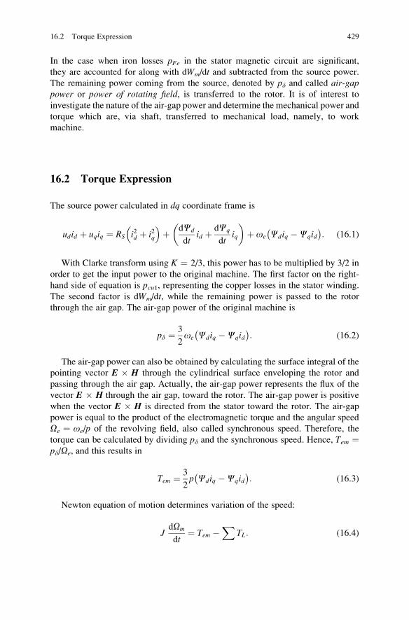
In the case when iron losses pFe in the stator magnetic circuit are significant,
they are accounted for along with dWm/dt and subtracted from the source power.
The remaining power coming from the source, denoted by pd and called air-gappower or power of rotating field, is transferred to the rotor. It is of interest to
investigate the nature of the air-gap power and determine the mechanical power and
torque which are, via shaft, transferred to mechanical load, namely, to work
machine.
16.2 Torque Expression
The source power calculated in dq coordinate frame is
udid þ uqiq ¼ RS i2d þ i2q
� �þ dCd
dtid þ dCq
dtiq
� þ oe Cdiq �Cqid
� �: (16.1)
With Clarke transform using K ¼ 2/3, this power has to be multiplied by 3/2 in
order to get the input power to the original machine. The first factor on the right-
hand side of equation is pcu1, representing the copper losses in the stator winding.
The second factor is dWm/dt, while the remaining power is passed to the rotor
through the air gap. The air-gap power of the original machine is
pd ¼ 3
2oe Cdiq �Cqid� �
: (16.2)
The air-gap power can also be obtained by calculating the surface integral of the
pointing vector E � H through the cylindrical surface enveloping the rotor and
passing through the air gap. Actually, the air-gap power represents the flux of the
vector E � H through the air gap, toward the rotor. The air-gap power is positive
when the vector E � H is directed from the stator toward the rotor. The air-gap
power is equal to the product of the electromagnetic torque and the angular speed
Oe ¼ oe/p of the revolving field, also called synchronous speed. Therefore, the
torque can be calculated by dividing pd and the synchronous speed. Hence, Tem ¼pd/Oe, and this results in
Tem ¼ 3
2p Cdiq �Cqid� �
: (16.3)
Newton equation of motion determines variation of the speed:
JdOm
dt¼ Tem �
XTL: (16.4)
16.2 Torque Expression 429
16.3 Relative Slip
If the rotor of an induction machine rotates at the speed of Om 6¼ Oe, different than
the synchronous speedOe, which determines the angular speed of the magnetic field,
then the slip speed is Oslip ¼ Oe � Om. The rotor speed changes during transients
and represents one of the state variables. At steady state, the rotor revolves at a
constant speed. The slip speed Oslip determines the angular frequency of the rotor
currents,oslip ¼ pOslip. The ratio s ¼ oslip/oe ¼ Oslip/Oe is called relative slip. Fora two-pole motor fed from the mains with the line frequency of 50 Hz, the synchro-
nous speed is 50 rev/s or 3,000 rpm (revolutions per minute). If the rotor revolves at
2,700 rpm, the relative slip is s ¼ 300/3,000 ¼ 0.1. For inductionmotor with locked
rotor (the rotor which does not rotate), relative slip is s ¼ 1.
16.4 Losses and Mechanical Power
Electromagnetic torque Tem acts on the rotor which revolves at the speed Om.
Related mechanical power pmR ¼ TemOm is also called internal mechanical
power. It is slightly different than the mechanical power pm ¼ TmOm transferred
to the external mechanical load via shaft. The difference between pmR ¼ TemOm
and pm ¼ TmOm appears due to internal mechanical losses within induction
machines. These losses are the air friction, friction in the bearings, and other losses
in mechanical subsystem of the machine. Therefore, electromagnetic torque Tem is
different than the torque Tm which is passed to the work machine through the shaft.
Detailed analysis of losses in induction machine is given in Sect. 16.24, along with
the balance of power which is shown in Fig. 16.17.
Mechanical power pmR differs from the air-gap power pd by the amount of losses
in rotor winding and rotor magnetic circuit. Electrical currents in rotor bars create
losses proportional to the square of the current, Ri2. Although the rotor bars are
usually made of aluminum, losses in the cage are frequently called copper lossesand denoted as PCu2. In addition to losses in the rotor windings, there are losses in
the rotor magnetic circuit, denoted by PFeR. Rotor magnetic circuit is, like that of
the stator, made of iron sheets. It contains magnetic field with sinusoidal change at
angular frequencyoslip, creating losses due to hysteresis and eddy currents. The slip
frequency oslip is much lower than the stator frequency oe; thus, it is justified to
neglect iron losses in the rotor. This approximation is not justified for operating
modes where the assumption oslip � oe does not hold, namely, where the relative
slip does not satisfy relation s � 1.
One example where the rotor iron losses cannot be neglected is the case of where
the induction motor with its rotor at standstill gets connected to the mains. This is
the most common way of starting mains supplied induction motors. With locked
rotor, Om ¼ 0 and s ¼ 1. The frequency of electrical currents in the rotor cage
corresponds to the line frequency as well as the frequency of changes of magnetic
induction B within the rotor magnetic circuit.
430 16 Induction Machines at Steady State
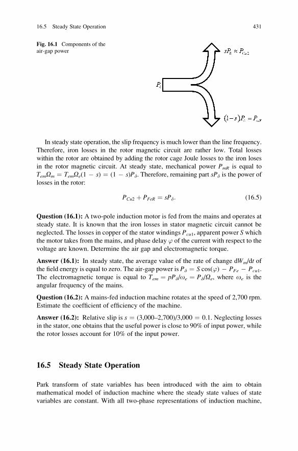
In steady state operation, the slip frequency is much lower than the line frequency.
Therefore, iron losses in the rotor magnetic circuit are rather low. Total losses
within the rotor are obtained by adding the rotor cage Joule losses to the iron loses
in the rotor magnetic circuit. At steady state, mechanical power PmR is equal to
TemOm ¼ TemOe(1 � s) ¼ (1 � s)Pd. Therefore, remaining part sPd is the power of
losses in the rotor:
PCu2 þ PFeR ¼ sPd: (16.5)
Question (16.1): A two-pole induction motor is fed from the mains and operates at
steady state. It is known that the iron losses in stator magnetic circuit cannot be
neglected. The losses in copper of the stator windings Pcu1, apparent power S whichthe motor takes from the mains, and phase delay ’ of the current with respect to the
voltage are known. Determine the air gap and electromagnetic torque.
Answer (16.1): In steady state, the average value of the rate of change dWm/dt ofthe field energy is equal to zero. The air-gap power is Pd ¼ S cos(’) � PFe � Pcu1.
The electromagnetic torque is equal to Tem ¼ pPd/oe ¼ Pd/Oe, where oe is the
angular frequency of the mains.
Question (16.2): A mains-fed induction machine rotates at the speed of 2,700 rpm.
Estimate the coefficient of efficiency of the machine.
Answer (16.2): Relative slip is s ¼ (3,000–2,700)/3,000 ¼ 0.1. Neglecting losses
in the stator, one obtains that the useful power is close to 90% of input power, while
the rotor losses account for 10% of the input power.
16.5 Steady State Operation
Park transform of state variables has been introduced with the aim to obtain
mathematical model of induction machine where the steady state values of state
variables are constant. With all two-phase representations of induction machine,
Fig. 16.1 Components of the
air-gap power
16.5 Steady State Operation 431
variables such as the voltages, currents, or fluxes are projections of respective
vectors on the axes of selected ab or dq coordinate system. With Park transform,
dq coordinate system revolves in synchronism with the field. Therefore, all the
variables in dq frame are constant in the steady state, and their first derivatives are
equal to zero. The model in dq frame facilitates derivation of the equivalent circuit
that represents the induction machine in steady state. The voltage balance equations
are given in (15.57) and (15.58) in the form that uses complex representation
of relevant vectors. Replacing the first time derivatives with zeros, the voltage
balance equations are reduced to the formU ¼ RI þ joC. At steady state, complex
representations udq, idq, iDQ, Cdq, and CDQ of relevant vectors become
complex constants; thus, they can be written as Us, Is, IR, Cs, and CR. These
constants can be treated as phasors, as both quantity represent the amplitude and
phase of variables that have sinusoidal change at steady state. They differ from
common phasors1 by representing the vectors associated to three-phase winding
system. At the same time, common phasors have the amplitude which corresponds
to rms value of relevant sinusoidal variable, while the absolute value of complex
numbers Us, Is, IR, Cs, and CR corresponds to maximum value of relevant sinusoi-
dal variable. Namely, the absolute value of the phasor Is corresponds to maximum
value of electrical currents ias(t) and ibs(t). On the other hand, these relations changeif the leading coefficient K of Clarke transform is not 2/3. In general, the ratio
between the rms value of the stator voltage and the absolute value Us ¼ (Ud2
þ Uq2)0.5 of complex constant Us is determined by coefficient K used in 3F/
2F transform. Considerations throughout this book assume that K ¼ 2/3, which
results in the module of US equal to the peak value of phase voltages:
udq ¼ Rsidq þd
dtCdq þ joeCdq;
0 ¼ RRiDQ þ d
dtCDQ þ joslipCDQ;
udq ¼ US; idq ¼ IS; iDQ ¼ IR; Cdq ¼ CS; CDQ ¼ CR:
In order to facilitate the analysis of steady state operation of induction machines,
it is desirable to represent the voltage balance equations by the steady state equiva-
lent circuit. There is, however, a problem in doing that. The stator equations
comprise the angular frequency oe while the rotor equations have the frequency
oslip. If both equations are to be represented by a unique circuit which makes the use
of phasors to represent the voltage balance equations in the steady state, such circuit
1 Common use of phasor has to do with representing the variables with sinusoidal change by
complex numbers, where the phasor amplitude represents the rms value of corresponding AC
variable, while the phasor argument represents the initial phase. An example is the complex
number V ¼ V ∙ cos(’) þ j ∙ V ∙ sin(’) which represents the AC variable v(t) ¼ V ∙ sqrt(2) ∙ cos(ot þ ’).
432 16 Induction Machines at Steady State
must make the use of the same angular frequency. Namely, the phasor concept is
applicable to current circuits where all the voltages and currents have the same
angular frequency. Stator voltages and currents have the angular frequency oe:
US ¼ RSIS þ joeCS:
Hence, the same frequency should be used in voltage balance equations describing
the rotor winding. At steady state operating conditions, relative slip s ¼ oslip/oe is
constant:
s ¼ oslip
oe¼ Oslip
Oe:
In cases where the relative slip is equal to zero, there are no electromotive forces
induced in short-circuited turns of the rotor cage, and the rotor current is equal to
zero. This condition is called no load condition, wherein the rotor revolves in
synchronism with the magnetic field. In all other cases, relative slip s is differentthan zero. With s 6¼ 0, the rotor equation can be divided by relative slip s, andthe voltage balance of the rotor circuit becomes
0 ¼ RR
sIR þ joeCR (16.6)
while the voltage balance equation for the stator remains
US ¼ RSIS þ joeCS: (16.7)
The fluxes can be expressed as functions of electrical currents in the windings:
CR ¼ LRIR þ LmIs, CS ¼ LSIs þ LmIR. Recall at this point that the two-phase
equivalent of the rotor cage, whether aR-bR or D–Q, may have an arbitrary number
of turns NR; the present analysis assumes that NR ¼ NS. Much like with power
transformers, the sum of stator and rotor currents im ¼ is þ iR can be called and
treated asmagnetizing current. Now, one canwriteCR ¼ LgRIR þ LmIm,CS ¼ LgsIsþ LmIm, where LgR ¼ LR � Lm and Lgs ¼ LS � Lm are the leakage inductances of
the respective windings, while Cm ¼ LmIm ¼ Cmd þ jCmq is magnetizing flux.This flux passes through the air gap and encircles both the stator and rotor windings.
Magnetizing flux is also called air-gap flux. Equations (16.6) and (16.7) provide thesteady state relations between voltages, currents, and fluxes of an inductionmachine.
In order to determine the steady state equivalent circuit, it is necessary to express the
flux linkages as functions of winding currents and inductance coefficients:
Cs ¼ LgsIs þ LmIm; (16.8)
CR ¼ LgRIR þ LmIm:
16.5 Steady State Operation 433
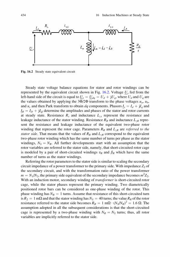
Steady state voltage balance equations for stator and rotor windings can be
represented by the equivalent circuit shown in Fig. 16.2. Voltage Us fed from the
left-hand side of the circuit is equal to Us ¼ Udq ¼ Ud þ jUq, where Ud and Uq are
the values obtained by applying the 3F/2F transform to the phase voltages ua, ub,and uc and then Park transform to obtain dq components. Phasors Is ¼ Id þ jIq andIR ¼ ID þ jIQ determine the amplitudes and phases of the stator and rotor currents
at steady state. Resistance Rs and inductance Lgs represent the resistance and
leakage inductance of the stator winding. Resistance RR and inductance LgR repre-
sent the resistance and leakage inductance of the equivalent two-phase rotor
winding that represent the rotor cage. Parameters RR and LgR are referred to thestator side. That means that the values of RR and LgR correspond to the equivalent
two-phase rotor winding which has the same number of turns per phase as the stator
windings, NS ¼ NR. All further developments start with an assumption that the
rotor variables are referred to the stator side, namely, that short-circuited rotor cage
is modeled by a pair of short-circuited windings aR and bR which have the same
number of turns as the stator windings.
Referring the rotor parameters to the stator side is similar to scaling the secondary
circuit impedance of a power transformer to the primary side. With impedance Z2 ofthe secondary circuit, and with the transformation ratio of the power transformer
m ¼ N1/N2, the primary side equivalent of the secondary impedance becomesm2Z2.With an induction motor, secondary winding of transformer is short-circuited rotorcage, while the stator phases represent the primary winding. Two diametrically
positioned rotor bars can be considered as one-phase winding of the rotor. This
phase winding has NR ¼ 1 turns. Assume that resistance of this short-circuited turn
isR2 ¼ 1mO and that the stator winding hasNS ¼ 40 turns; the value RR of the rotor
resistance referred to the stator side becomes RR ¼ 1 mO ∙ (NS/NR)2 ¼ 1.6 O. The
assumption adopted in all the subsequent considerations is that the short-circuited
cage is represented by a two-phase winding with NR ¼ NS turns; thus, all rotor
variables are implicitly referred to the stator side.
Fig. 16.2 Steady state equivalent circuit
434 16 Induction Machines at Steady State
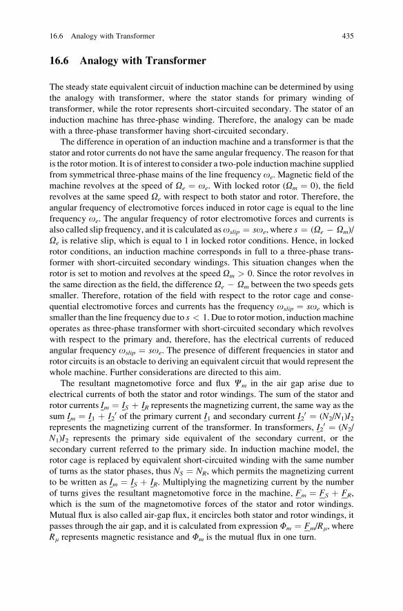
16.6 Analogy with Transformer
The steady state equivalent circuit of induction machine can be determined by using
the analogy with transformer, where the stator stands for primary winding of
transformer, while the rotor represents short-circuited secondary. The stator of an
induction machine has three-phase winding. Therefore, the analogy can be made
with a three-phase transformer having short-circuited secondary.
The difference in operation of an induction machine and a transformer is that the
stator and rotor currents do not have the same angular frequency. The reason for that
is the rotor motion. It is of interest to consider a two-pole inductionmachine supplied
from symmetrical three-phase mains of the line frequency oe. Magnetic field of the
machine revolves at the speed of Oe ¼ oe. With locked rotor (Om ¼ 0), the field
revolves at the same speed Oe with respect to both stator and rotor. Therefore, the
angular frequency of electromotive forces induced in rotor cage is equal to the line
frequency oe. The angular frequency of rotor electromotive forces and currents is
also called slip frequency, and it is calculated asoslip ¼ soe, where s ¼ (Oe � Om)/
Oe is relative slip, which is equal to 1 in locked rotor conditions. Hence, in locked
rotor conditions, an induction machine corresponds in full to a three-phase trans-
former with short-circuited secondary windings. This situation changes when the
rotor is set to motion and revolves at the speed Om > 0. Since the rotor revolves in
the same direction as the field, the difference Oe � Om between the two speeds gets
smaller. Therefore, rotation of the field with respect to the rotor cage and conse-
quential electromotive forces and currents has the frequency oslip ¼ soe which is
smaller than the line frequency due to s < 1. Due to rotor motion, inductionmachine
operates as three-phase transformer with short-circuited secondary which revolves
with respect to the primary and, therefore, has the electrical currents of reduced
angular frequency oslip ¼ soe. The presence of different frequencies in stator and
rotor circuits is an obstacle to deriving an equivalent circuit that would represent the
whole machine. Further considerations are directed to this aim.
The resultant magnetomotive force and flux Cm in the air gap arise due to
electrical currents of both the stator and rotor windings. The sum of the stator and
rotor currents Im ¼ IS þ IR represents the magnetizing current, the same way as the
sum Im ¼ I1 þ I20 of the primary current I1 and secondary current I2
0 ¼ (N2/N1)I2represents the magnetizing current of the transformer. In transformers, I2
0 ¼ (N2/
N1)I2 represents the primary side equivalent of the secondary current, or the
secondary current referred to the primary side. In induction machine model, the
rotor cage is replaced by equivalent short-circuited winding with the same number
of turns as the stator phases, thus NS ¼ NR, which permits the magnetizing current
to be written as Im ¼ IS þ IR. Multiplying the magnetizing current by the number
of turns gives the resultant magnetomotive force in the machine, Fm ¼ FS þ FR,
which is the sum of the magnetomotive forces of the stator and rotor windings.
Mutual flux is also called air-gap flux, it encircles both stator and rotor windings, it
passes through the air gap, and it is calculated from expression Fm ¼ Fm/Rm, where
Rm represents magnetic resistance and Fm is the mutual flux in one turn.
16.6 Analogy with Transformer 435
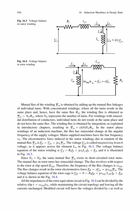
Mutual flux of the windingCm is obtained by adding up the mutual flux linkages
of individual turns. With concentrated windings, where all the turns reside in the
same place and, hence, have the same flux Fm, the winding flux is obtained as
Cm ¼ NNFm, where NN represents the number of turns. For windings with sinusoi-
dal distribution of conductors, individual turns do not reside at the same place and
do not have the same flux. The winding flux is obtained by integration, as explained
in introductory chapters, resulting in Cm ¼ (p/4)NNFm. In the stator phase
windings of an induction machine, the flux has sinusoidal change at the angular
frequency of the supply voltages. Mains supplied machines have the line frequency
oe. The electromotive force induced in the stator windings due to rotation of the
mutual fluxCm is ES ¼ Um ¼ joeCm. The voltageUm is calledmagnetizing branchvoltage, as it appears across the element Lm in Fig. 16.3. The voltage balance
equation of the stator winding is US ¼ RSIS þ joeLgSIS þ ES, and it is illustrated
in Fig. 16.3.
Since NS ¼ NR, the same mutual flux Cm exists in short-circuited rotor turns.
The mutual flux in rotor turns has sinusoidal change. The flux revolves with respect
to the rotor at slip speed Oslip. Therefore, the frequency of the flux changes is oslip.
The flux changes result in the rotor electromotive force ER ¼ sUm ¼ joslipCm. The
voltage balance equation of the rotor cage is UR ¼ 0 ¼ RRIR þ joslip LgR IR þ ER,
and it is shown in the Fig. 16.4.
All the impedances of the rotor equivalent circuit in Fig. 16.4 can be divided by the
relative slip s ¼ oslip/oe, while maintaining the circuit topology and leaving all the
currents unchanged. Modified circuit will have the voltages divided by s as well as
Fig. 16.3 Voltage balance
in stator winding
Fig. 16.4 Voltage balance
in rotor winding
436 16 Induction Machines at Steady State
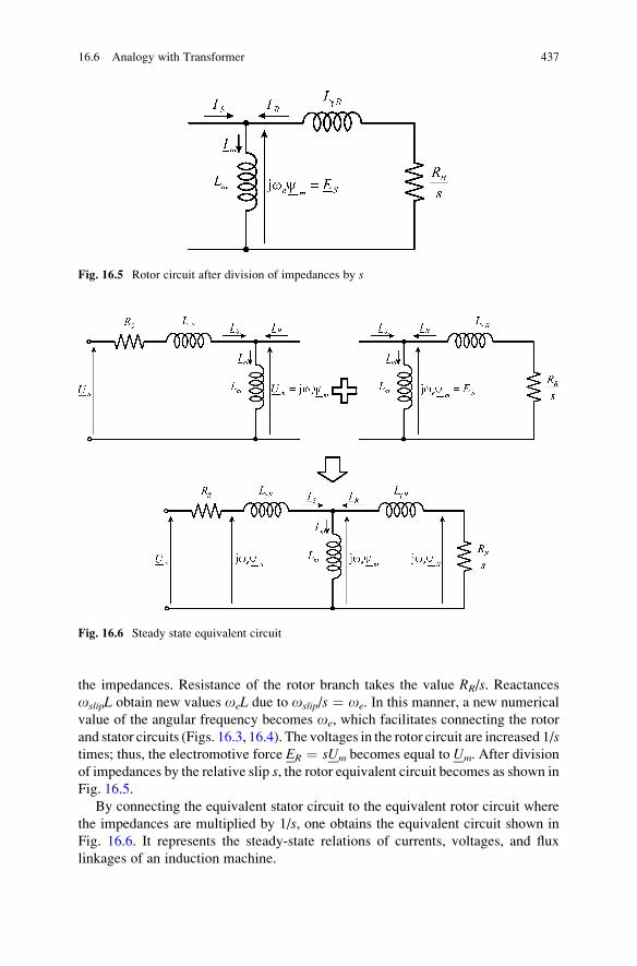
the impedances. Resistance of the rotor branch takes the value RR/s. ReactancesoslipL obtain new values oeL due to oslip/s ¼ oe. In this manner, a new numerical
value of the angular frequency becomes oe, which facilitates connecting the rotor
and stator circuits (Figs. 16.3, 16.4). The voltages in the rotor circuit are increased 1/stimes; thus, the electromotive force ER ¼ sUm becomes equal to Um. After division
of impedances by the relative slip s, the rotor equivalent circuit becomes as shown in
Fig. 16.5.
By connecting the equivalent stator circuit to the equivalent rotor circuit where
the impedances are multiplied by 1/s, one obtains the equivalent circuit shown in
Fig. 16.6. It represents the steady-state relations of currents, voltages, and flux
linkages of an induction machine.
Fig. 16.5 Rotor circuit after division of impedances by s
Fig. 16.6 Steady state equivalent circuit
16.6 Analogy with Transformer 437
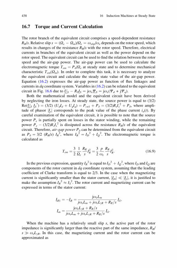
16.7 Torque and Current Calculation
The rotor branch of the equivalent circuit comprises a speed-dependent resistance
RR/s. Relative slip s ¼ (Oe � Om)/Oe ¼ oslip/oe depends on the rotor speed, which
results in changes of the resistance RR/s with the rotor speed. Therefore, electrical
currents in branches of the equivalent circuit as well as the power depend on the
rotor speed. The equivalent circuit can be used to find the relation between the rotor
speed and the air-gap power. The air-gap power can be used to calculate the
electromagnetic torque Tem ¼ Pd/Oe at steady state and to determine mechanical
characteristic Tem(Om). In order to complete this task, it is necessary to analyze
the equivalent circuit and calculate the steady state value of the air-gap power.
Equation (16.2) expresses the air-gap power as function of flux linkages and
currents in dq coordinate system. Variables in (16.2) can be related to the equivalent
circuit in Fig. 16.6 due to US � RSIS ¼ joeCS ¼ joe(Cd + jCq).
Both the mathematical model and the equivalent circuit have been derived
by neglecting the iron losses. At steady state, the source power is equal to (3/2)
Re(US IS*) ¼ (3/2) (UdId þ UqIq) ¼ Pcu1 þ Pd ¼ (3/2)RsIs
2 þ Pd, where ampli-
tude of phasor jIsj corresponds to the peak value of the phase current ia(t). Bycareful examination of the equivalent circuit, it is possible to note that the source
power Pe is partially spent on losses in the stator winding, while the remaining
power Pe � (3/2)RsIs2 is dissipated across the resistance RR/s of the equivalent
circuit. Therefore, air-gap power Pd can be determined from the equivalent circuit
as Pd ¼ 3/2 (RR/s) IR2, where IR
2 ¼ ID2 þ IQ
2. The electromagnetic torque is
calculated as
Tem ¼ 3
2
1
Oe
RR
sI2R ¼ 3
2
p
oe
RR
sI2R: (16.9)
In the previous expression, quantity IR2 is equal to ID
2 þ IQ2, where ID and IQ are
components of the rotor current in dq coordinate system, assuming that the leading
coefficient of Clarke transform is equal to 2/3. In the case when the magnetizing
current is significantly smaller than the stator current, jImj � jIsj, it is justified to
make the assumption IR2 � IS
2. The rotor current and magnetizing current can be
expressed in terms of the stator current:
IR1 ¼ �IR ¼ joeLmjoeLm þ joeLgR þ RR=s
IS;
Im ¼ joeLgR þ RR=s
joeLm þ joeLgR þ RR=sIS:
When the machine has a relatively small slip s, the active part of the rotor
impedance is significantly larger than the reactive part of the same impedance, RR/
s � oeLgR. In this case, the magnetizing current and the rotor current can be
approximated as
438 16 Induction Machines at Steady State
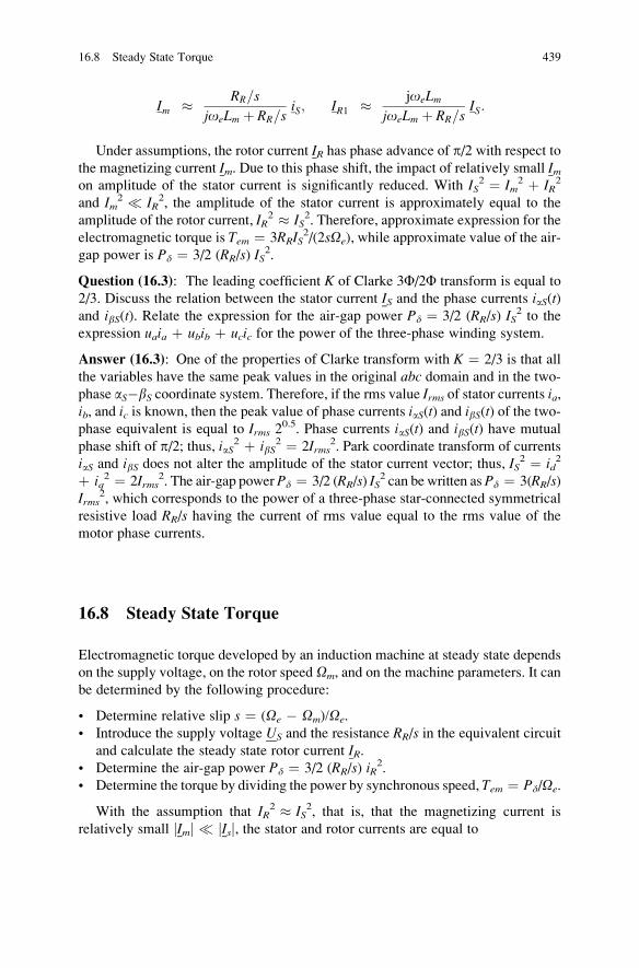
Im � RR=s
joeLm þ RR=siS; IR1 � joeLm
joeLm þ RR=sIS:
Under assumptions, the rotor current IR has phase advance of p/2 with respect tothe magnetizing current Im. Due to this phase shift, the impact of relatively small Imon amplitude of the stator current is significantly reduced. With IS
2 ¼ Im2 þ IR
2
and Im2 � IR
2, the amplitude of the stator current is approximately equal to the
amplitude of the rotor current, IR2 � IS
2. Therefore, approximate expression for the
electromagnetic torque is Tem ¼ 3RRIS2/(2sOe), while approximate value of the air-
gap power is Pd ¼ 3/2 (RR/s) IS2.
Question (16.3): The leading coefficient K of Clarke 3F/2F transform is equal to
2/3. Discuss the relation between the stator current IS and the phase currents iaS(t)and ibS(t). Relate the expression for the air-gap power Pd ¼ 3/2 (RR/s) IS
2 to the
expression uaia þ ubib þ ucic for the power of the three-phase winding system.
Answer (16.3): One of the properties of Clarke transform with K ¼ 2/3 is that all
the variables have the same peak values in the original abc domain and in the two-
phase aS�bS coordinate system. Therefore, if the rms value Irms of stator currents ia,ib, and ic is known, then the peak value of phase currents iaS(t) and ibS(t) of the two-phase equivalent is equal to Irms 2
0.5. Phase currents iaS(t) and ibS(t) have mutual
phase shift of p/2; thus, iaS2 þ ibS
2 ¼ 2Irms2. Park coordinate transform of currents
iaS and ibS does not alter the amplitude of the stator current vector; thus, IS2 ¼ id
2
þ iq2 ¼ 2Irms
2. The air-gap powerPd ¼ 3/2 (RR/s) IS2 can be written as Pd ¼ 3(RR/s)
Irms2, which corresponds to the power of a three-phase star-connected symmetrical
resistive load RR/s having the current of rms value equal to the rms value of the
motor phase currents.
16.8 Steady State Torque
Electromagnetic torque developed by an induction machine at steady state depends
on the supply voltage, on the rotor speed Om, and on the machine parameters. It can
be determined by the following procedure:
• Determine relative slip s ¼ (Oe � Om)/Oe.
• Introduce the supply voltage US and the resistance RR/s in the equivalent circuit
and calculate the steady state rotor current IR.• Determine the air-gap power Pd ¼ 3/2 (RR/s) iR
2.
• Determine the torque by dividing the power by synchronous speed, Tem ¼ Pd/Oe.
With the assumption that IR2 � IS
2, that is, that the magnetizing current is
relatively small jImj � jIsj, the stator and rotor currents are equal to
16.8 Steady State Torque 439
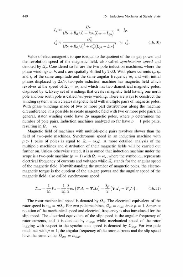
IS �US
RS þ RR=sð Þ þ joe LgR þ LgS� � � IR;
I2S �U2
S
RS þ RR=sð Þ2 þ o2e LgR þ LgS� �2 � I2R: (16.10)
Value of electromagnetic torque is equal to the quotient of the air-gap power and
the revolution speed of the magnetic field, also called synchronous speed and
denoted by Oe. Considered so far are the two-pole induction machines, where the
phase windings a, b, and c are spatially shifted by 2p/3. With phase currents ia, ib,and ic of the same amplitude and the same angular frequency oe and with initial
phases displaced by 2p/3, two-pole induction machine has magnetic field which
revolves at the speed of Oe ¼ oe and which has two diametrical magnetic poles,
displaced by p. Every set of windings that creates magnetic field having one north
pole and one south pole is called two-pole winding. There are ways to construct thewinding system which creates magnetic field with multiple pairs of magnetic poles.
With phase windings made of two or more part distributions along the machine
circumference, it is possible to create magnetic field with two or more pole pairs. In
general, stator winding could have 2p magnetic poles, where p determines the
number of pole pairs. Induction machines analyzed so far have p ¼ 1 pole pairs,
resulting in Oe ¼ oe.
Magnetic field of machines with multiple-pole pairs revolves slower than the
field of two-pole machines. Synchronous speed in an induction machine with
p > 1 pairs of poles is equal to Oe ¼ oe/p. A more detailed analysis of the
multipole machines and distribution of their magnetic fields will be carried out
further on. Unless otherwise stated, it is assumed that induction machine under the
scope is a two-pole machine (p ¼ 1) withOe ¼ oe, where the symboloe represents
electrical frequency of currents and voltages while Oe stands for the angular speed
of the magnetic field. Notwithstanding the number of magnetic poles, the electro-
magnetic torque is the quotient of the air-gap power and the angular speed of the
magnetic field, also called synchronous speed:
Tem ¼ 1
OePd ¼ 1
Oe
3
2oe CdIq �CqId� � ¼ 3p
2CdIq �CqId� �
: (16.11)
The rotor mechanical speed is denoted by Om. The electrical equivalent of the
rotor speed is om ¼ pOm. For two-pole machines, Om ¼ om, since p ¼ 1. Separate
notation of the mechanical speed and electrical frequency is also introduced for the
slip speed. The electrical equivalent of the slip speed is the angular frequency of
rotor currents, and it is denoted by oslip, while mechanical speed of the rotor
lagging with respect to the synchronous speed is denoted by Oslip. For two-pole
machines with p ¼ 1, the angular frequency of the rotor currents and the slip speed
have the same value, Oslip ¼ oslip.
440 16 Induction Machines at Steady State
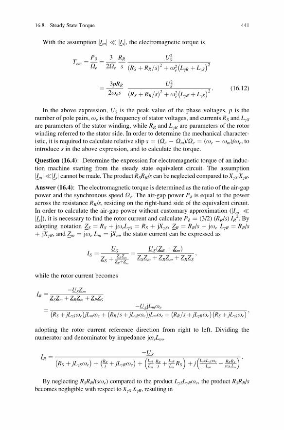
With the assumption jImj � jIsj, the electromagnetic torque is
Tem ¼ Pd
Oe¼ 3
2Oe
RR
s
U2S
RS þ RR=sð Þ2 þ o2e LgR þ LgS� �2
¼ 3pRR
2oes
U2S
RS þ RR=sð Þ2 þ o2e LgR þ LgS� �2 : (16.12)
In the above expression, US is the peak value of the phase voltages, p is the
number of pole pairs, oe is the frequency of stator voltages, and currents RS and LgSare parameters of the stator winding, while RR and LgR are parameters of the rotor
winding referred to the stator side. In order to determine the mechanical character-
istic, it is required to calculate relative slip s ¼ (Oe � Om)/Oe ¼ (oe � om)/oe, to
introduce s in the above expression, and to calculate the torque.
Question (16.4): Determine the expression for electromagnetic torque of an induc-
tion machine starting from the steady state equivalent circuit. The assumption
jImj �jIsj cannot be made. The product RSRR/s can be neglected compared to XgS XgR.
Answer (16.4): The electromagnetic torque is determined as the ratio of the air-gap
power and the synchronous speed Oe. The air-gap power Pd is equal to the power
across the resistance RR/s, residing on the right-hand side of the equivalent circuit.
In order to calculate the air-gap power without customary approximation (jImj �jIsj), it is necessary to find the rotor current and calculate Pd ¼ (3/2) (RR/s) IR
2. By
adopting notation ZS ¼ RS þ joeLgS ¼ RS þ jXgS, ZR ¼ RR/s þ joe LgR ¼ RR/sþ jXgR, and Zm ¼ joe Lm ¼ jXm, the stator current can be expressed as
IS ¼US
ZS þ ZRZm
ZRþZm
¼ US ZR þ Zmð ÞZSZm þ ZRZm þ ZRZS
;
while the rotor current becomes
IR ¼ �USZm
ZSZm þ ZRZm þ ZRZS
¼ �USjLmoe
RS þ jLgSoe
� �jLmoe þ RR=sþ jLgRoe
� �jLmoe þ RR=sþ jLgRoe
� �RS þ jLgSoe
� � ;
adopting the rotor current reference direction from right to left. Dividing the
numerator and denominator by impedance joeLm,
IR ¼ �US
RS þ jLgSoe
� �þ RR
s þ jLgRoe
� �þ LgSLm
RR
s þ LgRLm
RS
� �þ j
LgRLgSoe
Lm� RRRS
soeLm
� � :
By neglecting RSRR/(soe) compared to the product LgSLgRoe, the product RSRR/sbecomes negligible with respect to XgS XgR, resulting in
16.8 Steady State Torque 441
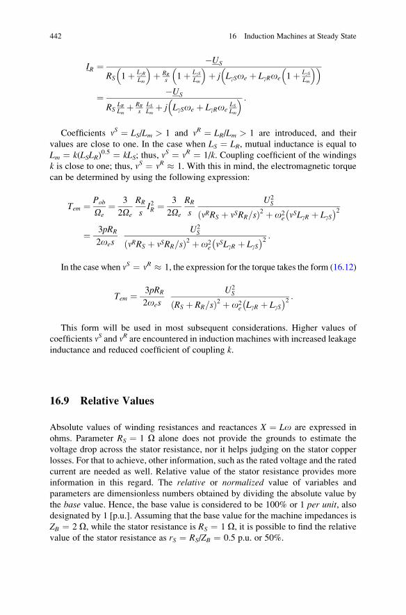
IR ¼ �US
RS 1þ LgRLm
� �þ RR
s 1þ LgSLm
� �þ j LgSoe þ LgRoe 1þ LgS
Lm
� �� �
¼ �US
RSLRLm
þ RR
sLSLm
þ j LgSoe þ LgRoeLSLm
� � :
Coefficients nS ¼ LS/Lm > 1 and nR ¼ LR/Lm > 1 are introduced, and their
values are close to one. In the case when LS ¼ LR, mutual inductance is equal to
Lm ¼ k(LSLR)0.5 ¼ kLS; thus, n
S ¼ nR ¼ 1/k. Coupling coefficient of the windings
k is close to one; thus, nS ¼ nR � 1. With this in mind, the electromagnetic torque
can be determined by using the following expression:
Tem ¼ Pob
Oe¼ 3
2Oe
RR
sI2R ¼ 3
2Oe
RR
s
U2S
nRRS þ nSRR=sð Þ2 þ o2e nSLgR þ LgS� �2
¼ 3pRR
2oes
U2S
nRRS þ nSRR=sð Þ2 þ o2e nSLgR þ LgS� �2 :
In the case when nS ¼ nR � 1, the expression for the torque takes the form (16.12)
Tem ¼ 3pRR
2oes
U2S
RS þ RR=sð Þ2 þ o2e LgR þ LgS� �2 :
This form will be used in most subsequent considerations. Higher values of
coefficients nS and nR are encountered in induction machines with increased leakage
inductance and reduced coefficient of coupling k.
16.9 Relative Values
Absolute values of winding resistances and reactances X ¼ Lo are expressed in
ohms. Parameter RS ¼ 1 O alone does not provide the grounds to estimate the
voltage drop across the stator resistance, nor it helps judging on the stator copper
losses. For that to achieve, other information, such as the rated voltage and the rated
current are needed as well. Relative value of the stator resistance provides more
information in this regard. The relative or normalized value of variables and
parameters are dimensionless numbers obtained by dividing the absolute value by
the base value. Hence, the base value is considered to be 100% or 1 per unit, alsodesignated by 1 [p.u.]. Assuming that the base value for the machine impedances is
ZB ¼ 2 O, while the stator resistance is RS ¼ 1 O, it is possible to find the relative
value of the stator resistance as rS ¼ RS/ZB ¼ 0.5 p.u. or 50%.
442 16 Induction Machines at Steady State
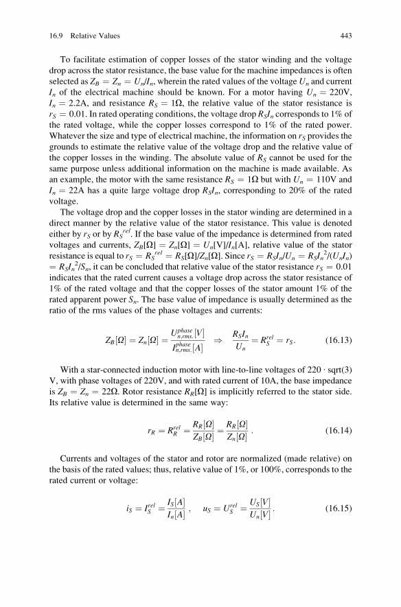
To facilitate estimation of copper losses of the stator winding and the voltage
drop across the stator resistance, the base value for the machine impedances is often
selected as ZB ¼ Zn ¼ Un/In, wherein the rated values of the voltage Un and current
In of the electrical machine should be known. For a motor having Un ¼ 220V,
In ¼ 2.2A, and resistance RS ¼ 1O, the relative value of the stator resistance is
rS ¼ 0.01. In rated operating conditions, the voltage drop RSIn corresponds to 1% of
the rated voltage, while the copper losses correspond to 1% of the rated power.
Whatever the size and type of electrical machine, the information on rS provides thegrounds to estimate the relative value of the voltage drop and the relative value of
the copper losses in the winding. The absolute value of RS cannot be used for the
same purpose unless additional information on the machine is made available. As
an example, the motor with the same resistance RS ¼ 1O but with Un ¼ 110V and
In ¼ 22A has a quite large voltage drop RSIn, corresponding to 20% of the rated
voltage.
The voltage drop and the copper losses in the stator winding are determined in a
direct manner by the relative value of the stator resistance. This value is denoted
either by rS or by RSrel. If the base value of the impedance is determined from rated
voltages and currents, ZB[O] ¼ Zn[O] ¼ Un[V]/In[A], relative value of the stator
resistance is equal to rS ¼ RSrel ¼ RS[O]/Zn[O]. Since rS ¼ RSIn/Un ¼ RSIn
2/(UnIn)¼ RSIn
2/Sn, it can be concluded that relative value of the stator resistance rS ¼ 0.01
indicates that the rated current causes a voltage drop across the stator resistance of
1% of the rated voltage and that the copper losses of the stator amount 1% of the
rated apparent power Sn. The base value of impedance is usually determined as the
ratio of the rms values of the phase voltages and currents:
ZB O½ � ¼ Zn O½ � ¼ Uphasen;rms: V½ �
Iphasen;rms: A½ � ) RSInUn
¼ RrelS ¼ rS: (16.13)
With a star-connected induction motor with line-to-line voltages of 220 ∙ sqrt(3)V, with phase voltages of 220V, and with rated current of 10A, the base impedance
is ZB ¼ Zn ¼ 22O. Rotor resistance RR[O] is implicitly referred to the stator side.
Its relative value is determined in the same way:
rR ¼ RrelR ¼ RR O½ �
ZB O½ � ¼RR O½ �Zn O½ � : (16.14)
Currents and voltages of the stator and rotor are normalized (made relative) on
the basis of the rated values; thus, relative value of 1%, or 100%, corresponds to the
rated current or voltage:
iS ¼ IrelS ¼ IS A½ �In A½ � ; uS ¼ Urel
S ¼ US V½ �Un V½ � : (16.15)
16.9 Relative Values 443
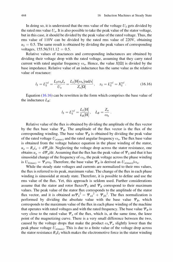
In doing so, it is understood that the rms value of the voltage US gets divided by
the rated rms valueUn. It is also possible to take the peak value of the stator voltage,
but in this case, it should be divided by the peak value of the rated voltage. Thus, the
rms value of 110V can be divided by the rated rms value of 220V, obtaining
uS ¼ 0.5. The same result is obtained by dividing the peak values of corresponding
voltages, 155.56/311.12 ¼ 0.5.
Relative values of reactances and corresponding inductances are obtained by
dividing their voltage drop with the rated voltage, assuming that they carry rated
current with rated angular frequency on. Hence, the value X[O] is divided by the
base impedance. Relative value of an inductance has the same value as the relative
value of reactance:
lS ¼ LrelS ¼ LSonInUn
¼ LS H½ �on rad/s½ �Zn O½ � ; xS ¼ LrelS ¼ Xrel
S : (16.16)
Equation (16.16) can be rewritten in the form which comprises the base value of
the inductance LB:
lS ¼ LrelS ¼ LS H½ �LB H½ � ; LB ¼ Zn
on:
Relative value of the flux is obtained by dividing the amplitude of the flux vector
by the flux base value CB. The amplitude of the flux vector is the flux of the
corresponding winding. The base value CB is obtained by dividing the peak value
of the rated voltage Un(max) and the rated angular frequency on. The flux base value
is obtained from the voltage balance equation in the phase winding of the stator,
ua ¼ Raia þ dCa/dt. Neglecting the voltage drop across the stator resistance, one
obtains ua ¼ dCa/dt. Assuming that the flux has the peak value ofCS and that it has
sinusoidal change of the frequency ofoS, the peak voltage across the phase winding
is US(max) ¼ CSoS. Therefore, the base value CB is derived as Un(max)/on.
While the steady state voltages and currents are normalized to their rms values,
the flux is referred to its peak, maximum value. The change of the flux in each phase
winding is sinusoidal at steady state. Therefore, it is possible to define and use the
rms value of the flux. Yet, this approach is seldom used. Further considerations
assume that the stator and rotor fluxesCS and CR correspond to their maximum
values. The peak value of the stator flux corresponds to the amplitude of the stator
flux vector, and it is obtained asCS2 ¼ CaS
2 þ CbS2. The flux normalization is
performed by dividing the absolute value with the base value CB, which
corresponds to the maximum value of the flux in each phase winding of the machine
that operates with rated voltages and with the rated frequency. The base valueCB is
very close to the rated value Cn of the flux, which is, at the same time, the knee
point of the magnetizing curve. There is a very small difference between the two,
caused by the voltage drops that make the product onCn slightly lower than the
peak phase voltage Un(max). This is due to a finite value of the voltage drop across
the stator resistance RSIS which makes the electromotive force in the stator winding
444 16 Induction Machines at Steady State
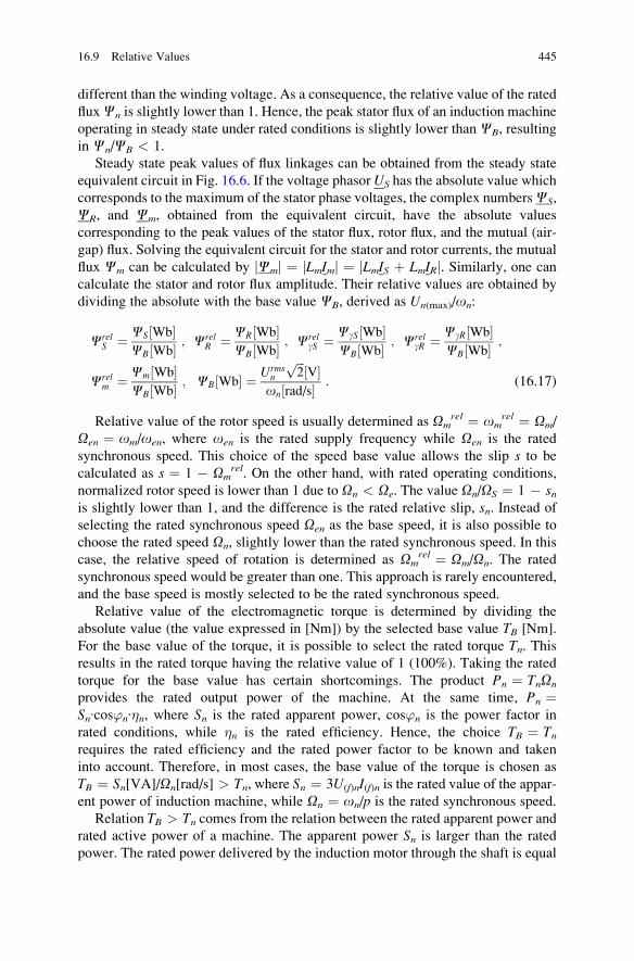
different than the winding voltage. As a consequence, the relative value of the rated
fluxCn is slightly lower than 1. Hence, the peak stator flux of an induction machine
operating in steady state under rated conditions is slightly lower than CB, resulting
in Cn/CB < 1.
Steady state peak values of flux linkages can be obtained from the steady state
equivalent circuit in Fig. 16.6. If the voltage phasorUS has the absolute value which
corresponds to the maximum of the stator phase voltages, the complex numbersCS,
CR, and Cm, obtained from the equivalent circuit, have the absolute values
corresponding to the peak values of the stator flux, rotor flux, and the mutual (air-
gap) flux. Solving the equivalent circuit for the stator and rotor currents, the mutual
flux Cm can be calculated by jCmj ¼ jLmImj ¼ jLmIS þ LmIRj. Similarly, one can
calculate the stator and rotor flux amplitude. Their relative values are obtained by
dividing the absolute with the base value CB, derived as Un(max)/on:
CrelS ¼ CS Wb½ �
CB Wb½ � ; CrelR ¼ CR Wb½ �
CB Wb½ � ; CrelgS ¼ CgS Wb½ �
CB Wb½ � ; CrelgR ¼ CgR Wb½ �
CB Wb½ � ;
Crelm ¼ Cm Wb½ �
CB Wb½ � ; CB Wb½ � ¼ Urmsn
ffiffiffi2
pV½ �
on rad/s½ � : (16.17)
Relative value of the rotor speed is usually determined as Omrel ¼ om
rel ¼ Om/
Oen ¼ om/oen, where oen is the rated supply frequency while Oen is the rated
synchronous speed. This choice of the speed base value allows the slip s to be
calculated as s ¼ 1 � Omrel. On the other hand, with rated operating conditions,
normalized rotor speed is lower than 1 due to On < Oe. The value On/OS ¼ 1 � snis slightly lower than 1, and the difference is the rated relative slip, sn. Instead of
selecting the rated synchronous speed Oen as the base speed, it is also possible to
choose the rated speed On, slightly lower than the rated synchronous speed. In this
case, the relative speed of rotation is determined as Omrel ¼ Om/On. The rated
synchronous speed would be greater than one. This approach is rarely encountered,
and the base speed is mostly selected to be the rated synchronous speed.
Relative value of the electromagnetic torque is determined by dividing the
absolute value (the value expressed in [Nm]) by the selected base value TB [Nm].
For the base value of the torque, it is possible to select the rated torque Tn. Thisresults in the rated torque having the relative value of 1 (100%). Taking the rated
torque for the base value has certain shortcomings. The product Pn ¼ TnOn
provides the rated output power of the machine. At the same time, Pn ¼Sn∙cos’n∙�n, where Sn is the rated apparent power, cos’n is the power factor in
rated conditions, while �n is the rated efficiency. Hence, the choice TB ¼ Tnrequires the rated efficiency and the rated power factor to be known and taken
into account. Therefore, in most cases, the base value of the torque is chosen as
TB ¼ Sn[VA]/On[rad/s] > Tn, where Sn ¼ 3U(f)nI(f)n is the rated value of the appar-ent power of induction machine, while On ¼ on/p is the rated synchronous speed.
Relation TB > Tn comes from the relation between the rated apparent power and
rated active power of a machine. The apparent power Sn is larger than the rated
power. The rated power delivered by the induction motor through the shaft is equal
16.9 Relative Values 445
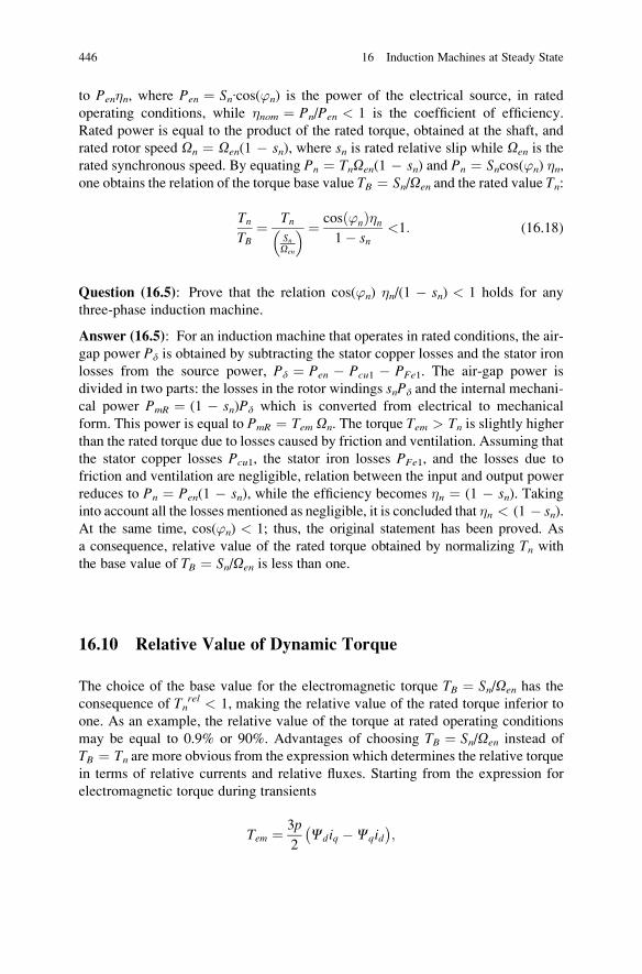
to Pen�n, where Pen ¼ Sn∙cos(’n) is the power of the electrical source, in rated
operating conditions, while �nom ¼ Pn/Pen < 1 is the coefficient of efficiency.
Rated power is equal to the product of the rated torque, obtained at the shaft, and
rated rotor speed On ¼ Oen(1 � sn), where sn is rated relative slip while Oen is the
rated synchronous speed. By equating Pn ¼ TnOen(1 � sn) and Pn ¼ Sncos(’n) �n,one obtains the relation of the torque base value TB ¼ Sn/Oen and the rated value Tn:
TnTB
¼ TnSnOen
� � ¼ cos ’nð Þ�n1� sn
<1: (16.18)
Question (16.5): Prove that the relation cos(’n) �n/(1 � sn) < 1 holds for any
three-phase induction machine.
Answer (16.5): For an induction machine that operates in rated conditions, the air-
gap power Pd is obtained by subtracting the stator copper losses and the stator iron
losses from the source power, Pd ¼ Pen � Pcu1 � PFe1. The air-gap power is
divided in two parts: the losses in the rotor windings snPd and the internal mechani-
cal power PmR ¼ (1 � sn)Pd which is converted from electrical to mechanical
form. This power is equal to PmR ¼ Tem On. The torque Tem > Tn is slightly higherthan the rated torque due to losses caused by friction and ventilation. Assuming that
the stator copper losses Pcu1, the stator iron losses PFe1, and the losses due to
friction and ventilation are negligible, relation between the input and output power
reduces to Pn ¼ Pen(1 � sn), while the efficiency becomes �n ¼ (1 � sn). Takinginto account all the losses mentioned as negligible, it is concluded that �n < (1 � sn).At the same time, cos(’n) < 1; thus, the original statement has been proved. As
a consequence, relative value of the rated torque obtained by normalizing Tn withthe base value of TB ¼ Sn/Oen is less than one.
16.10 Relative Value of Dynamic Torque
The choice of the base value for the electromagnetic torque TB ¼ Sn/Oen has the
consequence of Tnrel < 1, making the relative value of the rated torque inferior to
one. As an example, the relative value of the torque at rated operating conditions
may be equal to 0.9% or 90%. Advantages of choosing TB ¼ Sn/Oen instead of
TB ¼ Tn are more obvious from the expression which determines the relative torque
in terms of relative currents and relative fluxes. Starting from the expression for
electromagnetic torque during transients
Tem ¼ 3p
2Cdiq �Cqid� �
;
446 16 Induction Machines at Steady State
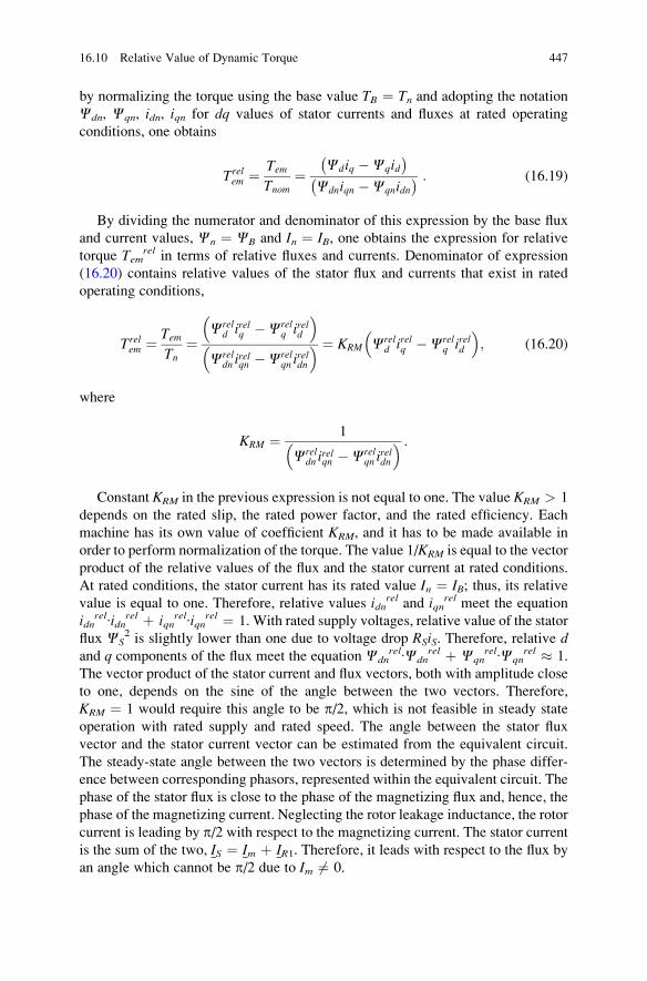
by normalizing the torque using the base value TB ¼ Tn and adopting the notation
Cdn, Cqn, idn, iqn for dq values of stator currents and fluxes at rated operating
conditions, one obtains
Trelem ¼ Tem
Tnom¼ Cdiq �Cqid
� �Cdniqn �Cqnidn� � : (16.19)
By dividing the numerator and denominator of this expression by the base flux
and current values, Cn ¼ CB and In ¼ IB, one obtains the expression for relative
torque Temrel in terms of relative fluxes and currents. Denominator of expression
(16.20) contains relative values of the stator flux and currents that exist in rated
operating conditions,
Trelem ¼ Tem
Tn¼
Creld irelq �Crel
q ireld
� �
Creldn i
relqn �Crel
qn ireldn
� � ¼ KRM Creld irelq �Crel
q ireld
� �; (16.20)
where
KRM ¼ 1
Creldn i
relqn �Crel
qn ireldn
� � :
Constant KRM in the previous expression is not equal to one. The value KRM > 1
depends on the rated slip, the rated power factor, and the rated efficiency. Each
machine has its own value of coefficient KRM, and it has to be made available in
order to perform normalization of the torque. The value 1/KRM is equal to the vector
product of the relative values of the flux and the stator current at rated conditions.
At rated conditions, the stator current has its rated value In ¼ IB; thus, its relativevalue is equal to one. Therefore, relative values idn
rel and iqnrel meet the equation
idnrel∙idnrel þ iqn
rel∙iqnrel ¼ 1. With rated supply voltages, relative value of the stator
flux CS2 is slightly lower than one due to voltage drop RSiS. Therefore, relative d
and q components of the flux meet the equation Cdnrel∙Cdn
rel þ Cqnrel∙Cqn
rel � 1.
The vector product of the stator current and flux vectors, both with amplitude close
to one, depends on the sine of the angle between the two vectors. Therefore,
KRM ¼ 1 would require this angle to be p/2, which is not feasible in steady state
operation with rated supply and rated speed. The angle between the stator flux
vector and the stator current vector can be estimated from the equivalent circuit.
The steady-state angle between the two vectors is determined by the phase differ-
ence between corresponding phasors, represented within the equivalent circuit. The
phase of the stator flux is close to the phase of the magnetizing flux and, hence, the
phase of the magnetizing current. Neglecting the rotor leakage inductance, the rotor
current is leading by p/2 with respect to the magnetizing current. The stator current
is the sum of the two, IS ¼ Im þ IR1. Therefore, it leads with respect to the flux by
an angle which cannot be p/2 due to Im 6¼ 0.
16.10 Relative Value of Dynamic Torque 447
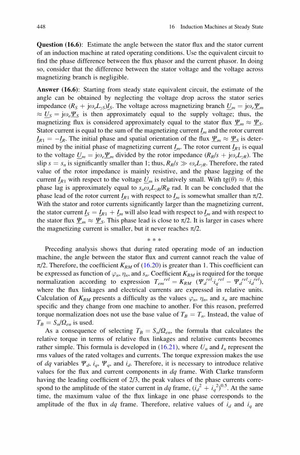
Question (16.6): Estimate the angle between the stator flux and the stator current
of an induction machine at rated operating conditions. Use the equivalent circuit to
find the phase difference between the flux phasor and the current phasor. In doing
so, consider that the difference between the stator voltage and the voltage across
magnetizing branch is negligible.
Answer (16.6): Starting from steady state equivalent circuit, the estimate of the
angle can be obtained by neglecting the voltage drop across the stator series
impedance (RS þ joeLgS)IS. The voltage across magnetizing branch Um ¼ joeCm
� US ¼ joeCS is then approximately equal to the supply voltage; thus, the
magnetizing flux is considered approximately equal to the stator flux Cm � CS.
Stator current is equal to the sum of the magnetizing current Im and the rotor current
IR1 ¼ �IR. The initial phase and spatial orientation of the flux Cm � CS is deter-
mined by the initial phase of magnetizing current Im. The rotor current IR1 is equalto the voltage Um ¼ joeCm divided by the rotor impedance (RR/s þ joeLgR). Theslip s ¼ sn is significantly smaller than 1; thus, RR/s � oeLgR. Therefore, the ratedvalue of the rotor impedance is mainly resistive, and the phase lagging of the
current IR1 with respect to the voltage Um is relatively small. With tg(y) � y, thisphase lag is approximately equal to snoeLgR/RR rad. It can be concluded that the
phase lead of the rotor current IR1 with respect to Im is somewhat smaller than p/2.With the stator and rotor currents significantly larger than the magnetizing current,
the stator current IS ¼ IR1 þ Im will also lead with respect to Im and with respect to
the stator flux Cm � CS. This phase lead is close to p/2. It is larger in cases where
the magnetizing current is smaller, but it never reaches p/2.
* * *
Preceding analysis shows that during rated operating mode of an induction
machine, the angle between the stator flux and current cannot reach the value of
p/2. Therefore, the coefficient KRM of (16.20) is greater than 1. This coefficient can
be expressed as function of ’n, �n, and sn. Coefficient KRM is required for the torque
normalization according to expression Temrel ¼ KRM (Cd
rel∙iqrel � Cdrel∙idrel),
where the flux linkages and electrical currents are expressed in relative units.
Calculation of KRM presents a difficulty as the values ’n, �n, and sn are machine
specific and they change from one machine to another. For this reason, preferred
torque normalization does not use the base value of TB ¼ Tn. Instead, the value ofTB ¼ Sn/Oen is used.
As a consequence of selecting TB ¼ Sn/Oen, the formula that calculates the
relative torque in terms of relative flux linkages and relative currents becomes
rather simple. This formula is developed in (16.21), where Un and In represent therms values of the rated voltages and currents. The torque expression makes the use
of dq variables Cd, iq, Cq, and id. Therefore, it is necessary to introduce relative
values for the flux and current components in dq frame. With Clarke transform
having the leading coefficient of 2/3, the peak values of the phase currents corre-
spond to the amplitude of the stator current in dq frame, (id2 þ iq
2)0.5. At the same
time, the maximum value of the flux linkage in one phase corresponds to the
amplitude of the flux in dq frame. Therefore, relative values of id and iq are
448 16 Induction Machines at Steady State
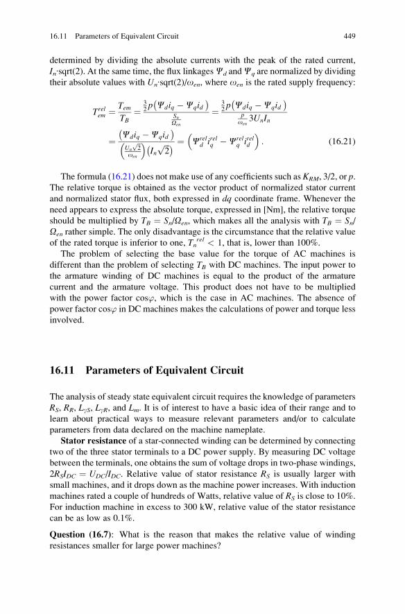
determined by dividing the absolute currents with the peak of the rated current,
In∙sqrt(2). At the same time, the flux linkagesCd andCq are normalized by dividing
their absolute values with Un∙sqrt(2)/oen, where oen is the rated supply frequency:
Trelem ¼ Tem
TB¼
32p Cdiq �Cqid� �
SnOen
¼32p Cdiq �Cqid� �
poen
3UnIn
¼ Cdiq �Cqid� �
Un
ffiffi2
poen
� �Inffiffiffi2
p� � ¼ Creld irelq �Crel
q ireld
� �: (16.21)
The formula (16.21) does not make use of any coefficients such as KRM, 3/2, or p.The relative torque is obtained as the vector product of normalized stator current
and normalized stator flux, both expressed in dq coordinate frame. Whenever the
need appears to express the absolute torque, expressed in [Nm], the relative torque
should be multiplied by TB ¼ Sn/Oen, which makes all the analysis with TB ¼ Sn/Oen rather simple. The only disadvantage is the circumstance that the relative value
of the rated torque is inferior to one, Tnrel < 1, that is, lower than 100%.
The problem of selecting the base value for the torque of AC machines is
different than the problem of selecting TB with DC machines. The input power to
the armature winding of DC machines is equal to the product of the armature
current and the armature voltage. This product does not have to be multiplied
with the power factor cos’, which is the case in AC machines. The absence of
power factor cos’ in DC machines makes the calculations of power and torque less
involved.
16.11 Parameters of Equivalent Circuit
The analysis of steady state equivalent circuit requires the knowledge of parameters
RS, RR, LgS, LgR, and Lm. It is of interest to have a basic idea of their range and to
learn about practical ways to measure relevant parameters and/or to calculate
parameters from data declared on the machine nameplate.
Stator resistance of a star-connected winding can be determined by connecting
two of the three stator terminals to a DC power supply. By measuring DC voltage
between the terminals, one obtains the sum of voltage drops in two-phase windings,
2RSIDC ¼ UDC/IDC. Relative value of stator resistance RS is usually larger with
small machines, and it drops down as the machine power increases. With induction
machines rated a couple of hundreds of Watts, relative value of RS is close to 10%.
For induction machine in excess to 300 kW, relative value of the stator resistance
can be as low as 0.1%.
Question (16.7): What is the reason that makes the relative value of winding
resistances smaller for large power machines?
16.11 Parameters of Equivalent Circuit 449
Answer (16.7): In electrical machines, there are losses in magnetic circuits and in
current circuits, also called iron losses and copper losses. Specific power of iron
losses is the iron loss per unit volume or unit mass of the magnetic circuit. It
depends on magnetic induction Bm and frequency of the field changes in considered
magnetic circuit. Considering two electrical machines with the same flux density
(induction B) and the same frequency, then the specific power of iron losses has the
same values in both machines. Therefore, the ratio of PFe1 and PFe2 is determined
by the ratio of volumes of respective magnetic circuits V1f/V2f, or by the ratio of
their masses m1f/m2f.
Specific power of losses in copper is the amount of loss power per unit volume or
unit mass, and it is dependent on current density [A/mm2] and specific conductivity
s of the metal (copper) used to make the conductors. Considering two electrical
machines with the same current density and with conductors made of the same
material (copper), their specific power of copper losses is equal. The ratio of PCu1
and PCu2 is dependent on the quantity of the material used to make the windings,
namely, the ratio PCu1/PCu2 is determined by the ratio of volumes V1Cu/V2Cu or mass
m1Cu/m2Cu of the copper used in making respective windings.
If one of the two machines has diameter which is two times larger and it has
twice the length of the other, smaller machine, its volume is eight times larger
(V ~ l3) than the volume of the smaller machine. At the same time, assumption is
made that the two machines are similar and that both magnetic circuit and the
windings of the larger machine are obtained by starting from relevant parts of the
smaller machine and doubling their linear dimensions. Assuming that both
machines have the same current density, the same induction Bm, and the same
operating frequency f, then the power of losses of the larger machine is eight times
higher.
Losses of energy in the magnetic and current circuits of electrical machines
generate heat which increases temperatures of the vital parts of the machine.
Maintaining integrity and functionality of machine parts such as the electrical insula-
tion of the windings, ferromagnetic materials, bearings, and other parts requires
containing the machine temperature within safe limits. Excessive temperatures can
cause permanent damage to vital parts of the machine. Therefore, it is necessary to
provide cooling that removes excess heat and keeps the machine temperature within
safe limits. At steady state, when the machine temperature sets to a constant value, the
heat created by the conversion losses within the machine is equal to the heat removed
by cooling. Different cooling methods such as convection, conduction, and radiation
remove the amount of heat which depends on the temperature difference between the
machine and the surrounding environment. The heat transfer is also proportional to the
surface area of the machine parts getting in touch with the environment and also the
contact area with the cooling fluids. The surface is proportional to S ~ l2. Therefore,the larger machine with doubled diameter and twice the axial length can be cooled
with four times larger surface area than the smaller machine.
It can be concluded that machines with l times larger linear dimensions have l3
times higher losses, while their ability to remove heat is increased l2 times. Under
circumstances, the temperature of the machine with l times larger linear dimensions
450 16 Induction Machines at Steady State
is going to increase l times. This statement relies on the assumption that the specific
power of losses remains unaltered. The above consideration shows that larger
machines require more efficient cooling methods and reduction of specific power
of losses. For this reason, large machines are usually designed and made to have
smaller values of magnetic induction Bm and smaller current densities in their
windings. As a consequence, the windings are built of conductors with larger
cross section, which results in smaller winding resistances. Therefore, relative
value of the stator resistance is smaller for machines of larger power. It is necessary
to note that the value RSrel ¼ 0.001, corresponding to machine of 1 MW, actually
means that the copper losses in the stator winding have the power of 1 kW. Namely,
the energy of 1,000 J is converted into heat in each second. Heat removal at rates of
1,000 J per second may require forced cooling. Any further increase in RS would
bring additional copper losses and result in an increase in the winding temperature
that may damage electrical insulation.
Ratio of the power of losses and cooling surface of smaller machines is much
more favorable. Therefore, the problem of cooling is less emphasized, and there is
no need to use more copper by increasing the cross section of conductors. For very
small machines, relative values of RS in excess of 10% can be tolerated. This means
that 10% of the rated power accounts for the copper losses, which introduces the
question of energy efficiency. It is of interest to notice that many small electrical
machines operate intermittently, such as the motors in hand dryers, and remain
disconnected for most of the time. In such cases, the energy that has to be used to
manufacture electrolytic copper required for the motor windings may be more
significant than the energy lost in the copper losses during the machine lifetime.
* * *
Magnetizing inductance Lm determines the magnetizing current Im ¼ IS þ IRwhich is required to achieve desired flux Cm ¼ LmIm. With most induction
machines, magnetizing current Im is much smaller than the rated current. By
analogy with power transformer, considering the stator as the primary winding
and the rotor as the secondary winding, magnetizing current corresponds to no loadcurrent of the transformer, the current that circulates in primary winding when the
secondary winding does not have any current. In the case when an induction
machine is not coupled to mechanical load, the rotor revolves with no external
resistance. The load torque TL is equal to zero. Internal mechanical losses such as
the bearing friction and the air resistance are negligible in most cases. Therefore,
the rotor revolves at the speed which is very close to the synchronous speed and the
relative slip is s � 0. Impedance RR/s takes a very high value; thus, rotor current
can be neglected, and the rotor circuit can be considered open. The equivalent
circuit of the induction machine reduces to a series connection of the stator
resistance RS, the stator leakage inductance LgS, and the magnetizing inductance Lm.The experiment with an induction machine connected to the mains having the
rated voltage and the rated frequency applies the rated supply to the stator windings.
With shaft disconnected from any mechanical load or work machine, the rotor
revolves at synchronous speed. Such experiment is called no load test. At steady
16.11 Parameters of Equivalent Circuit 451
state, the stator current is equal to I0 ¼ USn/(RS þ joenLS). Neglecting the stator
resistance and the leakage inductance, one obtains LS � Lm � USn/(I0 oen).
No load current of induction machines of small power is within range of 50–70%
of the rated current. For high-power machines, no load current can be lower than
20% of the rated current.
Question (16.8): What is the reason that makes the relative no load current smaller
for high-power machines?
Answer (16.8): High-power machines are designed to have smaller value of
magnetic induction Bm in their magnetic circuits. Cooling of high-power
machines is more difficult. Therefore, they are designed to have smaller values
of magnetic induction in iron parts and smaller current density in copper
conductors. The slope DB/DH of the magnetizing characteristic of the ferromag-
netic material (B–H curve) is higher in regions that are closer to the origin of the
B–H plane. Consequently, magnetic permeability is higher, which reduces
magnetic resistance RmFe of the iron parts of the magnetic circuit. Moreover,
high-power machines have larger dimensions and more favorable ratio of the air
gap d and machine diameter D. Due to smaller d/D ratio, the air-gap part of
magnetic resistance is smaller. Smaller values of magnetic resistance result in
higher values of inductance, which is inversely proportional to magnetic resis-
tance due to L ¼ N2/Rm. Self-inductance of the stator winding LS is proportional tothe ratio N2/Rm, while magnetizing inductance is slightly smaller due to Lm ¼ kLS,where coupling coefficient k is somewhat lower than one. It can be concluded that
a lower magnetic resistance and improved d/D ratio of high-power machines
result in higher relative values of their magnetizing inductance Lm and smaller
relative values of their no load currents.
* * *
Leakage inductances of the stator and rotor are coefficients of proportionality
between the respective leakage flux and winding current. With NS ¼ NR and LS ¼LR, LgS ¼ (1 � k)LS, LgR ¼ (1 � k)LS, and Lm ¼ kLS. The number of rotor turns
NR is related to virtual, equivalent rotor winding which replaces the rotor cage.
Therefore, in most cases, the stator and rotor leakage inductances can be considered
equal,2 LgS � LgR. In cases where short-circuited rotor cage is represented by
equivalent rotor winding having the same number of turns as the stator, NS ¼ NR,
all the rotor parameters are referred to the stator side without scaling due to the
transfer ratio m ¼ NS/NR ¼ 1. Inductances of the stator and rotor are proportional
to squared number of turns and inversely proportional to magnetic resistance. The
mutual and leakage fluxes of the stator and rotor windings exist in magnetic circuits
2 There is no unique way to determine the mutual flux (i.e., the air-gap flux). The surface used to
calculate the surface integral of the magnetic induction and find the air-gap flux passes through air
gap, but it can be placed closer to the stator or closer to the rotor. Therefore, the same machine can
be modeled by using different sets of values (LgS, LgR, Lm). It is of interest to note that all of these
sets provide correct mathematical model of the machine behavior.
452 16 Induction Machines at Steady State
with approximately equal lengths and cross sections. They share the same air gap,
and they are made of the same iron sheets. For this reason, it is justified to assume
that LS � LR and LgS � LgR. The assumption is valid for majority of induction
machines. Exceptions to this appear with induction machines with large differences
in dimensions and shapes of the stator and rotor slots.
An approximate value of leakage inductances can be determined by the short-circuit test. During this test, the rotor of the induction machine is locked. It cannotmove and its speed is equal to zero. During the test, the rotor motion is prevented by
mechanical means. In locked rotor conditions, the relative slip is equal to one,
s ¼ 1. Impedance RR/s obtains relatively small value RR. By neglecting the
magnetizing current, the equivalent impedance of the motor becomes US/IS ¼ RS
þ RR þ joeLgS þ joeLgR. For machines with rated power in excess to 10 kW,
relative values of resistances RS and RR are very low, and they can be neglected.
The leakage inductance is then determined as LgS � LgR ¼ ½ US/(ISoe), where US
and IS are the rms values of the stator voltages and currents measured during the
short-circuit test. With small machines, the winding resistance cannot be neglected.
During the short-circuit test, it is necessary to determine the phase shift between the
voltages and currents in order to distinguish between the real and imaginary parts of
the short-circuit impedance ZK ¼ RS þ RR þ joeLgS þ joeLgR.The short-circuit reactance oen(LgR þ LgS) at rated conditions has the relative
value that ranges from 0.05 up to 0.3. Smaller values are met in lower power low-
voltage (400 V) machines, while higher values correspond to induction machines
for medium voltages (6 kV) and powers of the order of 1 MW. In high-power and
high-voltage machines, distances between conductors of stator and rotor windings
are larger. Larger distances are necessary for the purposes of a more efficient
cooling. At the same time, insulation between conductors has to withstand higher
voltages, which contributes to an increased distance between conductors. As a
consequence, the coupling coefficient k between stator and rotor windings is
smaller, which increases leakage inductances due to LgS � LgR � (1 � k)LS:
LgS ¼ LS � Lm; LgR ¼ LR � Lm: (16.22)
The short-circuit reactance of an induction machine is approximately equal to
the sum of the stator and rotor leakage reactances oen(LgR þ LgS) ¼ XgS þ XgR.
A small difference between the actual short-circuit reactance Lgeoen and the sum of
the stator and rotor leakage reactances exists due to a finite value of Lmoen.
The actual value of the short-circuit reactance can be determined by considering
equivalent transformer. The stator and rotor windings of an induction machine are
coupled by magnetic field in the same way as the primary and secondary windings
of a transformer. A short-circuited induction motor with RS, RR � oen(LgR þ LgS)is equivalent to a transformer with short-circuited secondary and with negligible
winding resistances. The input (equivalent) inductance Lge ¼ Xge/oen of a short-
circuited induction machine, also called the equivalent leakage inductance, can be
calculated from the circuit in Fig. 16.7:
16.11 Parameters of Equivalent Circuit 453
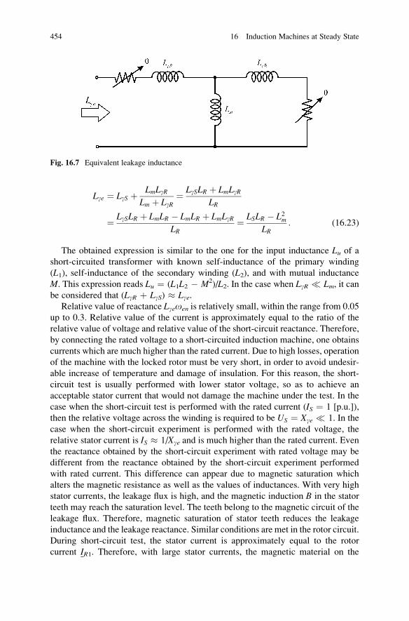
Lge ¼ LgS þ LmLgRLm þ LgR
¼ LgSLR þ LmLgRLR
¼ LgSLR þ LmLR � LmLR þ LmLgRLR
¼ LSLR � L2mLR
: (16.23)
The obtained expression is similar to the one for the input inductance Lu of ashort-circuited transformer with known self-inductance of the primary winding
(L1), self-inductance of the secondary winding (L2), and with mutual inductance
M. This expression reads Lu ¼ (L1L2 � M2)/L2. In the case when LgR � Lm, it canbe considered that (LgR þ LgS) � Lge.
Relative value of reactance Lgeoen is relatively small, within the range from 0.05
up to 0.3. Relative value of the current is approximately equal to the ratio of the
relative value of voltage and relative value of the short-circuit reactance. Therefore,
by connecting the rated voltage to a short-circuited induction machine, one obtains
currents which are much higher than the rated current. Due to high losses, operation
of the machine with the locked rotor must be very short, in order to avoid undesir-
able increase of temperature and damage of insulation. For this reason, the short-
circuit test is usually performed with lower stator voltage, so as to achieve an
acceptable stator current that would not damage the machine under the test. In the
case when the short-circuit test is performed with the rated current (IS ¼ 1 [p.u.]),
then the relative voltage across the winding is required to be US ¼ Xge � 1. In the
case when the short-circuit experiment is performed with the rated voltage, the
relative stator current is IS � 1/Xge and is much higher than the rated current. Even
the reactance obtained by the short-circuit experiment with rated voltage may be
different from the reactance obtained by the short-circuit experiment performed
with rated current. This difference can appear due to magnetic saturation which
alters the magnetic resistance as well as the values of inductances. With very high
stator currents, the leakage flux is high, and the magnetic induction B in the stator
teeth may reach the saturation level. The teeth belong to the magnetic circuit of the
leakage flux. Therefore, magnetic saturation of stator teeth reduces the leakage
inductance and the leakage reactance. Similar conditions are met in the rotor circuit.
During short-circuit test, the stator current is approximately equal to the rotor
current IR1. Therefore, with large stator currents, the magnetic material on the
Fig. 16.7 Equivalent leakage inductance
454 16 Induction Machines at Steady State
path of the rotor leakage flux reaches saturation, which leads to an increase of
magnetic resistance and a decrease of the rotor leakage inductance. The short-
circuit test with elevated currents demonstrates that the induction machine is a
nonlinear system. Mathematical model and the equivalent circuit developed since
describe the machine behavior provided that the modeling approximations are valid
and that the machine operates with all the variables remaining reasonably close to
rated conditions. In cases with very large currents, very large speeds, excessive slip
frequencies, or excessive flux amplitudes, parameters of the steady state equivalent
circuit cannot be considered constant. Moreover, even the steady state equivalent
circuit may not be the adequate way to describe the machine behavior. Nonlinear
phenomena in induction machines are intentionally kept out of this book.
Resistance of the rotor winding referred to the stator side is denoted by RR.
Relative value of parameter RR is usually close to the relative value of RS. In low-
power machines, relative RR is close to 10%, while for induction machines in excess
to 1 MW, it could be as low as RR � 0.1%. In essence, the actual resistance of the
rotor bars can hardly be measured. Yet, parameter RR in the equivalent circuit could
be determined from the equivalent circuit. With known US and IS, and with all the
parameters of the equivalent circuit known, except for RR/s, it is possible to
calculate the value of RR/s expressed in [O]. Provided that the rotor speed is
available as well, one can calculate the relative slip and obtain precise value of
the rotor resistance. The following considerations provide the means for finding a
quick estimate of the rotor resistance.
16.11.1 Rotor Resistance Estimation
The rotor resistance RR can be calculated from the impedance obtained by the
locked rotor test. This impedance is ZK � RS þ RR þ joeLgS þ joeLgR. Taking thereal part of the locked rotor test and subtracting the stator resistance, it is possible to
obtain the parameter RR which makes part of the short-circuit impedance. This
value may be different than the resistance encountered by the rotor currents having
the rated slip frequency. In the locked rotor test, the rotor currents have the
line frequency, the same as the stator currents. At rated operating conditions, the
frequency of rotor currents ranges from fslip ~ 0.5 to fslip ~ 5 Hz. Due to relatively
large cross section of rotor conductors, the skin effect is emphasized even at the line
frequency. The skin effect in rotor bars consists in pushing the rotor currents toward
the air gap and reducing the currents deep in the rotor slots. This uneven distribution
of currents leads to an increase in the rotor equivalent resistance at elevated
frequencies. Therefore, the rotor resistance at fslip ¼ 50 Hz, measured in the
short-circuit test, is considerably higher than the rotor resistance at rated slip
frequency.
Another way of estimating the parameter RR is based on determining the time
constant of the rotor circuit, tR ¼ LR/RR. The rotor time constant tR can be
16.11 Parameters of Equivalent Circuit 455
determined from the voltage change between the two terminals of the stator
winding. This voltage change has to be measured after disconnecting the machine
from the mains. In this case, the voltage between the stator terminals reflects the
changes of the induced electromotive force, proportional to the rotor flux. In the
prescribed conditions, the flux decays with the time constant tR, which provides thegrounds for RR estimation. Before commencing with measurement, induction
machine should be running with no load (TL ¼ 0), connected to the mains which
provides the rated voltage of the rated frequency. It is assumed that the machine
accelerated up to the synchronous speed, that the steady state has been established,
and that the torque, power, and slip are close to zero, while the magnetic circuits has
the rated flux. At this point, a safe, isolated voltage probe3 should be connected
between the two terminals of the stator windings, bringing the line voltage to a
digital storage oscilloscope. Upon disconnecting the machine from the mains, the
stator currents drop to zero. Considering the equivalent circuit, the stator contour
remains open, while the remaining rotor current circulates through the magnetizing
branch. Hence, the residual rotor current provides the magnetizing current and
supports the flux. The short-circuited rotor cage opposes to any change of the flux,
attempting to preserve the flux found at the instant of disconnecting the mains. The
rotor counter electromotive forces and currents are induced to oppose to the flux
change. It is of interest to study the change of the rotor current at the instant of
disconnecting the mains. Considering the equivalent circuit prior to disconnection,
the rotor current was close to zero, while the stator current was equal to the
magnetizing current Im. Disconnecting the stator winding from the mains cuts the
stator current down to zero,4 while the magnetizing current shifts into the rotor
circuit. The rotor circuit is established due to short-circuited cage attempting to
maintain the flux unaltered. Hence, although the machine is disconnected from the
mains, the magnetizing flux is maintained by the rotor cage. Therefore, residual flux
revolves within the machine at the rotor speed, which remains close to the synchro-
nous speed. At first, there are no significant changes of the flux amplitude.
Electromotive force Cmoe is induced in the stator windings. It has the amplitude
close to the rated voltage, the frequency close to the supply frequency, and it can be
measured between the open stator terminals. It is assumed that, in the absence of
mechanical load, the rotor speed remains constant throughout the experiment.
3 The instant of opening the switch which connects the stator winding to the mains may result in
transient overvoltages across the contacts being opened and across the voltage probe. Therefore, it
is advisable to use the probe that withstands the voltages in excess to the rated voltages. With
0.4 kV machines, a 10 kV probe would do. The probe has to be passed through the insulator which
secures galvanic insulation between the motor terminals and the oscilloscope, where the later has
to be connected to protective ground for safety.4 It may take up to a couple of milliseconds to open the switch contacts and extinguish the electric
arc between the opened contacts, which eventually brings the stator current to zero. The arcing
cannot be avoided, and it is more emphasized when the leakage inductance is larger. As a matter of
fact, the arcing burns the energy of the leakage flux,Wge ~ LgeiS2. The switch opening time is very
short compared to the machine dynamics, and it is neglected in the present discussion.
456 16 Induction Machines at Steady State
By time, the amplitude of this electromotive force gradually decays. Since the stator
circuit is open, the rotor current and, hence, the magnetizing current exist in the
contour comprising three elements: Lm, LgR, and RR. Therefore, the current decays
exponentially with the time constant determined by the ratio of inductance and
resistance of the circuit, tR ¼ LR/RR. As a consequence, the envelope of the induced
electromotive force drops according to the law exp(-t/tR). Therefore, by determining
the envelope of the line voltage, the rotor time constant can be estimated as the time
required for the amplitude to drop e times, that is, to reduce to some 37% of the
initial value.
There is also possibility to calculate an approximate value of RR from data
available on the nameplate of the machine. Parameter RR can be estimated from
the equivalent circuit by using the rated voltages and currents. It is necessary to
make a series of assumptions regarding the equivalent circuit in rated conditions.
By neglecting the stator resistance and magnetizing inductance, the equivalent
circuit reduces to series connection of the equivalent reactance Lgeoen and
rotor resistance RR/s. In rated operating conditions, the voltage across the resistanceRR/s of the equivalent circuit is equal to (Un
2 � (InLgeoen)2)1/2. If relative values
are used, thenUn ¼ 1 and In ¼ 1. Reactance Lgeoen has relative value ranging from
0.05 to 0.25. The phasor of the voltage drop across this reactance is orthogonal to
the phasor InRR/s; thus, the voltage drop InLgeoen has no significant impact on the
voltage across the resistance RR/s. With Lgeosn ¼ 0.25 and Un ¼ 1, the relative
value of the rotor voltage InRR/s is 97%. Therefore, it is justifiable to assume that the
rotor voltage in rated conditions is close to 1 relative unit. With rated current in both
stator and rotor windings, impedance RR/sn is equal to Un/In ¼ ZB. On the basis of
introduced approximations, it follows that RR � snZB. In other words, relative valueof rotor resistance rR ¼ RR/ZB is close to the rated value of relative slip sn. Hence,from nameplate of an induction motor that comprise data In ¼ 22 A, Ufn ¼ 220 V
(Uln ¼ 380 V), fn ¼ 50 Hz, and nn ¼ 2,700 rpm, an estimate of the motor parame-
ter RR is snZB ¼ 1 O.
16.12 Analysis of Mechanical Characteristic
The electromagnetic torque of an induction machine is equal to the ratio of the air-
gap power Pd, which is transferred from the stator to the rotor, and synchronous
speed Oe ¼ oe/p, which is the revolving speed of the magnetic field. From the
analysis of the steady state equivalent circuit, the torque can be calculated from
expression
Tem ¼ Pd
Oe¼ 3
2Oe
RR
sI2R :
By solving the equivalent circuit, shown in Fig. 16.8, one can obtain the stator
and rotor currents. Rotor current is equal to
16.12 Analysis of Mechanical Characteristic 457
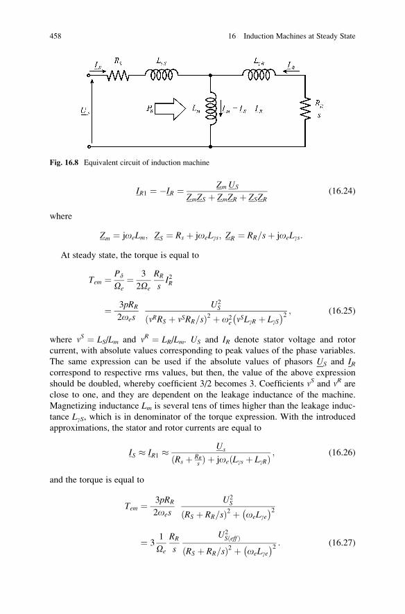
IR1 ¼ �IR ¼ Zm US
ZmZS þ ZmZR þ ZSZR(16.24)
where
Zm ¼ joeLm; ZS ¼ Rs þ joeLgs; ZR ¼ RR=sþ joeLgs:
At steady state, the torque is equal to
Tem ¼ Pd
Oe¼ 3
2Oe
RR
sI2R
¼ 3pRR
2oes
U2S
nRRS þ nSRR=sð Þ2 þ o2e nSLgR þ LgS� �2 ; (16.25)
where nS ¼ LS/Lm and nR ¼ LR/Lm. US and IR denote stator voltage and rotor
current, with absolute values corresponding to peak values of the phase variables.
The same expression can be used if the absolute values of phasors US and IRcorrespond to respective rms values, but then, the value of the above expression
should be doubled, whereby coefficient 3/2 becomes 3. Coefficients nS and nR are
close to one, and they are dependent on the leakage inductance of the machine.
Magnetizing inductance Lm is several tens of times higher than the leakage induc-
tance LgS, which is in denominator of the torque expression. With the introduced
approximations, the stator and rotor currents are equal to
IS � IR1 �Us
ðRs þ RR
s Þ þ joeðLgs þ LgRÞ; (16.26)
and the torque is equal to
Tem ¼ 3pRR
2oes
U2S
RS þ RR=sð Þ2 þ oeLge� �2
¼ 31
Oe
RR
s
U2Sðeff Þ
RS þ RR=sð Þ2 þ oeLge� �2 : (16.27)
Fig. 16.8 Equivalent circuit of induction machine
458 16 Induction Machines at Steady State
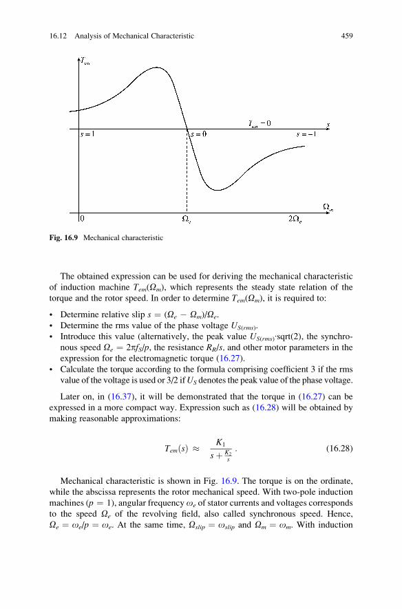
The obtained expression can be used for deriving the mechanical characteristic
of induction machine Tem(Om), which represents the steady state relation of the
torque and the rotor speed. In order to determine Tem(Om), it is required to:
• Determine relative slip s ¼ (Oe � Om)/Oe.
• Determine the rms value of the phase voltage US(rms).
• Introduce this value (alternatively, the peak value US(rms)∙sqrt(2), the synchro-
nous speed Oe ¼ 2pfS/p, the resistance RR/s, and other motor parameters in the
expression for the electromagnetic torque (16.27).
• Calculate the torque according to the formula comprising coefficient 3 if the rms
value of the voltage is used or 3/2 ifUS denotes the peak value of the phase voltage.
Later on, in (16.37), it will be demonstrated that the torque in (16.27) can be
expressed in a more compact way. Expression such as (16.28) will be obtained by
making reasonable approximations:
TemðsÞ � K1
sþ K2
s
: (16.28)
Mechanical characteristic is shown in Fig. 16.9. The torque is on the ordinate,
while the abscissa represents the rotor mechanical speed. With two-pole induction
machines (p ¼ 1), angular frequencyoe of stator currents and voltages corresponds
to the speed Oe of the revolving field, also called synchronous speed. Hence,
Oe ¼ oe/p ¼ oe. At the same time, Oslip ¼ oslip and Om ¼ om. With induction
Fig. 16.9 Mechanical characteristic
16.12 Analysis of Mechanical Characteristic 459
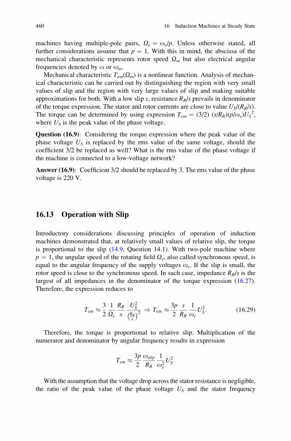
machines having multiple-pole pairs, Oe ¼ oe/p. Unless otherwise stated, all
further considerations assume that p ¼ 1. With this in mind, the abscissa of the
mechanical characteristic represents rotor speed Om but also electrical angular
frequencies denoted by o or om.
Mechanical characteristic Tem(Om) is a nonlinear function. Analysis of mechan-
ical characteristic can be carried out by distinguishing the region with very small
values of slip and the region with very large values of slip and making suitable
approximations for both. With a low slip s, resistance RR/s prevails in denominator
of the torque expression. The stator and rotor currents are close to value US/(RR/s).The torque can be determined by using expression Tem ¼ (3/2) (s/RR)(p/oe)US
2,
where US is the peak value of the phase voltage.
Question (16.9): Considering the torque expression where the peak value of the
phase voltage US is replaced by the rms value of the same voltage, should the
coefficient 3/2 be replaced as well? What is the rms value of the phase voltage if
the machine is connected to a low-voltage network?
Answer (16.9): Coefficient 3/2 should be replaced by 3. The rms value of the phase
voltage is 220 V.
16.13 Operation with Slip
Introductory considerations discussing principles of operation of induction
machines demonstrated that, at relatively small values of relative slip, the torque
is proportional to the slip (14.9, Question 14.1). With two-pole machine where
p ¼ 1, the angular speed of the rotating field Oe, also called synchronous speed, is
equal to the angular frequency of the supply voltages oe. If the slip is small, the
rotor speed is close to the synchronous speed. In such case, impedance RR/s is thelargest of all impedances in the denominator of the torque expression (16.27).
Therefore, the expression reduces to
Tem � 3
2
1
Oe
RR
s
U2S
RR
s
� �2 ) Tem � 3p
2
s
RR
1
oeU2
S: (16.29)
Therefore, the torque is proportional to relative slip. Multiplication of the
numerator and denominator by angular frequency results in expression
Tem � 3p
2
oslip
RR
1
o2e
U2S:
With the assumption that the voltage drop across the stator resistance is negligible,
the ratio of the peak value of the phase voltage US and the stator frequency
460 16 Induction Machines at Steady State
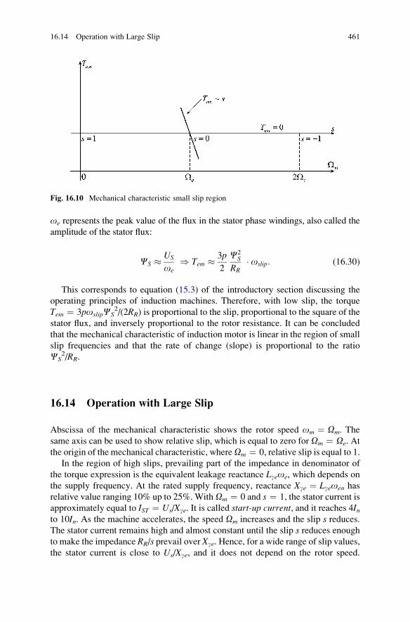
oe represents the peak value of the flux in the stator phase windings, also called the
amplitude of the stator flux:
CS � US
oe) Tem � 3p
2
C2S
RR oslip: (16.30)
This corresponds to equation (15.3) of the introductory section discussing the
operating principles of induction machines. Therefore, with low slip, the torque
Tem ¼ 3poslipCS2/(2RR) is proportional to the slip, proportional to the square of the
stator flux, and inversely proportional to the rotor resistance. It can be concluded
that the mechanical characteristic of induction motor is linear in the region of small
slip frequencies and that the rate of change (slope) is proportional to the ratio
CS2/RR.
16.14 Operation with Large Slip
Abscissa of the mechanical characteristic shows the rotor speed om ¼ Om. The
same axis can be used to show relative slip, which is equal to zero for Om ¼ Oe. At
the origin of the mechanical characteristic, whereOm ¼ 0, relative slip is equal to 1.
In the region of high slips, prevailing part of the impedance in denominator of
the torque expression is the equivalent leakage reactance Lgeoe, which depends on
the supply frequency. At the rated supply frequency, reactance Xge ¼ Lgeoen has
relative value ranging 10% up to 25%. With Om ¼ 0 and s ¼ 1, the stator current is
approximately equal to IST ¼ Us/Xge. It is called start-up current, and it reaches 4Into 10In. As the machine accelerates, the speed Om increases and the slip s reduces.The stator current remains high and almost constant until the slip s reduces enoughto make the impedance RR/s prevail over Xge. Hence, for a wide range of slip values,
the stator current is close to Us/Xge, and it does not depend on the rotor speed.
Fig. 16.10 Mechanical characteristic small slip region
16.14 Operation with Large Slip 461
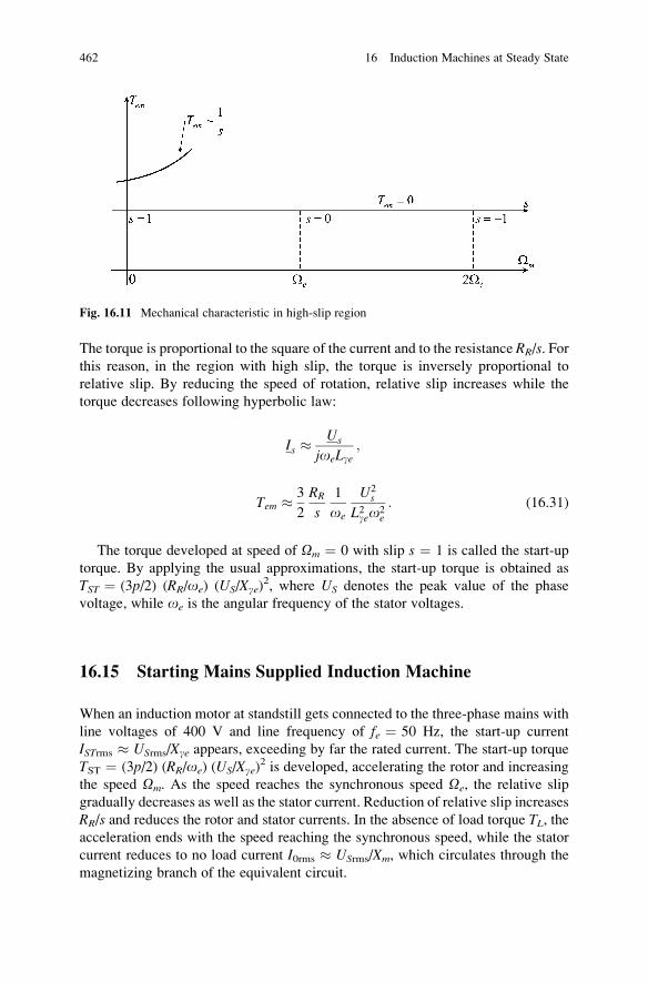
The torque is proportional to the square of the current and to the resistance RR/s. Forthis reason, in the region with high slip, the torque is inversely proportional to
relative slip. By reducing the speed of rotation, relative slip increases while the
torque decreases following hyperbolic law:
Is �Us
joeLge;
Tem � 3
2
RR
s
1
oe
U2s
L2geo2e
: (16.31)
The torque developed at speed of Om ¼ 0 with slip s ¼ 1 is called the start-up
torque. By applying the usual approximations, the start-up torque is obtained as
TST ¼ (3p/2) (RR/oe) (US/Xge)2, where US denotes the peak value of the phase
voltage, while oe is the angular frequency of the stator voltages.
16.15 Starting Mains Supplied Induction Machine
When an induction motor at standstill gets connected to the three-phase mains with
line voltages of 400 V and line frequency of fe ¼ 50 Hz, the start-up current
ISTrms � USrms/Xge appears, exceeding by far the rated current. The start-up torque
TST ¼ (3p/2) (RR/oe) (US/Xge)2 is developed, accelerating the rotor and increasing
the speed Om. As the speed reaches the synchronous speed Oe, the relative slip
gradually decreases as well as the stator current. Reduction of relative slip increases
RR/s and reduces the rotor and stator currents. In the absence of load torque TL, theacceleration ends with the speed reaching the synchronous speed, while the stator
current reduces to no load current I0rms � USrms/Xm, which circulates through the
magnetizing branch of the equivalent circuit.
Fig. 16.11 Mechanical characteristic in high-slip region
462 16 Induction Machines at Steady State
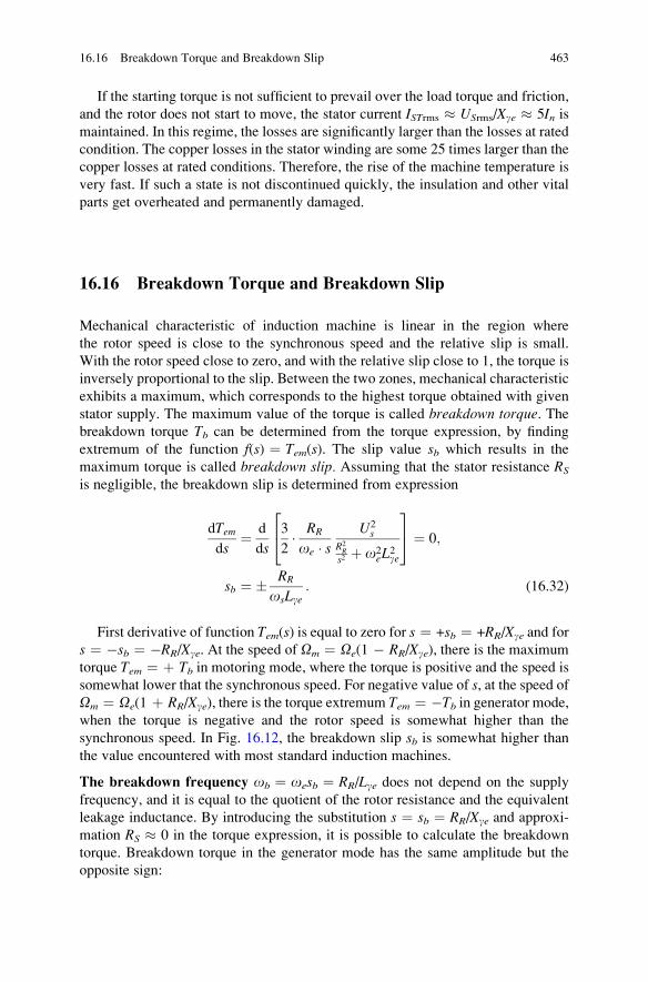
If the starting torque is not sufficient to prevail over the load torque and friction,
and the rotor does not start to move, the stator current ISTrms � USrms/Xge � 5In ismaintained. In this regime, the losses are significantly larger than the losses at rated
condition. The copper losses in the stator winding are some 25 times larger than the
copper losses at rated conditions. Therefore, the rise of the machine temperature is
very fast. If such a state is not discontinued quickly, the insulation and other vital
parts get overheated and permanently damaged.
16.16 Breakdown Torque and Breakdown Slip
Mechanical characteristic of induction machine is linear in the region where
the rotor speed is close to the synchronous speed and the relative slip is small.
With the rotor speed close to zero, and with the relative slip close to 1, the torque is
inversely proportional to the slip. Between the two zones, mechanical characteristic
exhibits a maximum, which corresponds to the highest torque obtained with given
stator supply. The maximum value of the torque is called breakdown torque. Thebreakdown torque Tb can be determined from the torque expression, by finding
extremum of the function f(s) ¼ Tem(s). The slip value sb which results in the
maximum torque is called breakdown slip. Assuming that the stator resistance RS
is negligible, the breakdown slip is determined from expression
dTemds
¼ d
ds
3
2 RR
oe sU2
sR2R
s2 þ o2eL
2ge
24
35 ¼ 0;
sb ¼ RR
osLge: (16.32)
First derivative of function Tem(s) is equal to zero for s ¼ +sb ¼ +RR/Xge and for
s ¼ �sb ¼ �RR/Xge. At the speed of Om ¼ Oe(1 � RR/Xge), there is the maximum
torque Tem ¼ þ Tb in motoring mode, where the torque is positive and the speed is
somewhat lower that the synchronous speed. For negative value of s, at the speed ofOm ¼ Oe(1 þ RR/Xge), there is the torque extremum Tem ¼ �Tb in generator mode,
when the torque is negative and the rotor speed is somewhat higher than the
synchronous speed. In Fig. 16.12, the breakdown slip sb is somewhat higher than
the value encountered with most standard induction machines.
The breakdown frequency ob ¼ oesb ¼ RR/Lge does not depend on the supply
frequency, and it is equal to the quotient of the rotor resistance and the equivalent
leakage inductance. By introducing the substitution s ¼ sb ¼ RR/Xge and approxi-
mation RS � 0 in the torque expression, it is possible to calculate the breakdown
torque. Breakdown torque in the generator mode has the same amplitude but the
opposite sign:
16.16 Breakdown Torque and Breakdown Slip 463
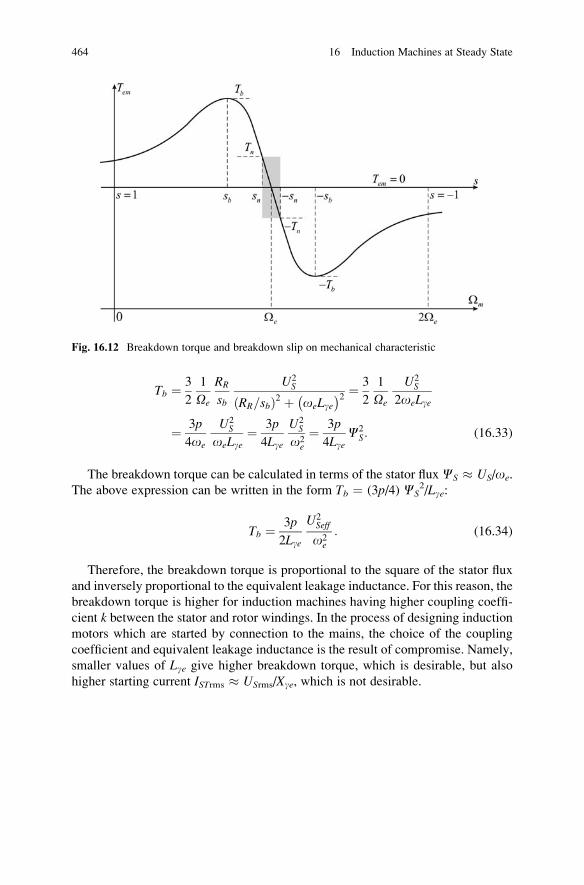
Tb ¼ 3
2
1
Oe
RR
sb
U2S
RR=sbð Þ2 þ oeLge� �2 ¼ 3
2
1
Oe
U2S
2oeLge
¼ 3p
4oe
U2S
oeLge¼ 3p
4Lge
U2S
o2e
¼ 3p
4LgeC2
S: (16.33)
The breakdown torque can be calculated in terms of the stator fluxCS � US/oe.
The above expression can be written in the form Tb ¼ (3p/4) CS2/Lge:
Tb ¼ 3p
2Lge
U2Seff
o2e
: (16.34)
Therefore, the breakdown torque is proportional to the square of the stator flux
and inversely proportional to the equivalent leakage inductance. For this reason, the
breakdown torque is higher for induction machines having higher coupling coeffi-
cient k between the stator and rotor windings. In the process of designing inductionmotors which are started by connection to the mains, the choice of the coupling
coefficient and equivalent leakage inductance is the result of compromise. Namely,
smaller values of Lge give higher breakdown torque, which is desirable, but also
higher starting current ISTrms � USrms/Xge, which is not desirable.
Fig. 16.12 Breakdown torque and breakdown slip on mechanical characteristic
464 16 Induction Machines at Steady State
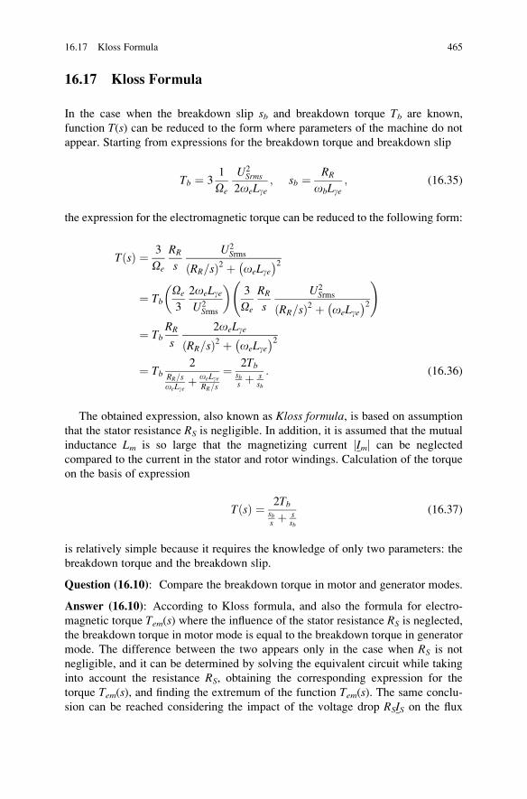
16.17 Kloss Formula
In the case when the breakdown slip sb and breakdown torque Tb are known,
function T(s) can be reduced to the form where parameters of the machine do not
appear. Starting from expressions for the breakdown torque and breakdown slip
Tb ¼ 31
Oe
U2Srms
2oeLge; sb ¼ RR
obLge; (16.35)
the expression for the electromagnetic torque can be reduced to the following form:
TðsÞ ¼ 3
Oe
RR
s
U2Srms
RR=sð Þ2 þ oeLge� �2
¼ TbOe
3
2oeLgeU2
Srms
� 3
Oe
RR
s
U2Srms
RR=sð Þ2 þ oeLge� �2
!
¼ TbRR
s
2oeLge
RR=sð Þ2 þ oeLge� �2
¼ Tb2
RR=soeLge
þ oeLgeRR=s
¼ 2Tbsbs þ s
sb
: (16.36)
The obtained expression, also known as Kloss formula, is based on assumption
that the stator resistance RS is negligible. In addition, it is assumed that the mutual
inductance Lm is so large that the magnetizing current jImj can be neglected
compared to the current in the stator and rotor windings. Calculation of the torque
on the basis of expression
TðsÞ ¼ 2Tbsbs þ s
sb
(16.37)
is relatively simple because it requires the knowledge of only two parameters: the
breakdown torque and the breakdown slip.
Question (16.10): Compare the breakdown torque in motor and generator modes.
Answer (16.10): According to Kloss formula, and also the formula for electro-
magnetic torque Tem(s) where the influence of the stator resistance RS is neglected,
the breakdown torque in motor mode is equal to the breakdown torque in generator
mode. The difference between the two appears only in the case when RS is not
negligible, and it can be determined by solving the equivalent circuit while taking
into account the resistance RS, obtaining the corresponding expression for the
torque Tem(s), and finding the extremum of the function Tem(s). The same conclu-
sion can be reached considering the impact of the voltage drop RSIS on the flux
16.17 Kloss Formula 465
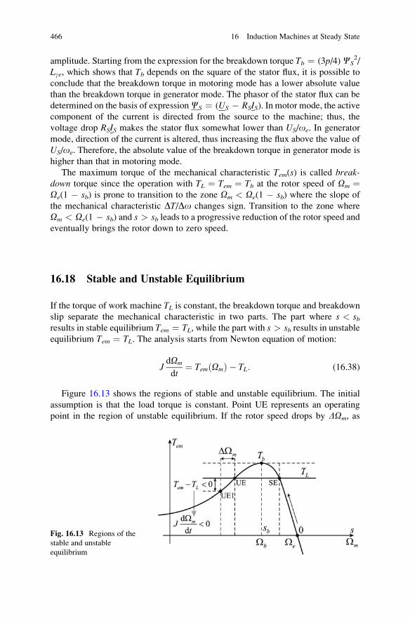
amplitude. Starting from the expression for the breakdown torque Tb ¼ (3p/4)CS2/
Lge, which shows that Tb depends on the square of the stator flux, it is possible to
conclude that the breakdown torque in motoring mode has a lower absolute value
than the breakdown torque in generator mode. The phasor of the stator flux can be
determined on the basis of expressionCS ¼ (US � RSIS). In motor mode, the active
component of the current is directed from the source to the machine; thus, the
voltage drop RSIS makes the stator flux somewhat lower than US/oe. In generator
mode, direction of the current is altered, thus increasing the flux above the value of
US/oe. Therefore, the absolute value of the breakdown torque in generator mode is
higher than that in motoring mode.
The maximum torque of the mechanical characteristic Tem(s) is called break-down torque since the operation with TL ¼ Tem ¼ Tb at the rotor speed of Om ¼Oe(1 � sb) is prone to transition to the zone Om < Oe(1 � sb) where the slope of
the mechanical characteristic DT/Do changes sign. Transition to the zone where
Om < Oe(1 � sb) and s > sb leads to a progressive reduction of the rotor speed andeventually brings the rotor down to zero speed.
16.18 Stable and Unstable Equilibrium
If the torque of work machine TL is constant, the breakdown torque and breakdownslip separate the mechanical characteristic in two parts. The part where s < sbresults in stable equilibrium Tem ¼ TL, while the part with s > sb results in unstableequilibrium Tem ¼ TL. The analysis starts from Newton equation of motion:
JdOm
dt¼ TemðOmÞ � TL: (16.38)
Figure 16.13 shows the regions of stable and unstable equilibrium. The initial
assumption is that the load torque is constant. Point UE represents an operating
point in the region of unstable equilibrium. If the rotor speed drops by DOm, as
Fig. 16.13 Regions of the
stable and unstable
equilibrium
466 16 Induction Machines at Steady State
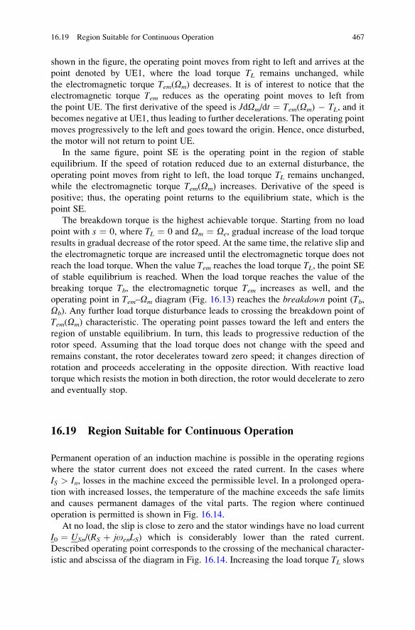
shown in the figure, the operating point moves from right to left and arrives at the
point denoted by UE1, where the load torque TL remains unchanged, while
the electromagnetic torque Tem(Om) decreases. It is of interest to notice that the
electromagnetic torque Tem reduces as the operating point moves to left from
the point UE. The first derivative of the speed is JdOm/dt ¼ Tem(Om) � TL, and it
becomes negative at UE1, thus leading to further decelerations. The operating point
moves progressively to the left and goes toward the origin. Hence, once disturbed,
the motor will not return to point UE.
In the same figure, point SE is the operating point in the region of stable
equilibrium. If the speed of rotation reduced due to an external disturbance, the
operating point moves from right to left, the load torque TL remains unchanged,
while the electromagnetic torque Tem(Om) increases. Derivative of the speed is
positive; thus, the operating point returns to the equilibrium state, which is the
point SE.
The breakdown torque is the highest achievable torque. Starting from no load
point with s ¼ 0, where TL ¼ 0 and Om ¼ Oe, gradual increase of the load torque
results in gradual decrease of the rotor speed. At the same time, the relative slip and
the electromagnetic torque are increased until the electromagnetic torque does not
reach the load torque. When the value Tem reaches the load torque TL, the point SEof stable equilibrium is reached. When the load torque reaches the value of the
breaking torque Tb, the electromagnetic torque Tem increases as well, and the
operating point in Tem–Om diagram (Fig. 16.13) reaches the breakdown point (Tb,Ob). Any further load torque disturbance leads to crossing the breakdown point of
Tem(Om) characteristic. The operating point passes toward the left and enters the
region of unstable equilibrium. In turn, this leads to progressive reduction of the
rotor speed. Assuming that the load torque does not change with the speed and
remains constant, the rotor decelerates toward zero speed; it changes direction of
rotation and proceeds accelerating in the opposite direction. With reactive load
torque which resists the motion in both direction, the rotor would decelerate to zero
and eventually stop.
16.19 Region Suitable for Continuous Operation
Permanent operation of an induction machine is possible in the operating regions
where the stator current does not exceed the rated current. In the cases where
IS > In, losses in the machine exceed the permissible level. In a prolonged opera-
tion with increased losses, the temperature of the machine exceeds the safe limits
and causes permanent damages of the vital parts. The region where continued
operation is permitted is shown in Fig. 16.14.
At no load, the slip is close to zero and the stator windings have no load current
I0 ¼ USn/(RS þ joenLS) which is considerably lower than the rated current.
Described operating point corresponds to the crossing of the mechanical character-
istic and abscissa of the diagram in Fig. 16.14. Increasing the load torque TL slows
16.19 Region Suitable for Continuous Operation 467
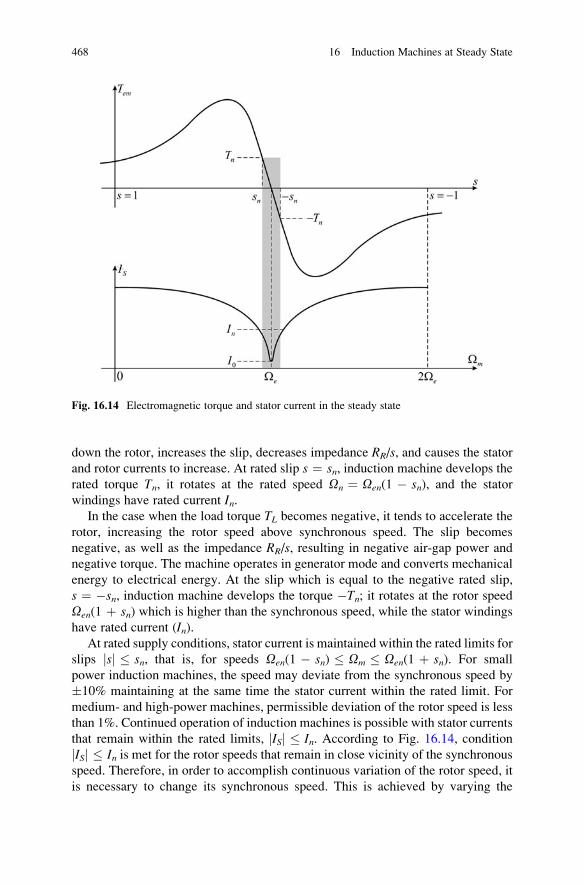
down the rotor, increases the slip, decreases impedance RR/s, and causes the stator
and rotor currents to increase. At rated slip s ¼ sn, induction machine develops the
rated torque Tn, it rotates at the rated speed On ¼ Oen(1 � sn), and the stator
windings have rated current In.In the case when the load torque TL becomes negative, it tends to accelerate the
rotor, increasing the rotor speed above synchronous speed. The slip becomes
negative, as well as the impedance RR/s, resulting in negative air-gap power and
negative torque. The machine operates in generator mode and converts mechanical
energy to electrical energy. At the slip which is equal to the negative rated slip,
s ¼ �sn, induction machine develops the torque �Tn; it rotates at the rotor speed
Oen(1 þ sn) which is higher than the synchronous speed, while the stator windings
have rated current (In).At rated supply conditions, stator current is maintained within the rated limits for
slips jsj � sn, that is, for speeds Oen(1 � sn) � Om � Oen(1 þ sn). For small
power induction machines, the speed may deviate from the synchronous speed by
10% maintaining at the same time the stator current within the rated limit. For
medium- and high-power machines, permissible deviation of the rotor speed is less
than 1%. Continued operation of induction machines is possible with stator currents
that remain within the rated limits, jISj � In. According to Fig. 16.14, condition
jISj � In is met for the rotor speeds that remain in close vicinity of the synchronous
speed. Therefore, in order to accomplish continuous variation of the rotor speed, it
is necessary to change its synchronous speed. This is achieved by varying the
Fig. 16.14 Electromagnetic torque and stator current in the steady state
468 16 Induction Machines at Steady State
frequency of the stator voltages and currents, which is achieved by supplying the
induction machine from a three-phase source providing variable frequency AC
voltages.
16.20 Losses and Power Balance
One of the assumptions taken in modeling of electrical machines has been
neglecting the losses in magnetic circuit, also called iron losses. These losses
have one part proportional to B2f 2, caused by eddy currents, and the other part
proportional to B2f, caused by hysteresis of the B(H) curve. The power balance
discussed hereafter takes into account the iron losses as well.
Within the rotor of an induction machine, there are variations of the magnetic
induction at relatively low-slip frequency. Thus, the power of losses within the rotor
magnetic circuit is relatively small. Power of iron losses in the stator magnetic
circuit is considerably higher since the magnetic field in the stator core varies at the
frequency of the supply voltages oe. Besides iron losses and copper losses, the
process of electromechanical conversion has the losses in mechanical subsystem.
Mechanical losses include the motion resistances such as the air resistance and
friction in bearings.
16.21 Copper, Iron, and Mechanical Losses
The most significant losses in an induction machine are:
• Copper losses in stator windings, RSIS2
• Losses in rotor cage winding, RRIR2
• Iron losses in stator magnetic circuit, sH fe Bm2 þ sV fe
2 Bm2
• Iron losses in rotor magnetic circuit, sH fk Bm2 þ sV fk
2 Bm2
• Mechanical losses due to rotation, kFOm2
Losses in copper of the stator winding are proportional to the square of the rms
value of the stator current, Pcu1 ¼ 3RS ISrms2.
The losses PFe1 in stator magnetic circuit are proportional to square of the
magnetic induction, and they are dependent on stator frequency fe. If the eddy
current losses prevail, the iron losses are proportional to the square of the stator
frequency.
Currents in rotor bars create losses which are proportional to the square of the
rotor current, PCu2 ¼ 3RRIRrms2. In addition to losses in the rotor winding, there are
also iron losses in the rotor magnetic circuit, where the magnetic field varies at the
slip frequency oslip. The slip frequency oslip is much lower than the stator fre-
quency. Therefore, the rotor iron losses are often neglected. Yet, there are operating
modes where the rotor iron losses are considerable and cannot be neglected. One of
16.21 Copper, Iron, and Mechanical Losses 469
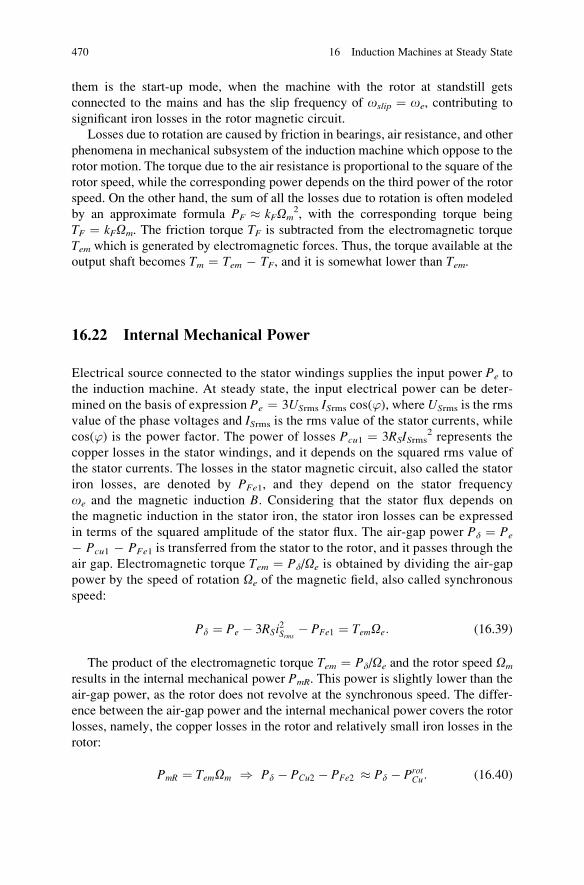
them is the start-up mode, when the machine with the rotor at standstill gets
connected to the mains and has the slip frequency of oslip ¼ oe, contributing to
significant iron losses in the rotor magnetic circuit.
Losses due to rotation are caused by friction in bearings, air resistance, and other
phenomena in mechanical subsystem of the induction machine which oppose to the
rotor motion. The torque due to the air resistance is proportional to the square of the
rotor speed, while the corresponding power depends on the third power of the rotor
speed. On the other hand, the sum of all the losses due to rotation is often modeled
by an approximate formula PF � kFOm2, with the corresponding torque being
TF ¼ kFOm. The friction torque TF is subtracted from the electromagnetic torque
Tem which is generated by electromagnetic forces. Thus, the torque available at the
output shaft becomes Tm ¼ Tem � TF, and it is somewhat lower than Tem.
16.22 Internal Mechanical Power
Electrical source connected to the stator windings supplies the input power Pe to
the induction machine. At steady state, the input electrical power can be deter-
mined on the basis of expression Pe ¼ 3USrms ISrms cos(’), where USrms is the rms
value of the phase voltages and ISrms is the rms value of the stator currents, while
cos(’) is the power factor. The power of losses Pcu1 ¼ 3RSISrms2 represents the
copper losses in the stator windings, and it depends on the squared rms value of
the stator currents. The losses in the stator magnetic circuit, also called the stator
iron losses, are denoted by PFe1, and they depend on the stator frequency
oe and the magnetic induction B. Considering that the stator flux depends on
the magnetic induction in the stator iron, the stator iron losses can be expressed
in terms of the squared amplitude of the stator flux. The air-gap power Pd ¼ Pe
� Pcu1 � PFe1 is transferred from the stator to the rotor, and it passes through the
air gap. Electromagnetic torque Tem ¼ Pd/Oe is obtained by dividing the air-gap
power by the speed of rotation Oe of the magnetic field, also called synchronous
speed:
Pd ¼ Pe � 3RSi2Srms
� PFe1 ¼ TemOe: (16.39)
The product of the electromagnetic torque Tem ¼ Pd/Oe and the rotor speed Om
results in the internal mechanical power PmR. This power is slightly lower than the
air-gap power, as the rotor does not revolve at the synchronous speed. The differ-
ence between the air-gap power and the internal mechanical power covers the rotor
losses, namely, the copper losses in the rotor and relatively small iron losses in the
rotor:
PmR ¼ TemOm ) Pd � PCu2 � PFe2 � Pd � ProtCu: (16.40)
470 16 Induction Machines at Steady State
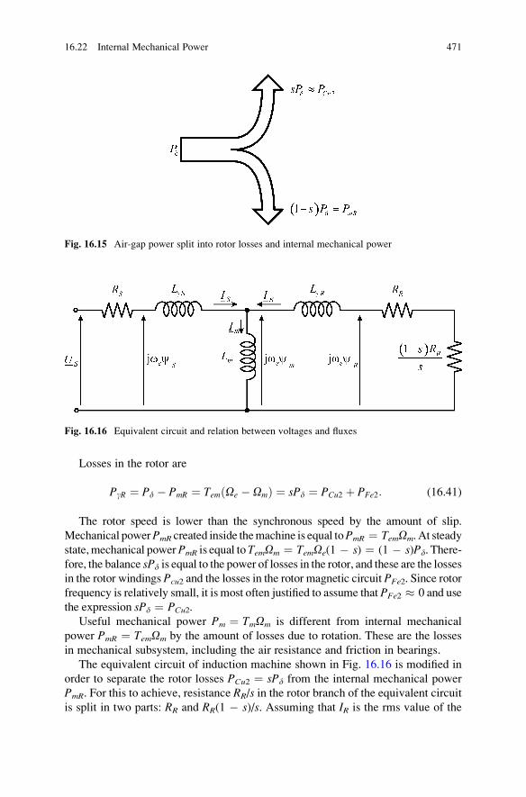
Losses in the rotor are
PgR ¼ Pd � PmR ¼ TemðOe � OmÞ ¼ sPd ¼ PCu2 þ PFe2: (16.41)
The rotor speed is lower than the synchronous speed by the amount of slip.
Mechanical powerPmR created inside themachine is equal toPmR ¼ TemOm. At steady
state,mechanical powerPmR is equal toTemOm ¼ TemOe(1 � s) ¼ (1 � s)Pd. There-
fore, the balance sPd is equal to the power of losses in the rotor, and these are the losses
in the rotor windings Pcu2 and the losses in the rotor magnetic circuit PFe2. Since rotor
frequency is relatively small, it is most often justified to assume that PFe2 � 0 and use
the expression sPd ¼ PCu2.
Useful mechanical power Pm ¼ TmOm is different from internal mechanical
power PmR ¼ TemOm by the amount of losses due to rotation. These are the losses
in mechanical subsystem, including the air resistance and friction in bearings.
The equivalent circuit of induction machine shown in Fig. 16.16 is modified in
order to separate the rotor losses PCu2 ¼ sPd from the internal mechanical power
PmR. For this to achieve, resistance RR/s in the rotor branch of the equivalent circuitis split in two parts: RR and RR(1 � s)/s. Assuming that IR is the rms value of the
Fig. 16.15 Air-gap power split into rotor losses and internal mechanical power
Fig. 16.16 Equivalent circuit and relation between voltages and fluxes
16.22 Internal Mechanical Power 471
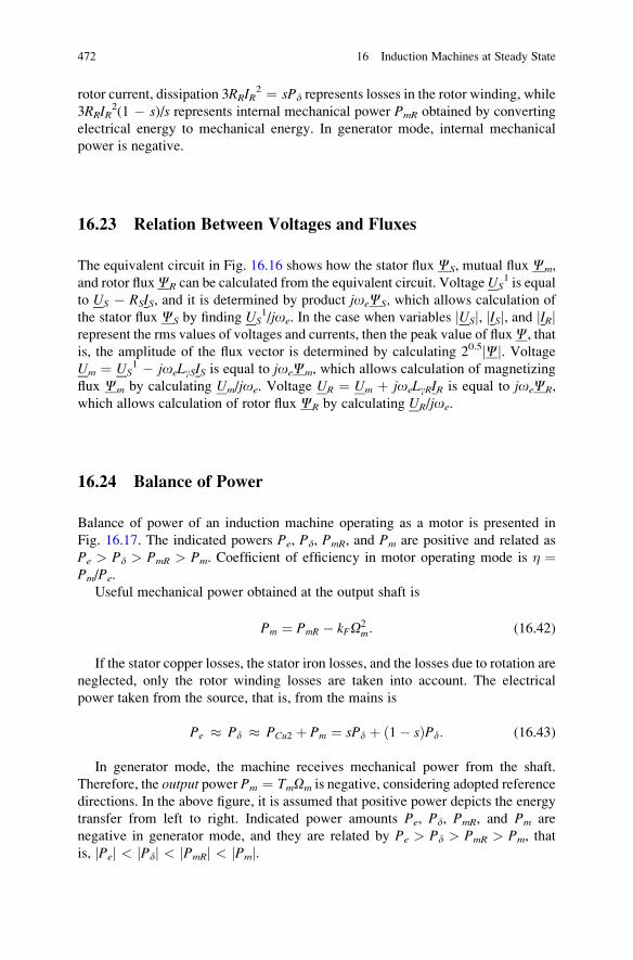
rotor current, dissipation 3RRIR2 ¼ sPd represents losses in the rotor winding, while
3RRIR2(1 � s)/s represents internal mechanical power PmR obtained by converting
electrical energy to mechanical energy. In generator mode, internal mechanical
power is negative.
16.23 Relation Between Voltages and Fluxes
The equivalent circuit in Fig. 16.16 shows how the stator flux CS, mutual flux Cm,
and rotor fluxCR can be calculated from the equivalent circuit. VoltageUS1 is equal
to US � RSIS, and it is determined by product joeCS, which allows calculation of
the stator flux CS by finding US1/joe. In the case when variables jUSj, jISj, and jIRj
represent the rms values of voltages and currents, then the peak value of fluxC, that
is, the amplitude of the flux vector is determined by calculating 20.5jCj. VoltageUm ¼ US
1 � joeLgSIS is equal to joeCm, which allows calculation of magnetizing
flux Cm by calculating Um/joe. Voltage UR ¼ Um þ joeLgRIR is equal to joeCR,
which allows calculation of rotor flux CR by calculating UR/joe.
16.24 Balance of Power
Balance of power of an induction machine operating as a motor is presented in
Fig. 16.17. The indicated powers Pe, Pd, PmR, and Pm are positive and related as
Pe > Pd > PmR > Pm. Coefficient of efficiency in motor operating mode is � ¼Pm/Pe.
Useful mechanical power obtained at the output shaft is
Pm ¼ PmR � kFO2m: (16.42)
If the stator copper losses, the stator iron losses, and the losses due to rotation are
neglected, only the rotor winding losses are taken into account. The electrical
power taken from the source, that is, from the mains is
Pe � Pd � PCu2 þ Pm ¼ sPd þ 1� sð ÞPd: (16.43)
In generator mode, the machine receives mechanical power from the shaft.
Therefore, the output power Pm ¼ TmOm is negative, considering adopted reference
directions. In the above figure, it is assumed that positive power depicts the energy
transfer from left to right. Indicated power amounts Pe, Pd, PmR, and Pm are
negative in generator mode, and they are related by Pe > Pd > PmR > Pm, that
is, jPej < jPdj < jPmRj < jPmj.
472 16 Induction Machines at Steady State
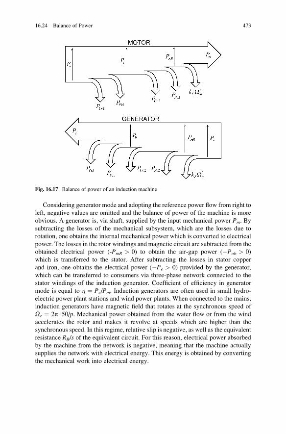
Considering generator mode and adopting the reference power flow from right to
left, negative values are omitted and the balance of power of the machine is more
obvious. A generator is, via shaft, supplied by the input mechanical power Pm. By
subtracting the losses of the mechanical subsystem, which are the losses due to
rotation, one obtains the internal mechanical power which is converted to electrical
power. The losses in the rotor windings and magnetic circuit are subtracted from the
obtained electrical power (-PmR > 0) to obtain the air-gap power (�Pob > 0)
which is transferred to the stator. After subtracting the losses in stator copper
and iron, one obtains the electrical power (�Pe > 0) provided by the generator,
which can be transferred to consumers via three-phase network connected to the
stator windings of the induction generator. Coefficient of efficiency in generator
mode is equal to � ¼ Pe/Pm. Induction generators are often used in small hydro-
electric power plant stations and wind power plants. When connected to the mains,
induction generators have magnetic field that rotates at the synchronous speed of
Oe ¼ 2p ∙50/p. Mechanical power obtained from the water flow or from the wind
accelerates the rotor and makes it revolve at speeds which are higher than the
synchronous speed. In this regime, relative slip is negative, as well as the equivalent
resistance RR/s of the equivalent circuit. For this reason, electrical power absorbedby the machine from the network is negative, meaning that the machine actually
supplies the network with electrical energy. This energy is obtained by converting
the mechanical work into electrical energy.
Fig. 16.17 Balance of power of an induction machine
16.24 Balance of Power 473
Chapter 17
Variable Speed Induction Machines
This chapter discusses the means for the speed change of induction machines.
The speed regulation is required in both generators and motors. Induction machines
that serve as generators in wind power stations revolve at variable speed. Therefore,
the machine and the associated equipment must ensure conversion of mechanical
work in electrical energy at variable speed. The machines used as motors often serve
in motion control applications, where the speed changes in continuous manner.
In the first part of this chapter, the means for altering the rotor speed of mains-
supplied induction machines are discussed and explained. Possibilities are consid-
ered to adjust the rotor speed of induction machines operating with constant
frequency of stator voltages. The analysis considers changes in mechanical charac-
teristic and the rotor speed due to variations of the voltage amplitude. Variation of
the rotor resistance is studied as the means of changing the rotor speed of wound
rotor induction machines. The impact of the number of magnetic pole pairs p on
synchronous speed Oe and rotor speed Om is reinstated, and the change of the
number of poles is looked upon as the means of changing the rotor speed.
An introduction to electrical machines with multiple pole pairs is given by studying
distribution of the magnetic field of an electrical machine with 2p ¼ 4 magnetic
poles. The possibility of designing the stator winding so as to achieve the magnetic
field with multiple pole pairs is studied on a sample winding that can be switched to
produce either 2p ¼ 2 poles or 2p ¼ 4 poles. The expressions for synchronous
speed, rotor speed, and slip frequency are given as functions of the number of
magnetic pole pairs. Discussion on constant frequency-supplied induction machine
closes with establishing deficiencies, limitations, energy losses, and design
problems arising in mains-supplied induction machines.
The second part of this chapter deals with induction machines supplied from
variable frequency sources such as the three-phase inverters with switching power
transistors and pulse width modulation control. This chapter introduces basic
aspects and problems of variable frequency supply. Operation of induction
machines fed from variable frequency static power converter is introduced and
studied. A short review of power converter topologies used for supplying induction
machines is presented, along with methods for continuous change in the stator
S.N. Vukosavic, Electrical Machines, Power Electronics and Power Systems,
DOI 10.1007/978-1-4614-0400-2_17, # Springer Science+Business Media New York 2013
475
voltage amplitude and frequency, suited to accomplish desired rotor speed and
desired flux. The effects of changing the supply frequency on mechanical charac-
teristic are analyzed in both the constant flux region and in the field weakening
region. The basic approaches the torque, flux, and power control are outlined for an
induction machine fed from a variable frequency static power converter. Family of
mechanical characteristics obtained by frequency variation is presented and
explained. Based upon the study of operating limits of the machine and operating
limits of associated three-phase inverter, steady state operating area and transient
operating area are derived in T-O plane and studied for variable frequency operation
of induction machines. The limits of constant power operation in field weakening
mode are determined, explained, and expressed in terms of the machine leakage
inductance. Finally, this chapter discusses the differences in construction and
parameters of mains-supplied induction machines and inverter-supplied induction
machines.
17.1 Speed Changes in Mains-Supplied Machines
In majority of applications of electrical machines, it is required to accomplish a
continuous variation of the rotor speed. Some of examples are motion control tasks
in production machines and industrial robots and propulsion tasks in electrical
vehicles, fans, pumps, and similar.
The rotor speed of induction machines is different from the synchronous speed
by the amount of the slip. When an induction motor is supplied from the mains, the
stator current is maintained within rated limits under condition that the slip remains
relatively low, jsj � sn, namely, for the speed range Oen(1� sn) � Om � Oen(1 þsn). Hence, continuous operation of mains-supplied induction machine is restricted
to a rather narrow range of speeds. For medium- and high-power machines, the
rated slip is lower than 1%; thus, the condition IS � In is maintained within the
range of speeds from 99% up to 101% of the synchronous speed. Operation at
higher slip frequencies involves high losses and high currents in stator and rotor
windings. The use of induction machine outside the zone where jsj � sn and IS � Inleads to an increase of the machine temperature. For this reason, continued service
of induction machines is possible only with relatively small values of slip. There-
fore, it is justified to conclude that the speed of rotation Om is close to the
synchronous speed Oe. Synchronous speed Oe ¼ oe/p is determined by the angular
frequency of the stator voltages oe, that is, by the frequency of electrical currents in
stator windings. For two-pole machines, where the number of pole pairs p is equal
to 1, the synchronous speed is equal to the angular frequency of the supply. For this
reason, variation of the rotor speed of an induction machine requires a variable
frequency of the stator voltages and currents. This can be accomplished by supply-
ing the machine from a three-phase source of AC voltages having variable
frequency. Most common solution to this is the three-phase inverter, a power
converter which employs semiconductor power switches. Inverters are mostly
476 17 Variable Speed Induction Machines
used in conjunction with three-phase diode rectifiers. Three-phase diode rectifiers
are power converters supplied from the mains with line voltages of 400 V and line
frequency of f ¼ 50 or 60 Hz. The rectifier converts the AC line voltages into DC
voltage. This DC voltage is fed to the three-phase inverter, which converts the
DC voltage into a set of three-phase AC voltage of variable frequency and variable
amplitude. Finally, at the output terminals of the inverter, a three-phase system is
available with frequency and voltage amplitude that can be changed to suit the
needs of the induction machine. Contemporary inverters apply pulse width modu-
lation control and make use of semiconductor switches such as bipolar transistors
(BJT), MOSFET transistors, and IGBT transistors. Industrial use of such devices
started in last decades of the twentieth century. At present, power converters using
power transistors are standard industrial units for supplying induction machines and
changing their speed (Fig. 17.10a).
Induction machines have been in use for more than 100 years. During the first
century of industrial use of induction machines, there were no semiconductor
switches suitable for designing the three-phase inverters. Therefore, another kind
of components, devices, and techniques was being devised and used to achieve
continuous variation of the rotor speed of induction machines. Induction machines
were supplied from the mains providing the voltages of industrial frequency,
whether fe ¼ 50 Hz or fe ¼ 60 Hz. There were no ways of altering the supply
frequency and providing continuous change of the synchronous speed. Therefore,
most induction machines were primarily used in constant speed applications.
Particular procedures, methods, and devices were used in applications requiring
variable speed operation, all of them conditioned and restricted by technology
limits of the times. Traditional approaches to speed variations include:
1. Variation of stator voltage
2. Variation of rotor resistance
3. Variation of the number of poles
Besides, in some cases, induction motors were connected to mechanical load by
means of transmission mechanism with gears or some other mechanical
transducers. Using particularly suited transmission with variable transmission
ratio, it was possible to change the load speed while the induction motor speed
remained constant, close to the synchronous speed.
In further text, the effects of the traditional approaches (1), (2), and (3) will be
reviewed.
17.2 Voltage Change
With constant frequency supply, mechanical characteristic of an induction machine
crosses the abscissa Om of Tem�Om plane at Om ¼ Oe ¼2pfe/p, where Tem ¼ 0
(Fig. 17.1). Upon loading, the slip increases and the speed decreases. In generator
mode, where Tem < 0 and oslip < 0, the torque amplitude jTemj increases as the
17.2 Voltage Change 477
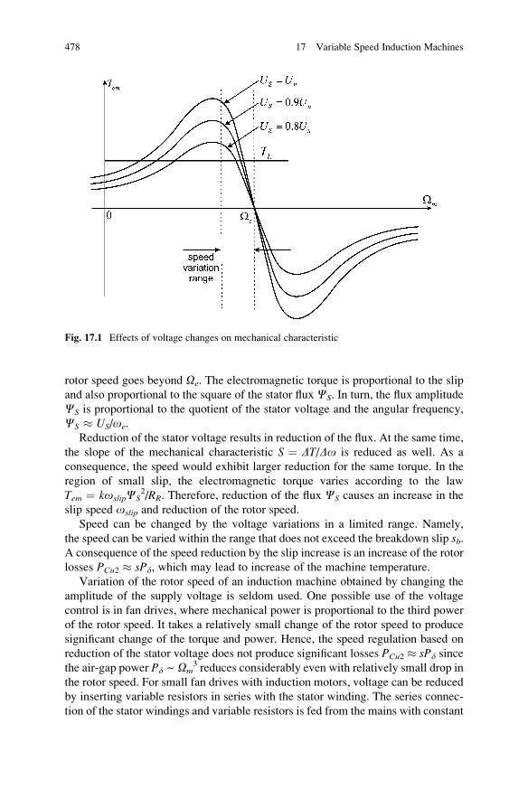
rotor speed goes beyond Oe. The electromagnetic torque is proportional to the slip
and also proportional to the square of the stator flux CS. In turn, the flux amplitude
CS is proportional to the quotient of the stator voltage and the angular frequency,
CS � US/oe.
Reduction of the stator voltage results in reduction of the flux. At the same time,
the slope of the mechanical characteristic S ¼ DT/Do is reduced as well. As a
consequence, the speed would exhibit larger reduction for the same torque. In the
region of small slip, the electromagnetic torque varies according to the law
Tem ¼ koslipCS2/RR. Therefore, reduction of the flux CS causes an increase in the
slip speed oslip and reduction of the rotor speed.
Speed can be changed by the voltage variations in a limited range. Namely,
the speed can be varied within the range that does not exceed the breakdown slip sb.A consequence of the speed reduction by the slip increase is an increase of the rotor
losses PCu2 � sPd, which may lead to increase of the machine temperature.
Variation of the rotor speed of an induction machine obtained by changing the
amplitude of the supply voltage is seldom used. One possible use of the voltage
control is in fan drives, where mechanical power is proportional to the third power
of the rotor speed. It takes a relatively small change of the rotor speed to produce
significant change of the torque and power. Hence, the speed regulation based on
reduction of the stator voltage does not produce significant losses PCu2 � sPd since
the air-gap power Pd ~ Om3 reduces considerably even with relatively small drop in
the rotor speed. For small fan drives with induction motors, voltage can be reduced
by inserting variable resistors in series with the stator winding. The series connec-
tion of the stator windings and variable resistors is fed from the mains with constant
Fig. 17.1 Effects of voltage changes on mechanical characteristic
478 17 Variable Speed Induction Machines
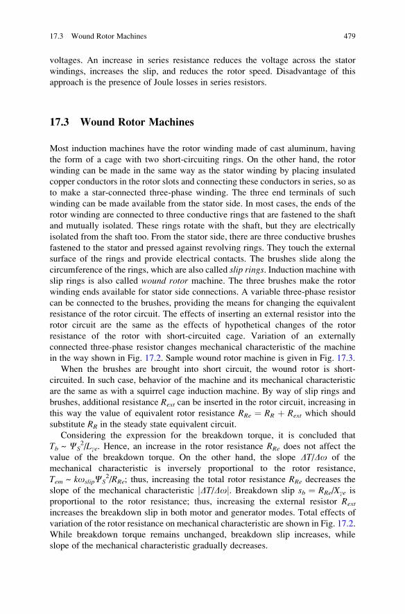
voltages. An increase in series resistance reduces the voltage across the stator
windings, increases the slip, and reduces the rotor speed. Disadvantage of this
approach is the presence of Joule losses in series resistors.
17.3 Wound Rotor Machines
Most induction machines have the rotor winding made of cast aluminum, having
the form of a cage with two short-circuiting rings. On the other hand, the rotor
winding can be made in the same way as the stator winding by placing insulated
copper conductors in the rotor slots and connecting these conductors in series, so as
to make a star-connected three-phase winding. The three end terminals of such
winding can be made available from the stator side. In most cases, the ends of the
rotor winding are connected to three conductive rings that are fastened to the shaft
and mutually isolated. These rings rotate with the shaft, but they are electrically
isolated from the shaft too. From the stator side, there are three conductive brushes
fastened to the stator and pressed against revolving rings. They touch the external
surface of the rings and provide electrical contacts. The brushes slide along the
circumference of the rings, which are also called slip rings. Induction machine with
slip rings is also called wound rotor machine. The three brushes make the rotor
winding ends available for stator side connections. A variable three-phase resistor
can be connected to the brushes, providing the means for changing the equivalent
resistance of the rotor circuit. The effects of inserting an external resistor into the
rotor circuit are the same as the effects of hypothetical changes of the rotor
resistance of the rotor with short-circuited cage. Variation of an externally
connected three-phase resistor changes mechanical characteristic of the machine
in the way shown in Fig. 17.2. Sample wound rotor machine is given in Fig. 17.3.
When the brushes are brought into short circuit, the wound rotor is short-
circuited. In such case, behavior of the machine and its mechanical characteristic
are the same as with a squirrel cage induction machine. By way of slip rings and
brushes, additional resistance Rext can be inserted in the rotor circuit, increasing in
this way the value of equivalent rotor resistance RRe ¼ RR þ Rext which should
substitute RR in the steady state equivalent circuit.
Considering the expression for the breakdown torque, it is concluded that
Tb ~ CS2/Lge. Hence, an increase in the rotor resistance RRe does not affect the
value of the breakdown torque. On the other hand, the slope DT/Do of the
mechanical characteristic is inversely proportional to the rotor resistance,
Tem ~ koslipCS2/RRe; thus, increasing the total rotor resistance RRe decreases the
slope of the mechanical characteristic jDT/Doj. Breakdown slip sb ¼ RRe/Xge is
proportional to the rotor resistance; thus, increasing the external resistor Rext
increases the breakdown slip in both motor and generator modes. Total effects of
variation of the rotor resistance on mechanical characteristic are shown in Fig. 17.2.
While breakdown torque remains unchanged, breakdown slip increases, while
slope of the mechanical characteristic gradually decreases.
17.3 Wound Rotor Machines 479
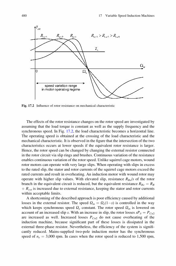
The effects of the rotor resistance changes on the rotor speed are investigated by
assuming that the load torque is constant as well as the supply frequency and the
synchronous speed. In Fig. 17.2, the load characteristic becomes a horizontal line.
The operating speed is obtained at the crossing of the load characteristic and the
mechanical characteristic. It is observed in the figure that the intersection of the two
characteristics occurs at lower speeds if the equivalent rotor resistance is larger.
Hence, the rotor speed can be changed by changing the external resistor connected
in the rotor circuit via slip rings and brushes. Continuous variation of the resistance
enables continuous variation of the rotor speed. Unlike squirrel cage motors, wound
rotor motors can operate with very large slips. When operating with slips in excess
to the rated slip, the stator and rotor currents of the squirrel cage motors exceed the
rated currents and result in overheating. An induction motor with wound rotor may
operate with higher slip values. With elevated slip, resistance RRe/s of the rotor
branch in the equivalent circuit is reduced, but the equivalent resistance RRe ¼ RR
þ Rext is increased due to external resistance, keeping the stator and rotor currents
within acceptable limits.
A shortcoming of the described approach is poor efficiency caused by additional
losses in the external resistor. The speed Om ¼ Oe(1�s) is controlled in the way
which keeps synchronous speed Oe constant. The rotor speed Om is lowered on
account of an increased slip s. With an increase in slip, the rotor losses sPd ¼ PCu2
are increased as well. Increased losses PCu2 do not cause overheating of the
induction machine, because significant part of these losses is dissipated in the
external three-phase resistor. Nevertheless, the efficiency of the system is signifi-
cantly reduced. Mains-supplied two-pole induction motor has the synchronous
speed of ne ¼ 3,000 rpm. In cases when the rotor speed is reduced to 1,500 rpm,
Fig. 17.2 Influence of rotor resistance on mechanical characteristic
480 17 Variable Speed Induction Machines
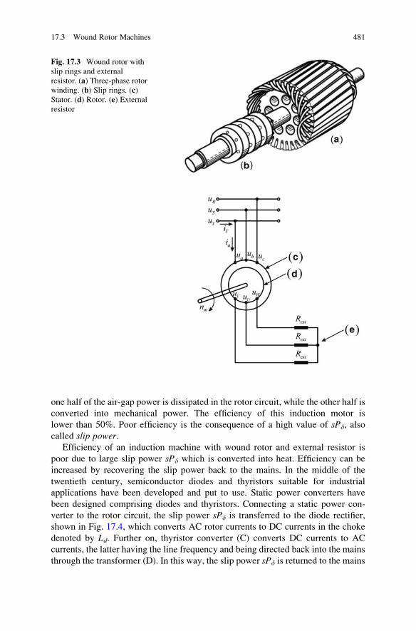
one half of the air-gap power is dissipated in the rotor circuit, while the other half is
converted into mechanical power. The efficiency of this induction motor is
lower than 50%. Poor efficiency is the consequence of a high value of sPd, also
called slip power.Efficiency of an induction machine with wound rotor and external resistor is
poor due to large slip power sPd which is converted into heat. Efficiency can be
increased by recovering the slip power back to the mains. In the middle of the
twentieth century, semiconductor diodes and thyristors suitable for industrial
applications have been developed and put to use. Static power converters have
been designed comprising diodes and thyristors. Connecting a static power con-
verter to the rotor circuit, the slip power sPd is transferred to the diode rectifier,
shown in Fig. 17.4, which converts AC rotor currents to DC currents in the choke
denoted by Ld. Further on, thyristor converter (C) converts DC currents to AC
currents, the latter having the line frequency and being directed back into the mains
through the transformer (D). In this way, the slip power sPd is returned to the mains
Fig. 17.3 Wound rotor with
slip rings and external
resistor. (a) Three-phase rotor
winding. (b) Slip rings. (c)
Stator. (d) Rotor. (e) External
resistor
17.3 Wound Rotor Machines 481
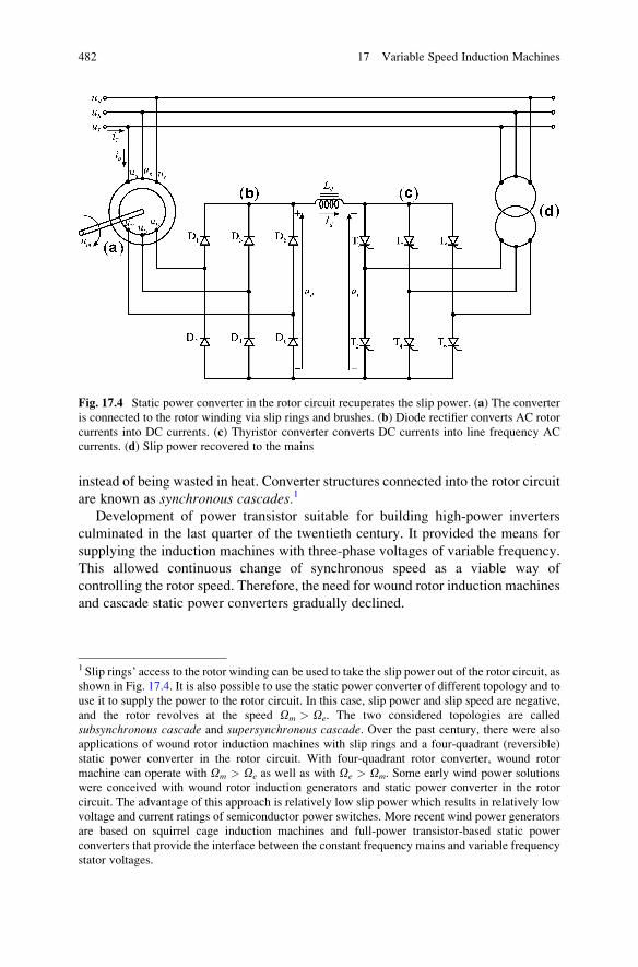
instead of being wasted in heat. Converter structures connected into the rotor circuit
are known as synchronous cascades.1
Development of power transistor suitable for building high-power inverters
culminated in the last quarter of the twentieth century. It provided the means for
supplying the induction machines with three-phase voltages of variable frequency.
This allowed continuous change of synchronous speed as a viable way of
controlling the rotor speed. Therefore, the need for wound rotor induction machines
and cascade static power converters gradually declined.
Fig. 17.4 Static power converter in the rotor circuit recuperates the slip power. (a) The converter
is connected to the rotor winding via slip rings and brushes. (b) Diode rectifier converts AC rotor
currents into DC currents. (c) Thyristor converter converts DC currents into line frequency AC
currents. (d) Slip power recovered to the mains
1 Slip rings’ access to the rotor winding can be used to take the slip power out of the rotor circuit, as
shown in Fig. 17.4. It is also possible to use the static power converter of different topology and to
use it to supply the power to the rotor circuit. In this case, slip power and slip speed are negative,
and the rotor revolves at the speed Om > Oe. The two considered topologies are called
subsynchronous cascade and supersynchronous cascade. Over the past century, there were also
applications of wound rotor induction machines with slip rings and a four-quadrant (reversible)
static power converter in the rotor circuit. With four-quadrant rotor converter, wound rotor
machine can operate with Om > Oe as well as with Oe > Om. Some early wind power solutions
were conceived with wound rotor induction generators and static power converter in the rotor
circuit. The advantage of this approach is relatively low slip power which results in relatively low
voltage and current ratings of semiconductor power switches. More recent wind power generators
are based on squirrel cage induction machines and full-power transistor-based static power
converters that provide the interface between the constant frequency mains and variable frequency
stator voltages.
482 17 Variable Speed Induction Machines
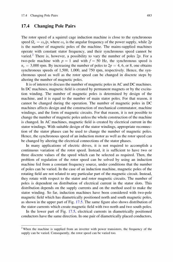
17.4 Changing Pole Pairs
The rotor speed of a squirrel cage induction machine is close to the synchronous
speed Oe ¼ oe/p, where oe is the angular frequency of the power supply, while 2pis the number of magnetic poles of the machine. The mains-supplied machines
operate with constant stator frequency, and their synchronous speed cannot be
varied.2 There is, however, a possibility to vary the number of poles 2p. For atwo-pole machine with p ¼ 1 and with f ¼ 50 Hz, the synchronous speed is
ne ¼ 3,000 rpm. By increasing the number of poles to 2p ¼ 4, 6, or 8, one obtains
synchronous speeds of 1,500, 1,000, and 750 rpm, respectively. Hence, the syn-
chronous speed as well as the rotor speed can be changed in discrete steps by
altering the number of magnetic poles.
It is of interest to discuss the number of magnetic poles in AC and DC machines.
In DC machines, magnetic field is created by permanent magnets or by the excita-
tion winding. The number of magnetic poles is determined by design of the
machine, and it is equal to the number of main stator poles. For that reason, it
cannot be changed during the operation. The number of magnetic poles in DC
machines affects design and the construction of mechanical commutator, machine
windings, and the form of magnetic circuits. For that reason, it is not possible to
change the number of magnetic poles unless the whole construction of the machine
is changed. In AC machines, magnetic field is created by electrical current in the
stator windings. With suitable design of the stator windings, appropriate reconnec-
tion of the stator phases can be used to change the number of magnetic poles.
Hence, the synchronous speed of an induction motor as well as the rotor speed can
be changed by altering the electrical connections of the stator phases.
In many applications of electric drives, it is not required to accomplish a
continuous variation of the rotor speed. Instead, it is sufficient to have two or
three discrete values of the speed which can be selected as required. Then, the
problem of regulation of the rotor speed can be solved by using an induction
machine fed from a constant frequency source, under conditions that the number
of poles can be varied. In the case of an induction machine, magnetic poles of the
rotating field are not related to any particular part of the magnetic circuit. Instead,
they rotate with respect to the stator and rotor magnetic circuits. The number of
poles is dependent on distribution of electrical current in the stator slots. This
distribution depends on the supply currents and on the method used to make the
stator winding. So far, induction machines have been considered with two-pole
magnetic field which has diametrically positioned north and south magnetic poles,
as shown in the upper part of Fig. 17.5. The same figure also shows distribution of
the stator currents which create magnetic field with two north and two south poles.
In the lower part of Fig. 17.5, electrical currents in diametrically positioned
conductors have the same direction. In one pair of diametrically placed conductors,
2When the machine is supplied from an inverter with power transistors, the frequency of the
supply can be varied. Consequently, the rotor speed can be varied too.
17.4 Changing Pole Pairs 483
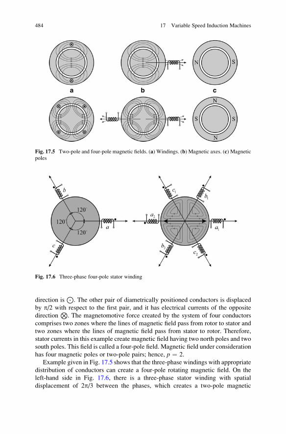
direction isJ
. The other pair of diametrically positioned conductors is displaced
by p/2 with respect to the first pair, and it has electrical currents of the opposite
directionN
. The magnetomotive force created by the system of four conductors
comprises two zones where the lines of magnetic field pass from rotor to stator and
two zones where the lines of magnetic field pass from stator to rotor. Therefore,
stator currents in this example create magnetic field having two north poles and two
south poles. This field is called a four-pole field. Magnetic field under consideration
has four magnetic poles or two-pole pairs; hence, p ¼ 2.
Example given in Fig. 17.5 shows that the three-phase windings with appropriate
distribution of conductors can create a four-pole rotating magnetic field. On the
left-hand side in Fig. 17.6, there is a three-phase stator winding with spatial
displacement of 2p/3 between the phases, which creates a two-pole magnetic
Fig. 17.5 Two-pole and four-pole magnetic fields. (a) Windings. (b) Magnetic axes. (c) Magnetic
poles
Fig. 17.6 Three-phase four-pole stator winding
484 17 Variable Speed Induction Machines
field in the air gap. A stator winding which creates a two-pole field is often called
two-pole winding. The right-hand side of the same figure shows the method of
forming a three-phase stator winding with magnetomotive force that creates a four-
pole magnetic field in the air gap. Each of the phases a, b, and c is split into two
sections, each with the same number of turns. The sections of the phase windings
are spatially displaced by p, while the angle between the neighboring sections is
p/3, which is one half of the spatial shift of a two-pole winding.
Phase a of the four-pole stator winding consists of two diametrically positioned
sections. The sections are connected in series; thus, the conductors of both sections
carry the same current ia(t). The reference terminals of each of the sections are
marked by dots. Convention of marking the reference terminal is the following:
when the current enters the dot-marked terminal of the considered section, then the
section creates the magnetomotive force and field which start from the rotor
magnetic circuit and propagate through the air gap toward the considered section.
In the case when the two sections, actually the two halves a1 and a2 of the phase
winding a, are connected in series and in such way that the phase current ia(t)enters the dot-marked terminals of both halves, magnetic field is created with two
north and two south poles. Namely, at positions y ¼ 0 and y ¼ p, it creates thefield with lines that pass from the rotor to the stator. Due to flux conservation law
(div B ¼ 0), corresponding field lines must pass from the stator to the rotor at
positions y ¼ p/2 and y ¼ 3p/2. In this way, a four-pole field is created, the field
with two pairs of poles (p ¼ 2), having two north magnetic poles and two south
magnetic poles. With phase currents ia(t), ib(t), and ic(t) that have sinusoidal
change of the same amplitude and frequency, and which are phase shifted by
2p/3, consequential magnetic field revolves at the speed determined by the supply
frequency, and it does not change the amplitude. It can be shown that the speed of
rotation Oe of the four-pole field is equal to one half of the supply frequency oe.
From Fig. 17.6, it should be noted that one of the magnetic poles is against the
section a1 at t ¼ 0, when the phase current ia(t) ¼ Im cos oet has the value
ia(t) ¼ +Im. Corresponding magnetic pole is marked by an arrow ! which is
directed toward the section a1. The phase current ib(t) ¼ Im cos(oet�2p/3) is
delayed, and it reached its maximum positive value at t1 ¼ 2p/(3oe). Over the
interval 0 < t < t1, the considered magnetic pole is shifting from the section a1toward the section b1, where it arrives at the instant t1. At t2 ¼ 4p/(3oe), the phase
current ic(t) reaches its maximum value. Then the considered magnetic pole is
placed against the section c1. At the end of one full period, at t3 ¼ 2p/oe, the
maximum of ia(t) ¼ +Im is repeated in the phase current ia(t). At the same time,
the magnetic pole being tracked reaches position against the section a2. During oneperiod of voltages and currents (electrical period) T ¼ 2p/oe, the phase change of
electrical currents is Dye ¼ 2p, while the spatial displacement of the magnetic pole
is Dym ¼ p. Therefore, the speed of rotation of the field is one half of the supply
frequency, Oe ¼ oe/2.
It should be noted that the four-pole field shown in Fig. 17.6 has two diametri-
cally positioned poles of the same polarity. During one period of variation of
electrical variables, both poles shift by p; hence, they switch their places.
17.4 Changing Pole Pairs 485
In general, when stator windings are arranged to make a rotating magnetic field
with 2p poles, the synchronous speed of the field rotation is Oe ¼ oe/p. The torqueof multipole induction machines is determined on the basis of expression Tem ¼Pd/Oe ¼ pPd/oe, according to (17.3).
By changing the number of magnetic poles, windings obtain a different number
of slots per phase, different winding factors such as belt factor and chord factor,
and different magnetic induction, winding resistance, leakage inductance, and
self-inductance.
17.4.1 Speed and Torque of Multipole Machines
The number of magnetic pole pairs of an electrical machine is denoted by p.Synchronous speed of an induction motor is equal to
Oe ¼ oe
p; (17.1)
while the speed of rotor rotation is equal to
Om ¼ om
p¼ oe � oslip
p¼ Oe � Oslip; (17.2)
where oslip is the angular frequency of the rotor currents. The electromagnetic
torque is
Tem ¼ Pd
Oe¼ p
Pd
oe: (17.3)
17.5 Characteristics of Multipole Machines
Multipole machines (p > 1) make better use of the copper and iron compared to two-
polemachines. There are applications of inductionmachineswhere selection of higher
number of poles offers higher specific torque and power compared to the solutions
involving two-pole machines. A rationale of these statements is presented here.
It is known that one turn of the phase winding of two-pole machine is positioned
diametrically at angular distance Dy� p. When one of these conductors is under the
north magnetic pole of the revolving field, the other is below the south pole. At the
front and rear of the machine, the two conductors are connected by end turns. In
two-pole machines, end turns are relatively long. Their length is one half of the
machine circumference. Longer conductors contribute to increased consumption of
486 17 Variable Speed Induction Machines
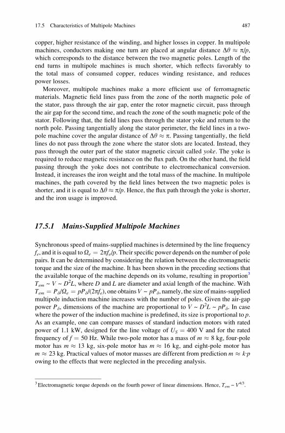
copper, higher resistance of the winding, and higher losses in copper. In multipole
machines, conductors making one turn are placed at angular distance Dy � p/p,which corresponds to the distance between the two magnetic poles. Length of the
end turns in multipole machines is much shorter, which reflects favorably to
the total mass of consumed copper, reduces winding resistance, and reduces
power losses.
Moreover, multipole machines make a more efficient use of ferromagnetic
materials. Magnetic field lines pass from the zone of the north magnetic pole of
the stator, pass through the air gap, enter the rotor magnetic circuit, pass through
the air gap for the second time, and reach the zone of the south magnetic pole of the
stator. Following that, the field lines pass through the stator yoke and return to the
north pole. Passing tangentially along the stator perimeter, the field lines in a two-
pole machine cover the angular distance of Dy � p. Passing tangentially, the field
lines do not pass through the zone where the stator slots are located. Instead, they
pass through the outer part of the stator magnetic circuit called yoke. The yoke is
required to reduce magnetic resistance on the flux path. On the other hand, the field
passing through the yoke does not contribute to electromechanical conversion.
Instead, it increases the iron weight and the total mass of the machine. In multipole
machines, the path covered by the field lines between the two magnetic poles is
shorter, and it is equal to Dy� p/p. Hence, the flux path through the yoke is shorter,and the iron usage is improved.
17.5.1 Mains-Supplied Multipole Machines
Synchronous speed of mains-supplied machines is determined by the line frequency
fe, and it is equal toOe ¼ 2pfe/p. Their specific power depends on the number of pole
pairs. It can be determined by considering the relation between the electromagnetic
torque and the size of the machine. It has been shown in the preceding sections that
the available torque of the machine depends on its volume, resulting in proportion3
Tem ~ V ~ D2L, where D and L are diameter and axial length of the machine. With
Tem ¼ Pd/Oe ¼ pPd/(2pfe), one obtainsV ~ pPd, namely, the size ofmains-supplied
multipole induction machine increases with the number of poles. Given the air-gap
power Pd, dimensions of the machine are proportional to V ~ D2L ~ pPd. In case
where the power of the induction machine is predefined, its size is proportional to p.As an example, one can compare masses of standard induction motors with rated
power of 1.1 kW, designed for the line voltage of US ¼ 400 V and for the rated
frequency of f ¼ 50 Hz. While two-pole motor has a mass of m � 8 kg, four-pole
motor has m � 13 kg, six-pole motor has m � 16 kg, and eight-pole motor has
m � 23 kg. Practical values of motor masses are different from prediction m � k∙powing to the effects that were neglected in the preceding analysis.
3 Electromagnetic torque depends on the fourth power of linear dimensions. Hence, Tem ~ V4/3.
17.5 Characteristics of Multipole Machines 487
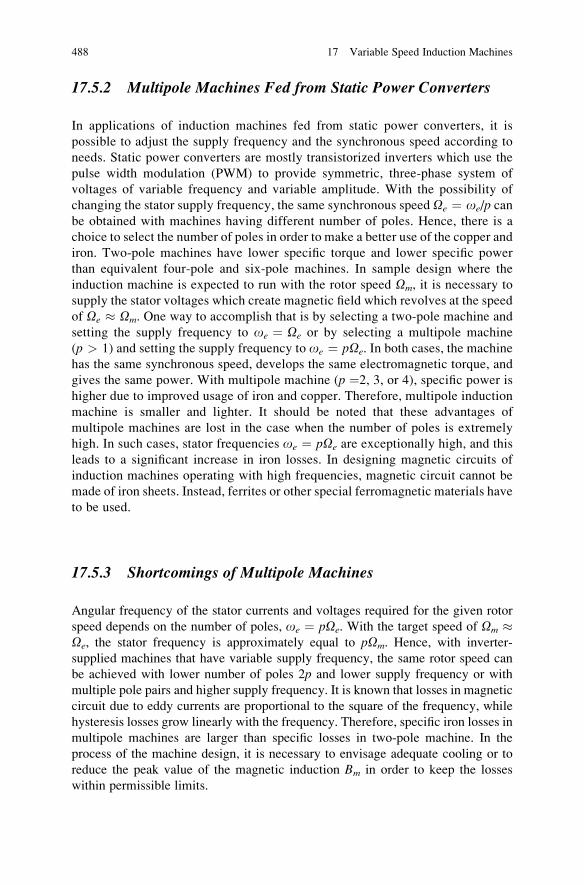
17.5.2 Multipole Machines Fed from Static Power Converters
In applications of induction machines fed from static power converters, it is
possible to adjust the supply frequency and the synchronous speed according to
needs. Static power converters are mostly transistorized inverters which use the
pulse width modulation (PWM) to provide symmetric, three-phase system of
voltages of variable frequency and variable amplitude. With the possibility of
changing the stator supply frequency, the same synchronous speed Oe ¼ oe/p canbe obtained with machines having different number of poles. Hence, there is a
choice to select the number of poles in order to make a better use of the copper and
iron. Two-pole machines have lower specific torque and lower specific power
than equivalent four-pole and six-pole machines. In sample design where the
induction machine is expected to run with the rotor speed Om, it is necessary to
supply the stator voltages which create magnetic field which revolves at the speed
of Oe � Om. One way to accomplish that is by selecting a two-pole machine and
setting the supply frequency to oe ¼ Oe or by selecting a multipole machine
(p > 1) and setting the supply frequency to oe ¼ pOe. In both cases, the machine
has the same synchronous speed, develops the same electromagnetic torque, and
gives the same power. With multipole machine (p ¼2, 3, or 4), specific power is
higher due to improved usage of iron and copper. Therefore, multipole induction
machine is smaller and lighter. It should be noted that these advantages of
multipole machines are lost in the case when the number of poles is extremely
high. In such cases, stator frequencies oe ¼ pOe are exceptionally high, and this
leads to a significant increase in iron losses. In designing magnetic circuits of
induction machines operating with high frequencies, magnetic circuit cannot be
made of iron sheets. Instead, ferrites or other special ferromagnetic materials have
to be used.
17.5.3 Shortcomings of Multipole Machines
Angular frequency of the stator currents and voltages required for the given rotor
speed depends on the number of poles, oe ¼ pOe. With the target speed of Om �Oe, the stator frequency is approximately equal to pOm. Hence, with inverter-
supplied machines that have variable supply frequency, the same rotor speed can
be achieved with lower number of poles 2p and lower supply frequency or with
multiple pole pairs and higher supply frequency. It is known that losses in magnetic
circuit due to eddy currents are proportional to the square of the frequency, while
hysteresis losses grow linearly with the frequency. Therefore, specific iron losses in
multipole machines are larger than specific losses in two-pole machine. In the
process of the machine design, it is necessary to envisage adequate cooling or to
reduce the peak value of the magnetic induction Bm in order to keep the losses
within permissible limits.
488 17 Variable Speed Induction Machines
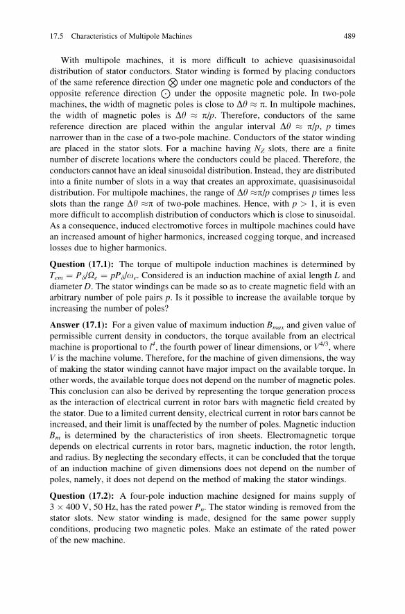
With multipole machines, it is more difficult to achieve quasisinusoidal
distribution of stator conductors. Stator winding is formed by placing conductors
of the same reference directionN
under one magnetic pole and conductors of the
opposite reference directionJ
under the opposite magnetic pole. In two-pole
machines, the width of magnetic poles is close to Dy � p. In multipole machines,
the width of magnetic poles is Dy � p/p. Therefore, conductors of the same
reference direction are placed within the angular interval Dy � p/p, p times
narrower than in the case of a two-pole machine. Conductors of the stator winding
are placed in the stator slots. For a machine having NZ slots, there are a finite
number of discrete locations where the conductors could be placed. Therefore, the
conductors cannot have an ideal sinusoidal distribution. Instead, they are distributed
into a finite number of slots in a way that creates an approximate, quasisinusoidal
distribution. For multipole machines, the range of Dy �p/p comprises p times less
slots than the range Dy �p of two-pole machines. Hence, with p > 1, it is even
more difficult to accomplish distribution of conductors which is close to sinusoidal.
As a consequence, induced electromotive forces in multipole machines could have
an increased amount of higher harmonics, increased cogging torque, and increased
losses due to higher harmonics.
Question (17.1): The torque of multipole induction machines is determined by
Tem ¼ Pd/Oe ¼ pPd/oe. Considered is an induction machine of axial length L and
diameter D. The stator windings can be made so as to create magnetic field with an
arbitrary number of pole pairs p. Is it possible to increase the available torque by
increasing the number of poles?
Answer (17.1): For a given value of maximum induction Bmax and given value of
permissible current density in conductors, the torque available from an electrical
machine is proportional to l4, the fourth power of linear dimensions, or V4/3, where
V is the machine volume. Therefore, for the machine of given dimensions, the way
of making the stator winding cannot have major impact on the available torque. In
other words, the available torque does not depend on the number of magnetic poles.
This conclusion can also be derived by representing the torque generation process
as the interaction of electrical current in rotor bars with magnetic field created by
the stator. Due to a limited current density, electrical current in rotor bars cannot be
increased, and their limit is unaffected by the number of poles. Magnetic induction
Bm is determined by the characteristics of iron sheets. Electromagnetic torque
depends on electrical currents in rotor bars, magnetic induction, the rotor length,
and radius. By neglecting the secondary effects, it can be concluded that the torque
of an induction machine of given dimensions does not depend on the number of
poles, namely, it does not depend on the method of making the stator windings.
Question (17.2): A four-pole induction machine designed for mains supply of
3 � 400 V, 50 Hz, has the rated power Pn. The stator winding is removed from the
stator slots. New stator winding is made, designed for the same power supply
conditions, producing two magnetic poles. Make an estimate of the rated power
of the new machine.
17.5 Characteristics of Multipole Machines 489
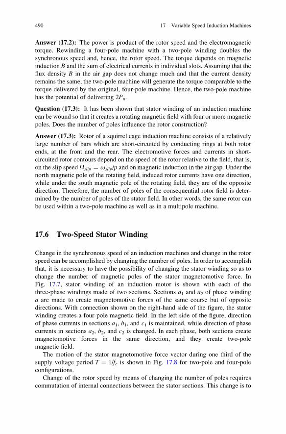
Answer (17.2): The power is product of the rotor speed and the electromagnetic
torque. Rewinding a four-pole machine with a two-pole winding doubles the
synchronous speed and, hence, the rotor speed. The torque depends on magnetic
induction B and the sum of electrical currents in individual slots. Assuming that the
flux density B in the air gap does not change much and that the current density
remains the same, the two-pole machine will generate the torque comparable to the
torque delivered by the original, four-pole machine. Hence, the two-pole machine
has the potential of delivering 2Pn.
Question (17.3): It has been shown that stator winding of an induction machine
can be wound so that it creates a rotating magnetic field with four or more magnetic
poles. Does the number of poles influence the rotor construction?
Answer (17.3): Rotor of a squirrel cage induction machine consists of a relatively
large number of bars which are short-circuited by conducting rings at both rotor
ends, at the front and the rear. The electromotive forces and currents in short-
circuited rotor contours depend on the speed of the rotor relative to the field, that is,
on the slip speed Oslip ¼ oslip/p and on magnetic induction in the air gap. Under the
north magnetic pole of the rotating field, induced rotor currents have one direction,
while under the south magnetic pole of the rotating field, they are of the opposite
direction. Therefore, the number of poles of the consequential rotor field is deter-
mined by the number of poles of the stator field. In other words, the same rotor can
be used within a two-pole machine as well as in a multipole machine.
17.6 Two-Speed Stator Winding
Change in the synchronous speed of an induction machines and change in the rotor
speed can be accomplished by changing the number of poles. In order to accomplish
that, it is necessary to have the possibility of changing the stator winding so as to
change the number of magnetic poles of the stator magnetomotive force. In
Fig. 17.7, stator winding of an induction motor is shown with each of the
three-phase windings made of two sections. Sections a1 and a2 of phase winding
a are made to create magnetomotive forces of the same course but of opposite
directions. With connection shown on the right-hand side of the figure, the stator
winding creates a four-pole magnetic field. In the left side of the figure, direction
of phase currents in sections a1, b1, and c1 is maintained, while direction of phase
currents in sections a2, b2, and c2 is changed. In each phase, both sections create
magnetomotive forces in the same direction, and they create two-pole
magnetic field.
The motion of the stator magnetomotive force vector during one third of the
supply voltage period T ¼ 1/fe is shown in Fig. 17.8 for two-pole and four-pole
configurations.
Change of the rotor speed by means of changing the number of poles requires
commutation of internal connections between the stator sections. This change is to
490 17 Variable Speed Induction Machines
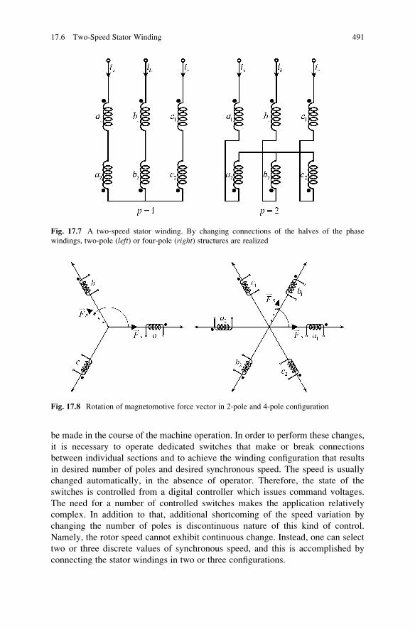
be made in the course of the machine operation. In order to perform these changes,
it is necessary to operate dedicated switches that make or break connections
between individual sections and to achieve the winding configuration that results
in desired number of poles and desired synchronous speed. The speed is usually
changed automatically, in the absence of operator. Therefore, the state of the
switches is controlled from a digital controller which issues command voltages.
The need for a number of controlled switches makes the application relatively
complex. In addition to that, additional shortcoming of the speed variation by
changing the number of poles is discontinuous nature of this kind of control.
Namely, the rotor speed cannot exhibit continuous change. Instead, one can select
two or three discrete values of synchronous speed, and this is accomplished by
connecting the stator windings in two or three configurations.
Fig. 17.8 Rotation of magnetomotive force vector in 2-pole and 4-pole configuration
Fig. 17.7 A two-speed stator winding. By changing connections of the halves of the phase
windings, two-pole (left) or four-pole (right) structures are realized
17.6 Two-Speed Stator Winding 491
The appearance of transistorized inverters that operated on pulse width modula-
tion principles opens the possibility for continuous change of the supply frequency,
thus eliminating the need for changing the number of poles.
Question (17.4): A two-pole induction machine designed for mains supply
develops the breakdown torque at the speed of nb ¼ 2,000 rpm. The stator winding
is removed and a four-pole winding is built instead. Determine the speed where the
four-pole machine develops the breakdown torque.
Answer (17.4): Electromagnetic torque is equal to the ratio of the air-gap power
and synchronous speed. The air-gap power is the highest at the relative slip sb ¼RR/(Lgeoe), that is, at the rotor frequency ofob ¼ RR/Lge. Therefore, the breakdowntorque is developed at the rotor frequency that does not depend on the number of
poles. Relative value of the breakdown slip is equal to sb ¼ (ne�nb)/ne ¼ 1/3. For
the two-pole machine, nb ¼ 2,000 rpm, while for the four-pole machine, the speed
that results in the breakdown torque is nb ¼ ne(1�sb) ¼ 1,500(1�sb) ¼ 1,000 rpm.
17.7 Notation
Preceding considerations use the lower case letter o for denoting angular frequency
of electrical currents and voltages. Mechanical speeds of the rotor, speed of
revolving magnetic field and magnetomotive force, and other mechanical quantities
are denoted by the upper case letter O. A survey of notation using the sample
multipole machine is presented below. In the case of two-pole machines, where
p ¼ 1, all electrical quantities o are equal to mechanical quantities O. Unlessotherwise stated, all the quantities are expressed in rad/s:
• Oe – synchronous speed, angular speed of rotation of the magnetic field
• oe ¼ pOe – angular frequency of power supply, frequency of the stator currents
and voltages
• Om – the rotor speed
• om ¼ pOm – electrical representation of the rotor speed
• n ¼ 9.54Om – the rotor speed expressed in rpm (revolutions per minute)
• oslip ¼ oe�pOm – angular frequency of the rotor currents
• Oslip ¼ Oe�Om – the slip speed of the rotor, the speed of lagging behind the
synchronous speed
For a four-pole inductionmachine (p ¼ 2) with rated supply frequency fe ¼ 50Hz
and rated speed of nn ¼ 1,350 rpm, characteristic angular frequencies and speeds in
rated operating conditions are the following:
– Angular frequency of stator voltages – oe ¼ 100p– Synchronous speed – Oe ¼ 50p, ne ¼ 1,500 rpm
– Angular frequency of rotor currents – oslip ¼ 10p– Slip speed – Oslip ¼ 5p, nslip ¼ 150 rpm
– Rotor mechanical speed – Om ¼ 45p, nn ¼ 1,350 rpm
492 17 Variable Speed Induction Machines
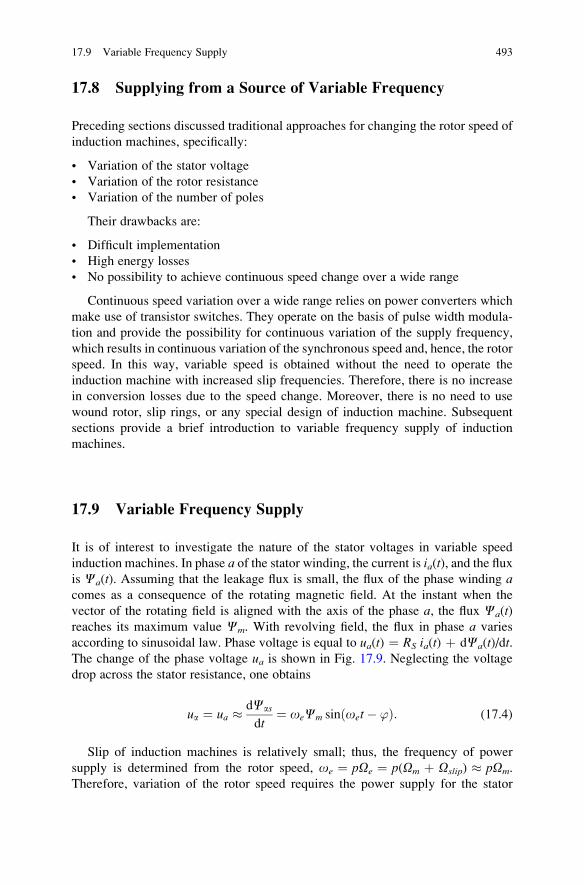
17.8 Supplying from a Source of Variable Frequency
Preceding sections discussed traditional approaches for changing the rotor speed of
induction machines, specifically:
• Variation of the stator voltage
• Variation of the rotor resistance
• Variation of the number of poles
Their drawbacks are:
• Difficult implementation
• High energy losses
• No possibility to achieve continuous speed change over a wide range
Continuous speed variation over a wide range relies on power converters which
make use of transistor switches. They operate on the basis of pulse width modula-
tion and provide the possibility for continuous variation of the supply frequency,
which results in continuous variation of the synchronous speed and, hence, the rotor
speed. In this way, variable speed is obtained without the need to operate the
induction machine with increased slip frequencies. Therefore, there is no increase
in conversion losses due to the speed change. Moreover, there is no need to use
wound rotor, slip rings, or any special design of induction machine. Subsequent
sections provide a brief introduction to variable frequency supply of induction
machines.
17.9 Variable Frequency Supply
It is of interest to investigate the nature of the stator voltages in variable speed
induction machines. In phase a of the stator winding, the current is ia(t), and the fluxis Ca(t). Assuming that the leakage flux is small, the flux of the phase winding acomes as a consequence of the rotating magnetic field. At the instant when the
vector of the rotating field is aligned with the axis of the phase a, the flux Ca(t)reaches its maximum value Cm. With revolving field, the flux in phase a varies
according to sinusoidal law. Phase voltage is equal to ua(t) ¼ RS ia(t) þ dCa(t)/dt.The change of the phase voltage ua is shown in Fig. 17.9. Neglecting the voltage
drop across the stator resistance, one obtains
ua ¼ ua � dCas
dt¼ oeCm sinðoet� ’Þ: (17.4)
Slip of induction machines is relatively small; thus, the frequency of power
supply is determined from the rotor speed, oe ¼ pOe ¼ p(Om þ Oslip) � pOm.
Therefore, variation of the rotor speed requires the power supply for the stator
17.9 Variable Frequency Supply 493
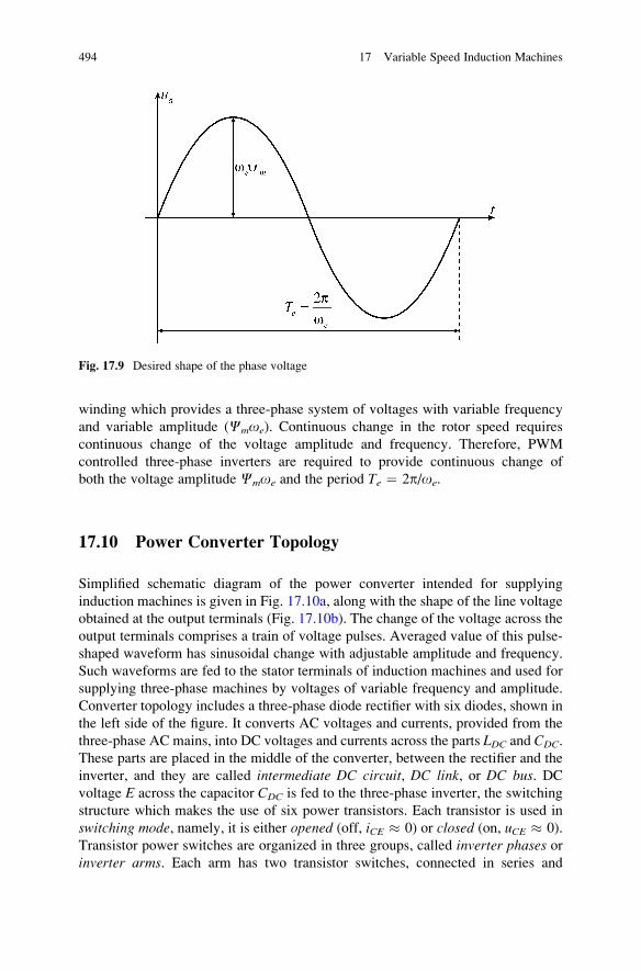
winding which provides a three-phase system of voltages with variable frequency
and variable amplitude (Cmoe). Continuous change in the rotor speed requires
continuous change of the voltage amplitude and frequency. Therefore, PWM
controlled three-phase inverters are required to provide continuous change of
both the voltage amplitude Cmoe and the period Te ¼ 2p/oe.
17.10 Power Converter Topology
Simplified schematic diagram of the power converter intended for supplying
induction machines is given in Fig. 17.10a, along with the shape of the line voltage
obtained at the output terminals (Fig. 17.10b). The change of the voltage across the
output terminals comprises a train of voltage pulses. Averaged value of this pulse-
shaped waveform has sinusoidal change with adjustable amplitude and frequency.
Such waveforms are fed to the stator terminals of induction machines and used for
supplying three-phase machines by voltages of variable frequency and amplitude.
Converter topology includes a three-phase diode rectifier with six diodes, shown in
the left side of the figure. It converts AC voltages and currents, provided from the
three-phase AC mains, into DC voltages and currents across the parts LDC and CDC.
These parts are placed in the middle of the converter, between the rectifier and the
inverter, and they are called intermediate DC circuit, DC link, or DC bus. DCvoltage E across the capacitor CDC is fed to the three-phase inverter, the switching
structure which makes the use of six power transistors. Each transistor is used in
switching mode, namely, it is either opened (off, iCE � 0) or closed (on, uCE � 0).
Transistor power switches are organized in three groups, called inverter phases orinverter arms. Each arm has two transistor switches, connected in series and
Fig. 17.9 Desired shape of the phase voltage
494 17 Variable Speed Induction Machines
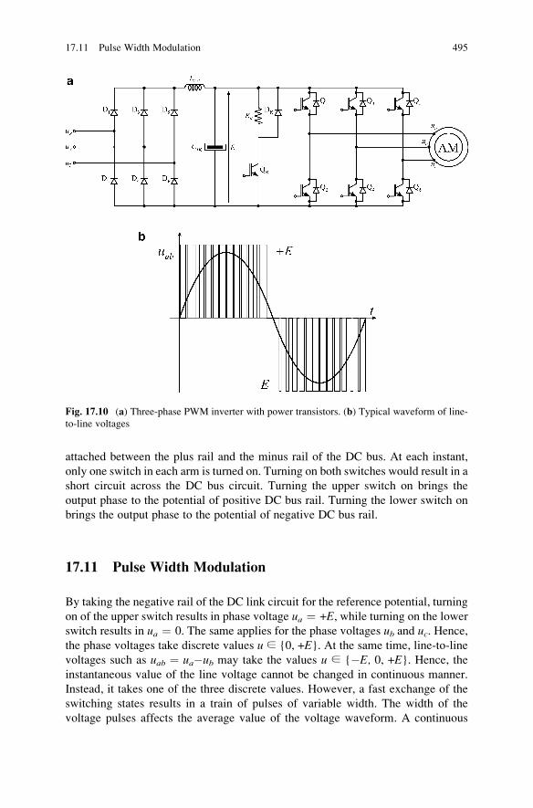
attached between the plus rail and the minus rail of the DC bus. At each instant,
only one switch in each arm is turned on. Turning on both switches would result in a
short circuit across the DC bus circuit. Turning the upper switch on brings the
output phase to the potential of positive DC bus rail. Turning the lower switch on
brings the output phase to the potential of negative DC bus rail.
17.11 Pulse Width Modulation
By taking the negative rail of the DC link circuit for the reference potential, turning
on of the upper switch results in phase voltage ua ¼ +E, while turning on the lowerswitch results in ua ¼ 0. The same applies for the phase voltages ub and uc. Hence,the phase voltages take discrete values u ∈ {0, +E}. At the same time, line-to-line
voltages such as uab ¼ ua�ub may take the values u ∈ {�E, 0, +E}. Hence, theinstantaneous value of the line voltage cannot be changed in continuous manner.
Instead, it takes one of the three discrete values. However, a fast exchange of the
switching states results in a train of pulses of variable width. The width of the
voltage pulses affects the average value of the voltage waveform. A continuous
Fig. 17.10 (a) Three-phase PWM inverter with power transistors. (b) Typical waveform of line-
to-line voltages
17.11 Pulse Width Modulation 495
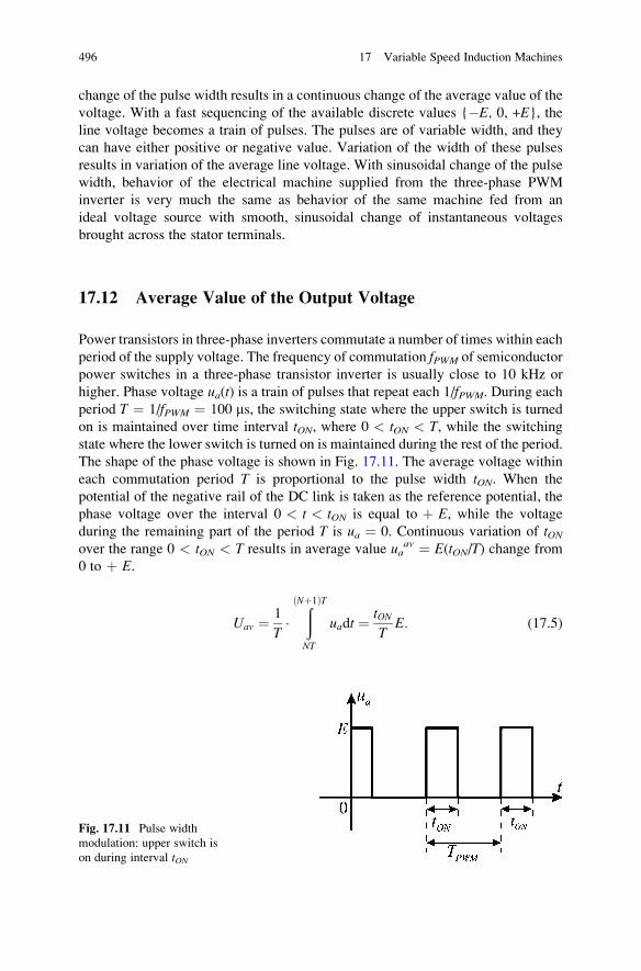
change of the pulse width results in a continuous change of the average value of the
voltage. With a fast sequencing of the available discrete values {�E, 0, +E}, theline voltage becomes a train of pulses. The pulses are of variable width, and they
can have either positive or negative value. Variation of the width of these pulses
results in variation of the average line voltage. With sinusoidal change of the pulse
width, behavior of the electrical machine supplied from the three-phase PWM
inverter is very much the same as behavior of the same machine fed from an
ideal voltage source with smooth, sinusoidal change of instantaneous voltages
brought across the stator terminals.
17.12 Average Value of the Output Voltage
Power transistors in three-phase inverters commutate a number of times within each
period of the supply voltage. The frequency of commutation fPWM of semiconductor
power switches in a three-phase transistor inverter is usually close to 10 kHz or
higher. Phase voltage ua(t) is a train of pulses that repeat each 1/fPWM. During each
period T ¼ 1/fPWM ¼ 100 ms, the switching state where the upper switch is turned
on is maintained over time interval tON, where 0 < tON < T, while the switching
state where the lower switch is turned on is maintained during the rest of the period.
The shape of the phase voltage is shown in Fig. 17.11. The average voltage within
each commutation period T is proportional to the pulse width tON. When the
potential of the negative rail of the DC link is taken as the reference potential, the
phase voltage over the interval 0 < t < tON is equal to þ E, while the voltage
during the remaining part of the period T is ua ¼ 0. Continuous variation of tONover the range 0 < tON < T results in average value ua
av ¼ E(tON/T) change from0 to þ E.
Uav ¼ 1
T�
ððNþ1ÞT
NT
uadt ¼ tONT
E: (17.5)
Fig. 17.11 Pulse width
modulation: upper switch is
on during interval tON
496 17 Variable Speed Induction Machines
17.13 Sinusoidal Output Voltages
The width of the voltage pulses that constitute the phase voltage can be varied or
modulated. Variation of the pulse width is called pulse width modulation (PWM).
Starting from the expression uaav ¼ E(tON/T), desired average voltage ua
av can be
used to calculate the time tON, which determines the average value of the phase
voltage within one switching period T ¼ 1/fPWM.
In order to achieve variation of the average voltage value uaav(t), that is, to obtain
the phase voltage that changes the average value in successive switching periods T,the pulse width tON should change as tON(t) ¼ T ua
av(t)/Е. As a matter of fact, it is not
correct towrite tON(t), as the pulsewidth assumes one discrete value in each switching
period T. Namely, the pulse width over the period [nT..(n þ 1)T] is determined by
discrete value tON(n) ¼ T uaav(n)/Е. If fe ¼ 50 Hz is the desired frequency of
the phase voltage, while’ is the initial phase, and the number 0 < A < 1 determines
the desired amplitude, the pulse width should be varied according to
tONðnÞ ¼ T
2þ T
2A sinð2pfe � nT � ’Þ: (17.6)
With this change of the pulse width, the phase voltage ua is obtained with
average value over successive intervals T that change according to expression
uava ðnÞ �E
2þ E
2A sinð2pfe � nT � ’Þ: (17.7)
The frequency component fe of the phase voltage has the amplitude which can be
varied by changing parameter A, while the frequency and phase are determined by
parameters fe and ’. Commutation frequency fPWM has to be considerably higher
than the desired frequency of the phase voltage, fe < < fPWM. In the expression for
uaav(n), there is a DC component of the voltage which is equal to E/2. This is the
consequence of selecting the negative rail of the DC bus for the reference potential
V0. By turning on the upper switchQ1 in Fig. 17.10a, the phase voltage ua is equal toE. With Q2 turned on, ua ¼ 0. Other choices for reference potential result in
different values of the phase voltage ua.DC component in the phase voltages is equal in all three phases. It has no impact
on the operation of the induction machine. Namely, the stator winding is connected
to three-phase inverter by three conductors, and the operation of the machine is
determined by line-to-line voltages. Line-to-line voltage uab is equal to ua-ub.Subtracting the two-phase voltages removes the DC components. It is of interest
to point out that the choice of the reference potential is arbitrary one. Therefore, it
cannot have an impact on the operation of the electrical machine. In order to
confirm this statement, one can calculate the line voltage uabav(t) as the difference
between the phase voltages uaav(t) and ub
av(t). The voltage uaav(t) is given in (17.7)
while the voltage ubav(t) is equal to
17.13 Sinusoidal Output Voltages 497
uavb ðtÞ �E
2þ E
2A sinð2pfe � nT � ’� 2p=3Þ;
and it lags behind ua by 2p/3. By calculating uabav(t) ¼ ua
av(t) – ubav(t), DC
components E/2 are canceled, resulting in line-to-line voltage uabav which does
not have a DC component:
uavabðtÞ �AE
ffiffiffi3
p
2sinð2pfe � nT � ’þ p=6Þ:
Digital implementation of the pulse width modulation implies that parameters A,fe, and ’ are the numbers represented by binary record in RAM memory. They can
be adjusted to the needs of the actual operating regime of the induction machine.
Within each period Te ¼ 1/fe of phase voltages, there are a finite number of
pulses. The width of these pulses is modulated (changed) in the way to obtain
sinusoidal change of the average value uav(t).The process of approximating sinusoidal change of the phase voltage by means
of a finite train of pulse width-modulated impulses has similarities with the proce-
dure of making distributed windings with quasisinusoidal distribution of conductors
placed in a finite number of slots.
17.14 Spectrum of PWM Waveforms
Sinusoidal PWM is used to obtain a sequence of variable width pulses. Averaged
pulses provide the phase voltages of the desired frequency fe. When the pulse width
has sinusoidal change, according to expression tON(n) ¼ (T/2) [1þ Asin(2pfe nT�’)],the average values with each switching period T ¼ 1/fPWM change according to
expression uav(n)�(E/2) þ (E/2) A sin(2pfe nT�’).The commutation frequency fPWM has to be considerably higher than the desired
frequency of the phase voltage, fe << fPWM, so as to obtain a smooth, gradual
change of average voltage between the successive switching periods T ¼ 1/fPWM
and to obtain the operation similar to feeding the machine from an ideal source. The
frequency fe of the phase voltages determines the synchronous speed, and it is called
basic or fundamental. It ranges from several tens to several hundreds of cycles per
second. The frequency fPWM is called commutation or switching frequency, and it
ranges from 5 to 20 kHz.
The spectrum of a pulse width-modulated sequence of phase voltage pulses
contains:
• DC component E/2• Slowly varying AC component of frequency fe, created by sinusoidal variation of
the pulse width, called the basic or fundamental frequency component
498 17 Variable Speed Induction Machines
• Frequency component at the commutation frequency fPWM ¼ 1/T, created by thetrain of variable width voltage pulses that keep repeating each T
• A series of frequency components with smaller amplitudes and with frequencies
m∙fPWM that are integer multiples of the switching frequency fPWM
• A series of frequency components at frequencies m∙fPWM � n∙fe, produced by
interaction between the switching frequency fPWM and the basic frequency fe
DC component of the phase voltage is the same in all phases; thus, it has no
influence on line voltages. The fundamental AC component at the basic frequency
fe is the desired result, the voltage required across the stator terminals. It has
adjustable amplitude and adjustable frequency. Assuming that the high-frequency
content of the spectrum can be neglected, the three-phase inverter with PWM
control can be regarded as the source of sinusoidal voltages with adjustable
amplitude and adjustable fundamental frequency fe.Spectral component at the switching frequency fPWM ¼ 1/T � 10 kHz is the
consequence of the pulsating nature of the three-phase inverter. Component of the
voltage at the switching frequency has the amplitude determined by the DC link
voltage E. Due to considerable amplitude, the effects of this frequency component
cannot be neglected. The effects of the pulsed supply on an induction machine
should be analyzed in order to establish the impact of pulsating voltage on the
machine and verify whether this way of supplying the stator winding is acceptable.
Subsequent discussion proves that the stator current, the electromagnetic torque,
and the rotor speed of an induction machine, supplied from PWM controlled three-
phase inverter, resemble the current, torque, and speed obtained with an equivalent
source of smooth, sinusoidal phase voltages. Therefore, the operation with PWM
power supply can be considered equivalent to the operation with an ideal source of
sinusoidal waveforms providing the voltages of instantaneous value such as
u(t) ¼ (E/2) þ (E/2)∙Asin(2pfet – ’).
17.15 Current Ripple
The voltage balance in the phase winding a is given by the equation ua(t) ¼ RSia(t)þ dCa/dt. The flux Ca can be represented as sum of the mutual flux Cma, which
passes through the air gap and encircles both stator and rotor windings, and the
leakage flux of the stator winding, which is proportional to the leakage inductance
Lg. The voltage balance equation assumes the form ua(t) ¼ RSia(t) þ Lgdia(t)/dt þdCma/dt, where Lgia(t) is the leakage flux in the phase a of the stator winding.
Rotating magnetic field changes its relative position with respect to the phase
winding a; thus, the flux Cma exhibits sinusoidal change of the frequency deter-
mined by the synchronous speed. For this reason, the electromotive force dCma/dt issinusoidal, and it has the frequency oe � om and the amplitude Cmoe, where Cm
represents the maximum value of the mutual flux. With fe <<fPWM, the change in
the considered electromotive force is slow compared to the switching phenomena.
17.15 Current Ripple 499
While considering the effects of switching power supply on the machine behavior,
slow variations of the electromotive force can be neglected; thus, the voltage
balance equation reduces to ua(t) ¼ RSia(t) þ Lgdia(t)/dt.By applying Laplace transform on previous differential equation, one obtains
complex image of the stator current, Ia(s) ¼ Ua(s)/(RS þ sLg). Function W(s) ¼1/(RS þ sLg) represents transfer function of the stator winding, which is the ratio ofthe complex image of the stator current and the complex image of the stator voltage.
Transfer functionW(s) provides the means to calculate the stator current response to
excitation by the stator voltage of known amplitude and frequency. In the case of
interest, the voltage excitation has the switching frequency fPWM. The function is
obtained by neglecting slow-varying electromotive force; thus, it is applicable for
calculating the response at frequencies as high as fPWM, but it cannot be used for the
analysis of the machine response to lower excitation frequencies, such as the
fundamental frequency fe.The ratio of the current and voltage at the frequency o ¼ 2p/T ¼ 2pfPWM is
obtained by introducing s ¼ jo in function W(s); thus, the function assumes the
formW(jo) ¼ 1/(RS þ joLg). At switching frequencies of the order of several kHz,it is justified to introduce the assumption RS << oLg and to obtain relation jI(-jo)/U(jo)j � 1/(Lgo). This expression shows that electrical machines behave as
low-pass filters. When exposed to high-frequency voltages, the stator current
response to such excitation is smaller as the excitation frequency increases. In
other words, low-frequency excitation has much larger impact on the stator currents
than high-frequency excitation. At frequencies close to fPWM � 10 kHz, reactance
Lgo is so large that the voltage pulses have a very small influence on the stator
currents. Typical change of the phase current of an induction machine supplied
from three-phase PWM inverter is shown in Fig. 17.12.
With pulsed supply, the phase voltages exceed the desired sinusoidal waveform
during tON and then fall below during the reminder of the PWM switching period.
Therefore, the stator currents oscillate around their mean values. These oscillations
have the frequency of the switching bridge fPWM ¼ 1/T ¼ o/(2p). When the
switching frequency is sufficiently high, the amplitude of these oscillations is rather
small, and their effect on the operation of the induction machine can be neglected.
An estimate of the amplitude of oscillations of the stator current can be obtained by
using expression jI(jo)/U(jo)j � 1/(Lgo). This expression is applicable for excita-
tion by sinusoidal voltages of the frequency o ¼ 2p fPWM. The three-phase
switching inverter does not output sinusoidal waveforms at the switching fre-
quency. Instead, it provides rectangular voltage pulses of the period 1/fPWM.
Nonetheless, the formula can be used to obtain a rough estimate of the stator current
oscillations, also called ripple. In most cases, the current ripple amounts from 1% to
5% of the rated current.
Question (17.5): Induction machine of rated frequency fen ¼ 50 Hz has an equiv-
alent leakage reactance xge ¼ 20%. The machine is supplied from a three-phase
transistor inverter of the switching frequency fPWM ¼ 10 kHz. Provide an estimate
of the stator current ripple that appears due to pulsed power supply.
500 17 Variable Speed Induction Machines
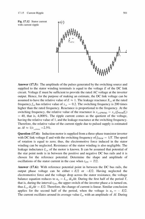
Answer (17.5): The amplitude of the pulses generated by the switching source and
supplied to the stator winding terminals is equal to the voltage E of the DC link
circuit. Voltage E must be sufficient to provide the rated AC voltage at the inverter
output. Hence, for the purpose of making an estimate, the DC link voltage can be
assumed to have the relative value of E � 1. The leakage reactance Xge at the rated
frequency fen has relative value of xge ¼ 0.2. The switching frequency is 200 times
higher than the rated frequency. Reactance is proportional to the frequency. At the
switching frequency, the relative value of the reactance is xge(PWM) ¼ xge(fPWM/fe)¼ 40, that is, 4,000%. The ripple current comes as the quotient of the voltage,
having the relative value of 1, and the leakage reactance at the switching frequency.
Therefore, the relative value of the current ripple due to pulsed supply is estimated
as DI � 1/xge(PWM)
¼2.5%.
Question (17.6): Induction motor is supplied from a three-phase transistor inverter
with DC link voltage E and with the switching frequency of fPWM ¼ 1/T. The speedof rotation is equal to zero; thus, the electromotive force induced in the stator
winding can be neglected. Resistance of the stator winding is also negligible. The
leakage inductance Lge of the motor is known. It can be assumed that potential of
the star point node is in between the positive and negative DC bus rails and it is
chosen for the reference potential. Determine the shape and amplitude of
oscillations of the stator current in the case when tON ¼ T/2.
Answer (17.6): With reference potential point in between the DC bus rails, the
output phase voltage can be either þ E/2 or �E/2. Having neglected the
electromotive force and the voltage drop across the stator resistance, the voltage
balance equation reduces to ua ¼ Lge dia/dt. During the first half of the period T,that is, during the interval tON, the upper switch of the inverter phase a is turned on,thus Lge dia/dt ¼ E/2. Therefore, the change of current is linear. Similar conclusion
applies for the second half of the period, when the voltage is ua ¼ � E/2.The current oscillates around its average value Iav with an amplitude of DI. During
Fig. 17.12 Stator current
with current ripple
17.15 Current Ripple 501
first half of the period, it increases from Iav – DI to Iav þ DI. In the second half
period, it slides back to Iav�DI. Hence, it changes by 2DI within each half period.
The change of the current is linear. Therefore, the slope dia/dt is equal to 2DI/(T/2) ¼ (E/2)/Lge. From this expression, DI ¼ ET/(8Lge).
17.16 Frequency Control
By varying the frequency of the stator winding power supply, one varies the
synchronous speed Oe of induction machine. When operating with Tem ¼ 0 and
s ¼ 0, the rotor revolves at the synchronous speed, thus Om ¼ Oe. Therefore,
continuous change of the supply frequency contributes to continuous change of
the no load speed. Considering the mechanical characteristic Tem(Om), the stator
supply frequency determines the intersection with the abscissa. For that reason, the
frequency changes would affect as well the rotor speed of loaded induction
machines. A family of mechanical characteristics obtained by varying the stator
frequency is shown in Fig. 17.13.
In addition to the no load speed, mechanical characteristic of an induction
machine is also characterized by the breakdown torque, breakdown slip, and
stiffness S ¼ jDTem/DOmj. Breakdown slip Ob ¼ pob ¼ pRR/Lge is determined by
the machine parameters, and it does not depend on the power supply frequency. The
breakdown torque Tb ¼ (3p/4)CS2/Lge and the stiffness of the mechanical charac-
teristic S ¼ kCS2/RR both depend on the square of the stator flux CS
2. The ampli-
tude of the stator flux depends on the ratio of the power supply voltage and
frequency. While operating with the rotor speeds lower than the rated speed On, it
is desirable to maintain the rated flux, that is, the maximum flux that can be
achieved within the machine. At high speeds, it is necessary to perform the field
weakening and to operate with the flux inversely proportional to the speed. With
Om > On, the flux has to be reduced in order to maintain the stator voltage US
within the limits of the rated voltage Un.
To achieve flux control, it is necessary to perform simultaneous change of the
supply voltage and the supply frequency. Relation between the voltage, frequency,
and flux is derived from the equivalent circuit. The voltage balance equation of the
stator winding of an induction machine which operates at steady state is
Us ¼ RsIs þ joeðLgsIs þCmÞ: (17.8)
By neglecting the voltage drop across the stator resistance, voltage balance
equation of the stator winding at steady state becomes US � joeCS ¼ joeLgS þjoeCm ¼ joeLgS iS þ joeLmIm. The flux amplitude is determined by the ratio of the
maximum voltage and the supply frequency, CS�US/oe. When the stator voltages
are obtained from a three-phase transistor inverter, the frequency oe of the basic
(fundamental) component determines the synchronous speed, while the quotient of
the voltage amplitude and the angular frequencyoe determines the amplitude of the
502 17 Variable Speed Induction Machines
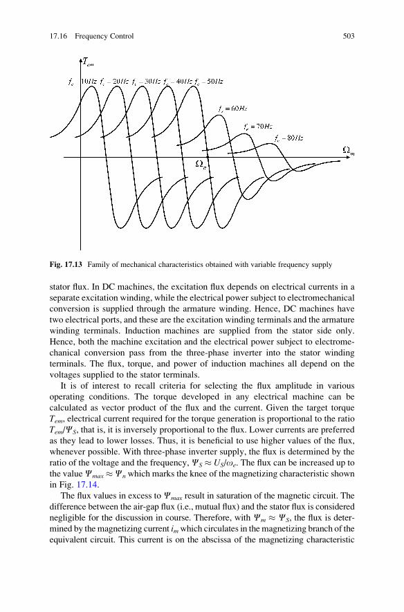
stator flux. In DC machines, the excitation flux depends on electrical currents in a
separate excitation winding, while the electrical power subject to electromechanical
conversion is supplied through the armature winding. Hence, DC machines have
two electrical ports, and these are the excitation winding terminals and the armature
winding terminals. Induction machines are supplied from the stator side only.
Hence, both the machine excitation and the electrical power subject to electrome-
chanical conversion pass from the three-phase inverter into the stator winding
terminals. The flux, torque, and power of induction machines all depend on the
voltages supplied to the stator terminals.
It is of interest to recall criteria for selecting the flux amplitude in various
operating conditions. The torque developed in any electrical machine can be
calculated as vector product of the flux and the current. Given the target torque
Tem, electrical current required for the torque generation is proportional to the ratio
Tem/CS, that is, it is inversely proportional to the flux. Lower currents are preferred
as they lead to lower losses. Thus, it is beneficial to use higher values of the flux,
whenever possible. With three-phase inverter supply, the flux is determined by the
ratio of the voltage and the frequency,CS � US/oe. The flux can be increased up to
the valueCmax �Cnwhich marks the knee of the magnetizing characteristic shown
in Fig. 17.14.
The flux values in excess toCmax result in saturation of the magnetic circuit. The
difference between the air-gap flux (i.e., mutual flux) and the stator flux is considered
negligible for the discussion in course. Therefore, with Cm � CS, the flux is deter-
mined by the magnetizing current imwhich circulates in the magnetizing branch of the
equivalent circuit. This current is on the abscissa of the magnetizing characteristic
Fig. 17.13 Family of mechanical characteristics obtained with variable frequency supply
17.16 Frequency Control 503
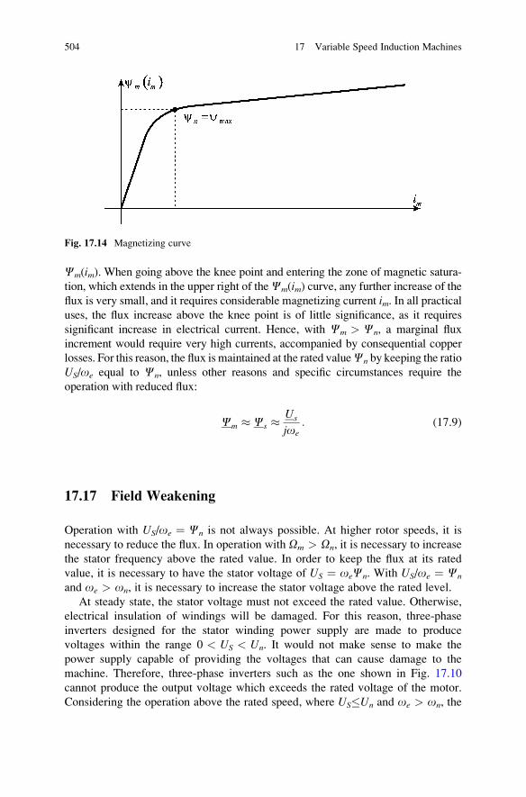
Cm(im). When going above the knee point and entering the zone of magnetic satura-
tion, which extends in the upper right of theCm(im) curve, any further increase of theflux is very small, and it requires considerable magnetizing current im. In all practicaluses, the flux increase above the knee point is of little significance, as it requires
significant increase in electrical current. Hence, with Cm > Cn, a marginal flux
increment would require very high currents, accompanied by consequential copper
losses. For this reason, the flux is maintained at the rated valueCn by keeping the ratio
US/oe equal to Cn, unless other reasons and specific circumstances require the
operation with reduced flux:
Cm � Cs �Us
joe: (17.9)
17.17 Field Weakening
Operation with US/oe ¼ Cn is not always possible. At higher rotor speeds, it is
necessary to reduce the flux. In operation with Om > On, it is necessary to increase
the stator frequency above the rated value. In order to keep the flux at its rated
value, it is necessary to have the stator voltage of US ¼ oeCn. With US/oe ¼ Cn
and oe > on, it is necessary to increase the stator voltage above the rated level.
At steady state, the stator voltage must not exceed the rated value. Otherwise,
electrical insulation of windings will be damaged. For this reason, three-phase
inverters designed for the stator winding power supply are made to produce
voltages within the range 0 < US < Un. It would not make sense to make the
power supply capable of providing the voltages that can cause damage to the
machine. Therefore, three-phase inverters such as the one shown in Fig. 17.10
cannot produce the output voltage which exceeds the rated voltage of the motor.
Considering the operation above the rated speed, where US�Un and oe > on, the
Fig. 17.14 Magnetizing curve
504 17 Variable Speed Induction Machines
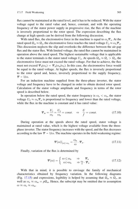
flux cannot be maintained at the rated level, and it has to be reduced. With the stator
voltage equal to the rated value and, hence, constant, and with the operating
frequency of the stator power supply in progressive rise, the flux of the machine
is inversely proportional to the rotor speed. The expression describing the flux
change at high speeds can be derived from the following discussion.
With rated flux, the electromotive force in the machine is equal to oeCn. At the
rated speed Om � On, the electromotive force reaches the rated voltage Un � onCn.
This discussion neglects the slip and overlooks the difference between the air-gap
flux and the stator flux. With limited voltage, the rated flux cannot be maintained in
operation above the rated speed. The highest sustainable voltage that is applicable
to the stator terminals is the stator rated voltage Un. At speeds Om � Oe > On, the
electromotive force must not exceed the rated voltage. For that to achieve, the flux
must not exceed CS(oe) ¼ Cn(on/oe). In this case, the electromotive force would
be equal to the rated voltage. At higher speeds, the flux is inversely proportional
to the rotor speed and, hence, inversely proportional to the supply frequency,
C ~ 1/o.For an induction machine supplied from the three-phase inverter, the stator
voltage and frequency have to be changed in order to obtain desired rotor speed.
Calculation of the stator voltage amplitude and frequency in terms of the rotor
speed is described below.
In operation below the rated speed, the stator frequency is oe < on, the stator
voltage US � oeCn is proportional to frequency and lower than the rated voltage,
while the flux in the machine is constant and it has rated value:
Cm ¼ Us
oe¼ Un
on¼ const: ) U
f¼ const: (17.10)
During operation at the speeds above the rated speed, stator voltage is
maintained at rated value, which is the highest voltage available from the three-
phase inverter. The stator frequency increases with the speed, and the flux decreases
according to the lawC ~ 1/o. The machine operates in the field weakening regime:
CðoÞj oj j>on¼ on
o�Cn: (17.11)
Finally, variation of the flux is determined by
CðoÞ ¼ o�on ) Cn
o>on ) on
o �Cn
�: (17.12)
With that in mind, it is possible to envisage the family of mechanical
characteristics obtained by frequency variation. In the following diagrams
(Fig. 17.15) and expressions, legibility is helped by assuming that Om � Oe, as
well as oe � om ¼ pOm. Hence, the subscript may be omitted due to assumption
o � oe � om.
17.17 Field Weakening 505
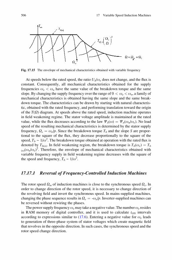
At speeds below the rated speed, the ratio US/oe does not change, and the flux is
constant. Consequently, all mechanical characteristics obtained for the supply
frequencies oe < on have the same value of the breakdown torque and the same
slope. By changing the supply frequency over the range of 0 < oe<on, a family of
mechanical characteristics is obtained having the same slope and the same break-
down torque. The characteristics can be drawn by starting with natural characteris-
tic, obtained with the rated frequency, and performing translation toward the origin
of the T(O) diagram. At speeds above the rated speed, induction machine operates
in field weakening regime. The stator voltage amplitude is maintained at the rated
value, while the flux decreases according to the law CS(o) ¼ Cn(on/oe). No load
speed of the resulting mechanical characteristics is determined by the stator supply
frequency, Oe ¼ oe/p. Since the breakdown torque Tb and the slope S are propor-
tional to the square of the flux, they decrease proportionally to the square of the
speed, Tb ~ 1/o2. Τhe breakdown torque obtained at operation with the rated flux isdenoted by Tb(n). In field weakening region, the breakdown torque is Tb(oe) ¼ Tb(n)(on/oe)
2. Therefore, the envelope of mechanical characteristics obtained with
variable frequency supply in field weakening regime decreases with the square of
the speed and frequency, Tb ~ 1/o2.
17.17.1 Reversal of Frequency-Controlled Induction Machines
The rotor speed Om of induction machines is close to the synchronous speed Oe. In
order to change direction of the rotor speed, it is necessary to change direction of
the revolving field and invert the synchronous speed. In mains-supplied machines,
changing the phase sequence results in Oe ¼ -oe/p. Inverter-supplied machines can
be reversed without rewiring the phases.
The power supply frequencyoemay take a negative value. The numberoe resides
in RAM memory of digital controller, and it is used to calculate tON intervals
according to expressions similar to (17.6). Entering a negative value for oe leads
to generation of three-phase system of stator voltages which create magnetic field
that revolves in the opposite direction. In such cases, the synchronous speed and the
rotor speed change direction.
Fig. 17.15 The envelope of mechanical characteristics obtained with variable frequency
506 17 Variable Speed Induction Machines
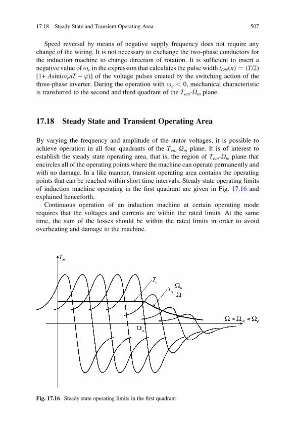
Speed reversal by means of negative supply frequency does not require any
change of the wiring. It is not necessary to exchange the two-phase conductors for
the induction machine to change direction of rotation. It is sufficient to insert a
negative value ofoe in the expression that calculates the pulse width tON(n) ¼ (T/2)[1+ Asin(oenT – ’)] of the voltage pulses created by the switching action of the
three-phase inverter. During the operation with oe < 0, mechanical characteristic
is transferred to the second and third quadrant of the Tem-Om plane.
17.18 Steady State and Transient Operating Area
By varying the frequency and amplitude of the stator voltages, it is possible to
achieve operation in all four quadrants of the Tem-Om plane. It is of interest to
establish the steady state operating area, that is, the region of Tem-Om plane that
encircles all of the operating points where the machine can operate permanently and
with no damage. In a like manner, transient operating area contains the operating
points that can be reached within short time intervals. Steady state operating limits
of induction machine operating in the first quadrant are given in Fig. 17.16 and
explained henceforth.
Continuous operation of an induction machine at certain operating mode
requires that the voltages and currents are within the rated limits. At the same
time, the sum of the losses should be within the rated limits in order to avoid
overheating and damage to the machine.
Fig. 17.16 Steady state operating limits in the first quadrant
17.18 Steady State and Transient Operating Area 507
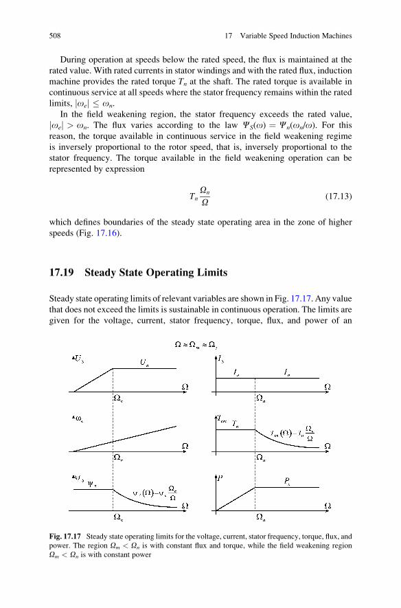
During operation at speeds below the rated speed, the flux is maintained at the
rated value. With rated currents in stator windings and with the rated flux, induction
machine provides the rated torque Tn at the shaft. The rated torque is available in
continuous service at all speeds where the stator frequency remains within the rated
limits, joej � on.
In the field weakening region, the stator frequency exceeds the rated value,
joej > on. The flux varies according to the law CS(o) ¼ Cn(on/o). For this
reason, the torque available in continuous service in the field weakening regime
is inversely proportional to the rotor speed, that is, inversely proportional to the
stator frequency. The torque available in the field weakening operation can be
represented by expression
TnOn
O(17.13)
which defines boundaries of the steady state operating area in the zone of higher
speeds (Fig. 17.16).
17.19 Steady State Operating Limits
Steady state operating limits of relevant variables are shown in Fig. 17.17. Any value
that does not exceed the limits is sustainable in continuous operation. The limits are
given for the voltage, current, stator frequency, torque, flux, and power of an
Fig. 17.17 Steady state operating limits for the voltage, current, stator frequency, torque, flux, and
power. The region Om < On is with constant flux and torque, while the field weakening region
Om < On is with constant power
508 17 Variable Speed Induction Machines
induction machine supplied from variable frequency, variable voltage source. For
clarity of diagrams, it is assumed that O � Oe � Om. The region Om < On below
the rated speed is called constant flux or constant torque region. The regionOm > On
above the rated speed is called flux weakening region or constant power region.Diagrams in Fig. 17.17 represent the change of steady state operating limits for
US, IS, Tem, P, andCS. Therefore, they comprise only the first quadrant with O > 0.
However, the limits such as Tem(Om) apply to all the four quadrants of Tem-Om
plane. Namely, the same limits of the continuous service apply for both directions
of the speed, and they are equally valid in motor operating mode as well as in
generator operating mode. It is shown in the figure that the stator frequency
oe increases proportionally to the rotor speed. By neglecting the slip, relation
between the rotor speed and the stator frequency is oe � pOm. In constant flux
zone, at speeds lower than the rated speed, the ratio US/oe is kept constant. Upon
reaching the rated speed, the voltage is maintained at the rated value. Further
increase of the rotor speed gets the machine in the field weakening mode, where
the voltage remains constant while the angular frequency of the power supply keeps
increasing. This results in flux decrease. In the field weakening regime, the flux
changes according to CS(o) ¼ Cn(on/oe).
In constant flux region, the available torque is constant, while in field weakening
region, the torque is limited by Tem(O) � Tn(On/Oe). The power available in
constant flux region (jOej � On) increases linearly with the speed. In field weaken-
ing, the available torque drops according to Tem ~ 1/O. Therefore, the power
available in field weakening has a constant value, P(O) � OTn(On/O) ¼ Pn.
For this reason, the field weakening region is called constant power region. Byrecognizing the secondary effects, which have been neglected in the first approxi-
mation, it can be shown that the power available in the field weakening regime is
somewhat higher than the rated power.4
17.19.1 RI Compensation
In the process of calculating the stator voltage, the voltage drop across the stator
resistance has been neglected. For clarity, approximation US ¼ RSIS þ joeCS �joeCS has been made. The stator resistance has a very low relative value. There-
fore, this approximation does not introduce any significant error in calculations,
provided that the rotor speeds are sufficiently high and that the electromotive force
oeCS has the value significantly higher than the voltage drop RSIS. At very small
speeds, where the electromotive force is comparable to the voltage drop RSIS, thisapproximation cannot be justified.
4Due to flux decrease in the field weakening regime, the magnetizing current Im is lower than the
rated magnetizing current. This allows for a slight increase in the rotor current liable for the torque
generation.
17.19 Steady State Operating Limits 509
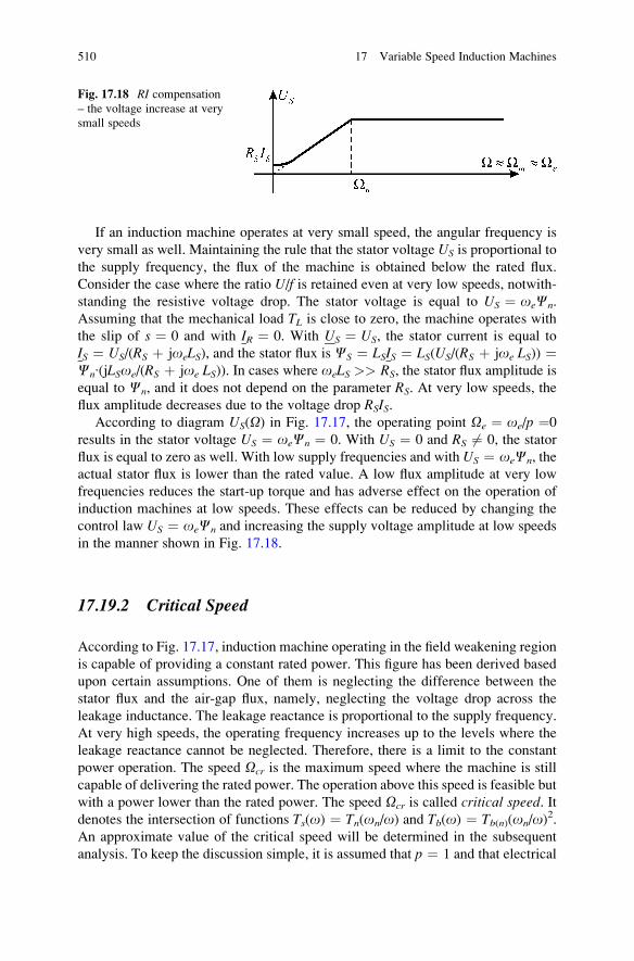
If an induction machine operates at very small speed, the angular frequency is
very small as well. Maintaining the rule that the stator voltage US is proportional to
the supply frequency, the flux of the machine is obtained below the rated flux.
Consider the case where the ratio U/f is retained even at very low speeds, notwith-
standing the resistive voltage drop. The stator voltage is equal to US ¼ oeCn.
Assuming that the mechanical load TL is close to zero, the machine operates with
the slip of s ¼ 0 and with IR ¼ 0. With US ¼ US, the stator current is equal to
IS ¼ US/(RS þ joeLS), and the stator flux is CS ¼ LSIS ¼ LS(US/(RS þ joe LS)) ¼Cn∙(jLSoe/(RS þ joe LS)). In cases where oeLS >> RS, the stator flux amplitude is
equal to Cn, and it does not depend on the parameter RS. At very low speeds, the
flux amplitude decreases due to the voltage drop RSIS.According to diagram US(O) in Fig. 17.17, the operating point Oe ¼ oe/p ¼0
results in the stator voltage US ¼ oeCn ¼ 0. With US ¼ 0 and RS 6¼ 0, the stator
flux is equal to zero as well. With low supply frequencies and with US ¼ oeCn, the
actual stator flux is lower than the rated value. A low flux amplitude at very low
frequencies reduces the start-up torque and has adverse effect on the operation of
induction machines at low speeds. These effects can be reduced by changing the
control law US ¼ oeCn and increasing the supply voltage amplitude at low speeds
in the manner shown in Fig. 17.18.
17.19.2 Critical Speed
According to Fig. 17.17, induction machine operating in the field weakening region
is capable of providing a constant rated power. This figure has been derived based
upon certain assumptions. One of them is neglecting the difference between the
stator flux and the air-gap flux, namely, neglecting the voltage drop across the
leakage inductance. The leakage reactance is proportional to the supply frequency.
At very high speeds, the operating frequency increases up to the levels where the
leakage reactance cannot be neglected. Therefore, there is a limit to the constant
power operation. The speed Ocr is the maximum speed where the machine is still
capable of delivering the rated power. The operation above this speed is feasible but
with a power lower than the rated power. The speed Ocr is called critical speed. Itdenotes the intersection of functions Ts(o) ¼ Tn(on/o) and Tb(o) ¼ Tb(n)(on/o)
2.
An approximate value of the critical speed will be determined in the subsequent
analysis. To keep the discussion simple, it is assumed that p ¼ 1 and that electrical
Fig. 17.18 RI compensation
– the voltage increase at very
small speeds
510 17 Variable Speed Induction Machines
frequencies o have the same values as the relevant speeds O. At the same time, the
slip frequency and the slip speed are considered negligible (oslip << oe, Oslip <<Oe) allowing the rotor speed Om to be replaced with the synchronous speed Oe.
The operation at a constant, rated power in the zone of field weakening requires
the torque Ts(o) � Tn(on/o). The function Ts(o) delimits the steady state operating
limit for the torque. Namely, the curve Ts(o) expresses the maximum steady state
torque at the given speed. The limit torque Ts(o) is obtained with rated stator
current In. On the other hand, the envelope of breakdown torques varies according
to the law Tb(o) � Tb(n)(on/o)2, where Tb(n) is the breakdown torque obtained at
the rated power supply conditions, with the rated flux. The function Tb(o)represents the maximum transient torque available at the given speed. This transient
torque Tb can be maintained only for a short interval of time, as it requires the stator
currents IS > In, and therefore cause increased losses and temperature rise. The
function Ts(o) crosses the function Tb(o) at the speed ocr ¼ on(Tb(n)/Tn).For speeds above ocr, the available breakdown torque Tb(o) is smaller than the
torque Ts(o) � Tn(on/o) which is permissible in continuous service. Hence, the
transient torque limit falls below the torque limit in continuous service, which appears
a contradiction. For the proper understanding, it is of interest to understand the
difference between the functions Ts(o) and Tb(o). The curve Ts(o) represents
the torque Ts which is available at the given speed of o provided that the current in
the stator windings is IS ¼ In. Hence, in a way, the curve Ts(o) represents the limit
IS < In expressed in T(o) plane. It is of interest to notice that the torque values Ts(o)are feasible only in cases where the stator current can actually reach the rated current.
On the other hand, the curve Tb(o) is the actual limit for the instantaneous torque. At
the given speed o, the function Tb(o) provides the peak torque available from the
induction machines of the given parameters. Above critical speeds, the curve Tb(o)provides the values of the breakdown torque available foro > ocr. At the same time,
the values indicated by Ts(o) cannot be reached for speeds o > ocr. At elevated
supply frequencies, the leakage reactance increases. With the stator voltage limited to
the rated value andwith an increased leakage reactance, the stator current cannot reach
the rated values. Hence, for the speeds o > ocr, the stator current falls below In inboth transient and steady state service. This leads to situation where Ts(o) > Tb(o).
Induction machines with variable frequency supply can operate above critical
speed, but their power will fall below the rated power. In this range of speeds, the
available torque will drop proportionally to the square of the rotor speed, while
the available power will drop proportionally the speed, P ~ 1/o. Transient andsteady state operating limits of an induction machine are given in Fig. 17.19.
With the assumed approximations, the critical speed is
Ocr ¼ On1
2xge¼ TbðnÞ
Tn; (17.14)
where
xge ¼ Xge
Zn¼ Lgeon
Zn¼ LgeonIn
Un:
17.19 Steady State Operating Limits 511
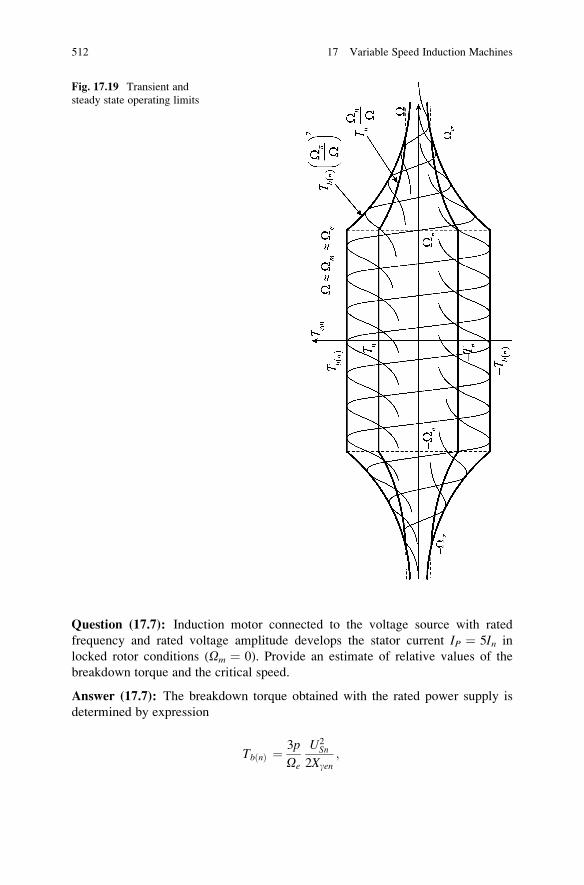
Question (17.7): Induction motor connected to the voltage source with rated
frequency and rated voltage amplitude develops the stator current IP ¼ 5In in
locked rotor conditions (Om ¼ 0). Provide an estimate of relative values of the
breakdown torque and the critical speed.
Answer (17.7): The breakdown torque obtained with the rated power supply is
determined by expression
TbðnÞ ¼ 3p
Oe
U2Sn
2Xgen;
Fig. 17.19 Transient and
steady state operating limits
512 17 Variable Speed Induction Machines
where USn is the rated rms value of the phase voltage, while Xgen is the leakage
inductance at the rated stator frequency. By introducing approximations RS ¼ 0, Lm>> Lge, and (RR/sn) � Un/In >> Xgen, the rated torque can be represented by the
following expression:
Tnom ¼ 3p
Oe
RR
sn
U2Sn
RR
sn
� �2þ X2
gen
� 3p
Oe
RR
sn
U2Sn
RR
sn
� �2 � 3p
Oe
U2Sn
RR
sn
� � � 3p
OeUSnISn;
where sn represents the rated value of the relative slip.
Relative value of the breakdown torque is equal to the ratio of the two preceding
expressions,
mbðnÞ ¼TbðnÞTn
¼U2
Sn
2Xgen
USnISn¼ 1
2xgen;
where xgen is the relative value of the leakage reactance. An approximate value of the
leakage reactance can be determined from the start-up current, xgen � 1/IP ¼ 0.2.
Relative value of the initial torque is equal to mb(n) ¼ 2.5. Critical speed Ocr ¼On(Tb(n)/Tn) is the highest speed at which the rated power can still be obtained.
Relative value of the critical speed (Ocr/On) is equal to the relative value of the
breakdown torque, thus ocr ¼ 2.5on.
17.20 Construction of Induction Machines
Induction machines have been in use since the end of the nineteenth century. During
the first hundred years of their application, the switching power transistors and other
components required for variable frequency supply were not available. For that
reason, induction machines were supplied from the mains, with the voltages having
a constant, line frequency. Therefore, all the induction machines used in this period
were designed and optimized for constant frequency operation. Starting up of the
induction motors was performed by connecting them to a three-phase network of
industrial frequency 50/60 Hz.
17.20.1 Mains-Supplied Machines
At start-up time, a mains-supplied induction motor has the rotor speed Om ¼ 0 and
the stator voltages of the rated amplitude and frequency. The start-up current in the
stator windings is IP � USn/Xge, where Xge � XgS þ XgR is the equivalent leakage
reactance. Small values of the leakage reactance would result in high start-up
17.20 Construction of Induction Machines 513
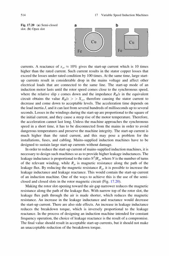
currents. A reactance of xge � 10% gives the start-up current which is 10 times
higher than the rated current. Such current results in the stator copper losses that
exceed the losses under rated condition by 100 times. At the same time, large start-
up currents result in considerable drop in the mains voltage and affect other
electrical loads that are connected to the same line. The start-up mode of an
induction motor lasts until the rotor speed comes close to the synchronous speed,
where the relative slip s comes down and the impedance RR/s in the equivalent
circuit obtains the value RR/s > > Xge, therefore causing the stator current to
decrease and come down to acceptable levels. The acceleration time depends on
the load inertia J, and it can last from several hundreds of milliseconds up to several
seconds. Losses in the windings during the start-up are proportional to the square of
the initial current, and they cause a steep rise of the motor temperature. Therefore,
the acceleration cannot last long. Unless the machine approaches the synchronous
speed in a short time, it has to be disconnected from the mains in order to avoid
dangerous temperatures and preserve the machine integrity. The start-up current is
much higher than the rated current, and this may pose a problem for the
installations, fuses, and cabling. Mains-supplied induction machines have to be
designed to sustain large start-up currents without damage.
In order to reduce the start-up current of mains-supplied induction machines, it is
necessary to design such machines so as to provide higher leakage inductances. The
leakage inductance is proportional to the ratio N2/Rm, where N is the number of turns
of the relevant winding, while Rm is magnetic resistance along the path of the
leakage flux. By reducing the magnetic resistance Rm, it is possible to increase the
leakage inductance and leakage reactance. This would contain the start-up current
of an induction machine. One of the ways to achieve this is the use of the semi-
closed and closed slots in the rotor magnetic circuit (Fig. 17.20).
Making the rotor slot opening toward the air-gap narrower reduces the magnetic
resistance along the path of the leakage flux. With narrow top of the rotor slot, the
leakage flux path through the air is made shorter, which reduces the magnetic
resistance. An increase in the leakage inductance and reactance would decrease
the start-up current. There are also side effects. An increase in leakage inductance
reduces the breakdown torque, which is inversely proportional to the leakage
reactance. In the process of designing an induction machine intended for constant
frequency operation, the choice of leakage reactance is the result of a compromise.
The final value should result in acceptable start-up currents, but it should not make
an unacceptable reduction of the breakdown torque.
Fig. 17.20 (a) Semi-closed
slot. (b) Open slot
514 17 Variable Speed Induction Machines
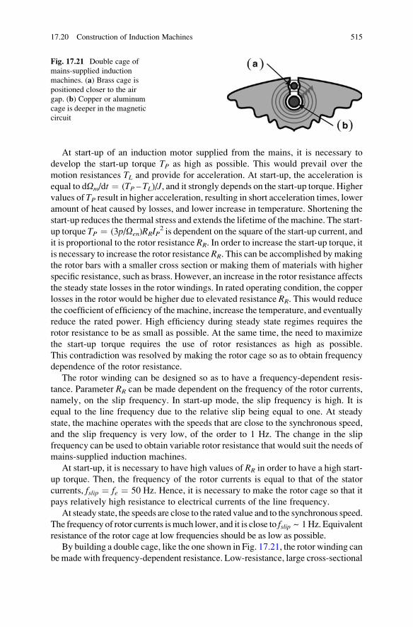
At start-up of an induction motor supplied from the mains, it is necessary to
develop the start-up torque TP as high as possible. This would prevail over the
motion resistances TL and provide for acceleration. At start-up, the acceleration is
equal to dOm/dt ¼ (TP – TL)/J, and it strongly depends on the start-up torque. Highervalues of TP result in higher acceleration, resulting in short acceleration times, lower
amount of heat caused by losses, and lower increase in temperature. Shortening the
start-up reduces the thermal stress and extends the lifetime of the machine. The start-
up torque TP ¼ (3p/Oen)RRIP2 is dependent on the square of the start-up current, and
it is proportional to the rotor resistance RR. In order to increase the start-up torque, it
is necessary to increase the rotor resistance RR. This can be accomplished by making
the rotor bars with a smaller cross section or making them of materials with higher
specific resistance, such as brass. However, an increase in the rotor resistance affects
the steady state losses in the rotor windings. In rated operating condition, the copper
losses in the rotor would be higher due to elevated resistance RR. This would reduce
the coefficient of efficiency of the machine, increase the temperature, and eventually
reduce the rated power. High efficiency during steady state regimes requires the
rotor resistance to be as small as possible. At the same time, the need to maximize
the start-up torque requires the use of rotor resistances as high as possible.
This contradiction was resolved by making the rotor cage so as to obtain frequency
dependence of the rotor resistance.
The rotor winding can be designed so as to have a frequency-dependent resis-
tance. Parameter RR can be made dependent on the frequency of the rotor currents,
namely, on the slip frequency. In start-up mode, the slip frequency is high. It is
equal to the line frequency due to the relative slip being equal to one. At steady
state, the machine operates with the speeds that are close to the synchronous speed,
and the slip frequency is very low, of the order to 1 Hz. The change in the slip
frequency can be used to obtain variable rotor resistance that would suit the needs of
mains-supplied induction machines.
At start-up, it is necessary to have high values of RR in order to have a high start-
up torque. Then, the frequency of the rotor currents is equal to that of the stator
currents, fslip ¼ fe ¼ 50 Hz. Hence, it is necessary to make the rotor cage so that it
pays relatively high resistance to electrical currents of the line frequency.
At steady state, the speeds are close to the rated value and to the synchronous speed.
The frequency of rotor currents ismuch lower, and it is close to fslip ~ 1Hz. Equivalent
resistance of the rotor cage at low frequencies should be as low as possible.
By building a double cage, like the one shown in Fig. 17.21, the rotor winding can
be made with frequency-dependent resistance. Low-resistance, large cross-sectional
Fig. 17.21 Double cage of
mains-supplied induction
machines. (a) Brass cage is
positioned closer to the air
gap. (b) Copper or aluminum
cage is deeper in the magnetic
circuit
17.20 Construction of Induction Machines 515
bars made of copper or aluminum are placed deeper into the rotor magnetic circuit.
This inner cage (B) has much smaller resistance to DC currents. Closer to the
surface, there are brass bars of smaller cross section (A). Their resistance is much
higher. At very low frequencies, such as the rated slip frequencies, the rotor current
has a low-resistance path through the inner cage. At line frequency of 50 Hz, the
inner cage reactance prevents the rotor circuits from passing through the inner cage.
Therefore, the start-up current in the rotor circuit passes through the brass cage,
which is closer to the air gap, which has a much higher resistance and therefore
provides a higher start-up torque.
It is of interest to notice that the leakage reactance of the inner cage is much
higher than the leakage reactance of the brass cage. The figure shows the lines of the
magnetic field of the leakage flux. The copper bars are encircled by a large number
of field lines. For this reason, the leakage flux, leakage inductance, and leakage
reactance are relatively high. The brass cage, placed much closer to the air gap, is
encircled by a smaller number of field lines. Its leakage flux and leakage reactance
are considerably smaller. At start-up, the frequency of rotor currents is fslip ¼ fe¼50 Hz, which increases the values of rotor reactance Xg ¼ Lg oslip ¼ Lg oe. Due
to relatively high frequency, reactances of both cages prevail over resistances, and
the impedance of each of the cages is mainly reactive, Xg >> RR. Since reactance
of the brass cage is considerably smaller, the rotor start-up current passes mainly
through the brass cage, the cage with higher resistance. When the motor enters the
steady state, the frequency of the rotor currents is considerably smaller, and it is
close to fslip ~ 1 Hz. Therefore, the impedance of both cages is mainly resistive, as
the resistances prevail over reactances, Xg ¼ Lg oslip << RR. Since the resistance
of the lower (copper) cage is considerably smaller, the rotor current at steady state
passes mainly through the low-resistance copper bars.
It can be concluded that the rotor currents in a double-cage rotor pass through the
upper, brass cage during start-up, while they get shifted to the lower, copper cage
during operation at steady state, where the speed is close to the synchronous speed
and the slip frequency is low. In this way, the rotor resistance is made frequency
dependent. At steady states close to rated operating conditions, equivalent rotor
resistance is low, while during the start-up, equivalent rotor resistance is high.
Manufacturing double cage increases complexity of the production process and
increases the costs. Therefore, it is used mainly for machines with larger rated
power and/or larger start-up torque requirements.
The effects similar to those created by double cage can be obtained by designing
rotor slots with an increased depth and decreased width. An example of such deep
slot is shown in Fig. 17.22. The slot contains a rotor bar of rectangular cross section.
With very low rotor frequencies, where the leakage reactances are of no impor-
tance, the rotor current is distributed equally across the cross section of the rotor
bar. The currents that pass at the bottom of the slot are encircled by a number of
lines of the magnetic field, that is, by relatively large leakage flux. On the other
hand, there are also currents next to the surface, facing the air gap. They are
encircled by considerably lower number of field lines and have much smaller
leakage flux.
516 17 Variable Speed Induction Machines
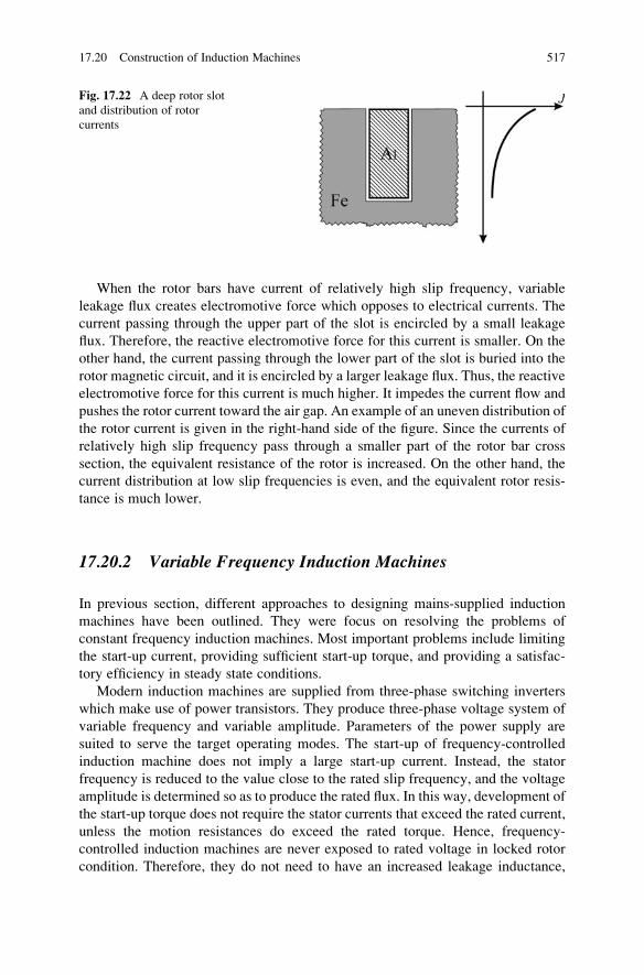
When the rotor bars have current of relatively high slip frequency, variable
leakage flux creates electromotive force which opposes to electrical currents. The
current passing through the upper part of the slot is encircled by a small leakage
flux. Therefore, the reactive electromotive force for this current is smaller. On the
other hand, the current passing through the lower part of the slot is buried into the
rotor magnetic circuit, and it is encircled by a larger leakage flux. Thus, the reactive
electromotive force for this current is much higher. It impedes the current flow and
pushes the rotor current toward the air gap. An example of an uneven distribution of
the rotor current is given in the right-hand side of the figure. Since the currents of
relatively high slip frequency pass through a smaller part of the rotor bar cross
section, the equivalent resistance of the rotor is increased. On the other hand, the
current distribution at low slip frequencies is even, and the equivalent rotor resis-
tance is much lower.
17.20.2 Variable Frequency Induction Machines
In previous section, different approaches to designing mains-supplied induction
machines have been outlined. They were focus on resolving the problems of
constant frequency induction machines. Most important problems include limiting
the start-up current, providing sufficient start-up torque, and providing a satisfac-
tory efficiency in steady state conditions.
Modern induction machines are supplied from three-phase switching inverters
which make use of power transistors. They produce three-phase voltage system of
variable frequency and variable amplitude. Parameters of the power supply are
suited to serve the target operating modes. The start-up of frequency-controlled
induction machine does not imply a large start-up current. Instead, the stator
frequency is reduced to the value close to the rated slip frequency, and the voltage
amplitude is determined so as to produce the rated flux. In this way, development of
the start-up torque does not require the stator currents that exceed the rated current,
unless the motion resistances do exceed the rated torque. Hence, frequency-
controlled induction machines are never exposed to rated voltage in locked rotor
condition. Therefore, they do not need to have an increased leakage inductance,
Fig. 17.22 A deep rotor slot
and distribution of rotor
currents
17.20 Construction of Induction Machines 517
since there is no need to limit the start-up current. Instead, they can be designed to
have open slots of both stator and rotor magnetic circuits, which results in a smaller
leakage flux, smaller leakage inductance, and larger breakdown torque. Example of
an open slot is shown in Fig. 17.20b.
In addition to higher breakdown torque, the advantage obtained by decreasing
leakage inductance is the possibility to achieve faster changes of the stator current,
which results in quicker torque changes. Since the electromagnetic torque of an
electrical machine depends on electrical currents in the windings, the rate of change
of the electromagnetic torque is dependent on the first derivative of the current,
diS(t)/dt. The voltage balance equation in the stator winding can be represented by
uS ¼ RSiS þ LgediS/dt þ e. Therefore, the first derivative of the stator current
diS/dt ¼ (uS – RSiS – e)/Lge is inversely proportional to the leakage inductance.
With lower leakage inductances, it is possible to achieve larger rate of change of the
electromagnetic torque.
Reduction of leakage inductance can also have negative consequences. Due to a
finite number of slots carved into magnetic circuits and due to non-sinusoidal
distribution of conductors, the windings of an induction machine contain
electromotive forces that have higher harmonics. These harmonics cause electrical
currents of the same frequency. The amplitude of such currents in rotor bars is
directly proportional to the amplitudes of the relevant frequency component of the
electromotive force, and inversely proportional to the winding impedance. The
winding impedance at higher frequencies is determined primarily by the leakage
reactance. For this reason, reduction of the leakage inductance leads to increased
amplitudes of winding currents caused by higher harmonics, and increases the
current ripple caused by the PWM supply. The adverse effects can be avoided by
careful design of the rotor slots by shaping the stator and rotor magnetic circuits so
as to reduce non-sinusoidal distribution of the field and to design the stator and rotor
windings so as to reduce the electromotive forces induced due to distortions and
higher harmonics.
Question (17.8): Rotor bars are placed in slots which are separated by teeth. The
lines of the magnetic field are directed along the path of smaller magnetic resis-
tance. Therefore, magnetic induction is high in rotor teeth and significantly lower in
rotor slots. Conductors carrying rotor currents are placed in slots, where magnetic
induction B is close to zero. Considering the force exerted on conductors, it depends
on magnetic induction and electrical current. Apparently, this force is going to be
very low. Explain the fact that, notwithstanding the abovementioned, induction
machine does generate considerable torque.
Answer (17.8): The torque generation can be represented as the result of forces
acting on conductors. With conductors placed in relatively deep slots, magnetic
induction within the iron teeth exceeds by far the magnetic induction within
aluminum-filled slots. Ratio of magnetic induction in slots and magnetic induction
in teeth is close to m0/mFe. Therefore, only a very small force is acting on
conductors. Instead, forces act on rotor surfaces that separate ferromagnetic
materials, such as iron in magnetic circuits, from nonmagnetic materials, such as
518 17 Variable Speed Induction Machines
aluminum conductors or the air gap. They act on the surface walls between slots and
teeth. The forces acting on the rotor teeth can be explained by using the concept
called equivalent magnetic pressure.5 Calculation of spatial distribution of the
magnetic field in relatively complex, three-dimensional structure such as the slotted
rotor is rather involved. In most cases, it requires automated software tools. Once
completed, this calculation provides the information on the equivalent magnetic
pressure which is acting upon surfaces that separate iron from nonmagnetic
domains. With the equivalent magnetic pressure readily available, the forces and
torque can be calculated by performing surface integration along all the relevant
surfaces. The outcome of such calculations is the torque value equal to the value
obtained by assuming that the force LIB acts on each conductor and that magnetic
field lines pass equally through slots as they do through teeth. The last assumption is
equivalent to considering the machine where the rotor surface is smooth cylinder
with no slots, while the rotor conductors reside in the air gap, attached to the rotor
surface. In such hypothetical case, the expression F ¼ LIB is more obvious.
5Magnetic field creates forces acting on surfaces delimiting different domains. These forces can be
described by introducing equivalent pressure p(N/m2). The force acting on surface S is equal to
F ¼ pS. The energy density of the magnetic field in the first domain, next to the boundary, is
w1 ¼ m1 H12/2. Across the boundary, in the second domain, the energy density is w2 ¼ m2 H2
2/2.
Equivalent pressure is equal to w1�w2.
17.20 Construction of Induction Machines 519
Chapter 18
Synchronous Machines
The following chapters study principles of operation, construction, mathematical
model, and basic characteristics of synchronous machines. Along with induction
machines, synchronous machines belong to the group of AC machines. Their
operating principles are different. The rotor of induction machines revolves at the
speed slightly lower than the synchronous speed, thus their name asynchronousmachines. The rotor of synchronous machines revolves at the synchronous speed.
In both induction and synchronous machines, revolving magnetic field is created
by AC currents in the three-phase windings of the stator. The stator magnetic
circuits and the stator windings of induction and synchronous machines are very
much the same. In both cases, three-phase system of stator currents creates rotating
magnetomotive force and rotating field of magnetic inductance. The field revolves
at the speed which is determined by the angular frequency of the stator currents,
also called power supply frequency. Synchronous machines and induction
machines have different construction of their rotors. The rotor winding in most
induction machines is a short-circuited cage made of aluminum bars which are
placed in the rotor slots. Rotor in synchronous machines may have excitation
winding or permanent magnets. The rotor with excitation winding is supplied
with DC currents that create the rotor magnetomotive force and the rotor flux.
Instead of excitation windings, rotor of synchronous machines may have permanent
magnets built into the rotor magnetic circuit. In this case, the rotor does not have
any windings.
The principles of operation of induction machines have been described in
Chap. 14. The rotor windings of an induction machine are short-circuited. When
the rotor of an induction machine falls behind the revolving field by the amount of
slip, the electromotive forces are induced in short-circuited rotor windings, and the
rotor currents appear as a consequence. By joint action of the induced rotor currents
and magnetic field, induction machine generates the electromagnetic torque, pro-
portional to the slip. The torque generation process requires the rotor to revolve
somewhat slower than the field, so that the revolving field advances with respect to
the rotor by the amount of slip. Certain amount of slip is required in order to change
the rotor flux and create electromotive forces and electrical currents in rotor bars.
S.N. Vukosavic, Electrical Machines, Power Electronics and Power Systems,
DOI 10.1007/978-1-4614-0400-2_18, # Springer Science+Business Media New York 2013
521
It has been shown in Chap. 14 that electromagnetic torque of an induction machine
depends on the angular frequency of rotor currents oslip ¼ oe-pOm, which is
determined by the rotor lagging with respect to revolving field. In rated operating
conditions, the rotor of an induction machine does not rotate synchronously with
the field. Therefore, induction machines are also called asynchronous machines.Rotor in synchronous machines is either an electromagnet or a permanent
magnet. Position of the rotor flux is uniquely defined by the position of the rotor.
In rated operating conditions, the rotor revolves synchronously with the stator field.
Electromagnetic torque is proportional to the vector product of the stator and rotor
flux vectors. The synchronous rotation of the rotor is the reason for this type of
electrical machines to be called synchronous machines.In this chapter, basic operating principles of synchronous machines are
introduced and explained. The torque generation is discussed for the machines
with an excitation winding on the rotor and for the machines with permanent
magnets. The construction of stator windings and stator magnetic circuit is rather
similar to that of the induction machine. It is reinstated briefly, along with genera-
tion of the revolving magnetic field of the stator winding. The rotor construction is
explained in more detail. The available methods of supplying the DC excitation
current to rotors with an excitation winding are introduced, explained, and
discussed, including the sliding rings with brushes and the transformer with
revolving secondary and rectifier circuit on the rotor. This chapter reviews most
significant characteristics of permanent magnet materials. Two different ways of
inserting permanent magnets into the rotor magnetic circuits are explained and
discussed. Magnetic and electrical properties of synchronous machines with buried
magnets and surface-mounted magnets are studied. In particular, the difference in
self-inductance of the stator windings is discussed and explained for buried magnet
machines and surface-mounted magnet machines.
18.1 Principle of Operation
Like induction machines, synchronous machines have AC currents in stator
windings. Stator currents create the stator magnetomotive force FS which revolves
at the speed Oe ¼ oe/p, also called synchronous speed. The synchronous speed is
determined by the angular frequencyoe of stator currents and by the number of pole
pairs p. The stator magnetomotive force creates the stator flux FS ¼ FS/Rm, which
depends on magnetic resistance Rm. The fluxFS rotates at the same speed Oe as the
magnetomotive force. Rotor in synchronous machines may have permanent
magnets built into magnetic circuit or excitation windings supplied by DC current.
In both cases, the rotor flux FR has the course and direction determined by the rotor
position. The flux vector FR rotates at the rotor speed Om. With Om ¼ Oe, both the
stator flux vector FS and the rotor flux vector FR revolve at the same speed. They
do not change their relative position and maintain the angle between the two vectors
constant. The torque and power of electromechanical conversion are dependent on
522 18 Synchronous Machines
the vector product of the two flux vectors. The vector product depends on the angle
between the two vectors. With Om ¼ Oe, the two flux vectors do not change their
relative position. The electromagnetic torque is proportional to the product of the
two flux amplitudes and to the sine of the angle between the two flux vectors. With
constant flux amplitudes and constant relative position between the two flux
vectors, the electromagnetic torque remains constant. The operation of synchronous
machines and the torque development require synchronous rotation (Om ¼ Oe) of
the stator field, created by the stator currents, and the rotor field, created by
excitation winding or permanent magnets.
18.2 Stator Windings
Stator of a synchronous machine is very much the same as the stator of an induction
machine. Current circuits on the stator side have three separate parts called stator
phase windings or stator phases. Each phase is obtained by connecting a number of
turns in series. Relevant conductors are distributed along the machine circumfer-
ence and placed into slots. The stator slots are carved into the inner side of the stator
magnetic circuit, facing the air gap. Distribution of stator conductors along the
machine circumference is quasisinusoidal. That is, an attempt is made to achieve
sinusoidal change of the conductor density along the circumference. Ideal sinusoi-
dal distribution cannot be achieved due to a finite number of slots. Conductors
cannot be placed in an arbitrary position. They have to be placed in one of the slots.
Hence, there are a limited number of discrete locations for the placement of stator
conductors. For this reason, sinusoidal distribution of stator conductors along the
machine circumference cannot be achieved in full. Yet, the windings are made in
such way that the distribution of conductors gets as close to sinusoidal as possible.
Each of the three-phase windings has two terminals. One end of each phase winding
is connected to the three-phase voltage source which supplies the stator windings.
Stator terminals of synchronous generators may be connected to three-phase elec-
trical loads. Remaining ends of the three-phase windings are wired together into the
node called star point. This way of connecting the stator phases is called starconnection. With the sum of the three-phase currents equal to zero, ia(t) þ ib(t) þic(t) ¼ 0, there is no need to connect the star point to the source; thus, no return line
is required. Most machines1 have their star points disconnected from the power
1 Electrical machines supplied the mains with line voltages U < 1 kV are also called low-voltage
machines. Most low-voltage machines have star connected stator windings with floating star point.
Namely, the star connection of the three phases is not connected to any other node. In most cases,
the star point is even inaccessible, namely, it is not made available to the user. Machines with
stator voltages in excess to 1 kV may have their star point connected to the neutral or to the ground
by means of a series impedance. This connection reduces the overvoltage stress. In most cases, the
impedance used for grounding the star point has a minor effect on the equation ia þ ib þ ic ¼ 0.
18.2 Stator Windings 523
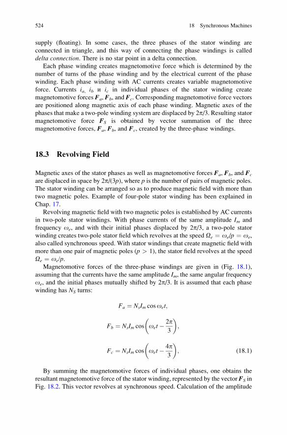
supply (floating). In some cases, the three phases of the stator winding are
connected in triangle, and this way of connecting the phase windings is called
delta connection. There is no star point in a delta connection.
Each phase winding creates magnetomotive force which is determined by the
number of turns of the phase winding and by the electrical current of the phase
winding. Each phase winding with AC currents creates variable magnetomotive
force. Currents ia, ib и ic in individual phases of the stator winding create
magnetomotive forces Fa, Fb, and Fc. Corresponding magnetomotive force vectors
are positioned along magnetic axis of each phase winding. Magnetic axes of the
phases that make a two-pole winding system are displaced by 2p/3. Resulting statormagnetomotive force FS is obtained by vector summation of the three
magnetomotive forces, Fa, Fb, and Fc, created by the three-phase windings.
18.3 Revolving Field
Magnetic axes of the stator phases as well as magnetomotive forces Fa, Fb, and Fc
are displaced in space by 2p/(3p), where p is the number of pairs of magnetic poles.
The stator winding can be arranged so as to produce magnetic field with more than
two magnetic poles. Example of four-pole stator winding has been explained in
Chap. 17.
Revolving magnetic field with two magnetic poles is established by AC currents
in two-pole stator windings. With phase currents of the same amplitude Im and
frequency oe, and with their initial phases displaced by 2p/3, a two-pole stator
winding creates two-pole stator field which revolves at the speed Oe ¼ oe/p ¼ oe,
also called synchronous speed. With stator windings that create magnetic field with
more than one pair of magnetic poles (p > 1), the stator field revolves at the speed
Oe ¼ oe/p.Magnetomotive forces of the three-phase windings are given in (Fig. 18.1),
assuming that the currents have the same amplitude Im, the same angular frequency
oe, and the initial phases mutually shifted by 2p/3. It is assumed that each phase
winding has NS turns:
Fa ¼ NsIm cosoet;
Fb ¼ NsIm cos oet� 2p3
� �;
Fc ¼ NsIm cos oet� 4p3
� �; (18.1)
By summing the magnetomotive forces of individual phases, one obtains the
resultant magnetomotive force of the stator winding, represented by the vector FS in
Fig. 18.2. This vector revolves at synchronous speed. Calculation of the amplitude
524 18 Synchronous Machines
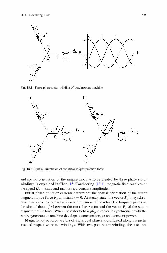
and spatial orientation of the magnetomotive force created by three-phase stator
windings is explained in Chap. 15. Considering (18.1), magnetic field revolves at
the speed Oe ¼ oe/p and maintains a constant amplitude.
Initial phase of stator currents determines the spatial orientation of the stator
magnetomotive force FS at instant t ¼ 0. At steady state, the vector FS in synchro-
nous machines has to revolve in synchronism with the rotor. The torque depends on
the sine of the angle between the rotor flux vector and the vector FS of the stator
magnetomotive force. When the stator field FS/Rm revolves in synchronism with the
rotor, synchronous machine develops a constant torque and constant power.
Magnetomotive force vectors of individual phases are oriented along magnetic
axes of respective phase windings. With two-pole stator winding, the axes are
Fig. 18.2 Spatial orientation of the stator magnetomotive force
Fig. 18.1 Three-phase stator winding of synchronous machine
18.3 Revolving Field 525
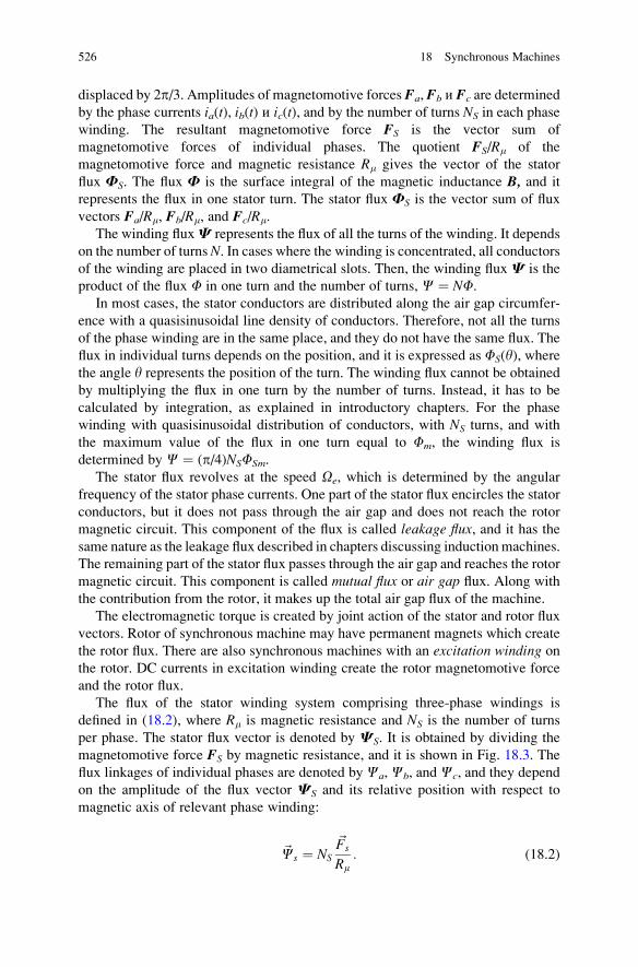
displaced by 2p/3. Amplitudes of magnetomotive forces Fa, Fb и Fc are determined
by the phase currents ia(t), ib(t) и ic(t), and by the number of turns NS in each phase
winding. The resultant magnetomotive force FS is the vector sum of
magnetomotive forces of individual phases. The quotient FS/Rm of the
magnetomotive force and magnetic resistance Rm gives the vector of the stator
flux FS. The flux F is the surface integral of the magnetic inductance B, and it
represents the flux in one stator turn. The stator flux FS is the vector sum of flux
vectors Fa/Rm, Fb/Rm, and Fc/Rm.
The winding fluxC represents the flux of all the turns of the winding. It depends
on the number of turns N. In cases where the winding is concentrated, all conductorsof the winding are placed in two diametrical slots. Then, the winding flux C is the
product of the flux F in one turn and the number of turns, C ¼ NF.In most cases, the stator conductors are distributed along the air gap circumfer-
ence with a quasisinusoidal line density of conductors. Therefore, not all the turns
of the phase winding are in the same place, and they do not have the same flux. The
flux in individual turns depends on the position, and it is expressed as FS(y), wherethe angle y represents the position of the turn. The winding flux cannot be obtainedby multiplying the flux in one turn by the number of turns. Instead, it has to be
calculated by integration, as explained in introductory chapters. For the phase
winding with quasisinusoidal distribution of conductors, with NS turns, and with
the maximum value of the flux in one turn equal to Fm, the winding flux is
determined by C ¼ (p/4)NSFSm.
The stator flux revolves at the speed Oe, which is determined by the angular
frequency of the stator phase currents. One part of the stator flux encircles the stator
conductors, but it does not pass through the air gap and does not reach the rotor
magnetic circuit. This component of the flux is called leakage flux, and it has the
same nature as the leakage flux described in chapters discussing induction machines.
The remaining part of the stator flux passes through the air gap and reaches the rotor
magnetic circuit. This component is called mutual flux or air gap flux. Along with
the contribution from the rotor, it makes up the total air gap flux of the machine.
The electromagnetic torque is created by joint action of the stator and rotor flux
vectors. Rotor of synchronous machine may have permanent magnets which create
the rotor flux. There are also synchronous machines with an excitation winding on
the rotor. DC currents in excitation winding create the rotor magnetomotive force
and the rotor flux.
The flux of the stator winding system comprising three-phase windings is
defined in (18.2), where Rm is magnetic resistance and NS is the number of turns
per phase. The stator flux vector is denoted by CS. It is obtained by dividing the
magnetomotive force FS by magnetic resistance, and it is shown in Fig. 18.3. The
flux linkages of individual phases are denoted by Ca, Cb, and Cc, and they depend
on the amplitude of the flux vector CS and its relative position with respect to
magnetic axis of relevant phase winding:
~Cs ¼ NS
~Fs
Rm: (18.2)
526 18 Synchronous Machines
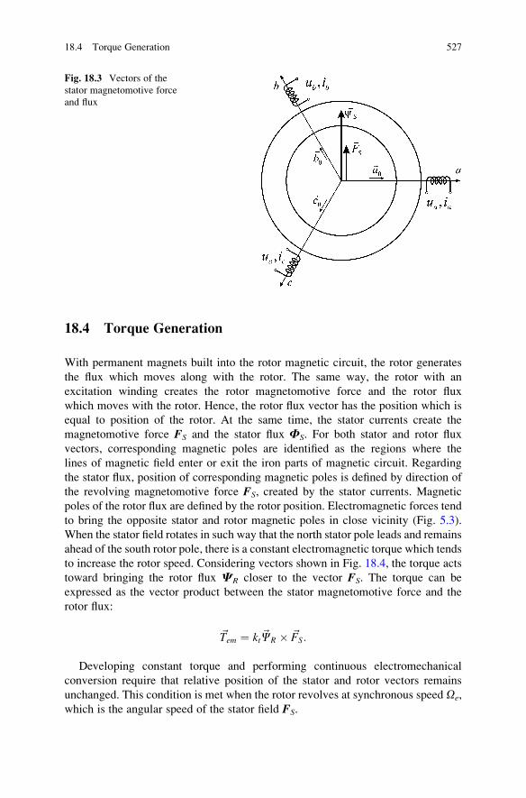
18.4 Torque Generation
With permanent magnets built into the rotor magnetic circuit, the rotor generates
the flux which moves along with the rotor. The same way, the rotor with an
excitation winding creates the rotor magnetomotive force and the rotor flux
which moves with the rotor. Hence, the rotor flux vector has the position which is
equal to position of the rotor. At the same time, the stator currents create the
magnetomotive force FS and the stator flux FS. For both stator and rotor flux
vectors, corresponding magnetic poles are identified as the regions where the
lines of magnetic field enter or exit the iron parts of magnetic circuit. Regarding
the stator flux, position of corresponding magnetic poles is defined by direction of
the revolving magnetomotive force FS, created by the stator currents. Magnetic
poles of the rotor flux are defined by the rotor position. Electromagnetic forces tend
to bring the opposite stator and rotor magnetic poles in close vicinity (Fig. 5.3).
When the stator field rotates in such way that the north stator pole leads and remains
ahead of the south rotor pole, there is a constant electromagnetic torque which tends
to increase the rotor speed. Considering vectors shown in Fig. 18.4, the torque acts
toward bringing the rotor flux CR closer to the vector FS. The torque can be
expressed as the vector product between the stator magnetomotive force and the
rotor flux:
~Tem ¼ kt~CR � ~FS:
Developing constant torque and performing continuous electromechanical
conversion require that relative position of the stator and rotor vectors remains
unchanged. This condition is met when the rotor revolves at synchronous speed Oe,
which is the angular speed of the stator field FS.
Fig. 18.3 Vectors of the
stator magnetomotive force
and flux
18.4 Torque Generation 527
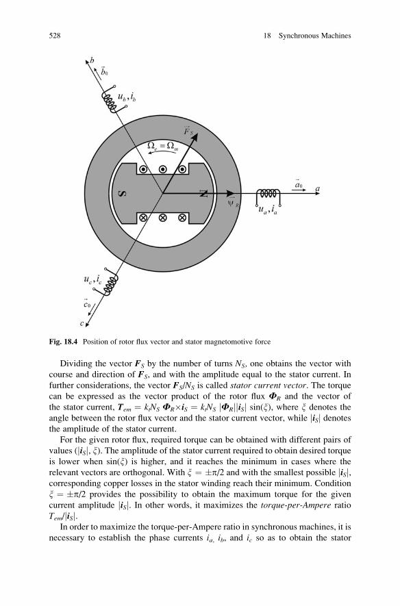
Dividing the vector FS by the number of turns NS, one obtains the vector with
course and direction of FS, and with the amplitude equal to the stator current. In
further considerations, the vector FS/NS is called stator current vector. The torquecan be expressed as the vector product of the rotor flux FR and the vector of
the stator current, Tem ¼ ktNS FR�iS ¼ ktNS jFRjjiSj sin(x), where x denotes the
angle between the rotor flux vector and the stator current vector, while jiSj denotesthe amplitude of the stator current.
For the given rotor flux, required torque can be obtained with different pairs of
values (jiSj, x). The amplitude of the stator current required to obtain desired torque
is lower when sin(x) is higher, and it reaches the minimum in cases where the
relevant vectors are orthogonal. With x ¼ �p/2 and with the smallest possible jiSj,corresponding copper losses in the stator winding reach their minimum. Condition
x ¼ �p/2 provides the possibility to obtain the maximum torque for the given
current amplitude jiSj. In other words, it maximizes the torque-per-Ampere ratio
Tem/jiSj.In order to maximize the torque-per-Ampere ratio in synchronous machines, it is
necessary to establish the phase currents ia, ib, and ic so as to obtain the stator
Fig. 18.4 Position of rotor flux vector and stator magnetomotive force
528 18 Synchronous Machines
magnetomotive force vector FS which is perpendicular to the rotor flux. Hence,
whatever the rotor speed or position, the vector FS is to be locked to the rotor
position, advancing with respect to the rotor flux by p/2. In such cases, the
electromagnetic torque is determined by the amplitude of the stator current, Tem ¼ktNS jFRjjiSj. Negative values of the torque are obtained when the vector FS falls
behind the rotor flux by p/2. This approach is used in controlling the torque of
permanent magnet synchronous machines used in motion control applications.
These synchronous machines are also called synchronous servomotors, and they
are distinguished by low inertia of the rotor and high ratio of the peak torque and the
rated torque. In motion control applications, each synchronous servomotor is
supplied from a separate three-phase inverter which supplies the motors with the
phase currents required for generating the set torque. By using the current regulator
with pulse width modulation control, the stator voltages are adjusted so as to obtain
desired phase currents ia, ib, and ic. Three-phase inverters with pulse with modula-
tion and with current regulator are also called current regulated pulse widthmodulated inverters or CRPWM inverters.
Question (18.1): Consider two induction machines with short-circuited rotor cage
and with the same dimensions of stator and rotor magnetic circuits. One of these is a
two-pole induction machine while the other is a four-pole machine. The rotors of
both machines are taken out of their stators. A new machine is made by inserting the
rotor of the second machine into the stator of the first machine. Is it possible for the
new machine to develop any torque?
Answer (18.1): The torque development is based on interaction of the stator and
rotor magnetic fields. In order to obtain the electromagnetic torque, it is necessary
that the rotor and stator fields have the same number of magnetic poles. Magnetic
field of the stator of an induction machine is created by magnetomotive forces
caused by electrical currents in the stator windings. The stator windings of the first
machine generate a two-pole magnetic field, while the stator windings of the second
machine create a four-pole magnetic field. The latter has two north magnetic poles
and two south magnetic poles. In both machines, magnetic field of the rotor depends
on the currents induced in the rotor conductors. The rotor currents appear as a
consequence of electromotive forces induced in the rotor cage. Electromotive
forces depend on magnetic induction in the air gap, and they also depend on the
slip speed. The change in amplitude and direction of the rotor electromotive forces
and currents reflects the change of the air gap inductance B. Therefore, the number
of magnetic poles of consequential rotor flux is the same as the number of poles of
the stator magnetic field. Hence, one and the same rotor creates a two-pole field
while operating within a two-pole stator and a four-pole field when operating in a
four-pole stator. Therefore, the machine made by combining the stator of the first
machine with the rotor of the second machine will be capable of running as a proper
induction machine, and it will develop the torque.
Question (18.2): Consider two synchronous machines, each with permanent
magnet rotor. Bothmachines have equal dimensions of their rotor and statormagnetic
18.4 Torque Generation 529
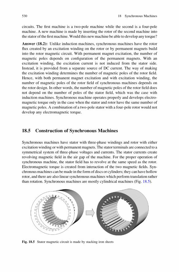
circuits. The first machine is a two-pole machine while the second is a four-pole
machine. A new machine is made by inserting the rotor of the second machine into
the stator of the firstmachine.Would this newmachine be able to develop any torque?
Answer (18.2): Unlike induction machines, synchronous machines have the rotor
flux created by an excitation winding on the rotor or by permanent magnets build
into the rotor magnetic circuit. With permanent magnet excitation, the number of
magnetic poles depends on configuration of the permanent magnets. With an
excitation winding, the excitation current is not induced from the stator side.
Instead, it is provided from a separate source of DC current. The way of making
the excitation winding determines the number of magnetic poles of the rotor field.
Hence, with both permanent magnet excitation and with excitation winding, the
number of magnetic poles of the rotor field of synchronous machines depends on
the rotor design. In other words, the number of magnetic poles of the rotor field does
not depend on the number of poles of the stator field, which was the case with
induction machines. Synchronous machine operates properly and develops electro-
magnetic torque only in the case when the stator and rotor have the same number of
magnetic poles. A combination of a two-pole stator with a four-pole rotor would not
develop any electromagnetic torque.
18.5 Construction of Synchronous Machines
Synchronous machines have stator with three-phase windings and rotor with either
excitationwinding orwith permanentmagnets. The stator terminals are connected to a
symmetrical system of three-phase voltages and currents. The stator currents create
revolving magnetic field in the air gap of the machine. For the proper operation of
synchronous machine, the stator field has to revolve at the same speed as the rotor.
Electromagnetic torque is created from interaction of the two magnetic fields. Syn-
chronousmachines can bemade in the formof discs or cylinders; they can have hollow
rotor, and there are also linear synchronous machines which perform translation rather
than rotation. Synchronous machines are mostly cylindrical machines (Fig. 18.5).
Fig. 18.5 Stator magnetic circuit is made by stacking iron sheets
530 18 Synchronous Machines
18.6 Stator Magnetic Circuit
Stator of cylindrical synchronousmachines is a hollow cylinder which accommodates
the rotor. The main parts of the stator are magnetic circuit and current circuits, also
called phase windings. Magnetic circuit is made of ferromagnetic materials, usually
iron alloys, while the current circuits consist of insulated copper conductors.
Stator of synchronous machines is entirely the same as the stator of an induction
machine. Magnetic induction B in the stator magnetic circuit changes due to
rotation of the magnetic field with respect to the stator core. Induction B varies
with the frequency oe, which is the angular frequency of the stator currents.
Variation of magnetic induction causes eddy current losses and hysteresis losses
in conductive ferromagnetics. The losses due to eddy currents are proportional to
the square of the frequency, while the losses due to hysteresis are proportional to the
frequency. In synchronous machines supplied from the mains, magnetic induction
in the stator magnetic circuit pulsates at the frequency of fe ¼ 50 Hz (60 Hz). In
order to reduce losses in the stator magnetic circuit, it is made by stacking the iron
sheets. The sheets are separated by a thin layer of electric insulation.
The iron sheets are actually made of iron alloys comprising small quantities of
manganese and other elements. Lamination of magnetic circuit does not reduce the
hysteresis losses, but it suppresses the eddy currents and reduces the overall iron
losses in magnetic circuit caused by the pulsation of magnetic induction. Since the
magnetic field revolves with respect to the stator, magnetic induction in stator
magnetic circuit changes direction. For this reason, it is essential for the iron sheets
to have the samemagnetic properties in all directions. Such sheets are obtained by hotrolling of steel, and they are called hot rolled sheets. On the other hand, magnetic
circuits used in power transformers have the field which is always directed along the
same path. Therefore, it is important to have improved magnetic properties along the
flux path, while the properties in directions perpendicular to the path are of lesser
importance. In such cases, it is beneficial to use anisotropic2 material, optimized to
provide a lowmagnetic resistance along the flux path. The sheets with such properties
are obtained by cold rolling. Hence, the iron sheets used in power transformers
are cold rolled sheets. Cold rolling results in reducedmagnetic resistance in direction
of rolling, which should correspond to the flux path within power transformer.
By stacking the sheets, one obtains a hollow cylinder with slots on the inner
surface which faces the air gap. The slots are intended for placing conductors of the
stator winding. Parts of the stator magnetic circuit between the slots are called teeth.
The flux passing toward the air gap is directed through the teeth, made of iron of
high-permeability and low magnetic resistance. The flux does not pass through the
slots, where permeability is m0 and where magnetic resistance is high. Therefore,
magnetic induction inside teeth is higher compared to the rest of the stator magnetic
circuit, which results in increased teeth iron losses.
2 Anisotropic – having different properties in different directions. For example, anisotropic
ferromagnetic may have different permeability in direction of axes x, y, and z.
18.6 Stator Magnetic Circuit 531
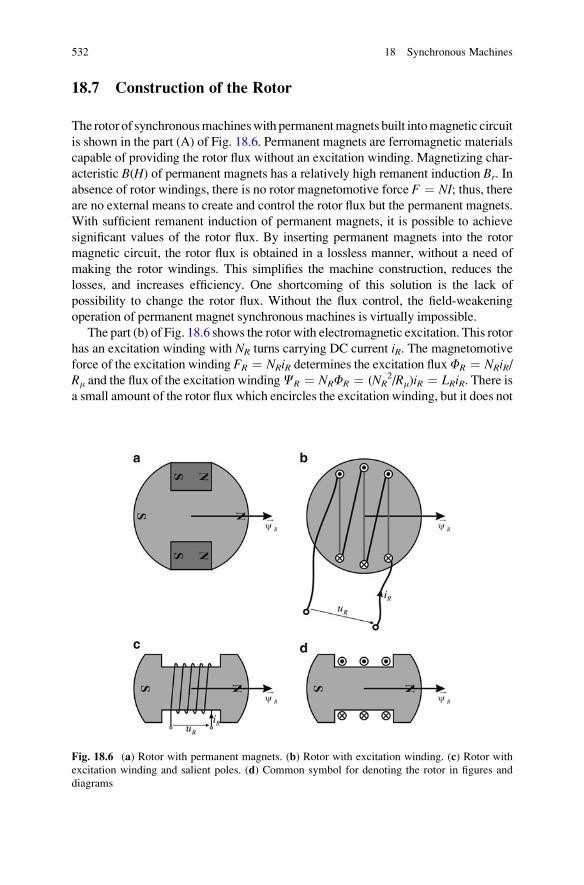
18.7 Construction of the Rotor
The rotor of synchronousmachineswith permanentmagnets built intomagnetic circuit
is shown in the part (A) of Fig. 18.6. Permanent magnets are ferromagnetic materials
capable of providing the rotor flux without an excitation winding. Magnetizing char-
acteristic B(H) of permanent magnets has a relatively high remanent induction Br. In
absence of rotor windings, there is no rotor magnetomotive force F ¼ NI; thus, thereare no external means to create and control the rotor flux but the permanent magnets.
With sufficient remanent induction of permanent magnets, it is possible to achieve
significant values of the rotor flux. By inserting permanent magnets into the rotor
magnetic circuit, the rotor flux is obtained in a lossless manner, without a need of
making the rotor windings. This simplifies the machine construction, reduces the
losses, and increases efficiency. One shortcoming of this solution is the lack of
possibility to change the rotor flux. Without the flux control, the field-weakening
operation of permanent magnet synchronous machines is virtually impossible.
The part (b) of Fig. 18.6 shows the rotor with electromagnetic excitation. This rotor
has an excitation winding with NR turns carrying DC current iR. The magnetomotive
force of the excitation winding FR ¼ NRiR determines the excitation fluxFR ¼ NRiR/Rm and the flux of the excitation windingCR ¼ NRFR ¼ (NR
2/Rm)iR ¼ LRiR. There isa small amount of the rotor flux which encircles the excitation winding, but it does not
Fig. 18.6 (a) Rotor with permanent magnets. (b) Rotor with excitation winding. (c) Rotor with
excitation winding and salient poles. (d) Common symbol for denoting the rotor in figures and
diagrams
532 18 Synchronous Machines
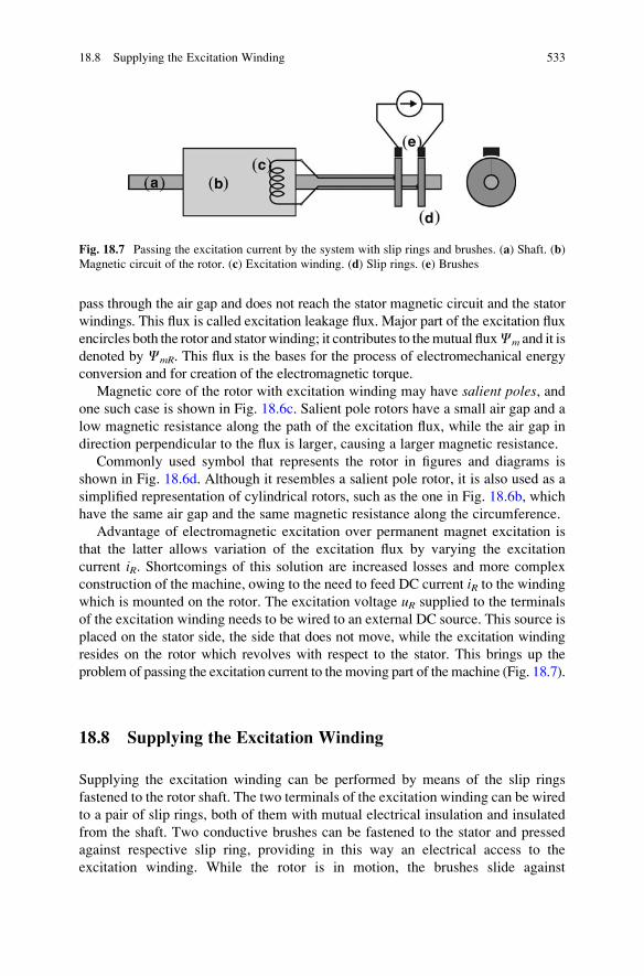
pass through the air gap and does not reach the stator magnetic circuit and the stator
windings. This flux is called excitation leakage flux. Major part of the excitation flux
encircles both the rotor and statorwinding; it contributes to themutual fluxCm and it is
denoted by CmR. This flux is the bases for the process of electromechanical energy
conversion and for creation of the electromagnetic torque.
Magnetic core of the rotor with excitation winding may have salient poles, andone such case is shown in Fig. 18.6c. Salient pole rotors have a small air gap and a
low magnetic resistance along the path of the excitation flux, while the air gap in
direction perpendicular to the flux is larger, causing a larger magnetic resistance.
Commonly used symbol that represents the rotor in figures and diagrams is
shown in Fig. 18.6d. Although it resembles a salient pole rotor, it is also used as a
simplified representation of cylindrical rotors, such as the one in Fig. 18.6b, which
have the same air gap and the same magnetic resistance along the circumference.
Advantage of electromagnetic excitation over permanent magnet excitation is
that the latter allows variation of the excitation flux by varying the excitation
current iR. Shortcomings of this solution are increased losses and more complex
construction of the machine, owing to the need to feed DC current iR to the windingwhich is mounted on the rotor. The excitation voltage uR supplied to the terminals
of the excitation winding needs to be wired to an external DC source. This source is
placed on the stator side, the side that does not move, while the excitation winding
resides on the rotor which revolves with respect to the stator. This brings up the
problem of passing the excitation current to the moving part of the machine (Fig. 18.7).
18.8 Supplying the Excitation Winding
Supplying the excitation winding can be performed by means of the slip rings
fastened to the rotor shaft. The two terminals of the excitation winding can be wired
to a pair of slip rings, both of them with mutual electrical insulation and insulated
from the shaft. Two conductive brushes can be fastened to the stator and pressed
against respective slip ring, providing in this way an electrical access to the
excitation winding. While the rotor is in motion, the brushes slide against
Fig. 18.7 Passing the excitation current by the system with slip rings and brushes. (a) Shaft. (b)
Magnetic circuit of the rotor. (c) Excitation winding. (d) Slip rings. (e) Brushes
18.8 Supplying the Excitation Winding 533
the rings and maintain electrical contact. DC current fed to the brushes passes to the
slip rings and gets to the terminals of the excitation winding. Prescribed method of
supplying the excitation winding from the stator side passes the DC current from an
external source to the excitation winding. It works both with the rotor in motion and
with the rotor at standstill. By changing the excitation voltage, the excitation
current can be adjusted so as to provide the rotor flux that corresponds to desired
operating mode of the machine.
Large hydrogenerators that operate in hydroelectric power plants as well as
turbogenerators that operate in thermal power plants have electromagnetic excita-
tion that includes the excitation winding on the rotor. Electrical current in excitation
winding is adjusted so as to obtain desired voltage across the stator terminals.
The stator electromotive force determines the stator voltage. At the same time, the
electromotive force is proportional to the rotor flux. Hence, the stator voltage of
synchronous generators can be increased or decreased by changing the excitation
current. Variation of generator voltages is required in order to compensate for
variable voltage drops between the power plants and electrical consumers. As the
consumption of electrical power at the consumer side increases, the generator load
increases as well as the stator current. An increased current produces larger voltage
drops in transmission lines, power transformers, and distribution cables. In order to
keep the consumer voltages constant, it is necessary to increase the voltage of
synchronous generators. This increase is required to compensate for the increased
voltage drops in transmission and distribution. The goal is achieved by increasing
the excitation current of synchronous generators.
One shortcoming of the excitation system with slip rings is that the excitation
current passes through the contact between the brushes and slip rings. The rotormotion
makes the contact surfaces slide against each other. With unsteady electrical contact,
electric arcmay app7ear in the course of rotation. Sporadic arcing presents the fire risk
and increases electromagnetic interference. Besides, arcing and friction contribute to
ware of the sliding rings and brushes. This in turn requires repairs and maintenance.
Besides, the presence of slip rings increases the axial length of the machine.
18.9 Excitation with Rotating Transformer
The transfer of the excitation power to the rotor without mechanical contact can be
accomplished by using a rotating transformer, the principles of which are depicted
in Fig. 18.8. Primary winding of this transformer is on the stator side of the
machine, along with one half of the transformer magnetic circuit. Both transformer
parts are attached to the stator and do not move. The stator side of the
transformer magnetic circuit has the shape of a ring. Along the circumference, a
slot is carved into the inner surface of the ring, and the primary winding is placed
into this slot. The other part of the transformer magnetic circuit is attached to the
rotor shaft, and it moves with the rotor. It has the shape of a ring of a smaller
diameter so that it fits into the stator part of the transformer magnetic circuit. A slot
534 18 Synchronous Machines
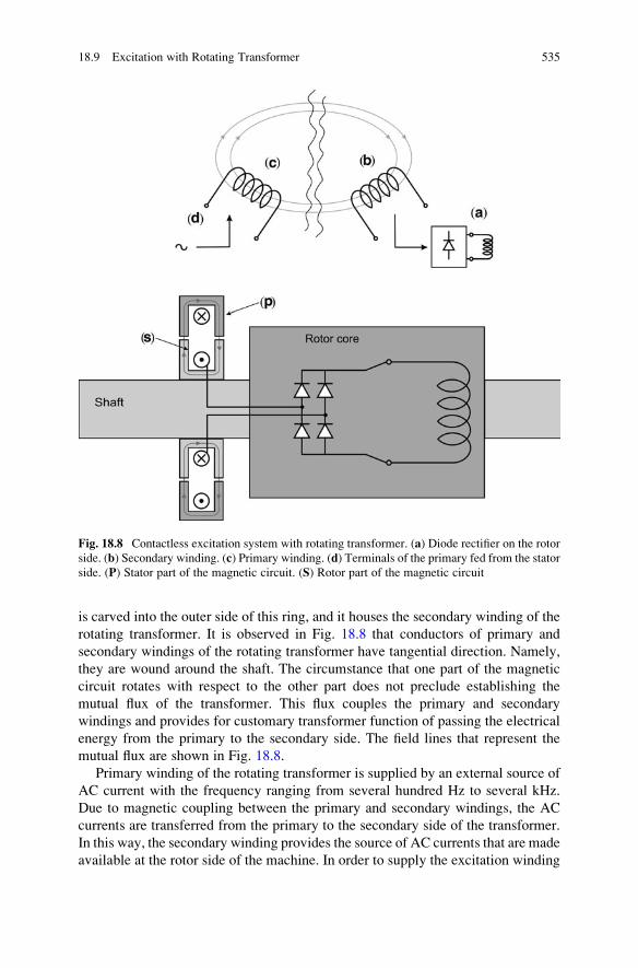
is carved into the outer side of this ring, and it houses the secondary winding of the
rotating transformer. It is observed in Fig. 18.8 that conductors of primary and
secondary windings of the rotating transformer have tangential direction. Namely,
they are wound around the shaft. The circumstance that one part of the magnetic
circuit rotates with respect to the other part does not preclude establishing the
mutual flux of the transformer. This flux couples the primary and secondary
windings and provides for customary transformer function of passing the electrical
energy from the primary to the secondary side. The field lines that represent the
mutual flux are shown in Fig. 18.8.
Primary winding of the rotating transformer is supplied by an external source of
AC current with the frequency ranging from several hundred Hz to several kHz.
Due to magnetic coupling between the primary and secondary windings, the AC
currents are transferred from the primary to the secondary side of the transformer.
In this way, the secondary winding provides the source of AC currents that are made
available at the rotor side of the machine. In order to supply the excitation winding
Fig. 18.8 Contactless excitation system with rotating transformer. (a) Diode rectifier on the rotor
side. (b) Secondary winding. (c) Primary winding. (d) Terminals of the primary fed from the stator
side. (P) Stator part of the magnetic circuit. (S) Rotor part of the magnetic circuit
18.9 Excitation with Rotating Transformer 535
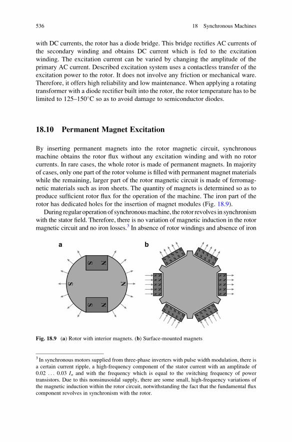
with DC currents, the rotor has a diode bridge. This bridge rectifies AC currents of
the secondary winding and obtains DC current which is fed to the excitation
winding. The excitation current can be varied by changing the amplitude of the
primary AC current. Described excitation system uses a contactless transfer of the
excitation power to the rotor. It does not involve any friction or mechanical ware.
Therefore, it offers high reliability and low maintenance. When applying a rotating
transformer with a diode rectifier built into the rotor, the rotor temperature has to be
limited to 125–150�C so as to avoid damage to semiconductor diodes.
18.10 Permanent Magnet Excitation
By inserting permanent magnets into the rotor magnetic circuit, synchronous
machine obtains the rotor flux without any excitation winding and with no rotor
currents. In rare cases, the whole rotor is made of permanent magnets. In majority
of cases, only one part of the rotor volume is filled with permanent magnet materials
while the remaining, larger part of the rotor magnetic circuit is made of ferromag-
netic materials such as iron sheets. The quantity of magnets is determined so as to
produce sufficient rotor flux for the operation of the machine. The iron part of the
rotor has dedicated holes for the insertion of magnet modules (Fig. 18.9).
During regular operation of synchronousmachine, the rotor revolves in synchronism
with the stator field. Therefore, there is no variation of magnetic induction in the rotor
magnetic circuit and no iron losses.3 In absence of rotor windings and absence of iron
Fig. 18.9 (a) Rotor with interior magnets. (b) Surface-mounted magnets
3 In synchronous motors supplied from three-phase inverters with pulse width modulation, there is
a certain current ripple, a high-frequency component of the stator current with an amplitude of
0.02 . . . 0.03 In and with the frequency which is equal to the switching frequency of power
transistors. Due to this nonsinusoidal supply, there are some small, high-frequency variations of
the magnetic induction within the rotor circuit, notwithstanding the fact that the fundamental flux
component revolves in synchronism with the rotor.
536 18 Synchronous Machines
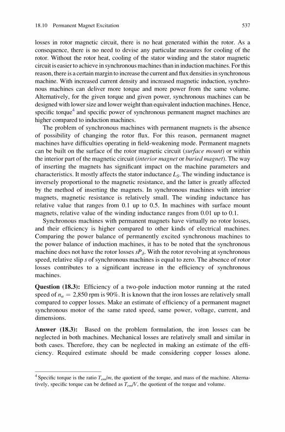
losses in rotor magnetic circuit, there is no heat generated within the rotor. As a
consequence, there is no need to devise any particular measures for cooling of the
rotor. Without the rotor heat, cooling of the stator winding and the stator magnetic
circuit is easier to achieve in synchronousmachines than in inductionmachines. For this
reason, there is a certainmargin to increase the current and fluxdensities in synchronous
machine. With increased current density and increased magnetic induction, synchro-
nous machines can deliver more torque and more power from the same volume.
Alternatively, for the given torque and given power, synchronous machines can be
designedwith lower size and lower weight than equivalent inductionmachines. Hence,
specific torque4 and specific power of synchronous permanent magnet machines are
higher compared to induction machines.
The problem of synchronous machines with permanent magnets is the absence
of possibility of changing the rotor flux. For this reason, permanent magnet
machines have difficulties operating in field-weakening mode. Permanent magnets
can be built on the surface of the rotor magnetic circuit (surface mount) or withinthe interior part of the magnetic circuit (interior magnet or buried magnet). The wayof inserting the magnets has significant impact on the machine parameters and
characteristics. It mostly affects the stator inductance LS. The winding inductance isinversely proportional to the magnetic resistance, and the latter is greatly affected
by the method of inserting the magnets. In synchronous machines with interior
magnets, magnetic resistance is relatively small. The winding inductance has
relative value that ranges from 0.1 up to 0.5. In machines with surface mount
magnets, relative value of the winding inductance ranges from 0.01 up to 0.1.
Synchronous machines with permanent magnets have virtually no rotor losses,
and their efficiency is higher compared to other kinds of electrical machines.
Comparing the power balance of permanently excited synchronous machines to
the power balance of induction machines, it has to be noted that the synchronous
machine does not have the rotor losses sPd. With the rotor revolving at synchronous
speed, relative slip s of synchronous machines is equal to zero. The absence of rotor
losses contributes to a significant increase in the efficiency of synchronous
machines.
Question (18.3): Efficiency of a two-pole induction motor running at the rated
speed of nn ¼ 2,850 rpm is 90%. It is known that the iron losses are relatively small
compared to copper losses. Make an estimate of efficiency of a permanent magnet
synchronous motor of the same rated speed, same power, voltage, current, and
dimensions.
Answer (18.3): Based on the problem formulation, the iron losses can be
neglected in both machines. Mechanical losses are relatively small and similar in
both cases. Therefore, they can be neglected in making an estimate of the effi-
ciency. Required estimate should be made considering copper losses alone.
4 Specific torque is the ratio Tem/m, the quotient of the torque, and mass of the machine. Alterna-
tively, specific torque can be defined as Tem/V, the quotient of the torque and volume.
18.10 Permanent Magnet Excitation 537
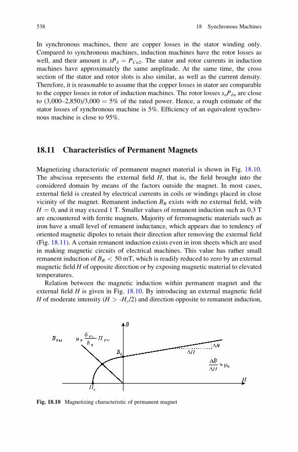
In synchronous machines, there are copper losses in the stator winding only.
Compared to synchronous machines, induction machines have the rotor losses as
well, and their amount is sPd ¼ PCu2. The stator and rotor currents in induction
machines have approximately the same amplitude. At the same time, the cross
section of the stator and rotor slots is also similar, as well as the current density.
Therefore, it is reasonable to assume that the copper losses in stator are comparable
to the copper losses in rotor of induction machines. The rotor losses snPdn are close
to (3,000–2,850)/3,000 ¼ 5% of the rated power. Hence, a rough estimate of the
stator losses of synchronous machine is 5%. Efficiency of an equivalent synchro-
nous machine is close to 95%.
18.11 Characteristics of Permanent Magnets
Magnetizing characteristic of permanent magnet material is shown in Fig. 18.10.
The abscissa represents the external field H, that is, the field brought into the
considered domain by means of the factors outside the magnet. In most cases,
external field is created by electrical currents in coils or windings placed in close
vicinity of the magnet. Remanent induction BR exists with no external field, with
H ¼ 0, and it may exceed 1 T. Smaller values of remanent induction such as 0.3 T
are encountered with ferrite magnets. Majority of ferromagnetic materials such as
iron have a small level of remanent inductance, which appears due to tendency of
oriented magnetic dipoles to retain their direction after removing the external field
(Fig. 18.11). A certain remanent induction exists even in iron sheets which are used
in making magnetic circuits of electrical machines. This value has rather small
remanent induction of BR < 50 mT, which is readily reduced to zero by an external
magnetic field H of opposite direction or by exposing magnetic material to elevated
temperatures.
Relation between the magnetic induction within permanent magnet and the
external field H is given in Fig. 18.10. By introducing an external magnetic field
H of moderate intensity (H > -Hc/2) and direction opposite to remanent induction,
Fig. 18.10 Magnetizing characteristic of permanent magnet
538 18 Synchronous Machines
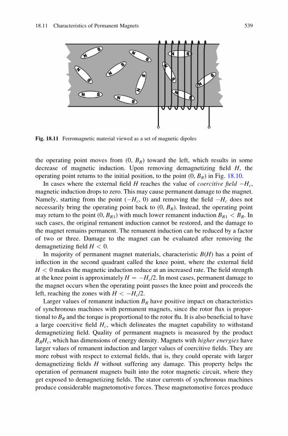
the operating point moves from (0, BR) toward the left, which results in some
decrease of magnetic induction. Upon removing demagnetizing field H, the
operating point returns to the initial position, to the point (0, BR) in Fig. 18.10.
In cases where the external field H reaches the value of coercitive field �Hc,
magnetic induction drops to zero. This may cause permanent damage to the magnet.
Namely, starting from the point (�Hc, 0) and removing the field �Hc does not
necessarily bring the operating point back to (0, BR). Instead, the operating point
may return to the point (0, BR1) with much lower remanent induction BR1 < BR. In
such cases, the original remanent induction cannot be restored, and the damage to
the magnet remains permanent. The remanent induction can be reduced by a factor
of two or three. Damage to the magnet can be evaluated after removing the
demagnetizing field H < 0.
In majority of permanent magnet materials, characteristic B(H) has a point of
inflection in the second quadrant called the knee point, where the external field
H < 0 makes the magnetic induction reduce at an increased rate. The field strength
at the knee point is approximatelyH ¼ �Hc/2. In most cases, permanent damage to
the magnet occurs when the operating point passes the knee point and proceeds the
left, reaching the zones with H < �Hc/2.
Larger values of remanent induction BR have positive impact on characteristics
of synchronous machines with permanent magnets, since the rotor flux is propor-
tional to BR and the torque is proportional to the rotor flu. It is also beneficial to have
a large coercitive field Hc, which delineates the magnet capability to withstand
demagnetizing field. Quality of permanent magnets is measured by the product
BRHc, which has dimensions of energy density. Magnets with higher energies havelarger values of remanent induction and larger values of coercitive fields. They are
more robust with respect to external fields, that is, they could operate with larger
demagnetizing fields H without suffering any damage. This property helps the
operation of permanent magnets built into the rotor magnetic circuit, where they
get exposed to demagnetizing fields. The stator currents of synchronous machines
produce considerable magnetomotive forces. These magnetomotive forces produce
Fig. 18.11 Ferromagnetic material viewed as a set of magnetic dipoles
18.11 Characteristics of Permanent Magnets 539
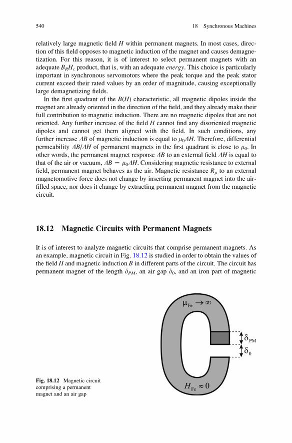
relatively large magnetic field H within permanent magnets. In most cases, direc-
tion of this field opposes to magnetic induction of the magnet and causes demagne-
tization. For this reason, it is of interest to select permanent magnets with an
adequate BRHc product, that is, with an adequate energy. This choice is particularlyimportant in synchronous servomotors where the peak torque and the peak stator
current exceed their rated values by an order of magnitude, causing exceptionally
large demagnetizing fields.
In the first quadrant of the B(H) characteristic, all magnetic dipoles inside the
magnet are already oriented in the direction of the field, and they already make their
full contribution to magnetic induction. There are no magnetic dipoles that are not
oriented. Any further increase of the field H cannot find any disoriented magnetic
dipoles and cannot get them aligned with the field. In such conditions, any
further increase DB of magnetic induction is equal to m0DH. Therefore, differentialpermeability DB/DH of permanent magnets in the first quadrant is close to m0. Inother words, the permanent magnet response DB to an external field DH is equal to
that of the air or vacuum, DB ¼ m0DH. Considering magnetic resistance to external
field, permanent magnet behaves as the air. Magnetic resistance Rm to an external
magnetomotive force does not change by inserting permanent magnet into the air-
filled space, nor does it change by extracting permanent magnet from the magnetic
circuit.
18.12 Magnetic Circuits with Permanent Magnets
It is of interest to analyze magnetic circuits that comprise permanent magnets. As
an example, magnetic circuit in Fig. 18.12 is studied in order to obtain the values of
the field H and magnetic induction B in different parts of the circuit. The circuit has
permanent magnet of the length dPM, an air gap d0, and an iron part of magnetic
Fig. 18.12 Magnetic circuit
comprising a permanent
magnet and an air gap
540 18 Synchronous Machines
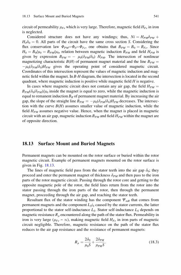
circuit of permeability mFewhich is very large. Therefore, magnetic fieldHFe in iron
is neglected.
Considered structure does not have any windings; thus, Ni ¼ HPMdPM þH0d0 ¼ 0. All parts of the circuit have the same cross section S. Considering the
flux conservation law FPM¼F0¼FFe, one obtains that BPM ¼ B0 ¼ BFe. Since
H0 ¼ B0/m0 ¼ BPM/m0, relation between magnetic induction BPM and field HPM is
given by expression BPM ¼ � m0(dPM/d0) HPM. The intersection of nonlinear
magnetizing characteristic B(H) of permanent magnet material and the line BPM ¼�m0(dPM/d0)HPM gives the operating point of considered magnetic circuit.
Coordinates of this intersection represent the values of magnetic induction and mag-
netic field within the magnet. In B-H diagram, the intersection is located in the second
quadrant, where magnetic induction is positive while magnetic field H is negative.
In cases where magnetic circuit does not contain any air gap, the field HPM ¼BPM(d0/dPM)/m0 inside the magnet is equal to zero, while the magnetic induction is
equal to remanent induction BR of permanent magnet material. By increasing the air
gap, the slope of the straight line BPM ¼ �m0(dPM/d0)HPM decreases. The intersec-
tion with the curve B(H) assumes smaller value of magnetic induction, while the
field HPM assumes negative value. Hence, when the magnet is placed in magnetic
circuit with an air gap, magnetic induction BPM and field HPMwithin the magnet are
of opposite direction.
18.13 Surface Mount and Buried Magnets
Permanent magnets can be mounted on the rotor surface or buried within the rotor
magnetic circuit. Example of permanent magnets mounted on the rotor surface is
given in Fig. 18.13.
The lines of magnetic field pass from the stator teeth into the air gap d0; theyproceed and enter the permanent magnet of thickness dPM and then pass to the iron
parts of the rotor magnetic circuit. Passing through the rotor core and getting to the
opposite magnetic pole of the rotor, the field lines return from the rotor into the
stator passing through the iron parts of the rotor, then through the permanent
magnet, proceeding through the air gap, and reaching the stator teeth.
Resultant flux of the stator winding has the component CmR that comes from
permanent magnets and the component LSiS caused by the stator currents, the latter
proportional to the stator self-inductance LS. Stator self-inductance LS depends onmagnetic resistance Rm encountered along the path of the stator flux. Permeability in
iron is very large (mFe ~ /), making magnetic field HFe in iron parts of magnetic
circuit negligible. Therefore, magnetic resistance on the path of the stator flux
reduces to the air gap resistance and the resistance of permanent magnets:
Rm ¼ 2d0m0S
þ 2dPMmPMS
: (18.3)
18.13 Surface Mount and Buried Magnets 541
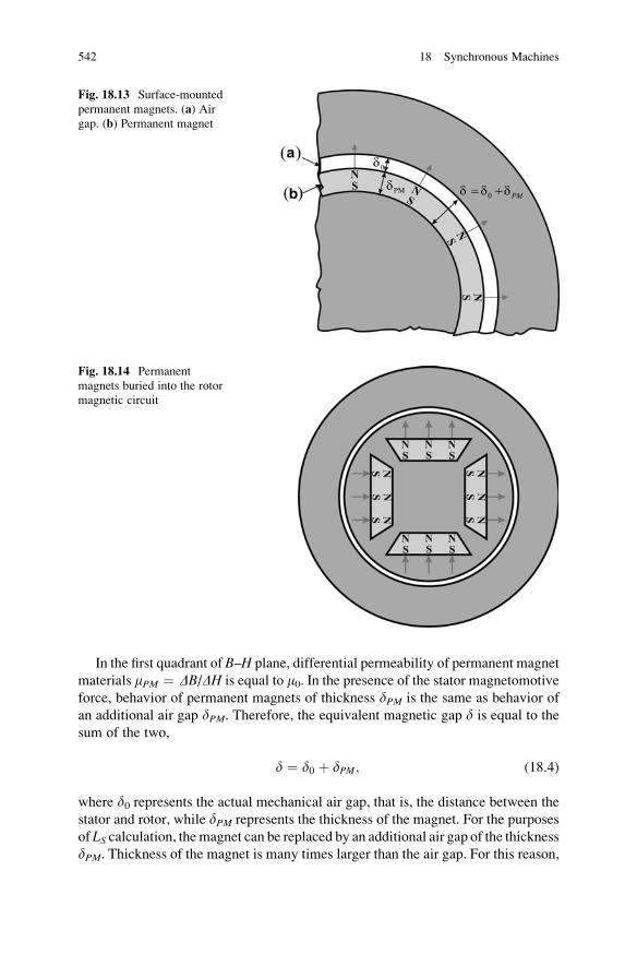
In the first quadrant of B–H plane, differential permeability of permanent magnet
materials mPM ¼ DB/DH is equal to m0. In the presence of the stator magnetomotive
force, behavior of permanent magnets of thickness dPM is the same as behavior of
an additional air gap dPM. Therefore, the equivalent magnetic gap d is equal to the
sum of the two,
d ¼ d0 þ dPM; (18.4)
where d0 represents the actual mechanical air gap, that is, the distance between the
stator and rotor, while dPM represents the thickness of the magnet. For the purposes
of LS calculation, themagnet can be replaced by an additional air gap of the thickness
dPM. Thickness of the magnet is many times larger than the air gap. For this reason,
Fig. 18.13 Surface-mounted
permanent magnets. (a) Air
gap. (b) Permanent magnet
Fig. 18.14 Permanent
magnets buried into the rotor
magnetic circuit
542 18 Synchronous Machines
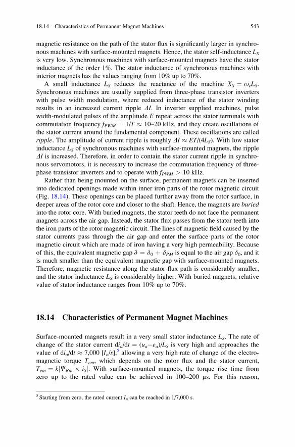
magnetic resistance on the path of the stator flux is significantly larger in synchro-
nous machines with surface-mounted magnets. Hence, the stator self-inductance LSis very low. Synchronous machines with surface-mounted magnets have the stator
inductance of the order 1%. The stator inductance of synchronous machines with
interior magnets has the values ranging from 10% up to 70%.
A small inductance LS reduces the reactance of the machine XS ¼ oeLS.Synchronous machines are usually supplied from three-phase transistor inverters
with pulse width modulation, where reduced inductance of the stator winding
results in an increased current ripple DI. In inverter supplied machines, pulse
width-modulated pulses of the amplitude E repeat across the stator terminals with
commutation frequency fPWM ¼ 1/T � 10–20 kHz, and they create oscillations of
the stator current around the fundamental component. These oscillations are called
ripple. The amplitude of current ripple is roughly DI � ET/(4LS). With low stator
inductance LS of synchronous machines with surface-mounted magnets, the ripple
DI is increased. Therefore, in order to contain the stator current ripple in synchro-
nous servomotors, it is necessary to increase the commutation frequency of three-
phase transistor inverters and to operate with fPWM > 10 kHz.
Rather than being mounted on the surface, permanent magnets can be inserted
into dedicated openings made within inner iron parts of the rotor magnetic circuit
(Fig. 18.14). These openings can be placed further away from the rotor surface, in
deeper areas of the rotor core and closer to the shaft. Hence, the magnets are buriedinto the rotor core. With buried magnets, the stator teeth do not face the permanent
magnets across the air gap. Instead, the stator flux passes from the stator teeth into
the iron parts of the rotor magnetic circuit. The lines of magnetic field caused by the
stator currents pass through the air gap and enter the surface parts of the rotor
magnetic circuit which are made of iron having a very high permeability. Because
of this, the equivalent magnetic gap d ¼ d0 þ dPM is equal to the air gap d0, and it
is much smaller than the equivalent magnetic gap with surface-mounted magnets.
Therefore, magnetic resistance along the stator flux path is considerably smaller,
and the stator inductance LS is considerably higher. With buried magnets, relative
value of stator inductance ranges from 10% up to 70%.
18.14 Characteristics of Permanent Magnet Machines
Surface-mounted magnets result in a very small stator inductance LS. The rate of
change of the stator current dia/dt ¼ (ua�ea)/LS is very high and approaches the
value of dia/dt � 7,000 [In/s],5 allowing a very high rate of change of the electro-
magnetic torque Tem, which depends on the rotor flux and the stator current,
Tem ¼ kjCRm � iSj. With surface-mounted magnets, the torque rise time from
zero up to the rated value can be achieved in 100–200 ms. For this reason,
5 Starting from zero, the rated current In can be reached in 1/7,000 s.
18.14 Characteristics of Permanent Magnet Machines 543
synchronous motors with surface-mounted magnets are used in motion control
applications such as the industry automation and robotics, where the closed loop
speed and position control depend on the ability to effectuate very fast torque
changes.
One shortcoming of synchronous machines with surface-mounted magnets is
their limited ability to operate in the field-weakening region, where the rotor speed
exceeds the rated speed, increasing as well the electromotive force joeCS induced
in the stator windings. Above the rated speed, the stator fluxCS has to be reduced in
order to maintain the electromotive force joeCS within the rated limits, jjoeCSj �Un ¼ Cnon. To this aim, the fluxCS ¼ CRm þ LSiS should be decreased accordingto the law CS(oe) ¼ Cn(on/oe). The flux CRm of permanent magnets cannot
be altered, and the flux reduction requires a demagnetizing component of the stator
current iS. The amount of demagnetizing stator current depends on the
stator inductance. For machines with very small inductance LS ~ 1%, very high
stator currents are required in order to reduce the flux. Therefore, the operation of
synchronous machines with surface-mounted magnets in the zone of flux weaken-
ing is not feasible. Hence, synchronous machines with surface-mounted magnets
are used in motion control applications that require high peak torque capability, fast
torque changes, and low inertia.
There are applications of synchronous machines that do not require fast torque
changes, but they do require the field-weakening operation. In such cases, synchro-
nous machines are used with permanent magnets built into interior6 parts of the
rotor magnetic circuit. With stator teeth facing the iron parts of the rotor magnetic
circuit, magnetic resistance is decreased while the stator self-inductance is
increased. With elevated LS, reduction of the stator flux CS ¼ CRm þ LSiS can be
performed with relatively low stator currents. In absence of losses in the rotor,
synchronous machines with buried magnets are applied in all cases where the
efficiency is of particular importance. Some of these examples are renewable
energy sources and autonomous electrical vehicles.
6 Synchronous machines with permanent magnets that are not placed on the rotor surface, and do
not face the air gap, but reside instead in dedicated holes and chambers carved within inner regions
of the rotor magnetic circuits, located further away from the surface and closer to the shaft are
called buried magnet or interior magnet machines.
544 18 Synchronous Machines
Chapter 19
Mathematical Model of Synchronous Machine
This chapter introduces and explains mathematical model of synchronous
machines. The model considers three-phase synchronous machines with excita-
tion windings or permanent magnets on the rotor. This model does not include
damper windings, which are introduced and explained in Chap. 21. The model
represents transient and steady state behavior in electrical and mechanical
subsystems of synchronous machines. Analysis and discussion introduce and
explain Clarke and Park coordinate transforms. The model includes differential
equations that express the voltage balance in stator and rotor windings, inductance
matrix which relates flux linkages and currents, Newton differential equation of
motion, expression for the air gap power, and expression for the electromagnetic
torque. The model development process is very similar to that of the induction
machine, which is detailed in Chap. 15. Therefore, some considerations are
shortened or removed. The model obtained in this chapter is suitable for both
isotropic (cylindrical) and anisotropic (salient pole) machines. This chapter
closes with some basic considerations on the reluctant torque and synchronous
reluctance machines.
19.1 Modeling Synchronous Machines
Dealing with synchronous generators and synchronous motors requires some basic
knowledge on their electrical and mechanical properties. Electrical properties of
machines involve steady state and transient relations between the machine voltages,
currents, and flux linkages. Mechanical properties have to do with the rotor speed,
electromagnetic torque, and motion resistances. For the purpose of designing the
power supply and controls, it is required to know the equations and expressions that
relate voltages and currents of synchronous machine. Steady state analysis relies on
S.N. Vukosavic, Electrical Machines, Power Electronics and Power Systems,
DOI 10.1007/978-1-4614-0400-2_19, # Springer Science+Business Media New York 2013
545
equivalent circuits that involve the machine parameters and phasors representing
the relevant currents, voltages, and fluxes. Mechanical properties of synchronous
machines are required to design and specify the interface to mechanical loads or
driving turbines.
High-power synchronous machines are used as generators in electrical power
plants. They are connected to three-phase network of constant frequency of f ¼ 50
Hz or f ¼ 60 Hz. Mechanical work is obtained via shaft from a steam or water
turbine; it is converted into electrical energy and supplied to the network. Most
synchronous generators have wound rotors. The excitation winding offers the
possibility of changing the excitation flux by varying the excitation current.
Changes in excitation flux affect the electromotive forces and stator voltages.
This opens the possibility of controlling the voltage of the network and to change
the reactive power. Synchronous machines of lower power are used in applications
such as motion control, vehicle propulsion, industrial robots, and automated pro-
duction machines. In these applications, synchronous machines act as motors. Their
tasks include overcoming the motion resistances, driving the work machines, and
controlling the speed and position of tools and work pieces. There is a tendency of
designing and manufacturing medium- and low-power synchronous machines with
constant excitation based on permanent magnets.
During transients, processes that take place in synchronous motors and
generators, voltages, and currents are related by differential equations describing
the voltage balance in the windings. The voltage balance equations describe the
electrical subsystem of the machine. The mechanical subsystem is described by
Newton differential equation of motion. The set of differential equations and
expressions describing behavior of a synchronous machine is called mathematicalmodel or dynamic model. In what follows, the mathematical model of synchronous
machine is determined, with the aim of establishing the mechanical characteristic
and the steady state equivalent circuit:
• Mechanical characteristic of synchronous machine is dependence of the electro-
magnetic torque on the rotor speed in steady state for given frequency and
amplitude of the stator voltage.
• Steady state equivalent circuit is a network of resistances and inductances which
serves for calculation of electrical currents and flux linkages of synchronous
machine.
In the course of modeling, several approximations are taken, and certain phe-
nomena of secondary importance are neglected. The iron losses are considered as
negligible, and all ferromagnetic materials are assumed to be linear and free from
saturation phenomena. Moreover, all the parasitic capacitances are neglected as
distributed parameter effects. The model of synchronous machine will have:
• N differential equations expressing the voltage balance in windings
• Inductance matrix
• Expression for the torque
• Newton equation of motion
546 19 Mathematical Model of Synchronous Machine
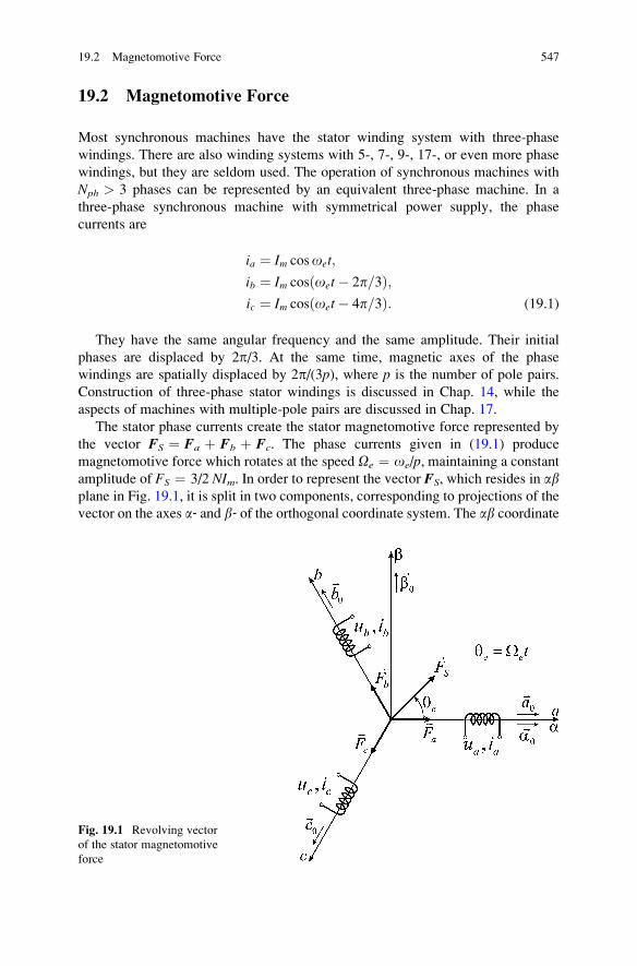
19.2 Magnetomotive Force
Most synchronous machines have the stator winding system with three-phase
windings. There are also winding systems with 5-, 7-, 9-, 17-, or even more phase
windings, but they are seldom used. The operation of synchronous machines with
Nph > 3 phases can be represented by an equivalent three-phase machine. In a
three-phase synchronous machine with symmetrical power supply, the phase
currents are
ia ¼ Im cosoet;
ib ¼ Im cosðoet� 2p=3Þ;ic ¼ Im cosðoet� 4p=3Þ: (19.1)
They have the same angular frequency and the same amplitude. Their initial
phases are displaced by 2p/3. At the same time, magnetic axes of the phase
windings are spatially displaced by 2p/(3p), where p is the number of pole pairs.
Construction of three-phase stator windings is discussed in Chap. 14, while the
aspects of machines with multiple-pole pairs are discussed in Chap. 17.
The stator phase currents create the stator magnetomotive force represented by
the vector FS ¼ Fa þ Fb þ Fc. The phase currents given in (19.1) produce
magnetomotive force which rotates at the speed Oe ¼ oe/p, maintaining a constant
amplitude of FS ¼ 3/2 NIm. In order to represent the vector FS, which resides in abplane in Fig. 19.1, it is split in two components, corresponding to projections of the
vector on the axes a‐ and b‐ of the orthogonal coordinate system. The ab coordinate
Fig. 19.1 Revolving vector
of the stator magnetomotive
force
19.2 Magnetomotive Force 547
system is positioned in such a way that the axis a coincides with the axis of the
phase winding a. Directions of a– and b– axes are defined by unit vectors a0 and b0.
Direction of axes of the phase windings a, b, and c can be expressed in terms of
these unit vectors, a0 ¼ a0, b0 ¼ �½ a0þ b0 sqrt(3)/2, and c0 ¼ �½ a0 � b0 sqrt
(3)/2. Magnetomotive forces of individual phases are
~Fa ¼ Nia~a0;
~Fb ¼ Nib � 1
2~a0 þ
ffiffiffi3
p
2~b0
� �;
~Fc ¼ Nic � 1
2~a0 �
ffiffiffi3
p
2~b0
� �; (19.2)
and the resultant magnetomotive force is equal to
~Fs ¼ ~Fa þ ~Fb þ ~Fc ¼ 3
2NIm ~a0 cosoetþ~b0 sinoet
h i(19.3)
The phase currents in a three-phase winding are not independent variables, and
this makes the modeling more difficult. For star-connected phase windings, the
phase currents are related by ia þ ib þ ic ¼ 0. Similar difficulty exist in delta-
connected phase windings, where ua þ ub þ uc ¼ 0. With ic ¼ �ia �ib, there areonly two independent currents in voltage balance equations. Therefore, it is neces-
sary to replace ic by (�ia � ib) in voltage balance equations for phase c. In addition,the angle between magnetic axes of the phase windings is 2p/3. For windings withspatial displacement of p/2, their mutual inductance is equal to zero. With displace-
ment of 2p/3, there is a nonzero mutual inductances between all the phases, and this
contributes to more complex voltage balance equations. The above shortcomings
can be avoided by introducing the two-phase equivalent of the three-phase machine.
The two-phase equivalent machine can be made with one-phase winding oriented in
direction of unit vector a0 and the other-phase winding oriented in direction of unit
vector b0. With two independent phase currents ia and ib and with the mutual
inductance between the two orthogonal windings equal to zero, the two-phase
model is readily understood.
19.3 Two-Phase Equivalent
The stator current vector iS is determined by dividing the vector FS by the number
of turns of the stator phase winding. The vector iS can be represented as the sum of
two components which are projections of the vector on the axes of ab orthogonal
coordinate frame. These components are ia and ib, and they can be considered as
548 19 Mathematical Model of Synchronous Machine
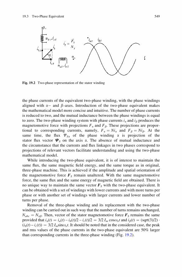
the phase currents of the equivalent two-phase winding, with the phase windings
aligned with a� and b–axes. Introduction of the two-phase equivalent makes
the mathematical model more concise and intuitive. The number of phase currents
is reduced to two, and the mutual inductance between the phase windings is equal
to zero. The two-phase winding system with phase currents ia and ib produces themagnetomotive force with projections Fa and Fb. These projections are propor-
tional to corresponding currents, namely, Fa ¼ Nia and Fb ¼ Nib. At the
same time, the flux CSa of the phase winding a is projection of the
stator flux vector CS on the axis a. The absence of mutual inductance and
the circumstance that the currents and flux linkages in two phases correspond to
projections of relevant vectors facilitate understanding and using the two-phase
mathematical model.
While introducing the two-phase equivalent, it is of interest to maintain the
same flux, the same magnetic field energy, and the same torque as in original,
three-phase machine. This is achieved if the amplitude and spatial orientation of
the magnetomotive force FS remain unaltered. With the same magnetomotive
force, the same flux and the same energy of magnetic field are obtained. There is
no unique way to maintain the same vector FS with the two-phase equivalent. It
can be obtained with a set of windings with lower currents and with more turns per
phase or with another set of windings with larger currents and lower number of
turns per phase.
Removal of the three-phase winding and its replacement with the two-phase
winding can be carried out in such way that the number of turns remains unchanged,
Nabc ¼ Nab. Then, vector of the stator magnetomotive force FS remains the same
provided that ia(t) ¼ ia(t) – ib(t)/2 – ic(t)/2 ¼ 3/2 Im cosoet and ib(t) ¼ (sqrt(3)/2) ·
(ib(t) – ic(t)) ¼ 3/2 Imsinoet. It should be noted that in the considered case, the peakand rms values of the phase currents in the two-phase equivalent are 50% larger
than corresponding currents in the three-phase winding (Fig. 19.2).
Fig. 19.2 Two-phase representation of the stator winding
19.3 Two-Phase Equivalent 549
Starting from previous relations for the phase currents ia and ib, transformation
of the three-phase variables to their two-phase equivalent variables can be written
in the following matrix form:
ia
ib
" #¼ KI
11
2� 1
2
0
ffiffiffi3
p
2�
ffiffiffi3
p
2
2664
3775
ia
ib
ic
264
375 (19.4)
Three-phase to two-phase transform (3F/2F transform) was discussed in Chap. 15.
The following paragraphs are a brief reinstatement of previous considerations.
19.4 Clarke 3F/2F Transform
Three-phase to two-phase transform is known as Clarke transform, named after the
author who proposed the first formulation of the transform. The matrix given in
(19.4) is called transformation matrix. Presence of the adjustable coefficient KI
allows for a certain degree of freedom in defining the two-phase equivalent for the
original three-phase machine. The number of turns of the equivalent machine does
not have to be the same to that of the original machine, provided that the
magnetomotive force remains unaltered. Namely, the condition of invariability of
the magnetomotive force FS can be accomplished by choosing a two-phase equiva-
lent with Nab ¼ mNabc turns. Then, the currents in the phase windings ia(t) and ib(t)should be m times lower in order to maintain the same value of FS. For that reason,
the coefficient KI in (19.4) has to be KI ¼ 1/m. The ratio of the peak currents of thetwo-phase equivalent and the three-phase original is equal to (2/3)/m.
In order to obtain the model of the two-phase machine, it is also necessary to
transform the voltages and fluxes of the original machine to a-b coordinate system.
Clarke transform for the voltages and fluxes is given by the following expressions:
ua
ub
" #¼ KU
11
2� 1
2
0
ffiffiffi3
p
2�
ffiffiffi3
p
2
2664
3775
ua
ub
uc
264
375 (19.5)
Ca
Cb
" #¼ KC
11
2� 1
2
0
ffiffiffi3
p
2�
ffiffiffi3
p
2
2664
3775
Ca
Cb
Cc
264
375 (19.6)
There is possibility to assign different values to coefficients KU, KI, and KC. For
practical reasons, 3F/2F transform is adopted where all the three coefficients are
equal, KU ¼ KI ¼ KC¼K. In this way, the two-phase equivalent maintains the
550 19 Mathematical Model of Synchronous Machine
same ratio of currents, voltages, and fluxes as the original machine, and the 3F/2F transform is invariant in terms of impedances and inductances.1
Question (19.1): Is it possible to actually make a two-phase machine with Nab ¼mNabc turnswhich produces the samemagnetomotive forceFS of the statorwinding as
the original three-phase synchronousmachine andwhich has the voltages and currents
(ua, ub, ia, ib) that are equal to those obtained by applying the Clarke transform to the
voltages and currents of the original machine? It is assumed that transformation
matrices used for the flux, voltage, and current are equal, namely, that they have the
same leading coefficient (KU ¼ KI ¼ KC).
Answer (19.1): The same magnetomotive force FS results in the same flux FS ¼FS/Rm. At the same time, the angular speed of the revolving magnetic field has to be
the same in both 2-phase and 3-phase machines. For that reason, both machines
have the same electromotive force induced in one turn. With that in mind, the phase
voltages of the two-phase equivalent are equal to uab ¼ m uabc. Maintaining the
amplitude of FS requires that the phase currents of the two-phase equivalent are
iab ¼ (3/2)·(iabc/m). Finally, maintaining the ratio of voltages and currents requires
that the ratio uabc/iabc is equal to the ratio uab /iab. Summarizing the above
considerations,
uabiab
¼ muabc3=2ð Þ iabc=mð Þ ¼
2m2
3
uabciabc
¼ uabciabc
) m ¼ffiffiffiffi3
2
r) KU ¼ KI ¼ KC ¼
ffiffiffiffi2
3
r:
� ��
Solution to Question 19.1 proves the possibility to actually make the two-phase
equivalent machine with the same flux, torque, and magnetomotive force and with the
same impedances and inductances as the original machine. The voltages and currents
of the actual two-phase machine are obtained by applying the Clarke transform to the
original variables. Considered two-phase equivalent must have sqrt(3/2) times more
turns than the original machine. Voltages, currents, and fluxes of the two-phase
equivalent are obtained by Clarke transform of the original variables, that is, voltages,
currents, and fluxes of the three-phase winding. The 3F/2F transform to be applied
must have the coefficientsKU ¼ KI ¼ KC¼ sqrt(3/2). The actual two-phasemachine
has the same torque and power as the original machine. Therefore, besides being
impedance-invariant, considered Clarke transform is also power-invariant.2
1 Invariability of impedances and inductances is discussed in Chap. 15. Impedance-invariant
transform results in an equivalent machine where all the impedances are the same as relevant
impedances of the original machine.2 Coordinate transforms do not have to be power-invariant. Generally, coordinate transforms such
as Clarke transform provide another mathematical formulation of the considered dynamic system.
The new model does not have to correspond to any real system. An example to that is the model of
a resistor, u1 ¼ Ri1, obtained by applying the “transform” u1 ¼ 2u, i1 ¼ 2i to the original resistor,described by u ¼ Ri. The model u1 ¼ Ri1 is impedance-invariant, but it is not power-invariant.
19.4 Clarke 3F/2F Transform 551
If the three-phase winding is removed from the magnetic circuit of the original
machine and replaced by the two-phase winding with sqrt(3/2) times more turns,
one obtains a two-phase synchronous machine which replaces the three-phase
machine. The voltages and currents obtained by using 3F/2F transform with
K ¼ sqrt(2/3) are equal to voltages and currents that can be measured on the actual
two-phase machine windings. Hence, considered 3F/2F transform with K ¼ sqrt
(2/3) results in the two-phase equivalent machine that can be actually made. Notice
at this point that the possibility of actually making the machine that comes out of
the 3F/2F transform is not of particular importance.
Clarke transform with K ¼ sqrt(2/3) is invariant in terms of the magnetomotive
force, power, impedance, and inductance. In addition, it can be practically applied
by making a machine with voltages and currents equal to those obtained by the
transform. In spite of that, transform with coefficient K ¼ sqrt(2/3) is seldom used.
The presence of irrational number such as sqrt(2/3) in calculations is the reason for
this particular transform to be rarely used.
In selecting the coordinate transform, there is freedom to choose the coefficient
K so as to facilitate the use of the model. In practice, transforms with KU ¼ KI ¼KC ¼ 2/3 and with KU ¼ KI ¼ KC ¼ 1 are often used. With 3F/2F transform of
currents which uses KI ¼ 1, one obtains the currents ia and ib with peak values and
rms values 50% larger than those of the original variables. Transform which results
in currents ia and ib with peak and rms values equal to those of the phase current ia,ib, and ic, it is required to apply the coefficient K ¼ 2/3. This choice has two
shortcomings.
Clarke transform that uses K ¼ 2/3 is not power-invariant. Namely, the power
calculated in ab domain is not the same as the power of the original machine.
Notice at this point that the rms values of voltages and currents are the same for aband abc variables. The original machine has three-phase windings, while the equi-
valent machine in ab domain has only two-phase windings. Therefore, calculated
power is not the same since Pab ¼ (2/3)Pabc. As a consequence, whenever using the
3F/2F transform with K ¼ 2/3, the actual power of the original machine has to be
calculated on the basis of the expression Pabc ¼ (3/2) Pab.
It is not possible to make an actual two-phase machine that would have the same
voltages and currents as those calculated by the transform. In other words, it is not
possible to rewind the existing three-phase machine and make an equivalent two-
phase machine with voltages and currents that correspond to the values obtained by
the considered 3F/2F transform. On the other hand, the choice K ¼ 2/3 results in
transformed voltages and currents in ab domain that have the same amplitude and
the same rms value as those of voltages and currents of the original three-phase
machine. With K ¼ 2/3, the virtual two-phase equivalent must have a larger
number of turns. In order to maintain the amplitude of the vector FS, it is necessary
to have Nab ¼ (3/2)Nabc. With the same flux per turn F ¼ FS/Rm, the turn
electromotive forces are the same in both the original and the equivalent machine.
Hence, in an attempt to make an actual two-phase equivalent, the two-phase
machine has to be made with the same electromotive force per turn and with 50%
more turns than the original machine. With Nab ¼ (3/2)Nabc, the phase voltages of
552 19 Mathematical Model of Synchronous Machine
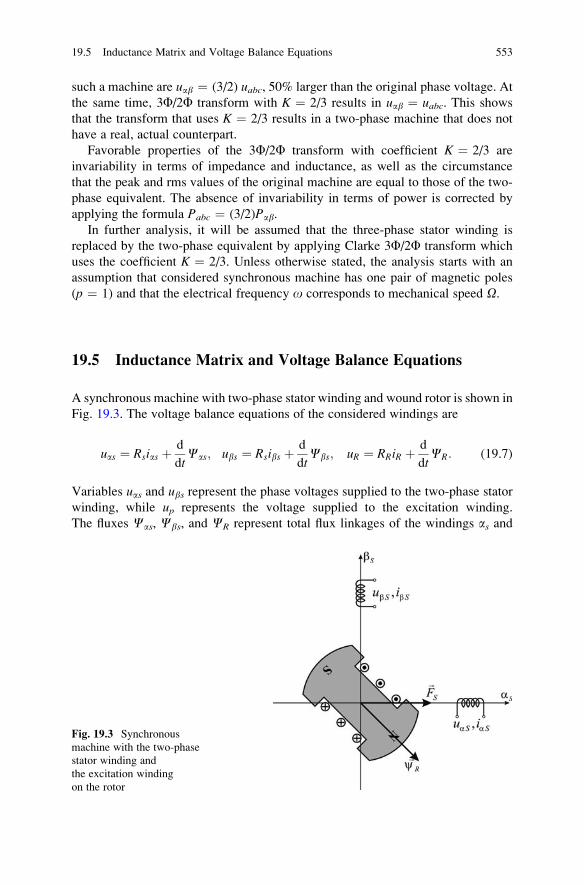
such a machine are uab ¼ (3/2) uabc, 50% larger than the original phase voltage. At
the same time, 3F/2F transform with K ¼ 2/3 results in uab ¼ uabc. This showsthat the transform that uses K ¼ 2/3 results in a two-phase machine that does not
have a real, actual counterpart.
Favorable properties of the 3F/2F transform with coefficient K ¼ 2/3 are
invariability in terms of impedance and inductance, as well as the circumstance
that the peak and rms values of the original machine are equal to those of the two-
phase equivalent. The absence of invariability in terms of power is corrected by
applying the formula Pabc ¼ (3/2)Pab.
In further analysis, it will be assumed that the three-phase stator winding is
replaced by the two-phase equivalent by applying Clarke 3F/2F transform which
uses the coefficient K ¼ 2/3. Unless otherwise stated, the analysis starts with an
assumption that considered synchronous machine has one pair of magnetic poles
(p ¼ 1) and that the electrical frequency o corresponds to mechanical speed O.
19.5 Inductance Matrix and Voltage Balance Equations
A synchronous machine with two-phase stator winding and wound rotor is shown in
Fig. 19.3. The voltage balance equations of the considered windings are
uas ¼ Rsias þ d
dtCas; ubs ¼ Rsibs þ d
dtCbs; uR ¼ RRiR þ d
dtCR: (19.7)
Variables uas and ubs represent the phase voltages supplied to the two-phase stator
winding, while up represents the voltage supplied to the excitation winding.
The fluxes Cas, Cbs, and CR represent total flux linkages of the windings as and
Fig. 19.3 Synchronous
machine with the two-phase
stator winding and
the excitation winding
on the rotor
19.5 Inductance Matrix and Voltage Balance Equations 553
bs and of the excitation winding. Relation between currents ias, ibs, and iR and flux
linkages is given by the inductance matrix. Since the rotor is in motion, the angular
displacement of the excitation winding magnetic axis with respect to as axis of thestator is ym ¼ Omt, assuming that the rotor speedOm does not change. With variable
ym, mutual inductances of the inductance matrix are variable, and the inductance
matrix is a nonstationary matrix:
Cas
Cbs
CR
24
35 ¼
Ls 0 Lm cos ym0 Ls Lm sin ym
Lm cos ym Lm sin ym LR
24
35 �
iasibsiR
24
35 (19.8)
The flux in phase a of the stator winding is equal toCas ¼ LSias þ Lm cos(ym) iR.Variable mutual inductances result in the voltage balance equations that have
trigonometric functions such as cos(ym), where the state variable ym appears as
the function argument. This causes difficulties in deriving a legible steady state
equivalent scheme:
uas ¼ Rsias þ d
dtLSias þ Lm cos ymð ÞiRð Þ
¼ Rsias þ LSd
dtias þ Lm cos ymð Þ d
dtiR � omLmiR sin ymð Þ:
In addition, considered model has the state variables such as the phase currents
ias and ibs which have sinusoidal change even in the steady state. Therefore, their
time derivatives assume nonzero values in steady state conditions, and this creates
difficulties in the steady state analysis and hinders formulation of controls of the
machine. The above mentioned shortcomings are removed by applying Park coor-
dinate transform. This transform represents the machine vectors in revolving dqcoordinate frame. Its application to synchronous machines is very much the same as
the application of Park transform to induction machines, discussed in Chap. 15.
19.6 Park Transform
The model of synchronous machine in stationary aS–bS coordinate frame has two
significant drawbacks which make its use more difficult and hinder the analysis,
conclusion making, and formulation of the control law. These drawbacks are the
following:
• Differential equations expressing the voltage balance comprise trigonometric
functions of state variables. This affects usability of the model and results in
impractical steady state equivalent circuits. Variable coefficients in voltage
balance equations appear due to changes in mutual inductances, which make
elements of the inductance matrix. These changes take place due to variation in
554 19 Mathematical Model of Synchronous Machine
relative position between the rotor, which carries the excitation winding, and the
stator, which carries the stator phase windings.
• First-time derivatives of state variables have nonzero values even in steady state
conditions. State variables of the machine model which is formulated in station-
ary aS–bS coordinate frame are projections of relevant vectors on aS- and bS-axes. At steady state, the rotor speed, the flux amplitude, the electromagnetic
torque, and the conversion power are all constant. Yet, the stator phase currents,
flux linkages of individual phases, their magnetomotive forces, and
electromotive forces are all AC quantities. They exhibit sinusoidal change
even in steady state, and their first-time derivatives are not equal to zero. This
circumstance makes the analysis of steady state operation more difficult.
The model deficiencies mentioned above are removed by applying transforma-
tion of all the state variables to rotating coordinate system with orthogonal d- andq-axes. This dq coordinate frame revolves at the rotor speed, and it is called
synchronous coordinate frame. In most cases, d‐axis is made collinear with mag-
netic axis of the excitation winding. In permanent magnet machines, d-axis is made
collinear with the rotor flux vector which is produced by permanent magnets.
Transformation of currents, voltages, flux linkages, and magnetomotive forces
into dq coordinate frame is called Park transform, and it has been explained in
detail in Chap. 15.
Park transform can be conceived as a replacement of the existing stator phases aSand bS by imaginary, virtual windings residing in synchronously rotating dqcoordinate frame, positioned in such way that the d-axis coincides with magnetic
axis of the excitation winding. This new coordinate system rotates at the same speed
as the rotor, therefore the name synchronous coordinate frame. The voltages,
currents, and flux linkages of the excitation winding do not need to be transformed,
as they reside already within the target dq coordinate frame. Transformation
procedure and notation used hereafter are the same as the ones used in Chap. 15.
The subsequent paragraphs are reduced to a brief reinstatement of the Park trans-
form, already detailed in Chap. 15.
With ydq ¼ ym, the new dq coordinate system revolves at the same speed as the
rotor flux CR. In steady state conditions, relative position between vectors CR and
FS does not change. Hence, dq frame revolves in synchronism with the vector of the
stator magnetomotive force FS as well. Therefore, in steady state conditions,
projections of both vectors on d- and q-axes are constant. The same conclusion
applies to voltage, current, and stator flux vectors. Hence, Park transform provides a
set of variables in synchronously rotating dq frame that all have constant values in
steady state conditions.
Advantage of placing the d-axis along magnetic axis of the excitation winding is
the circumstance that all of the excitation flux extends along the d-axis. Namely, qcomponent of the excitation flux CR is equal to zero. For the setup in Fig. 19.4,
which includes virtual windings d and q and the excitation winding, mutual
inductance between the virtual phase q and the excitation winding is equal to
zero, which simplifies further considerations. In synchronous machines with
19.6 Park Transform 555
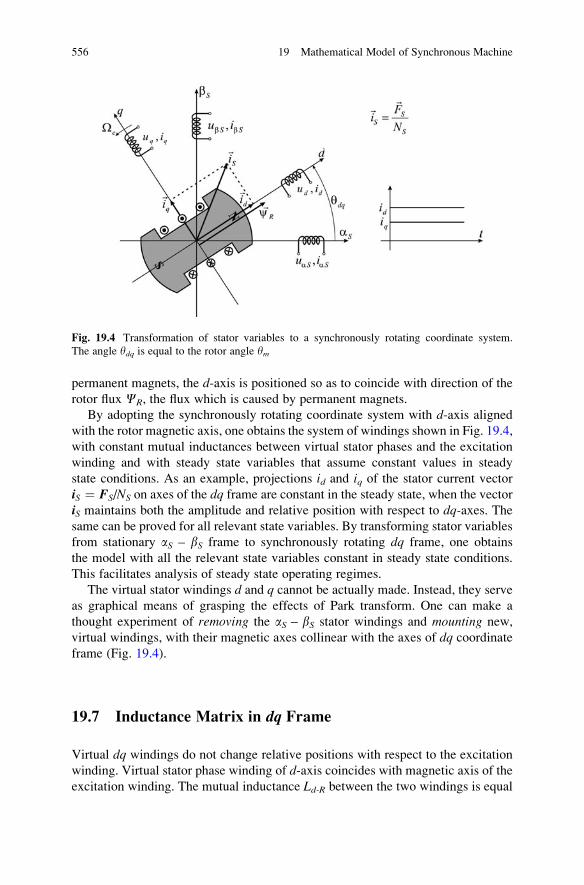
permanent magnets, the d-axis is positioned so as to coincide with direction of the
rotor flux CR, the flux which is caused by permanent magnets.
By adopting the synchronously rotating coordinate system with d-axis alignedwith the rotor magnetic axis, one obtains the system of windings shown in Fig. 19.4,
with constant mutual inductances between virtual stator phases and the excitation
winding and with steady state variables that assume constant values in steady
state conditions. As an example, projections id and iq of the stator current vector
iS ¼ FS/NS on axes of the dq frame are constant in the steady state, when the vector
iS maintains both the amplitude and relative position with respect to dq-axes. Thesame can be proved for all relevant state variables. By transforming stator variables
from stationary aS – bS frame to synchronously rotating dq frame, one obtains
the model with all the relevant state variables constant in steady state conditions.
This facilitates analysis of steady state operating regimes.
The virtual stator windings d and q cannot be actually made. Instead, they serve
as graphical means of grasping the effects of Park transform. One can make a
thought experiment of removing the aS – bS stator windings and mounting new,
virtual windings, with their magnetic axes collinear with the axes of dq coordinate
frame (Fig. 19.4).
19.7 Inductance Matrix in dq Frame
Virtual dq windings do not change relative positions with respect to the excitation
winding. Virtual stator phase winding of d-axis coincides with magnetic axis of the
excitation winding. The mutual inductance Ld-R between the two windings is equal
Fig. 19.4 Transformation of stator variables to a synchronously rotating coordinate system.
The angle ydq is equal to the rotor angle ym
556 19 Mathematical Model of Synchronous Machine
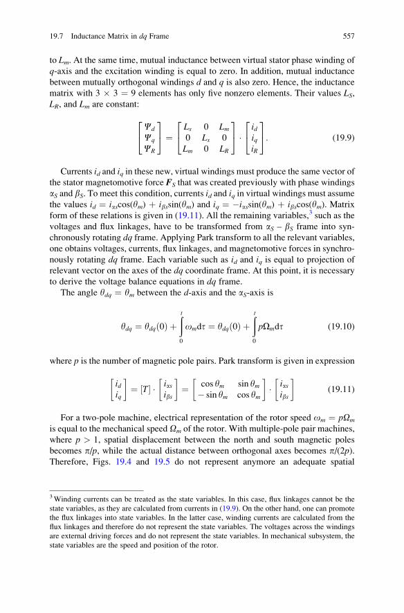
to Lm. At the same time, mutual inductance between virtual stator phase winding of
q-axis and the excitation winding is equal to zero. In addition, mutual inductance
between mutually orthogonal windings d and q is also zero. Hence, the inductance
matrix with 3 � 3 ¼ 9 elements has only five nonzero elements. Their values LS,LR, and Lm are constant:
Cd
Cq
CR
24
35 ¼
Ls 0 Lm0 Ls 0
Lm 0 LR
24
35 �
idiqiR
24
35: (19.9)
Currents id and iq in these new, virtual windings must produce the same vector of
the stator magnetomotive force FS that was created previously with phase windings
aS and bS. To meet this condition, currents id and iq in virtual windings must assume
the values id ¼ iascos(ym) þ ibssin(ym) and iq ¼ �iassin(ym) þ ibscos(ym). Matrix
form of these relations is given in (19.11). All the remaining variables,3 such as the
voltages and flux linkages, have to be transformed from aS – bS frame into syn-
chronously rotating dq frame. Applying Park transform to all the relevant variables,
one obtains voltages, currents, flux linkages, and magnetomotive forces in synchro-
nously rotating dq frame. Each variable such as id and iq is equal to projection of
relevant vector on the axes of the dq coordinate frame. At this point, it is necessary
to derive the voltage balance equations in dq frame.
The angle ydq ¼ ym between the d-axis and the aS-axis is
ydq ¼ ydqð0Þ þðt
0
omdt ¼ ydqð0Þ þðt
0
pOmdt (19.10)
where p is the number of magnetic pole pairs. Park transform is given in expression
idiq
� �¼ T½ � � ias
ibs
� �¼ cos ym sin ym
� sin ym cos ym
� �� ias
ibs
� �(19.11)
For a two-pole machine, electrical representation of the rotor speed om ¼ pOm
is equal to the mechanical speed Om of the rotor. With multiple-pole pair machines,
where p > 1, spatial displacement between the north and south magnetic poles
becomes p/p, while the actual distance between orthogonal axes becomes p/(2p).Therefore, Figs. 19.4 and 19.5 do not represent anymore an adequate spatial
3Winding currents can be treated as the state variables. In this case, flux linkages cannot be the
state variables, as they are calculated from currents in (19.9). On the other hand, one can promote
the flux linkages into state variables. In the latter case, winding currents are calculated from the
flux linkages and therefore do not represent the state variables. The voltages across the windings
are external driving forces and do not represent the state variables. In mechanical subsystem, the
state variables are the speed and position of the rotor.
19.7 Inductance Matrix in dq Frame 557
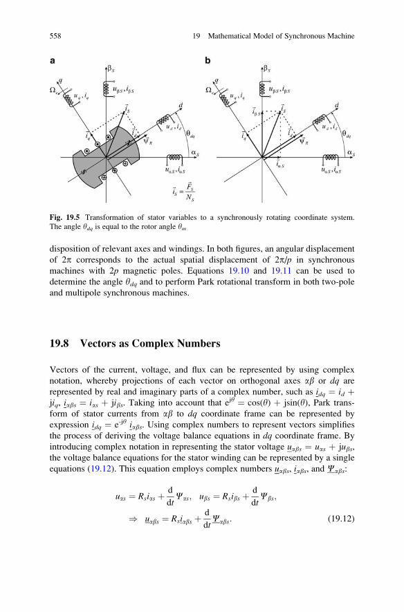
disposition of relevant axes and windings. In both figures, an angular displacement
of 2p corresponds to the actual spatial displacement of 2p/p in synchronous
machines with 2p magnetic poles. Equations 19.10 and 19.11 can be used to
determine the angle ydq and to perform Park rotational transform in both two-pole
and multipole synchronous machines.
19.8 Vectors as Complex Numbers
Vectors of the current, voltage, and flux can be represented by using complex
notation, whereby projections of each vector on orthogonal axes ab or dq are
represented by real and imaginary parts of a complex number, such as idq ¼ id þjiq, iabs ¼ ias þ jibs. Taking into account that ejy ¼ cos(y) þ jsin(y), Park trans-
form of stator currents from ab to dq coordinate frame can be represented by
expression idq ¼ e-jy iabs. Using complex numbers to represent vectors simplifies
the process of deriving the voltage balance equations in dq coordinate frame. By
introducing complex notation in representing the stator voltage uabs ¼ uas þ jubs,the voltage balance equations for the stator winding can be represented by a single
equations (19.12). This equation employs complex numbers uabs, iabs, and Cabs:
uas ¼ Rsias þ d
dtCas; ubs ¼ Rsibs þ d
dtCbs;
) uabs ¼ Rsiabs þd
dtCabs: (19.12)
Fig. 19.5 Transformation of stator variables to a synchronously rotating coordinate system.
The angle ydq is equal to the rotor angle ym
558 19 Mathematical Model of Synchronous Machine
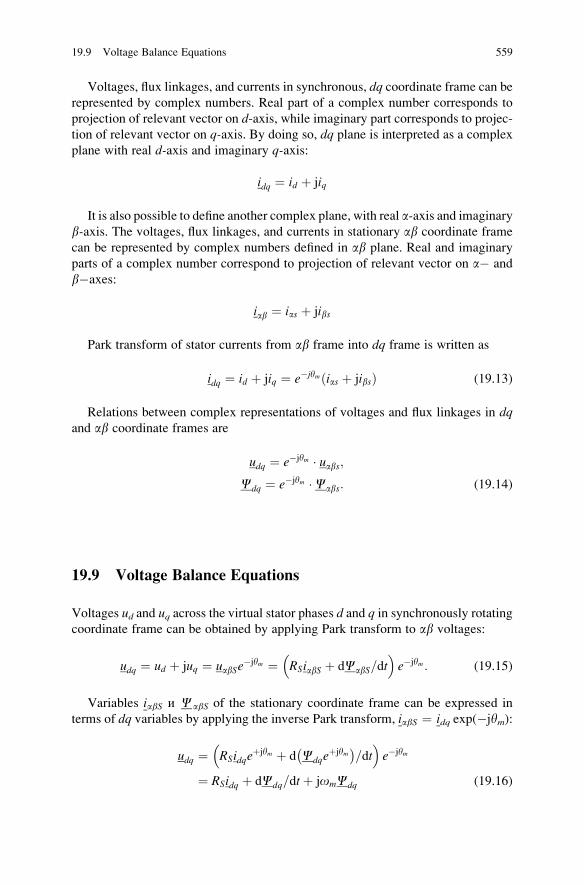
Voltages, flux linkages, and currents in synchronous, dq coordinate frame can be
represented by complex numbers. Real part of a complex number corresponds to
projection of relevant vector on d-axis, while imaginary part corresponds to projec-
tion of relevant vector on q-axis. By doing so, dq plane is interpreted as a complex
plane with real d-axis and imaginary q-axis:
idq ¼ id þ jiq
It is also possible to define another complex plane, with real a-axis and imaginary
b-axis. The voltages, flux linkages, and currents in stationary ab coordinate frame
can be represented by complex numbers defined in ab plane. Real and imaginary
parts of a complex number correspond to projection of relevant vector on a� and
b�axes:
iab ¼ ias þ jibs
Park transform of stator currents from ab frame into dq frame is written as
idq ¼ id þ jiq ¼ e�jymðias þ jibsÞ (19.13)
Relations between complex representations of voltages and flux linkages in dqand ab coordinate frames are
udq ¼ e�jym � uabs;Cdq ¼ e�jym �Cabs: (19.14)
19.9 Voltage Balance Equations
Voltages ud and uq across the virtual stator phases d and q in synchronously rotatingcoordinate frame can be obtained by applying Park transform to ab voltages:
udq ¼ ud þ juq ¼ uabSe�jym ¼ RSiabS þ dCabS=dt
� �e�jym : (19.15)
Variables iabS и CabS of the stationary coordinate frame can be expressed in
terms of dq variables by applying the inverse Park transform, iabS ¼ idq exp(�јym):
udq ¼ RSidqeþjym þ d Cdqe
þjym
=dt� �
e�jym
¼ RSidq þ dCdq=dtþ jomCdq (19.16)
19.9 Voltage Balance Equations 559
whereom ¼ pOm. Therefore, the voltage balance equations in dq frame do not have
the usual form of u ¼ Ri þ dC/dt. They comprise an additional factor which
appears as a consequence of applying rotational transform. Angle ym denotes the
position of magnetic axis of the rotor with respect to the stator phase a. The angularfrequency pOm ¼ om represents the rotor speed. In cases where synchronous
machine has more than one pair of magnetic poles (p > 1), it is necessary to take
into account the circumstance that pOm ¼ om. The angle ym defines the transfor-
mation matrix of Park rotational transform. With p > 1, this angle is p times larger
than the mechanical displacement of the rotor. Starting from the voltage balance
equations in stationary ab coordinate frame
uabs ¼ Rsiabs þd
dtCabs;
one obtains
udq ¼ e�jym Rsiabs þd
dtCabs
� �¼ e�jym Rse
jym idq þd
dtejymCdq
� �� �
Equation which expresses the voltage balance of the stator windings in synchro-
nously rotating dq coordinate system is
udq ¼ Rsidq þd
dtCdq þ jomCdq (19.17)
Equation 19.17 can be split into real and imaginary parts. Each of them
represents a scalar equation
Re udq� � ! ud ¼ Rsid þ d
dtCd � omCq;
Im udq� � ! uq ¼ Rsiq þ d
dtCq þ omCd:
Therefore, the voltage balance equation with complex variables can be split in
two scalar equations:
ud ¼ Rsid þ d
dtCd � omCq;
uq ¼ Rsiq þ d
dtCq þ omCd: (19.18)
The voltage balance equations of the stator windings get affected by Park
transform, and they obtain additional factors such as omCd. At the same time, the
voltage balance equation in excitation winding remains unchanged. This equation
does not get affected by Park transform. Actually, the excitation current, voltage,
560 19 Mathematical Model of Synchronous Machine
and flux linkage do not get transformed by Park transform. Namely, the excitation
winding is fastened to the rotor, and its magnetic axis coincides with d-axis of
synchronously rotating coordinate frame. Thus, transient phenomena of the excita-
tion winding get modeled by the following equation:
uR ¼ RRiR þ d
dtCR (19.19)
19.10 Electrical Subsystem of Isotropic Machines
Mathematical model of synchronous machine describes electrical and mechanicalsubsystem. The former is described by the voltage balance equations and the latter
by Newton equation of motion. With two equivalent phase windings on the stator
and one excitation winding on the rotor, synchronous machine has three windings
and, hence, three differential equations expressing the voltage balance in these
windings. Besides, the model includes the inductance matrix, which provides
relations between flux linkages and currents, as well as the expression for the
electromagnetic torque.
Rotor magnetic circuit of a synchronous machine may be of cylindrical form,
and in this case, magnetic resistance Rm is the same in all directions. Cylindrical
rotor with which maintains the same magnetic resistance in all directions is called
isotropic. Since the self-inductance of each winding depends on the ratio N2/Rm, a
constant magnetic resistance results in constant self-inductances. The stator phase
windings have the same number of turns, and therefore, Ld ¼ Lq ¼ LS. In cases
where magnetic resistances in d- and q-axes are different, the rotor is called
anisotropic. In this case, self-inductances are not the same, Ld 6¼ Lq.Voltage balance equations in (19.8) are written for the windings shown in
Fig. 19.6, and they are applicable to both isotropic and anisotropic synchronous
machines. The difference between the former and the latter appears in the induc-
tance matrix.
Voltage balance equations in virtual stator phase windings in dq coordinate
frame and in the excitation winding are given by
ud ¼ Rsid þ dCd
dt� omCq ;
uq ¼ Rsiq þ dCq
dtþ omCd ;
uR ¼ RRiR þ dCR
dt; (19.20)
19.10 Electrical Subsystem of Isotropic Machines 561
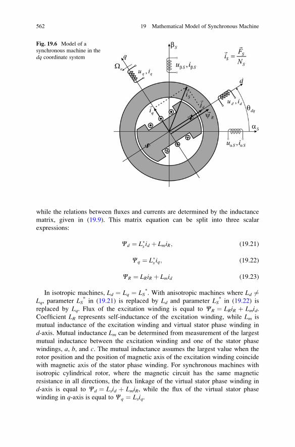
while the relations between fluxes and currents are determined by the inductance
matrix, given in (19.9). This matrix equation can be split into three scalar
expressions:
Cd ¼ L�s id þ LmiR; (19.21)
Cq ¼ L�s iq; (19.22)
CR ¼ LRiR þ Lmid (19.23)
In isotropic machines, Ld ¼ Lq ¼ LS*. With anisotropic machines where Ld 6¼
Lq, parameter LS* in (19.21) is replaced by Ld and parameter LS
* in (19.22) is
replaced by Lq. Flux of the excitation winding is equal to CR ¼ LRiR þ Lmid.Coefficient LR represents self-inductance of the excitation winding, while Lm is
mutual inductance of the excitation winding and virtual stator phase winding in
d-axis. Mutual inductance Lm can be determined from measurement of the largest
mutual inductance between the excitation winding and one of the stator phase
windings, a, b, and c. The mutual inductance assumes the largest value when the
rotor position and the position of magnetic axis of the excitation winding coincide
with magnetic axis of the stator phase winding. For synchronous machines with
isotropic cylindrical rotor, where the magnetic circuit has the same magnetic
resistance in all directions, the flux linkage of the virtual stator phase winding in
d-axis is equal to Cd ¼ Lsid þ LmiR, while the flux of the virtual stator phase
winding in q-axis is equal to Cq ¼ Lsiq.
Fig. 19.6 Model of a
synchronous machine in the
dq coordinate system
562 19 Mathematical Model of Synchronous Machine
19.11 Torque in Isotropic Machines
Electromagnetic torque of an isotropic synchronous machine can be derived by
analyzing the balance of power. It is necessary to consider the electrical power,
delivered to synchronous machine from a three-phase voltage source, mechanical
power on the rotor shaft, and the power of losses in iron, copper, and mechanical
subsystem. Starting from expression for electrical power delivered by the source,
pe ¼ (3/2) (udid þ uqiq), and by using the voltage balance equations for the stator
windings, one obtains the following relation:
pe ¼ 3
2udid þ uqiq
¼ 3
2Rs i2d þ i2q
� �þ 3
2iddCd
dtþ iq
dCq
dt
� �þ 3
2om Cdiq �Cqid
¼ pCu1 þ dWm
dtþ pem: (19.24)
In the above expression, the first factor on the right represents the power of
losses in the stator windings, also called copper losses. There are also iron losses in
stator magnetic circuit, where magnetic inductance B changes with an angular
frequency of om. One of the four approximations taken in modeling electrical
machines is that the iron losses are rather small and therefore negligible
(see Chap. 6, Sect. 6.2). Therefore, considered balance of power does not include
the iron losses. The second factor in the above equation is dWm/dt, and it defines therate of change of the energy accumulated in magnetic coupling field. If the machine
operates with a constant flux, the energy of the magnetic field is constant as well,
and the factor dWm/dt is equal to zero. The third and the last factor of the above
equation is pem ¼ (3/2)om(Cdiq�Cqid). It is obtained by subtracting the losses
from the input electrical power. Therefore, it represents the rate of change of the
electrical energy into mechanical work. It is transferred through the air gap to the
rotor by means of electromagnetic interaction of the stator and rotor fields in the air
gap. The power pem is called power of electromechanical conversion.Synchronous machines have the stator magnetic field revolving in synchronism
with the rotor. In steady state, the angular frequency of the source oe is equal to the
angular frequency of rotation pOm ¼ om. The question arises whether oe ¼ om
during transients. Namely, during transient processes, where the electromagnetic
torque Tem changes, the angle between the stator field FS and the rotor fluxCR may
change as well. The vector FS revolves at the speed oe/p, while the rotor flux CR
revolves at the rotor speed Om. When the angle between the two vectors changes,
there is a temporary difference between oe and pOm ¼ om. When the machine
enters a new steady state, the vectors assume and maintain a new relative position,
and the equation oe ¼ pOm ¼ om is reinstated.
The change between oe and om allows the angle between vectors FS and CR to
change during transients. Yet, they do remain in synchronism, namely, they revolve
19.11 Torque in Isotropic Machines 563
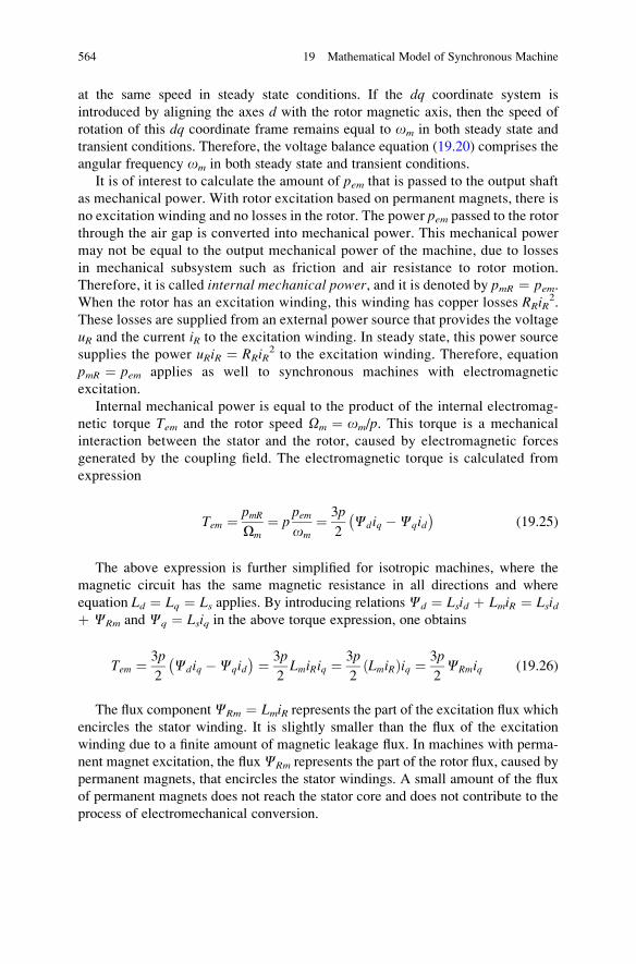
at the same speed in steady state conditions. If the dq coordinate system is
introduced by aligning the axes d with the rotor magnetic axis, then the speed of
rotation of this dq coordinate frame remains equal to om in both steady state and
transient conditions. Therefore, the voltage balance equation (19.20) comprises the
angular frequency om in both steady state and transient conditions.
It is of interest to calculate the amount of pem that is passed to the output shaft
as mechanical power. With rotor excitation based on permanent magnets, there is
no excitation winding and no losses in the rotor. The power pem passed to the rotor
through the air gap is converted into mechanical power. This mechanical power
may not be equal to the output mechanical power of the machine, due to losses
in mechanical subsystem such as friction and air resistance to rotor motion.
Therefore, it is called internal mechanical power, and it is denoted by pmR ¼ pem.When the rotor has an excitation winding, this winding has copper losses RRiR
2.
These losses are supplied from an external power source that provides the voltage
uR and the current iR to the excitation winding. In steady state, this power source
supplies the power uRiR ¼ RRiR2 to the excitation winding. Therefore, equation
pmR ¼ pem applies as well to synchronous machines with electromagnetic
excitation.
Internal mechanical power is equal to the product of the internal electromag-
netic torque Tem and the rotor speed Om ¼ om/p. This torque is a mechanical
interaction between the stator and the rotor, caused by electromagnetic forces
generated by the coupling field. The electromagnetic torque is calculated from
expression
Tem ¼ pmROm
¼ ppemom
¼ 3p
2Cdiq �Cqid
(19.25)
The above expression is further simplified for isotropic machines, where the
magnetic circuit has the same magnetic resistance in all directions and where
equation Ld ¼ Lq ¼ Ls applies. By introducing relations Cd ¼ Lsid þ LmiR ¼ Lsidþ CRm and Cq ¼ Lsiq in the above torque expression, one obtains
Tem ¼ 3p
2Cdiq �Cqid ¼ 3p
2LmiRiq ¼ 3p
2LmiRð Þiq ¼ 3p
2CRmiq (19.26)
The flux componentCRm ¼ LmiR represents the part of the excitation flux whichencircles the stator winding. It is slightly smaller than the flux of the excitation
winding due to a finite amount of magnetic leakage flux. In machines with perma-
nent magnet excitation, the fluxCRm represents the part of the rotor flux, caused by
permanent magnets, that encircles the stator windings. A small amount of the flux
of permanent magnets does not reach the stator core and does not contribute to the
process of electromechanical conversion.
564 19 Mathematical Model of Synchronous Machine
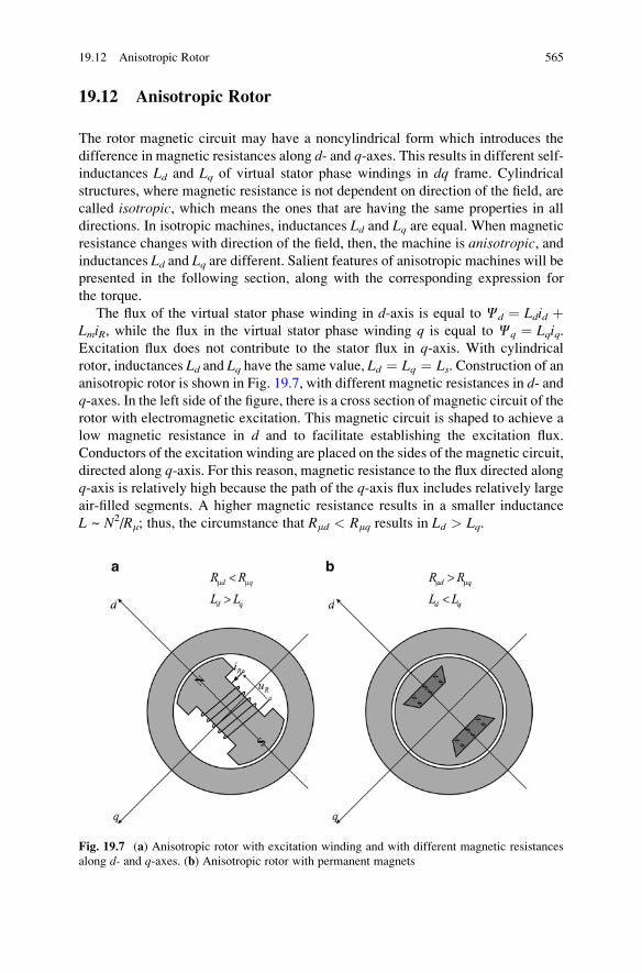
19.12 Anisotropic Rotor
The rotor magnetic circuit may have a noncylindrical form which introduces the
difference in magnetic resistances along d- and q-axes. This results in different self-inductances Ld and Lq of virtual stator phase windings in dq frame. Cylindrical
structures, where magnetic resistance is not dependent on direction of the field, are
called isotropic, which means the ones that are having the same properties in all
directions. In isotropic machines, inductances Ld and Lq are equal. When magnetic
resistance changes with direction of the field, then, the machine is anisotropic, andinductances Ld and Lq are different. Salient features of anisotropic machines will be
presented in the following section, along with the corresponding expression for
the torque.
The flux of the virtual stator phase winding in d-axis is equal to Cd ¼ Ldid þLmiR, while the flux in the virtual stator phase winding q is equal to Cq ¼ Lqiq.Excitation flux does not contribute to the stator flux in q-axis. With cylindrical
rotor, inductances Ld and Lq have the same value, Ld ¼ Lq ¼ Ls. Construction of ananisotropic rotor is shown in Fig. 19.7, with different magnetic resistances in d- andq-axes. In the left side of the figure, there is a cross section of magnetic circuit of the
rotor with electromagnetic excitation. This magnetic circuit is shaped to achieve a
low magnetic resistance in d and to facilitate establishing the excitation flux.
Conductors of the excitation winding are placed on the sides of the magnetic circuit,
directed along q-axis. For this reason, magnetic resistance to the flux directed along
q-axis is relatively high because the path of the q-axis flux includes relatively largeair-filled segments. A higher magnetic resistance results in a smaller inductance
L ~ N2/Rm; thus, the circumstance that Rmd < Rmq results in Ld > Lq.
Fig. 19.7 (a) Anisotropic rotor with excitation winding and with different magnetic resistances
along d- and q-axes. (b) Anisotropic rotor with permanent magnets
19.12 Anisotropic Rotor 565
The second example in Fig. 19.7 shows a rotor magnetic circuit with permanent
magnets built in the interior of the rotor. The magnets are inserted along d-axis.Differential permeability of permanent magnets is close to m0, and their presence onthe flux path in d-axis increases magnetic resistance Rmd. With Rmd > Rmq, the phase
winding inductances are Ld < Lq.Flux linkages of an anisotropic machine are
Cd ¼ Ldid þ LmiR;
Cq ¼ Lqiq;
CR ¼ LRiR þ Lmid: (19.27)
19.13 Reluctant Torque
Differences between self-inductances Ld and Lq of virtual stator phases d and qaffect the expression for the electromagnetic torque:
Tem ¼ 3p
2Cdiq �Cqid
¼ 3p
2CRmiq þ 3p
2Ld � Lq
idiq: (19.28)
The torque expression contains an additional component, proportional to the
difference of self-inductances in d- and q-axes. This torque component is called
reluctant torque because it appears as a consequence of differences in magnetic
resistances, also called reluctances. Reluctant torque may exist even in synchro-
nous machines with no excitation winding and no permanent magnets. It is suffi-
cient to have different magnetic resistances in d- and q-axes and different
inductances Ld and Lq. In the absence of the rotor flux, only the stator field exists
in the air gap. This torque tends to bring the rotor in position where it pays the
minimum magnetic resistance to the stator flux. Hence, it acts toward aligning the
rotor axis of minimum magnetic resistance with the stator flux. There are synchro-
nous machines that are made with no permanent magnets and no excitation
windings. Instead, their rotors have considerable differences of the magnetic
resistances between the direct d-axis and quadrature q-axis. This increases the
difference Ld�Lq and, hence, the reluctant torque. These machines are called
synchronous reluctance machines.
Question (19.2): A synchronous machine has an anisotropic rotor with no perma-
nent magnets and no excitation winding. The amplitude of the stator current is
limited to Im. Determine the largest possible value of the reluctant torque.
All parameters affecting the reluctant torque are known.
566 19 Mathematical Model of Synchronous Machine
Answer (19.2): Reluctant torque is proportional to the product of currents id and iq.When the amplitude of the stator current is limited, the current components can be
expressed as id ¼ Imcos(x) and iq ¼ Imsin(x), where x is the angle between the
stator current vector and d-axis. The reluctant torque is then
Tem ¼ 3p
2Ld � Lq
I2m cos x sin x ¼ 3p
4Ld � Lq
I2m sin 2x:
The highest reluctant torque is obtained for x ¼ p/4, when id ¼ iq ¼ Im/sqrt(2),and it is equal to (3p/4)(Ld � Lq)Im
2.
19.14 Reluctance Motor
Synchronous reluctance machines are used in applications where the size and
weight have no particular importance and where the prevailing goal is to have a
construction which is robust, simple, and low cost. Reluctance machines have no
active parts on the rotor. Rotor has only magnetic circuit made to have different
magnetic resistances in direct and quadrature axes. The rotor magnetic circuit can
be obtained by stacking the iron sheets in the way shown in Fig. 19.8. By stacking
the iron sheets, one obtains a small magnetic resistance along the sheets and a
large magnetic resistance in direction perpendicular to the sheets. The flux that
passes in direction perpendicular to the sheets passes a number of times through
the insulation gaps between the sheets, which increase the equivalent magnetic
resistance. In the prescribed way, one obtains an anisotropic rotor, the rotor with
different magnetic resistances in d- and q-axes. At the same time, the external
appearance of the rotor is cylindrical, with no salient poles and with a low air
drag. Therefore, the rotor may reach high speeds without significant motion
resistances and without jeopardizing mechanical integrity of the machine.
Fig. 19.8 Rotor of a reluctant
synchronous machine
19.14 Reluctance Motor 567
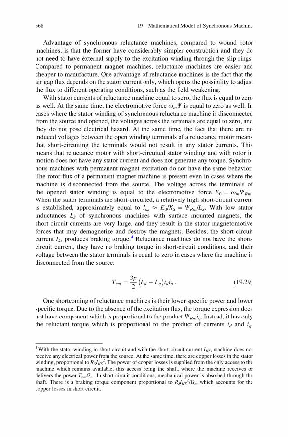
Advantage of synchronous reluctance machines, compared to wound rotor
machines, is that the former have considerably simpler construction and they do
not need to have external supply to the excitation winding through the slip rings.
Compared to permanent magnet machines, reluctance machines are easier and
cheaper to manufacture. One advantage of reluctance machines is the fact that the
air gap flux depends on the stator current only, which opens the possibility to adjust
the flux to different operating conditions, such as the field weakening.
With stator currents of reluctance machine equal to zero, the flux is equal to zero
as well. At the same time, the electromotive force omC is equal to zero as well. In
cases where the stator winding of synchronous reluctance machine is disconnected
from the source and opened, the voltages across the terminals are equal to zero, and
they do not pose electrical hazard. At the same time, the fact that there are no
induced voltages between the open winding terminals of a reluctance motor means
that short-circuiting the terminals would not result in any stator currents. This
means that reluctance motor with short-circuited stator winding and with rotor in
motion does not have any stator current and does not generate any torque. Synchro-
nous machines with permanent magnet excitation do not have the same behavior.
The rotor flux of a permanent magnet machine is present even in cases where the
machine is disconnected from the source. The voltage across the terminals of
the opened stator winding is equal to the electromotive force E0 ¼ omCRm.
When the stator terminals are short-circuited, a relatively high short-circuit current
is established, approximately equal to Iks � E0/XS ¼ CRm/LS. With low stator
inductances LS of synchronous machines with surface mounted magnets, the
short-circuit currents are very large, and they result in the stator magnetomotive
forces that may demagnetize and destroy the magnets. Besides, the short-circuit
current Iks produces braking torque.4 Reluctance machines do not have the short-
circuit current, they have no braking torque in short-circuit conditions, and their
voltage between the stator terminals is equal to zero in cases where the machine is
disconnected from the source:
Tem ¼ 3p
2Ld � Lq
idiq : (19.29)
One shortcoming of reluctance machines is their lower specific power and lower
specific torque. Due to the absence of the excitation flux, the torque expression does
not have component which is proportional to the productCRmiq. Instead, it has onlythe reluctant torque which is proportional to the product of currents id and iq.
4With the stator winding in short circuit and with the short-circuit current IKS, machine does not
receive any electrical power from the source. At the same time, there are copper losses in the stator
winding, proportional to RSIKS2. The power of copper losses is supplied from the only access to the
machine which remains available, this access being the shaft, where the machine receives or
delivers the power TemOm. In short-circuit conditions, mechanical power is absorbed through the
shaft. There is a braking torque component proportional to RSIKS2/Om which accounts for the
copper losses in short circuit.
568 19 Mathematical Model of Synchronous Machine
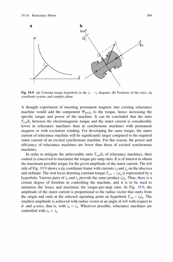
A thought experiment of inserting permanent magnets into existing reluctance
machine would add the component CRmiq to the torque, hence increasing the
specific torque and power of the machine. It can be concluded that the ratio
Tem/IS between the electromagnetic torque and the stator current is considerably
lower in reluctance machines than in synchronous machines with permanent
magnets or with excitation winding. For developing the same torque, the stator
current of reluctance machine will be significantly larger compared to the required
stator current of an excited synchronous machine. For this reason, the power and
efficiency of reluctance machines are lower than those of excited synchronous
machines.
In order to mitigate the unfavorable ratio Tem/IS of reluctance machines, their
control is conceived to maximize the torque-per-amp ratio. It is of interest to obtain
the maximum possible torque for the given amplitude of the stator current. The left
side of Fig. 19.9 shows a dq coordinate frame with currents id and iq on the abscissaand ordinate. The root locus denoting constant torque Tem ~ idiq is represented by ahyperbola. Various pairs of id and iq provide the same product idiq. Thus, there is acertain degree of freedom in controlling the machine, and it is to be used to
minimize the losses and maximize the torque-per-amp ratio. In Fig. 19.9, the
amplitude of the stator current is proportional to the radius vector that starts from
the origin and ends at the selected operating point on hyperbola Tem ~ idiq. Thesmallest amplitude is achieved with radius vector at an angle of p/4 with respect to
d- and q-axes, that is, with id ¼ iq. Wherever possible, reluctance machines are
controlled with id ¼ iq.
Fig. 19.9 (a) Constant torque hyperbola in the id � iq diagram. (b) Positions of the rotor, dqcoordinate system, and complex plane
19.14 Reluctance Motor 569
Chapter 20
Steady-State Operation
Mathematical model of electrical machine contains differential and algebraic
equations describ,ing the machine operation in given supply conditions and given
load. Using the model, it is possible to derive the changes of the rotor speed,
electromagnetic torque, the air-gap flux, and phase currents during transients and
in steady-state conditions. The model is needed to design the power supply of the
machine and to devise control algorithm. At the same time, the model is used to
predict performance of the machine in operating conditions of interest and to
evaluate whether the machine is suitable for given application.
The study of characteristics of synchronous machines and their performance
begins with steady-state analysis. It deals with steady-state operating conditions,
where the machine operates with constant speed, torque, and flux amplitude.
In this chapter, mathematical model is used to derive the steady-state equivalent
circuit of synchronous machine and to obtain the torque and power expressions in
steady-state conditions. Operation at steady state is analyzed and illustrated by
means of phasor diagrams. Some basic notions on phasors are reinstated and
exercised for isotropic and anisotropic machines. The power angle is introduced
and defined, and the steady-state torque is expressed in terms of the power angle.
This chapter discusses and explains electrical and mechanical properties of syn-
chronous machines supplied from stiff three-phase network. Steady-state operation
of synchronous motors and generators is analyzed on the basis of corresponding
phasor diagrams, and the expressions for the torque, active power, and reactive
power are derived in terms of the power angle.
20.1 Voltage Balance Equations at Steady State
Park transform of the state variables has been carried out with the aim of obtaining
the model of a synchronous machine where all the state variables are constant at
steady state. Projections of vectors of the stator current, voltage, and flux on dq axes
S.N. Vukosavic, Electrical Machines, Power Electronics and Power Systems,
DOI 10.1007/978-1-4614-0400-2_20, # Springer Science+Business Media New York 2013
571
of synchronously rotating coordinate frame do not change in steady-state conditions.
Therefore, their first-time derivatives are equal to zero. This facilitates obtaining
the steady-state equivalent scheme. At steady state, the complex numbers udq, idq,andCdq, which represent the vectors of the stator voltage, current, and flux, become
complex constants. Their constant, steady-state values are denoted by us, is, andCs.
These complex constants have their amplitude and angle and therefore may be
treated as phasors. It is important to notice that complex constants us and is representthe steady-state voltages and currents of in three-phase stator winding. Hence, unlike
common phasors, the numbers us and is represent alternating voltages and currents ina three-phase system.
The absolute value of a common phasor corresponds to the rms value of the AC
quantity represented by the phasor. On the other hand, the absolute values of
complex numbers us and is depend on the leading coefficient of Clarke 3F/2F trans-
form. Namely, relation between the rms value of the stator phase voltages and the
absolute value jusj ¼ sqrt(ud2 þ uq
2) of the complex constant us is determined by
coefficient K of 3F/2F transform which is used in deriving the two-phase equiva-
lent of the three-phase machine. With K ¼ 2/3, the absolute value jusj is equal tothe peak value of the stator phase voltages. To facilitate the analysis of synchronous
machines, it is desirable to represent the voltage balance equations by the steady-
state equivalent scheme. At steady state, there is no change of the excitation current
and the excitation flux; thus,
iR ¼ const: ¼ IR
LmIR ¼ CRm:
In synchronous machines with permanent magnets on the rotor, the rotor flux
that encircles the stator winding is constant and equal to CRm. In steady state, the
rotor speed is equal to the synchronous speed; thus, Om ¼ Oe. With angular
frequency oe of the stator voltages and currents, synchronous speed is equal to
Oe ¼ oe/p, and it determines the speed of rotation of the stator magnetic field.
Therefore, Om ¼ Oe ¼ oe/p ¼ om/p. Synchronously rotating dq coordinate frame
is selected so as to have the d‐axis collinear with the excitation flux, that is, with theflux of permanent magnets. Therefore, dq frame revolves at the same speed as the
rotor. Relation between the electrical frequency o and the mechanical speed of
rotation O in multipole machines is o ¼ pO. Hence, the frequency which appears
in voltage balance equations is equal to om ¼ pOm. At steady state, equation
oe ¼ om holds.
For isotropic synchronous machine that operates in the steady state, the voltage
balance equations of the stator windings are given below:
ud ¼ Rsid þ Lsdiddt
� oeLsiq ¼ Rsid � oeLsiq
uq ¼ Rsiq þ Lsdiqdt
þ oeLsid þ oeCRm ¼ Rsiq þ oeLsid þ oeCRm:
572 20 Steady-State Operation
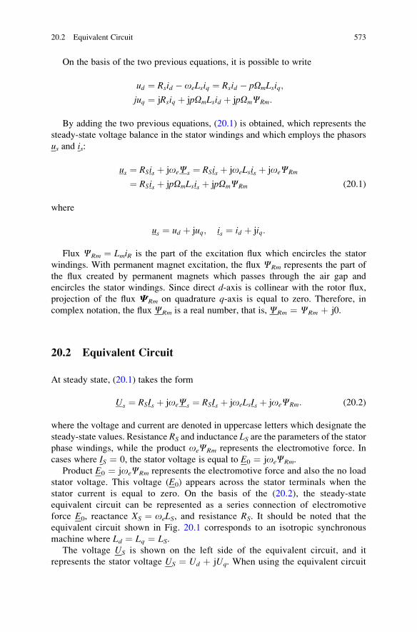
On the basis of the two previous equations, it is possible to write
ud ¼ Rsid � oeLsiq ¼ Rsid � pOmLsiq;
juq ¼ jRsiq þ jpOmLsid þ jpOmCRm:
By adding the two previous equations, (20.1) is obtained, which represents the
steady-state voltage balance in the stator windings and which employs the phasors
us and is:
us ¼ RSis þ joeCs ¼ RSis þ joeLsis þ joeCRm
¼ RSis þ jpOmLsis þ jpOmCRm (20.1)
where
us ¼ ud þ juq; is ¼ id þ jiq:
Flux CRm ¼ LmiR is the part of the excitation flux which encircles the stator
windings. With permanent magnet excitation, the flux CRm represents the part of
the flux created by permanent magnets which passes through the air gap and
encircles the stator windings. Since direct d-axis is collinear with the rotor flux,
projection of the flux CRm on quadrature q-axis is equal to zero. Therefore, in
complex notation, the flux CRm is a real number, that is, CRm ¼ CRm þ j0.
20.2 Equivalent Circuit
At steady state, (20.1) takes the form
Us ¼ RSIs þ joeCs ¼ RSIs þ joeLsIs þ joeCRm: (20.2)
where the voltage and current are denoted in uppercase letters which designate the
steady-state values. Resistance RS and inductance LS are the parameters of the stator
phase windings, while the product oeCRm represents the electromotive force. In
cases where IS ¼ 0, the stator voltage is equal to E0 ¼ joeCRm.
Product E0 ¼ joeCRm represents the electromotive force and also the no load
stator voltage. This voltage (E0) appears across the stator terminals when the
stator current is equal to zero. On the basis of the (20.2), the steady-state
equivalent circuit can be represented as a series connection of electromotive
force E0, reactance XS ¼ oeLS, and resistance RS. It should be noted that the
equivalent circuit shown in Fig. 20.1 corresponds to an isotropic synchronous
machine where Ld ¼ Lq ¼ LS.The voltage US is shown on the left side of the equivalent circuit, and it
represents the stator voltage US ¼ Ud þ jUq. When using the equivalent circuit
20.2 Equivalent Circuit 573
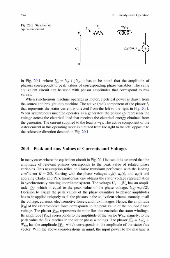
in Fig. 20.1, where US ¼ Ud þ jUq, it has to be noted that the amplitude of
phasors corresponds to peak values of corresponding phase variables. The same
equivalent circuit can be used with phasor amplitudes that correspond to rms
values.
When synchronous machine operates as motor, electrical power is drawn from
the source and brought into machine. The active (real) component of the phasor ISthat represents the stator current is directed from the left to the right in Fig. 20.1.
When synchronous machine operates as a generator, the phasor US represents the
voltage across the electrical load that receives the electrical energy obtained from
the generator. The current supplied to the load is �IS. The active component of the
stator current in this operating mode is directed from the right to the left, opposite to
the reference direction denoted in Fig. 20.1.
20.3 Peak and rms Values of Currents and Voltages
In many cases where the equivalent circuit in Fig. 20.1 is used, it is assumed that the
amplitude of relevant phasors corresponds to the peak value of related phase
variables. This assumption relies on Clarke transform performed with the leading
coefficient K ¼ 2/3. Starting with the phase voltages ua(t), ub(t), and uc(t) and
applying Clarke and Park transforms, one obtains the stator voltage representation
in synchronously rotating coordinate system. The voltage Ud þ jUq has an ampli-
tude jUSj which is equal to the peak value of the phase voltage, Ueff ·sqrt(2).
Decision to assign the peak values of the phase quantities to phasor amplitudes
has to be applied uniquely to all the phasors in the equivalent scheme, namely, to all
the voltage, currents, electromotive forces, and flux linkages. Hence, the amplitude
jE0j of the electromotive force corresponds to the peak value of the no load phase
voltage. The phasorCRm represents the rotor flux that encircles the stator windings.
Its amplitude jCRmj corresponds to the amplitude of the vectorCRm, namely, to the
peak value the flux reaches in the stator phase windings. The phasor CS ¼ LSIS þCRm has the amplitude jCSj which corresponds to the amplitude of the stator flux
vector. With the above considerations in mind, the input power to the machine is
Fig. 20.1 Steady-state
equivalent circuit
574 20 Steady-State Operation
equal to Pe ¼ (3/2) Re(USIS*).1 The power of losses in the stator windings is calcu-
lated as PCu1 ¼ (3/2)RSIS2. The power of electromechanical conversion is equal to
Pem ¼ Pe –PCu1 ¼ (3/2) Re(E0 IS*). Since flux vector CRm coincides with d-axis,
which is assigned to be the real axis of the complex d þ jq plane, the electromotive
force phasor is equal to E0 ¼ joeCRm and it is collinear with quadrature axis (q),which is at the same time the imaginary axis of the complex d þ jq plane. For this
reason, the product E0IS* assumes the value oeCRmIq. The electromagnetic torque is
equal to the ratio of the power Pem and the synchronous speed Oe ¼ oe/p:
Tem ¼ Pem
Oe¼ 3p
2oeoeCRmIq ¼ 3p
2CRmIq : (20.3)
It is also possible to interpret the phasors of the equivalent circuit as complex
numbers with amplitudes that represent rms values of relevant phase variables. In this
case, the equivalent circuit operates with rms voltages and currents. The phasorUS on
the left side of the equivalent circuit represents the stator voltage, and it has an
amplitude jUSj that corresponds to the rms value Urms of the stator phase voltages.
Now, the electromotive force jE0j corresponds to the rms value of the no load phase
voltage. For many, working with rms values of voltages and currents is more handy.
When using the phasors that correspond to rms values, the flux phasors have to be
treated in the same way. Therefore, the phasorCRm, as calculated from the equivalent
circuit, obtains an amplitude which is sqrt(2) times smaller than the amplitude of the
flux vector CRm. At the same time, the value jCSj ¼ jLSIS þ CRmj is equal to the
amplitude of the stator flux vector divided by sqrt(2). Adopting the phasors that
correspond to rms values, the input power to the machine is calculated as Pe ¼ 3 Re
(US IS*); the power of losses in the stator winding is obtained as PCu1 ¼ 3RSIS
2,
while the power of the electromechanical conversion is equal to Pem ¼ Pe –PCu1 ¼3 Re(E0 IS
*) ¼ 3oeCRmIq. Notice at this point that both CRm and Iq in the previous
expression assume the values that are sqrt(2) times smaller than the values in (20.3).
When using phasors that correspond to rms values, the electromagnetic torque is
calculated as
Tem ¼ Pem
Oe¼ 3p
oeoeCRmIq ¼ 3pCRmIq : (20.4)
Question (20.1): A two-pole synchronous machine has the stator self-inductance
LS, while the stator resistance RS is small and it can be neglected. Machine has
permanent magnets on the rotor, and they create the fluxCRm in the stator windings.
Machine operates at steady state, connected to a three-phase network of frequency
fe ¼ 50 Hz, wherein the rms value of phase voltages is USn. The stator voltages
1 Re(z) ¼ zr is the real pert of the complex number z ¼ zr þ jzi. The value z* is equal to
z* ¼ zr � jzi.
20.3 Peak and rms Values of Currents and Voltages 575
have a phase advance d with respect to corresponding no load electromotive forces.
Calculate the power delivered by the network to the machine.
Answer (20.1): The equivalent circuit is analyzed by assuming that the involved
phasors represent the rms values. The stator current of the machine is equal to
IS ¼ (US � E0)/jXS, where E0 ¼ joeCRm. The flux CRm ¼ CRm remains on the
real axis. Since the stator voltages lead with respect to electromotive forces by d,while the electromotive force E0 ¼ joeCRm resides on the imaginary axis, the
stator voltages lead with respect to the real axis by d þ p/2. Components of the
stator voltage in dq frame are Ud ¼ �USnsin(d) and Uq ¼ USncos(d). Therefore,
US ¼ �USn sin dþ jUSn cos d;
IS ¼US � E0
jXS¼ �USn sin dþ jUSn cos d� joeCRm
jXS
¼ USn cos d� oeCRm
XSþ j
USn sin dXS
:
Electrical power received from the network is calculated from the following
expression:
S ¼ 3USI�S ¼ 3
USn oeCRmð ÞXS
sin dð Þ þ j3USn USn � oeCRm cos dð Þð Þ
XS¼ Pe þ jQe:
The active power received by the machine is Pe ¼ 3USn E0 sin(d)/XS.
20.4 Phasor Diagram of Isotropic Machine
Analysis of steady states based on the equivalent circuit relies on complex notation
where the vectors of the stator voltages, currents, and flux linkages are represented by
corresponding phasors. The voltage balance in the steady-state equivalent circuit can
be represented by phasor diagram. The phasor diagram in Fig. 20.2 represents the
balance of voltages in isotropic synchronous machine that operates in motoringmode.
d-Axis of synchronously rotating coordinate frame is assigned as the real axis of the
complex plane.2 Thus, the q-axis becomes imaginary axis. Park rotational transform is
2 Steady-state voltages and currents can be represented as phasors in an arbitrary complex plane.
The angle between the phasor and the real axis determines the initial phase of considered AC
voltages and currents. Apparently, this imposes a constraint on the choice of the position of the real
axis. On the other hand, the initial phase is the value of the phase at the instant t ¼ 0. Therefore, by
choosing the instant t ¼ 0, it is possible to select complex planes with different position of their
real and imaginary axes. Phasor diagrams of synchronous machines are mostly drawn in the
complex plane where the real axis coincides with d-axis of synchronously rotating coordinate
system. It is also of interest to notice that other choices are legitimate as well. When solving some
problems, the calculations are more simple when the real axis is selected to be aligned with the
stator voltage or the stator current.
576 20 Steady-State Operation
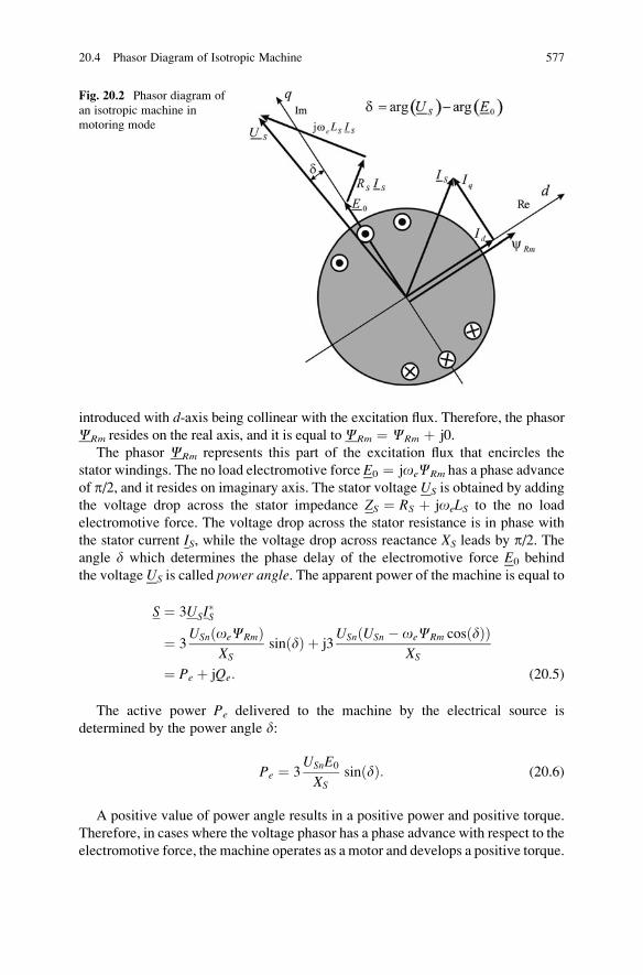
introduced with d-axis being collinear with the excitation flux. Therefore, the phasorCRm resides on the real axis, and it is equal toCRm ¼ CRm þ j0.
The phasor CRm represents this part of the excitation flux that encircles the
stator windings. The no load electromotive force E0 ¼ joeCRm has a phase advance
of p/2, and it resides on imaginary axis. The stator voltage US is obtained by adding
the voltage drop across the stator impedance ZS ¼ RS þ joeLS to the no load
electromotive force. The voltage drop across the stator resistance is in phase with
the stator current IS, while the voltage drop across reactance XS leads by p/2. Theangle d which determines the phase delay of the electromotive force E0 behind
the voltage US is called power angle. The apparent power of the machine is equal to
S ¼ 3USI�S
¼ 3USn oeCRmð Þ
XSsin dð Þ þ j3
USn USn � oeCRm cos dð Þð ÞXS
¼ Pe þ jQe: (20.5)
The active power Pe delivered to the machine by the electrical source is
determined by the power angle d:
Pe ¼ 3USnE0
XSsin dð Þ: (20.6)
A positive value of power angle results in a positive power and positive torque.
Therefore, in cases where the voltage phasor has a phase advance with respect to the
electromotive force, the machine operates as a motor and develops a positive torque.
Fig. 20.2 Phasor diagram of
an isotropic machine in
motoring mode
20.4 Phasor Diagram of Isotropic Machine 577
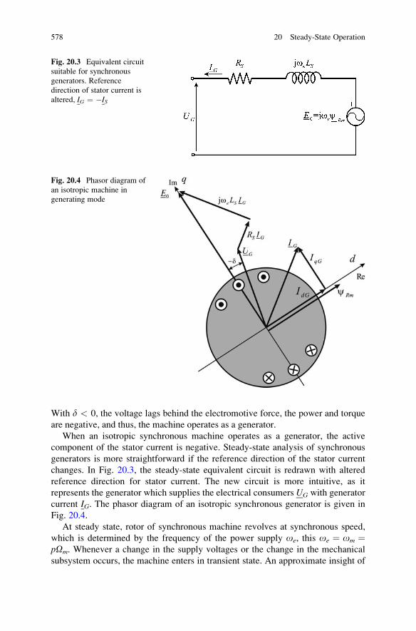
With d < 0, the voltage lags behind the electromotive force, the power and torque
are negative, and thus, the machine operates as a generator.
When an isotropic synchronous machine operates as a generator, the active
component of the stator current is negative. Steady-state analysis of synchronous
generators is more straightforward if the reference direction of the stator current
changes. In Fig. 20.3, the steady-state equivalent circuit is redrawn with altered
reference direction for stator current. The new circuit is more intuitive, as it
represents the generator which supplies the electrical consumers UG with generator
current IG. The phasor diagram of an isotropic synchronous generator is given in
Fig. 20.4.
At steady state, rotor of synchronous machine revolves at synchronous speed,
which is determined by the frequency of the power supply oe, this oe ¼ om ¼pOm. Whenever a change in the supply voltages or the change in the mechanical
subsystem occurs, the machine enters in transient state. An approximate insight of
Fig. 20.3 Equivalent circuit
suitable for synchronous
generators. Reference
direction of stator current is
altered, IG ¼ �IS
Fig. 20.4 Phasor diagram of
an isotropic machine in
generating mode
578 20 Steady-State Operation
transient behavior of the machine can be obtained from the phasor diagram in
Fig. 20.2. In a thought experiment with synchronous motor, a sudden increase in the
load torque Tm results in a decrease of the rotor speed. The stator voltage vectors
revolve at the speed Oe, determined by the supply frequency, while the motion of
the electromotive force is determined by the rotor speed. The speed difference
Oe � Om affects the power angle. The electromotive force E0 revolves at the same
speed as the rotor flux. Therefore, it starts revolving slower than the phasor US,
which revolves at constant, synchronous speed Oe ¼ oe/p. For that reason, the
power angle d starts increasing. According to (20.6), the input power pe increases,which results in an increased electromagnetic torque Tem. An increased Temcounteracts the torque Tm and brings the synchronous machine into a new equilib-
rium, a new steady-state operating conditions.
Question (20.2): Make a phasor diagram for synchronous machine starting from
the example given in Fig. 21.2 and assuming that stator current IS lags behind the
electromotive force by 3p/2. The stator resistance RS is negligible.
Answer (20.2): The electromotive force E0 and the stator voltage US reside on
imaginary axis of the diagram. The voltage amplitude is smaller than the
electromotive force by the amount of XSIS.
Question (20.3): A two-pole synchronous machine operates at steady state with
power angle of d ¼ 0. The stator voltage amplitude is equal to the no load
electromotive force. With US ¼ E0, the stator current is equal to zero. At instant
t ¼ 0, the shaft is loaded by the torque Tm in direction opposite to motion. Discuss
the changes in the rotor speed. Assume that the number of pole pairs is p ¼ 1,
resulting in Om ¼ om and Oe ¼ oe.
Answer (20.3): At steady state, the rotor revolves at synchronous speed.
Therefore, relative position of the stator voltage US and the electromotive force
E0 does not change. With d ¼ 0 and US ¼ E0, there is no stator current and no
electromagnetic torque. The change of the rotor speed is determined by J dOm/
dt ¼ Tem � Tm. Following the increase of the load torque, the rotor speed
decreases. The rotor starts lagging behind the voltage US and it falls behind the
stator magnetic field. The voltage phasor US leads with respect to E0; thus, the
angle d increases. This increase affects the input electrical power Pe and
the electromagnetic torque Tem. As the torque Tem increases with d, it compensates
the increase in the load torque Tm and prevents further decrease of the rotor speed.
For this transient to decay, it is necessary to restore the rotor speedOm < Oe to the
synchronous speed Oe. Therefore, the torque Tem must exceed the motion resis-
tance torque Tm for a brief interval of time, so as to achieve a positive value of
acceleration dOm/dt. This short interval of acceleration is required to restore the
rotor speed to the original value, to the synchronous speed Oe. Derivative dd/dt ofpower angle is determined by the difference between the synchronous speed and
the rotor speed, dd/dt ¼ oe–om ¼ p(Oe � Om). New state of equilibrium is
reached when oe ¼ om, resulting in dd/dt ¼0.
20.4 Phasor Diagram of Isotropic Machine 579
According to (20.6), the power of synchronous machine depends on no load
electromotive force, on stator voltage, and on power angle. Electromotive force E0
is determined by the excitation current. Different pairs of values (E0, d) produce thesame power and the same torque, provided that the product E0sin(d) remains
unchanged. Hence, the machine can maintain the same power with different values
of the excitation current and different values of the excitation fluxCRm. This degree
of freedom can be used for to adjust reactive power Qe (20.6) exchanged between
the machine and the supply network.
Considering the sign of reactive power Qe, there is convention to consider
positive the reactive power taken from the network and delivered to electrical
loads of inductive character, such as coils, where the load current lags behind the
supply voltage. Reactive power taken from the network by receivers such as
capacitors is considered negative. Capacitor current leads with respect to the supply
voltage. All the loads of this nature can be considered as generators of reactive
power. Majority of loads and devices connected to distribution networks are of
inductive nature, including electrical motors, transformers, and all the devices that
include a series inductance. Parallel capacitors are often connected and used as
reactive power compensators that make up for the reactive power generated by
other loads.
On the basis of (20.5), reactive power taken from the network by an isotropic
synchronous machine is equal to
Qe ¼ 3USn USn � E0 cos dð Þð Þ
XS: (20.7)
By reducing the excitation current IR, no load electromotive force E0 ¼ omLmIRreduces as well, and it may become smaller than the voltage of the network. With
USn > E0, reactive power Qe is positive; therefore, the machine acts as an inductive
load. With sufficient increase in excitation current and electromotive force E0,
expression (20.7) becomes negative. Thus, the increase in excitation current results
in negative values of reactive power. In such case, machine acts as a capacitive
load. Hence, the change in excitation current changes the electromotive force and
makes the machine absorb or produce reactive power Qe.
Synchronous generators in hydroelectric and thermal power plants supply
active power consumed by all the electrical loads that are connected to the
power grid. Most of electrical loads have inductive nature, and they absorb
reactive power. Therefore, besides generating the active power, most generators
provide reactive power as well. The amount of reactive power produced by
generators is controlled by the excitation current. In a symmetrical three-phase
system with sinusoidal voltages and currents, relation S2 ¼ P2 þ Q2 connects
apparent power S, active power P, and reactive power Q. Apparent power S in
continuous service is limited by rated voltages and currents. Therefore, an
increase in reactive power reduces the available active power that the machine
can deliver in continuous service.
580 20 Steady-State Operation
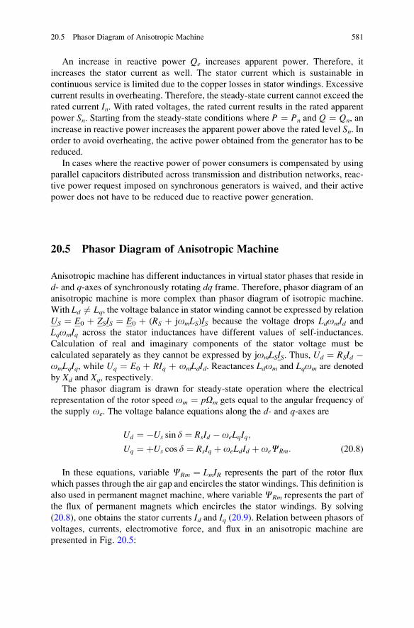
An increase in reactive power Qe increases apparent power. Therefore, it
increases the stator current as well. The stator current which is sustainable in
continuous service is limited due to the copper losses in stator windings. Excessive
current results in overheating. Therefore, the steady-state current cannot exceed the
rated current In. With rated voltages, the rated current results in the rated apparent
power Sn. Starting from the steady-state conditions where P ¼ Pn and Q ¼ Qn, an
increase in reactive power increases the apparent power above the rated level Sn. Inorder to avoid overheating, the active power obtained from the generator has to be
reduced.
In cases where the reactive power of power consumers is compensated by using
parallel capacitors distributed across transmission and distribution networks, reac-
tive power request imposed on synchronous generators is waived, and their active
power does not have to be reduced due to reactive power generation.
20.5 Phasor Diagram of Anisotropic Machine
Anisotropic machine has different inductances in virtual stator phases that reside in
d- and q-axes of synchronously rotating dq frame. Therefore, phasor diagram of an
anisotropic machine is more complex than phasor diagram of isotropic machine.
With Ld 6¼ Lq, the voltage balance in stator winding cannot be expressed by relationUS ¼ E0 þ ZSIS ¼ E0 þ (RS þ jomLS)IS because the voltage drops LdomId and
LqomIq across the stator inductances have different values of self-inductances.
Calculation of real and imaginary components of the stator voltage must be
calculated separately as they cannot be expressed by jomLSIS. Thus, Ud ¼ RSId �omLqIq, while Uq ¼ E0 þ RIq þ omLdId. Reactances Ldom and Lqom are denoted
by Xd and Xq, respectively.
The phasor diagram is drawn for steady-state operation where the electrical
representation of the rotor speed om ¼ pOm gets equal to the angular frequency of
the supply oe. The voltage balance equations along the d- and q-axes are
Ud ¼ �Us sin d ¼ RsId � oeLqIq;
Uq ¼ þUs cos d ¼ RsIq þ oeLdId þ oeCRm: (20.8)
In these equations, variable CRm ¼ LmIR represents the part of the rotor flux
which passes through the air gap and encircles the stator windings. This definition is
also used in permanent magnet machine, where variable CRm represents the part of
the flux of permanent magnets which encircles the stator windings. By solving
(20.8), one obtains the stator currents Id and Iq (20.9). Relation between phasors of
voltages, currents, electromotive force, and flux in an anisotropic machine are
presented in Fig. 20.5:
20.5 Phasor Diagram of Anisotropic Machine 581
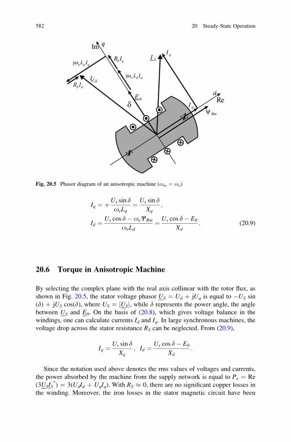
Iq ¼ þUs sin doeLq
¼ Us sin dXq
;
Id ¼ Us cos d� oeCRm
oeLd¼ Us cos d� E0
Xd: (20.9)
20.6 Torque in Anisotropic Machine
By selecting the complex plane with the real axis collinear with the rotor flux, as
shown in Fig. 20.5, the stator voltage phasor US ¼ Ud þ jUq is equal to �US sin
(d) þ jUS cos(d), where US ¼ jUSj, while d represents the power angle, the angle
between US and E0. On the basis of (20.8), which gives voltage balance in the
windings, one can calculate currents Id and Iq. In large synchronous machines, the
voltage drop across the stator resistance RS can be neglected. From (20.9),
Iq ¼ Us sin dXq
; Id ¼ Us cos d� E0
Xd:
Since the notation used above denotes the rms values of voltages and currents,
the power absorbed by the machine from the supply network is equal to Pe ¼ Re
(3USIS*) ¼ 3(UdId þ UqIq). With RS � 0, there are no significant copper losses in
the winding. Moreover, the iron losses in the stator magnetic circuit have been
Fig. 20.5 Phasor diagram of an anisotropic machine (om ¼ oe)
582 20 Steady-State Operation
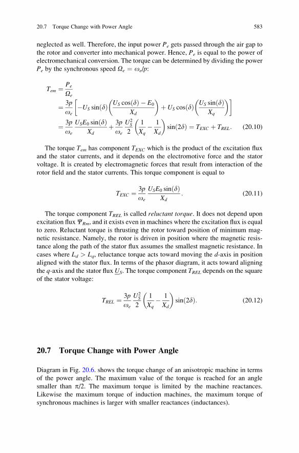
neglected as well. Therefore, the input power Pe gets passed through the air gap to
the rotor and converter into mechanical power. Hence, Pe is equal to the power of
electromechanical conversion. The torque can be determined by dividing the power
Pe by the synchronous speed Oe ¼ oe/p:
Tem ¼ Pe
Oe
¼ 3p
oe�US sin dð Þ US cos dð Þ � E0
Xd
� �þ US cos dð Þ US sin dð Þ
Xq
� �� �
¼ 3p
oe
USE0 sin dð ÞXd
þ 3p
oe
U2S
2
1
Xq� 1
Xd
� �sin 2dð Þ ¼ TEXC þ TREL: (20.10)
The torque Tem has component TEXC which is the product of the excitation flux
and the stator currents, and it depends on the electromotive force and the stator
voltage. It is created by electromagnetic forces that result from interaction of the
rotor field and the stator currents. This torque component is equal to
TEXC ¼ 3p
oe
USE0 sin dð ÞXd
: (20.11)
The torque component TREL is called reluctant torque. It does not depend upon
excitation fluxCRm, and it exists even in machines where the excitation flux is equal
to zero. Reluctant torque is thrusting the rotor toward position of minimum mag-
netic resistance. Namely, the rotor is driven in position where the magnetic resis-
tance along the path of the stator flux assumes the smallest magnetic resistance. In
cases where Ld > Lq, reluctance torque acts toward moving the d-axis in position
aligned with the stator flux. In terms of the phasor diagram, it acts toward aligning
the q-axis and the stator flux US. The torque component TREL depends on the squareof the stator voltage:
TREL ¼ 3p
oe
U2S
2
1
Xq� 1
Xd
� �sin 2dð Þ: (20.12)
20.7 Torque Change with Power Angle
Diagram in Fig. 20.6. shows the torque change of an anisotropic machine in terms
of the power angle. The maximum value of the torque is reached for an angle
smaller than p/2. The maximum torque is limited by the machine reactances.
Likewise the maximum torque of induction machines, the maximum torque of
synchronous machines is larger with smaller reactances (inductances).
20.7 Torque Change with Power Angle 583
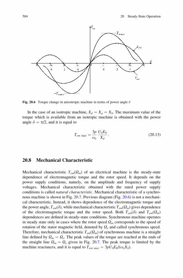
In the case of an isotropic machine, Xd ¼ Xq ¼ XS. The maximum value of the
torque which is available from an isotropic machine is obtained with the power
angle d ¼ p/2, and it is equal to
Tem max ¼ 3p
oe
USE0
Xd: (20.13)
20.8 Mechanical Characteristic
Mechanical characteristic Tem(Om) of an electrical machine is the steady-state
dependence of electromagnetic torque and the rotor speed. It depends on the
power supply conditions, namely, on the amplitude and frequency of supply
voltages. Mechanical characteristic obtained with the rated power supply
conditions is called natural characteristic. Mechanical characteristic of a synchro-
nous machine is shown in Fig. 20.7. Previous diagram (Fig. 20.6) is not a mechani-
cal characteristic. Instead, it shows dependence of the electromagnetic torque and
the power angle, Tem(d), while mechanical characteristic Tem(Om) gives dependence
of the electromagnetic torque and the rotor speed. Both Tem(d) and Tem(Om)
dependences are defined in steady-state conditions. Synchronous machine operates
in steady state only in cases where the rotor speed Om corresponds to the speed of
rotation of the stator magnetic field, denoted by Oe and called synchronous speed.
Therefore, mechanical characteristic Tem(Om) of synchronous machine is a straight
line defined by Om ¼ Oe. The peak values of the torque are reached at the ends of
the straight line Om ¼ Oe given in Fig. 20.7. The peak torque is limited by the
machine reactances, and it is equal to Tem max ¼ 3pUSE0/(oeXS).
Fig. 20.6 Torque change in anisotropic machine in terms of power angle d
584 20 Steady-State Operation
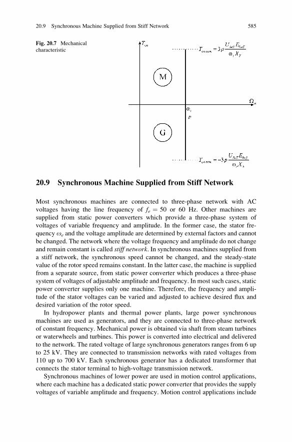
20.9 Synchronous Machine Supplied from Stiff Network
Most synchronous machines are connected to three-phase network with AC
voltages having the line frequency of fe ¼ 50 or 60 Hz. Other machines are
supplied from static power converters which provide a three-phase system of
voltages of variable frequency and amplitude. In the former case, the stator fre-
quency oe and the voltage amplitude are determined by external factors and cannot
be changed. The network where the voltage frequency and amplitude do not change
and remain constant is called stiff network. In synchronous machines supplied from
a stiff network, the synchronous speed cannot be changed, and the steady-state
value of the rotor speed remains constant. In the latter case, the machine is supplied
from a separate source, from static power converter which produces a three-phase
system of voltages of adjustable amplitude and frequency. In most such cases, static
power converter supplies only one machine. Therefore, the frequency and ampli-
tude of the stator voltages can be varied and adjusted to achieve desired flux and
desired variation of the rotor speed.
In hydropower plants and thermal power plants, large power synchronous
machines are used as generators, and they are connected to three-phase network
of constant frequency. Mechanical power is obtained via shaft from steam turbines
or waterwheels and turbines. This power is converted into electrical and delivered
to the network. The rated voltage of large synchronous generators ranges from 6 up
to 25 kV. They are connected to transmission networks with rated voltages from
110 up to 700 kV. Each synchronous generator has a dedicated transformer that
connects the stator terminal to high-voltage transmission network.
Synchronous machines of lower power are used in motion control applications,
where each machine has a dedicated static power converter that provides the supply
voltages of variable amplitude and frequency. Motion control applications include
Fig. 20.7 Mechanical
characteristic
20.9 Synchronous Machine Supplied from Stiff Network 585
propulsion of vehicles, control of industrial robots, motion tasks in production
machines, and other similar tasks where it is necessary to provide a continuous
change of the rotor position, speed, and torque. In motion control applications,
synchronous machines operate mostly as motors which overcome the motion
resistances within work machines. In speed control loops, synchronous motors
are used as torque actuators, and their task is to provide the torque which
corresponds to the torque command. The torque command is calculated within
the speed controller, and it corresponds to the torque required to overcome the
motion resistances and to achieve desired variation of the speed. Providing variable
torque at variable rotor speed requires the stator voltage frequency and amplitude to
be changed in continuous manner. This is achieved by supplying the stator winding
from three-phase inverters which comprise semiconductor power switches and
operate on pulse width modulation principles.
It is of interest to study operation of synchronous machines in both cases that are
mentioned above. The first to consider is the operation of synchronous machines
supplied from a stiff network. The subsequent analysis considers three-phase
synchronous machine connected to three-phase network with symmetrical AC
voltages, wherein the voltages have constant line frequency and constant amplitude.
Without the lack of generality, it is assumed that the shaft of synchronous machine
is connected to driving turbine which provides the source of mechanical work and
that the synchronous machine operates as a generator which converts mechanical
work into electrical energy. The steady-state performance of synchronous machine
is considered, described by the steady-state equivalent circuit in Fig. 20.1, phasor
diagram in Fig. 20.2. In further discussion, it is of interest to investigate the impact
of changes in the power angle d on the electromagnetic torque (20.3), active and
reactive power (20.5). In steady-state conditions, gradual changes in the torque of
the driving turbine result in changes of the power angle and the active power, while
the changes in excitation current affect the reactive power.
20.10 Operation of Synchronous Generators
Synchronous generators in thermal and hydropower plants have the rated voltages
that range from 6 to 25 kV and rated power that ranges from several tens of MW up
to several hundreds of MW. Generator shaft is coupled to a steam turbine or a water
turbine which provides the driving torque TT > 0. This torque supports the motion
of the rotor; thus, Newton equation of motion has the form JdOm/dt ¼ Tem þ TT. Atsteady state, dOm/dt ¼ 0; thus, the electromagnetic torque of the generator is
negative and equal to Tem ¼ �TT. The power of electromechanical conversion
Pe ¼ TmOm is also negative, illustrating the fact that the electromechanical energy
conversion within the machine has opposite direction, since the mechanical work
gets converter into electrical energy. In the phase diagram of generator (Fig. 20.4),
the electromotive force E0 leads with respect to the voltage US; thus, the power
586 20 Steady-State Operation
angle d is negative. Power Pe delivered to the machine from the network is negative
in generator mode, and it is equal to
Pe ¼ 3USnE0
XSsin dð Þ ¼ �PG; (20.14)
where PG denotes the active power delivered from the generator to the network.
Assuming that the network has a constant line frequency, the change in power angle
is described by dd/dt ¼ oe � pOm. With constant oe, an increase in the rotor
speed causes the power angle to reduce. An equilibrium point is reached when
Om ¼ oe/p.It is of interest to study behavior of synchronous generators in cases where the
driving turbine torque TT exhibits small changes and also in cases where the line
frequencies oe changes by a very small amount.
20.10.1 Increase of Turbine Power
The power of steam turbines or water turbines can be increased or decreased
according to requirements. Variation of the steam turbine power is achieved by
means of opening or closing the valves that feed the steam from the boiler to the
steam turbine and also by operating the valves that change the air and coal dust
supply to the boiler. The power of a water turbine changes in a similar manner. An
increased turbine power results in a larger turbine torque TT which is passed to the
synchronous generator, where it tends to increase the rotor speed. Starting from the
state of equilibrium where Tem0 ¼ �TT0, an increase of the turbine torque to a newvalue of TT1 ¼ TT0 þ DT leads to an increase of the rotor speed according to
equation JdOm /dt ¼ Tem þ TT ¼ þDT.An increase of the rotor speed changes the power angle d according to dd/
dt ¼ oe � pOm. The motion of the electromotive force E0 ¼ jpOmCRm is deter-
mined by the rotor speed, while the voltage US rotates at synchronous speed
Oe ¼ oe/p, determined by the network frequency. With an increase in the rotor
speed, the power angle delta decreases, and the phase lead �d of electromotive
force with respect to the stator voltage increases. The power angle assumes negative
values in generator mode, and it goes further in negative direction. The generator
power PG ¼ �Pe ¼ �3(USnE0/XS)sin(d) is increased. Along with that, the electro-magnetic torque Tem ¼ Pe/Oe < 0 increases in magnitude. With JdOm/dt ¼ Tem þTT, a new equilibrium with JdOm/dt ¼ 0 can be reached when the electromagnetic
torque reaches the value of Tem ¼ �TT1. The nature of transient phenomena that
take place while reaching the new equilibrium is discussed later. In this new steady
state, electrical power delivered by the generator to the transmission network is
increased. It is assumed that the excess power in the network gets counteracted by
an increase in electrical power consumption of electrical loads that are connected to
the network. If the assumption that the network is stiff holds, the end of the excess
20.10 Operation of Synchronous Generators 587
power does not put in question the above considerations. In an actual network,
however large, the line frequency may exhibit small changes in consequence to
variation in electrical power consumption or variation in mechanical power deliv-
ered by steam and water turbines.
In a thought experiment with an electrical network that has several generators
and a number of constant power electrical consumers, it is of interest to consider the
events that take place when all the steam and water turbines increase their mechan-
ical power at the same time. If all the electrical consumers retain the same power,
then the sum of power generated by all the generators in the network must remain
constant as well. Namely, unless otherwise stated, the network does not have means
to accumulate or store the excess of electrical energy. Therefore, the sum of power
generated by all the synchronous generators has to remain constant. With PG ¼�Pe ¼ const., the electromagnetic torque Tem has to remain constant as well.
According to Newton equation of motion JdOm/dt ¼ Tem þ TT, an increase in TTin conditions where Tem remains constant results in an increase of the rotor speed.
Hence, in the considered thought experiment, the rotor speed in all generators will
increase, increasing in such way the line frequency of the considered network.
Excess energy that comes from the steam and water turbines is not converted into
electrical energy. Instead, it is stored as kinetic energy of revolving masses, Wkin
¼ P12JOm
2. If the situation with excess turbine power persists, the line frequency
of the network is continuously increased due to continuous increase in the rotor
speed of synchronous machines.
In practical power networks, an increase in the line frequency indicates the
excess power received from the steam and water turbines, while a decrease in the
line frequency indicates the lack of mechanical power delivered to generators and/
or an excessive consumption.
Question (20.4): The problem statement relies on the above thought experiment,
where the power of steam and water turbines increases, where the power of
electrical consumers remains constant, and where the rotor speed and the line
frequency increase. Assume that the power system considered above has one
high-voltage transmission line connected to a much larger power system. This
second, larger power system can be treated as a stiff network. Series reactance XS
of the transmission line is known, as well as the voltage amplitudesU1 andU2 of the
two power systems. Both systems have symmetrical systems of three-phase
voltages. Consider the effects of such connection on the behavior of the system
with the excess power.
Answer (20.4): The two electrical power systems with voltages U1 and U2,
connected by means of the transmission line with the series reactance X, can be
represented as two voltage sources connected by a series impedance jX. Thisrepresentation is similar to the equivalent circuit in Fig. 20.1, where the voltage
US gets connected to the voltage E0 across the series impedance.
588 20 Steady-State Operation
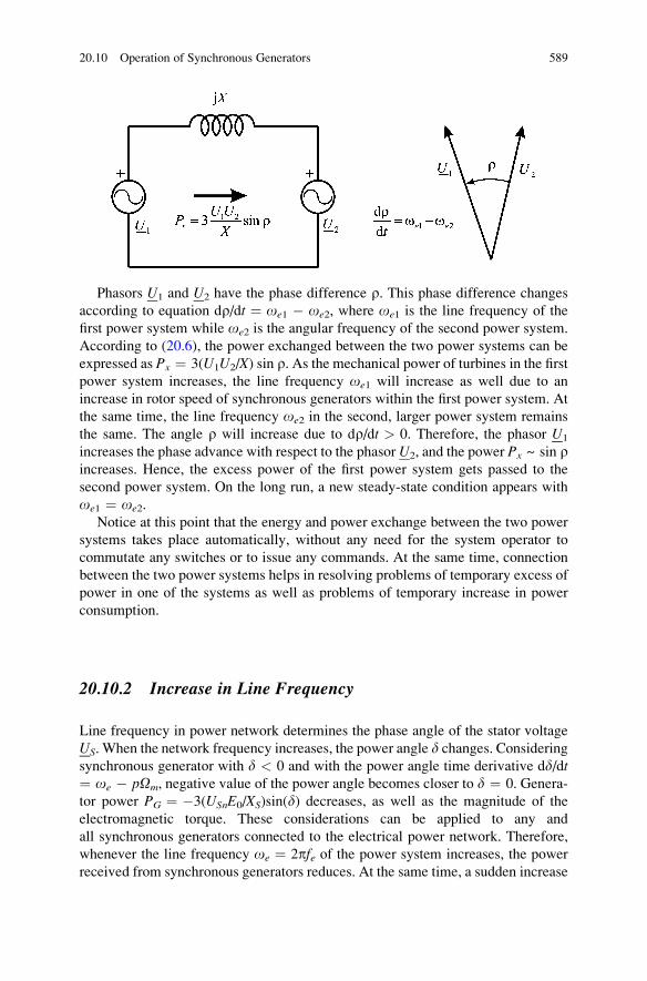
Phasors U1 and U2 have the phase difference r. This phase difference changes
according to equation dr/dt ¼ oe1 � oe2, where oe1 is the line frequency of the
first power system while oe2 is the angular frequency of the second power system.
According to (20.6), the power exchanged between the two power systems can be
expressed as Px ¼ 3(U1U2/X) sin r. As the mechanical power of turbines in the first
power system increases, the line frequency oe1 will increase as well due to an
increase in rotor speed of synchronous generators within the first power system. At
the same time, the line frequency oe2 in the second, larger power system remains
the same. The angle r will increase due to dr/dt > 0. Therefore, the phasor U1
increases the phase advance with respect to the phasor U2, and the power Px ~ sin rincreases. Hence, the excess power of the first power system gets passed to the
second power system. On the long run, a new steady-state condition appears with
oe1 ¼ oe2.
Notice at this point that the energy and power exchange between the two power
systems takes place automatically, without any need for the system operator to
commutate any switches or to issue any commands. At the same time, connection
between the two power systems helps in resolving problems of temporary excess of
power in one of the systems as well as problems of temporary increase in power
consumption.
20.10.2 Increase in Line Frequency
Line frequency in power network determines the phase angle of the stator voltage
US. When the network frequency increases, the power angle d changes. Consideringsynchronous generator with d < 0 and with the power angle time derivative dd/dt¼ oe � pOm, negative value of the power angle becomes closer to d ¼ 0. Genera-
tor power PG ¼ �3(USnE0/XS)sin(d) decreases, as well as the magnitude of the
electromagnetic torque. These considerations can be applied to any and
all synchronous generators connected to the electrical power network. Therefore,
whenever the line frequency oe ¼ 2pfe of the power system increases, the power
received from synchronous generators reduces. At the same time, a sudden increase
20.10 Operation of Synchronous Generators 589
of power consumed by electrical loads reduces the speed of revolving rotors and
causes a decrease in the line frequency.
On the basis of the above examples, it can be concluded that electrical power
systems with synchronous generators have a strong coupling between the power
and the line frequency. This P-f relation is one of basic power system properties,
and it provides the grounds for the power regulation and the frequency regulation.
20.10.3 Reactive Power and Voltage Changes
A synchronous generator delivers the power PG ¼ �3(USnE0/XS)sin(d) with differ-ent values of the electromotive force and different values of power angle. In order to
maintain a constant power, it is of interest to keep the product E0sin(d) constant.The electromotive force E0 can be varied by changing the excitation current of the
generator. It is possible to change the excitation current, to change the fluxCRm and
the electromotive force E0 ¼ omCRm, and yet to maintain the same power,
provided that the product E0sin(d) remains the same. This degree of freedom can
be used to change the reactive power Qe absorbed by the machine from the three-
phase network. Reactive power of an isotropic synchronous machine is proportional
to the voltage difference between the stator voltage and the electromotive force E0:
Qe ¼ 3USn USn � E0 cos dð Þð Þ
XS: (20.15)
By increasing the excitation current IR, electromotive force E0 ¼ omLmIRbecomes larger than the stator voltage; thus, the reactive power Qe becomes
negative. In this way, synchronous generator becomes a source of reactive power,
and its equivalent impedance has capacitive nature. Majority of electrical
consumers has an inductive power factor and consumes reactive power, behaving
as a coil. Therefore, electrical power system must comprise adequate sources of
reactive power.
Transmission of reactive power across transmission and distribution line results
in significant voltage drops. Most transmission lines have their equivalent series
reactance X considerably larger than equivalent series resistance R. In cases where athree-phase electrical load gets connected at the end of the transmission line, where
it absorbs reactive power Q and has the voltage UEND ¼ UEND, the current of
the transmission line is equal to I ¼ �jQ/(3UEND). The voltage at the beginning
of the transmission line is equal to UBEG ¼ UEND þ jXI ¼ UEND þ XQ/(3UEND).
The voltage drop jXI is collinear (in phase) with the voltages. Hence, the value XI isdirectly subtracted from UBEG in order to obtain UEND.
Notice at this point that replacing reactive power consumer by resistive load
which absorbs active power P ¼ Q results in a significant reduction of the voltage
drop. With resistive load, the current of the same amplitude results in much smaller
590 20 Steady-State Operation
difference in amplitudes of UBEG and UEND. With I ¼ P/(3UEND), UBEG ¼ UEND
þ jXP/(3UEND). The voltage drop jXI is perpendicular (phase shifted by p/2) withrespect to UEND, and this circumstance results in jUBEGj � jUENDj << XI.
Whenever electrical loads absorb reactive power, there are considerable voltage
drops across the transmission lines. As a consequence, it is necessary to increase the
stator voltage of synchronous generators in order to maintain constant voltage at
electrical loads. For this to achieve, it is necessary to increase the excitation
current IR of synchronous generators, which leads to increased flux CRm and
increased electromotive force E0. At the same time, an increase in E0 contributes
to increased reactive power delivered from generators to the network.
From the above considerations, it is concluded that the voltage across the
network and the reactive power flow are strongly related. This U-Q relation
constitutes the bases for the voltage control in electric power systems.
20.10.4 Changes in Power Angle
Changes in mechanical power received from steam or water turbines result in
transient response of synchronous machine which ends in a new steady-state
condition with a different value of power angle. A sudden increase in electrical
load of the generator produces the same effect. It is of interest to investigate the
transient response of the machine torque, power, and power angle during such
transients.
With constant power supply frequency, the stator voltage vector rotates at
constant synchronous speed Oe ¼ oe/p, determined by the supply frequency oe.
The rotor flux is created by the current IR in the excitation winding, which revolves
with the rotor. Therefore, the vector of the rotor flux revolves at the rotor speed Om.
The excitation fluxCRm creates the electromotive force E0 ¼ jCRmOm in the stator
windings. In steady state, the stator voltage and electromotive force are represented
by phasors US and E0. Power angle d represents the difference in initial phases
of the stator voltage and the electromotive force. It changes according to the law3
dd/dt ¼ oe � om ¼ oe � pOm. The phase of the stator voltage depends on
the supply frequency oe, while the phase of the electromotive force depends on
the rotor speed pOm. Therefore, changes in power angle d are defined by the speed
difference between the synchronous speed and the rotor speed. At the same time,
the electromagnetic torque of synchronous machine operating in the steady state
depends on the product of US, E0, and sine of the power angle.
3 In phasor diagrams, phasors US and E0 represent an AC stator voltage and an AC electromotive
force. The power angle d represents the phase difference or the electrical shift between the stator
voltage and the electromotive force. Therefore, the first-time derivative of power angle is equal to
dd/dt ¼ p(Oe � Om) ¼ oe � pOm ¼ oe � om, where p is the number of pole pairs.
20.10 Operation of Synchronous Generators 591
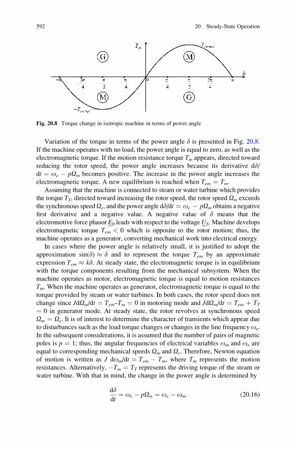
Variation of the torque in terms of the power angle d is presented in Fig. 20.8.
If the machine operates with no load, the power angle is equal to zero, as well as the
electromagnetic torque. If the motion resistance torque Tm appears, directed toward
reducing the rotor speed, the power angle increases because its derivative dd/dt ¼ oe � pOm becomes positive. The increase in the power angle increases the
electromagnetic torque. A new equilibrium is reached when Tem ¼ Tm.Assuming that the machine is connected to steam or water turbine which provides
the torque TT, directed toward increasing the rotor speed, the rotor speed Om exceeds
the synchronous speedOe, and the power angle dd/dt ¼ oe � pOm obtains a negative
first derivative and a negative value. A negative value of d means that the
electromotive force phasor E0 leads with respect to the voltageUS. Machine develops
electromagnetic torque Tem < 0 which is opposite to the rotor motion; thus, the
machine operates as a generator, converting mechanical work into electrical energy.
In cases where the power angle is relatively small, it is justified to adopt the
approximation sin(d) � d and to represent the torque Tem by an approximate
expression Tem � kd. At steady state, the electromagnetic torque is in equilibrium
with the torque components resulting from the mechanical subsystem. When the
machine operates as motor, electromagnetic torque is equal to motion resistances
Tm. When the machine operates as generator, electromagnetic torque is equal to the
torque provided by steam or water turbines. In both cases, the rotor speed does not
change since JdOm/dt ¼ Tem–Tm ¼ 0 in motoring mode and JdOm/dt ¼ Tem þ TT¼ 0 in generator mode. At steady state, the rotor revolves at synchronous speed
Om ¼ Oe. It is of interest to determine the character of transients which appear due
to disturbances such as the load torque changes or changes in the line frequency oe.
In the subsequent considerations, it is assumed that the number of pairs of magnetic
poles is p ¼ 1; thus, the angular frequencies of electrical variables om and oe are
equal to corresponding mechanical speeds Om and Oe. Therefore, Newton equation
of motion is written as J dom/dt ¼ Tem � Tm, where Tm represents the motion
resistances. Alternatively, �Tm ¼ TT represents the driving torque of the steam or
water turbine. With that in mind, the change in the power angle is determined by
dddt
¼ oe � pOm ¼ oe � om: (20.16)
Fig. 20.8 Torque change in isotropic machine in terms of power angle
592 20 Steady-State Operation
Newton equation for a two-pole machine takes the form
JdOm
dt¼ J
dom
dt¼ Tem � Tm; (20.17)
while the change in the power angle depends on differential equation
Jd2ddt2
¼ �Tem dð Þ þ Tm: (20.18)
Staring from no load conditions where d ¼ 0, Tem ¼ 0, and om ¼ oe, and
introducing the step change in the load torque Tm (or the turbine torque TT), atransient interval follows where the rotor speed, electromagnetic torque, and power
angle change and fluctuate before entering another steady-state condition. During
these transients, the rotor speed is not equal to the synchronous speed. Taking into
account that position of the dq coordinate system is determined by the rotor
position, while the vector of the stator voltage depends on the power supply
frequency, it is concluded that the stator voltage vector will move with respect to
selected dq coordinate frame. For this reason, projections Ud and Uq of the stator
voltage vector US on the axes of dq frame will change during transients. Electrical
subsystem of synchronous machine is represented by voltage balance equations
in virtual stator phases that are placed in d-axis and q-axis of dq frame. Changes in
corresponding voltages Ud and Uq introduce nonzero derivatives of flux linkages
Cd and Cq, thus bringing the electrical subsystem in transient state. Hence, during
transients in mechanical subsystem, where the electromagnetic torque, the rotor
speed, and the power angle exhibit transient changes, the electrical subsystem of
synchronous machine does not remain in steady-state condition, and it enters
transient state of its own.
While in transient state, electrical subsystem of synchronous machines cannot be
represented by the steady-state equivalent circuit. At the same time, the transient
torque cannot be represented by simplified expression such as Tem � kd, which is
derived from the steady-state equivalent circuit.
Within the next chapter, it will be shown that the time constants of mechanical
subsystems are considerably larger than the time constants of electrical subsystem.
This circumstance will be used to simplify transient analysis of synchronous
machines.
20.10 Operation of Synchronous Generators 593
Chapter 21
Transients in Sychronous Machines
In this chapter, transient response of synchronous machines connected to stiff
network is analyzed and discussed. Analysis of transients in electrical and mechan-
ical subsystems of synchronous machines is relatively complex due to a relatively
large number of state variables, such as the rotor position and speed, and the
winding currents and flux linkages. Complexity of mathematical model does not
help the process of understanding the nature of transients and hinders deriving
corresponding conclusions. The analysis can be simplified by introducing the
assumption that transients in electrical subsystem decay considerably faster than
those of mechanical subsystem. In this way, analysis of transients in mechanical
subsystem can be performed by using steady state model of electrical subsystem.
In this way, results are made more legible and intuitive.
This chapter begins with introducing and explaining the time constants that
characterize transient response in electrical subsystem and mechanical subsystem
of synchronous machines. For synchronous machine supplied from stiff network,
electromagnetic torque is expressed in terms of the power angle. Transient response
of the rotor speed, power angle, and the electromagnetic torque is obtained from
Newton differential equation of motion, and from the torque-power angle relation.
Damper winding is introduced and explained as the means of suppressing
oscillations of the torque, power, and speed caused by sudden changes at electrical
or mechanical accesses to the machine. Some typical realizations of damper
winding are introduced and discussed.
In the second half of this chapter, analysis is focused on the short-circuit
transient in synchronous generators. Short-circuit analysis is simplified by the
assumption that transient processes in damper windings are the first to decay during
the subtransient interval. Within the subsequent interval called transient interval,
transient processes in excitation winding cease. Eventually, transient phenomena
disappear, and the stator current reduces to steady state short-circuit current.
A series of reasonable assumptions and engineering considerations results in
deriving subtransient and transient time constants, and in subtransient, transient,
and steady state reactances and short-circuit currents. This chapter ends by
indicating most typical values of relevant time constants and reactances.
S.N. Vukosavic, Electrical Machines, Power Electronics and Power Systems,
DOI 10.1007/978-1-4614-0400-2_21, # Springer Science+Business Media New York 2013
595
21.1 Electrical and Mechanical Time Constants
Transient phenomena in electrical subsystem have to do with winding currents and
flux linkages in the air gap and in corresponding magnetic circuits. Transient
response in machine windings is characterized by electrical time constants. Electri-
cal current in a winding of resistance R, with self-inductance L and with the voltage
u ¼ 0, decays exponentially, according to the law i(t) ¼ i(0)∙e�t/t, where t ¼ L/Ris the electrical time constant of the winding. The change i(t) ¼ i(0)∙e�t/t, the
winding current takes place in cases where the winding does not have any coupling
with other windings. In synchronous machines, the stator phase windings and the
excitation winding are coupled, and they interact and affect the change of currents
and flux linkages. Therefore, transient response may not be exponential, and
the time constant can be different than t ¼ L/R. Nonetheless, the time constant
t ¼ L/R serves as a rough description of dynamic processes in electrical subsystem.
In smaller machines, time constants of the windings are of the order of several tens
of milliseconds, while high-power machines have time constants t ¼ L/R in excess
to 1 s. On the other hand, transient phenomena in mechanical subsystem are
considerably slower. Synchronous generators have massive rotors with significant
inertia. They are coupled to steam or water turbines with certain inertia J as well.Due to large inertia, rotor speed changes, and transient phenomena in mechanical
subsystem are considerably longer than the time constants of electrical subsystem.
With that in mind, analysis of transients in mechanical subsystem can be simplified.
While introducing disturbances into mechanical subsystem, such as the torque
changes, electrical subsystem of the machine gets disturbed as well. Due to much
shorter electrical time constants, transient processes in electrical subsystem would
quickly decay. Following that, electrical subsystem can be modeled by steady state
equivalent circuit. For the largest part of the transient process in mechanical
subsystem, electromagnetic torque can be modeled by (20.11) and considered
proportional to sin(d).Neglecting transient phenomena in the windings and considering them much
quicker than transient processes in mechanical subsystem, the changes in electro-
magnetic torque can be considered proportional to sin(d). Analysis of relatively
small torque changes in close vicinity of no load operating point where Tem ¼ 0 and
d ¼ 0, electromagnetic torque can be approximated by Tem � kd.
21.2 Hunting of Synchronous Machines
During transient phenomena, the power angle changes according to dd/dt ¼ oe � om.
The second derivative of the power angle can be determined as d2d/dt2 ¼ doe/dt �dom/dt. Assuming that the supply frequency oe does not change, it follows that dom/
dt ¼ �d2d/dt2. For a two-pole machine where p ¼ 1 andOm ¼ om, Newton equation
of motion takes the form
596 21 Transients in Sychronous Machines
Jd2ddt2
¼ �kdþ Tm: (21.1)
Differential equation (21.1) can be transferred into algebraic equation by applying
Laplace transform. Instead of the time function d(t), algebraic equation has the
complex image L(d(t)) ¼ d(s), where s denotes Laplace operator. It is assumed that
the load torque disturbance Tm(t) changes at instant t ¼ 0 from Tm(0�) ¼ 0 to Tm(0
+)
¼ TM. Prior to the load torque step, the system was in steady state with Tem ¼ 0,
d(0) ¼ 0, and dd/dt(0) ¼ 0. With that in mind, Laplace transform is applied to
differential equation (21.1), and the latter is converted into the following algebraic
equation:
Jd2dðtÞdt2
þ kdðtÞ ¼ TmðtÞ ) Js2dðsÞ þ kdðsÞ ¼ TmðsÞ ¼ TMs:
Complex image Tm(s) ¼ TM/s represents Heaviside function h(t)∙TM which
describes the step increase of the torque at the initial t ¼ 0. Based upon the
above algebraic equation, the power angle d(s) can be expressed in terms of
the torque:
dðsÞ ¼ 1
Js2 þ k
TMs
¼ WðsÞ TMs:
The function W(s) is called transfer function because it relates the input and the
output of the system. Complex image Tm(s) of the load torque Tm(t) is considered tobe the input to the system since the torque changes originate transient phenomena in
the system. Complex image d(s) of the power angle d(t) is the system response, and
it is considered to be the output of the system. Polynomial f(s) ¼ Js2 þ k in
denominator of the transfer function is called characteristic polynomial.Zeros of characteristic polynomial are the roots of equation f(s) ¼ 0, and they are
called poles of the transfer function. These poles determine character of the system
response, namely, whether response is aperiodic or with oscillations. The poles also
determine the response speed and decay time of eventual oscillations. With charac-
teristic polynomial of the form f(s) ¼ (s � s1)(s � s2), which has two finite zeros s1and s2, the system response d(t) to the input step change Tm(t) comprises factors exp
(s1t) and exp(s2t). With s1 ¼ �1/t, the system response comprises factors such
as exp(�t/t). With s1 ¼ �jo0, the system response comprises factors such as exp
(�jo0t) ¼ cos(o0t) � jsin(o0t). With s1 ¼ �1/t � jo0, the system response
comprises factors such as exp(�t/t � jo0t) ¼ exp(�t/t)∙cos(o0t) � j∙exp(�t/t)∙sin(o0t).
Characteristic polynomial f(s) ¼ Js2 þ k has two finite zeros s1/2 ¼ �j∙sqrt(k/J)¼ �jo0. Therefore, the load step response of considered synchronous machine is
oscillatory. According to (21.1), characteristic polynomial has two poles on imagi-
nary axis of s-plane, �jo0. This means that the response does not decay.
21.2 Hunting of Synchronous Machines 597
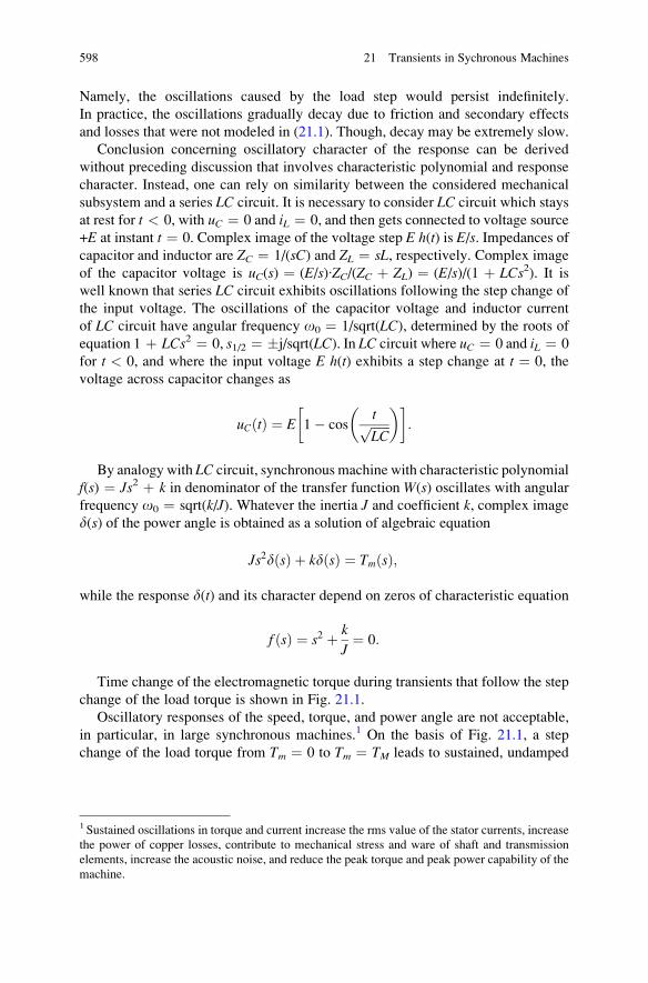
Namely, the oscillations caused by the load step would persist indefinitely.
In practice, the oscillations gradually decay due to friction and secondary effects
and losses that were not modeled in (21.1). Though, decay may be extremely slow.
Conclusion concerning oscillatory character of the response can be derived
without preceding discussion that involves characteristic polynomial and response
character. Instead, one can rely on similarity between the considered mechanical
subsystem and a series LC circuit. It is necessary to consider LC circuit which stays
at rest for t < 0, with uC ¼ 0 and iL ¼ 0, and then gets connected to voltage source
+E at instant t ¼ 0. Complex image of the voltage step E h(t) is E/s. Impedances of
capacitor and inductor are ZC ¼ 1/(sC) and ZL ¼ sL, respectively. Complex image
of the capacitor voltage is uC(s) ¼ (E/s)∙ZC/(ZC þ ZL) ¼ (E/s)/(1 þ LCs2). It iswell known that series LC circuit exhibits oscillations following the step change of
the input voltage. The oscillations of the capacitor voltage and inductor current
of LC circuit have angular frequency o0 ¼ 1/sqrt(LC), determined by the roots of
equation 1 þ LCs2 ¼ 0, s1/2 ¼ �j/sqrt(LC). In LC circuit where uC ¼ 0 and iL ¼ 0
for t < 0, and where the input voltage E h(t) exhibits a step change at t ¼ 0, the
voltage across capacitor changes as
uCðtÞ ¼ E 1� costffiffiffiffiffiffiLC
p� �� �
:
By analogy with LC circuit, synchronous machine with characteristic polynomial
f(s) ¼ Js2 þ k in denominator of the transfer function W(s) oscillates with angular
frequency o0 ¼ sqrt(k/J). Whatever the inertia J and coefficient k, complex image
d(s) of the power angle is obtained as a solution of algebraic equation
Js2dðsÞ þ kdðsÞ ¼ TmðsÞ;
while the response d(t) and its character depend on zeros of characteristic equation
f ðsÞ ¼ s2 þ k
J¼ 0:
Time change of the electromagnetic torque during transients that follow the step
change of the load torque is shown in Fig. 21.1.
Oscillatory responses of the speed, torque, and power angle are not acceptable,
in particular, in large synchronous machines.1 On the basis of Fig. 21.1, a step
change of the load torque from Tm ¼ 0 to Tm ¼ TM leads to sustained, undamped
1 Sustained oscillations in torque and current increase the rms value of the stator currents, increase
the power of copper losses, contribute to mechanical stress and ware of shaft and transmission
elements, increase the acoustic noise, and reduce the peak torque and peak power capability of the
machine.
598 21 Transients in Sychronous Machines
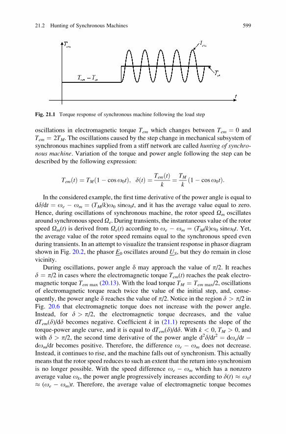
oscillations in electromagnetic torque Tem which changes between Tem ¼ 0 and
Tem ¼ 2TM. The oscillations caused by the step change in mechanical subsystem of
synchronous machines supplied from a stiff network are called hunting of synchro-nous machine. Variation of the torque and power angle following the step can be
described by the following expression:
TemðtÞ ¼ TM 1� coso0tð Þ; dðtÞ ¼ TemðtÞk
¼ TMk
1� coso0tð Þ:
In the considered example, the first time derivative of the power angle is equal to
dd/dt ¼ oe � om ¼ (TM/k)o0 sino0t, and it has the average value equal to zero.
Hence, during oscillations of synchronous machine, the rotor speed Om oscillates
around synchronous speedOe. During transients, the instantaneous value of the rotor
speed Om(t) is derived from Oe(t) according to oe � om ¼ (TM/k)o0 sino0t. Yet,the average value of the rotor speed remains equal to the synchronous speed even
during transients. In an attempt to visualize the transient response in phasor diagram
shown in Fig. 20.2, the phasor E0 oscillates around US, but they do remain in close
vicinity.
During oscillations, power angle d may approach the value of p/2. It reachesd ¼ p/2 in cases where the electromagnetic torque Tem(t) reaches the peak electro-
magnetic torque Tem max (20.13). With the load torque TM ¼ Tem max/2, oscillations
of electromagnetic torque reach twice the value of the initial step, and, conse-
quently, the power angle d reaches the value of p/2. Notice in the region d > p/2 inFig. 20.6 that electromagnetic torque does not increase with the power angle.
Instead, for d > p/2, the electromagnetic torque decreases, and the value
dTem(d)/dd becomes negative. Coefficient k in (21.1) represents the slope of the
torque-power angle curve, and it is equal to dTem(d)/dd. With k < 0, TM > 0, and
with d > p/2, the second time derivative of the power angle d2d/dt2 ¼ doe/dt �dom/dt becomes positive. Therefore, the difference oe � om does not decrease.
Instead, it continues to rise, and the machine falls out of synchronism. This actually
means that the rotor speed reduces to such an extent that the return into synchronism
is no longer possible. With the speed difference oe � om which has a nonzero
average value ok, the power angle progressively increases according to d(t) � okt� (oe � om)t. Therefore, the average value of electromagnetic torque becomes
Fig. 21.1 Torque response of synchronous machine following the load step
21.2 Hunting of Synchronous Machines 599

equal to zero, Tem ~ sin(d) ~ sin(okt). The rotor slows down due to the action of theload torque TM.
In cases where synchronous machine operates as generator, driven by the
turbine torque TT ¼ �Tm, synchronism is disturbed when the instantaneous
value of the power angle falls below d ¼ �p/2. In Newton equation J dOm/
dt ¼ Tem � Tm for generator mode, both the electromagnetic torque Tem and the
load torque Tm assume negative values. The driving torque Tm < 0 produced by
the steam or water turbine tends to accelerate the rotor, while the electromagnetic
torque Tem < 0 resists the motion. At steady state, the phasor of electromotive
force E0 leads with respect to the phasor US, and the power angle becomes
negative, 0 > d > �p/2, which results in negative electromagnetic torque and
power. Falling out of synchronism occurs when the power angle drops below �p/2.Following that, power angle progressively reduces, producing electromagnetic
torque Tem(t) which oscillates and which has zero average value. The driving torqueof the turbine continues to deliver a positive torque which accelerates the rotor and
increases the rotor speed above the synchronous speed. In order to prevent the
synchronous machine from falling out of synchronism, it is necessary to provide
damping of oscillations.
21.3 Damped LC Circuit
In order to get an insight into possible ways of damping oscillations of synchronous
machine, it is of interest to recall the analogous phenomena in an LC circuit.
Figure 21.2 shows an LC circuit with series resistance R, with the voltage step Eapplied at instant t ¼ 0.
Following the voltage step, the voltages and currents in this RLC circuit oscillate
at frequency o0 ¼ on sqrt(1 � x2), where x is the damping coefficient of the RLCcircuit. In the case when resistance R is equal to zero, damping coefficient x is equalto zero as well, and the frequency of oscillations is equal to o0 ¼ on ¼ 1/sqrt(LC);thus, variation of the voltage across the capacitor C can be represented by
uCðtÞ ¼ E 1� cos ontð Þð Þ:
Fig. 21.2 Damped
oscillations of an LC circuit
600 21 Transients in Sychronous Machines
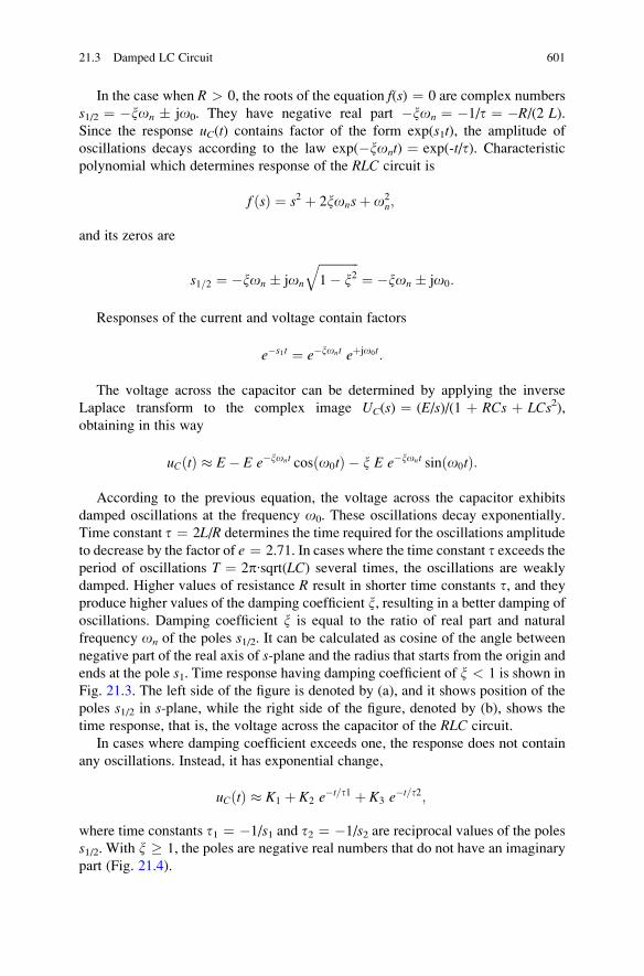
In the case when R > 0, the roots of the equation f(s) ¼ 0 are complex numbers
s1/2 ¼ �xon � jo0. They have negative real part �xon ¼ �1/t ¼ �R/(2 L).Since the response uC(t) contains factor of the form exp(s1t), the amplitude of
oscillations decays according to the law exp(�xont) ¼ exp(-t/t). Characteristicpolynomial which determines response of the RLC circuit is
f ðsÞ ¼ s2 þ 2xonsþ o2n;
and its zeros are
s1=2 ¼ �xon � jon
ffiffiffiffiffiffiffiffiffiffiffiffiffi1� x2
q¼ �xon � jo0:
Responses of the current and voltage contain factors
e�s1t ¼ e�xont eþjo0t:
The voltage across the capacitor can be determined by applying the inverse
Laplace transform to the complex image UC(s) ¼ (E/s)/(1 þ RCs þ LCs2),obtaining in this way
uCðtÞ � E� E e�xont cos o0tð Þ � x E e�xont sin o0tð Þ:
According to the previous equation, the voltage across the capacitor exhibits
damped oscillations at the frequency o0. These oscillations decay exponentially.
Time constant t ¼ 2L/R determines the time required for the oscillations amplitude
to decrease by the factor of e ¼ 2.71. In cases where the time constant t exceeds theperiod of oscillations T ¼ 2p∙sqrt(LC) several times, the oscillations are weakly
damped. Higher values of resistance R result in shorter time constants t, and they
produce higher values of the damping coefficient x, resulting in a better damping of
oscillations. Damping coefficient x is equal to the ratio of real part and natural
frequency on of the poles s1/2. It can be calculated as cosine of the angle between
negative part of the real axis of s-plane and the radius that starts from the origin and
ends at the pole s1. Time response having damping coefficient of x < 1 is shown in
Fig. 21.3. The left side of the figure is denoted by (a), and it shows position of the
poles s1/2 in s-plane, while the right side of the figure, denoted by (b), shows the
time response, that is, the voltage across the capacitor of the RLC circuit.
In cases where damping coefficient exceeds one, the response does not contain
any oscillations. Instead, it has exponential change,
uCðtÞ � K1 þ K2 e�t=t1 þ K3 e
�t=t2;
where time constants t1 ¼ �1/s1 and t2 ¼ �1/s2 are reciprocal values of the poless1/2. With x � 1, the poles are negative real numbers that do not have an imaginary
part (Fig. 21.4).
21.3 Damped LC Circuit 601
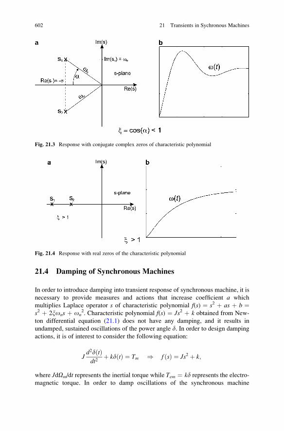
21.4 Damping of Synchronous Machines
In order to introduce damping into transient response of synchronous machine, it is
necessary to provide measures and actions that increase coefficient a which
multiplies Laplace operator s of characteristic polynomial f(s) ¼ s2 þ as þ b ¼s2 þ 2xons þ on
2. Characteristic polynomial f(s) ¼ Js2 þ k obtained from New-
ton differential equation (21.1) does not have any damping, and it results in
undamped, sustained oscillations of the power angle d. In order to design damping
actions, it is of interest to consider the following equation:
Jd2dðtÞdt2
þ kdðtÞ ¼ Tm ) f ðsÞ ¼ Js2 þ k;
where JdOm/dt represents the inertial torque while Tem ¼ kd represents the electro-magnetic torque. In order to damp oscillations of the synchronous machine
Fig. 21.3 Response with conjugate complex zeros of characteristic polynomial
Fig. 21.4 Response with real zeros of the characteristic polynomial
602 21 Transients in Sychronous Machines
connected to a stiff network, it is necessary to extend the above differential equation
by adding the torque component proportional to the first derivative of the power
angle, kP∙dd/dt. This adds the factor kP∙s into characteristic polynomial f(s):
Jd2dðtÞdt2
þ kPddðtÞdt
þ kdðtÞ ¼ Tm ) f ðsÞ ¼ Js2 þ kPsþ k:
Having in mind that characteristic polynomial with two conjugate complex zero
has the form
f ðsÞ ¼ s2 þ 2xonsþ o2n;
the torque component kP∙dd/dt contributes to damping x ¼ kP/(2Jon). The required
torque component can be achieved by introducing small variations of the load
torque. With Tm(t) ¼ Tm0 � kP dd/dt, it is possible to obtain a stable, well-damped
response of the power angle d and the electromagnetic torque of the synchronous
machine. Yet, it is very difficult to make such changes of the torque Tm. Insynchronous generators, the torque TT ¼ �Tm is provided by the steam or water
turbines, which cannot be controlled with desired dynamics. Synchronous motors
are loaded by the torque Tm of respective mechanical loads and work machines.
Neither this torque can include the component kP dd/dt.Damping torque kP dd/dt can be obtained from the very synchronous machine,
provided that the electromagnetic torque Tem included two components, where the
first is proportional to sin(d) ~ d while the second is proportional to the first time
derivative of the power angle, dd/dt. Desired variation of the torque is determined
by expression Tem ¼ kd þ kP dd/dt.Electromagnetic torque of an AC machine depends on the flux and also on the
stator current. On the other hand, the stator current can be changed by altering the
stator voltages. Therefore, generally speaking, desired variation of electromagnetic
torque can be achieved by changing the stator voltages. With changes in stator
voltages determined by dd/dt, the stator currents and the electromagnetic torque
would exhibit changes that depend on dd/dt. However, the subject of this analysis isa synchronous machine connected to a stiff network, where the voltages cannot
change according to dd/dt. Instead, the stator voltages have amplitude and fre-
quency that do not change. Therefore, the damping torque DTem ¼ kP dd/dt requiresthe change of the machine construction and introduction of a new set of windings.
21.5 Damper Winding
Considering that dd/dt ¼ oe � om, the required damping torque DTem ¼ kP dd/dtis proportional to the slip Oe � Om. At steady state, synchronous speed Oe is equal
to the rotor speed Om. During transients caused by the load torque disturbances, the
21.5 Damper Winding 603
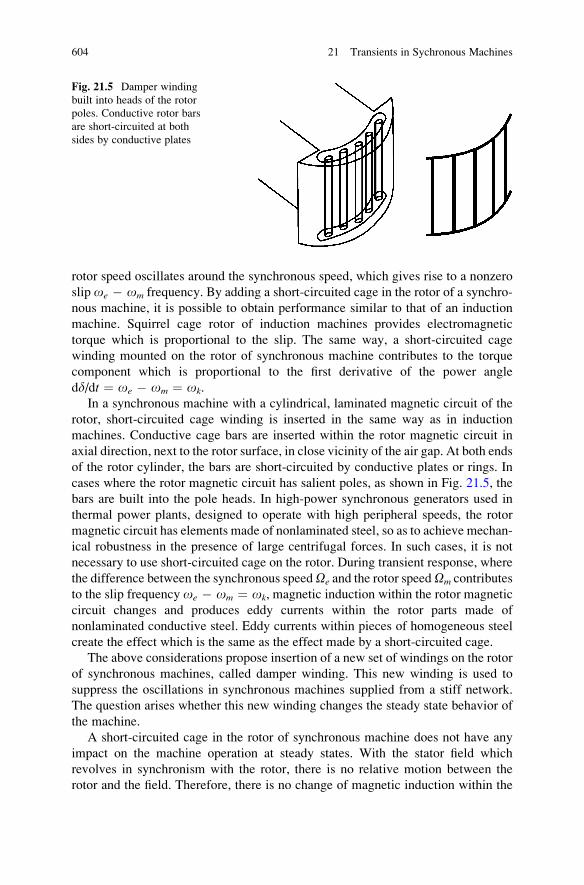
rotor speed oscillates around the synchronous speed, which gives rise to a nonzero
slip oe � om frequency. By adding a short-circuited cage in the rotor of a synchro-
nous machine, it is possible to obtain performance similar to that of an induction
machine. Squirrel cage rotor of induction machines provides electromagnetic
torque which is proportional to the slip. The same way, a short-circuited cage
winding mounted on the rotor of synchronous machine contributes to the torque
component which is proportional to the first derivative of the power angle
dd/dt ¼ oe � om ¼ ok.
In a synchronous machine with a cylindrical, laminated magnetic circuit of the
rotor, short-circuited cage winding is inserted in the same way as in induction
machines. Conductive cage bars are inserted within the rotor magnetic circuit in
axial direction, next to the rotor surface, in close vicinity of the air gap. At both ends
of the rotor cylinder, the bars are short-circuited by conductive plates or rings. In
cases where the rotor magnetic circuit has salient poles, as shown in Fig. 21.5, the
bars are built into the pole heads. In high-power synchronous generators used in
thermal power plants, designed to operate with high peripheral speeds, the rotor
magnetic circuit has elements made of nonlaminated steel, so as to achieve mechan-
ical robustness in the presence of large centrifugal forces. In such cases, it is not
necessary to use short-circuited cage on the rotor. During transient response, where
the difference between the synchronous speedOe and the rotor speedOm contributes
to the slip frequency oe � om ¼ ok, magnetic induction within the rotor magnetic
circuit changes and produces eddy currents within the rotor parts made of
nonlaminated conductive steel. Eddy currents within pieces of homogeneous steel
create the effect which is the same as the effect made by a short-circuited cage.
The above considerations propose insertion of a new set of windings on the rotor
of synchronous machines, called damper winding. This new winding is used to
suppress the oscillations in synchronous machines supplied from a stiff network.
The question arises whether this new winding changes the steady state behavior of
the machine.
A short-circuited cage in the rotor of synchronous machine does not have any
impact on the machine operation at steady states. With the stator field which
revolves in synchronism with the rotor, there is no relative motion between the
rotor and the field. Therefore, there is no change of magnetic induction within the
Fig. 21.5 Damper winding
built into heads of the rotor
poles. Conductive rotor bars
are short-circuited at both
sides by conductive plates
604 21 Transients in Sychronous Machines
rotor magnetic circuit. For this reason, the flux of short-circuited cage winding does
not change, and it produces no electromotive forces. Consequently, there are no
electrical currents within the cage windings, and no change in the torque and flux.
Hence, the machine operates in the same way as it would perform without the cage
winding. During transient processes, where the rotor moves relative to the stator
field, the first derivative of the power angle is equal tooe � om ¼ ok 6¼ 0. For that
reason, the flux within the cage winding changes, and it produces electromotive
forces which depend on the slip ok. This electromotive force produces electrical
currents in short-circuited cage. The angular frequency of these currents is equal to
dd/dt ¼ ok. Through the interaction with the magnetic field, the cage currents
contribute to electromagnetic torque which is proportional to the slip, DTem ¼kP dd/dt. This torque does not exist in steady state conditions. The torque DTemhas stabilizing effects, and it contributes to decay of oscillations in synchronous
machines supplied from stiff networks.
21.6 Short Circuit of Synchronous Machines
Large power synchronous generators used in hydro power plants or thermal power
plants have the rated power from several tens to several hundreds of MW. The line
voltages across the stator windings range from 6 up to 25 kV. In most cases, each
generator has its own power transformer, called block transformer. The stator
terminals are connected to the primary winding of this power transformer. The
transformer has secondary voltages ranging from 110 up to 700 kV. The secondary
winding is connected to the three-phase high-voltage transmission network. The
network extends and reaches large cities and industrial areas, where the high voltage
is supplied to a set of power transformers which reduce the voltage. Following that,
distribution networks feed the electrical energy to individual consumers.
Electrical power system comprises electrical generators, transmission lines, power
transformers, distribution lines, and also various consumers. It has large size and
spreads throughoutwhole countries. Consequently, there are quite frequent faults such
as short circuit, caused by component failures, weather conditions, human error, and
other reasons. Electrical power systems include a sophisticated protection system
which detects the short-circuit faults, interrupts the short-circuit currents, and isolates
the faulty part of the network. Proper functionality of said protection system relies on
synchronous generators supplying the short-circuit current, so as to enable
distinguishing the short-circuit event, its type, and location. For that reason, it is of
interest to study behavior of synchronous machines brought into short circuit.
When a short circuit occurs on the high-voltage transmission line, next to the
power plant, the short-circuit current which is fed from synchronous generator is
directly proportional to the stator electromotive force and inversely proportional to
the equivalent short-circuit impedance. The latter depends on the series impedance
of the high-voltage transmission line, on the series impedance of the block trans-
former, and on the internal impedance of the generator windings.
21.6 Short Circuit of Synchronous Machines 605
In a synchronous generator with constant excitation current, and with negligible
resistance RS, the short-circuit current can be determined from the steady state
equivalent circuit in Fig. 20.1. It is obtained by dividing the electromotive force
E0 and the series reactance XS ¼ oeLS. Excitation winding of large synchronous
generators is supplied from controllable sources of DC voltage which have a finite
output impedance. Therefore, during the short-circuit transients, the assumption
iR ¼ IR ¼ const. does not hold. Moreover, large synchronous generators also
have sets of damper windings. The presence of damper windings in the rotor of
synchronous generator reduces its equivalent impedances and increases the short-
circuit current. More exact calculation of the short-circuit current requires the
model of synchronous machine to be extended by including short-circuited
damper windings.
In Chap. 15, it is shown that the short-circuited cage winding can be modeled by
a system of two orthogonal short-circuited rotor windings. Complete model of
synchronous machine with damper windings comprises five coupled windings.
These five windings are (1) the excitation winding, (2) the stator winding of
d-axis, (3) the stator winding of q-axis, (4) short-circuited damper winding in
d-axis, and (5) short-circuited damper winding in q-axis. The use of complete
model with five coupled windings allows more precise prediction of short-circuit
currents in the stator winding. This model is relatively complex, and it is not
developed nor used in this chapter. Instead, an approximate calculation of the
short-circuit current is proposed which takes into account the impact of the excita-
tion winding and the impact of the damper winding.
When a short circuit occurs at terminals of the stator winding, the stator voltage
drops to US ¼ 0. In an actual short-circuit condition across the high-voltage
transmission line, the stator voltage is not equal to zero. There is a certain series
impedance Z1 between the stator terminals and the short-circuit location. The
analysis of this condition can be simplified by adding the impedance Z1 to the
stator impedance and considering that US ¼ 0. This means that the reactance and
resistance of the stator winding are to be increased by the amount corresponding to
the equivalent series reactance and series resistance between the machine terminals
and the short-circuit site. In further considerations, it will be assumed that the
external inductance and resistance which separate the machine from the short-
circuit site are included in the inductance and resistance of the stator winding.
With that in mind, further analysis is carried out assuming that the stator winding is
short-circuited (US ¼ 0), even in cases where the short circuit occurs along the
high-voltage transmission line.
The subsequent analysis of short circuits is carried out under assumption that the
stator current before the fault is equal to zero. In addition, stator resistance RS in
high-power machines can be neglected; thus, the voltage balance equations take
the form
udq ¼ RSidq þ dCdq=dtþ jomCdq;
) us ¼ 0 ¼ dCdq=dtþ jomCdq: (21.2)
606 21 Transients in Sychronous Machines
Transient processes in a short-circuited synchronous machine include variations
of the flux components in d- and q-axes. Therefore, it is not justified to assume that
the machine operates in the steady state, where the first derivatives of the flux
components in dq coordinate frame are equal to zero. On the other hand, complete
mathematical model of synchronous machine with stator windings, excitation
winding, and damper windings is rather complex. In order to obtain an estimate
of shortcircuit currents, it is of interest to simplify the analysis by introducing
certain approximations. These approximations are based on the fact that the time
constants that characterize transient processes in damping cage windings decay
quickly, while transient processes in excitation winding last longer. Therefore, the
short-circuit process is split in three intervals:
• Subtransient interval, where transient processes in damping cage have not ceased
and where the damping cage current contributes to the short-circuit current.
• Transient interval that follows subtransient interval and starts after the damping
cage currents has decayed to zero.
• Steady state interval, which follows after the transient phenomena in both
damping and excitation winding have ceased and where the short-circuit current
can be determined from the steady state equivalent circuit in Fig. 20.1.
21.6.1 DC Component
The steady state operation of electrical circuits with AC currents and voltages can
be disturbed by stepwise changes of voltage or current sources, by changing the
circuit impedance, or by introducing short circuits or open circuits. Whenever such
transients occur, the process of passing from the previous steady state condition into
a new steady state condition may involve a certain amount of DC current that exists
during transients and that decays as the circuit enters the new steady state condition.
Well-known example involves connecting the coil of the self-inductance L to a
voltage source uL(t) ¼ Um sin(ot) at instant t ¼ 0, where iL(0) ¼ 0. The coil
current for t > 0 is equal to iL(t) ¼ (Um/L/o)∙(1 � cos(ot)), and it contains a DC
component. In coils with a finite resistance R, this DC current decays with the time
constant of t ¼ L/R. Similar processes take place in short-circuited synchronous
machines.
During short circuit of the stator winding, the phase voltages are equal to zero.
Therefore, the voltage balance equation in phase a is ua ¼ 0 ¼ RSia þ dCa/dt. Inlarge synchronous machine, the voltage drop RSia is very small. Therefore, equation
reduces to dCa/dt ¼ 0, meaning that the flux in each phase tends to retain the value
Ca(0�) which corresponds to the flux at the instant of making the short circuit.
Therefore, it is assumed that the flux in short-circuited windings remains constant
during the short-circuit fault. Even large power synchronous machines have a finite
value of the stator resistance RS > 0. Although very small, the voltage RSiadoes influence the winding flux, in particular, over longer intervals of time.
21.6 Short Circuit of Synchronous Machines 607
Considering that the short circuits are of limited duration, the assumption dCa/
dt ¼ 0 can be successfully used to facilitate calculation of short-circuit currents.
During steady state operation before the short circuit, the flux in phase a varies assinusoidal function of the frequency om ¼ oe. The average value of the flux Ca
prior to the short circuit is equal to zero. At the instant of the short circuit, the value
of flux is Ca ¼ Ca(0�). If the voltage drop RSia is negligible, the flux in phase a
retains the value Ca(0�) during the short-circuit conditions. Therefore, flux Ca
comprises a DC component. Due to the presence of a small but finite voltage drop
RSia, the DC component of the flux exponentially decays. The time constant t ¼LgeS/RS determines the rate of change of the DC component, and it depends on the
equivalent inductance LgeS and the stator resistance RS. Larger values of the winding
resistance result in quicker decay of DC component. Detailed analysis of changes in
the machine torque, speed, and ab and dq variables that are caused by the DC
component of the stator flux requires evaluation of the complete mathematical
model. This model includes the damping cage windings, and it is rather involved
and difficult to evaluate. Therefore, further considerations are based on the assump-
tion that the time constant t ¼ LgeS/RS is relatively small and that the DC
components of the stator flux decay rather quickly. With DC component decay
time significantly shorter than the duration of the short-circuit phenomena, it is
possible to neglect the DC component and to assume that the initial value of the flux
is equal to zero. With that in mind, the initial value of the phase flux linkages at the
short-circuit instant is given by equations Ca(0+) ¼ Cb(0
+) ¼ Cc(0+) ¼ 0, which
results in Cd(0+) ¼ Cq(0
+) ¼ 0.
The purpose of this discussion is to obtain an approximate change of the short-
circuit current. The analysis is simplified by the assumption that Cd(0+) ¼ Cq(0
+)
¼ 0. The assumption will be used in calculating the short-circuit current ISC.The short-circuit current is affected by the value of the excitation current IR at
the instant of the short circuit and on the values of the stator currents at the same
instant. The short-circuit current of synchronous machine that was running with no
load prior to the fault is different than the short-circuit current of loaded machine. In
order to keep the analysis simple, the subsequent steps consider the situation where
the short circuit occurs while the machine is not loaded. Hence, the stator currents
are equal to zero in the wake of the short circuit, resulting in id(0�) ¼ 0 and
iq(0�) ¼ 0. Notwithstanding the abovementioned assumptions, the subsequent
analysis helps the reader understand the basic intervals of short-circuit transients,
and it also provides the means to obtain a rough estimate of the short-circuit
currents in each interval:
• During subtransient interval, both the damping cage and the excitation winding
contribute to short-circuit current ISC3.• In the following transient interval, the cage currents have ceased, and the short-
circuit current ISC2 is aided by the excitation winding.
• Steady state short-circuit current ISC1 is calculated assuming that transient
processes in the excitation winding have ended and that the excitation current
IR is constant.
608 21 Transients in Sychronous Machines
Within the subsequent considerations, the short-circuit current ISC1 is calculatedfirst, assuming that the excitation current iR(t) ¼ IR does not change. In calculationof ISC1, it is justifiable to consider that the excitation winding is supplied from a
current source and that the machine does not have damping cage.
Then, the short-circuit current ISC2 is calculated, considering transient phenom-
ena in the excitation winding which is supplied from the voltage source.
Finally, the short-circuit current ISC3 is calculated by taking into account the
impact of transient processes in damping cage and transient processes in excitation
winding on the current in short-circuited stator windings.
21.6.2 Calculation of ISC1
It is of interest to calculate the short-circuit current ISC1 which exists in the stator
windings when the transient processes in other windings have decayed and when
the excitation current iR(t) ¼ IR does not change. In this calculation, it is justifiableto assume that the damper winding does not exist and that the excitation winding is
supplied from the current source.2 Considering condition Cd ¼ Cq ¼ 0, relations
Lqiq ¼ 0 and Ldid þ LmIP ¼ 0 are obtained for a synchronous machine which does
not have damper windings.3 Components of the current ISC1 are given by (21.3),
where E0 represents the no load electromotive force obtained with the excitation
current IR:
iq ¼ 0;
id ¼ � LmIRLd
¼ �omLmIRomLd
¼ �omLmIRomLd
¼ �E0
Xd:
ISC1 ¼ E0
Xd(21.3)
Therefore, the rms value of the short-circuit current is 0.707∙ISC1 ¼ 0.707E0/Xd.
When the short-circuit fault persists, the current ISC1 does not decay in time, and it
is retained in the stator winding until the short circuit is disconnected. Instantaneous
values of the corresponding phase currents can be obtained by applying the inverse
Park and inverse 3F/2F transform to the components obtained in (21.3).
2 Excitation windings of large synchronous machines are supplied from adjustable sources of DC
voltage. The source voltage is used as the driving force which is used to control the excitation
current. At the wake of the short circuit event, the changes in the excitation voltage can be
neglected, and it is justifiable to assume that the excitation winding is supplied from the voltage
source that provides a constant voltage. Later on, as the transient phenomena decay while the short
circuit persists, it is justifiable to assume that the excitation current is constant, namely, that the
excitation winding is supplied from a source of constant current.3 In the considered case, the machine is equipped by damper windings, but the transient processes
in these windings have ceased, and the electrical currents in damper windings are equal to zero.
21.6 Short Circuit of Synchronous Machines 609
21.6.3 Calculation of ISC2
The excitation winding of large synchronous machines is supplied either from an
auxiliary DC generator, which provides adjustable excitation voltage and which is
called exciter, or from a static power converter with large thyristors, which converts
the three-phase AC voltages into adjustable DC voltage. Both the exciter machine
and the static power converter can be modeled as a DC voltage source which
provides adjustable voltage, and which has a finite, relatively low internal resistance.
The excitation voltage is adjusted by the excitation controller. As the shortcircuit
takes place all of a sudden, the excitation voltage remains constant for a while,
and it retains the value UR ¼ RRIR that existed before the short circuit. Notice that
IR denotes the value of the excitation current prior to the short circuit, while iR(t)denotes the change of the excitation current during the transients.
The excitation winding is magnetically coupled to the stator winding, which is
short-circuited. Due to a finite mutual inductance between the stator windings and
the excitation winding, the short-circuit stator currents affect the mutual flux. With
the excitation winding supplied from a voltage source, these changes introduce
variation in the excitation current. Assuming that the voltage drop UR ¼ RRIRacross the resistance of the excitation winding is relatively small, the voltage
balance equation for the excitation winding reduces to the expression dCR/
dt ¼ 0. Therefore, with excitation winding supplied from the voltage source, and
with RRIR � 0, the flux CR ¼ LRiR þ Lmid retains the value LRIR which existed
prior to the short-circuit fault.
On the bases of the previous considerations, the stator flux components maintain
the valuesCd(0+) ¼ Cq(0
+) ¼ 0 throughout the short-circuit transients. One part of
the stator flux encircles the excitation winding. The axis d of synchronous dq frame
coincides with magnetic axis of the excitation winding. Therefore, condition
Cd(0+) ¼ 0 reduces the flux in the excitation winding. Variation of the flux in the
excitation winding causes induction of an electromotive force which acts toward
increasing the excitation current iR(t), in an attempt to suppress the reduction in the
excitation flux and to maintain the flux linkage that existed prior to the short circuit.
Neglecting the voltage drop RRiR in the voltage balance equation for the excitation
winding, it is reasonable to assume that the relation dCR/dt � 0 holds for relatively
short intervals of time. With that in mind, the excitation flux CR tends to retain the
value CR0 that existed prior to the short-circuit fault. Therefore,
Lqiq ¼ 0; ) iq ¼ 0;
CR ¼ LRiR þ Lmid ¼ CR0 ¼ LRIR; ) iR ¼ IR0 � LmLR
id;
Cd ¼ Ldid þ LmiR ¼ 0 ¼ Ldid þ LmIR0 � L2mLR
id:
(21.4)
610 21 Transients in Sychronous Machines
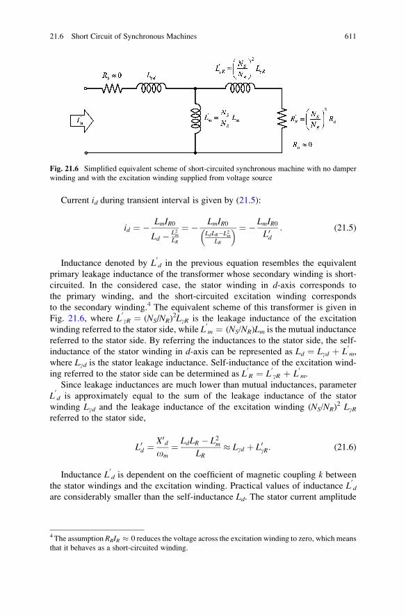
Current id during transient interval is given by (21.5):
id ¼ � LmIR0
Ld � L2mLR
¼ � LmIR0LdLR�L2m
LR
� � ¼ � LmIR0L0d
: (21.5)
Inductance denoted by L0d in the previous equation resembles the equivalent
primary leakage inductance of the transformer whose secondary winding is short-
circuited. In the considered case, the stator winding in d-axis corresponds to
the primary winding, and the short-circuited excitation winding corresponds
to the secondary winding.4 The equivalent scheme of this transformer is given in
Fig. 21.6, where L0gR ¼ (NS/NR)
2LgR is the leakage inductance of the excitation
winding referred to the stator side, while L0m ¼ (NS/NR)Lm is the mutual inductance
referred to the stator side. By referring the inductances to the stator side, the self-
inductance of the stator winding in d-axis can be represented as Ld ¼ Lgd þ L0m,
where Lgd is the stator leakage inductance. Self-inductance of the excitation wind-
ing referred to the stator side can be determined as L0R ¼ L
0gR þ L
0m.
Since leakage inductances are much lower than mutual inductances, parameter
L0d is approximately equal to the sum of the leakage inductance of the stator
winding Lgd and the leakage inductance of the excitation winding (NS/NR)2 LgR
referred to the stator side,
L0d ¼X0
d
om¼ LdLR � L2m
LR� Lgd þ L0gR: (21.6)
Inductance L0d is dependent on the coefficient of magnetic coupling k between
the stator windings and the excitation winding. Practical values of inductance L0d
are considerably smaller than the self-inductance Ld. The stator current amplitude
Fig. 21.6 Simplified equivalent scheme of short-circuited synchronous machine with no damper
winding and with the excitation winding supplied from voltage source
4 The assumption RRIR � 0 reduces the voltage across the excitation winding to zero, which means
that it behaves as a short-circuited winding.
21.6 Short Circuit of Synchronous Machines 611
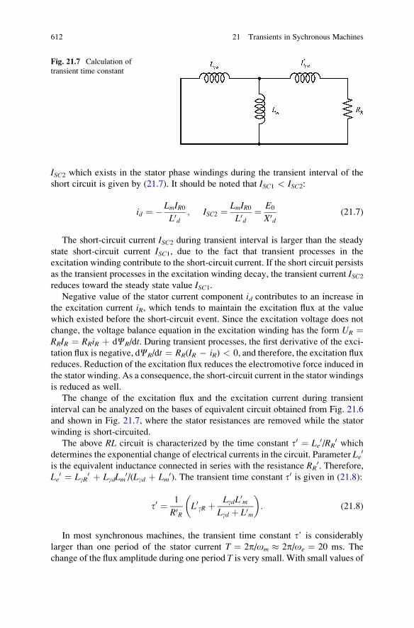
ISC2 which exists in the stator phase windings during the transient interval of the
short circuit is given by (21.7). It should be noted that ISC1 < ISC2:
id ¼ � LmIR0L0d
; ISC2 ¼ LmIR0L0d
¼ E0
X0d
(21.7)
The short-circuit current ISC2 during transient interval is larger than the steady
state short-circuit current ISC1, due to the fact that transient processes in the
excitation winding contribute to the short-circuit current. If the short circuit persists
as the transient processes in the excitation winding decay, the transient current ISC2reduces toward the steady state value ISC1.
Negative value of the stator current component id contributes to an increase in
the excitation current iR, which tends to maintain the excitation flux at the value
which existed before the short-circuit event. Since the excitation voltage does not
change, the voltage balance equation in the excitation winding has the form UR ¼RRIR ¼ RRiR þ dCR/dt. During transient processes, the first derivative of the exci-
tation flux is negative, dCR/dt ¼ RR(IR � iR) < 0, and therefore, the excitation flux
reduces. Reduction of the excitation flux reduces the electromotive force induced in
the stator winding. As a consequence, the short-circuit current in the stator windings
is reduced as well.
The change of the excitation flux and the excitation current during transient
interval can be analyzed on the bases of equivalent circuit obtained from Fig. 21.6
and shown in Fig. 21.7, where the stator resistances are removed while the stator
winding is short-circuited.
The above RL circuit is characterized by the time constant t0 ¼ Le0/RR
0 whichdetermines the exponential change of electrical currents in the circuit. Parameter Le
0
is the equivalent inductance connected in series with the resistance RR0. Therefore,
Le0 ¼ LgR
0 þ LgdLm0/(Lgd þ Lm
0). The transient time constant t0 is given in (21.8):
t0 ¼ 1
R0R
L0gR þ LgdL0m
Lgd þ L0m
� �: (21.8)
In most synchronous machines, the transient time constant t’ is considerably
larger than one period of the stator current T ¼ 2p/om � 2p/oe ¼ 20 ms. The
change of the flux amplitude during one period T is very small. With small values of
Fig. 21.7 Calculation of
transient time constant
612 21 Transients in Sychronous Machines
T/t0, exponential decay within one period of stator currents can be approximated by
the expression exp(�T/t0) � 1 � T/t0 � 1. The stator currents during short circuit
can be regarded as sinusoidal, with an amplitude that decays exponentially.
From the previous analysis, it is possible to obtain the change of the short-circuit
current in a synchronous machine with no damping cage winding and with voltage-
supplied excitation winding. In absence of the damper windings, the short-circuit
phenomena do not have subtransient interval. During the transient interval, imme-
diately upon the short circuits is established, the amplitude of the stator phase
current is ISC2 (21.7). It decays exponentially and reaches the steady state value
ISC1. The change of the current amplitude is determined by the time constant t’. Theactual change of the phase current ia(t) depends on the initial phase of the stator
voltages prior to the short circuit, on the instant of establishing the short circuit, and
also on the circuit resistances that have been neglected. As an example, the phase
current ia(t) may change as
iaðtÞ � ISC1 þ ISC2 � ISC1ð Þ � exp � t
t0� �n o
sin omtþ ’að Þ:
The analysis performed above takes into account dynamic phenomena in d-axis.In the considered case, the currents and fluxes in q-axis were equal to zero prior to theshort circuit. The accuracy in calculating the short-circuit currents can be further
enhanced by taking into account the coupling of transient processes d-axis and
q-axis. The coupling between transient phenomena in orthogonal axes can be
understood from differential equations expressing the voltage balance in virtual
d-winding and q-winding. It has to be noted at this point that the q-axis does not havemagnetic coupling with the excitation winding. The rotor of synchronous machines
comprises only one excitation winding, and this winding has magnetic axis aligned
with d-axis of the dq coordinate frame. For this reason, (21.3) and (21.7) provide an
adequate approximation of the short-circuit current during transient and steady state
intervals.
21.6.4 Calculation of ISC3
The presence of short-circuited damping cage increases the amplitude of the short-
circuit current. Short-circuited windings exhibit the tendency to maintain the flux.
Any flux change results in induced electromotive forces and electrical currents in
short-circuited windings that oppose to the flux change and act toward retaining the
flux at the previous level. While the short-circuit event tends to drive the stator flux
to zero, the damper windings act toward maintaining the flux. With larger flux, the
stator electromotive forces are larger, which results in an increased amplitude of the
short-circuit currents. This effect dies out as the transient processes in the damper
windings cease.
21.6 Short Circuit of Synchronous Machines 613
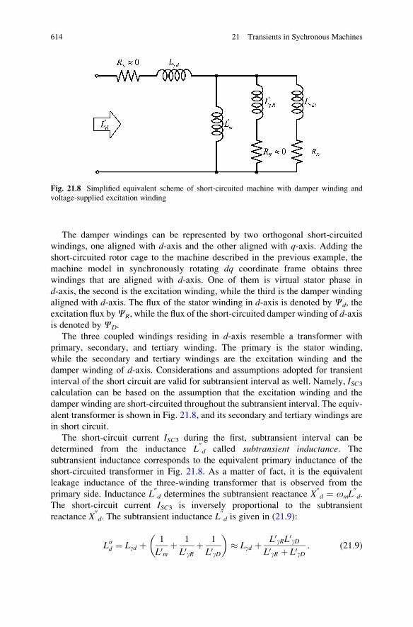
The damper windings can be represented by two orthogonal short-circuited
windings, one aligned with d-axis and the other aligned with q-axis. Adding the
short-circuited rotor cage to the machine described in the previous example, the
machine model in synchronously rotating dq coordinate frame obtains three
windings that are aligned with d-axis. One of them is virtual stator phase in
d-axis, the second is the excitation winding, while the third is the damper winding
aligned with d-axis. The flux of the stator winding in d-axis is denoted by Cd, the
excitation flux byCR, while the flux of the short-circuited damper winding of d-axisis denoted by CD.
The three coupled windings residing in d-axis resemble a transformer with
primary, secondary, and tertiary winding. The primary is the stator winding,
while the secondary and tertiary windings are the excitation winding and the
damper winding of d-axis. Considerations and assumptions adopted for transient
interval of the short circuit are valid for subtransient interval as well. Namely, ISC3calculation can be based on the assumption that the excitation winding and the
damper winding are short-circuited throughout the subtransient interval. The equiv-
alent transformer is shown in Fig. 21.8, and its secondary and tertiary windings are
in short circuit.
The short-circuit current ISC3 during the first, subtransient interval can be
determined from the inductance L00d called subtransient inductance. The
subtransient inductance corresponds to the equivalent primary inductance of the
short-circuited transformer in Fig. 21.8. As a matter of fact, it is the equivalent
leakage inductance of the three-winding transformer that is observed from the
primary side. Inductance L00d determines the subtransient reactance X
00d ¼ omL
00d.
The short-circuit current ISC3 is inversely proportional to the subtransient
reactance X00d. The subtransient inductance L
00d is given in (21.9):
L00d ¼ Lgd þ 1
L0mþ 1
L0gRþ 1
L0gD
� �� Lgd þ L0gRL0gD
L0gR þ L0gD: (21.9)
Fig. 21.8 Simplified equivalent scheme of short-circuited machine with damper winding and
voltage-supplied excitation winding
614 21 Transients in Sychronous Machines
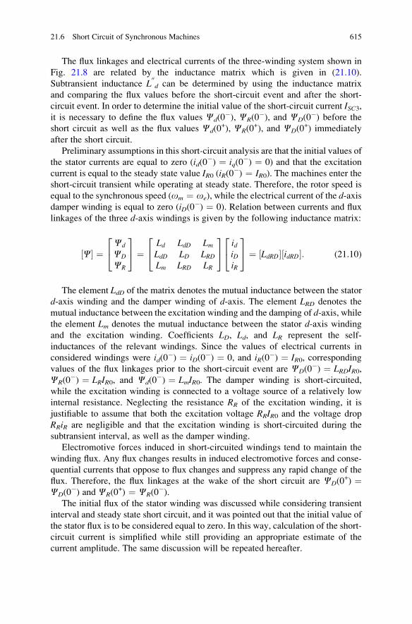
The flux linkages and electrical currents of the three-winding system shown in
Fig. 21.8 are related by the inductance matrix which is given in (21.10).
Subtransient inductance L00d can be determined by using the inductance matrix
and comparing the flux values before the short-circuit event and after the short-
circuit event. In order to determine the initial value of the short-circuit current ISC3,it is necessary to define the flux values Cd(0
�), CR(0�), and CD(0
�) before the
short circuit as well as the flux values Cd(0+), CR(0
+), and CD(0+) immediately
after the short circuit.
Preliminary assumptions in this short-circuit analysis are that the initial values of
the stator currents are equal to zero (id(0�) ¼ iq(0
�) ¼ 0) and that the excitation
current is equal to the steady state value IR0 (iR(0�) ¼ IR0). The machines enter the
short-circuit transient while operating at steady state. Therefore, the rotor speed is
equal to the synchronous speed (om ¼ oe), while the electrical current of the d-axisdamper winding is equal to zero (iD(0
�) ¼ 0). Relation between currents and flux
linkages of the three d-axis windings is given by the following inductance matrix:
C½ � ¼Cd
CD
CR
24
35 ¼
Ld LdD LmLdD LD LRDLm LRD LR
24
35 id
iDiR
24
35 ¼ LdRD½ � idRD½ �: (21.10)
The element LdD of the matrix denotes the mutual inductance between the stator
d-axis winding and the damper winding of d-axis. The element LRD denotes the
mutual inductance between the excitation winding and the damping of d-axis, whilethe element Lm denotes the mutual inductance between the stator d-axis windingand the excitation winding. Coefficients LD, Ld, and LR represent the self-
inductances of the relevant windings. Since the values of electrical currents in
considered windings were id(0�) ¼ iD(0
�) ¼ 0, and iR(0�) ¼ IR0, corresponding
values of the flux linkages prior to the short-circuit event are CD(0�) ¼ LRDIR0,
CR(0�) ¼ LRIR0, and Cd(0
�) ¼ LmIR0. The damper winding is short-circuited,
while the excitation winding is connected to a voltage source of a relatively low
internal resistance. Neglecting the resistance RR of the excitation winding, it is
justifiable to assume that both the excitation voltage RRIR0 and the voltage drop
RRiR are negligible and that the excitation winding is short-circuited during the
subtransient interval, as well as the damper winding.
Electromotive forces induced in short-circuited windings tend to maintain the
winding flux. Any flux changes results in induced electromotive forces and conse-
quential currents that oppose to flux changes and suppress any rapid change of the
flux. Therefore, the flux linkages at the wake of the short circuit are CD(0+) ¼
CD(0�) and CR(0
+) ¼ CR(0�).
The initial flux of the stator winding was discussed while considering transient
interval and steady state short circuit, and it was pointed out that the initial value of
the stator flux is to be considered equal to zero. In this way, calculation of the short-
circuit current is simplified while still providing an appropriate estimate of the
current amplitude. The same discussion will be repeated hereafter.
21.6 Short Circuit of Synchronous Machines 615
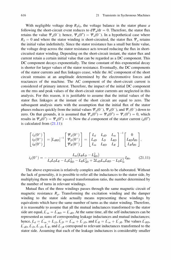
With negligible voltage drop RSiS, the voltage balance in the stator phase afollowing the short-circuit event reduces to dCa/dt ¼ 0. Therefore, the stator flux
retains the value Ca(0�); hence, Ca(0
+) ¼ Ca(0�). In a hypothetical case where
RS ¼ 0 and where the stator winding is short-circuited, the stator flux Ca retains
the initial value indefinitely. Since the stator resistance has a small but finite value,
the voltage drop across the stator resistance acts toward reducing the flux in short-
circuited stator winding. Depending on the short-circuit instant, the stator flux and
current retain a certain initial value that can be regarded as a DC component. This
DC component decays exponentially. The time constant of this exponential decay
is shorter for larger values of the stator resistance. Eventually, the DC components
of the stator currents and flux linkages cease, while the AC component of the short
circuit remains at an amplitude determined by the electromotive forces and
reactances of the machine. The AC component of the short-circuit current is
considered of primary interest. Therefore, the impact of the initial DC component
on the rms and peak values of the short-circuit stator currents are neglected in this
analysis. For this reason, it is justifiable to assume that the initial values of the
stator flux linkages at the instant of the short circuit are equal to zero. The
subsequent analysis starts with the assumption that the initial flux of the stator
phases reduces quickly from the initial valuesCa(0�),Cb(0
�), andCc(0�) down to
zero. On that grounds, it is assumed that Ca(0+) ¼ Cb(0
+) ¼ Cc(0+) ¼ 0, which
results in Cd(0+) ¼ Cq(0
+) ¼ 0. Now the d component of the stator current id(0+)
is calculated from (21.11):
id 0þð ÞiD 0þð ÞiR 0þð Þ
24
35 ¼ LdRD½ ��1
Cd 0þð ÞCD 0þð ÞCR 0þð Þ
24
35 ¼
Ld LdD LmLdD LD LRDLm LRD LR
24
35�1
0
LRDIR0LRIR0
24
35;
id 0þð Þ ¼ � Lm LRLD � L2RD
LdLDLR � LdL2RD � LRL2dD þ 2LdDLmLRD � LDL2mIR0: (21.11)
The above expression is relatively complex and needs to be elaborated. Without
the lack of generality, it is possible to refer all the inductances to the stator side, by
multiplying them with the squared transformation ratio, the number determined by
the number of turns in relevant windings.
Mutual flux of the three windings passes through the same magnetic circuit of
magnetic resistance Rm. Transforming the excitation winding and the damper
winding to the stator side actually means representing these windings by
equivalents which have the same number of turns as the stator winding. Therefore,
it is reasonable to assume that all the mutual inductances transformed to the stator
side are equal, L0m ¼ L
0RD ¼ L
0dD. At the same time, all the self-inductances can be
represented as sums of corresponding leakage inductances and mutual inductances;
hence, Ld ¼ L0m þ LgS, L
0D ¼ L
0m þ L
0gD, and L
0R ¼ L
0m þ L
0gR. The values L
0RD,
L0dD, L
0D, L
0gD, L
0R, and L
0gR correspond to relevant inductances transformed to the
stator side. Assuming that each of the leakage inductances is considerably smaller
616 21 Transients in Sychronous Machines
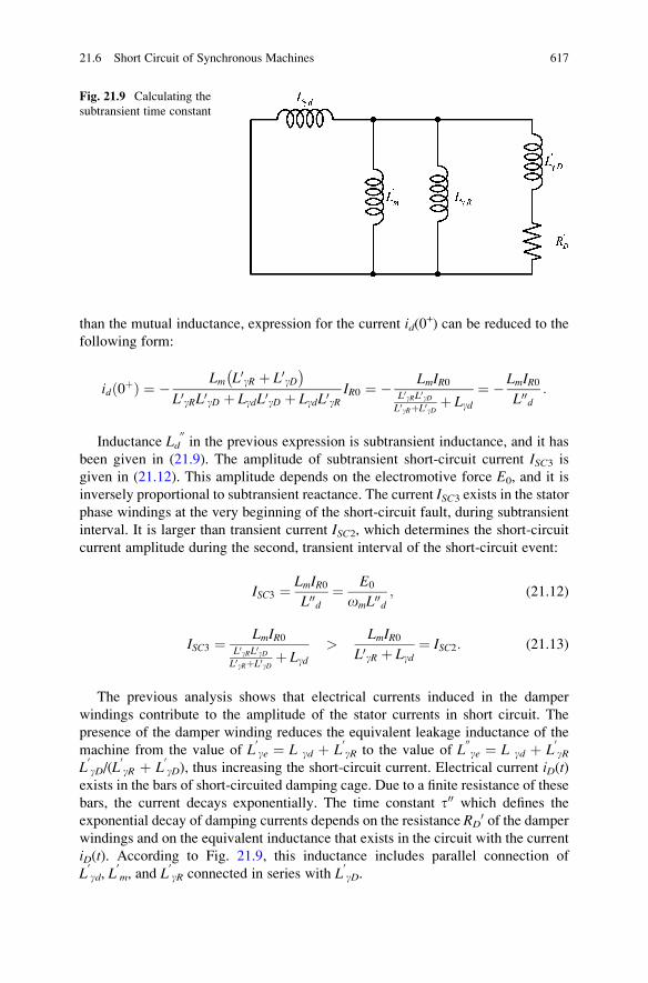
than the mutual inductance, expression for the current id(0+) can be reduced to the
following form:
id 0þð Þ ¼ � Lm L0gR þ L0gD
L0gRL0gD þ LgdL0gD þ LgdL0gRIR0 ¼ � LmIR0
L0gRL0gDL0gRþL0gD
þ Lgd¼ � LmIR0
L00d:
Inductance Ld00in the previous expression is subtransient inductance, and it has
been given in (21.9). The amplitude of subtransient short-circuit current ISC3 is
given in (21.12). This amplitude depends on the electromotive force E0, and it is
inversely proportional to subtransient reactance. The current ISC3 exists in the statorphase windings at the very beginning of the short-circuit fault, during subtransient
interval. It is larger than transient current ISC2, which determines the short-circuit
current amplitude during the second, transient interval of the short-circuit event:
ISC3 ¼ LmIR0L00d
¼ E0
omL00d; (21.12)
ISC3 ¼ LmIR0L0gRL0gDL0gRþL0gD
þ Lgd>
LmIR0L0gR þ Lgd
¼ ISC2: (21.13)
The previous analysis shows that electrical currents induced in the damper
windings contribute to the amplitude of the stator currents in short circuit. The
presence of the damper winding reduces the equivalent leakage inductance of the
machine from the value of L0ge ¼ L gd þ L
0gR to the value of L
00ge ¼ L gd þ L
0gR
L0gD/(L
0gR þ L
0gD), thus increasing the short-circuit current. Electrical current iD(t)
exists in the bars of short-circuited damping cage. Due to a finite resistance of these
bars, the current decays exponentially. The time constant t00 which defines the
exponential decay of damping currents depends on the resistance RD0 of the damper
windings and on the equivalent inductance that exists in the circuit with the current
iD(t). According to Fig. 21.9, this inductance includes parallel connection of
L0gd, L
0m, and L
0gR connected in series with L
0gD.
Fig. 21.9 Calculating the
subtransient time constant
21.6 Short Circuit of Synchronous Machines 617
Based upon Fig. 21.9, subtransient time constant t00 is calculated in (21.14). Thisequation relies on the assumption that the resistance RR of the excitation winding
can be neglected and that the mutual inductance L0m is much larger than the leakage
inductances:
t00 ¼ 1
R0D
LgD þ 1
L0mþ 1
L0gRþ 1
L0gd
� ��1" #
� 1
R0D
LgD þ L0gRL0gdL0gR þ L0gd
� �:
(21.14)
Transferred to the stator side, the damping resistance R0D is larger than the
resistance of the excitation winding. Therefore, the subtransient time constant t00
is shorter than the transient time constant t0. Therefore, the short-circuit event in
synchronous machines has three intervals. It begins with a brief subtransient
interval, proceeds with somewhat longer transient interval, and, unless interrupted,
enters the steady state short-circuit interval. The three intervals are discussed
below.
21.7 Transient and Subtransient Phenomena
21.7.1 Interval 1
The first interval of the short circuit is subtransient interval, which starts immedi-
ately after the instant of establishing the short-circuit conditions. The current of the
amplitude ISC3 is established in the stator windings. This current is directly propor-
tional to the excitation current and inversely proportional to the subtransient
inductance of the machine, denoted by L00d. Subtransient current decays exponen-
tially with the subtransient time constant t00. After several intervals of t00, the currentamplitude reduces to ISC2. At the end of subtransient interval, transient processes indamper winding have decayed, and damping currents have reduced to zero. At this
point, the damper windings cease to make any contribution to short-circuit currents.
21.7.2 Interval 2
During the second interval, called transient interval, the amplitude of short-circuit
currents in the stator windings is ISC2. This current is directly proportional to the
excitation current and inversely proportional to transient inductance of the machine
L0d. The current amplitude decays exponentially with the time constant t0. After
several transient time constant t0, the amplitude of the stator currents reduces to ISC1.
618 21 Transients in Sychronous Machines
At the end of transient interval, transient processes in the excitation winding have
decayed, and the excitation current settles to the steady state value IR0 ¼ UR/RR.
At this point, the excitation winding does not have any transient currents which
contribute to short-circuit currents in the stator windings.
21.7.3 Interval 3
After subtransient and transient interval, transient processes in the excitation
winding and the damper windings decay. Damping currents reduce to zero, while
the excitation current settles on the steady state value. At this point, the short-circuit
current can be determined from the steady state equivalent circuit in Fig. 20.1.
The steady state short-circuit current in the stator winding has amplitude ISC1, whichis directly proportional to the excitation current and inversely proportional to the
stator inductance Ld � Lm. This amplitude does not change until protection
mechanisms are activated to disconnect the stator winding from the short circuit.
Interval 1 is commonly called subtransient interval, and the reactance X00d ¼
omL00d is called subtransient reactance. Interval 2 is called transient interval, while
reactance X0d ¼ omL
0d is called transient reactance. Expressions for the short-
circuit currents in transient and subtransient intervals are obtained by adopting a
series of approximations aimed to simplify calculations and to make the basic short-
circuit behavior more obvious. Expressions such as (21.12, 21.13, and 21.14) are
relatively simple, and they give an insight into the impact of the machine
parameters on the amplitude and dynamic behavior of the short-circuit current.
More precise calculations require solving the complete mathematical model of
synchronous machine which comprises five magnetically coupled windings.
In synchronous generators, practical relative values of synchronous reactance xdrange from 0.8 up to 2. Relative values of transient reactance x
0d range from 0.2 up
to 0.5, while relative values of subtransient reactance range from 0.1 up to 0.3.
Transient time constant t0 has values from 400 ms up to 2 s, while subtransient
interval t00 runs from 30 to 150 ms.
21.7 Transient and Subtransient Phenomena 619
Chapter 22
Variable Frequency Synchronous Machines
This chapter studies the operation and characteristics of three-phase synchronous
machines connected to three-phase inverters, static power converters capable of
adjusting the stator voltages by means of changing the width of the voltage pulses
supplied to the stator terminals. The average voltage of the pulse train is adjusted to
suit the machine needs. Variable speed operation of synchronous machine is
achieved with variable frequency and variable amplitude of stator voltages. This
chapter introduces and explains some basic torque and speed control principles.
The need of controlling the stator currents is discussed and explained. Fundamental
principles of stator current control are introduced, relying on PWM-controlled
three-phase inverter as the voltage actuator. Field-weakening performance of
inverter-supplied synchronous machines with buried magnets and surface-mounted
magnets is analyzed and explained. The limits of constant power operation in field-
weakening mode are determined, explained, and expressed in terms of the stator
self-inductance. Based upon the study of operating limits of the machine and
operating limits of associated three-phase inverter, steady-state operating area
and transient operating area are derived in T � O plane and studied for inverter-
supplied synchronous machines.
22.1 Inverter-Supplied Synchronous Machines
Synchronous machines of low and medium power are used in applications such as
motion control, vehicle propulsion, industrial robots, or production machines.
In these applications, synchronous machines have task to overcome motion resis-
tance and provide the required acceleration and deceleration of moving parts.
Synchronous motor is used as an actuator which develops the torque required to
control the speed or position and to overcome the motion resistances while driving
S.N. Vukosavic, Electrical Machines, Power Electronics and Power Systems,
DOI 10.1007/978-1-4614-0400-2_22, # Springer Science+Business Media New York 2013
621
the controlled object along predefined trajectories. Synchronous motors are better
suited to these tasks than the other electrical motors. Advantages of synchronous
machines over the other types of electrical machines include their high specific
power, high specific torque, a low inertia, and relatively low losses. Synchronous
machines with permanent magnet excitation have no rotor windings and no rotor
losses. Therefore, energy efficiency of these motors is considerably improved
over other types of motors. With permanent magnets, the rotor flux is obtained
without power losses such as URIR ¼ RRIR2, encountered in machines which have
the excitation winding. Moreover, there are no iron losses in the rotor magnetic
circuit of synchronous machine. Due to synchronous rotation of the rotor and the
stator field, there are no pulsations of magnetic induction B in magnetic circuit of
the rotor.
With no rotor losses and no heat generated within the rotor, the cooling of
permanent magnet synchronous machines is greatly simplified, and it is possible
to reach larger current densities in the stator winding and larger magnetic induction,
which results in higher specific power.1 Compared to an induction machine of the
same rated power, synchronous machine with permanent magnets has 20–30%
lower mass and volume. The power balance charts drawn for induction machines
and synchronous machines have the same losses in the stator winding, in the stator
magnetic circuit, and in the mechanical subsystem. Induction machines have power
losses in the rotor which are equal to sPd, where s is relative slip while Pd is the
air-gap power. Synchronous machines do not have the losses sPd, and this greatly
increases their energy efficiency.
In applications suchasmotioncontrol, vehicle propulsion, and industry automation,
it is required to provide continuous change of the rotor speed. In synchronous
machines, the rotor speed corresponds to the synchronous speed Oe ¼ poe, which
is determined by the supply frequency oe. For this reason, synchronous motors in
motion control applications have to be supplied from separate power sources that
produce three-phase voltages of variable frequency and variable amplitude, in
accordance with the motor needs. Two synchronous motors within the same indus-
trial robot or electrical vehicle most often rotate at different rotor speeds. Therefore,
eachmotor has its own supply frequency, and it requires a separate power source that
provides the stator voltages and currents of desired frequency. Such power sources
are usually three-phase inverters with transistor power switches. Commutation of
power transistors produces a train of variable width voltage pulses. The pulse width
of these pulses affects the average voltage within one commutation period.
By sinusoidal change of the pulse width, the average voltage exhibits sinusoidal
change with an adjustable amplitude and frequency. Pulse-width-modulation
techniques enable generation of pulse trains of an average value that corresponds
to the motor needs.
1 Specific power is the quotient of the rated power of the machine and the machine volume or
weight. Similar definition holds for specific torque.
622 22 Variable Frequency Synchronous Machines
22.2 Torque Control Principles
In applications where the speed or position of the moving object is controlled and
enforced to track some predefined trajectory, synchronous permanent magnet
motors are used as torque actuators, executive organs that provide the driving
torque that overcomes the motion resistances and forces the speed or position to
maintain desired reference values. Speed regulators and position regulators calcu-
late the difference between the controlled variable Om (ym) and its reference value
O* (y *), and they calculate the electromagnetic torque Tem* required to remove the
error DO ¼ O* � Om and drive the controlled variable back into the reference
track. The speed change is determined by Newton equation of motion, J dOm/
dt ¼ Tem � Tm, where Tm denotes the load torque disturbance, while Tem denotes
the electromagnetic torque provided by the synchronous motor. The motor torque
Tem has to overcome the load torque Tm and to provide the acceleration dOm/dtwhich is needed to achieve desired speed change. While the speed (position)
regulator calculates the torque reference signal Tem*, the synchronous permanent
magnet motor has the task of providing the actual shaft torque Tem which
corresponds to this reference signal. The speed and accuracy of motion control
rely on the torque actuator capability of providing the torque which corresponds to
the reference. In other words, the electromagnetic torque has to track the reference
Tem* accurately and with negligible delay, resulting in Tem
* ¼ Tem.In Chap. 19, it has been shown that the electromagnetic torque of synchronous
machines depends on the vector product of the stator flux and the stator current. Hence,
Tem ¼ 3p
2Cdiq �Cqid� �
:
In permanent magnet motors, the stator flux components are Cd ¼ CRm þ Ldidand Cq ¼ Lqiq, where CRm is the flux of permanent magnets which passes through
the air gap and encircles the stator windings. Introducing the flux CRm, the torque
expression becomes
Tem ¼ 3p
2CRmiq þ 3p
2Ld � Lq� �
idiq:
Most synchronous permanent magnet motors have cylindrical form of the rotor
magnetic circuit and a very small difference between magnetic resistances in d-axisand q-axis. Therefore, it is justifiable to consider that Ld ¼ Lq. With that in mind,
Tem ¼ 3p
2CRmiq:
Hence, the electromagnetic torque of synchronous permanent magnet motor is
determined by the q-component of the stator current. In order to reduce the copper
losses in the stator windings and to reduce the rating of the power converter that
22.2 Torque Control Principles 623
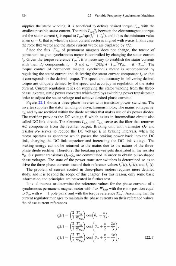
supplies the stator winding, it is beneficial to deliver desired torque Tem with the
smallest possible stator current. The ratio Tem/IS between the electromagnetic torque
and the stator current IS is equal to Tem/sqrt(id2 þ iq
2), and it has the minimum value
when id ¼ 0, that is, when the stator current vector is aligned with q-axis. In this case,the rotor flux vector and the stator current vector are displaced by p/2.
Since the flux CRm of permanent magnets does not change, the torque of
permanent magnet synchronous motor is controlled by changing the stator current
iq. Given the torque reference Tem*, it is necessary to establish the stator currents
with their dq components id ¼ 0 and iq ¼ (2/(3p)) ∙ Tem*/CRm ¼ K ∙ Tem*. Thetorque control of permanent magnet synchronous motor is accomplished by
regulating the stator current and delivering the stator current component iq so that
it corresponds to the desired torque. The speed and accuracy in delivering desired
torque are uniquely defined by the speed and accuracy in regulation of the stator
current. Current regulation relies on supplying the stator winding from the three-
phase inverter, static power converter which employs switching power transistors in
order to adjust the stator voltage and achieve desired phase currents.
Figure 22.1 shows a three-phase inverter with transistor power switches. The
inverter supplies the stator winding of a synchronous motor. The mains voltages uR,uS, and uT are rectified within the diode rectifier that makes use of six power diodes.
The rectifier provides the DC voltage E which exists in intermediate circuit also
called DC link circuit. The elements LDC and CDC serve as the filter that removes
AC components from the rectifier output. Braking unit with transistor QK and
resistor RK serves to reduce the DC voltage E in braking intervals, when the
motor operates as generator which passes the braking power back into the DC
link, charging the DC link capacitor and increasing the DC link voltage. The
braking energy cannot be returned to the mains due to the nature of the three-
phase diode rectifier. Therefore, the breaking power gets dissipated in the resistor
RK. Six power transistors Q1–Q6 are commutated in order to obtain pulse-shaped
phase voltages. The state of the power transistor switches is determined so as to
drive the three-phase currents toward their reference values ia*(t), ib
*(t), and ic*(t).
The problem of current control in three-phase motors requires more detailed
study, and it is beyond the scope of this chapter. For this reason, only some basic
information and principles are presented in further text.
It is of interest to determine the reference values for the phase currents of a
synchronous permanent magnet motor with flux CRm, with the rotor position equal
to ym, with p ¼ 1 pole pairs, and with the torque reference Tem*. Assuming that the
current regulator manages to maintain the phase currents on their reference values,
the phase current references
i�aðtÞ ¼2
3
T�em
CRm
� �cos ym þ p
2
� �;
i�bðtÞ ¼2
3
T�em
CRm
� �cos ym þ p
2� 2p
3
� �;
i�cðtÞ ¼2
3
T�em
CRm
� �cos ym þ p
2� 4p
3
� �; (22.1)
624 22 Variable Frequency Synchronous Machines
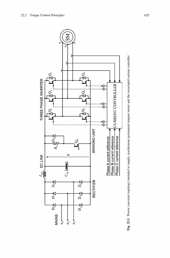
Fig.22.1
Power
convertertopologyintended
tosupply
synchronouspermanentmagnet
motorandtheassociated
currentcontroller
22.2 Torque Control Principles 625
result in the stator phase currents ia(t) ¼ ia*(t), ib(t) ¼ ib
*(t), and ic(t) ¼ ic*(t). They
produce the stator current vector with projections id ¼ 0 and iq ¼ (2/3) ∙ Tem*/CRm
on the axes of synchronous d–q coordinate frame. In turn, the motor delivers the
electromagnetic torque Tem ¼ Tem*.
22.3 Current Control Principles
Basic topology of static power converter intended to supply three-phase motor is
given in Fig. 22.1. By switching action of power transistors Q1–Q6, it is possible to
change the phase voltage supplied to the stator winding. The phase voltages ua, ub,and uc affect corresponding phase currents, thus providing the grounds for the
current control. The aim of the current control is obtaining the current components
id and iq that correspond to desired values. Current component id does not contributeto the torque, and it is mostly set to zero. Desired torque is obtained by establishing
current component iq in proportion to the desired torque. With rotor flux vector
collinear with d-axis, and with id ¼ 0, the vector of the stator current is orthogonal
to the flux. Further discussion outlines the basic principles of setting current
components id and iq to desired values.
The current components in d–q coordinate frame are uniquely defined by the
phase currents ia, ib, and ic. The problem of obtaining desired current components idand iq is therefore equivalent to the problem of controlling the phase currents. The
reference values of the phase currents ia*, ib
*, and ic* are calculated in (22.1), and
they depend on the torque reference Tem* and the rotor position ym. The torque
reference comes from the speed controller or the position controller, while the rotor
position is usually measured by the sensor attached to the rotor shaft. By setting the
phase currents according to (22.1), resulting vector of the stator current is perpen-
dicular to the vector of the rotor flux.
Within the current controller in Fig. 22.1, measured phase currents ia, ib, and icare compared to corresponding reference values in order to obtain the errors Dia,Dib, and Dic. Based upon these errors, the current controller generates gating signalsthat commutate transistor power switches. This changes the phase voltages in the
way which reduces the errors and eventually drives them toward zero. Ideally, the
current controller achieves the operation with ia(t) ¼ ia*(t), ib(t) ¼ ib
*(t), and
ic(t) ¼ ic*(t).
There are six switching power transistors in a three-phase inverter. The switches
are grouped in three phases, each one generating one of the phase voltages. The
inverter is supplied by DC voltage E, obtained from the DC link circuit. By turning
on the upper switch in one of the phases, the output phase is connected to the
positive plate of the DC link capacitor CDC. By turning on the lower switch, the
output phase is connected to the negative plate of the DC link capacitor CDC.
Assuming that the phase windings are star connected, and that the star point has
the potential in between the capacitor plates, turning on the upper or lower switch
results in the phase voltage ofþE/2 or�E/2. Hence, by turning on the upper switch
626 22 Variable Frequency Synchronous Machines
Q1 of phase a, the phase voltage ua(t) becomes þE/2, while turning on the lower
switch Q2 results in ua(t) ¼ �E/2.During one commutation period of T � 100 ms, the upper switch in phase a is
closed (on) during time interval tON, while in the remaining part of the commutation
period, T � tON, the upper switch is opened (off) while the lower switch is closed
(on). The phase voltage ua(t) is equal to +E/2 during time interval tON, and then it
remains �E/2 for the rest of the period (T � tON). The width tON of the positive
pulse can be varied continuously within the range 0 < tON < T. The average valueof the phase voltage during one period T is equal to ua(av) ¼ E ∙ (tON/T � 1/2).
Continuous change of the pulse width tON results in continuous change in the
average value of the phase voltage which ranges between �E/2 and þE/2. Varia-tion of the instantaneous value of the phase current ia(t) depends on the difference
between the instantaneous value of the phase voltage and the electromotive force
induced in the winding. Variation of the phase current during one commutation
period T depends on the average phase voltage ua(av) during one commutation
period. The change in the phase current is based on the voltage balance equation
ua ¼ RSia þ dCa/dt, where RSia is the voltage drop across the stator resistance
while dCa/dt is the electromotive force induced in one phase.
Distribution of magnetic field along the air gap depends on characteristics of
permanent magnet and the way of their mounting. The air-gap field is also affected
by the stator currents. The flux in the stator phase winding a isCa ¼ LSia þ CRm(a),
and it has two components. Component CRm(a) is produced by permanent magnets,
while the flux LSia depends on the stator currents.2 Component CRm(a) depends on
the amplitude and spatial orientation of the flux CRm, which is generated by
permanent magnets, which passes through the air gap, and which encircles the stator
windings. AmplitudeCRm is determined by characteristics of permanent magnets, by
the air gap d, and by properties of magnetic circuits. The spatial orientation of the
permanent magnet flux is determined by the rotor position ym. Therefore, the flux
CRm(a) depends on the amplitudeCRm and on the rotor position ym. With ym ¼ 0, the
rotor is aligned with magnetic axis of the phase a, resulting in CRm(a)¼CRm.
The changes in the stator flux Ca produce electromotive force dCa/dt. The laterhas two components, LS dia/dt and dCRm(a)/dt. The second component ea ¼ dCRm(a)/
dt is caused by the flux of permanent magnets, and it depends on the rotor speed
Om ¼ dym/dt.With constant rotor speed, the orientation of the permanent magnet flux is
determined by ym ¼ y0 þ pOmt. The part of this flux which encircles the phase
winding a is equal toCRmcos(ym). Besides, the phase winding has also the flux LSia;thus, the total flux of this phase is Ca ¼ Cmcos(ym) þ LSia. The voltage balance
equation becomes ua ¼ RSia þ LS dia/dt � omCmsin(ym). By neglecting the
2Notice at this point that the flux Ca in phase a depends on the phase current ia but also on the
phase currents ib and ic, due to a finite mutual inductance between the phase windings. Due to
ia ¼ �ib �ic and with reasonable assumption that Lab ¼ Lac, the flux component Laia þ Labib þLacic ¼ Laia þ Lab(ib þ ic) can be rewritten as LS ia.
22.3 Current Control Principles 627
voltage drop across the stator resistance and by adopting notation ea ¼ dCRm(a)/
dt ¼ �omCmsin(ym), the voltage balance equation becomes ua ¼ LS dia/dt þ еа.With that in mind, the rate of change of the stator current ia can be expressed as
diadt
¼ 1
LSua � eað Þ ¼ 1
LS�E� eað Þ: (22.2)
In operating conditions where E � jeaj, the phase voltage ua prevails in the
above expression. For ua ¼ +E/2, the rate of change of the stator current is positive,notwithstanding the electromotive force ea. For ua ¼ �E/2, the rate of change of
the stator current is negative. In other words, it is possible to obtain an increase of iaby turning on the switch Q1 and a decrease of ia by turning on the switch Q2. These
are the basic prerequisites for the current control. If the phase current ia does notcorrespond to the reference value, the current controller detects the error Dia ¼ ia
*
� ia. Then, it generates command signals for the inverter commutation so that the
error Dia is reduced and eventually removed. In cases where the error is positive
(Dia > 0), it is necessary to turn the upper switch Q1 on and to obtain dia/dt > 0.
This would reduce the error Dia ¼ ia* � ia. In cases where the error is negative
(Dia < 0), it is necessary to turn on the lower switch Q2 and to obtain reduction in
the phase current (dia/dt < 0). This would drive the error Dia ¼ ia* � ia toward
zero. A simple control law that proves efficient in controlling the stator currents of
three-phase AC motors is expressed by the following equation:
ua ¼ E
2� sign i�a � ia
� �; ub ¼ E
2� sign i�b � ib
� �; uc ¼ E
2� sign i�c � ic
� �:
With the above control law, transistor power switches Q1–Q6 are commutated
according to the sign of corresponding current error Di. Whenever the error
becomes positive, the upper switch is turned on, which increases the phase current
and reduces the error. As soon as the error becomes negative, the lower switch is
turned on to reduce the phase current and drive the error in positive direction.
Hence, the straight application of the above control law may result in elevated
commutation frequencies of the power transistors and increased commutation
losses. In order to contain the commutation frequency, it is possible to introduce
some hysteresis3 into comparators which determine the sign of the current error. In
this case, the commutation frequency is restrained by the hysteresis of comparators.
Practical current controllers operate in d–q coordinate frame. This means that the
errors Did ¼ id* � id ¼ 0 � id and Diq ¼ iq
* � iq are calculated from references
and feedback signals in d–q coordinate frame. The current controller calculates
the voltages ud and uq conceived to eliminate detected errors and drive the currents
3 Comparator with hysteresis H generates the output on the basis of the previous comparison and
on the new input. With previous output equal to +1, the input signal has to fall below �H in order
to produce the new output of �1. With previous output equal to �1, the input signal has to climb
above +H in order to produce the new output of +1.
628 22 Variable Frequency Synchronous Machines
id and iq to their references. The voltages ud and uq are transformed to the stationary
a–b coordinate system by inverse Park transform, and the obtained voltages ua andub are passed to the inverse Clarke transform to obtain the voltage references for the
phase voltages. Pulse-width-modulation-controlled three-phase inverter is used to
supply the desired voltages to the three-phase motor.
The algorithm which calculates the control variable udq ¼ ud þ juq from the
current error Didq ¼ Did þ jDiq is called control algorithm, while the regulator orcontroller is the device which implements the algorithm and provides the output.
Control algorithms are usually applied in digital form, by means of a program
which is executed by digital signal processor. Regulator can often be described by
its transfer function. The speed and quality of dynamic response depend on the
transfer function of the controller.
The power converter with six switching power transistors supplies the three-phase
stator winding by adjustable voltages. Therefore, it represents a controllable voltage
supply. By closing the feedback loop which controls the stator phase currents, an
appropriate current controller achieves that ia ¼ ia*, ib ¼ ib
*, and ic ¼ ic*. This
turns the current-controlled three-phase inverter into a current source. Hence, the
three-phase machine behaves as if it were supplied from a current source. The
operation of synchronous permanent magnet motor and controlled stator currents
is similar to the operation of DC machine with constant excitation with controller
armature current. The speed and accuracy in delivering the torque are fully
dependent on characteristics of the current controller.
22.4 Field Weakening
Current control can be accomplished in conditions where the electromotive force
e induced in the stator phase windings does not exceed the available phase voltage
E/2, where E is the DC voltage across the intermediate circuit called DC link circuit
of the three-phase inverter. Condition E/2 � jeaj ¼ jomCmsin(ym)j must be ful-
filled at every instant. In operation with id ¼ 0, the stator flux in d-axis of the
machine is equal to
Cd ¼ CRm þ Ldid ¼ CRm; (22.3)
while the stator flux in q-axis isCq ¼ Lqiq. In synchronous machines with surface-
mounted magnets, the stator inductances Ld and Lq are very low, and they range
from 0.01 to 0.05 relative units. Therefore, the flux along q-axis is considerablylower than the flux CRm. For this reason, it is justifiable to assume that the air-gap
flux amplitude equals Cm � CRm þ Lmid ¼ CRm ¼ Cn, where Cn is the rated
flux. At the rated rotor speed On ¼ on/p � E/CRm/p ¼ E/Cn/p, induced
electromotive force is equal to the rated voltage, which is at the same time the
maximum voltage available from the three-phase switching inverter. With id ¼ 0,
permanent magnet synchronous motor cannot exceed the rated speed.
22.4 Field Weakening 629
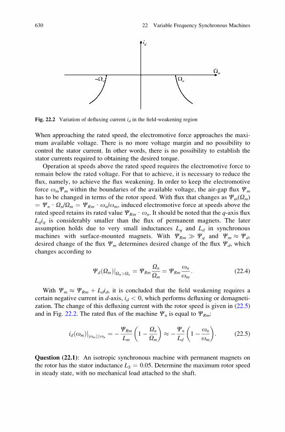
When approaching the rated speed, the electromotive force approaches the maxi-
mum available voltage. There is no more voltage margin and no possibility to
control the stator current. In other words, there is no possibility to establish the
stator currents required to obtaining the desired torque.
Operation at speeds above the rated speed requires the electromotive force to
remain below the rated voltage. For that to achieve, it is necessary to reduce the
flux, namely, to achieve the flux weakening. In order to keep the electromotive
force omCm within the boundaries of the available voltage, the air-gap flux Cm
has to be changed in terms of the rotor speed. With flux that changes as Cm(Om)
¼ Cn ∙ On/Om ¼ CRm ∙ on/om, induced electromotive force at speeds above the
rated speed retains its rated valueCRm ∙ on. It should be noted that the q-axis fluxLqiq is considerably smaller than the flux of permanent magnets. The later
assumption holds due to very small inductances Lq and Ld in synchronous
machines with surface-mounted magnets. With CRm � Cq and Cm � Cd,
desired change of the flux Cm determines desired change of the flux Cd, which
changes according to
CdðOmÞjOm>On¼ CRm
On
Om¼ CRm
on
om: (22.4)
With Cm � CRm þ Ldid, it is concluded that the field weakening requires a
certain negative current in d-axis, id < 0, which performs defluxing or demagneti-
zation. The change of this defluxing current with the rotor speed is given in (22.5)
and in Fig. 22.2. The rated flux of the machine Cn is equal to CRm:
id omð Þj omj j�on¼ �CRm
Lm1� On
Om
� �� �Cn
Ld1� on
om
� �: (22.5)
Question (22.1): An isotropic synchronous machine with permanent magnets on
the rotor has the stator inductance LS ¼ 0.05. Determine the maximum rotor speed
in steady state, with no mechanical load attached to the shaft.
Fig. 22.2 Variation of defluxing current id in the field-weakening region
630 22 Variable Frequency Synchronous Machines
Answer (22.1): In operation with high speeds that exceed the rated speed, it is
necessary to provide defluxing current in d-axis which has a negative value, id < 0.
This current reduces d-axis flux and maintains the electromotive force within the
limits of the available supply voltage. In the absence of the load torque, the electro-
magnetic torque and q-axis current are equal to zero. With iq ¼ 0, all of the available
stator current can be used for weakening the field in d-axis. At steady state, the currentin the stator windings must not exceed the rated current. Therefore, relative value of
the defluxing current that can be maintained permanently is id ¼ �1. By using the
expression for the defluxing current id(om) in the region of field weakening, one
obtains (1 � on/om) ¼ LS/CRm ¼ LS/Cn. Relative value of the rated flux is equal to
one, thus resulting in on/om ¼ 1 � 0.05 ¼ 0.95, which gives om ¼ 1.0526 on.
***
Previous example shows that synchronous motors with surface-mounted magnets
and with very low stator inductance cannot perform any significant increase of the
rotor speed above the rated value. Therefore, they cannot be used in the field-
weakening operation. On the other hand, induction servomotor can operate in field-
weakening mode and achieve the rotor speeds that exceed the rated speed by several
times. This is due to the fact that the flux in induction motors gets produced by the
stator current and not by permanent magnets. This shortcoming of synchronous
servomotors is the principal reason that induction servomotors are still in use. Namely,
other characteristics of these two types of servomotors go in favor of synchronous
motors. Induction machines have the power of losses significantly larger than syn-
chronousmachines.While the rotor losses in synchronousmachines are virtually zero,
there are considerable rotor losses PCu2 ¼ sPn in induction machines, proportional to
the slip. The absence of the rotor losses facilitates cooling of synchronous motors and
allows larger current and flux densities. Therefore, synchronous servomotors have
superior specific power and torque, and they are smaller than the equivalent induction
servomotors. Moreover, their rotors have much lower inertia J, which is beneficial inmost motion control applications. There are, however, applications of electrical
actuators where it is very important to provide the operation in the field-weakening
region and to provide the rotor speed that goes well beyond the rated speed. In these
applications, induction servomotors are advantageously used.
Synchronous motors with surface-mounted permanent magnets have a very low
stator inductance. This proves as an advantage in motion control applications such
as industrial robots and manipulators. With a low inductance LS, the rate of changeof the stator current dia/dt ¼ (ua � ea)/LS is very large and it reaches dia/dt � 104
In/s, which allows the electromagnetic torque Tem ¼ k jCRm iSj to make the
change from zero to the rated value in some 100 ms. Fast torque response
contributes to an increased bandwidth and improved closed loop performance in
speed control and position control applications. For this reason, synchronous
motors with surface-mounted magnets are applied in industry automation, robotics,
and many other motion control applications that employ speed and position control
loops. The absence of the field-weakening operations in these applications is not
considered a significant shortcoming.
22.4 Field Weakening 631
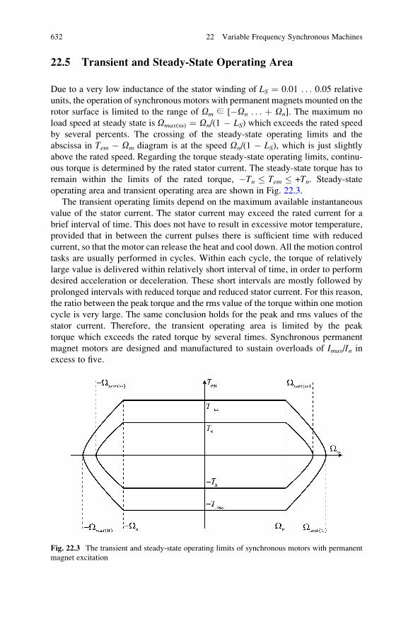
22.5 Transient and Steady-State Operating Area
Due to a very low inductance of the stator winding of LS ¼ 0.01 . . . 0.05 relative
units, the operation of synchronous motors with permanent magnets mounted on the
rotor surface is limited to the range of Om ∈ [�On . . . þ On]. The maximum no
load speed at steady state is Omax(ss) ¼ On/(1 � LS) which exceeds the rated speed
by several percents. The crossing of the steady-state operating limits and the
abscissa in Tem � Om diagram is at the speed On/(1 � LS), which is just slightly
above the rated speed. Regarding the torque steady-state operating limits, continu-
ous torque is determined by the rated stator current. The steady-state torque has to
remain within the limits of the rated torque, �Tn Tem +Tn. Steady-state
operating area and transient operating area are shown in Fig. 22.3.
The transient operating limits depend on the maximum available instantaneous
value of the stator current. The stator current may exceed the rated current for a
brief interval of time. This does not have to result in excessive motor temperature,
provided that in between the current pulses there is sufficient time with reduced
current, so that the motor can release the heat and cool down. All the motion control
tasks are usually performed in cycles. Within each cycle, the torque of relatively
large value is delivered within relatively short interval of time, in order to perform
desired acceleration or deceleration. These short intervals are mostly followed by
prolonged intervals with reduced torque and reduced stator current. For this reason,
the ratio between the peak torque and the rms value of the torque within one motion
cycle is very large. The same conclusion holds for the peak and rms values of the
stator current. Therefore, the transient operating area is limited by the peak
torque which exceeds the rated torque by several times. Synchronous permanent
magnet motors are designed and manufactured to sustain overloads of Imax/In in
excess to five.
Fig. 22.3 The transient and steady-state operating limits of synchronous motors with permanent
magnet excitation
632 22 Variable Frequency Synchronous Machines
The peak current capability is limited by the motor construction but also by the
characteristics of the three-phase inverter which supplies the stator windings.
Semiconductor power switches within the inverter comprise tiny silicon crystals
with very low thermal capacity and with limited density of electrical current. In
cases where the current density within semiconductor exceeds certain limit, there is
an abrupt increase in temperature which changes the structure of the crystal and
causes permanent damage to the semiconductor power switch. Semiconductor
power switches can withstand electrical currents that exceed declared limits but
only for relatively short intervals of time, measured in milliseconds. Large peak
currents can also damage the synchronous servomotor. Large stator current may
damage the permanent magnets. The stator currents produce the stator
magnetomotive force, which depends on the current amplitude and on the number
of turns. With large currents, the stator magnetomotive force produces large
demagnetization field within the magnets. In B-H characteristic of permanent
magnets, the operating point (B,H) of the magnets is moved closer to coercive
field HC < 0, where the induction B of permanent magnets reduces to zero. For
most permanent magnet materials, reaching the coercive field HC damages the
magnet. Having reached this operating point, their remanent induction cannot
return to the initial value. Instead, the remanent induction is decreased by two or
three times. Therefore, the maximum permissible stator current is set to the value
that does not bring the risk of damaging the magnets. At the same time, it has to be
compatible with peak current capability of semiconductor power switches that are
used within the three-phase inverter attached to the stator windings.
The maximum torque Tmax which defines the limits of the transient operating
area is determined by the peak current Imax. The maximum no load speed Omax(tr)
that can be reached over short time intervals is determined by expression Omax(tr)
¼ On/(1 � ImaxLS), where the stator inductance and the peak current are both
expressed in relative units.
Question (22.2): An isotropic machine with permanent magnets on the rotor has
stator self-inductance of LS ¼ 0.05. Find the maximum rotor speed that can be
reached for a short interval of time. The peak current capability is Imax ¼ 5, while
the mechanical load attached to the shaft is equal to zero.
Answer (22.2): By using expression for demagnetizing current id(om) in the field-
weakening region, one obtains that (1 � on/om) ¼ ImaxLS/CRm ¼ ImaxLS/Cn. Rel-
ative value of the rated flux is equal to one; thus, the ratio of the rated speed and the
maximum speed is determined by on/om ¼ 1 � 5 ∙ 0.05 ¼ 0.75, resulting in
Om ¼ 1.33 ∙ On.
***
Synchronous permanent magnet machines are also used in applications that
require high efficiency, low losses, and high specific power, but where it is not
necessary to effectuate quick changes of the electromagnetic torque. These
applications do not include motion control tasks, and they do not use synchronous
machines in speed control and position control loops. Some of the examples are the
22.5 Transient and Steady-State Operating Area 633
motors used in blowers, household appliances, and HVAC systems but also the
generators in renewable sources of electrical energy, such as the wind turbines, the
motors in electrical vehicle propulsion, auxiliary drives in automotive field, and
similar. Superior efficiency, lower weight, and lower inertia of synchronous per-
manent magnet motors are the reasons for their use instead of corresponding
induction machines. In order to improve the field-weakening performance of
synchronous permanent magnet machines, it is possible to remove the permanent
magnets from the rotor surface and to burry them deep into the rotor magnetic
circuit. This results in larger values of the stator self-inductance. According to
(22.5), larger LS improves capability of synchronous machines to operate above
the rated speed. Yet, the field-weakening performance of synchronous permanent
magnet machine is inferior to that of induction machines. Synchronous
permanent magnet machines that operate in the field-weakening range require
considerable demagnetization current id < 0 which does not contribute to the
torque, while increasing the amplitude of the stator current IS ¼ sqrt(id2 þ iq
2)
and increasing the copper losses. For that reason, the applications requiring
prolonged operation in field-weakening mode with considerable ratio Om/On call
for an induction machine.
634 22 Variable Frequency Synchronous Machines
Bibliography
1. Kloeffler RC, Kerchner RM, Brenneman JL (1949) Direct current machinery. McMillan,
New York
2. Kimbark EW (1956) Power system stability. Synchronous machines, vol III. Wiley, New York
3. White DC, Woodson HH (1959) Electromechanical energy conversion. Wiley, New York
4. Shortley GH, Williams DE (1961) Elements of physics. Prentice-Hall, Englewood Cliffs
5. Edwards JD (1973) Electrical machines: introduction to principles and characteristics.
Intertext Books International Textbook Company Limited, Aylesbury
6. Slemon GR, Straughen A (1980) Electrical machines. Addison Wesley, Reading
7. Petrovic M (1987) Ispitivanje elektricnih masina. Naucna knjiga, Beograd
8. Vukosavic SN (2007) Digital control of electrical drives. Springer, New York
9. Wildi T (2006) Electrical machines, drives and power systems. Pearson Prentice Hall, Upper
Saddle River
10. Seeley S (1958) Electromechanical energy conversion. McGraw-Hill, New York
11. Brown D, Hamilton EP (1984) Electromechanical energy conversion. McMillan, New York
12. Fitzgerald AE, Kingsley C (1961) Electrical machinery. McGraw-Hill, New York
13. Alger PL (1965) Induction machines. Gordon and Breach, New York
14. Chalmers BJ (1988) Electric motor handbook. Butterworth, London
15. Krause PC, Wasynczuk O, Sudhoff S (1995) Analysis of electric machinery. IEEE Press,
Piscataway
S.N. Vukosavic, Electrical Machines, Power Electronics and Power Systems,
DOI 10.1007/978-1-4614-0400-2, # Springer Science+Business Media New York 2013
635
Index
A
AC. See Alternating current (AC)
Acceleration, 12, 21, 122, 305, 318, 322, 462,
514, 515, 579, 621, 623, 632
AC machines. See Alternating current (AC)
machines
Active power, 445, 571, 576, 577, 580, 581,
586, 587, 590
Actuator, 413, 621, 631
Air gap, 18, 48, 59, 81, 109, 131, 153–183, 224,
271, 302, 367, 379, 428, 478, 523, 545,
571, 596, 622
Air gap field, 84, 173, 185, 251, 627
Air gap flux, 376, 428, 433, 435, 452, 503, 510,
526, 568, 571, 630
Air gap power, 379, 429–431, 438–441, 446,
468, 470, 471, 473, 478, 481, 492,
545, 622
Alternating current (AC), 1–3, 7, 9, 19, 20, 71,
96, 102, 104, 129, 134, 135, 139, 142,
145–152, 186, 187, 191, 193, 194, 206,
209, 210, 213, 215, 224, 229, 235, 243,
260, 265, 266, 269, 270, 273, 277, 292,
322, 325, 326, 333–335, 338, 340, 341,
345, 369, 371, 373, 376, 380, 382, 386,
414, 419, 432, 469, 476, 477, 481, 482,
494, 498, 499, 501, 521, 522, 524, 535,
536, 555, 572, 576, 585, 586, 591, 607,
610, 616, 624, 628
Alternating current (AC) machines, 18, 19, 88,
121, 141–142, 145, 149, 151, 213, 230,
260, 265, 345, 355, 363, 371, 387, 449,
483, 521, 603
Ampere law, 20, 49, 60–62, 66, 69
Anisotropic machines, 562, 565, 566, 571, 577,
578, 581–584, 633
Anisotropic rotor, 565–567
Apparent power, 431, 443, 445, 577, 580, 581
Armature current, 286, 287, 291, 293–295,
298–300, 303, 308–312, 315–317, 319,
321, 323, 325, 327, 328, 330, 333–339,
345, 346, 348–351, 353, 355, 357,
358, 629
Armature reaction, 281, 283, 286–290, 303
Armature voltage, 308–312, 315–319,
322–326, 330–336, 338, 352, 449
Armature winding, 287, 290–295, 298–300,
302–305, 307–313, 316, 319–323, 325,
326, 329, 330, 332, 334–336, 338,
340, 341, 349, 352, 358–360, 363,
449, 503
Asynchronous machines, 6, 23, 88, 210,
521, 522
Auxiliary poles, 284–291, 303, 358
Auxiliary power supplies, 340
Average torque, 133, 139
Average voltage, 102, 331–333, 339, 496–498,
621, 622
Axial component of magnetic field, 159, 161
Axial component of the rotor field, 177
B
Back electromotive force, 55–57, 61
Balance of power, 90, 120, 122, 124–125, 430,
472–473, 563
Balance of power of induction machine, 537
Base impedance, 443, 444
Base speed, 445
Base torque, 446
Base value, 442–449
Basic frequency component, 242, 333
Belt distribution factor, 232
Belt factor, 223, 232, 236–238, 240, 241, 486
S.N. Vukosavic, Electrical Machines, Power Electronics and Power Systems,
DOI 10.1007/978-1-4614-0400-2, # Springer Science+Business Media New York 2013
637
Bipolar junction transistors (BJT), 326–330,
477
Block diagram, 6, 125, 306–309
Block transformer, 9, 605
Blondel transform, 423
Blower, 317, 318, 634
Bobbin, 33
Braking device, 341
Braking energy, 341, 624
Braking unit, 624
Breakdown frequency, 463
Breakdown slip, 427, 463–465, 478, 479,
492, 502
Breakdown torque, 427, 463–467, 479, 492,
502, 506, 511–514, 518
Breakdown voltage, 344
Brushes, 210, 264–266, 268–276, 278–284,
286–288, 291–294, 297, 303, 310, 311,
316, 319, 321, 327, 333, 369, 370, 479,
480, 482, 522, 533, 534
Buried magnets, 522, 537, 541–544, 621
C
Cage rotor, 368–370, 373, 400–403, 405, 408,
409, 418, 419, 427, 430, 431, 433–436,
452, 456, 469, 515, 516, 529, 530, 604
Cartesian coordinate system, 13, 26, 387
Cascades, 482
Characteristic of magnetization, 63, 64, 95, 105
Characteristic polynomial, 597, 598, 602, 603
Chord factor, 223, 232–237, 486
Circular arcing, 280
Clarke transform, 19, 387–389, 391–398,
400, 428, 429, 432, 439, 448, 550–553,
574, 629
Coefficient of Clarke transform, 424, 438
Coefficient of efficiency, 90, 91, 100, 103, 427,
431, 446, 472, 473, 515
Coefficient of electromagnetic torque, 298
Coefficient of electromotive force, 298
Coefficient of inductive coupling, 71
Coil, 18, 32, 33, 56, 57, 59, 86, 87, 89, 94, 95,
101, 104, 109, 113, 231, 303, 368, 370,
372, 373, 401, 538, 580, 590, 607
Cold rolled sheets, 531
Collector, 210, 264–268, 270, 272, 274, 276,
280, 284, 303, 316, 329, 340, 369
Collector segments, 264, 266–268, 272, 274,
275, 278–280, 283, 286, 292, 294
Commutation, 260, 270–273, 278–284, 286,
289, 292, 326, 327, 490, 622, 628
Commutation frequency, 328, 338, 496–499,
543, 628
Commutation losses, 326, 327, 331
Commutation period, 496, 622, 627
Commutator, 151, 210, 260, 261, 263, 266,
269, 272–273, 282, 284, 303
Commutator segments, 264, 282
Compensation winding, 285, 286, 288–291, 358
Complex notation, 13, 420, 421, 425, 558,
573, 576
Compound winding, 241–242
Concentrated winding, 88, 154, 173–175, 200,
203, 214, 216, 230, 240, 255, 256, 436
Conduction losses, 326
Conductor line density, 201, 205
Constant flux region, 353, 356, 357, 476, 509
Constant power region, 509
Constant torque region, 509
Construction of induction machines, 365,
513–519
Contactless excitation system, 535
Control algorithm, 309, 411, 413, 414, 571, 629
Controller, 14–16, 308, 309, 413, 491, 506,
586, 610, 625, 628, 629
Control variables, 307–309, 413, 629
Convention of representing magnetic field by
vector, 182–183
Conversion cycle, 46–48, 94, 96
Conversion losses, 6, 17–19, 53, 54, 89–91, 99,
343, 346, 353, 450, 493
Conversion power, 3, 116, 118, 139, 177,
209, 555
Coordinate transform, 379, 387, 390, 391, 398,
415, 439, 545, 551, 552
Copper losses, 91, 212, 306, 358, 359, 429,
430, 443, 446, 450, 451, 463, 469, 470,
472, 514, 529, 537, 538, 563, 564, 568,
582, 598, 634
Copper losses in stator windings, 469, 581
Core flux, 59, 61, 66, 67, 70
Counter electromotive force, 55, 57, 77, 107,
223, 225, 226, 228, 254, 456
Coupling, 2, 25, 41–57, 65, 81, 99, 133, 177,
188, 300, 357, 400, 442, 535, 563,
590, 596
Coupling field, 25, 33, 36, 39, 41–57, 94–97,
99, 112–116, 124, 564
Critical speed, 510–513
Cross saturation, 300, 408
CRPWM. See Current regulated pulse width
modulated inverters (CRPWM)
Curie temperature, 246
638 Index
Current regulated pulse width modulated
inverters (CRPWM), 529
Current regulator, 529, 624
Current ripple, 335–339, 499–502, 518, 536,
543
Cylindrical machine, 18, 81, 83, 119, 153,
155, 161, 162, 168, 177, 181, 188,
201, 530
D
Damped LC circuit, 600–602
Damped oscillations, 600, 601
Damper winding, 545, 595, 603–607, 609, 611,
613–615, 617–619
Darlington, 329
DC bus, 494, 495, 497, 501
DC generator, 9, 36, 259, 260, 299, 319–321,
323, 610
DC link, 340, 341, 494, 496, 499, 624, 626
DC link circuit, 341, 494, 495, 624, 626, 629
DC machine power supply, 321–342
DC machines. See Direct current (DC)machines
DCmachine with permanent magnets, 262, 306
Declared values, 362, 363
Deep slot, 518
Defluxing, 630, 631
Delta connection, 371, 383, 524
Demagnetization, 633, 634
Demagnetizing current, 633
Density of the field energy, 44, 48, 188
Diametrically positioned conductors, 155, 230,
232, 237, 400, 484
Dielectric materials, 33–35, 37, 42, 44, 45,
47, 344
Dielectric strength, 47, 48, 102, 344
Differential equation describing changes of
angular speed, 301
Differential equations of voltage equilibrium,
381
Differential permeability of permanent
magnets, 542, 566
Differentiation operator, 307
Diode rectifier, 2, 326, 327, 331, 340, 477, 481,
482, 494, 535, 536, 624
Direct axis, 288, 289, 299, 306, 566, 573
Direct current (DC) machines, 9, 88, 121, 129,
209, 259–364, 369, 449, 483, 629
Distributed winding, 18, 173–175, 186, 191,
201–203, 205, 206, 223, 224, 230–232,
236, 242, 244–251, 498
Distribution networks, 3, 340, 580, 581, 605
Double cage (rotor), 515, 516
Double cage induction machines, 515, 516
Double fed machines, 129, 130, 135, 138,
139, 141
Double side supplied converters, 129
Driving torque, 5, 11, 124, 273, 317, 321, 322,
586, 592, 600
Driving turbine, 117, 120, 321, 546, 586, 587
Dynamic braking device, 341
Dynamic electromotive force, 223, 224, 242
Dynamic model, 16, 99, 100, 260, 305, 380,
381, 390, 427, 546
E
Eddy currents, 59, 71–79, 89, 105, 121,
285, 360–362, 367, 430, 469, 488,
531, 604
Electrical access, 4, 5, 83, 87, 99, 114, 124,
379, 533
Electrical and mechanical time constants, 596
Electrical energy, 1–10, 21, 22, 25, 27, 30,
31, 36, 43, 44, 51–55, 82, 83, 90, 97,
116, 117, 259, 294, 319, 321, 322,
325, 326, 340, 341, 370, 468, 472,
473, 475, 546, 563, 574, 586, 588,
592, 605, 634
Electrical generator, 1–3, 5–7, 18, 67, 83, 605
Electrical insulation, 75, 76, 78, 89, 344, 346,
362, 367, 369, 451, 504, 533
Electrical motors, 1–3, 5, 9, 10, 12, 16, 18,
20–22, 91, 124, 308, 321, 322, 330, 331,
357, 413, 580, 622
Electrical subsystem, 100, 108, 117, 124, 423,
425, 546, 593, 595, 596
Electrical subsystem of induction machines,
380, 400, 403, 404, 424
Electrical subsystem of isotropic machines,
561–562
Electrical vehicle propulsion, 634
Electromagnet, 59, 522
Electromagnetic excitation, 261, 532, 533, 565
Electromagnetic force, 2, 3, 7, 25, 26, 28,
30–32, 39, 51–54, 81, 82, 119, 143, 263,
287, 288, 470, 527, 564, 583
Electromagnetic torque, 6, 55, 81, 99, 133, 153,
185, 243, 261, 300, 344, 366, 381, 428,
478, 521, 545, 571, 595, 623
Electromagnetic torque at high slip, 462
Electromagnetic torque at low slip, 461
Electromechanical conversion, 3, 4, 18, 22, 25,
33, 38, 39, 41, 46, 47, 49, 50, 52, 53, 59,
60, 83, 90, 94, 99, 103, 112, 114–117,
Index 639
125, 127, 133, 177, 185, 211, 310, 317,
324, 325, 359, 361, 407, 469, 487, 522,
563, 564, 575, 583, 586
Electromotive force, 2, 27, 52, 61, 88, 99, 154,
223, 261, 304, 351, 366, 385, 433, 489,
521, 546, 573, 605, 627
Electromotive force in a winding, 230–241
Electromotive force in distributed winding,
244–251
Electromotive force in one turn, 224–230, 233,
236, 241, 255, 389
Electromotive force of compound winding,
241–242
Electromotive force of self induction, 224
Electromotive forces induced in the windings,
70, 107
Electromotive force waveform, 175, 228–229,
250
Electrostatic field, 29, 33, 35, 41–50
Electrostatic machine, 18, 33, 41, 44, 48, 50
End effects, 161
Energy efficiency, 21, 22, 331, 369, 451, 622
Energy of electrical field, 35, 301, 381, 424
Energy of magnetic field, 68, 69, 118, 138, 191,
301, 549
Energy of the coupling field, 36, 48, 95–97, 99,
112–115, 124
Equations of mathematical model, 126–127
Equivalent circuit, 15–17, 19, 260, 261, 299,
301, 304, 309, 312, 319, 336, 387, 411,
412, 427, 432, 434–439, 445, 447–458,
462, 465, 471–473, 480, 502, 503, 546,
573–576, 578, 588, 612
Equivalent leakage inductance, 453, 454,
464, 617
Equivalent magnetic pressure, 519
Equivalent pressure, 35, 519
Equivalent two phase machine, 385, 388, 390,
395, 396, 411, 548, 552
Excitation flux, 88, 261, 262, 285–288, 290,
291, 294–306, 308, 310, 311, 318, 321,
323, 351–353, 355, 357, 358, 360, 503,
532, 533, 546, 555, 564, 565, 568, 572,
573, 577, 580, 583, 591, 610, 612, 614
Excitation winding, 7, 59, 88, 261, 299, 344,
503, 521, 546, 591, 595, 622
Expression for electromagnetic torque, 126,
211, 301, 441
Expression for the torque, 21, 207, 208, 212,
381, 425, 442, 546
External field, 51, 54, 57, 63, 64, 262, 538–540
External resistor, 294, 370, 479–481
F
Faraday law, 3, 20, 50
Feromagnetic, 2, 25, 48, 59, 81, 104, 131,
154, 200, 296, 300, 346, 381, 450,
487, 531, 546
Ferrite, 76, 488, 538
Field energy, 35–37, 41–45, 47, 48, 81, 93–97,
113, 114, 118, 133, 138, 185, 188, 189,
191, 194, 422, 428, 431, 549
Field weakening, 19, 261, 343, 352–357, 476,
504–511, 532, 537, 544, 568, 621,
629–631, 634
Field weakening region, 353, 357, 506,
508–510, 544, 630
Finite zeros, 597
Flux base value, 444
Flux conservation law, 61–62, 69, 485, 541
Flux density, 25–29, 32, 38, 74, 213,
450, 490
Flux in one rotor turn, 198–200
Flux in one stator turn, 196–198, 526
Flux in one turn, 110, 175, 182, 194–198,
200–203, 205, 214–217, 225–226,
246–248, 297, 374, 405, 435, 526
Flux in single turn, 132, 194
Flux linkage, 3, 20, 185, 223, 300, 301, 379,
390, 399, 404, 409, 415, 417, 419, 420,
425, 427, 433, 436, 438, 445, 448, 449,
526, 545, 546, 549, 553, 555, 557, 559,
561, 562, 566, 574, 576, 593, 595, 596,
608, 610, 615, 616
Flux of permanent magnets, 572, 581, 623,
627, 630
Flux per turn, 18, 61, 145, 552
Flux vector, 18, 28, 63, 108, 143, 170,
185, 262, 372, 383, 444, 522, 549,
575, 624
Force, 2, 25, 41, 59, 81, 99, 132, 153, 187, 223,
261, 301, 351, 366, 380, 433, 484, 521,
546, 573, 600, 623
Four pole machines, 141, 142, 490, 492, 529
Four quadrant operation, 318
Four quadrant power converter, 325–330
Fractional pitch coil, 231
Fractional pitch turn, 231, 233–236, 241,
244, 278
Free wheeling diodes, 329–330
Friction torque, 120, 123, 305, 308, 311, 470
Full pitch coil, 231
Fundamental frequency component, 498
Fundamental harmonic, 233, 236, 241, 246,
249, 251, 253
640 Index
G
Generalized Ampere law, 49, 66
Generator mode, 6, 30–31, 53, 55, 83, 90,
116, 117, 123, 124, 311, 317, 319,
321, 323–325, 341, 409, 427, 463, 465,
466, 468, 472, 473, 479, 587, 592, 600
Good model, 17, 100, 101, 103
Grooves, 86, 153, 229, 230, 237
H
Halted rotating field, 147
Harmonics suppression, 238–241
Harmonics suppression of winding belt,
238–241
Heaviside function, 597
High speed operation, 353–354, 356
High voltage transmission network, 585, 605
Homogeneous field, 102
Hopkins law, 67
Hot rolled sheets, 531
Household appliance, 634
Hunting of synchronous machines, 596–600
HVAC systems, 634
Hydro-electric power plants, 534
Hyperbola of constant power, 356, 357
Hysteresis curve, 71, 72
Hysteresis losses, 59, 71–72, 75, 89, 488, 531
I
Ideal switch, 326
IGBT. See Insulated gate bipolar transistors
(IGBT)
Impedance invariance, 392
Impedance invariant transform, 551
Inadequate commutation, 280
Inductance invariance, 392, 411
Inductance matrix, 109, 114–118, 126, 127,
132, 137, 138, 301, 379, 381, 383, 400,
404, 407–410, 418, 419, 421–425, 546,
553–554, 556–558, 561, 615
Inductance matrix in dq frame, 421–423,
556–558
Inductance matrix of induction machines, 404,
407–410, 418, 424, 425
Inductance matrix of synchronous machines,
546, 554, 561, 614
Induct current, 287
Induction machines, 129, 130, 142, 147, 148,
151, 152, 365–377, 380–425, 427–473,
475–519, 521, 522, 526, 529, 530, 537,
538, 554, 583, 604, 622, 631, 634
Inductor induct, 287
Industrial robots, 9, 16, 21, 331, 413, 476, 546,
586, 621, 631
Inertial torque, 305, 314, 602
Insulated gate bipolar transistors (IGBT),
326–330, 340, 477
Insulation lifetime, 344
Interaction of the stator and rotor fields,
185–188, 529, 563
Intermediate circuit, 624, 629
Intermediate DC circuit, 340, 341, 494
Intermittent load, 349
Intermittent mode, 349
Internal mechanical power, 90, 91, 470–473, 564
Invariance, 391–398, 411
Inverter, 1, 2, 265, 476, 477, 482, 483, 488, 492,
500, 501, 506, 529, 624, 626, 628, 633
Inverter arms, 494
Inverter supplied synchronous machines,
621–622
Iron core, 60, 66, 88, 119, 132
Iron losses, 59, 75–76, 91, 100, 103–105, 121,
124, 126, 155, 285, 350, 353, 355,
358–362, 367, 381, 410, 424, 429, 430,
438, 446, 450, 469, 470, 472, 488, 531,
536, 537, 546, 563
Iron losses in rotor magnetic circuit, 431,
469, 470
Iron losses in stator magnetic circuit, 431,
469, 582
Isotropic rotor, 136, 561, 562
Isotropic synchronous machine, 563, 572, 576,
578, 590, 630
J
Joule effect, 52, 55, 116, 124, 317, 331, 345,
349, 359
Joule losses, 52, 78, 345, 351, 358, 431, 479
K
Kinetic energy, 120–122, 125, 341, 362, 588
Kirchhoff law, 3, 20
Kloss formula, 465–466
L
Laminated ferromagnetics, 76–79
Lamination, 75, 79, 89, 103, 285, 531
Laplace operator, 307, 597, 602
Laplace transform, 20, 306, 307, 334, 412, 500,
597, 601
Index 641
Lap winding, 278
Leakage flux, 61, 70, 71, 86, 109–112, 177,
404–407, 452, 454–456, 493, 499, 514,
516–518, 528, 533, 564
Leakage flux in rotor winding, 112, 405
Leakage flux in stator winding, 112, 499
Leakage inductance, 18, 111, 112, 393, 394,
404–407, 409, 433, 434, 447, 451–456,
458, 463, 464, 486, 499, 501, 510, 514,
516–518, 611, 614, 616, 617
Leakage inductance of stator windings, 434,
611
Linear commutation, 286
Linear converter, 50–53
Linear electrical machines, 10
Linear motors, 4
Line density of conductors, 155, 157, 173, 201,
250, 251, 526
Line frequency, 10, 21, 22, 38, 75, 142, 326,
340, 369, 370, 386, 430, 431, 435, 436,
455, 462, 481, 482, 487, 513, 515, 516,
585–590, 592
Load characteristics, 313, 314, 317,
319, 480
Load torque, 5, 11, 12, 19, 300, 305, 310–314,
317, 321, 349, 451, 462, 463, 466–468,
480, 579, 592, 593, 597–600, 603,
623, 631
Locked rotor test, 455
Lorentz law, 3, 20, 25
Losses due to rotation, 99, 125, 358, 361, 427,
469–472
Losses in armature winding, 359
Losses in excitation winding, 351, 359
Losses in magnetic circuit, 71–79, 89, 103,
121, 301, 358, 450, 469, 531
Losses in mechanical subsystem, 120–121, 469
Losses in rotor cage winding, 469
Losses in the coupling field, 99, 115
Loss power density, 71
Low-pass nature of electrical machines,
334–335
Lumped parameter, 101, 104
Lumped parameter networks, 103, 104, 301
M
Magnetic circuits, 2, 28, 48, 59–79, 81, 99, 129,
153, 185, 224, 261, 300, 343, 365, 389,
427, 483, 521, 552, 582, 596, 622
Magnetic coupling field, 3, 4, 18, 39, 41–57,
81, 93, 94, 100, 103–106, 113, 116, 117,
124, 126, 133, 136, 137, 188, 563
Magnetic dipoles, 64, 71, 72, 538–540
Magnetic field, 2, 25, 41, 59, 81, 104, 129,
153–183, 185, 224, 273, 301, 359,
365, 405, 428, 475, 521, 549, 572,
605, 627
Magnetic forces, 13, 30
Magnetic permeability, 62, 188, 452
Magnetic poles, 23, 51, 85, 141, 170, 187, 232,
262, 361, 411, 440, 475, 524, 553
Magnetic poles of induction machines, 148,
371, 483
Magnetic resistance, 18, 20, 28, 31–33, 59,
65–69, 78, 79, 84, 87, 109, 111, 119,
131, 132, 136, 149, 150, 172, 177, 204,
214, 215, 217, 281, 283, 285, 286, 297,
300, 302, 303, 306, 334, 373, 404, 406,
407, 409, 435, 452, 454, 455, 487, 514,
522, 526, 531, 533, 537, 540, 541, 543,
544, 561, 562, 564–567, 583, 616, 623
Magnetic saturation, 95–97, 126, 211–213,
300, 381, 404, 408, 410, 424, 454
Magnetic voltage, 20, 67
Magnetic voltage drop, 215, 285
Magnetizing branch, 436
Magnetizing branch voltage, 448, 462, 503
Magnetizing characteristic of permanent
magnet, 538
Magnetizing current, 433, 435, 438, 439,
447, 448, 451, 453, 456, 457, 465,
503, 504, 509
Magnetizing flux, 433, 447, 448, 456
Magnetizing inductance, 451–452, 457, 458
Magnetomotive force, 3, 65, 81, 113, 132, 153,
190, 242, 261, 301, 372, 380, 435, 484,
521, 547–548, 633
Magnetostriction, 38–39
Mains supplied machines, 436, 476–477, 483,
487, 506, 513–517
Making the rotor windings, 269, 274–278, 532
Mathematical model, 14–19, 99, 100, 126–127,
261, 299, 300, 305–306, 309, 365, 379,
381, 383, 388, 391–393, 398, 410–411,
413, 414, 419, 423, 424, 431, 438, 452,
455, 521, 545–569, 571, 607, 619
Mathematical model in stationary coordinate
frame, 19
Maxwell equation, 49, 50, 104, 166
Mechanical characteristic, 15–17, 19, 99, 100,
260, 261, 291, 299, 311–319, 343–345,
380, 427, 457–464, 466, 476–480, 502,
503, 506, 507, 584–585
Mechanical characteristic of induction
machine, 427, 463
642 Index
Mechanical characteristic of synchronous
machine, 546
Mechanical commutator, 260, 263–266, 269,
272–274, 277, 292, 293, 303, 357,
369, 483
Mechanical interaction, 7, 11, 93, 153, 187, 191
Mechanical losses, 89, 90, 116, 121, 360, 430,
451, 469–470, 537
Mechanical losses due to rotation, 99, 358,
427, 469
Mechanical power, 6, 7, 10, 18, 21, 26–28, 31,
32, 49, 50, 52–54, 83, 90, 91, 99, 116,
117, 120, 122, 124, 319, 321, 322, 356,
359, 361–362, 427, 429–431, 471–473,
478, 481, 564, 568, 583, 585, 588,
589, 591
Mechanical subsystem, 18, 81, 89, 94, 100,
116, 119–126, 304, 360, 380, 381, 430,
469–471, 473, 545, 546, 557, 564, 592,
593, 595, 596, 599, 622
Mechanical work, 1–7, 10, 25–28, 30, 31, 33,
35, 36, 38, 41, 43–45, 47, 48, 50–52, 55,
94, 96, 112, 116–118, 123, 218, 259,
319, 321, 322, 341, 473, 475, 546, 563,
586, 592
Metal oxide field effect transistors (MOSFET),
326–330, 477
Microscopic Ampere current, 63
Model of mechanical subsystem, 122–124
Modulation index, 337, 338
Moment of inertia, 12, 121
MOSFET. See Metal oxide field effect
transistors (MOSFET)
Motion control, 16, 38, 308, 331, 369, 475,
476, 529, 544, 546, 585, 586, 621–623,
631–633
Motion cycle, 318, 322, 323, 325
Motion resistance losses, 121, 124
Motor mode, 6, 82, 83, 90, 116, 117, 123, 317,
323–325, 465, 466
Multiple pole pairs, 361, 440, 460, 475, 488,
547, 557
Multipole machines, 141, 440, 486–490,
492, 572
Mutual flux, 109–111, 136, 374, 375, 404–407,
435, 436, 452, 472, 499, 503, 526, 533,
535, 610, 616
Mutual inductance, 18, 108–119, 126, 127,
129, 130, 135, 137–138, 141, 202, 299,
300, 373, 383, 393, 394, 399, 404,
406–408, 418, 421–423, 442, 454,
548, 549, 554, 556, 557, 562, 610,
611, 615–618
N
Nameplate data, 363–364
Name plate values, 19
Natural characteristic, 345, 584
Neglected phenomena, 99, 103–106
Neutral zone, 272, 280–286, 288–290, 292,
297, 303
Newton differential equation, 16, 127, 381, 545
Newton differential equation of motion, 126,
379, 380, 546, 595
Newton equation, 12, 123, 126, 301, 311, 314,
381, 410, 429, 466, 546, 593, 600
Newton equation of motion, 429, 466, 546,
561, 586, 588, 623
Newton law, 83
No load conditions, 291, 294, 349, 433, 593
No load speed, 311, 312, 315–317, 502, 633
No load test, 451
Nonlinearity of magnetic circuit, 300, 301
Non-stationary matrix, 126, 554
Normalized value, 442
North magnetic pole, 141, 142, 170, 172, 176,
182, 187, 232, 262, 263, 266, 268–270,
275–277, 281, 282, 285, 292, 293, 373,
485–487, 490, 529
North pole, 142, 169, 173, 183, 263–265, 269,
273, 276, 285, 287, 293, 294, 297, 411,
484, 487
Number of poles, 141, 142, 440, 441, 475–477,
483, 486–493, 522, 530, 547,
579, 591
O
Operation of commutator, 272–273
Oscillatory responses, 598
Overload operation, 343
P
Parasitic capacitances, 103–105, 301, 381,
424, 546
Parasitic effects, 17, 101, 130
Park coordinate transform, 379, 439, 545
Park rotational transform, 417, 422, 558,
560, 576
Park transform, 390, 415–416, 418, 420, 421,
423–425, 428, 431, 432, 434, 554–557,
559–561, 571, 574, 629
Peak current capability, 633
Peak power capability, 598
Peak torque capability, 14, 544
Periodic electrical currents, 264
Index 643
Permanent magnet(s), 22, 27, 51, 59, 61, 63,
81, 84, 88, 93, 119, 121, 129, 130, 148,
152, 185, 195, 210, 224–229, 235, 242,
243, 245–246, 251, 256, 261, 262, 299,
306, 346, 356, 360, 483, 521–523, 526,
527, 529, 530, 532, 533, 536–546, 555,
556, 564–566, 568, 569, 572, 573, 575,
581, 622–625, 627, 629–634
Permanent magnet excitation, 22, 299, 306,
308, 530, 533, 536–538, 568, 573,
622, 632
Permanent magnets on the rotor, 21, 129, 235,
242, 245, 545, 572, 575, 633
Permeability, 28, 31, 32, 38, 48, 59, 60, 62,
63, 65, 67–69, 84, 88, 92, 95, 96,
105, 113, 131, 136, 154, 155, 157,
158, 160, 162, 164, 167, 168, 181,
188, 197, 212–214, 283, 287, 452,
531, 540–543, 566
Permittivity, 33–37, 41, 42, 45, 48
Phase current, 7, 218, 220, 371, 372, 383, 387,
389, 391, 392, 399, 413, 419, 438–440,
448, 485, 490, 500, 523, 524, 526, 529,
547–552, 554, 555, 571, 609, 613, 624,
626–629
Phase windings, 7, 86, 149, 185, 230, 365, 382,
428, 479, 521, 548, 573, 596, 626
Phasor diagram, 233, 237–240, 571, 576, 579,
581, 583, 591, 599
Phasor diagram of anisotropic machine,
581–582
Phasor diagram of isotropic machine, 576–581
Piezoelectric effect, 37–38
Piston, 101
Pitch of the turn, 231
Plate capacitor, 33, 42, 48, 626
Poles of the transfer function, 597
Polyphasor, 13
Position control loop, 633
Power angle, 571, 577, 579, 580, 582–584,
586, 587, 589–593, 595–600, 602–605
Power balance, 81, 343, 358–362, 365, 427,
469, 537, 622
Power electronics devices, 2, 10
Power invariance, 391, 392, 395, 397, 398
Power losses, 7, 15, 18, 21, 22, 71, 72,
74, 75, 78, 85, 89–91, 114, 115,
120, 317, 347–349, 358–362,
487, 622
Power of electrical sources, 30, 105–106
Power of electromechanical conversion, 3, 49,
114–117, 125, 211, 317, 324, 359, 407,
522, 563, 575, 586
Power of losses, 52, 71, 90, 121, 124, 125, 243,
348–351, 353, 358, 359, 361, 450, 451,
469–471, 563, 575, 631
Power of revolving field, 421, 429, 459
Power of rotating field, 429
Power of supply, 15, 358–359
Power of the source, 52, 54, 99, 114
Power supply requirements, 322–323
Power switches, 326–327, 329, 331, 340
Power transformers, 1–3, 9, 14, 22, 38, 224,
260, 434, 451, 531, 534, 605
Poynting vector, 49, 50
Primary energy sources, 7
Prime mover, 7
Problems of modeling, 101–103
Problems with commutation, 278–283
Protection system, 605
Pulse width modulation (PWM), 102, 299,
330–335, 338, 414, 475, 488, 494–500,
518, 529, 536, 543, 586, 622, 629
PWM inverter, 495, 496, 500
Q
Quadrature axis, 288–291, 299, 301, 303,
573, 575
R
Radial component of the rotor field, 179–180,
198
Radial component of the stator field, 169
Rated current, 343, 345–346, 349, 350, 352,
362–364, 443, 448, 451, 452, 454, 457,
462, 467, 468, 480, 500, 508, 511, 514,
517, 543, 581, 631, 632
Rated flux, 351–353, 355, 361, 363, 364, 456,
502, 505, 506, 508, 510, 511, 517, 630,
631, 633
Rated rotor speed, 363, 446, 629
Rated speed, 343, 352, 353, 355–357, 361, 363,
364, 445, 447, 468, 492, 502, 504–506,
508, 509, 537, 544, 629–634
Rated torque, 308, 343, 356, 445, 446, 449,
468, 508, 517, 529, 632
Rated values, 14, 19, 261, 343, 347,
351–353, 355, 356, 362, 443–447,
457, 504, 505, 508–511, 513, 515,
540, 543, 630, 631
Rated voltage, 343–345, 352, 353, 355,
362–364, 442–444, 448, 451, 454, 456,
457, 502, 504, 505, 512, 517, 580, 581,
585, 586, 629, 630
644 Index
Reaction of induct, 283, 287, 288
Reactive power, 546, 581, 586, 590–591
Reactive power compensators, 580
Reference direction of magnetic circuit, 69–71
Region of constant power, 356
Region of constant torque, 356
Regulation, 309, 321, 331, 413, 483, 590, 624
Regulator, 309, 529, 623, 624, 629
Relative current, 443
Relative flux, 445
Relative inductance, 444
Relative resistance, 443
Relative slip, 427, 430, 431, 433, 435–439,
441, 445, 446, 451, 453, 455, 457,
459–463, 467, 473, 492, 513–515,
537, 622
Relative value, 427, 442–449, 451–455, 457,
461, 492, 501, 509, 512, 513, 537, 543,
619, 631
Relative value of electromagnetic
torque, 445
Relative value of rated torque, 446
Relative voltage, 443
Reluctance, 32, 33, 67, 131, 545, 566–569
Reluctance motor, 567–569
Reluctance torque, 583
Reluctant force, 32–33
Reluctant machine, 131
Reluctant torque, 31–32, 545, 566–568, 583
Remanent induction, 532, 538, 539,
541, 633
Renewable sources, 634
Representing magnetic fields by vectors,
169–175, 182–183
Resistance, 11, 28, 51, 59, 89, 99, 131, 220,
223, 259, 301, 352, 369, 380, 427, 475,
541, 545, 573, 596, 621
Resistance of the rotor winding, 455
Resultant magnetomotive force, 204, 215, 220,
221, 373, 374, 435, 524, 526, 548
Resultant magnetomotive force of three
winding system, 374
Resulting field, 84, 185
Revolving coordinate frame, 19
Revolving dq coordinate frame, 19
Revolving magnetic field, 129, 185, 190,
285, 365, 492, 521, 522, 524, 530,
551, 563
Rheostat, 331
RI compensation, 509–510
Right hand rule, 20, 26, 28, 61, 65, 69, 70, 143,
144, 247, 269
Ripple, 299, 338, 377, 500, 501, 543
RLC circuit, 600, 601
Root mean square, 9, 12, 228,
229, 351
Root mean square (rms) value, 9, 223–230,
232, 236, 238, 241–243, 253–255, 326,
345, 351, 385, 386, 389, 394, 395, 397,
432, 439, 443, 444, 448, 453, 458–460,
470–472, 513, 549, 552, 553, 572,
574–576, 582, 598, 609, 632
Rotating field, 147, 149–151, 209, 216, 218,
429, 460, 483, 490, 493, 521
Rotating machines, 13, 81–82, 96, 116,
145–149, 322
Rotating magnetic field, 18, 149–153, 193,
206, 213–221, 373–374, 484, 486,
493, 499
Rotating magnetomotive force, 213
Rotating transformer, 534–536
Rotational converter, 2, 53–55, 81, 118
Rotational power converters, 2
Rotational transform, 419–421, 560
Rotation losses, 121, 361
Rotor current circuits, 82, 269, 284
Rotor field, 81, 93, 151, 176–180, 185–189,
195, 198, 209, 225, 283, 490, 523, 530,
563, 583
Rotor flux, 7, 84, 110, 136, 177, 185, 224,
261, 299, 373, 400, 444, 521, 555,
572, 622
Rotor losses, 22, 427, 431, 471, 480, 537,
538, 631
Rotor magnetic circuit, 86, 97, 109, 119, 121,
131, 132, 136, 141, 153, 154, 164, 169,
172, 175, 177, 188, 196, 213, 224, 234,
246, 281, 283–285, 294–296, 360–362,
366–369, 373, 377, 400, 407, 430, 431,
469–471, 483, 487, 514, 516–518, 521,
522, 527, 529, 530, 536, 537, 539,
541–544, 561, 565–567, 604, 605
Rotor magnetic field, 147, 175–182, 187, 195,
209, 246, 283–284, 529
Rotor slots, 154, 177, 263, 267, 268, 272,
367–369, 406, 453, 455, 479, 516, 518,
521, 538
Rotor speed, 5, 135, 176, 208, 228, 260, 299,
348, 366, 380, 430, 475, 522, 545, 571,
595, 622
Rotor windings, 84, 110, 129, 153, 185, 224,
260, 303, 366, 379, 430, 479, 521,
545, 606
Rotor with excitation windings, 521, 532,
533, 565
Rotor with permanent magnets, 532
Index 645
S
Salient poles, 131, 532, 533, 545, 567, 604
Saturation limit, 213
Secondary effects, 17, 101, 104, 300, 489,
509, 598
Section, 46, 60, 86, 100, 151, 154, 192, 230,
272, 300, 351, 397, 485, 565
Self cooling, 119, 367
Self-flux, 57
Self inductance, 18, 56, 57, 68, 69, 74, 94, 95,
108–113, 115–117, 119, 126, 127,
129–133, 136, 137, 202, 303, 375, 399,
400, 404, 406, 407, 418, 422, 452, 454,
486, 522, 541, 543, 544, 561, 562, 566,
575, 581, 596, 607, 611, 616, 621,
633, 634
Self inductance of rotor windings, 112, 303
Self inductance of stator windings, 112, 119,
132, 136, 202, 399, 404, 452, 522
Semiconductor power switch, 1, 10, 325, 326,
328, 329, 357, 414, 476, 482, 586, 633
Separately excited DC machines, 262, 299,
343, 344
Separately excited machines, 262
Series DC motor, 262
Series excited DC machines, 262
Short circuited cage5, 60, 370, 402, 456, 479,
521, 604
Short circuited cage winding, 365, 428,
604–606
Short circuit of synchronous machines,
605–618
Short circuit test, 453–455
Short circuit transient, 606, 608, 610,
615, 617
Simplified thermal model, 347
Single fed machines, 129, 131, 139
Single phase supplied, 342
Single side supplied converters, 129
Sinusoidal current sheet, 157–158
Sinusoidal distribution of conductors, 153, 173,
175, 205, 236, 245, 248–250, 253,
254, 256
Sinusoidally distributed current sheet, 153
Sinusoidally distributed windings, 173,
175, 254
Sliding brushes, 370
Slip, 142, 374, 385, 427, 475, 521, 568,
603, 622
Slip frequency, 142, 151, 366, 367, 376, 377,
414, 431, 435, 455, 461, 469, 470, 475,
476, 493, 511, 515–517, 604
Slip power, 481, 482
Slip rings, 370, 479–482, 493, 533,
534, 568
Slip speed, 366, 373, 376, 419, 430, 436, 440,
478, 482, 490, 492, 511, 530
Slots, 81, 153, 201, 223, 263, 367, 406, 453,
479, 521
South magnetic pole, 85, 142, 147, 169, 170,
173, 176, 182, 187, 215, 268–270, 276,
277, 281, 285, 292, 293, 297, 373, 483,
487, 490, 529, 557
South pole, 85, 141, 142, 172, 183, 192, 263,
265, 266, 269, 271, 276, 283, 287, 292,
295, 297, 411, 440, 483–486
Space vector, 13
Spatial filter, 223, 236, 245, 250, 253, 254
Specific energy, 188
Specific power, 14, 23, 48, 71, 91, 450, 487,
488, 537, 568, 622, 631, 633
Specific power losses, 72, 78, 450, 451
Specific torque, 23, 486, 488, 537, 568,
569, 622
Spectrum, 498, 499
Speed control, 15, 586, 621, 631, 633
Speed regulation, 316–319, 369, 475, 478
Spherical coordinate system, 387, 388
Squirrel cage, 130, 366, 368, 370, 479, 480,
482, 483, 490
Squirrel cage rotor, 369, 427, 604
Stable equilibrium, 135, 313–315, 466, 467
Stable equilibrium (of induction machine),
466–467
Star connection, 244, 370, 371, 523
Star point, 371, 501, 523, 524, 626
Startup current, 312, 461, 462, 513–518
Startup torque, 312, 427, 462, 510,
515–517
State of equilibrium, 579, 587
State variables, 17, 127, 308, 381, 387–390,
393, 394, 404, 411, 413–416, 421, 424,
430, 431, 554–557, 571, 595
Static power converters, 1, 2, 9, 10, 14, 21, 22,
260, 265, 309, 317, 321–323, 325, 326,
330, 339–342, 369, 370, 414, 475, 476,
481, 482, 488, 585, 610, 621, 624, 626
Stationary coordinate frame, 19, 379, 418,
554, 559
Stator current circuits, 284, 610, 616
Stator current vector, 415, 439, 447, 528, 529,
548, 556, 567, 624, 626
Stator field, 169, 176, 179, 183, 186, 209, 262,
264, 269, 283, 366, 379, 409, 490,
522–525, 527, 529, 530, 536, 563,
566, 604, 622
646 Index
Stator flux, 84, 110, 131, 183, 186, 256, 261,
373, 385, 444, 478, 522, 549, 574,
608, 623
Stator magnetic circuit, 86, 109, 119, 131, 136,
153–155, 160, 162–164, 168, 169, 172,
173, 179, 180, 183, 197, 201, 237, 261,
281, 284, 285, 360, 367, 368, 372, 377,
429, 431, 469, 470, 487, 522, 528, 531,
533, 563, 582
Stator magnetic poles, 188, 264, 271, 272, 275,
280, 282, 285, 288, 292
Stator magnetomotive force, 143, 173, 261,
374, 383–385, 394, 409, 415, 416, 490,
522, 525, 527, 528, 547, 549, 555,
557, 633
Stator resistance, 418, 442–444, 449, 451, 455,
457, 460, 463, 465, 493, 501, 502, 509,
575, 577, 579, 582, 606–608, 612, 616,
627, 628
Stator slots, 86, 154, 368, 372, 483, 487,
489, 523
Stator windings, 7, 84, 109, 129, 153, 186, 224,
261, 363, 365, 382, 428, 475, 521, 547,
572, 605, 622
Steady state, 12, 52, 90, 99, 148, 260, 299,
343, 365, 379, 427–473, 525, 545,
571, 595, 630
Steady state equivalent circuit, 15, 16, 260,
299, 309–311, 365, 380, 390, 412, 427,
433–435, 437, 441, 448, 449, 457, 479,
546, 554, 574, 576, 578, 586, 593,
607, 619
Steady state operating area, 19, 260, 261,
357–358, 476, 507, 508, 621,
632–634
Steady state operating region, 556
Steady state operation, 17, 100, 299, 309, 311,
312, 343, 365, 379, 427, 431–434, 555,
571–593, 607, 608
Steady state torque, 439–442, 571, 632
Steam turbines, 5, 7, 21, 259, 273, 294, 317,
585–587
Stiffness, 312, 314, 315, 502
Stiffness of mechanical characteristic, 312, 502
Stiff network, 585–586, 588, 595, 599,
603–605
Stray flux, 70
Structure of mathematical model, 381
Subtransient inductance, 614, 615, 617
Subtransient interval, 595, 607, 608, 613–615,
618, 619
Subtransient reactance, 614, 617, 619
Subtransient time constant, 617, 618
Summing electromotive forces of individual
conductors, 227
Suppression of higher harmonics, 253
Surface mounted magnets, 522, 536, 543, 544,
568, 630, 631
Sustained oscillations, 598, 602
Switching frequency, 334, 337, 338, 498–501,
536
Switching states, 327–328, 330–332, 338, 339,
495, 496
Symmetrical three phase system, 218, 372
Synchronous coordinate frame, 414–415,
428, 555
Synchronous generators, 9, 15, 16, 21, 28, 229,
523, 534, 545, 546, 578, 580, 581,
585–593, 595, 596, 603–606, 619
Synchronously rotating coordinate frame, 561,
572, 576
Synchronous machines, 4, 88, 121, 129, 210,
230, 265, 361, 440, 521–545, 571, 621
Synchronous motor, 21, 218, 536, 537,
544–546, 571, 579, 586, 603, 621–624,
629, 631, 632
Synchronous reluctance machines, 566–568
Synchronous servo motors, 529, 540, 631, 633
Synchronous speed, 6, 142, 366, 373–375, 429,
430, 439–441, 445, 446, 451, 456, 459,
460, 462, 463, 468, 470, 471, 473,
475–477, 480, 482, 483, 486–488,
490–493, 498, 499, 502, 506, 511,
514–516, 521, 522, 524, 527, 572, 575,
578, 579, 583–585, 587, 591–593, 599,
600, 603, 604, 615, 622
System of three windings, 218–221
System of two orthogonal windings, 213–218
System outputs, 308
T
Tangential component of the rotor field,
177–179
Tangential component of the stator field, 179
Teeth, 81, 84, 86, 87, 407, 454, 518, 519, 531,
541, 543, 544
Temperature change, 347–349
Thermal capacity, 346–350, 355, 633
Thermal equivalent, 9, 351
Thermal power plants, 534, 580, 585, 604
Thermal resistance, 345–348
Thermal time constant, 348–351
Three phase inverters, 102, 365, 475–477, 494,
496, 497, 499, 503–505, 507, 529, 536,
586, 621, 622, 624, 626, 629, 633
Index 647
Three phase supplied, 342
Three phase synchronous machine, 545, 547,
551, 621
Three phase system of stator windings, 221
Three-phase to two-phase transform, 390, 391,
400, 550
Three phase windings, 88, 89, 151, 185, 230,
244, 365, 369–371, 374, 382–385, 388,
392, 397, 399, 402, 432, 435, 439, 479,
484, 490, 521, 523, 524, 526, 530, 548,
549, 551, 552
Thyristor, 2, 342, 481, 610
Thyristor converters, 342, 481, 482
Time constants of electrical subsystem, 593,
596
Time constants of mechanical subsystem, 593
Topologies of DC machine power supplies,
321–342
Topologies of power converters, 339–342, 475
Torque actuator, 369, 586, 623
Torque change with power angle, 583–584
Torque command, 586
Torque control, 299, 300, 308–309, 623–626
Torque control loop, 300
Torque expression, 117–119, 138–140, 185,
193–194, 212, 376–377, 410, 422, 429,
448, 458, 460, 461, 463, 564, 566, 568
Torque generation, 32, 152, 185, 208–211, 282,
294–295, 375–376, 489, 503, 509, 518,
521, 522, 527–530
Torque in anisotropic machine, 582–583
Torque in isotropic machines, 563–564
Torque per Ampere ratio, 529
Torque-power angle relation, 595
Torque reference, 21, 308, 623, 624, 626
Torque reference direction, 300
Torque size relation, 211–213
Total energy accumulated in magnetic
field, 189
Transfer function, 302, 307, 308, 334, 500,
597, 598, 629
Transformer, 9, 22, 63, 71, 75, 223, 224, 343,
380, 427, 434–437, 451, 453, 454, 481,
522, 534, 535, 580, 585, 605, 611, 614
Transformer electromotive force, 223, 224
Transient analysis, 593
Transient characteristics, 343, 357, 358
Transient inductance, 618
Transient interval, 593, 595, 607, 608,
611–613, 617–619
Transient operating area, 19, 507–508,
621, 632
Transient operating region, 19
Transient reactance, 619
Transients in synchronous machines, 595–619
Transient state, 578, 596
Transient time constant, 595, 612, 618, 619
Transistor power switch, 265, 494, 622, 624,
626, 628
Transmission networks, 7, 9, 585, 587, 605
Turbine power, 117, 321, 587–589
Turns, 11, 59, 83, 108, 131, 153, 185, 223, 263,
301, 346, 365, 383, 433, 485, 523, 548,
616, 628
Two phase equivalent, 379, 384, 385, 387–399,
402, 403, 405, 408, 411, 424, 434,
548–553, 561
Two phase equivalent machine, 385, 388, 390,
395, 396, 411, 548, 552
Two pole machines, 23, 141, 142, 148, 373,
421, 440, 460, 476, 483, 486, 488–490,
492, 530, 557, 593, 596
Two speed stator winding, 490–492
U
Unfolded form of windings, 274, 278
Unstable equilibrium (of induction machine),
466–467
V
Variable frequency supplied machines, 364,
511
Variable frequency synchronous machines,
621–634
Variable mutual inductance, 130, 135, 554
Variation of rotor resistance, 477
Variation of self inductance, 132–133, 136
Variation of stator voltage, 477
Variation of the number of poles, 477, 493
Vector product, 20, 26, 29, 49, 52, 85,
142–145, 185, 187, 192, 194,
205–208, 211, 213, 261, 281, 287,
290, 291, 294, 447, 449, 503, 522,
523, 527, 528, 623
Vectors as complex numbers, 558–559
Vehicle propulsion, 546, 621, 622, 634
Virtual disturbances, 43
Virtual work, 43–45
Voltage balance equation, 16, 57, 107–109,
114, 301–304, 309, 310, 312, 383, 385,
399–400, 412, 417–419, 423–424, 433,
436, 444, 499, 546, 548, 553–554,
557–561, 564, 581, 593, 606, 607, 610,
612, 627, 628
648 Index
Voltage balance equations at steady state, 427,
432, 434, 571–573
Voltage balance equations for rotor windings,
403, 408, 424, 434
Voltage balance equations for stator windings,
434, 502, 518, 558, 560, 563
voltage balance equations (of induction
machine) in the steady state, 380, 432
Voltage balance in one turn, 227–228
Voltage balance in windings, 546
W
Water turbines, 3, 273, 317, 587, 588, 591, 592,
596, 600
Wave windings, 278
Well damped response, 603
Winding, 2, 28, 50, 59, 81, 99, 129, 153, 185,
223, 260, 279, 343, 365, 379, 427, 475,
521, 545, 572, 595, 622
Winding axis, 88–89, 109, 146, 171, 172,
203, 205
Winding belt, 231, 237–241, 244
Winding flux, 18, 59, 63, 65, 69, 106, 108,
112, 139, 149, 153, 171, 173, 182,
185, 194–204, 224, 246, 250, 251,
253, 373, 406, 436, 526, 607, 615
Winding flux vector, 171, 182, 203–205, 372
Winding losses, 89, 99, 115, 350,
351, 472
Winding phases, 150, 491
Winding resistance, 89, 106, 115, 223,
352, 403, 434, 442, 451, 453,
486, 487
Wind turbines, 21, 634
Wiring diagram, 269, 270, 292
Work machine, 5, 6, 10–12, 14, 15, 32, 81,
82, 90, 96, 101, 117, 120, 122, 123,
304, 305, 310, 313, 314, 317, 318,
322, 360, 361, 430, 451, 466, 546,
586, 603
Wound rotor, 369, 370, 479–481, 493,
546, 553
Wound rotor induction machine, 370, 482
Wound rotor machines, 369, 370, 479–482,
568
Y
Yoke, 284, 285, 287, 407, 487
Z
Zeros of characteristic polynomial, 597, 602
Index 649
Related Documents


