Power Demand Forecasting Using Long Short-Term Memory ...

sustainability

Article

Power Demand Forecasting Using Long Short-TermMemory (LSTM) Deep-Learning Model forMonitoring Energy Sustainability

Eunjeong Choi 1, Soohwan Cho 2 and Dong Keun Kim 3,*1 Department of Computer Science, Sangmyung University, Seoul 03016, Korea; [email protected] Department of Electrical Engineering, Sangmyung University, Seoul 03016, Korea; [email protected] Department of Intelligent Engineering Information for Human, Institute of Intelligent Informatics

Technology, Sangmyung University, Seoul 03016, Korea* Correspondence: [email protected]

Received: 2 January 2020; Accepted: 2 February 2020; Published: 4 February 2020�����������������

Abstract: The purpose of this study is to design a novel custom power demand forecasting algorithmbased on the LSTM Deep-Learning method regarding the recent power demand patterns. Weperformed tests to verify the error rates of the forecasting module, and to confirm the sudden changeof power patterns in the actual power demand monitoring system. We collected the power usagedata in every five-minute resolution in a day from some groups of the residential, public offices,hospitals, and industrial factories buildings in one year. In order to grasp the external factors and topredict the power demand of each facility, a comparative experiment was conducted in three ways;short-term, long-term, seasonal forecasting experiments. The seasonal patterns of power demandusages were analyzed regarding the residential building. The overall error rates of power demandforecasting using the proposed LSTM module were reduced in terms of each facility. The predictedpower demand data shows a certain pattern according to each facility. Especially, the forecastingdifference of the residential seasonal forecasting pattern in summer and winter was very differentfrom other seasons. It is possible to reduce unnecessary demand management costs by the designedaccurate forecasting method.

Keywords: Short-term; seasonal forecasting; power demand forecasting; Deep-Learning; LSTM;smart grid; power usage patterns

1. Introduction

Power demand forecasting is an important part of the Smart Grid. The prospect of a smart gridbusiness is once again being reexamined through the transformation of low-carbon energy due torising oil prices and environmental problems and the renewable energy business [1,2]. Research isbeing processed to diversify new industries by trying to combine them in various fields, such as IT, inpreparation for energy issues [2,3].

Generally, energy is efficiently managed by applying the Smart Grid system using hardware andsoftware that reflect the latest technology, in order to promote economic benefit using energy as afacility unit. Some key features of the Smart Grid, including energy scheduling management, requirefacilities to predict power demand in the facility. The essential purpose of electric power demandvolatility assessment is not only blackout but also economic profit [4–6], because it interacted withintelligent demand response, which monitors energy in real time and manages demand of energy [4].Utilizing demand responses can bring economic benefits to the facility, which will allow the countryto achieve additional benefits such as cost savings and environmental conservation. Also, energy

Sustainability 2020, 12, 1109; doi:10.3390/su12031109 www.mdpi.com/journal/sustainability

Sustainability 2020, 12, 1109 2 of 14

efficiency is the most profitable way for society to ensure energy supply, so researches on ways toconsume energy efficiently are being actively carried out. The forecasting energy usage to ensureadequate energy supply is closely related to the energy efficiency increasing methods [7,8]. Also,energy efficiency (EE) can help the countries achieve multiple objectives such as lowering the energybill, reducing energy dependence, decreasing greenhouse gas (GHG) and non-GHG emission, whilemaintaining or increasing the level of economic activity as well as improving overall sustainability byraising the share of renewable energy [9]. For example, countries such as China and Austria have setenergy intensity targets as a percentage reduction compared to a certain base year [9,10]. Accurateforecasting of energy demand can reduce energy waste and improve energy sustainability. Indeed,many attempts are currently being made to forecast such power demand.

In the case of using Support Vector Machine, which is the most similar and generalized study, it isdifficult to analyze an energy usage dataset in a facility-customized manner. It is difficult to deduceonly the past power usage data, because it cannot recognize the change of the specific time zoneby using only the existing machine learning algorithms [11]. It is a way to increase the accuracy bypredicting the volatility of power demand in every time zone [12]. Since it is needed at each process,including data collection, preprocessing, feature extraction, and so on, power demand forecastingsystems consume a lot of time and efforts [13,14].

In this study, we conducted power demand forecasting for each facility based on deep learning.In addition, we proposed a power demand forecasting model, “LSTM+MIDAS”, that can confirm thevolatility of the unconformities in comparison with the actual usage. This deep-learning system basedon power demand volatility is necessary, because each facility has its own usage patterns, and thepower usage, detailed power usage, contract capacity, and self-generated capacity vary from eachfacility [15–17]. However, there was one pattern at each facility type. After analyzing the data byseason, day, month, and hour, we found a pattern of volatility in power demand. To analyze complextime series data such as power usage, many algorithms in the field of machine learning are applied incombination with regression analysis using dependent variables [18,19].

The purpose of this study is to propose a power demand forecasting method and provide highaccuracy of the predicted data; the goal is to reduce the error rate by more than 30% from the othermethodologies. In addition, we confirmed the feature of power demand patterns and proposedefficient power demand forecasting methods for each facility. The most important function used in thevolatility assessment is the usage forecasting study. Most studies have been conducted to predict andcompare power demand using the autoregressive distributed lag (ARDL) and mixed-data sampling(MIDAS) methods. Those methods are used to estimate the value by numerical calculation usingthe different data formats that affect power demand. Therefore, in the power demand forecastingarea, those are very actively applied. This section shows how the two approaches are used in powerdemand forecasting.

1.1. ARDL Approach Method

One way of predicting power demand is the ARDL, one of the most widely used dynamicregression analyses to analyze time series data. The ARDL, widely used as a methodology of errorcorrection and cointegration, is a method mainly used for inferring numerical values in the social andeconomic fields [5,19].

In power demand forecasting, the ARDL method assumes that the monthly power demand affectsthe demand for power several years ago and includes autoregressive orders. The heating degree dayand the cooling degree day are also included in the past month’s independent variables. The statisticalsignificance level can be confirmed by using different models according to the usage.

yt = µ+

Ay∑i=1

αiyt−i +

Ax∑j=1

β jxt− j + ut (1)

Sustainability 2020, 12, 1109 3 of 14

Equation (1) is commonly used as an ARDL(Ay, Ax) model with autoregression degree of thedependent and independent variables Ay and Ax to predict monthly data (yt) from weekly data (xt)for the j-th week of the t-month [7]. It is assumed that the month is fixed at 4 weeks: j = 1, . . . , 4 [7].However, power demand forecasting is very sensitive to temperature and seasonal factors due tothe characteristics of power usage, so the older the past data, the less influence on forecast data [20].Therefore, different weights should be assigned to each historical data to predict more accurately [20].If each week’s data in Equation (1) is given a different weight, Equation (2) can be derived where the wis a week.

yt = a +Ay∑i=1

αiyt−i +

Ax∑j=1

4∑w=1

βw,t− jxw,t− j + bt (2)

In the case of ARDL(1,2) using Equation (2), yt = a + α1yt−1 +(β(1,t−1)x(1,t−1) + β(2,t−2)x(2,t−2) + · · ·+ β(4,t−4)x(4,t−4)

)+

(β(1,t−2)x(1,t−2) + · · ·+ β(4,t−2)x(4,t−2)

)+ bt,

the number of estimated coefficients of x is eight (2 × 4) [7]. The data used in this study are daily data,so the number of estimated coefficients is 60 (2 × 30), assuming 30 days per month. In this case, theestimation of the model itself becomes difficult and the reliability of the results is very low due to thedegrees of freedom loss [7,21].

1.2. MIDAS Approach Method

Like the ARDL method, the existing power demand forecasting system using the MIDAS methodpredicted power consumption with regression model [7], which is used to calculate GDP in economics.The biggest advantage of MIDAS is that the weight function automatically assigns weights [22].

yt = a +Dy∑i=1

αiyt−i + βDx×Nw∑

j=1

ϕ( j;θ)xw− j + bt (3)

The MIDAS Equation (3) is similar to the ARDL Equation (1) but includes a function (ϕ( j;θ)),which imposes different weights on high frequency (lags) [23]. θ is the parameter vector of theweight function, and Nw is the number of weeks [7]. So, when predicting power demand by theMIDAS method, it is possible to predict by considering various external factors besides powerdemand data without adjustment to the parameters of the weight function. MIDAS regression isessentially tightly parameterized, reduced form regressions that involve processes sampled at differentfrequencies [24–26]. In order to assign different weights according to the frequency, the weight functionused in the MIDAS method was used in this study. In other MIDAS regression forecasting studies,by setting the temperature, the number of working days, the income variable, and the price variableas independent variables, the accuracy of short-term power demand forecasting could have beenimproved [26,27]. Saturdays were set to be half days, excluding holidays and Sundays, and add up thenumber of workdays [7]. As a result, monthly data were useful in the power demand forecasting area.Relatively high accuracy was obtained when monthly and weekly heating and cooling differencesand temperature, etc., were reflected. Also, as it is possible to analyze the pattern of volatility ofpower demand by separating weekday and weekend power demand data, forecasting can be made infacilities where there is a large difference in power demand between weekdays and weekends, such asa company and city hall. We focused on this feature in power demand and conducted a forecastinganalysis. In the MIDAS method, various types of weight functions for calculating weights can be used,so the results can be different for each weight function. In short, the key idea of the model is to simplifythe estimation of the weights imposed on the high frequency variables using only a few parameters.

The rest of the article is organized as five sections. Section 2 explains the data that is used in thisstudy and method, Section 3 shows the results data, Section 4 shows the discussion points and, lastlySection 5 shows the conclusion.

Sustainability 2020, 12, 1109 4 of 14

2. Materials and Methods

This section describes our dataset and LSTM power demand forecasting model as Figure 1.

Sustainability 2020, 12, 1109 4 of 14

2. Materials and Methods

This section describes our dataset and LSTM power demand forecasting model as Figure 1.

Figure 1. Framework structure of forecasting method.

From the results of previous studies of a volatility assessment model, we found that predicting power demand is the most important to understand the pattern of power demand data [28]. In order to identify the pattern, we classified the data into short-term and long-term data. Experiments were conducted through the collection of data for each facility according to power demand. We measured the three experiment methods’ forecasting error rates to evaluate our forecasting model using data from different periods (short-term and long-term): (1) the existing power demand forecasting MIDAS algorithm; (2) the existing LSTM model; and (3) our proposed LSTM+MIDAS model. Using these three methodologies, we experimented with short-term data and long-term data to compare the differences in forecasting accuracy. However, in the case of residential facilities with large variable power demand patterns, it is important to understand the meaning from the seasonal, weather, and holiday aspects, rather than merely a period aspect. Then, our LSTM+MIDAS model performance was compared to other existing studies.

In Figure 2, in the case of residential and city hall buildings, the average maximum power demand tends to increase in summer (June to August), but the overall average maximum power demand of city hall was higher, and there was no difference between winter (November to January) and summer. Although there is a big difference in the power demand for each facility, the factory building showed the most similar average maximum power demand; between 600 kWh and 700 kWh over a year. Since hospital facilities are university hospital buildings, the maximum power demand was the highest among the four facilities. It also showed the highest maximum power demand pattern between May and September when the temperature rose. However, residential facility buildings showed the largest difference in the maximum power demand in summer and winter, while it showed similar patterns in other seasons, except summer. So, we conducted further experiments of seasonal power demand forecasting for residential facilities.

Figure 1. Framework structure of forecasting method.

From the results of previous studies of a volatility assessment model, we found that predictingpower demand is the most important to understand the pattern of power demand data [28]. In orderto identify the pattern, we classified the data into short-term and long-term data. Experiments wereconducted through the collection of data for each facility according to power demand. We measuredthe three experiment methods’ forecasting error rates to evaluate our forecasting model using datafrom different periods (short-term and long-term): (1) the existing power demand forecasting MIDASalgorithm; (2) the existing LSTM model; and (3) our proposed LSTM+MIDAS model. Using these threemethodologies, we experimented with short-term data and long-term data to compare the differencesin forecasting accuracy. However, in the case of residential facilities with large variable power demandpatterns, it is important to understand the meaning from the seasonal, weather, and holiday aspects,rather than merely a period aspect. Then, our LSTM+MIDAS model performance was compared toother existing studies.

In Figure 2, in the case of residential and city hall buildings, the average maximum power demandtends to increase in summer (June to August), but the overall average maximum power demand ofcity hall was higher, and there was no difference between winter (November to January) and summer.Although there is a big difference in the power demand for each facility, the factory building showedthe most similar average maximum power demand; between 600 kWh and 700 kWh over a year. Sincehospital facilities are university hospital buildings, the maximum power demand was the highestamong the four facilities. It also showed the highest maximum power demand pattern between Mayand September when the temperature rose. However, residential facility buildings showed the largestdifference in the maximum power demand in summer and winter, while it showed similar patternsin other seasons, except summer. So, we conducted further experiments of seasonal power demandforecasting for residential facilities.

Sustainability 2020, 12, 1109 5 of 14Sustainability 2020, 12, 1109 5 of 14

Figure 2. Average maximum power demand dataset for each facility’s building.

2.1. Datasets

From November 2016 to October 2017, power demand was collected by sensors installed in various facility buildings (residential, hospital, farm, city hall, factory, company, etc.). Of these data, power demands from four institutions—residential, factory, hospital, and city hall—were used to calculate forecast accuracy for each power demand usage patterns. The collected data consist of 288 data per day every 5 min, enabling detailed power pattern analysis, unlike other future forecasting power usage studies, which used quarterly power usage data [27]. For each of the four facilities, we used different data components as shown in Table 1 for short-term, long-term, and seasonal forecasts. In seasonal data, winter is classified from November 2016 to January 2017, and summer is from June to August 2017, based on Korean seasonal characteristics.

Table 1. The structure of the input and output datasets.

Data Component Short-Term Data Long-Term Data Seasonal Data

Input Train data 2 days × 288 data 8 days × 288 data 6 days × 288 data

Test data 1 day × 288 data 4 days × 288 data 3 days × 288 data

Output Forecasting data 1 day × 288 data 4 days × 288 data 3 days × 288 data

In the LSTM module, the train and test data of the input data are in a 2:1 ratio. Table 1 shows the structure of the input and output datasets. Since the power demand patterns are similar for each day of the week, input data (train data and test data) and output data consist of the same day (7-day lags) data. In the short-term forecast, we used three 7-day lags data in the previous three weeks to predict

Figure 2. Average maximum power demand dataset for each facility’s building.

2.1. Datasets

From November 2016 to October 2017, power demand was collected by sensors installed invarious facility buildings (residential, hospital, farm, city hall, factory, company, etc.). Of these data,power demands from four institutions—residential, factory, hospital, and city hall—were used tocalculate forecast accuracy for each power demand usage patterns. The collected data consist of 288data per day every 5 min, enabling detailed power pattern analysis, unlike other future forecastingpower usage studies, which used quarterly power usage data [27]. For each of the four facilities, weused different data components as shown in Table 1 for short-term, long-term, and seasonal forecasts.In seasonal data, winter is classified from November 2016 to January 2017, and summer is from June toAugust 2017, based on Korean seasonal characteristics.

Table 1. The structure of the input and output datasets.

Data Component Short-Term Data Long-Term Data Seasonal Data

Input Train data 2 days × 288 data 8 days × 288 data 6 days × 288 dataTest data 1 day × 288 data 4 days × 288 data 3 days × 288 data

Output Forecasting data 1 day × 288 data 4 days × 288 data 3 days × 288 data

In the LSTM module, the train and test data of the input data are in a 2:1 ratio. Table 1 shows thestructure of the input and output datasets. Since the power demand patterns are similar for each dayof the week, input data (train data and test data) and output data consist of the same day (7-day lags)data. In the short-term forecast, we used three 7-day lags data in the previous three weeks to predictthe next week’s data for the same day of the week. In the long-term forecast, twelve 7-day lags data

Sustainability 2020, 12, 1109 6 of 14

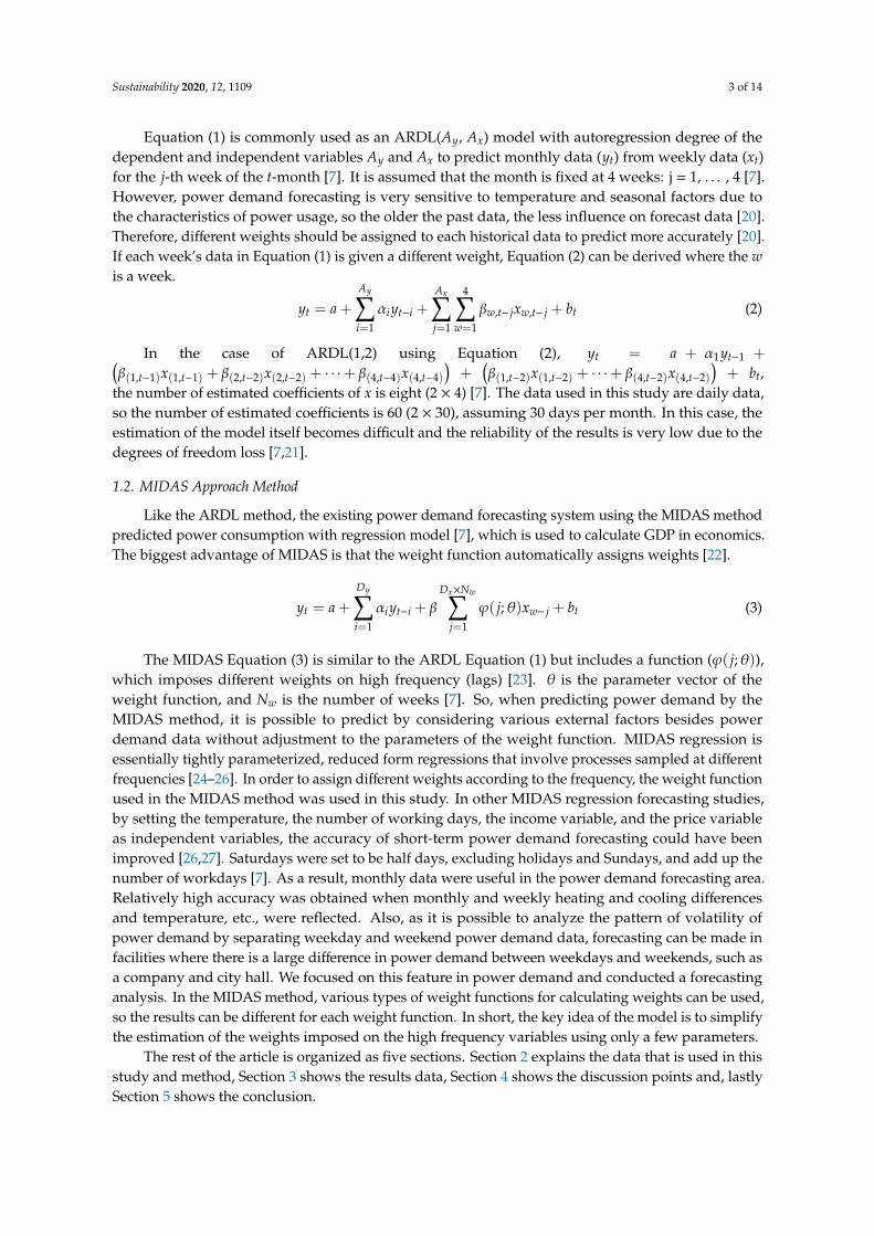
during the previous 12 weeks were used to predict data for the same day during the next four weeks.For example, every Monday, data during the previous 12 weeks was used as train and test data whenthe power demand data for every Monday was predicted during the next four weeks. Likewise, inseasonal data forecast, the previous nine weeks’ 7-day lags data were used to predict the next threeweeks. Figure 3 shows the flowchart of the proposed LSTM structure according to input and outputdata for each of the three models.

Sustainability 2020, 12, 1109 6 of 14

the next week’s data for the same day of the week. In the long-term forecast, twelve 7-day lags data during the previous 12 weeks were used to predict data for the same day during the next four weeks. For example, every Monday, data during the previous 12 weeks was used as train and test data when the power demand data for every Monday was predicted during the next four weeks. Likewise, in seasonal data forecast, the previous nine weeks’ 7-day lags data were used to predict the next three weeks. Figure 3 shows the flowchart of the proposed LSTM structure according to input and output data for each of the three models.

Figure 3. Proposed each LSTM model flowchart when the t is the day.

2.2. Data Preprocessing

Before the previous power demand was entered as input data in the LSTM+MIDAS power demand forecasting model, we performed the preprocessing by assigning different weights to the input data affecting the volatility of the predicted data. Therefore, we conducted preprocessing using MIDAS method’s weight function to weight each day’s worth of input data, which is similar to the volatility of forecasting. 𝒙 = 𝑥 , 𝑥 , 𝑥 , … , 𝑥 is the input previous power demand, which means the power demand at t-th time of nth week’s one day. In the MIDAS method, the weight value is calculated by using the MIDAS regression without directly estimating the weight given to the past value of the information variables. The function to determine the weight for high frequency values using the MIDAS regression method is: 𝒲(𝑛; 𝜃) = exp(𝜃 𝑛 + ⋯ + 𝜃 𝑛)∑ exp(𝜃 𝑛 + ⋯ + 𝜃 𝑛) (4)

The results of the data preprocessing with the above Equation (4) are as follows: 𝑥 = 𝓦𝑥 + 𝑏 (5)

Equation (4) is an ALMOD exponential function, which is widely used as a weighting function of the MIDAS regression method [29–31]. 𝜃 is the parameter vector of the weight function. The shape and speed of the weight function vary depending on the 𝜃 value [7]. We set the 𝜃 value in the range from −0.002 to 0.01 for exponential increase of the weight. 𝓦 is the vector matrix of 𝒲(𝑛; 𝜃) and 𝑏 is a bias coefficient [32]. If the value after the calculation with the weight is too different from the raw data, it is adjusted through the adjustment of the bias value; the bias value is from −0.03 to 4.25.

Figure 3. Proposed each LSTM model flowchart when the t is the day.

2.2. Data Preprocessing

Before the previous power demand was entered as input data in the LSTM+MIDAS powerdemand forecasting model, we performed the preprocessing by assigning different weights to theinput data affecting the volatility of the predicted data. Therefore, we conducted preprocessing usingMIDAS method’s weight function to weight each day’s worth of input data, which is similar to thevolatility of forecasting.

xnt =

{xn

1 , xn2 , xn

3 , . . . , xnt

}is the input previous power demand, which means the power demand

at t-th time of nth week’s one day. In the MIDAS method, the weight value is calculated by using theMIDAS regression without directly estimating the weight given to the past value of the informationvariables. The function to determine the weight for high frequency values using the MIDAS regressionmethod is:

W(n;θ) =exp(θ1n + . . .+ θtn)∑N

i=1 exp(θ1n + . . .+ θtn)(4)

The results of the data preprocessing with the above Equation (4) are as follows:

x′nt = Wxnt + b (5)

Equation (4) is an ALMOD exponential function, which is widely used as a weighting function ofthe MIDAS regression method [29–31]. θ is the parameter vector of the weight function. The shapeand speed of the weight function vary depending on the θ value [7]. We set the θ value in the rangefrom −0.002 to 0.01 for exponential increase of the weight. W is the vector matrix of W(n;θ) and b is abias coefficient [32]. If the value after the calculation with the weight is too different from the raw data,it is adjusted through the adjustment of the bias value; the bias value is from −0.03 to 4.25.

Sustainability 2020, 12, 1109 7 of 14

2.3. LSTM-Based Power Demand Forecasting Model

The LSTM’s forecasting mechanism has been widely used for many time-series forecasting inrecent years [33]. So, we used the LSTM model which is suitable for time-series forecasting, but wemade it possible to reflect the weight function value used in the existing MIDAS to make the model,considering the power demand’s volatility. Figure 4 shows the structure of the LSTM+MIDAS modelfor power demand used in this study.

Sustainability 2020, 12, 1109 7 of 14

2.3. LSTM-Based Power Demand Forecasting Model

The LSTM’s forecasting mechanism has been widely used for many time-series forecasting in recent years [33]. So, we used the LSTM model which is suitable for time-series forecasting, but we made it possible to reflect the weight function value used in the existing MIDAS to make the model, considering the power demand’s volatility. Figure 4 shows the structure of the LSTM+MIDAS model for power demand used in this study.

Figure 4. LSTM+MIDAS model’s structure.

In the LSTM+MIDAS model, the input data 𝑥 from the input layer are entered into the input gates, the forget gates, and the output gates as the parameters. The input parameters’ values are entered by calculation of weight and bias value. At each gate, different values are calculated according to time t. The LSTM structure of the Figure 4 is operated as below: 𝑧 = 𝑔(𝑊 𝒙′ + 𝑅 𝒚 + 𝑏 ) (6)𝑖 = 𝜎(𝑊 𝒙′ + 𝑅 𝒚 + 𝑝 ⊙ 𝑐 + 𝑏 ) (7)𝑓 = 𝜎 𝑊 𝒙′ + 𝑅 𝒚 + 𝑝 ⊙ 𝑐 + 𝑏 (8)𝑐 = 𝑖 ⊙ 𝑧 + 𝑓 ⊙ 𝑐 (9)𝑜 = 𝜎 𝑊 𝒙′ + 𝑅 𝒚 + 𝑝 ⊙ 𝑐 + 𝑏 (10)𝑦 = 𝑜 ⊙ ℎ(𝑐 ) (11)

In the above equations, 𝒙′ and 𝒚 represent the input and output at time t; 𝑖 , 𝑓 , and 𝑜 are the state values of the input gate, forget gate, and output gate; 𝑐 is the state value of the cell at time t; 𝑝 , 𝑝 , and 𝑝 —called peephole connections—are weight vectors connecting the internal memory value of the memory space and the gate; and ⨀ indicates point-wise multiplication. 𝑏 , 𝑏 and 𝑏 are bias values; the W is the input weight matrix; and R is the weight matrix for the input through the circulation.

Figure 4. LSTM+MIDAS model’s structure.

In the LSTM+MIDAS model, the input data x from the input layer are entered into the input gates,the forget gates, and the output gates as the parameters. The input parameters’ values are entered bycalculation of weight and bias value. At each gate, different values are calculated according to time t.The LSTM structure of the Figure 4 is operated as below:

znt = g

(Wzx′nt + Rzyn

t−1 + bz)

(6)

int = σ(Wzx′nt + Rzyn

t−1 + pi � cnt−1 + bi

)(7)

f nt = σ

(W f x′nt + R f yn

t−1 + p f � cnt−1 + b f

)(8)

cnt = int � zn

t + f t� cn

t−1 (9)

ont = σ

(Wox′nt + Royn

t−1 + po � cnt + bo

)(10)

ynt = on

t � h(cn

t

)(11)

In the above equations, x′nt and ynt represent the input and output at time t; int , f n

t , and ont are the

state values of the input gate, forget gate, and output gate; cnt is the state value of the cell at time t; pi, p f ,

and po—called peephole connections—are weight vectors connecting the internal memory value of thememory space and the gate; and � indicates point-wise multiplication. bi, b f and bo are bias values;the W is the input weight matrix; and R is the weight matrix for the input through the circulation.

Sustainability 2020, 12, 1109 8 of 14

2.4. Comparison of Evaluations for Each Model

To evaluate the forecasting performance of LSTM model, we measured the statistical analysisusing the mean relative error, mean absolute percentage error (MAPE), root mean square error (RMSE)and R-squared (R2). The formula for evaluating each model is as follows:

MAPE =100N

N∑i=1

∣∣∣∣∣∣H∗i −Hi

Hi

∣∣∣∣∣∣ (12)

RMSE =

√√√1N

N∑i=1

(H∗i −Hi

)2(13)

R2 = 1−

∑Ni=1

(H∗i −Hi

)2

∑Ni=1

(H −Hi

)2 (14)

where H∗i is the predicted values of the data i, Hi is the actual values of the data i and H is the mean ofHi. The normal range of the R-square is [0, 1], and the closer to 1, the stronger the explanatory powerof the model [6]. Since the power demand data used in this study varies in scale depending on thefacilities, the R2 was calculated to compare the predicted results according to the facilities.

2.5. Development Environment

In this study, we used Deeplearning4J (DL4J) to construct a power demand forecasting modelusing LSTM, which is the one of the most appropriate deep learning-based time series data forecastingmethods [34]. DL4J has a characteristic that it is easy to construct an environment that can use graphicsprocessing unit (GPU). So, we proposed a LSTM model based on the DL4J method combined withMIDAS to optimize for power demand forecasting.

3. Results

3.1. Hyperparameter Setting

The Good performance of deep learning can be achieved by setting the appropriatehyperparameters. The optimal number of layers, nodes, iterations, and activation function, etc.,must be set. Generally, it is necessary to find the most optimal hyperparameter setting according to thenumber or purpose of the data. We found the hyperparameter setting, which achieved optimal resultsthrough a total of 40 settings in the hyperparameter setting. We set the number of hidden layers to 3,the number of nodes to 10, the learning rate to 0.01, and set the number of iterations to 180. We usedhyperbolic tangent (tanh) and stochastic gradient descent as the activation function and optimizationalgorithm of the LSTM layer, respectively. In the classification LSTM model, cross-entropy (CE) andsum of square errors (SSE) are used as cost functions for prediction using multiclass classification, butmean square error (MSE) is predominantly used for prediction using regression [35–37]. Therefore,we used MSE as a cost function to reduce the prediction error. Table 2 shows a total of three resultsshowing the highest accuracy obtained in the experiments to find the optimized hyperparameters.According to each setting, different prediction results were shown, we used Setting 3, which had thehighest accuracy.

Sustainability 2020, 12, 1109 9 of 14

Table 2. The hyperparameter setting value of the LSTM+MIDAS model.

Hyperparameter Setting1 Setting2 Setting3

Hidden layer 2 3 3

The number of nodes 10 8 10

Learning rate 0.001 0.01 0.01

The number of iterations 180 180 180

Activation function Softmax Hyperbolic tangent Hyperbolic tangent

Optimization algorithm Stochastic gradientdescent

Stochastic gradientdescent

Stochastic gradientdescent

Loss function MSE MSE MSE

3.2. Comparison of Experimental Results

Tables 3–5 show the statistical analysis for the experiments conducted in this study by each facilitybuilding. Table 3 is the result of the short-term forecasting and Table 4 is the result of the long-termforecasting. In the case of the short-term forecasting, the MAPE of residential, city hall, factory, hospitalfacilities decreased from 21.04% to 10.44%, from 15.6% to 2.73%, from 7.21% to 1.63%, and from 7.1% to1.96%, respectively. Table 4 shows the long-term forecasting results. There was no significant differencein each error rate by methodology.

Table 3. Error rates of the short-term forecasting results.

Model Index Residential City Hall Factory Hospital

MIDASMAPE (%) 21.040 15.600 7.210 7.100

RMSE 7.940 20.070 46.890 30.930R2 0.302 0.750 0.370 0.926

LSTMMAPE (%) 19.401 4.714 4.060 2.892

RMSE 3.365 7.623 23.302 15.246R2 0.712 0.959 0.830 0.977

LSTM+MIDASMAPE (%) 10.440 2.730 1.630 1.960

RMSE 1.720 7.190 12.510 15.570R2 0.917 0.962 0.893 0.981

Table 4. Error rates of the long-term forecasting results.

Model Index Residential City Hall Factory Hospital

MIDASMAPE (%) 34.610 11.500 7.380 4.040

RMSE 7.950 17.560 59.700 37.070R2 0.416 0.700 0.231 0.891

LSTMMAPE (%) 32.594 9.830 7.710 4.080

RMSE 8.020 17.040 62.130 38.100R2 0.439 0.766 0.235 0.880

LSTM+MIDASMAPE (%) 32.500 8.700 7.700 4.050

RMSE 7.330 14.490 53.610 36.800R2 0.585 0.752 0.248 0.895

Sustainability 2020, 12, 1109 10 of 14

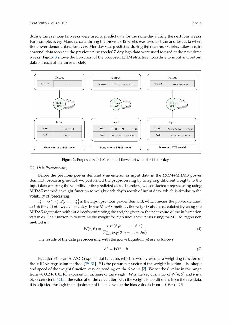
Table 5. Error rates of the residential facility’s seasonal forecasting results.

ModelMAPE (%) RMSE R2

Winter Summer Winter Summer Winter Summer

MIDAS 16.050 10.221 4.632 4.358 0.815 0.729LSTM 16.200 6.520 12.628 2.830 0.094 0.886

LSTM+MIDAS 12.279 5.400 4.400 2.740 0.857 0.896

Table 5 shows the residential facility’s seasonal forecasting results. Unlike the long-term andshort-term forecasting results in Tables 4 and 5, it can be confirmed that the error rates of the largedifference are shown according to the methodology in the case of the experiment of the seasonalforecasting. In the winter experiments, the predicted data included the holiday, which drasticallyreduced the power demand. So, in the MIDAS method, when weighting value was assigned, weexperimented by giving bigger weight to other holiday data. However, in the LSTM method, weight isnot assigned, and thus shows the lowest performance in LSTM as shown in Table 5.

3.3. Statistical Results

LSTM+MIDAS were compared with results from short-term, long-term, and seasonal experimentswith three models (MIDAS, LSTM, LSTM+MIDAS) using a nonparametric statistical test called theFriedman test [38]. The usual form of the Friedman test uses rank instead of the original values, wherethe ranks are obtained by ranking the rows separately and independently from each other [39]. InTable 6, N is the number of our total MAPE results (short-term, long-term, and seasonal), Chi-squaredis 8.6, Degree of freedom (DF) is 2, and the p-value is 0.018. Friedman’s critical value α is set at a 0.05significance level, which has been commonly used in significance level [40].

Table 6. Friedman test results of all forecasting MAPE results.

Friedman Test

N 10Chi-squared 8.6

Degree of freedom (DF) 2p-value 0.018

4. Discussion

In this study, we proposed LSTM+MIDAS, a short-term data optimized power demand forecastingmodel using only the previous power demand data. The accuracy of the power demand forecastingdepends on the data preprocessing, weight function approach. In addition, it is important to set upa model that can closely follow the pattern of power demand volatility over time. In Table 4, weconfirmed that the LSTM+MIDAS model is better reflected in the power demand volatility than theother two methods. As general industrial facilities show similar patterns of power demand every day,short-term power demand forecasting using our model was very efficient. On the other hand, facilitybuildings that tend to respond sensitively to weekend and weather influences, such as residential,should be seasonally classified and then applied to our LSTM+MIDAS model.

To sum up the experiment’s results, we confirmed the lowest forecasting performance forresidential facilities, whereas the factory and hospital facilities showed a high accuracy with a relativelylow level of error rates. The LSTM+MIDAS model of short-term data showed a higher level offorecasting than the other two methodologies. Also, the results of the short-term data are relativelybetter than those of the long-term data. We confirmed that, in comparison with the largest MAPEin the case of short-term forecasting, our LSTM+MIDAS model shows that the residential facilitiesdecreased by 10.44%p, city hall by 12.87%p, factories by 5.58%p, and hospitals by 5.14%p; in the case oflong-term forecasting, residential facilities only decreased by 2.11%p and city hall by 2.8%p. Long-term

Sustainability 2020, 12, 1109 11 of 14

forecasting did not improve the error rates in power demand forecasting at factories and hospitalfacilities. Generally, the power demand forecasting using the short-term data more accurately reflectsthe volatility, thereby improving the accuracy of short-term forecasting. However, the prediction oflong-term data is highly influenced by weather and external factors, so the accuracy of the methodologydoes not show much difference, even though the overall accuracy is higher due to the larger number ofdatasets. We confirmed that there was no improvement in accuracy according to the methodology inthe long-term power demand forecasting. Because the power demand data is related to the volatility,the long-term power demand data is not well predicted at the time of the volatility trends.

We also confirmed that predictions of power demand in residential facilities that are sensitive toweather, seasonal, and holiday influences can achieve higher accuracy by seasonally categorizing andpredicting the data considering the weights for special situations, as shown in Figure 5.

Sustainability 2020, 12, 1109 11 of 14

We also confirmed that predictions of power demand in residential facilities that are sensitive to weather, seasonal, and holiday influences can achieve higher accuracy by seasonally categorizing and predicting the data considering the weights for special situations, as shown in Figure 5.

Figure 5. Residential seasonal power demand 3-day forecasting represented in 6-h intervals.

Other existing Cheng et al.’s study on power demand forecasting for residential facilities using PowerLSTM was used for July power demand input data [41]. We also used July data for summer forecasts, so we compared residential power demand forecasts for summer and Cheng et al.’s study [41]. The results show a comparison of the MAPE values of our model and Cheng et al.’s PowerLSTM model using residential data [41]. The MAPE of our LSTM+MIDAS is 5.400%, and the PowerLSTM is 8.935%. The difference is 3.535%p and the error rate (MAPE) of LSTM+MIDAS is reduced by 39.564% compared to PowerLSTM [41]. In addition, we conducted the Friedman test to show whether the LSTM+MIDAS model is more meaningful than the MIDAS or LSTM model for the values of each experiment. We identified that the LSTM+MIDAS model is less than the α (p < 0.05). So, we can say that the LSTM+MIDAS model results are statistically significant through the Friedman test.

5. Conclusions

The existing power demand forecasting method using the regression analysis method required many external factors, in addition to the previous power demand data. However, in this study, it is possible to predict the power demand with reduced error rates only by the previous power demand data using the prediction of the patterns’ trends. We could analyze that predicted power demand patterns were different depending on the facilities. Especially, residential facilities are very influenced by the seasonal factors. Since we considered only power demand data as input data, the forecasting error rate of residential facilities, which is affected by the weather, increased more than other facilities. The analysis of other factors affecting power demand can be added to predict power demand performances.

So, this study can be expected to further future studies, provide efficient and accurate forecasting of power demand by adding data on external factors affecting power demand predicting, as well as

Figure 5. Residential seasonal power demand 3-day forecasting represented in 6-h intervals.

Other existing Cheng et al.’s study on power demand forecasting for residential facilities usingPowerLSTM was used for July power demand input data [41]. We also used July data for summerforecasts, so we compared residential power demand forecasts for summer and Cheng et al.’s study [41].The results show a comparison of the MAPE values of our model and Cheng et al.’s PowerLSTMmodel using residential data [41]. The MAPE of our LSTM+MIDAS is 5.400%, and the PowerLSTM is8.935%. The difference is 3.535%p and the error rate (MAPE) of LSTM+MIDAS is reduced by 39.564%compared to PowerLSTM [41]. In addition, we conducted the Friedman test to show whether theLSTM+MIDAS model is more meaningful than the MIDAS or LSTM model for the values of eachexperiment. We identified that the LSTM+MIDAS model is less than the α (p < 0.05). So, we can saythat the LSTM+MIDAS model results are statistically significant through the Friedman test.

5. Conclusions

The existing power demand forecasting method using the regression analysis method requiredmany external factors, in addition to the previous power demand data. However, in this study,

Sustainability 2020, 12, 1109 12 of 14

it is possible to predict the power demand with reduced error rates only by the previous powerdemand data using the prediction of the patterns’ trends. We could analyze that predicted powerdemand patterns were different depending on the facilities. Especially, residential facilities are veryinfluenced by the seasonal factors. Since we considered only power demand data as input data, theforecasting error rate of residential facilities, which is affected by the weather, increased more thanother facilities. The analysis of other factors affecting power demand can be added to predict powerdemand performances.

So, this study can be expected to further future studies, provide efficient and accurate forecastingof power demand by adding data on external factors affecting power demand predicting, as well asprevious power demand data. In addition, predicting accurate power demand with high performancewould be contributed to the sustainable development of the natural environment and environmentmanagement area, which are nowadays great issues all over the world.

Author Contributions: Writing—original draft preparation, E.C.; writing—review and editing, E.C. and D.K.K.;data curation, S.C. All authors have read and agreed to the published version of the manuscript.

Funding: This research received no external funding.

Acknowledgments: This work was supported by the Korea Institute of Energy Technology Evaluation andPlanning(KETEP) and the Ministry of Trade, Industry & Energy(MOTIE) of the Republic of Korea (No.2018201060010C).

Conflicts of Interest: The authors declare no conflict of interest.

References

1. Jang, B.J.; Han, S.G. Energy-IT Fusion Technology Trends and Major Issues. JOK 2010, 28, 44–51.2. Yang, E.S.; Kim, A.R.; Kim, B.A.; Shin, B.R. World Energy Outlook (WEO-2017) and Changes in Energy

Demand and Supply. 2017. Available online: http://www.keei.re.kr/keei/download/WEIS1703.pdf (accessedon 4 December 2019).

3. Sung, M.J.; Shin, K.W. A Small-area Hardware Implementation of EGML-based Moving Object DetectionProcessor. JKIICE 2017, 21, 2213–2220.

4. Eum, J.Y. A Study on the Development of Energy Supply and Demand Forecasting Models for Smart CityEnergy Management System (CEMS). Master’s Thesis, Sangmyung University, Seoul, Korea, 2015.

5. Zhang, B.; Pu, Y.; Wang, Y.; Li, J. Forecasting hotel accommodation demand based on LSTM modelincorporating internet search index. Sustainability 2019, 11, 4708. [CrossRef]

6. Luo, T. Research on Decision-Making of Complex Venture Capital Based on Financial Big Data Platform.Complexity 2018, 2018, 5170281. [CrossRef]

7. Kim, C.H. Power Demand Forecasting Model Using Mixed Cycle Data. Research Report. 2014. Availableonline: http://www.keei.re.kr/web_keei/d_results.nsf/0/6632BB5F39AB536C49257E0D001A2348/$file/%EA%B8%B0%EB%B3%B8%202014-06%20%ED%98%BC%ED%95%A9%EC%A3%BC%EA%B8%B0%20%EC%9E%90%EB%A3%8C%EB%A5%BC%20%EC%9D%B4%EC%9A%A9%ED%95%9C%20%EC%A0%84%EB%A0%A5%EC%88%98%EC%9A%94%20%EC%98%88%EC%B8%A1%20%EB%AA%A8%ED%98%95%20%EA%B5%AC%EC%B6%95.pdf (accessed on 10 December 2019).

8. Majd, M.; Safabakhsh, R. Correlational Convolutional LSTM for Human Action Recognition. Neurocomputing.In Press. Available online: https://www.sciencedirect.com/science/article/abs/pii/S0925231219304436(accessed on 10 December 2019).

9. Bhadbhade, N.; Yilmaz, S.; Zuberi, S.J.; Eichhammer, W. The evolution of energy efficiency in Switzerland inthe period 2000-2016. Energy 2020, 191, 116526. [CrossRef]

10. IEA. Insights Brief: Energy Efficiency Targets. Available online: https://webstore.iea.org/insights-brief-energy-efficiency-targets (accessed on 28 January 2020).

11. Jo, N.H. SVM Load Forecasting using Cross-Validation. Trans. Korean. Inst. Elect. Eng. 2006, 55A, 485–491.12. Ishikawa, S.; Iwabuchi, K.; Takano, J. Peak power demand leveling to stabilize and reduce the power demand

of dairy barn. Eng. Agric. Environ. Food 2016, 9, 56–63. [CrossRef]13. Tang, R.; Li, H.; Wang, S. A game theory-based decentralized control strategy for power demand management

of building cluster using thermal mass and energy storage. Appl. Energy 2019, 242, 809–820. [CrossRef]

Sustainability 2020, 12, 1109 13 of 14

14. Rivera-González, L.; Bolonio, D.; Mazadiego, L.F.; Valencia-Chapi, R. Long-Term Electricity Supply andDemand Forecast (2018–2040): A LEAP Model Application towards a Sustainable Power Generation Systemin Ecuador. Sustainability 2019, 11, 5316. [CrossRef]

15. Lee, J.Y.; Kolasani, L. Security Based Network for Health Care System. APJCRI 2015, 1, 1–6. [CrossRef]16. Law, R.; Li, G.; Fong, D.K.C.; Han, X. Tourism Demand Forecasting: A Deep Learning Approach. Ann. Tour.

Res. 2019, 75, 410–423. [CrossRef]17. Xu, P.; Du, R.; Zhang, Z. Predicting Pipeline Leakage in Petrochemical System through GAN and LSTM.

Knowl. Based Syst. 2019, 175, 50–61. [CrossRef]18. Petersen, N.C.; Rodrigues, F.; Pereira, F.C. Multi-output bus travel time forecasting with convolutional LSTM

neural network. Expert Syst. Appl. 2019, 120, 426–435. [CrossRef]19. Mohsen, B.O.; Ferda, H.; Scott, W.H. Mexican Bilateral Trade and the J-curve: An Application of the Nonlinear

ARDL Model. Econ. Anal. Policy 2016, 50, 23–40.20. Fousekis, P.; Katrakilidis, C.; Trachanas, E. Vertical Price Transmission in the US Beef Sector: Evidence from

the Nonlinear ARDL Model. Econ. Model 2016, 52, 499–506. [CrossRef]21. Li, T. A (3,2) reduced degree-of-freedom unified zigzag laminated beam theory. Appl. Math. Model. 2020, 77,

1474–1496. [CrossRef]22. Won, H.N.; Choi, K.W.; Choi, B.J. Forecasting GDP with a Mixed Data Sampling Model. IEJ 2016, 22, 83–117.23. Mei, D.; Ma, F.; Liao, Y.; Wang, L. Geopolitical risk uncertainty and oil future volatility: Evidence from

MIDAS models. Energy Econ. 2020, 86, 104624. [CrossRef]24. Ghysels, E.; Qian, H. Estimating MIDAS Regressions via OLS with Polynomial Parameter Profiling. Econ.

Stat. 2019, 9, 1–16. [CrossRef]25. Andreou, E. On the Use of High Frequency Measures of Volatility in MIDAS Regressions. J. Econ. 2016, 193,

367–389. [CrossRef]26. Zhou, Z.; Fu, Z.; Jiang, Y.; Zeng, X.; Lin, L. Can Economic Policy Uncertainty Predict Exchange Rate

Volatility? New Evidence from the GARCH-MIDAS Model. Finance Res. Lett. In press. Available online:https://www.sciencedirect.com/science/article/abs/pii/S1544612319304982 (accessed on 28 January 2020).

27. He, Y.; Lin, B. Forecasting China’s total energy demand and its structure using ADL-MIDAS model. Energy2018, 151, 420–429. [CrossRef]

28. Seo, D.H.; Lyu, J.; Choi, E.J.; Cho, S.; Kim, D.K. Web based Customer Power Demand Variation EstimationSystem using LSTM. JKIICE 2018, 22, 587–594.

29. Ghyselsa, E.; Clarab, P.S.; Valkanovb, R. Predicting volatility: Getting the most out of return data sampled atdifferent frequencies. J. Econ. 2006, 131, 59–95. [CrossRef]

30. Barndorff-Nielsen, O.E.; Corcuera, J.M.; Podolskij, M. Power variation for Gaussian processes with stationaryincrements. Stoch. Process. Their Appl. 2009, 119, 1845–1865. [CrossRef]

31. Barndorff-Nielsen, O.E.; Shephard, N. Power and bipower variation with stochastic volatility and jumps(with discussion). J. Financ. Econ. 2004, 2, 1–48.

32. Li, Y.; Han, C. Prediction for Tourism Flow based on LSTM Neural Network. Procedia Comput. Sci. 2018, 129,277–283. [CrossRef]

33. Sideratos, G.; Ikonomopoulos, A.; Hatziargyriou, D.N. A novel fuzzy-based ensemble model for loadforecasting using hybrid deep neural networks. Electr. Pow Syst. Res. 2020, 178, 106025. [CrossRef]

34. Eclipse Deeplearning4j. Available online: https://deeplearning4j.org/about (accessed on 11 December 2019).35. Peimankar, A.; Sadasivan, P. An Ensemble of Deep Recurrent Neural Networks for P-wave Detection in

Electrocardiogram. In Proceedings of the ICASSP 2019-2019 IEEE International Conference on Acoustics,Speech and Signal Processing (ICASSP), Brighton, UK, 12–17 May 2019; IEEE: Piscataway, NJ, USA, 2019.Available online: https://ieeexplore.ieee.org/document/8682307 (accessed on 4 February 2020).

36. Goki, S. Deep Learning from Scratch, 1st ed.; Hanbit Media: Seoul, Korea, 2017; pp. 111–112.37. Goki, S. Deep Learning from Scratch 2, 1st ed.; Hanbit Media: Seoul, Korea, 2019; pp. 40–41.38. Peimankar, A.; Weddell, S.J.; Jalal, T.; Lapthorn, A.C. Multi-objective ensemble forecasting with an application

to power transformers. Appl. Soft Comput. 2018, 68, 233–248. [CrossRef]39. Rohmel, J. The permutation distribution of the Friedman test. Comput. Stat. Data Anal. 1997, 26, 83–99.

[CrossRef]40. Demsar, J. Statistical comparisons of classifiers over multiple data sets. J. Mach. Learn. Res. 2006, 7, 1–30.

Sustainability 2020, 12, 1109 14 of 14

41. Cheng, Y.; Xu, C.; Mashima, D.; Thing, L.L.V.; Wu, Y. PowerLSTM: Power Demand Forecasting Using LongShort-Term Memory Neural Network. In Advanced Data Mining and Applications: 13th International Conference,Singapore, 5–6 November 2017; Springer: Berlin, Germany, 2017; Available online: https://link.springer.com/

chapter/10.1007/978-3-319-69179-4_51 (accessed on 4 February 2020).

© 2020 by the authors. Licensee MDPI, Basel, Switzerland. This article is an open accessarticle distributed under the terms and conditions of the Creative Commons Attribution(CC BY) license (http://creativecommons.org/licenses/by/4.0/).