Power-aware scheduling for periodic real-time tasks ...people.cs.pitt.edu/~melhem/vita/doc/01275298.pdfPower-Aware Scheduling for Periodic Real-Time Tasks Hakan Aydin, Member, IEEE

Power-Aware Scheduling forPeriodic Real-Time Tasks

Hakan Aydin, Member, IEEE Computer Society, Rami Melhem, Fellow, IEEE,

Daniel Mosse, Member, IEEE Computer Society, and

Pedro Mejıa-Alvarez, Member, IEEE Computer Society

Abstract—In this paper, we address power-aware scheduling of periodic tasks to reduce CPU energy consumption in hard real-time

systems through dynamic voltage scaling. Our intertask voltage scheduling solution includes three components: 1) a static (offline)

solution to compute the optimal speed, assuming worst-case workload for each arrival, 2) an online speed reduction mechanism to

reclaim energy by adapting to the actual workload, and 3) an online, adaptive and speculative speed adjustment mechanism to

anticipate early completions of future executions by using the average-case workload information. All these solutions still guarantee

that all deadlines are met. Our simulation results show that our reclaiming algorithm alone outperforms other recently proposed

intertask voltage scheduling schemes. Our speculative techniques are shown to provide additional gains, approaching the theoretical

lower-bound by a margin of 10 percent.

Index Terms—Real-time systems, power-aware computing, low-power systems, dynamic voltage scaling, periodic task scheduling.

�

1 INTRODUCTION

IN the last decade, the research community has addressedlow-power system design problems with a multidimen-

sional effort. Reducing the energy consumption of acomputer system has necessarily multiple aspects, invol-ving separate components such as CPU, memory system,and I/O subsystem. Hardware and software manufacturershave agreed to introduce standards such as the ACPI(Advanced Configuration and Power Interface) [10] forpower management of laptop computers that allows severalmodes of operation, such as predictive system shutdown.An obvious target for energy reduction is the processor: Anearly study found that 18-30 percent of the total energyconsumption is due to the CPU alone [17]. More recentreports show that this fraction can exceed 50 percent forCPU-intensive workloads [24], [31]. Dynamic voltage scaling(DVS) framework, which involves dynamically adjustingthe voltage and frequency to reduce CPU power consump-tion, has recently become a major research area.

In fact, the power consumption of an on-chip system is a

strictly increasing convex function of the supply voltage Vdd,

but its exact form depends on the technology. For example,

the dominant component of energy consumption in widely

popular CMOS technology is the dynamic power dissipation

Pd, which is given by Pd ¼ Ceff � V 2dd � f , where Ceff is the

effective switched capacitance and f is the frequency of the

clock. On the other hand, the gate delay D is inversely

related to the supply voltage Vdd as given by the formula

D ¼ k � Vdd

ðVdd�VtÞ2, where k is a constant and Vt is the threshold

voltage. From these equations, it can be seen that one can

obtain striking power savings if the supply voltage and the

clock frequency are reduced simultaneously. Thus, the

dynamic voltage scaling technique (known also as variable

voltage scheduling) is based on obtaining energy savings by

simultaneously reducing the supply voltage and the clock

frequency, at the expense of increased latency. The exact

form of the power/speed relation can be obtained by

resorting to normalization: recent research studies [9], [11],

[14], [15] report formulas where the CPU power consump-

tion per cycle when expressed in terms of CPU speed is a

polynomial of the third degree. In general, this relation can

be captured by strictly increasing convex functions. Systems

which are able to operate on a (more or less) continuous

voltage spectrum are rapidly becoming a reality thanks to

advances in power-supply electronics and CPU design [6],

[21]. For example, the Crusoe processor is able to

dynamically adjust clock frequency in 33 MHz steps [28].For systems with timing constraints and scarce energy

resources, we solve the Real-Time Dynamic Voltage Scaling(RT-DVS) problem: adjust the supply voltage and clockfrequency to minimize CPU energy consumption whilestill meeting the deadlines. First, task speed assignmentsthat minimize the energy consumption for the worst-caseworkload should be evaluated at the static level. However,limiting RT-DVS with this static solution would be veryconservative: Real-time applications usually exhibit large

584 IEEE TRANSACTIONS ON COMPUTERS, VOL. 53, NO. 5, MAY 2004

. H. Aydin is with the Computer Science Department, George MasonUniversity, Fairfax, VA 22030. E-mail: [email protected].

. R. Melhem and D. Mosse are with the Computer Science Department,University of Pittsburgh, Pittsburgh, PA 15260.E-mail: {melhem, mosse}@cs.pitt.edu.

. P. Mejıa-Alvarez is with CINVESTAV-IPN, Seccion de Computacion, Av.I.P.N. 2508, Zacatenco, Mexico, DF 07300.E-mail: [email protected].

Manuscript received 21 Nov. 2001; revised 27 Feb. 2003; accepted 26 Aug.2003.For information on obtaining reprints of this article, please send e-mail to:[email protected], and reference IEEECS Log Number 115429.

0018-9340/04/$20.00 � 2004 IEEE Published by the IEEE Computer Society

variations in the actual workload experienced by the system;for example, [4] reports that the ratio of the worst-caseexecution time to the best-case execution time can be ashigh as 10 in typical applications. Thus, at the second,reclaiming level, dynamically monitoring task executionsand further reducing CPU speed by reallocating unusedCPU time can provide additional savings. Finally, we canconsider the speculation level where early task completionsare anticipated and the CPU speed is aggressively reduced.However, it is imperative that all these components bedesigned not to cause any deadlines to be missed evenunder a worst-case workload that can happen after anyspeed adjustment point.

1.1 Related Work

The work by Weiser et al. [29] was among the first topropose (and evaluate the performance of) various DVSalgorithms, though the focus of that study was non-real-time tasks. Yao et al. [30] provided a static, optimal, andpolynomial-time scheduling algorithm for real-time taskswith release times and deadlines, assuming aperiodic tasksand worst-case execution times. Pering and Brodersen [22]also addressed the static dimension of RT-DVS, but only foraperiodic tasks. Static solutions for extended/hybrid taskmodels were addressed in various papers: Heuristics foronline scheduling of aperiodic tasks while not hurting thefeasibility of periodic requests are proposed in [8]. The samepaper also suggested that the CPU speed be set to theutilization of the periodic tasks’ utilization value in theabsence of aperiodic tasks, but without mentioning orproving the optimality of this choice. Nonpreemptivepower-aware scheduling is investigated in [7]. Concentrat-ing on periodic task sets with identical periods, the effectsof having an upper bound on the voltage change rate areexamined in [9], along with a heuristic to solve the problem.

The possible variations in actual workload of real-timesystems and, hence, reclaiming and speculation dimensionsattracted the attention of power management researchcommunity first in the late 1990s. These dynamic algo-rithms, according to an established classification [5], [12],[26] fall either into intertask or intratask DVS algorithmcategories. In the former case, speed assignments aredetermined at task-level: Though dynamic adjustmentsare performed, these occur only at task dispatch orcompletion times. That is, once a task is assigned CPU,the CPU speed is not changed until it is preempted orcompleted. On the other hand, intratask algorithms adjustspeed within the boundaries of a given task; typically, thespeed is gradually increased to assure the timely comple-tion. Intratask algorithms usually require some degree ofcompiler support to insert power management points into theapplication code, in order to call explicitly OperatingSystem services for speed reduction. On the other hand,intertask algorithms do not involve such changes at theapplication code and, thus, they are more practical.

In the intratask DVS research, Lorch and Smith addressedthe scheduling of aperiodic tasks with soft deadlines in [18].Shin et al. [26] proposed an intratask DVS framework foraperiodic real-time tasks with (possibly) precedence con-straints. Gruian [5] provided an intratask DVS algorithm forperiodic tasks scheduled according to the Rate-Monotonicpolicy.

Among the intertask DVS algorithms, an early techniquebased on slowing down the processor whenever there is asingle task eligible for execution is given in [27]. Dynamicenergy reclaiming issues (without speculation) in power-aware scheduling were addressed [13] for cyclic andperiodic task models in the context of systems with two(discrete) voltage levels. To the best of our knowledge, theconcept of “speculative speed reduction” was first intro-duced by the authors in [20]; however, only tasks sharing acommon deadline were considered. A recent study parti-cularly relevant for the settings of this paper is due to Pillaiand Shin [23], where the authors proposed a reclaimingalgorithm (Cycle-Conserving EDF) and a speculation-basedalgorithm (Look-Ahead EDF). These intertask DVS algo-rithms are based on updating and predicting the instanta-neous utilization of the periodic task set. Finally, a recentperformance evaluation [12] compares several intertask andintratask DVS algorithms in their own categories, includingthe preliminary versions of some algorithms discussed inthis paper.

1.2 Paper Organization and Contributions

In this paper, we address three dimensions of intertaskdynamic voltage scaling algorithms for periodic real-timetask systems, assuming that the CPU speed can be variedover a continuous spectrum between a lower bound and anupper bound. We develop novel algorithms and evaluatetheir performance against other intertask DVS algorithmsproposed in the literature, as well as against the provablyoptimal, clairvoyant algorithm whose performance pro-vides a lower bound for any (inter or intratask) DVSalgorithm. Thus, we present:

1. A static (offline) solution to compute the optimalspeed at the task level, assuming worst-case work-load for each arrival1 (Section 3).

2. A generic dynamic reclaiming algorithm for tasksthat complete without consuming their worst-caseworkload (Section 4). Our reclaiming algorithmdiffers from other intertask reclaiming algorithms(e.g., CC-EDF in [23]) in that it attempts to allocatethe maximum (possibly, the entire) amount ofunused CPU time (slack) to the first task at theappropriate priority level, in a greedy fashion. Further,when preempted, tasks implicitly return the slackthey inherited to the favor of the newly dispatchedtask. We formally prove that the tasks will still meettheir deadlines if the speed is reduced according tothe rules we provide upon early completions. Weachieve these objectives by keeping track of theremaining execution times of tasks in the staticoptimal schedule, in which each task instance presentsits worst-case workload.

3. An online, adaptive, and speculative speed adjust-ment mechanism to anticipate and compensateprobable early completion of future executions(Section 5). We explore two intertwined questionsraised by the speculative component, namely, a) thelevel of aggressiveness that justifies speculative speed

AYDIN ET AL.: POWER-AWARE SCHEDULING FOR PERIODIC REAL-TIME TASKS 585

1. Due to the nature of DVS, the actual execution time is dependent onthe CPU speed and, therefore, the worst-case number of required CPUcycles is a more appropriate measure of the worst-case workload (seeSection 2).

reductions under a given probability distribution ofthe actual workload and b) the issue of guaranteeingthe timing constraints even in aggressive modes.Our aggressive algorithms differ from other inter-task speculation-based algorithms (e.g., LA-EDF in[23]) by reducing exclusively the speed of thedispatched task, at the expense of borrowing CPUtime from other ready tasks. Further, the algorithmsare still able to reclaim the available slack (if any)and we show that the feasibility is preserved evenafter speculative speed reductions. The aggressive-ness level of these algorithms can be adjusted by thedesigner. In fact, our results indicate that a balancedaggressiveness level that aims to achieve the speedthat corresponds to the expected workload gives thebest results.

Through extensive simulations, we compare our reclaim-ing and aggressive algorithms against other state-of-the-artintertask DVS algorithms, as well as the lower-bound thatcan be achieved by any (intra or inter) DVS algorithm(Section 6). We experimentally show that the dynamicreclaiming algorithm alone provides higher energy savingsthan other existing techniques. Moreover, our aggressivealgorithms yield additional gains, approaching the theore-tical lower bound by a margin of 10 percent.

Finally, in Section 7, we address additional considera-tions such as the applicability to platforms with discretespeed levels and the consequences of using quadraticpower/speed functions. We underline that our objective isto minimize CPU energy consumption; low-power techni-ques for memory, disk, and I/O subsystems, albeitimportant, are beyond the scope of this paper.

2 SYSTEM MODEL AND NOTATION

The ready time and deadline of each real-time task Ti willbe denoted by ri and di, respectively. The indicator of theworst-case workload in variable voltage/speed settings,that is, the worst-case number of processor cycles requiredby Ti, will be denoted by Ci. Note that, under a constantspeed S (given in cycles per second), the execution time ofthe task Ti is ti ¼ Ci

S . A schedule of real-time tasks is said tobe feasible if each task Ti receives at least ACi CPU cyclesbefore its deadline, where ACi � Ci is the actual number ofCPU cycles (actual workload) of Ti.

We assume that the CPU speed can be changed con-tinuously between a minimum speed Smin (that correspondsto theminimum supply voltage necessary to keep the systemfunctional) and amaximum speed Smax. We also assume that0 � Smin � Smax ¼ 1, that is, we normalize the speed valueswith respect to Smax. In our framework, the voltage/speedchanges take place only at context switch time andwhile statesaving instructions execute. Pouwelse et al. report in [24] thatthe voltage/speed change can be performed in less than 140�s in Strong ARM SA-1100 processor. If not negligible, the“voltage change overhead” can be incorporated into theworst-case workload of each task.

We assume that the process descriptor of the task Ti hastwo extra fields related to speed settings, in addition toother conventional fields. The first one, Si, denotes thecurrent CPU speed at which Ti is executing. The other fieldbSiSi denotes the nominal speed of Ti, which is the indicator of

the “default” speed of Ti. For each dispatched task, theoperating system sets Si ¼ bSiSi, prior to any dynamic speedadjustment.

Thepowerconsumptionof theprocessorunder thespeedSis given by gðSÞ, which is assumed to be a strictly increasingconvex function, represented by a polynomial of at leastseconddegree [9]. If the task Ti occupies the processor duringthe time interval ½t1; t2�, then the energy consumed by CPUduring this interval is Eðt1; t2Þ ¼

R t2t1gðSðtÞÞdt. We consider

only CPU power/energy consumption in this paper.In our detailed analysis of periodic power-aware

scheduling, we will consider a set T ¼ fT1; . . . ; Tng ofn periodic real-time tasks. The period of Ti is denoted byPi, which is also equal to the deadline of the currentinvocation. We refer to the jth invocation of task Ti as Ti;j.All tasks are assumed to be independent and ready at t ¼ 0.Hence, the ready time of Ti;j is ri;j ¼ ðj� 1Þ � Pi and itsdeadline is di;j ¼ j � Pi.

We define Utot as the total utilization of the task set undermaximum speed Smax ¼ 1, that is, Utot ¼

Pni¼1

Ci

Pi. Note that

the schedulability theorems for periodic real-time tasks [16]imply that Utot � 1:0 is a necessary condition to have at leastone feasible schedule; hence, throughout the paper, we willassume that Utot ¼

Pni¼1

Ci

Pi� 1.

3 OPTIMAL STATIC SOLUTION

In this section, we present the static optimal solution to thevariable voltage scheduling problem for the periodic taskmodel, assuming that each task presents its worst-case workload tothe processor at every instance. We show that the speed valuewhich minimizes the total energy consumption correspondsto the utilization of the system subject to the minimum CPUspeed constraint. We underline that, in [2], solving aninstance of the RT-DVS problem is shown to be equivalent tosolving an instance of Reward-Based Scheduling (RBS)problem with concave reward functions [1], [3]. Further, theequivalenceofRBSandRT-DVS ispreserved regardlessof thetask model (aperiodic/periodic or preemptive/nonpreemp-tive), as long as our aim is to reach a solution for a given(worst-case) workload under timing constraints [2]. Thismeans that solutionsdevised for theRBSproblemcanbeusedfor the RT-DVS problem.However, one can also compute thestatic optimal speed for periodic task sets by using the firstprinciples as outlined below.

Proposition 1. The optimal speed to minimize the total energyconsumption while meeting all the deadlines is constant andequal to �SS ¼ maxfSmin; Utotg. Moreover, when used alongwith this speed �SS, any periodic hard real-time policy which canfully utilize the processor (e.g., Earliest Deadline First, LeastLaxity First) can be used to obtain a feasible schedule.

Proof. First, observe that the convex nature of the power-speed function suggests that we should try to maintain auniform speedwhile fully utilizing theCPU to the extent itis possible. If Utot � Smin, then using the speed �SS ¼ Utot

leads clearly to a schedule which is fully utilized (i.e., noidle time), through stretching out each task in equalproportions (in other words, in this case, we are achievinga total effective task utilization of

Pni¼1

Ci�SS�Pi

¼ Utot�SS¼ 1). Note

that stretching out each task in equal proportionsguarantees the optimality, thanks to the convexity of


power consumption function gðSÞ (see [2] for a formalproof). However, if Utot < Smin, then we should use theminimum CPU speed available to stretch out taskexecutions as much as possible. In any case, using thespeed �SS ¼ maxfSmin; Utotg will result in a total effectivetask utilization which is no greater than 1. Hence, anyscheduling policy which can achieve up to 100 percentCPU utilization (Earliest Deadline First, Least LaxityFirst) can be used to complete all the task instancesbefore their deadlines with the speed �SS. tu

4 DYNAMIC RECLAIMING ALGORITHM

Though the static scheme can be shown to be optimal undera worst-case workload, it is known that, in many cases, theinstances of real-time tasks complete earlier than under theworst-case scenario [4]. A trivial remedy would be to shutdown the processor when there are no ready tasks.However, this technique is clearly suboptimal because ofthe convexity of the power consumption function: It isalways more energy-efficient to transfer unused CPU timeto other tasks by reducing their speeds whenever possible.

The dynamic reclaiming algorithm we present in thissection is based on detecting early completions andadjusting (reducing) the speed of other tasks on-the-fly inorder to provide additional power savings while stillmeeting the deadlines. To this aim, we perform compar-isons between the actual execution history and thecanonical schedule Scan, which is the static optimal schedulein which every instance presents its worst-case workload tothe processor and runs at the constant speed �SS. The CPUspeed is adjusted only at task dispatch times: Thus, weshould be able to say whether the task is being dispatchedearlier than under Scan and, if so, determine the amount ofadditional CPU time the dispatched task can safely use toslow down its execution; we will refer to this additionalCPU time as the earliness of the dispatched task.

Before providing the details of our approach, we under-line that a simple approach that equates earliness withpreviously unused CPU time and blindly slows down theprocessor is not a safe approach. To see this, consider a3-task system with the following parameters:

C1 ¼ 4; P1 ¼ 10; C2 ¼ 4; P2 ¼ 10; C3 ¼ 6; P3 ¼ 30:

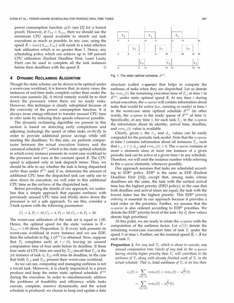
The worst-case utilization of the task set is equal to 1.00.Hence, the optimal speed for the static version is �SS ¼Smax ¼ 1:00 (from Proposition 1). If every task presents itsworst-case workload at every instance and we use EDF,then the schedule in Fig. 1 (Scan) is obtained. Now, supposethat T3 completes early at t ¼ 10, leaving an unusedcomputation time of four units before its deadline. If thesefour units of CPU time are used by T1;2 (recall that Ti;j is thejth instance of task i), T2;2 will miss its deadline, in the casethat both T1;2 and T2;2 present their worst-case workload.

As we can see, computing and managing earliness is nota trivial task. Moreover, it is clearly impractical to a prioriproduce and keep the entire static optimal schedule Scan

during the execution. In order to simultaneously addressthe problems of feasibility and efficiency while tasksexecute, complete, rearrive dynamically and the actualschedule is produced, we choose to keep and update a data

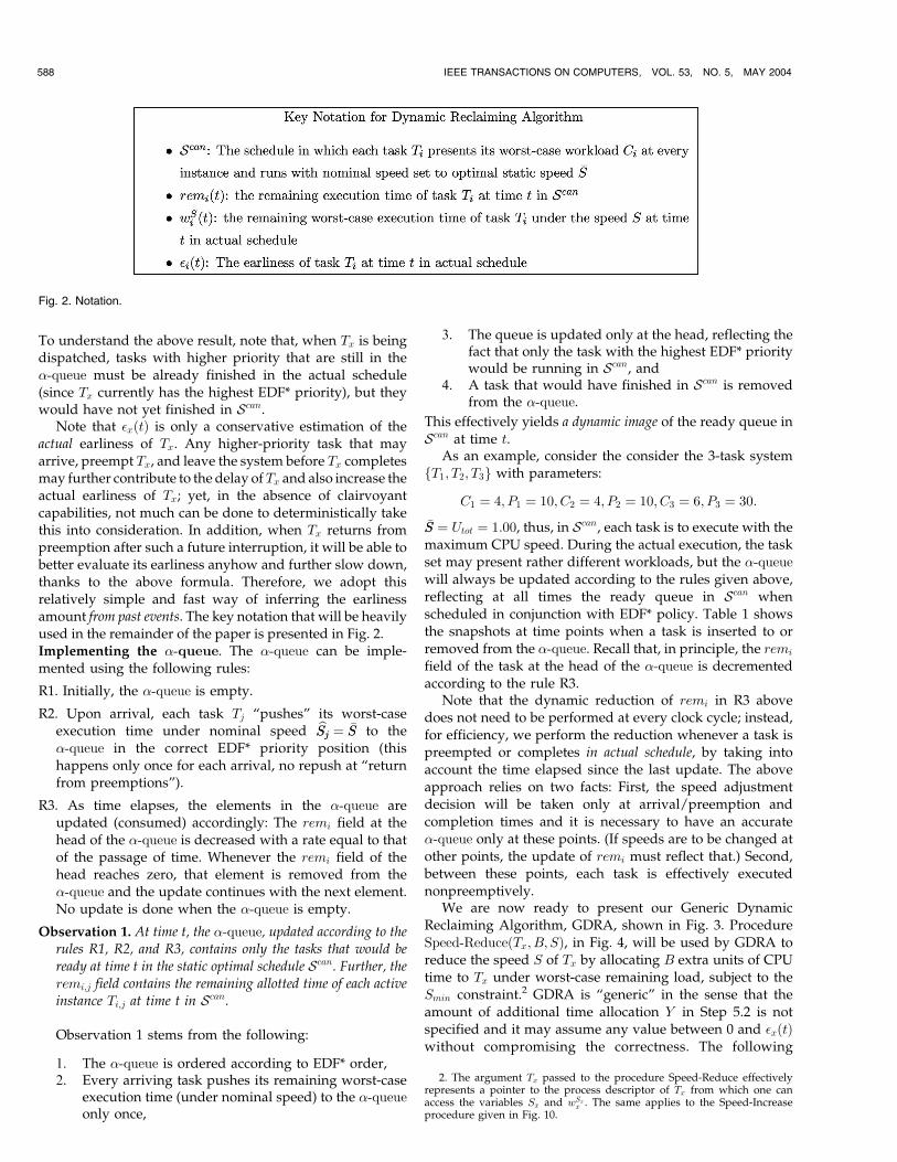
structure (called �-queue) that helps to compute theearliness of tasks when they are dispatched. Let us denoteby remi;jðtÞ the remaining execution time of Ti;j at time t inScan, under static optimal speed �SS. At any time t duringactual execution, the �-queue will contain information abouttasks that would be active (i.e., running or ready) at time tin the worst-case static optimal schedule Scan (in otherwords, the �-queue is the ready queue of Scan at time t).Specifically, at any time t, for each task Ti;j in the �-queuethe information about its identity, arrival time, deadline,and remi;jðtÞ value is available.

Clearly, given t, the ri;j and di;j values can be easilycomputed for the periodic task model. Note that the �-queueat time t contains information about all instances Ti;j suchthat ri;j � t � di;j, and remi;jðtÞ > 0. The �-queue contains atmost n elements since at most one instance of a givenperiodic task can be active at a given time t in any schedule.Therefore, we will omit the instance number while referringto the �-queue elements, whenever possible.

Our approach assumes that tasks are scheduled accord-ing to EDF* policy. EDF* is the same as EDF (EarliestDeadline First [16]), except that, among tasks whosedeadlines are the same, the task with the earliest arrivaltime has the highest priority (FIFO policy); in the case thatboth deadline and arrival times are equal, the task with thelowest index has the highest priority. This EDF* priorityordering is essential in our approach because it provides atotal order on the priorities. Further, we assume that the�-queue is also ordered according to EDF* priorities. Wedenote the EDF* priority-level of the task i by d�i (low valuesdenote high priorities).

At this point, we are ready to relate the �-queue with thecomputation of the earliness factor. Let wS

i ðtÞ denote theremaining worst-case execution time of task Ti under thespeed S at time t. Further, set the nominal speed bSiSi ¼ �SS foreach task Ti.

Proposition 2. For any task Tx which is about to execute, anyunused computation time (slack) of any task in the �-queuehaving strictly higher priority than Tx will contribute to theearliness of Tx along with already finished work of Tx in theactual schedule. That is, total earliness of Tx is no less than

�xðtÞ ¼X

ijd�i <d�x

remiðtÞ þ remxðtÞ � wbSxSxx ðtÞ

¼X

ijd�i�d�x

remiðtÞ � wbSxSxx ðtÞ:


Fig. 1. The static optimal schedule, Scan.

To understand the above result, note that, when Tx is beingdispatched, tasks with higher priority that are still in the�-queue must be already finished in the actual schedule(since Tx currently has the highest EDF* priority), but theywould have not yet finished in Scan.

Note that �xðtÞ is only a conservative estimation of theactual earliness of Tx. Any higher-priority task that mayarrive, preempt Tx, and leave the system before Tx completesmay further contribute to the delay ofTx and also increase theactual earliness of Tx; yet, in the absence of clairvoyantcapabilities, not much can be done to deterministically takethis into consideration. In addition, when Tx returns frompreemption after such a future interruption, it will be able tobetter evaluate its earliness anyhow and further slow down,thanks to the above formula. Therefore, we adopt thisrelatively simple and fast way of inferring the earlinessamount from past events. The key notation that will be heavilyused in the remainder of the paper is presented in Fig. 2.Implementing the �-queue. The �-queue can be imple-mented using the following rules:

R1. Initially, the �-queue is empty.

R2. Upon arrival, each task Tj “pushes” its worst-caseexecution time under nominal speed bSjSj ¼ �SS to the�-queue in the correct EDF* priority position (thishappens only once for each arrival, no repush at “returnfrom preemptions”).

R3. As time elapses, the elements in the �-queue areupdated (consumed) accordingly: The remi field at thehead of the �-queue is decreased with a rate equal to thatof the passage of time. Whenever the remi field of thehead reaches zero, that element is removed from the�-queue and the update continues with the next element.No update is done when the �-queue is empty.

Observation 1. At time t, the �-queue, updated according to therules R1, R2, and R3, contains only the tasks that would beready at time t in the static optimal schedule Scan. Further, theremi;j field contains the remaining allotted time of each activeinstance Ti;j at time t in Scan.

Observation 1 stems from the following:

1. The �-queue is ordered according to EDF* order,2. Every arriving task pushes its remaining worst-case

execution time (under nominal speed) to the �-queueonly once,

3. The queue is updated only at the head, reflecting thefact that only the task with the highest EDF* prioritywould be running in Scan, and

4. A task that would have finished in Scan is removedfrom the �-queue.

This effectively yields a dynamic image of the ready queue inScan at time t.

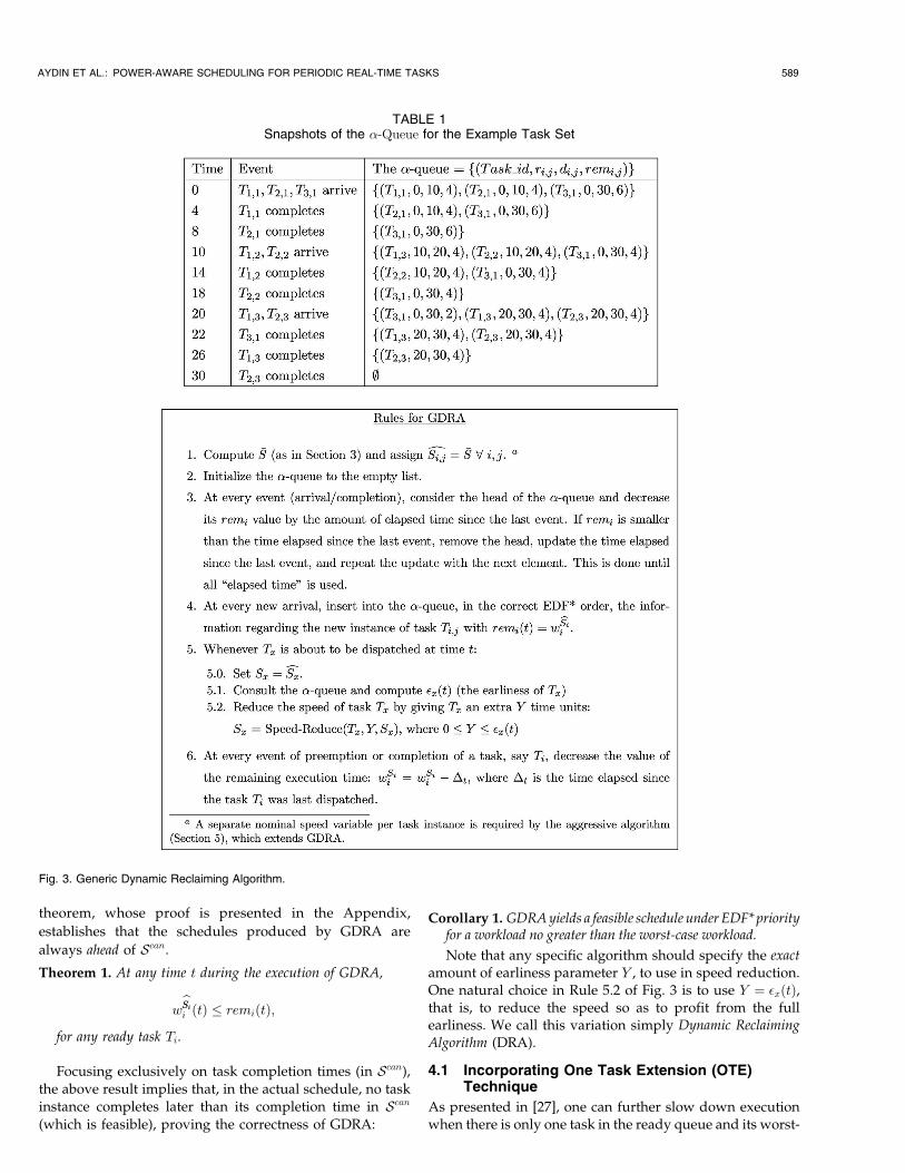
As an example, consider the consider the 3-task systemfT1; T2; T3g with parameters:

C1 ¼ 4; P1 ¼ 10; C2 ¼ 4; P2 ¼ 10; C3 ¼ 6; P3 ¼ 30:

�SS ¼ Utot ¼ 1:00, thus, in Scan, each task is to execute with themaximum CPU speed. During the actual execution, the taskset may present rather different workloads, but the �-queue

will always be updated according to the rules given above,reflecting at all times the ready queue in Scan whenscheduled in conjunction with EDF* policy. Table 1 showsthe snapshots at time points when a task is inserted to orremoved from the �-queue. Recall that, in principle, the remi

field of the task at the head of the �-queue is decrementedaccording to the rule R3.

Note that the dynamic reduction of remi in R3 abovedoes not need to be performed at every clock cycle; instead,for efficiency, we perform the reduction whenever a task ispreempted or completes in actual schedule, by taking intoaccount the time elapsed since the last update. The aboveapproach relies on two facts: First, the speed adjustmentdecision will be taken only at arrival/preemption andcompletion times and it is necessary to have an accurate�-queue only at these points. (If speeds are to be changed atother points, the update of remi must reflect that.) Second,between these points, each task is effectively executednonpreemptively.

We are now ready to present our Generic DynamicReclaiming Algorithm, GDRA, shown in Fig. 3. ProcedureSpeed-ReduceðTx;B; SÞ, in Fig. 4, will be used by GDRA toreduce the speed S of Tx by allocating B extra units of CPUtime to Tx under worst-case remaining load, subject to theSmin constraint.2 GDRA is “generic” in the sense that theamount of additional time allocation Y in Step 5.2 is notspecified and it may assume any value between 0 and �xðtÞwithout compromising the correctness. The following


Fig. 2. Notation.

2. The argument Tx passed to the procedure Speed-Reduce effectivelyrepresents a pointer to the process descriptor of Tx from which one canaccess the variables Sx and wSx

x . The same applies to the Speed-Increaseprocedure given in Fig. 10.

theorem, whose proof is presented in the Appendix,

establishes that the schedules produced by GDRA are

always ahead of Scan.

Theorem 1. At any time t during the execution of GDRA,

wbSiSi

i ðtÞ � remiðtÞ;

for any ready task Ti.

Focusing exclusively on task completion times (in Scan),

the above result implies that, in the actual schedule, no taskinstance completes later than its completion time in Scan

(which is feasible), proving the correctness of GDRA:

Corollary 1. GDRA yields a feasible schedule under EDF* priorityfor a workload no greater than the worst-case workload.

Note that any specific algorithm should specify the exactamount of earliness parameter Y , to use in speed reduction.One natural choice in Rule 5.2 of Fig. 3 is to use Y ¼ �xðtÞ,that is, to reduce the speed so as to profit from the fullearliness. We call this variation simply Dynamic ReclaimingAlgorithm (DRA).

4.1 Incorporating One Task Extension (OTE)Technique

As presented in [27], one can further slow down executionwhen there is only one task in the ready queue and its worst-


TABLE 1Snapshots of the �-Queue for the Example Task Set

Fig. 3. Generic Dynamic Reclaiming Algorithm.

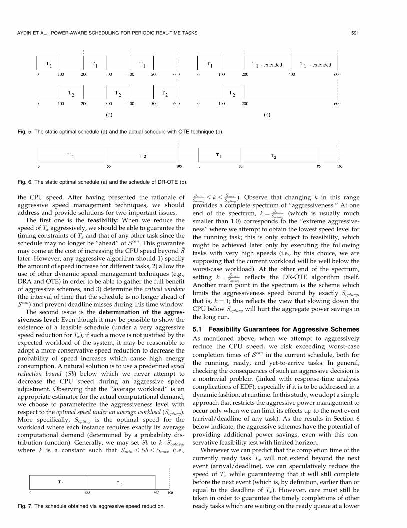
case completion time (under the current speed) does notextend beyond the next event (next arrival/closest deadline ofany task). For example, consider the following 2-task system:C1 ¼ 100; P1 ¼ 200; C2 ¼ 300; P2 ¼ 600. Again, it is easy tosee that �SS ¼ Smax ¼ 1:00. The worst-case static schedule Scan

is shown in Fig. 5a.In the actual execution, suppose that the schedule follows

Scan until t ¼ 200 and T2 completes early at t ¼ 200.When thesecond instance of T1 arrives at t ¼ 200, the �-queue has the2-instance snapshot fðT1;2; 200; 400; 100Þ; ðT2;1; 0; 600; 200Þg.Note that, even though T2 completed, rem2ð200Þ is still200 since the updating of the �-queue only reduced it by100 units. At this point (t ¼ 200), the earliness �1ð200Þ ¼ 0and DRA would not reduce the speed. But, we can actuallyreduce the speed S1 safely to 0.5, effectively adding theinterval ½300; 400� for the execution of T1;2 and ½500; 600� forthe execution of T1;3 (see Fig. 5b). Observe that, at t1 ¼ 100,T2 is also the only ready task and its earliness �2ð100Þ ¼ 0,yet it cannot reduce its speed since t1 þ wS2

2 > 200 which isthe time of the next event.

OTE technique can be used in conjunction with anyscheduling policy: To improve (G)DRA, we add a newrule 5.3. Let NTA be the next arrival time of any taskinstance in the system after t and recall that Sx is the speedfrom Step 5.2 in (G)DRA and t is the time Tx is dispatched.

5.3. IfTx is theonly ready taskandZ ¼ NTA� t� wSxx ðtÞ > 0,

set Sx ¼ Speed-ReduceðTx; Z; Sx)

In other words, reduce the speed of Tx so as to use the idleCPU up to time NTA. We call this improved technique DR-OTE. Clearly, the following holds.

Proposition 3. If all the task instances meet their deadlines underDRA, they will also meet their deadlines under the algorithmDR-OTE.

5 AGGRESSIVE SPEED REDUCTION

The DRA and DR-OTE algorithms provide sound dynamicspeed reclaiming mechanisms, however, they guaranteefeasibility by always being “ahead” of the static worst-caseoptimal schedule Scan (i.e., tasks never actually start orfinish after the scheduled time in Scan). Scan is feasible at alltimes, yet it is optimal only under the assumption that allfuture instances will present their worst-case workload.Whenever, under constant speed, the actual execution timesof a task’s instances exhibit large variation, starting a taskwith this assumption can be too conservative. Instead,whenever the current system state suggests, we mayassume speculatively that the current and future instances

will most probably present a computational demand

which is lower than the worst case. Hence, we can adoptan “aggressive” approach based on reducing the speed of

the running task under certain conditions to a level which iseven lower than the one suggested by DR-OTE. But, thisspeculative move might shift the task’s worst-case comple-tion time to a point later than the one in Scan under an actualhigh workload. And, if this pessimistic scenario turns out tobe true, we should be ready to increase the CPU speedbeyond �SS later to guarantee feasibility of future tasks.This would hamper significant power savings since theconvexity of power/speed curve suggests a uniform speedto achieve a given average speed value over any interval oftime. On the other hand, in the case that the actualworkload turns out to be lower than the worst case, theactual schedule will still be ahead of Scan, even with the lowspeed, thereby achieving even higher power savings.

Let us illustrate the aggressive scheme by a simpleexample, in which we have C1 ¼ C2 ¼ 25, P1 ¼ P2 ¼ 100,gðSÞ ¼ S3. The static worst-case optimal schedule Scan

(Fig. 6a) is obtained by computing �SS ¼ Utot ¼ 0:5. Note thatScan is optimal only when the actual required CPU cyclesACi ¼ Ci for i ¼ 1; 2, for which case the total energyconsumption is E1 ¼ 50ð0:5Þ3 þ 50ð0:5Þ3 ¼ 12:5. In case thatAC1 < C1 and/or AC2 < C2, Scan is no longer optimal. Forexample, if AC1 ¼ 15 and AC2 ¼ 20, then starting with �SSand applying the DR-OTE algorithm yields the scheduleshown in Fig. 6b.

Note that, because of its actual lowworkload,T1 completesat t ¼ 30. Then, the DR-OTE algorithm is able to dynamicallyreclaim unused 20 units of time, effectively reducing S2 to25

50þ20 ¼ 2570 ¼ 0:35. But, sinceAC2 < C2, T2 also completes well

before thedeadline. In this case, the total energy consumptionis3 E2 ¼ 30ð0:5Þ3 þ 56ð0:35Þ3 þ 14ð0:1Þ3 ¼ 6:16. However, byadopting an aggressive scheme, we can start to execute T1

with a speed lower than S1 ¼ 0:50, for example, S1 ¼ 0:35.In this case, T1 will complete at t ¼ 42:8 and the dynamicreclaiming algorithm will further set S2 to

2550þ7:2 ¼ 25

57:2 ¼ 0:43(note that we cannot, at this point, set the speed S2 anylower than this and still guarantee completion within thedeadline). T2 will complete at t ¼ 42:8þ 20

0:43 ¼ 89:3. Theschedule is depicted in Fig. 7. The total energy consumptionin this aggressive scheme is

42:8ð0:35Þ3 þ 46:5ð0:43Þ3 þ 10:7ð0:1Þ3 ¼ 5:54275;

providing an additional 10 percent in power savings withrespect to DR-OTE.

However, we should point out that, under a verypessimistic scenario where AC1 ¼ C1, the aggressivescheme would have to execute T2 with high speed toprevent a deadline miss, resulting in a high energyconsumption. We conclude this example by noting that itwould not be possible to “aggressively” assign a speedlower than 25

75 ¼ 0:33 to S1 since doing so and having aworst-case workload for T1 might result in a deadline missfor T2, even under S2 ¼ Smax.

A powerful system design principle is to make thecommon case more efficient. This translates (in settingswhere the worst-case workload occurs only rarely) intohaving a power-efficient schedule for average or close toaverage cases, which can be achieved by further reducing


3. Note that we are using the minimum CPU speed Smin ¼ 0:1 in theinterval ½86; 100�.

Fig. 4. Speed Reduction Procedure.

the CPU speed. After having presented the rationale ofaggressive speed management techniques, we shouldaddress and provide solutions for two important issues.

The first one is the feasibility: When we reduce thespeed of Tx aggressively, we should be able to guarantee thetiming constraints of Tx and that of any other task since theschedule may no longer be “ahead” of Scan. This guaranteemay come at the cost of increasing the CPU speed beyond �SSlater. However, any aggressive algorithm should 1) specifythe amount of speed increase for different tasks, 2) allow theuse of other dynamic speed management techniques (e.g.,DRA and OTE) in order to be able to gather the full benefitof aggressive schemes, and 3) determine the critical window(the interval of time that the schedule is no longer ahead ofScan) and prevent deadline misses during this time window.

The second issue is the determination of the aggres-siveness level: Even though it may be possible to show theexistence of a feasible schedule (under a very aggressivespeed reduction for Tx), if such a move is not justified by theexpected workload of the system, it may be reasonable toadopt a more conservative speed reduction to decrease theprobability of speed increases which cause high energyconsumption. A natural solution is to use a predefined speedreduction bound (Sb) below which we never attempt todecrease the CPU speed during an aggressive speedadjustment. Observing that the “average workload” is anappropriate estimator for the actual computational demand,we choose to parameterize the aggressiveness level withrespect to the optimal speed under an average workload (Soptavg).More specifically, Soptavg is the optimal speed for theworkload where each instance requires exactly its averagecomputational demand (determined by a probability dis-tribution function). Generally, we may set Sb to k � Soptavg,where k is a constant such that Smin � Sb � Smax (i.e.,

Smin

Soptavg� k � Smax

Soptavg). Observe that changing k in this range

provides a complete spectrum of “aggressiveness.” At one

end of the spectrum, k ¼ Smin

Soptavg(which is usually much

smaller than 1.0) corresponds to the “extreme aggressive-

ness” where we attempt to obtain the lowest speed level for

the running task; this is only subject to feasibility, which

might be achieved later only by executing the following

tasks with very high speeds (i.e., by this choice, we are

supposing that the current workload will be well below the

worst-case workload). At the other end of the spectrum,

setting k ¼ Smax

Soptavgreflects the DR-OTE algorithm itself.

Another main point in the spectrum is the scheme which

limits the aggressiveness speed bound by exactly Soptavg,

that is, k ¼ 1; this reflects the view that slowing down the

CPU below Soptavg will hurt the aggregate power savings in

the long run.

5.1 Feasibility Guarantees for Aggressive Schemes

As mentioned above, when we attempt to aggressively

reduce the CPU speed, we risk exceeding worst-case

completion times of Scan in the current schedule, both for

the running, ready, and yet-to-arrive tasks. In general,

checking the consequences of such an aggressive decision is

a nontrivial problem (linked with response-time analysis

complications of EDF), especially if it is to be addressed in a

dynamic fashion, at runtime. In this study,we adopt a simple

approach that restricts the aggressive power management to

occur only when we can limit its effects up to the next event

(arrival/deadline of any task). As the results in Section 6

below indicate, the aggressive schemes have the potential of

providing additional power savings, even with this con-

servative feasibility test with limited horizon.Whenever we can predict that the completion time of the

currently ready task Tx will not extend beyond the next

event (arrival/deadline), we can speculatively reduce the

speed of Tx while guaranteeing that it will still complete

before the next event (which is, by definition, earlier than or

equal to the deadline of Tx). However, care must still be

taken in order to guarantee the timely completions of other

ready tasks which are waiting on the ready queue at a lower


Fig. 6. The static optimal schedule (a) and the schedule of DR-OTE (b).

Fig. 7. The schedule obtained via aggressive speed reduction.

Fig. 5. The static optimal schedule (a) and the actual schedule with OTE technique (b).

priority level than Tx, since the execution/completion ofthese tasks will be delayed until Tx completes.

A possible way to guarantee the feasibility in this case isto increase the speed of another suitable and ready task Ty

which will run after Tx. This is effectively equivalent toincreasing the time allocation of Tx, while decreasing thetime allocation of Ty by the same amount. Clearly, from thispoint on, the system cannot blindly decrease the speed of Ty

to its original bSySy (i.e., we should also change bSySy for thatinstance).

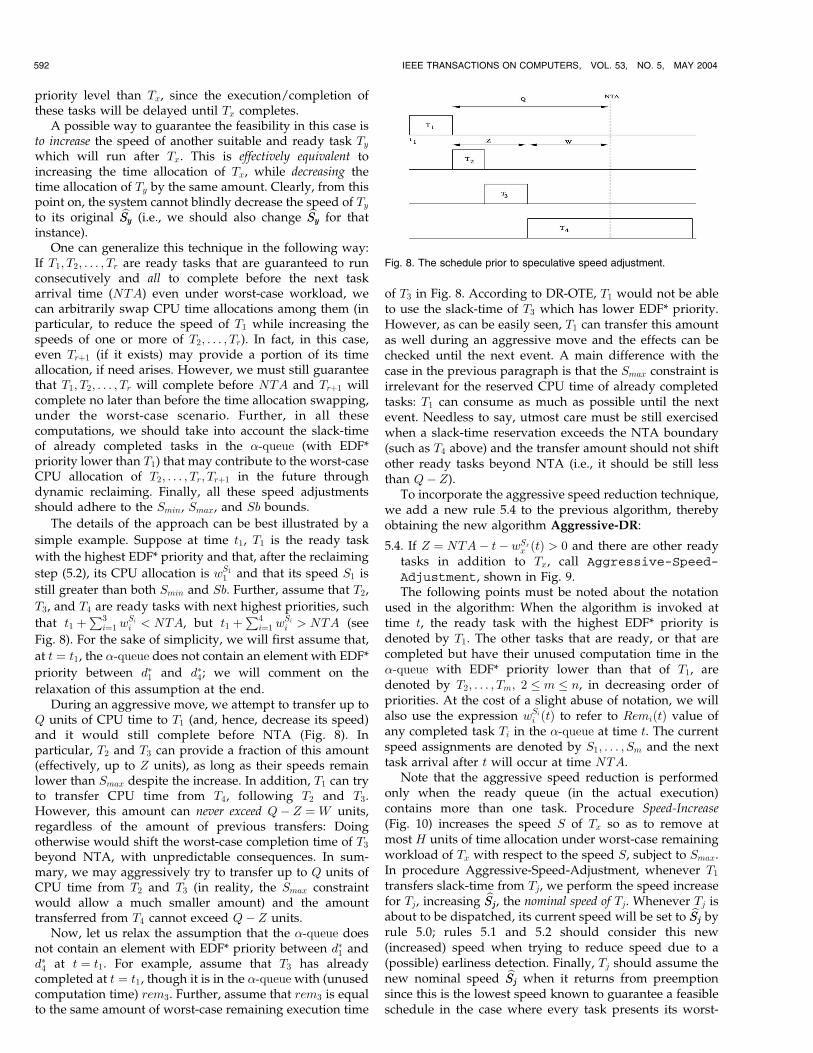
One can generalize this technique in the following way:If T1; T2; . . . ; Tr are ready tasks that are guaranteed to runconsecutively and all to complete before the next taskarrival time (NTA) even under worst-case workload, wecan arbitrarily swap CPU time allocations among them (inparticular, to reduce the speed of T1 while increasing thespeeds of one or more of T2; . . . ; Tr). In fact, in this case,even Trþ1 (if it exists) may provide a portion of its timeallocation, if need arises. However, we must still guaranteethat T1; T2; . . . ; Tr will complete before NTA and Trþ1 willcomplete no later than before the time allocation swapping,under the worst-case scenario. Further, in all thesecomputations, we should take into account the slack-timeof already completed tasks in the �-queue (with EDF*priority lower than T1) that may contribute to the worst-caseCPU allocation of T2; . . . ; Tr; Trþ1 in the future throughdynamic reclaiming. Finally, all these speed adjustmentsshould adhere to the Smin, Smax, and Sb bounds.

The details of the approach can be best illustrated by a

simple example. Suppose at time t1, T1 is the ready task

with the highest EDF* priority and that, after the reclaiming

step (5.2), its CPU allocation is wS1

1 and that its speed S1 is

still greater than both Smin and Sb. Further, assume that T2,

T3, and T4 are ready tasks with next highest priorities, such

that t1 þP3

i¼1 wSi

i < NTA, but t1 þP4

i¼1 wSi

i > NTA (see

Fig. 8). For the sake of simplicity, we will first assume that,

at t ¼ t1, the �-queue does not contain an element with EDF*

priority between d�1 and d�4; we will comment on the

relaxation of this assumption at the end.During an aggressive move, we attempt to transfer up to

Q units of CPU time to T1 (and, hence, decrease its speed)and it would still complete before NTA (Fig. 8). Inparticular, T2 and T3 can provide a fraction of this amount(effectively, up to Z units), as long as their speeds remainlower than Smax despite the increase. In addition, T1 can tryto transfer CPU time from T4, following T2 and T3.However, this amount can never exceed Q� Z ¼ W units,regardless of the amount of previous transfers: Doingotherwise would shift the worst-case completion time of T3

beyond NTA, with unpredictable consequences. In sum-mary, we may aggressively try to transfer up to Q units ofCPU time from T2 and T3 (in reality, the Smax constraintwould allow a much smaller amount) and the amounttransferred from T4 cannot exceed Q� Z units.

Now, let us relax the assumption that the �-queue doesnot contain an element with EDF* priority between d�1 andd�4 at t ¼ t1. For example, assume that T3 has alreadycompleted at t ¼ t1, though it is in the �-queuewith (unusedcomputation time) rem3. Further, assume that rem3 is equalto the same amount of worst-case remaining execution time

of T3 in Fig. 8. According to DR-OTE, T1 would not be ableto use the slack-time of T3 which has lower EDF* priority.However, as can be easily seen, T1 can transfer this amountas well during an aggressive move and the effects can bechecked until the next event. A main difference with thecase in the previous paragraph is that the Smax constraint isirrelevant for the reserved CPU time of already completedtasks: T1 can consume as much as possible until the nextevent. Needless to say, utmost care must be still exercisedwhen a slack-time reservation exceeds the NTA boundary(such as T4 above) and the transfer amount should not shiftother ready tasks beyond NTA (i.e., it should be still lessthan Q� Z).

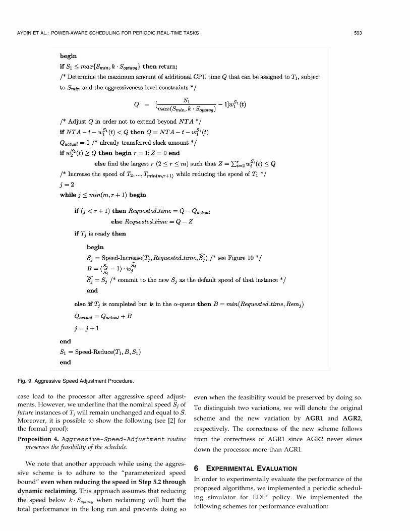
To incorporate the aggressive speed reduction technique,we add a new rule 5.4 to the previous algorithm, therebyobtaining the new algorithm Aggressive-DR:

5.4. If Z ¼ NTA� t� wSxx ðtÞ > 0 and there are other ready

tasks in addition to Tx, call Aggressive-Speed-

Adjustment, shown in Fig. 9.The following points must be noted about the notation

used in the algorithm: When the algorithm is invoked attime t, the ready task with the highest EDF* priority isdenoted by T1. The other tasks that are ready, or that arecompleted but have their unused computation time in the�-queue with EDF* priority lower than that of T1, aredenoted by T2; . . . ; Tm; 2 � m � n, in decreasing order ofpriorities. At the cost of a slight abuse of notation, we willalso use the expression wSi

i ðtÞ to refer to RemiðtÞ value ofany completed task Ti in the �-queue at time t. The currentspeed assignments are denoted by S1; . . . ; Sm and the nexttask arrival after t will occur at time NTA.

Note that the aggressive speed reduction is performedonly when the ready queue (in the actual execution)contains more than one task. Procedure Speed-Increase(Fig. 10) increases the speed S of Tx so as to remove atmost H units of time allocation under worst-case remainingworkload of Tx with respect to the speed S, subject to Smax.In procedure Aggressive-Speed-Adjustment, whenever T1

transfers slack-time from Tj, we perform the speed increasefor Tj, increasing bSjSj, the nominal speed of Tj. Whenever Tj isabout to be dispatched, its current speed will be set to bSjSj byrule 5.0; rules 5.1 and 5.2 should consider this new(increased) speed when trying to reduce speed due to a(possible) earliness detection. Finally, Tj should assume thenew nominal speed bSjSj when it returns from preemptionsince this is the lowest speed known to guarantee a feasibleschedule in the case where every task presents its worst-


Fig. 8. The schedule prior to speculative speed adjustment.

case load to the processor after aggressive speed adjust-

ments. However, we underline that the nominal speed bSjSj of

future instances of Tj will remain unchanged and equal to �SS.

Moreover, it is possible to show the following (see [2] for

the formal proof):

Proposition 4. Aggressive-Speed-Adjustment routine

preserves the feasibility of the schedule.

We note that another approach while using the aggres-

sive scheme is to adhere to the “parameterized speed

bound” even when reducing the speed in Step 5.2 through

dynamic reclaiming. This approach assumes that reducing

the speed below k � Soptavg when reclaiming will hurt the

total performance in the long run and prevents doing so

even when the feasibility would be preserved by doing so.

To distinguish two variations, we will denote the original

scheme and the new variation by AGR1 and AGR2,

respectively. The correctness of the new scheme follows

from the correctness of AGR1 since AGR2 never slows

down the processor more than AGR1.

6 EXPERIMENTAL EVALUATION

In order to experimentally evaluate the performance of the

proposed algorithms, we implemented a periodic schedul-

ing simulator for EDF* policy. We implemented the

following schemes for performance evaluation:


Fig. 9. Aggressive Speed Adjustment Procedure.

. Static uses constant speed �SS and switches to power-down mode (i.e., S ¼ Smin) whenever there is noready task.

. OTE: Static optimal speed scheme in conjunctionwith One Task Extension (but without dynamicreclaiming).

. CC-EDF (Cycle-conserving EDF): the reclaimingalgorithm proposed by Pillai and Shin ([23]).

. LA-EDF (Look-ahead EDF): the speculative algo-rithm proposed by Pillai and Shin ([23]).

. DRA, which is implemented in two variations: withor without the OTE technique (DR-OTE and DRA,respectively).

. AGR1 with the parameterized speed bound set toSoptavg (i.e., the aggressiveness factor k is set to 1).

. AGR2 with the parameterized speed bound set to0:9 � Soptavg (i.e., the aggressiveness factor k is set to0:9).4

. Bound, which is the clairvoyant algorithm thatknows the exact actual workload in advance andadopts an optimal speed accordingly.5

In our experiments, we investigated the average perfor-

mance of the schemes over a large spectrum of worst-case

utilization (Utot) and variability in the actual workload. In

particular, we first focused on the average energy con-sumption of 100 task sets, each containing 30 tasks. We

repeated the experiments for 20 and 10-task sets as well.

The periods of the tasks were chosen randomly in theinterval ½1;000; 32;000�. The minimum speed Smin is set to

0.1. The nominal speed �SS is set to Utot, as the optimality of

this choice was shown in Section 3. The variability in the

actual workload is achieved by modifying the WCETBCET ratio

(that is, the worst-case to the best-case execution time ratio).

We ran experiments where the actual execution time

follows a normal or uniform probability distributionfunction. In the case of the normal distribution, the mean

and the standard deviation are set to WCETþBCET2 and

WCET�BCET6 , respectively, for a given WCET

BCET , as suggested in

[27]. The choice of this mean and standard deviationensures that, on the average, 99.7 percent of the execution

times fall in the interval ½BCET;WCET �. In the case of the

uniform distribution, the mean is again set to WCETþBCET2 .

For each task set, we simulated the execution 10 times in

interval [0, LCM], where LCM is the Least Common

Multiple of P1; . . . ; Pn, and we measured the average energyconsumption per experiment using a cubic power/speedfunction [9], [11], [14], [15]. To investigate the effect of thespecific form of the convex power consumption function,we also performed experiments with quadratic power/speed function. We comment on the results of this last set ofexperiments in Section 7.

6.1 General Trends

One remarkable outcome of the experimental evaluation is

the following: Although the OTE scheme provides sub-

stantial improvements over techniques that continuously

use Smax during the execution without reclaiming [27],

throughout the entire spectrum, DR-OTE only provides a

marginal (less than 1 percent) improvement over pure DRA.

This result indicates that almost the entire power savings

are obtained by initially committing to �SS, which fully

utilizes the CPU (Static), and using the dynamic reclaiming

algorithm itself. To improve the readability of the graphs,

we show below only the results of DR-OTE since the results

for the latter are almost identical to the pure DRA. The same

observation holds for CC-EDF.

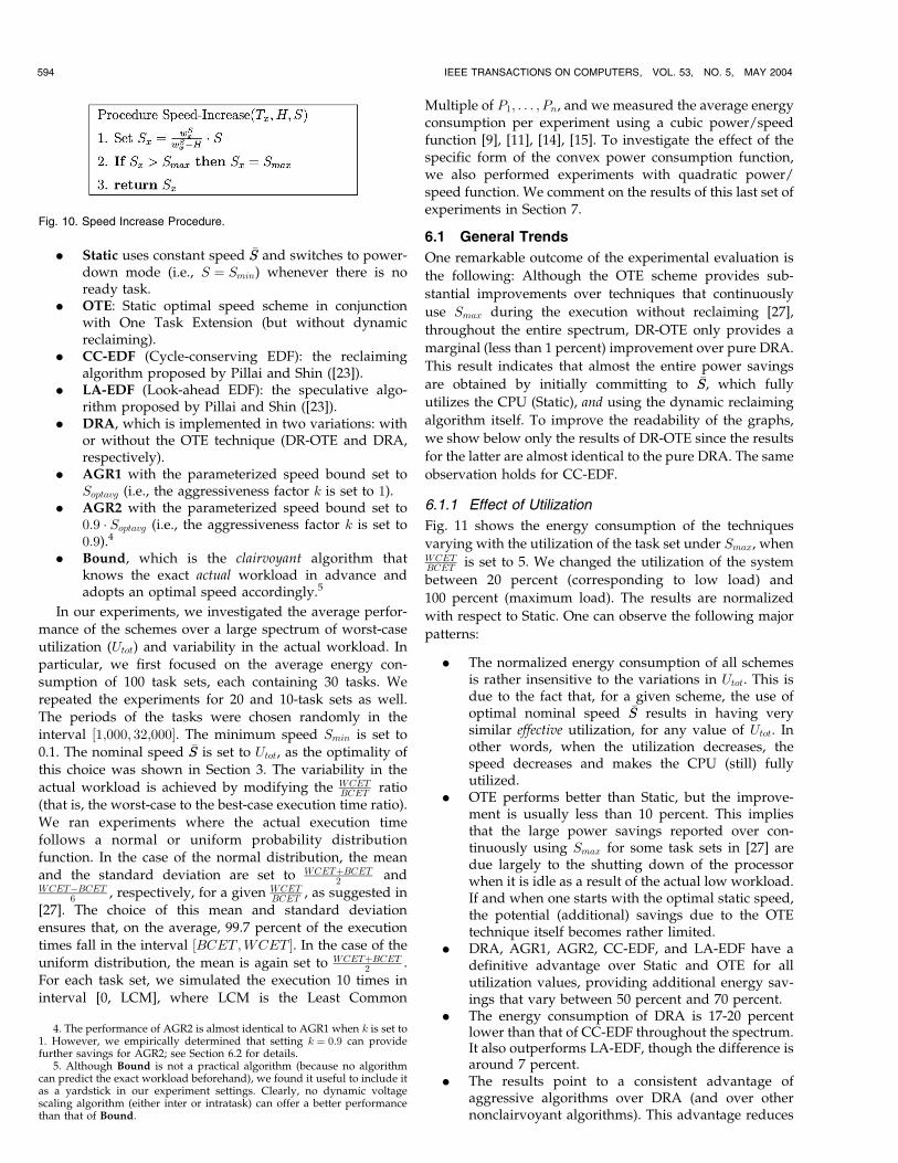
6.1.1 Effect of Utilization

Fig. 11 shows the energy consumption of the techniques

varying with the utilization of the task set under Smax, whenWCETBCET is set to 5. We changed the utilization of the system

between 20 percent (corresponding to low load) and

100 percent (maximum load). The results are normalized

with respect to Static. One can observe the following major

patterns:

. The normalized energy consumption of all schemesis rather insensitive to the variations in Utot. This isdue to the fact that, for a given scheme, the use ofoptimal nominal speed �SS results in having verysimilar effective utilization, for any value of Utot. Inother words, when the utilization decreases, thespeed decreases and makes the CPU (still) fullyutilized.

. OTE performs better than Static, but the improve-ment is usually less than 10 percent. This impliesthat the large power savings reported over con-tinuously using Smax for some task sets in [27] aredue largely to the shutting down of the processorwhen it is idle as a result of the actual low workload.If and when one starts with the optimal static speed,the potential (additional) savings due to the OTEtechnique itself becomes rather limited.

. DRA, AGR1, AGR2, CC-EDF, and LA-EDF have adefinitive advantage over Static and OTE for allutilization values, providing additional energy sav-ings that vary between 50 percent and 70 percent.

. The energy consumption of DRA is 17-20 percentlower than that of CC-EDF throughout the spectrum.It also outperforms LA-EDF, though the difference isaround 7 percent.

. The results point to a consistent advantage ofaggressive algorithms over DRA (and over othernonclairvoyant algorithms). This advantage reduces


Fig. 10. Speed Increase Procedure.

4. The performance of AGR2 is almost identical to AGR1 when k is set to1. However, we empirically determined that setting k ¼ 0:9 can providefurther savings for AGR2; see Section 6.2 for details.

5. Although Bound is not a practical algorithm (because no algorithmcan predict the exact workload beforehand), we found it useful to include itas a yardstick in our experiment settings. Clearly, no dynamic voltagescaling algorithm (either inter or intratask) can offer a better performancethan that of Bound.

as the utilization approaches 100 percent; at highutilization values, all tasks assume a nominal(default) speed close to Smax ¼ 1:0 and aggressivespeed reduction is not always possible because ofthe maximum speed constraint. It is also interestingto observe the near-optimal performance of AGR1and AGR2, especially in utilization values notexceeding 80 percent: The clairvoyant algorithmcould provide only 10 percent improvement overaggressive algorithms in that part of the spectrum.

. AGR2 performs slightly better than AGR1; wepresent a detailed performance comparison of bothalgorithms in Section 6.2.

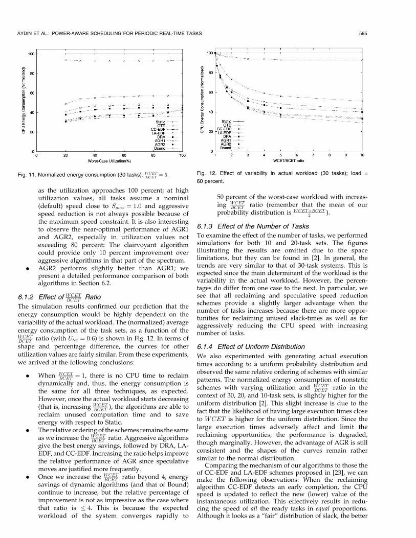
6.1.2 Effect of WCETBCET Ratio

The simulation results confirmed our prediction that theenergy consumption would be highly dependent on thevariability of the actual workload. The (normalized) averageenergy consumption of the task sets, as a function of theWCETBCET ratio (with Utot ¼ 0:6) is shown in Fig. 12. In terms ofshape and percentage difference, the curves for otherutilization values are fairly similar. From these experiments,we arrived at the following conclusions:

. When WCETBCET ¼ 1, there is no CPU time to reclaim

dynamically and, thus, the energy consumption isthe same for all three techniques, as expected.However, once the actual workload starts decreasing(that is, increasing WCET

BCET ), the algorithms are able toreclaim unused computation time and to saveenergy with respect to Static.

. The relative ordering of the schemes remains the sameas we increase the WCET

BCET ratio. Aggressive algorithmsgive the best energy savings, followed by DRA, LA-EDF, and CC-EDF. Increasing the ratio helps improvethe relative performance of AGR since speculativemoves are justified more frequently.

. Once we increase the WCETBCET ratio beyond 4, energy

savings of dynamic algorithms (and that of Bound)continue to increase, but the relative percentage ofimprovement is not as impressive as the case wherethat ratio is � 4. This is because the expectedworkload of the system converges rapidly to

50 percent of the worst-case workload with increas-ing WCET

BCET ratio (remember that the mean of ourprobability distribution is WCETþBCET

2 ).

6.1.3 Effect of the Number of Tasks

To examine the effect of the number of tasks, we performedsimulations for both 10 and 20-task sets. The figuresillustrating the results are omitted due to the spacelimitations, but they can be found in [2]. In general, thetrends are very similar to that of 30-task systems. This isexpected since the main determinant of the workload is thevariability in the actual workload. However, the percen-tages do differ from one case to the next. In particular, wesee that all reclaiming and speculative speed reductionschemes provide a slightly larger advantage when thenumber of tasks increases because there are more oppor-tunities for reclaiming unused slack-times as well as foraggressively reducing the CPU speed with increasingnumber of tasks.

6.1.4 Effect of Uniform Distribution

We also experimented with generating actual executiontimes according to a uniform probability distribution andobserved the same relative ordering of schemes with similarpatterns. The normalized energy consumption of nonstaticschemes with varying utilization and WCET

BCET ratio in thecontext of 30, 20, and 10-task sets, is slightly higher for theuniform distribution [2]. This slight increase is due to thefact that the likelihood of having large execution times closeto WCET is higher for the uniform distribution. Since thelarge execution times adversely affect and limit thereclaiming opportunities, the performance is degraded,though marginally. However, the advantage of AGR is stillconsistent and the shapes of the curves remain rathersimilar to the normal distribution.

Comparing the mechanism of our algorithms to those theof CC-EDF and LA-EDF schemes proposed in [23], we canmake the following observations: When the reclaimingalgorithm CC-EDF detects an early completion, the CPUspeed is updated to reflect the new (lower) value of theinstantaneous utilization. This effectively results in redu-cing the speed of all the ready tasks in equal proportions.Although it looks as a “fair” distribution of slack, the better


Fig. 11. Normalized energy consumption (30 tasks). WCETBCET ¼ 5. Fig. 12. Effect of variability in actual workload (30 tasks); load =

60 percent.

performance offered by DRA hints at the fact that a greedyapproach is more effective when the actual workloaddeviates from the worst-case scenario. Essentially, DRAassigns the entire slack to the first low-priority task that isabout to run. This greedy strategy pays off in the long runsince, in many cases, this “lucky” task completes early aswell and subsequent tasks are able to use its slack. Thus, ingeneral, we can say that overprovisioning while distribut-ing the available slack during the reclaiming phase hindersenergy savings.

The same observation holds for LA-EDF. This algorithmuses the CPU time borrowed from future task instances tospeculatively lower the instantaneous utilization overmultiple tasks, thereby limiting the speed reduction thatcan be applied to the first task to run. In contrast, ouraggressive algorithms “steal” CPU time from other readytasks to the exclusive benefit of the dispatched task. Theexperiments show that the performance is best when theaggressive slow-down is limited by the speed that would beoptimal under the expected workload of the task set. Beforeconcluding this section, we note that a recent study [12]provided an independent experimental evaluation of theseschemes, confirming the success of AGR and DRA whencompared to other existing techniques.

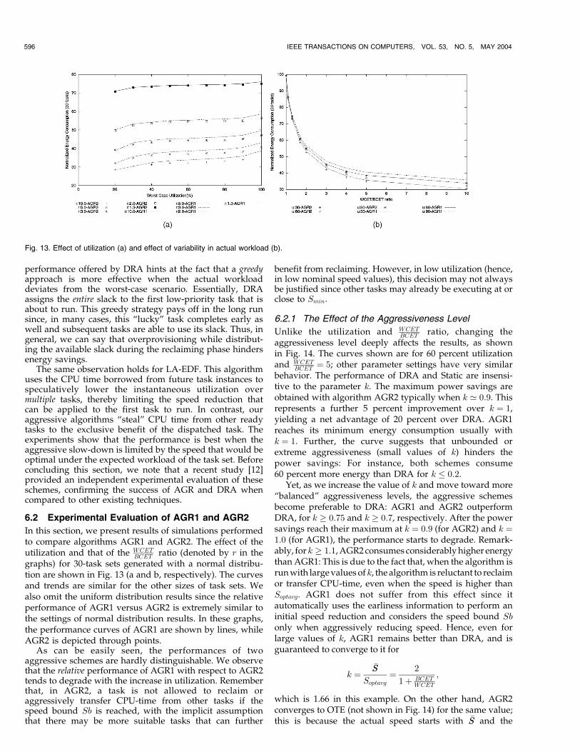
6.2 Experimental Evaluation of AGR1 and AGR2

In this section, we present results of simulations performedto compare algorithms AGR1 and AGR2. The effect of theutilization and that of the WCET

BCET ratio (denoted by r in thegraphs) for 30-task sets generated with a normal distribu-tion are shown in Fig. 13 (a and b, respectively). The curvesand trends are similar for the other sizes of task sets. Wealso omit the uniform distribution results since the relativeperformance of AGR1 versus AGR2 is extremely similar tothe settings of normal distribution results. In these graphs,the performance curves of AGR1 are shown by lines, whileAGR2 is depicted through points.

As can be easily seen, the performances of twoaggressive schemes are hardly distinguishable. We observethat the relative performance of AGR1 with respect to AGR2tends to degrade with the increase in utilization. Rememberthat, in AGR2, a task is not allowed to reclaim oraggressively transfer CPU-time from other tasks if thespeed bound Sb is reached, with the implicit assumptionthat there may be more suitable tasks that can further

benefit from reclaiming. However, in low utilization (hence,in low nominal speed values), this decision may not alwaysbe justified since other tasks may already be executing at orclose to Smin.

6.2.1 The Effect of the Aggressiveness Level

Unlike the utilization and WCETBCET ratio, changing the

aggressiveness level deeply affects the results, as shownin Fig. 14. The curves shown are for 60 percent utilizationand WCET

BCET ¼ 5; other parameter settings have very similarbehavior. The performance of DRA and Static are insensi-tive to the parameter k. The maximum power savings areobtained with algorithm AGR2 typically when k ’ 0:9. Thisrepresents a further 5 percent improvement over k ¼ 1,yielding a net advantage of 20 percent over DRA. AGR1reaches its minimum energy consumption usually withk ¼ 1. Further, the curve suggests that unbounded orextreme aggressiveness (small values of k) hinders thepower savings: For instance, both schemes consume60 percent more energy than DRA for k � 0:2.

Yet, as we increase the value of k and move toward more“balanced” aggressiveness levels, the aggressive schemesbecome preferable to DRA: AGR1 and AGR2 outperformDRA, for k � 0:75 and k � 0:7, respectively. After the powersavings reach their maximum at k ¼ 0:9 (for AGR2) and k ¼1:0 (for AGR1), the performance starts to degrade. Remark-ably, fork � 1:1,AGR2consumes considerablyhigher energythan AGR1: This is due to the fact that, when the algorithm isrunwith largevaluesofk, thealgorithm is reluctant to reclaimor transfer CPU-time, even when the speed is higher thanSoptavg. AGR1 does not suffer from this effect since itautomatically uses the earliness information to perform aninitial speed reduction and considers the speed bound Sbonly when aggressively reducing speed. Hence, even forlarge values of k, AGR1 remains better than DRA, and isguaranteed to converge to it for

k ¼�SS

Soptavg¼ 2

1þ BCETWCET

;

which is 1.66 in this example. On the other hand, AGR2converges to OTE (not shown in Fig. 14) for the same value;this is because the actual speed starts with �SS and the


Fig. 13. Effect of utilization (a) and effect of variability in actual workload (b).

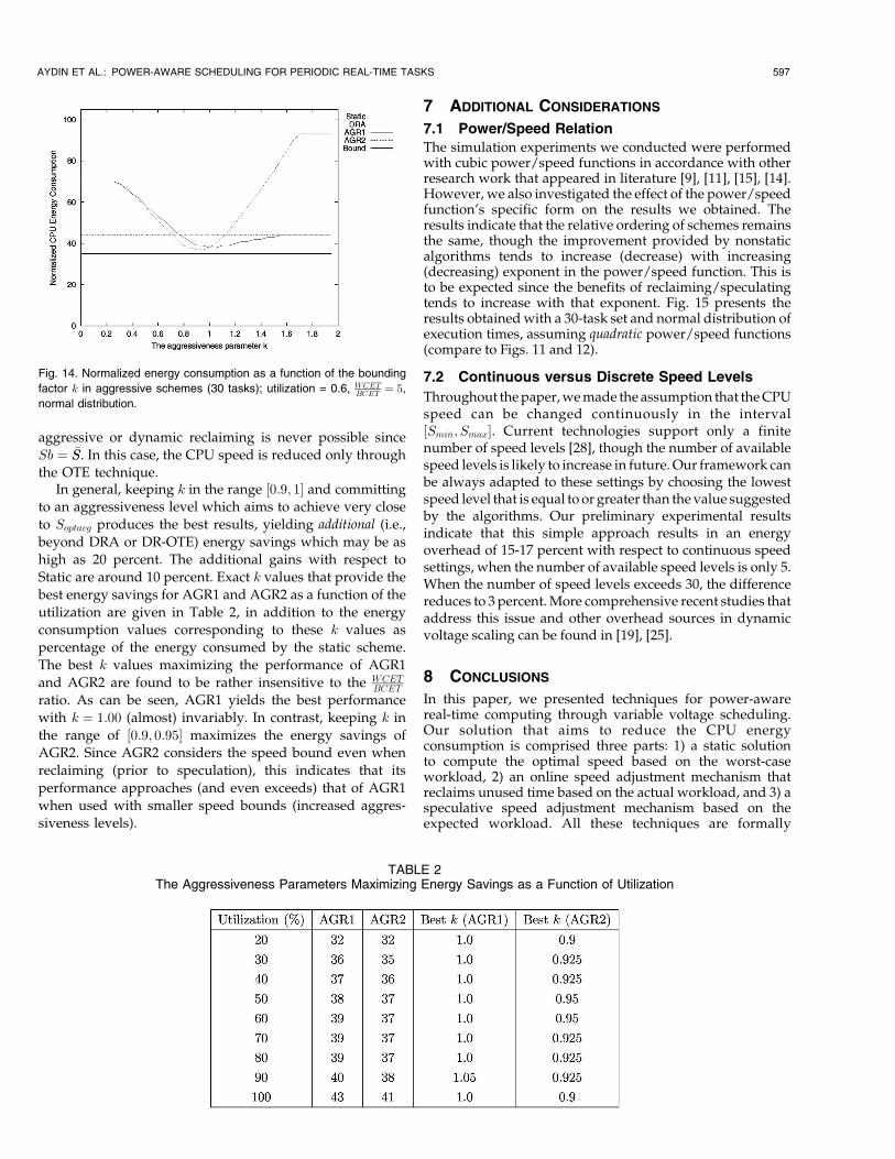
aggressive or dynamic reclaiming is never possible since

Sb ¼ �SS. In this case, the CPU speed is reduced only through

the OTE technique.In general, keeping k in the range ½0:9; 1� and committing

to an aggressiveness level which aims to achieve very close

to Soptavg produces the best results, yielding additional (i.e.,

beyond DRA or DR-OTE) energy savings which may be as

high as 20 percent. The additional gains with respect to

Static are around 10 percent. Exact k values that provide the

best energy savings for AGR1 and AGR2 as a function of the

utilization are given in Table 2, in addition to the energy

consumption values corresponding to these k values as

percentage of the energy consumed by the static scheme.

The best k values maximizing the performance of AGR1

and AGR2 are found to be rather insensitive to the WCETBCET

ratio. As can be seen, AGR1 yields the best performance

with k ¼ 1:00 (almost) invariably. In contrast, keeping k in

the range of ½0:9; 0:95� maximizes the energy savings of

AGR2. Since AGR2 considers the speed bound even when

reclaiming (prior to speculation), this indicates that its

performance approaches (and even exceeds) that of AGR1

when used with smaller speed bounds (increased aggres-

siveness levels).

7 ADDITIONAL CONSIDERATIONS

7.1 Power/Speed Relation

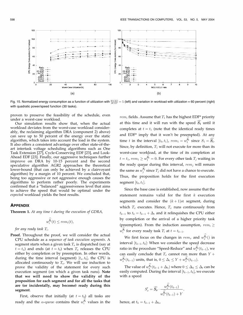
The simulation experiments we conducted were performedwith cubic power/speed functions in accordance with otherresearch work that appeared in literature [9], [11], [15], [14].However, we also investigated the effect of the power/speedfunction’s specific form on the results we obtained. Theresults indicate that the relative ordering of schemes remainsthe same, though the improvement provided by nonstaticalgorithms tends to increase (decrease) with increasing(decreasing) exponent in the power/speed function. This isto be expected since the benefits of reclaiming/speculatingtends to increase with that exponent. Fig. 15 presents theresults obtainedwith a 30-task set and normal distribution ofexecution times, assuming quadratic power/speed functions(compare to Figs. 11 and 12).

7.2 Continuous versus Discrete Speed Levels

Throughout thepaper,wemade the assumption that theCPUspeed can be changed continuously in the interval½Smin; Smax�. Current technologies support only a finitenumber of speed levels [28], though the number of availablespeed levels is likely to increase in future.Our framework canbe always adapted to these settings by choosing the lowestspeed level that is equal to or greater than the value suggestedby the algorithms. Our preliminary experimental resultsindicate that this simple approach results in an energyoverhead of 15-17 percent with respect to continuous speedsettings, when the number of available speed levels is only 5.When the number of speed levels exceeds 30, the differencereduces to 3 percent.More comprehensive recent studies thataddress this issue and other overhead sources in dynamicvoltage scaling can be found in [19], [25].

8 CONCLUSIONS

In this paper, we presented techniques for power-awarereal-time computing through variable voltage scheduling.Our solution that aims to reduce the CPU energyconsumption is comprised three parts: 1) a static solutionto compute the optimal speed based on the worst-caseworkload, 2) an online speed adjustment mechanism thatreclaims unused time based on the actual workload, and 3) aspeculative speed adjustment mechanism based on theexpected workload. All these techniques are formally


Fig. 14. Normalized energy consumption as a function of the bounding

factor k in aggressive schemes (30 tasks); utilization = 0.6, WCETBCET ¼ 5,

normal distribution.

TABLE 2The Aggressiveness Parameters Maximizing Energy Savings as a Function of Utilization

proven to preserve the feasibility of the schedule, evenunder a worst-case workload.

Our simulation results show that, when the actualworkload deviates from the worst-case workload consider-ably, the reclaiming algorithm DRA (component 2) above)can save up to 50 percent of the energy over the staticalgorithm, which takes into account the load in the system.It also offers a consistent advantage over other state-of-the-art intertask voltage scheduling algorithms such as OneTask Extension [27], Cycle-Conserving EDF [23], and Look-Ahead EDF [23]. Finally, our aggressive techniques furtherimprove on DRA by 10-15 percent and the secondspeculative algorithm AGR2 approaches the theoreticallower-bound (that can only be achieved by a clairvoyantalgorithm) by a margin of 10 percent. We concluded that,being too aggressive or not aggressive enough causes thealgorithms to perform rather poorly. The experimentsconfirmed that a “balanced” aggressiveness level that aimsto achieve the speed that would be optimal under theexpected workload yields the best results.

APPENDIX

Theorem 1. At any time t during the execution of GDRA,

wbSiSi

i ðtÞ � remiðtÞ;

for any ready task Ti.

Proof. Throughout the proof, we will consider the actualCPU schedule as a sequence of task execution segments. Asegment starts when a given task Ta is dispatched (say att ¼ ta) and ends (at t ¼ tb) when Ta releases the CPUeither by completion or by preemption. In other words,during the time interval (segment) ½ta; tb�, the CPU isallocated continuously to Ta. We will use induction toprove the validity of the statement for every suchexecution segment (on which a given task runs). Notethat we will need to show the validity of theproposition for each segment and for all the tasks thatare (or incidentally, may become) ready during thissegment.

First, observe that initially (at t ¼ t0) all tasks are

ready and the �-queue contains their wbSiSi

i values in the

remi fields. Assume that T1 has the highest EDF* priority

at this time and it will run with the speed cS1S1 until it

completes at t ¼ t1 (note that the identical ready times

and EDF* imply that it won’t be preempted). At any

time t in the interval ½t0; t1Þ, rem1 ¼ wbS1S1

1 since S1 ¼ cS1S1.

Since, by definition, T1 will not execute for more than its

worst-case workload, at the time of its completion at

t ¼ t1, rem1 � wbS1S1

1 ¼ 0. For every other task Tj waiting in

the ready queue during this interval, remj will remain

the same as wbSjSj

j since Tj did not have a chance to execute.

Thus, the proposition holds for the first execution

segment ½t0; t1�.

Since the base case is established, now assume that the

statement remains valid for the first k execution

segments and consider the ðkþ 1Þst segment, during

which Tx executes. Hence, Tx runs continuously from

tk�1 to tk ¼ tk�1 þ�t and it relinquishes the CPU either

by completion or the arrival of a higher priority task

(preemption). From the induction assumption, remi �wbSiSi

i for every ready task Ti at t ¼ tk�1.

We first focus on the changes in remx and wbSxSxx ðÞ in

interval ½tk�1; tk�: When we consider the speed decrease

ratio in the procedure “Speed-Reduce” and wbSxSxx ðtk�1Þ, we

can easily conclude that Tx cannot run more than Y þwbSxSxx ðtk�1Þ units, that is, 0 � �t � Y þ w

bSxSxx ðtk�1Þ.

The value of wbSxSxx ðtk�1 þ�hÞwhere 0 � �h � �t can be

easily computed. During the interval ½tk�1; tk�, we executewith a speed

S0x ¼ cSxSx �

wbSxSxx ðtk�1Þ

wbSxSxx ðtk�1Þ þ Y

;

hence, at th ¼ tk�1 þ�h,


Fig. 15. Normalized energy consumption as a function of utilization with WCETBCET ¼ 5 (left) and variation in workload with utilization = 60 percent (right)

with quadratic power/speed function (30 tasks).

wbSxSxx ðthÞ ¼ w

bSxSxx ðtk�1Þ �

S0xcSxSx

�h

¼ wbSxSxx ðtk�1Þ 1� �h

Y þ wbSxSxx ðtk�1Þ

24

35 � 0;

for the preemption case, or wbSxSxx ðth ¼ tkÞ ¼ 0, for the

completion case.

What is the value of remxðtk�1 þ�hÞ? Let us

define by �hðt; xÞ the sum of all remi values in the

�-queue at time t, such that Ti has strictly higher

EDF* priority than Tx. Observe that, by definition,

�xðtÞ ¼ �hðt; xÞ þ remxðtÞ � wbSxSxx ðtÞ. Hence:

remxðtk�1Þ ¼ �xðtk�1Þ þ wbSxSxx ðtk�1Þ � �hðtk�1; xÞ: ð1Þ

As time elapses, we consume from the �-queue,starting from the head. We distinguish two cases:

. If �h � �hðtk�1; xÞ, we will only consume theslack of “higher” priority tasks in the �-queue andremx will remain intact. Hence, using also theinduction assumption, we can obtain:

remxðtk�1 þ�hÞ ¼ remxðtk�1Þ � wbSxSxx ðtk�1Þ

� wbSxSxx ðtk�1 þ�hÞ4

for this special case.. If �hðtk�1; xÞ < �h � �t � Y þ w

bSxSxðtk�1Þx , we will

start decreasing remx value only att ¼ tk�1 þ �hðtk�1; xÞ. At t ¼ tk�1 þ�h,

remxðtk�1 þ�hÞ ¼ remxðtk�1Þ � ð�h � �hðtk�1; xÞÞ

and, using (1), we get:

remxðtk�1 þ�hÞ ¼ �xðtk�1Þ þ wbSxSxx ðtk�1Þ ��h

� Y þ wbSxSxx ðtk�1Þ ��h

¼ ðY þ wbSxSxx ðtk�1ÞÞ 1� �h


24

35

� wbSxSxx ðtk�1Þ 1� �h


24

35 ¼ w

bSxSxx ðtk�1 þ�hÞ:

Thus, for task Tx, we have remxðtk�1 þ�hÞ �wbSxSxx ðtk�1 þ�hÞ � 0 for 0 � �h � �t � Y þ w

bSxSxx ðtk�1Þ. A

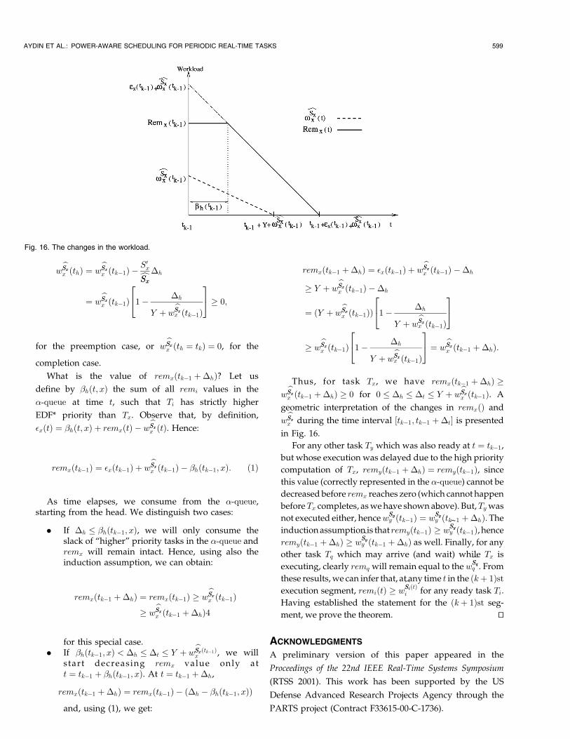
geometric interpretation of the changes in remxðÞ and

wbSxSxx during the time interval ½tk�1; tk�1 þ�t� is presented

in Fig. 16.

For any other task Ty which was also ready at t ¼ tk�1,

but whose execution was delayed due to the high priority

computation of Tx, remyðtk�1 þ�hÞ ¼ remyðtk�1Þ, sincethis value (correctly represented in the �-queue) cannot be

decreased before remx reaches zero (which cannot happen

beforeTx completes, aswehave shownabove). But,Ty was

not executed either, hencewbSySyy ðtk�1Þ ¼ w

bSySyy ðtk�1 þ�hÞ. The

inductionassumption is that remyðtk�1Þ � wbSySyy ðtk�1Þ, hence

remyðtk�1 þ�hÞ � wbSySyy ðtk�1 þ�hÞ as well. Finally, for any

other task Tq which may arrive (and wait) while Tx is

executing, clearly remq will remain equal to the wbSqSqq . From

these results,we can infer that, at any time t in the ðkþ 1Þstexecution segment, remiðtÞ � w

bSiSiðtÞi for any ready task Ti.

Having established the statement for the ðkþ 1Þst seg-

ment, we prove the theorem. tu

ACKNOWLEDGMENTS

A preliminary version of this paper appeared in the

Proceedings of the 22nd IEEE Real-Time Systems Symposium

(RTSS 2001). This work has been supported by the US

Defense Advanced Research Projects Agency through the

PARTS project (Contract F33615-00-C-1736).


Fig. 16. The changes in the workload.

REFERENCES

[1] H. Aydin, R. Melhem, D. Mosse, and P.M. Alvarez, “OptimalReward-Based Scheduling for Periodic Real-Time Tasks,” IEEETrans. Computers, vol. 50, no. 2, pp. 111-130, Feb. 2001.

[2] H. Aydin, “Enhancing Performance and Fault Tolerance inReward-Based Scheduling,” PhD dissertation, Univ. of Pittsburgh,Aug. 2001, http://www.cs.gmu.edu/~aydin/dissertation.

[3] J.K. Dey, J. Kurose, and D. Towsley, “On-Line Scheduling Policiesfor a Class of IRIS (Increasing Reward with Increasing Service)Real-Time Tasks,” IEEE Trans. Computers, vol. 45, no. 7, pp. 802-813, July 1996.

[4] R. Ernst and W. Ye, “Embedded Program Timing Analysis Basedon Path Clustering and Architecture Classification,” Proc. Int’lConf. Computer-Aided Design (ICCAD ’97) pp. 598-604, 1997.

[5] F. Gruian, “Hard Real-Time Scheduling for Low-Energy UsingStochastic Data and DVS Processors,” Proc. Int’l Symp. Low PowerElectronics and Design 2001, Aug. 2001.

[6] V. Gutnik and A. Chandrakasan, “An Efficient Controller forVariable Supply Voltage Low Power Processing,” Proc. Symp.VLSI Circuits, pp. 158-159, 1996.

[7] I. Hong, D. Kirovski, G. Qu, M. Potkonjak, and M. Srivastava,“Power Optimization of Variable Voltage Core-Based Systems,”Proc. 35th Design Automation Conf. (DAC ’98), 1998.

[8] I. Hong, M. Potkonjak, and M.B. Srivastava, “On-Line Schedulingof Hard Real-Time Tasks on Variable Voltage Processor,” Proc.Computer-Aided Design (ICCAD ’98), pp. 653-656, 1998.

[9] I. Hong, G. Qu, M. Potkonjak, and M. Srivastava, “SynthesisTechniques for Low-Power Hard Real-Time Systems on VariableVoltage Processors,” Proc. 19th IEEE Real-Time Systems Symp.(RTSS ’98), Dec. 1998.

[10] Intel, Microsoft, and Toshiba, “Advanced Configuration andPower Management Interface (ACPI) Specification,” 1999,www.intel.com/ial/WfM/design/pmdt/acpidesc.htm.

[11] R. Jejurikar and R. Gupta, “Energy Aware Task Scheduling withTask Synchronization for Embedded Real Time Systems,” Proc.Int’l Conf. Compilers, Architecture and Synthesis for EmbeddedSystems, Oct. 2002.

[12] W. Kim, D. Shin, H.S. Yun, J. Kim, and S.L. Min, “PerformanceComparison of Dynamic Voltage Scaling Algorithms for HardReal-Time Systems,” Proc. Eighth Real-Time Technology andApplications Symp., 2002.

[13] C.M. Krishna and Y.H. Lee, “Voltage Clock Scaling AdaptiveScheduling Techniques for Low Power in Hard Real-TimeSystems,” Proc. Sixth IEEE Real-Time Technology and ApplicationsSymposium (RTAS ’00), May 2000.

[14] P. Kumar and M. Srivastava, “Power-Aware Multimedia SystemsUsing Run-Time Prediction,” Proc. 13th Int’l Conf. ComputerDesign, Jan. 2001.

[15] T. Li and C. Ding, “Instruction Balance and Its Relation toProgram Energy Consumption,” Proc. Int’l Workshop Languages andCompilers for Parallel Computing, Aug. 2001.

[16] C.L. Liu and J.W. Layland, “Scheduling Algorithms for Multi-programming in Hard Real-Time Environment,” J. ACM, vol. 20,no. 1, pp. 46-61, 1973.

[17] J.R. Lorch, “A Complete Picture of the Energy Consumption of aPortable Computer,” master’s thesis, Univ. of California, Berkeley,Dec. 1995.

[18] J.R. Lorch and A.J. Smith, “Improving Dynamic Voltage ScalingAlgorithms with PACE,” Proc. ACM SIGMETRICS 2001 Conf., June2001.

[19] B. Mochocki, X. Hu, and G. Quan, “A Realistic Variable VoltageScheduling Model for Real-Time Applications,” Proc. Int’l Conf.Computer Aided Design (ICCAD 2002), 2002.

[20] D. Mosse, H. Aydin, B. Childers, and R. Melhem, “Compiler-Assisted Dynamic Power-Aware Scheduling for Real-Time Ap-plications,” Proc. Workshop Compilers and Operating Systems forLow-Power (COLP ’00), Oct. 2000.

[21] W. Namgoang, M. Yu, and T. Meg, “A High Efficiency Variable-Voltage CMOS Dynamic DC-DC Switching Regulator,” Proc. IEEEInt’l Solid-State Circuits Conf., pp. 380-391, 1997.

[22] T. Pering and R. Brodersen, “Energy Efficient Voltage Schedulingfor Real-Time Systems,” Proc. Fourth Real-Time Technology andApplications Symp., WIP Session, 1998.

[23] P. Pillai and K.G. Shin, “Real-Time Dynamic Voltage Scaling forLow Power Embedded Operating Systems,” Proc. 18th Symp.Operating System Principles, Oct. 2001.

[24] J. Pouwelse, K. Langendoen, and H. Sips, “Dynamic VoltageScaling on a Low-Power Microprocessor,” Proc. Seventh Int’l Conf.Mobile Computing and Networking (MOBICOM), July 2001.

[25] S. Saewong and R. Rajkumar, “Practical Voltage-Scaling for Fixed-Priority Real-Time Systems,” Proc. Ninth IEEE Real-Time andEmbedded Technology and Applications Symp. (RTAS ’03), May 2003.

[26] D. Shin, S. Lee, and J. Kim, “Intra-Task Voltage Scheduling forLow-Energy Hard Real-Time Applications,” IEEE Design and Testof Computers, Mar. 2001.

[27] Y. Shin and K. Choi, “Power Conscious Fixed Priority Schedulingfor Hard Real-Time Systems,” Proc. 36th Design Automation Conf.(DAC ’99), pp. 134-139, 1999.

[28] http://www.transmeta.com, 2000.[29] M. Weiser, B. Welch, A. Demers, and S. Shenker, “Scheduling for

Reduced CPU Energy,” Proc. First Symp. Operating Systems Designand Implementation, 1994.

[30] F. Yao, A. Demers, and S. Shenker, “A Scheduling Model forReduced CPU Energy,” IEEE Ann. Foundations of Computer Science,pp. 374-382, 1995.

[31] H. Zeng, X. Fan, C. Ellis, A. Lebeck, and A. Vahdat, “ECOSystem:Managing Energy as a First Class Operating System Resource,”Proc. Int’l Conf. Architectural Support for Programming Languages andOperating Systems (ASPLOS 2002), Oct. 2002.

Hakan Aydin received the BS and MS degreesin control and computer engineering fromIstanbul Technical University in 1991 and 1994,respectively. In 1996, he joined the University ofPittsburgh Computer Science Departmentwhere he received the PhD degree in 2001. Heis currently an assistant professor at GeorgeMason University, Computer Science Depart-ment. His research interests include real-timesystems, low-power computing and fault toler-

ance. He is a member of the IEEE Computer Society.

Rami Melhem received the BE degree inelectrical engineering from Cairo University in1976, the MA degree in mathematics and theMS degree in computer science from theUniversity of Pittsburgh in 1981, and the PhDdegree in computer science from the Universityof Pittsburgh in 1983. He was an assistantprofessor at Purdue University prior to joiningthe faculty of the University of Pittsburgh in1986, where he is currently a professor of

computer science and electrical engineering and the chair of theComputer Science Department. His research interests include real-timeand fault-tolerant systems, optical interconnection networks, highperformance computing, and parallel computer architectures. He is afellow of the IEEE and a member of the ACM.

Daniel Mosse received the BS degree inmathematics from the University of Brasilia in1986 and the MS and PhD. degrees in computerscience from the University of Maryland in 1990and 1993, respectively. He joined the faculty ofthe University of Pittsburgh in 1992, where he iscurrently an associate professor. His researchinterests include fault-tolerant and real-timesystems, as well as networking. His maininterest is power-aware computing and security.

He is a member of the IEEE Computer Society and of the ACM.

Pedro Mejıa-Alvarez received the BS degree incomputer systems engineering from ITESM,Queretaro, Mexico, in 1985, and the PhD degreein informatics from the Universidad Politecnicade Madrid, Spain, in 1995. He has been anasisistant professor in Seccion de ComputacionCINVESTAV-IPN Mexico since 1997. He is afellow of the National System of Researchers ofMexico (SNI). His main research interests arereal-time systems scheduling, low-power com-

puting, adaptive fault tolerance, and software engineering. He is amember of the IEEE Computer Society.


Power-aware scheduling for periodic real-time tasks ...people.cs.pitt.edu/~melhem/vita/doc/01275298.pdfPower-Aware Scheduling for Periodic Real-Time Tasks Hakan Aydin, Member, IEEE

Documents