Powell–Sabin splines with boundary conditions for polygonal and non-polygonal domains

Powell-Sabin splines with boundary

conditions for polygonal and

non-polygonal domains

Hendrik Speleers

Paul Dierckx

Stefan Vandewalle

Report TW452, March 2006

Katholieke Universiteit LeuvenDepartment of Computer Science

Celestijnenlaan 200A – B-3001 Heverlee (Belgium)

Powell-Sabin splines with boundary

conditions for polygonal and

non-polygonal domains

Hendrik Speleers

Paul Dierckx

Stefan Vandewalle

Report TW452, March 2006

Department of Computer Science, K.U.Leuven

Abstract

Powell-Sabin splines are piecewise quadratic polynomials with aglobal C1-continuity, defined on conforming triangulations. Impos-ing a boundary condition on such a spline leads to a set of constraintson the spline coefficients. First we discuss boundary conditions de-fined on a polygonal domain, before we treat boundary conditionson a general curved domain boundary. We consider Dirichlet andNeumann conditions, and we show that a particular choice of thePS-triangles at the boundary can greatly simplify the correspondingconstraints. Finally, we consider an application where the techniquesdevelopped in this paper are used: the numerical solution of a partialdifferential equation by the Galerkin and collocation method.

Keywords : Powell-Sabin splines, boundary conditionsAMS(MOS) Classification : Primary : 41A29, Secondary : 65N30, 41A15

Powell-Sabin splines with boundary conditions for

polygonal and non-polygonal domains

Hendrik Speleers, Paul Dierckx and Stefan Vandewalle

Department of Computer Science, Katholieke Universiteit Leuven

Celestijnenlaan 200A, B-3001 Leuven, Belgium

Abstract

Powell-Sabin splines are piecewise quadratic polynomials with a global C1-continuity, defined

on conforming triangulations. Imposing a boundary condition on such a spline leads to a set

of constraints on the spline coefficients. First we discuss boundary conditions defined on a

polygonal domain, before we treat boundary conditions on a general curved domain boundary.

We consider Dirichlet and Neumann conditions, and we show that a particular choice of the

PS-triangles at the boundary can greatly simplify the corresponding constraints. Finally, we

consider an application where the techniques developped in this paper are used: the numerical

solution of a partial differential equation by the Galerkin and collocation method.

Keywords: Powell-Sabin splines, boundary conditions

AMS classification: 41A29, 65N30, 41A15, 65D07

1 Introduction

In computer-aided geometric design and scientific computing it is often important that a function orsurface preserves certain geometric properties, e.g. boundary conditions. Chui and Schumaker [3]were the first to investigate spaces of piecewise polynomial surfaces with boundary conditions. Theyconsidered splines on a rectangle partitioned into subrectangles, with vanishing normal derivativeson the boundary. In [3], the dimension of these spaces was computed and an appropriate localbasis was constructed. This study was continued in [4, 5] for spaces of boundary constrainedpiecewise polynomials on type-1 and type-2 triangulations. Such triangulations are constructed bysubdividing rectangular partitions of a rectangular domain by using the diagonals.

Shi et al. [15] studied the dimension and suggested a basis for the so-called Powell-Sabin (PS-)spline space subject to homogeneous Dirichlet and Neumann boundary conditions. Powell-Sabinsplines are piecewise quadratic polynomials with a global C1-continuity, defined on conformingtriangulations. Willemans and Dierckx used in [19] constrained Powell-Sabin splines for smoothingscattered noisy measurement data. Speleers et al. [17] treated Dirichlet boundary conditions, i.e.u(x, y) = f(x, y), and Neumann boundary conditions, i.e. ∂

∂nu(x, y) = g(x, y), with arbitraryboundary functions f(x, y) and g(x, y), imposed on Powell Sabin splines in the context of a finiteelement method. The set of corresponding constraints on the PS-spline coefficients are very simpleby a particular choice of the basis functions at the boundary.

Another technique to deal with homogeneous Dirichlet conditions consists of multiplying the basisfunctions with a positive weight function that vanishes on the boundary of the domain. This ideabecame successful in connection with the R-function method of Rvachev [13]. It is very effective incombination with the classical tensor-product splines [14, 10]: a homogeneous boundary condition

1

2 POWELL-SABIN SPLINES 2

defined on an arbitrary curved boundary can be exactly imposed without loss of the approximationpower of the splines.

In this paper, we discuss a new approach for the treatment of Dirichlet and Neumann conditionson (a part of) the boundary with Powell-Sabin splines. Instead of choosing the basis functions atthe boundary differently for each type of condition, as in [17], we now derive an approach thatallows a uniform treatment for all cases. It results in a basis that is more stable, and that can beconstructed in advance, irrespective of the particular application. We also treat the situation wherethe boundary conditions are no longer defined on the polygonal boundary of the triangulation. Thiscase will enable an efficient and accurate boundary condition representation on general curvedboundaries.

The paper is organized as follows. Section 2 reviews the definition of the Powell-Sabin spline space,and recalls the construction of a normalized B-spline basis. In section 3 we discuss some generalcharacteristics of the Powell-Sabin spline at the boundary. Section 4 addresses the treatment ofdifferent boundary conditions defined on the boundary of the triangulation. In section 5 boundaryconditions on non-polygonal domains are considered. In each of those cases, we show that aparticular choice of the Powell-Sabin basis functions associated with the boundary vertices cangreatly simplify the boundary constraints. We illustrate our treatment of the boundary conditionsusing the Poisson equation. Finally, in section 7 we end with some concluding remarks.

2 Powell-Sabin splines

2.1 The space of Powell-Sabin splines

Consider a simply connected subset Ω ∈ R2 with polygonal boundary ∂Ω. Assume a conforming

triangulation ∆ of Ω is given, consisting of t triangles ρj , j = 1, . . . , t, and having n vertices Vk,k = 1, . . . , n. A triangulation is conforming if no triangle contains a vertex different from its ownthree vertices.

The Powell-Sabin (PS-)refinement ∆∗ of ∆ partitions each triangle ρj into six smaller triangleswith a common vertex Zj . This partition is defined algorithmically as follows:

1. Choose an interior point Zj in each triangle ρj . If two triangles ρi and ρj have a commonedge, then the line joining Zi and Zj should intersect the common edge at some point Rij .

2. Join each point Zj to the vertices of ρj .

3. For each edge of the triangle ρj

(a) which is common to a triangle ρi: join Zj to Rij ;

(b) which belongs to the boundary ∂Ω: join Zj to an arbitrary point R on that edge.

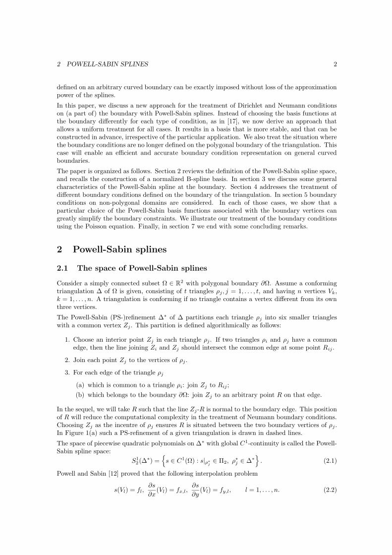
In the sequel, we will take R such that the line Zj-R is normal to the boundary edge. This positionof R will reduce the computational complexity in the treatment of Neumann boundary conditions.Choosing Zj as the incentre of ρj ensures R is situated between the two boundary vertices of ρj .In Figure 1(a) such a PS-refinement of a given triangulation is drawn in dashed lines.

The space of piecewise quadratic polynomials on ∆∗ with global C1-continuity is called the Powell-Sabin spline space:

S12(∆∗) =

s ∈ C1(Ω) : s|ρ∗

j∈ Π2, ρ∗j ∈ ∆∗

. (2.1)

Powell and Sabin [12] proved that the following interpolation problem

s(Vl) = fl,∂s

∂x(Vl) = fx,l,

∂s

∂y(Vl) = fy,l, l = 1, . . . , n. (2.2)

2 POWELL-SABIN SPLINES 3

(a) (b)

Figure 1: (a) A PS-refinement ∆∗ (dashed lines) of a given triangulation ∆ (solid lines); (b) thePS-points (bullets) and a set of suitable PS-triangles (shaded).

has a unique solution s(x, y) ∈ S12(∆∗) for any given set of n (fl, fx,l, fy,l)-values. It follows that

the dimension of the Powell-Sabin spline space S12(∆∗) is equal to 3n.

2.2 A normalized B-spline representation

Dierckx et al. [9] considered a suitable representation for Powell-Sabin splines. With each vertex Vi

three linearly independent triplets (αi,j , βi,j , γi,j), j = 1, 2, 3 are associated. The B-spline Bji (x, y)

can be found as the unique solution of interpolation problem (2.2) with all (fl, fx,l, fy,l) = (0, 0, 0)except for l = i, where (fi, fx,i, fy,i) = (αi,j , βi,j , γi,j) 6= (0, 0, 0). It is easy to see that this B-spline

has a local support: Bji (x, y) vanishes outside the so-called molecule Mi of Vi, meaning the union

of all triangles containing Vi. Every Powell-Sabin spline can then be represented as

s(x, y) =

n∑

i=1

3∑

j=1

ci,jBji (x, y). (2.3)

The basis forms a convex partition of unity on Ω if

Bji (x, y) ≥ 0, and

n∑

i=1

3∑

j=1

Bji (x, y) = 1, (2.4)

for all (x, y) ∈ Ω. This property, together with the local support of the Powell-Sabin B-splines, liesat the basis of their computational effectiveness in many application domains, see [9, 18, 11, 17].In [8] Dierckx has presented a geometrical way to derive and construct such a normalized basis:

1. For each vertex Vi ∈ ∆, identify the corresponding PS-points. These points are defined asthe midpoints of all edges in the PS-refinement ∆∗ containing Vi. The vertex Vi itself is alsoa PS-point. In Figure 1(b) the PS-points are indicated as bullets.

2. For each vertex Vi, find a triangle ti(Qi,1, Qi,2, Qi,3) containing all the PS-points of Vi. Thetriangles ti, i = 1, . . . , n are called PS-triangles. Note that the PS-triangles are not uniquely

3 THE CHARACTERIZATION OF A PS-SPLINE AT THE BOUNDARY 4

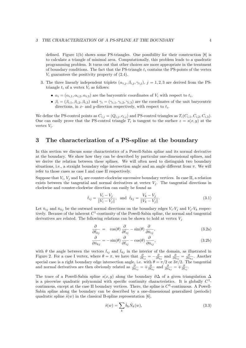
defined. Figure 1(b) shows some PS-triangles. One possibility for their construction [8] isto calculate a triangle of minimal area. Computationally, this problem leads to a quadraticprogramming problem. It turns out that other choices are more appropriate in the treatmentof boundary conditions. The fact that the PS-triangle ti contains the PS-points of the vertexVi guarantees the positivity property of (2.4).

3. The three linearly independent triplets (αi,j , βi,j , γi,j), j = 1, 2, 3 are derived from the PS-triangle ti of a vertex Vi as follows:

• αi = (αi,1, αi,2, αi,3) are the barycentric coordinates of Vi with respect to ti,

• βi = (βi,1, βi,2, βi,3) and γi = (γi,1, γi,2, γi,3) are the coordinates of the unit barycentricdirections, in x- and y-direction respectively, with respect to ti.

We define the PS-control points as Ci,j = (Qi,j , ci,j) and PS-control triangles as Ti(Ci,1, Ci,2, Ci,3).One can easily prove that the PS-control triangle Ti is tangent to the surface z = s(x, y) at thevertex Vi.

3 The characterization of a PS-spline at the boundary

In this section we discuss some characteristics of a Powell-Sabin spline and its normal derivativeat the boundary. We show how they can be described by particular one-dimensional splines, andwe derive the relation between these splines. We will often need to distinguish two boundarysituations, i.e., a straight boundary edge intersection angle and an angle different from π. We willrefer to those cases as case I and case II respectively.

Suppose that Vi, Vj and Vk are counter-clockwise successive boundary vertices. In case II, a relationexists between the tangential and normal derivatives at vertex Vj . The tangential directions inclockwise and counter-clockwise direction can easily be found as

tij =Vi − Vj

‖Vi − Vj‖, and tkj =

Vk − Vj

‖Vk − Vj‖. (3.1)

Let nij and nkj be the outward normal directions on the boundary edges Vi-Vj and Vj-Vk respec-tively. Because of the inherent C1-continuity of the Powell-Sabin spline, the normal and tangentialderivatives are related. The following relations can be shown to hold at vertex Vj

∂

∂tkj= cos(θ)

∂

∂tij− sin(θ)

∂

∂nij, (3.2a)

∂

∂nkj= − sin(θ)

∂

∂tij− cos(θ)

∂

∂nij, (3.2b)

with θ the angle between the vectors tij and tkj in the interior of the domain, as illustrated inFigure 2. For a case I vertex, where θ = π, we have that ∂

∂tij= − ∂

∂tkjand ∂

∂nij= ∂

∂nkj. Another

special case is a right boundary edge intersection angle, i.e. with θ = π/2 or 3π/2. The tangentialand normal derivatives are then obviously related as ∂

∂nij= ∓ ∂

∂tkjand ∂

∂nkj= ∓ ∂

∂tij.

The trace of a Powell-Sabin spline s(x, y) along the boundary ∂∆ of a given triangulation ∆is a piecewise quadratic polynomial with specific continuity characteristics. It is globally C1-continuous, except at the case II boundary vertices. There, the spline is C0-continuous. A Powell-Sabin spline along the boundary can be described by a one-dimensional generalized (periodic)quadratic spline s(w) in the classical B-spline representation [6],

s(w) =∑

k

bkNk(w), (3.3)


tij tkjnij nkj

θ

Vj

Vi Vk

Figure 2: Orientation of the tangential directions (tij and tkj), the normal directions (nij and nkj),and the edge intersection angle θ at the boundary vertex Vj .

with w the accumulated arc length in counter-clockwise direction. As in [17], we associate thespline knots tk with the positions of the vertices Vj and the points Rij . The lengths of the knotintervals preserve the distances between the points Rij and Vj . The notation and knot positions

are illustrated in Figure 3(b). The support of a quadratic B-spline Nk(w) is an interval spannedby four successive knots, starting with the knot tk.

The normal derivative of a Powell-Sabin spline along ∂∆ is a piecewise linear polynomial, which wewill represent by a one-dimensional generalized (periodic) linear spline s(w). As mentioned before,we chose the PS-refinement such that the interior line Z-Rij is normal to the boundary. Becauseof this choice, s(w) is linear on the edge Vi-Vj . This can be shown as follows. All points X on theline Z-Rij satisfy the equation

tij · (X − Rij) = 0. (3.4)

Consider a quadratic polynomial p(x, y) on triangle ρ(Vi, Rij , Z) and another quadratic polynomialq(x, y) on ρ(Rij , Vj , Z). The two patches are C1-continuous along the line Z-Rij if and only if

q(X) = p(X) + λ(

tij · (X − Rij))2

(3.5)

for some value of λ. Since the quadric z(X) =(

tij · (X − Rij))2

is a parabolic cylinder with itsaxis parallel to nij , it follows for all points in the combined triangle ρ(Vi, Vj , Z) that

∂ z

∂nij= 0, and, hence,

∂ q

∂nij=

∂ p

∂nij. (3.6)

Thus, the normal derivative of the Powell-Sabin spline is linear on the edge Vi-Vj . The 1D splines(w) may be discontinuous at the point Vj in case II, and is C0-continuous in case I. Figure 3(c)shows the knot positions and some basis functions used to represent s(w). Because of the linearityalong Vi-Vj , only knots at the boundary vertices are needed. The knots and coefficients of s(w)and s(w) are distinguished by tildes and hats respectively.

We now derive a relation between the coefficients of s(w) and s(w) at a case II boundary vertexVj . Let Rij = λijVi + λjiVj and Rjk = λjkVj + λkjVk with λij + λji = λjk + λkj = 1. Then

∂

∂tijs(Vj) = −s′(tj1−) =

2

λij

(bi2 − bij)

‖Vi − Vj‖, (3.7a)

∂

∂tkjs(Vj) = s′(tj1+) =

2

λkj

(bj1 − bij)

‖Vk − Vj‖. (3.7b)

The normal derivatives of the Powell-Sabin spline at the vertex Vj are equal to

∂

∂nijs(Vj) = s(tj1−) = bi2 , (3.8a)

∂

∂nkjs(Vj) = s(tj1+) = bj1 . (3.8b)


Vi Rij Vj Rjk Vk

Z

nij nkj

ViRij

Vj

Rjk

Vk

nij nkj

(a) Boundary triangles of a given triangulation with PS-refinement: case I (left) and case II (right)

ti1

ti2 tij tj1 tjk

tk1

tk2w

ti1

ti2 tijtj1

tj2 tjk

tk1

tk2w

(b) Knot positions and some 1D B-splines used to represent the value of a PS-spline along the boundary

ti1

ti2 tj1tk1

tk2w

ti1

ti2tj1

tj2tk1

tk2w

(c) Knot positions and some 1D B-splines used to represent the normal derivative of a PS-spline along theboundary

Figure 3: The knot positions and some 1D B-splines for the representation of (b) the value and(c) the normal derivative of a PS-spline along the boundary in case I and II.

Combining (3.7) and (3.8) with (3.2), we obtain a relation between the coefficients of the spliness(w) and s(w):

sin(θ) bi2 =2 cos(θ)

λij

(bi2 − bij)

‖Vi − Vj‖− 2

λkj

(bj1 − bij)

‖Vk − Vj‖, (3.9a)

sin(θ) bj1 =2 cos(θ)

λkj

(bj1 − bij)

‖Vk − Vj‖− 2

λij

(bi2 − bij)

‖Vi − Vj‖. (3.9b)

4 BOUNDARY CONDITIONS ON A POLYGONAL BOUNDARY 7

V1V2

V3

V4

V5

p1 p2 . . .

p15

p16

t2/t2t1/t1

t3 t4/t3 t5t7/t5t6/t4

t8t11

t9/t6

t10/t7

Figure 4: Example triangulation with knot positions for a Dirichlet (tk) and Neumann (tk) bound-ary condition. Two sample points pr are taken in each non-degenerated knot interval [tl, tl+1].

For a case I boundary vertex (θ = π) these relations reduce to

2

λkj

(bj1 − bij)

‖Vk − Vj‖+

2

λij

(bi2 − bij)

‖Vi − Vj‖= 0, (3.10)

which is just the C1-continuity relation between the spline coefficients of s(w) at Vj .

4 Boundary conditions on a polygonal boundary

We deal with the question of how to impose Dirichlet and Neumann boundary conditions on aPowell-Sabin spline. Physically, if that spline would represent, for example a temperature field,a Dirichlet condition corresponds to setting the value of the field variable, i.e. temperature. ANeumann condition specifies a flux condition on the boundary. We suppose that the boundarycondition is defined on a polygonal domain boundary, so we can follow the approach proposed in[17], consisting of two steps. In a first step the boundary function is projected into the Powell-Sabin spline space. Representing the PS-spline with a one-dimensional generalized (periodic)spline defined along the boundary, a discrete least squares method [7] can be used to find a goodapproximation. In a second step the constraints on the PS-spline coefficients are determined suchthat the trace of the PS-spline along the boundary equals the projected boundary function. Itturns out that a particular choice of the PS-triangles at the boundary can greatly simplify theseconstraints. We advocate an adaptation to the strategy in [17]: we will only use a single type ofPS-triangles at the boundary.

To illustrate the projection into the PS-space of the functions appearing in the right hand sides ofthese boundary conditions, we will refer each time to the triangulation in Figure 4. It consists of asingle case I boundary vertex (V2), and three case II boundary vertices (V1, V3, V4). The figure alsoshows corresponding knot positions of s(w) and of s(w), starting with t1 = t2 = t1 = t2 = 0. Thenumber of knots shown for each case is equal to the dimension of the corresponding 1D spline space.If we unfold the boundary of the triangulation to a straight line, we need to introduce some extraknots at both ends of the interval, e.g. t0, t12, and t13 to uniquely define s(w) =

∑11k=0 bkNk(w).

These knots are chosen such that t11− t0 = t12 = t13 equals the total boundary length, and b0 = b11


b1

b2

b3

b4

b5

b6

b7

b8

b9

b10

b11

Figure 5: Band structure of the overdetermined system∑

k bkNk(wr) = f(pr) for a Dirichletcondition on the boundary of the triangulation in Figure 4. Two interpolation points pr are chosenin each non-degenerated knot interval [tl, tl+1].

to retain the periodicity of the spline. Likewise, s(w) =∑7

k=1 bkNk(w) with t8 = t9 equal to theboundary length.

4.1 A Dirichlet boundary condition

A Dirichlet condition on a Powell-Sabin spline s(x, y) corresponds to the condition

s(x, y) = f(x, y), for (x, y) ∈ ∂Ω, (4.1)

for a given function f(x, y). A PS-spline cannot in general satisfy this condition exactly, unlessthe trace of f(x, y) along ∂Ω is a one-dimensional quadratic spline satisfying the characteristicsdiscussed in section 3. If this is not the case, we shall first project the function f into the appropriatespline space. Here, we suggest to use the approximation s(w) obtained by a discrete least squaresmethod. We take a number of evaluation points pr along the boundary (in the example of Figure4 two points in each knot interval), calculate the corresponding values wr for the accumulatedarc length, and determine the coefficients bk as the least squares solution of the overdeterminedsystem

∑

k bkNk(wr) = f(pr). Here, we can fully exploit the typical cyclic bandstructure as shownin Figure 5 for the triangulation in Figure 4.

Once the coefficients bk are known, one can proceed to derive the constraints on the PS-splinecoefficients ci,j in (2.3) such that the Powell-Sabin spline exactly matches s(w) at the boundary.The construction of those constraints is explained below. It is sufficient to impose the followingthree conditions for each vertex Vj (see [17])

s(Vj) = s(tj1),∂

∂tijs(Vj) = −s′(tj1−), and

∂

∂tkjs(Vj) = s′(tj1+). (4.2)

We choose the PS-triangle of Vj such that one side is parallel to the boundary edge Vi-Vj , andanother side of the PS-triangle is normal to that edge. Let τij and νij be such that

Qj,2 − Qj,1 = τij tij , and Qj,3 − Qj,1 = νij nij . (4.3)

One can always find such constrained PS-triangles with a reasonable small area. They can beconstructed as follows. The radius r of the inscribed circle of a triangle is equal to

r =2A

l1 + l2 + l3, (4.4)


Vi

Vj

Vk

Qj,2

Qj,1

Qj,3

π/4

π/2

π/4

Figure 6: PS-triangle of vertex Vj , such that the inscribed circle contains all PS-points. Thetriangle is right-angled and isosceles. The convex hull of the PS-points is shaded.

with A the area of the triangle, and li the lengths of the sides. We choose the PS-triangle ofboundary vertex Vj to be isosceles, with the right angle as its top, as shown in Figure 6. Usingthis property together with (4.4), the area of the resulting PS-triangle can be written as

A = r2(2√

2 + 3). (4.5)

Let the centre of the inscribed circle coincide with vertex Vj . Then, the circle contains all PS-pointsif the radius r is larger than half the longest of the considered edges. Thus, with h∗

max the lengthof the longest edge in the PS-refinement, the area of the PS-triangles is bounded by

A ≤ h∗ 2max(2

√2 + 3)/4 ' 1.46h∗ 2

max. (4.6)

Since the hypotenuse is the longest side in a right triangle, and in our case A = l2/4 with l thelength of the hypotenuse, the lengths of the sides of the PS-triangles can be bounded by

li ≤ l ≤ h∗max

√

2√

2 + 3 ' 2.41h∗max. (4.7)

It is possible to construct other PS-triangles, satisfying (4.3), that have a smaller area. Figure 7shows such PS-triangles for different boundary situations.

Using the tangent property of the PS-control triangle and the constraint (4.3), the derivativesof the Powell-Sabin spline at Vj in the directions tij and nij are proportional to cj,2 − cj,1 andcj,3 − cj,1. Together with relation (3.2a), it follows that

s(Vj) =

3∑

l=1

αj,l cj,l, (4.8a)

∂

∂tijs(Vj) =

cj,2 − cj,1

τij, (4.8b)

∂

∂tkjs(Vj) = cos(θ)

cj,2 − cj,1

τij− sin(θ)

cj,3 − cj,1

νij. (4.8c)


Vi Rij Vj Rjk Vk

Qj,2 Qj,1

Qj,3

nij

(a) Case I boundary

Vi

Rij

Vj

Rjk

Vk

Qj,1

Qj,2Qj,3

Vi

Rij

Vj

Rjk

Vk

Qj,1

Qj,2Qj,3

(b) Case II boundary

Figure 7: Choice of the PS-triangles, constrained with one side parallel and another side normalto the edge Vi-Vj , at a boundary in case I and II.

Substituting (4.8) into (4.2), using the fact that αj,1 +αj,2 +αj,3 = 1, and after rearranging terms,we obtain the constraints

cj,1 + αj,2 (cj,2 − cj,1) + αj,3 (cj,3 − cj,1) = bij , (4.9a)

cj,2 − cj,1 =2τij

λij

(bi2 − bij)

‖Vi − Vj‖, (4.9b)

sin(θ) (cj,3 − cj,1) = 2νij

(

cos(θ)1

λij

(bi2 − bij)

‖Vi − Vj‖− 1

λkj

(bj1 − bij)

‖Vk − Vj‖

)

. (4.9c)

Remark 4.1. These constraints can be simplified in some particular situations. If the domainmakes an acute angle (less than π/2) at vertex Vj , we can choose Qj,1 = Vj . Since the triplet(αj,1, αj,2, αj,3) is the barycentric coordinate of Vj with respect to the PS-triangle, it follows that

αj,2 = αj,3 = 0, and constraint (4.9a) simplifies then to cj,1 = bij . In the case θ = π/2, as shownin the right panel of Figure 7(b), the PS-triangle has two sides parallel to the boundary. Theconstraints (4.9) simplify then to

cj,1 = bij , (4.10a)

cj,2 = bij +2τij

λij

(bi2 − bij)

‖Vi − Vj‖, (4.10b)

cj,3 = bij −2νij

λkj

(bj1 − bij)

‖Vk − Vj‖. (4.10c)


Remark 4.2. A case I boundary can be considered as a limit case of the case II situation. Since theleft-hand side of equation (4.9c) becomes zero, the constraint reduces to the C1-continuity relation(3.10). Hence, only the constraints (4.9a) and (4.9b) on the Powell-Sabin spline coefficients remain.

Remark 4.3. For the case I boundary, it is possible to let one side of the PS-triangle coincide withthe boundary line, i.e. Vj = αj,1Qj,1 +αj,2Qj,2. This type of PS-triangle is depicted in Figure 7(a).With this particular choice, the Powell-Sabin B-spline B3

j (x, y) vanishes at the domain boundary,and the value of the corresponding coefficient cj,3 will not be constrained by the Dirichlet boundarycondition. Setting αj,3 equal to zero, we arrive at the conditions

cj,1 = bij − αj,22τij

λij

(bi2 − bij)

‖Vi − Vj‖, (4.11a)

cj,2 = bij + αj,12τij

λij

(bi2 − bij)

‖Vi − Vj‖. (4.11b)

Taking into account that the 1D spline s(w) is C1-continuous at Vj , i.e. with a single knot at Vj

and using the 1D B-splines in the left panel of Figure 3(b), we obtain the constraints from [17]:

cj,1 = bi2 + δ

(

1 +2τij αj,2

λij‖Vi − Vj‖

)

(bij − bi2), (4.12a)

cj,2 = bi2 + δ

(

1 − 2τij αj,1

λij‖Vi − Vj‖

)

(bij − bi2), (4.12b)

with

δ =tj1 − tij

tjk − tij.

Remark 4.4. For a case II boundary, the PS-triangle is proposed in [17] to have two sides parallelto the boundary edges. This leads to constraints that are similar to (4.10), and are simpler than(4.9). Yet, when the boundary angle θ is sufficiently close to π, this construction results in aPS-triangle that becomes increasingly large, leading to a poorly conditioned Powell-Sabin B-splinebasis. Our choice of PS-triangle with (4.3) stays stable, regardless of the boundary angle.

4.2 A Neumann boundary condition

A Neumann condition implies that the outward normal derivative of the Powell-Sabin spline isspecified on the boundary, i.e.,

∂

∂ns(x, y) = g(x, y), for (x, y) ∈ ∂Ω. (4.13)

Similar to the Dirichlet case, a PS-spline will generally not be able to satisfy the boundary con-dition exactly, unless the trace of g(x, y) happens to belong to the appropriate 1D spline space.We may need to approximate g(x, y) along the boundary by the one-dimensional linear splines(w), using e.g. discrete least squares. The typical band structure of the overdetermined system∑

k bkNk(wr) = g(pr) is illustrated in Figure 8.

We use a PS-triangle with one side parallel to edge Vi-Vj and another side orthogonal to that edge,as in the Dirichlet case. Using the tangent property of the PS-triangle and (3.2b), we arrive at

∂

∂nijs(Vj) =

cj,3 − cj,1

νij, (4.14a)

∂

∂nkjs(Vj) = − sin(θ)

cj,2 − cj,1

τij− cos(θ)

cj,3 − cj,1

νij. (4.14b)


4 4

4 4

4 4

4 4

4 4

4 4

4 4

4 4

4 4

4 4

4 4

4 4

4 4

4 4

4 4

4 4

b1

b2

b3

b4

b5

b6

b7

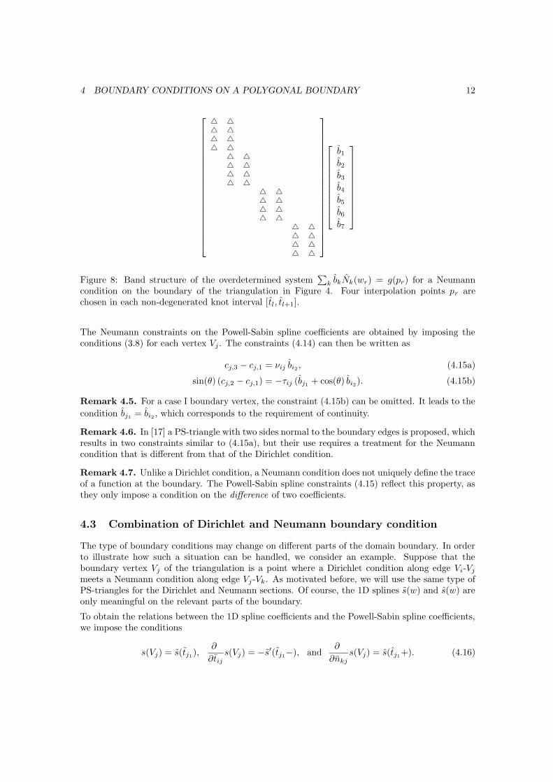
Figure 8: Band structure of the overdetermined system∑

k bkNk(wr) = g(pr) for a Neumanncondition on the boundary of the triangulation in Figure 4. Four interpolation points pr arechosen in each non-degenerated knot interval [tl, tl+1].

The Neumann constraints on the Powell-Sabin spline coefficients are obtained by imposing theconditions (3.8) for each vertex Vj . The constraints (4.14) can then be written as

cj,3 − cj,1 = νij bi2 , (4.15a)

sin(θ) (cj,2 − cj,1) = −τij (bj1 + cos(θ) bi2). (4.15b)

Remark 4.5. For a case I boundary vertex, the constraint (4.15b) can be omitted. It leads to the

condition bj1 = bi2 , which corresponds to the requirement of continuity.

Remark 4.6. In [17] a PS-triangle with two sides normal to the boundary edges is proposed, whichresults in two constraints similar to (4.15a), but their use requires a treatment for the Neumanncondition that is different from that of the Dirichlet condition.

Remark 4.7. Unlike a Dirichlet condition, a Neumann condition does not uniquely define the traceof a function at the boundary. The Powell-Sabin spline constraints (4.15) reflect this property, asthey only impose a condition on the difference of two coefficients.

4.3 Combination of Dirichlet and Neumann boundary condition

The type of boundary conditions may change on different parts of the domain boundary. In orderto illustrate how such a situation can be handled, we consider an example. Suppose that theboundary vertex Vj of the triangulation is a point where a Dirichlet condition along edge Vi-Vj

meets a Neumann condition along edge Vj-Vk. As motivated before, we will use the same type ofPS-triangles for the Dirichlet and Neumann sections. Of course, the 1D splines s(w) and s(w) areonly meaningful on the relevant parts of the boundary.

To obtain the relations between the 1D spline coefficients and the Powell-Sabin spline coefficients,we impose the conditions

s(Vj) = s(tj1),∂

∂tijs(Vj) = −s′(tj1−), and

∂

∂nkjs(Vj) = s(tj1+). (4.16)

5 BOUNDARY CONDITIONS ON CURVED DOMAINS 13

Using equations (4.8a), (4.8b) and (4.14b), one finds that (4.16) is equivalent to the constraints


cj,2 − cj,1 =2τij

λij

(bi2 − bij)

‖Vi − Vj‖, (4.17b)

cos(θ) (cj,3 − cj,1) = −νij

(

bj1 + sin(θ)2

λij

(bi2 − bij)

‖Vi − Vj‖

)

. (4.17c)

Remark 4.8. When the two boundary edges are orthogonal to each other, the third constraint(4.17c) becomes redundant and can be omitted, since

bj1 = − sin(θ)2

λij

(bi2 − bij)

‖Vi − Vj‖, (4.18)

in accordance with relation (3.9b). For θ = π/2, the reduced set of constraints simplifies to

cj,1 = bij , (4.19a)

cj,2 = bij +2τij

λij

(bi2 − bij)

‖Vi − Vj‖, (4.19b)

when we choose Qj,1 = Vj , referring to Remark 4.1.

Other types of boundary conditions that combine Dirichlet and Neumann conditions, can be treatedin a similar fashion. For example, a Cauchy boundary condition which specifies both the value(4.1) and the normal slope (4.13) at the boundary. Here, we determine the coefficients of bothsplines s(w) and s(w). During the computation of the 1D spline coefficients, we have to enforcethe relations (3.9), corresponding to the behaviour of a PS-spline. In the projection step, we nowsolve the following constrained minimization problem,

min ωD

m∑

r=1

(

f(pr) − s(wr))2

+ ωN

m∑

r=1

(

g(pr) − s(wr))2

, subject to (3.9), (4.20)

for some weights ωD and ωN . A Cauchy boundary conditions is sometimes called a weighted averageof imposing a Dirichlet and a Neumann condition. The term refers to an average that takes intoaccount the proportional relevance of each component, dependent on which information is availablefor the well-posedness of the problem and its subsequent successful solution. The correspondingset of constraints on the PS-spline coefficients is formed by (4.9a), (4.9b) and (4.15a) for eachboundary vertex Vj . Hence, the values of all coefficients associated to a boundary vertex will bedetermined.

5 Boundary conditions on curved domains

This section addresses Powell-Sabin splines with boundary conditions defined on a curved domainboundary ∂Ωc. Such a domain boundary cannot be exactly represented by a triangulation. Wesuppose that the boundary vertices of the triangulation are located on the curved line.

5.1 A Dirichlet boundary condition

We try to impose a Dirichlet boundary condition on a Powell-Sabin spline, i.e. (4.1), where thefunction f(x, y) is given on a curved domain boundary ∂Ωc. This introduces two kinds of errors:


V1

V2

V3

R12

Rc12

R23

Rc23

R31

Rc31

tc1/tc1

tc2

tc3/tc2

tc4tc7

tc6/tc4tc5/tc3

Figure 9: Example triangulation with knot positions for a Dirichlet (tck) and Neumann (tck) bound-ary condition, defined on a curved domain boundary.

errors caused by the quadratic nature of the spline, and errors caused by the linear approximationof the domain boundary. Contrary to the polygonal case in section 4, the PS-spline is not alwaysdefined along the boundary of the physical domain, i.e., when the boundary curve lies outside thetriangulation. In addition, if the curve is inside, the behaviour of the Powell-Sabin spline alongthe trace of the curve depends on the type of the curve. For instance, the spline behaves as apiecewise quadratic polynomial along a linear line, and as a piecewise quartic polynomial alonga parabolic curve. As in the polygonal case we distinguish two boundary situations: a smoothcurve, i.e. C1-continuous, at vertex Vj (case Ic), and a curve with a tangential discontinuity at Vj

(case IIc). The triangulation in Figure 9 consists of two case Ic boundary vertices (V1, V2), and asingle case IIc boundary vertex (V3).

Our approach is to approximate in a first step the trace of f(x, y) along ∂Ωc by a 1D quadraticspline s(wc), e.g. with a discrete least squares method. Here, wc is the accumulated arc length incounter-clockwise direction along the boundary curve. The spline knots of s(wc) are assigned tothe vertices Vj and the interjacent points Rc

ij at the boundary curve, as illustrated in Figure 9.

Single knots, denoted as tcij , are associated with the points Rcij . Double knots, i.e. tcj1 and tcj2 ,

are assigned to the case IIc boundary vertices Vj ; a single knot tcj1 is assigned to Vj otherwise.We select the lengths of the knot intervals so that they preserve the boundary curve arc lengthsbetween the points Rc

ij and Vj .

In a second step, we compose a set of constraints on the PS-spline coefficients such that the PS-spline will approximately match s(wc). At the points Vj , we impose that the value and tangentialderivatives of the Powell-Sabin spline are equal to the value and tangential derivatives of s(wc) atthese points. I.e., we impose the conditions (4.2) where tij and tkj are the directions tangent tothe boundary curve at Vj in clockwise and counter-clockwise direction. If the boundary curve ispolygonal, these conditions ensure that s(wc) exactly matches the trace of the Powell-Sabin splinealong the boundary.

In order to simplify the constraints, we suggest to use a PS-triangle with one side parallel to tij ,and another side orthogonal to tij , as illustrated in Figure 10. We obtain then a set of constraints


Vi

Rij

Vj

Rjk Vk

Rcij

Rcjk

Z

Qj,2 Qj,1

Qj,3

(a) case Ic boundary

Vi

Rij

Vj Rjk

Vk

Rcij

Rcjk

Z

Qj,2

Qj,3

Qj,1

(b) case IIc boundary

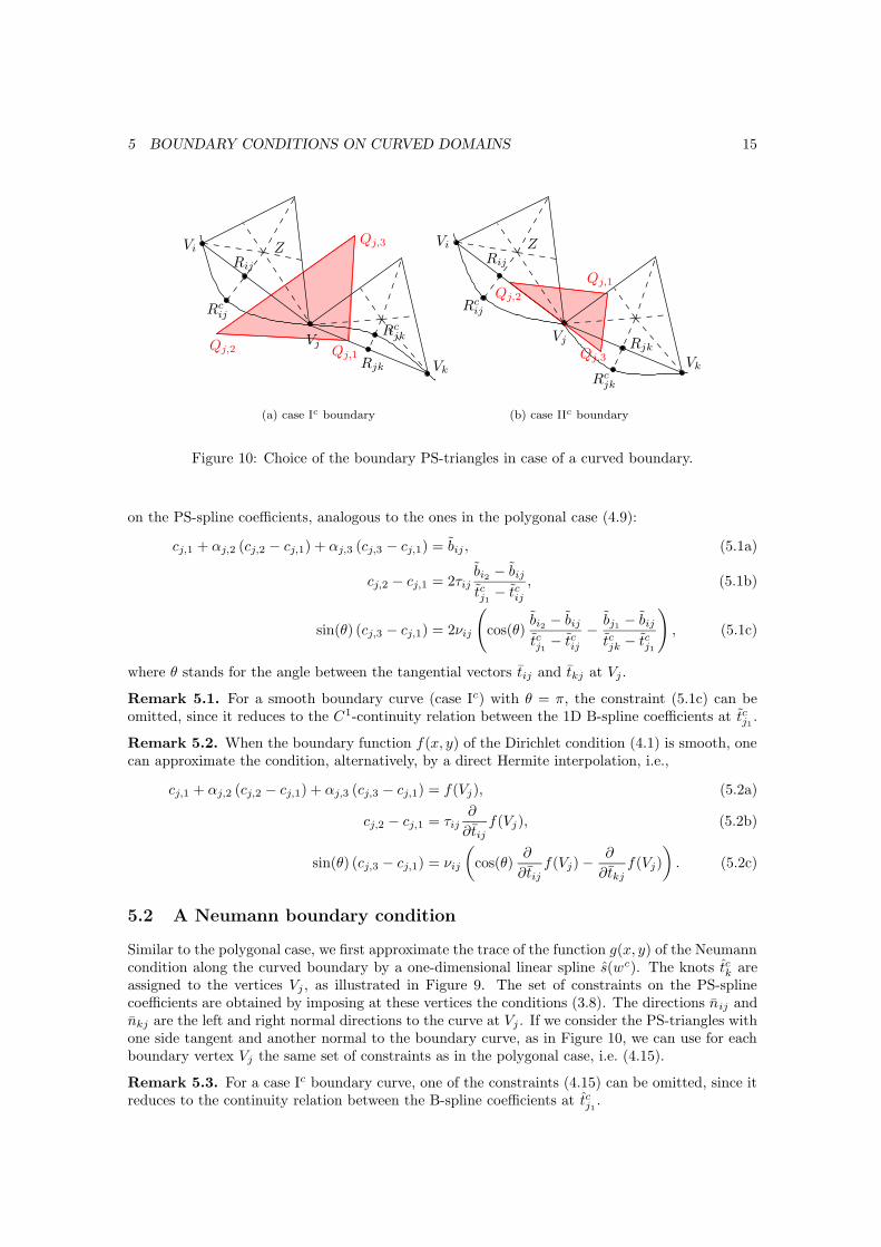
Figure 10: Choice of the boundary PS-triangles in case of a curved boundary.

on the PS-spline coefficients, analogous to the ones in the polygonal case (4.9):


cj,2 − cj,1 = 2τijbi2 − bij

tcj1 − tcij, (5.1b)

sin(θ) (cj,3 − cj,1) = 2νij

(

cos(θ)bi2 − bij

tcj1 − tcij− bj1 − bij

tcjk − tcj1

)

, (5.1c)

where θ stands for the angle between the tangential vectors tij and tkj at Vj .

Remark 5.1. For a smooth boundary curve (case Ic) with θ = π, the constraint (5.1c) can beomitted, since it reduces to the C1-continuity relation between the 1D B-spline coefficients at tcj1 .

Remark 5.2. When the boundary function f(x, y) of the Dirichlet condition (4.1) is smooth, onecan approximate the condition, alternatively, by a direct Hermite interpolation, i.e.,

cj,1 + αj,2 (cj,2 − cj,1) + αj,3 (cj,3 − cj,1) = f(Vj), (5.2a)

cj,2 − cj,1 = τij∂

∂tijf(Vj), (5.2b)

sin(θ) (cj,3 − cj,1) = νij

(

cos(θ)∂

∂tijf(Vj) −

∂

∂tkjf(Vj)

)

. (5.2c)

5.2 A Neumann boundary condition

Similar to the polygonal case, we first approximate the trace of the function g(x, y) of the Neumanncondition along the curved boundary by a one-dimensional linear spline s(wc). The knots tck areassigned to the vertices Vj , as illustrated in Figure 9. The set of constraints on the PS-splinecoefficients are obtained by imposing at these vertices the conditions (3.8). The directions nij andnkj are the left and right normal directions to the curve at Vj . If we consider the PS-triangles withone side tangent and another normal to the boundary curve, as in Figure 10, we can use for eachboundary vertex Vj the same set of constraints as in the polygonal case, i.e. (4.15).

Remark 5.3. For a case Ic boundary curve, one of the constraints (4.15) can be omitted, since itreduces to the continuity relation between the B-spline coefficients at tcj1 .

6 NUMERICAL EXAMPLES 16

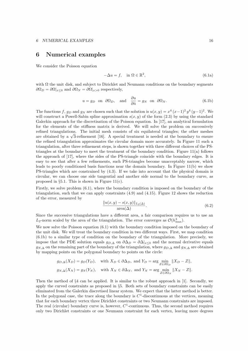
6 Numerical examples

We consider the Poisson equation

−∆u = f, in Ω ∈ R2, (6.1a)

with Ω the unit disk, and subject to Dirichlet and Neumann conditions on the boundary segments∂ΩD = ∂Ω|x≤0 and ∂ΩN = ∂Ω|x>0 respectively,

u = gD on ∂ΩD, and∂u

∂n= gN on ∂ΩN . (6.1b)

The functions f , gD and gN are chosen such that the solution is u(x, y) = x4 (x−1)2 y4 (y−1)2. Wewill construct a Powell-Sabin spline approximation s(x, y) of the form (2.3) by using the standardGalerkin approach for the discretisation of the Poisson equation. In [17], an analytical formulationfor the elements of the stiffness matrix is derived. We will solve the problem on successivelyrefined triangulations. The initial mesh consists of six equilateral triangles; the other meshesare obtained by a

√3-refinement [16]. A special treatment is needed at the boundary to ensure

the refined triangulation approximates the circular domain more accurately. In Figure 11 such atriangulation, after three refinement steps, is shown together with three different choices of the PS-triangles at the boundary to meet the treatment of the boundary condition. Figure 11(a) followsthe approach of [17], where the sides of the PS-triangle coincide with the boundary edges. It iseasy to see that after a few refinements, such PS-triangles become unacceptably narrow, whichleads to poorly conditioned basis functions near the domain boundary. In Figure 11(b) we showPS-triangles which are constrained by (4.3). If we take into account that the physical domain iscircular, we can choose one side tangential and another side normal to the boundary curve, asproposed in §5.1. This is shown in Figure 11(c).

Firstly, we solve problem (6.1), where the boundary condition is imposed on the boundary of thetriangulation, such that we can apply constraints (4.9) and (4.15). Figure 12 shows the reductionof the error, measured by

‖u(x, y) − s(x, y)‖L2(∆)

area(∆). (6.2)

Since the successive triangulations have a different area, a fair comparison requires us to use anL2-norm scaled by the area of the triangulation. The error converges as O(h3

max).

We now solve the Poisson equation (6.1) with the boundary condition imposed on the boundary ofthe unit disk. We will treat the boundary condition in two different ways. First, we map condition(6.1b) to a similar type of condition on the boundary of the triangulation. More precisely, weimpose that the PDE solution equals gD,∆ on ∂∆D = ∂∆|x≤0 and the normal derivative equalsgN,∆ on the remaining part of the boundary of the triangulation, where gD,∆ and gN,∆ are obtainedby mapping points on the polygonal boundary to points on the circle:

gD,∆(XD) = gD(YD), with XD ∈ ∂∆D, and YD = arg minZ∈∂ΩD

‖XD − Z‖,

gN,∆(XN ) = gN (YN ), with XN ∈ ∂∆N , and YN = arg minZ∈∂ΩN

‖XN − Z‖.

Then the method of §4 can be applied. It is similar to the robust approach in [1]. Secondly, weapply the curved constraints as proposed in §5. Both sets of boundary constraints can be easilyeliminated from the Galerkin discretised linear system. We expect that the latter method is better.In the polygonal case, the trace along the boundary is C1-discontinuous at the vertices, meaningthat for each boundary vertex three Dirichlet constraints or two Neumann constraints are imposed.The real (circular) boundary curve is, however, C1-continuous. Thus, the second method requiresonly two Dirichlet constraints or one Neumann constraint for each vertex, leaving more degrees

6 NUMERICAL EXAMPLES 17

−1.2 −1 −0.8 −0.6 −0.4 −0.2 0 0.2 0.4 0.6 0.8 1 1.2−1.2

−1

−0.8

−0.6

−0.4

−0.2

0

0.2

0.4

0.6

0.8

1

1.2

(a) Choice of the PS-triangles in case of a polygonalboundary, following the approach of [17].

−1.2 −1 −0.8 −0.6 −0.4 −0.2 0 0.2 0.4 0.6 0.8 1 1.2−1.2

−1

−0.8

−0.6

−0.4

−0.2

0

0.2

0.4

0.6

0.8

1

1.2

(b) Choice of the PS-triangles in case of a polygonalboundary, as proposed in §4.

−1.2 −1 −0.8 −0.6 −0.4 −0.2 0 0.2 0.4 0.6 0.8 1 1.2−1.2

−1

−0.8

−0.6

−0.4

−0.2

0

0.2

0.4

0.6

0.8

1

1.2

(c) Choice of the PS-triangles in case of a circularboundary, as in §5.

−1.2 −1 −0.8 −0.6 −0.4 −0.2 0 0.2 0.4 0.6 0.8 1 1.2−1.2

−1

−0.8

−0.6

−0.4

−0.2

0

0.2

0.4

0.6

0.8

1

1.2

(d) Choice of the collocation points, based on thepositions of the maxima of the PS B-splines.

Figure 11: Choice of PS-triangles in case of (a)-(b) a polygonal boundary, and (c) a curved bound-ary. (d) Possible placement of the collocation points for the mesh and the PS-triangles in (c),based on the positions of the maxima of the Powell-Sabin B-splines..

of freedom to satisfy (6.1). Figure 12 shows the reduction of the error for both approaches. Thesecond approach leads to a more accurate solution, with the expected order of convergence.

In a Galerkin finite element approach for solving differential equations, a Neumann condition doesnot strictly need to be enforced on the elements of the approximation space. As natural boundaryconditions, they are usually satisfied automatically. Enforcing a Neumann condition explicitly onthe elements of the approximation space is nevertheless useful in, e.g., collocation methods. Thecollocation method has several advantages to the Galerkin method: no expensive scalar products

7 CONCLUDING REMARKS 18

0 1 2 3 4 5 6 7 810

−7

10−6

10−5

10−4

10−3

10−2

10−1

100

101

level of refinement

erro

r

(a) Galerkin + polygonal boundary, polygonal constraints(b) Galerkin + curved boundary, polygonal constraints(c) Galerkin + curved boundary, curved constraints(d) Collocation + curved constraintsO(h

max3 )

Figure 12: Using successively√

3-refined meshes approximating a unit disk, as in Figure 11, thenorm of the error (6.2) for PDE (6.1) is showed in case the boundary condition is treated on theboundary of the triangulation (a), compared with three treatments on the real (curved) boundary(b)-(d). The Galerkin (a)-(c) and collocation (d) discretisation is considered.

have to be calculated, and the system of equations is a lot more sparse. To ensure the existence ofa solution, there must lie at least three collocation points in the molecule of each vertex, except atthe boundary vertices where the number dependents on the kind of boundary condition. To satisfythe above requirement, one can place the collocation points at the positions of the maxima of thenormalized Powell-Sabin B-splines, as illustrated in Figure 11(d). Figure 12 shows the reductionof the error for the collocation method applied to (6.1). Despite the advantages, spline collocationmethods are not extensively used. An optimal placement of the collocation points is not trivial,and is only derived for certain degree splines on rectangular grid discretisations [2].

7 Concluding remarks

In this paper we addressed the question of how to impose boundary conditions on Powell-Sabinsplines. We showed that imposing boundary conditions leads to sets of simple constraints onthe PS-spline coefficients. We discussed Dirichlet and Neumann boundary conditions, definedon polygonal and non-polygonal domains. The general principle is twofold: first we project theboundary function to a one-dimensional spline space, and then the constraints on the PS-splinecoefficients are determined.

A careful choice of the PS-triangles at the boundary can simplify the boundary constraints. Weadvocate a PS-triangle with one side tangential and another normal to the boundary curve. Otherparticular choices, as proposed in [17], can lead to some simpler constraints. Yet, our type ofboundary PS-triangle has the advantage that the corresponding basis functions are always wellconditioned, also when the boundary edges of the triangulation have an angle close to π. Inaddition, since we use the same type of PS-triangles regardless of the type of boundary condition,we can construct the basis in advance, irrespective of the particular application.

REFERENCES 19

Acknowledgement

Hendrik Speleers is funded as a Research Assistant of the Fund for Scientific Research Flanders(Belgium).

References

[1] J.H. Bramble and J.T. King. A robust finite element method for non-homogeneous Dirichletproblems in domains with curved boundaries. Math. Comput., 63(207):1–17, 1994.

[2] C.C. Christara. Quadratic spline collocation methods for elliptic partial differential equations.BIT, 34(1):33–61, 1994.

[3] C.K. Chui and L.L. Schumaker. On spaces of piecewise polynomials with boundary conditionsI. Rectangles. In W. Schempp and K. Zeller, editors, Multivariate Approx. Theory II, pages69–80, Basel, 1982. Birckhauser.

[4] C.K. Chui, L.L. Schumaker, and R.H. Wang. On spaces of piecewise polynomials with bound-ary conditions II. Type-1 triangulations. In Z. Ditzian, A. Meir, S. Riemenschneider, andA. Sharma, editors, Second Edmonton Conf. on Approx. Theory, pages 51–66, Providence,1983. AMS.

[5] C.K. Chui, L.L. Schumaker, and R.H. Wang. On spaces of piecewise polynomials with bound-ary conditions III. Type-2 triangulations. In Z. Ditzian, A. Meir, S. Riemenschneider, andA. Sharma, editors, Second Edmonton Conf. on Approx. Theory, pages 67–80, Providence,1983. AMS.

[6] C. de Boor. On calculating with B-splines. J. Approx. Theory, 6:50–62, 1972.

[7] P. Dierckx. Curve and Surface Fitting with Splines. Oxford University Press, Oxford, 1993.

[8] P. Dierckx. On calculating normalized Powell-Sabin B-splines. Comput. Aided Geom. Design,15(3):61–78, 1997.

[9] P. Dierckx, S. Van Leemput, and T. Vermeire. Algorithms for surface fitting using Powell-Sabin splines. IMA J. Numer. Anal., 12:271–299, 1992.

[10] K. Hollig, U. Reif, and J. Wipper. Weighted extended B-spline approximation of Dirichletproblems. SIAM J. Numer. Anal., 39(2):442–462, 2001.

[11] C. Manni and P. Sablonniere. Quadratic spline quasi-interpolants on Powell-Sabin partitions.Technical Report IRMAR 04-16, 2004.

[12] M.J.D. Powell and M.A. Sabin. Piecewise quadratic approximations on triangles. ACM Trans.

Math. Softw., 3:316–325, 1977.

[13] V.L. Rvachev and T.I. Sheiko. R-functions in boundary value problems in mechanics. Appl.

Mech. Rev., 48(4):151–188, 1995.

[14] V. Shapiro and I. Tsukanov. Meshfree simulation of deforming domains. Comput. Aided

Design, 31:459–471, 1999.

[15] X. Shi, S. Wang, W. Wang, and R.H. Wang. The C1-quadratic spline space on triangulations.Technical Report 86004, Dep. Math., Jilin University, Changchun, 1986.

REFERENCES 20

[16] H. Speleers, P. Dierckx, and S. Vandewalle. Local subdivision of Powell-Sabin splines. Comput.

Aided Geom. Design, accepted, 2006.

[17] H. Speleers, P. Dierckx, and S. Vandewalle. Numerical solution of partial differential equationswith Powell-Sabin splines. J. Comput. Appl. Math., 189(1-2):643–659, 2006.

[18] E. Vanraes, J. Maes, and A. Bultheel. Powell-Sabin spline wavelets. Int. J. Wavets Multires.

Information Processing, 2(1):23–42, 2004.

[19] K. Willemans and P. Dierckx. Constrained surface fitting using Powell-Sabin splines. In P.J.Laurent, A. Le Mehaute, and L.L. Schumaker, editors, Proceedings of Wavelets, Images and

Surface Fitting, Second Int. Conf. on Curves and Surfaces, pages 511–520, Chamonix-MontBlanc, France, 1994. Wellesley.

Powell–Sabin splines with boundary conditions for polygonal and non-polygonal domains

Documents