Poverty Dynamics in Four OECD Countries

Unclassified ECO/WKP(99)4

Organisation de Coopération et de Développement Economiques OLIS : 23-Apr-1999Organisation for Economic Co-operation and Development Dist. : 30-Apr-1999__________________________________________________________________________________________

English text onlyECONOMICS DEPARTMENT

POVERTY DYNAMICS IN FOUR OECD COUNTRIESECONOMICS DEPARTMENT WORKING PAPERS N0. 212

byPablo Antolín, Thai-Thanh Dang and Howard OxleyAssisted by Ross Finnie and Roger Sceviour

Unclassified

EC

O/W

KP

(99)4E

nglish text only

Most Economics Department Working Papers beginning with No. 144 are now available throughOECD’s Internet Web site at http://www.oecd.org/eco/eco.

77151

Document complet disponible sur OLIS dans son format d’origine

Complete document available on OLIS in its original format

ECO/WKP(99)4

2

ABSTRACT/RESUME

This study examines the dynamics of poverty for four OECD countries (Canada, Germany, theUnited Kingdom and the United States). It provides information on patterns of poverty, which groups stayin poverty the longest, and household/individual characteristics and life-course events which appear to bemost closely associated with transitions into and out of poverty and the length of time individuals stay inpoverty. The analysis finds that the number of people touched by poverty over a six year period issignificantly larger that the poverty rate might suggest, but the share of those staying poor for a long timeis much smaller. The data suggest that longer-term poor are concentrated among women, lone parents andolder single individuals. The study finds that employment status is the main factor affecting transitions intoand out of poverty and the duration of poverty.

****

Cette étude examine la dynamique de la pauvreté dans quatre pays de l’OCDE (Canada, Allemagne,Royaume Unis et États Unis). Elle fournit des informations détaillées sur la structure de la pauvreté, lesgroupes qui se trouvent dans la pauvreté de longue durée, les caractéristiques des ménages/ individus et lesévénements étroitement associés aux périodes de transitions ainsi que la longueur des périodes de pauvreté.Le nombre d’individus touchés au moins une fois par la pauvreté au cours des 6 dernières années est plusimportant que ne le suggèrent les taux de pauvretés statiques. En revanche, les individus subissant un étatde pauvreté persistante s’avèrent être moins nombreux. Les données montrent que les femmes, les famillesmonoparentales et les retraités vivant seuls sont plus fortement concentrés dans la pauvreté de longuedurée. Enfin, parmi les facteurs analysés, l’emploi et ses changements apparaissent comme déterminant surles mouvements d’entrée et de sortie ainsi que sur la durée des périodes de pauvreté.

Copyright: OECD, 1999 Applications for permission to reproduce or translate all, or part of, thismaterial should be made to: Head of Publications Service, OECD, 2 rue André-Pascal, 75775PARIS CEDEX 16, France

ECO/WKP(99)4

3

TABLE OF CONTENTS

POVERTY DYNAMICS IN FOUR OECD COUNTRIES............................................................................ 5

1. Introduction............................................................................................................................................ 51.1 Main results ....................................................................................................................................... 6

2. Defining income and poverty and the data sources................................................................................ 72.1 Definition of income and poverty...................................................................................................... 72.2 Data sources and issues ..................................................................................................................... 7

3. The dynamics of poverty over a six-year period.................................................................................... 93.1 Broad patterns of poverty dynamics.................................................................................................. 93.2 Poverty dynamics before and after taxes and transfers ................................................................... 113.3 The characteristics of the poor by length of spell............................................................................ 12

4. Factors associated with poverty transitions.......................................................................................... 134.1 How much does income change during transitions? ...................................................................... 134.2 “Events” and transitions................................................................................................................. 144.3 Which “events” have households experienced when they enter and exit poverty.......................... 154.4 “Events” and the probability of transitions.................................................................................... 16

5. How long do people stay in poverty?................................................................................................... 185.1 Data and methodology..................................................................................................................... 185.2 What determines the length of time people stay in poverty?......................................................... 185.3 Re-entry into poverty...................................................................................................................... 21

6. Conclusion........................................................................................................................................... 21

...................................................................................................................................................................... 22

BIBLIOGRAPHY......................................................................................................................................... 23

ANNEX 1: TECHNICAL NOTES.............................................................................................................. 46

1. Data sources and methodology............................................................................................................ 461.1. Data sources.................................................................................................................................. 461.2. Defining poverty thresholds.......................................................................................................... 471.3. Characteristics of the non-poor, shorter-term poor and longer-term poor (Table 3)..................... 48

2. Analysis of transitions into and out of poverty.................................................................................... 522.1. The data set/sample....................................................................................................................... 522.2. Construction of Tables 4 to 7........................................................................................................ 532.3. Estimates of the probability of exit and entry (Table 8)................................................................ 57

3. The persistence of poverty: duration models...................................................................................... 703.1. The sample.................................................................................................................................... 703.2. The model...................................................................................................................................... 703.3. Comments on the explanatory variables and estimations.............................................................. 74

ECO/WKP(99)4

4

Tables and Figures

1a. Poverty rates, gross rates of entry and exit and the share of individuals in povertyover a six-year period

1b. Total time over a six-year period that individuals spend in poverty2. Dynamics of poverty: empirical probabilities of exit and re-entry conditional on duration3. Characteristics of the non-poor, shorter-term poor and longer-term poor4. Distribution of transitions by size of income change5. Frequency of poverty-related events by income component6. Frequency of “events” associated with poverty transitions7. Frequency of “events” associated with poverty transitions: by family type8. “Events” associated with entry into and exit from poverty: logit estimates9. Estimates of exit rates from poverty by length of time spent in poverty10. Percentage of people remaining in poverty11. Average duration in poverty according to certain household characteristics12. Estimates of poverty re-entry by length of time spent out of poverty

Figure

1. Three dimensions of poverty

Tables of Annex 1

A1. Characteristics of the non-poor, shorter-term poor and longer-term poor: Total population andworking-age population

A2. Frequency of poverty-related “events”: further decomposition of the main categories of “events”A3. Entry model: crossed variablesA4. Exit model: crossed variablesA5. Entry model: uncrossed variablesA6. Exit model: uncrossed variablesA7. Logit estimates of the probability of exiting poverty conditional on durationA8. Logit estimates of the probability of re-entering poverty conditional on duration

Boxes

A1. Variables defined in the sampleA2. Logit modelsA3. The analytical modelA4. Explanatory variables for estimates of the duration of poverty and re-entry

ECO/WKP(99)4

5

POVERTY DYNAMICS IN FOUR OECD COUNTRIES

Pablo Antolín, Thai-Thanh Dang and Howard OxleyAssisted by Ross Finnie and Roger Sceviour1,2

1. Introduction

1. Poverty rates are helpful indicators of the level of poverty in a country during a specific period oftime. However, they do not provide important information about the extent of mobility into and out ofpoverty or about the length of time people remain in poverty. Whether an individual suffers poverty over along period of time or a short period is not the same and the policy response is likely to differ.

2. The present study complements and extends previous work on trends in income distribution andpoverty (Oxley et al., 1999) by examining more closely the dynamics of poverty. This study useslongitudinal data sets, which follow individuals over time and permit flows into and out of poverty and thelength of stay below the poverty threshold to be estimated. Since these data sets also contain informationon individual and household characteristics, they can suggest which types of individual stay longest belowthe poverty threshold and whether certain changes in household status -- such as getting or losing a job orexperiencing divorce -- are associated with transitions into or out of poverty.

3. This study examines the following subject areas, for four OECD countries for which suitablelongitudinal data were available (Canada, Germany, the United Kingdom and the United States):

− flows into and out of poverty and “events” most closely associated with those transitions;

− which groups make up the short and longer-term poor;

− factors affecting the length of time individuals stay in poverty and the risk that people fallback into poverty.

4. These issues are examined in two ways. First, tabulations give broad orders of magnitude of theflows into and out of poverty, the “events” associated with these transitions, the characteristics of the poor,the duration of poverty spells and the extent of subsequent re-entry into poverty. Second, econometrictechniques allow a more precise evaluation of the factors associated with transitions, the duration of spellsand the probability of re-entry. However, while these analyses provide a useful characterisation of thenature of poverty, there is no attempt to model household and individual behaviour which underlietransitions into and out of poverty. Thus, conclusions that purport to deal with structural relationships

1. This study was prepared by Pablo Antolin, Thai Thanh Dang and Howard Oxley from the Economics

Department of the OECD. Data for Canada were prepared by Ross Finnie from Queens University andRoger Scerviour from Statistics Canada. Ross Finnie also provided numerous helpful suggestionsconcerning the project. The contact person is Howard Oxley who can be reached at (331) 45 24 87 92(Fax: 33 1 44 30 63 83) or at [email protected]

2. This study benefited from helpful comments from Jorgen Elmeskov; Mike Feiner; Bob Ford; StephenJenking; Flip de Kam; Mark Pearson, Paul Swaim and numerous members of the Economics Departmentat the OECD and participants of the UK Treasury Workshop on Persistent Poverty and Lifetime Inequality17th and 18th November 1998. Jackie Gardel and Muriel Duluc provided excellent secretarial support.The views are those of the authors and should not be attributed to the OECD.

ECO/WKP(99)4

6

-- between poverty programmes and transitions into or out of poverty, for example -- need to be drawnwith great care. In addition, cross-country comparability of the data is limited, providing another reason toexercise caution in interpreting the results.

5. The paper is organised as follows. A summary of the main results is presented immediatelybelow. A number of issues concerning the definition of income, poverty and peculiarities of the data setsare then briefly addressed in Section 2. This is followed, in Section 3, by an overview of the variousfactors affecting poverty transitions using some broad indicators of poverty inflows, outflows and durationacross countries. Section 4 looks in greater detail at the factors associated with poverty transitions, whileSection 5 examines duration and re-entry. Section 6 concludes. Additional technical material is presentedin Annex 1, covering data sources, methodology and more detailed results.

1.1 Main results

6. Key results of this study are:

- Between 20 and just under 40 per cent of the population is touched by poverty over a six-yearperiod, a much larger portion than would be suggested by the “static” poverty rates. Withinthis group, however, the majority have short spells. As spells lengthen, the probability of exitfalls such that a small group of the population remains in poverty for long periods of timewith, apparently, little chance of exit.

- The probability of exiting poverty falls with previous experiences in poverty. At the sametime, there is a high probability of falling back into poverty. Thus, for the longer-term poor,low probability of exit and high probability of re-entry tend to reinforce each other. Peoplewith six or more years in poverty (i.e. the longer-term poor) typically make up 2-6 per cent ofthe population. However, because of their long stays in poverty they represent aroundone-third of the total time all individuals spend in poverty (from 30 to just over 50 per cent iffive or more years are considered).

- The tax and transfer system sharply reduces poverty rates, particularly as regards longer-termpoverty. The difference in poverty rates pre- and post-taxes-and-transfers is smallest in theUnited States.

- For three of the four countries, the characteristics of households experiencing shorter spellsin poverty tend to be different from those of the longer-term poor. A large share of thelonger-term poor would appear to be women, lone parents and elderly single individuals. Asignificant share of the longer-term poor work.

- Obtaining or losing employment is particularly important for transitions into and out ofpoverty. Gaining employment is the main factor in reducing the length of time spent inpoverty. Some aspects of this are:

- A large share of transitions occurs when there are employment/earnings-related “events”,particularly in the case of exits from poverty. The probability of transiting into poverty isgenerally higher for employment-related “events” than for family-related “events”.

- Households with more than one worker are better protected from poverty and have shorterstays in poverty. Increased employment or hours worked by other household members isan important source of exit from poverty and households which get a second job appear toshorten their poverty spells by more than households which obtain a first job.

ECO/WKP(99)4

7

Multiple-earner households may be capable of adjusting labour supply more easily tocompensate for job loss or lower earnings of other household members.

- Separations and divorce are more important for poverty entry than marriage is for povertyexit and the length of stays for female-headed lone-parent households is significantly longerthan other household groups. Employment is the main channel for exit of lone-parenthouseholds from poverty and acts to reduce the average length of stay significantly.

2. Defining income and poverty and the data sources

2.1 Definition of income and poverty

7. Following the methodology in OECD (1997a), the focus of attention is the individual (includingchildren), but the unit for calculating income is the household. Individuals are assumed to receive theequivalent disposable income of the household to which they belong. Equivalent income is householddisposable income -- i.e. market income and transfers from government less direct taxes and social securitypayments of all household members -- divided by the square root of the number of individuals in thehousehold. The division by a number less than the size of the household is intended to take account ofhousehold economies of scale (see Annex 1, Section 1). This adjustment involves an important element ofjudgement but has been widely used in other international comparative studies.

8. To assess the direct impact of the tax and transfer system, the transitions have also beencalculated, in some cases, using market income –- i.e. disposable income plus taxes paid to and lesstransfers received from government -- but using the poverty threshold calculated with householddisposable income. The differences in transitions give some indication of the relative importance ofmarket income and the tax and transfer system in exits from poverty. Indirect effects such as whenincentives arising from the tax and transfer system affect behaviour and therefore market income, could notbe isolated.

9. The distribution of income is constructed by ranking individuals on the basis of their equivalentincome. The poverty threshold was established at 50 per cent of the median equivalent disposable income,a threshold which, once again, has been widely used in international comparative studies. Poverty rates3

presented in OECD (1997a) indicated that using other definitions would significantly affect the level ofpoverty, but that the trends over time were broadly unchanged. However, where a large number ofindividuals are grouped in certain segments of the distribution, the pattern of poverty dynamics could beaffected4.

2.2 Data sources and issues

10. The focus of this study is not the level of poverty, but the dynamics and persistence of poverty-- i.e. the flows into and out of poverty and the time spent in poverty. Such work requires data sets thatfollow individuals through time (panels). Individuals are characterised in two ways: first, in terms ofpersonal characteristics -- for example, age, sex and education attainment -- and, second, in terms of

3. Defined as the head-count ratio or the ratio of the poor to the total population.

4. For example, Jarvis and Jenkins (1997) find rather significant differences between a relative povertythreshold and a threshold fixed in real terms due to rather a large number of individuals who lie near theauthors’ chosen poverty thresholds.

ECO/WKP(99)4

8

household characteristics -- for example, the income of other household members and the age and workattachment of the head of household. Since each individual is followed over time, these data help toidentify whether “events” -- such as changes in employment within the household -- coincide withmovements into or out of poverty. Moreover, the length of poverty spells can be determined and estimatesmade of the relationship between the length of spell and individual or household characteristics.

11. Relatively few OECD countries have sufficiently developed data sets of this kind. This gap isbeing rapidly filled in many countries -- for example, in Europe through the Eurostat European panel -- butavailable time spans are generally too short for the kind of analysis carried out here. In some cases, thesample sizes of existing data sets proved too small (Italy), the data contained in them were not sufficientlydetailed through time (Belgium, Italy) or access could not be arranged (the Netherlands). For thesereasons, the analysis in this study covers four OECD countries -- Canada, Germany, the United Kingdomand United States. While Section 1 in Annex 1 provides more information on these differences, thefollowing points are particularly important in understanding and interpreting the results presented in theremainder of this paper:

− Data for Germany, the United Kingdom5 and the United States were drawn from samplesurveys, whereas tax files were the main source for Canada. For Canada, a concept referredto as “census families” was used to define households6, the sample size is much larger, butinformation on individual and household characteristics is more limited7.

− The data for the United Kingdom cover only six years: 1991 to 1996. To preservecomparability with other countries, the descriptive sections were limited to the last six yearsof available data for all countries.

− Data for Germany and the United States were drawn from the PSID-GSOEP Equivalent filewhich has adjusted the German and US panels to make income variables more comparable.They are available up to 1993 for the United States8 and to 1996 for Germany.

− Tax models have been used by national research teams to estimate taxes for Germany, theUnited Kingdom and the United States. However, tax estimates were unavailable for the lasttwo years for the United Kingdom, necessitating the use of pre-tax data for the entireperiod9,10.

5. Data do not include Northern Ireland. Readers should note that country references in this report have been

to the United Kingdom even though the sample only covers Great Britain.

6. This includes “husbands and wives (common law or legally married) with or without their never-marriedchildren, lone parents and their never-married children, with everyone else being a non-family person”.Thus there can be several census families living in the same household -- e.g. a divorced daughter with achild living with her parents would be classified a belonging to a separate household.

7. In addition, it was not possible to trace children over time, for example, as they formed new households.

8. This means that, for the United States, the effects of recent increases in the generosity of the EarnedIncome Tax Credit (EITC), as well as increases in the federal minimum wage, cannot be seen.

9. There is a more general question as to whether estimated tax data should be used at all, because in complextax systems it becomes more difficult to accurately assess the tax liability of individual households. Whilethis problem may be less severe for comparisons of static distributions of income (as there is likely to besome averaging of the errors across individuals), it may induce more serious errors in the measurement oftransitions in individual data used here.

10. Given that the tax schedule is linear over the range where the poverty line appears, experts in the UnitedKingdom have suggested that the differences between pre- and post-tax results are likely to be small.

ECO/WKP(99)4

9

− For Canada, the data are not consistent over time: social assistance benefits wereunderestimated before 1992 because they were not taxable and hence not included whenfiling for tax. This appears to have a significant effect on poverty rates, even though thosewith no other revenue than social assistance would have incomes below the 50 per centthreshold11.

− In Sections 3 and 4, data cover the last six-year period for all four countries. Section 5 makesuse of all available years (Canada: 1986-95; Germany: 1984-96; the United Kingdom:1991-96; and the United States: 1980-93).

12. Several general points should also be noted about these data. First, the time unit is the year,which may not be the most appropriate period for policy purposes (Blank, 1989; Ruggles, 1990; CensusBureau, 1998). Indeed, many countries base access to social assistance benefits on previous monthlyincome. Thus, the poverty spells of those individuals facing poverty for a month or two, but with highenough income in the rest of the year to bring annual income above the poverty line, would be missed(although one might be less concerned about such households). Ruggles (1990) estimates that usingannual rather than monthly data could reduce the number of poverty spells by 20-25 per cent in the UnitedStates.

13. Second, due to small sample sizes for those in poverty, in particular in Germany, some problemsarise when the data are broken down by characteristic as smaller sub-samples increase the size ofsampling error.

14. Third, rates of entry into and out of poverty are cyclically sensitive (Huff Stevens, 1994;Gottschalk and Moffitt, 1994). While cyclical differences are explicitly taken into account in theeconometric analysis of Section 5, this is not the case for the descriptive presentation in Section 3.

3. The dynamics of poverty over a six-year period

3.1 Broad patterns of poverty dynamics

15. The poverty rate indicates how many are poor at a point in time. However this “snapshot” masksconsiderable turnover among the poor and variation in the time that the poor stay in poverty. This sectionpresents a fuller picture of poverty patterns over time for both at the level of market income and disposableincome.

16. Three different dimensions of poverty are shown in Figure 1 and Table 1a for the most recentsix-year period:

a) The "static" poverty rate -- calculated as the share of poor people in the total populationaveraged over the period.

b) The rate of longer-term poverty -- calculated as the share of individuals in the totalpopulation who were poor in every year through the six-year period (i.e. the “6+ years inpoverty” rate).

11. This could occur because someone may receive market income for part of the year and take up social

assistance for the remainder such that the total income is above the poverty line for the year as a whole.

ECO/WKP(99)4

10

c) The rate of those poor at least once -- calculated as the share of individuals in the totalpopulation who were poor at least once through the period (the “at least once in poverty”rate).

17. Looking first at the data on a post-tax-and-transfer basis, Figure 1 shows that the povertysituation is both better and worse than the static poverty rates suggest. On the one hand, the share ofindividuals who are poor throughout the period is low (in the range of 2 to 6 per cent of the population).On the other, the share of the population that was in poverty at least once over the six-year period is large(between 20 and 38 per cent of the population). Thus, while poverty is a short-term “event” for many, it isa much more widespread phenomenon than shown by static poverty rates. These data also suggest thatthere is considerable turnover amongst the poor and this is corroborated in the second and third panels ofTable 1a. The overall entry and exit rates12 show that 30 to 40 per cent of the pool of the poor turn overevery year during the six-year period13.

18. Against this background, Table 1b shows the distribution of total time spent in poverty. Theleft-hand panel shows the share of individuals who, over the six-year period considered, spent fromone year to five or more years in poverty14, including repeat spells in poverty. In Germany, just over 45per cent remain poor only one year, which is higher than for Canada, the United Kingdom and the UnitedStates (26 to 36 per cent). The opposite is the case for those poor for five or more periods which make up27 to 28 per cent of those touched by poverty for the latter two countries, compared with only around 15per cent for Canada and Germany.

19. The right-hand panel shows the share of the total time spent in poverty by each group. To obtainthis measure, the shares in the columns in the left-hand side panel are weighted by the length of time eachspends in poverty (one to six years) and, then, divided by the total number of years spent in poverty by thewhole population (the sum of the weighted values). This measure takes into account the fact thatindividuals who have been in poverty longer, weigh more heavily in the total number of person-years spentin poverty over the six-year “window”. The results show why the longer-term poor are so important forpolicy -- those with five or more years in poverty experience as much as 50 per cent (the United Kingdomand the United States) of the time spent in poverty over the six-year period, even though this group makesup a much smaller portion of the overall population of the poor. This group tends to suffer more frompoverty and -- where they are entitled to support -- may potentially absorb a significant larger share of thetotal spending on poverty alleviation.

20. Table 2 examines the length of time individuals who fall into poverty may expect on average toremain there (left-hand panel) and how long they stay out of poverty once they exit (right-hand panel),again on both a pre- and post-tax-and-transfer basis and for the same six-year “window”15. Both panelsshow empirical hazard rates of exit (left-hand panel) and re-entry (right-hand panel) -- i.e. the probabilityof exit from (or re-entry into) poverty at a certain period, conditional on having been in (or out of) poverty 12. Overall rates of entry and exit include, respectively, all individuals falling into poverty at time t or exiting

poverty between t and t+1 as a share of the population in period t. The inflows and outflows vary over thecycle and the data presented here are averages over the six-year period. These data consider the entiresample of those interviewed every year -- and hence are “overall” exit rates.

13. The data also show differing patterns of exits and entries over the period across countries. Poverty ratesrose in all countries except Canada (however, the fall probably reflected a discontinuity in the data).

14. In the table, 5+ is the sum of five and six years or more spent in poverty.

15. This table only includes individuals where the start of a poverty spell (left-hand panel) or the exit frompoverty (right-hand panel) can be observed -- i.e. those cases where the start of the spell can be identified.The sample is a sub-sample of the sample in Table 1, which includes all individuals interviewed in all sixyears.

ECO/WKP(99)4

11

until then. For example, the exit hazard in the second period is the share of individuals exiting poverty as afraction of those (remaining) poor at the end of the first period. A fall in these hazard rates indicates thatthe share of those who exit or re-enter declines with the length of time spent in or out of poverty –- i.e. inthe case of exit rates that people who remain have progressively a more difficult time exiting poverty, thelonger the poverty period lasts16.

21. Looking first at the post-tax-and-transfer data, Table 2 shows rapid exit for most of the poor(left-hand panel); considerable re-entry into poverty (right-hand panel); and declining probability of exit(and re-entry) as the period lengthens. The importance of re-entry confirms recent research (Gottschalkand Moffitt, 1994; Jarvis and Jenkins, 1997; Huff Stevens, 1995; and Laroche, 1997) and signalsconsiderable recycling into and out of poverty17. While cross-country comparisons are difficult becausecyclical positions differ across the four countries, Canada and Germany stand out as having particularlyhigh exit rates from poverty and lower re-entry probabilities (less so for Germany) over this period, whilethe opposite is the case for the United Kingdom and the United States.

3.2 Poverty dynamics before and after taxes and transfers

22. The tax and transfer system can affect poverty transitions in various ways:

− Transfer payments (or reduced taxes) will initially limit the fall into poverty where net taxesand transfers are generous enough to keep the household above the poverty threshold –- forexample, when individuals receive age pensions on becoming retired or insurance benefits onfalling unemployed.

− The tax and transfer system can also result in earlier exit of those having fallen into poverty-- for example, there may be delays before disability pensions are granted or olderunemployed workers in poverty may receive an age pension large enough to bring them outof poverty on reaching retirement age.

− Finally, as pointed out in OECD (1997), the differences in the tax and transfer systemsthemselves may affect pre-tax-and-transfer income. For example, generous age-relatedpensions in Germany may have allowed individuals to withdraw permanently from the labourforce, or unemployment benefits may lengthen the period of job search of those ofworking age18.

16. This can reflect either a declining probability of exit, the longer people stay in poverty, for example

because of wastage of their human capital or a sorting process in which those with the best chances ofexiting exit first.

17. The following provides an example of the combined effect of results for exit and re-entry in Table 2. Theleft-hand panel shows that between 46 per cent (the United States) and 56 per cent (Canada) of thoseentering poverty would have left by the end of the first year. On the basis of information in the right-handpanel, between 36 per cent (Canada) and 64 per cent (the United States) of these individuals would havefallen back into poverty for at least one year in the following four years.

18. In some cases, cross-country variation in the difference between pre- and post-tax-and-transfer rates mayreflect institutional differences in pension arrangements. In the United States, a larger share of pensionsare employer-related than in Germany, thus raising US incomes before tax and transfers. In this case,poverty rates pre-tax-and-transfers for the retired would be lower in the United States than in Germany, allelse held equal.

ECO/WKP(99)4

12

23. A comparison of the top and bottom panels of Tables 1a, 1b and 2 and Figure 1 suggests that thetax-and-transfer system has a substantial impact on the level of poverty, the time spent in poverty and onthe rate of exit from poverty19. The left-hand panel of Table 1a confirms the results of OECD (1997) thattaxes and transfers sharply reduce the pool of the poor in all four countries -- defined in terms of the samepoverty threshold. Not surprisingly, the effect is smallest in the United States while, in the remainingthree countries, the difference between poverty rates before and after taxes and transfers is roughlythree times as large. A comparison of the top and bottom panels of Figure 1 shows the particularly markeddifference in the share of the longer-term poor in Canada, Germany and the United Kingdom –- in the firsttwo countries the rate falls from around 14 per cent to around 2 per cent.

24. Comparing the pre- and post-tax-and-transfer data in Table 1b shows that, in all countries, theshare of those remaining in poverty over the longer term is smaller after taxes and transfers. On apre-tax-and-transfer basis, the share of total time spent below the poverty threshold over a longer periodrises to between two-thirds and three-quarters of the total time all individuals spend on poverty (Table 1b,right panel). The rate at which individuals exit from poverty falls more sharply when moving from a post-tax-and-transfers to a pre-tax-and-transfer basis (although, once again, this is less the case for theUnited States) (Table 2, bottom panel). The difference pre- and post-tax-and-transfers is less marked forre-entry rates.

25. One interpretation of these results is that the tax and transfer system both reduces poverty andshortens poverty stays as well, with this effect increasing with the size of income-support programmes.However, changes in household behaviour in countries with more generous transfer systems could, inprinciple, also lead to an increase in the degree of poverty and the length of poverty stays on a pre-tax andtransfer basis, though there is limited evidence to support this hypothesis in the data presented here. In anycase, cross-country comparisons need to be treated with caution as cyclical differences have not been takeninto account.

3.3 The characteristics of the poor by length of spell

26. Variation in family and labour-market characteristics between groups of longer-term poor,shorter-term poor and non-poor -- while not implying that these differences have caused longer or shorterstays in poverty -- may provide some guidance in the formulation of anti-poverty policies. Table 3compares the share of individuals with specific characteristics across four groups for all countries: the totaland the non-poor populations, the short-term poor (individuals experiencing only one year in poverty overthe period) and the long-term poor (individuals who are poor for at least six years)20.

27. Several broad patterns appear from Table 3 (and Table A1 in Annex 1 for the populationbelonging to households with a working-age head), although they do not necessarily apply to all countriesin all cases:

19. As shown by Figure 1, the pre-tax-and-transfer poor population is larger than the post-tax-and-transfer

population, and includes: a) all those poor on a post-tax-and-transfer basis (but most of whom will nowhave a lower pre-tax-and-transfer income); and b) all those who are kept out of poverty by thetax-and-transfer system. They are thus not the same sample.

20. Characteristics are defined at the beginning of the period. Table A1 in Section 1 of Annex 1 presents:a) the same breakdown by characteristics for the population living in households with a working-age head;and b) data for population, the non-poor and the longer-term poor at the beginning and end of the six-yearperiod. A comparison of the two years indicated considerable change in the results for some characteristicsbetween the two years (particularly for the age of the household head). However, these differences do notseem large enough to change the conclusions.

ECO/WKP(99)4

13

− First, the following groups tend to be over-represented among the longer-term poor: thoseliving in female-headed households, in single-adult households with children, in householdsheaded by an individual in retirement age, in households where the head has lower education(Germany excluded21), and in households where there is no worker (and also one worker inCanada and the United States). The concentration of the longer-term poor among thesegroups probably reflects the fact that many of these conditions, when they occur, tend to lastfor a long time: for example, in the United Kingdom, lone-parenthood lasts, on average, foraround six years (McKay, 1998) and for, older people, incomes change little over time, suchthat those in poverty tend to stay there for a long period (Census Bureau, 1998).

− Second, there are significant differences between the shorter and the longer-term poor and, onsome characteristics, the short-term poor appear to be closer to the non-poor than to thelonger-term poor. In particular, the short-term poor have a considerably larger share ofhouseholds with at least one earner and are less concentrated among households which areheaded by women, single adults, lone parents and the less educated. Thus, they appear tocome from a wider span of the population.

− Finally, key characteristics of the longer-term poor tend to differ across countries: in bothGermany and the United States, women-headed households and lone parents appearparticularly important. However, in the United States around 50 percent of the longer-termpoor belong to households with at least one worker, as compared with only around 25 percent in Germany22. In Canada, over 60 per cent of the long term poor belong to householdswith at least one worker. In the United Kingdom, key features are the concentration of thelonger-term poor in non-working households, female-headed households, among householdsheaded by an elderly person and among single adults.

4. Factors associated with poverty transitions

4.1 How much does income change during transitions?

28. An initial question concerns the size of the income changes when transitions occur. Smallmovements in income of households clustered near the poverty thresholds may lead to many transitionsinto and out of poverty, but these may not be economically or socially significant. Hence, the distributionof income changes by size are of interest and these are shown in Table 4 in the form of transition matricesfor entry and exit. Each cell shows the share of individuals who shift from an originating income rangerelative to the poverty threshold (shown in the first column) to the ending income range (shown in the firstrow). For example, the cell in the first column and first row shows the share of individuals who enterpoverty with incomes between the poverty threshold and 10 per cent above the poverty threshold beforetransition, and between the poverty threshold and 10 per cent below the poverty threshold after the

21. This may reflect the fact that the education attainment variables (which refer to the head of household) may

be a poor measure of total human capital. This may be particularly the case in Germany, where on-the-jobtraining and apprenticeships may make up a larger share of total investment in skills. This may lead to anoverestimate of the share of individuals with skills corresponding to “low education”.

22. However, the problem of the working poor appears more severe in the United States where there is anon-negligible share of two-earner households who were poor through the period.

ECO/WKP(99)4

14

transition. This particular group is one measure of “noise” -- i.e. the number of poverty transitions whichresult from relatively small changes in income around the poverty line23.

29. The results show:

− That “noise” represents a small part (6 to 9.5 per cent) of total transitions.

− The bulk of transitions do occur in a range of between 66 per cent and 150 per cent of thepoverty line -- in most cases between 55 and 75 per cent of the transitions started and endedin these ranges. The share of transitions in which income fell below one-half of the povertyline (entries) and rose above median income (exits) was generally in the range of 10 to justover 20 per cent.

− Further decompositions by household type and work attachment24 suggest that individualswho rise above median income (200 per cent of the poverty line) typically tend to beconcentrated among households with more than one worker, without children and who haveheads who are more highly educated; they are less concentrated among no-worker andsingle-worker households, and household heads who are lone parents, less educated and ofyounger working age and retirement age. The opposite generally holds for individuals fallingto below half the poverty line. Individuals in households with large families, no worker andwhose head is a lone parent, of younger working age and, surprisingly, more educated tend tobe over-represented, while two earner, prime age, older worker or the less educated tend to beunder-represented.

4.2 “Events” and transitions

30. The following sections examine whether transitions may be linked to certain “events” which canpropel households into poverty or permit them to exit. Poverty transitions can result from changes inincome and in household demography and, very often, such “events” occur at the same time25. Forexample, changes in household size (such as the arrival of a child) affect individual equivalent incomesbecause total household income is spread among more household members. Alternatively, in the case ofseparations or divorce, economies of scale are lost as two new households are set up even if the two adultsdo not change their labour-market status; and, in cases where the mother takes legal responsibility for thechildren, the income of the original household is not always re-allocated in line with the respective needsof the two new households. The material presented in this section provides a clearer picture of factorswhich accompany transitions. But the results do not purport to “explain” poverty transitions: changes inboth income and household size are, themselves, driven by a number of inter-related decisions abouthousehold labour supply, household formation and fertility, as well as government tax and transferpolicies26.

23. This range has often been used in studies of this kind to eliminate noise. See for example Ducan et al.

(1993).

24. Available from the authors on request.

25. Note that household equivalent income is defined as total household income divided by the square-root ofhousehold size and that equivalent income can be affected by changes in the numerator and denominator(see Section 2 above and Annex 1, Section 1).

26. The range of possible combinations can be illustrated by the following examples: while an individual mightbecome poor due to decline in household income following the loss of the job of the household head, thesame individual might then exit poverty if other household members get jobs. Households may choose to

ECO/WKP(99)4

15

31. Table 5 presents provides some broad indications about which income components are key totransitions. Transitions into and out of poverty are broken down according to the income componentwhich showed the largest change at the time the transition occurred27. As can be seen, cases where thechange in employment income was biggest make up the largest share of total transitions (although less soin the United Kingdom), suggesting that labour-market developments are crucial for understandingmovements into and out of poverty. There is some difference across countries in the importance of “publictransfers” and “other market income” (which includes private pension income, capital income and privatetransfers): cases where transfers contribute most to the total income change are more important in Canada,Germany and the United Kingdom, and least important in the United States.

4.3 Which “events” have households experienced when they enter and exit poverty

32. Table 6 explores in more detail the importance of changes in family structure and in the labourmarket which are associated with the poverty transitions. For the purposes of this analysis, the totalnumber of transitions is broken down into three broad categories. Further detail on the precise categoriesis presented in Section 2 of Annex 1.

- Transitions associated with employment/earnings-related “events” including changes inemployment status, hours worked and wage rates. Cases where employment changesoccurred at the same time as changes in household needs are also included and thissub-category is indicated separately28.

- Transitions associated with family-structure-related “events” -- mainly cases related toseparation/divorce, partnerships/marriage and children or other family members forming newhouseholds.

- Transitions associated with other “events” -- which covers all transitions where there were nochange in either or employment/earnings or family-status “events”. These were mainly caseswhere there were large changes in transfer payments.

33. Table 6 indicates that transitions which were concomitant with employment/earnings-related“events” made up the largest group, with the exception of entries into poverty for the United Kingdom,where "other" transitions among the already unemployed/retired households and changes in familystructure weigh heavily. A comparison of the two columns indicates that the role of employment/earningsis more marked at the level of the population living in households with a working-age head, as this groupexcludes a large number of the retired and this difference is particularly marked for the United Kingdom.Further, the importance of employment/earnings-related “events” is even more marked for exits where theymake up around 50 per cent (Germany, the United Kingdom) to over 60 per cent (the United States) of allexits for those in households with a working-age head. In contrast, family-status-related “events” arerelatively more important for entries than for exits. Finally, "other" transitions for the unemployed –- which appear largely related to the transfer payments -- are largest in the United Kingdom and smallest inthe United States. These differences may reflect transfer systems –- e.g. for United States, unemploymentinsurance coverage is low and the duration of benefits short and, hence, there are few transitions where

have children only when they have high enough income, but in other cases, the arrival of children can leadto withdrawal of the prime child-carer from the labour force.

27. The income changes were, first, constrained to include only those with the same sign as the change in totalincome (the opposite sign for taxes). The change in these components of income were then computed andthe component with the largest change was identified with the transition.

28. These only include cases where there is a change in household size but not in the household head.

ECO/WKP(99)4

16

transfers make up the largest component of the total change in income. Alternatively, it may reflect the factthat unemployment rates are lower in the United States.

34. Table 7 cross-tabulates these three categories by family type for the population living inhouseholds with a working-age head (Table A3 in Annex 1 presents the data for the whole population29),showing where “events” are concentrated. Family characteristics in the top row are defined in the periodthey are in poverty –- i.e. after the transition into poverty for entrants and before the transition out ofpoverty for exits30.

35. The first and second rows for each country show, respectively, the share of each family type intotal transitions and in the total population. A comparison of these two rows suggests that lone-parenthouseholds experience higher rates of both exit and entry than would be expected on the basis of theirshare in the population. This is also the case for single-adult households without children. Looking at thepattern of entries across family types, a large share of poor single-adult households, both with and withoutchildren, have entered poverty because of family-structure-related changes or because of transfer-relatedchanges while unemployed (included in “Other factors”), although this is less so in the United States wherethe share of lone-parent households is larger and the majority of these work (see Berniaux et al). Exitsfrom poverty for single households with and without children are dominated to a much greater degree byemployment –- many of those suffering a household breakdown tend to exit from poverty by finding jobsor working longer hours and relatively few exit through finding another partner31. This group makesconsiderable effort to become self-supporting.

36. A key difference across countries is the much larger share of transitions which appear to betransfer-related (included in “Other factors”) in Germany and, particularly, in the United Kingdom. In bothcountries, transfer-related transitions appear to be more frequent in households with no children.

4.4 “Events” and the probability of transitions

37. The frequencies shown in Tables 6 and 7 show which "events" are associated with transitions butdo not show whether those experiencing an “event” are more likely to enter or exit poverty. A number oftransitions occur where there is no change in either employment or work attachment and, at the same time,changes in employment and family status can happen without any associated poverty transitions. Table 8presents estimates of which “events” are more highly correlated with the movements into and out ofpoverty using logit models. The estimating equations included, as right-hand-side variables:a) employment and family-related “events” underlying Tables 6 and 7 which occurred at the time of thetransition; and b) a number of control variables defined in the period before transition occurred (shown inAnnex 1, Section 2 which also describes methodology and detailed estimates)32. The coefficients representthe impact of the various “events”, other factors held constant, on the probability of exit and entry. Ahigher value indicates a higher chance of a poverty transition when an “event” occurs; point estimates 29. Considering the total population rather than the population in households with a working-age head affects

the results for single-adult and two-adult households without children, two groups with large shares ofretirement-age households. These data suggest that the retirement-age households are much less affectedby employment changes but face a larger share of transfer-related transitions. This difference is lessmarked for the United States, where a larger share of retirement-age households work.

30. While household characteristics could be defined before the transition into poverty or after they leave, theadvantage of the approach used here is that it identifies the characteristics of poor households more clearly.

31. This occurs more frequently in the United States.

32. Control variables are defined in t for transitions that occur between t and t+1. Note that this approachdiffers from Section 4.3 where, for poverty entries, the characteristics are defined in t+1.

ECO/WKP(99)4

17

should be interpreted with some caution. The first two sets of coefficients concern cases whereemployment-related and family-related “events” occurred singly; the remainder show results in caseswhere employment- and family-related “events” occurred at the same time.

38. The main conclusions from these estimates are:

− The employment-related change (no change in family-related “events”) most likely to lead toa transition into poverty is when the household finds itself with no worker, though the risk oftransition is also significant, if less important, in the case of the loss of an additional workeror reduced hours.

− Family-related “events” (no change in employment status) generally entail a lowerprobability of entry than for employment-related “events”33. However, the probability ofentry increases sharply for all categories of family-related “events” if there is also a loss ofjob or reduced hours. Put another way, the risk of poverty entry when an employment-related“event” occurs is lower if there is a stable household environment.

− As regards employment-related “events” and poverty exits, a second earner is generallyassociated with a higher probability of exit than the move from no worker to one worker.This is consistent with results from the literature which show that most individuals who losejobs have lower earnings in their next job, in particular if they are displaced workers (Farber,1993; Fallick, 1996; Antolin, 1999), making it more difficult for households to move abovethe poverty threshold, particularly where there is a single earner. This also confirms theresults in OECD (1998) that getting a job is often only a first step -- albeit an important one --towards poverty exit.

− The probability of exit from poverty through marriage is high in the United States, but occursin relatively few cases.

− Finally, the addition of variables controlling for characteristics (see Annex 1, Tables A3 andA4) in the period preceding transition occurred, suggest that individuals living in lone-parentand young-head households and who have experienced previous spells in poverty have ahigher probability of transiting into poverty whatever the “event”. The latter reinforcesresults presented in Section 5, which show the importance of previous poverty spells inexplaining poverty spell duration. In contrast, households that are large and/or have morethan one worker have a lower chance of entry and have a higher probability of exit, possiblyreflecting their ability to adjust their labour supply. At the same time, lone-parent familieshave a high probability of falling into poverty relative to other household groups, but a lowerprobability of exit -- possibly contributing to the larger share of lone parents among thelonger-term poor. Similar results hold in the United States for households with aless-educated head.

33. There are significant cross-country differences in the coefficients associated with individual family-related

“events”. Probabilities of entry on divorce, separations or children setting up households appear higher inGermany and the United States relative to other family-related “events” than they do in the UnitedKingdom. Needs-related effects appear more important in cases where there are more children in theUnited Kingdom, while additional adults in the household appear more important in the othertwo countries.

ECO/WKP(99)4

18

5. How long do people stay in poverty?

39. An examination of transitions into and out of poverty leads, naturally, to the related question ofhow long people stay in poverty. As argued previously, poverty may be even more serious when heavilyconcentrated on individuals who either experience long periods of poverty or who cycle back and forth intoand out of poverty, thereby spending more time in poverty than a single spell would suggest. To shedsome light on these issues, this section examines some main determinants of poverty duration as well asthe probability of re-entry.

5.1 Data and methodology

40. For this part of the study, the full time period of the panel data sets (see Section 2 above andAnnex 1, Section 1) were used (rather than the last six years) to create the sub-sample for estimation. Thesub-sample was restricted to all poverty spells where the beginning date could be observed, thus excludingpoverty spells in progress whose length was unknown. Because all spells with an observed beginning dateare included, an individual can have several spells. Each spell is followed over time until it ends, whichcan occur because the individual moves out of poverty, because the individual drops out of the sample, orbecause the panel ends before the individual transits. Using multiple spells per individual allows previousspells to be controlled for and, thus, a better understanding of poverty dynamics. For re-entry, the workingsub-sample included all spells out of poverty where the beginning can be observed, and these episodeswere then pooled in a manner analogous to spells of poverty.

41. For each country, the exit (or re-entry) probabilities were estimated using a logit specificationcontrolling for duration of the spell (or period out of poverty), calendar year, and individual and householdcharacteristics. (See Annex 1, Section 3 for further detail.) This permits the differences in spell length tobe associated with certain individual or household characteristics: the estimated parameters indicate whichgroups have a higher or lower probability of exit (or re-entry) and, hence, a shorter or longer averageduration in (out of) poverty. The impact of previous spells of poverty on exit and re-entry rates was alsoexamined, potentially correcting for some unobserved heterogeneity.

5.2 What determines the length of time people stay in poverty?

42. Two estimation approaches were used to measure the impact of the various factors on duration ofpoverty. First, the characteristics were defined at the time the individual entered poverty, thus assumingthat, either, these characteristics largely determine subsequent duration, or they did not change over theperiod. This approach addresses the question of whether the probability of exit (or re-entry) is conditionedby factors existing at the time the poverty spells began. For example, if a person has a job but falls intopoverty (e.g. through reduced wages or hours worked), the poverty spell may be shorter than where anindividual became poor while unemployed. Second, the characteristics were allowed to vary over time soas to pick up the effects of changes -- such as getting a job -- on duration, thus supplementing theinformation in Section 4. Results from the two approaches are broadly similar but those presented in thetables are drawn from the second set of estimates.

43. The hazard rates for poverty exit for the reference person are shown in Table 9. To demonstratethe impact of the different characteristics of households on expected poverty duration, Table 10 presentsthe percentage of people remaining in poverty after one year, four years and ten years (where data areavailable) according to different characteristics which are of key significance. Table 11 presents theaverage expected duration for selected groups. The results in both tables were calculated using those logitequations for the duration of poverty spells which take into account previous poverty spells. All the results

ECO/WKP(99)4

19

are presented relative to the reference person, defined as a single, prime-age, male household head withhigh-school education, no dependant children and who was not working at the time the poverty spellbegan. Because sample lengths differ across countries, durations are not directly comparable, in particularas regards the United Kingdom. Thus, results for average duration reported in Table 11 are in index form,where 100 represents the average estimated duration for the reference person in each country.

44. Table 9 (and the results presented in Annex 1, Section 3) shows that the estimated probability ofleaving poverty falls as the spell lengthens, indicating that exit becomes more difficult the longer a personstays in poverty. This could be due either to duration dependence because long periods in jobless povertylead to changing attitudes towards work or erosion of human capital, or a sorting process where those bestable to exit do so, leaving an increasingly “adverse” pool of poor. While no explicit tests were carried outto try and distinguish between these two alternatives, controlling for previous poverty spells may go someway towards correcting for unobserved heterogeneity34.

45. Table 10 shows, for the reference person (first line, left-hand panel) that more than 50 per cent ofthose who fall into poverty and who do not obtain a job remain in poverty after one year, with around10 per cent remaining in poverty for at least ten years for Germany and the United States. The impact ofthe labour-market status within the family on the length of time spent in poverty can be assessed bycomparing the first panel with the middle and right-hand panels. Correspondingly, the impact of differentindividual characteristics, family type, the cycle and previous poverty experience are shown by comparingrows for individuals with that of the reference person (line 1 for each country in the left-hand panel) withthe other combinations of characteristics indicated in the column and row headings. The mainpolicy-relevant results are:

− Employment by the head of household and by a second wage-earner in the household reducespoverty persistence. The percentage of people remaining in poverty after a year falls by 5-7 percentage points in Canada, Germany and the United States and by about 18 percentagepoints in the United Kingdom if the head becomes employed. More substantial effects occurif a second member of the household becomes employed. The index for average expectedduration (Table 11) falls when the head and someone else become employed by around20 per cent for Canada and the United States, 36 per cent for Germany and 28 per cent for theUnited Kingdom.

− Lone-parent households appear to have significantly longer spells when compared with thereference person. However, when the head becomes employed in lone-parent households, theshare experiencing longer-term poverty falls sharply, again emphasising the importance ofemployment35.

46. Other results shown in Annex 1, Table A7 suggest, as well, that:

− those having experienced previous poverty spells tend to suffer longer spells of poverty-- except in Canada -- possibly picking up some unobserved personal or householdcharacteristics;

34. Huff Stevens (1995) finds that, for the United States, duration dependence is important even after

controlling for heterogeneity. These tests suggest that effects such as the deterioration of human capital asthe spell lengthens or changing attitudes to work or other effects may be present.

35. Canadian results do not show that people in lone parent households remain longer in poverty than otherfamily groups. Social policies in Canada seem to target lone-parent households, among other groups(e.g. old age people and people with previous poverty experience).

ECO/WKP(99)4

20

− while the impact of the economic cycle on poverty duration is statistically significant-- indicating that the length of poverty spells is shorter for people who fell into poverty inperiods of strong economic growth -- the size of the effect (“high-growth scenario”) isquantitatively small over the period considered36;

− those who are in poor health or disabled suffer longer spells of poverty, but the evidence isonly statistically significant for the United States37;

− there is only weak evidence that children and people in retirement tend to suffer longerpoverty spells in all four countries38. In Canada old age people are more likely to have shorterspells than other age groups (see footnote 32);

− higher levels of education of the household head or of the individual shortens the length ofpoverty spells, but the evidence is strong only for the United States39;

− women, taken by themselves and after controlling for lone-parenthood, do not have longerspells;

− in the United States, non-white households tend to have significantly longer poverty spells:average duration is 10 per cent higher for these groups;

− the results for Canada are somewhat different than for the other three countries. Theimportance of employment in reducing poverty persistence is also clear in the Canadian case,but certain groups (lone parents and people with previous poverty experiences) which areworst off in the other three countries are not in Canada.

47. Three main conclusions can be drawn from the results presented in Tables 10 and 11. First,despite differences in poverty rates across countries, factors associated with longer or shorter poverty spellsare quite similar across the four countries. Second, access to employment reduces significantly the lengthof poverty spells and this impact strengthens with the increase in the number of workers in the household.Finally, certain groups (single-headed households, people with previous poverty experience, and in theUnited States, non-white and low-educated groups as well) suffer longer spells of poverty, even when theyhave access to employment. The extent of this effect is illustrated for the United States in the last linewhich shows the outcome when these various characteristics are combined -- 35 per cent of individualsbelonging to a non-white, low-educated female-headed household with previous poverty spells wouldremain in poverty after ten years compared with 10 per cent for the group represented by the reference

36. The estimating equation included the growth rate of real GDP as a control variable. The impact of the

cycle was estimated by considering a 3 per cent growth rate and recalculating the values for the individualsremaining in poverty.

37. Health variables are self-reporting evaluations which are always somewhat problematic. In the case of theUnited States a disability variable was used.

38. Bane and Ellwood (1986) suggest that children in poverty may also have difficulty in escaping povertypossibly because they tend to belong to larger families or, in a growing number of cases, to lone-parenthouseholds. Retired people, once they become poor, may also remain so for long periods because theymost often do not have the option of returning to work. The results do not provide strong evidencesupporting these hypotheses.

39. While the results point in this direction in Germany and the United Kingdom, they are not statisticallysignificant.

ECO/WKP(99)4

21

person. If the lone parent were employed, the share of those remaining in poverty after ten years wouldfall to 28 per cent.

5.3 Re-entry into poverty

48. The preceding paragraphs have described how long people remain in poverty. But people mayfall back into poverty after exiting, making the duration of single spells a poor guide to assess total timespent in poverty. To measure the magnitude of this effect, the risk of falling back into poverty, conditionalon the time spent above the poverty line, was also estimated using the same methods as for spells ofpoverty.

49. Table 12 below shows the probability of returning to poverty, conditional on time spent above thepoverty line (i.e. the hazard rate of re-entry) and the share of individuals who remain above the povertyline (i.e. the survival rate). Thus, in Germany, for example, after one year out of poverty, around 17 percent of those previously poor would be back into a new spell of poverty. Of those who remain out ofpoverty for two years, 14 per cent would fall back into poverty during the next year. Taking a longer-termview, around 50 per cent of individuals would have been back into poverty at least once over a ten-yearperiod.

50. The factors that affect the length of time an individual will remain out of poverty are basically thesame as those which explain the length of time an individual remains in poverty, but with the oppositesign40. Therefore, an individual who has characteristics associated with long spells in poverty (those livingin single-parent households, who have previous poverty spells, are low-educated (the United States) andwho have low levels of employment) would face shorter spells out of poverty with a high risk of cyclingback across the poverty threshold.

6. Conclusion

51. Panel data provide more complete information about poverty and permit a finer analysis offactors associated with entry and exit from poverty and the length of stay. One of the regularities of theresults is that the factors that are important for poverty dynamics seem much the same across countries(except for the greater importance of certain household and individual characteristics, such as educationand race, in the United States), even though static poverty rates can vary considerably. This limitedevidence suggests that the underlying economic and policy forces driving poverty may have a great deal incommon across countries, despite sometimes large institutional differences. In this context, the importantrole of labour markets for entry into and, particularly, exit from poverty should be highlighted, even thoughfamily-related “events” are also important for entries. Further, getting a job reduces the expected length oftime spent in poverty, even though it may not lead to immediate poverty exit. While transfer payments canmake a considerable difference in the level of poverty they tend to play a less important role in povertyexits, although this is less the case for Germany and the United Kingdom. Another important insight isthat a large share of the population is touched by poverty -- partly reflecting the normal randomness oflabour-market and other life-course “events” -- and suggesting that the benefits of existing transfer systems“insuring” against income loss may be more widely spread than commonly thought. Finally, certaingroups (e.g. lone parents) tend to have longer spells in poverty and, in the event of exit from poverty, aremore likely to fall back. As a result, they face a higher risk of long-term poverty. With the longer-termpoor experiencing between 30 and just over 50 per cent of the total time spent in poverty, the potential

40. However, the cycle does not seem to have any effect on the re-entry probability. Huff Stevens (1994)

found the same for the United States. This may reflect that those who combine high levels of re-entry andprevious poverty spells are probably at the bottom of the employment ladder and are likely to find jobsonly where there are extremely low levels of unemployment.

ECO/WKP(99)4

22

budgetary (not to mention human) cost of poverty is concentrated within such groups. While thedistinction between shorter- and longer-term poor is necessarily arbitrary, different policies may beappropriate for these groups. Within this context, particular attention may need to be given to lone-parenthouseholds and the working poor.

ECO/WKP(99)4

23

BIBLIOGRAPHY

ANTOLIN, P. (1999), “Do displaced workers fare worse than other unemployed workers? A Europeanperspective”, OECD Economics Department Working Papers, forthcoming.

BANE, M-J. and D. Ellwood (1986), “Slipping in and out of poverty: the dynamics of spells”, Journal ofHuman Resources, pp. 1-23.

BANE, M-J. and D. Ellwood (1994), Welfare Realities, From Rhetoric to Reform, Harvard UniversityPress, Cambridge.

BLANK, R. (1989), “Analysing the length of welfare spells”, Journal of Public Economics, pp. 245-273.

BURNIAUX, J-M, T-T Dang, D. Fore, M. Förster, M. Mira d'Ercole and H. Oxley, (1998), “Incomedistribution and poverty in selected OECD countries” OECD Economics Department WorkingPapers.

CENSUS BUREAU (1998), “Dynamics of economic well-being, poverty 1993-94: Trap door? Revolvingdoor? Or both?”, Current Population Reports, US Department of Commerce, July.

DUCAN, G. J., B. Gustafsson, R. Hauser., G. Schmauss, H. Messinger, R. Muffels, B. Nolan , andJ-C Ray (1993), “Poverty dynamics in eight countries”, Population Economics.

FALLICK, B.C. (1996), “A review of the recent empirical literature on displaced workers”, Industrial andLabor Relations Review, 50(1), October, pp. 5-16.

FARBER, H.S. (1993), “The incidence and costs of job loss: 1982-91”, Brookings Papers on EconomicActivity: Microeconomics, No. 1, pp. 73-119.

GOTTSCHALK, P. and R. Moffitt (1994), “Welfare dependence: concepts measures and trends”,American Economic Review, Vol. 84, No. 2, pp. 38-42.

HUFF STEVENS, A. (1994), “The dynamics of poverty spells; updating Bane and Ellwood”, AmericanEconomic Review, Vol. 84, No. 2, pp. 34-37.

HUFF STEVENS, A. (1995), “Climbing out of poverty, falling back in: measuring the persistence ofpoverty over multiple spells”, National Bureau of Economic Research Working Paper, No. 5390.

JARVIS, S. and S. Jenkins (1997), “Low income dynamics in 1990s Britain”, Fiscal Studies, Vol. 18,No. 2, pp. 123-142.

JENKINS, S.P. (1995), “Easy estimation methods for discrete time duration models”, Oxford Bulletin ofEconomics and Statistics, 57(1), pp. 129-138.

LANCASTER, T. (1990), “The econometric analysis of transition data”, Econometric SocietyMonographs 17, Cambridge University Press.

LAROCHE, M. (1997), “The persistence of low income spells in Canada, 1982-1993”, Department ofFinance, Economic and Fiscal Policy Branch Working Paper, No. 98.

ECO/WKP(99)4

24

MADDALA, G.S. (1997), Limited Dependent and Qualitative Variables in Econometrics, CambridgeUniversity Press, pp. 22-28.

MAURIN and CHAMBAZ (1996), “La persistance dans la pauvreté et son évolution : une évaluation surdonnées françaises”, Économie et Prévision, No. 122.

McKAY, S. (1998), “Exploring the dynamics of family change: lone parenthood in Great Britain”, inL. Leisering and R. Walker (eds.), The Dynamics of Modern Society, The Policy Press, University ofBristol.

MOFFITT, R. (1992), “Incentive effects of the U.S. welfare system: a review”, The Journal of EconomicLiterature, Vol. 30, No. 1, March.

MOOD, M.A., F.A. Graybill, and D.C. Boes, (1974), Introduction to the Theory of Statistics, McGraw-HillInternational Editions, series in Probability and Statistics.

OECD (1995), OECD Jobs Study, Paris.

OECD (1997), Implementing the Jobs Strategy, Paris.

OECD (1998), Employment Outlook, Paris.

OXLEY, H., J-M Burniaux, T-T Dang and M. Mira d’Ercole (1999), “Income distribution and poverty inselected OECD countries”, OECD Economic Studies.

PINDYCK, R. and D. Rubinfeld (1981), Econometric Models and Economic Forecasts, MacGraw-Hill,pp. 273-315.

RUGGLES, P. (1990), Drawing the Line, Urban Institute Press, Washington, D.C.

ECO/WKP(99)4

25

Table 1a. Poverty rates, gross rates of entry and exit and the share of individuals in poverty over a six-year period

Average over the period

Poverty rates (percentage)1 Entrants into poverty2 aspercentage of:

(average over the period)

Exits from poverty3 aspercentage of:

(average over the period)

Percentage of population4

Beginningyear

Endingyear

Average overthe period Poor Non-poor

Totalpopulation Poor

Totalpopulation

Poorthroughoutthe period

Poor at leastonce overthe period

Post-tax and transfers

Canada 1990-95 15.3 9.1 11.4 35.8 4.3 3.7 41.8 5.0 1.8 28.1Germany 1991-96 8.5 11.3 10.2 39.6 4.2 3.8 37.0 3.5 1.8 19.9United Kingdom5 1991-96 19.5 20.1 20.0 30.4 7.9 6.3 29.1 5.9 6.1 38.4United States 1988-93 12.9 16.0 14.2 29.7 4.9 4.2 28.6 3.9 4.6 26.0

Pre-tax and transfers

Canada 1990-95 24.9 27.1 26.3 18.5 6.7 4.9 17.1 4.5 14.3 42.0Germany 1991-96 24.7 26.9 26.5 17.6 6.3 4.7 13.8 3.5 14.4 38.0United Kingdom 1991-96 34.7 37.5 36.8 14.4 8.8 5.5 12.3 4.6 23.1 54.4United States 1988-93 17.4 21.9 19.5 23.9 5.8 4.7 20.4 3.8 8.3 31.5

1. Poverty rate is the number of individuals having adjusted income below 50 per cent of median disposable income, calculated using an equivalence scale equal to 0.5.2. The total number of poor entering poverty between t and t+1 averaged over the period.3. The number of poor in period t who exit poverty in t+1, averaged over the period.4. The sample includes all those individuals interviewed in each of the six years.5. Data for the United Kingdom are less comparable to the other countries because they do not include taxes.

Source: OECD.

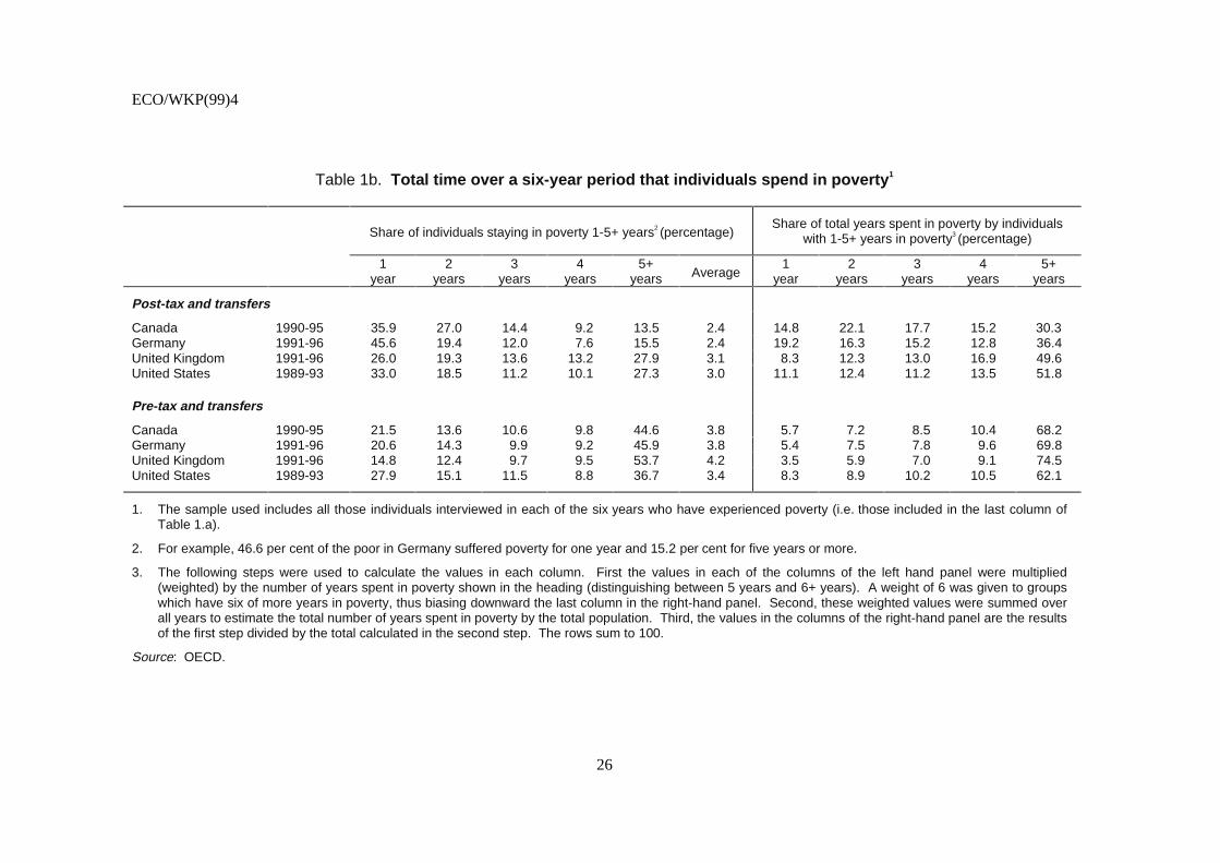
ECO/WKP(99)4

26

Table 1b. Total time over a six-year period that individuals spend in poverty1

Share of individuals staying in poverty 1-5+ years2 (percentage)Share of total years spent in poverty by individuals

with 1-5+ years in poverty3 (percentage)

1year

2years

3years

4years

5+years Average

1year

2years

3years

4years

5+years


Canada 1990-95 35.9 27.0 14.4 9.2 13.5 2.4 14.8 22.1 17.7 15.2 30.3Germany 1991-96 45.6 19.4 12.0 7.6 15.5 2.4 19.2 16.3 15.2 12.8 36.4United Kingdom 1991-96 26.0 19.3 13.6 13.2 27.9 3.1 8.3 12.3 13.0 16.9 49.6United States 1989-93 33.0 18.5 11.2 10.1 27.3 3.0 11.1 12.4 11.2 13.5 51.8


Canada 1990-95 21.5 13.6 10.6 9.8 44.6 3.8 5.7 7.2 8.5 10.4 68.2Germany 1991-96 20.6 14.3 9.9 9.2 45.9 3.8 5.4 7.5 7.8 9.6 69.8United Kingdom 1991-96 14.8 12.4 9.7 9.5 53.7 4.2 3.5 5.9 7.0 9.1 74.5United States 1989-93 27.9 15.1 11.5 8.8 36.7 3.4 8.3 8.9 10.2 10.5 62.1

1. The sample used includes all those individuals interviewed in each of the six years who have experienced poverty (i.e. those included in the last column ofTable 1.a).

2. For example, 46.6 per cent of the poor in Germany suffered poverty for one year and 15.2 per cent for five years or more.

3. The following steps were used to calculate the values in each column. First the values in each of the columns of the left hand panel were multiplied(weighted) by the number of years spent in poverty shown in the heading (distinguishing between 5 years and 6+ years). A weight of 6 was given to groupswhich have six of more years in poverty, thus biasing downward the last column in the right-hand panel. Second, these weighted values were summed overall years to estimate the total number of years spent in poverty by the total population. Third, the values in the columns of the right-hand panel are the resultsof the first step divided by the total calculated in the second step. The rows sum to 100.

Source: OECD.

ECO/WKP(99)4

27

Table 2. Dynamics of poverty: empirical probabilities of exit and re-entry conditional on duration1

Empirical exit hazards2

(rate *100)Empirical re-entry hazards3

(rate *100)

1 year 2 years 3 years 4 yearsAverage4

duration 1 year 2 years 3 years 4 yearsAverage4

duration





1. Latest available six-year period. All spells of poverty (or spells out of poverty for those having just left poverty) whose beginning date is observed andthen followed until they end are selected from the sample used in Table 1b. A spell of poverty (or spells of non-poverty in the case of re-entry) may endbecause the individual transits out of poverty (or re-enters poverty) or because the individual does not transit before the period ends. Therefore, thesample includes spells starting at t+1, t+2, t+3 and t+4 (e.g. in the case of Germany (1991-1996), 1992, 1993, 1994 and 1995).

2. This is calculated as the ratio of those individuals observed to leave poverty after 1, 2, 3 or 4 years in poverty over the population at risk at the beginningof the period. For example, of those who are still in poverty after 1 year, 41.3 per cent are observed to leave poverty between 1 and 2 years in Canada.

3. The re-entry hazard is calculated as the ratio of those individuals observed to fall back into poverty after 1, 2, 3 or 4 years above the poverty line over thepopulation at risk. For example, of those who left poverty and are still above the poverty line after 1 year, 9.7 per cent will fall back into poverty in Canadabetween 1 and 2 years.

4. The average length of the lag is calculated by weighting the probability by the spell length and summing.

Source: OECD.

ECO/WKP(99)4

28

Table 3. Characteristics of the non-poor, shorter-term poor and longer-term poor

Per cent share of persons with a specified characteristic in each group

Household characteristics Total population1 Non-poor1 Poor 1 year2 Always poor1

Canada

Head genderHead male 83.7 87.9 70.6 72.4Head female 16.3 12.1 29.4 27.6

100.0 100.0 100.0 100.0Work attachmentNo worker 18.3 13.6 45.3 36.4One worker 31.2 27.9 42.3 43.9Two workers 39.0 44.3 11.3 17.9More than two workers 11.5 14.2 1.1 1.8

100.0 100.0 100.0 100.0Family type3

Single adult, no children 19.4 16.1 34.3 24.9Two adults, no children 30.1 32.4 15.5 26.7Single adult, children 4.4 2.1 11.3 11.6Two adults, children 31.5 32.4 33.2 29.2Large families 14.6 16.9 5.7 7.6

100.0 100.0 100.0 100.0Age of household headYoung-age head 28.3 25.0 38.2 28.6Prime-age head 34.0 35.7 34.8 33.4Older-working-age head 21.8 22.6 21.6 22.0Retirement-age head 15.9 16.7 5.4 16.0

100.0 100.0 100.0 100.0Education level4

Low education .. .. .. ..Middle education .. .. .. ..Higher education .. .. .. ..

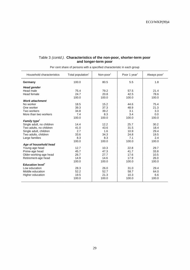
ECO/WKP(99)4

29

Table 3 (contd.). Characteristics of the non-poor, shorter-term poorand longer-term poor



Germany 100.0 80.5 5.5 1.8



100.0 100.0 100.0 100.0Family type3



100.0 100.0 100.0 100.0Education level4

Low education 28.3 26.0 31.0 29.4Middle education 52.2 52.7 58.7 64.0Higher education 19.5 21.3 10.3 6.6

100.0 100.0 100.0 100.0

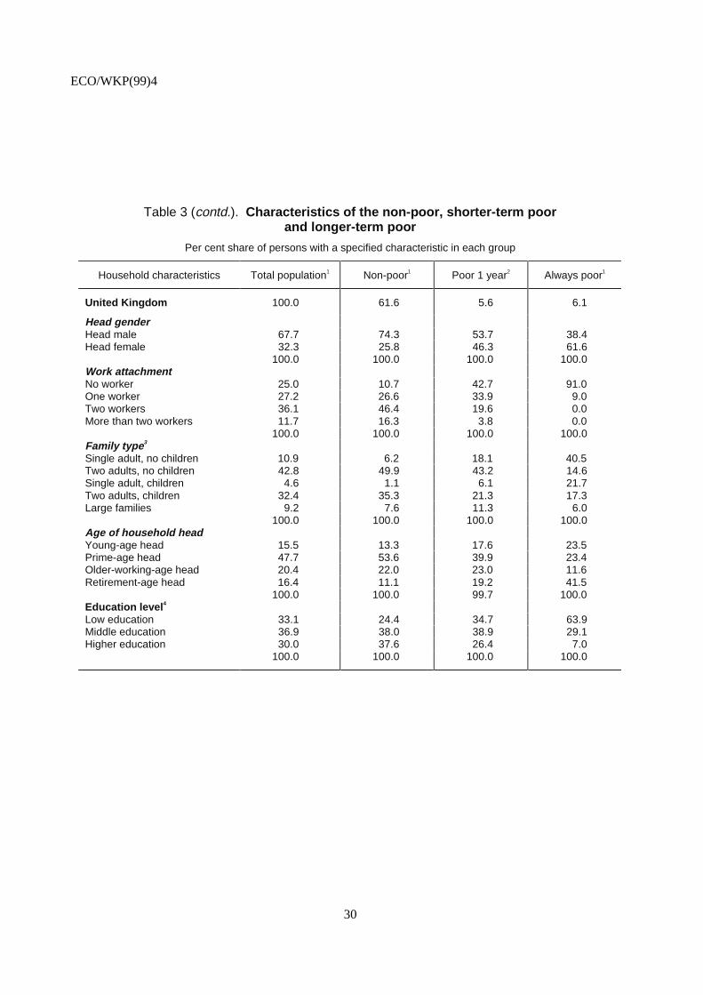
ECO/WKP(99)4

30




United Kingdom 100.0 61.6 5.6 6.1



100.0 100.0 100.0 100.0Family type3



100.0 100.0 99.7 100.0Education level4


100.0 100.0 100.0 100.0

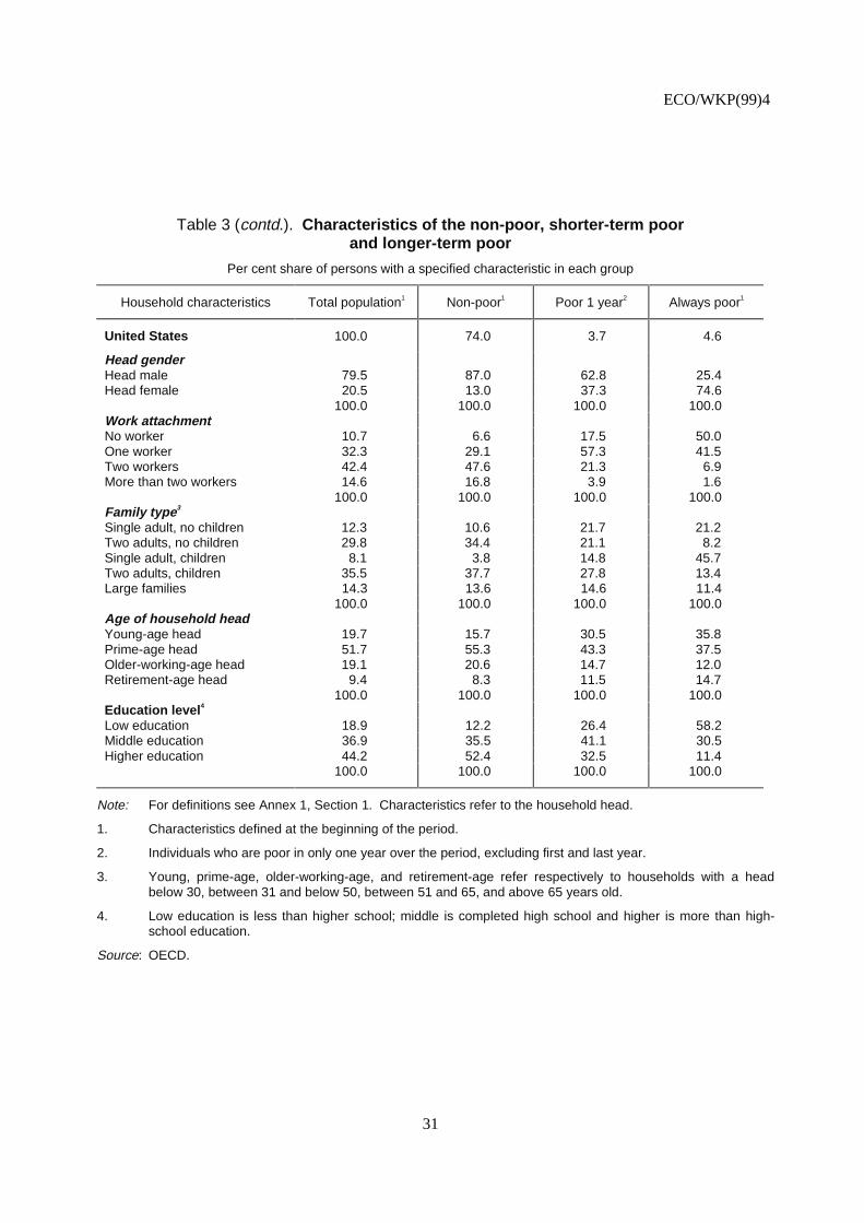
ECO/WKP(99)4

31




United States 100.0 74.0 3.7 4.6



100.0 100.0 100.0 100.0Family type3



100.0 100.0 100.0 100.0Education level4


100.0 100.0 100.0 100.0

Note: For definitions see Annex 1, Section 1. Characteristics refer to the household head.

1. Characteristics defined at the beginning of the period.

2. Individuals who are poor in only one year over the period, excluding first and last year.

3. Young, prime-age, older-working-age, and retirement-age refer respectively to households with a headbelow 30, between 31 and below 50, between 51 and 65, and above 65 years old.

4. Low education is less than higher school; middle is completed high school and higher is more than high-school education.

Source: OECD.

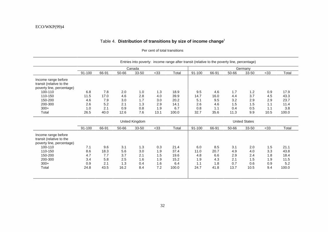
ECO/WKP(99)4

32

Table 4. Distribution of transitions by size of income change1

Per cent of total transitions

Entries into poverty: income range after transit (relative to the poverty line, percentage)

Canada Germany91-100 66-91 50-66 33-50 <33 Total 91-100 66-91 50-66 33-50 <33 Total

Income range beforetransit (relative to thepoverty line, percentage)

100-110 6.8 7.8 2.0 1.0 1.3 18.9 9.5 4.6 1.7 1.2 0.9 17.9110-150 11.5 17.0 4.6 2.8 4.0 39.9 14.7 16.0 4.4 3.7 4.5 43.3150-200 4.6 7.9 3.0 1.7 3.0 20.2 5.1 9.5 3.2 2.9 2.9 23.7200-300 2.6 5.2 2.1 1.3 2.9 14.1 2.6 4.6 1.5 1.5 1.1 11.4300+ 1.0 2.1 0.9 0.8 1.9 6.7 0.8 1.1 0.4 0.5 1.1 3.8Total 26.5 40.0 12.6 7.6 13.1 100.0 32.7 35.6 11.3 9.9 10.5 100.0

United Kingdom United States

91-100 66-91 50-66 33-50 <33 Total 91-100 66-91 50-66 33-50 <33 Total


100-110 7.1 9.6 3.1 1.3 0.3 21.4 6.0 8.5 3.1 2.0 1.5 21.1110-150 8.6 18.3 5.6 3.0 1.9 37.4 11.0 20.7 4.9 4.0 3.3 43.8150-200 4.7 7.7 3.7 2.1 1.5 19.6 4.8 6.6 2.9 2.4 1.8 18.4200-300 3.4 5.8 2.5 1.6 1.9 15.2 1.9 4.3 2.1 1.5 1.9 11.5300+ 0.9 2.1 1.3 0.4 1.6 6.4 1.1 1.8 0.7 0.6 0.9 5.2Total 24.8 43.5 16.2 8.4 7.2 100.0 24.7 41.8 13.7 10.5 9.4 100.0

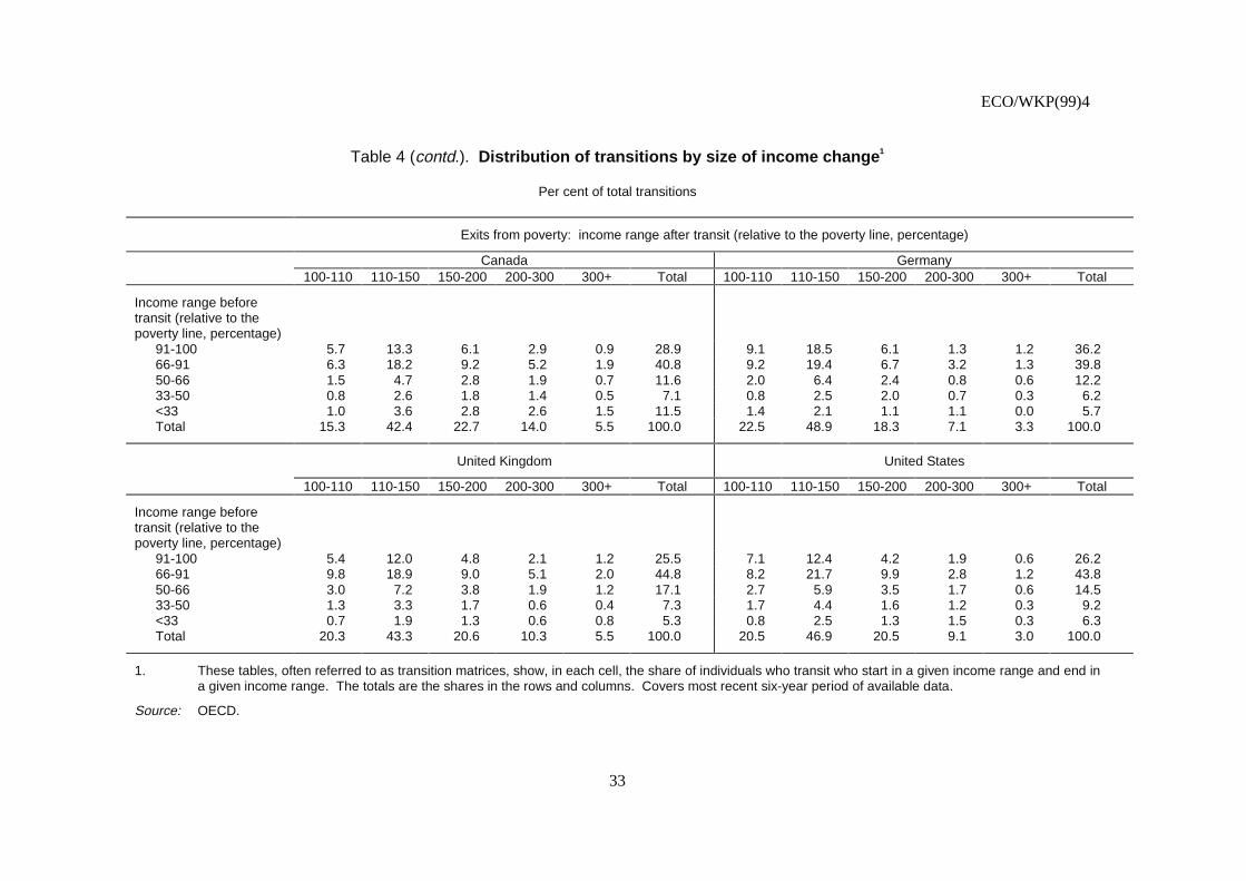
ECO/WKP(99)4

33

Table 4 (contd.). Distribution of transitions by size of income change1

Per cent of total transitions

Exits from poverty: income range after transit (relative to the poverty line, percentage)

Canada Germany100-110 110-150 150-200 200-300 300+ Total 100-110 110-150 150-200 200-300 300+ Total


91-100 5.7 13.3 6.1 2.9 0.9 28.9 9.1 18.5 6.1 1.3 1.2 36.266-91 6.3 18.2 9.2 5.2 1.9 40.8 9.2 19.4 6.7 3.2 1.3 39.850-66 1.5 4.7 2.8 1.9 0.7 11.6 2.0 6.4 2.4 0.8 0.6 12.233-50 0.8 2.6 1.8 1.4 0.5 7.1 0.8 2.5 2.0 0.7 0.3 6.2<33 1.0 3.6 2.8 2.6 1.5 11.5 1.4 2.1 1.1 1.1 0.0 5.7Total 15.3 42.4 22.7 14.0 5.5 100.0 22.5 48.9 18.3 7.1 3.3 100.0

United Kingdom United States

100-110 110-150 150-200 200-300 300+ Total 100-110 110-150 150-200 200-300 300+ Total


91-100 5.4 12.0 4.8 2.1 1.2 25.5 7.1 12.4 4.2 1.9 0.6 26.266-91 9.8 18.9 9.0 5.1 2.0 44.8 8.2 21.7 9.9 2.8 1.2 43.850-66 3.0 7.2 3.8 1.9 1.2 17.1 2.7 5.9 3.5 1.7 0.6 14.533-50 1.3 3.3 1.7 0.6 0.4 7.3 1.7 4.4 1.6 1.2 0.3 9.2<33 0.7 1.9 1.3 0.6 0.8 5.3 0.8 2.5 1.3 1.5 0.3 6.3Total 20.3 43.3 20.6 10.3 5.5 100.0 20.5 46.9 20.5 9.1 3.0 100.0

1. These tables, often referred to as transition matrices, show, in each cell, the share of individuals who transit who start in a given income range and end ina given income range. The totals are the shares in the rows and columns. Covers most recent six-year period of available data.

Source: OECD.

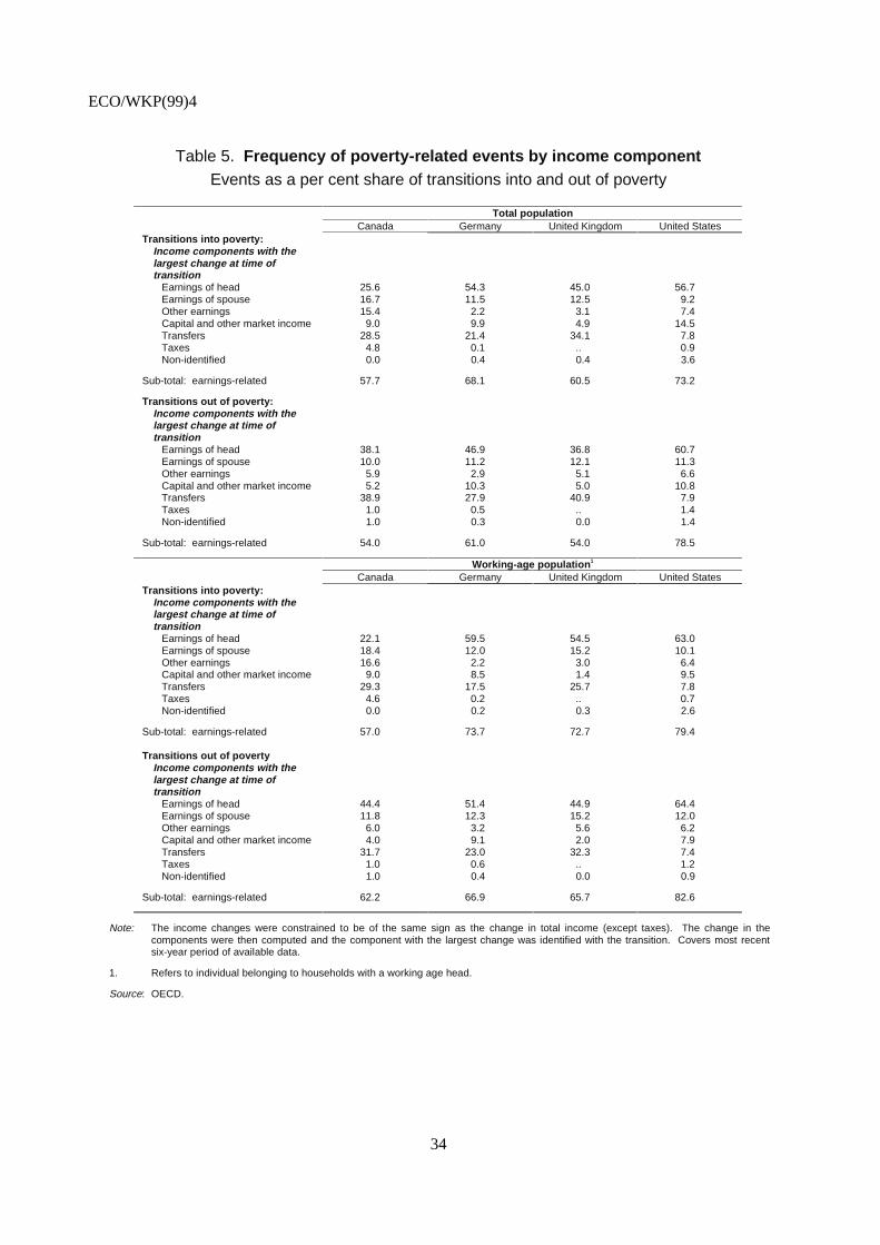
ECO/WKP(99)4

34

Table 5. Frequency of poverty-related events by income componentEvents as a per cent share of transitions into and out of poverty

Total populationCanada Germany United Kingdom United States

Transitions into poverty:Income components with thelargest change at time oftransition

Earnings of head 25.6 54.3 45.0 56.7Earnings of spouse 16.7 11.5 12.5 9.2Other earnings 15.4 2.2 3.1 7.4Capital and other market income 9.0 9.9 4.9 14.5Transfers 28.5 21.4 34.1 7.8Taxes 4.8 0.1 .. 0.9Non-identified 0.0 0.4 0.4 3.6

Sub-total: earnings-related 57.7 68.1 60.5 73.2

Transitions out of poverty:Income components with thelargest change at time oftransition



Working-age population1

Canada Germany United Kingdom United StatesTransitions into poverty:

Income components with thelargest change at time oftransition



Transitions out of povertyIncome components with thelargest change at time oftransition



Note: The income changes were constrained to be of the same sign as the change in total income (except taxes). The change in thecomponents were then computed and the component with the largest change was identified with the transition. Covers most recentsix-year period of available data.

1. Refers to individual belonging to households with a working age head.

Source: OECD.

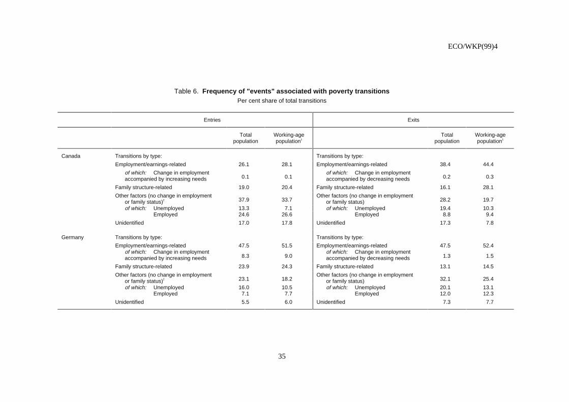
ECO/WKP(99)4

35

Table 6. Frequency of "events" associated with poverty transitionsPer cent share of total transitions

Entries Exits

Totalpopulation

Working-agepopulation1

Totalpopulation


Canada Transitions by type: Transitions by type:

Employment/earnings-related 26.1 28.1 Employment/earnings-related 38.4 44.4

of which: Change in employmentaccompanied by increasing needs 0.1 0.1

of which: Change in employmentaccompanied by decreasing needs 0.2 0.3

Family structure-related 19.0 20.4 Family structure-related 16.1 28.1

Other factors (no change in employmentor family status)2 37.9 33.7

Other factors (no change in employmentor family status) 28.2 19.7

of which: Unemployed 13.3 7.1 of which: Unemployed 19.4 10.3Employed 24.6 26.6 Employed 8.8 9.4

Unidentified 17.0 17.8 Unidentified 17.3 7.8

Germany Transitions by type: Transitions by type:

Employment/earnings-related 47.5 51.5 Employment/earnings-related 47.5 52.4of which: Change in employmentaccompanied by increasing needs 8.3 9.0



Other factors (no change in employmentor family status)2 23.1 18.2




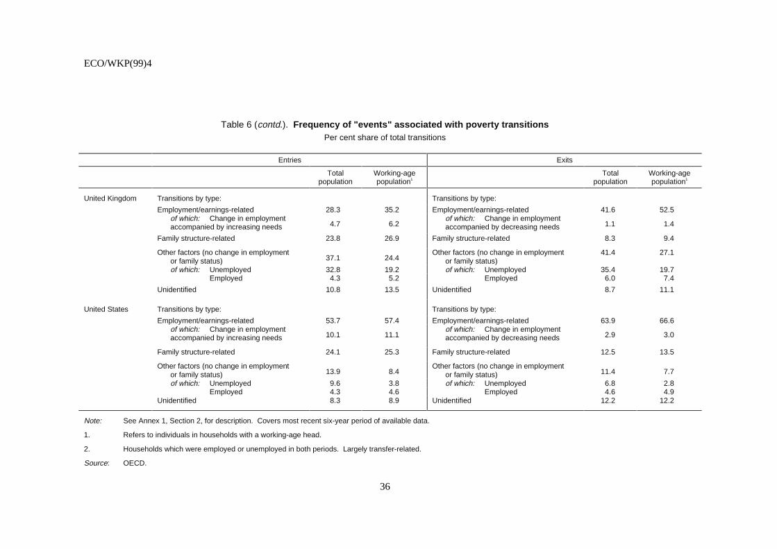
ECO/WKP(99)4

36

Table 6 (contd.). Frequency of "events" associated with poverty transitionsPer cent share of total transitions

Entries Exits

Totalpopulation


Totalpopulation


United Kingdom Transitions by type: Transitions by type:





Other factors (no change in employmentor family status)

41.4 27.1



United States Transitions by type: Transitions by type:








Note: See Annex 1, Section 2, for description. Covers most recent six-year period of available data.

1. Refers to individuals in households with a working-age head.

2. Households which were employed or unemployed in both periods. Largely transfer-related.

Source: OECD.

ECO/WKP(99)4

37

Table 7. Frequency of "events" associated with poverty transitions: by family type1,2

Per cent share of total transitions

EntriesSingle adult,

no child2 adults,

no childrenSingle adult,

children2 adults,children

Canada Share of family type in total sample 17.9 42.0 3.4 36.7Share of family type in total transitions 23.3 28.5 11.8 36.5

Transitions which were:

Employment/earnings-related 20.4 31.7 13.3 34.9of which: Change in employmentaccompanied by increasing needs .. 0.0 0.0 0.3

Family structure-related 30.0 14.5 54.6 7.5

Other factors (no change in employmentor family status)2 44.8 34.4 20.1 29.7

of which: Unemployed 12.6 9.1 7.8 0.6Employed 32.2 25.3 12.3 29.1

Unidentified 4.8 19.4 12.0 27.9

Germany Share of family type in total sample 8.8 38.4 2.3 50.4Share of family type in total transitions 18.5 25.3 11.2 45.0






Unidentified 2.8 5.6 3.3 7.8

United Kingdom Share of family type in total sample 10.4 40.6 4.3 44.7Share of family type in total transitions 23.6 27.3 12.8 36.4




Other factors (no change in employmentor family status) 31.2 29.5 16.0 20.5



United States Share of family type in total sample 9.5 24.7 10.1 55.7Share of family type in total transitions 16.4 17.1 21.1 45.3







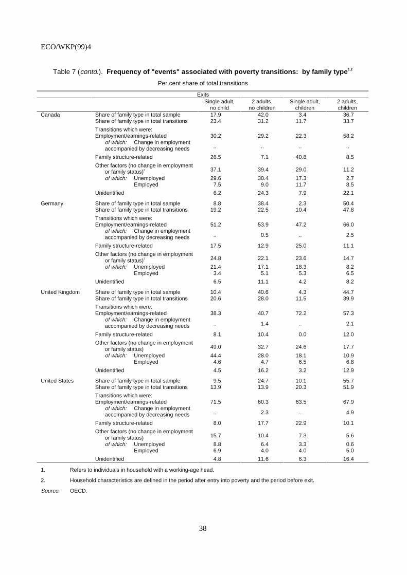
ECO/WKP(99)4

38

Table 7 (contd.). Frequency of "events" associated with poverty transitions: by family type1,2

Per cent share of total transitions

ExitsSingle adult,

no child2 adults,

no childrenSingle adult,

children2 adults,children

Canada Share of family type in total sample 17.9 42.0 3.4 36.7Share of family type in total transitions 23.4 31.2 11.7 33.7

Transitions which were:Employment/earnings-related 30.2 29.2 22.3 58.2

of which: Change in employmentaccompanied by decreasing needs .. .. .. ..





Germany Share of family type in total sample 8.8 38.4 2.3 50.4Share of family type in total transitions 19.2 22.5 10.4 47.8


of which: Change in employmentaccompanied by decreasing needs .. 0.5 .. 2.5





United Kingdom Share of family type in total sample 10.4 40.6 4.3 44.7Share of family type in total transitions 20.6 28.0 11.5 39.9







United States Share of family type in total sample 9.5 24.7 10.1 55.7Share of family type in total transitions 13.9 13.9 20.3 51.9







1. Refers to individuals in household with a working-age head.

2. Household characteristics are defined in the period after entry into poverty and the period before exit.

Source: OECD.

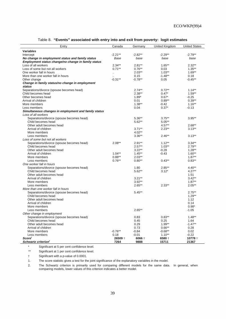
ECO/WKP(99)4

39

Table 8. “Events” associated with entry into and exit from poverty: logit estimates

Entry Canada Germany United Kingdom United States

VariablesIntercept -2.21** -2.82** -2.29** -2.79**No change in employment status and family status Base base base baseEmployment status change/no change in family statusLoss of all workers 2.34** 2.81** 1.65** 2.32**Loss of some but not all workers 0.71** 0.76** 0.03 1.35**One worker fall in hours .. 2.03** 1.03** 1.69**More than one worker fall in hours .. 0.15 -1.48** 0.18Other change -0.31** -0.78** 0.05 -0.45**Change in family status/no change in employmentstatusSeparations/divorce (spouse becomes head) 2.74** 0.72** 1.14**Child becomes head 2.38** 0.47* 1.59**Other becomes head 1.89* 0.67* -0.25Arrival of children 0.01 0.89** 0.39**More members 1.38** -0.42 1.16**Less members 0.04 0.37* -0.13Simultaneous changes in employment and family statusLoss of all workers

Separations/divorce (spouse becomes head) 5.36** 3.75** 3.95**Child becomes head 5.62** 5.05**Other adult becomes head 4.57** 2.68**Arrival of children 3.71** 2.23** 3.13**More members 4.02**Less members 3.36** 2.46** 3.13**

Loss of some but not all workersSeparations/divorce (spouse becomes head) 2.08** 2.91** 1.12** 3.34**Child becomes head 2.57** 1.03** 2.79**Other adult becomes head 3.22** -0.28 1.28**Arrival of children 1.04** 1.45** -0.43 1.60**More members 0.88** 2.03** 1.87**Less members 0.76** 0.80** 0.43** 0.83**

One worker fall in hoursSeparations/divorce (spouse becomes head) 1.80 2.85** 4.40**Child becomes head 5.62** 3.12* 4.27**Other adult becomes head 1.51Arrival of children 3.21** 3.42**More members 3.92** 1.87**Less members 2.65** 2.33** 2.05**

More than one worker fall in hoursSeparations/divorce (spouse becomes head) 5.45** 2.75**Child becomes head 1.29**Other adult becomes head 1.12Arrival of children 0.14More members 0.98*Less members 2.65** -1.05

Other change in employmentSeparations/divorce (spouse becomes head) 0.83 0.83** 1.48**Child becomes head 0.45 0.25 1.64Other adult becomes head 0.29 1.99** -1.47**Arrival of children 0.73 0.66** 0.28More members -0.76** -0.84 -0.68** 0.02Less members 0.18 -0.01 1.10** -0.22

Score1 26509 † 6066 † 6580 † 10778 †Schwartz criterion2 7264 9888 15711 21367

* Significant at 5 per cent confidence level.

** Significant at 1 per cent confidence level.

† Significant with a p-value of 0.0001.

1. The score statistic gives a test for the joint significance of the explanatory variables in the model.

2. The Schwartz criterion is primarily used for comparing different models for the same data. In general, whencomparing models, lower values of this criterion indicates a better model.

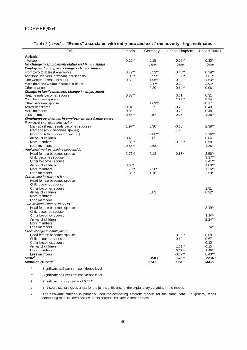
ECO/WKP(99)4

40

Table 8 (contd.). “Events” associated with entry into and exit from poverty: logit estimates

Exit Canada Germany United Kingdom United States

VariablesIntercept -0.15** 0.15 -0.25** -0.80**No change in employment status and family status base base baseEmployment change/no change in family statusFrom zero to at least one worker 0.72** 0.53** 0.45** 0.39**Additional workers in working households 1.05** 0.99** 1.12** 1.61**One worker increase in hours -0.39 1.96** 0.12 1.53**More than one worker increase in hours -0.47** 0.33 2.01**Other change -0.20 0.64** -0.06Change in family status/no change in employmentHead female becomes spouse 0.83** 0.01 0.31Child becomes spouse 1.29** 0.94Other becomes spouse 1.69** -0.17Arrival of children -0.04 0.25 -0.26 -0.40More members 0.33* 0.28 -0.48Less members 0.53** 0.57 0.75 1.36**Simultaneous changes in employment and family statusFrom zero to at least one worker

Marriage (head female becomes spouse) 1.97** 0.30 -0.28 2.38**Marriage (child becomes spouse) 1.43Marriage (other becomes spouse) 2.00** 2.16**Arrival of children 0.43 0.05 0.84More members 1.82** 3.92** 0.58Less members 0.88** 0.63 1.28*

Additional work in working householdsHead female becomes spouse 2.72** -0.13 0.88* 3.56**Child becomes spouse 3.37**Other becomes spouse 2.41**Arrival of children 0.68* 1.89**More members 1.73** 2.38* 1.36**Less members 1.38** -1.18 2.59**

One worker increase in hoursHead female becomes spouseChild becomes spouseOther becomes spouse 1.81Arrival of children 0.83 0.92*More membersLess members

Two workers increase in hoursHead female becomes spouse 3.49**Child becomes spouseOther becomes spouse 3.24**Arrival of children 2.24**More membersLess members 2.74**

Other change in employmentHead female becomes spouse 0.95** 0.68Child becomes spouse 0.62 0.67Other becomes spouse -0.10Arrival of children 1.09** -0.13More members 0.07* 2.45**Less members -0.07** 0.43**

Score1 358 † 572 † 2234 †Schwartz criterion2 3737 9983 13335





2. The Schwartz criterion is primarily used for comparing different models for the same data. In general, whencomparing models, lower values of this criterion indicates a better model.

ECO/WKP(99)4

41

Table 9. Estimates of exit rates from poverty by length of time spent in poverty1

Canada, 1986-1995 Germany, 1984-1996 United Kingdom, 1991-1996 United States, 1980-1993

Length of timeabove the poverty

line

Probability ofexiting poverty

Share of thoseremaining in

poverty



poverty



poverty



poverty

1 year 0.50 0.50 0.50 0.50 0.36 0.64 0.41 0.592 years 0.45 0.27 0.42 0.29 0.25 0.48 0.34 0.393 years 0.40 0.17 0.35 0.19 0.17 0.40 0.28 0.284 years 0.35 0.11 0.28 0.13 0.11 0.36 0.22 0.225 years 0.30 0.07 0.22 0.10 0.07 0.33 0.18 0.186 years 0.26 0.06 0.17 0.09 0.14 0.167 years 0.22 0.04 0.13 0.08 0.11 0.148 years 0.19 0.03 0.10 0.07 0.08 0.139 years 0.07 0.06 0.06 0.1210 years 0.05 0.06 0.05 0.12

1. These estimates represent the probability of leaving a poverty spell conditional on the length of time already spent in poverty (see Annex 1, Section 3).These results correspond to an average prime-age individual, with high-school level of education (with no disabilities or health problems).

ECO/WKP(99)4

42

Table 10. Percentage of people remaining in poverty1

No-one employed Head employedHead and some other family member

employed1 or more

years4 or more

years10 or more

years1 or more

years4 or more

years10 or more

years1 or more

years4 or more

years10 or more

years

Canada

Reference person2 54.7 14.6 4.3 48.4 9.6 2.1 43.2 6.6 1.0Alternative characteristicsOld age person (65+) 41.5 5.7 0.8 35.5 3.3 0.3 30.9 2.0 0.1Two or more adults households withchildren

57.4 17.2 5.7 51.1 11.7 2.9 45.9 8.1 1.5

Germany

Reference person2 55.5 19.0 10.1 38.6 6.1 1.8 27.8 2.1 0.3Alternative characteristicsSingle parent households 64.4 29.4 18.8 47.6 11.8 5.0 35.8 4.8 1.3Previous poverty experience 61.1 25.2 15.1 44.1 9.3 3.5 32.6 3.5 0.8High growth scenario (GDP growthrate = 3 per cent)

51.8 15.9 7.9 36.7 5.2 1.4 26.3 1.7 0.2

United Kingdom

Reference person2 60.7 31.3 42.4 12.3 29.0 4.1Alternative characteristicsSingle parent households 64.5 36.3 46.4 15.6 32.3 5.7Previous Poverty experience 68.7 42.4 51.1 20.2 36.7 8.2

United States

Reference person2 58.1 20.7 10.4 52.9 15.5 6.7 44.4 8.9 2.8Alternative characteristicsLow educational attainment 62.6 25.9 14.6High educational attainment 47.2 10.8 3.9Non-white 64.4 28.3 16.6Non-white with low education 68.6 34.1 21.9

Single parent households 62.7 26.1 14.7 57.6 20.2 10.1Previous Poverty experience 63.0 26.5 15.0 58.0 20.5 10.3 49.5 12.5 4.9High growth scenario (GDP growthrate=3 per cent)

56.7 19.2 9.3 43.0 8.0 2.4

The worst hit person3 76.4 47.0 34.6 72.5 40.2 27.7

1. Calculations based on the logit estimates of a duration model of the time spent in single poverty spells by individuals who fall into poverty (see Annex 1, Section 3). Taking the value in the fourth row,third column as an example, the percentage of people who are still in poverty after ten years is 10.1 in Germany, the reference person when no-one is employed in the household.

2. The reference person is a prime-age male, with high-school level of education, who is head of household, single, with no dependent children and not working at the time of falling into poverty.3. Belonging to a female-headed, single-parent household, non-white with low education and previous poverty spells.

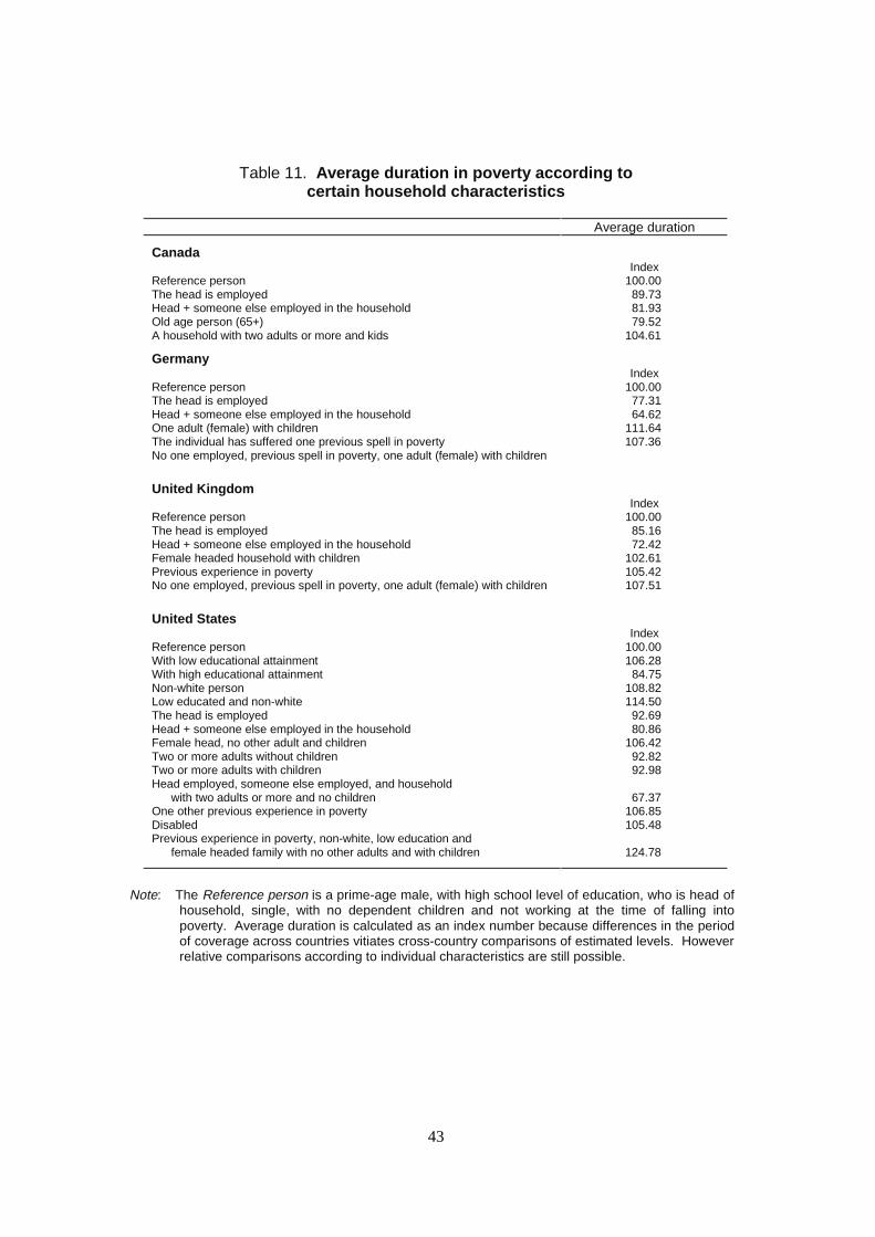
43

Table 11. Average duration in poverty according tocertain household characteristics

Average duration

CanadaIndex

Reference person 100.00The head is employed 89.73Head + someone else employed in the household 81.93Old age person (65+) 79.52A household with two adults or more and kids 104.61

GermanyIndex

Reference person 100.00The head is employed 77.31Head + someone else employed in the household 64.62One adult (female) with children 111.64The individual has suffered one previous spell in poverty 107.36No one employed, previous spell in poverty, one adult (female) with children

United KingdomIndex

Reference person 100.00The head is employed 85.16Head + someone else employed in the household 72.42Female headed household with children 102.61Previous experience in poverty 105.42No one employed, previous spell in poverty, one adult (female) with children 107.51

United StatesIndex

Reference person 100.00With low educational attainment 106.28With high educational attainment 84.75Non-white person 108.82Low educated and non-white 114.50The head is employed 92.69Head + someone else employed in the household 80.86Female head, no other adult and children 106.42Two or more adults without children 92.82Two or more adults with children 92.98Head employed, someone else employed, and household

with two adults or more and no children 67.37One other previous experience in poverty 106.85Disabled 105.48Previous experience in poverty, non-white, low education and

female headed family with no other adults and with children 124.78

Note: The Reference person is a prime-age male, with high school level of education, who is head ofhousehold, single, with no dependent children and not working at the time of falling intopoverty. Average duration is calculated as an index number because differences in the periodof coverage across countries vitiates cross-country comparisons of estimated levels. Howeverrelative comparisons according to individual characteristics are still possible.

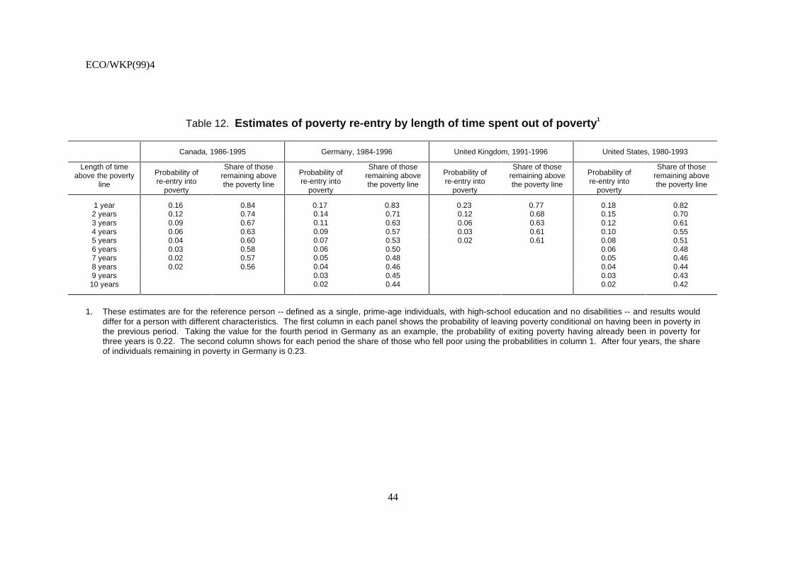
ECO/WKP(99)4

44

Table 12. Estimates of poverty re-entry by length of time spent out of poverty1

Canada, 1986-1995 Germany, 1984-1996 United Kingdom, 1991-1996 United States, 1980-1993

Length of timeabove the poverty

line

Probability ofre-entry into

poverty

Share of thoseremaining abovethe poverty line


poverty



poverty



poverty


1 year 0.16 0.84 0.17 0.83 0.23 0.77 0.18 0.822 years 0.12 0.74 0.14 0.71 0.12 0.68 0.15 0.703 years 0.09 0.67 0.11 0.63 0.06 0.63 0.12 0.614 years 0.06 0.63 0.09 0.57 0.03 0.61 0.10 0.555 years 0.04 0.60 0.07 0.53 0.02 0.61 0.08 0.516 years 0.03 0.58 0.06 0.50 0.06 0.487 years 0.02 0.57 0.05 0.48 0.05 0.468 years 0.02 0.56 0.04 0.46 0.04 0.449 years 0.03 0.45 0.03 0.4310 years 0.02 0.44 0.02 0.42

1. These estimates are for the reference person -- defined as a single, prime-age individuals, with high-school education and no disabilities -- and results woulddiffer for a person with different characteristics. The first column in each panel shows the probability of leaving poverty conditional on having been in poverty inthe previous period. Taking the value for the fourth period in Germany as an example, the probability of exiting poverty having already been in poverty forthree years is 0.22. The second column shows for each period the share of those who fell poor using the probabilities in column 1. After four years, the shareof individuals remaining in poverty in Germany is 0.23.

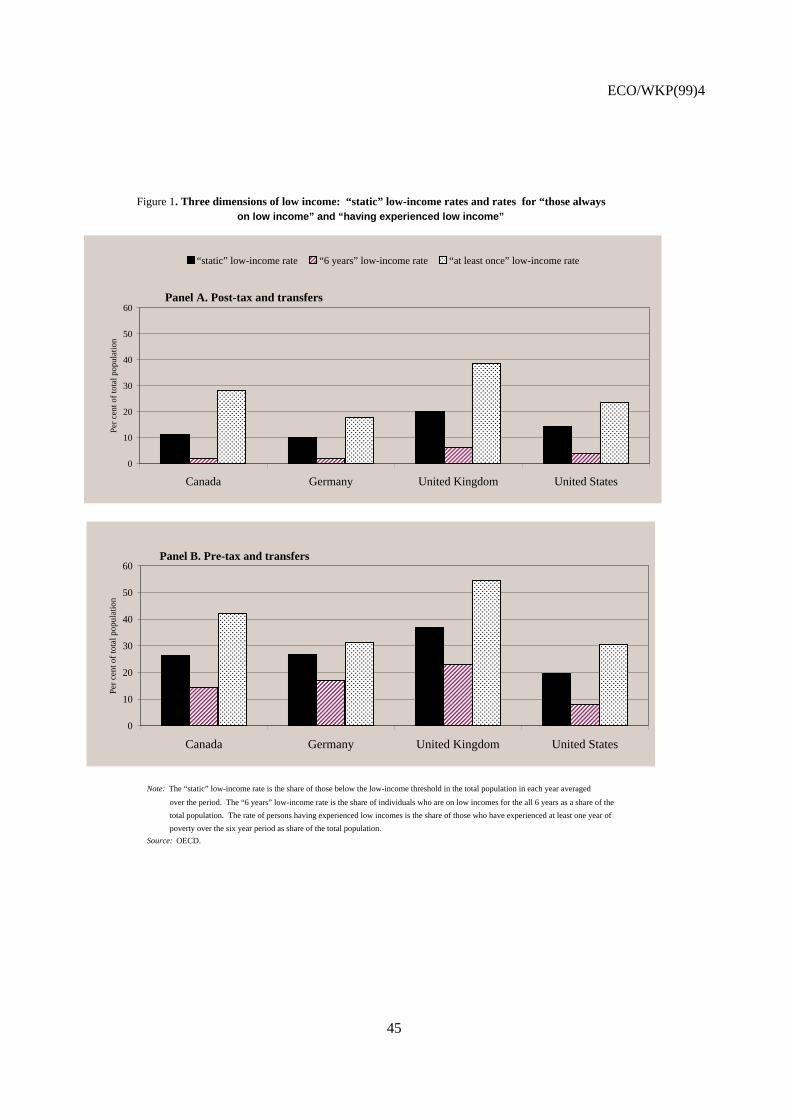
ECO/WKP(99)4

45

Figure 1. Three dimensions of low income: “static” low-income rates and rates for “those alwayson low income” and “having experienced low income”

Note: The “static” low-income rate is the share of those below the low-income threshold in the total population in each year averaged

over the period. The “6 years” low-income rate is the share of individuals who are on low incomes for the all 6 years as a share of the

total population. The rate of persons having experienced low incomes is the share of those who have experienced at least one year of

poverty over the six year period as share of the total population.

Source:OECD.

Panel A. Post-tax and transfers

0

10

20

30

40

50

60

Canada Germany United Kingdom United States

Pe

rce

nto

fto

talp

op

ula

tion

“static” low-income rate “6 years” low-income rate “at least once” low-income rate

Panel B. Pre-tax and transfers

0

10

20

30

40

50

60

Canada Germany United Kingdom United States

Pe

rce

nto

fto

talp

op

ula

tion

ECO/WKP(99)4

46

ANNEX 1: TECHNICAL NOTES

52. This annex contains background information to the main paper. The first section describes thedata sources and issues and provides some supplementary descriptive information from Part 3 of the mainpaper. Sections 2 and 3 explain in greater detail the methodology and the results from Section 4 (povertytransitions) and Section 5 (poverty duration) in the main paper.

1. Data sources and methodology

1.1. Data sources

53. The data used in this study are longitudinal micro-databases containing socio-economicinformation on private households for four countries. This type of data set allows individuals to befollowed over time.

54. The Canadian Longitudinal Administrative Database (LAD): This data file runs from 1982 to1994. This is a large file based on tax records and this information is used to attach family-basedinformation to individuals. Inclusion in the sample requires the individual to have filed tax and the personis excluded if he or she stops filing for tax, and are replaced by other filers. The population coverage of theadult population is high, reflecting the high rate of tax filing. While income variables are generally of highquality (except for non-taxable income transfers before 1992), the amount of additional information ormore detailed information on employment status, hours worked, and individual characteristics(e.g. education) is limited41. In addition to this limited information on individual and householdcharacteristics, it is not possible to trace children over time, for example, as they form new households. Todefine households a concept referred as “census families” was used as oppose to the household concept onsurvey data42.

55. The German Socio-Economic Panel (GSOEP) is a longitudinal data set which containsinformation on around 28 000 individuals, around 16 000 households. The GSOEP in its current version(1997) contains 13 waves, from 1984 to 1996. It covers all Germany since 1991 (only West Germanyfrom 1984 to 1990). The study only makes use of the West German sub-sample.

56. Due to German data protection laws, researchers outside Germany only have access to a 95 percent random sample of the original sample. This study uses the information as provided by the SyracuseUniversity in the GSOEP Equivalent File. The Equivalent File attempts to create a common set ofvariables for Germany and for the Panel Survey of Income Dynamics (PSID) for the United States.

41. These gaps should be filled by the more recent Survey on Labour and Income Dynamics (SLID)

42. This includes “husbands and wives (common law or legally married) with or without their never-marriedchildren, lone parents and their never-married children, with everyone else being a non-family person”.Thus there can be several census families living in the same household – e.g. a divorced daughter with achild living with her parents would be classified a belonging to a separate household.

ECO/WKP(99)4

47

57. The GSOEP provides full information in each wave of the individual characteristics (e.g. sex,age, nationality), family status (e.g. marital status, relationship with respect to the head of the household,household members), human capital variables (e.g. education) and labour-market status, as well as incomeinformation. Data on income in the Equivalent File is based on original information in the GSOEP plus taxsimulation done at Syracuse.

58. The British Household Panel Survey (BHPS) runs from 1991 to 1996 and is a nationallyrepresentative sample of private households in Great Britain. Its current version includes waves one to sixfrom 1991 to 1996. The sample size is about 5 500 households with around 17 000 individuals. The fullsample is used throughout the study. Data for taxes were not available in the data file for all years andpre-tax income was used in this study.

59. The Panel Survey of Income Dynamics (PSID) is a longitudinal survey, starting in 1968, of arepresentative sample of US individuals and the family units in which they reside. The study is conductedat the Survey Research Center, Institute for Social Research, University of Michigan. It emphasises thedynamic aspects of economic and demographic behaviour, but its content is broad, including sociologicaland psychological measures. The data are collected annually, and the data files contain the full span ofinformation collected over the course of the study. This study uses the PSID Equivalent file, as providedby the University of Syracuse, which is an attempt to create a homogeneous set of variables, in particular,income variables for Germany and the United States. This file only includes the PSID waves from 1980to 1993. The sample size used is of around 33 000 individuals grouped in around 7 800 households.

60. The sample for sections three and four of the study uses only the last six waves available of eachlongitudinal data set. That is, from 1991 to 1996 for the BHPS and GSOEP Equivalent File; from 1990 to1995 for the LAD; and from 1988 to 1993 for the PSID Equivalent File. The sample in Section 5 includesall information available. It includes all the West German sub-sample from 1984 to 1996, the LAD samplefrom 1985 to 1995, the BHPS from 1991 to 1996 and the PSID Equivalent File from 1980 to 1993.

61. Table 1a uses the information in each of the last six waves, while Table 1b uses a sub-sample ofall those individuals interviewed in each of the last six waves. Data in Table 2 is further restricted toinclude only those spells of poverty whose beginning period can be observed over the last six years orwaves. Tables 3 to 7 use a sample consisting of all individuals who transit into or out of poverty betweentwo consecutive years of the sample among all individuals interviewed in each of the last six years, butexcluding those individuals who were poor in the first year. Tables corresponding to Section 5 use asample of all poverty spells of individuals which began between 1984 and 1996 in the West Germansub-sample of the GSOEP; between 1991 and 1996 for the BHPS; between 1985 and 1995 for the LAD;and between 1980 and 1993 for the PSID.

62. Where appropriate, the samples were weighted to make them representative of the wholepopulation.

1.2. Defining poverty thresholds

63. The household unity and the income and concept employ the same definitions used in Burniauxet al. (1998) Annex 1 using an equivalence scale elasticity of 0.5. The poverty threshold is defined as50 per cent of median income.

1.3. Characteristics of the non-poor, shorter-term poor and longer-term poor (Table 3)

64. Two tables are presented as background to Table 3: one for the total population (a cut-downversion of this is shown in Table 3 of the main text) and for individuals living in households with a

ECO/WKP(99)4

48

working-age head (referred to below as the “working-age” population (see Table A2 ). Each table presentsinformation for three groups depending on the poverty experience over the six-year period. These can bedefined in terms of a sequence of N’s (not poor) and P’s (poor):

− The longer-term poor: those poor throughout the period – i.e. with a sequence PPPPPP. Thisgroup also includes those poor for six or more years.

− Those never poor: all individuals with a sequence NNNNNN.

− The short-term poor: those only poor once in the six-year period where the beginning and theend of the spell is observed, i.e. individuals with the sequences NPNNNN, NNPNNN,NNNPNN, NNNNPN.

65. Individuals in each of these three groups were then decomposed by the characteristics of thehouseholds in which they live: sex of the household head; employment status (no worker; one worker;two workers and more than two workers); family type (single-adult households with and without childrenand two or more adult households with and without children); age of the household head broken down intofour groups (young heads: 18 to 30 years old; prime-age heads: 31 to 50; older working-age heads: 51to 65 and retirement-age heads: above 65 years of age); education of the household head (lowereducation: individuals in households where the head has less than high-school leaving certificate; middle:with high-school leaving certificate; and, higher: is more than secondary leaving certificate).

66. The degree of concentration of particular characteristics among the longer-term or shorter-termpoor is indicated by comparing the shares (by characteristic) for these two groups with the share (for thesame characteristic) at the level of the total population and of the non-poor.

67. Results can depend on the year in which the characteristics are defined for the total population,the “non-poor” and the “always” poor particularly for the breakdown by age which ages over the period.For this reason, the results in Table A1 are also defined at the beginning and end of the period. The resultsbroadly hold whichever period is used.

68. A comparison between the total population and “working-age” population in Table A.1. showsthat the retirement-age households (which are concentrated in single and two adult households withoutchildren) are more concentrated among longer-term poor. Take, as an example, single-adult householdswith no children for the United States. For the total population (left-hand panel) characteristics at thebeginning of the period, the share of this group in the long-term poor is 53.3 per cent compared with13.2 per cent for the non-poor. For the “working-age” population (right-hand panel characteristics definedat the beginning of the period), the share of this group in the long-term poor drops to 11.4 per centcompared with a share of 12.1 for the non-poor. This difference is less marked for the United Kingdom.

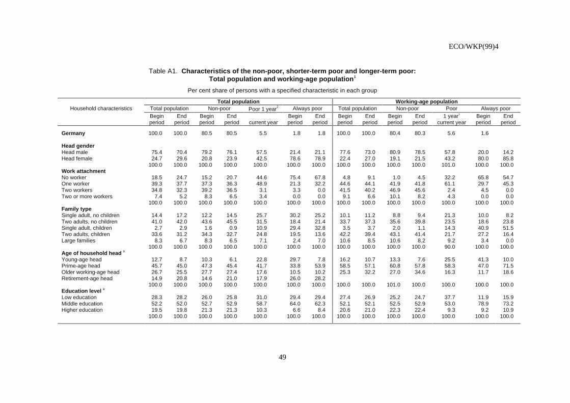
ECO/WKP(99)4

49

Table A1. Characteristics of the non-poor, shorter-term poor and longer-term poor:Total population and working-age population1


Total population Working-age populationHousehold characteristics Total population Non-poor Poor 1 year2 Always poor Total population Non-poor Poor Always poor

Beginperiod

Endperiod

Beginperiod

Endperiod current year

Beginperiod

Endperiod

Beginperiod

Endperiod

Beginperiod

Endperiod

1 year1

current yearBeginperiod

Endperiod

Germany 100.0 100.0 80.5 80.5 5.5 1.8 1.8 100.0 100.0 80.4 80.3 5.6 1.6

Head genderHead male 75.4 70.4 79.2 76.1 57.5 21.4 21.1 77.6 73.0 80.9 78.5 57.8 20.0 14.2Head female 24.7 29.6 20.8 23.9 42.5 78.6 78.9 22.4 27.0 19.1 21.5 43.2 80.0 85.8

100.0 100.0 100.0 100.0 100.0 100.0 100.0 100.0 100.0 100.0 100.0 101.0 100.0 100.0Work attachmentNo worker 18.5 24.7 15.2 20.7 44.6 75.4 67.8 4.8 9.1 1.0 4.5 32.2 65.8 54.7One worker 39.3 37.7 37.3 36.3 48.9 21.3 32.2 44.6 44.1 41.9 41.8 61.1 29.7 45.3Two workers 34.8 32.3 39.2 36.5 3.1 3.3 0.0 41.5 40.2 46.9 45.6 2.4 4.5 0.0Two or more workers 7.4 5.2 8.3 6.5 3.4 0.0 0.0 9.1 6.6 10.1 8.2 4.3 0.0 0.0

100.0 100.0 100.0 100.0 100.0 100.0 100.0 100.0 100.0 100.0 100.0 100.0 100.0 100.0Family typeSingle adult, no children 14.4 17.2 12.2 14.5 25.7 30.2 25.2 10.1 11.2 8.8 9.4 21.3 10.0 8.2Two adults, no children 41.0 42.0 43.6 45.5 31.5 18.4 21.4 33.7 37.3 35.6 39.8 23.5 18.6 23.8Single adult, children 2.7 2.9 1.6 0.9 10.9 29.4 32.8 3.5 3.7 2.0 1.1 14.3 40.9 51.5Two adults, children 33.6 31.2 34.3 32.7 24.8 19.5 13.6 42.2 39.4 43.1 41.4 21.7 27.2 16.4Large families 8.3 6.7 8.3 6.5 7.1 2.4 7.0 10.6 8.5 10.6 8.2 9.2 3.4 0.0

100.0 100.0 100.0 100.0 100.0 100.0 100.0 100.0 100.0 100.0 100.0 90.0 100.0 100.0Age of household head 3

Young-age head 12.7 8.7 10.3 6.1 22.8 29.7 7.8 16.2 10.7 13.3 7.6 25.5 41.3 10.0Prime-age head 45.7 45.0 47.3 45.4 41.7 33.8 53.9 58.5 57.1 60.8 57.8 58.3 47.0 71.5Older working-age head 26.7 25.5 27.7 27.4 17.6 10.5 10.2 25.3 32.2 27.0 34.6 16.3 11.7 18.6Retirement-age head 14.9 20.8 14.6 21.0 17.9 26.0 28.2

100.0 100.0 100.0 100.0 100.0 100.0 100.0 100.0 100.0 101.0 100.0 100.0 100.0 100.0Education level 4

Low education 28.3 28.2 26.0 25.8 31.0 29.4 29.4 27.4 26.9 25.2 24.7 37.7 11.9 15.9Middle education 52.2 52.0 52.7 52.9 58.7 64.0 62.3 52.1 52.1 52.5 52.9 53.0 78.9 73.2Higher education 19.5 19.8 21.3 21.3 10.3 6.6 8.4 20.6 21.0 22.3 22.4 9.3 9.2 10.9

100.0 100.0 100.0 100.0 100.0 100.0 100.0 100.0 100.0 100.0 100.0 100.0 100.0 100.0

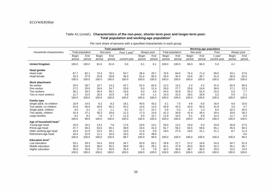
ECO/WKP(99)4

50

Table A1 (contd.). Characteristics of the non-poor, shorter-term poor and longer-term poor:Total population and working-age population1



Beginperiod

Endperiod

Beginperiod


Beginperiod

Endperiod

Beginperiod

Endperiod

Beginperiod

Endperiod

1 year1


Endperiod

United Kingdom 100.0 100.0 61.6 61.6 5.6 6.1 6.1 100.0 100.0 66.3 66.3 5.3 4.1





Young-age head 15.5 10.2 13.3 7.8 17.6 23.5 14.1 20.0 13.2 15.9 9.3 23.9 45.8 27.5Prime-age head 47.7 46.3 53.6 50.1 39.9 23.4 31.0 61.7 59.2 64.5 59.6 55.1 45.5 60.3Older working-age head 20.4 21.5 22.0 26.1 23.0 11.6 5.9 18.4 27.6 19.6 31.1 21.1 8.7 11.4Retirement-age head 16.4 21.9 11.1 16.0 19.2 41.5 48.6 .. .. .. .. .. .. 0.0

100.0 100.0 100.0 100.0 99.7 100.0 99.6 100.0 100.0 100.0 100.0 100.0 100.0 99.2Education level 4


100.0 100.0 100.0 100.0 100.0 100.0 100.0 100.0 100.0 100.0 100.0 100.0 100.0 100.0

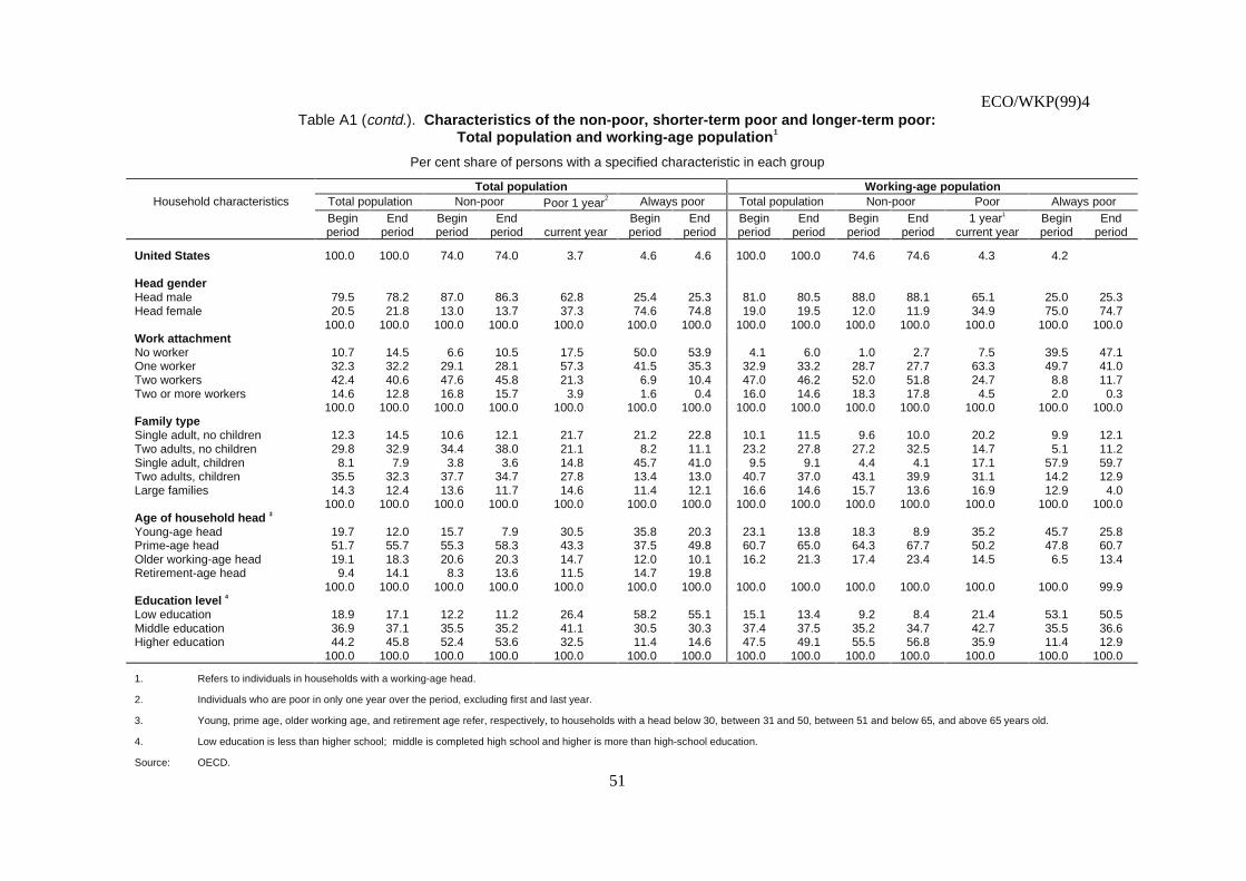
ECO/WKP(99)4

51

Table A1 (contd.). Characteristics of the non-poor, shorter-term poor and longer-term poor:Total population and working-age population1



Beginperiod

Endperiod

Beginperiod


Beginperiod

Endperiod

Beginperiod

Endperiod

Beginperiod

Endperiod

1 year1


Endperiod

United States 100.0 100.0 74.0 74.0 3.7 4.6 4.6 100.0 100.0 74.6 74.6 4.3 4.2





Young-age head 19.7 12.0 15.7 7.9 30.5 35.8 20.3 23.1 13.8 18.3 8.9 35.2 45.7 25.8Prime-age head 51.7 55.7 55.3 58.3 43.3 37.5 49.8 60.7 65.0 64.3 67.7 50.2 47.8 60.7Older working-age head 19.1 18.3 20.6 20.3 14.7 12.0 10.1 16.2 21.3 17.4 23.4 14.5 6.5 13.4Retirement-age head 9.4 14.1 8.3 13.6 11.5 14.7 19.8

100.0 100.0 100.0 100.0 100.0 100.0 100.0 100.0 100.0 100.0 100.0 100.0 100.0 99.9Education level 4


100.0 100.0 100.0 100.0 100.0 100.0 100.0 100.0 100.0 100.0 100.0 100.0 100.0 100.0

1. Refers to individuals in households with a working-age head.

2. Individuals who are poor in only one year over the period, excluding first and last year.

3. Young, prime age, older working age, and retirement age refer, respectively, to households with a head below 30, between 31 and 50, between 51 and below 65, and above 65 years old.

4. Low education is less than higher school; middle is completed high school and higher is more than high-school education.

Source: OECD.

ECO/WKP(99)4

52

2. Analysis of transitions into and out of poverty

2.1. The data set/sample

69. Tables 4 to 8 are based on a data set composed of transitions into and out of poverty. As noted,the time period is defined over the last available six years (1991 to 1996 for Germany and the UnitedKingdom, 1990 to 1995 for Canada, and 1988 to 1993 for the United States). The sample considers allindividuals who remained in the longitudinal data set over the six-year period, but only includes thoseindividuals who where not poor in the first year. All transitions are pooled in a new database. The numberof observations is then equal to the number of individuals times the number of transitions observed foreach individual, thus leading to a larger sample.

2.1.1 Transitions

70. A transition is defined where the individual’s real equivalent household disposable incomebetween two adjacent periods t and t+1 straddles the poverty threshold. Thus, between two adjacentperiods t and t+1 an individual may enter poverty, exit poverty, or may not transit at all (either remainingpoor or non-poor). Certain “events” can occur at the same time as transitions (e.g. a change in theemployment status of a household), while household characteristics can be identified before or after thetransition takes place.

2.1.2 “Events” associated with transitions

71. Following Bane and Ellwood (1986, 1994), Ducan et al. (1993) and, more recently, Maurin andChambaz (1996), various types of “events” are considered to check whether they occur at the time atransition takes place.

- Changes in household employment status includes changes in the number of personsemployed within the household or in hours worked.

- Family structure changes includes, in the case of entries, separation/divorce or achild/relative establishing as a new household. For exits, this category includespartnership/marriage or a child/other becoming spouse. If the relationship of an individual tothe head remains stable43, changes in the size of the family are also considered, distinguishingbetween those due to additional children (e.g. new-born child) and those where there weremore or fewer adults and children (e.g. recomposed families).

- Changes in the components of total household income: Income components considered arehousehold earnings of the household head, spouse and other household workers, capitalincomes (including private transfers), transfer payments received from government and directtaxes and social security contributions paid. Transitions are associated with the incomecomponent contributing the most to the overall change in income.

72. Transitions and “events” are shown in greater detail in Box A1.

43. That is, where there is no household breakdown or formation.

ECO/WKP(99)4

53

2.1.3 Household characteristics

73. Household characteristics are defined as above for the following variables: gender of thehousehold head; employment status of the household44; family type45; age of household head; educationlevel (of the household head). In addition, a variable to control for the cumulative number of years spent inpoverty before entering or exiting poverty was also constructed. Because only a six-year “window” isused, the maximum length of time of the previous time in poverty is three years. The variable is notsymmetric for exits and entry -- i.e. both entering and leaving poverty is associated with the number ofyears in poverty46. These variables are shown in more detail in Box A1.

2.2. Construction of Tables 4 to 7

74. Using the data file for transitions described above, Tables 4 to 7 were constructed in thefollowing manner.

-- Table 4. Distribution of transitions by size of income change

75. Table 4 indicates, in the form of a transition matrix, the frequency of income changes by sizewhich are associated with transitions into or out of poverty. This matrix -- for both entries and exits --shows the originating income range (relatively to the poverty threshold) in the columns and the endingincome range in the rows. This approach differs from simply measuring income variations because thethreshold may also change between the two periods, although the size of these changes is likely to besmall. The number of changes in the range of 10 per cent below the poverty threshold to 10 per cent abovethe poverty threshold is one measure of noise -- i.e. transitions associated with small movements in incomemay be of lesser economic or social consequence.

44. For some purposes, a distinction is made between one worker in one-adult households and in two-adult

households.

45. In some cases, traditional families (e.g. two adults and two children only) were distinguished from largefamilies (e.g. two or more adults with two or more children).

46. It should be noted, however, that true length of the previous spell in poverty cannot be measured accuratelyfor transitions that occur early in the six-year period. Indeed, in the first period no previous periods can bemeasured at all. Thus, for earlier years there will be too few transitions where the individual has hadprevious spells in poverty. The inclusion of year dummies may at least partly control for the biases thatmay result, but it is difficult to judge what the impact will be on the coefficients. In any case, the inclusionof this variable does not affect the other coefficients associated with the other variables. Further tests willbe carried out using a slightly longer period for Germany and the United States.

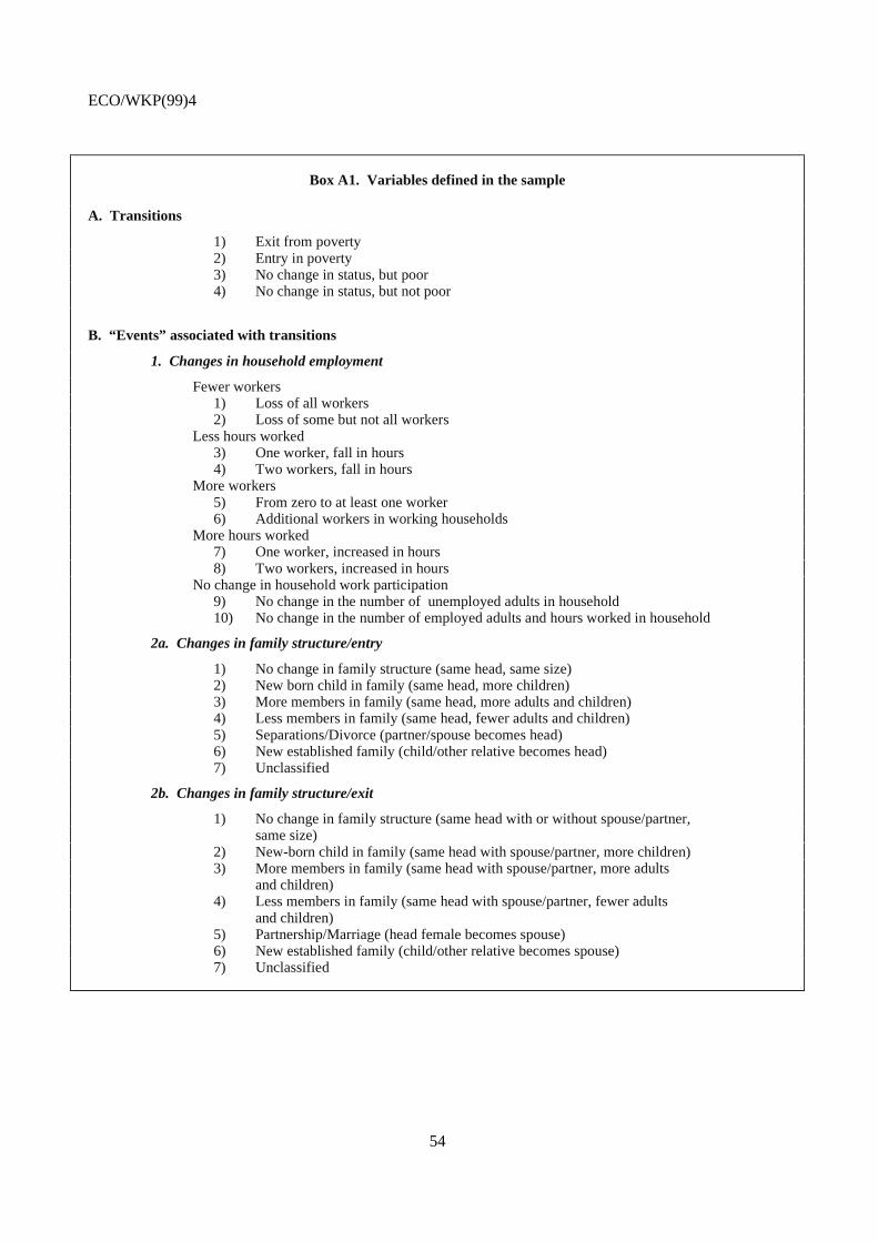
ECO/WKP(99)4

54

Box A1. Variables defined in the sample

A. Transitions

1) Exit from poverty 2) Entry in poverty 3) No change in status, but poor 4) No change in status, but not poor

B. “Events” associated with transitions

1. Changes in household employment

Fewer workers 1) Loss of all workers 2) Loss of some but not all workers Less hours worked 3) One worker, fall in hours 4) Two workers, fall in hours More workers 5) From zero to at least one worker 6) Additional workers in working households More hours worked 7) One worker, increased in hours 8) Two workers, increased in hours No change in household work participation 9) No change in the number of unemployed adults in household 10) No change in the number of employed adults and hours worked in household

2a. Changes in family structure/entry

1) No change in family structure (same head, same size) 2) New born child in family (same head, more children) 3) More members in family (same head, more adults and children) 4) Less members in family (same head, fewer adults and children) 5) Separations/Divorce (partner/spouse becomes head) 6) New established family (child/other relative becomes head) 7) Unclassified

2b. Changes in family structure/exit

1) No change in family structure (same head with or without spouse/partner, same size) 2) New-born child in family (same head with spouse/partner, more children) 3) More members in family (same head with spouse/partner, more adults and children) 4) Less members in family (same head with spouse/partner, fewer adults and children) 5) Partnership/Marriage (head female becomes spouse) 6) New established family (child/other relative becomes spouse) 7) Unclassified

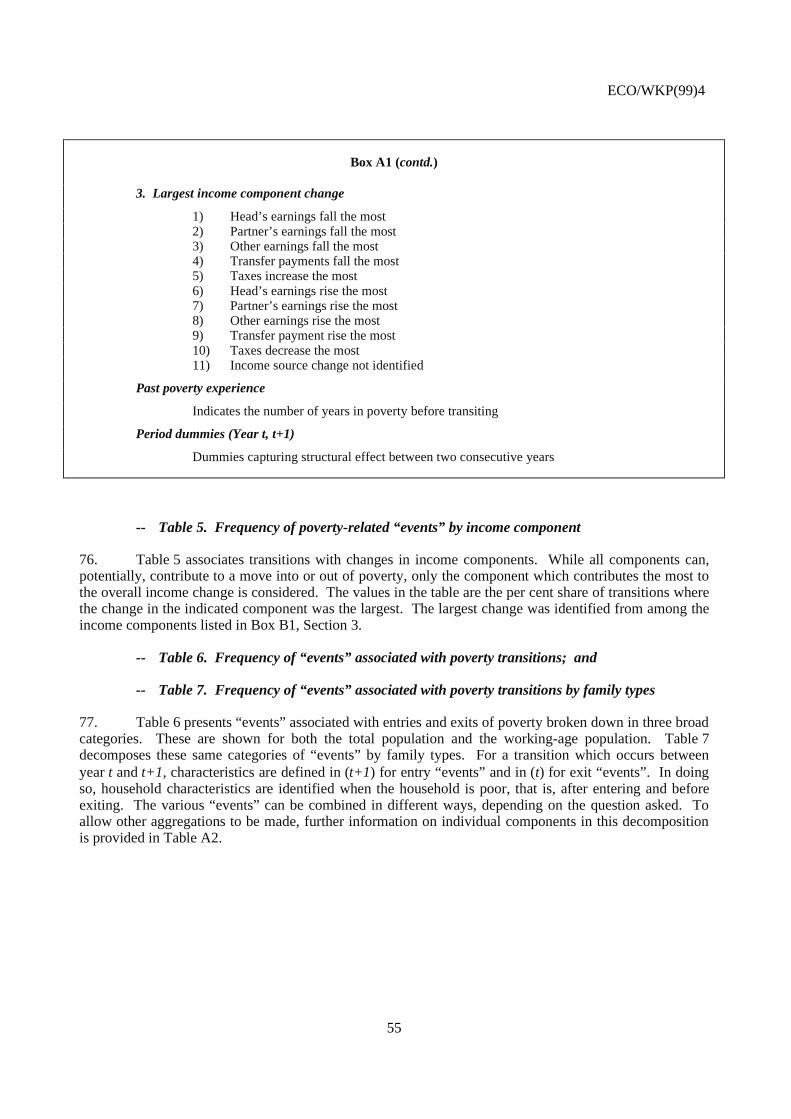
ECO/WKP(99)4

55

Box A1 (contd.)

3. Largest income component change

1) Head’s earnings fall the most 2) Partner’s earnings fall the most 3) Other earnings fall the most 4) Transfer payments fall the most 5) Taxes increase the most 6) Head’s earnings rise the most 7) Partner’s earnings rise the most 8) Other earnings rise the most 9) Transfer payment rise the most 10) Taxes decrease the most 11) Income source change not identified

Past poverty experience

Indicates the number of years in poverty before transiting

Period dummies (Year t, t+1)

Dummies capturing structural effect between two consecutive years

-- Table 5. Frequency of poverty-related “events” by income component

76. Table 5 associates transitions with changes in income components. While all components can,potentially, contribute to a move into or out of poverty, only the component which contributes the most tothe overall income change is considered. The values in the table are the per cent share of transitions wherethe change in the indicated component was the largest. The largest change was identified from among theincome components listed in Box B1, Section 3.

-- Table 6. Frequency of “events” associated with poverty transitions; and

-- Table 7. Frequency of “events” associated with poverty transitions by family types

77. Table 6 presents “events” associated with entries and exits of poverty broken down in three broadcategories. These are shown for both the total population and the working-age population. Table 7decomposes these same categories of “events” by family types. For a transition which occurs betweenyear t and t+1, characteristics are defined in (t+1) for entry “events” and in (t) for exit “events”. In doingso, household characteristics are identified when the household is poor, that is, after entering and beforeexiting. The various “events” can be combined in different ways, depending on the question asked. Toallow other aggregations to be made, further information on individual components in this decompositionis provided in Table A2.

ECO/WKP(99)4

56

2.2.1 Main categories of “events” used in Tables 6 and 7

78. For the purposes of this study, the various “events” were regrouped into three categories. Theexamples below are given for transitions into poverty. Cases for transition out of poverty are symmetric,but note that the categories for exits change somewhat (see Table 6 and Box A1)47.

2.2.1.1 Employment/earnings-related “events”

79. These refer to changes in employment status, hours and wage rates within a stable familystructure. For entry, employment/earnings “events” include:

- Cases where there are: “fewer workers”, “less hours worked” and “no change in familystructure”.

- Cases where there are: “fewer workers”, “less hours worked” where this occurs at the sametime as an increase in family needs (including “more members” and “new-born child” infamily). The remainder of employment cases are included in “other events”.

- Cases where there are: “no change in the number of employed adults and hours worked inhousehold” and “no change in family structure” and where the head’s, partner’s or otherfamily workers’ earnings fall the most. (Changes in other income sources are included in thecategory of “other events”.)

2.2.1.2 Family structure-related “events”

80. These are mainly cases related to separations/divorce (partnership/marriage in the case of exits)and children or other family members forming new households. In all of these cases, changes in householdwork participation generally follow from this change in household status. For example, a separation of atwo-earner household leads to two one-earner households. Such changes in employment status do notoccur because of a change in the employment status of the two individuals. For this reason, this group istreated separately from other employment status changes indicated in the preceding group. For entry, thiscategory includes:

- Cases of: “separations/divorce” and “fewer workers”, “less hours worked” or “no change inhousehold work participation”. (Cases where there are “more workers” or “more hoursworked” are included in the category of “other events”.)

- Cases where there are: “newly-established families” and “fewer workers” or “less hoursworked” or “no change in household work participation”. (Cases where there are “moreworkers” or “more hours worked” will be included in the category of “other events”.)

- Cases where there are: “less members in family” (e.g. the head is left (alone) with feweradults and children) and where there are “fewer workers”. (The remainder of employmentcases will be included in the category of “other events”.)

47. For example, in the case of employment/earnings-related “events” associated to exit, “fewer workers”

becomes “more workers”.

ECO/WKP(99)4

57

2.2.1.3. Other “events”

81. These include a range of special categories which do not fit easily into the first two categories,but essentially cover transitions where there is no change either in employment/earnings and family status“events”. For example, a person remains unemployed in the two periods but enters poverty. Sinceemployment or earnings-related “events” have already been included in “employment/earnings-related“events”, this must reflect changes in other market income, transfers and taxes. Further analysis of the datasuggests that the bulk of these movements appear to occur where transfer payments and capital incomesare the largest change. “Other ‘events’” includes:

- Cases where there are: “no change in the number of unemployed adults” in both periods and“no change in family structure”.

- Cases where there are: “no change in the number of employed adults and hours worked”,“no change in family structure” and where other income sources except earnings fall the most(the latter are included in “employment/earnings-related ‘events’”).

- Of those unemployed and employed in both periods, the table distinguishes betweenhouseholds who enter poverty when the fall in transfer payments or the fall in capital incomemakes up the largest component of the fall in income. Approximately 90 per cent of thesetransitions are associated with the fall in these two components.

- A residual labelled “Else” which includes cases where there are: a) “more workers”, “morehours worked” and “changes in family structure”; and b) the remainder of“family-structure-related events” associated to entries. Symmetric cases have to consideredfor exits.

2.3. Estimates of the probability of exit and entry (Table 8)

2.3.1 Methodological issues

82. While Tables 6 and 7 show the frequency of “events” associated to entries or exits, they do notshow whether an individual experiencing an “event” is more likely to enter or exit poverty. Estimates ofthe probability of exit or entry when an “event” occurs, capture such information: these show whether ornot an “event” increases the chances of exit or entry. These estimates permit a comparison of which“events” most affect the probability of moving into or out of poverty48. The estimation procedure in thissection is based on logit models shown in Box A2 (see Maddala, [1997] and Pindyck and Rubinfeld[1981]).

83. As noted in the main text, these results should be interpreted more as descriptions of exitingpatterns rather than causal relations. While it is tempting to see, say, a change in employment status as thecause of poverty entry, the change in employment status itself is the result of a range of market andinstitutional factors which make up the true factors affecting household behaviour. These have not beenaddressed here.

48. The key feature of logit estimates is that, considering all “events” at the same time, it is then possible not

only to separate simultaneous “events”, but to test interacting effects and to identify those having thestrongest impact on the probability to transit when all others are held constant. These logit models do notintend to provide a full explanation of transitions.

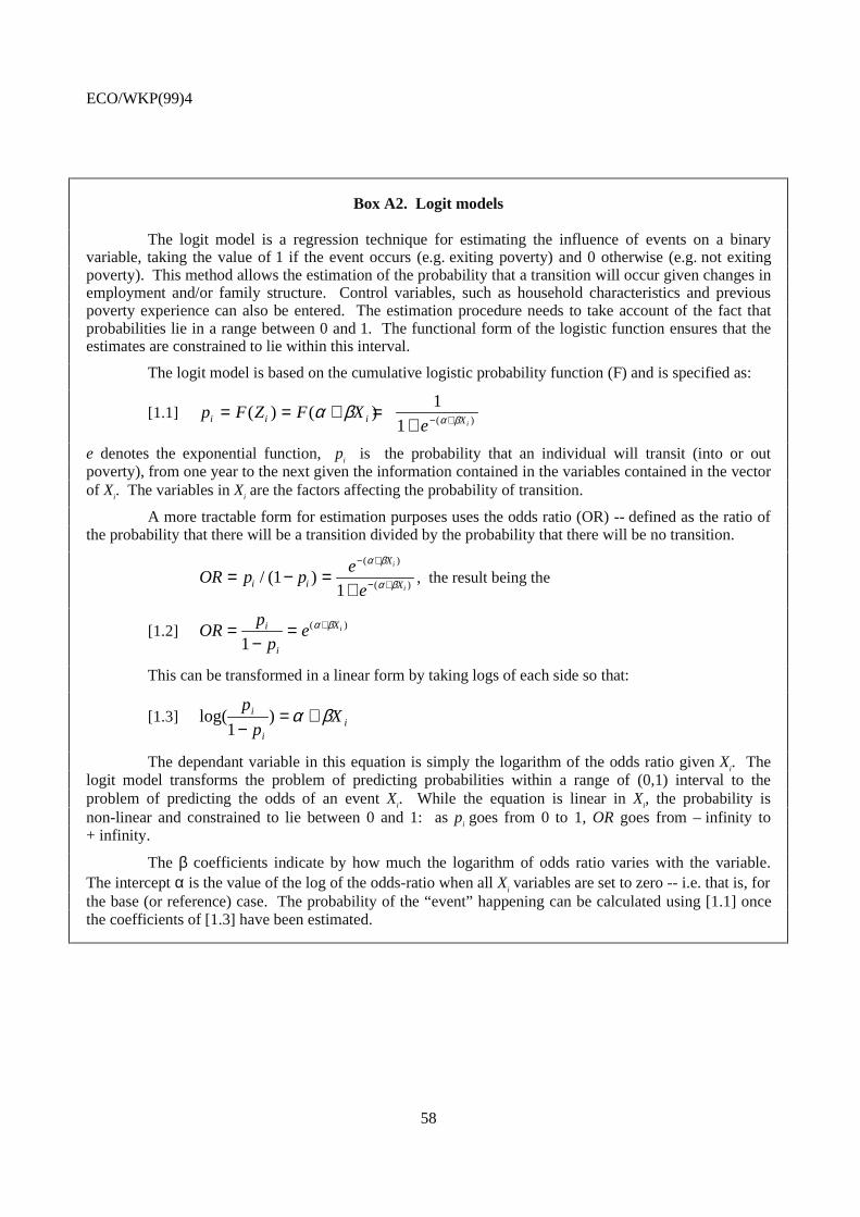
ECO/WKP(99)4

58

Box A2. Logit models

The logit model is a regression technique for estimating the influence of events on a binaryvariable, taking the value of 1 if the event occurs (e.g. exiting poverty) and 0 otherwise (e.g. not exitingpoverty). This method allows the estimation of the probability that a transition will occur given changes inemployment and/or family structure. Control variables, such as household characteristics and previouspoverty experience can also be entered. The estimation procedure needs to take account of the fact thatprobabilities lie in a range between 0 and 1. The functional form of the logistic function ensures that theestimates are constrained to lie within this interval.

The logit model is based on the cumulative logistic probability function (F) and is specified as:

[1.1] p F Z F Xei i i Xi

= = + =+ − +( ) ( )

( )α β α β

1

1

e denotes the exponential function, pi is the probability that an individual will transit (into or outpoverty), from one year to the next given the information contained in the variables contained in the vectorof Xi. The variables in Xi are the factors affecting the probability of transition.

A more tractable form for estimation purposes uses the odds ratio (OR) -- defined as the ratio ofthe probability that there will be a transition divided by the probability that there will be no transition.

OR p pe

ei i

X

X

i

i= − =

+

− +

− +/ ( )( )

( )11

α β

α β , the result being the

[1.2] ORp

pei

i

Xi=−

= +

1( )α β

This can be transformed in a linear form by taking logs of each side so that:

[1.3] ii

i Xp

p βα +=−

)1

log(

The dependant variable in this equation is simply the logarithm of the odds ratio given Xi. Thelogit model transforms the problem of predicting probabilities within a range of (0,1) interval to theproblem of predicting the odds of an event Xi. While the equation is linear in Xi, the probability isnon-linear and constrained to lie between 0 and 1: as pi goes from 0 to 1, OR goes from – infinity to+ infinity.

The β coefficients indicate by how much the logarithm of odds ratio varies with the variable.The intercept α is the value of the log of the odds-ratio when all Xi variables are set to zero -- i.e. that is, forthe base (or reference) case. The probability of the “event” happening can be calculated using [1.1] oncethe coefficients of [1.3] have been estimated.

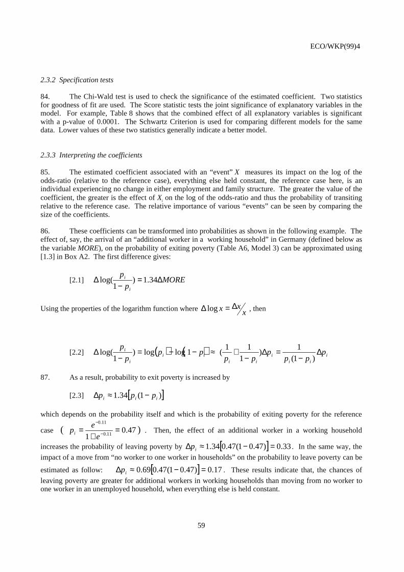
ECO/WKP(99)4

59

2.3.2 Specification tests

84. The Chi-Wald test is used to check the significance of the estimated coefficient. Two statisticsfor goodness of fit are used. The Score statistic tests the joint significance of explanatory variables in themodel. For example, Table 8 shows that the combined effect of all explanatory variables is significantwith a p-value of 0.0001. The Schwartz Criterion is used for comparing different models for the samedata. Lower values of these two statistics generally indicate a better model.

2.3.3 Interpreting the coefficients

85. The estimated coefficient associated with an “event” X measures its impact on the log of theodds-ratio (relative to the reference case), everything else held constant, the reference case here, is anindividual experiencing no change in either employment and family structure. The greater the value of thecoefficient, the greater is the effect of Xi on the log of the odds-ratio and thus the probability of transitingrelative to the reference case. The relative importance of various “events” can be seen by comparing thesize of the coefficients.

86. These coefficients can be transformed into probabilities as shown in the following example. Theeffect of, say, the arrival of an “additional worker in a working household” in Germany (defined below asthe variable MORE), on the probability of exiting poverty (Table A6, Model 3) can be approximated using[1.3] in Box A2. The first difference gives:

[2.1] MOREp

p

i

i ∆=−

∆ 34.1)1

log(

Using the properties of the logarithm function where ∆ ∆log x xx= , then

[2.2] ( ) ( ) iii

iii

iii

i ppp

ppp

ppp

p∆

−=∆

−+≈−−=

−∆

)1(

1)

1

11(1loglog)

1log(

87. As a result, probability to exit poverty is increased by

[2.3] [ ])1(34.1 iii ppp −≈∆

which depends on the probability itself and which is the probability of exiting poverty for the reference

case ( 47.01 11.0

11.0

=+

= −

−

e

epi ) . Then, the effect of an additional worker in a working household

increases the probability of leaving poverty by [ ] 33.0)47.01(47.034.1 =−≈∆ ip . In the same way, the

impact of a move from “no worker to one worker in households” on the probability to leave poverty can be

estimated as follow: [ ] 17.0)47.01(47.069.0 =−≈∆ ip . These results indicate that, the chances of

leaving poverty are greater for additional workers in working households than moving from no worker toone worker in an unemployed household, when everything else is held constant.

ECO/WKP(99)4

60

2.3.4 Results

88. Table 8 shows the factors that affect: 1) the probability of entering poverty for all non-poorindividuals; and 2) the probability of exiting poverty for all poor individuals. All variables are dummies,with one category omitted to avoid collinearity. The remaining categories were captured by the intercept(the reference case).

89. A first set of models estimates the combined impact of employment and family "events" on theprobability of transiting into or out of poverty -- i.e. equations with right-hand crossed variables (models 1and 2). Then, a second set of models (models 3 and 4) is run to measure the effect of family (employment)related "events", independent of changes in employment (family) related "events" –i.e. equations withuncrossed variables. Control variables for household characteristics prior to transition (i.e. educationlevels, age of household heads), past poverty experience and period dummies were also introduced toassess coefficient stability. Both types of models produce similar results:

í employment events have a larger impact on the probability of transiting into poverty than familyevents;

í combined (crossed) family and employment variables have, in all countries, stronger effects thanthose when only one type of change occurs at the same time (uncrossed variables);

90. In a second step, additional control variables were added to allow for family and work type in theperiod preceding transitions, thus accounting for the fact that transition probabilities tend to be stronger forcertain "at risk" subgroups. These additional variables generally improve the fit without changing the keyresults of the two models. The results confirm that:

í single parents show higher and significant coefficients compared to other family types for entryprobabilities, except in Canada. More workers in the households, lowers the risk of falling intopoverty, irrespective of changes in employment and/or family status;

í by contrast, the coefficients are negative and significant for single parents for exit probabilities(except in Canada) while those for households with more than two workers are positive, large andsignificant (except in Germany where these households appear to have enough incomes to remainalways above the poverty line);

ECO/WKP(99)4

61

Table A2. Frequency of poverty-related “events”: further decomposition of the main categories of “events” Germany

ENTRIESTotal

populationWorking-agepopulation EXITS

Totalpopulation

Working-agepopulation

Employment/earnings-related events 47.5 51.5 Employment/earnings-related events 47.5 52.4

Change in employment only (same family structure,same size) 25.1 27.3


Loss of all workers 8.2 8.6 From zero to at least one worker 9.6 10.4Loss of some but not all workers 6.5 7.1 Additional workers in working households 5.3 5.9One worker fall in hours 7.9 8.8 One worker increase in hours 12.1 13.3More than one worker fall in hours 2.5 2.8 More than one worker increase in hours 0.8 0.9

Change in employment and increased family needs 8.3 9.0 Change in employment and increased family needs 1.3 1.5Same number of workers 3.5 3.8 Same number of workers 0.9 1.0Loss of workers, including all workers 4.1 4.4 From zero to at least one worker 0.0 0.0More workers 0.7 0.8 Additional workers in working households 0.4 0.5

No change in employment status and family structure No change in employment status and family structureTotal earnings fall the most 14.1 15.2 Total earnings rise the most 18.4 20.4

Family-structure-related 23.9 24.3 Family-structure-related 13.1 14.5

Separations/divorce (spouse becomes head) 7.2 7.1 Partnership/marriage (head becomes spouse) 0.3 0.3

New established households (child,relative becomes head)

9.7 9.6 New established households (child,relative becomes spouse)

9.4 10.4

Fewer members (head is left with fewer adultsor children) 7.0 7.6

More members (head with additional adultsor children) 3.4 3.8

Other factors (no change in employment and familystatus)

23.1 18.2 Other factors (no change in employment and familystatus)

32.1 25.4

Unemployed households 16.0 10.5 Unemployed households 20.1 13.1Employed households 7.1 7.7 Employed households 12.0 12.3

Of which transfers and capital incomes fallthe most for both unemployed and employedhouseholds

(21.9) (17.0)of which transfers and capital incomes risethe most for both unemployed and employedhouseholds

(26.5) (20.8)

Else 5.5 6.0 Else 7.3 7.7

Total 100.0 100.0 Total 100.0 100.0

ECO/WKP(99)4

62

Table A2 (contd.). Frequency of poverty-related “events”: further decomposition of the main categories of “events” United Kingdom

ENTRIESTotal


Totalpopulation










New established households (child,relative becomes head) 7.8 9.8

New established households (child,relative becomes spouse) 1.1 1.4





41.4 27.1




(39.0) (24.5)

Else 10.8 13.5 Else 8.7 11.1

Total 100.0 100.0 Total 100.0 100.0

ECO/WKP(99)4

63

Table A2 (contd.). Frequency of poverty-related “events”: further decomposition of the main categories of “events” United States

ENTRIESTotal


Totalpopulation










New established households (child,relative becomes head) 6.0 6.5

New established households (child,relative becomes spouse) 1.5 1.6





11.4 7.7




(10.8) (7.4)

Else 8.3 8.9 Else 12.2 12.2

Total 100.0 100.0 Total 100.0 100.0

Source: OECD.

ECO/WKP(99)4

64

Table A3. Entry model: crossed variables

Model 1 Model 2

VariablesCanadaEstimate

GermanyEstimate

United KingdomEstimate

United StatesEstimate

CanadaEstimate

GermanyEstimate



Intercept -2.21** -2.82** -2.29** -2.79** -1.89** -1.30** -0.42** -1.40**

No change in employment andfamily structure

Base Base base base base Base base base

No change in employment statusand family status

Employment status change/no change in family status

Loss of all workers 2.34** 2.81** 1.65** 2.32** 2.48** 3.05** 2.12** 2.47**Loss of some but not all workers 0.71** 0.76** 0.03 1.35** 1.45** 1.92** 1.22** 2.19**One worker fall in hours 2.03** 1.03** 1.69** 1.99** 1.09** 1.33**More than one worker fall inhours

0.15 -1.48** 0.18 1.22** -0.54 0.89**

Other change -0.31** -0.78** 0.05 -0.45** -0.42** -0.68** 0.08 -0.46**

Change in family status/nochange in employment status

Separations/divorce (spousebecomes head)

2.74** 0.72** 1.14** 0.73** 2.59** 0.84** 1.01**

Child becomes head 2.38** 0.47* 1.59** 2.72** 0.79** 2.02**Other adult becomes head 0.89* 0.67* -0.25 1.91* 0.58 0.10Arrival of children 0.01 0.89** 0.39** 0.13 0.68** 0.53**More members 1.38** -0.42 1.16** 0.83** 0.70** -0.71 1.21**Less members 0.04 0.37* -0.13 0.26* 0.32 0.64** 0.11

Simultaneous changes inemployment and family status

Loss of all workers


5.36** 3.75** 3.95** 3.20** 5.57** 4.06** 4.10**

Child becomes head 5.62** 5.05** 6.71** 6.21**Other adult becomes head 4.57** 2.68** 5.22** 3.13**Arrival of children 3.71** 2.23** 3.13** 4.25** 2.49** 3.45**More members 4.02**Less members 3.36** 2.46** 3.13** 2.79** 4.16** 3.24** 3.60**

Loss of some but not all workers


2.08** 2.91** 1.12** 3.34** 2.82** 3.94** 2.36** 4.08**

Child becomes head 2.57** 1.03** 2.79** 4.10** 2.63** 4.00**Other adult becomes head 3.22** -0.28 1.28** 4.64** 1.44* 2.51**Arrival of children 1.04** 1.45** -0.43 1.60** 1.67** 2.46** 0.74 2.31**More members 0.88** 2.03** 1.87** 1.81** 3.68** 2.73**Less members 0.76** 0.80** 0.43** 0.83** 1.74** 2.15** 1.91** 1.89**

One worker fall in hours


1.80 2.85** 4.40** 2.06 3.10** 3.89**

Child becomes head 3.12* 4.27** 5.84** 3.14* 3.81**Other adult becomes head 5.62** 1.51 1.34Arrival of children 3.21** 3.42** 3.05** 2.99**More members 3.92** 1.87** 3.66** 1.46**Less members 2.65** 2.33** 2.05** 2.77** 1.52**

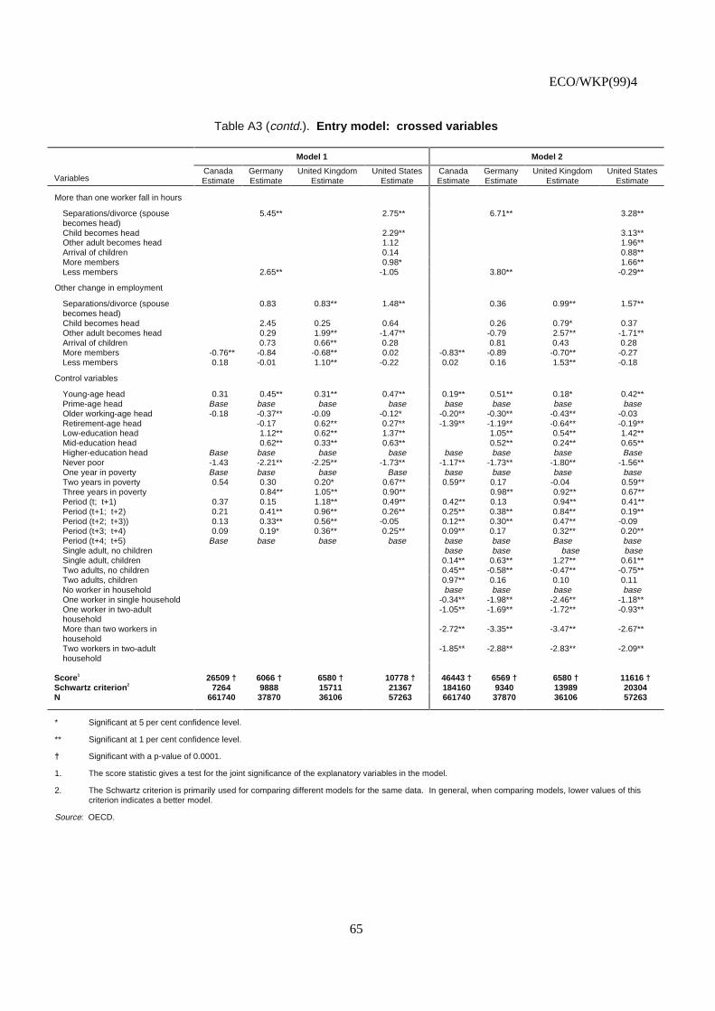
ECO/WKP(99)4

65

Table A3 (contd.). Entry model: crossed variables

Model 1 Model 2


GermanyEstimate



CanadaEstimate

GermanyEstimate



More than one worker fall in hours


5.45** 2.75** 6.71** 3.28**

Child becomes head 2.29** 3.13**Other adult becomes head 1.12 1.96**Arrival of children 0.14 0.88**More members 0.98* 1.66**Less members 2.65** -1.05 3.80** -0.29**

Other change in employment


0.83 0.83** 1.48** 0.36 0.99** 1.57**

Child becomes head 2.45 0.25 0.64 0.26 0.79* 0.37Other adult becomes head 0.29 1.99** -1.47** -0.79 2.57** -1.71**Arrival of children 0.73 0.66** 0.28 0.81 0.43 0.28More members -0.76** -0.84 -0.68** 0.02 -0.83** -0.89 -0.70** -0.27Less members 0.18 -0.01 1.10** -0.22 0.02 0.16 1.53** -0.18

Control variables

Young-age head 0.31 0.45** 0.31** 0.47** 0.19** 0.51** 0.18* 0.42**Prime-age head Base base base base base base base baseOlder working-age head -0.18 -0.37** -0.09 -0.12* -0.20** -0.30** -0.43** -0.03Retirement-age head -0.17 0.62** 0.27** -1.39** -1.19** -0.64** -0.19**Low-education head 1.12** 0.62** 1.37** 1.05** 0.54** 1.42**Mid-education head 0.62** 0.33** 0.63** 0.52** 0.24** 0.65**Higher-education head Base base base base base base base BaseNever poor -1.43 -2.21** -2.25** -1.73** -1.17** -1.73** -1.80** -1.56**One year in poverty Base base base Base base base base baseTwo years in poverty 0.54 0.30 0.20* 0.67** 0.59** 0.17 -0.04 0.59**Three years in poverty 0.84** 1.05** 0.90** 0.98** 0.92** 0.67**Period (t; t+1) 0.37 0.15 1.18** 0.49** 0.42** 0.13 0.94** 0.41**Period (t+1; t+2) 0.21 0.41** 0.96** 0.26** 0.25** 0.38** 0.84** 0.19**Period (t+2; t+3)) 0.13 0.33** 0.56** -0.05 0.12** 0.30** 0.47** -0.09Period (t+3; t+4) 0.09 0.19* 0.36** 0.25** 0.09** 0.17 0.32** 0.20**Period (t+4; t+5) Base base base base base base Base baseSingle adult, no children base base base baseSingle adult, children 0.14** 0.63** 1.27** 0.61**Two adults, no children 0.45** -0.58** -0.47** -0.75**Two adults, children 0.97** 0.16 0.10 0.11No worker in household base base base baseOne worker in single household -0.34** -1.98** -2.46** -1.18**One worker in two-adulthousehold

-1.05** -1.69** -1.72** -0.93**

More than two workers inhousehold

-2.72** -3.35** -3.47** -2.67**

Two workers in two-adulthousehold

-1.85** -2.88** -2.83** -2.09**

Score1 26509 † 6066 † 6580 † 10778 † 46443 † 6569 † 6580 † 11616 †Schwartz criterion 2 7264 9888 15711 21367 184160 9340 13989 20304N 661740 37870 36106 57263 661740 37870 36106 57263





2. The Schwartz criterion is primarily used for comparing different models for the same data. In general, when comparing models, lower values of thiscriterion indicates a better model.

Source: OECD.

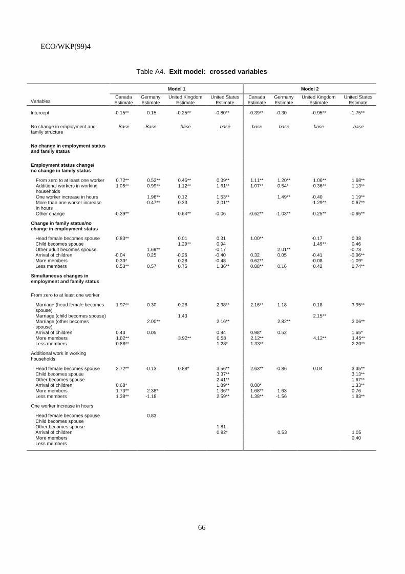
ECO/WKP(99)4

66

Table A4. Exit model: crossed variables

Model 1 Model 2


GermanyEstimate



CanadaEstimate

GermanyEstimate



Intercept -0.15** 0.15 -0.25** -0.80** -0.39** -0.30 -0.95** -1.75**

No change in employment andfamily structure

Base Base base base base base base base

No change in employment statusand family status

Employment status change/no change in family status

From zero to at least one worker 0.72** 0.53** 0.45** 0.39** 1.11** 1.20** 1.06** 1.68**Additional workers in workinghouseholds

1.05** 0.99** 1.12** 1.61** 1.07** 0.54* 0.36** 1.13**

One worker increase in hours 1.96** 0.12 1.53** 1.49** -0.40 1.19**More than one worker increasein hours

-0.47** 0.33 2.01** -1.29** 0.67**

Other change -0.39** 0.64** -0.06 -0.62** -1.03** -0.25** -0.95**

Change in family status/nochange in employment status

Head female becomes spouse 0.83** 0.01 0.31 1.00** -0.17 0.38Child becomes spouse 1.29** 0.94 1.49** 0.46Other adult becomes spouse 1.69** -0.17 2.01** -0.78Arrival of children -0.04 0.25 -0.26 -0.40 0.32 0.05 -0.41 -0.96**More members 0.33* 0.28 -0.48 0.62** -0.08 -1.09*Less members 0.53** 0.57 0.75 1.36** 0.88** 0.16 0.42 0.74**

Simultaneous changes inemployment and family status

From zero to at least one worker

Marriage (head female becomesspouse)

1.97** 0.30 -0.28 2.38** 2.16** 1.18 0.18 3.95**

Marriage (child becomes spouse) 1.43 2.15**Marriage (other becomesspouse)

2.00** 2.16** 2.82** 3.06**

Arrival of children 0.43 0.05 0.84 0.98* 0.52 1.65*More members 1.82** 3.92** 0.58 2.12** 4.12** 1.45**Less members 0.88** 1.28* 1.33** 2.20**

Additional work in workinghouseholds

Head female becomes spouse 2.72** -0.13 0.88* 3.56** 2.63** -0.86 0.04 3.35**Child becomes spouse 3.37** 3.13**Other becomes spouse 2.41** 1.67**Arrival of children 0.68* 1.89** 0.80* 1.33**More members 1.73** 2.38* 1.36** 1.68** 1.63 0.76Less members 1.38** -1.18 2.59** 1.38** -1.56 1.83**

One worker increase in hours

Head female becomes spouse 0.83Child becomes spouseOther becomes spouse 1.81Arrival of children 0.92* 0.53 1.05More members 0.40Less members

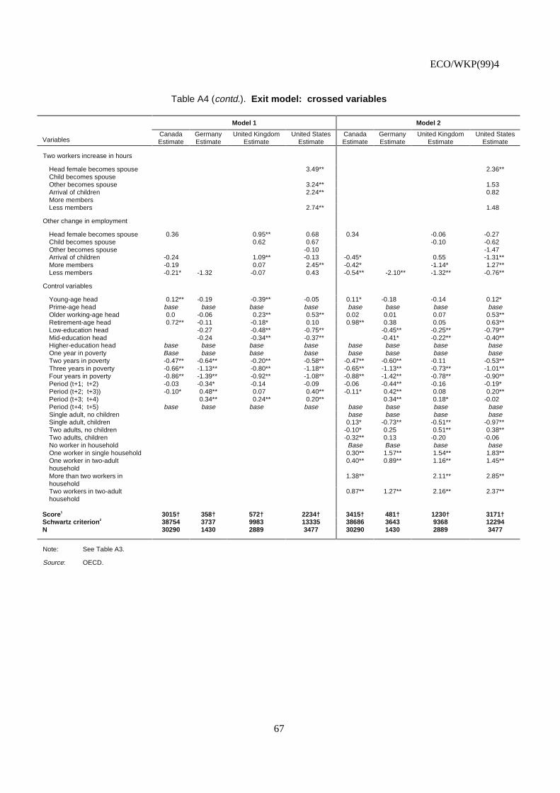
ECO/WKP(99)4

67

Table A4 (contd.). Exit model: crossed variables

Model 1 Model 2


GermanyEstimate



CanadaEstimate

GermanyEstimate



Two workers increase in hours

Head female becomes spouse 3.49** 2.36**Child becomes spouseOther becomes spouse 3.24** 1.53Arrival of children 2.24** 0.82More membersLess members 2.74** 1.48

Other change in employment

Head female becomes spouse 0.36 0.95** 0.68 0.34 -0.06 -0.27Child becomes spouse 0.62 0.67 -0.10 -0.62Other becomes spouse -0.10 -1.47Arrival of children -0.24 1.09** -0.13 -0.45* 0.55 -1.31**More members -0.19 0.07 2.45** -0.42* -1.14* 1.27**Less members -0.21* -1.32 -0.07 0.43 -0.54** -2.10** -1.32** -0.76**

Control variables

Young-age head 0.12** -0.19 -0.39** -0.05 0.11* -0.18 -0.14 0.12*Prime-age head base base base base base base base baseOlder working-age head 0.0 -0.06 0.23** 0.53** 0.02 0.01 0.07 0.53**Retirement-age head 0.72** -0.11 -0.18* 0.10 0.98** 0.38 0.05 0.63**Low-education head -0.27 -0.48** -0.75** -0.45** -0.25** -0.79**Mid-education head -0.24 -0.34** -0.37** -0.41* -0.22** -0.40**Higher-education head base base base base base base base baseOne year in poverty Base base base base base base base baseTwo years in poverty -0.47** -0.64** -0.20** -0.58** -0.47** -0.60** -0.11 -0.53**Three years in poverty -0.66** -1.13** -0.80** -1.18** -0.65** -1.13** -0.73** -1.01**Four years in poverty -0.86** -1.39** -0.92** -1.08** -0.88** -1.42** -0.78** -0.90**Period (t+1; t+2) -0.03 -0.34* -0.14 -0.09 -0.06 -0.44** -0.16 -0.19*Period (t+2; t+3)) -0.10* 0.48** 0.07 0.40** -0.11* 0.42** 0.08 0.20**Period (t+3; t+4) 0.34** 0.24** 0.20** 0.34** 0.18* -0.02Period (t+4; t+5) base base base base base base base baseSingle adult, no children base base base baseSingle adult, children 0.13* -0.73** -0.51** -0.97**Two adults, no children -0.10* 0.25 0.51** 0.38**Two adults, children -0.32** 0.13 -0.20 -0.06No worker in household Base Base base baseOne worker in single household 0.30** 1.57** 1.54** 1.83**One worker in two-adulthousehold

0.40** 0.89** 1.16** 1.45**


1.38** 2.11** 2.85**


0.87** 1.27** 2.16** 2.37**

Score1 3015† 358† 572† 2234† 3415† 481† 1230† 3171†Schwartz criterion 2 38754 3737 9983 13335 38686 3643 9368 12294N 30290 1430 2889 3477 30290 1430 2889 3477

Note: See Table A3.

Source: OECD.

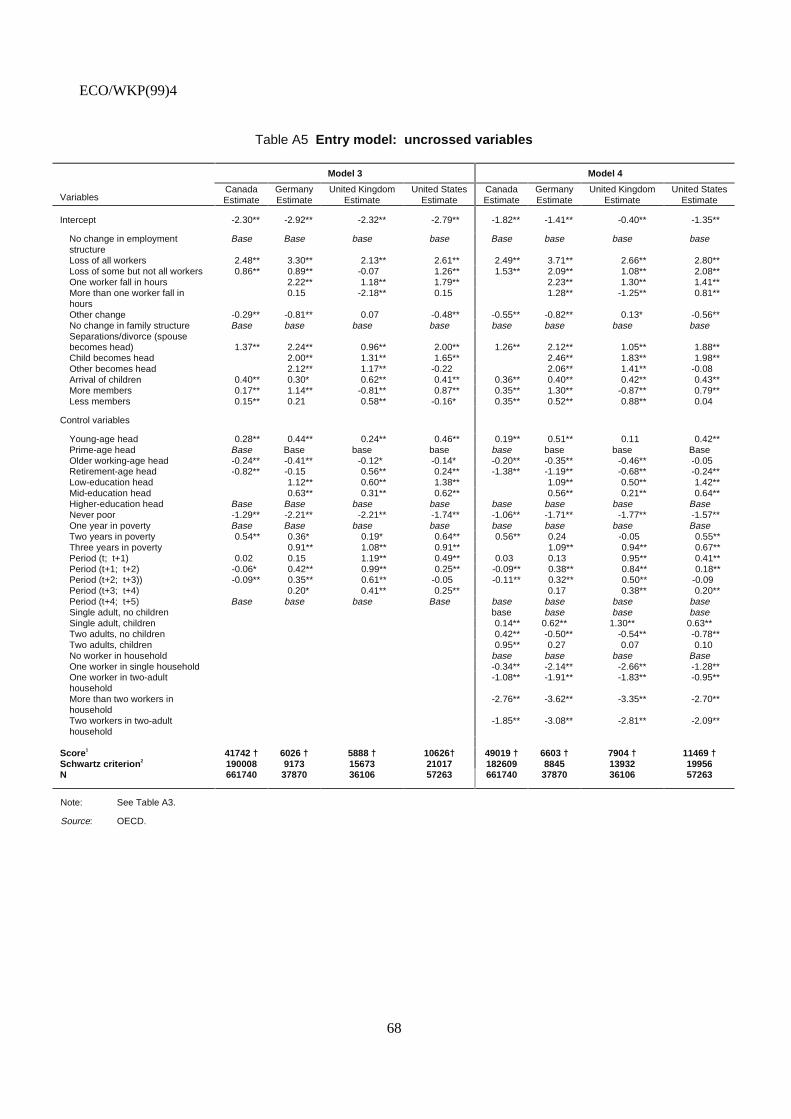
ECO/WKP(99)4

68

Table A5 Entry model: uncrossed variables

Model 3 Model 4


GermanyEstimate



CanadaEstimate

GermanyEstimate



Intercept -2.30** -2.92** -2.32** -2.79** -1.82** -1.41** -0.40** -1.35**

No change in employmentstructure

Base Base base base Base base base base

Loss of all workers 2.48** 3.30** 2.13** 2.61** 2.49** 3.71** 2.66** 2.80**Loss of some but not all workers 0.86** 0.89** -0.07 1.26** 1.53** 2.09** 1.08** 2.08**One worker fall in hours 2.22** 1.18** 1.79** 2.23** 1.30** 1.41**More than one worker fall inhours

0.15 -2.18** 0.15 1.28** -1.25** 0.81**

Other change -0.29** -0.81** 0.07 -0.48** -0.55** -0.82** 0.13* -0.56**No change in family structure Base base base base base base base baseSeparations/divorce (spousebecomes head) 1.37** 2.24** 0.96** 2.00** 1.26** 2.12** 1.05** 1.88**Child becomes head 2.00** 1.31** 1.65** 2.46** 1.83** 1.98**Other becomes head 2.12** 1.17** -0.22 2.06** 1.41** -0.08Arrival of children 0.40** 0.30* 0.62** 0.41** 0.36** 0.40** 0.42** 0.43**More members 0.17** 1.14** -0.81** 0.87** 0.35** 1.30** -0.87** 0.79**Less members 0.15** 0.21 0.58** -0.16* 0.35** 0.52** 0.88** 0.04

Control variables

Young-age head 0.28** 0.44** 0.24** 0.46** 0.19** 0.51** 0.11 0.42**Prime-age head Base Base base base base base base BaseOlder working-age head -0.24** -0.41** -0.12* -0.14* -0.20** -0.35** -0.46** -0.05Retirement-age head -0.82** -0.15 0.56** 0.24** -1.38** -1.19** -0.68** -0.24**Low-education head 1.12** 0.60** 1.38** 1.09** 0.50** 1.42**Mid-education head 0.63** 0.31** 0.62** 0.56** 0.21** 0.64**Higher-education head Base Base base base base base base BaseNever poor -1.29** -2.21** -2.21** -1.74** -1.06** -1.71** -1.77** -1.57**One year in poverty Base Base base base base base base BaseTwo years in poverty 0.54** 0.36* 0.19* 0.64** 0.56** 0.24 -0.05 0.55**Three years in poverty 0.91** 1.08** 0.91** 1.09** 0.94** 0.67**Period (t; t+1) 0.02 0.15 1.19** 0.49** 0.03 0.13 0.95** 0.41**Period (t+1; t+2) -0.06* 0.42** 0.99** 0.25** -0.09** 0.38** 0.84** 0.18**Period (t+2; t+3)) -0.09** 0.35** 0.61** -0.05 -0.11** 0.32** 0.50** -0.09Period (t+3; t+4) 0.20* 0.41** 0.25** 0.17 0.38** 0.20**Period (t+4; t+5) Base base base Base base base base baseSingle adult, no children base base base baseSingle adult, children 0.14** 0.62** 1.30** 0.63**Two adults, no children 0.42** -0.50** -0.54** -0.78**Two adults, children 0.95** 0.27 0.07 0.10No worker in household base base base BaseOne worker in single household -0.34** -2.14** -2.66** -1.28**One worker in two-adulthousehold

-1.08** -1.91** -1.83** -0.95**


-2.76** -3.62** -3.35** -2.70**


-1.85** -3.08** -2.81** -2.09**

Score1 41742 † 6026 † 5888 † 10626† 49019 † 6603 † 7904 † 11469 †Schwartz criterion 2 190008 9173 15673 21017 182609 8845 13932 19956N 661740 37870 36106 57263 661740 37870 36106 57263

Note: See Table A3.

Source: OECD.

ECO/WKP(99)4

69

Table A6. Exit model: uncrossed variables

Model 3 Model 4


GermanyEstimate



CanadaEstimate

GermanyEstimate



Intercept -0.21** -0.11 -0.40** -0.82** -0.42** -0.61** -1.04** -1.76**

No change in employmentstructure

Base base Base base base base base base

From zero to at least one worker 0.83** 0.69** 0.70** 0.49** 1.16** 1.33** 1.28** 1.81**Additional workers in workinghouseholds

1.14** 1.34** 1.47** 1.69** 1.16** 0.98** 1.77** 1.27**

One worker increase in hours 2.08** 0.18 1.55** 1.64** -0.34 1.24**More than one worker increase inhours 1.10** 2.10** -0.50 0.83**Other change -0.38** -0.47** 0.73** -0.03 0.62** -1.01** -0.11 -0.89**No change in family structure Base base base base 1.26** base base baseHead female becomes spouse 1.32** -0.78 0.03 1.61** -0.82 -0.13 1.84**Child becomes spouse 1.12** 1.62** 1.32** 1.49**Other becomes spouse 1.94** 1.81* 0.67** 2.11** 1.85* 0.28Arrival of children -0.21* 0.03 0.15 -0.11 0.17 -0.14 0.24 -0.41**More members 0.63** 1.44 1.96** 0.34 0.58** 1.11 0.70** 0.03Less members 0.45** -0.21 0.64** 1.07** 0.45** -0.51 0.38 0.62**

Control variables

Young-age head 0.13** -0.22* -0.39** -0.04* 0.13** -0.16 -0.14 0.13*Prime-age head Base base base base base base base baseOlder working-age head 0.02 0.04 0.30** 0.53** 0.04 0.14 0.13 0.51**Retirement-age head 0.78** 0.03 -0.05 0.15 1.01** 0.56** 0.15 0.66**Low-education head -0.18 -0.47** -0.78** -0.34* -0.25** -0.82**Mid-education head -0.09 -0.34** -0.38** -0.24 -0.23** -0.41**Higher-education head Base base base base base base base baseOne year in poverty Base base base base base base base baseTwo years in poverty -0.47** -0.61** -0.20** -0.57** -0.47** -0.58** -0.11 -0.53**Three years in poverty -0.65** -1.09** -0.78** -1.18** -0.64** -1.07** -0.71** -1.01**Four years in poverty -0.86** -1.39** -0.91** -1.07** -0.88** -1.43** -0.75** -0.90**Period (t+1; t+2) -0.04 -0.36* -0.12 -0.09 -0.07 -0.46** -0.15 -0.20*Period (t+2; t+3)) -0.10* 0.49** 0.05 0.40** -0.11* 0.44** 0.06 0.20**Period (t+3; t+4) 0.33** 0.25** 0.19* 0.34** 0.18* -0.03Period (t+4; t+5) Base base base base base base base baseSingle adult, no children base base base baseSingle adult, children 0.12* -0.71** -0.50** -1.00**Two adults, no children -0.09 0.25 0.48** 0.34**Two adults, children -0.29** 0.19 -0.24* -0.11No worker in household base base base BaseOne worker in single household 0.26** 1.50** 1.54** 1.82**One worker in two-adulthousehold

0.32** 0.87** 1.10** 1.45**


1.32** 2.17** 2.91**


0.82** 1.33** 2.08** 2.37**

Score1 3201 † 457 † 700 † 2376 † 3570 † 568 † 1279 † 3143 †Schwartz criterion 2 38574 3573 9788 13110 38407 3487 9242 11789N 30290 1430 2889 3477 30290 1430 2889 3477

Note: See Table A3.

Source: OECD.

ECO/WKP(99)4

70

3. The persistence of poverty: duration models

91. This Note describes the methodology used to examine the persistence of poverty and the re-entryprobabilities in Section 5. It also presents the estimated equations of the probability of leaving poverty (ornon-poverty in the case of re-entry) conditional on the length of time the individual has already been inpoverty (i.e. conditional on duration). More detailed results are shown in Tables A7 and A8.

3.1. The sample

92. This analysis uses all the information available for all countries in their respective longitudinaldata sets described in Section 1. Thus, the period considered is 1985 to 1995 for Canada; 1984 to 1996 forGermany; 1991 to 1996 for the United Kingdom; and 1980 to 1993 for the United States.

93. The econometric approach is based on conditioning spells to select the working sample using thefull time period available (see Section 1). There are two sub-samples, one for exits and another one for re-entries. The sample for estimating the probability of exiting poverty, consist of all poverty spells withobserved beginning dates. Thus, it is a sample of spells. Throughout the analysis, all poverty spellsalready in progress in the initial year of the sample are excluded, since the length of poverty spells alreadyin progress at the start of the survey is unknown.

94. The sample has spells which can begin at different dates within the period available for eachcountry. Each spell is associated with an individual and an individual can have several spells of povertyover the period. Therefore, the sample has multiple spells per individual. Longitudinal data permit thespell (and its associated individual) to be followed over time until the spell of poverty ends. A spell ofpoverty ends because: a) the individual moves out of poverty; b) the individual drops out of the sample;or c) the available period ends before the individual transits into or out of poverty. The latter two casescorrespond to “right-censored” exits of poverty.

95. As each spell corresponds to an individual, his personal and household characteristics also definethe spell, as well as the length of time the spell lasts (i.e. the length of time the associated individualremains in poverty). These characteristics make up the explanatory or right-hand-side variables in theestimation equation (see below.)

96. The sample for estimating the re-entry into poverty after exit consists of all spells in which theassociated individual left poverty at any time within the full sample period. Parallel with poverty, a spellout of poverty ends if: a) the associated individual falls back into poverty; b) drops out of the sample; or,c) the available period ends. As for exits, this is a sample of multiple spells of non-poverty per individual,with different entry dates and some right-censored observations.

3.2. The model

97. Section 5 estimates how long individuals may expect to remain in poverty (or out of poverty afterexiting) conditional on initial spells, personal and household characteristics, and the length of time alreadyspent in poverty (or out of poverty), i.e. duration. The standard methodology for examining duration in aspecific state (e.g. unemployment, poverty, out of poverty, etc.) is to estimate the probability that anindividual who has been in a state (e.g. unemployment, poverty, out of poverty, etc.) until T, leaves that

ECO/WKP(99)4

71

state at exactly period T49. This procedure is generally referred to as the “hazard of exiting” or “conditionalprobability of leaving the state (conditional on time already spent in it)”.

98. The most common approach of estimating hazards uses continuous duration models of theWeibull-type (see Lancaster, 1990). However, as the available data are on a yearly basis -- and thus morediscrete than continuous -- it is more appropriate to use an approach which analyses the probability ofleaving the state (of poverty or non-poverty) in a specific period, conditional on having been in that state atthe beginning of the period. The discrete time approach also allows the use piece-wise techniques(Lancaster, 1990 and Jenkins, 1995) which are more flexible and the results are less likely to beconstrained by the functional form underlying certain continuous time models such as the Weibull. Theanalytic form of this model is shown in Box A3.

99. This discrete conditional probability is then estimated using a “binary” response model (e.g. theleft-hand variable takes values 1 or 0 depending on whether the spell ends because the individual exitspoverty or not). The explanatory variables for this “model” would then be the length of the present spell,variables defined according to the individual’s personal and household-related characteristics (shown inBox A3), calendar-time variables and other variables related to previous spells experienced over thesample period. Some specific points in this regard are:

- To estimate this discrete probability, conditional on the length of time the present spell hasalready been running, the working sub-sample has to be expanded. A record is created foreach year that the spell has been underway -- i.e. the working sub-sample is expandedaccording to the length of the spell (see STB [Stata Technical Bulletin], 1998). For example,if a spell lasts for six years (i.e. the corresponding individual has a duration of six years inpoverty) there will be six records: the first one for duration equal to 1 and the last one forduration equal to 6. Each record has a value equal 1 if the spell ends (i.e. the individualexits) and 0 if it does not end50. The new sample is made up of as many row/observations asspells multiplied by their number of years the poverty period lasts. The resulting variableindicating whether the exit occurred is the dependent variable in the probability model.

49. Because the working sample described above is a sample of spells and each spell corresponds to an

individual and vice versa, this study estimates the probability that a spell in poverty which has already beenrunning for T periods ends at T.

50. Where the spell ends because right censoring the value will also be zero.

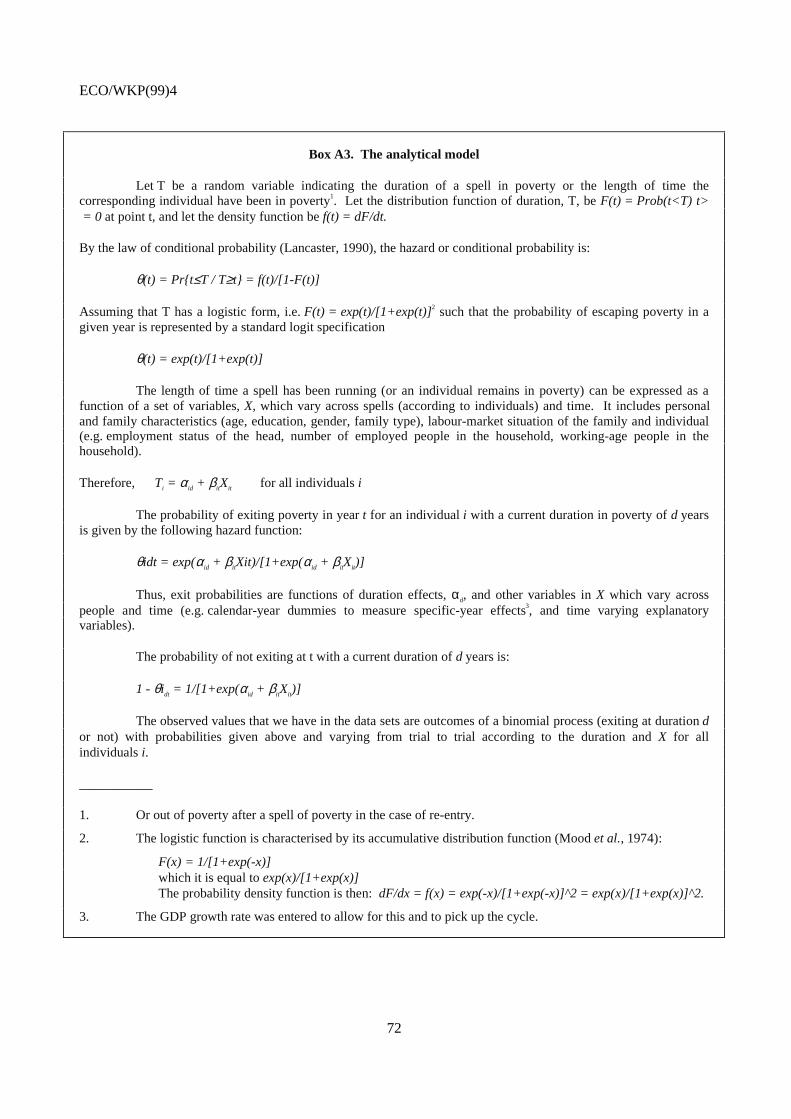
ECO/WKP(99)4

72

Box A3. The analytical model

Let T be a random variable indicating the duration of a spell in poverty or the length of time thecorresponding individual have been in poverty1. Let the distribution function of duration, T, be F(t) = Prob(t<T) t> = 0 at point t, and let the density function be f(t) = dF/dt.

By the law of conditional probability (Lancaster, 1990), the hazard or conditional probability is:

θ(t) = Pr{t≤T / T≥t} = f(t)/[1-F(t)]

Assuming that T has a logistic form, i.e. F(t) = exp(t)/[1+exp(t)]2 such that the probability of escaping poverty in agiven year is represented by a standard logit specification

θ(t) = exp(t)/[1+exp(t)]

The length of time a spell has been running (or an individual remains in poverty) can be expressed as afunction of a set of variables, X, which vary across spells (according to individuals) and time. It includes personaland family characteristics (age, education, gender, family type), labour-market situation of the family and individual(e.g. employment status of the head, number of employed people in the household, working-age people in thehousehold).

Therefore, Ti = αid + βitXit for all individuals i

The probability of exiting poverty in year t for an individual i with a current duration in poverty of d yearsis given by the following hazard function:

θidt = exp(αid + βitXit)/[1+exp(αid + βitXit)]

Thus, exit probabilities are functions of duration effects, αd, and other variables in X which vary acrosspeople and time (e.g. calendar-year dummies to measure specific-year effects3, and time varying explanatoryvariables).

The probability of not exiting at t with a current duration of d years is:

1 - θidt = 1/[1+exp(αid + βitXit)]

The observed values that we have in the data sets are outcomes of a binomial process (exiting at duration dor not) with probabilities given above and varying from trial to trial according to the duration and X for allindividuals i.

__________

1. Or out of poverty after a spell of poverty in the case of re-entry.

2. The logistic function is characterised by its accumulative distribution function (Mood et al., 1974):

F(x) = 1/[1+exp(-x)]which it is equal to exp(x)/[1+exp(x)]The probability density function is then: dF/dx = f(x) = exp(-x)/[1+exp(-x)]^2 = exp(x)/[1+exp(x)]^2.

3. The GDP growth rate was entered to allow for this and to pick up the cycle.

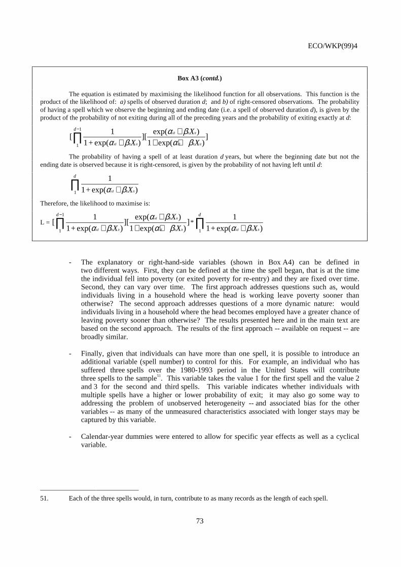
ECO/WKP(99)4

73

Box A3 (contd.)

The equation is estimated by maximising the likelihood function for all observations. This function is theproduct of the likelihood of: a) spells of observed duration d; and b) of right-censored observations. The probabilityof having a spell which we observe the beginning and ending date (i.e. a spell of observed duration d), is given by theproduct of the probability of not exiting during all of the preceding years and the probability of exiting exactly at d:

[ ][ ]1

11

1

1+ exp( )exp( )

exp( )α βα β

α βid it it

id it it

id it itX

X

X

d

++

+ +

−

∏The probability of having a spell of at least duration d years, but where the beginning date but not the

ending date is observed because it is right-censored, is given by the probability of not having left until d:

1

1 1+ exp( )α βid it itX

d

+∏Therefore, the likelihood to maximise is:

L = [ ][ ]1

11

1

1+ exp( )

exp( )

exp( )α βα β

α βid it it

id it it

id it itX

X

X

d

++

+ +

−

∏ *1

1 1+ exp( )α βid it itX

d

+∏

- The explanatory or right-hand-side variables (shown in Box A4) can be defined intwo different ways. First, they can be defined at the time the spell began, that is at the timethe individual fell into poverty (or exited poverty for re-entry) and they are fixed over time.Second, they can vary over time. The first approach addresses questions such as, wouldindividuals living in a household where the head is working leave poverty sooner thanotherwise? The second approach addresses questions of a more dynamic nature: wouldindividuals living in a household where the head becomes employed have a greater chance ofleaving poverty sooner than otherwise? The results presented here and in the main text arebased on the second approach. The results of the first approach -- available on request -- arebroadly similar.

- Finally, given that individuals can have more than one spell, it is possible to introduce anadditional variable (spell number) to control for this. For example, an individual who hassuffered three spells over the 1980-1993 period in the United States will contributethree spells to the sample51. This variable takes the value 1 for the first spell and the value 2and 3 for the second and third spells. This variable indicates whether individuals withmultiple spells have a higher or lower probability of exit; it may also go some way toaddressing the problem of unobserved heterogeneity -- and associated bias for the othervariables -- as many of the unmeasured characteristics associated with longer stays may becaptured by this variable.

- Calendar-year dummies were entered to allow for specific year effects as well as a cyclicalvariable.

51. Each of the three spells would, in turn, contribute to as many records as the length of each spell.

ECO/WKP(99)4

74

Box A4. Explanatory variables for estimates of the duration of poverty and re-entry

Age groups: <16, 16-24, 25-34, 35-49, 50-64, 65+

Education level: two variables are available, the level attained:

1. lower than high school,2. high school,3. higher than high school

and the number of years of formal education. Those individuals without stated education level, children, wereassigned the education level of the head of household.

Gender

Race: whether the individual was white or non-white (only in the United States)

Employment status: whether the individual was employed or not

Household composition: number of adultsnumber of children in the householdnumber of adults working

Family type: single adult (head) with no childrensingle adult (head) with childrentwo or more adults with no childrentwo or more adults with children

100. An additional test was performed in which the available sample was broken into two parts. Thesecond part of the sample was used to estimate the probability of exiting poverty conditional on duration.The first part was used to create a variable for previous spells of poverty. The results of this exerciseconfirm those presented in the tables at the end of this note that previous spells in poverty increase thelength of time in poverty or reduces the chances of earlier exit.

3.3. Comments on the explanatory variables and estimations

101. The explanatory variables presented in Box A4 were all defined for the individual and for thehead of his household. Therefore, an individual can be associated with his own personal characteristics(e.g. age, education, gender), and those related to the household (s)he belongs to (e.g. household type, thenumber of children in the household and the number of workers in the household), and those associated tothe head of the household (e.g. education, age, gender of the head, health status of the head, employmentstatus of the head).

102. Furthermore, each individual is associated with a variable that counts the number of spells inpoverty and dummy variables that account for the duration of the spell and year dummies or calendaryears. In final specifications, the GDP growth rate replaced the year dummies.

103. The variables related to age and education were introduced in the estimation process as eitherdummies controlling for individual characteristics or as dummies controlling for the age and educationallevel of the household head. The results are similar for both specifications. The estimated equationsreported below (Tables A7 and A8) use the age, gender and educational level of the individual.

ECO/WKP(99)4

75

104. The factors that explain duration persistence and re-entry appear quite similar across countries.The employment status of the household seems to be the main factor leading to shorter poverty spells. Thenumber of adults working in the household as well as the employment status of the household head(i.e. whether the head of the household is employed or not) are highly significant.

105. Belonging to a lone-parent household appears to be one of the most important factor leading tolonger spells52. The dummy variable controlling for single-adult households with children was interactedwith the gender of the head. The results presented below only show this variable without its interaction,but other estimated results -- available on request -- show that the negative effect of lone parents iscompletely due to female lone parents in all three countries. This confirms the commonly found result forthe United States that individuals in female-headed households and, in particular, those with children aremore prone to remain in poverty for long periods. The equations also confirm that the non-whitepopulation in the United States stays longer in poverty.

106. Variables indicating the age of the individual do not appear significant. In particular, there is noevidence that children, taken as a group, appear to stay longer in poverty. Education (except for the UnitedStates) does not appear to affect the length of poverty spells. Health status also appears significant only inthe United States, where is a measure of disability instead of self-reported health as in Germany and theUnited Kingdom. However, both education and poor health status appear to affect the re-entry intopoverty (following an exit) in all three countries.

107. The results for Canada, while confirming the importance of employment to reduce povertypersistence, differ slightly from the results of the other three countries. The main distinction is that certaingroups (e.g. lone parents and people with previous poverty experience) which are in disadvantage in theother three countries are not so in Canada. And old age people seem to fare much better in Canada.

52. The estimated results reported for the United Kingdom for lone parent households are not statistically

significant. When using the more appropriate monthly measure of household income in the BHPS, loneparent households are worst off than other households.

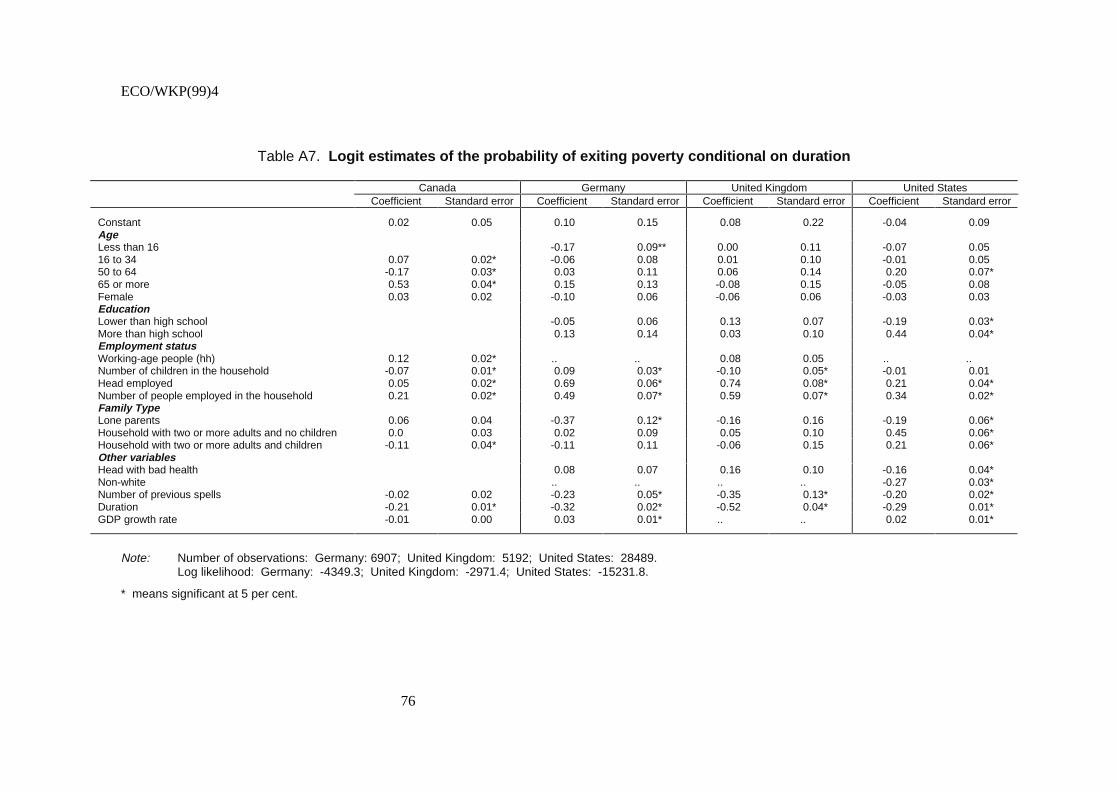
ECO/WKP(99)4

76

Table A7. Logit estimates of the probability of exiting poverty conditional on duration

Canada Germany United Kingdom United StatesCoefficient Standard error Coefficient Standard error Coefficient Standard error Coefficient Standard error

Constant 0.02 0.05 0.10 0.15 0.08 0.22 -0.04 0.09AgeLess than 16 -0.17 0.09** 0.00 0.11 -0.07 0.0516 to 34 0.07 0.02* -0.06 0.08 0.01 0.10 -0.01 0.0550 to 64 -0.17 0.03* 0.03 0.11 0.06 0.14 0.20 0.07*65 or more 0.53 0.04* 0.15 0.13 -0.08 0.15 -0.05 0.08Female 0.03 0.02 -0.10 0.06 -0.06 0.06 -0.03 0.03EducationLower than high school -0.05 0.06 0.13 0.07 -0.19 0.03*More than high school 0.13 0.14 0.03 0.10 0.44 0.04*Employment statusWorking-age people (hh) 0.12 0.02* .. .. 0.08 0.05 .. ..Number of children in the household -0.07 0.01* 0.09 0.03* -0.10 0.05* -0.01 0.01Head employed 0.05 0.02* 0.69 0.06* 0.74 0.08* 0.21 0.04*Number of people employed in the household 0.21 0.02* 0.49 0.07* 0.59 0.07* 0.34 0.02*Family TypeLone parents 0.06 0.04 -0.37 0.12* -0.16 0.16 -0.19 0.06*Household with two or more adults and no children 0.0 0.03 0.02 0.09 0.05 0.10 0.45 0.06*Household with two or more adults and children -0.11 0.04* -0.11 0.11 -0.06 0.15 0.21 0.06*Other variablesHead with bad health 0.08 0.07 0.16 0.10 -0.16 0.04*Non-white .. .. .. .. -0.27 0.03*Number of previous spells -0.02 0.02 -0.23 0.05* -0.35 0.13* -0.20 0.02*Duration -0.21 0.01* -0.32 0.02* -0.52 0.04* -0.29 0.01*GDP growth rate -0.01 0.00 0.03 0.01* .. .. 0.02 0.01*

Note: Number of observations: Germany: 6907; United Kingdom: 5192; United States: 28489.Log likelihood: Germany: -4349.3; United Kingdom: -2971.4; United States: -15231.8.

* means significant at 5 per cent.

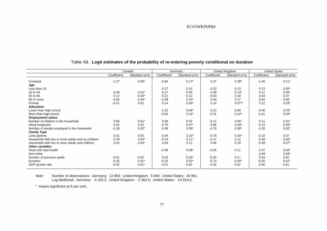
ECO/WKP(99)4

77

Table A8. Logit estimates of the probability of re-entering poverty conditional on duration

Canada Germany United Kingdom United StatesCoefficient Standard error Coefficient Standard error Coefficient Standard error Coefficient Standard error

Constant -1.27 0.05* -0.84 0.17* 0.37 0.28* -1.40 0.11*AgeLess than 16 0.17 0.10 0.23 0.13 0.13 0.05*16 to 34 -0.08 0.02* 0.17 0.09 0.39 0.13* 0.11 0.05*50 to 64 0.12 0.03* 0.21 0.12 -0.03 0.18 0.04 0.0765 or more -0.50 0.04* -0.38 0.15* 0.43 0.17 0.02 0.08Female -0.01 0.02 0.14 0.06* 0.14 0.07** 0.12 0.03*EducationLower than high school 0.15 0.06* 0.10 0.09 0.40 0.03*More than high school -0.63 0.15* -0.31 0.12* -0.41 0.04*Employment statusNumber of children in the household 0.06 0.01* 0.06 0.03 -0.11 0.05* 0.11 0.01*Head employed 0.02 0.02 -0.79 0.07* -0.86 0.09* -0.14 0.05*Number of people employed in the household -0.18 0.02* -0.48 0.06* -0.79 0.08* -0.25 0.02*Family TypeLone parents 0.01 0.05 0.44 0.15* 0.76 0.20* -0.10 0.07Household with two or more adults and no children 0.29 0.03* -0.24 0.11* -0.17 0.12 -0.40 0.06*Household with two or more adults and children 0.42 0.04* 0.05 0.12 0.06 0.18 -0.28 0.07*Other variablesHead with bad health -0.49 0.08* -0.05 0.11 0.37 0.04*Non-white .. .. .. .. 0.49 0.03*Number of previous spells -0.01 0.02 0.22 0.05* -0.20 0.17 0.03 0.02Duration -0.35 0.01* -0.25 0.02* -0.73 0.05* -0.25 0.01*GDP growth rate -0.02 0.01* 0.01 0.02 -0.03 0.02 0.00 0.01

Note: Number of observations: Germany: 13 850; United Kingdom: 5 840; United States: 34 851.Log likelihood: Germany: -4 325.2; United Kingdom: -2 363.6; United States: -14 914.6.

* means significant at 5 per cent .

ECO/WKP(99)4

78

ECONOMICS DEPARTMENTWORKING PAPERS

211. The Recent Experience with Capital Flows to Emerging Market Economies(February 1999) Sveinbjörn Blöndal and Hans Christiansen

210. Foreign Portfolio Investors Before and During a Crisis(February 1999) Woochan Kim and Shang-Jin Wei

209. Towards More Efficient Government : Reforming Federal Fiscal Relations in Germany(February 1999) Eckhard Wurzel

208. Stock Market Fluctuations and Consumption Behaviour : Some Recent Evidence(December 1998) Laurence Boone, Claude Giorno and Pete Richardson

207. Microeconometric analysis of the retirement decision: The Netherlands(June 1998) Maarten Lindeboom

206. Microeconometric analysis of the retirement decision: United Kingdom(June 1998) Raffaele Miniaci and Elena Stancanelli

205. Microeconometric analysis of the retirement decision: Italy(June 1998) Raffaele Miniaci

204. Microeconometric analysis of the retirement decision: Germany(June 1998) Pablo Antolin and Stefano Scarpetta

203. Microeconometric analysis of the retirement decision: United States(June 1998) Joseph Quinn, Richard Burkhauser, Kevin Cahill and Robert Weathers

202. The retirement decision in OECD countries(June 1998) Sveinbjörn Blöndal and Stefano Scarpetta

201. The macroeconomic effects of pension reforms in the context of ageing populations:overlapping generations model simulations for seven OECD countries(June 1998) Ketil Hviding and Marcel Mérette

200. The macroeconomics of ageing, pensions and savings: a survey(June 1998) Richard Kohl and Paul O’Brien

199. Marginal Effective Tax Rates on Physical, Human and R&D Capital (May 1998) Kathryn Gordon andHarry Tchilinguirian

198. The Norwegian Health Care System(May 1998) Paul van den Noord, Terje Hagen and Tor Iversen

197. APEC Trade Liberalisation : Its Implications(May 1998) Seunghee Han and Inkyo Cheong

196. The OECD Jobs Strategy : Progress Report on Implementation of Country Specific Recommendations(May 1998)

ECO/WKP(99)4

79

196 La Strategie de l’OCDE pour l’emploi : rapport sur l’état d’avancement de la mise en oeuvre des recommandations par pays(May 1998)

195. Trends in OECD Countries’ International Competitiveness(April 1998) Martine Durand, Christophe Madashi and Flavia Terribile

194. The European Union’s Trade Policies and their Economic Effects(April 1998) Peter Hoeller, Nathalie Girouard and Alessandra Colecchia

193. The Macroeconomic Implications of Ageing in a Global Context(March 1998) Dave Turner, Claude Giorno, Alain De Serres, Ann Vourc’h and Pete Richardson

192. Efficiency and Distribution in Computable Models of Carbon Emission Abatement(March 1998) Joaquim Oliveira Martins and Peter Sturm

191. Monetary Policy when Inflation is Low(March 1998) Charles Pigott and Hans Christiansen

190. Submission by the OECD to the G8 Growth, Employability and Inclusion Conference(March 1998)

189. Income Distribution and Poverty in Selected OECD Countries(March 1998) Jean-Marc Burniaux, Thai-Thanh Dang, Douglas Fore, Michael Förster,Marco Mira d’Ercole and Howard Oxley

188. Asset Prices and Monetary Policy(February 1998) Mike Kennedy, Angel Palerm, Charles Pigott and Flavia Terribile

187. NAIRU: Incomes Policy and Inflation(January 1998) Silvia Fabiani, Alberto Locarno, Gian Paolo Oneto and Paolo Sestito

186. OECD Submission to the Irish National Minimum Wage Commission(December 1997)

185. OECD Submission to the UK Low Pay Commission(December 1997)

184. Concept, Measurement and Policy Implications of the NAIRU - Perspective from Belgium(October 1997) Joost Verlinden

183. Structural unemployment in Denmark(September 1997) Agnete Gersing

182. The United Kingdom NAIRU: Concepts, Measurement and Policy Implications(September 1997) Chris Melliss and A.E. Webb

181. Globalisation and Linkages: Macro-Structural Challenges and Opportunities(August 1997) Pete Richardson

180. Regulation and Performance in the Distribution Sector(August 1997) Dirk Pilat

Poverty Dynamics in Four OECD Countries

Documents