Potential Diversification Benefits In The Presence Of Unknown Structural Breaks: An Australian Case Study

1

PACIFIC RIM REAL ESTATE SOCIETY CONFERENCE Christchurch, New Zealand

January, 2002, Potential Diversification Benefits in the Presence of Unknown Structural Breaks:

An Australian Case Study* Patrick J. Wilson** Richard Gerlach School of Finance and Economcs School of Mathematical and

Physical Sciences University of Technology, Sydney University of Newcastle

Ralf Zurbruegg School of Commerce University of Adelaide Abstract

It is reasonable to suggest that a portfolio manager with direct property diversified by sector or region is more interested in strategic than in tactical asset allocation. However, even with strategic allocations of property the portfolio manager needs a regular monitoring of the inter-relationships amongst assets comprising the portfolio to ensure that unexpected events do not `permanently’ alter such relationships. One procedure for ascertaining whether assets are inter-related over the long run (and therefore offer few diversification benefits) is through cointegration analysis. A difficulty with conventional cointegration analysis, however, is that it is unable to accommodate changes in equilibrium relationships amongst assets that might occur due to unexpected structural changes. In this paper we apply the Gregory and Hansen cointegrating procedure to consider how unexpected structural changes might affect the potential long run diversification benefits of assets held in an Australian property portfolio.

* We express our appreciation to the Property Council of Australia for making data available for this analysis

** Contact Author email: [email protected] fax: 61(0)295147711 phone: 61(0)295147777 address: PO Box 123, Broadway, NSW, Australia, 2001

2

Introduction Either or both sectoral and geographic diversification are generally considered as

suitable vehicles to obtain risk reduction benefits in either direct or indirect property

portfolios. Preliminary information on potential risk reduction is obtained through

examination of simple correlation structures. Recent research has suggested that, since

such correlation structures may be temporally unstable, the signals on appropriate

combinations of assets to join the portfolio may be difficult to interpret. Another means

by which preliminary information on asset combinations can be obtained is through use

of the cointegration framework. If assets in the same class, but held in two or more

distinct geographic regions, are cointegrated this would indicate that the markets are

trending together over the long run. Similarly, if assets in different property sub-classes

are cointegrated this would indicate that there are one or more common stochastic trends

in the assets. Under such circumstances there would only be limited (if any) opportunity

to gain risk reduction benefits through investing in the markets of both regions and/or

classes.

There are two broad approaches to testing for cointegrating relationships. One

approach is to pursue the Engle-Granger (1987) two -step methodology of applying unit

root tests to the residual series of a cointegration equation. An alternative procedure is to

apply the Johansen (1991) procedure of testing for a cointegrating relationship in a

system of equations.

A potential difficulty in using the cointegration framework arises if one or more

of the asset series has been subjected to a structural break or regime shift1. Such change

may come about through relatively infrequent but important events such as changes to the

3

fiscal treatment of property either in different regions or sub-asset classes, differences in

the growth or decline of regional economies - perhaps brought about through the closure

of important employment industries (for instance closure of the steelworks in the

Newcastle region, downsizing of the steel industry in the Illawarra), and so on… . These

events alter the economic performance of regions with consequent flow through to

property asset holdings in those regions. Gregory, Nasson and Watt (1994) have shown

that conventional Engle-Granger cointegration tests do not perform well in the presence

of structural breaks in the series. In particular, they show that the power of a conventional

Augmented Dicky-Fuller (ADF) test fails in the presence of a structural break. That is, it

may be possible that two or more series are cointegrated with a one time shift in the

cointegrating vector, but a conventional ADF test on the residual series may fail to reveal

this cointegration. Thus, for example, if a property portfolio manager applied a

conventional Engle-Granger methodology to property asset series in two different states

or regions or across two property sub-classes and found that these property assets were

not cointegrated then, ceteris paribus, the manager may decide to add each of the

property assets to the portfolio. However, it may be that the existence of an unknown

(and unaccounted for) structural break in the cointegrating vector yielded the result of no

cointegration. If it turned out that the series were, in fact, cointegrated then the portfolio

may fail to attract the expected risk reduction benefits through diversifying across states

or asset sub-classes. In this paper we will apply the cointegration methodology to several

property portfolios constructed from assets in different Australian states to determine

whether there is a long run equilibrium relationship amongst these assets. We will adopt

two approaches. In the first instance we will apply the Johansen (1991) methodology to

4

ascertain whether there appears to be evidence of cointegration amongst the groups of

assets held in each portfolio. We will then apply the Gregory and Hansen (1996)

procedure on bivariate asset series within each portfolio to ascertain whether there

appears to be evidence of cointegration in the presence of a possible structural break in

either or both of the series of interest. The remainder of the paper is as follows: in

section two we briefly review the literature on geographic diversification; section three

presents a statement on the cointegration methodology; in section four we discuss data

sources and present the results while section five offers some conclusions.

Section Two: Some Previous Research

While it is reasonable to argue that national economic performance has a strong

influence on real estate markets in general it is also reasonable to suppose that local

market conditions also have an important bearing. To the extent that this is true,

therefore, a portfolio of geographically diverse properties may provide better risk return

characteristics than a geographically concentrated portfolio. To examine this notion in

the past decade or so several researchers have looked at the potential risk reduction

benefits to accrue through geographic diversification of property holdings. A majority of

this research has commenced with a study of correlation structures as a means of

providing preliminary information on potential portfolios which are then examined for

risk-return performance. For instance Mueller and Ziering (1992) and Mueller (1993)

examined the real estate diversification benefits of categorizing local economies by

`dominant industry’ rather than by political boundary and found that real estate portfolios

constructed of regions based on `economic’ characteristic were more efficient. In a

5

broader context Eichholtz and Lie (1995) found that there were increasing correlations

among real estate markets within continents and decreasing correlations between

continents, implying a fall in risk reduction benefits from portfolios constructed on a

regional basis but improved benefits from globally constructed portfolios. However,

correlation analysis is not the only procedure available for initial asset selection. Tarbert

(1998) has raised concern over the dangers of using conventional correlation techniques

in preliminary portfolio construction due to the temporal instability of such correlations,

pointing to earlier work on this by Baum and Schofield (1991). The main difficulty

revolves around the idea that, since correlation coefficients are temporally unstable, a

well diversified portfolio initially selected through correlation analysis in one period may

not hold in subsequent periods. In a move away from correlation analysis Tarbert (1998)

applied cointegration techniques for initial property portfolio selection and found that the

potential risk reduction benefits of property diversification by region and sector within

the UK were more limited than earlier research by Eichholtz et.al. (1994) had indicated.

Informal graphical tests can be conducted to assess the temporal stability of the

relationship between any two asset series. This can be done via rolling correlations,

measuring the association between groups of, say, 20 paired observations. The window is

moved forward one point at a time and the correlation is measured again using the last 20

paired data points. These correlations will be highly dependent on e ach other but can give

a graphical assessment of whether relationships are changing over time. Any notions of

temporal instability in correlations are then examined by looking at the changes in

correlation structure as the sample is rolled through the series. Further, it is

straightforward to conduct Monte Carlo tests using the series of correlations obtained to

6

assess whether changes have occurred just via natural variation or whether a shift in the

relationship may have occurred.

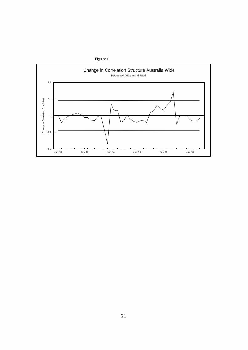
For example, figure 1 plots the change in correlation structure for a rolling

correlation between the price returns series for All Office and All Retail (described

below) for Australia. The dark heavy lines are 95% confidence intervals for the

difference in correlations (obtained by simulation and accounting for the variability in the

data and the dependence in the rolling correlations) if the data are normal and the

correlation between them is stable at the value of the sample correlation when using all

the data (in this case the full sample correlation is 0.44 while the rolling values range

from -.21 to +0.82)2. From figure 1 it is evident that the relationship between the series

appears to shift around significantly about the mid nineties and again in the late nineties

as it crosses the 95% lines on several occasions.

Section Three: The Cointegration Approach

If two or more property series are cointegrated then this implies that the

series are tied together by some common factor or factors and hence the series will not

drift too far apart over the long run. If the series in question happen to be assets held in

the same portfolio then the fact that these will behave in a similar fashion over the long

run implies reduced, or even no, diversification benefits through holding all of these

assets simultaneously. It is an important consideration, therefore, for the portfolio

manager to ascertain whether there is a cointegrating relationship between/amongst assets

held in the portfolio. A preliminary step in testing for cointegration is to determine

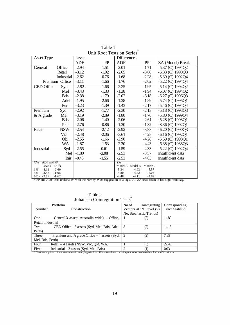
whether the series are integrated to the same order. Table 1 presents the outcome from

7

conventional Augmented Dicky-Fuller (ADF) and Phillips-Perron (PP) unit root tests.

However, a difficulty with these conventional unit root tests is that they lack power in the

presence of potential structural breaks in the series – for instance the tests may fail to

indicate whether a series is first difference stationary. Several tests have been developed

to ascertain whether a series has a unit root in the presence of potential structural breaks,

the most popular of which is that by Zivot and Andrews (1992). The Zivot and Andrews

(ZA) methodology followed Perron (1989) in considering three possible types of

structural break in a series viz. models A (a ‘crash’ model with no change in growth), B

(change in growth, but no change in level), and C (the most general model permitting

both occurrences). The ZA models test for stationarity subject to structural breaks in the

series. The dummy variable DU t accommodates a one-time level shift in the series and

DTt a one time trend shift. The breakfraction locates each potential break in the series

and is the number of observations up to each breakpoint TB as a proportion of the total

sample ( T). For example, in the most general model (model C) the breakpoint DUt is

chosen as the minimum t-value on α for sequential tests of the breakpoint occurring at

time 1<TB<T3:

Equation 1

eyc+y+ )TD(d +DT + t+ DU+=y tj)( tj

k

1=j1-ttB

*ttt + ˆˆˆˆˆˆˆˆ −∆Σαγβθµ

where D(TB) t = 1 if t=TB+1, 0 otherwise; DU t =1 if t>TB, 0 otherwise and DT*

t = t -TB

and DT t = t if t>TB and 0 otherwise. Because the Zivot-Andrews methodology is not

conditional on the prior selection of the breakpoint the critical values are larger (in an

absolute sense) than the conventional ADF critical values, consequently it is more

difficult to reject the null hypothesis of a unit root. Our procedure was to apply the most

8

general test (model C) in the first instance. If that test indicated the series was stationary

in first differences the testing ceased (i.e. we did not move forward to consider all

possible breaks). If model C was inconclusive we moved to test the more restricted

models B and A.

The results of this procedure are also shown in table 1. Here we see that

conventional ADF and PP tests indicated that most series were I(1) but in those cases no t

so indicated we see that once the broader ZA tests were applied all series are shown to be

I(1).

Since all series are I(1) there is a suitable environment in which to test for the

existence of long run equilibrium relationhips amongst the assets. In the first instance a

standard Johansen (1991, 1995) cointegration test is conducted. The general

autoregressive representation for the vector Y, which contains v assets (series), all of

which are I(1)4, can be expressed as:

iit

k

iit YcY επ ++= −

=∑

1

Equation 2

where c is a constant term and πi is a v x v matrix of parameters. The maximum lag of the

system, k, is chosen so as to ensure that the residuals, εt, are white noise. This vector

autoregression system may also be re-arranged to yield an error correction model (ECM)

representation:

9

iktit

k

iit YYcY ε+Π+∆Γ+=∆ −−

−

=∑

1

1

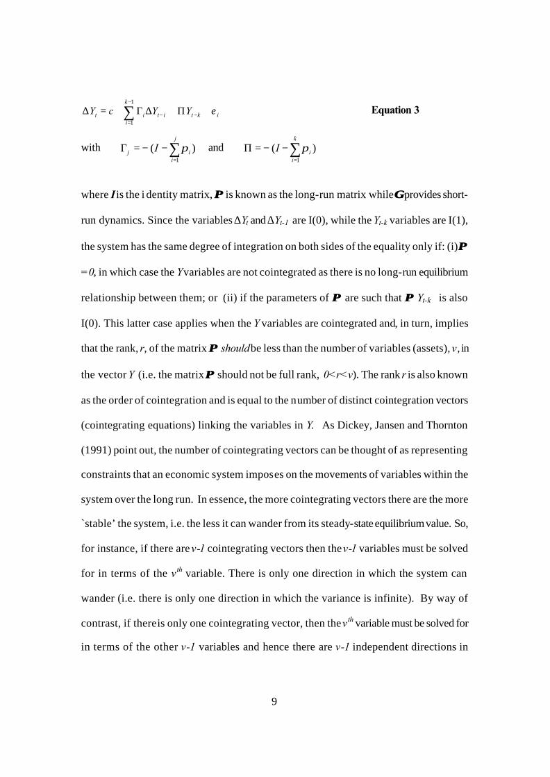
Equation 3

with )(1

∑=

−−=Γj

iij I π and )(

1∑

=

−−=Πk

iiI π

where I is the i dentity matrix, ΠΠ is known as the long-run matrix while ΓΓ provides short-

run dynamics. Since the variables ∆Yt and ∆Yt-1 are I(0), while the Yt-k variables are I(1),

the system has the same degree of integration on both sides of the equality only if: (i) ΠΠ

=0, in which case the Y variables are not cointegrated as there is no long-run equilibrium

relationship between them; or (ii) if the parameters of ΠΠ are such that ΠΠ Yt-k is also

I(0). This latter case applies when the Y variables are cointegrated and, in turn, implies

that the rank, r, of the matrix ΠΠ should be less than the number of variables (assets), v, in

the vector Y (i.e. the matrix ΠΠ should not be full rank, 0<r<v). The rank r is also known

as the order of cointegration and is equal to the number of distinct cointegration vectors

(cointegrating equations) linking the variables in Y. As Dickey, Jansen and Thornton

(1991) point out, the number of cointegrating vectors can be thought of as representing

constraints that an economic system imposes on the movements of variables within the

system over the long run. In essence, the more cointegrating vectors there are the more

`stable’ the system, i.e. the less it can wander from its steady-state equilibrium value. So,

for instance, if there are v-1 cointegrating vectors then the v-1 variables must be solved

for in terms of the vth variable. There is only one direction in which the system can

wander (i.e. there is only one direction in which the variance is infinite). By way of

contrast, if there is only one cointegrating vector, then the vth variable must be solved for

in terms of the other v-1 variables and hence there are v-1 independent directions in

10

which the system can wander – it is stable in only one direction. So, the fewer the

number of cointegrating vectors, the less constrained is the long-run relationship and the

more directions in which the system can wander from its steady state equilibrium value.

A portfolio manager would want to find as few as possible cointegrating vectors amongs t

the assets comprising the portfolio since the larger the number of cointegrating vectors

the less opportunity exists for risk reduction through diversification.

A potential drawback in applying the above test is that the outcome may be biased

if a struc tural break exists in the series. As Inoue (1999) points out, if a break exists then

a conventional testing procedure may mislead the analyst into either accepting the null of

no cointegration (in the case of a conventional Engle-Granger test) or the null of a

cointegrating rank smaller than the true rank (in the case of Johansen’s test).

One solution to this problem has been put forward by Gregory and Hansen (1996).

Gregory and Hansen (henceforth GH) devised a methodology for determining

cointegration in the presence of a single regime-shift. Specifically, they view their

technique as an extension of the univariate ZA test, which Fountas and Wu (1999) have

shown to be synonymous to a cointegration test with a prior restriction of the value of

one being placed on the cointegration parameter. However the GH test is more flexible

since the cointegration parameter is estimated and is not restricted to a value of one.

Here, as with the conventional Engle and Granger cointegration test (undertaken below

for comparative purposes), the null hypothesis is of no cointegration. However, this is

tested against the alternative hypothesis of cointegration with a regime shift. This allows

the researcher to test whether cointegration holds over some long period of time, but then

shifts to a new long run equilibrium relationship. Gregory and Hansen present three

11

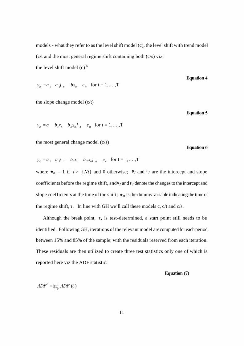
models - what they refer to as the level shift model (c), the level shift with trend model

(c/t and the most general regime shift containing both (c/s) viz:

the level shift model (c) 5

Equation 4

ττττ εβϕαα tttt xy +++= 21 for t = 1,….,T the slope change model (c/t)

Equation 5

τττττ εϕββα ttttt xxy +++= 21 for t = 1,….,T the most general change model (c/s)

Equation 6

ττττττ εϕββϕαα tttttt xxy ++++= 2121 for t = 1,….,T where jtτ = 1 if t > {Nτ} and 0 otherwise; a1 and b1 are the intercept and slope

coefficients before the regime shift, and a2 and b2 denote the changes to the intercept and

slope coefficients at the time of the shift; jtτ is the dummy variable indicating the time of

the regime shift, τ. In line with GH we’ll call these models c, c/t and c/s.

Although the break point, τ, is test-determined, a start point still needs to be

identified. Following GH, iterations of the relevant model are computed for each period

between 15% and 85% of the sample, with the residuals reserved from each iteration.

These residuals are then utilized to create three test statistics only one of which is

reported here viz the ADF statistic:

Equation (7)

)(inf* ττ

ADFADFT∈

=

12

where T is any compact subset (0,1), although in our case T = (0.15, 0.85).

Section Four: Data and Results

Data on direct property series was obtained from the Property Council of

Australia (PCA). To avoid the possibility that inflation may be a cointegrating factor in

the series all were CPI adjusted. The data used were also GST adjusted i.e. the one-off

effect of the GST was `stripped out’ and all data were changed to a December, 1994

base6. The PCA data series changed frequency from twice yearly to quarterly from June,

1995. This was dealt with by increasing the frequency for early periods using a linear

last match method. This uses a simple linear growth to generate an observation for the

missing quarter. The pr ocedure was deemed acceptable as it does not change the nature

of the relationship between the variables since each variable is treated the same.

Table 2 presents the outcome from the Johansen cointegration tests applied to

several different portfolios. Column one indicates the portfolio and the number of

assets making up the portfolio. So, for instance, the General portfolio holds office,

retail and industrial assets Australia wide. Column two shows the number of

cointegrating equations at the 5% level along with the number of common stochastic

trends in brackets, while column three indicates the corresponding trace statistic. The

first, and most general observation that we can make is that the Johansen test indicates

some degree of cointegration within every portfolio of property assets. The most

constrained portfolio, and hence the one likely to offer the fewest (if any) benefits over

the long run from geographic diversification, is the portfolio holding industrial property

in each capital city. Although industrial activity is primarily driven by the state of

the economy, and while the three cities represented lie on the eastern seaboard – i.e.

13

the most industrialized part of the country - the outcome from the test is not entirely

expected since one would anticipate local factors and local input by state governments

(tax concessions etc) to play an influencing role in bringing some divergence to industrial

activity. On the other hand the outcome may well be explained by the relatively small

number of observations on a city by city basis – the constraint being set by Melbourne

with 26 observations.

On the basis of the Johansen procedure the portfolio having the greatest potential

risk reduction benefit is retail holdings spread across the four main states. Retail sales

are less influenced by the state of the economy than other areas (motor vehicles, housing

etc.) but would certainly be influenced by local demographic factors (population

movements in search of employment, lifestyle and so on… ) so it seems reasonable to

expect more divergence of movement in retail property over the long term.

The apparent strength of the long run relationship amongst the office markets

spread over the capital cities is not surprising – either premium grade or general CBD

office. Banking, general finance and insurance are the main users of office space and

these industries tend to be driven by similar factors and hence one might expect similar

general movements in the asset prices, with some tempering due to local conditions.

The broad outcome from the analysis so far is that, while there may exist some

risk reduction benefits through geographic (and sectoral) diversification in Australian

property portfolios, it is clear that managers may need much greater consideration of the

long run implications of their investment choices.

From our earlier discussion it is evident that the complete story on long run

equilibrium relationships cannot be presented without consideration of potential breaks in

14

cointegrating relationships (and subsequent formation of new long run equilibrium

relationships). So, lets consider these same portfolio choices in the presence of potential

changes (breaks) in the cointegrating relationship. If both the Johansen tests and the GH

tests present outcomes suggesting a long run equilibrium relationship then this is strong

evidence of the existence of such a relationship, and some care is clearly needed in the

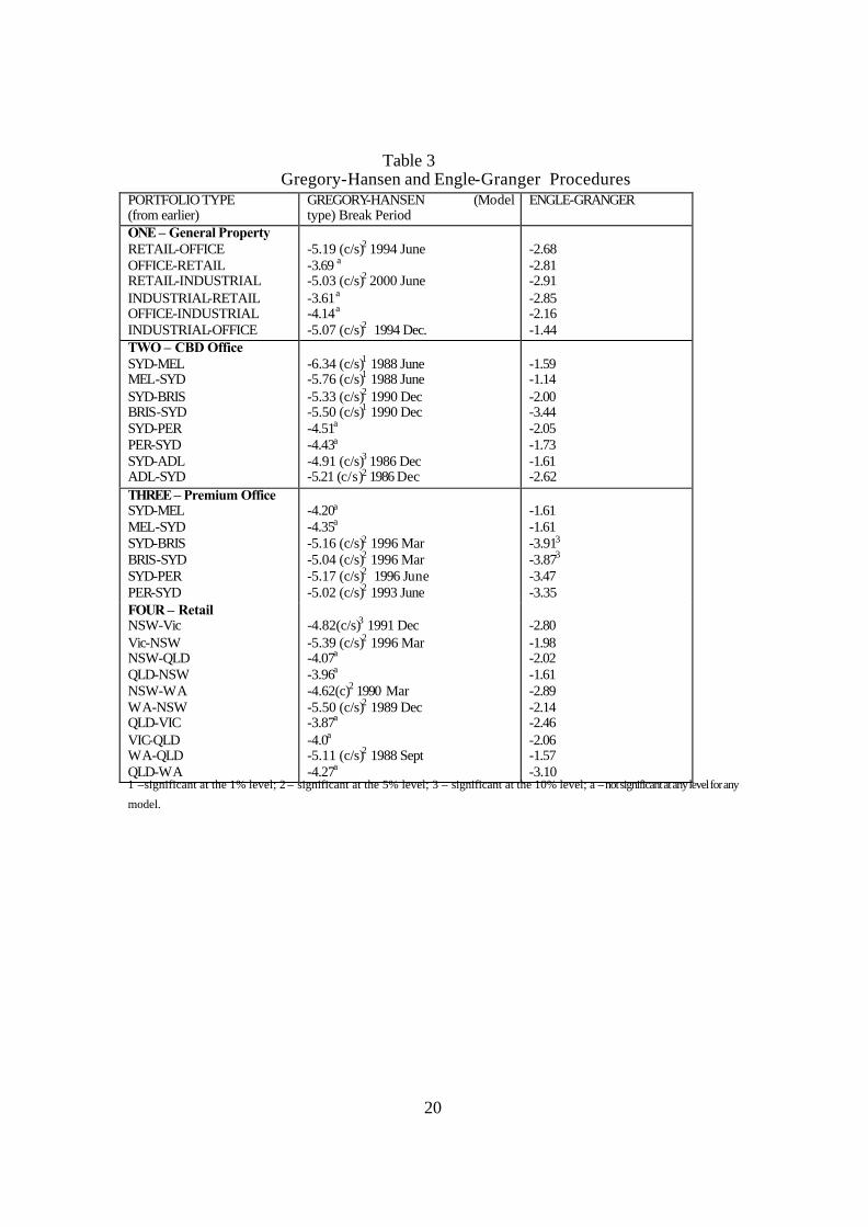
construction of a portfolio containing such cointegrated assets. Table 3 presents the GH

tests within each portfolio discussed above (along with conventional Engle-Granger ADF

tests for comparative purposes). The strategy here is twofold. In the first instance only

the most general GH model (c/s) is tested. If the outcome suggests cointegration (with a

change in the cointegrating relationship at the indicated date) then the analysis ceases. If

no cointegration is indicated then the c/t model is pursued, followed then by the c model.

This is a reasonable strategy since the only purpose here is to discover whether there

appear to be long run relationships (in the presence of unspecified change) amongst the

assets held in the portfolio. The second part of the strategy is to only pursue the tests on a

bivariate basis since the aim is to specifically identify those assets within the portfolio

that have a long run relationship. To reduce the size of the table the following practice is

adopted: if the portfolio contains more than three assets the assumption is made that,

since Sydney/NSW is the premier city and NSW the premier state (not only historically

but in terms of economic indicators) then managers may prefer to hold the relevant

assets from this city/state as a base for the portfolio. Hence the bivariate analysis is

restricted to Sydney/NSW along with consideration of the other assets. Since the

smallest value of the ADF test statistic is required to identify a rejection of the null

hypothesis, table 3 lists this along with the m odel type and the break point, τ. In the table

15

significant values are indicated and are based upon the asymptotic critical values given

by Gregory and Hansen (1996) (while significant values for the Engle-Granger tests are

those from McKinnon (1991). Like the ZA test the GH test considers each possible

point in the series as a potential break candidate and sequentially tests each point with the

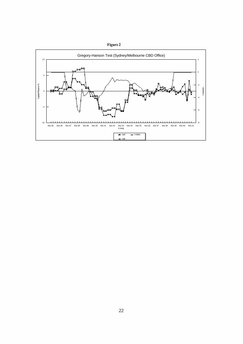
lowest ADF t-value emerging as the chosen period. In figure two we present a visual

impression of one such test for a possible cointegrating relationship between the Sydney

and Melbourne office markets. In this instance the GH general model suggests that the

markets are cointegrated and that a change in the cointegrating relationship occurred

about mid-1988.

Portfolio one is a general sectoral portfolio comprising office, retail and industrial

holdings Australia wide. From table 2 we know that Johansen suggested one

cointegrating vector. In table 3 conventional Engle-Granger results show that

irrespective of wh ich asset is considered the ̀ driver’ there is no cointegrating relationship

between any pair of assets. On the other hand the GH results indicate firstly that those

factors driving office and industrial markets will also have an influence on retail property,

but not vice-versa. This appears reasonable. The office and industrial sectors of the

economy are far more dependent on general economic conditions than retail markets and

this would have flow through effects to space users. While retail is less sus ceptible to

general movements in the economy it does not mean that this sector is not susceptible at

all, hence it seems reasonable to suppose that in a model which carries office and

industrial on the RHS there would be flow through effects. On the other hand the retail

sector is less driven by general economic conditions, therefore when retail is treated as a

RHS variable there may well be few flow through effects to the other sectors since retail

16

will not move as much with changes in the economy. This raises serious questions on the

proportions of each of these assets that should be held.

Portfolio two contains CBD office space in each of the capital cities. Table 2

showed that there was very little scope for independent movement amongst assets in the

portfolio (two common stochastic trends) while again the conventional Engle-Granger

test indicates no paired cointegrating relationship, implying that all of these assets could

potentially be held in the same portfolio. However, once the possibility of a structural

break in the cointegrating relationship is accounted for a very different picture emerges.

First, the results support Johansen and indicate that there may be very reduced benefits

from holding the eastern seaboard office assets in the same portfolio since, for each pair

of such assets there is a significant cointegrating relationship. By way of contrast, while

all eastern seaboard with other bivariate combinations were not considered, there is

evidence to indicate that some such asset combinations may possess long run

diversification benefits. In other words, while similar factors appear to drive the eastern

seaboard office markets these same factors may be less influential in driving other office

markets. For example, there is no cointegrat ing relationship when Sydney office is

combined with Perth office.

The portfolio of premium office space presents a somewhat mixed result

compared with the general CBD office portfolio. The Johansen results in table 2 have

already indicated a tendency for some of these assets to trend together over the long run

(two cointegrating vectors amongst the four assets). In table 3 both the GH test and the

conventional Engle-Granger approach suggest that only Sydney and Melbourne do not

have a cointegrating relationship. On the other hand, the combinations of holding

17

Sydney premium office with each of the other cities may be inadvisable since a

cointegrating relationship does exist, with a change in the nature of the relationship at the

indicated date, mostly mid 1996. In addition, even the Engle-Granger test supported

this outcome in the case of Sydney and Brisbane.

The Johansen test suggested that the retail portfolio possessed the greatest

potential for diversification benefits in own class asset holdings with three common

stochastic trends amongst the four assets and this outcome is certainly supported by the

Engle-Granger results in table 3 which indicate no cointegrating relationships. However

this picture changes somewhat once the possibility of breaks are taken into account. For

example, there are cointegrating relationships between retail assets in NSW and both

Victoria and Western Australia. Similarly there is a cointegrating relationship between

retail assets in Western Australia and Queensland (here we have expanded our ̀ rule’ of

anchoring the portfolio with NSW). So, while the potential still exists for geographical

diversification in retail holdings the picture does not appear quite as rosy as the outcomes

from the Johansen and Engle-Granger tests indicated.

Summary and Conclusion

Other research had expressed concern that since correlation structures are

temporally unstable the use of correlation for initial asset selection for a property

portfolio maybe inadvisable. In the present paper a brief example of such instability for

Australian real estate was presented to support this notion. Under such circumstances it

was suggested that it may be unwise to construct diversified portfolios on the basis of

changing correlation structures. Since investors in direct property are likely to take a

18

long view other research suggested that an alternative approach to initial asset selection

may be to use the cointegration methodology. However, in the presence of structural

breaks conventional cointegration methodology may not present a true indication of the

potential existence of long run relationships. Under such circumstances property

portfolios initially constructed on the basis of selection criteria using cointegration

analysis may not contain the diversification benefits at first thought. This was shown to

be the case in Australia where, using a cointegration methodology that accounts for

structural breaks, it was seen that portfolios of property assets diversified by region or

sector are likely to be smaller (contain fewer assets) than may have been previously

assumed to be appropriate.

19

Table 1 Unit Root Tests on Series* Asset Type Levels

ADF PP Differences ADF PP

ZA (Model) Break

General Office Retail Industrial Premium Office

-2.94 -1.51 -3.12 -1.92 -2.62 -0.76 -3.11 -1.66

-2.01 -1.71 -2.65 -3.60 -1.68 -2.28 -1.76 -2.02

-5.37 (C) 1994Q2 -6.33 (C) 1990Q3 -5.39 (C) 1992Q4 -5.22 (C) 1994Q4

CBD Office Syd Mel Bris Adel Per

-2.92 -1.66 -3.43 -1.33 -2.38 -1.79 -1.95 -2.66 -3.23 -1.39

-2.25 -1.95 -1.38 -1.94 -2.02 -3.18 -1.38 -1.89 -1.43 -2.17

-5.14 (C) 1994Q2 -6.07 (C) 1994Q2 -6.27 (C) 1996Q3 -5.74 (C) 1995Q1 -5.46 (C) 1994Q4

Premium Syd & A grade Mel Bris Per

-2.92 -1.77 -3.19 -2.89 -2.06 -1.40 -2.76 -0.86

-2.30 -2.13 -1.80 -1.76 -2.06 -2.61 -1.30 -1.82

-5.18 (C) 1993Q3 -5.80 (C) 1999Q4 -5.28 (C) 1993Q1 -8.36 (C) 1992Q1

Retail NSW Vic Qld WA

-2.54 -2.12 -2.48 -2.06 -2.55 -1.66 -1.87 -1.53

-2.92 -3.83 -3.61 -4.25 -2.90 -4.28 -2.30 -4.43

-6.20 (C) 1990Q3 -6.16 (C) 1992Q1 -5.59 (C) 1998Q1 -6.38 (C) 1988Q3

Industrial Syd Mel Bris

-2.55 -0.61 -1.80 -2.08 -0.43 -1.55

-1.59 -2.33 -2.53 -3.57 -2.53 -4.83

-5.22 (C) 1992Q4 insufficient data insufficient data

CVs ADF and PP Levels Diffs 1% -4.11 -2.60 5% -3.48 -1.95 10% -3.17 -1.62

ZA Model A Model B Model C -5.34 -4.93 -5.57 -4.80 -4.42 -5.08 -4.48 -4.11 -4.82

* PP and ADF tests undertaken with the Newey-West suggestion of 3 lags. All ZA tests taken to last significant lag.

Table 2 Johansen Cointegration Tests* Portfolio Number Construction

No.of Cointegrating Vectors at 5% level (vs No. Stochastic Trends)

Corresponding Trace Statistic

One General-3 assets Australia wide) – Office, Retail, Industrial

1 (2) 14.82

Two CBD Office –5 assets (Syd, Mel, Bris, Adel, Perth)

3 (2) 14.15

Three Premium and A grade Office – 4 assets (Syd, Mel, Bris, Perth)

2 (2) 7.65

Four Retail – 4 assets (NSW, Vic, Qld, WA) 1 (3) 22.49 Five Industrial – 3 assets (Syd, Mel, Bris) 2 (1) 0.03 * Test assumption: Linear deterministic trend; lags (in first differences) based on mid-point selection based on AIC and SC criteria.

20

Table 3 Gregory-Hansen and Engle-Granger Procedures PORTFOLIO TYPE (from earlier)

GREGORY-HANSEN (Model type) Break Period

ENGLE-GRANGER

ONE – General Property RETAIL-OFFICE OFFICE-RETAIL RETAIL-INDUSTRIAL INDUSTRIAL-RETAIL OFFICE-INDUSTRIAL INDUSTRIAL-OFFICE

-5.19 (c/s)2 1994 June -3.69 a -5.03 (c/s)2 2000 June -3.61 a -4.14 a -5.07 (c/s)2 1994 Dec.

-2.68 -2.81 -2.91 -2.85 -2.16 -1.44

TWO – CBD Office SYD-MEL MEL-SYD SYD-BRIS BRIS-SYD SYD-PER PER-SYD SYD-ADL ADL-SYD

-6.34 (c/s)1 1988 June -5.76 (c/s)1 1988 June -5.33 (c/s)2 1990 Dec -5.50 (c/s)1 1990 Dec -4.51a -4.43a -4.91 (c/s)3 1986 Dec -5.21 (c/s)2 1986 Dec

-1.59 -1.14 -2.00 -3.44 -2.05 -1.73 -1.61 -2.62

THREE – Premium Office SYD-MEL MEL-SYD SYD-BRIS BRIS-SYD SYD-PER PER-SYD

-4.20a -4.35a -5.16 (c/s)2 1996 Mar -5.04 (c/s)2 1996 Mar -5.17 (c/s)2 1996 June -5.02 (c/s)2 1993 June

-1.61 -1.61 -3.913 -3.873 -3.47 -3.35

FOUR – Retail NSW-Vic Vic-NSW NSW-QLD QLD-NSW NSW-WA WA-NSW QLD-VIC VIC-QLD WA-QLD QLD-WA

-4.82(c/s)3 1991 Dec -5.39 (c/s)2 1996 Mar -4.07a

-3.96a -4.62(c)2 1990 Mar -5.50 (c/s)2 1989 Dec -3.87a -4.0a -5.11 (c/s)2 1988 Sept -4.27a

-2.80 -1.98 -2.02 -1.61 -2.89 -2.14 -2.46 -2.06 -1.57 -3.10

1 –significant at the 1% level; 2 – significant at the 5% level; 3 – significant at the 10% level; a – not significant at any level for any

model.

21

Figure 1

-0.4

-0.2

0

0.2

0.4

Change in

Corr

ela

tion C

oeffic

ient

Jun-90 Jun-92 Jun-94 Jun-96 Jun-98 Jun-00

Change in Correlation Structure Australia WideBetween All Office and All Retail

22

Figure 2

-10

-5

0

5

10

-8

-6

-4

-2

0

2

X-Axis

Capita

l Retu

rns

%

t-st

atis

tic

Mar-85 Mar-86 Mar-87 Mar-88 Mar-89 Mar-90 Mar-91 Mar-92 Mar-93 Mar-94 Mar-95 Mar-96 Mar-97 Mar-98 Mar-99 Mar-00 Mar-01

syd

mel

t-value

Gregory-Hanson Test (Sydney/Melbourne CBD Office)

23

Bibliography

Baum, A.E. and Schofield, A (1991) “Property as a Global Asset” in Venmore-Rowland, P., Mole, T., Brandon, P.(eds.) Investment, Procurement and Performance in Construction, Chapman and Hall, 103-155. Dickey, David, Dennis W.Jansen and Daniel L. Thornton (1991) “A Primer on Cointegration with an Application to Money and Income”, Federal Reserve Bank of St.Louis Review, vol.73, no.2, March/April, 58-78. Eichholtz, Piet and Robert Lie (1995) “Globalisation of Real Estate Markets?” Eleventh Annual ARES Conference, Hilton Head Island Eichholtz, P, Hoesli, M., MacGregor, B.D. and Nanthakumaran, N. (1994) “Real Estate Portfolio Diversification: By Sector or Region?” ‘Cutting Edge’ Conference, City University Business School, published in RICS Proceedings , 343-384. Engle, R.F. and Granger, C.W.J. (1987) ‘Co-integration and Error Correction: Representation, Estimation, and Testing’, Econometrica, vol.55, 251 -276; Fountas, S. and J. Wu (1999) ‘Are the U.S. Current Account Deficits Really Sustainable?’, International Economic Journal , vol.13, no.3, 51-58. Gregory, A. and B. Hansen (1996) ‘Residual-Based tests for cointegration in models with regime shifts’, Journal of Econometrics, vol. 70, 99-126. Gregory, A.W., Nason, J.M. and D. Watt (1994), ‘Testing for structural breaks in cointegrated relationships’, Journal of Econometrics, vol.71, 321-341; Inoue, Atsushi (1999) “Tests of Cointegrating Rank with a Trend-break” Journal of Econometrics, vol.90, 215-237 Johansen, Soren (1995) Likelihood-based Inference in Cointegrated Vector Autoregressive Models , Oxford University Press, Oxford Johansen, S. (1991) ‘Estimation and Hypothesis Testing of Cointegration Vectors in Gaussian Vector Autoregressive Models,’ Econometrica, vol.59, 1551-1580. Mackinnon (1991) ‘Critical Values for Cointegration Tests’, Long-run Economic Relationships: Readings in Cointegration, 267-76, Oxford University Press. Mueller, Glenn R. and Barry A. Ziering, (1992) "Real Estate Portfolio Diversification Using Economic Diversification," Journal of Real Estate Research, , vol.7, no.4, 375-386.

24

Mueller, Glenn R, (1993) "Refining Economic Diversification Strategies For Real Estate Portfolios," Journal of Real Estate Research, vol.8, no.1, 55-68. Muscatelli, Vito Antonio and Stan Hurn (1995) “Econometric Modelling Using Cointegrated Time Series” in Oxley, Les et.al. Surveys in Econometrics, Blackwell, Oxford. Phillips, P (1987) ‘Time series regression with a unit root’, Econometrica, 55, 277-301. Perron, P. (1989) ‘The Great Crash, the Oil Price Shock, and the Unit Root Hypothesis’, Econometrica, vol.57, no.6, 1361-1401. Tarbert, Heather (1998) “The Long-run Diversification Benefits Available from Investing Across Geographical Regions and Property Type: Evidence from Cointegration Tests”, Economic Modelling, vol.15, 49-65 Zivot, E. and D. Andrews, (1992) ‘Further Evidence on the Great Crash, the Oil-Price Shock, and the Unit-Root Hypothesis’, Journal of Business and Economic Statistics, vol., 10, no.3, 251-70.

1 A structural break refers to a shift in the level and/or slope of a series. The Johansen test may be more robust than the Engle-Granger in the presence of a structural break 2 To account for variability we select the overall correlation, mean and variance between the two series and simulate 10,000 sets of observations of the same length with the equivalent correlation structure . For each of the 10,000 series we then undertake rolling correlations. 3 The more restricted models were: Model A

eyc+y + t+ )(DU+=y tj)( tAj

k

j=11-t

AAt

AAt + ˆˆˆˆˆˆˆ −∆Σαβλθµ

Model B

eyc+y + )(DT+t+=y tj)( tBj

k

j=11-t

B*t

BBBt + ˆˆˆˆˆˆˆ −∆Σαλγβµ

where the superscripts merely refer to models A and B and breakpoint indices etc. have the same interpretation as in the body of the paper. 4 Cf. Muscatelli and Hurn (1995) 5 Which Gregory and Hansen (1996a) specify both with and without trend. 6 The `stripping out’ effect was undertaken by the PCA