Potential Demand for Alternative Fuel Vehicles - EconStor

econstorMake Your Publications Visible.

A Service of

zbwLeibniz-InformationszentrumWirtschaftLeibniz Information Centrefor Economics

Dagsvik, John K.; Wetterwald, Dag G.; Aaberge, Rolf

Working Paper — Digitized Version

Potential Demand for Alternative Fuel Vehicles

Discussion Papers, No. 165

Provided in Cooperation with:Research Department, Statistics Norway, Oslo

Suggested Citation: Dagsvik, John K.; Wetterwald, Dag G.; Aaberge, Rolf (1996) : PotentialDemand for Alternative Fuel Vehicles, Discussion Papers, No. 165, Statistics Norway, ResearchDepartment, Oslo

This Version is available at:http://hdl.handle.net/10419/192149

Standard-Nutzungsbedingungen:

Die Dokumente auf EconStor dürfen zu eigenen wissenschaftlichenZwecken und zum Privatgebrauch gespeichert und kopiert werden.

Sie dürfen die Dokumente nicht für öffentliche oder kommerzielleZwecke vervielfältigen, öffentlich ausstellen, öffentlich zugänglichmachen, vertreiben oder anderweitig nutzen.

Sofern die Verfasser die Dokumente unter Open-Content-Lizenzen(insbesondere CC-Lizenzen) zur Verfügung gestellt haben sollten,gelten abweichend von diesen Nutzungsbedingungen die in der dortgenannten Lizenz gewährten Nutzungsrechte.

Terms of use:

Documents in EconStor may be saved and copied for yourpersonal and scholarly purposes.

You are not to copy documents for public or commercialpurposes, to exhibit the documents publicly, to make thempublicly available on the internet, or to distribute or otherwiseuse the documents in public.

If the documents have been made available under an OpenContent Licence (especially Creative Commons Licences), youmay exercise further usage rights as specified in the indicatedlicence.

www.econstor.eu

Discussion Papers No.165 • Statistics Norway, February 1996

John K. Dagsvik, Dag G. Wetterwaldand Rolf Aaberge

Potential Demand forAlternative Fuel Vehicles

Abstract:This paper analyzes the potential household demand for alternative fuel vehicles in Norway, by applyingdata from a stated preference survey. The alternative fuel vehicles we consider are liquid propane gasand electric powered vehicles in addition to a dual-fuel vehicle. In this survey each respondent, in arandomly selected sample, was exposed to 15 experiments. In each experiment the respondent is askedto rank three hypothetical vehicles characterized by specified attributes, according to the respondent'spreferences. Several versions of a random utility model are formulated and estimated. They include theordered logit model and a model with preferences that are correlated across experiments. The model isapplied to predict changes in demand resulting from price changes, and to assess the willingness to payfor alternative fuel vechicles.

Keywords: Stated preference, random utility, alternative fuel vehicles, ordered logit model, seriallydependent preferences.

JEL classification: C51, C93, D12.

Acknowledgement: We thank Tom Wennemo and René Wikestad for programming assistance andKari Anne Lysell for editing the paper.

Address: John K. Dagsvik, Statistics Norway, Research Department,P.O. Box 8131 Dep., N-0033 Oslo. E-mail: [email protected]

Rolf Aaberge, Statistics Norway, Research Department,P.O. Box 8131 Dep., N-0033 Oslo. E-mail: [email protected]

1 Introduction

In recent years the major automobile manufacturers have spent an increasing share of theirR&D expenditures to develop competitive alternatives to gasoline/diesel vehicles. Theseinclude different types of electric, hybrid, natural gas and multiple fuel vehicles. One obviousreason for this effort is the acknowledgement that the world's resources of oil is rather limited.Furthermore, there is increasing public awareness about the problems caused by pollutionfrom automobiles in many densely populated areas, and the fact that monoxide emissionfrom automobiles affects the world's ozone layers. A well known example of this is found insouthern California where air quality is an important concern. Here, the 1990 amendmentsto the Federal Clean Air Act and the 1990 Regulations by the California Air ResourcesBoard require substantial reduction in vehicle emissions.

This paper analyzes the potential household demand for alternative-fuel vehicles in Nor-way based on data from a stated preference type of survey conducted by Statistics Norway.

In stated preference surveys respondents are asked to express preferences for hypothetical

products characterized by specific attributes. Such experiments have some advantages over

market data. First, a detailed design of the new products can be presented to the consumersso as to obtain information about their attitudes towards new products and preferences over

product attributes. This is in contrast to the use of existing market data to forecast po-

tential demand which depends heavily on correct model specification and the requirement

that agents value attributes similarly for different products. Also, more information can be

elicited from a given agent in stated preference surveys since he/she can be asked to rank

the products in preference order. On the other hand, hypothetical choice situations can be

inferior to market data since the possibility of confusion or unstated assumptions cannot be

ruled out. Furthermore, one may also argue that individuals do not necessarily behave the

same way in laboratory experiments as they would in real markets with real products, since

they are not liable for their choices in hypothetical experiments. This issue is known as the

problem of external validity. Although academic research on external validity is rare, there

are, however, a few studies (cf. Levin et al. (1983) and Pearmain et al. (1991)) that indicate

considerable evidence of external validity. In the particular cases where the product under

investigation is not available in the market, the analyst has, however, no other choice but

to rely on hypothetical choice experiments.

So far, alternative fuel-vehicles have not been sufficiently developed to appear compet-

itive. For example, the battery technology of electric cars necessitate frequent recharging

and costly replacement. Thus, the shortcomings of current battery technology prevents

electric vehicles from being attractive in the market other than possibly for short/medium

range transportation purposes. An additional problem is that the current infrastructure on

maintenance and fuel supply is exclusively oriented towards conventional fuel vehicles, i.e.gasoline and diesel vehicles.

Although the data collected from the present stated preference survey yields some in-sight in individuals attitudes towards altenative fuel vechicles, it is nevertheless difficult

to get a clear picture of the structure of the preferences judging from summary statistics(from the survey) alone. One important reason for this is that the choice setting is rather

complicated with alternatives being characterized by several attributes which vary across

the experiments presented to the survey participants. Thus, summary statistics only reveals

"average behavior" across different experimental conditions. To fully analyze the structureof the preferences, it is therefore necessary to formulate and estimate a behavioral modelthat enables us to identify parameters of the distribution of the preferences. A further ad-

vantage with the behavioral modelling approach is that it can be applied to perform policy

experiments and to calculate compensating variation measures. Compensating variationmeasures are of interest to answer questions, such as: What are the respective amounts that

must be added to the purchase price of a specific alternative fuel vehicle to obtain the same

utility level, ceteris paribus, as the gasoline vehicle?

A major part of this paper is concerned with the formulation and estimation of several

versions of a structural model for individual choice behavior. The models discussed are

based on recent advances in the theory of discrete choice. The first version we discuss is

known as the ordered logit model. This model originates from the work of Luce (1959)

and Block and Marschak (1960), and has been applied to analyze potential demand for

electric vehicles by Beggs et al. (1981). In the ordered logit model it is assumed that the

decision-maker ranks the alternatives presented according to a random utility index where

the random components of the utility index are extreme value distributed and independent

across alternatives and across experiments (for a given individual). The second model we

discuss is an extension of the first one in that we allow the utility index for a given alternative

be dependent across experiments. The motivation for this extension is that there may be

memory or taste persistence effects implying that the decision-maker's preference evaluations

in successive experiments will be correlated. A version of this model was originally proposed

by Dagsvik (1983). In addition to these models we also discuss the ordered logit model with

random coefficients.In the context of studying the potential demand for alternative fuel vehicles, analyses

based on stated preference surveys are provided by Beggs et al. (1981), Hensher (1982) and

Calfee (1985), (these are electric vehicles), Bunch et al. (1991), Golob et al., (1991) andKitamura et al. (1991). See also Mannering and Train (1985) and Train (1980). In these

studies alternative fuel vehicle encompass electric, natural gas, liquid propane gas, hybrid

and other multiple fuel vehicles.

The organization of the paper is as follows: In the next section we describe the theoretical

point of departure and the rationale behind the chosen modeling framework. Section 3

discusses the survey method and provides a descriptive analysis of the data. In section 4 theempirical specification is presented and the estimation results are displayed and discussed.

Section 5 reports selected price elasticities and the distribution of compensating variation

for alternative fuel technologies.

4

2 Stochastic choice models

In the traditional (algebraic) theories for choice behavior under certainty the consumer(agent) is assumed to be perfectly rational, i.e., his preferences are deterministic and satisfya set of regularity and consistency conditions such as transitivity, continuity, etc. Thispoint of departure has a rather long tradition in economics, although an increasing body ofempirical evidence, as well as common daily life experience, suggest that agents often makedecisions under conflict in the sense that they have difficulty with assessing the precisevalue of each alternative. Furthermore, their preferences may change from one moment tothe next in a manner that is unpredictable (to the agents themselves).- In psychology, this

problem has long been recognized (cf. Tversky (1969)). Already Thurstone (1927) found

that often when individuals are exposed to the same choice experiment they tend to make

inconsistent choices. To account for this phenomenon, Thurstone introduced the (binary)

Thurstone random utility model. In this model the agent's preferences over alternatives

are represented by a normally distributed random utility function. This point of departure

seems particularly appealing in the context of analyzing potential demand for products

with which the consumers have little or no experience. There is by now a large literature on

probabilistic choice models, mainly developed by psychologists, where an important concern

is to provide a theoretical rationale for the structure of choice models consistent with the

notion of stochastic preferences (cf. Luce (1959), Luce et al. (1965), Luce (1977), Suppes

et al. (1989), McFadden, (1981)). In contrast, economists have mainly focused on problems

related to econometric specification and estimation of stochastic choice models and been

less concerned about theoretical foundation for the structure of this type of models.

A seminal contribution to the theory of probabilistic choice is Luce (1959) in which

he introduces his well known choice axiom; "independence from irrelevant alternatives"

(HA). The IIA assumption represents a stochastic formulation of rational behavior: While

the agent in each experiment is allowed to behave inconsistently, IIA states that when the

choice experiments are replicated a large number of times the agent will "on average" behave

consistently. The TJA property also implies a very tractable structure of the corresponding

choice model, often called the Luce model. This is also the case for choice experiments with

rankings, which is of particular relevance for the present study.

Based on empirical evidence the TJA assumption has often been critisized for being rather

restrictive. Apart from the "red bus-blue bus" example (cf. Debreu (1960)), the grounds for

rejecting TJA have, however, sometimes been somewhat superficially summarized. As is well

known but not always remembered, the TJA property may very well hold on the individual

level but fail to hold on "average" in a sample of heterogeneous agents where the observable

individual characteristics are insufficient for controlling properly for this heterogeneity.

5

2.1 Stochastic models for ranking

The systematic development of stochastic models for ranking started with Luce (1959) andBlock and Marschak (1960). Specifically, they provide a powerful theoretical rationale forthe structure of the so-called ordered logit model. The theoretical assumptions that underlythe ordered logit model can briefly be described as follows.

Let S denote the choice univers (i.e., the set of all alternatives) and let C c S be thechoice set of feasible alternatives. Let pc = (pi , p2, , pm ) be the rank ordering of thealternatives in C, where m is the number of alternatives in C. This means that pi denotesthe element in C that has the ith rank. Moreover, let P(pc ) denote the probability that theagent shall prefer rank ordering pc of C, and let Pc (pi ) be the probability that the agent

shall rank alternative i on top when C is the set of feasible alternatives. Recall that the

empirical counterpart of these probabilities are the respective number of times the agentchooses a particular rank ordering to the total number of times the experiment is replicated.

Definition

The ranking probabilities constitute a random utility model if

P(p) .P(U(pi )> U(p2 )> • > U(p,,,))

for C c S, where {U(j) j E S}, are random variables.

The following assumptions are central to the development below.

Assumption Al

The ranking probabilities are consistent with some random utility model.

Assumption A2 (Stochastic rationality)

The ranking probabilities satisfy the Independence from Irrelevant Alternatives (TJA)property in the sense that for any C C S

P(Pc) = Pc (Pi)Pc\fpil(P2) ' ' (2.1)

Assumption A2 states that the agent's ranking behavior can (on average) be viewed as a

multistage process in which he first selects the most preferred alternative, next he selectsthe second best among the remaining alternatives, etc. The crucial point here is that in each

stage, the agent's ranking of the remaining alternatives is independent of the alternatives

that were selected in earlier steps. In other words, they are viewed as "irrelevant".

6

Theorem 1

There exists positive scalars, fa(j),j E S}, such that the ranking probabilities are givenby the model,

P(Pc) = fla(pi)

'(2.2)

iEc a(pk)

for C c S, if and only if Al and A2 hold, where po {0}. The scalars, {a(j),:y E S}, are

uniquely determined apart from multiplication by a positive constant.—

Block and Marschak (1960, p.109) have proved Theorem 1, the first part of which is a

generalization of a result in Luce (1959, p.72), cf. Luce and Suppes (1965). As an example

consider the case when C = {1, 2, 3} and pc = (2, 3, 1). Then (2.2) reduces to

a(2) a(3) P(2,3,1) =

a(1) a(2) a(3) a(1) a(3) •

(2.3)

The next question that naturally arose in the early sixties was to characterize the class

of random utility that satisfy A2. One model that satisfies A2 is the independent extreme

value random utility model for ranking, cf. Luce and Suppes (1965). Formally this model is

described as follows: Let U(j) be the utility of alternative j and assume that U(j) =where ej , j E S, are i.i.d. random variables with cumulative distribution function

P(ej < x) = exp(—e'). (2.4)

Then it is not hard to demonstrate (see Beggs et al. (1981), for example) that the assump-

tions above yield (2.2) with V.; = log a(j). Later, Strauss (1979) and Strauss and Robertson

(1981) found a random utility representation that yields (2.2) when the independence as-

sumption is relaxed.

Theorem 2

Suppose the utility function has the structure, U.; fi, where ej, E S, are i.i.d.

random variables with a strictly increasing distribution function. If S contains more than

two elements than (2.2) holds, with V.; loga(j), if and only if (2.4) holds.

A proof of Theorem 2 is given in Yellott (1977).

In this paper the point of departure for developing an empirical model is Al and A2.

What remains to obtain a fully specified econometric model, is to specify the structure of

the systematic component of the utility function and to derive the likelihood function under

specific assumption about population heterogeneity.

2.2 Random utilities with serial dependence

When a sample of individuals is presented with a series of experiments (such as the exper-

iment analyzed below) the problem of memory effect, and/or taste persistence arises. By

this it is meant that the utility of an alternative may be correlated across experiments even

if the corresponding (observable) attributes differ. A psychological reason for this may be

that an individual's state of mind and his perception capacities vary more or less slowly

over time, i.e. across experiments, and consequently preference evaluations in the last and

current experiments may tend to be more strongly correlated than preference evaluations

in experiments that are more remote in "time".

In this section we shall briefly describe a class of choice models that allows the ran-

dom terms of the preferences to be serially dependent. This type of models was in-

troduced by Dagsvik '(1983, 1988) and further developed in Dagsvik (1995 a, b). Let

Ui (t) denote the agent's utility of alternative j at time t (experiment t) and assume that

Uj(t), t = 1, 2, .., j E S, are stochastic processes in discrete time. In Dagsvik (1995 a, b)

it is demonstrated that particular behavioral assumptions are consistent with the utilities

{Ui(t)}, being independent extremal processes with extreme value distributed marginals.

Extremal processes are similar to Wiener processes (or Brownian motion) in the sense that

if "plus" is replaced by "max" in the recursive expression for the Wiener process we obtain.

the extremal process, cf. (2.5) below. The behavioral assumptions, which justify the util-

ities being extremal processes may be viewed as extentions of the TJA assumption to the

intertemporal context. We refer to Dagsvik (1995a) for a precise description and interpreta-

tion of these assumptions. Under the extremal process hypothesis we can express the utility

process {U(t)}, as

Ui(t) = max(Ui (t — 1) — 0, V(t) f(t)) (2.5)

where U(0) = —oc, O > 0 is a parameter (possibly time dependent) that measures the

degree of serial dependence, Vi (t) is a parametric function of current (time t) attributes

associated with alternative j and E(t), j E S, t = 1, 2, .. are i.i.d. random variables with

c.d.f. as in (2.4). From (2.5) it follows that

exp(EUi (t)) = Eexp(Vj (r) — (t — r)0) (2.6)r=1

for t > 1. Eq. (2.6) shows that 0 is analogous to a rate of preference parameter. Specifically,

the contribution from the period r-specific systematic utility component to the currrent

utility is evaluated by multiplying exp(Vj (r)) by the "depreciation" factor, exp(—(t r)0).This depreciation factor accounts for the loss of memory and/or decrease in taste persistence

as the time lag increases. As demonstrated by Resnick and Roy (1990), we have that

exp(EUi (s))corr (exp(—Ui(s)), exp(—Ui (t))) = exp(—(t — s)0)

exp(EUj (t))(2.7)

for s < t. Since by (2.6), EU(t) is nondecreasing as a function of t it follows that the right

8

hand side of (2.7) is always less than or equal to exp(—(t — s)9). When {Vi(r), r 1, 2, ..}varies little over time (2.6) implies that (2.7) reduces to exp(—(t s)60) when s and t arelarge. Thus when 0 is small this means that strong taste persistence is present while when0 is large taste persistence is weak. When 0 > 5, then the serial correlation is negligible.The implication from the hypothesis of taste persistence is that choices at different momentsbecome dependent. As demonstrated by Dagsvik (1988), it follows from (2.5) that the choiceprocess {J (t)} defined by

J(t) = j 4.> U(t) mrc (4(0

becomes a Markov chain. Furthermore, the state and transition probabilities, Pi (t) andQ ii (t — 1, t), are given by (cf. Dagsvik (1995 a))

-'t il exP(V3(r) (t — 00) Pi(t) P(j(t) j) EkEc E tr.1 exP(Vk(r) — (t 00)

(2.8)

for t > 1, i E C,

exp(Vi (t))Q ij (t — 1, t) P(J(t) = j1.1(t ) (2.9)

EkEc Etr.lexP(Vk(r) r 9)

for j t > 2, i, j E C, and

Q ii (t — 1,t) E P(J(t) = i1J(t — 1) = i) = 1 — E Q i (t t) (2.10)kEcvi}

for t > 2. Moreover, the conditional transition probability given that a transition occurs

equals

7rij(t — 1, t) P(J(t) = jIJ(t) i,J(t —1) i) exp(Vi(t))

EkEc\fil exP(14(t))(2.11)

for j i, t > 2, i, i E C. The last equation shows that it is possible to identify and estimate

the structural parts, {Vi(t)}, of the utility function without relying on assumption about the

taste persistence parameter 0; for example assumptions about the distribution of 0 across

individuals.

The formulas displayed above enables us to analyze data on choice behavior where only

the most preferred alternative is recorded. If data with complete rank orderings is available(such as in the present case) then it is desirable to calculate choice probabilities for sequences

of rankings, based on (2.5). Unfortunately, this turns out to be rather difficult and it is so

far an unsolved problem.

9

In the special case where the systematic utility components, {YAM, are constant over

time (2.8) and (2.9) reduce to

for i j, and

exp(VA Pi (t) = Pi =

EkEc exP(Vic)

Qij(t — 1,t) = Q ii = (1 — e-9 )Pj

Q ii(t —1,t) e-0 -I- (1— e-e )Pi .

When the observed attributes are constant across experiments and one assumes that

the agents interpret the unspecified technology features as being constant over experiments,

one would expect the utilities of a perfectly rational agent to be perfectly correlated over

"time". In other words, we realize from (2.13) and (2.14) that 0 = 0, corresponds to a

perfectly rational agent in the sense that he makes consistent choices over "time".

3 Data and survey method

Since alternative fuel vehicles are almost non-existing in the automobile market we cannot

obtain data by observing individuals' demand for these types of vehicles. A possible way

to obtain information about agents preferences is to employ the stated preference approach

which consists in asking individuals to express their preferences for hypothetical future

vehicles.

There are many ways in which one may ask questions to reveal preferences. For our

purpose, which is to model consumer preferences, it is of major importance to ask questions

in such a way that responses are unambiguous and related to a precisely specified ranking

problem. One way to achieve this is to ask individuals to state which alternative in a

specified choice set is preferred. Alternatively, as is done in the present study, individuals

can be asked to make a complete ranking of a set of hypothetical vehicles, characterized by

given attributes. The latter strategy is preferable since it yields more information than the

former one.

In the present study, a survey was conducted in which each individual was exposed to

15 experiments. In each experiment the individual was asked to rank three hypothetical

vehicles characterized by specified attributes. The following question was used: "If you

were to purchase a new vehicle today and the only vehicles available to you were the three

alternative vehicles specified on this card, which one would you purchase?". This question

reveals the respondents' most preferred alternative. To obtain a complete ranking of the

three vehicles, we proceeded by asking "If the vehicle you chose in response to the previous

question were unavailable to you, which of the remaining two vehicles would you purchase?".

This question reveals respondents' second and third choices and accordingly their complete

rank ordering within each of the choice sets presented. By repeating this specific sequence

10

of questions for all fifteen choice sets a data set with rankings of the vehicles with specifiedattributes for all respondents was obtained.

The survey data was based on interviews of 922 randomly drawn Norwegian residentsbetween 18-70 years of age. One half (A) received choice sets with the alternatives "electricpowered", "liquid propane gas-" (lpg) and "gasoline-fueled" vehicles whilst the other half(B) received "hybrid" (in this study "hybrid" means a combination of electric and gasolinetechnology), "lpg" and "gasoline" vehicles. Due a to non-response rate of 0.28, thus reducingthe sample from 922 to 662 individuals, and to incomplete answers and/or errors in theregistration of 40 respondents, estimation of the models is based on data for 319 respondents

in group A and 323 respondents in group B.

3.1 Experimental design

We shall now, in detail, consider the construction of the choice sets presented to the survey

participants. Since the purpose of this analysis is to study how potential demand for future

vehicles depends on attributes that are assumed to influence preferences, it is important

that the experimental design, to a reasonable degree, is representative for the central part

of the attribute space. The ideal situation would have been that these attributes, in conjunc-

tion with socio-economic characteristics such as income, gender, etc., were the only factors

influencing individuals' preferences. However, it is not realistic to believe that this is the

case. First of all, there are several aspects of the vehicles which we are unable to represent

in our design. Second, responses are supposed to reflect future purchase decisions of the

survey respondents and, hence, the quality of the data depends heavily on the ability of

the respondents to make "realistic" decisions in hypothetical situations. This is inherentlyrelated to the problem of external validation. Since the respondents are not liable for their

choices they might tend to make other choices in a hypothetical situation than they would

do in a real situation. This might, for instance, be the case if they disregard their current

and expected future budget constraints. Further, the introduction of hypothetical future

alternatives requires strong assumptions about future engines, and distribution and storage'

of fuel. Not only does this imply that estimation results and forecasts should be interpreted.

with caution, but also that respondents may reject the assumptions imposed in the experi-

ment on the basis of their own knowledge and perceptions. Thus we risk to find ourselves in

a situation where we cannot be sure about which assumptions the responses are based on.

Hence, from the analyst's point of view, it is particularly important that respondents are

aware of the importance of making their choices conditional on the assumptions imposed

by the analyst in the experimental design. In the present study we have introduced electric

powered, lpg- and dual-fueled (electricity and gasoline) vehicles which all are hypothetical

vehicles in the sense that they at present hardly appear as competitive alternatives to con-

iIn particular battery capacity.

11

ventional gasoline and diesel vehicles2 . The consensus is that these vehicles more or less areconsidered as experimental prototypes and the majority of the population has very limited

knowledge about these vehicles. Thus, we can not rule out the possibility that respondents,

due to their perceptions, do not view these vehicles as realistic and attractive alternatives.

Consequently, the revealed preferences may not correspond to the demand in a real market

in which all these vehicles exist as competitive alternatives.

The discussion above leads to the more general question of external validity for these

types of laboratory experiments. Levin et al. (1983) and Pearmain et al. (1991) give a

summary of the work on external validity and they conclude that in some cases there is

considerable evidence of external validity.

Based on the literature on stated preference methodology (cf. Pearmain et al. (1991))

and on experience from four panel discussions with potential survey participants (focus

groups) as well as a pre-survey, "purchase price", "vehicle driving range between refuel-

ing/recharging", "top speed" and "fuel consumption" appeared to be the most important

attributes. Attributes such as refueling/recharging time and availability, emission level and

size of the vehicle were omitted as attributes in the choice sets. In addition to each choice

set a description of the choice context was provided. The purpose of this description was

to provide explicit conditions about the choice environment and to ensure that the different

fuel technologies appear as competitive alternatives to the respondents3 . Evidently, the dif-

ference in levels of education and knowledge about the topic across respondents may yield

different anticipations about the development of alternative fuel vehicles, but by introducing

these sets of asumptions we intended to reduce some of this heterogeneity.

As mentioned above we used four attributes to describe the vehicles. In Table 3.9 in

Appendix II we report the range of the values used for each attribute. Since we used slightly

different ranges in the two groups A and B we report both.

Worth noting is that we have used fuel consumption, in liter gasoline per 10 km, in

contrast to e.g. Beggs et. al. (1981) that use fuel cost. The motivation for using fuel

consumption is that people generally are found to think in these terms when considering

the fuel economy of a gasoline powered vehicle. Hence, for electric, hybrid and lpg vehicles

we transformed the fuel costs into liter gasoline per 10 km equivalents.

When selecting appropriate distributions of attributes across experiments and across

individuals several conflicting concerns occured. Ideally, one would like to have as much

variation in the attribute values as possible. However, there are two problems with this.

One is that the respondents may have difficulties with evaluating the utilities of hypothetical

vehicles characterized by "unrealistic" attributes. Second, and perhaps more importantly,

we are concerned with obtaining a reasonably good specification and approximation of the

systematic part of the utility function. With the limited empirical evidence at hand, the best

we can hope for is to obtain a reasonably good local approximation of the utility function. To

2 Apart from the Netherlands, where lpg-fueled vehicles are quite common, this is the situation in othercountries.

'This description is given in Appendix II (in Norwegian only).

12

this end we have chosen to limit the variation in the composition of the attribute componentsto what we perceive as "realistic" descriptions. As mentioned above, the set of experimentsfor group A and B are different. However, within each group the individuals are exposedto the same experiments. Although this strategy implies a possible loss in efficiency it has,at least in principle, the advantage of permitting us to assess more precisely the extent ofheterogeneity in preferences.

Table A in Appendix II shows an example of a typical choice set. Whereas Bunch et

al. (1991) randomly generated the order in which the attributes appeared on the choice

set card, we followed a different strategy, as mentioned above, by exposing half the sampleto 15 different choice sets with the fuel technologies, "electric", "lpg" and "gasoline", and

the the other half to 15 different choice sets with the fuel technologies, "hybrid", "lpg" and

"gasoline". For a complete description of the choice sets, see Appendix II.

3.2 Description of data

The scope of this section is to provide a descriptive analysis of the data and tentatively

draw some conclusions about how preferences for alternative fuel vehicles vary with socio-

economic characteristics. Although the conclusions are suggestive, they provide information

which is of interest as a basic for discussion and interpretation of various model specifications.

For expository reasons, we focus mainly on group A in this section. Yet, for the sake of

comparison, we frequently comment upon the corresponding results for group B. The results

for group B are given in Appendix I.

Table 3.1.A displays the relative frequency of choice of fuel technology, for group A, by

chosen rank and gender. When we compare first choices (most preferred vehicle) we see that

both men and women choose the electric vehicle more frequently than the lpg vehicle and

the lpg vehicle more frequently than the gasoline vehicle. Conditional on the experimental

design of the survey, this reveals two interesting and important aspects of the attitudes

towards alternative fuel vehicles. First, the results in Table 3.1.A seem to indicate a large

"green" segment in the population. In Table 3.1.B (Appendix I), this tendency is evenstronger. Second, Table 3.1.A shows that people, to a large extent, perceive the electric

vehicle as an interesting alternative. Thus, a tempting conclusion is that there seems to bea large potential demand for "cleaner" vehicles, especially electric powered vehicles.

13

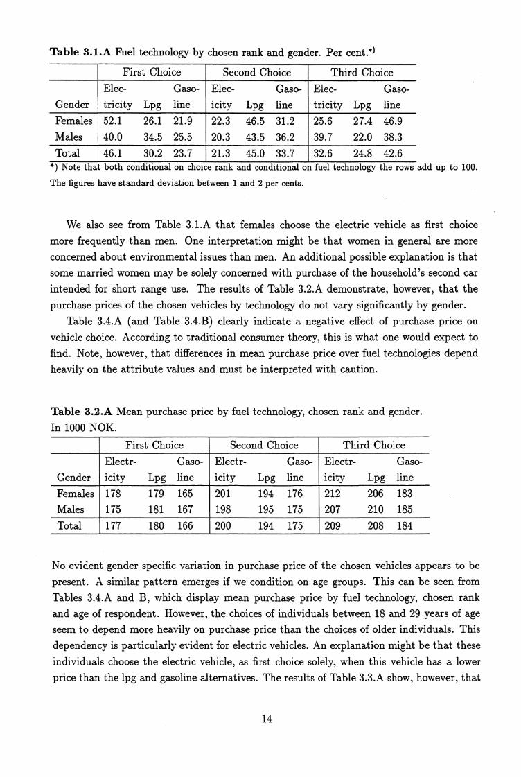
Table 3.1.A Fuel technology by chosen rank and gender. Per cent.*)

First Choice Second Choice Third Choice

Gender

Elec-tricity Lpg

Gaso-

line

Elec-

icity LpgGaso-line

Elec-

tricity LpgGaso-line

Females

Males

52.1

40.0

26.1

34.5

21.9

25.522.3

20.3

46.5

43.5

31.2

36.2

25.6

39.7

27.4

22.0

46.9

38.3

Total 46.1 30.2 23.7 21.3 45.0 33.7 32.6 24.8 42.6*) Note that both conditional on choice rank and conditional on fuel technology the rows add up to 100.

The figures have standard deviation between 1 and 2 per cents.

We also see from Table 3.1.A that females choose the electric vehicle as first choice

more frequently than men. One interpretation might be that women in general are more

concerned about environmental issues than men. An additional possible explanation is that

some married women may be solely concerned with purchase of the household's second car

intended for short range use. The results of Table 3.2.A demonstrate, however, that the

purchase prices of the chosen vehicles by technology do not vary significantly by gender.

Table 3.4.A (and Table 3.4.B) clearly indicate a negative effect of purchase price on

vehicle choice. According to traditional consumer theory, this is what one would expect to

find. Note, however, that differences in mean purchase price over fuel technologies depend

heavily on the attribute values and must be interpreted with caution.

Table 3.2.A Mean purchase price by fuel technology, chosen rank and gender.

In 1000 NOK.


Gender

Electr-icity Lpg

Gaso-line

Electr-

icity LpgGaso-line

Electr-icity Lpg

Gaso-line

Females

Males178175

179181

165167

201198

194195

176175

212207

206

210

183

185

Total 177 180 166 200 194 175 209 208 184

No evident gender specific variation in purchase price of the chosen vehicles appears to be

present. A similar pattern emerges if we condition on age groups. This can be seen from

Tables 3.4.A and B, which display mean purchase price by fuel technology, chosen rank

and age of respondent. However, the choices of individuals between 18 and 29 years of age

seem to depend more heavily on purchase price than the choices of older individuals. This

dependency is particularly evident for electric vehicles. An explanation might be that these

individuals choose the electric vehicle, as first choice solely, when this vehicle has a lower

price than the lpg and gasoline alternatives. The results of Table 3.3.A show, however , that

14

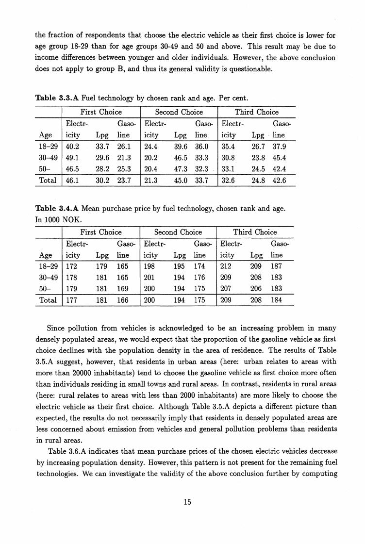
the fraction of respondents that choose the electric vehicle as their first choice is lower forage group 18-29 than for age groups 30-49 and 50 and above. This result may be due toincome differences between younger and older individuals. However, the above conclusiondoes not apply to group B, and thus its general validity is questionable.

Table 3.3.A Fuel technology by chosen rank and age. Per cent.


Electr- Gaso- Electr- Gaso- Electr- Gaso-

Age icity Lpg line icity Lpg line icity Lpg - line

18-29 40.2 33.7 26.1 24.4 39.6 36.0 ' 35.4 26.7 37.930-49 49.1 29.6 21.3 20.2 46.5 33.3 30.8 23.8 45.4

50- 46.5 28.2 25.3 20.4 47.3 32.3 • 33.1 24.5 42.4

Total 46.1 30.2 23.7 21.3 45.0 33.7 32.6 24.8 42.6

Table 3.4.A Mean purchase price by fuel technology, chosen rank and age.

In 1000 NOK.


Electr- Gaso- ' Electr- Gaso- Electr- Gaso-

Age icity Lpg line icity Lpg line icity Lpg line

18-29 172 179 165 198 195 174 212 209 187

30-49 178 181 165 201 194 176 209 208 183

50- 179 181 169 200 194 175 207 206 183

Total 177 181 166 200 194 175 209 208 184

Since pollution from vehicles is acknowledged to be an increasing problem in many

densely populated areas, we would expect that the proportion of the gasoline vehicle as first

choice declines with the population density in the area of residence. The results of Table

3.5.A suggest, however, that residents in urban areas (here: urban relates to areas withmore than 20000 inhabitants) tend to choose the gasoline vehicle as first choice more often

than individuals residing in small towns and rural areas. In contrast, residents in rural areas

(here: rural relates to areas with less than 2000 inhabitants) are more likely to choose the

electric vehicle as their first choice. Although Table 3.5.A depicts a different picture than

expected, the results do not necessarily imply that residents in densely populated areas are

less concerned about emission from vehicles and general pollution problems than residents

in rural areas.Table 3.6.A indicates that mean purchase prices of the chosen electric vehicles decrease

by increasing population density. However, this pattern is not present for the remaining fuel

technologies. We can investigate the validity of the above conclusion further by computing

15

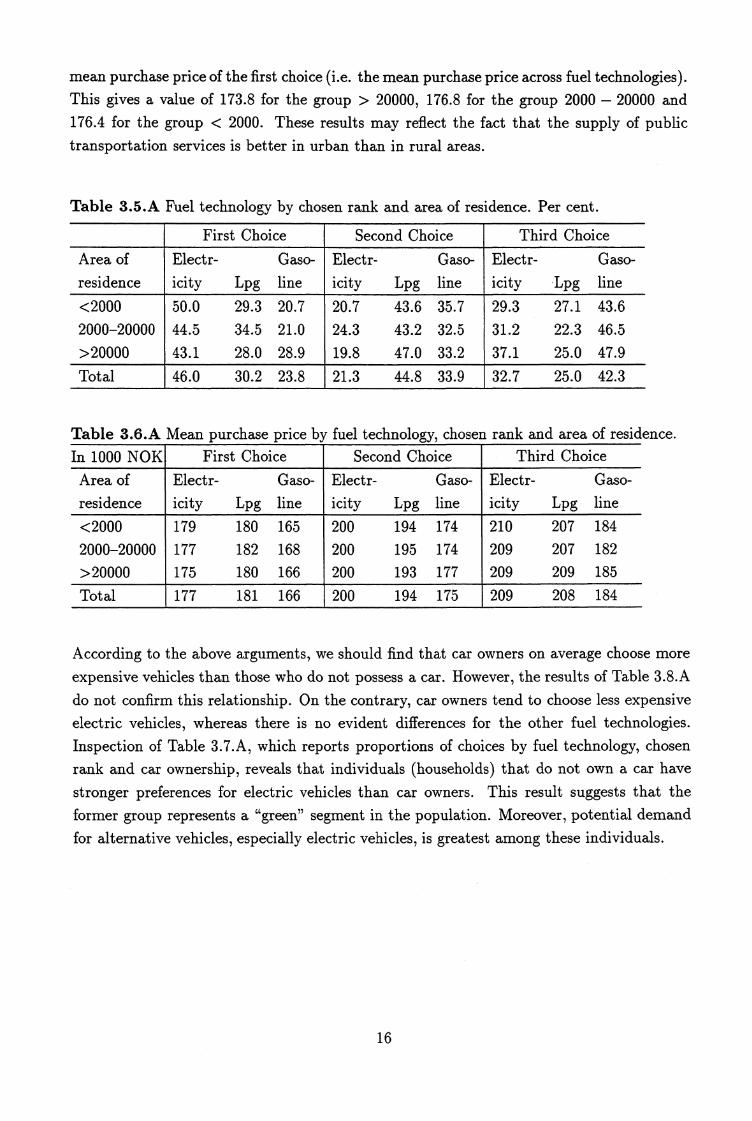
mean purchase price of the first choice (i.e. the mean purchase price across fuel technologies).This gives a value of 173.8 for the group > 20000, 176.8 for the group 2000 - 20000 and

176.4 for the group < 2000. These results may reflect the fact that the supply of public

transportation services is better in urban than in rural areas.

Table 3.5.A Fuel technology by chosen rank and area of residence. Per cent.


Area of Electr- Gaso- Electr- Gaso- Electr- Gaso-

residence icity Lpg line icity Lpg line icity Lpg line

<2000 50.0 29.3 20.7 20.7 43.6 35.7 29.3 27.1 43.62000-20000 44.5 34.5 21.0 24.3 43.2 32.5 31.2 22.3 46.5

>20000 43.1 28.0 28.9 19.8 47.0 33.2 37.1 25.0 47.9

Total 46.0 30.2 23.8 21.3 44.8 33.9 32.7 25.0 42.3

Table 3.6.A Mean purchase price by fuel technology, chosen rank and area of residence.

In 1000 NOK , First Choice Second Choice Third Choice

Area of Electr- Gaso- Electr- Gaso- Electr- Gaso-

residence icity Lpg line icity Lpg line icity Lpg line

<2000 179 180 165 200 194 174 210 207 184

2000-20000 177 182 168 200 195 174 209 207 182

>20000 175 180 166 200 193 177 209 209 185

Total 177 181 166 ' 200 194 175 209 208 184

According to the above arguments, we should find that car owners on average choose more

expensive vehicles than those who do not possess a car. However, the results of Table 3.8.A

do not confirm this relationship. On the contrary, car owners tend to choose less expensive

electric vehicles, whereas there is no evident differences for the other fuel technologies.

Inspection of Table 3.7.A, which reports proportions of choices by fuel technology, chosen

rank and car ownership, reveals that individuals (households) that do not own a car have

stronger preferences for electric vehicles than car owners. This result suggests that the

former group represents a "green" segment in the population. Moreover, potential demand

for alternative vehicles, especially electric vehicles, is greatest among these individuals.

16

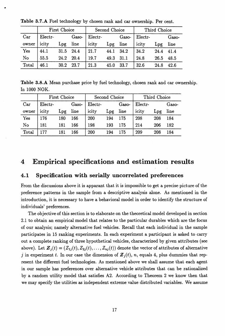
Table 3.7.A Fuel technology by chosen rank and car ownership. Per cent.

First Choice Second Choice Third ChoiceCar

owner

Electr-

icity Lpg

Gaso-

line

Electr-

icity Lpg

Gaso-

line

Electr-

icity LpgGaso-line

Yes

No44.1

55.531.524.2

24.4

20.4

21.7

19.7

44.1

49.3

34.2

31.134.2

24.824.4

26.5

41.4

48.5Total 46.1 30.2 23.7 21.3 45.0 33.7 32.6 24.8 42.6

Table 3.8.A Mean purchase price by fuel technology, chosen rank and car ownership.In 1000 NOK.


Carowner

Electr-icity Lpg

Gaso-line

Electr-

icity LpgGaso-line

Electr-

icity LpgGaso-line

Yes

No176

181180181

166

166

200

198

194

193

175175

208214

208

206

184

182

Total 177 181 166 200 194 175 209 208 184

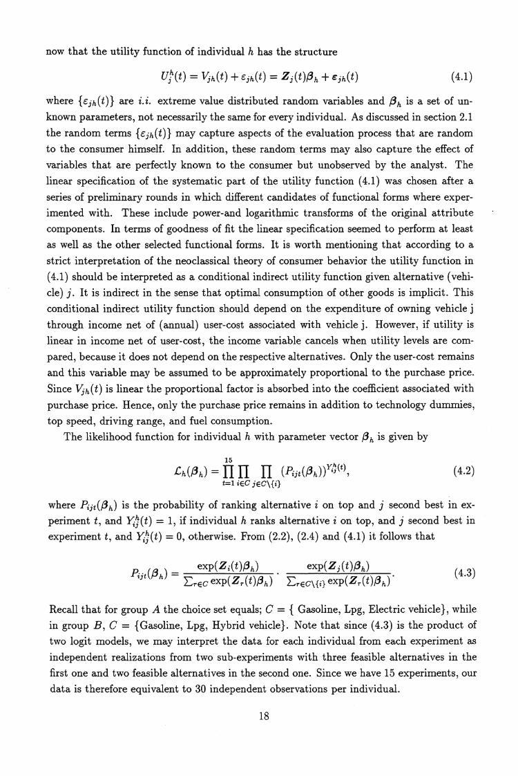
4 Empirical specifications and estimation results

4.1 Specification with serially uncorrelated preferences

From the discussions above it is apparant that it is impossible to get a precise picture of the

preference patterns in the sample from a descriptive analysis alone. As mentioned in the

introduction, it is necessary to have a behavioral model in order to identify the structure of

individuals' preferences.

The objective of this section is to elaborate on the theoretical model developed in section

2.1 to obtain an empirical model that relates to the particular durables which are the focus

of our analysis; namely alternative fuel vehicles. Recall that each individual in the sample

participates in 15 ranking experiments. In each experiment a participant is asked to carry

out a complete ranking of three hypothetical vehicles, characterized by given attributes (see

above). Let Z.; (t) = (Zii(t), Z2i(t), Zni(t)) denote the vector of attributes of alternative

j in experiment t. In our case the dimension of Zi (t), n, equals 4, plus dummies that rep-

resent the different fuel technologies. As mentioned above we shall assume that each agent

in our sample has preferences over alternative vehicle attributes that can be rationalized

by a random utility model that satisfies A2. According to Theorem 2 we know then that

we may specify the utilities as independent extreme value distributed variables. We assume

17

now that the utility function of individual h has the structure

UI(t) =Vih (t)+ ejh(t) = Zi (t)O h + eh(t) (4.1)

where { eih (t)} are i.i. extreme value distributed random variables and Oh is a set of un-

known parameters, not necessarily the same for every individual. As discussed in section 2.1the random terms {ejh(t)} may capture aspects of the evaluation process that are random

to the consumer himself. In addition, these random terms may also capture the effect of

variables that are perfectly known to the consumer but unobserved by the analyst. The

linear specification of the systematic part of the utility function (4.1) was chosen after a

series of preliminary rounds in which different candidates of functional forms where exper-

imented with. These include power-and logarithmic transforms of the original attribute

components. In terms of goodness of fit the linear specification seemed to perform at least

as well as the other selected functional forms. It is worth mentioning that according to a

strict interpretation of the neoclassical theory of consumer behavior the utility function in.

(4.1) should be interpreted as a conditional indirect utility function given alternative (vehi-

cle) j. It is indirect in the sense that optimal consumption of other goods is implicit. This

conditional indirect utility function should depend on the expenditure of owning vehicle j

through income net of (annual) user-cost associated with vehicle j. However, if utility is

linear in income net of user-cost, the income variable cancels when utility levels are corn-

pared, because it does not depend on the respective alternatives. Only the user-cost remains

and this variable may be assumed to be approximately proportional to the purchase price.

Since Vih (t) is linear the proportional factor is absorbed into the coefficient associated with

purchase price. Hence, only the purchase price remains in addition to technology dummies,

top speed, driving range, and fuel consumption.

The likelihood function for individual h with parameter vector 13 h is given by

15

Loh) = 11 (Pi3t(oh)) (t) , (4.2)

t=1 iEC jEC\fil

where Piji (O h) is the probability of ranking alternative i on top and j second best in ex-

periment t, and Y(t) = 1, if individual h ranks alternative i on top, and j second best in

experiment t, and Y(t) 0, otherwise. From (2.2), (2.4) and (4.1) it follows that

Piit(Oh)exp(Zi(t)Oh) exp(Zi(t)Oh) (4.3)

ErEcexp(zr(t)Oh) ErEcvilexp(zr(t )Oh)

Recall that for group A the choice set equals; C = { Gasoline, Lpg, Electric vehicle}, while

in group B, C = {Gasoline, Lpg, Hybrid vehicle). Note that since (4.3) is the product of

two logit models, we may interpret the data for each individual from each experiment as

independent realizations from two sub-experiments with three feasible alternatives in the

first one and two feasible alternatives in the second one. Since we have 15 experiments, our

data is therefore equivalent to 30 independent observations per individual.

18

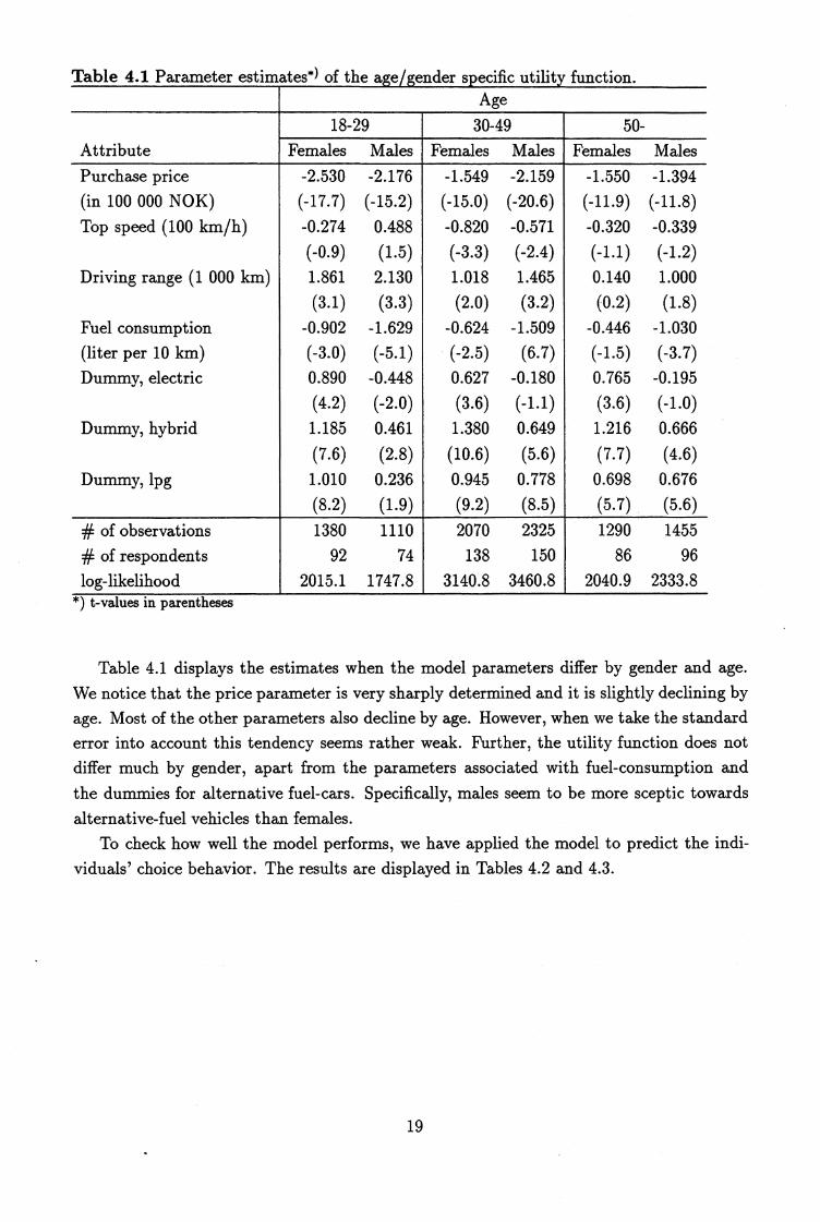
Table 4.1 Parameter estimates*) of the age/gender s ecific utility function.Age

18-29 30-49 50-Attribute Females Males Females Males Females Males

Purchase price -2.530 -2.176 -1.549 -2.159 -1.550 -1.394(in 100 000 NOK) (-17.7) (-15.2) (-15.0) (-20.6) (-11.9) (-11.8)Top speed (100 km/h) -0.274 0.488 -0.820 -0.571 -0.320 -0.339

(-0.9) (1.5) (-3.3) (-2.4) (-1.1) (-1.2)Driving range (1 000 km) 1.861 2.130 1.018 1.465 0.140 1.000

(3.1) (3.3) (2.0) (3.2) (0.2) (1.8)Fuel consumption -0.902 -1.629 -0.624 -1.509 -0.446 -1.030(liter per 10 km) (-3.0) (-5.1) (-2.5) (6.7) (-1.5) (-3.7)Dummy, electric 0.890 -0.448 0.627 -0.180 0.765 -0.195

(4.2) (-2.0) (3.6) (-1 .1) (3.6) (-1.0)Dummy, hybrid 1.185 0.461 1.380 0.649 1.216 0.666

(7.6) (2.8) (10.6) (5.6) (7.7) (4.6)Dummy, lpg 1.010 0.236 0.945 0.778 0.698 0.676

(8.2) (1.9) (9.2) (8.5) (5.7) (5.6)# of observations 1380 1110 2070 2325 1290 1455# of respondents 92 74 138 150 86 96log-likelihood 2015.1 1747.8 3140.8 3460.8 2040.9 2333.8

*) t-values in parentheses

Table 4.1 displays the estimates when the model parameters differ by gender and age.

We notice that the price parameter is very sharply determined and it is slightly declining by

age. Most of the other parameters also decline by age. However, when we take the standard

error into account this tendency seems rather weak. Further, the utility function does not

differ much by gender, apart from the parameters associated with fuel-consumption and

the dummies for alternative fuel-cars. Specifically, males seem to be more sceptic towards

alternative-fuel vehicles than females.

To check how well the model performs, we have applied the model to predict the indi-

viduals' choice behavior. The results are displayed in Tables 4.2 and 4.3.

19

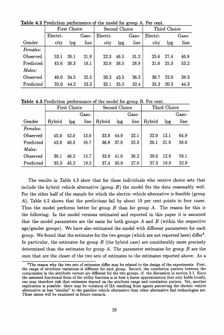
Table 4.2 Prediction Derformence of the model for rou A. Per cent.First Choice Second Choice Third Choice

Electri- Gaso- Electri- Gaso- Electri- Gaso-

Gender city lpg line city lpg line city lpg line

Females:

Observed 52.1 26.1 21.9 22.3 46.5 31.2 25.6 27.4 46.9Predicted 45.6 36.3 18.1 32.8 38.5 28.8 21.6 25.3 53.2

Males:

Observed 40.0 34.5 25.5 20.3 43.5 36.2 39.7 22.0 38.3

Predicted 32.6 44.2 23.3 32.1 35.5 32.4 35.3 20.3 44.3

Table 4.3 Prediction performance of the model for group B. Per cent.First Choice Second Choice Third Choice

Gaso- Gaso- Gaso-

Gender Hybrid ipg line Hybrid lpg line Hybrid lpg line

Females:

Observed 45.0 42.0 13.0 33.0 44.9 22.1 22.0 13.1 64.9

Predicted 43.0 40.3 16.7 36.9 37.8 25.3 20.1 21.9 58.0

Males:

Observed 38.1 46.2 15.7 32.9 41.0 26.2 29.0 12.8 58.1

Predicted 35.3 45.2 19.5 37.4 35.0 27.6 27.3 19.8 52.9

The results in Table 4.3 show that for those individuals who receive choice sets that

include the hybrid vehicle alternative (group B) the model fits the data reasonably well.

For the other half of the sample for which the electric vehicle alternative is feasible (group

A), Table 4.2 shows that the predictions fail by about 10 per cent points in four cases.

Thus the model performs better for group B than for group A. The reason for this is

the following: In the model versions estimated and reported in this paper it is assumed

that the model parameters are the same for both groups A and B (within the respective

age/gender groups). We have also estimated the model with different parameters for each

group. We found that the estimates for the two groups (which are not reported here) differ4 .

In particular, the estimates for group B (the hybrid case) are considerably more precisely

determined than the estimates for group A. The parameter estimates for group B are the

ones that are the closer of the two sets of estimates to the estimates reported above. As a

'The reason why the two sets of estimates differ may be related to the design of the experiments. First,the range of attribute variations is different for each group. Second, the correlation pattern between thecomponents in the attribute vectors are different for the two groups, cf. the discussion in section 3.1. Sincethe assumed functional form of the utility function is at best a linear approximation that only holds locally,one may therefore risk that estimates depend on the attribute range and correlation pattern. Yet, anotherexplication is possible: there may be violation of IIA resulting from agents perceiving the electric vehiclealternative as less "similar" to the gasoline vehicle alternative than other alternative fuel technologies are.These issues will be examined in future research.

20

result, the predictions from the model tend to be better for group B than for group A.

4.2 Random coefficient specification

In general, the parameters may vary across individuals. In some cases this variation maybe accounted for by introducing individual characteristics such as age, education, etc. It is,however, a common experience that the available observable characteristics are insufficientfor removing all the heterogeneity in the systematic terms of the utility function. Note

that, in our case, since we have data equivalent to 30 observations for each individual, itis, at least in principle, possible to estimate individual specific parameters. Thus, as an

alternative approach we employ a random coefficient specification in which the parametervectors of the individuals are viewed as independent draws from a multivariate probability

distribution F, say. Consequently, the likelihood function will in this case take the form

ELh( 13) f rh(f3)dF( 13) (4.4)

and the total log likelihood function becomes

in = Eln(E4(0)). (4.5)h

The maximum likelihood procedure is now to estimate the parameters of F, or in case a

semi-parametric approach is taken, a non-parametric estimate of F.In the estimation of the model we consider three cases. In the first case the parameters are

assumed to be distributed across individuals according to a multivariate normal distribution

with components that are independent apart from the parameters related to the technology

dummies. In the second case the parameters are assumed to be distributed according to a

nonparametric distribution. Finally, we have also estimated individual specific parameters

but these estimates turned out to be rather imprecise and are therefore not reported here. In

the nonparametric case F(0) is assumed to be a multinomial distribution with probability

mass at points f3 1, 2, ..., d, (say). Estimation of multinomial logit models with random

coefficients distributed according to a multinomial distribution has been considered by Jain

et al. (1994). In practice this may be a rather tricky task because the corresponding

likelihood function often may have several local maxima and it may be difficult to locate

every one of them. In the present case this turned out to be so, in fact we have found

numerous local maxima. We therefore cannot guarantee that the estimation results we

have found so far correspond to the global maximum of the likelihood. We have therefore

abandoned the case with a nonparametric distribution of the parameters in this paper, but

we will pursue the issue in the future.

A drawback with the normallity assumption is that when large coefficient heterogeneityis present a considerable proportion of the sample may get the wrong sign of the price

coefficients since the normal distribution is symmetric about the mean. From Table 4.7

in Appendix III we realize that this is indeed what turns out to be the case here and we

21

therefore conclude that this strategy is inappropriate. Other alternatives will be consideredin future research.

4.3 Allowing for serially correlated preferences

In this section we shall consider the empirical specification and estimation of the model

version discussed in subsection 2.2, where the utility functions are correlated across experi-

ments.

Let W(t) be equal to one if individual h ranks alternative i on top in experiment t — 1

and j on top in experiment t. Then the likelihood function for the first choices of individual

h can be written as

15

Loh,oh.) = H -t=2 iEC jEC

1, owth.,(t) H p3h(1)wi;(1)3Ec

(4.6)

where TV(1) is equal to one if individual h ranks alternative j on top in the first experiment

and zero otherwise.

Recall that the likelihood function (4.6) corresponds to the observations on individu-

als' first choices. As mentioned in section 2.2, the structure of the corresponding choice

probabilities for complete rank orderings are not known and we are therefore unable to

utilize the full set of observations when estimating the model. However, the remaining

set of observations on individuals' second choices can be applied to test the model since

these observations enable us to perform out-of-sample predictions. It is a well acknowledged

principle that out-of-sample observations are necessary to put a model to serious test. In

particular, it enables us to check the IIA assumption which is a crucial assumption in all

the model versions discussed in this paper.

22

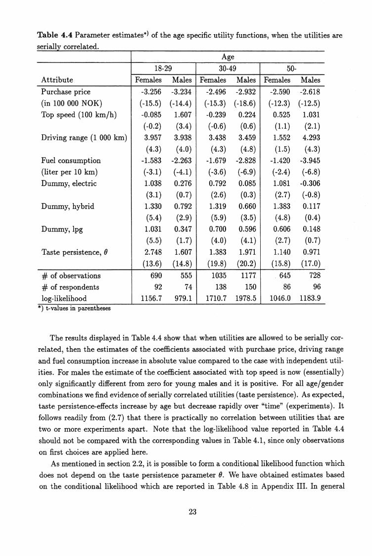
Table 4.4 Parameter estimates*) of the age specific utility functions, when the utilities are

serially correlated.Age


Purchase price -3.256 -3.234 -2.496 -2.932 -2.590 -2.618(in 100 000 NOK) (-15.5) (-14.4) (-15.3) (-18.6) (-12.3) (-12.5)Top speed (100 km/h) -0.085 1.607 -0.239 0.224 0.525 1.031

(-0.2) (3.4) (-0.6) (0.6) (1.1) (2.1)

Driving range (1 000 km) 3.957 3.938 3.438 3.459 1.552 4.293(4.3) (4.0) (4.3) (4.8) (1.5) (4.3)

Fuel consumption -1.583 -2.263 -1.679 -2.828 -1.420 -3.945(liter per 10 km) (-3.1) (-4.1) (-3.6) (-6.9) (-2.4) (-6.8)

Dummy, electric 1.038 0.276 0.792 0.085 1.081 -0.306

(3.1) (0.7) (2.6) (0.3) (2.7) (-0.8)

Dummy, hybrid 1.330 0.792 1.319 0.660 1.383 0.117

(5.4) (2.9) (5.9) (3.5) (4.8) (0.4)

Dummy, lpg 1.031 0.347 0.700 0.596 0.606 0.148

(5.5) (1.7) (4.0) (4.1) (2.7) (0.7)

Taste persistence, 0 2.748 1.607 1.383 1.971 1.140 0.971

(13.6) (14.8) (19.8) (20.2) (15.8) (17.0)

# of observations 690 555 1035 1177 645 728

# of respondents 92 74 138 150 86 96

log-likelihood 1156.7 979.1 1710.7 1978.5 1046.0 1183.9*) t-values in parentheses

The results displayed in Table 4.4 show that when utilities are allowed to be serially cor-

related, then the estimates of the coefficients associated with purchase price, driving range

and fuel consumption increase in absolute value compared to the case with independent util-

ities. For males the estimate of the coefficient associated with top speed is now (essentially)

only significantly different from zero for young males and it is positive. For all age/gender

combinations we find evidence of serially correlated utilities (taste persistence). As expected,

taste persistence-effects increase by age but decrease rapidly over "time" (experiments). It

follows readily from (2.7) that there is practically no correlation between utilities that are

two or more experiments apart. Note that the log-likelihood value reported in Table 4.4

should not be compared with the corresponding values in Table 4.1, since only observations

on first choices are applied here.

As mentioned in section 2.2, it is possible to form a conditional likelihood function which

does not depend on the taste persistence parameter O. We have obtained estimates based

on the conditional likelihood which are reported in Table 4.8 in Appendix III. In general

23

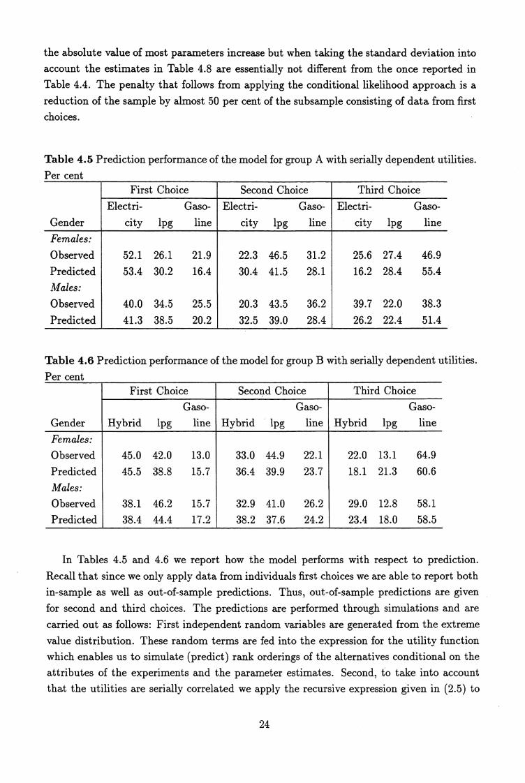
the absolute value of most parameters increase but when taking the standard deviation intoaccount the estimates in Table 4.8 are essentially not different from the once reported inTable 4.4. The penalty that follows from applying the conditional likelihood approach is areduction of the sample by almost 50 per cent of the subsample consisting of data from firstchoices.

Table 4.5 Prediction performance of the model for group A with serially dependent utilities.Per cent


Electri- Gaso- Electri- Gaso- Electri- Gaso-

Gender city ipg line city lpg line city lpg line

Females:

Observed 52.1 26.1 21.9 22.3 46.5 31.2 25.6 27.4 46.9

Predicted 53.4 30.2 16.4 30.4 41.5 28.1 16.2 28.4 55.4

Males:

Observed 40.0 34.5 25.5 20.3 43.5 36.2 39.7 22.0 38.3

Predicted 41.3 38.5 20.2 32.5 39.0 28.4 26.2 22.4 51.4

Table 4.6 Prediction performance of the model for group B with serially dependent utilities.

Per centFirst Choice Second Choice Third Choice

Gaso- Gaso- Gaso-

Gender Hybrid lpg line Hybrid • lpg line Hybrid lpg line

Females:

Observed 45.0 42.0 13.0 33.0 44.9 22.1 22.0 13.1 64.9

Predicted 45.5 38.8 15.7 36.4 39.9 23.7 18.1 21.3 60.6

Males:

Observed 38.1 46.2 15.7 32.9 41.0 26.2 29.0 12.8 58.1

Predicted 38.4 44.4 17.2 38.2 37.6 24.2 23.4 18.0 58.5

In Tables 4.5 and 4.6 we report how the model performs with respect to prediction.

Recall that since we only apply data from individuals first choices we are able to report both

in-sample as well as out-of-sample predictions. Thus, out-of-sample predictions are given

for second and third choices. The predictions are performed through simulations and are

carried out as follows: First independent random variables are generated from the extreme

value distribution. These random terms are fed into the expression for the utility functionwhich enables us to simulate (predict) rank orderings of the alternatives conditional on the

attributes of the experiments and the parameter estimates. Second, to take into accountthat the utilities are serially correlated we apply the recursive expression given in (2.5) to

24

update the utilities to the next period (experiment). The simulations are replicated a largenumber of times to eliminate simulation error.

The tables demonstrate that predictions are improved as regards to first choices (whichare within-sample predictions), but that predictions for second and third choices (which areout-of-sample predictions) are not improved compared to the case with serially uncorrelatedutilities.

Elasticities and the willingness to pay for alter-

native fuel vehicles

By means of the estimated model it is possible to compute elasticities and compensation

variation measures. In our context compensating variation (CV) means the amount that

must be added to the purchase price of a specific vehicle technology to obtain the same

utility, ceteris paribus, as the reference technology. A standard approach is to compute CV

by applying the mean of the utility function only, (cf. Small and Rosen, (1981)). This ignores

the heterogeneity in the model. Since we have formulated and estimated a random utility

model it is possible to take the random taste-shifters into account when computing CV.

In this way CV also becomes random and one must derive the corresponding distribution

function. In our case this turns out to be simple due to the fact that the mean utility function

is linear and the random terms are extreme value distributed. If the random terms of CV

are interpreted as random to the agent himself the distribution function of CV describes

the likelihood of the different levels of CV. If however, the randomness is solely attributed

to unobserved population heterogeneity this distribution function describes how CV vary

across the population due to unobservables that are perfectly known to the agents.

Consider first the elasticities. For the purpose of computing elasticities of the choice

probabilities note that by (2.12)

P. = exp(Zif3)

.1 Er exp(Z,O) •

By straight forward calculus we obtain the following expressions,

a log P.;

— Z1 — P.a log Zis

and

a log Pi = —Zks AsPi • (5.3)a log Zks

for k j. Equation (5.2) expresses the own-attribute elasticity of Pj with respect to compo-

nent Zjs while (5.3) expresses the corresponding formulae for the cross-attribute elasticity.

(5. 1)

(5.2)

25

Age

Technology

Electricity

Hybrid

Lpg

Gasoline

18-29

Females Males

0.27

0.22

0.36

0.37

0.27

0.24

0.10

0.17

30-49Females Males

0.25

0.19

0.42

0.33

0.22

0.31

0.11

0.17

50-

Females Males

0.30 0.18

0.41 0.28

0.19 0.29

0.10 0.25

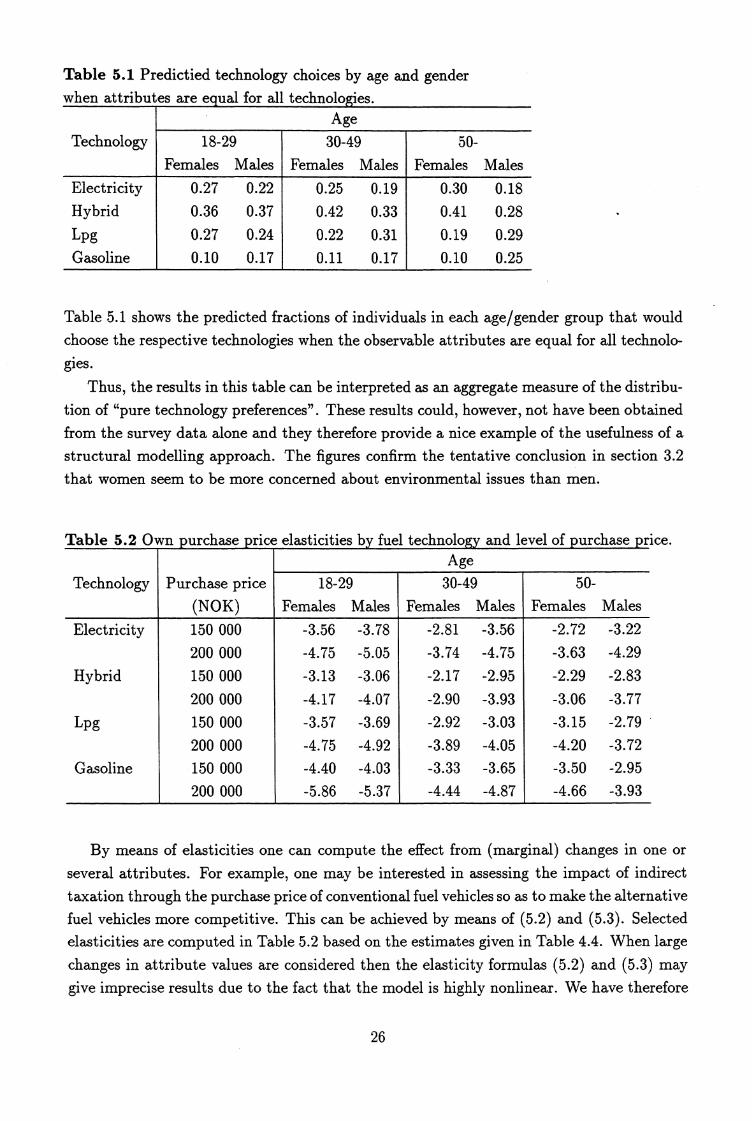
Table 5.1 Predictied technology choices by age and genderwhen attributes are equal for all technologies.

Table 5.1 shows the predicted fractions of individuals in each age/gender group that would

choose the respective technologies when the observable attributes are equal for all technolo-

gies.

Thus, the results in this table can be interpreted as an aggregate measure of the distribu-

tion of "pure technology preferences". These results could, however, not have been obtained

from the survey data alone and they therefore provide a nice example of the usefulness of a

structural modelling approach. The figures confirm the tentative conclusion in section 3.2

that women seem to be more concerned about environmental issues than men.

Table 5.2 Own purchase price elasticities by fuel technology and level of purchase price.Age

Purchase price

(NOK)

150 000

200 000

150 000

200 000150 000

200 000150 000

200 000

18-29Females Males

-3.56 -3.78

-4.75 -5.05

-3.13 -3.06

-4.17 -4.07-3.57 -3.69-4.75 -4.92-4.40 -4.03

-5.86 -5.37

30-49Females Males

-2.81 -3.56-3.74 -4.75

-2.17 -2.95

-2.90 -3.93-2.92 -3.03-3.89 -4.05-3.33 -3.65-4.44 -4.87

50-Females Males

-2.72 -3.22

-3.63 -4.29

-2.29 -2.83

-3.06 -3.77

-3.15 -2.79

-4.20 -3.72

-3.50 -2.95

-4.66 -3.93

Technology

Electricity

Hybrid

Lpg

Gasoline

By means of elasticities one can compute the effect from (marginal) changes in one or

several attributes. For example, one may be interested in assessing the impact of indirect

taxation through the purchase price of conventional fuel vehicles so as to make the alternative

fuel vehicles more competitive. This can be achieved by means of (5.2) and (5.3). Selected

elasticities are computed in Table 5.2 based on the estimates given in Table 4.4. When large

changes in attribute values are considered then the elasticity formulas (5.2) and (5.3) may

give imprecise results due to the fact that the model is highly nonlinear. We have therefore

26

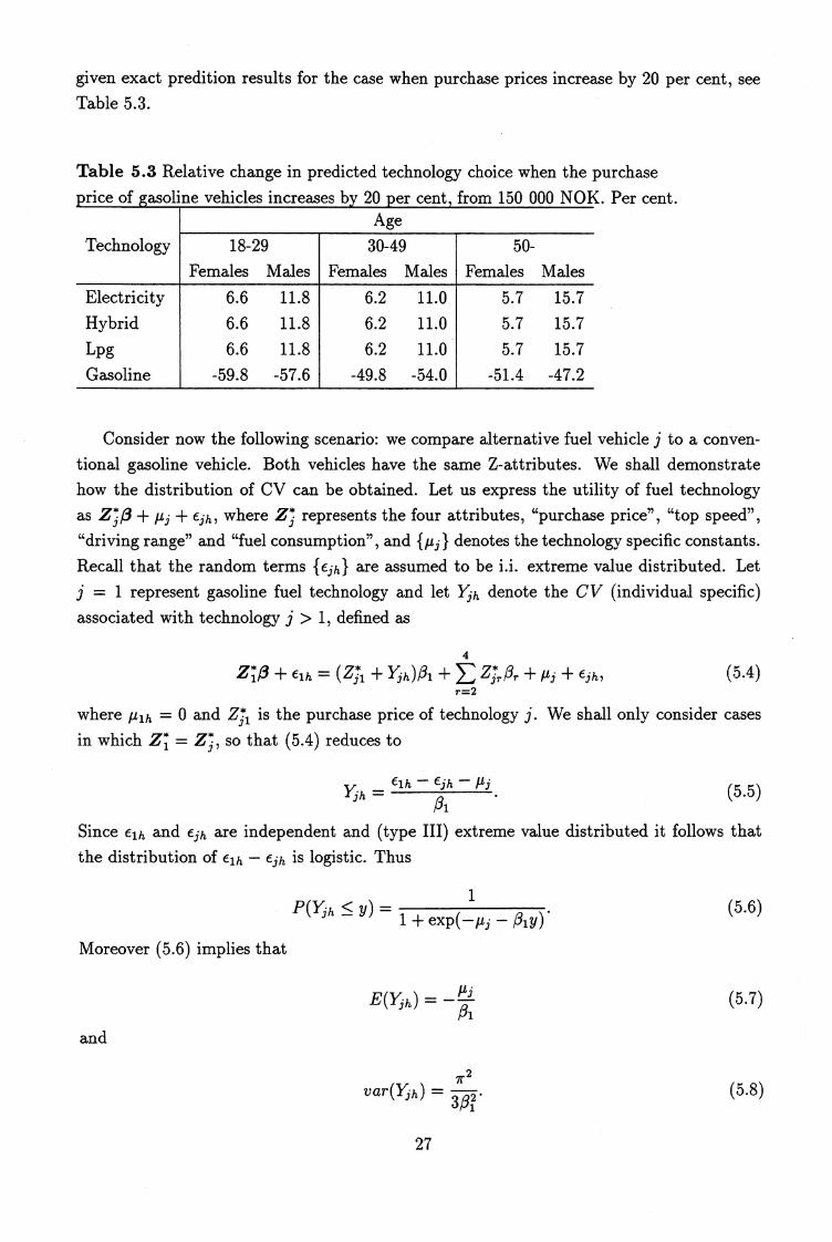
given exact predition results for the case when purchase prices increase by 20 per cent, seeTable 5.3.

Table 5.3 Relative change in predicted technology choice when the purchaseprice of gasoline vehicles increases by 20 per cent, from 150 000 NOK. Per cent.

Age

Technology

Electricity

Hybrid

Lpg

Gasoline

18-29

Females Males

6.6

11.8

6.6

11.8

6.6

11.8

-59.8 -57.6

30-49Females Males

6.2 11.0

6.2 11.0

6.2 11.0

-49.8 -54.0

50-Females Males

5.7 15.7

5.7 15.7

5.7 15.7

-51.4 -47.2

Consider now the following scenario: we compare alternative fuel vehicle j to a conven-

tional gasoline vehicle. Both vehicles have the same Z-attributes. We shall demonstratehow the distribution of CV can be obtained. Let us express the utility of fuel technology

as Eifi tti fjh, where Zy represents the four attributes, "purchase price", "top speed","driving range" and "fuel consumption", and {iz i } denotes the technology specific constants.

Recall that the random terms {ejh } are assumed to be i.i. extreme value distributed. Let

= 1 represent gasoline fuel technology and let Yjh denote the CV (individual specific)

associated with technology j > 1, defined as

4

Z1/3 + 61h = (Z71 + Yih)ß1 +E z7ror + j (5.4)

r=2

where A ih = 0 and Z71 is the purchase price of technology j. We shall only consider cases

in which Z1 = Z;, so that (5.4) reduces to

Yjh = 61h - Ejh - Pi

01

(5.5)

Since elh and ejh are independent and (type III) extreme value distributed it follows that

the distribution of elh ejh is logistic. Thus

1 P(Yjh Y) = 1+ exP(-Pj AN) *

Moreover (5.6) implies that

E( Yjh ) = -

and

71.2var(Y3h) = 2 .

3 /31

(5.6)

(5.7)

(5.8)

27

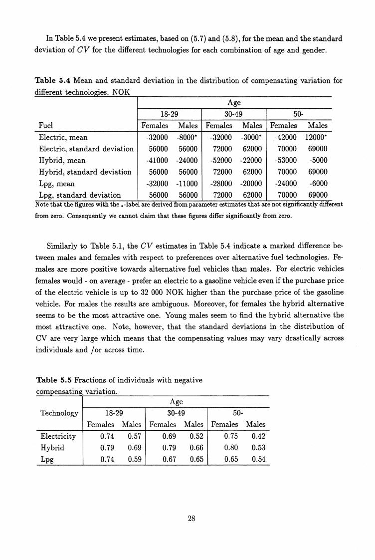
In Table 5.4 we present estimates, based on (5.7) and (5.8), for the mean and the standarddeviation of CV for the different technologies for each combination of age and gender.

Table 5.4 Mean and standard deviation in the distribution of compensating variation for

different technologies. NOKAge

18-29Females Males

-32000 -8000*

56000 56000

-41000 -24000

56000 56000

-32000 -1100056000 56000

30-49Females Males

-32000 -3000*

72000 62000

-52000 -2200072000 62000

-28000 -2000072000 62000

50-Females Males

-42000 12000*

70000 69000

-53000 -5000

70000 69000

-24000 -6000

70000 69000

Fuel

Electric, mean

Electric, standard deviation

Hybrid, mean

Hybrid, standard deviation

Lpg, mean

Lpg, standard deviationNote that the figures with the .-label are derived from parameter estimates that are not significantly different

from zero. Consequently we cannot claim that these figures differ significantly from zero.

Similarly to Table 5.1, the CV estimates in Table 5.4 indicate a marked difference be-

tween males and females with respect to preferences over alternative fuel technologies. Fe-

males are more positive towards alternative fuel vehicles than males. For electric vehicles

females would - on average - prefer an electric to a gasoline vehicle even if the purchase price

of the electric vehicle is up to 32 000 NOK higher than the purchase price of the gasoline

vehicle. For males the results are ambiguous. Moreover, for females the hybrid alternative

seems to be the most attractive one. Young males seem to find the hybrid alternative the

most attractive one. Note, however, that the standard deviations in the distribution of

CV are very large which means that the compensating values may vary drastically across

individuals and /or across time.

Table 5.5 Fractions of individuals with negative

compensating variation.Age

Technology

Electricity

Hybrid

Lpg

18-29Females Males

0.74 0.57

0.79 0.69

0.74 0.59

30-49Females Males

0.69 0.52

0.79 0.66

0.67 0.65

50-Females Males

0.75 0.42

0.80 0.53

0.65 0.54

28

In Table 5.5 we report the fraction of individuals with negative CV, as predicted by themodel. That is, these figures express the fractions of individuals which would prefer therespective alternative technologies to a gasoline vehicle when the (observable) attributes are

equal for all technologies. These figures are obtained by means of (5.6) with y O.

6 Conclusion

In this paper we have analyzed the demand for alternative fuel vehicles. The empiricalresults are based on a "stated preference" type of survey conducted on a sample of Norwegian

individuals. Different random utility models are formulated and estimated. They include

models with serially uncorrelated as well as serially correlated utility functions.

The empirical results show that alternative fuel vehicles appear to be fully competitive

alternatives compared to conventional gasoline vehicles. As regards electric vehicles, it seems

that (on average) men are more reserved towards this technology than women. This may

reflect the fact that so far there is considerable uncertainty about the battery technology

and men, more than women, may have doubts about whether or not it will be possible to

provide a sufficiently convenient infrastructure for servicing and refueling for electric vehicles

in the near future. Furthermore, the hybrid alternative appears to be the most preferred

technology among females and young males while males above 30 years of age seem more

or less indifferent between the hybrid and the lpg alternative.

29

References

Beggs, S., S. Cardell and J. Hausman (1981): Assessing the Potential Demand for ElectricCars, Journal of Econometrics 16, 1-19.

Block, H., and J. Marschak (1960): "Random Orderings and Stochastic Theories of Re-sponse" in Olkin et al. (eds.): Contributions to Probability and Statistics, Stanford:

Stanford University Press.

Bunch, D.S., M. Bradley, T.F. Golob, R. Kitamura and G.P. Occhiuzzo (1991): Demandfor Clean-fuel Personal Vehicles in California: A Discrete-Choice Stated PreferenceSurvey. Mimeo, University of California, Davis and Irvine.

Calfee, J.E. (1985): Estimating the Demand for Electric Automobiles using Fully Disag-gregated Probabilistic Choice Analysis, Transportation Research 19B, 287-302.

Dagsvik, J.K. (1983): Discrete and Dynamic Choice: An Extension of the Choice Models

of Luce and Thurstone, Journal of Mathematical Psychology 27, 1-43.

Dagsvik, J.K. (1988): Markov Chains Generated by Maximizing Components of Multidi-

mensional Extremal Processes, Stochastic Processes and their Applications 28, 31-45.

Dagsvik, J.K. (1995a): Dynamic Choice, Multistate Duration Models and Stochastic Struc-

ture, forthcoming in the series Discussion Papers, Statistics Norway.

Dagsvik, J.K. (1995b): The Structure of hitertemporal Models for Myopic Choice with

Random Preferences, Memorandum, 11/95, Department of Economics, University of

Oslo.

Debreu, G. (1960): Review of R.D. Luce, Individual Choice Behavior, American Economic

Review 50, 186-188.

Golob, T.F., R. Kitamura and G. Occhiuzzo (1991): The Effects of Consumer Beliefsand Environmental Concerns on the Market Potential for Alternative Fuel Vehicles.

Mimeo, University of California, Davis and Irvine.

Hensher, D.A. (1982): Functional Measurement, Individual Preferences and Discrete-

Choice Modeling: Theory and Application, Journal of Economic Psychology 2, 323-

335.

Jain, D.C., N. J. Vilcassim and P. K. Chintagunta (1994): A Random-Coefficient Logit

Brand-choice Model Applied to Panel Data, Journal of Business and Economic Statis-

tics 12, 317-328.

Levin, I.P., J.J. Louviere, A.A. Schepanski and K.L. Norman (1983): External Validity

Tests of Laboratory Studies of Information Integration, Organizational Behavior and

Human Performance 31, 173-193.

30

Louviere, J.J. (1988): Conjoint Analysis Modelling of Stated Preferences, Journal of Trans-port Economics and Policy 22, 93-119.

Luce, R.D. (1959): Individual Choice Behavior, New York:Wiley.

Luce, R.D., (1977): The Choice Axiom after Twenty Years, Journal of Mathematical Psy-chology 15, 215-233.

Luce, R.D. and P. Suppes (1965): "Preference, Utility and Subjective Probability" in R.D.Luce, R.R. Bush and E. Galanter (eds.): Handbook of Mathematical Psychology, Vol.III, New York: Wiley.

Mannering, F.L. and K. Train (1985): Recent Directions in Automobile Demand Modeling,Transportation Research 19B, 265-274.

McFadden, D. (1981): "Econometric Models of Probabilistic Choice" in D. McFadden andC.F. Manski (eds.): Structural Analysis of Discrete Data with Econometric Applica-

tions, Cambridge, Massachusetts: MIT Press.

Pearmain, D., J. Swanson, E. Kroes and M. Bradley (1991): Stated Preference Techniques:

A Guide to Practice, Richmond/Haag: Steer Davis Gleave/Hague Consulting Group.

Resnick, S., and R. Roy (1990): Multivariate Extremal Processes, Leader Processes andDynamic Choice Models, Advances in Applied Probability 22, 309-331.

Small, K.A., and H.S. Rosen (1981): Applied Welfare Economics with Discrete Choice

Models, Econometrica 49, 105-130.

Strauss, D. (1979): Some Results on Random Utility Models, Journal of Mathematical

Psychology 19, 35-51.

Strauss, D. and C.A. Robertson (1981): A Characterization Theorem for Random UtilityVariables, Journal of Mathematical Psychology 23, 273-286.

Suppes, P., D.H. Krantz, R.D. Luce and A. Tversky (1989): Foundations of Measurements,

Vol II. ch. 17, New York: Academic Press.

Thurstone, L.L. (1927): A Law of Comparative Judgment, Psychological Review 34, 272—

286.

Train, K. (1980): The Potential Market for Non-gasoline-powered Vehicles, Transportation

Research 14A, 405-414.

Tversky, A. (1969): Intransivity of Preferences, Psychological Review 76, 31-48.

Yellott (1977): The Relationship between Luce's Choice Axiom, Thurnstone's Theory

of Comparative Judgement, and the Double Exponential Distribution, Mathematical

Psychology 5, 109-144.

31

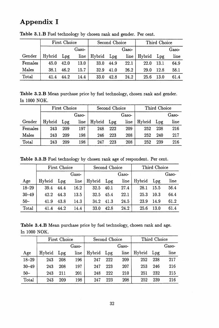
Appendix I

Table 3.1.B Fuel technology by chosen rank and gender. Per cent.

Gender


Gaso-

Hybrid Lpg lineGaso-

Hybrid Lpg line

Gaso-

Hybrid Lpg line

Females

Males45.0

38.1

42.0

46.2

13.0

15.733.0

32.9

44.9

41.0

22.1

26.2

22.0

29.013.112.8

64.958.1

Total 41.4 44.2 14.4 33.0 42.8 24.2 25.6 13.0 61.4

Table 3.2.B Mean purchase price by fuel technology, chosen rank and gender.

In 1000 NOK.

Gender


Gaso-Hybrid Lpg line

Gaso-

Hybrid Lpg line

Gaso-

Hybrid Lpg line

FemalesMales

243243

209209

197198

248246

222223

209208

252252

238240

216217

Total 243 209 198 247 223 208 252 239 216

Table 3.3.B Fuel technology by chosen rank age of respondent. Per cent.


Gaso- Gaso- Gaso-Age Hybrid Lpg line Hybrid Lpg line Hybrid Lpg line

18-29 39.4 44.4 16.2 32.5 40.1 27.4 28.1 15.5 56.4

30-49 42.2 44.3 13.5 32.5 45.4 22.1 25.3 10.3 64.4

50- 41.9 43.8 14.3 34.2 41.3 24.5 23.9 14.9 61.2

Total 41.4 44.2 14.4 ' 33.0 42.8 24.2 25.6 13.0 61.4

Table 3.4.B Mean purchase price by fuel technology, chosen rank and age.

In 1000 NOK.


Gaso- Gaso- Gaso-

Age Hybrid Lpg line Hybrid Lpg line Hybrid Lpg line

18-29 243 208 196 247 222 209 252 238 217

30-49 243 208 197 247 223 207 253 246 216

50- 243 211 201 248 222 210 251 232 215

Total 243 209 198 247 223 208 252 239 216

32

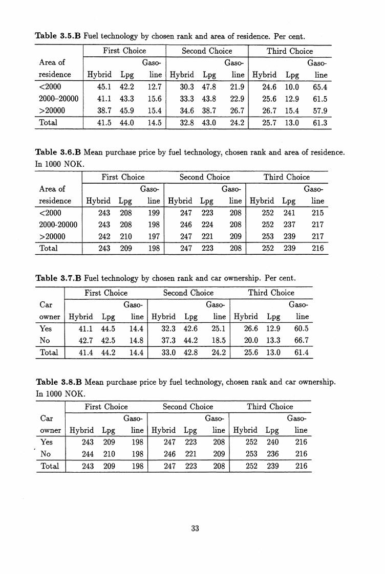
Area ofresidence

<20002000-20000

>20000Total

Gaso-

Hybrid Lpg line

243 208

199

243 208

198

242 210

197

243 209 198

Gaso-

Hybrid Lpg line

247 223

208

246 224

208

247 221

209

247 223 208

Third Choice

Gaso-

Hybrid Lpg line

252 241 215

252 237 217

253 239 217 252 239 216

First Choice Second Choice


Car

owner

Yes

No

Total

Gaso-

Hybrid Lpg line

41.1 44.5 14.4

42.7 42.5 14.8

41.4 44.2 14.4

Hybrid Lpg

Gaso-

line

Gaso-

Hybrid Lpg

line

26.6 12.9

60.5

20.0 13.3

66.7

25.6 13.0 61.4

32.3 42.6

25.1

37.3 44.2

18.5

33.0 42.8

24.2

Table 3.5.B Fuel technology by chosen rank and area of residence. Per cent.

Area of

residence

First Choice Second Choice Third ChoiceGaso-

Hybrid Lpg line

Gaso-

Hybrid Lpg lineGaso-

Hybrid Lpg line

<2000

2000-20000

>20000

45.1 42.2 12.7

41.1 43.3 15.6

38.7 45.9 15.4

30.3 47.8 21.9

33.3 43.8 22.9

34.6 38.7 26.7

24.6 10.0 65.4

25.6 12.9 61.5

26.7 15.4 57.9Total 41.5 44.0 14.5 32.8 43.0 24.2 25.7 13.0 61.3

Table 3.6.B Mean purchase price by fuel technology, chosen rank and area of residence.

In 1000 NOK.

Table 3.7.B Fuel technology by chosen rank and car ownership. Per cent.

Table 3.8.B Mean purchase price by fuel technology, chosen rank and car ownership.

In 1000 NOK.

First Choice

Second ChoiceGaso-

Hybrid Lpg line

Carowner

Yes

No

Total

243 209

198

244 210

198

Gaso-

Hybrid Lpg line

247 223

208

Third ChoiceGaso-

Hybrid Lpg line

252 240 216

253 236 216

252 239 216

208

209

247 223

246 221

243 209 198

33

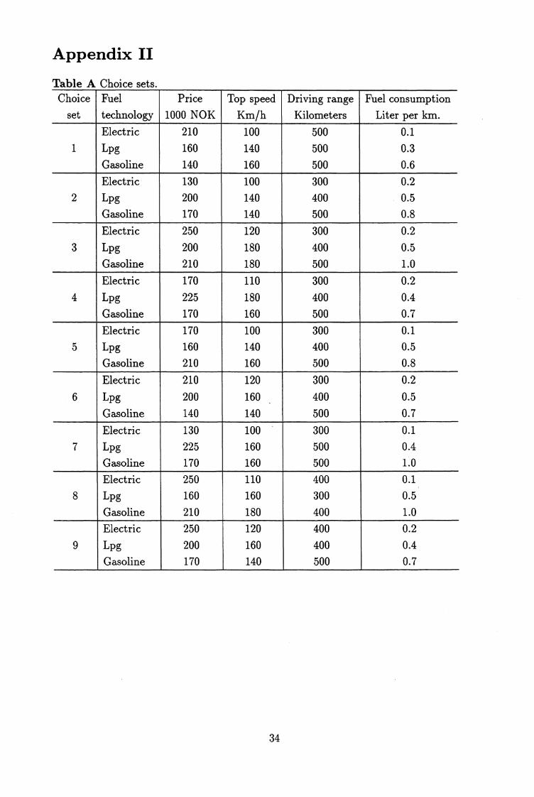
Appendix II

Table A Choice sets.Choice

set

Fuel

technology

Price

1000 NOKTop speed

Km/h

Driving range

Kilometers

Fuel consumption

Liter per km.

Electric 210 100 ' 500 0.11 Lpg 160 140 500 0.3

Gasoline 140 160 500 0.6

Electric 130 100 300 0.22 Lpg 200 140 400 0.5

Gasoline 170 140 500 0.8

Electric 250 120 ' 300 0.2

3 Lpg 200 180 400 0.5Gasoline 210 180 500 1.0

Electric 170 110 ' 300 0.2

4 Lpg 225 180 400 0.4

Gasoline 170 160 500 0.7

Electric 170 100 ' 300 0.15 Lpg 160 140 400 0.5

Gasoline 210 160 500 0.8

Electric 210 120 300 0.2

Lpg 200 160 . 400 0.5

Gasoline 140 140 500_ 0.7

Electric 130 100 • 300 0.1

7 Lpg 225 160 500 0.4

Gasoline 170 160 500_ 1.0

Electric 250 110 400 0.1

8 Lpg 160 160 300 0.5

Gasoline 210 180 400 1.0

Electric 250 120 ' 400 0.2

9 Lpg 200 160 400 0.4

Gasoline 170 140 500 0.7

34

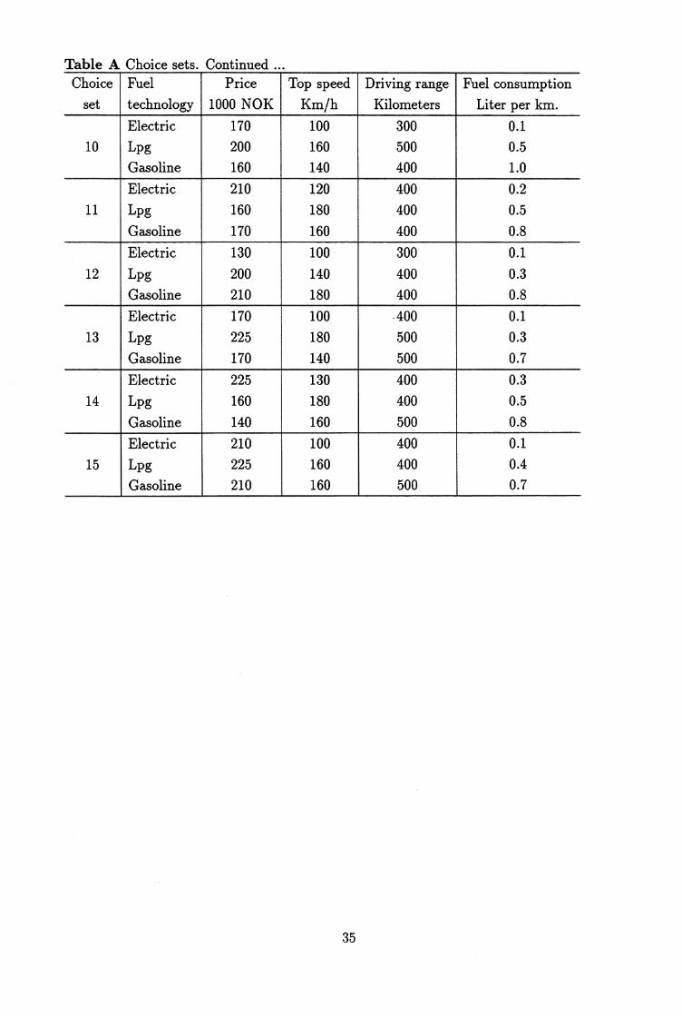
A Choice sets. Continued ...Choice

setFuel

technology

Price

1000 NOK

Top speed

Km/h

Driving range

Kilometers

Fuel consumption

Liter per km.

Electric 170 100 300 0.110 Lpg 200 160 500 0.5

Gasoline 160 140 400 1.0

Electric 210 120 400 0.211 Lpg 160 180 400 0.5

Gasoline 170 160 400 0.8

Electric 130 100 300 0.1

12 Lpg 200 140 400 0.3Gasoline 210 180 400 0.8

Electric 170 100 400 0.1

13 Lpg 225 180 500 0.3

Gasoline 170 140 500 0.7

Electric 225 130 400 0.3

14 Lpg 160 180 400 0.5

Gasoline 140 160 500 0.8

Electric 210 100 400 0.1

15 Lpg 225 160 400 0.4

Gasoline 210 160 500 0.7

35

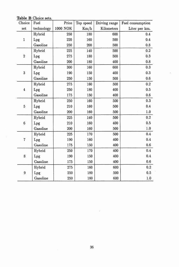
Table B Choice sets.Choice

set

Fuel

technology

Price

1000 NOK

Top speed

Km/h

Driving range

Kilometers

Fuel consumption

Liter per km.

Hybrid 250 180 600 0.4Lpg 220 160 500 0.4Gasoline 250 200 500 0.8

Hybrid 225 140 500 0.22 Lpg 275 180 500 0.3

Gasoline 200 180 400 0.8

Hybrid 300 160 600 0.3

3 Lpg 190 150 400 0.3

Gasoline 250 150 500 0.6

Hybrid 275 160 500 0.2

4 Lpg 250 180 400 0.5

Gasoline 175 150 400 0.6

Hybrid 250 160 500 0.3

5 Lpg 210 160 500 0.4

Gasoline 200 160 500 1.0

Hybrid 225 140 500 0.2

6 Lpg 210 160 400 0.5

Gasoline 200 160 500 1.0

Hybrid 225 170 500 0.4

7 Lpg 190 160 400 0.4

Gasoline 175 150 400 0.6

Hybrid 250 170 400 0.4

Lpg 190 150 400 0.4

Gasoline 175 150 400 0.6

Hybrid 275 160 600 0.2

9 Lpg 250 180 500 0.5

Gasoline 250 180 600 1.0

36

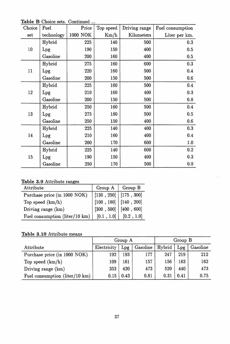
Table B Choice sets. ContinuedChoice

setFueltechnology

Price

1000 NOK

Top speed

Km/h

Driving rangeKilometers

Fuel consumptionLiter per km.

Hybrid 225 140 500 0.310 Lpg 190 150 400 0.5

Gasoline 200 160 400 0.5

Hybrid 275 160 600 0.311 Lpg 220 160 500 0.4

Gasoline 200 150 500 0.6

Hybrid 225 160 500 0.4

12 Lpg 210 160 400 0.3Gasoline 200 150 500 0.8

Hybrid 250 160 500 0.4

13 Lpg 275 180 500 0.5

Gasoline 250 150 400 0.6

Hybrid 225 140 400 0.3

14 Lpg 210 160 400 0.4

Gasoline 200 170 600 1.0

Hybrid 225 140 600 0.2

15 Lpg 190 150 400 0.3

Gasoline 250 170 500 0.8

Table 3.9 Attribute rangesAttribute

Purchase price (in 1000 NOK)Top speed (km/h)

Driving range (km)

Fuel consumption (liter/10 km)

Group A

[130 , 250][100 , 180]

[300 , 500][0.1 , 1.0]

Group B[175 , 300]

[140 , 200]

[400 , 600]

[0.2 , 1.0]

Table 3.10 Attribute meansGroup A

Electricity

192

109

3530.15

Lpg

193

161420

0.43

Attribute

Purchase price (in 1000 NOK)

Top speed (km/h)

Driving range (km)Fuel consumption (liter/10 km)

Gasoline

177

157473

0.81

Hybrid

247

156

520

0.31

Group

Lpg

219

163440

0.41

BGasoline

212

162

473

0.75

37

Kort lA

Ta hensyn til følgende informasjon når du vurderer alternativene:

1. Oppladningstiden for et tomt (flatt) batteri i en el-bil vil være ca. 3-4 timer når enbenytter en vanlig stikkontakt. Det eksisterer i dag teknologi som gjør det mulig åfullade et tomt batteri på 20 minutter. Dette må gjøres ved spesielle ladestasjoner(bensinstasjoner) .

2. El-bilen det her er snakk om er ikke nødvendigvis av samme type som de som er på

markedet idag.

3. Med kjørelengde for el-biler menes hvor langt man kan kjøre på et fullt ladet batteri

fa man må lade opp batteriet på el-bilen igjen. For bensin og gass drevne biler erdette lik den distansen man kan kjøre på en full tank (bide by- og landeveiskjøring).

4. Drivstoff kostnader pr. mil er regnet i liter bensin pr. mil. For el-bil er el-kostnadenepr. mil (inkludert batteri skift) omregnet til liter bensin pr. mil. Tilsvarende er

kostnadene pr. mil for gassbilen omregnet i liter bensin pr. mil.

5. Gassbilen forurenser mindre enn en bensinbil med katalysator. Bruk som utgangspunkt

at tilgjengeligheten på gass vil være den samme som for bensin i fremtiden.

6. Om bilen er drevet av bensin, gass eller elektrisitet har ingen betydning for bilens

størrelse, utseende eller levetid.

Kort 1B

Ta hensyn til følgende informasjon når du vurderer alternativene:

1. Gassbilen forurenser mindre enn en bensinbil med katalysator. Bruk som utgangspunkt

at tilgjengeligheten på gass vil være den samme som for bensin i fremtiden.

2. En hybrid bil er en el-bil som har et diesel/bensin aggregat som kan lade bilens batteri

under kjøring. Batteriet på bilen kan også lades opp på vanlig måte som f.eks. via

motorvarmer uttak. Hybridbilen omregnet i liter bensin pr. mil.

3. Drivstoff kostnader pr. mil er regnet i liter bensin pr. mil. For hybridbilen er kost-

nadene pr. mil (inkludert batteriskift) omregnet til liter bensin pr. mil. Tilsvarende

er kostnadene pr. mil for gassbilen omregnet i liter bensin pr. mil

4. Om bilen er drevet av bensin, gass eller elektrisitet har ingen betydning for bilens

størrelse, utseende eller levetid.

38

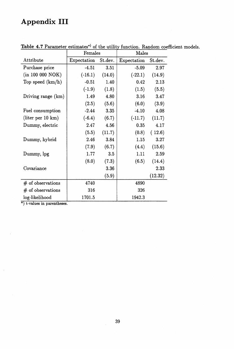
-4.51(-16.1)

-0.51

(-1.9)

1.49

(2.5)-2.44

(-6.4)

2.47

(5.5)2.46(7.9)

1.77

(8.0)

3.51(14.0)

1.40

(1.8)

4.80

(5.6)3.35

(6.7)

4.56(11.7)

3.84(6.7)

3.5

(7.3)

3.36

(5.9)

Appendix III

Table 4.7 Parameter estimates*) of the utility

Expectation St.dev.

4740316

1701.5

FemalesAttribute

Purchase price

(in 100 000 NOK)Top speed (km/h)

Driving range (km)

Fuel consumption(liter per 10 km)

Dummy, electric

Dummy, hybrid

Dummy, lpg

Covariance

# of observations# of observations

log-likelihood*) t-values in parentheses.

function. Random coefficient models.Males

Expectation St.dev.

-5.09 2.97

(-22.1) (14.9)

0.42 2.13

(1.5) (5.5)

3.16 3.47

(6.0) (3.9)-4.10 4.08

(-11.7) (11.7)

0.35 4.17

(0.8) ( 12.6)

1.15 3.27

(4.4) (15.6)

1.11 2.59

(6.5) (14.4)

2.33

(12.32)

4890326

1942.3

39

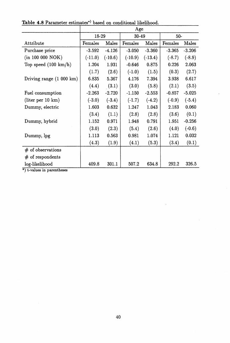
Table 4.8 Parameter estimates*) based on conditional likelihood.Age


Purchase price -3.592 -4.126 -3.050 -3.360 -3.365 -3.206(in 100 000 NOK) (-11.0) (-10.6) (-10.9) (-13.4) (-8.7) (-8.9)Top speed (100 km/h) 1.204 1.931 -0.646 0.875 0.226 2.063

(1.7) (2.6) (-1.0) (1.5) (0.3) (2.7)

Driving range (1 000 km) 6.835 5.367 4.176 7.394 3.938 6.617(4.4) (3.1) (3.0) (5.8) (2.1) (3.5)

Fuel consumption -2.263 -2.720 -1.150 -2.553 -0.857 -5.025

(liter per 10 km) (-3.0) (-3.4) (-1.7) (-4.2) (-0.9) (-5.4)Dummy, electric 1.603 0.632 1.247 1.043 2.183 0.060

(3.4) (1.1) (2.8) (2.8) (3.6) (0.1)

Dummy, hybrid 1.152 0.971 1.948 0.791 1.951 -0.256

(3.0) (2.3) (5.4) (2.6) (4.0) (-0.6)

Dummy, lpg 1.113 0.563 0.981 1.074 1.121 0.032

(4.3) (1.9) (4.1) (5.3) (3.4) (0.1)

# of observations

# of respondents

log-likelihood 409.8 301.1 507.2 634.8 292.2 326.5t-values in parentheses

40

Issued in the series Discussion Papers

42 R. Aaberge, O. Kravdal and T. Wennemo (1989): Un-observed Heterogeneity in Models of Marriage Dis-solution.

43 K.A. Mork, H.T. Mysen and O. Olsen (1989): BusinessCycles and Oil Price Fluctuations: Some evidence for sixOECD countries.

44 B. Bye, T. Bye and L. Lorentsen (1989): SIMEN. Stud-ies of Industry, Environment and Energy towards 2000.

45 0. Bjerkholt, E. Gjelsvit and O. Olsen (1989): GasTrade and Demand in Northwest Europe: Regulation,Bargaining and Competition.

46 L.S. Stambøl and K.O. Sørensen (1989): MigrationAnalysis and Regional Population Projections.

47 V. Christiansen (1990): A Note on the Short Run VersusLong Run Welfare Gain from a Tax Reform.

48 S. Glomsrød, H. Vennemo and T. Johnsen (1990): Sta-bilization of Emissions of CO2: A Computable GeneralEquilibrium Assessment.

49 J. Aasness (1990): Properties of Demand Functions forLinear Consumption Aggregates.

50 J.G. de Leon (1990): Empirical EDA Models to Fit andProject Time Series of Age-Specific Mortality Rates.

51 J.G. de Leon (1990): Recent Developments in ParityProgression Intensities in Norway. An Analysis Based onPopulation Register Data

52 R. Aaberge and T. Wennemo (1990): Non-StationaryInflow and Duration of Unemployment

53 R. Aaberge, J.K. Dagsvik and S. Strøm (1990): LaborSupply, Income Distribution and Excess Burden ofPersonal Income Taxation in Sweden

54 R. Aaberge, J.K. Dagsvik and S. Strøm (1990): LaborSupply, Income Distribution and Excess Burden ofPersonal Income Taxation in Norway

55 H. Vennemo (1990): Optimal Taxation in Applied Ge-neral Equilibrium Models Adopting the AnningtonAssumption

56 N.M. Stolen (1990): Is there a NAIRU in Norway?

57 A. Cappelen (1991): Macroeconomic Modelling: TheNorwegian Experience

58 J.K. Dagsvik and R. Aaberge (1991): HouseholdProduction, Consumption and Time Allocation in Pau

59 R. Aaberge and J.K. Dagsvik (1991): Inequality inDistribution of Hours of Work and Consumption in Peru

60 T.J. Klette (1991): On the Importance of R&D andOwnership for Productivity Growth. Evidence fromNorwegian Micro-Data 1976-85

61 K.H. Alfsen (1991): Use of Macroeconomic Models inAnalysis of Environmental Problems in Norway andConsequences for Environmental Statistics

62 H. Vennemo (1991): An Applied General EquilibriumAssessment of the Marginal Cost of Public Funds inNorway

63 H. Vennemo (1991): The Marginal Cost of PublicFunds: A Comment on the Literature

64 A. Brendemoen and H. Vennemo (1991): A climateconvention and the Norwegian economy: A CGE as-sessment

65 K.A. Brekke (1991): Net National Product as a WelfareIndicator

66 E. Bowitz and E. Storm (1991): Will Restrictive De-mand Policy Improve Public Sector Balance?

67 A. Cappelen (1991): MODAG. A Medium TermMacroeconomic Model of the Norwegian Economy

68 B. Bye (1992): Modelling Consumers' Energy Demand

69 K.H. Alfsen, A. Brendemoen and S. Glomsrød (1992):Benefits of Climate Policies: Some Tentative Calcula-tions

70 R. Aaberge, Xiaojie Chen, Jing Li and Xuezeng Li(1992): The Structure of Economic Inequality amongHouseholds Living in Urban Sichuan and Liaoning,1990

71 K.H. Alfsen, K.A. Brekke, F. Brunvoll, H. Lurås, K.Nyborg and H.W. Sæbø (1992): Environmental Indi-cators

72 B. Bye and E. Holmøy (1992): Dynamic EquilibriumAdjustments to a Terms of Trade Disturbance

73 0. Aukrust (1992): The Scandinavian Contribution toNational Accounting

74 J. Aasness, E. Eide and T. Skjerpen (1992): A Crimi-nometric Study Using Panel Data and Latent Variables

75 R. Aaberge and Xuezeng Li (1992): The Trend inIncome Inequality in Urban Sichuan and Liaoning,1986-1990

76 J.K. Dagsvik and S. Strøm (1992): Labor Supply withNon-convex Budget Sets, Hours Restriction and Non-pecuniary Job-attributes

77 J.K. Dagsvik (1992): Intertemporal Discrete Choice,Random Tastes and Functional Form

78 H. Vennemo (1993): Tax Reforms when Utility isComposed of Additive Functions

79 J.K. Dagsvik (1993): Discrete and Continuous Choice,Max-stable Processes and Independence from IrrelevantAttributes

80 J.K. Dagsvik (1993): How Large is the Class of Gen-eralized Extreme Value Random Utility Models?

81 H. Birkelund, E. Gjelsvik, M. Aaserud (1993): Carbon/energy Taxes and the Energy Market in WesternEurope

82 E. Bowitz (1993): Unemployment and the Growth in theNumber of Recipients of Disability Benefits in Norway

83 L. Andreassen (1993): Theoretical and EconometricModeling of Disequilibrium

84 K.A. Brekke (1993): Do Cost-Benefit Analyses favourEnvironmentalists?

85 L. Andreassen (1993): Demographic Forecasting with aDynamic Stochastic Microsimulation Model

86 G.B. Asheim and K.A. Brekke (1993): Sustainabilitywhen Resource Management has Stochastic Conse-quences

87 0. Bjerkholt and Yu Zhu (1993): Living Conditions ofUrban Chinese Households around 1990

88 R. Aaberge (1993): Theoretical Foundations of LorenzCurve Orderings

89 J. Aasness, E. Sian and T. Skjerpen (1993): EngelFunctions, Panel Data, and Latent Variables - withDetailed Results

41

90 I. Svendsen (1993): Testing the Rational ExpectationsHypothesis Using Norwegian Microeconornic DataTesting the REH. Using Norwegian MicroeconomicData

91 E. Bowitz, A. Rodseth and E. Storm (1993): FiscalExpansion, the Budget Deficit and the Economy: Nor-way 1988-91

92 R. Aaberge, U. Colombino and S. Strom (1993): LaborSupply in Italy

93 T.J. Klette (1993): Is Price Equal to Marginal Costs? AnIntegrated Study of Price-Cost Margins and ScaleEconomies among Norwegian Manufacturing Estab-lishments 1975-90

94 J.K. Dagsvik (1993): Choice Probabilities and Equili-brium Conditions in a Matching Market with FlexibleContracts

114 K.E. Rosenciahl (1994): Does Improved EnvironmentalPolicy Enhance Economic Growth? Endogenous GrowthTheory Applied to Developing Countries

115 L. Andreassen, D. Fredriksen and O. Ljones (1994): TheFuture Burden of Public Pension Benefits. AMicrosimulation Study

116 A. Brendemoen (1994): Car Ownership Decisions inNorwegian Households.

117 A. Langorgen (1994): A Macromodel of LocalGovernment Spending Behaviour in Norway

118 K.A. Brekke (1994): Utilitarism, Equivalence Scales andLogarithmic Utility

119 K.A. Brekke, H. Lulls and K. Nyborg (1994): SufficientWelfare Indicators: Allowing Disagreement inEvaluations of Social Welfare

120 Ti. Klette (1994): R&D, Scope Economies and Com-pany Structure: A "Not-so-Fixed Effect" Model of PlantPerformance

95 T. Komstad (1993): Empirical Approaches for Ana-lysing Consumption and Labour Supply in a Life CyclePerspective

96 T. Kornstad (1993): An Empirical Life Cycle Model of 121

Savings, Labour Supply and Consumption withoutIntertemporal Separability 122

97 S. Kvemdokk (1993): Cogitions and Side Payments inInternational CO2 Treaties 123

98 T. Eika (1993): Wage Equations in Macro Models.Phillips Curve versus Error Correction Model Deter- 124mination of Wages in Large-Scale UK Macro Models

99 A. Brendemoen and H. Vennemo (1993): The MarginalCost of Funds in the Presence of External Effects 125

100 K.-G. Lindquist (1993): Empirical Modelling ofNorwegian Exports: A Disaggregated Approach

101 A.S. Jore, T. Skjerpen and A. Rygh Swensen (1993): 126

Testing for Purchasing Power Parity and Interest RateParities on Norwegian Data 127

102 R. Nesbalcken and S. Strom (1993): The Choice of SpaceHeating System and Energy Consumption in NorwegianHouseholds (Will be issued later) 128

103 A. Aaheim and K. Nyborg (1993): "Green NationalProduct": Good Intentions, Poor Device? 129

104 K.H. Alfsen, H. Birkelund and M. Aaserud (1993):Secondary benefits of the EC Carbon/ Energy Tax

105 J. Aasness and B. Holtsmark (1993): Consumer Demandin a General Equilibrium Model for EnvironmentalAnalysis

106 K.-G. Lindquist (1993): The Existence of Factor Sub-stitution in the Primary Aluminium Industry: A Multi-variate Error Correction Approach on Norwegian PanelData

107 S. Kvemdokk (1994): Depletion of Fossil Fuels and theImpacts of Global Warming

108 K.A. Magnussen (1994): Precautionary Saving and Old-Age Pensions

109 F. Johansen (1994): Investment and Financial Con-straints: An Empirical Analysis of Norwegian Firms

110 K.A. Brekke and P. Boring (1994): The Volatility of OilWealth under Uncertainty about Parameter Values

111 MJ. Simpson (1994): Foreign Control and NorwegianManufacturing Performance

112 Y. Willassen and T.J. Klette (1994): Correlated 137Measurement Errors, Bound on Parameters, and a Modelof Producer Behavior 138

113 D. Wetterwald (1994): Car ownership and private caruse. A microeconometric analysis based on Norwegiandata 139

Y. Willassen (1994): A Generalization of Hall's Speci-fication of the Consumption function

E. Holmøy, T. Hægeland and 0. Olsen (1994): EffectiveRates of Assistance for Norwegian Industries

K. Mohn (1994): On Equity and Public Pricing inDeveloping Countries

J. Aasness, E. Eide and T. Skjerpen (1994): Crimi-nometrics, Latent Variables, Panel Data, and DifferentTypes of Crime

E. ikon and Ti. Klette (1994): Errors in Variables andPanel Data: The Labour Demand Response to PermanentChanges in Output

I. Svendsen (1994): Do Norwegian Firms FormExtrapolative Expectations?

TJ. Klette and Z. Griliches (1994): The Inconsistency ofCommon Scale Estimators when Output Prices areUnobserved and Endogenous

K.E. Rosendahl (1994): Carbon Taxes and the PetroleumWealth

L. Andreassen (1995): A Framework for EstimatingDisequilibrium Models with Many Markets

L. Andreassen (1995): Aggregation when Markets do notClear

S. Johansen and A. Rygh Swensen (1994): TestingRational Expectations in Vector Autoregressive Models

130 Ti. Klette (1994): Estimating Price-Cost Margins andScale Economies from a Panel of Microdata

131 L. A. Grünfeld (1994): Monetary Aspects of BusinessCycles in Norway: An Exploratory Study Based onHistorical Data

132 K.-G. Lindquist (1994): Testing for Market Power in theNorwegian Primary Aluminium Industry

133 T. J. Klette (1994): R&D, Spillovers and Performanceamong Heterogenous Firms. An Empirical Study UsingMicrodata

134 K.A. Brekke and H.A. Gravningsmyhr (1994): AdjustingNNP for instrumental or defensive expenditures. Ananalytical approach

135 T.O. Thoresen (1995): Distributional and BehaviouralEffects of Child Care Subsidies

136 T. J. Klette and A. Mathiassen (1995): Job Creation, JobDestruction and Plant Turnover in NorwegianManufacturing

K. Nyborg (1995): Project Evaluations and DecisionProcesses

42

140 T. Skjerpen (1995): Is there a Business Cycle Com-ponent in Norwegian Macroeconomic Quarterly TimeSeries?

141 J.K. Dagsvik (1995): Probabilistic Choice Models forUncertain Outcomes

142 M. Rønsen (1995): Maternal employment in Norway, Aparity-specific analysis of the return to full-time andpart-time work after birth

143 A. Bruvoll, S. Glomsrød and H. Vennemo (1995): TheEnvironmental Drag on Long- term Economic Perfor-mance: Evidence from Norway

144 T. Bye and T. A. Johnsen (1995): Prospects for a Corn-mon, Deregulated Nordic Electricity Market

145 B. Bye (1995): A Dynamic Equilibrium Analysis of aCarbon Tax

146 T. O. Thomsen (1995): The Distributional Impact of theNorwegian Tax Reform Measured by Disproportionality

147 E. Holmoy and T. Hægeland (1995): Effective Rates ofAssistance for Norwegian Industries

148 J. Aasness, T. Bye and H.T. Mysen (1995): WelfareEffects of Emission Taxes in Norway

149 J. Aasness, E. Non and Terje Skjerpen (1995):Distribution of Preferences and Measurement Errors in aDisaggregated Expenditure System

150 E. Bowitz, T. Fæhn, L. A. Grünfeld and K. Mourn(1995): Transitory Adjustment Costs and Long TermWelfare Effects of an EU-membership — The NorwegianCase

151 I. Svendsen (1995): Dynamic Modelling of DomesticPrices with Time-varying Elasticities and RationalExpectations

152 I. Svendsen (1995): Forward- and Backward LookingModels for Norwegian Export Prices

153 A. Langorgen (1995): On the SimultaneousDetermination of Current Expenditure, Real Capital, FeeIncome, and Public Debt in Norwegian LocalGovernment

154 A. Katz and T. Bye(1995): Returns to Publicly OwnedTransport Infrastructure Investment. A CostFunction/Cost Share Approach for Norway, 1971-1991

155 K. O. Aarbu (1995): Some Issues About the NorwegianCapital Income Imputation Model

156 P. Boug, K. A. Mork and T. Tjemsland (1995): FinancialDeregulation and Consumer Behavior: the NorwegianExperience

157 B. E. Naug and R. Nymoen (1995): Import PriceFormation and Pricing to Market: A Test on NorwegianData

158 R. Aaberge (1995): Choosing Measures of Inequality forEmpirical Applications.

159 T. J. Klette and S. E. Forre: Innovation and Job Creationin a Small Open Economy: Evidence from NorwegianManufacturing Plants 1982-92

160 S. Holden, D. Kolsrud and B. Vikomn (1995): NoisySignals in Target Zone Regimes: Theory and MonteCarlo Experiments

161 T. Hægeland (1996): Monopolistic Competition,Resource Allocation and the Effects of Industrial Policy

162 S. Grepperud (1996): Poverty, Land Degradation andClimate Uncertainty

163 S. Grepperud (1996): Soil Conservation as an Investmentin Land

164 K. A. Brekke, V. Iversen and J. Aune (1996): SoilWealth in Tanzania

165 J..K. Dagsvik, D.G. Wetterwald and R. Aaberge (1996):Potential Demand for Alternative Fuel Vehicles

43

Discussion Papers

Statistics NorwayResearch DepartmentP.O.B. 8131 Dep.N-0033 Oslo

Tel.: +47-22 86 45 00Fax: + 47 - 22 11 12 38

ISSN 0803-074X

OW11110 Statistics Norway Research Department