Post-emplacement dynamics of andesitic lava flows at Volcán ...

HAL Id: hal-03480697https://hal.archives-ouvertes.fr/hal-03480697

Submitted on 20 Dec 2021

HAL is a multi-disciplinary open accessarchive for the deposit and dissemination of sci-entific research documents, whether they are pub-lished or not. The documents may come fromteaching and research institutions in France orabroad, or from public or private research centers.

L’archive ouverte pluridisciplinaire HAL, estdestinée au dépôt et à la diffusion de documentsscientifiques de niveau recherche, publiés ou non,émanant des établissements d’enseignement et derecherche français ou étrangers, des laboratoirespublics ou privés.

Distributed under a Creative Commons Attribution - NonCommercial| 4.0 InternationalLicense

Post-emplacement dynamics of andesitic lava flows atVolcán de Colima, Mexico, revealed by radar and optical

remote sensing dataAlexandre Carrara, Virginie Pinel, Pascale Bascou, Emmanuel Chaljub,

Servando de La Cruz-Reyna

To cite this version:Alexandre Carrara, Virginie Pinel, Pascale Bascou, Emmanuel Chaljub, Servando de La Cruz-Reyna.Post-emplacement dynamics of andesitic lava flows at Volcán de Colima, Mexico, revealed by radarand optical remote sensing data. Journal of Volcanology and Geothermal Research, Elsevier, 2019,381, pp.1 - 15. �10.1016/j.jvolgeores.2019.05.019�. �hal-03480697�

p. 1

Post-emplacement dynamics of andesitic lava flows at 1

Volcán de Colima, Mexico, revealed by radar and optical 2

remote sensing data 3

Alexandre Carrara1*, Virginie Pinel1, Pascale Bascou1, Emmanuel Chaljub1, Servando De 4

la Cruz-Reyna2 5

1 Univ. Grenoble Alpes, Univ. Savoie Mont Blanc, CNRS, IRD, IFSTTAR, ISTerre, 38000 Grenoble, 6

France 7

2 Instituto de Geofisica, Universidad Nacional Autónoma de Mexico, CDMX 04510, 8

Mexico 9

* Corresponding author: Alexandre Carrara ([email protected])10

11

12

Highlights:-We propose a novel approach for retrieving a 3D displacement field on lava 13

flows. 14

-We measure horizontal motion on a lava flow several months after its emplacement.15

-Thermal contraction, loading and flow all contribute to the displacements.16

17

© 2019 published by Elsevier. This manuscript is made available under the CC BY NC user licensehttps://creativecommons.org/licenses/by-nc/4.0/

Version of Record: https://www.sciencedirect.com/science/article/pii/S0377027319301076Manuscript_cb4764edd3812640c0867260969b8a00

p. 2

Abstract : 281 words ; Main text : 9510 words, 4 tables, 11 figures, 65 references 18

Abstract: 19

We used optical and radar remote sensing datasets to map, estimate the volume, and 20

measure the surface displacements of lava flows emplaced on the flanks of Volcán de Colima, 21

Mexico by extrusion of lava dome material from the end of 2014 to early 2016. Our main result 22

is that the flow motion of the lava contributes significantly to the recorded displacements 23

several months after its emplacement. First, we mapped the deposits and estimated their 24

volumes using two Digital Elevation Models (DEM), one derived from radar data acquired before 25

the peak of activity and one derived from optical images acquired just after this peak of activity. 26

Coherence information derived from the radar dataset added some temporal constraints on the 27

timing of emplacement of various deposits. We thus estimated a mean extrusion rate of 1-2 m3 28

s-1 between November 2014 and February 2015. We then used a new approach to reconstruct 29

the 3D displacement field, taking advantage of images acquired by the same satellite, on both 30

ascending and descending tracks, and using a physical a priori on the direction of horizontal 31

displacements. Our results show that about 2 cm yr-1 of horizontal motion is still recorded a few 32

months after the emplacement on the SW lava flow, which is the only one covered by the two-33

acquisition geometries. In order to differentiate the potential causes of the observed 34

displacements, we modeled the thermal contraction of the lava flow using a finite element 35

numerical method. Removing the contribution of thermoelastic contraction from the measured 36

displacements enable to infer both the viscoelastic loading and flow motion effects from the 37

residuals. Results show that, thermal contraction, flow motion and viscoelastic loading 38

contribute significantly to the displacements recorded. 39

p. 3

Keywords: 40

- Remote sensing, InSAR, 3D displacement field, lava flow, subsidence, thermal contraction. 41

42

43

1. Introduction: 44

Spaceborne remote sensing datasets, providing information with a good spatial coverage 45

over areas that are difficult to access, have proven to be powerful tools to study lava flows. 46

Radar images have the advantage that they are insensitive to cloud cover and solar lighting. 47

They can be used to detect and map new lava flows with either coherence or amplitude based 48

methods (Schaber et al., 1980; Zebker et al., 1987, 1996; Gaddis, 1992; Rowland et al., 2003; 49

Dietterich et al., 2012). They are also commonly used to estimate their thickness and volume, 50

and thus determine volcano extrusion rates (Stevens et al., 1999; Rowland et al., 2003; Terunuma, et 51

al., 2005; Poland, 2014; Bato et al., 2016; Arnold et al., 2017), which is key information in terms of 52

hazard assessment. Interferometry has been used to study the post-emplacement dynamics of 53

lava flows (e.g. Briole et al., 1997; Lu et al., 2005; Ebmeier et al., 2012; Bato et al., 2016; 54

Chaussard, 2016, see table 1), and in turn, calculate their material properties (Wittmann et al., 55

2017). However, most of these studies were performed on basaltic lava flows emplaced on 56

gentle topographic slopes (see table 1), where lava flows are frequent and InSAR is highly 57

effective. On the contrary, it is well-established that InSAR methods are more difficult to use on 58

andesitic stratovolcanoes because of their steep topography and generally dense vegetation 59

coverage, causing low coherence and noisy data (Pinel et al., 2011). A limitation to the use of 60

InSAR to characterize post-emplacement deformation of lava flows is that, in the absence of 61

p. 4

additional measurements of the surface displacement such as GNSS or SAR acquired from a 62

different satellite (Peltier et al., 2017), radar images acquired by a given satellite for both the 63

ascending and descending tracks are difficult to use to reconstruct the 3D displacement fields 64

due to the lower accuracy in the north‒south (N‒S) direction (InSAR measurements being only 65

sensitive to the displacements along the satellite line of sight, which horizontal projection is 66

usually close to the east-west direction for both ascending and descending tracks). Thus, most 67

studies consider that the Line of Sight (LOS) displacements measured result from vertical 68

displacements alone. This assumption prevents the extraction of information about the lava 69

flows horizontal displacement fields being extracted, and could introduce an error into the 70

estimated vertical displacements. 71

Volcán de Colima, one of the most active volcanoes in North America, is located at the 72

SW front of the Trans Mexican Volcanic Belt (Fig. 1), created by the subduction of the Cocos and 73

Rivera plates under the North American plate. Volcanic activity is characterized by cycles of 74

around one hundred years which culminate in a large Plinian eruption; the last major explosive 75

eruption was in 1913 (Robin et al., 1987; Luhr and Carmichael, 1990). 76

A new episode of mostly effusive activity began in 1961, when the lava that had slowly 77

infilled the crater left by the 1913 explosions reached the lowest notch in the northern crater 78

rim, generating block-lava flows. Similar episodes of activity followed in 1975-1976 and 1981-79

1982. In 1991 the lava extrusion began to form a lava dome that fed new block-lava flows (Luhr, 80

2002). Collapses of the crater rim and the overflowing dome have since caused numerous block 81

and ash flows, particularly in 2004-2005. Dome-building activity resumed in 2007. Vulcanian 82

p. 5

explosions destroyed the dome in early 2013, and a new dome began growing again overflowing 83

from the crater and producing further lava flows in March 2013 (Capra et al, 2016). 84

At the end of 2014, an increase in eruptive activity was recorded, notably marked by the 85

July 10 and 11, 2015 pyroclastic density currents (PDCs) which represented the largest runout 86

since 1913 (Capra et al., 2016; Reyes-Dávila et al., 2016; Macorps et al., 2017). The 2015 87

eruption was not preceded by any detectable precursors in terms of edifice inflation or seismic 88

velocity variations (Lesage et al., 2018). Before and after these events, large lava flows were 89

emplaced on the volcano flanks (Reyes-Dávila et al., 2016). Activity reports describe active lava 90

flows on the western (W) and south‒western (SW) flanks from September‒November 2014 to 91

mid‒February 2015, when no downward motion was observed (Sennert, 2015a). In July, 2015, 92

just after the PDC occurrences, another lava flow formed on the southern (S) flank in the same 93

channel as the PDCs (Sennert, 2015b). Most of studies about this high activity period deal with 94

PDC deposits (Capra et al., 2016; Reyes-Dávila et al., 2016; Macorps et al., 2017) but lava flows 95

should also be considered in order to properly characterize and understand the volcano activity. 96

The present study combines both radar and optical remote sensing data with the aim of 97

determining where lava flows were emplaced as well as their volumes and their post-98

emplacement dynamics, in order to have greater insight into the 2014-2015 eruptive crisis of 99

Volcán de Colima. New approaches are proposed to: (1) improve the remote sensing detection 100

of lava flows on andesitic stratovolcanoes, and (2) reconstruct approximate 3D ground 101

displacements associated with the emplacement of lava flows using InSAR LOS measurements 102

on both the ascending and descending tracks from a single satellite, without any other 103

additional observation. Finally, the thermal compaction of the lava flow is numerically modeled 104

p. 6

and its relative contribution together with the loading and downward flow effect, are 105

investigated. An estimation of the magma bulk viscosity is also derived based on the downward 106

lava displacement. 107

108

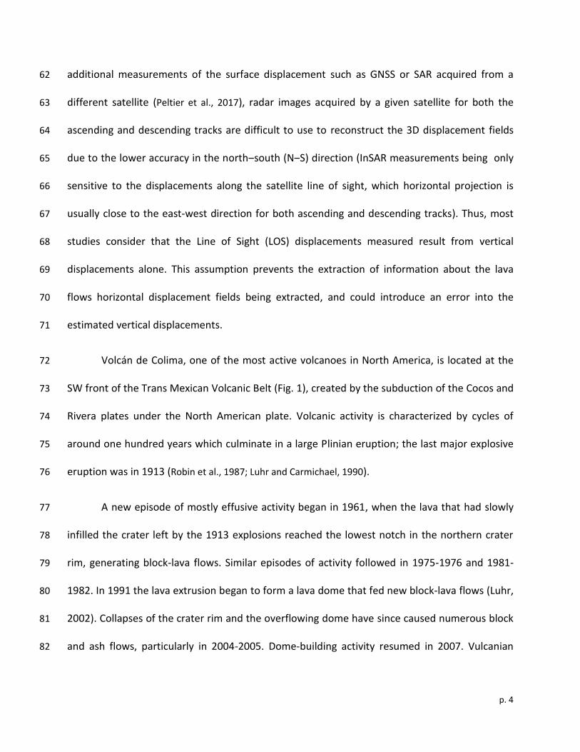
Figure 1: Map with footprints of optical and radar images used in this study. The red dashed line 109

marks the edge of the Trans Mexican Volcanic Belt (TMVB) (red area in the inset). The large 110

blue triangle shows the location of Volcán de Colima (CV). Green and blue rectangles are, 111

respectively, footprints of Sentinel-1A ascending (Orbit A49, sub‒swath 3) and descending 112

tracks (Orbit D12, sub‒swath 1) (for simplicity, only the bursts and sub‒swaths used are 113

delimited). The yellow rectangle delimits the extent of Tandem-X DEM. Inset shows the 114

p. 7

described area location (dashed blue rectangle) at a larger scale. The PLEIADES DEM coverage 115

(10×13 km2 centered on the edifice summit) is not displayed here for clarity. 116

117

118

Volcano (deposit year) Time span (yrs) Lava composition Local slope Ref

Africa

Fogo (1995) 3 Basaltic ~3° (Amelung and Day, 2002)

Piton de la Fournaise (1998‒2007) 2‒16 Basaltic ~17° (Chen et al., 2018)

(2010) 0.3‒3 Basaltic ~7° (Bato et al., 2016)

Mt Nyamuragira (2004‒2010) 0‒5.5 Basaltic ~4° (Samsonov and d’Oreye, 2012)

North America

Paricutin (1943‒1952) 55‒68 Basaltic-Andesitic ~5° (Chaussard, 2016)

(1943‒1952) 56‒65 Basaltic-Andesitic ~8° (Fournier et al., 2010)

Santiaguito (2004‒2005) 4‒6 Dacitic ~21° (Ebmeier et al., 2012)

Okmok (1958 & 1997) 0.5‒3.5 Basaltic ~1° (Lu et al., 2005)

Colima (1998) 4‒8 Andesitic ~25° (Pinel et al., 2011)

(2014‒2015) 0.5‒1.1 Andesitic ~18° This study

Pacaya (2010) 0.1‒4 Basaltic ~10° (Schaefer et al., 2016)

Europe

Etna (1986‒1987 & 1989) 3‒7 Basaltic ~23° (Briole et al., 1997)

(1991‒1993) 2‒6 Basaltic ~13° (Stevens et al., 2001)

Krafla (1975‒1984) 8‒20 Basaltic ~1° (Sigmundsson et al., 1997)

Hekla (1991 & 2000) 2‒25 Basaltic-Andesitic ~8° (Wittmann et al., 2017)

South America

Reventador (2002‒2005) 3‒6 Andesitic ~18° (Fournier et al., 2010)

Lonquinay (1988‒1989) 17‒18 Andesitic ~4° (Fournier et al., 2010)

p. 8

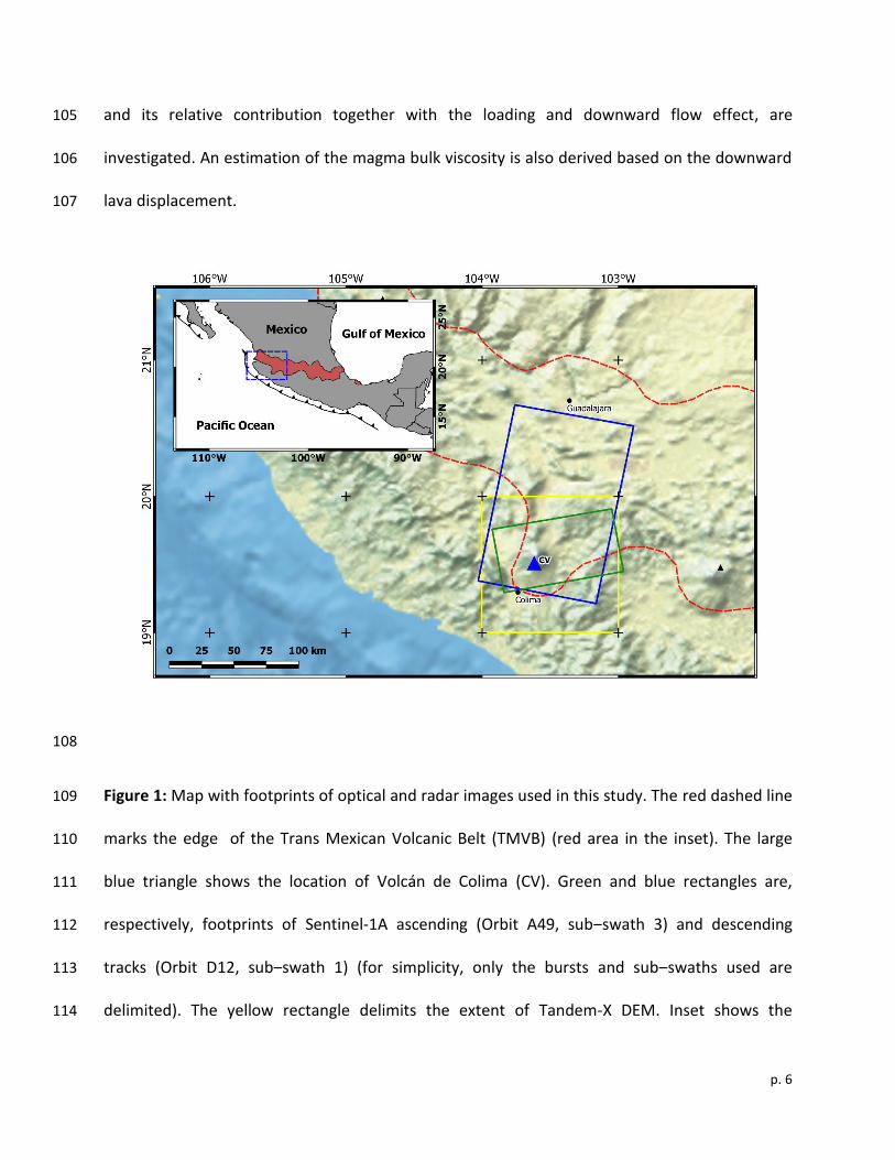
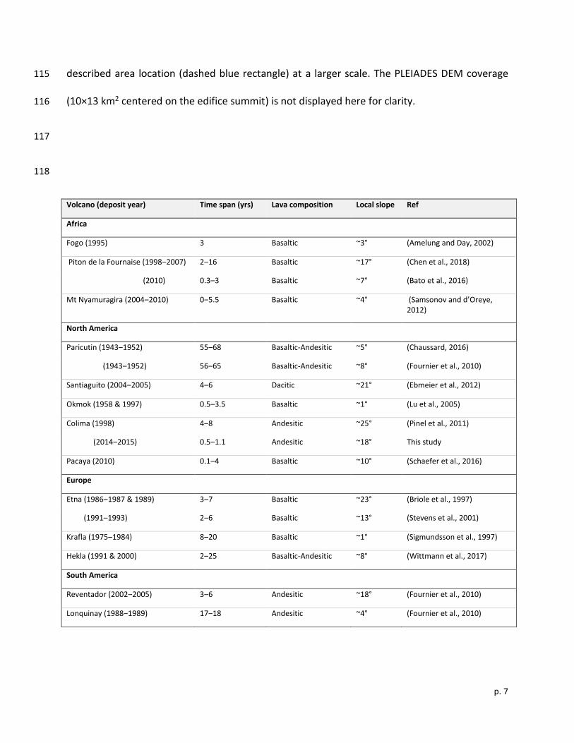
Table 1: List of the InSAR studies related to lava flow post-emplacement deformations. Local 119

slope was estimated from the SRTM DEM. Time span corresponds to the time lapse between 120

the lava flow emplacement and SAR image acquisition. 121

2. Data and methods 122

2.1. Data and processing 123

Topographic changes induced by lava flow emplacement were estimated based on two 124

Digital Elevation Models (DEM). The pre-eruptive DEM used is the TanDEM-X, 12 m resolution, 125

provided by the German Space Agency (©DLR 2015) and obtained from X-band radar images 126

acquired between January 2011 and August 2014 (see footprint on Fig. 1). A post-eruptive DEM 127

was obtained using one stereo pair of Pleiades optical images (©CNES_2016, distribution 128

AIRBUS DS, France, all rights reserved) acquired on 10 January 2016 and made available through 129

an ISIS (Incitation à l’utilisation Scientifique des Images Spot, French initiative to promote the 130

scientific use of Spot images) project. Pleiades panchromatic images have a nominal resolution 131

of 0.5m. Along-track incidence angles of the two images are -9.3° and -13.1°, while the across-132

track angle varies between -14.5° and -9.6°. The DEM was computed using the NASA open 133

source software Ames Stereo Pipeline (Broxton and Edwards, 2008). Disparities between the 134

two images are searched for; this provides a point cloud of the surface topography which is then 135

converted onto a grid regularly spaced every 3 m. In this way we obtain a Digital Surface Model, 136

but as no vegetation is present on the region of interest, where lava flows are emplaced, it 137

corresponds to a DEM. 138

p. 9

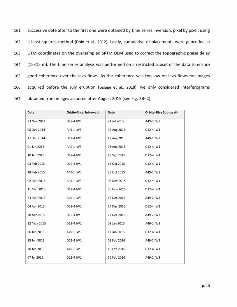
Surface displacements induced by the lava flows were quantified based on 36 SAR 139

images acquired from November 23, 2014 to February 10, 2016, on both ascending and 140

descending tracks, by the European satellite Sentinel-1A with a Vertical-Vertical polarization 141

(Table 2). Images were acquired in Terrain Observation by Progressive Scans SAR (TOPSAR) 142

Interferometric Wide Swath mode (Zan and Guarnieri, 2006) and provided as Single Look 143

Complex (SLC) images with a spatial resolution of 15.6 m in azimuth and 2.3 m in slant range 144

(see Fig. 2 for spatio-temporal distribution of the dataset). As Volcán de Colima’s flanks are 145

steep, local topographic slopes are close to or even greater than the incidence angle, inducing 146

low resolution and a possible layover effect on the flanks facing the satellite. This is particularly 147

true for the descending track where the incidence angle is very close to the volcano slope on the 148

eastern flanks around the summit area (~35°). Ground area affected by low resolution was 149

estimated and consequently masked based on acquisition geometries. 150

Interferograms as well as coherence images were computed on ascending and 151

descending tracks from SLC images using the NSBAS processing chain as described in Doin et al 152

(2012) and modified to allow for TOPSAR data ingestion (Grandin, 2015). Topographic phase 153

contribution was removed using the SRTM Digital Elevation Model at 30 m resolution 154

oversampled to 15 m. Interferograms were corrected for tropospheric phase delays using 155

atmospheric data provided by the European Center for Medium Range Weather Forecast 156

(ECMRWF) (Doin et al., 2009). Interferograms were then unwrapped using the ROI_PAC branch-157

cut unwrapping algorithm. Phase delays were converted to LOS ground displacements 158

considering ground displacement as null in a 255x255 m reference area located at the basal part 159

of the SW volcano sector (see Fig. 6‒7). Cumulative LOS ground displacements for each 160

p. 10

successive date after to the first one were obtained by time series inversion, pixel by pixel, using 161

a least squares method (Doin et al., 2012). Lastly, cumulative displacements were geocoded in 162

UTM coordinates on the oversampled SRTM DEM used to correct the topographic phase delay 163

(15×15 m). The time series analysis was performed on a restricted subset of the data to ensure 164

good coherence over the lava flows. As the coherence was too low on lava flows for images 165

acquired before the July eruption (Lesage et al., 2018), we only considered interferograms 166

obtained from images acquired after August 2015 (see Fig. 2B‒C). 167

Date Orbite-Slice Sub-swath Date Orbite-Slice Sub-swath

23 Nov 2014 D12-4 IW1 24 Jul 2015 A49-1 IW3

08 Dec 2014 A49-1 IW3 02 Aug 2015 D12-4 IW1

17 Dec 2014 D12-4 IW1 17 Aug 2015 A49-1 IW3

01 Jan 2015 A49-1 IW3 26 Aug 2015 D12-4 IW1

10 Jan 2015 D12-4 IW1 19 Sep 2015 D12-4 IW1

03 Feb 2015 D12-4 IW1 13 Oct 2015 D12-4 IW1

18 Feb 2015 A49-1 IW3 28 Oct 2015 A49-1 IW3

02 Mar 2015 A49-1 IW3 06 Nov 2015 D12-4 IW1

11 Mar 2015 D12-4 IW1 30 Nov 2015 D12-4 IW1

23 Mar 2015 A49-1 IW3 15 Dec 2015 A49-2 IW3

04 Apr 2015 D12-4 IW1 24 Dec 2015 D12-4 IW1

28 Apr 2015 D12-4 IW1 27 Dec 2015 A49-2 IW3

22 May 2015 D12-4 IW1 08 Jan 2016 A49-2 IW3

06 Jun 2015 A49-1 IW3 17 Jan 2016 D12-4 IW1

15 Jun 2015 D12-4 IW1 01 Feb 2016 A49-2 IW3

30 Jun 2015 A49-1 IW3 10 Feb 2016 D12-4 IW1

07 Jul 2015 D12-4 IW1 25 Feb 2016 A49-2 IW3

p. 11

Table 2: List of the Sentinel-1A SAR images used in this study. Information on the acquisition 168

geometry for each track is provided in Table 3. 169

170

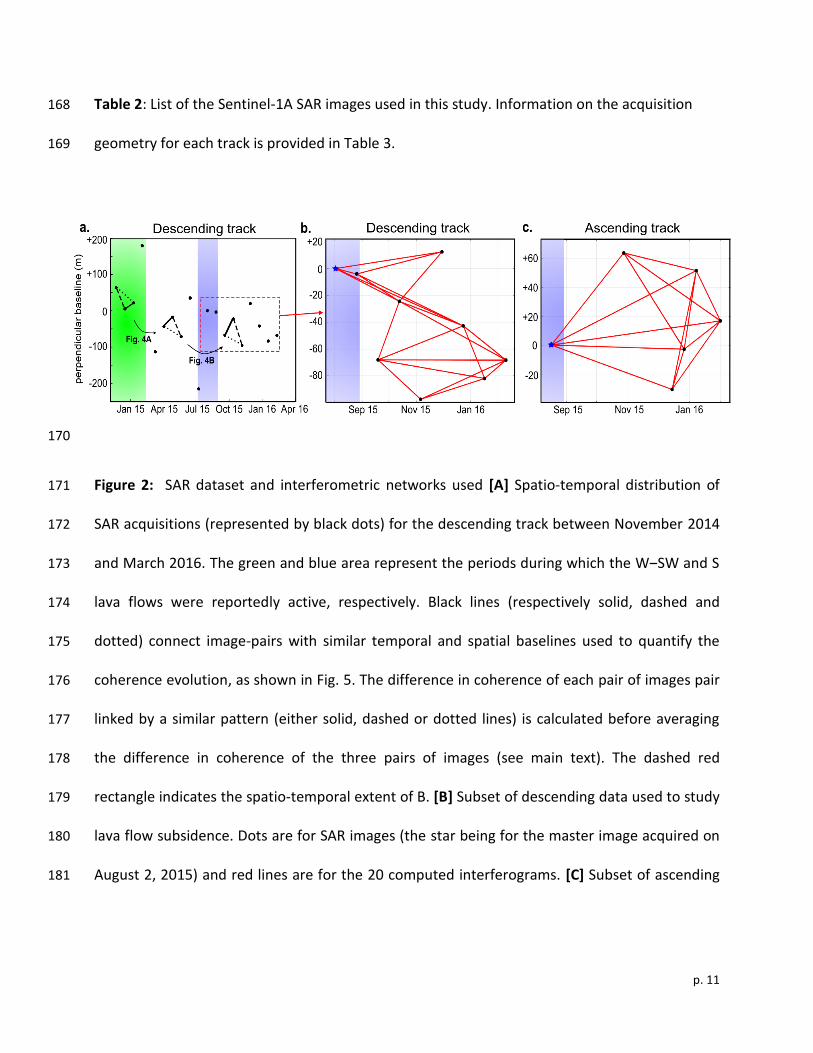
Figure 2: SAR dataset and interferometric networks used [A] Spatio-temporal distribution of 171

SAR acquisitions (represented by black dots) for the descending track between November 2014 172

and March 2016. The green and blue area represent the periods during which the W‒SW and S 173

lava flows were reportedly active, respectively. Black lines (respectively solid, dashed and 174

dotted) connect image-pairs with similar temporal and spatial baselines used to quantify the 175

coherence evolution, as shown in Fig. 5. The difference in coherence of each pair of images pair 176

linked by a similar pattern (either solid, dashed or dotted lines) is calculated before averaging 177

the difference in coherence of the three pairs of images (see main text). The dashed red 178

rectangle indicates the spatio-temporal extent of B. [B] Subset of descending data used to study 179

lava flow subsidence. Dots are for SAR images (the star being for the master image acquired on 180

August 2, 2015) and red lines are for the 20 computed interferograms. [C] Subset of ascending 181

p. 12

data used to study lava flow subsidence. Dots are for SAR images (the star being for the master 182

image acquired on August 17, 2015) and red lines are for the 14 computed interferograms. 183

184

185

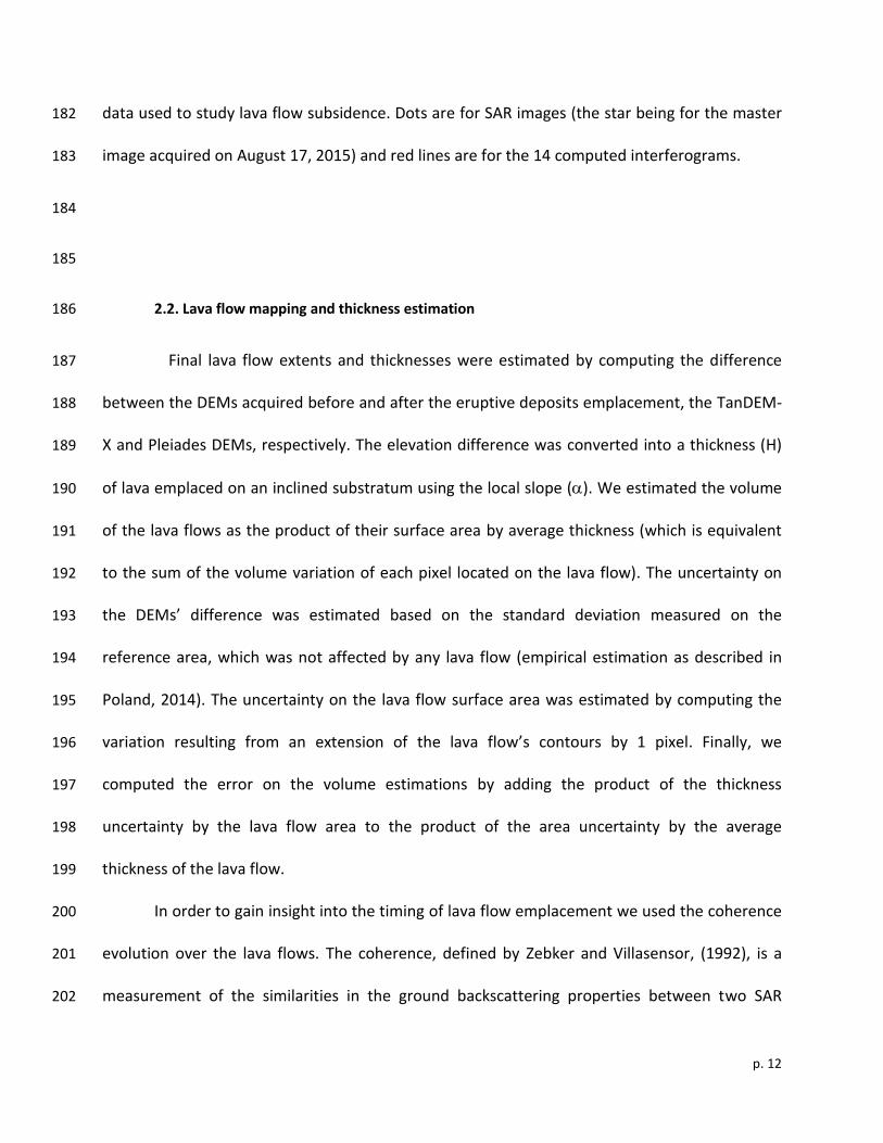
2.2. Lava flow mapping and thickness estimation 186

Final lava flow extents and thicknesses were estimated by computing the difference 187

between the DEMs acquired before and after the eruptive deposits emplacement, the TanDEM-188

X and Pleiades DEMs, respectively. The elevation difference was converted into a thickness (H) 189

of lava emplaced on an inclined substratum using the local slope (). We estimated the volume 190

of the lava flows as the product of their surface area by average thickness (which is equivalent 191

to the sum of the volume variation of each pixel located on the lava flow). The uncertainty on 192

the DEMs’ difference was estimated based on the standard deviation measured on the 193

reference area, which was not affected by any lava flow (empirical estimation as described in 194

Poland, 2014). The uncertainty on the lava flow surface area was estimated by computing the 195

variation resulting from an extension of the lava flow’s contours by 1 pixel. Finally, we 196

computed the error on the volume estimations by adding the product of the thickness 197

uncertainty by the lava flow area to the product of the area uncertainty by the average 198

thickness of the lava flow. 199

In order to gain insight into the timing of lava flow emplacement we used the coherence 200

evolution over the lava flows. The coherence, defined by Zebker and Villasensor, (1992), is a 201

measurement of the similarities in the ground backscattering properties between two SAR 202

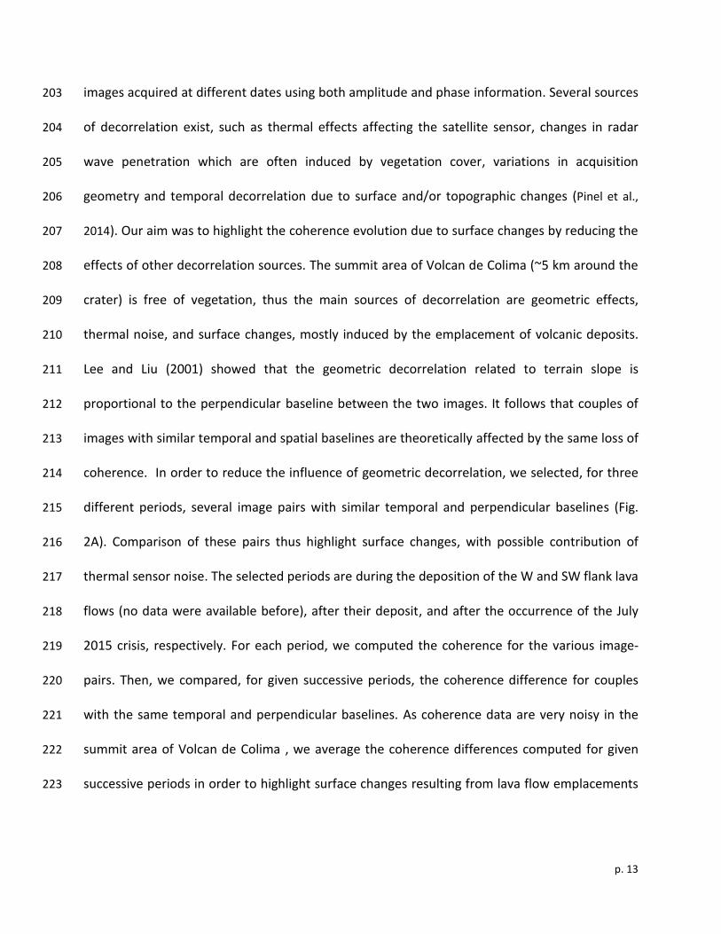
p. 13

images acquired at different dates using both amplitude and phase information. Several sources 203

of decorrelation exist, such as thermal effects affecting the satellite sensor, changes in radar 204

wave penetration which are often induced by vegetation cover, variations in acquisition 205

geometry and temporal decorrelation due to surface and/or topographic changes (Pinel et al., 206

2014). Our aim was to highlight the coherence evolution due to surface changes by reducing the 207

effects of other decorrelation sources. The summit area of Volcan de Colima (~5 km around the 208

crater) is free of vegetation, thus the main sources of decorrelation are geometric effects, 209

thermal noise, and surface changes, mostly induced by the emplacement of volcanic deposits. 210

Lee and Liu (2001) showed that the geometric decorrelation related to terrain slope is 211

proportional to the perpendicular baseline between the two images. It follows that couples of 212

images with similar temporal and spatial baselines are theoretically affected by the same loss of 213

coherence. In order to reduce the influence of geometric decorrelation, we selected, for three 214

different periods, several image pairs with similar temporal and perpendicular baselines (Fig. 215

2A). Comparison of these pairs thus highlight surface changes, with possible contribution of 216

thermal sensor noise. The selected periods are during the deposition of the W and SW flank lava 217

flows (no data were available before), after their deposit, and after the occurrence of the July 218

2015 crisis, respectively. For each period, we computed the coherence for the various image-219

pairs. Then, we compared, for given successive periods, the coherence difference for couples 220

with the same temporal and perpendicular baselines. As coherence data are very noisy in the 221

summit area of Volcan de Colima , we average the coherence differences computed for given 222

successive periods in order to highlight surface changes resulting from lava flow emplacements 223

p. 14

rather than noise induced by frequent ash emissions (Pinel et al., 2011) and thermal sensor 224

effects. 225

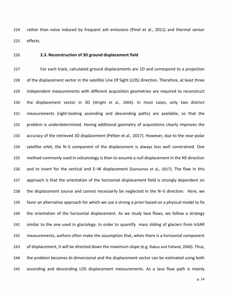
2.3. Reconstruction of 3D ground displacement field 226

For each track, calculated ground displacements are 1D and correspond to a projection 227

of the displacement vector in the satellite Line Of Sight (LOS) direction. Therefore, at least three 228

independent measurements with different acquisition geometries are required to reconstruct 229

the displacement vector in 3D (Wright et al., 2004). In most cases, only two distinct 230

measurements (right-looking ascending and descending paths) are available, so that the 231

problem is underdetermined. Having additional geometry of acquisitions clearly improves the 232

accuracy of the retrieved 3D displacement (Peltier et al., 2017). However, due to the near-polar 233

satellite orbit, the N‒S component of the displacement is always less well constrained. One 234

method commonly used in volcanology is then to assume a null displacement in the NS direction 235

and to invert for the vertical and E‒W displacement (Samsonov et al., 2017). The flaw in this 236

approach is that the orientation of the horizontal displacement field is strongly dependent on 237

the displacement source and cannot necessarily be neglected in the N‒S direction. Here, we 238

favor an alternative approach for which we use a strong a priori based on a physical model to fix 239

the orientation of the horizontal displacement. As we study lava flows, we follow a strategy 240

similar to the one used in glaciology. In order to quantify mass sliding of glaciers from InSAR 241

measurements, authors often make the assumption that, when there is a horizontal component 242

of displacement, it will be directed down the maximum slope (e.g. Rabus and Fatland, 2000). Thus, 243

the problem becomes bi-dimensional and the displacement vector can be estimated using both 244

ascending and descending LOS displacement measurements. As a lava flow path is mainly 245

p. 15

controlled by the topography (Felpeto et al., 2001; Mossoux et al., 2016), the same assumption can 246

be made for lava flows by considering that, if a bulk horizontal motion is observed, it should be 247

aligned with the direction of maximum slope. 248

249

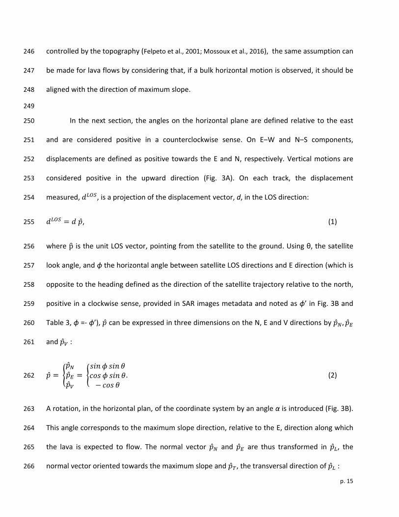
In the next section, the angles on the horizontal plane are defined relative to the east 250

and are considered positive in a counterclockwise sense. On E‒W and N‒S components, 251

displacements are defined as positive towards the E and N, respectively. Vertical motions are 252

considered positive in the upward direction (Fig. 3A). On each track, the displacement 253

measured, 𝑑𝐿𝑂𝑆, is a projection of the displacement vector, d, in the LOS direction: 254

𝑑𝐿𝑂𝑆 = 𝑑 �̂�, (1) 255

where p̂ is the unit LOS vector, pointing from the satellite to the ground. Using θ, the satellite 256

look angle, and ϕ the horizontal angle between satellite LOS directions and E direction (which is 257

opposite to the heading defined as the direction of the satellite trajectory relative to the north, 258

positive in a clockwise sense, provided in SAR images metadata and noted as ϕ’ in Fig. 3B and 259

Table 3, ϕ =- ϕ’), �̂� can be expressed in three dimensions on the N, E and V directions by �̂�𝑁 , �̂�𝐸 260

and �̂�𝑉 : 261

�̂� = {

�̂�𝑁

�̂�𝐸

�̂�𝑉

= {𝑠𝑖𝑛 𝜙 𝑠𝑖𝑛 𝜃𝑐𝑜𝑠 𝜙 𝑠𝑖𝑛 𝜃

− 𝑐𝑜𝑠 𝜃

. (2) 262

A rotation, in the horizontal plan, of the coordinate system by an angle α is introduced (Fig. 3B). 263

This angle corresponds to the maximum slope direction, relative to the E, direction along which 264

the lava is expected to flow. The normal vector �̂�𝑁 and �̂�𝐸 are thus transformed in �̂�𝐿, the 265

normal vector oriented towards the maximum slope and �̂�𝑇, the transversal direction of �̂�𝐿 : 266

p. 16

�̂� = {

�̂�𝑁

�̂�𝐸

�̂�𝑉

=> �̂� = {

�̂�𝐿

�̂�𝑇

�̂�𝑉

= {𝑐𝑜𝑠 𝜙 𝑠𝑖𝑛 𝜃 𝑐𝑜𝑠 𝛼 + 𝑠𝑖𝑛 𝜙 𝑠𝑖𝑛 𝜃 𝑠𝑖𝑛 𝛼𝑠𝑖𝑛 𝜙 𝑠𝑖𝑛 𝜃 𝑐𝑜𝑠 𝛼 − 𝑐𝑜𝑠 𝜙 𝑠𝑖𝑛 𝜃 𝑠𝑖𝑛 𝛼

− 𝑐𝑜𝑠 𝜃

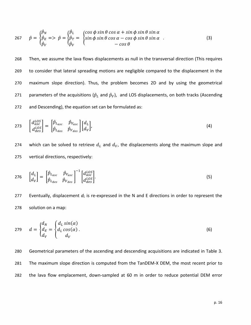
. (3) 267

Then, we assume the lava flows displacements as null in the transversal direction (This requires 268

to consider that lateral spreading motions are negligible compared to the displacement in the 269

maximum slope direction). Thus, the problem becomes 2D and by using the geometrical 270

parameters of the acquisitions (�̂�𝐿 and �̂�𝑉), and LOS displacements, on both tracks (Ascending 271

and Descending), the equation set can be formulated as: 272

[𝑑𝑎𝑠𝑐

𝐿𝑂𝑆

𝑑𝑑𝑒𝑠𝐿𝑂𝑆] = [

�̂�𝐿𝑎𝑠𝑐�̂�𝑉𝑎𝑠𝑐

�̂�𝐿𝑑𝑒𝑠�̂�𝑉𝑑𝑒𝑠

] [

𝑑𝐿

𝑑𝑉], (4) 273

which can be solved to retrieve 𝑑𝐿 and 𝑑𝑉, the displacements along the maximum slope and 274

vertical directions, respectively: 275

[𝑑𝐿

𝑑𝑉] = [

�̂�𝐿𝑎𝑠𝑐�̂�𝑉𝑎𝑠𝑐

�̂�𝐿𝑑𝑒𝑠�̂�𝑉𝑑𝑒𝑠

]

−1

[𝑑𝑎𝑠𝑐

𝐿𝑂𝑆

𝑑𝑑𝑒𝑠𝐿𝑂𝑆]. (5) 276

Eventually, displacement dL is re-expressed in the N and E directions in order to represent the 277

solution on a map: 278

𝑑 = {

𝑑𝑁

𝑑𝐸

𝑑𝑉

= {

𝑑𝐿 𝑠𝑖𝑛(𝛼)

𝑑𝐿 𝑐𝑜𝑠(𝛼) 𝑑𝑉

. (6) 279

Geometrical parameters of the ascending and descending acquisitions are indicated in Table 3. 280

The maximum slope direction is computed from the TanDEM-X DEM, the most recent prior to 281

the lava flow emplacement, down-sampled at 60 m in order to reduce potential DEM error 282

p. 17

effects. For each pixel covered by both tracks, we used Eq. 5‒6 with the local maximum slope 283

direction to obtain a map of vertical and horizontal displacements. 284

285

286

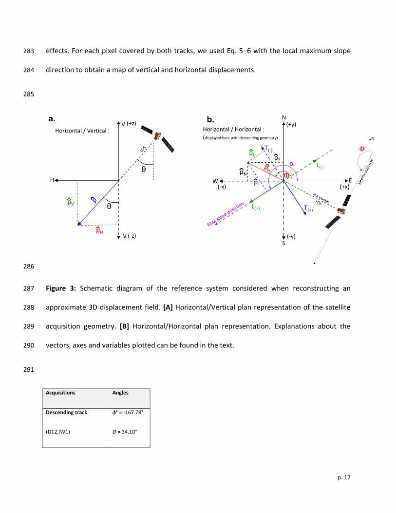
Figure 3: Schematic diagram of the reference system considered when reconstructing an 287

approximate 3D displacement field. [A] Horizontal/Vertical plan representation of the satellite 288

acquisition geometry. [B] Horizontal/Horizontal plan representation. Explanations about the 289

vectors, axes and variables plotted can be found in the text. 290

291

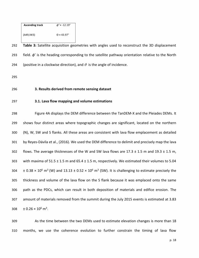
Acquisitions Angles

Descending track ϕ’ = -167.78°

(D12,IW1) Θ = 34.10°

p. 18

Ascending track ϕ’ = -12.19°

(A49,IW3) Θ = 43.97°

Table 3: Satellite acquisition geometries with angles used to reconstruct the 3D displacement 292

field. ϕ’ is the heading corresponding to the satellite pathway orientation relative to the North 293

(positive in a clockwise direction), and is the angle of incidence. 294

295

3. Results derived from remote sensing dataset 296

3.1. Lava flow mapping and volume estimations 297

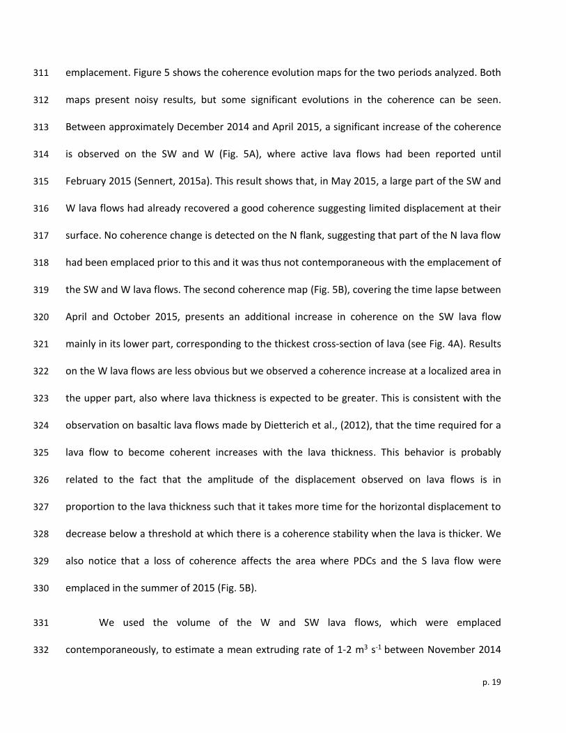
Figure 4A displays the DEM difference between the TanDEM-X and the Pleiades DEMs. It 298

shows four distinct areas where topographic changes are significant, located on the northern 299

(N), W, SW and S flanks. All these areas are consistent with lava flow emplacement as detailed 300

by Reyes-Dávila et al., (2016). We used the DEM difference to delimit and precisely map the lava 301

flows. The average thicknesses of the W and SW lava flows are 17.3 ± 1.5 m and 19.3 ± 1.5 m, 302

with maxima of 51.5 ± 1.5 m and 65.4 ± 1.5 m, respectively. We estimated their volumes to 5.04 303

± 0.38 × 106 m3 (W) and 13.13 ± 0.52 × 106 m3 (SW). It is challenging to estimate precisely the 304

thickness and volume of the lava flow on the S flank because it was emplaced onto the same 305

path as the PDCs, which can result in both deposition of materials and edifice erosion. The 306

amount of materials removed from the summit during the July 2015 events is estimated at 3.83 307

± 0.26 × 106 m3. 308

As the time between the two DEMs used to estimate elevation changes is more than 18 309

months, we use the coherence evolution to further constrain the timing of lava flow 310

p. 19

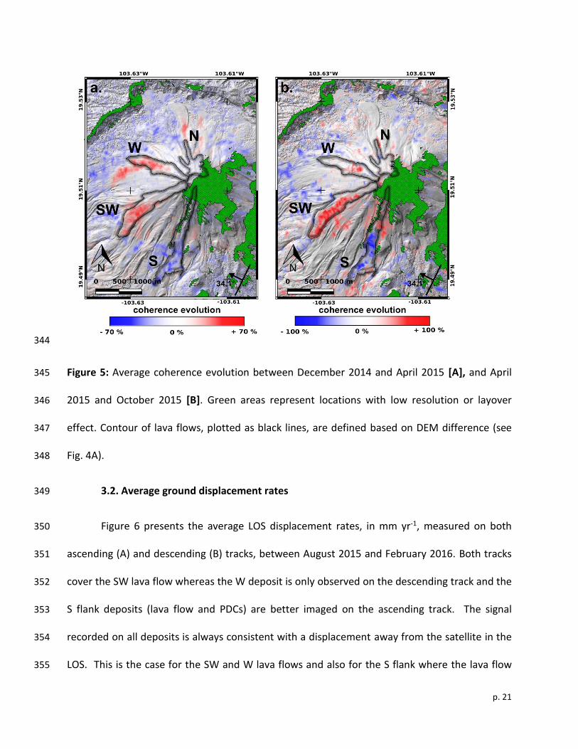
emplacement. Figure 5 shows the coherence evolution maps for the two periods analyzed. Both 311

maps present noisy results, but some significant evolutions in the coherence can be seen. 312

Between approximately December 2014 and April 2015, a significant increase of the coherence 313

is observed on the SW and W (Fig. 5A), where active lava flows had been reported until 314

February 2015 (Sennert, 2015a). This result shows that, in May 2015, a large part of the SW and 315

W lava flows had already recovered a good coherence suggesting limited displacement at their 316

surface. No coherence change is detected on the N flank, suggesting that part of the N lava flow 317

had been emplaced prior to this and it was thus not contemporaneous with the emplacement of 318

the SW and W lava flows. The second coherence map (Fig. 5B), covering the time lapse between 319

April and October 2015, presents an additional increase in coherence on the SW lava flow 320

mainly in its lower part, corresponding to the thickest cross-section of lava (see Fig. 4A). Results 321

on the W lava flows are less obvious but we observed a coherence increase at a localized area in 322

the upper part, also where lava thickness is expected to be greater. This is consistent with the 323

observation on basaltic lava flows made by Dietterich et al., (2012), that the time required for a 324

lava flow to become coherent increases with the lava thickness. This behavior is probably 325

related to the fact that the amplitude of the displacement observed on lava flows is in 326

proportion to the lava thickness such that it takes more time for the horizontal displacement to 327

decrease below a threshold at which there is a coherence stability when the lava is thicker. We 328

also notice that a loss of coherence affects the area where PDCs and the S lava flow were 329

emplaced in the summer of 2015 (Fig. 5B). 330

We used the volume of the W and SW lava flows, which were emplaced 331

contemporaneously, to estimate a mean extruding rate of 1-2 m3 s-1 between November 2014 332

p. 20

and February 2015. We have not taken into account the small volume (< 2 × 106 m3) of the N 333

lava flow on the coherence map, as its emplacement timing is not well constrained implying that 334

the estimated extrusion rate might be slightly underestimated. 335

336

337

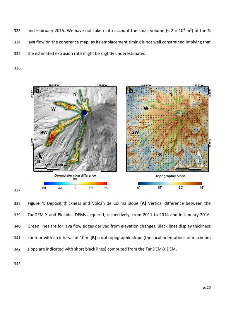
Figure 4: Deposit thickness and Volcán de Colima slope [A] Vertical difference between the 338

TanDEM-X and Pleiades DEMs acquired, respectively, from 2011 to 2014 and in January 2016. 339

Green lines are for lava flow edges derived from elevation changes. Black lines display thickness 340

contour with an interval of 10m. [B] Local topographic slope (the local orientations of maximum 341

slope are indicated with short black lines) computed from the TanDEM-X DEM. 342

343

p. 21

344

Figure 5: Average coherence evolution between December 2014 and April 2015 [A], and April 345

2015 and October 2015 [B]. Green areas represent locations with low resolution or layover 346

effect. Contour of lava flows, plotted as black lines, are defined based on DEM difference (see 347

Fig. 4A). 348

3.2. Average ground displacement rates 349

Figure 6 presents the average LOS displacement rates, in mm yr-1, measured on both 350

ascending (A) and descending (B) tracks, between August 2015 and February 2016. Both tracks 351

cover the SW lava flow whereas the W deposit is only observed on the descending track and the 352

S flank deposits (lava flow and PDCs) are better imaged on the ascending track. The signal 353

recorded on all deposits is always consistent with a displacement away from the satellite in the 354

LOS. This is the case for the SW and W lava flows and also for the S flank where the lava flow 355

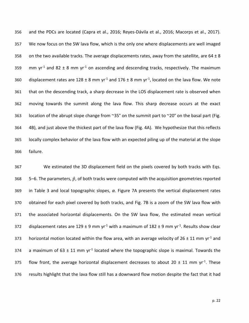
p. 22

and the PDCs are located (Capra et al., 2016; Reyes-Dávila et al., 2016; Macorps et al., 2017). 356

We now focus on the SW lava flow, which is the only one where displacements are well imaged 357

on the two available tracks. The average displacements rates, away from the satellite, are 64 ± 8 358

mm yr-1 and 82 ± 8 mm yr-1 on ascending and descending tracks, respectively. The maximum 359

displacement rates are 128 ± 8 mm yr-1 and 176 ± 8 mm yr-1, located on the lava flow. We note 360

that on the descending track, a sharp decrease in the LOS displacement rate is observed when 361

moving towards the summit along the lava flow. This sharp decrease occurs at the exact 362

location of the abrupt slope change from ~35° on the summit part to ~20° on the basal part (Fig. 363

4B), and just above the thickest part of the lava flow (Fig. 4A). We hypothesize that this reflects 364

locally complex behavior of the lava flow with an expected piling up of the material at the slope 365

failure. 366

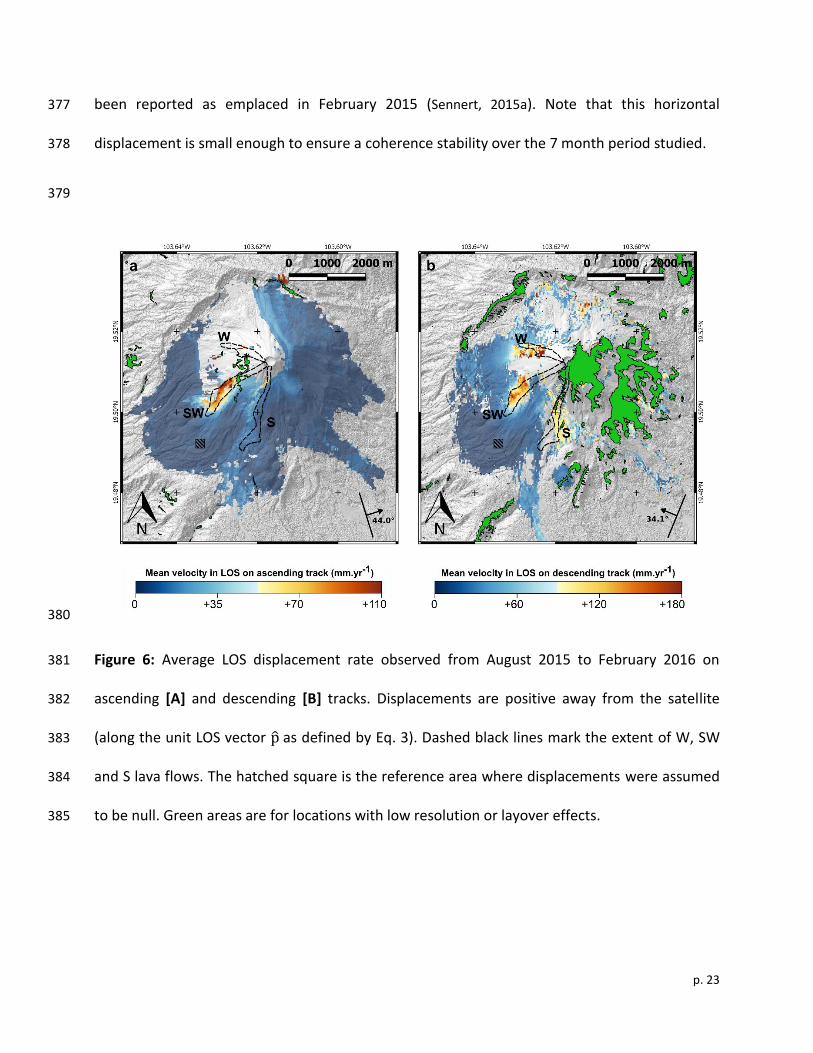
We estimated the 3D displacement field on the pixels covered by both tracks with Eqs. 367

5‒6. The parameters, �̂�, of both tracks were computed with the acquisition geometries reported 368

in Table 3 and local topographic slopes, α. Figure 7A presents the vertical displacement rates 369

obtained for each pixel covered by both tracks, and Fig. 7B is a zoom of the SW lava flow with 370

the associated horizontal displacements. On the SW lava flow, the estimated mean vertical 371

displacement rates are 129 ± 9 mm yr-1 with a maximum of 182 ± 9 mm yr-1. Results show clear 372

horizontal motion located within the flow area, with an average velocity of 26 ± 11 mm yr-1 and 373

a maximum of 63 ± 11 mm yr-1 located where the topographic slope is maximal. Towards the 374

flow front, the average horizontal displacement decreases to about 20 ± 11 mm yr-1. These 375

results highlight that the lava flow still has a downward flow motion despite the fact that it had 376

p. 23

been reported as emplaced in February 2015 (Sennert, 2015a). Note that this horizontal 377

displacement is small enough to ensure a coherence stability over the 7 month period studied. 378

379

380

Figure 6: Average LOS displacement rate observed from August 2015 to February 2016 on 381

ascending [A] and descending [B] tracks. Displacements are positive away from the satellite 382

(along the unit LOS vector p̂ as defined by Eq. 3). Dashed black lines mark the extent of W, SW 383

and S lava flows. The hatched square is the reference area where displacements were assumed 384

to be null. Green areas are for locations with low resolution or layover effects. 385

p. 24

386

Figure 7: 3D displacement field of the SW lava flow [A] Mean vertical displacement rate (from 387

August 2015 to February 2016). Positive values are for an upward displacement. Green areas 388

represent places affected by very low resolution or layover on both tracks. The hatched square 389

is the reference area where displacements are assumed to be null. The red rectangle shows the 390

extent of the zoom displayed in Fig.7B. [B] Zoom of the SW lava flow with horizontal motion 391

vectors. Circles represent the uncertainties on displacement vectors. Dashed black lines mark 392

the edges of lava flows derived from DEMs difference. Note that whereas the horizontal 393

displacements are negligible outside the lava flow, the vertical ones remain significant around 394

the lava flow due to loading effects. 395

396

p. 25

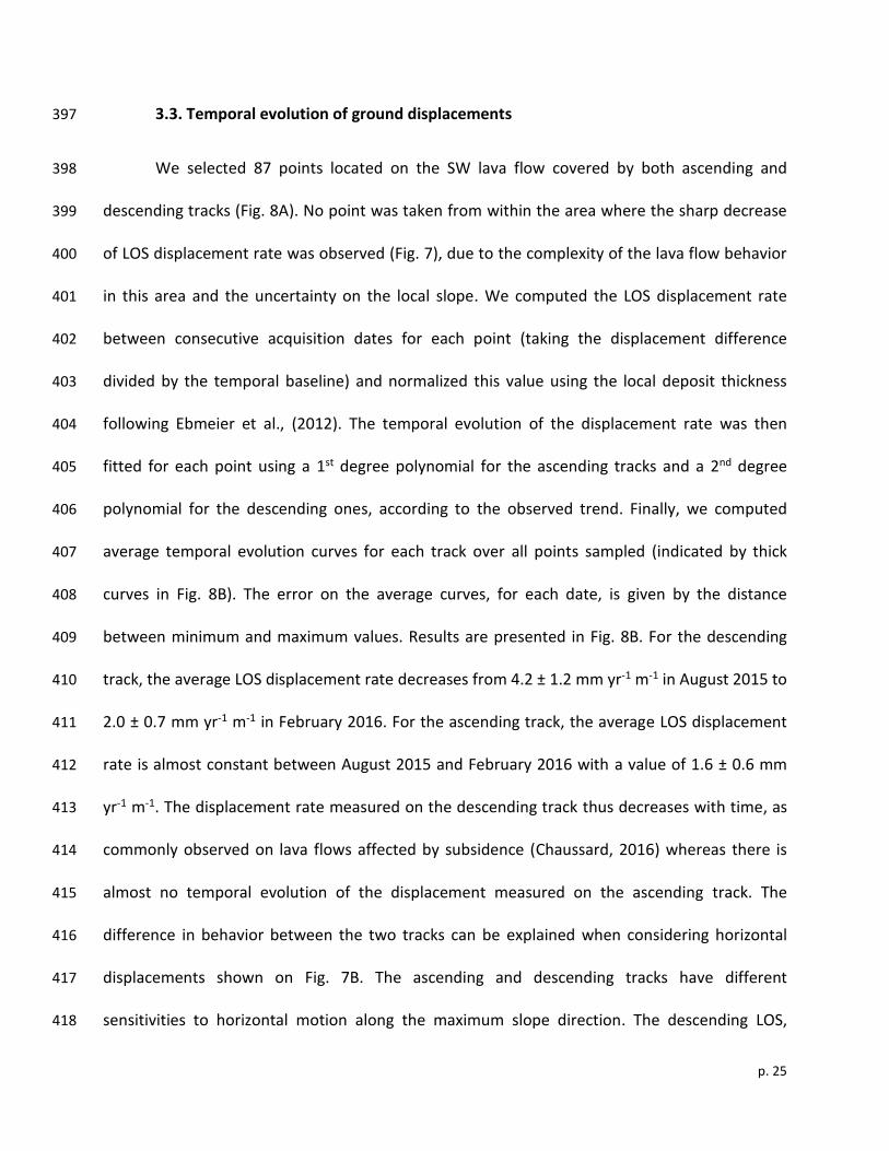
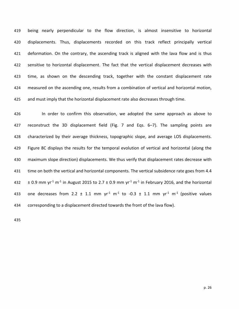
3.3. Temporal evolution of ground displacements 397

We selected 87 points located on the SW lava flow covered by both ascending and 398

descending tracks (Fig. 8A). No point was taken from within the area where the sharp decrease 399

of LOS displacement rate was observed (Fig. 7), due to the complexity of the lava flow behavior 400

in this area and the uncertainty on the local slope. We computed the LOS displacement rate 401

between consecutive acquisition dates for each point (taking the displacement difference 402

divided by the temporal baseline) and normalized this value using the local deposit thickness 403

following Ebmeier et al., (2012). The temporal evolution of the displacement rate was then 404

fitted for each point using a 1st degree polynomial for the ascending tracks and a 2nd degree 405

polynomial for the descending ones, according to the observed trend. Finally, we computed 406

average temporal evolution curves for each track over all points sampled (indicated by thick 407

curves in Fig. 8B). The error on the average curves, for each date, is given by the distance 408

between minimum and maximum values. Results are presented in Fig. 8B. For the descending 409

track, the average LOS displacement rate decreases from 4.2 ± 1.2 mm yr-1 m-1 in August 2015 to 410

2.0 ± 0.7 mm yr-1 m-1 in February 2016. For the ascending track, the average LOS displacement 411

rate is almost constant between August 2015 and February 2016 with a value of 1.6 ± 0.6 mm 412

yr-1 m-1. The displacement rate measured on the descending track thus decreases with time, as 413

commonly observed on lava flows affected by subsidence (Chaussard, 2016) whereas there is 414

almost no temporal evolution of the displacement measured on the ascending track. The 415

difference in behavior between the two tracks can be explained when considering horizontal 416

displacements shown on Fig. 7B. The ascending and descending tracks have different 417

sensitivities to horizontal motion along the maximum slope direction. The descending LOS, 418

p. 26

being nearly perpendicular to the flow direction, is almost insensitive to horizontal 419

displacements. Thus, displacements recorded on this track reflect principally vertical 420

deformation. On the contrary, the ascending track is aligned with the lava flow and is thus 421

sensitive to horizontal displacement. The fact that the vertical displacement decreases with 422

time, as shown on the descending track, together with the constant displacement rate 423

measured on the ascending one, results from a combination of vertical and horizontal motion, 424

and must imply that the horizontal displacement rate also decreases through time. 425

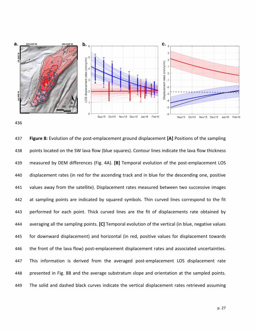
In order to confirm this observation, we adopted the same approach as above to 426

reconstruct the 3D displacement field (Fig. 7 and Eqs. 6‒7). The sampling points are 427

characterized by their average thickness, topographic slope, and average LOS displacements. 428

Figure 8C displays the results for the temporal evolution of vertical and horizontal (along the 429

maximum slope direction) displacements. We thus verify that displacement rates decrease with 430

time on both the vertical and horizontal components. The vertical subsidence rate goes from 4.4 431

± 0.9 mm yr-1 m-1 in August 2015 to 2.7 ± 0.9 mm yr-1 m-1 in February 2016, and the horizontal 432

one decreases from 2.2 ± 1.1 mm yr-1 m-1 to -0.3 ± 1.1 mm yr-1 m-1 (positive values 433

corresponding to a displacement directed towards the front of the lava flow). 434

435

p. 27

436

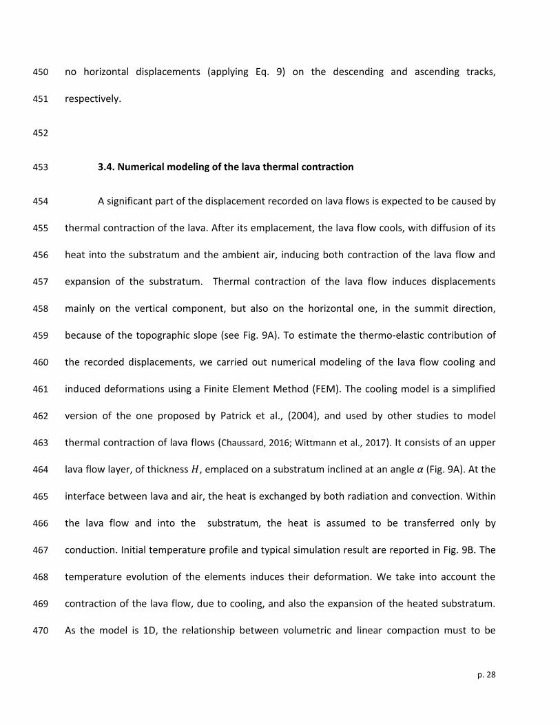
Figure 8: Evolution of the post-emplacement ground displacement [A] Positions of the sampling 437

points located on the SW lava flow (blue squares). Contour lines indicate the lava flow thickness 438

measured by DEM differences (Fig. 4A). [B] Temporal evolution of the post-emplacement LOS 439

displacement rates (in red for the ascending track and in blue for the descending one, positive 440

values away from the satellite). Displacement rates measured between two successive images 441

at sampling points are indicated by squared symbols. Thin curved lines correspond to the fit 442

performed for each point. Thick curved lines are the fit of displacements rate obtained by 443

averaging all the sampling points. [C] Temporal evolution of the vertical (in blue, negative values 444

for downward displacement) and horizontal (in red, positive values for displacement towards 445

the front of the lava flow) post-emplacement displacement rates and associated uncertainties. 446

This information is derived from the averaged post-emplacement LOS displacement rate 447

presented in Fig. 8B and the average substratum slope and orientation at the sampled points. 448

The solid and dashed black curves indicate the vertical displacement rates retrieved assuming 449

p. 28

no horizontal displacements (applying Eq. 9) on the descending and ascending tracks, 450

respectively. 451

452

3.4. Numerical modeling of the lava thermal contraction 453

A significant part of the displacement recorded on lava flows is expected to be caused by 454

thermal contraction of the lava. After its emplacement, the lava flow cools, with diffusion of its 455

heat into the substratum and the ambient air, inducing both contraction of the lava flow and 456

expansion of the substratum. Thermal contraction of the lava flow induces displacements 457

mainly on the vertical component, but also on the horizontal one, in the summit direction, 458

because of the topographic slope (see Fig. 9A). To estimate the thermo-elastic contribution of 459

the recorded displacements, we carried out numerical modeling of the lava flow cooling and 460

induced deformations using a Finite Element Method (FEM). The cooling model is a simplified 461

version of the one proposed by Patrick et al., (2004), and used by other studies to model 462

thermal contraction of lava flows (Chaussard, 2016; Wittmann et al., 2017). It consists of an upper 463

lava flow layer, of thickness 𝐻, emplaced on a substratum inclined at an angle α (Fig. 9A). At the 464

interface between lava and air, the heat is exchanged by both radiation and convection. Within 465

the lava flow and into the substratum, the heat is assumed to be transferred only by 466

conduction. Initial temperature profile and typical simulation result are reported in Fig. 9B. The 467

temperature evolution of the elements induces their deformation. We take into account the 468

contraction of the lava flow, due to cooling, and also the expansion of the heated substratum. 469

As the model is 1D, the relationship between volumetric and linear compaction must to be 470

p. 29

taken into account by involving the Poisson coefficient (Chaussard, 2016; Wittmann et al., 471

2017). Key points of the FEM implementation are given in the Supplementary Material SIA. 472

The morphology of the SW lava flow, is characterized by its short length and steep 473

edges, and is similar to flows reported on Merapi volcano (Indonesia) by Voight et al. (2000), 474

where lava tongues are fed by lava dome material extruded on the flank. We thus assume that 475

the materials emplaced in such flows has the same composition and properties as the dome 476

itself. This is confirmed by lava blocks collected on similar active lava flows, at Volcán de Colima 477

(Savov et al., 2008). The collected samples present low porosity probably due to degassing during 478

the slow ascent of the emplaced material through the conduit (Lavallée et al., 2012; Cassidy et 479

al., 2015). During its ascent and evolution inside the dome itself, the magma cools and 480

crystallizes as highlighted by the high SiO2 composition of glass in the dome clasts collected at 481

Volcán de Colima (Cassidy et al., 2015). As degassing and crystallization is already at an advanced 482

stage before lava flow emplacement, the vesiculation and latent heat effects during the cooling 483

of the lava flow are neglected in this study. 484

We assumed the lava flow and substratum to be of the same composition with their 485

conductivities, heat capacities and densities being only functions of the temperature. We 486

adopted the same approach as Patrick et al. (2004) to estimate the temperature dependence on 487

the thermal conductivity (k) for andesitic lavas. A fit of the conductivity measured on Mt Hood 488

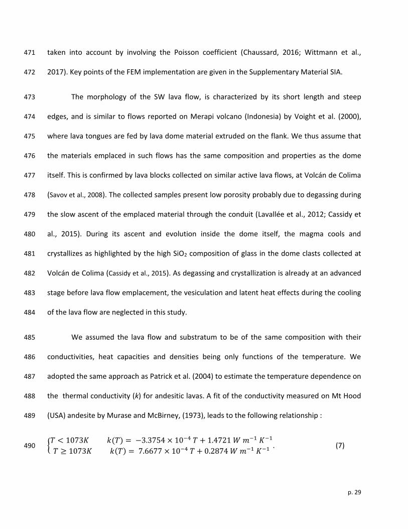
(USA) andesite by Murase and McBirney, (1973), leads to the following relationship : 489

{𝑇 < 1073𝐾 𝑘(𝑇) = −3.3754 × 10−4 𝑇 + 1.4721 𝑊 𝑚−1 𝐾−1

𝑇 ≥ 1073𝐾 𝑘(𝑇) = 7.6677 × 10−4 𝑇 + 0.2874 𝑊 𝑚−1 𝐾−1 . (7) 490

p. 30

The temperature dependence on the lava heat capacity is implemented in the same way as for 491

other lava flow cooling models (Patrick et al., 2004; Chaussard, 2016). Finally, the local density 492

evolution is computed based on the lava thermal expansion coefficient, β, as 493

𝜌(𝑇) = 𝜌𝑟𝑒𝑓 (1 + 𝛽 (𝑇 − 𝑇𝑟𝑒𝑓)). (8) 494

The thermal expansion coefficient is a key parameter that controls the lava flow thermal 495

contraction rate. Its values depend on several properties of the rock, such as temperature, crack 496

content, porosity, composition and history (Richter and Simmons, 1974; Bauer and Handin, 1983). As 497

no in situ measurements of the emplaced material are available, we used two end members 498

values from the literature (Murase and McBirney, 1973; Bauer and Handin, 1983; Mallela et al., 2005). 499

The lowest value is taken at β=1.0 × 10-5 K-1, and the maximum at β=3.5 × 10-5 K-1. The physical 500

parameters considered in the model are summarized in Table 4. The starting date of the 501

simulation (to) was chosen to be the middle of the deposition period between the time when 502

the lava flow started and the time when it was reported to be emplaced (after the supply rate 503

had ceased). This parameter cannot be more precisely estimated here, but its influence on the 504

predicted displacement rates decreases as time increases from to. As the InSAR time series 505

starts several months after the emplacement time, the uncertainty on this initial time has a 506

limited impact on the results of the modeled displacement velocity (less than ±5% here if the 507

starting date is moved by one month before or after the selected date used here). 508

Results of the numerical modeling, on the time lapse analyzed by the InSAR time series, 509

illustrate that thermal compaction of the lava flow produces displacement in both vertical and 510

horizontal directions (Fig. 10A). Not surprisingly, the estimated displacement rate, produced by 511

p. 31

thermo-elastic contraction, is strongly affected by the value of the thermal expansion 512

coefficient. With the maximum value, β=3.5 × 10-5 K-1, the predicted vertical displacement rate, 513

in the downward direction, is 134.2 mm yr-1 in August 2015, and decreases to 98.4 mm yr-1 in 514

February 2016. The associated horizontal displacement rates at these dates are 44.8 mm yr-1 515

and 32.9 mm yr-1 in the summit direction, respectively (Fig. 10A). When the thermal expansion 516

coefficient is β=1.0 × 10-5 K-1, the vertical subsidence rate decreases from 38.0 mm yr-1 to 28.0 517

mm yr-1 between August 2015 and February 2016. The corresponding horizontal rates are 12.7 518

mm yr-1 and 9.3 mm yr-1, respectively, towards the summit. 519

520

521

Figure 9: Lava flow cooling and contraction using numerical modelling [A] Conceptual model 522

used for thermal contraction. The solid blue vector indicates the expected surface displacement 523

associated with thermo-elastic compaction. The dashed blue vectors represent its projection on 524

the vertical and horizontal directions. The green arrow corresponds to the 1D direction 525

p. 32

considered in the numerical model and to the section represented in Fig. 9B. [B] Vertical 526

distribution of the temperature at initial conditions (red curve), and after 2 years of cooling 527

(blue curve). 528

529

p. 33

530

531

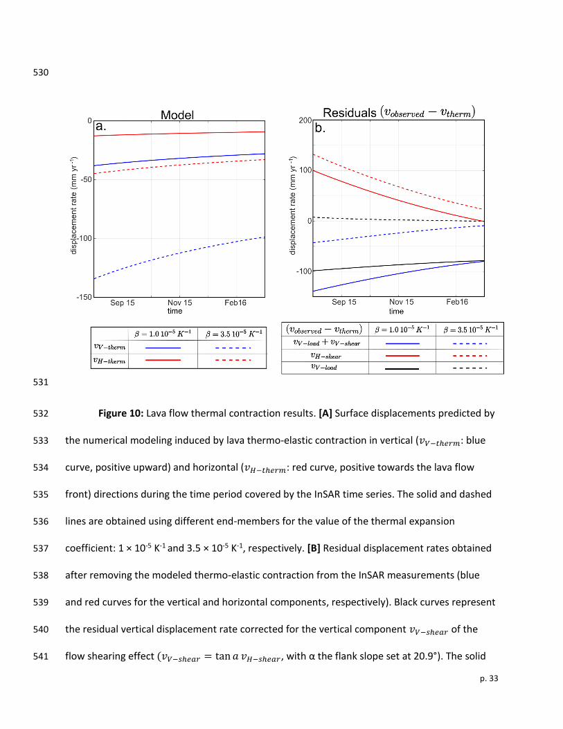
Figure 10: Lava flow thermal contraction results. [A] Surface displacements predicted by 532

the numerical modeling induced by lava thermo-elastic contraction in vertical (𝑣𝑉−𝑡ℎ𝑒𝑟𝑚: blue 533

curve, positive upward) and horizontal (𝑣𝐻−𝑡ℎ𝑒𝑟𝑚: red curve, positive towards the lava flow 534

front) directions during the time period covered by the InSAR time series. The solid and dashed 535

lines are obtained using different end-members for the value of the thermal expansion 536

coefficient: 1 × 10-5 K-1 and 3.5 × 10-5 K-1, respectively. [B] Residual displacement rates obtained 537

after removing the modeled thermo-elastic contraction from the InSAR measurements (blue 538

and red curves for the vertical and horizontal components, respectively). Black curves represent 539

the residual vertical displacement rate corrected for the vertical component 𝑣𝑉−𝑠ℎ𝑒𝑎𝑟 of the 540

flow shearing effect (𝑣𝑉−𝑠ℎ𝑒𝑎𝑟 = tan 𝑎 𝑣𝐻−𝑠ℎ𝑒𝑎𝑟, with α the flank slope set at 20.9°). The solid 541

p. 34

and dashed lines, respectively, are obtained using different end-members for the value of the 542

thermal expansion coefficient: 1 × 10-5 K-1 and 3.5 × 10-5 K-1, respectively. 543

544

Parameter Model input (Units) Reference

Geometrical parameters

Lava flow thickness : H 40.6 m This study

Substratum thickness 100 m -

Substratum tilt 20.9° This study

Physical parameters

Air dynamic viscosity : ηa 1.725 × 10-5 Pa s -

Air heat capacity : Cpa 1006 J kg-1 K-1 -

Air temperature : Ta 20 °C -

Air thermal expansion coef. : βa 3.69 × 10-3 K-1 -

Initial lava flow temperature : Tini 800 °C -

Initial substratum temperature : Tsub 20 °C -

Lava flow emissivity : ε 0.925 (Salisbury and D’Aria, 1994)

Reference lava density at Tref : ρref 2630 kg m-3 (Luhr, 2002)

Reference temperature: Tref 20°C (Luhr, 2002)

Simulation start date 01/01/2015 -

Thermal expansion coefficient : β 1 × 10-5 K-1 or 3.5 × 10-5 K-1 (Bauer and Handin, 1983; Mallela et al., 2005; Murase and McBirney, 1973)

Numerical parameters

Polynomial degree of elements 1 -

Number of elements into the flow 100 -

Number of elements into the substratum 200 -

Stability coefficient 0.01 -

545

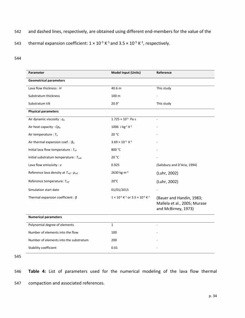
Table 4: List of parameters used for the numerical modeling of the lava flow thermal 546

compaction and associated references. 547

p. 35

548

4. Discussion 549

4.1 The 2014-2015 effusive activity of Volcàn de Colima 550

Using the DEM difference (Fig. 4A) together with the temporal constrain provided by 551

coherence evolution, we identified at least 3 massive lava flows emplaced between November 552

2014 and July 2015. Two of them (W and S‒W) results from the overflow of the dome near the 553

end of 2014. The third one (S) occurred after the July 2015 explosion. Each lava flow is thick and 554

presents sharp edges, which suggests here the small influence of spreading and breakout effects 555

as sometimes described in the literature (Tuffen et al., 2013). Both S‒W and S lava flows show 556

an increased in their thickness close to their front (Fig 4A). This increases might be associated 557

with the sharp decrease of the topographic slope (from ~25° to 15°~, Fig. 4B). On the contrary, 558

the W lava flow does not present the same increased in its thickness near its front, probably 559

related to the absence of significant slope change along the lava flow. 560

The extruding rate we estimate around 1-2 m3 s-1 between November 2014 and 561

February 2015 is 100 to 1000 times higher than the extruding rates derived in 2010‒2011 from 562

the seismic signature of rockfalls (Mueller et al., 2013), and 15 to 30 times larger than published 563

estimations for the long term extrusion rate (Luhr and Carmichael, 1980; Luhr and Prestegaard, 564

1988). It highlights the temporal variations in the extrusion rate as already previously evidenced 565

(Mueller et al., 2013). This larger value might also evidence an increase in the volcano activity 566

preceding the large July 2015 eruptive event. 567

p. 36

4.2. Use of physical a priori to retrieve the 3D displacement field from InSAR 568

measurements: 569

Most InSAR studies dealing with lava flows deformation consider the LOS displacement 570

as the projection of a vertical motion along the LOS using the following equation (e.g. Wittmann 571

et al., 2017): 572

𝑑𝑉 = −𝑑𝐿𝑂𝑆

𝑐𝑜𝑠 (𝜃) (9) 573

In order to test the validity of this assumption, we computed the vertical displacement 574

rate using Eq. 9 for both ascending and descending tracks. As the horizontal viewing angle, on 575

the descending track, is almost perpendicular to the direction of the flow, the results obtained 576

are similar to the ones derived with our approach based on the physical a priori that the 577

horizontal displacement is directed along the maximum slope. This is clearly not the case on the 578

ascending track for which the horizontal motion cannot be neglected except at the end of the 579

studied period (Fig. 8C). However, after December 2015, horizontal motion becomes negligible 580

and LOS displacements for both tracks can be used alone to correctly estimate vertical 581

displacements. To summarize, Eq. 9 can only be applied when the LOS is perpendicular to the 582

flow direction (that is to say the horizontal projection of the satellite pathway is parallel to the 583

flow direction), or when horizontal motion is negligible. 584

The method we propose to reconstruct the 3D displacement field has the advantage of 585

relying on a physical a priori. We assume that the horizontal motion over the lava flow is 586

directed along the maximum slope direction. The use of this a priori is not necessary when 587

several geometries of acquisition from different satellites are available (Wright et al., 2004, 588

p. 37

Peltier et al., 2017). As in most studies, in our case only two tracks from the same satellite, the 589

ascending and descending ones, are available, but contrary to what is commonly done (e.g. 590

Samsonov et al., 2017) we do not consider the north-south displacement as null. Instead, we 591

consider that the direction of the horizontal motion is mainly controlled by the local 592

topography. This method can also be applied to studies dealing with other types of deformation 593

sources observed on volcanoes, such as reservoir pressurization or dike propagation. The 594

displacements associated with such sources are usually well predicted by simple analytical 595

models provided the sources are deep enough to preclude any strong influence of the 596

topography (e.g. Mogi, 1958 and Okada, 1985). By defining a given central pressurization point or 597

a given dislocation line, it is possible to predict the direction of the expected horizontal 598

displacement. Thus, our approach could potentially be used to reconstruct the 3D deformation 599

field on volcanoes, by introducing an a priori with respect to the horizontal displacement 600

direction, for both ascending and descending tracks of the same satellite. 601

602

4.3. Origin of deformation: magma downward flow contribution in addition to thermal 603

compaction and loading. 604

The vertical and horizontal displacements measured in Fig. 7‒8 have different causes 605

related to the deposit of a new lava flow: substratum deformation induced by a loading effect 606

(viscoelastic and poroelastic relaxations), thermal contractions, and possibly displacements 607

resulting from the ongoing flow, or shearing, of the lava on the flank (Fig. 11A). The two latter 608

effects are limited to the lava flow itself, whereas the loading effect extends beyond the lava 609

p. 38

flow contour line. In the following section, we investigate the various potential causes of the 610

observed displacements in order to discriminate the relative importance of each effect. 611

When a flow is emplaced, it produces ground loading and induces viscoelastic and/or 612

poroelastic relaxation of the substratum and associated displacement in the vertical direction 613

(Briole et al., 1997; Lu et al., 2005). Poroelastic displacement can reach several centimeters but 614

only during the few days following lava flow emplacement (Lu et al., 2005). As the InSAR time 615

series starts a few months after the emplacement, poroelastic effects on the displacement rate 616

should be minimal. The viscous relaxation of the substratum is a slower process, and is expected 617

to be the main cause of the vertical subsidence observed around the flow (Fig. 7). Viscoelastic 618

deformation can be inferred from the load, which is directly proportional to the lava thickness, 619

although the estimate is strongly dependent on the substratum rheology profile. Two end 620

members are generally considered. The first end-member considers the substratum as an upper 621

finite viscoelastic layer of given thickness lying on a rigid material. The loading stress is then 622

assumed as constant within the upper layer (Briole et al., 1997). The second end-member 623

considers an infinite elastic half space, where the loading stress decreases with depth (Watanabe 624

et al., 2002). The amount and temporal evolution of viscoelastic displacement is strongly affected 625

by these assumptions. For example, after 1 year with the same load and with the same 626

substratum mechanical properties, the first assumption yields a displacement in the order of 627

centimeters, whereas the second one predicts deformation of the order of millimeters. A good 628

knowledge of the substratum structure and mechanical properties is required in order to make 629

a reliable estimate of the viscoelastic deformation. 630

p. 39

The displacement field induced by thermal compaction has been modeled in section 3.4. 631

Its amplitude is dependent on the poorly constrained thermal expansion coefficient but the 632

modeling results can be used to discuss the relative influence of this process. Figure 10B 633

displays the residuals obtained by removing our modeled thermo-elastic displacement from the 634

observed displacement rate (red and blue curves on Fig. 10B). The residual horizontal motion 635

can mostly be attributed to flow motion or lava flow shearing, depending on the amount of 636

friction at the lava flow/substratum interface. This is confirmed by the fact that horizontal 637

displacements recorded around the lava flow are very weak, indicating negligible horizontal 638

motion of the substratum. As sliding motion also produces vertical displacement, we estimated 639

and corrected the vertical displacement for this effect considering the volcano slope (see solid 640

and dashed black lines in Fig. 10B). With the largest thermal expansion coefficient (β=3.5 × 10-5 641

K-1), the residual vertical displacement is mostly explained by flow motion. That would imply 642

negligible viscoelastic deformation and would be in contradiction with the displacement 643

recorded on the substratum around the flow. Thus, the thermal contraction coefficient must be 644

lower than β=3.5 × 10-5 K-1. This is also supported by laboratory observations showing that the 645

thermal expansion coefficient decreased with the presence of cracks (Richter and Simmons, 1974). 646

Analysis of samples coming from the dome at Volcàn de Colima shows that a decrease in 647

temperature, or an increase in the strain rate, promotes the formation of cracks (Lavallée et al., 648

2012). The better agreement of the results with a low thermal expansion tends to indicate the 649

presence of cracks and fractures within the emplaced material. With the lowest thermal 650

expansion coefficient (β=1 × 10-5 K-1), the amplitude of the displacement induced by thermal 651

contraction is smaller. It follows that residual displacements are larger on the vertical 652

p. 40

component (where thermal compaction induces a downward displacement) and smaller on the 653

horizontal one (where thermal compaction induces an uphill displacement). Using a thermal 654

expansion coefficient β=1 × 10-5 K-1, the residual vertical displacement corrected for magma 655

flow effects decreases from 100.7 mm yr-1 to 79.4 mm yr-1 (plain black curve in Fig. 10B), which 656

is much more consistent with the average vertical displacements recorded around the lava flow 657

(Fig. 7). This residual value is expected to result from the viscoelastic compaction alone, acting 658

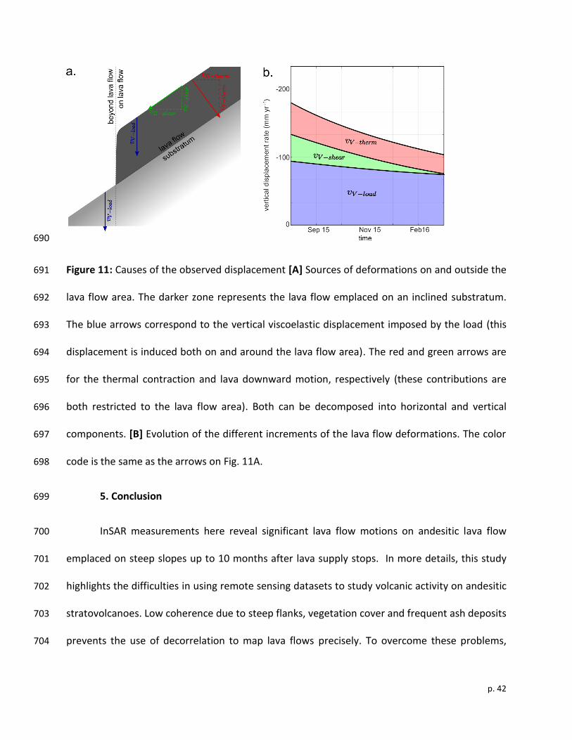
not only on the lava flow itself but also around it. Based on these estimates, the viscoelastic 659

compaction, the thermal contraction and the effect of downward lava flow would account for 660

about 50%, 25% and 25%, respectively, of the observed vertical displacement 8 months after 661

the magma flow emplacement (Fig. 11B). The amount of horizontal displacement produced by 662

lava downward flow (solid red curve on Fig. 10B) seems to decrease relatively rapidly with time 663

and tends towards zero at the end of the studied period. At this time, 75% of the observed 664

displacement can be explained by viscoelastic compaction, and 25% by thermal contraction of 665

the lava (Fig. 11B). 666

Lava flow motion had been evidenced several months after emplacement for rhyolitic 667

obsidian flow at Cordon Caulle volcano, Chile by field observations (Tuffen et al., 2013 ) but to 668

our knowledge such a downward flow displacement has never been isolated from InSAR 669

measurements before. The fact that it can be observed 8 months after the flow emplacement is 670

probably related to the high viscosity of this andesitic lava flow and the steepness of the slope 671

on the edifice flanks, two uncommon characteristics with regard to previous studies (see Table 672

1). This horizontal displacement can be used to calculate a rough estimate of the lava bulk 673

viscosity 𝜂. By considering that horizontal displacements result from the shearing of the lava 674

p. 41

flow (i.e. no slip at the lava/substratum interface) characterized by a Newtonian rheology, the 675

viscosity can be estimated with: 676

𝜂 = 𝜌 𝑔 𝐻2 sin 𝛼 cos 𝛼

2 𝑣ℎ, (10) 677

where 𝜌 = 2600 kg m-3, the lava bulk density, g, the gravitational acceleration, 𝐻 = 40.6m, the 678

lava flow thickness, 𝛼 = 20.9°, the volcano slope, and 𝑣ℎ, the horizontal surface displacement. 679

Equation 19 estimates the lava flow bulk viscosity at around 1015 Pa s in August 2015, at the 680

beginning of the studied period, and reaching a value of 1017 Pa s at the end of this period. The 681

assumption of a Newtonian behavior is not really expected to be verified for a highly crystalized 682

lava (Lavallée et al., 2007) and the temporal evolution of the viscosity we derived cannot be 683

explained by an Arrhenius law given the modeled variation in temperature. However, our 684

estimations both in terms of order of magnitude and temporal evolution are in relative good 685

agreement with the prediction from a general non-Arrhenius law for lava dome materials. In 686

particular, our estimations are consistent with the law linking the apparent viscosity of the 687

emplaced material and the shear rate derived by Lavallée et al., (2007) for moderate strain 688

rates (larger than the ones we measure) on dome material from Colima Volcano. 689

p. 42

690

Figure 11: Causes of the observed displacement [A] Sources of deformations on and outside the 691

lava flow area. The darker zone represents the lava flow emplaced on an inclined substratum. 692

The blue arrows correspond to the vertical viscoelastic displacement imposed by the load (this 693

displacement is induced both on and around the lava flow area). The red and green arrows are 694

for the thermal contraction and lava downward motion, respectively (these contributions are 695

both restricted to the lava flow area). Both can be decomposed into horizontal and vertical 696

components. [B] Evolution of the different increments of the lava flow deformations. The color 697

code is the same as the arrows on Fig. 11A. 698

5. Conclusion 699

InSAR measurements here reveal significant lava flow motions on andesitic lava flow 700

emplaced on steep slopes up to 10 months after lava supply stops. In more details, this study 701

highlights the difficulties in using remote sensing datasets to study volcanic activity on andesitic 702

stratovolcanoes. Low coherence due to steep flanks, vegetation cover and frequent ash deposits 703

prevents the use of decorrelation to map lava flows precisely. To overcome these problems, 704

p. 43

mapping can be performed using DEMs, with the additional advantage of being able to quantify 705

the volume of lava emplaced and to derive the associated eruption rate. At Volcàn de Colima, 706

we estimated a mean extrusion rate of around 1‒2 m3 s-1 over a 4 month period (November 707

2014 to February 2015). In order to maximize on the coherence, we use an alternative 708

approach to the classical one used on shield volcanoes, which is based on averaging the 709

difference between coherence maps characterized by similar spatio-temporal baselines in order 710

to highlight the timing of new deposits. We also propose an approach to reconstruct the 3D 711

displacement field of lava flows, from 2 viewing angles, using a physical assumption on the 712

horizontal motion direction, here considered to be controlled by the local topography. The 3D 713

displacement field retrieved at Volcán de Colima from InSAR time series inversions shows that 714

horizontal displacements are still significant on the SW lava flow a few months after lava 715

emplacement despite its apparent inactivity. Such behavior might be common on highly viscous 716

lava flows emplaced on steep slopes. Analysis of the observed displacements through numerical 717

modeling of the thermal compaction indicates that thermal contraction, viscoelastic loading, 718

and flow motion all play a significant role in the measured displacement field and brings 719

quantitative constrains on both the effective lava viscosity and its thermal expansion coefficient. 720

Acknowledgement: 721

This study was supported by CNES through the TOSCA project MerapiSAR. Pleiades images were 722

available through an ISIS project. SAR images were provided by ESA and downloaded from the 723

CNES operating platform at https://peps.cnes.fr/rocket/#/home. TanDEM-X DEM was provided 724

by the German Space Agency through proposal DEM_GEOL1315 (©DLR 2015). This manuscript 725

benefited greatly from the constructive reviews and comments of two anonymous reviewers. 726

Authors declare no conflict of interest. 727

References: 728

p. 44

Amelung, F., Day, S., 2002. InSAR observations of the 1995 Fogo, Cape Verde, eruption: Implications for 729 the effects of collapse events upon island volcanoes. Geophys. Res. Lett. 29, 47-1-47–4. 730

Arnold, D.W.D., Biggs, J., Anderson, K., Vallejo Vargas, S., Wadge, G., Ebmeier, S.K., Naranjo, M.F., 731 Mothes, P., 2017. Decaying Lava Extrusion Rate at El Reventador Volcano, Ecuador, Measured 732 Using High‐Resolution Satellite Radar. J. Geophys. Res. Solid Earth. 733

Bato, M.G., Froger, J.L., Harris, A.J.L., Villeneuve, N., 2016. Monitoring an effusive eruption at Piton de la 734 Fournaise using radar and thermal infrared remote sensing data: insights into the October 2010 735 eruption and its lava flows. Geol. Soc. Lond. Spec. Publ. 426, 533–552. 736 https://doi.org/10.1144/SP426.30 737

Bauer, S.J., Handin, J., 1983. Thermal expansion and cracking of three confined water-saturated igneous 738 rocks to 800°C. Rock Mech. Rock Eng. 16, 181–198. https://doi.org/10.1007/BF01033279 739

Briole, P., Massonnet, D., Delacourt, C., 1997. Post-eruptive deformation associated with the 1986–87 740 and 1989 lava flows of Etna detected by radar interferometry. Geophys. Res. Lett. 24, 37–40. 741 https://doi.org/10.1029/96GL03705 742

Broxton, M.J., Edwards, L.J., 2008. The Ames Stereo Pipeline: Automated 3D surface reconstruction from 743 orbital imagery, in: Lunar and Planetary Science Conference. p. 2419. 744

Capra, L., Macías, J.L., Cortés, A., Dávila, N., Saucedo, R., Osorio-Ocampo, S., Arce, J.L., Gavilanes-Ruiz, 745 J.C., Corona-Chávez, P., García-Sánchez, L., Sosa-Ceballos, G., Vázquez, R., 2016. Preliminary 746 report on the July 10–11, 2015 eruption at Volcán de Colima: Pyroclastic density currents with 747 exceptional runouts and volume. J. Volcanol. Geotherm. Res. 310, 39–49. 748 https://doi.org/10.1016/j.jvolgeores.2015.11.022 749

Cassidy, M., Cole, Paul.D., Hicks, K.E., Varley, N.R., Peters, N., Lerner, A.H., 2015. Rapid and slow: Varying 750 magma ascent rates as a mechanism for Vulcanian explosions. Earth Planet. Sci. Lett. 420, 73–84. 751 https://doi.org/10.1016/j.epsl.2015.03.025 752

Chaussard, E., 2016. Subsidence in the Parícutin lava field: Causes and implications for interpretation of 753 deformation fields at volcanoes. J. Volcanol. Geotherm. Res. 320, 1–11. 754 https://doi.org/10.1016/j.jvolgeores.2016.04.009 755

Chen, Y., Zhang, K., Tan, K., Feng, X., Li, H., 2018. Long-Term Subsidence in Lava Fields at Piton de la 756 Fournaise Volcano Measured by InSAR: New Insights for Interpretation of the Eastern Flank 757 Motion. Remote Sens. 10, 597. 758

Dietterich, H.R., Poland, M.P., Schmidt, D.A., Cashman, K.V., Sherrod, D.R., Espinosa, A.T., 2012. Tracking 759 lava flow emplacement on the east rift zone of Kīlauea, Hawai‘i, with synthetic aperture radar 760 coherence. Geochem. Geophys. Geosystems 13, Q05001. 761 https://doi.org/10.1029/2011GC004016 762

Doin, M.-P., Lasserre, C., Peltzer, G., Cavalié, O., Doubre, C., 2009. Corrections of stratified tropospheric 763 delays in SAR interferometry: Validation with global atmospheric models. J. Appl. Geophys., 764 Advances in SAR Interferometry from the 2007 Fringe Workshop 69, 35–50. 765 https://doi.org/10.1016/j.jappgeo.2009.03.010 766

Doin, M.-P., Lodge, F., Guillaso, S., Jolivet, R., Lasserre, C., Ducret, G., Grandin, R., Pathier, E., Pinel, V., 767 2012. Presentation Of The Small Baseline NSBAS Processing Chain On A Case Example: The ETNA 768 Deformation Monitoring From 2003 to 2010 Using ENVISAT Data. Presented at the Fringe 2011, 769 p. 98. 770

Ebmeier, S.K., Biggs, J., Mather, T.A., Elliott, J.R., Wadge, G., Amelung, F., 2012. Measuring large 771 topographic change with InSAR: Lava thicknesses, extrusion rate and subsidence rate at 772 Santiaguito volcano, Guatemala. Earth Planet. Sci. Lett. 335–336, 216–225. 773 https://doi.org/10.1016/j.epsl.2012.04.027 774

p. 45

Felpeto, A., Araña, V., Ortiz, R., Astiz, M., García, A., 2001. Assessment and Modelling of Lava Flow 775 Hazard on Lanzarote (Canary Islands). Nat. Hazards 23, 247–257. 776 https://doi.org/10.1023/A:1011112330766 777

Fournier, T.J., Pritchard, M.E., Riddick, S.N., 2010. Duration, magnitude, and frequency of subaerial 778 volcano deformation events: New results from Latin America using InSAR and a global synthesis. 779 Geochem. Geophys. Geosystems 11. 780

Gaddis, L.R., 1992. Lava-flow characterization at Pisgah volcanic field, California, with multiparameter 781 imaging radar. GSA Bull. 104, 695–703. https://doi.org/10.1130/0016-782 7606(1992)104<0695:LFCAPV>2.3.CO;2 783

Grandin, R., 2015. Interferometric Processing of SLC Sentinel-1 TOPS Data. Presented at the FRINGE 784 2015, p. 36. 785

Lavallée, Y., Hess, K.-U., Cordonnier, B., Dingwell, D.B., 2007. Non-Newtonian rheological law for highly 786 crystalline dome lavas. Geology 35, 843–846. https://doi.org/10.1130/G23594A.1 787

Lavallée, Y., Varley, N., Alatorre-Ibargüengoitia, M., Hess, K.-U., Kueppers, U., Mueller, S., Richard, D., 788 Scheu, B., Spieler, O., Dingwell, D., 2012. Magmatic architecture of dome-building eruptions at 789 Volcán de Colima, Mexico. Bull. Volcanol. 74, 249–260. 790

Lee, H., Liu, J.G., 2001. Analysis of topographic decorrelation in SAR interferometry using ratio coherence 791 imagery. IEEE Trans. Geosci. Remote Sens. 39, 223–232. https://doi.org/10.1109/36.905230 792

Lesage, P., Carrara, A., Pinel, V., Arámbula-Mendoza, R., 2018. Absence of Detectable Precursory 793 Deformation and Velocity Variation Before the Large Dome Collapse of July 2015 at Volcán de 794 Colima, Mexico. Front. Earth Sci. 6. https://doi.org/10.3389/feart.2018.00093 795

Lu, Z., Masterlark, T., Dzurisin, D., 2005. Interferometric synthetic aperture radar study of Okmok 796 volcano, Alaska, 1992–2003: Magma supply dynamics and postemplacement lava flow 797 deformation. J. Geophys. Res. Solid Earth 110, B02403. https://doi.org/10.1029/2004JB003148 798

Luhr, J.F., 2002. Petrology and geochemistry of the 1991 and 1998–1999 lava flows from Volcán de 799 Colima, México: implications for the end of the current eruptive cycle. J. Volcanol. Geotherm. 800 Res. 117, 169–194. https://doi.org/10.1016/S0377-0273(02)00243-3 801

Luhr, J.F., Carmichael, I.S.E., 1990. Petrological monitoring of cyclical eruptive activity at Volcán Colima, 802 Mexico. J. Volcanol. Geotherm. Res. 42, 235–260. https://doi.org/10.1016/0377-0273(90)90002-803 W 804

Luhr, J.F., Carmichael, I.S.E., 1980. The Colima Volcanic complex, Mexico. Contrib. Mineral. Petrol. 71, 805 343–372. https://doi.org/10.1007/BF00374707 806

Luhr, J.F., Prestegaard, K.L., 1988. Caldera formation at Volcán Colima, Mexico, by a large large holocene 807 volcanic debris avalanche. J. Volcanol. Geotherm. Res. 35, 335–348. 808 https://doi.org/10.1016/0377-0273(88)90027-3 809

Macorps, E., Charbonnier, S.J., Varley, N.R., Capra, L., Atlas, Z., Cabré, J., 2017. Stratigraphy, 810 sedimentology and inferred flow dynamics from the July 2015 block-and-ash flow deposits at 811 Volcán de Colima, Mexico. J. Volcanol. Geotherm. Res. 812 https://doi.org/10.1016/j.jvolgeores.2017.09.025 813

Mallela, J., Abbas, A., Harman, T., Rao, C., Liu, R., Darter, M., 2005. Measurement and Significance of the 814 Coefficient of Thermal Expansion of Concrete in Rigid Pavement Design. Transp. Res. Rec. J. 815 Transp. Res. Board 1919, 38–46. https://doi.org/10.3141/1919-05 816

Mogi, K., 1958. Relations between the Eruptions of Various Volcanoes and the Deformations of the 817 Ground Surfaces around them. Earthq. Res. Inst. 36, 99–134. 818

Mossoux, S., Saey, M., Bartolini, S., Poppe, S., Canters, F., Kervyn, M., 2016. Q-LAVHA: A flexible GIS 819 plugin to simulate lava flows. Comput. Geosci. 97, 98–109. 820 https://doi.org/10.1016/j.cageo.2016.09.003 821

p. 46

Mueller, S.B., Varley, N.R., Kueppers, U., Lesage, P., Reyes Davila, G.Á., Dingwell, D.B., 2013. 822 Quantification of magma ascent rate through rockfall monitoring at the growing/collapsing lava 823 dome of Volcán de Colima, Mexico. Solid Earth 4, 201–213. https://doi.org/10.5194/se-4-201-824 2013 825

Murase, T., McBirney, A.R., 1973. Properties of Some Common Igneous Rocks and Their Melts at High 826 Temperatures. GSA Bull. 84, 3563–3592. https://doi.org/10.1130/0016-827 7606(1973)84<3563:POSCIR>2.0.CO;2 828

Okada, Y., 1985. Surface deformation due to shear and tensile faults in a half-space. Bull. Seismol. Soc. 829 Am. 75, 1135–1154. 830

Patrick, M.R., Dehn, J., Dean, K., 2004. Numerical modeling of lava flow cooling applied to the 1997 831 Okmok eruption: Approach and analysis. J. Geophys. Res. Solid Earth 109, B03202. 832 https://doi.org/10.1029/2003JB002537 833

Peltier, A., Froger, J.-L., Villeneuve, N., Catry, T., 2017. Assessing the reliability and consistency of InSAR 834 and GNSS data for retrieving 3D-displacement rapid changes, the example of the 2015 Piton de 835 la Fournaise eruptions. J. Volcanol. Geotherm. Res. 344, 106–120. 836

Pinel, V., Hooper, A., De la Cruz-Reyna, S., Reyes-Davila, G., Doin, M.P., Bascou, P., 2011. The challenging 837 retrieval of the displacement field from InSAR data for andesitic stratovolcanoes : case study of 838 Popocatepetl and Colima Volcano, Mexico. J. Volcanol. Geotherm. Res. 200, 49–61. 839 https://doi.org/10.1016/j.jvolgeores.2010.12.002 840

Pinel, V., Poland, M.P., Hooper, A., 2014. Volcanology: Lessons learned from Synthetic Aperture Radar 841 imagery. J. Volcanol. Geotherm. Res. 289, 81–113. 842 https://doi.org/10.1016/j.jvolgeores.2014.10.010 843

Poland, M.P., 2014. Time-averaged discharge rate of subaerial lava at Kīlauea Volcano, Hawai‘i, 844 measured from TanDEM-X interferometry: Implications for magma supply and storage during 845 2011–2013. J. Geophys. Res. Solid Earth 119, 2014JB011132. 846 https://doi.org/10.1002/2014JB011132 847

Rabus, B.T., Fatland, D.R., 2000. Comparison of SAR-interferometric and surveyed velocities on a 848 mountain glacier: Black Rapids Glacier, Alaska, U.S.A. J. Glaciol. 46, 119–128. 849 https://doi.org/10.3189/172756500781833214 850

Reyes-Dávila, G.A., Arámbula-Mendoza, R., Espinasa-Pereña, R., Pankhurst, M.J., Navarro-Ochoa, C., 851 Savov, I., Vargas-Bracamontes, D.M., Cortés-Cortés, A., Gutiérrez-Martínez, C., Valdés-González, 852 C., Domínguez-Reyes, T., González-Amezcua, M., Martínez-Fierros, A., Ramírez-Vázquez, C.A., 853 Cárdenas-González, L., Castañeda-Bastida, E., Vázquez Espinoza de los Monteros, D.M., Nieto-854 Torres, A., Campion, R., Courtois, L., Lee, P.D., 2016. Volcán de Colima dome collapse of July, 855 2015 and associated pyroclastic density currents. J. Volcanol. Geotherm. Res. 320, 100–106. 856 https://doi.org/10.1016/j.jvolgeores.2016.04.015 857

Richter, D., Simmons, G., 1974. Thermal expansion behavior of igneous rocks. Int. J. Rock Mech. Min. Sci. 858 Geomech. Abstr. 11, 403–411. https://doi.org/10.1016/0148-9062(74)91111-5 859

Robin, C., Mossand, P., Camus, G., Cantagrel, J.-M., Gourgaud, A., Vincent, P.M., 1987. Eruptive history of 860 the Colima volcanic complex (Mexico). J. Volcanol. Geotherm. Res. 31, 99–113. 861 https://doi.org/10.1016/0377-0273(87)90008-4 862

Rowland, S.K., Harris, A.J.L., Wooster, M.J., Amelung, F., Garbeil, H., Wilson, L., Mouginis-Mark, P.J., 863 2003. Volumetric characteristics of lava flows from interferometric radar and multispectral 864 satellite data: the 1995 Fernandina and 1998 Cerro Azul eruptions in the western Galápagos. 865 Bull. Volcanol. 65, 311–330. https://doi.org/10.1007/s00445-002-0262-x 866

Salisbury, J.W., D’Aria, D.M., 1994. Emissivity of terrestrial materials in the 3–5 μm atmospheric window. 867 Remote Sens. Environ. 47, 345–361. https://doi.org/10.1016/0034-4257(94)90102-3 868

p. 47

Samsonov, S., d’Oreye, N., 2012. Multidimensional time-series analysis of ground deformation from 869 multiple InSAR data sets applied to Virunga Volcanic Province. Geophys. J. Int. 191, 1095–1108. 870

Samsonov, S.V., Feng, W., Peltier, A., Geirsson, H., d’Oreye, N., Tiampo, K.F., 2017. Multidimensional 871 Small Baseline Subset (MSBAS) for volcano monitoring in two dimensions: Opportunities and 872 challenges. Case study Piton de la Fournaise volcano. J. Volcanol. Geotherm. Res. 344, 121–138. 873

Savov, I.P., Luhr, J.F., Navarro-Ochoa, C., 2008. Petrology and geochemistry of lava and ash erupted from 874 Volcán Colima, Mexico, during 1998–2005. J. Volcanol. Geotherm. Res. 174, 241–256. 875 https://doi.org/10.1016/j.jvolgeores.2008.02.007 876

Schaber, G.G., Elachi, C., Farr, T.G., 1980. Remote sensing data of SP Mountain and SP lava flow in north-877 central Arizona. Remote Sens. Environ. 9, 149–170. 878

Schaefer, L., Lu, Z., Oommen, T., 2016. Post-eruption deformation processes measured using ALOS-1 and 879 UAVSAR InSAR at Pacaya Volcano, Guatemala. Remote Sens. 8, 73. 880

Sennert, S.K.(ed.)., 2015a. Global Volcanism Program, 2015. Report on Colima (Mexico). 18 February-24 881 February 2015. Smithson. Inst. US Geol. Surv. 882

Sennert, S.K.(ed.)., 2015b. Global Volcanism Program, 2015. Report on Colima (Mexico) 15 July-21 July 883 2015. Smithson. Inst. US Geol. Surv. 884

Sigmundsson, F., Vadon, H., Massonnet, D., 1997. Readjustment of the Krafla spreading segment to 885 crustal rifting measured by satellite radar interferometry. Geophys. Res. Lett. 24, 1843–1846. 886

Stevens, N.F., Wadge, G., Murray, J.B., 1999. Lava flow volume and morphology from digitised contour 887 maps: a case study at Mount Etna, Sicily. Geomorphology 28, 251–261. 888

Stevens, N.F., Wadge, G., Williams, C.A., Morley, J.G., Muller, J.-P., Murray, J.B., Upton, M., 2001. Surface 889 movements of emplaced lava flows measured by synthetic aperture radar interferometry. J. 890 Geophys. Res. Solid Earth 106, 11293–11313. https://doi.org/10.1029/2000JB900425 891

Terunuma, T., Nishida, K., Amada, T., Mizuyama, T., Sato, I., Urai, M., 2005. Detection of traces of 892 pyroclastic flows and lahars with satellite synthetic aperture radars. Int. J. Remote Sens. 26, 893 1927–1942. https://doi.org/10.1080/01431160512331326576 894

Tuffen, H., James, M.R., Castro, J.M., Schipper, C.I., 2013. Exceptional mobility of an advancing rhyolitic 895 obsidian flow at Cordón Caulle volcano in Chile. Nat. Commun. 4, 2709. 896 https://doi.org/10.1038/ncomms3709 897

Voight, B., Constantine, E.K., Siswowidjoyo, S., Torley, R., 2000. Historical eruptions of Merapi Volcano, 898 Central Java, Indonesia, 1768–1998. J. Volcanol. Geotherm. Res. 100, 69–138. 899 https://doi.org/10.1016/S0377-0273(00)00134-7 900

Watanabe, T., Masuyama, T., Nagaoka, K., Tahara, T., 2002. Analog experiments on magma-filled cracks. 901 Earth Planets Space 54, 1247–1261. https://doi.org/10.1186/BF03352453 902

Wittmann, W., Sigmundsson, F., Dumont, S., Lavallée, Y., 2017. Post-emplacement cooling and 903 contraction of lava flows: InSAR observations and a thermal model for lava fields at Hekla 904 volcano, Iceland. J. Geophys. Res. Solid Earth 122, 2016JB013444. 905 https://doi.org/10.1002/2016JB013444 906

Wright, T.J., Parsons, B.E., Lu, Z., 2004. Toward mapping surface deformation in three dimensions using 907 InSAR. Geophys. Res. Lett. 31. 908

Zan, F.D., Guarnieri, A.M., 2006. TOPSAR: Terrain Observation by Progressive Scans. IEEE Trans. Geosci. 909 Remote Sens. 9, 2352–2360. https://doi.org/10.1109/TGRS.2006.873853 910

Zebker, H.A., Rosen, P., Hensley, S., Mouginis-Mark, P.J., 1996. Analysis of active lava flows on Kilauea 911 volcano, Hawaii, using SIR-C radar correlation measurements. Geology 24, 495–498. 912 https://doi.org/10.1130/0091-7613(1996)024<0495:AOALFO>2.3.CO;2 913

Zebker, H.A., van Zyl, J.J., Held, D.N., 1987. Imaging radar polarimetry from wave synthesis. J. Geophys. 914 Res. Solid Earth 92, 683–701. https://doi.org/10.1029/JB092iB01p00683 915

p. 48

Zebker, H.A., Villasensor, J., 1992. Decorrelation in interferometric radar echoes. IEEE Trans. Geosci. 916 Remote Sens. 30, 950–959. https://doi.org/10.1109/36.175330 917

918

919

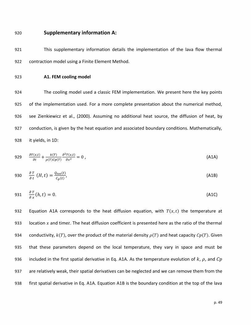
p. 49

Supplementary information A: 920

This supplementary information details the implementation of the lava flow thermal 921

contraction model using a Finite Element Method. 922

A1. FEM cooling model 923

The cooling model used a classic FEM implementation. We present here the key points 924

of the implementation used. For a more complete presentation about the numerical method, 925

see Zienkiewicz et al., (2000). Assuming no additional heat source, the diffusion of heat, by 926

conduction, is given by the heat equation and associated boundary conditions. Mathematically, 927

it yields, in 1D: 928

𝜕𝑇(𝑥,𝑡)

𝜕𝑡+

𝑘(𝑇)

𝜌(𝑇)𝐶𝑝(𝑇)

𝜕2𝑇(𝑥,𝑡)

𝜕𝑥2 = 0 , (A1A) 929

𝜕 𝑇

𝜕 𝑡 (𝐻, 𝑡) =

𝑄𝑡𝑜𝑡(𝑡)

𝐶𝑝(𝑡), (A1B) 930

𝜕 𝑇

𝜕 𝑥(ℎ, 𝑡) = 0. (A1C) 931

Equation A1A corresponds to the heat diffusion equation, with 𝑇(𝑥, 𝑡) the temperature at 932

location 𝑥 and time𝑡. The heat diffusion coefficient is presented here as the ratio of the thermal 933

conductivity, 𝑘(𝑇), over the product of the material density 𝜌(𝑇) and heat capacity 𝐶𝑝(𝑇). Given 934

that these parameters depend on the local temperature, they vary in space and must be 935

included in the first spatial derivative in Eq. A1A. As the temperature evolution of 𝑘, 𝜌, and 𝐶𝑝 936

are relatively weak, their spatial derivatives can be neglected and we can remove them from the 937

first spatial derivative in Eq. A1A. Equation A1B is the boundary condition at the top of the lava 938

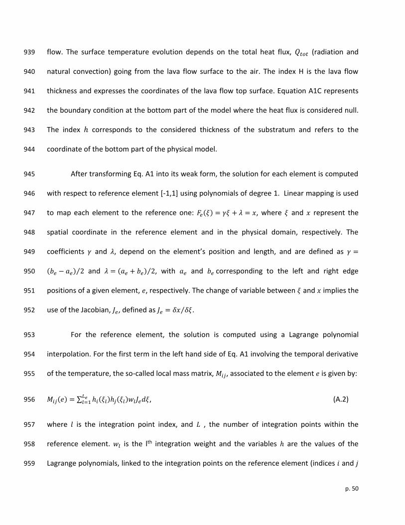
p. 50

flow. The surface temperature evolution depends on the total heat flux, 𝑄𝑡𝑜𝑡 (radiation and 939

natural convection) going from the lava flow surface to the air. The index H is the lava flow 940

thickness and expresses the coordinates of the lava flow top surface. Equation A1C represents 941

the boundary condition at the bottom part of the model where the heat flux is considered null. 942

The index ℎ corresponds to the considered thickness of the substratum and refers to the 943

coordinate of the bottom part of the physical model. 944

After transforming Eq. A1 into its weak form, the solution for each element is computed 945

with respect to reference element [-1,1] using polynomials of degree 1. Linear mapping is used 946

to map each element to the reference one: 𝐹𝑒(𝜉) = 𝛾𝜉 + 𝜆 = 𝑥, where 𝜉 and 𝑥 represent the 947

spatial coordinate in the reference element and in the physical domain, respectively. The 948

coefficients 𝛾 and 𝜆, depend on the element’s position and length, and are defined as 𝛾 =949

(𝑏𝑒 − 𝑎𝑒) 2⁄ and 𝜆 = (𝑎𝑒 + 𝑏𝑒) 2⁄ , with 𝑎𝑒 and 𝑏𝑒 corresponding to the left and right edge 950

positions of a given element, 𝑒, respectively. The change of variable between 𝜉 and 𝑥 implies the 951

use of the Jacobian, 𝐽𝑒, defined as 𝐽𝑒 = 𝛿𝑥 𝛿𝜉⁄ . 952

For the reference element, the solution is computed using a Lagrange polynomial 953

interpolation. For the first term in the left hand side of Eq. A1 involving the temporal derivative 954

of the temperature, the so-called local mass matrix, 𝑀𝑖𝑗, associated to the element 𝑒 is given by: 955

𝑀𝑖𝑗(𝑒) = ∑ ℎ𝑖(𝜉𝑙)ℎ𝑗(𝜉𝑙)𝑤𝑙𝐽𝑒𝑑𝜉𝐿𝑒𝑙=1 , (A.2) 956

where 𝑙 is the integration point index, and 𝐿 , the number of integration points within the 957

reference element. 𝑤𝑙 is the lth integration weight and the variables ℎ are the values of the 958

Lagrange polynomials, linked to the integration points on the reference element (indices 𝑖 and 𝑗 959

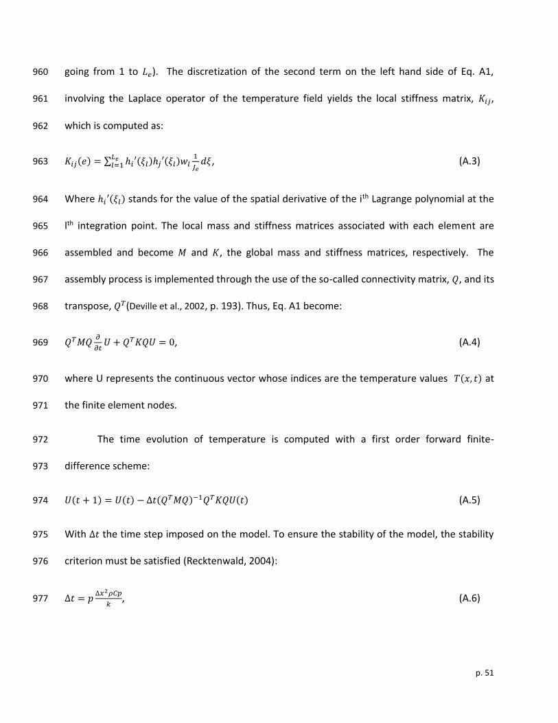
p. 51

going from 1 to 𝐿𝑒). The discretization of the second term on the left hand side of Eq. A1, 960

involving the Laplace operator of the temperature field yields the local stiffness matrix, 𝐾𝑖𝑗, 961

which is computed as: 962

𝐾𝑖𝑗(𝑒) = ∑ ℎ𝑖′(𝜉𝑙)ℎ𝑗′(𝜉𝑙)𝑤𝑙1

𝐽𝑒𝑑𝜉

𝐿𝑒𝑙=1 , (A.3) 963

Where ℎ𝑖′(𝜉𝑙) stands for the value of the spatial derivative of the ith Lagrange polynomial at the 964

lth integration point. The local mass and stiffness matrices associated with each element are 965

assembled and become 𝑀 and 𝐾, the global mass and stiffness matrices, respectively. The 966

assembly process is implemented through the use of the so-called connectivity matrix, 𝑄, and its 967

transpose, 𝑄𝑇(Deville et al., 2002, p. 193). Thus, Eq. A1 become: 968

𝑄𝑇𝑀𝑄𝜕

𝜕𝑡𝑈 + 𝑄𝑇𝐾𝑄𝑈 = 0, (A.4) 969

where U represents the continuous vector whose indices are the temperature values 𝑇(𝑥, 𝑡) at 970

the finite element nodes. 971

The time evolution of temperature is computed with a first order forward finite-972

difference scheme: 973

𝑈(𝑡 + 1) = 𝑈(𝑡) − ∆𝑡(𝑄𝑇𝑀𝑄)−1𝑄𝑇𝐾𝑄𝑈(𝑡) (A.5) 974

With ∆𝑡 the time step imposed on the model. To ensure the stability of the model, the stability 975

criterion must be satisfied (Recktenwald, 2004): 976

∆𝑡 = 𝑝∆𝑥2𝜌𝐶𝑝

𝑘, (A.6) 977

p. 52

with the stability coefficient, p<0.5, and, ∆𝑥, the lowest distance between two finite element 978

nodes in the physical domain. 979

A2. Implementation of boundary conditions 980

At the bottom of the substratum, a Neumann boundary condition is imposed, meaning 981

that there is no heat flux (𝜕 𝑇 𝜕⁄ 𝑥 = 0). At the lava flow surface, we used a Dirichlet boundary 982

condition by imposing a temperature, at each time step. Carrying out the Neumann boundary 983

condition in the finite element model is natural and does not require special treatment. On the 984

contrary, the Dirichlet boundary condition has to be enforced at each time step, with the 985

desired temperature being input. This temperature is initially fixed at that of the lava flow, and 986

then decreases with time due to radiative and convective heat loss to the air. The natural 987

convective and radiative heat fluxes at the surface of the lava flow are computed as in Patrick et 988

al., (2004). The surface temperature is then computed using a first order finite difference 989

scheme, function of the total surface heat flux, 𝑄𝑡𝑜𝑡 as: 990

𝑇𝑠𝑢𝑟𝑓(𝑡 + ∆𝑡) = 𝑇𝑠𝑢𝑟𝑓 + ∆𝑡𝑄𝑡𝑜𝑡

𝐶𝑝. (A.7) 991

At the initiation of the simulation, as the surface temperature decreases rapidly, the 992

time step required to correctly sample the variations of the Dirichlet boundary condition at the 993

top of the lava flow using Eq. A7 is smaller than for Eq. A5. Thus, we limit the time step to have, 994

at maximum, a change of surface temperature of 1% for each iteration, before updating the 995

total heat flux. Thus, time steps increase at the beginning of the simulation, with the decrease 996

of the surface temperature, before reaching the time step imposed by Eq A6. 997

998

p. 53

A3. Thermal compaction approach 999

The thermal contraction or expansion of elements are computed, at each time step, 1000

after a new temperature field has been computed. The length evolution of an element depends 1001

on its temperature change. As the elements are sampled by several nodes, an average of the 1002

temperature, 𝑇�́�, is needed and computed as: 1003

𝑇�́� = ∑ 𝑇(𝑙, 𝑡)𝑤𝑙𝐿𝑒𝑙 . (A.8) 1004

The length evolution of each element, 𝑑ℎ𝑒, is computed as a function of the temporal evolution 1005

of the element’s average temperature with: 1006

𝑑 ℎ𝑒

𝑑 𝑡= 𝛽

1+𝜈

1−𝜈 𝜕 𝑇

𝜕 𝑡 , (A.9) 1007

with ℎ𝑒, the element length, 𝛽, the thermal expansion coefficient and 𝜈, the Poisson coefficient. 1008

Eq. (A.9) is discretized using a first order finite difference scheme in time, and yields: 1009

𝑑ℎ𝑒(𝑡) = ℎ𝑒(𝑡 − ∆𝑡)𝛽1+𝜈

1−𝜈(𝑇�́�(𝑡) − 𝑇�́�(𝑡 − ∆𝑡)), (A.10) 1010

With ℎ𝑒 the element length and 𝑇�́� its average temperature. After computing the new elements 1011

length and integration point positions, the cooling model is adjusted by updating 𝐽𝑒, 𝐹𝑒, 𝑀 and 1012

𝐾. The elements’ densities, heat capacities and thermal conductivities are also updated, at each 1013

time step, with their new average temperature. 1014

1015

A4. Cooling model error and effect of the grid deformation 1016

A4.1 Evaluation of the error 1017

p. 54

The precision of a numerical model depends on the spatial and temporal step used. 1018

Here, Eq. A6 imposes that each time step depends on a space step and the stability coefficient. 1019

The space step itself depends on the number of elements chosen. Thus, the two variables 1020

controlling the accuracy of the numerical method are the number of elements (space accuracy) 1021

and the stability coefficient (time accuracy). We tested the accuracy of the cooling model by 1022

considering a uniform medium, with a constant conductivity, heat capacity and density, and 1023

neglecting the thermal contraction of elements. An initial temperature distribution inside the 1024

medium is set with a sinusoidal function, which has an analytical solution: 𝑈(𝑥, 𝑡) =1025

𝑠𝑖𝑛(𝜋𝑥)𝑒−(𝑘 𝜌⁄ 𝐶𝑝)𝑡. The model error is estimated by computing the average temperature 1026

difference between the numerical and analytical solutions after one iteration. Figure A1 shows 1027

that the absolute average error decreases with the stability coefficient and with an increase in 1028

the number of elements. The slope of the two curves illustrates that the method is accurate to 1029

the second order in space (Fig. A1A) and the first order in time (Fig. A1B). We found that for our 1030

case the numerical solution is always hotter than the analytical one. 1031

A4.2 Effect of the grid deformation 1032

All previous studies using numerical modeling of lava flow thermo-elastic contractions 1033

neglected the potential effects of grid deformation on heat diffusion and in turn to the 1034

estimated displacements (Wittmann et al., 2017). This was either a choice made by the authors 1035

or was imposed by the numerical method employed. The advantage of using FEM, is that it 1036

takes into account the thermally induced grid deformations on the heat diffusion because the 1037

grid points are allowed to move. In order to quantify the actual effect of grid deformation, we 1038

performed two simulations with the same initial condition and input parameters. The first 1039

p. 55

simulation takes the grid deformation into account in the cooling model, whereas the second 1040

one ignores it. Figure A2 displays the evolution of the differences between the two simulations 1041

on the vertical subsidence rate. It shows that the deformation rate difference is not constant 1042

with time. It starts to increase at the beginning of the simulation and reaches a maximum of 1043

~3.5% after 1 month. This difference then decreases and tends to stabilize after about ten 1044

months to a value ~2.6%. It should be noted that if grid deformation is not taken into account, 1045

then the deformation rate is always underestimated. Our results indicate that ignoring grid 1046

deformation seems a reasonable assumption for characterizing lava flow behavior given the 1047

uncertainties of the thermal properties. 1048

Supplementary references: 1049

Deville, M.O., Fischer, P.F., Mund, E.H., 2002. High-order methods for incompressible fluid flow. 1050

Cambridge university press. 1051

Recktenwald, G.W., 2004. Finite-difference approximations to the heat equation. Mech. Eng. 10, 1–27. 1052

Zienkiewicz, O.C., Taylor, R.L., Taylor, R.L., 2000. The finite element method: solid mechanics. 1053

Butterworth-heinemann. 1054

1055

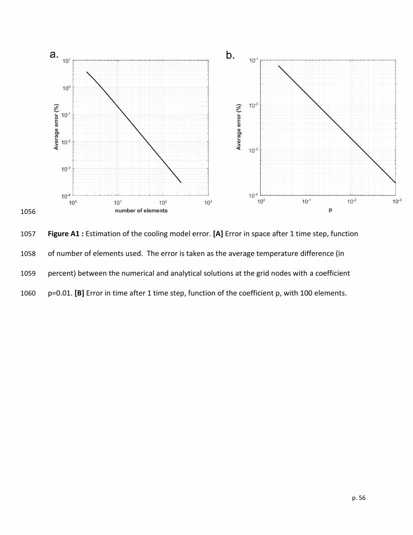
p. 56

1056

Figure A1 : Estimation of the cooling model error. [A] Error in space after 1 time step, function 1057

of number of elements used. The error is taken as the average temperature difference (in 1058

percent) between the numerical and analytical solutions at the grid nodes with a coefficient 1059

p=0.01. [B] Error in time after 1 time step, function of the coefficient p, with 100 elements. 1060

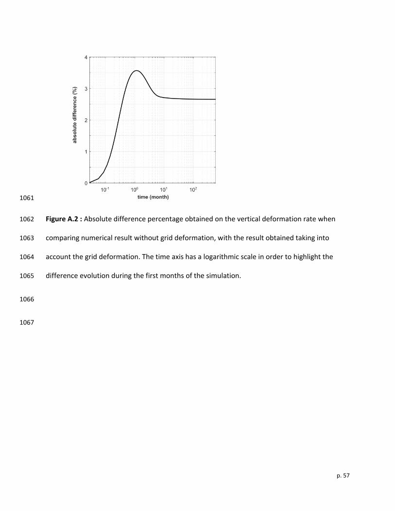
p. 57

1061

Figure A.2 : Absolute difference percentage obtained on the vertical deformation rate when 1062

comparing numerical result without grid deformation, with the result obtained taking into 1063

account the grid deformation. The time axis has a logarithmic scale in order to highlight the 1064

difference evolution during the first months of the simulation. 1065

1066

1067