Position and Velocity Tracking in Mobile Networks Using Particle and Kalman Filtering With Comparison

IEEE TRANSACTIONS ON VEHICULAR TECHNOLOGY, VOL. 57, NO. 2, MARCH 2008 1001

Position and Velocity Tracking in MobileNetworks Using Particle and Kalman

Filtering With ComparisonMohammed M. Olama, Seddik M. Djouadi, Ioannis G. Papageorgiou, and Charalambos D. Charalambous

Abstract—This paper presents several methods based on signalstrength and wave scattering models for tracking a user. Thereceived-signal level method is first used in combination withmaximum likelihood (ML) estimation and triangulation to obtainan estimate of the location of the mobile. Due to nonline-of-sightconditions and multipath propagation environments, this estimatelacks acceptable accuracy for demanding services, as the numer-ical results reveal. The 3-D wave scattering multipath channelmodel of Aulin is employed, together with the recursive nonlinearBayesian estimation algorithms to obtain improved location esti-mates with high accuracy. Several Bayesian estimation algorithmsare considered, such as the extended Kalman filter (EKF), theparticle filter (PF), and the unscented PF (UPF). These algorithmscope with nonlinearities in order to estimate mobile location andvelocity. Since the EKF is very sensitive to the initial state, wepropose the use of the ML estimate as the initial state of theEKF. In contrast to the EKF tracking approach, the PF and UPFapproaches do not rely on linearized motion models, measurementrelations, and Gaussian assumptions. Numerical results are pre-sented to evaluate the performance of the proposed algorithmswhen the measurement data do not correspond to the ones gen-erated by the model. This shows the robustness of the algorithmbased on modeling inaccuracies.

Index Terms—Kalman filtering, location tracking, maximumlikelihood estimation (MLE), multipath fading channels, particlefiltering.

I. INTRODUCTION

THE NEED for an efficient and accurate mobile station(MS) positioning system is growing day by day. This

has been stressed by a federal order that has been issuedby the Federal Communications Commission (FCC), whichmandates all wireless service providers to provide public safetyanswering points with information to locate an emergency 911caller with an accuracy of 100 m for 67% of the cases [1].

Manuscript received October 4, 2005; revised September 23, 2006,April 6, 2007, and June 12, 2007. The review of this paper was coordinatedby Dr. R. Klukas.

M. M. Olama and S. M. Djouadi are with the Electrical and ComputerEngineering Department, University of Tennessee, Knoxville, TN 37996 USA(e-mail: [email protected]; [email protected]).

I. G. Papageorgiou is with the Electrical and Computer Engineering De-partment, University of Cyprus, 1678 Nicosia, Cyprus and also with theCyprus Telecommunications Authority, CY-1396 Nicosia, Cyprus (e-mail:[email protected]).

C. D. Charalambous is with the Electrical and Computer EngineeringDepartment, University of Cyprus, 1678 Nicosia, Cyprus (e-mail: [email protected]).

Color versions of one or more of the figures in this paper are available onlineat http://ieeexplore.ieee.org.

Digital Object Identifier 10.1109/TVT.2007.906370

It is also expected that the FCC will tighten its requirementsin the near future [2]. Many other applications, such as ve-hicle fleet management, location sensitive billing, intelligenttransport systems, fraud protection, and mobile yellow pages,have driven the cellular industry to research new and promisingtechnologies for MS positioning.

The problem of determining the location and velocity of anMS has extensively been studied in the last few years. The cur-rent standards for estimating location and velocity are mostlybased on time signal information, such as time difference ofarrival (TDOA), enhanced observed time differences (E-OTD),observed TDOA (OTDOA), global positioning system (GPS),etc. [3]–[7]. However, not all of these methods meet the nec-essary needs that are imposed by certain services. In addition,most of them require a new hardware since localization is notinherent in the current wireless systems; for instance, GPSdemands a new receiver, and TDOA, E-OTD, and OTDOA re-quire additional location measurement units in the network [8].Adding extra hardware means extra cost for implementation,which can be reflected on both consumers and operators. Re-searchers have also suggested several MS location methodsbased on signal power measurements, such as in [9] and [10],where a certain minimization problem is numerically solved toget an initial estimate of the MS position, and then, a smoothingprocedure such as linear regression [9] or the Kalman filter [10]is applied to obtain a more accurate estimate.

In this paper, several MS tracking methods based on maxi-mum likelihood estimation (MLE) [11] and recursive nonlinearBayesian estimation (RNBE) algorithms, such as the extendedKalman filter (EKF) [12], the particle filter (PF) [13], and theunscented PF (UPF) [14], are proposed. The MLE algorithmemploys the average received-power measurements based onthe lognormal propagation channel model to obtain an initialMS location estimate [3], [16]. These measurements are readilyavailable through network measurement reports (NMRs) orradio measurements (in idle or active mode) for any MS unitin 2G and 3G cellular networks. The RNBE algorithms employthe instantaneous electric field measurements based on the 3-Dmultipath channel model of Aulin [15] to account for multipathand nonline-of-sight (NLOS) characteristics of the wirelesschannel, as well as the dynamicity of the MS. The receivedinstantaneous electric field of this model is a nonlinear functionof the position and velocity of the MS. The EKF approachis based on linearizing the nonlinear system model aroundthe previous estimate and, therefore, is very sensitive to the

0018-9545/$25.00 © 2008 IEEE

1002 IEEE TRANSACTIONS ON VEHICULAR TECHNOLOGY, VOL. 57, NO. 2, MARCH 2008

initial state. This motivates the use of the ML estimate of theMS location as an initial state of the EKF. Particle-filteringapproaches approximate the optimal solution numerically basedon the physical model, rather than applying an optimal filterto an approximate model, such as in the EKF. They providegeneral solutions to many problems where linearization andGaussian approximations are intractable or are yielding lowperformance. The more nonlinear the model is or the more non-Gaussian the noise is, the more potential PFs have, especiallyin applications where computational power is rather cheap andthe sampling rate is moderate. In this paper, particle filtering isimplemented for the generic PF and the more recent UPF.

Aulin’s model postulates knowledge of the instantaneousreceived field at the MS, which is obtained through the circuitryof the mobile unit. The proposed RNBE algorithms take intoaccount NLOS condition as well as multipath propagationenvironments. They require only one base station (BS) toestimate the MS location instead of at least three BSs, as foundin the literature [10], [16]. However, an initial MS locationestimate that requires at least three BSs, such as the MLEand triangulation method, will improve the convergence of theRNBE filter. Particle filtering has been used in several trackingwireless applications [17]–[20], but the channel models that areused do not take into account the multipath properties of thewireless channel. To the best of our knowledge, the utilizationof the PF and/or the UPF, together with the classical wirelesschannel model, to extract the MS location and velocity is new.The performance of the proposed algorithms is numericallycomputed and is in the presence of parameter uncertainty.Numerical results indicate that the proposed UPF algorithm ishighly accurate and superior to other approaches.

The main contribution of this paper is to develop MS locationand velocity estimation algorithms, which use Aulin’s 3-Dwave scattering model and are based on particle filtering. Theperformance is compared with that of the EKF. The choice ofthis channel model is to account for the multipath properties andNLOS of wireless networks. These methods support existingnetwork infrastructure and channel signaling and only use oneBS. Moreover, simulations are performed under uncertainties inthe model parameters of the channel to evaluate the robustnessof the algorithm.

This paper is structured as follows. In Section II, wedescribe the mathematical models for the location and velocityestimation algorithms. The MLE and EKF approaches forMS location estimation are presented in Sections III and IV,respectively. The PF and UPF approaches for MS locationand velocity estimation, which are the main contribution ofthis paper, are presented in Sections V and VI, respectively.In Section VII, we present numerical results and evaluate therobustness of the proposed algorithms to uncertainties dueto random variations in the channel parameters. Section VIIIprovides the concluding remarks.

II. SYSTEM MATHEMATICAL MODELS

A. Lognormal Propagation Channel Model

Here, we consider a 2-D geometry, with the MS lo-cated at (x0, y0) and the BSs located at ((xBS1 , yBS1), (xBS2 ,

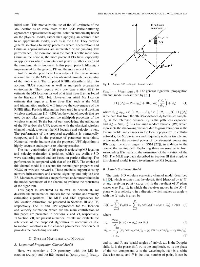
Fig. 1. Aulin’s 3-D multipath channel model.

yBS2), . . . , (xBSB, yBSB

)). The general lognormal propagationchannel model is described by [21]

PLsb(db) = PL (d0b

) + 10εb log(

db

d0b

)+ Xs

b (1)

where db ≥ d0b, s ∈ {1, 2, . . . , S}, b ∈ {1, 2, . . . , B}, PLs

b(db)is the path loss from the bth BS at distance db for the sth sample,d0b

is the reference distance, εb is the path loss exponent,and Xs

b ∼ N(0;σ2b ) is a Gaussian random variable (RV) which

represents the shadowing variance due to gross variations in theterrain profile and changes in the local topography. In cellularnetworks, the MS preserves and frequently updates (in idle andactive mode) the received power of the strongest nonservingBSs (e.g., the six strongest in GSM [22]), in addition to theone of the serving cell. Exploiting these measurements fromsurrounding BSs leads to the estimation of the location of theMS. The MLE approach described in Section III that employsthis channel model is used to estimate the MS location.

B. Aulin’s Scattering Model

The basic 3-D wireless scattering channel model describedin [15], which assumes that the electric field [denoted by E(t)]at any receiving point (x0, y0, z0) is the resultant of P planewaves (see Fig. 1), in which the receiver moves in the X−Yplane with a velocity v in a direction which makes an angle γwith the X-axis, is given by

E(t) =P∑

n=1

En(t) =P∑

n=1

rn cos(ωct + ωnt + θn) + e(t) (2)

where

ωn =2πυ

λ(cos(γ − αn) cos βn) (3)

θn = −2π

λ(x0 cos αn cos βn + y0 sinαn cos βn + z0 sinβn)

+ φn (4)

and αn and βn are spatial angles of arrival, ωn is the Dopplershift, θn is the phase shift, rn is the amplitude, φn is the phaseof the nth component, λ is the wavelength, e(t) is a whiteGaussian noise, and P is the total number of paths. It can be

OLAMA et al.: POSITION AND VELOCITY TRACKING IN MOBILE NETWORKS 1003

seen from (3) and (4) that the Doppler and phase shifts dependon the velocity and location of the receiver, respectively.

Clearly, (2) assumes transmission of a narrowband signal.This assumption is valid only when the signal bandwidth issmaller than the coherence bandwidth of the channel. Never-theless, the aforementioned model is not restrictive since it canbe modified to represent a wideband transmission by includingmultiple time-delayed echoes. In this case, the delay spreadhas to be estimated. A sounding device is usually dedicated inestimating the time delay of each discrete path, such as the Rakereceiver [23].

It can be seen that the noisy instantaneous received field in(2) parametrically depends on the location and velocity of thereceiver. Consequently, this expression is used to estimate theMS location and velocity by using the EKF, the PF, and/orthe UPF. Next, we formulate the location estimation as afiltering problem in state-space form [24]. The general form,once discretized, is given by

xk = f(xk−1,wk−1)zk =h(xk,vk) (5)

where f(., .) and h(., .) are known vector functions, k is theestimation step, zk is the output measurements at time step k,and xk is the system state at time step k and must not be con-fused with location coordinates. Furthermore, wk and vk are thediscrete zero-mean, independent state, and measurement noiseprocesses with covariance matrices Q and R, respectively.

Now, let xk = [xk, xk, yk, yk]T denote the state of the MS attime k, where xk and yk are the Cartesian coordinates of theMS, and xk and yk are the velocities of the MS in the X and Ydirections, respectively. We choose the case where the velocityof the MS is not known and is subject to unknown accelerations.The dynamics of the MS can be written as [17]

xk =

xk

xk

yk

yk

=

1 ∆k 0 00 1 0 00 0 1 ∆k

0 0 0 1

xk−1

xk−1

yk−1

yk−1

+

∆2k/2 0

∆k 00 ∆2

k/20 ∆k

[wk−1,1

wk−1,2

]

(6)

where ∆k is a (possibly nonuniform) measurement intervalbetween time k − 1 and k.

The measurement equation can be found from Aulin’s scat-tering model (2)–(4), which can be written in discrete form as

zk = h(xk, vk) =P∑

n=1

rnkcos (ωctk + ωnk

tk + θnk) + v(tk)

(7)where

ωnk=

2π√

x2k + y2

k

λ(cos (γk − αnk

) cos βnk) (8)

θnk=

−2π

λ(xk cos αnk

cos βnk+ yk sin αnk

cos βnk

+ z0 sin βnk) + φnk

. (9)

Clearly, the measurement equation h(., .) is a nonlinearfunction of the state-space vector, as observed in (7)–(9). Ifwe assume approximate knowledge of the channel, which is at-tainable either through channel estimation at the receiver (e.g.,GSM receiver) or through various estimation techniques (e.g.,least squares and ML), then this problem falls under the broadarea of nonlinear parameter estimation from noisy data whichcan be solved using the RNBE algorithms. These algorithmswill be discussed in Sections IV–VI. The MLE algorithm thatemploys the lognormal propagation channel model is discussedin the next section.

III. MLE APPROACH FOR MS LOCATION ESTIMATION

In this section, the MLE method that employs the log-normal propagation channel model described in Section II-Ais considered for the MS location estimation. This methodexploits the received-power measurements at the MS, which areavailable from NMRs. Thus, we write the likelihood functionand then maximize it with respect to the distances θ = d =(d1, d2, . . . , dB) from each BS, where θ is the parameter tobe estimated. The ML estimator, which is denoted by θ = d =(d1, d2, . . . , dB), represents the most possible MS/BS distancesbased on the measurements available at the MS.

Consider the measurement vector for the sth samplefrom all BSs, which is denoted by PLs(d) =(PLs

1(d1), PLs2(d2), . . . , PLs

B(dB)). The distribution functionfor this vector is the B-variate normal distribution, which isgiven by

p (PLs(d)|θ)=(2π)−B/2 (det(Σs))−1/2

× exp(− 1

2

( (PLs(d)−PL

s(d)

)T

× Σ−1s(

PLs(d)−PLs(d)

) ))(10)

where PLs(d) ∼ NB(PLs(d);Σs), PL

s(d) = (PL

s1(d1),

PLs2(d2), . . . , PL

sB(dB)) is the mean path loss from each BS,

and Σs is the covariance matrix. By assuming that the noise isindependent identically distributed (i.i.d.), then the logarithmlikelihood function is the log product of the sample likelihoodfunctions given by

L (θ|PLs(d)) = log

(1

(2π)SB/2 (det(Σs))S/2

)

−S∑

s=1

((PLs(d) − PL

s(d)

)T

×Σ−1s

2

(PLs(d) − PL

s(d)

))(11)

1004 IEEE TRANSACTIONS ON VEHICULAR TECHNOLOGY, VOL. 57, NO. 2, MARCH 2008

where S is the total number of samples. By maximizing (11)first with respect to PL

s(d), the score function yields

∧PLb(db) =

1S

S∑s=1

PLsb(db) ∀b ∈ {1, 2, . . . , B}. (12)

Solving for d using the invariance property of the MLE [11], itcan be shown that

db = 10

{1

10εb

[1S

S∑s=1

PLsb(db)−PL(d0b

)

]}(13)

is the MLE for the distance of the bth BS from the MS. Next,we perform triangulation using the least-squares error method[25] to estimate the MS location (x0, y0) by solving

arg minx0,y0

{B∑

b=1

(db − db)2}

. (14)

The performance of this location estimation algorithm is dis-cussed through numerical results and compared to the followingalgorithms in Section VII.

In the next section, the EKF approach that employs the chan-nel model of Aulin to estimate the MS location and velocity isdiscussed.

IV. EKF APPROACH FOR MS LOCATION AND

VELOCITY ESTIMATION

Consider the general discrete-time dynamical system modeldescribed in (5). Let the known probability density functions(pdfs) of the process noise wk and the measurement noise vk

be p(wk) and p(vk), respectively. As usual, wk and vk areassumed to be mutually independent. The set of entire mea-surements from the initial time step to time step k is denotedby Zk = {zi}k

i=1. The distribution of the initial condition x0 isassumed to be given by p(x0|Z0) = p(x0).

The EKF is based on linearizing the nonlinear system modelsaround the previous estimate. The general algorithm for thediscrete EKF can be described by the time-update equations,which are given as [12]

xk = f(xk−1, 0)Pk =AkPk−1AT

k + WkQk−1WTk (15)

and the measurement-update equations are given as

Kk = PkHTk

[HkPkHT

k + VkRkVTk

]−1

xk = xk + Kk (zk − h(xk, 0))Pk = (I − KkHk)Pk (16)

where Ak, Wk, Vk, and Hk are shown in (17) at the bottomof the page, K is the gain matrix, P is the estimation error

Ak =∂f∂x

(xk−1, 0) =

1 ∆k 0 00 1 0 00 0 1 ∆k

0 0 0 1

Wk =∂f∂w

(xk−1, 0) =

∆2k/2 0

∆k 00 ∆2

k/20 ∆k

Vk =∂h

∂v(xk, 0) = 1

Hk =∂h

∂x(xk, 0) = [H1k H2k H3k H4k]

H1k =P∑

n=1

[rnk

sin (ωctk + ωnktk + θnk

)(

2π

λcos (αnk

) cos (βnk))]

H2k =P∑

n=1

−rnk

sin (ωctk + ωnktk + θnk

)(

2πt

λ√

x2k+y2

k

cos (βnk))

(xk cos (γk − αnk) + yk sin (γk − αnk

))

H3k =P∑

n=1

[rnk

sin (ωctk + ωnktk + θnk

)(

2π

λsin (αnk

) cos (βnk))]

H4k =P∑

n=1

−rnk

sin (ωctk + ωnktk + θnk

)(

2πt

λ√

x2k+y2

k

cos (βnk))

(yk cos (γk − αnk) − xk sin (γk − αnk

))

(17)

OLAMA et al.: POSITION AND VELOCITY TRACKING IN MOBILE NETWORKS 1005

covariance, and γk = arctan(yk/xk). The notation xk denotesthe a priori state estimate at time step k, and xk denotes thea posteriori state estimate when given measurement zk. Pk andPk are similarly defined.

As in any nonlinear estimation problem, the convergenceof the EKF to the true value of the location depends onthe initial parameter value; therefore, we first develop theMLE method to obtain an initial estimator of adequate accu-racy for the EKF. This hybrid algorithm, as numerical resultsindicate, has improved accuracy for the final MS locationestimate.

The aforementioned EKF utilizes the first term in aTaylor expansion of the nonlinear measurement model in (7).It always approximates p(xk|Zk) by using a Gaussian dis-tribution. However, if the true density is non-Gaussian, then aGaussian model may not precisely describe it. In such cases,PFs yield an improvement in performance in comparison tothat of an EKF. The design of the PF is discussed in the nextsection.

V. PF APPROACH FOR MS LOCATION AND

VELOCITY ESTIMATION

The PF is a technique for the implementation of a recursiveBayesian filter by Monte Carlo simulations. The key idea isto represent the required posterior density function with aset of random samples {xk(j)}N

j=1 with associated weights{ωk(j)}N

j=1 and to compute estimates based on these samplesand weights. In this case, the posterior density at time k can beapproximated as

p(xk|Zk) ≈N∑

j=1

ωk(j)δ (xk − xk(j)) . (18)

We therefore have a discrete weighted approximation to the trueposterior p(xk|Zk). The weights are chosen using the principleof importance sampling [26]

ωk(j) ∝ p (zk|xk(j)) p (xk(j)|xk−1(j))q (xk(j)|xk−1(j), zk)

(19)

where q(xk(j)|xk−1(j), zk) is the importance proposal distribution function that generates the samples {xk(j)}N

j=1. Thechoice of this distribution function is one of the most crit-ical design issues, and it determines the type of the PF.The optimal proposal distribution function that minimizes thevariance of the weights conditioned on xk−1(j) and zk isq(xk|xk−1(j), zk)opt = p(xk|xk−1(j), zk) [26].

However, analytical evaluation of the optimal proposal func-tion is not possible for many models, and thus, it has to beapproximated using local linearization [26] or the unscentedtransformation [14]. In this paper, the unscented transformationmethod is considered, and the resulting filter is called the UPF,which is described in Section VI.

Nonetheless, the most popular choice of proposal func-tion is the transition prior q(xk|xk−1(j), zk) = p(xk|xk−1(j)).This filter is called the generic PF and is discussed herein.

Although this choice of proposal function results in higherMonte Carlo variations than the optimal, it is usually simple toimplement.

The time-update stage of the generic PF [27] is performed bypassing the random samples {xk−1(j)}N

j=1 through the systemmodel (6) to obtain the time-updated samples {xk(j)}N

j=1. Thetime-updated samples are obtained by

xk(j) = f (xk−1(j),wk−1(j)) (20)

where wk−1(j) is a sample drawn from the pdf p(wk−1) of thesystem noise. The samples {xk(j)}N

j=1 are distributed as thetime-updated pdf p(xk|Zk−1).

The measurement-update stage can be described by substi-tuting the choice of proposal distribution q(xk|xk−1(j), zk) =p(xk|xk−1(j)) into (19) and normalizing, which yields

ωk(j) =p (zk|xk(j))∑N

j=1 p (zk|xk(j)). (21)

We define a discrete density over {xk(j)}Nj=1 with proba-

bility mass ωk(j) associated with each sample xk(j). Then,we get the measurement-update samples {xk(j)}N

j=1 through aresampling process such that Pr{xk(i) = xk(j)} = ωk(j) forany i. Several resampling schemes are presented in the litera-ture, such as systematic [28], stratified, and residual resampling[29]. However, the specific choice of resampling scheme doesnot significantly affect the performance of the PF. Therefore,systematic resampling is used in all of the experiments inSection VII since it is simple to implement. The estimate ofthe PF at time k is chosen to be the mean of the samples{xk(j)}N

j=1.In the next section, an approximate version of the optimal

proposal distribution is considered in order to have a moreaccurate MS location estimate.

VI. UPF APPROACH FOR MS LOCATION AND

VELOCITY ESTIMATIONS

The UPF results from using a scaled unscented transforma-tion (SUT) method to approximate the optimal proposal dis-tribution within a PF framework. The SUT provides moreaccurate approximation than linearization methods [14]. Inparticular, the SUT accurately calculates the posterior covari-ance to the third order, whereas linearization methods such asthe EKF rely on a first-order biased approximation. The SUTmethod is introduced next.

A. SUT Method

The SUT method still approximates the proposal distributionby a Gaussian distribution, but it is specified using a minimalset of deterministically chosen sample points. These samplepoints completely capture the true mean and covariance of theGaussian distribution, and when propagated through the truenonlinear system, they accurately capture the posterior meanand covariance to the third order for any nonlinearity.

1006 IEEE TRANSACTIONS ON VEHICULAR TECHNOLOGY, VOL. 57, NO. 2, MARCH 2008

Consider the state equation described in (5). For simplicity,let xk = f(xk−1), where xk−1 is an nx dimensional randomvector, and assume that xk−1 has mean xk−1 and covariancePk−1. Then, a set of 2nx + 1 weighted samples or sigmapoints Si = {Wi,Xi} are deterministically chosen so that theycompletely capture the true mean and covariance of the priorrandom vector xk−1. A selection scheme that satisfies thisrequirement is [14]

χ0k−1 =xk−1

χik−1 =xk−1+

(√(nx+λ)Pk−1

)i, i=1, . . . , nx

χik−1 =xk−1−

(√(nx+λ)Pk−1

)i, i=nx+1, . . . , 2nx

W(m)0 =λ/(nx+λ)

W(c)0 =λ/(nx+λ)+(1−α2+β)

W(m)i =W

(c)i = 1/ {2(nx+λ)} , i=1, . . . , 2nx (22)

where λ = α2(nx + κ) − nx; α, β, and κ are scaling parame-ters; and (

√(nx + λ)Pk−1)i is the ith row or column of the

matrix square root of (nx + λ)Pk−1. Each sigma point is nowpropagated through the nonlinear function Xi

k = f(Xik−1), i =

0, . . . , 2nx. The estimated mean and covariance of xk arecomputed as follows:

xk =2nx∑i=0

W(m)i χi

k

Pk =2nx∑i=0

W(c)i

{χi

k − xk

} {χi

k − xk

}T. (23)

These estimates of the mean and covariance are accurate to thethird order for any nonlinear function. In comparison, the EKFonly accurately calculates the posterior mean and covariance tothe first order, with all higher order moments truncated.

B. UPF Design

The UPF uses the same framework as the regular PF, exceptthat it approximates the optimal proposal distribution by aGaussian distribution using the SUT method. In particular, theSUT is used to generate and propagate a Gaussian proposaldistribution for each particle to get

q (xk(j)|xk−1(j), zk)opt ≈ N (xk(j),Pk(j)) (24)

and j = 1, . . . , N . That is, at time k − 1, the SUT is usedwith the new data to compute the mean and covariance of theimportance distribution for each particle. Next, the jth particleis sampled from this distribution.

The description of the UPF approach in this section is mainlybased on the study in [14]. In the implementation of the UPF,the augmented state vector is defined as the concatenation of the

original state and noise variables as xsk = [xT

k wTk vk]T. Then,

the SUT sigma point selection scheme is applied to this newaugmented state vector to calculate the corresponding sigmamatrix χa

k. The complete UPF is described as follows [14].

1) Initialization (k = 0): Draw the particles {x0(j)}Nj=1

from the prior p(x0), and set

x0(j) =E [x0(j)]

P0(j) =E[(x0(j) − x0(j)) (x0(j) − x0(j))

T]

xa0(j) =E [xa

0(j)] =[(x0(j))

T 0 0]T

Pa0(j) =E

[(xa

0(j) − xa0(j)) (xa

0(j) − xa0(j))T

]

=

P0(j) 0 0

0 Q 00 0 R

(25)

where E[.] is the expectation operator.2) Now, for k = 1, 2, . . ., the importance sampling step is

performed by the following steps.a) Calculate the sigma points

χak−1(j) =

[xa

k−1(j)xak−1(j) ±

√(na + λ)Pa

k−1(j)]. (26)

b) Perform the time-update stage as

χxk(j) = f

(χx

k−1(j),χvk−1(j)

)

xk(j) =2na∑i=0

W(m)i χx

i,k(j)

Pk(j) =2na∑i=0

W(c)i

{χx

i,k(j) − xk(j)} {

χxi,k(j) − xk(j)

}T

Zk(j) =h(χx

k(j),χnk−1(j)

)

zk(j) =2na∑i=0

W(m)i Zi,k(j). (27)

c) Perform the measurement-update stage as

Pzkzk=

2na∑i=0

W(c)i

{Zi,k(j) − zk(j)

} {Zi,k(j) − zk(j)

}T

Pxkzk=

2na∑i=0

W(c)i

{χx

i,k(j) − xk(j)} {

Zi,k(j) − zk(j)}T

Kk =PxkzkP−1

zkzk,�xk(j) = xk(j) + Kk

(zk − zk(j)

)�

Pk (j) = Pk(j) − KkPzkzkKT

k (28)

and then sample�xk (j) from q(xk(j)|xk−1(j), zk) =

N(�xk(j),

�

Pk(j)).

OLAMA et al.: POSITION AND VELOCITY TRACKING IN MOBILE NETWORKS 1007

d) Evaluate the importance weights as

ωk(j) ∝p

(zk|

�xk (j)

)p

(�xk (j)|xk−1(j)

)q(

�xk (j)|xk−1(j), zk

) (29)

and then normalize the importance weights for j =1, . . . , N .

3) Finally, a resampling process such as systematic re-sampling is performed to obtain N random particles(xk(j), Pk(j)), and the output is generated in the samemanner as that for the generic PF.

In the next section, numerical examples are presented toillustrate the accuracy of the proposed algorithms.

VII. NUMERICAL RESULTS

In this numerical example, the performance of the proposedMS location and velocity estimation algorithms is determined.We consider first the ML estimate of the MS location, in whichwe employ a typical, yet realistic, wireless communicationsimulation setup. The service area consists of a 19-cell cluster.The BSs are placed over a uniform hexagonal pattern of cellsthat are centrally equipped with omnidirectional antennas. MSsare randomly placed in the central cell, and the number ofarranged users is 1000. Path-loss exponent εb is 3.5, path-loss variance σ2

b is 8 dB, reference distance d0bis 200 m

for all b [30], cell radius is 5000 m, the number of samplesS is ten, the number of BSs for triangulation is five, radio-frequency is 900 MHz, and 100 Monte Carlo simulations wereperformed.

Next, we consider the simulation setup for the EKF, the PF,and the UPF approaches that employ Aulin’s channel model forMS location and velocity estimation. The simulation setup forthe MLE approach remains the same; it is only now that weare trying to locate a single MS. The envelope of the receivedsignal for all paths rn’s is generated as Rayleigh i.i.d. RVs witha parameter of 0.5. an, βn, and φn are generated as uniformi.i.d. RVs in [0, 2π], [0, 0.2π], and [0, 2π], respectively. The totalnumber of paths P is six (which represents urban environment).The filters have the following parameters: The number of timesteps (measurements) is 50, with ∆k = 0.1 s; the process noisecovariance Q and the measurement noise variance R are I2×2

and 0.01, respectively, where I2×2 is the 2-D identity matrix;the initial pdf of the MS position is assumed to be uniform overthe entire cell size, which represents the worst case as far aschoosing an initial pdf is considered; the initial pdf of the MSvelocity is Gaussian distributed, with a mean of 65 m/s and avariance of 10; and the number of particles is 500. The SUTparameters are set to α = 1, β = 0, and κ = 0, and finally, themean estimate of all particles is used as the final estimate. Theposition (or velocity) root mean-square error (RMSE) is usedas a performance measure and is defined as

RMSE(k) =

√√√√ 1MC

MC∑i=1

(xi

k − xtruek

)T (xi

k − xtruek

)(30)

Fig. 2. (a) Location and (b) velocity estimates of a moving MS generated bydifferent filters.

where MC is the number of performed Monte Carlo simula-tions, and xi

k is the filter position estimate (x, y)T [or velocityestimate (x, y)T] at time k in Monte Carlo run i. The overallRMSE is defined as

RMSE =

√√√√1L

L∑k=1

1MC

MC∑i=1

(xi

k − xtruek

)T(xi

k − xtruek

)(31)

where L is the total number of simulation time steps after theconvergence of the filter.

Fig. 2(a) and (b) shows one realization illustrating the conver-gence of the proposed algorithms to the real position and veloc-ity of a moving MS, respectively. Fig. 3 shows the position andvelocity RMSE for each time according to (30), respectively,and the overall position and velocity RMSEs of the convergentruns using (31) are shown in Table I.

In Fig. 3 and Table I, it can be noticed that the accuracyof the MLE approach is satisfactory. However, in realistic

1008 IEEE TRANSACTIONS ON VEHICULAR TECHNOLOGY, VOL. 57, NO. 2, MARCH 2008

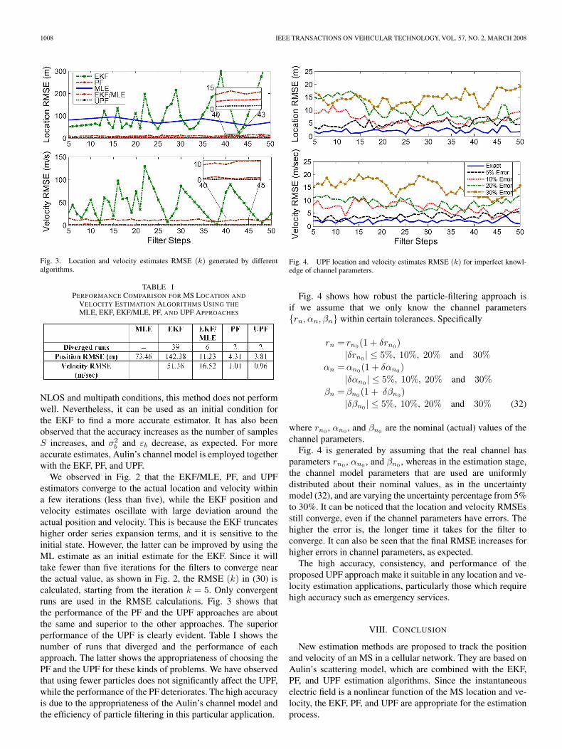
Fig. 3. Location and velocity estimates RMSE (k) generated by differentalgorithms.

TABLE IPERFORMANCE COMPARISON FOR MS LOCATION AND

VELOCITY ESTIMATION ALGORITHMS USING THE

MLE, EKF, EKF/MLE, PF, AND UPF APPROACHES

NLOS and multipath conditions, this method does not performwell. Nevertheless, it can be used as an initial condition forthe EKF to find a more accurate estimator. It has also beenobserved that the accuracy increases as the number of samplesS increases, and σ2

b and εb decrease, as expected. For moreaccurate estimates, Aulin’s channel model is employed togetherwith the EKF, PF, and UPF.

We observed in Fig. 2 that the EKF/MLE, PF, and UPFestimators converge to the actual location and velocity withina few iterations (less than five), while the EKF position andvelocity estimates oscillate with large deviation around theactual position and velocity. This is because the EKF truncateshigher order series expansion terms, and it is sensitive to theinitial state. However, the latter can be improved by using theML estimate as an initial estimate for the EKF. Since it willtake fewer than five iterations for the filters to converge nearthe actual value, as shown in Fig. 2, the RMSE (k) in (30) iscalculated, starting from the iteration k = 5. Only convergentruns are used in the RMSE calculations. Fig. 3 shows thatthe performance of the PF and the UPF approaches are aboutthe same and superior to the other approaches. The superiorperformance of the UPF is clearly evident. Table I shows thenumber of runs that diverged and the performance of eachapproach. The latter shows the appropriateness of choosing thePF and the UPF for these kinds of problems. We have observedthat using fewer particles does not significantly affect the UPF,while the performance of the PF deteriorates. The high accuracyis due to the appropriateness of the Aulin’s channel model andthe efficiency of particle filtering in this particular application.

Fig. 4. UPF location and velocity estimates RMSE (k) for imperfect knowl-edge of channel parameters.

Fig. 4 shows how robust the particle-filtering approach isif we assume that we only know the channel parameters{rn, αn, βn} within certain tolerances. Specifically

rn = rn0(1 + δrn0)|δrn0 | ≤ 5%, 10%, 20% and 30%

αn =αn0(1 + δαn0)|δαn0 | ≤ 5%, 10%, 20% and 30%

βn =βn0(1 + δβn0)|δβn0 | ≤ 5%, 10%, 20% and 30% (32)

where rn0 , αn0 , and βn0 are the nominal (actual) values of thechannel parameters.

Fig. 4 is generated by assuming that the real channel hasparameters rn0 , αn0 , and βn0 , whereas in the estimation stage,the channel model parameters that are used are uniformlydistributed about their nominal values, as in the uncertaintymodel (32), and are varying the uncertainty percentage from 5%to 30%. It can be noticed that the location and velocity RMSEsstill converge, even if the channel parameters have errors. Thehigher the error is, the longer time it takes for the filter toconverge. It can also be seen that the final RMSE increases forhigher errors in channel parameters, as expected.

The high accuracy, consistency, and performance of theproposed UPF approach make it suitable in any location and ve-locity estimation applications, particularly those which requirehigh accuracy such as emergency services.

VIII. CONCLUSION

New estimation methods are proposed to track the positionand velocity of an MS in a cellular network. They are based onAulin’s scattering model, which are combined with the EKF,PF, and UPF estimation algorithms. Since the instantaneouselectric field is a nonlinear function of the MS location and ve-locity, the EKF, PF, and UPF are appropriate for the estimationprocess.

OLAMA et al.: POSITION AND VELOCITY TRACKING IN MOBILE NETWORKS 1009

Numerical results for typical simulations, including thosein the presence of parameters uncertainty, show that they arehighly accurate and consistent. The performance of the PF andthe UPF estimation methods is superior to the EKF. This isdue to the sensitivity of the EKF to the initial condition andGaussian assumptions. An alternative is to use the ML estimatethat employs the lognormal channel model as the initial EKFstate. The use of nonlinear models and/or non-Gaussian noiseis the main explanation of the improvement in accuracy overlinear algorithms such as the EKF. These methods also excelin using inherent features of the cellular system, i.e., theysupport existing network infrastructure and channel signaling.The assumptions are knowledge of the channel and access tothe instantaneous received field, which are obtained throughchannel sounding samples from the receiver circuitry. Futurework will focus on generating efficient channel estimationalgorithms to remove the assumption on partial knowledge ofthe channel. Work on building a pilot application to test theperformance of the PF and/or the UPF in realistic conditionsis ongoing, together with the incorporation of channel-model-parameter-estimation algorithms.

REFERENCES

[1] “Revision of the commission rule to ensure compatibility with enhanced911 emergency calling system,” Fed. Commun. Commission Reports andOrders 1996. [Online]. Available: http://www.fcc.gov/Bureaus/Common_Carrier/Orders/1996/fcc96325.pdf

[2] J. Reed, K. Krizman, B. Woerner, and T. Rappaport, “An overviewof the challenges and progress in meeting the E-911 requirement forlocation service,” IEEE Commun. Mag., vol. 36, no. 4, pp. 30–37,Apr. 1998.

[3] I. Papageorgiou, “Mobile receiver localization with an enhanced receivedsignal level,” M.S. thesis, Dept. Elect. Comput. Eng., Univ. Cyprus,Nicosia, Cyprus, May 2006.

[4] Virtuele Haven Consortium, Location Based Services, Services and Tech-nologies, pp. 9–21, 2002.

[5] CELLO Consortium, Cellular Location Technol., pp. 1–21, 2001.[6] 3GPP TS 03.71 V8.8.0 (2004-03), pp. 101-110, 2003-01-09 Digital

cellular telecommunications system (Phase 2+). [Online]. Available:http://webapp.etsi.org/key/queryform.asp

[7] 3GPP TS 25.305 V6.1.0 (2004-06) Universal Mobile Telecommunica-tions System (UMTS); User Equipment (UE) positioning in Univer-sal Terrestrial Radio Access Network (UTRAN); Stage 2. [Online].Available: http://webapp.etsi.org/key/queryform.asp

[8] Symmetricom, Location of Mobile Handsets—The Role of Synchroniza-tion and Location Monitoring Units, 2002. White paper.

[9] M. Hellebrandt, R. Mathar, and M. Scheibenbogen, “Estimating positionand velocity of mobiles in a cellular radio network,” IEEE Trans. Veh.Technol., vol. 46, no. 1, pp. 65–71, Feb. 1997.

[10] M. Hellebrandt and M. Scheibenbogen, “Location tracking of mobilesin cellular radio networks,” IEEE Trans. Veh. Technol., vol. 48, no. 5,pp. 1558–1562, Sep. 1999.

[11] P. Zehna, “Invariance of maximum likelihood estimators,” Ann. Math.Stat., vol. 37, no. 3, p. 744, Jun. 1966.

[12] G. Bishop and G. Welch, An Introduction to the Kalman Filter. ChapelHill, NC: Univ. North Carolina, 2001.

[13] M. Arulampalam, S. Maskell, N. Gordon, and T. Clapp, “A tutorial on par-ticle filters for online nonlinear/non-Gaussian Bayesian tracking,” IEEETrans. Signal Process., vol. 50, no. 2, pp. 174–188, Feb. 2002.

[14] R. van der Merwe, A. Doucet, J. de Freitas, and E. Wan, “The unscentedparticle filter,” in Advances in Neural Information Processing Systems.Cambridge, MA: MIT Press, Dec. 2000.

[15] T. Aulin, “A modified model for fading signal at a mobile radio channel,”IEEE Trans. Veh. Technol., vol. VT-28, no. 3, pp. 182–203, Aug. 1979.

[16] I. Papageorgiou, C. Charalambous, and C. Panayiotou, “An en-hanced received signal level cellular location determination method viamaximum likelihood and Kalman filtering,” in Proc. WCNC, 2005, vol. 4,pp. 2524–2529.

[17] F. Gustafsson, F. Gunnarsson, N. Bergman, U. Forssell, J. Jansson,R. Karlsson, and P. Nordlund, “Particle filters for positioning, navigation,and tracking,” IEEE Trans. Signal Process., vol. 50, no. 2, pp. 425–437,Feb. 2002.

[18] H. Jwa, S. Kim, S. Cho, and J. Chun, “Position tracking of mobiles in acellular radio network using the constrained bootstrap filter,” in Proc. Nat.Aerosp. Electron. Conf., Dayton, OH, Oct. 2000, pp. 661–665.

[19] R. Karlsson and N. Bergman, “Auxiliary particle filters for tracking amaneuvering target,” in Proc. 39th IEEE Conf. Decision Control, Sydney,Australia, Dec. 2000, pp. 3891–3895.

[20] R. Karlsson and F. Gustafsson, “Range estimation using angle-only targettracking with particle filters,” in Proc. Amer. Control Conf., Arlington,VA, Jun. 2001, pp. 3743–3748.

[21] T. S. Rappaport, Wireless Communications: Principles and Practice,2nd ed. Englewood Cliffs, NJ: Prentice-Hall, 2002.

[22] 3GPP TS 05.08 V8.19.0 (2003-11), pp. 15–23 and pp. 28–41, 2004.2003-07-18 Digital cellular telecommunications system (Phase 2+);Mobile radio interface layer 3 specification; Radio Resource Con-trol (RCC) protocol (3GPP TS 04.18 version 8.19.0 Release 1999)2003-07-19 Radio subsystem link control. [Online]. Available: http://webapp.etsi.org/key/queryform.asp

[23] B. Sklar, Digital Communications: Fundamentals and Applications,2nd ed. Englewood Cliffs, NJ: Prentice-Hall, 2001.

[24] T. Kailath, Lectures on Linear Least-Squares Estimation. New York:Springer-Verlag, 1976.

[25] C. Wong, M. Lee, and R. Chan, “GSM-based mobile positioning usingWAP,” in Proc. WCNC, Sep. 2000, vol. 2, pp. 874–878.

[26] A. Doucet, S. Godsill, and C. Andrieu, “On sequential Monte Carlosampling methods for Bayesian filtering,” Stat. Comput., vol. 10, no. 3,pp. 197–208, Jul. 2000.

[27] N. Gordon, D. Salmond, and A. Smith, “Novel approach to nonlinear/non-Gaussian Bayesian state estimation,” Proc. Inst. Electr. Eng., F, vol. 140,no. 2, pp. 107–113, Apr. 1993.

[28] G. Kitagawa, “Monte Carlo filter and smoother for non-Gaussian nonlin-ear state space models,” J. Comput. Graph. Stat., vol. 5, no. 1, pp. 1–25,Mar. 1996.

[29] J. Liu and R. Chen, “Sequential Monte Carlo methods for dynami-cal systems,” J. Amer. Stat. Assoc., vol. 93, no. 443, pp. 1032–1044,Sep. 1998.

[30] ETSI TR 101 115 V8.2.0 (2000-04), Annex V.A. Digital cellular telecom-munications system (Phase 2+); Background for Radio Frequency (RF)requirements. [Online]. Available: http://ham.zmailer.org/oh2mqk/GSM/GSM-05.50.pdf

Mohammed M. Olama received the B.S. and M.S.(first-class honors) degrees in electrical engineeringfrom the University of Jordan, Amman, Jordan, in1998 and 2001, respectively. From 2001 to 2003,he completed 33 credit hours for the Ph.D. degreewith the Applied Science Department, Universityof Arkansas at Little Rock. Since August 2003, hehas been working toward the Ph.D. degree with theElectrical and Computer Engineering Department,University of Tennessee, Knoxville.

From 1999 to 2001, he was a Fulltime ControlEngineer with the National Electric Power Company, Amman. He held aninternship position with the Oak Ridge National Laboratory, Oak Ridge, TN,in summer 2007. His research interests include modeling, power control, andlocation services for wireless networks; estimation and identification; controlover communication networks; wide-area measurement systems; supervisorycontrol and data acquisition (SCADA) systems; and discrete event systems.

Mr. Olama is a member of the Phi Kappa Phi Honor Society. He receivedthe Scholarly Activities Research Incentive Fund (SARIF) Summer GraduateResearch Assistantship for two consecutive years (2006 and 2007).

1010 IEEE TRANSACTIONS ON VEHICULAR TECHNOLOGY, VOL. 57, NO. 2, MARCH 2008

Seddik M. Djouadi received the B.S. degree (first-class honors) in electrical engineering from EcoleNationale Polytechnique, Algiers, Algeria, in 1989,the M.A.Sc. degree in electrical engineering fromEcole Polytechnique de Montreal, Montreal, QC,Canada, in 1992, and the Ph.D. degree in electri-cal engineering from McGill University, Montreal,in 1999.

He was an Assistant Professor with the Universityof Arkansas at Little Rock, where he held postdoc-toral positions with the Air Force Research Labo-

ratory and Georgia Institute of Technology, Atlanta. He was also with theAmerican Flywheel Systems Inc., Medina, WA. He is currently an AssistantProfessor with the Electrical and Computer Engineering Department, Univer-sity of Tennessee, Knoxville. His research interests include modeling and powercontrol for wireless networks, robust control, control under communicationlimitations, active vision, and identification.

Dr. Djouadi received the 2005 Ralph E. Powe Junior Faculty EnhancementAward, five U.S. Air Force Summer Faculty Fellowships, the Tibbet Awardfrom AFS Inc. in 1999, and the ACC Best Student Paper Certificate (best fivein competition) in 1998. He was selected by Automatica as an outstandingreviewer for 2003–2004.

Ioannis G. Papageorgiou received the M.Eng. de-gree in electrical and computer engineering fromthe National Technical University of Athens, Athens,Greece, in 2003 and the M.Sc. degree in electricalengineering from the University of Cyprus, Nicosia,Cyprus, in 2006.

He joined University of Cyprus and the CyprusTelecommunications Authority, Nicosia, in 2004,as an Engineer. His research interests includeradio communication channels modeling andlocation-based services.

Charalambos D. Charalambous received the B.S.,M.S., and Ph.D. degrees in electrical engineeringfrom Old Dominion University, Norfolk, VA, in1987, 1988, and 1992, respectively.

He was a Postdoctoral Fellow with the Engineer-ing Department, Idaho State University, Pocatello,from 1993 to 1995. He was a Visiting Faculty withthe Department of Electrical and Computer Engi-neering, McGill University, Montreal, QC, Canada,from 1995 to 1999. He was an Associate Professorwith the School of Information Technology and

Engineering, University of Ottawa, Ottawa, ON, Canada, from 1999 to 2003and an Adjunct Professor with McGill University from 1999 to 2002. He joinedthe Department of Electrical and Computer Engineering, University of Cyprus,Nicosia, Cyprus, in 2003, where he is currently an Associate Professor. In2005, he was elected Associate Dean of the School of Engineering. His currentresearch interests include theory and applications of stochastic processes andsystems subject to uncertainty, communication and control systems, large de-viations, information theory, and connections between robustness, informationtheory, and statistical mechanics.

Dr. Charalambous is currently an Associate Editor of the IEEECOMMUNICATIONS LETTERS, and from 2002 to 2004, he served as anAssociate Editor of the IEEE TRANSACTIONS ON AUTOMATIC CONTROL. Hewas a member of the Canadian Centers of Excellence through the mathematicsof information technology and complex systems (MITACS) from 1998 to 2001.In 2001, he received the Premier’s Research Excellence Award of Ontario.