Portfolio Theory - IES FSV UK

INSTITUTE OF ECONOMIC STUDIES

Faculty of Social Sciences of Charles University

Portfolio Theory

Lecturer’s Notes No. 1

Course: Portfolio Theory and Investment Management

Teacher: Oldřich Dědek

2

I. EXPECTED UTILITY theory of rational decision-making when people are faced with risk or uncertainty

decision-making under risk = occurrence of future outcomes is subject to some

probability distribution

decision-making under uncertainty = occurrence of future outcomes cannot be

described by some probability distribution

1.1 Risky and risk-free assets

risk-free (riskless) asset is the asset whose future value is invariant to the occurrence of

diverse future states of the world

FI … actual value of the riskless asset (in monetary units)

FW …future value of the riskless asset (in monetary units)

IIW

F−

=µ … riskless rate of return (in per cent)

risky asset is the asset whose future value depends on the occurrence of individual

future states of the world

iI … actual value of the risky asset i (in monetary units)

iW~ … future value of the risky asset i (a random variable that assumes a value siW ,

with probability sip , if the state of the world s has been realised)

i

iii I

IWR

−=

~~ … rate of return (random variable)

∑=s

sisii WpWE ,,)~( … expected value of the risky asset (weighted average of

future values using probabilities as weights)

i

iii I

IWE −=

)~(µ … expected rate of return (in per cent)

1.2 Expected utility and risk aversion

investors always prefer more wealth to less, they seek to maximise their expected utility

of future wealth

expected utility of future wealth is linear combination of the utilities of outcomes (i.e.

wealth for all possible alternative choices)

3

∑=j

jj WUpWUE )()]~([ , where

)]~([ WUE … expected utility

jp … probability of outcome j

)( jWU … utility of outcome j

♦

St Petersburg paradox

a gamble in which the investor wins jjW 2= € if a number of j consecutive tosses of coin

are heads (probability of this outcome is j21 ) or nothing if the first toss is not the head

but the tail

expected value of the game = ∑∞

=

∞=+++=×+1

1112210

j

jj K €

investor is offered a choice between two alternatives

i) playing the game

ii) accepting 1 million euros for sure (or any other large amount of money)

paradox: empirical evidence suggests that the inventor is likely to accept a large sum for

sure even though he/she can play the game that yields unlimited expected wealth

solution: rational investors are not maximizing expected wealth but rather expected utility

of wealth that is subject to declining marginal utility function

♦

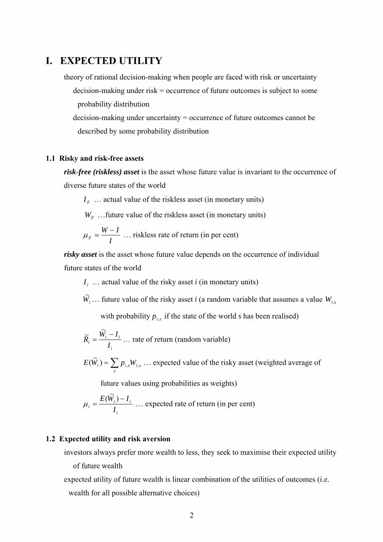
Utility function of a risk-averse investor

U

utility of expected value

expected utility

expected value

2W1W FWWE =)~(

4

expected value of risky investment = )~(WE

expected utility of risky investment = )()()]~([ 2211 WUpWUpWUE +=

utility of the expected value of risky investment = )())~(( 2211 WpWpUWEU +=

risk aversion

investor with aversion to risk prefers the expected value of a risky investment for sure to

the risky investment itself

)]~([)]~([ WUEWEU >

aversion to risk is the consequence of declining marginal utility function ( 0)(' <WU )

expected utility of risky asset = )()()]~([ 2211 WUpWUpWUE += <

))~(()( 2211 WEUWpWpU =+ = utility of expected value

a person who prefers the gamble is a risk lover (he has an increasing marginal utility

function)

a person who is indifferent is risk neutral (he has a constant marginal utility function)

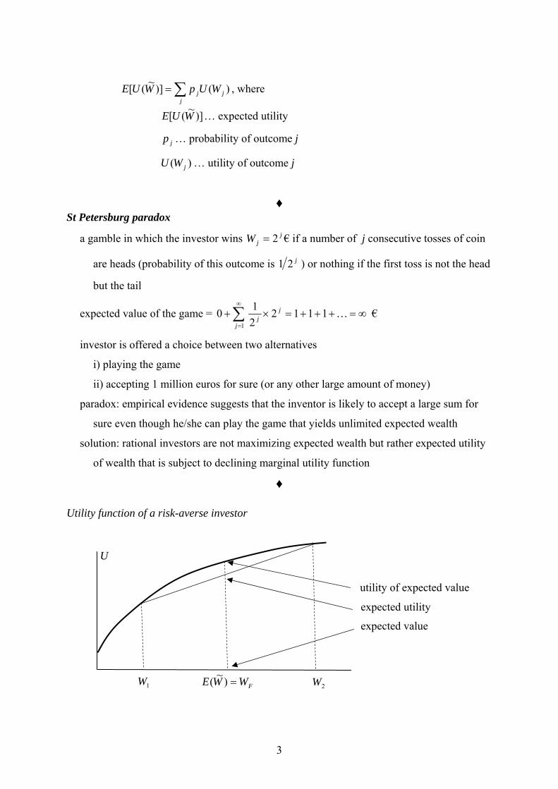
measures of risk aversion

absolute risk premium is the maximum amount of wealth an individual would be willing

to give up in order to avoid the risky investment

))~(()]~([ AWEUWUE π−=

certainty equivalent of the risky investment (CE) is the level of wealth that individual

would accept with certainty if the risky investment was removed

Measurement of risk premium

U

2W1W )~(WE

)]~([ WUE

Aπ

)~(CE W

5

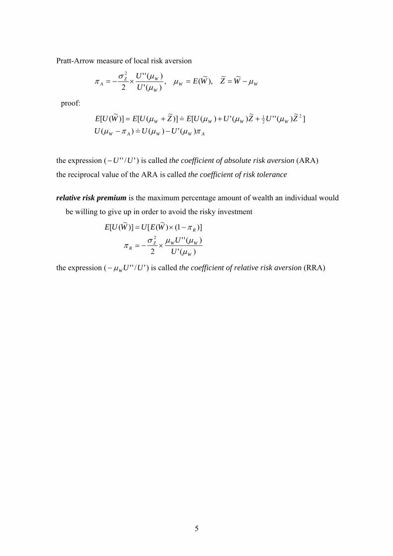
Pratt-Arrow measure of local risk aversion

WWW

WZA WZWE

UU

µµµµσ

π −==×−= ~~),~(,)(')(''

2

2

proof:

AWWAW

WWWW

UUUZUZUUEZUEWUE

πµµπµµµµµ

)(')()(]~)(''~)(')([)]~([)]~([ 2

21

−=−

++=+=

&

&

the expression ( '/'' UU− ) is called the coefficient of absolute risk aversion (ARA)

the reciprocal value of the ARA is called the coefficient of risk tolerance

relative risk premium is the maximum percentage amount of wealth an individual would

be willing to give up in order to avoid the risky investment

)('

)(''2

)]1()~([)]~([2

W

WWZR

R

UU

WEUWUE

µµµσ

π

π

×−=

−×=

the expression ( '/'' UUWµ− ) is called the coefficient of relative risk aversion (RRA)

6

II. DECISION-MAKING IN THE RISK-RETURN SPACE utility functions are not directly observable that raises demand for a more practical

approach

decision-making in risky environment is thus conventionally designed in the framework of

two variables: - the asset’s return (expected rate of risky returns)

- the asset’s risk (variability or volatility of risky returns)

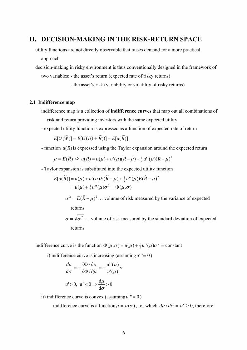
2.1 Indifference map

indifference map is a collection of indifference curves that map out all combinations of

risk and return providing investors with the same expected utility

- expected utility function is expressed as a function of expected rate of return

)]~([))]~1(([)]~([ RuERIUEWUE =+=

- function )(Ru is expressed using the Taylor expansion around the expected return

)~(RE=µ 221 ))((''))((')()( µµµµµ −+−+= RuRuuRu

- Taylor expansion is substituted into the expected utility function

),()('')(

)~()('')~()(')()]~([2

21

221

σµσµµ

µµµµµ

Φ=+=

−+−+=

uu

REuREuuRuE

22 )~( µσ −= RE … volume of risk measured by the variance of expected

returns

2σσ = … volume of risk measured by the standard deviation of expected

returns

indifference curve is the function constant)('')(),( 221 =+=Φ σµµσµ uu

i) indifference curve is increasing (assuming 0''' =u )

σµµ

µσ

σµ

)(')(''

//

uu

dd

−=∂Φ∂∂Φ∂

−=

0 dd 0 u´´ 0, ' >⇒<>σµu

ii) indifference curve is convex (assuming 0''' =u )

indifference curve is a function )(σµµ = , for which '/ µσµ =dd > 0, therefore

7

0)'(

')''(')''''''()(')(''

2

2

>−+

=⎟⎟⎠

⎞⎜⎜⎝

⎛−=⎟

⎠⎞

⎜⎝⎛

uuuuu

uu

dd

dd

dd σµσµσ

µµ

σσµ

σ

Indifference map in the risk-return space

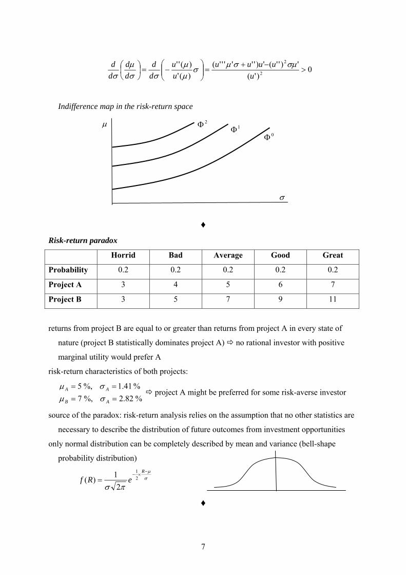
♦ Risk-return paradox

Horrid Bad Average Good Great

Probability 0.2 0.2 0.2 0.2 0.2

Project A 3 4 5 6 7

Project B 3 5 7 9 11

returns from project B are equal to or greater than returns from project A in every state of

nature (project B statistically dominates project A) no rational investor with positive

marginal utility would prefer A

risk-return characteristics of both projects:

%82.2%,7%41.1%,5

====

AB

AA

σµσµ

project A might be preferred for some risk-averse investor

source of the paradox: risk-return analysis relies on the assumption that no other statistics are

necessary to describe the distribution of future outcomes from investment opportunities

only normal distribution can be completely described by mean and variance (bell-shape

probability distribution)

σµ

πσ

−×−

=R

eRf 21

21)(

♦

µ

σ

0Φ0

2Φ0

1Φ0

8

2.2 Compendium of risk-return calculus

a) one risky asset

iR~ … rate of return of a risky asset i (random variable subject to a normal probability

distribution of future outcomes)

)~( ii RE=µ … expected return of risky asset i

22 )~( iii RE µσ −= …risk (volatility) of risky asset i measured by variance

2σσ =i … risk (volatility) of risky asset i measured by standard deviation

b) portfolio of risky assets

N … number of assets in a portfolio

iθ … percentage representation of the asset i in the portfolio

∑=

=N

iiiP RR

1

~~ θ … rate of return of portfolio P (random variable)

∑=

==N

iiiPP RE

1)~( µθµ … expected rate of return of portfolio P

[ ]

∑ ∑∑

∑ ∑∑∑∑

∑

= +==

= +=== =

=

+=

+=⎥⎦

⎤⎢⎣

⎡−−=

⎥⎦

⎤⎢⎣

⎡−=−=

N

i

N

ijijjiji

N

iii

N

i

N

ijijji

N

iii

N

i

N

jjjiiji

N

iiiiPPP

RRE

RERE

1 11

22

1 11

22

1 1

2

1

22

2

2)~)(~(

)~()~(

ρσσθθσθ

σθθσθµµθθ

µθµσ

[ ]

[ ] ∑∑

∑

==

=

=−−=

⎥⎦

⎤⎢⎣

⎡−−=−−=

N

iiPi

N

iiiPPi

N

iiiiPPPPPPP

RRE

RRERRE

11

1

2

)~)(~(

)~()~()~)(~(

σθµµθ

µθµµµσ

2Pσ … risk (volatility) of portfolio P (measured by variance)

ijσ …. covariance between rates of return of asset i and j

ijjijjiiij RRE ρσσµµσ =−−= )]~)(~[(

iPσ …. covariance between rates of return asset i and portfolio P

9

[ ]

∑

∑∑

=

==

=

−−=⎥⎦

⎤⎢⎣

⎡−−=

N

jijj

N

jjjiij

N

jjjjiiiP RRERRE

1

11)~)(~()~()~(

σθ

µµθµθµσ

ijρ … correlation coefficient between rates of return of assets i and j

11, ≤≤−= ijji

ijij ρ

σσσ

ρ

♦ A portfolio is composed of two risky assets with following features:

%.60

%,60%,50%,16%,40%,75%,20

12

222

111

−=======

ρθσµθσµ

We get

%27268.0072.0

072.06.05.075.06.04.025.06.075.04.0

%6.1716.06.02.04.022222

===

=×××××−×+×=

=×+×=

P

P

P

σ

σ

µ

manifestation of the diversification effect: by combining risky assets one can achieve a

portfolio with a lower risk than are the risks of the assets of which the portfolio is

composed

♦

c) matrix notation

volatility matrix V:

⎥⎥⎥

⎦

⎤

⎢⎢⎢

⎣

⎡=

3

2

1

000000

σσ

σV

correlation matrix C:

⎥⎥⎥

⎦

⎤

⎢⎢⎢

⎣

⎡=

11

1

2313

2312

1312

ρρρρρρ

C

variance-covariance matrix VCV:

10

VCVVCV ××=⎥⎥⎥

⎦

⎤

⎢⎢⎢

⎣

⎡

=232313

232212

131221

σσσσσσσσσ

weighting matrix W:

[ ]321 θθθ=W

portfolio risk 2Pσ :

')(2 WVCVWP ××=σ

2.3 Investment opportunity set

investment opportunity set (frontier) shows the risk-return trade-offs available to investors

that are offered by various combinations of risky assets in a portfolio

a) perfectly correlated assets ( 112 =ρ )

22112

2211

212122

22

21

21

2211

)(

12

σθσθσθσθ

σσθθσθσθσ

µθµθµ

+=+=

×++=

+=

P

P

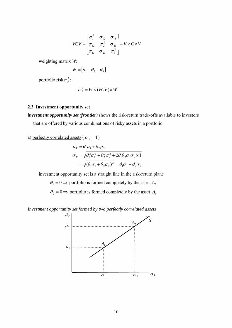
investment opportunity set is a straight line in the risk-return plane

⇒= 01θ portfolio is formed completely by the asset 2A

⇒= 02θ portfolio is formed completely by the asset 1A

Investment opportunity set formed by two perfectly correlated assets

Pµ

2µ

1µ

1σ 2σ Pσ

1A

2A S

11

♦ If the returns of the two assets from the previous example are perfectly correlated, a resulting

portfolio that preserves the assets’ weights (40 % and 60 %) will have following features:

%605.06.075.04.0

%6.1716.06.02.04.0=×+×==×+×=

P

P

σµ

Diversification effect is absent.

♦

short-selling beyond the segment 21 AA means that an investor borrows one of the assets and

uses proceeds from its sale for buying the other asset

short-selling is advantageous strategy if

i) a stock price is expected to decline in the future

ii) the stock price is expected to rise but there is another stock in a portfolio with a

higher realised return

clarification of negative weights in case of short-selling

i) short selling is not available

- the initial amount I has been invested into the two assets of a portfolio

21 III += , ,II i

i =θ for i = 1, 2.

- the assets generate rates of return

i

iii I

IWR

−= for i = 1, 2.

- rate of return of the portfolio can be expressed as a weighted average of individual

returns

( ) ( )

22112

222

1

1112121 RRI

IWII

IIW

II

IIIWW

IIWRP θθ +=

−×+

−×=

+−+=

−=

both weights are positive: 10 and 10 21 ≤≤≤≤ θθ

ii) short selling is available

- a borrowed amount 1I of the first asset is sold and proceeds from sale are invested

into the second asset, therefore

12 III +=

12

- a part of the return from the second asset must be used for buying back the

borrowed amount of the first asset, therefore

12 WWW −=

- rate of return of the portfolio is expressed as a weighted average of individual

returns

( ) ( )2211

222

1

1111212 RRI

IWII

IIW

II

IIIWW

IIWRP θθ +=

−×+

−×−=

−−−=

−=

some weights are negative: 1 and 0 21 ≥≤ θθ

b) perfectly inversely correlated assets ( 112 −=ρ )

22112

2211

212122

22

21

21

2211

)(

2

σθσθσθσθ

σσθθσθσθσ

µθµθµ

−=−=

−+=

+=

P

P

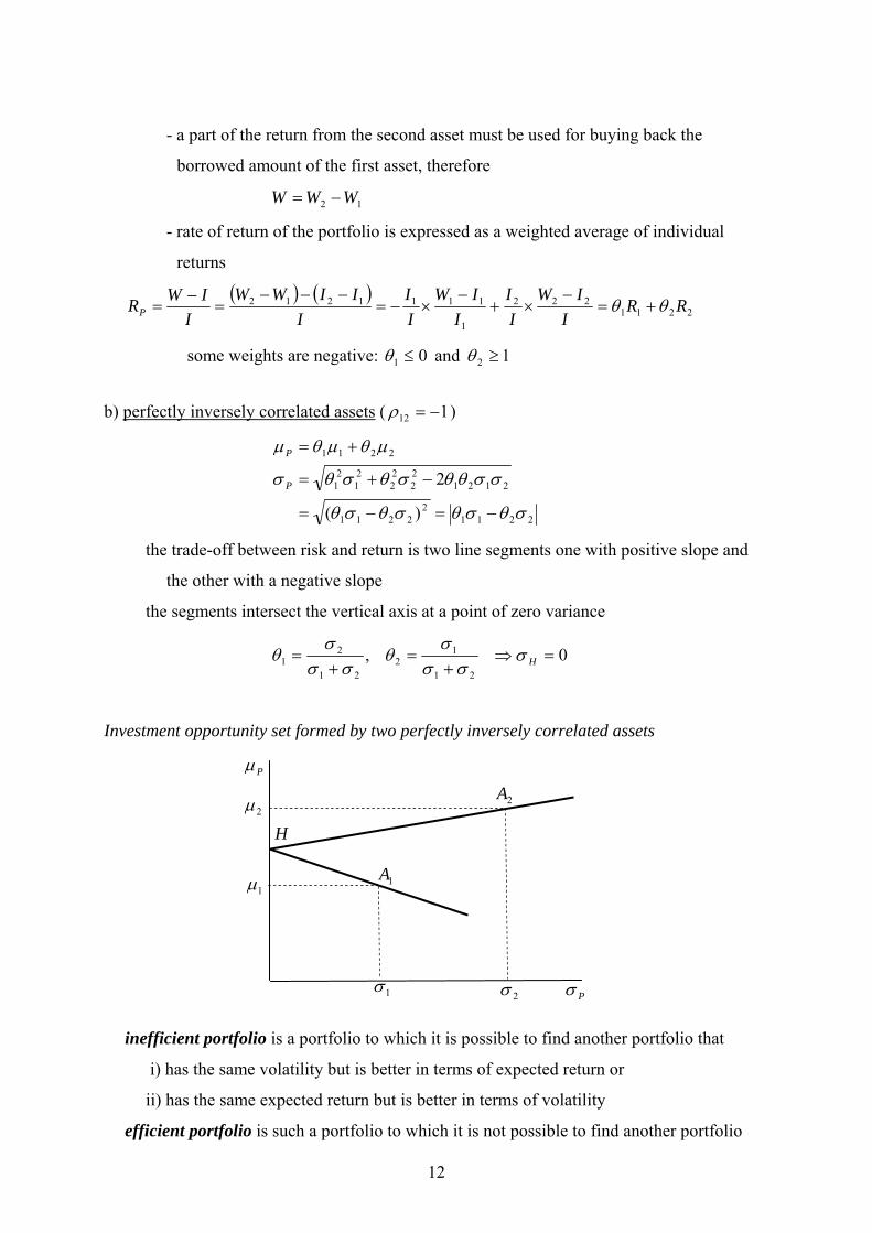
the trade-off between risk and return is two line segments one with positive slope and

the other with a negative slope

the segments intersect the vertical axis at a point of zero variance

0,21

12

21

21 =⇒

+=

+= Hσ

σσσ

θσσ

σθ

Investment opportunity set formed by two perfectly inversely correlated assets

inefficient portfolio is a portfolio to which it is possible to find another portfolio that

i) has the same volatility but is better in terms of expected return or

ii) has the same expected return but is better in terms of volatility

efficient portfolio is such a portfolio to which it is not possible to find another portfolio

2µ

1µ

2σ Pσ

1A

2A

H

1σ

Pµ

13

that either is better in terms of expected return (for a given risk) or is better in terms of

risk (for a given expected return)

efficient investment opportunity set (frontier) is the set of all efficient portfolios

minimum risk portfolio is a portfolio with lowest variance among all available portfolios

♦

If the returns of the two assets from the previous example are perfectly inversely correlated, a

resulting portfolio that preserves the assets’ weights (40 % and 60 %) will have following

features:

%05.06.075.04.0

%6.1716.06.02.04.0=×−×=

=×+×=

P

P

σµ

Diversification effect is complete.

♦

c) uncorrelated assets ( 012 =ρ )

22

22

21

21

2211

σθσθσ

µθµθµ

+=

+=

P

P

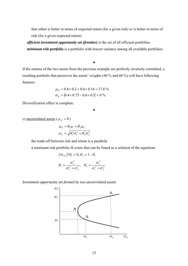
the trade-off between risk and return is a parabola

a minimum risk portfolio H exists that can be found as a solution of the equations

121 1,0 θθθσ −==∂∂ P

22

21

21

222

21

22

1 ,σσ

σθ

σσσ

θ+

=+

=

Investment opportunity set formed by two uncorrelated assets

2µ

1µ

1σ 2σ Pσ

1A

2A

H

Pµ

14

the opportunity set has the efficient part (the upper part of the parabola) and the

inefficient part (the lower part of the parabola)

♦

If the returns of the two assets from the previous example are uncorrelated, a resulting

portfolio that preserves the assets’ weights (40 % and 60 %) will have following features:

%425.06.075.04.0

%6.172222 =×+×=

=

P

P

σ

µ

The weights of a minimum risk portfolio are following:

%6931.01%,315.075.0

5.0222

2

1 =−==+

= θθ

♦

d) many risky assets

investment opportunity set is a collection of all risk-return pairs ),( PP µσ that

correspond to some structure of weights in a portfolio composed of a given number

of risky assets

∑∑

∑

= =

=

=

=

N

i

N

jijjijiP

N

iiiP

1 1

1

ρσσθθσ

µθµ

for all ∑=

=N

ii

1

1θ

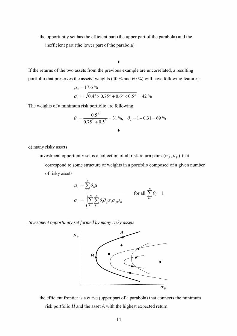
Investment opportunity set formed by many risky assets

the efficient frontier is a curve (upper part of a parabola) that connects the minimum

risk portfolio H and the asset A with the highest expected return

Pσ

Pµ A

H ••

•

••

••

•

•

15

all interior portfolios and all portfolios corresponding to a lower part of the parabola are

inefficient (dominated) portfolios

individual points of the investment opportunity set can be determined by solving

programming problems

Pσ → min subject to a given Pµ

Pµ → max subject to a given Pσ

e) one risk-free and one risky asset

AAAAP

AAFFP

σθσθσ

µθµθµ

==

+=22

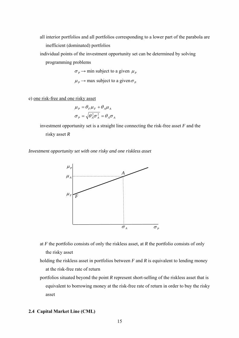
investment opportunity set is a straight line connecting the risk-free asset F and the

risky asset R

Investment opportunity set with one risky and one riskless asset

at F the portfolio consists of only the riskless asset, at R the portfolio consists of only

the risky asset

holding the riskless asset in portfolios between F and R is equivalent to lending money

at the risk-free rate of return

portfolios situated beyond the point R represent short-selling of the riskless asset that is

equivalent to borrowing money at the risk-free rate of return in order to buy the risky

asset

2.4 Capital Market Line (CML)

Pσ

Pµ

Fµ

Aσ

Aµ A

F

16

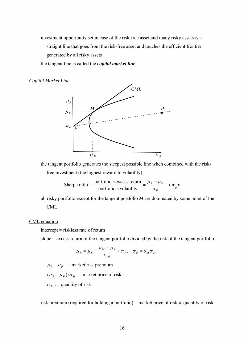
investment opportunity set in case of the risk-free asset and many risky assets is a

straight line that goes from the risk-free asset and touches the efficient frontier

generated by all risky assets

the tangent line is called the capital market line

Capital Market Line

the tangent portfolio generates the steepest possible line when combined with the risk-

free investment (the highest reward to volatility)

Sharpe ratio = P

P

FP maxvolatility sportfolio'

return excess sportfolio'→

−=

σµµ

all risky portfolio except for the tangent portfolio M are dominated by some point of the

CML

CML equation

intercept = riskless rate of return

slope = excess return of the tangent portfolio divided by the risk of the tangent portfolio

MMPPM

FMFP σθσσ

σµµ

µµ =×−

+= ,

FP µµ − … market risk premium

PFP σµµ )( − … market price of risk

Pσ … quantity of risk

risk premium (required for holding a portfolio) = market price of risk × quantity of risk

•Mµ

Fµ

M

F

P

CML

Mσ Pσ

Pµ

17

current fair price of a portfolio = riskfor adjusted ratediscount 1

valuefuture1

valuefuture+

=+ Pµ

♦ The tangent portfolio whose standard deviation is 30 % is expected to yield 18 %. The risk-

free return is estimated at 9 %. What is the appropriate rate of return on a portfolio consisting

of 20 % invested in the risk-free asset and 80 % invested in the tangent portfolio?

%24.03.08.0 =×=×= MMP σθσ

%2.1624.03.0

09.018.009.0 =×−

+=Pµ

The same answer is provided by the formula

%2.1618.08.009.02.0 =×+×=+= MMFFP µθµθµ

♦

computing the tangent portfolio

The task is to find the set of weights Nθθθ ,...,, 21 for which the Sharpe ratio is maximised

,max)(

ratio Sharpe,,

1,

1

1 NN

jiijji

N

iFii

P

FP

θθ

σθθ

µµθ

σµµ

K→

−=

−=Θ=

∑

∑

=

=

subject to .11∑=

=N

iiθ

First order conditions 0=∂Θ∂ iθ give a system of N linear equations for unknown

quantities iZ ,

22211

22221212

11222111

.....................................................................

............

NNNNFN

NNF

NNF

ZZZ

ZZZZZZ

σσσµµ

σσσµµσσσµµ

+++=−

+++=−+++=−

,

where

.

1∑=

= N

jj

ii

Z

Zθ

18

III. CAPITAL ASSET PRICING MODEL (CAPM) CAPM is the most important model for determining the market price of risk and the

appropriate measure of risk: the equilibrium rates of return on all risky assets are a

function of their covariance with the market portfolio

major contributors: William Sharpe (1964), Jack Treynor (1962), John Lintner (1965)

assumptions:

- all investors exhibit the aversion to risk

- investors can buy and sell all risky securities at equilibrium market prices (demand for

each security equals its supply)

- inventors can borrow or lend at the risk-free interest rate

- investors hold only efficient portfolios of traded securities

- investors have homogeneous expectations regarding volatilities, correlations and

expected returns (they perceive the same investment opportunity set)

- there are no taxes or other transactions costs

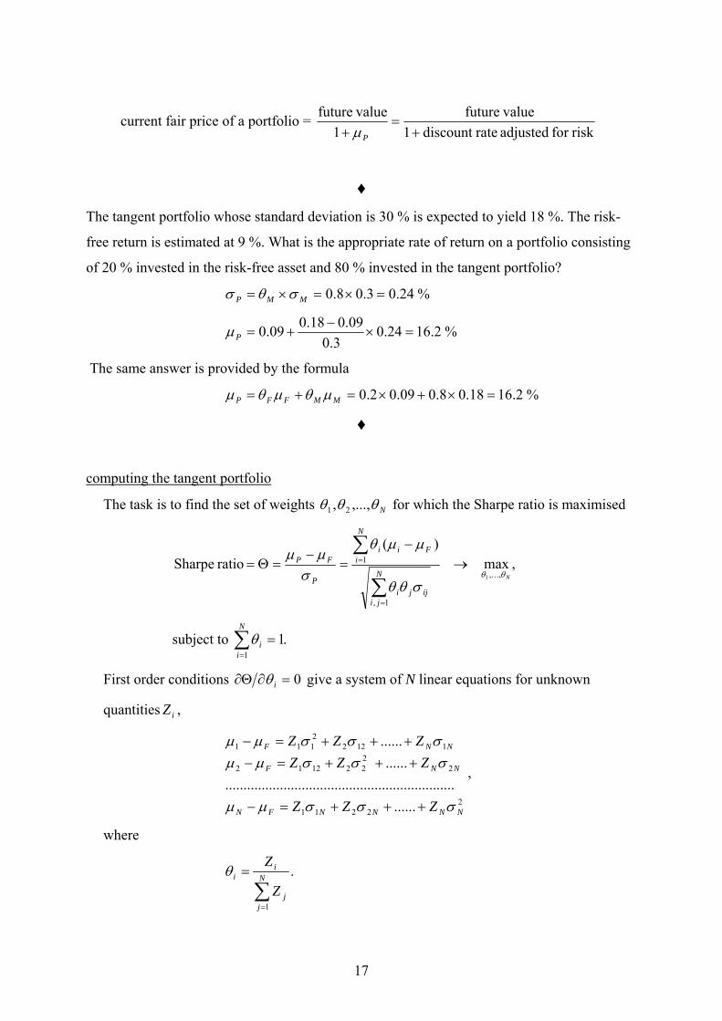
3.1 Market portfolio as a state of general equilibrium

two funds separation theorem

- portfolios of all investors consist of different combinations of only two assets:

a) the risk-free asset F and b) the tangent portfolio M

- all investors make selection only among portfolios that belong to the CML

- investors hold identical combinations of risky assets even though they have different

attitudes toward risk

Optimal choice of risk-averse investors

M

Pσ

Pµ

CML

F

19

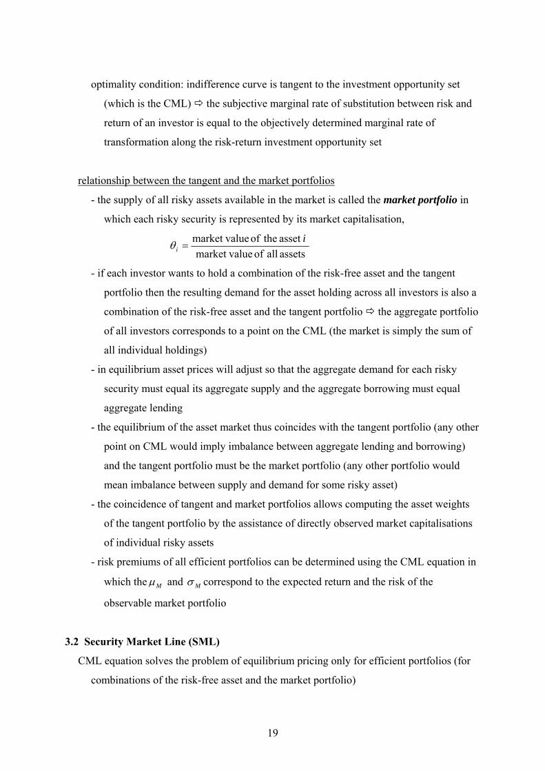
optimality condition: indifference curve is tangent to the investment opportunity set

(which is the CML) the subjective marginal rate of substitution between risk and

return of an investor is equal to the objectively determined marginal rate of

transformation along the risk-return investment opportunity set

relationship between the tangent and the market portfolios

- the supply of all risky assets available in the market is called the market portfolio in

which each risky security is represented by its market capitalisation,

assetsallofvaluemarket asset theof valuemarket i

i =θ

- if each investor wants to hold a combination of the risk-free asset and the tangent

portfolio then the resulting demand for the asset holding across all investors is also a

combination of the risk-free asset and the tangent portfolio the aggregate portfolio

of all investors corresponds to a point on the CML (the market is simply the sum of

all individual holdings)

- in equilibrium asset prices will adjust so that the aggregate demand for each risky

security must equal its aggregate supply and the aggregate borrowing must equal

aggregate lending

- the equilibrium of the asset market thus coincides with the tangent portfolio (any other

point on CML would imply imbalance between aggregate lending and borrowing)

and the tangent portfolio must be the market portfolio (any other portfolio would

mean imbalance between supply and demand for some risky asset)

- the coincidence of tangent and market portfolios allows computing the asset weights

of the tangent portfolio by the assistance of directly observed market capitalisations

of individual risky assets

- risk premiums of all efficient portfolios can be determined using the CML equation in

which the Mµ and Mσ correspond to the expected return and the risk of the

observable market portfolio

3.2 Security Market Line (SML)

CML equation solves the problem of equilibrium pricing only for efficient portfolios (for

combinations of the risk-free asset and the market portfolio)

20

CML: M

PFMFP σ

σµµµµ ×−+= )(

SML provides the general answer to equilibrium pricing for all risky assets or risky

portfolios

SML: PFMFM

PMFMFP βµµµ

σσ

µµµµ ×−+=×−+= )()( 2

PMσ …covariance between the risky and the market portfolio

Pβ … beta of the risky portfolio

beta of a security is the expected percentage change in the excess return of a security

for a 1 % change in the excess return of the market portfolio

)()(

FM

FPP µµ

µµβ

−∂−∂

=

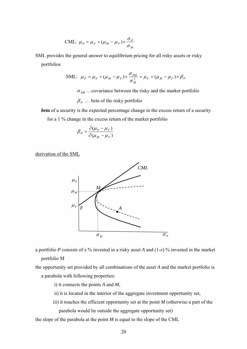
derivation of the SML

a portfolio P consists of x % invested in a risky asset A and (1-x) % invested in the market

portfolio M

the opportunity set provided by all combinations of the asset A and the market portfolio is

a parabola with following properties:

i) it connects the points A and M,

ii) it is located in the interior of the aggregate investment opportunity set,

iii) it touches the efficient opportunity set at the point M (otherwise a part of the

parabola would lie outside the aggregate opportunity set)

the slope of the parabola at the point M is equal to the slope of the CML

Mµ

Fµ

M

F

CML

Mσ Pσ

Pµ

•A

21

a) expected return and risk of the portfolio P

AMMAP

MAP

xxxx

xx

σσσσ

µµµ

)1(2)1(

)1(2222 −+−+=

−+=

b) risk-return trade-off secured by the portfolio P (slope of the tangent line for a given

x)

AMMA

AMMA

MA

P

P

P

P

xxxx

xxxdxddxd

dd

σσσ

σσσµµ

σµ

σµ

)1(2)1(2

)21(2)1(222222

22

−+−+

−+−−−

==

risk-return trade-off at the point that corresponds to the market portfolio (P = M)

2

20

2

220

M

AMM

MA

xP

P

ddx

σ

σσµµ

σµ

+−−

=⇒==

risk-return trade-off at the market portfolio is equal to the slope of CML

M

FM

M

AMM

MA

σµµ

σ

σσµµ −

=+−−

2

2

2

22

the last equation can be arranged into the formula called the security market line

2

2

,)(

)(

M

AMAAFMF

M

AMFMFA

σσ

ββµµµ

σσ

µµµµ

=×−+=

−+=

required rate of return from holding a risky asset is proportional to the beta of the asset

quantity of risk is measured by the covariance with the market beta and not by the

variance of the assets’ returns

Security market line

iβ

iµ

Fµ

Mµ M

F

SML

22

♦

Calculate the risk premium for a risky asset whose correlation with the market is 85 % and

standard deviation 35 %. The market portfolio has expected return 15 % and standard

deviation 20%. The risk-free rate of return is 5 %.

%9.142.035.085.0)05.015.0(

)()()( 2

=××−=

××−=×−=×−=−M

iiMFM

M

iMFMiFMFi σ

σρµµ

σσ

µµβµµµµ

♦

betas of specific assets:

riskless asset: 02 ==M

FMF σ

σβ

market portfolio: 12

2

2 ===M

M

M

MMM σ

σσσ

β

efficient portfolio (points on CML):

)~(Var])1(~[Var 2 MFM MMM θθθ =−+

)~(Var)~,~Cov[]~,)1(~Cov[ MMMMFM MMMM θθθθ ==−+

MM

MM

M

EME θ

σσθ

σσ

β === 2

2

2

for efficient portfolios the SML is identical to the CML

SML: MFMFEFMFE θµµµβµµµµ )()( −+=−+=

CML: MFMFM

EFMFE θµµµσσ

µµµµ )()( −+=−+=

beta of a portfolio is equal to the weighted average of betas of assets from which the

portfolio is composed:

∑∑ ==

−−Σ=−−Σ==

iii

i M

iMi

MMiiiM

MMiiiMM

PMP rrERRE

βθσσθ

µµθσ

µµθσσ

σβ

2

222 )]~)(~[(1)]~)(~([1

1=Mβ0=Fβ

23

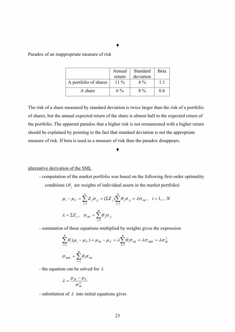
♦ Paradox of an inappropriate measure of risk

Annual return

Standard deviation

Beta

A portfolio of shares 11 % 4 % 1.1

A share 6 % 8 % 0.6

The risk of a share measured by standard deviation is twice larger than the risk of a portfolio

of shares, but the annual expected return of the share is almost half to the expected return of

the portfolio. The apparent paradox that a higher risk is not remunerated with a higher return

should be explained by pointing to the fact that standard deviation is not the appropriate

measure of risk. If beta is used as a measure of risk then the paradox disappears.

♦

alternative derivation of the SML

- computation of the market portfolio was based on the following first-order optimality

conditions ( jθ are weights of individual assets in the market portfolio)

NiZZ iMji

N

jjjji

N

jjFi K,1,)(

11==Σ==− ∑∑

==

λσσθσµµ

∑=

=Σ=M

jjijiMjZ

1, σθσλ

- summation of these equations multiplied by weights gives the expression

∑∑==

===−=−N

iMMMiMiFM

N

iFii

1

2

1)( λσλσσθλµµµµθ

∑=

=M

iiMiMM

1σθσ

- the equation can be solved for λ

2M

FM

σµµ

λ−

=

- substitution of λ into initial equations gives

24

iFMFiMM

FMFi βµµµσ

σµµ

µµ )(2 −+=−

+=

3.3 Portfolio diversification

diversification effect occurs whenever a growing number of assets combined in a

portfolio results in a lower risk of the portfolio

features of diversification:

- there is a limit of diversification and only some portion of total risk can be

diversified away

- if diversification effect can be achieved at zero cost (by simply adding more assets

in a portfolio) then the equilibrium market prices do not take account of the risk

that can be diversified away; investors are not compensated for holding

diversifiable risk

- the appropriate measure of risk for a single asset is its beta because this is the part

of the total risk that is correlated with the market portfolio and cannot be removed

by diversification

diversification effect in an equally weighted portfolio

N … number of assets

Ni /1=θ … the weight of the asset i in a portfolio

L …the largest individual asset variance ( Li ≤2σ )

σ … average covariance (the sum of all covariances is equal to σ×−× )1(NN )

σ

σσσθθσθσ

×−

×+××≤

≤+=+= ∑ ∑∑∑∑∑= +=== +==

2)1(2)(1

212

22

1 12

1

22

1 11

222

NNN

LNN

NN

N

i

N

ijij

N

ii

N

i

N

ijijji

N

iiiP

the variance term converges to zero this part of risk can be diversified away

the covariance term approaches the average covariance σ this part of risk cannot

be avoided

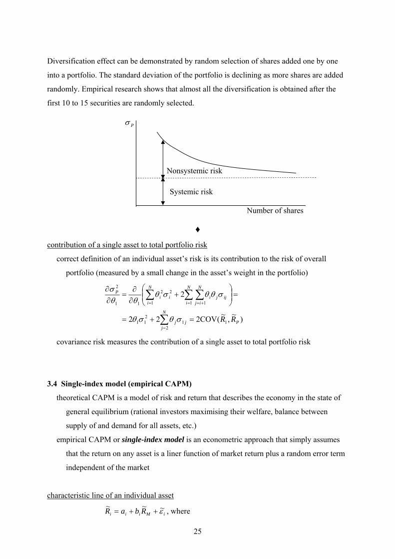
total risk = non-diversifiable (systemic, market) risk + diversifiable (nonsystemic, specific,

idiosyncratic, residual) risk

♦

25

Diversification effect can be demonstrated by random selection of shares added one by one

into a portfolio. The standard deviation of the portfolio is declining as more shares are added

randomly. Empirical research shows that almost all the diversification is obtained after the

first 10 to 15 securities are randomly selected.

♦ contribution of a single asset to total portfolio risk

correct definition of an individual asset’s risk is its contribution to the risk of overall

portfolio (measured by a small change in the asset’s weight in the portfolio)

)~,~(COV222

2

12

1211

1 11

22

11

2

P

N

jjj

N

i

N

ijijji

N

iii

P

RR=+=

=⎟⎟⎠

⎞⎜⎜⎝

⎛+

∂∂

=∂∂

∑

∑ ∑∑

=

= +==

σθσθ

σθθσθθθ

σ

covariance risk measures the contribution of a single asset to total portfolio risk

3.4 Single-index model (empirical CAPM)

theoretical CAPM is a model of risk and return that describes the economy in the state of

general equilibrium (rational investors maximising their welfare, balance between

supply of and demand for all assets, etc.)

empirical CAPM or single-index model is an econometric approach that simply assumes

that the return on any asset is a liner function of market return plus a random error term

independent of the market

characteristic line of an individual asset

iMiii RbaR ε~~~ ++= , where

Number of shares

Systemic risk

Nonsystemic risk

Pσ

26

iR~ … expected return on the asset i

MR~ … expected return on the selected market index (fundamental factor)

ia … risk-free component of the return

ib … sensitivity of the return on the asset i to a change in the market return

iε~ …random error term subject to following properties

0)~,~cov(,0)~,~cov(,)(,0)~( 22 ==== jiMiiii REE εεεηεε

expected rate of return, risk an covariance of an individual asset

Mii

MiiiMiii

baERbEaERbaE

µεεµ

+=++=++= )~()~()()~~(

222

222

222

)(]~)~[(2)~(

]~)~([)]()~~[(

iMi

iiMMiMMi

iMMiMiiiMiii

b

EREbREb

RbEbaRbaE

ησ

εεµµ

εµµεσ

+=

+−+−=

+−=+−++=

= systemic risk + non-systemic risk

2

)]~)~()(~)~([()]~)(~[(

Mji

jMMjiMMijjiiij

bb

RbRbERRE

σ

εµεµµµσ

=

+−+−=−−=

return and risk of a portfolio

MPP

M

iiiM

N

iiiP

N

i

N

i

N

iPMPPiiiiMii

N

iiiP

bcba

RbabRaRR

µθµθµ

εεθθθθ

+=+=

++=++==

∑∑

∑ ∑ ∑∑

==

= = ==

11

1 1 11

~~~~~~

2

2

222

1

22

1 1

2

1

222

1 11

222

PMP

N

iii

N

i

N

ijjijiM

N

iiiM

N

i

N

ijijji

N

iiiP

b

bbb

ησ

ηθθθσθσ

σθθσθσ

ε

+=

++=

+=

∑∑ ∑∑

∑∑∑

== +==

= +==

total risk of a portfolio is partitioned into systemic risk and non-systemic risk

requirements on a number of estimated variables:

variance-covariance approach: N variances 2iσ + )1(2

1 −NN covariances ijσ

27

50 shares ⇒ 1275 estimates

200 shares ⇒ 20100 estimates

single-index model: N coefficients β + N residual risks iη + market risk Mσ

50 shares ⇒101 estimates, 200 shares ⇒ 401 estimates

estimation of historical betas

linear regression is the statistical technique that identifies the best fitting line through a

set of points (standard least squares approach)

∑ →−++= min)(, 2,,, itittMiiti RRbaR µε

the formula for computing the regression coefficient ib is identical with the beta

derived in the CAMP beta is the slope of the regression line and is called

historical beta

iM

iM

tM

tMtii R

RRb β

σσ

=== 2,

,,

)VAR(),(COV

historical beta is estimated on historical data while a “true beta” depends on future

correlations and volatilities

♦ The variance (the total risk) of a portfolio is 35 %, the variance of the market portfolio is 25

% and the covariance between the two assets is 0.22.

systemic risk = 194.025.0

22.0)(

22

22

222 ==×= M

M

iMMi σ

σσ

σβ

nonsystemic risk = 156.0194.035.0 =−

correlation coefficient = %74.025.035.

22.0=

×=

Ml

iM

σσσ

The systemic part of the total risk of the portfolio amounts to 55 % ( )035/194.055.0 = and

therefore the residual 45 % must be attributed to nonsystemic risk.

♦

estimation of fundamental betas

fundamental beta is the output of the regression analysis in which the beta is made

28

dependent on a number of selected characteristics of a firm: dividend yield, volume

and growth of production, size of a firm, indebtedness, etc.

the forecast of the beta is based on forecasts of selected characteristics

the approach is based on the assumption of constant sensitivities of betas with respect to

chosen characteristics of a firm

29

IV. EXTENSIONS OF CAPM

4.1 No riskless asset

conclusion: the SML of the CAPM is still valid except that the rate of return on the risk-

free asset has been replaced by the expected rate of return on the so called zero-beta

portfolio

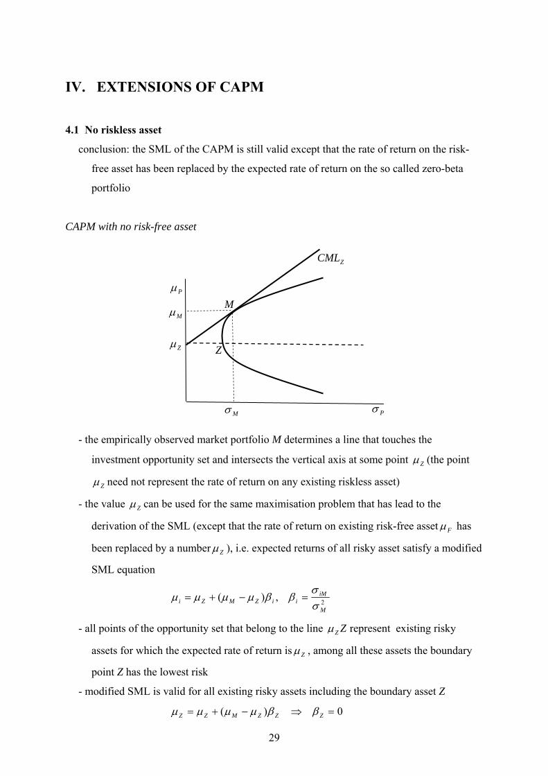
CAPM with no risk-free asset

- the empirically observed market portfolio M determines a line that touches the

investment opportunity set and intersects the vertical axis at some point Zµ (the point

Zµ need not represent the rate of return on any existing riskless asset)

- the value Zµ can be used for the same maximisation problem that has lead to the

derivation of the SML (except that the rate of return on existing risk-free asset Fµ has

been replaced by a number Zµ ), i.e. expected returns of all risky asset satisfy a modified

SML equation

2,)(M

iMiiZMZi σ

σββµµµµ =−+=

- all points of the opportunity set that belong to the line ZZµ represent existing risky

assets for which the expected rate of return is Zµ , among all these assets the boundary

point Z has the lowest risk

- modified SML is valid for all existing risky assets including the boundary asset Z

0)( =⇒−+= ZZZMZZ ββµµµµ

Z

Mµ

Zµ

M

Mσ Pσ

Pµ

ZCML

30

the asset Z (as all other assets belonging to the line ZZµ ) has zero beta, in other

words zero covariance with the market portfolio M

- the SML as the key upshot of the CAPM can still be preserved under assumption that the

rate of return on the risk-free asset can be substituted for the minimum variance zero

beta portfolio

practical limitations:

the modified CAPM relies heavily on the assumption that there are no constraints on

short sales

otherwise it makes virtually impossible to construct a zero-beta portfolio in a world

where almost all asset returns are positively correlated with the market

short selling allows making positive returns when the asset prices fall

Roll’s critique

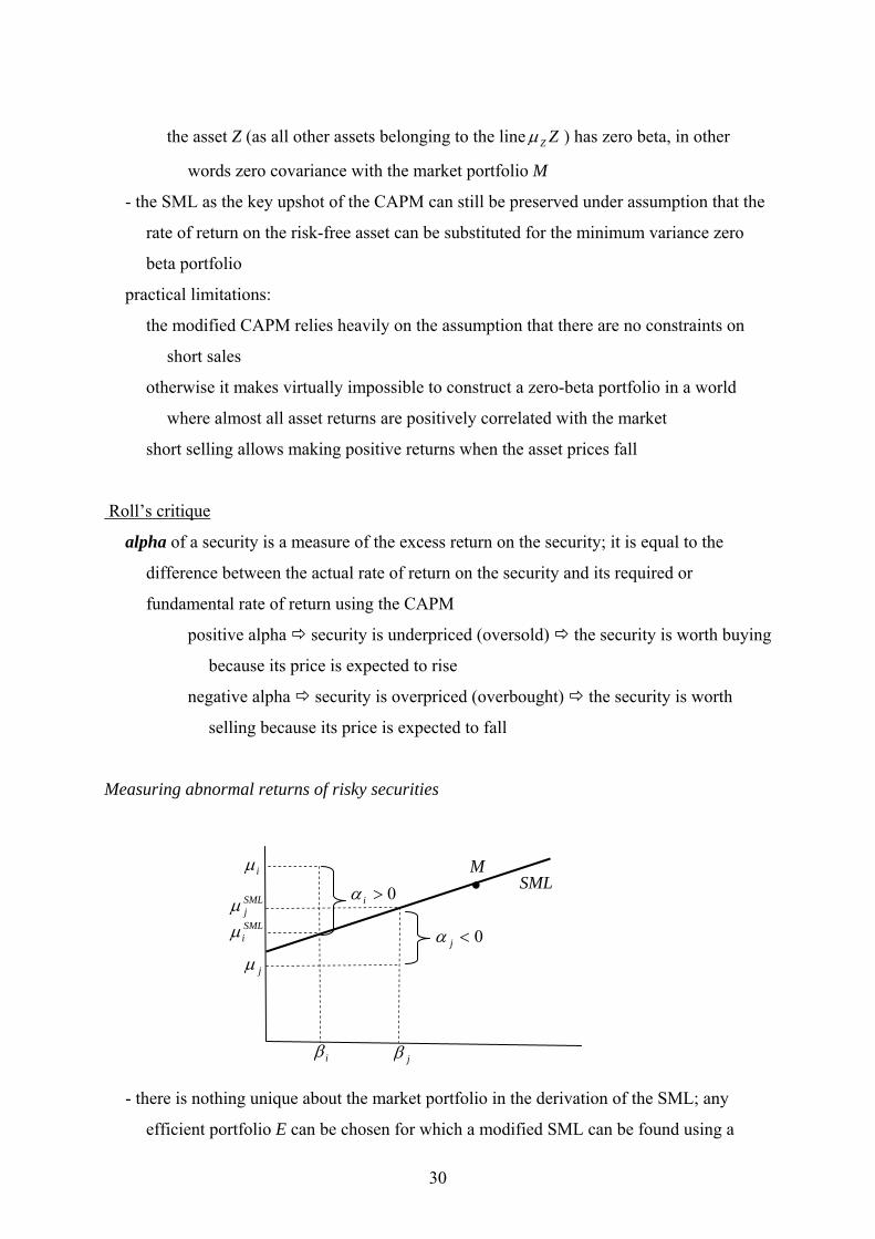
alpha of a security is a measure of the excess return on the security; it is equal to the

difference between the actual rate of return on the security and its required or

fundamental rate of return using the CAPM

positive alpha security is underpriced (oversold) the security is worth buying

because its price is expected to rise

negative alpha security is overpriced (overbought) the security is worth

selling because its price is expected to fall

Measuring abnormal returns of risky securities

- there is nothing unique about the market portfolio in the derivation of the SML; any

efficient portfolio E can be chosen for which a modified SML can be found using a

iµ

iβ

0<jα

SML •M

jµ

jβ

SMLjµ SMLiµ

0>iα

31

minimum variance portfolio Z that is uncorrelated with the selected efficient index

2,)(E

iEEi

Ei

EZE

EZ

Ei σ

σββµµµµ =−+=

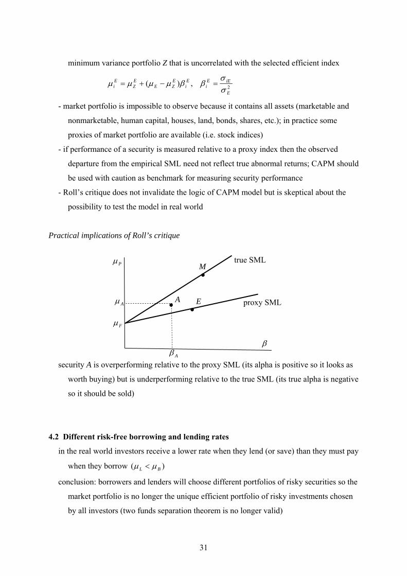
- market portfolio is impossible to observe because it contains all assets (marketable and

nonmarketable, human capital, houses, land, bonds, shares, etc.); in practice some

proxies of market portfolio are available (i.e. stock indices)

- if performance of a security is measured relative to a proxy index then the observed

departure from the empirical SML need not reflect true abnormal returns; CAPM should

be used with caution as benchmark for measuring security performance

- Roll’s critique does not invalidate the logic of CAPM model but is skeptical about the

possibility to test the model in real world

Practical implications of Roll’s critique

security A is overperforming relative to the proxy SML (its alpha is positive so it looks as

worth buying) but is underperforming relative to the true SML (its true alpha is negative

so it should be sold)

4.2 Different risk-free borrowing and lending rates

in the real world investors receive a lower rate when they lend (or save) than they must pay

when they borrow )( BL µµ <

conclusion: borrowers and lenders will choose different portfolios of risky securities so the

market portfolio is no longer the unique efficient portfolio of risky investments chosen

by all investors (two funds separation theorem is no longer valid)

Aµ

Aβ

true SMLM

Fµ

proxy SML

•

•E

β

Pµ

• A

32

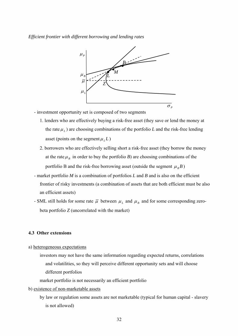
Efficient frontier with different borrowing and lending rates

- investment opportunity set is composed of two segments

1. lenders who are effectively buying a risk-free asset (they save or lend the money at

the rate Lµ ) are choosing combinations of the portfolio L and the risk-free lending

asset (points on the segment LLµ )

2. borrowers who are effectively selling short a risk-free asset (they borrow the money

at the rate Bµ in order to buy the portfolio B) are choosing combinations of the

portfolio B and the risk-free borrowing asset (outside the segment BBµ )

- market portfolio M is a combination of portfolios L and B and is also on the efficient

frontier of risky investments (a combination of assets that are both efficient must be also

an efficient assets)

- SML still holds for some rate µ between Lµ and Bµ and for some corresponding zero-

beta portfolio Z (uncorrelated with the market)

4.3 Other extensions

a) heterogeneous expectations

investors may not have the same information regarding expected returns, correlations

and volatilities, so they will perceive different opportunity sets and will choose

different portfolios

market portfolio is not necessarily an efficient portfolio

b) existence of non-marketable assets

by law or regulation some assets are not marketable (typical for human capital - slavery

is not allowed)

Pσ

Pµ

Lµ

L

B

M Bµ

•• •

µ Z

33

all assets are not perfectly divisible and traded at market that violates some of the

assumptions of two funds separation theorem

c) returns not normally distributed

if returns are normally distributed then only two parameters – mean and variance - are

needed to completely describe the probability distribution

practical obstacles to normal distribution:

- limited liability the largest negative return possible is minus 100 %

- empirical research shows that returns may have “fat tails” and no finite variance

d) other generalisations

inclusion of taxes, multi-period setting, monopoly power of some investors and

other relaxations of restrictive assumptions

4.4 Arbitrage Pricing Theory (APT)

formulated by Ross (1976)

assumptions

- no arbitrage condition: all assets that are using no wealth and have no risk must earn

zero return on average (perfectly competitive and frictionless capital markets)

- rate of return on any assets is a linear function of fundamental factors whose number is

much smaller than the number of risky assets (no special role for the market

portfolio)

iiiii FbFbaR ε+++= 2211~~~

kF~ ... the fundamental factor k common to the returns of all assets

0)~( =kFE

ikb … sensitivity of returns (factor loading) of the asset i to the factor k

ia … fixed component of the expected return

iε~ … random noise term in the returns on the asset i

)~,~(COV,0)~,~(COV,0)~( jikii FE εεεε ==

34

derivation of the APT formula

- a rate of return on a portfolio containing all risky assets

PPPP

N

iii

N

iii

N

i

N

i

N

iiiiiiiP

FbFba

bFbFaRR

ε

εθθθθθ

~~~

~~~~~

2211

1122

1 1 111

+++=

+++== ∑∑∑ ∑ ∑=== = =

- the portfolio can be adjusted in such a way that eliminates all systemic and unsystemic

risk

new weights of assets: iii δθθ +=′

very small changes in weights: Ni1

±≈δ

no additional wealth: 01

=∑=

N

iiδ

additional portfolio return:

i

N

iii

N

iii

N

iii

N

iii

N

iiP bFbFaRR εδδδδδ ~~~~~

12

121

11

11∑∑∑∑∑=====

+++==∆

- elimination of unsystemic risk = a weighted average of independent error terms will

approach zero in limit as N becomes large

0~1~11

→±≈ ∑∑==

N

ii

N

iii N

εεδ

- elimination of systemic risk = by an appropriate rebalancing the weighted average of

the systemic risk components for each factor can be made equal to zero (a number of

assets N exceeds substantially a number of factors)

∑∑==

==N

iii

N

iii bb

11

11 0,0 δδ

- the resulting change in the portfolio return after rebalancing

i

N

iiP aR ∑

=

=∆1

~ δ

- the accomplished change in a portfolio has no risk and requires no new wealth,

therefore it should yield the zero change in the expected rate of return

0)~()~(11

===∆=∆ ∑∑==

i

N

iii

N

iiPP RERE µδδµ

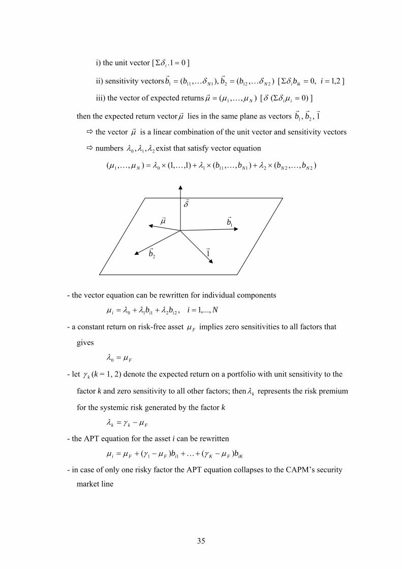
- statement in linear algebra

if vector ),( 1 Nδδδ Kr= is orthogonal to

35

i) the unit vector [ 01. =Σ iδ ]

ii) sensitivity vectors ),(),,( 21221111 NN bbbb δδ Kr

Kr

== [ 2,1,0 ==Σ ibikiδ ]

iii) the vector of expected returns ),,( 1 Nµµµ Kr= [ )0( =Σ iiµδδ ]

then the expected return vectorµr lies in the same plane as vectors 1,, 21

rrrbb

the vector µr is a linear combination of the unit vector and sensitivity vectors

numbers 210 ,, λλλ exist that satisfy vector equation

),,(),,()1,,1(),,( 222111101 NNNN bbbb KKKK ×+×+×= λλλµµ

- the vector equation can be rewritten for individual components

Nibb iii ,...,1,22110 =++= λλλµ

- a constant return on risk-free asset Fµ implies zero sensitivities to all factors that

gives

Fµλ =0

- let kγ (k = 1, 2) denote the expected return on a portfolio with unit sensitivity to the

factor k and zero sensitivity to all other factors; then kλ represents the risk premium

for the systemic risk generated by the factor k

Fkk µγλ −=

- the APT equation for the asset i can be rewritten

iKFKiFFi bb )()( 11 µγµγµµ −++−+= K

- in case of only one risky factor the APT equation collapses to the CAPM’s security

market line

1br

2br

µr

1r

δr

36

empirical estimates of APT

step 1: selection of common fundamental factors kF~ (k = 1, …, K) that are supposed to

influence expected returns on risky assets (i.e. inflation, dividend yield, firm’s size

and others)

step 2: on a given set of observations ),,,( 1 Kttit FFR K , t = 1,…, T, linear regression is

used to estimate sensitivities ikb that fit the equations

itKtiKtiiit FbFbaR ε++++= K11 , for a given i (i = 1, 2, …, N)

)~(VAR)~,~COV(

k

kiik F

FRb =

step 3: on a given set of estimated numbers ),,,( 1 iKii bb Kµ , i = 1,…,N, linear

regression is used to derive coefficients kλ that fit the equation

iiKKii bb ελλλµ ++++= K110