Portfolio strategies and performance

Journal of Financial Economics 5 (1977) 201-218. 0 North-Holland Publishing Company

PORTFOLIO STRATEGIES AND PERFORMANCE

Ted BLOOMFIELD, Richard LEFTWICH and John B. LONG, Jr.*

Graduate School of Management, University of Rochester, Rochester, NY 14627, U.S.A.

Received July 1977, revised version received August 1977

The relative performance of several portfolio selection strategies is assessed empirically. These strategies vary in sophistication from a ‘naive’ strategy of maintaining equal dollar investments in each stock available to a strategy that periodically uses updated parameter estimates to calculate new optimal proportions of portfolio value to be invested in the stocks available. Although it is to be expected a priori that relatively sophisticated strategies will perform at least as well as the more naive strategies, implementation costs will clearly differ across strategies and across investor-specific parameters such as total portfolio value. Thus estimation of the various strategies’ performance gross of these costs is a necessary consideration in rational strategy selection by any given investor.

1. Introduction

Since the seminal work of Markowitz’ almost 25 years ago, theoretical and empirical studies of optimal portfolio choice’ have defined optimality in terms of mean-variance efficiency. If an investor can borrow and lend at a ‘riskless’ rate of interest in addition to investing in risky securities, this characterization of portfolio choice takes a particularly simple form. Mean-variance efficiency is attained in this case by combining riskless borrowing or lending with an investment in the ‘tangency portfolio’ of risky securities - that portfolio whose expected rate of return in excess of the riskless rate is greatest as a fraction of the standard deviation of its rate of return, i.e., the portfolio with the maximum ‘reward-to-variability’ ratio. If there were no transaction costs and if investors had identical expectations, market equilibrium theory predicts that the relative dollar quantities (‘weights’) of individual stocks in the tangency portfolio would be proportional to the stocks’ total values and thus these weights would be trivial to compute.

*We wish to thank the referee, Eugene Fama, and Michael C. Jensen for their helpful comments.

‘See Markowitz (1952, 1956,1959). ‘See, for example, Johnson and Shannon (1974, 1973, Blume (1970). Evans (1970), Cohen

and Pogue (1967), Sharpe (1967), and Tobin (1958).

202 T. Bloomfield et al., Portfolio strategies and performance

Actual implementation of portfolio startegies designed to maximize the reward-to-variability ratio does involve non-negligible transaction costs which increase with the number of different stocks in the portfolio. This provides an incentive to restrict the set of stocks from which a tangency portfolio is chosen. Restricting portfolio size, however, involves not only a potential efficiency loss, but also non-trivial costs of computing portfolio weights. Market equilibrium theory does not offer the simple solution here that it does in the case of no transaction costs. Even if transaction costs are ignored, equilibrium theory does not imply that the tangency portfolio associated with a restricted set of stocks con- sists of those stocks held in proportion to their market values. The tangency portfolio weights mut be estimated and that estimation is both costly and subject to error.3 There is, however, a trade-off between estimation costs and estimation accuracy. Thus, in addition to restrictions on portfolio size, two other potential cost reduction techniques are (a) using cruder and less expensive estimation procedures and (b) reducing the frequency of incorporating ‘new’ data into portfolio weight estimates. The magnitude of the gross efficiency losses associated with use of any of these techniques is an empirical question.

In this paper, we empirically assess the performance (before transaction and estimation costs) of five different portfolio strategies that employ one or more of the cost reduction techniques mentioned above. With one exception, these strategies are all designed to approximate continuous investment in the tangency portfolio for the universe of stocks to which the strategies are applied. Using monthly return data on over 800 stocks and measuring the performance of the alternative strategies over three non-overlapping five year intervals, our basic conclusion is that, for any given ‘nominal portfolio size’ (the number of stocks available for inclusion in the portfolio), the use of the more sophisticated (and expensive) techniques for estimating optimal weights and/ or more frequent ‘up-dating’ of optimal weights does not result in significant improvements in portfolio efficiency. On the other hand, our results are entirely consistent with the well-documented relation between portfolio size and portfolio efficiency. For all of the strategies considered, the larger the nominal portfolio size, the more efficient is the chosen portfolio.

Our basic conclusion-that ‘fine tuning’ portfolio weights doesn’t pay-is contrary to the conclusion of recent papers by Johnson and Shannon (1974, 1975). Using quarterly data on 50 stocks for an eight-year period, they conclude that frequent (quarterly) re-estimation of optimal portfolio weights using sophisti-

31n the absence of a simple equilibrium rule like ‘weights proportional to total values’, tangency portfolio weights must be based on estimates of the means, variances, and covariances of stock returns. In practice, these distribution parameters are estimated from historical data and the estimates are subject to error though they may be unbiased. Even if the parameter estimates are unbiased, however, the process of converting them into portfolio weights may be such that the weights are not unbiased. If, for example, an unbiased parameter estimate is squared, the result is not an unbiased estimate of the square of the parameter.

T. Bloomfield et al., Portfolio strategies and performance 203

cated estimation techniques (regression and quadratic programming) resulted in

dramatic improvements in portfolio efficiency when compared to a ‘naive’

strategy of simply maintaining equal portfolio weights. They also found, however, that without quarterly up-dating of portfolio weights, the performance of the optimized strategy was worse than that of the equally weighted portfolio strategy. This would imply either that there is significant non-stationarity in the joint distribution of security returns or that the market is inefficient. Neither of these implications is entirely consistent with the bulk of empirical evidence on

security return behavior.4 Our own results, based on a much larger sample of securities and time intervals, indicate that Johnson and Shannon’s results are specific to their particular sample and are not generally representative. In any

case, we have defined our portfolio strategies to conform closely to those evaluated by Johnson and Shannon and by others [e.g., Cohen and Pogue (1967)15 in order to facilitate comparisons of results.

The plan of the paper is as follows: In section 2 we provide detailed descriptions of the five portfolio strategies we consider, the data base on which the strategies are evaluated, and the procedures we use to compute the various statistics that summarize the strategies’ performance. Section 3 describes the empirical results, and section 4 summarizes the conclusions we draw from those results. Appendices A and B describe two alternative algorithms used to estimate security weights in the tangency portfolio.

2. Methodology

2.1. Definition of strategies

The five strategies defined below were chosen to reflect varying degrees of complexity in the estimation of portfolio weights and varying frequences of up- dating the weights. With the exception of Strategy A, all of the strategies are designed to select the ‘tangency portfolio’ from the stock universe to which they are applied and to maintain continuous investment in that portfolio. The effects of restricting the number of stocks available for inclusion in the portfolio (the ‘nominal portfolio size’) are assessed by applying each strategy to randomly selected security sets of size n, where n takes the values 3, 5, 7, . . . , 17, and 50.6

4For an overview of this evidence, see Fama (1976). 5Except for the rebalancing frequency [monthly in our study, quarterly in Johnson and

Shannor (1974,1975), and annually in Cohen and Pogue (1967)], there are at least two strategies common to all studies: (a) investment in equally weighted portfolios, and (b) investment in portfolios that are estimated to be efficient via the Sharpe (1963) single-index model. Unfor- tunately, the significance of Cohen and Pogue’s results is extremely weak since the performance of alternative strategies was measured using only seven years of annual returns.

%everal studies [e.g., Evans and Archer (1968)] have found that most of the potential dispersion reduction gains from increased portfolio sizes are achieved by the time n is increased to 15-20.

204 T. Bloomjield et al., Portfolio strategies and performance

Since short sales are not allowed,’ some of the strategies may assign zero weights to some stocks in the set of stocks to which they are applied and thus the ‘actual portfolio size’ for some replications of the experiment may be less than the nominal portfolio size. This empirical relation between nominal and actual portfolio size for each strategy is one of the performance characteristics we summarize in the following analysis.

The particular strategies we employ are :

Strategy A. Rebalance monthly to equal weights on all stocks available for inclusion.

Strategy A serves both as reference point for evaluation of the other strategies and as a strategy that involves no estimation costs.

Strategy B. At the beginning of each five-year evaluation period estimate the weights for the tangency portfolio from the stocks available for inclusion. Rebalance monthly to those estimated weights during the evaluation period.

Strategy B involves relatively complex computations (explained in appendix A) in the estimation of portfolio weights. It also involves, however, a very low frequency of re-estimation or ‘up-dating’ of the weights.

Strategy C. Same as Strategy B except that the tangency portfolio weights are re-estimated at the beginning of each month using the latest data then available.

Comparison of the performance of Strategies B and C will provide some evidence about the effect of more frequent up-dating of estimated portfolio weights.

Strategy D. Same as Strategy B except that portfolio weights are estimated using the simplified algorithm explained in appendix B.

Strategy E. Same as Strategy C except that the simplified estimation algorithm in appendix B is used.

The simplified estimation algorithm used in Strategies D and E is based on an assumption that all securities have the same ratio of expected excess return to /?. This algorithm is considerably less expensive to compute than the algorithm used in Strategies B and C. The essential features of all of the strategies are summarized in table 1.

‘All of the previously mentioned empirical studies of the performance of portfolios estimated to be mean-variance efficient have used this assumption. It should be noted, however, that much of the complexity of estimating efficient portfolio weights is due solely to this assumption.

T. Bloornfeld et al., Portfolio strategies and performance 205

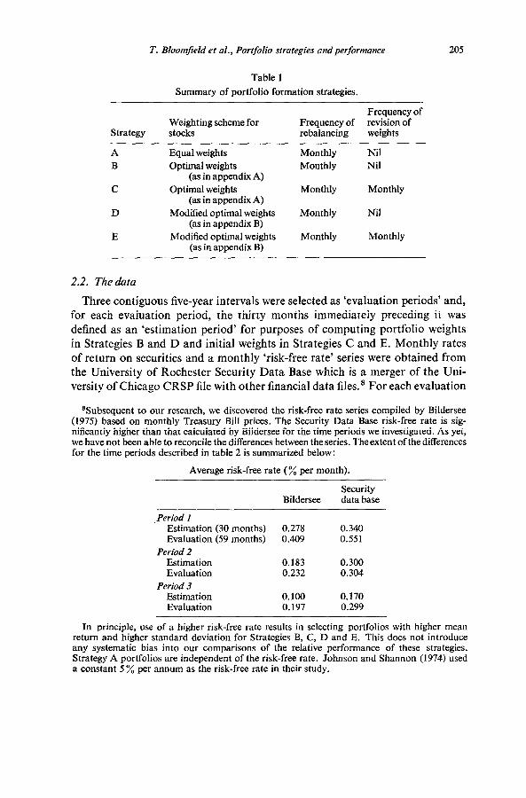
Table 1

Summary of portfolio formation strategies.

Strategy Weighting scheme for stocks

Frequency of Frequency of revision of rebalancing weights

Equal weights Optimal weights

(as in appendix A) Optimal weights

(as in appendix A) Modified optimal weights

(as in appendix B) Modified optimal weights

(as in appendix B)

Monthly Monthly

Monthly

Monthly

Monthly

Nil Nil

Monthly

Nil

Monthly

2.2. The data

Three contiguous five-year intervals were selected as ‘evaluation periods’ and, for each evaluation period, the thirty months immediately preceding it was defined as an ‘estimation period’ for purposes of computing portfolio weights in Strategies B and D and initial weights in Strategies C and E. Monthly rates of return on securities and a monthly ‘risk-free rate’ series were obtained from the University of Rochester Security Data Base which is a merger of the Uni- versity of Chicago CRSP file with other financial data files.8 For each evaluation

“Subsequent to our research, we discovered the risk-free rate series compiled by Bildersee (1975) based on monthly Treasury Bill prices. The Security Data Base risk-free rate is significantly higher than that calculated by Bildersee for the time periods we investigated. As yet, we have not been able to reconcile the differences between the series. Theextent of the differences for the time periods described in table 2 is summarized below:

Average risk-free rate (% per month).

Security Bildersee data base

Period I Estimation (30 months) 0.278 0.340 Evaluation (59 months) 0.409 0.551

Period 2 Estimation 0.183 0.300 Evaluation 0.232 0.304

Period 3 Estimation 0.100 0.170 Evaluation 0.197 0.299

In principle, use of a higher risk-free rate results in selecting portfolios with higher mean return and higher standard deviation for Strategies B, C, D and E. This does not introduce any systematic bias into our comparisons of the relative performance of these strategies. Strategy A portfolios are independent of the risk-free rate. Johnson and Shannon (1974) used a constant 5% per annum as the risk-free rate in their study.


period, all stocks having returns continuously available throughout the period and its associated estimation period were included in the test population.

To assure broad coverage of the test population, a two-stage sampling procedure was used. First, the test population for each evaluation period was

randomly partitioned into non-overlapping subsamples of size 50. Then, when evaluating the strategies for small nominal portfolio sizes (3 5 n I 17), 20 samples of size n were drawn from each of the size-50 subsamples formed in the first stage. Evaluation of the strategies for a nominal portfolio size of 50 was

done by applying the strategies to all of the first-stage size 50 samples. The above characteristics of the test population are summarized in table 2.

Table 2

Data base details.

Period

1 2 3

Stocks Samples of Estimation period Evaluation period available size 50

Feb. 63 -July 65 Aug. 65 -June 70 823 16

March 58 -Aug. 60 Sept. 60 -July 65 877 17

April 53 - Sept. 55 Oct. 55 -Aug. 60 893 17

2.3. Performance measurementfor smallportfolio sizes

The performance of the strategies for small nominal portfolio sizes

(3 < n 5 17) was measured only over evaluation period 1 (Aug. 1965 -June 1970). For that evaluation period the test population was randomly partitioned into 16 non-overlapping samples of 50 stocks each. These samples were indexed

by j = 1, 2, . . . . 16. To evaluate the strategies’ performance for a particular nominal portfolio size n, 20 subsamples (indexed by i = 1, 2, . . . , 20) of size n were drawn in the following way from each of the 16 size-50 samples: From the

jth size-50 sample, a random subsample of size n was drawn without replacement. The identities on the n stocks were noted and they were returned to the 50-stock sample. Repeating this procedure an additional 19 times yielded the 20 subsamples of size n from the jth size-50 sample. When applied to all 16 size-50 samples, 320 size-n subsamples were generated. These subsamples were indexed by(i,j,n),i= 1,2 ,..., 2O;j= 1,2 ,..., 16;n=3,5,7 ,..., 17.

When applied to the stock universe (i, j, n), the rate of return to Strategy X(X = A, B, C, D, E) in month t of the evaluation period was denoted by R, (X, i, j, n). From these rates of return the following summary statistics were

computed :

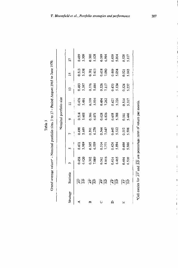
AV(X i,j, n) = f z R,(X, i, j. nh 1-l

Tab

le

3

Gra

nd

aver

age

valu

es”

- N

omin

al

port

folio

si

zes

3 to

17

- Pe

riod

A

ugus

t 19

65 t

o Ju

ne

1970

.

Nom

inal

po

rtfo

lio

size

Stra

tegy

St

atis

tic

3 5

7 9

11

13

15

17

A

AV

0.

458

0.47

1 0.

490

0.51

4 0.

476

0.49

3 0.

513

0.49

9

SD

6.62

0 5.

989

5.68

9 5.

608

5.49

1 5.

397

5.33

8 5.

309

B

AV

0.

392

0.38

5 0.

391

0.38

6 0.

339

0.37

6 0.

381

0.38

0

SD

7.08

9 6.

559

6.27

0 6.

071

5.81

6 5.

684

5.61

3 5.

528

C

AV

0.

541

0.51

4 0.

544

0.62

8 0.

494

0.52

6 0.

618

0.59

9

SD

8.01

6 7.

771

7.64

7 6.

826

7.26

2 7.

117

7.08

0 6.

994

D

AV

0.

414

0.42

4 0.

445

0.45

8 0.

427

0.43

3 0.

449

0.43

9

SD

6.46

5 5.

894

5.51

2 5.

388

5.22

6 5.

124

5.05

4 5.

014

E

Al/

0.49

4 0.

484

0.51

2 0.

541

0.51

4 0.

524

0.52

1 0.

528

SD

6.51

0 5.

886

5.59

8 5.

446

5.31

7 5.

237

5.14

3 5.

117

“Cel

l en

trie

s fo

r A

Tan

d sa

re

perc

enta

ge

rate

s of

ret

urn

per

mon

th.

- -

--.

^_

- ,~

- ,-

. .

.^

- -

. . .

_


.60

2 $ .55 9 s .50 $y

$ .45 s 2 .40 3 2 2 .35 P

.30

0 I j j i 9 11 13 15 17 50

NOMINAL PORTFOLIO SIZE (NO OF ASSETS)

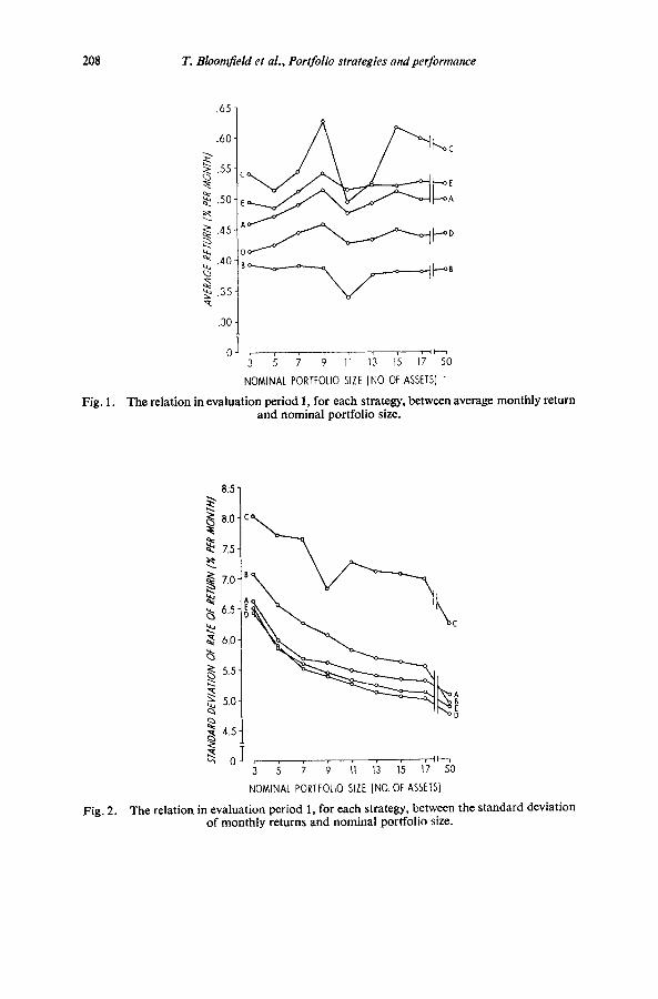
Fig. I. The relation in evaluation period 1, for each strategy, between average monthly return and nominal portfolio size.

, , , , , , , , 3 5 7 9 11 13 15 17 20

NOMINAL PORTFOLIO SIZE (NO. OF ASSETS)

Fig. 2. The relation in evaluation period 1, for each strategy, between the standard deviation of monthly returns and nominal portfolio size.


and

SD(X, i, j, n) = ,zr (R,(X, i,j, n) -AV(X, i,j, n))21+,

forX=A,B,C,D,E;i= 1,2 ,..., 2O;j= 1,2 ,..., 16;andn =3,5,7 ,..., 17. For each strategy and portfolio size, these statistics were then averaged across i andj to yield

Table 4

Average actual portfolio sizes for alternative nominal portfolio sizes and portfolio selection strategies.

Nominal portfolio size

Portfolio selection strategy

A

3 5 I 9

11 13 15 17

3.0 5.0 7.0 9.0

11.0 13.0 15.0 17.0

B C D E

2.0 1.7 2.9 3.0 3.1 2.6 4.9 5.0 4.1 3.2 t’s” 69 4.8 3.9 5.5 4.3 10:8

8’9 10:9

6.2 4.8 12.7 12.9 6.8 5.2 14.7 14.9 7.1 5.6 16.6 16.9

The values of these averages are reported in table 3 and are depicted in figs. 1 and 2. Table 4 gives the average actual portfolio size for each startegy and nominal portfolio size.

2.4. Performance measurement for the large portfolio size

When evaluating the strategies’ performance for the nominal portfolio size of 50, all three of the evaluation periods were used. The symbol R,(X, j, k) denotes the rate of return in month t of evaluation period k for Strategy X when it is applied to the jth 50-stock subsample of period k’s test population. Using this notation, the following statistics were computed:

G


and

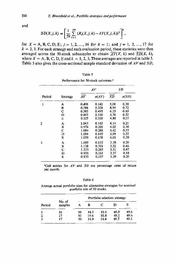
forX=A,B,C,D,E;j=1,2 ,..., 16fork=l;andj=1,2 ,..., 17for k = 2,3. For each strategy and each evaluation period, these statistics were then averaged across the 50-stock subsamples to obtain m(X, k) and %?(X, k),

where X = A, B, C, D, E and k = 1,2, 3, These averages are reported in table 5. Table 5 also gives the cross-sectional sample standard deviation of A V and SD,

Table 5

Performance for 50-stock universes.a

Period

AV SD

Strategy AT u(AV) = o(SD)

I A B C D E

A B C D E

A B C D E

0.498 0.142 5.08 0.30 0.384 0.328 4.94 0.72 0.582 0.495 6.25 0.65 0.443 0.150 4.76 0.32 0.525 0.101 4.88 0.27

1.063 0.142 4.14 0.21 0.974 0.201 4.02 0.30 1.084 0.288 4.42 0.53 1.094 0.145 3.98 0.22 1.059 0.138 4.01 0.20

1.005 0.133 3.38 0.20 1.138 0.311 3.22 0.46 1.233 0.285 3.51 0.47 0.956 0.161 3.37 0.18 0.935 0.157 3.39 0.20

aCell entries for A V and SD are percentage rates of return per month.

Table 6

Average actual portfolio sizes for alternative strategies for nominal portfolio size of 50 stocks.

Portfolio selection strategy No. of

Period samples A B C D E

1 16 50 14.3 10.4 48.9 49.6 2 17 50 19.6 10.8 49.2 49.6 3 17 50 14.9 14.4 49.7 49.3


within each period for each strategy, e.g., a(AV) for Strategy C in period 1 was computed as

Table 6 gives the average actual portfolio sizes for each strategy in each of the evaluation periods.

3. Results

In section 1, three factors affecting estimation and transaction costs were mentioned; (i) portfolio size, (ii) the complexity of the scheme for estimating portfolio weights, and (iii) the frequency of up-dating portfolio weights. The results reported in tables 3 and 5 show variations in average portfolio performance (before estimation and transaction costs) resulting from attempts to reduce costs by restricting portfolio size, using crude estimation techniques, and low frequencies of up-dating portfolio weights. In interpreting these results the following general observations should be kept in mind:

(a) The columns of table 3 are not statistically independent. Both because of overlaps in different size portfolios for a given strategy and because of cross- sectional dependence in the returns of individual securities, it is expected, for instance, that the performance of Strategy B for n = 5 will be positively correlated with B’s performance for n = 13.

(b) In table 3, the performances of different strategies for any given nominal portfolio size are not independent. For some pairs of strategies (e.g., B and C, D and E), the portfolio overlap is such that their returns probably have a very high cross-sectional correlation. The same observation applies, of course, to comparisons of different strategies within a given evaluation period in table 5.

(c) The ‘SD statistics reported in tables 3 and 5 are estimates of the time-series dispersion in monthly strategy returns. The r~(*) statistics reported measures of the cross-sectional (across the 50-stock subsamples) the A Vand SD statistics for each strategy.

in table 5 are dispersion in

3.1. The effects of restrictingportfolio size

With the exception of the somewhat erratic behavior of Strategy C, all strategies exhibited a monotonic decline in the dispersion of their monthly rates of return as nominal portfolio size was increased. In moving from n = 3 to n = 17, there was about a 20% reduction in SD for all strategies (except C). Increasing n from 17 to 50 resulted in a further 5% reduction for all strategies

212 T. Bloomfield et al., Portfolio strategies andperformance

except B and C, for which the reduction was about 10 ‘A. In no case did average monthly return appear to be systematically related to portfolio size.’

Inspection of tables 4 and 6 suggests that the deviant behavior of Strategy C (and, to a lesser extent, Strategy B) can be attributed to its relatively small average actual portfolio size when compared to its nominal portfolio size. This difference between nominal and actual portfolio sizes was emphasized by Johnson and Shannon (1974,1975). When comparing the performance of equally weighted portfolios with the performance of a strategy involving sophisticated estimation of tangency portfolio weights and frequent updating, they found that, with equal nominal portfolio sizes, the two strategies had approximately the same level of dispersion in their monthly rates of return. The average actual portfolio size for the sophisticated strategy, however, was substantially less than its nominal size, i.e., the strategy greatly reduced the number of securities in the portfolio without increasing the variance of portfolio returns. If this empirical result were generally representative, it would indicate a potentially significant benefit of the sophisticated strategy. Johnson and Shannon’s result, however, is not at all confirmed in our study. In tables 3 and 5, Strategies B and C (the two strategies with low actual sizes relative to nominal sizes) have consistently higher dispersion in their monthly returns than do the other strategies. As indicated by the a(*) measures in table 5, Strategies B and C also exhibited much more performance variability across the disjoint 50-stock subsamples than did the other strategies.

3.2. The effects of crude estimation techniques

Among the strategies (B-E) that involve some deliberate attempt to replicate the performance of the tangency portfolio, Strategy D is a crude, low estimation cost analog of Strategy B (B and D both involve a low estimation frequency) and, similarly, Strategy E is the analog of Strategy C (C and E are the high estimation frequency strategies). Except for the comparison of B and D in evaluation period 3 for a nominal portfolio size of 50, the ‘sophisticated’ strategies (B and C) had consistently higher dispersion in their monthly rates of return than did their cruder analogs. Although this was probably due to the smaller actual portfolio sizes of the sophisticated strategies, it was not a result that could have been confidently predicted a priori. Indeed, the latest evidence available prior to our study [see the discussion of Johnson and Shannon (1974, 1975) in section 3.11 indicated the reverse - that in spite of lower actual portfolio sizes, sophisticated estimation techniques do not increase the dispersion of returns.

gAlthough the rank correlation between portfolio size and averale monthly return is significant at the a = 0.20 level (two-tailed test) for Strategies A, B, and E (p = 0.65 for A, p = -0.63 for B, and p = 0.70 for E), the relation is probably spurious. The difference between the maximum and minimum (across portfolio sizes) average monthly returns is less than 0.06% for each of these strategies.

T. Bloomjield et al,, Portfolio strategies andperformance 213

In terms of average monthly returns, there was no statistically significant difference between the performance of the sophisticated strategies and their crude analogs when applied to small security universe (3 I n I 17). The standard deviation of the difference in the monthly returns of Strategies B and D when applied to the same stock universe (similarly for C and E) would be smallest if their returns were perfectly correlated. In that case the standard deviation of the difference in monthly returns would simply be the absolute value of the difference in the strategies’ individual standard deviations. Even under this extreme assumption, however, the results in table 3 indicate no significant difference in average monthly returns. If the same extreme assumption (perfect cross-sectional correlation) is used to estimate the significance of the results for 50-stock universes reported in table 5, the results are ambiguous. Strategy D has a ‘significantly’ higher average return than Strategy B in periods 1 and 2 and vice versa in period 3. There is no significant difference in the average returns on Strategies C and E for periods 1 and 2 and Strategy C does better in period 3.

Strategy A involves no estimation costs at all and, in that sense, is the crudest strategy of all. On an apriori basis, however, Strategy A is not strictly comparable to the other strategies since it does not involve any deliberate attempt to replicate the tangency portfolio. Nevertheless, in our study, Strategy A was not significantly dominated in terms of mean-variance efficiency by any of the other strategies. Indeed, the largest (though probably not significant) difference between A’s performance and that of the other strategies appears in the comparison of A and B for the small portfolio sizes and, in that case, A appears to dominate B.

3.3. The eflects of lowfrequency estimation

One of the techniques for reducing estimation costs is to reduce the frequency of re-estimating portfolio weights on the basis of more recent data. Strategy B is the low estimation frequency analog of Strategy C and, similarly, Strategy D is the low frequency analog of Strategy E.

Judging from the performance statistics in tables 3 and 5, the most consistently observed effect of low estimation frequencies is a reduction in the dispersion of monthly returns. This is most pronounced (as might be expected because of lower actual portfolio sizes) in the comparison of Strategies B and C. Evidently, the month-to-month variability in the portfolio weights for Strategies C and E introduced more variability in monthly strategy returns than it removed by having more ‘up-to-date’ estimates of efficient weights.

The average monthly returns of Strategy B were lower for all portfolio sizes and evaluation periods than the average returns of the high estimation frequency Strategy C. Even under the extreme assumption of perfect cross-sectional correlation (explained above in section 3.2), however, the difference in B and C’s returns is ‘significant’ only for size-50 portfolios in periods 2 and 3. Because of


the relatively small difference in the dispersion of Strategies D and E’s monthly returns, the extreme assumption of perfect cross-sectional correlation implies that the average returns of Strategy E (a high frequency strategy) are ‘significantly’ greater then the average returns of Strategy D for small portfolio sizes. This pattern is reversed, however, for size-50 portfolios in two out of the three evaluation periods.

4. Interpretation and conclusion

On the basis of our empirical measurements of the performance of alternative portfolio strategies we conclude that:

(a) The choice of the size of the security universe to which any given strategy is applied is a non-trivial matter. Increasing the size of the security universe clearly reduces the dispersion of monthly rates of return to the portfolio strategy. Just as clearly, however, the transaction and estimation costs of implementing the strategy will, for most investors, be an increasing function of the security universe size.

(b) To the extent that they are significantly more expensive to implement than relatively naive strategies, strategies that involve complex (and purportedly more accurate) calculations of ‘optimal’ portfolio weights are not worth employing. The complex strategies we evaluated exhibited consistently greater dispersion in their monthly returns than did their more naive analogs applied to the same stock universes. At the same time, the average monthly returns (before implementation costs) of the complex strategies were not significantly greater than those of the cruder strategies. Ironically, this failure of the complex strategies probably is due to their complexity. Given the ‘true’ values of the security return distribution parameters (means, variances, and covariances) the complex strategies would, by construction, yield more accurate estimates of tangency portfolio weights than the more naive strategies. Because they are much more complicated functions of the distribution parameters, however, the weight esti- mators in the complex strategies are more sensitive to measurement errors in those parameters. Thus, in the process of arriving at portfolio weights, ‘noise’ in estimates of the distribution parameters is magnified more in the complex strategies than in the naive strategies and, at least in our simulations, this noise was more than enough to offset the potential superiority of the complex strategies.

(c) Frequent up-dating of ‘optimal’ portfolio weights increases the dispersion of returns without significantly or unambiguously increasing the average level of returns (before transaction and estimation costs). This is to be expected if the joint distribution of monthly security returns is relatively stationary and does not exhibit significant serial dependence. To the extent that frequent up-dating of calculated portfolio weights is costly, our results indicate at least that the optimal up-dating interval is longer than one month.


Appendix A”

From time series regressions of monthly stock returns on monthly returns to an ‘index portfolio’, estimates of the following parameters are obtained:

(i) pi = the ‘beta’ of stockj, (ii) vj = the residual variance from the regression for stockj,

(iii) pj = the expected excess of stock j’s return above the risk-free rate of return,

(iv) 0; = the variance of the rate of return on the index portfolio.

It is assumed in the algorithm below that the covariance structure of stock returns is given by

bij = PTal2 +Ui, i = j,

= BiPjgI” 3 i#j,

where ~ii is the variance of stock i’s return and cij is the covariance between the returns of stocks i and j. It is also assumed that pj > 0 for at least one stock.

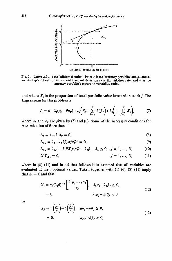
In fig. 3, the ‘tangency’ portfolio is represented by T, the point where a straight line from the risk-free asset (0, rp) is tangent to the ‘efficient frontier’, BC, of the set of feasible stock portfolios.

The problem of determining the composition of the tangency portfolio is then equivalent to the problem of finding the portfolio P that maximizes the angle 8 subject to the constraints

Pp = fJOP, (1)

(2)

(3)

Xj 2 0, j = 1, . . . . N, (4)

where pp and a, are given by

(5)

(6)

“‘Although developed independently, the algorithm described in appendix A is equivalent to an algorithm proposed by Elton, Gruber, and Padberg (1976).


STANDARD DEVIATION OF RETURN

Fig. 3. Curve ABC is the ‘efficient frontier’. Point Tis the ‘tangency portfolio’ and ps and uT are its expected rate of return and standard deviation r, is the risk-free rate, and 0 is the

taugency portfolio’s reward-to-variability ratio.

and where Xj is the proportion of total portfolio value invested in stockj. The Lagrangean for this problem is

where pP and o, are given by (5) and (6). Some of the necessary conditions for maximization of 8 are then

L, = 1 -L,t+ = 0, (8)

Lb&. = &-1,e&J,Zo;’ = 0, (9)

LX, = ~~~j-~,~xjVj~~‘-~,~j-~, 5 0, j = 1, . . . . N, (10)

XjLX, = 0, j= l,...,N, (11)

where in (Q-(11) and in all that follows it is assumed that all variables are evaluated at their optimal values. Taken together with (l)-(6), (Q-o-(l) imply that A3 = 0 and that

or

Xi = o(~)-b(~), a/t,-bPj 2 0,

(13)


where

a z 8-‘ap and b G A,t~~,/~,8. (14)

Let J be the index set such that Xj > 0 if j E J and Xj = 0 if j $ J. Then, since

E JEJ Xj = 1 and C ,e~ Xjfij = pp = (&~,/n,@(ai)-’ [from (9)] = b(c$-’ [from (14)], the ratio y z b/a can be solved for, and

xj = (a/oj> Olj-YPj), _icJ, (1%

where

(16)

All that now remains is to find the optimal index set J. This can be accomplished by the following algorithm:

(i) Index the stocks such that

P1/1PII 2 PZllPZl 2 **a 2 /+dIBNI. (ii) Let Yj be defined as y computed from (16) for the index set J = { 1,2, . . . , j}.

(iii) The optimal index set is J = {1,2, . . . , k} where k is the smallest index for which ,uk+ i --Y&+~ 5 0 unless pN - y& > 0 in which case J= {1,2 ,..., N}.

Given J, the optimal portfolio weights are then computed from (15) with a chosen SO that Cj EJ Xi = 1.

In actual application of the algorithm to small security universes (e.g., N = 3), it may be the case that all estimated mean excess returns are negative, i.e., ~j < 0, j = 1, . . . . N. In these cases, we used the rule of placing all funds in the risk-free asset. In our study, this situation occurred only in period 1 for Strategies B and C. In the case of Strategy B it occurred only for N = 3 and then only for 5 out of the 320 size-3 universe sampled. For Strategy C, which involved monthly reestimation of portfolio weights and hence 18,880 applications of the algorithm for each value of N, the situation arose in 6.5% of the applications for N = 3; 2%forN= 5;0.7%forN= 7;0.4%forN=9;0.2%forN= ll;O.O4%for N = 13;0.04%forN = 15;andO.O3%forN = 17.

Appendix B

If it is assumed that all stocks plot on the ‘security market line’, i.e., that

2 = 2 = . . . = 2, (17)


then from (15) and (16) in appendix A

where Kis chosen so that

~ Xj= 1. I=2

In all applications of this simplified algorithm, there was never a case in which bj < 0, j = 1, . . . . N. Had there been such a case, however, the implied investment rule would be to put all funds in the risk-free asset.

References

Bildersee, J.S., 1975, Some new bond indexes, Journal of Business 48, 506-525. Blume, M.E., 1970, Portfolio theory: A steu towards its practical an&cation. Journal of

Business 43, 1521173. __

Cohen, K.J. and J.A. Pogue, 1967, An empirical evaluation of alternative portfolio.seIection models. Journal of Business 40. 166193.

Elton, E.J;, M.G. Gruber and M.W. Padberg, 1976, Simple criteria for optimal portfolio selection, Journal of Finance 31, 1341-1357.

Evans, J.L., 1970, An analysis of portfolio maintenance strategies, Journal of Finance 25, 561-571.

Evans, J.L. and S.H. Archer, 1968, Diversification and the reduction of dispersion: An empirical analysis, Journal of Finance 23, 761-767.

Fama, E.F., 1976, Foundations of finance (Basic Books, New York). Johnson, K.H. and D.S. Shannon, 1974, A note on diversification and reduction of dispersion,

Journal of Financial Economics 1, 365-372. Johnson, K.H. and D.S. Shannon, 1975, Portfolio maintenance strategies revisited, Atlantic

Economic Journal 3,25-35. Markowitz, H., 1952, Portfolio selection, Journal of Finance 7,77-91. Markowitz, H., 1956, The optimization of a quadratic function subject to linear constraints,

Naval Research Logistics Quarterly 3, 111-133. Markowitz, H., 1959, Portfolio selection: Efficient diversification of investments (Wiley,

New York). Sharpe, W.F., 1963, A simplified model for portfolio analysis, Management Science 9,277-293. Sharpe, W.F., 1967, Portfolio analysis, Journal of Financial and Quantitative Analysis 2,

7684. Tobin, J., 1958, Liquidity preference as behavior towards risk, Review of Economic Studies 25,

65-86.

Portfolio strategies and performance

Documents