PORTFOLIO OPTIMIZATION WITH HEDGE FUNDS: Conditional …

ETH Library

Portfolio optimization with hedgefundsConditional value at risk and conditional draw-downat risk for portfolio optimization with alternativeinvestments

Master Thesis

Author(s):Jöhri, Stephan

Publication date:2004

Permanent link:https://doi.org/10.3929/ethz-a-004696440

Rights / license:In Copyright - Non-Commercial Use Permitted

This page was generated automatically upon download from the ETH Zurich Research Collection.For more information, please consult the Terms of use.

https://doi.org/10.3929/ethz-a-004696440

http://rightsstatements.org/page/InC-NC/1.0/

https://www.research-collection.ethz.ch

https://www.research-collection.ethz.ch/terms-of-use

PORTFOLIO OPTIMIZATION WITH HEDGE FUNDS:

Conditional Value At Risk And Conditional Draw-Down At Risk

For Portfolio Optimization With Alternative Investments

Stephan Johri ∗

Supervisor: PD Dr. Diethelm WurtzProfessor: Dr. Kai Nagel

March 16, 2004

∗Master’s Thesis of Stephan Johri written at the department of Computer Science of Swiss Federal Instituteof Technology (ETH) Zurich.

1

Abstract

The aim of this Master’s Thesis is to describe and assess different ways to optimize a portfolio.Special attention is paid to the influence of hedge funds since their returns exhibit special sta-tistical properties.

In the first part of this thesis modern portfolio theory is considered. The Markowitz ap-proach is described and analyzed. It assumes that the assets are identically independentlydistributed according to the Normal law. CAPM and APT are briefly reviewed.

In the second part we go beyond Markowitz and show that asset returns are in reality notnormally distributed, but have fat tails and asymmetries. This is especially true for the returnsof hedge funds. These facts justify further investigations for alternative portfolio optimizationtechniques. We describe and discuss therefore alternative methods that can be found in lit-erature. They use risk measures different than the standard deviation like Value at Risk orDraw-Down and their derivations Conditional Value at Risk and Conditional Draw-Down atRisk. Based on these methods, the respective optimization problems are formulated and im-plemented.

In the third part we describe the numerical implementation and the used data. Finally theweight allocations and efficient frontiers that summarize the results of these optimization prob-lems are calculated, analyzed and compared. We focus on the question how optimal portfolioswith and without hedge funds are constructed according to the different optimization methods,how useful these methods are in practice and how the results differ. The results are derived byanalytical work and simulations on historical and artificial data.

2

Acknowledgment

I would like to thank my supervisor PD Dr. Diethelm Wurtz for directing this thesis andguiding me with a lot of useful impulses. I am also thankful to Prof. Kai Nagel who gave mythe opportunity to work on this topic.My gratefulness belongs also to the people at UBS Investment Research Dr. Marcos Lopez dePrado, Dr. Achim Peijan, Laurent Favre and Dr. Klaus Kranzlein who gave me a lot of inputsduring our discussions.

3

4

Contents

I Modern Portfolio Theory 7

1 Markowitz Model 71.1 Risk Return Framework And Utility Function . . . . . . . . . . . . . . . . . . . . 71.2 Selecting Optimal Portfolios: The Efficient Frontier . . . . . . . . . . . . . . . . . 14

2 Capital Asset Pricing Model (CAPM) 272.1 Standard Capital Asset Pricing Model . . . . . . . . . . . . . . . . . . . . . . . . 272.2 Arbitrage Pricing Theory (APT) . . . . . . . . . . . . . . . . . . . . . . . . . . . 30

II Beyond Markowitz 34

3 Stylized Facts Of Asset Returns 343.1 Distribution Form Tests . . . . . . . . . . . . . . . . . . . . . . . . . . . . . . . . 353.2 Dependencies Tests . . . . . . . . . . . . . . . . . . . . . . . . . . . . . . . . . . . 383.3 Results Of Statistical Tests Applied To Market Data . . . . . . . . . . . . . . . . 42

4 Portfolio Construction With Non Normal Asset Returns 484.1 Introduction To Risk In General . . . . . . . . . . . . . . . . . . . . . . . . . . . 484.2 Variance As Risk Measure . . . . . . . . . . . . . . . . . . . . . . . . . . . . . . . 50

5 Value At Risk Measures 525.1 Value At Risk . . . . . . . . . . . . . . . . . . . . . . . . . . . . . . . . . . . . . . 525.2 Conditional Value At Risk, Expected Shortfall And Tail Conditional Expectation 545.3 Mean-Conditional Value At Risk Efficient Portfolios . . . . . . . . . . . . . . . . 58

6 Draw-Down Measures 606.1 Draw-Down And Time Under-The-Water . . . . . . . . . . . . . . . . . . . . . . 606.2 Conditional Draw-Down At Risk And Conditional Time Under-The-Water At Risk 616.3 Mean-Conditional Draw-Down At Risk Efficient Portfolios . . . . . . . . . . . . . 65

7 Comparison Of The Risk Measures 67

III Optimization With Alternative Investments 68

8 Numerical Implementation 68

9 Used Data 699.1 Normal Vs. Logarithmic Data . . . . . . . . . . . . . . . . . . . . . . . . . . . . . 699.2 Empirical Vs. Simulated Data . . . . . . . . . . . . . . . . . . . . . . . . . . . . . 70

10 Evaluation Of The Portfolios 7210.1 Evaluation With Historical Data . . . . . . . . . . . . . . . . . . . . . . . . . . . 7210.2 Evaluation With Simulated Data . . . . . . . . . . . . . . . . . . . . . . . . . . . 76

Summary and Outlook 82

5

Appendix 84

A Quadratic Utility Function Implies That Mean Variance Analysis Is Optimal 84

B Equivalence Of Different VaR Definitions And Notations 85

C Used R Functions 86

D Description Of The Portfolio Optimization System 87

E Description Of The Excel Optimizer 89

F Description Of Various Hedge Fund Styles 90

G References 92

6

Part I

Modern Portfolio Theory

1 Markowitz Model

In this first chapter the fundamentals of portfolio theory are introduced. This is done by showingsome statistical properties, deriving a utility function and presenting the model that combinesboth for portfolio optimization. This model was developed in 1952/59 by Harry Markowitz andis still considered as the standard approach for this task.

1.1 Risk Return Framework And Utility Function

Risk Return Framework

Assuming we are given N assets with their returns R1, ..., RN respectively. Our portfolio consistsof these assets with a fraction of w1, ..., wN invested in each asset. Then the expected returnsof the individual assets would be E[Ri] = µi (where E[] indicates the expected value) and thetotal return µP of the portfolio

µP =N∑

i=1

wiµRi (1)

Two properties of the mean value that will become useful later:

µRi+Rj = µRi + µRj

µcRi = cµRi

The first property means that the mean of the sum of two return series i and j are the same asthe mean of return series i plus the mean of return series j. The second property states thatthe mean of a constant c multiplied with a return series is equal to c times the mean of thereturn series i.The variance of the portfolio will be

σ2P = E[(RP − µP )2] =

N∑i=1

wi(Ri − µP )2 =N∑

i=1

(wiσi)2 + 2N−1∑i=1

N∑j=i+1

wiwjσij (2)

So in the case of three assets we get the following pattern:

σ2P = (w1σ1)2 + (w2σ2)2 + (w3σ3)2 + 2w1w2σ12 + 2w1w3σ13 + 2w2w3σ23

7

These variances σ2i = E[(RP − µP )2] and covariances σij = E[(Ri − µi)(Rj − µj)] = σji are

collected in symmetric matrix called covariance matrix:

C =

σ2

1 σ12 · · · σ1N

σ12 σ22 σ2N

.... . .

...σ1N σ2N · · · σ2

N

(3)

The correlation is defined as the standardized covariance:

ρij =σij

σiσj(4)

Comparing (1) and (2) we can see the effect of diversification: The return of a portfolio cannever be smaller than the smallest return of its constituents, since it is the weighted averagereturn of all constituents. In contrast, the variance of a portfolio can be smaller than the smallestvariance of its individual assets because of the second term of (2) which can be negative in caseof a negative covariance between the asset returns. So the aim of diversification is to chose theassets in a way to keep the mean return high and lower the variance by an appropriate selectionand weighting of the assets.

Taking (2) with equal amount of investments in each of the N assets we get

σ2P =

1N

σi2 +

N − 1N

σij (5)

whereby the first term is called diversifiable or non market risk and the second termsystematic or market risk. If we take a large amount of different assets (N approachinginfinity), the portfolio risk gets reduced to the average covariance of the assets in the portfolioand all the variances of the assets disappear.

σ2P −−−−→

N→∞σij

This effect shows us that the first term in (5) is called diversifiable risk because it can bereduced to zero by a good diversification of the assets. The risk represented in the first termof (5) has its origin in the risk of the single assets the portfolio contains, whereas the riskexpressed in the second term is coming from the market itself (which can be influenced byeconomic changes or events with a large impact) and can not be reduced.This also means that the risk of a portfolio of assets with a low correlation can be more re-duced than the risk of a portfolio existing of highly correlated assets. In practice this resultsin the recommendation to choose the constituents of a portfolio from different geographic orindustrial sectors, because assets of companies from the same country or business areas tend tomove together and have hence a higher correlation. Figure 1 shows an example exhibiting thiseffect for the case of securities from the UK and the US.

In a risk return framework a high risk gets usually compensated by a high expected return.This is called risk premium: The extra return a particular asset has to provide over the rate ofthe market to compensate for market risk. The drawback of diversification is that the investorlooses the risk premium that a certain asset might provide since its contribution on the finalportfolio return is very small. The advantage of a well diversified portfolio however, is that onecan expect a more moderate but constant return on the long run.

8

0 5 10 15 20 25 30

0.0

0.2

0.4

0.6

0.8

1.0

Number of assets

Ris

k

Figure 1: This chart shows the risk of a portfolio versus the number of assets the portfolio contains.We can see that a portfolio with few assets has a higher risk than a portfolio with lots of assets (effect ofdiversification). The doted line represents a portfolio consisting of stocks from the UK whereas the solidline depicts a portfolio with US stocks. Since the line for the UK portfolio is higher, we can concludethat the stocks in UK have a higher average covariance and their risk can therefore less reduced in aportfolio as the risk of a portfolio consisting of US stocks.

Utility Function Of An Investor

Bernoulli proposed in [9] that the value of an item should not be determined by the pricesomebody has to pay for it but by the utility that this item has for the owner. A classicalexample would be that a glass of water has a much higher utility for somebody who is lost inthe dessert than for somebody in the civilization. Although the glass of water might be exactlythe same and therefore its price, two persons in the mentioned situations will perceive its valuedifferently.

We will now discuss the properties that such an utility function should have and look atsome typical economic utility functions. The structure of this section will partially follow theone in Elton&Gruber [18].

The first property we want to have fulfilled is that an investor prefers more to less. Economistscall this the non-satiation attribute. It expresses the fact that an option with a higher re-turn has always a higher utility than an option with a lower return assuming that both optionsare equally likely. Or as a shorter expression, everybody prefers more wealth than less wealth.From this we can conclude that the first derivative of the utility function always has to bepositive. Our first requirement for a utility function U() for a wealth parameter W is therefore

U ′(W ) > 0

As a second attribute we want to include the investors risk profile. Bernoulli uses a fairgamble to introduce this concept. A fair gamble is a game where the expected gain is equalto zero. This means that the probability of a gain times the value of the gain is equal to theprobability of a loss times the loss in absolute terms. To toss a coin would be a fair gamble if oneplayer wins both investments when one side is up and the other payer wins both investmentswhen the other side is up. We will examine three types of risk profiles.

9

Wealth

Util

ity

Figure 2: A logarithmic utility function seems to be appropriate in the context of a risk averse investor.The increase of the utility function for a certain increase in the wealth is smaller if the investor is alreadyon a high level of wealth

Risk aversion is defined as rejecting a fair gamble. A risk averse investor would not playa game where he or she has an expected return of zero in the long run. Let’s find out whatthe implications for a risk averse investor are: Since he or she does not invest, we can concludethat the utility for keeping the current wealth is higher than the probability weighted utilityfor a gain and loss. We can describe this risk profile for the case of a fair gamble as

U(W ) >12U(W + G) +

12U(W −G)

where W is the current wealth and G the symmetric gain/loss of the game.Multiplying by 2 and rearranging yields to

U(W )− U(W −G) > U(W + G)− U(W )

and we can see that such an investor prefers the change from the current wealth minus thegain/loss to the current wealth than the change from the current wealth to the current wealthplus the gain/loss. Note that the absolute change in wealth is in both cases the same (G). Fromthis we see that a risk averse investor prefers to keep all of his/her fortune rather than to investa part of it and loss or gain with a 50% probability an equal part. Functions that satisfy thisrequirement have the second derivative smaller than zero.

U ′′(W ) < 0

Figure 2 shows a logarithmic utility function that fulfills this property. We can see that for thedouble amount of wealth, the additional amount of utility is less then the double. Formulatedaccording to the example with the fair gamble the figure expresses that for the same amount ofincrease in the utility the investor asks for a higher increase in the wealth the higher the wealthalready is.

As second risk profile we have a look at the risk neutral investor. This is defined as aninvestor which is indifferent to a fair gamble. He or she will sometimes play and sometimes not.

10

Wealth

Util

ity

Figure 3: Utility functions for a risk averse investor (solid), risk neutral investor (doted) and a riskseeking investor (dashed) in a wealth/utility framework

For such a person the utility equation looks like

U(W ) =12U(W + G) +

12U(W −G)

We can rearrange this again and get

U(W )− U(W −G) = U(W + G)− U(W )

this means that such a person is indifferent about the preference of the change from the currentwealth minus the gain/loss to the current wealth than the change from the current wealth tothe current wealth plus the gain/loss. Hence risk neutrality causes the second derivative of theutility function to be zero.

U ′′(W ) = 0

Risk seeking is called the third risk profile and it is defined as accepting a fair gamble.These kind of investors agree to the following formulations

U(W ) <12U(W + G) +

12U(W −G)

U(W )− U(W −G) < U(W + G)− U(W )

we can assign them a utility function with a positive second derivative since the wealthier theyare the more they will appreciate an additional increment in their wealth.

U ′′(W ) > 0

To conclude, in figure 3 the utility functions are drawn in a wealth/utility framework forthe three risk types.

11

We can also transform the utility function to the Mean-Variance framework. In [27] thefollowing utility function is proposed for this purpose

µU = µR − λσ2

where µU is the expected utility, µR the expected return, σ the standard deviation of returnsand λ the risk-aversion coefficient.With λ the function can get adapted to the investors aversion to risk. A positive coefficientindicates risk aversion, λ = 0 means risk neutrality and a negative coefficient defines a riskseeking investor. A typical level of risk aversion would be around 0.0075, as stated in [24].

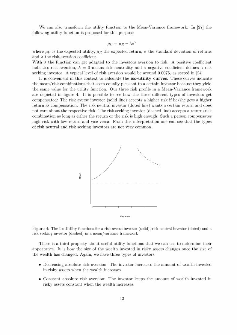
It is convenient in this context to calculate the iso-utility curves. These curves indicatethe mean/risk combinations that seem equally pleasant to a certain investor because they yieldthe same value for the utility function. Our three risk profile in a Mean-Variance frameworkare depicted in figure 4. It is possible to see how the three different types of investors getcompensated: The risk averse investor (solid line) accepts a higher risk if he/she gets a higherreturn as compensation. The risk neutral investor (doted line) wants a certain return and doesnot care about the respective risk. The risk seeking investor (dashed line) accepts a return/riskcombination as long as either the return or the risk is high enough. Such a person compensateshigh risk with low return and vise versa. From this interpretation one can see that the typesof risk neutral and risk seeking investors are not very common.

Variance

Mea

n

Figure 4: The Iso-Utility functions for a risk averse investor (solid), risk neutral investor (doted) and arisk seeking investor (dashed) in a mean/variance framework

There is a third property about useful utility functions that we can use to determine theirappearance. It is how the size of the wealth invested in risky assets changes once the size ofthe wealth has changed. Again, we have three types of investors:

• Decreasing absolute risk aversion: The investor increases the amount of wealth investedin risky assets when the wealth increases.

• Constant absolute risk aversion: The investor keeps the amount of wealth invested inrisky assets constant when the wealth increases.

12

• Increasing absolute risk aversion: The investor decreases the amount of wealth investedin risky assets when the wealth increases.

It can be shown that

A(W ) =−U ′′(W )U ′(W )

measures the absolute risk aversion of an investor. As a consequence, we can define the investortypes according to A′(W ) and assign it as follows:A′(W ) > 0: Increasing absolute risk aversionA′(W ) = 0: Constant absolute risk aversionA′(W ) < 0: Decreasing absolute risk aversionIt is also possible to use the change in the relative investment as property. This is expressed by

R(W ) =−WU ′′(W )

U ′(W )= WA(W )

and interpreted as follows:R′(W ) > 0: Increasing relative risk aversionR′(W ) = 0: Constant relative risk aversionR′(W ) < 0: Decreasing relative risk aversion

It is commonly accepted that most investors exhibit decreasing absolute risk aversion, butthere is no agreement concerning the relative risk aversion.

In [18] two common utility functions are presented: The most frequently used utility functionin economics is the quadratic one. It is preferred because the assumption of a quadratic utilityfunction implies that the mean variance analysis is optimal (see Appendix A for a prove).

U(W ) = aW − bW 2 (6)

This utility function has the following first and second derivatives

U ′(W ) = a− 2bW

U ′′(W ) = −2b

To make this utility function compliant to the requirements of a risk averse investor, we have toset the second derivative to be smaller than zero or b positive. We have shown that an investorusually prefers more to less and asks therefore the first derivative to be positive or W < 1

2b .An analysis of the absolute and relative risk-aversion measures show that the quadratic utilityfunction has an increasing absolute and relative risk aversion.

Since the quadratic utility function has some undesired properties, there are other utilityfunctions in use that also satisfy mean variance analysis like

U(W ) = lnW

with its first and second derivativesU ′(W ) =

1W

U ′′(W ) = − 1W 2

It gets clear that the first derivative is positive for all values of W and the second derivativeis negative for all values of W . So the logarithmic utility function also meets the requirementsof a risk averse investor who prefers more to less. Further this function exhibits decreasingabsolute risk aversion and constant relative risk aversion.

13

1.2 Selecting Optimal Portfolios: The Efficient Frontier

The basic set-up of the Markowitz [30] model is as follows:

wT Cw → Min (7)

s.t.

wT µ = µP > 0 (8)

wT e = 1

where e = (1, 1, ..., 1)T , C is the Covariance Matrix as defined in (3), µ is the expected returnvector of the assets and µP is the desired expected return of the portfolio. The first line ofthe set-up defines that we want to minimize the variance and therefore the risk of the finalportfolio. In the second expression we fix the expected return of the portfolio to a chosen value.It is evident that we are only interested in a return larger than zero. The last constraint setsthe sum of the weights to one since we want to be fully invested.

In a short sale a trader sells an asset that is not in its possession to buy it later back andequalize its balance sheet. This practice makes sense in expectation of a decreasing price. Shortsales are indicated by negative asset weights in a portfolio, since the owner of the portfolio hassold something that does not belong to him/her. If no short sales are allowed, which is usuallythe case, there will be an additional constraint:

wi ≥ 0

We will formulate the solution of the system according to de Giorgi [15]. Equations (7) and(8) describe a quadratic objective function with linear constraints. If the covariance matrix Cis strictly positive finite, a portfolio will solve the optimization problem iff

w(µP ) = µP w0 − w1 (9)

where

w0 =1S

(QC−1µ−RC−1e)

w1 =1S

(RC−1µ− PC−1e)

with

P = µT C−1µ

Q = eT C−1e

R = eT C−1µ

S = PQ−R2

With (9) we can determine the optimal portfolio for a given expected portfolio return. Thisformula also sets the expected portfolio return µP into a relation to the portfolio variance σP

which is

σ2P1Q

−(µP − R

Q)2

SQ2

= 1 (10)

14

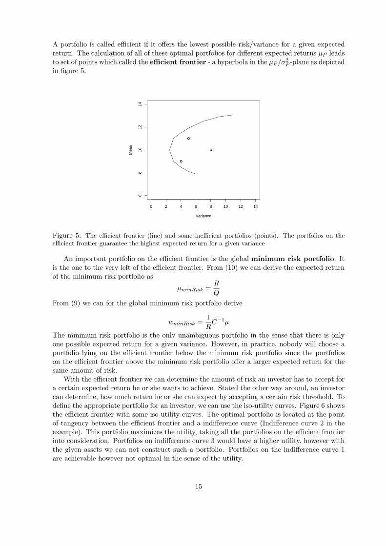
A portfolio is called efficient if it offers the lowest possible risk/variance for a given expectedreturn. The calculation of all of these optimal portfolios for different expected returns µP leadsto set of points which called the efficient frontier - a hyperbola in the µP /σ2

P -plane as depictedin figure 5.

0 2 4 6 8 10 12 14

68

1012

14

Variance

Mea

n

●

●

●

Figure 5: The efficient frontier (line) and some inefficient portfolios (points). The portfolios on theefficient frontier guarantee the highest expected return for a given variance

An important portfolio on the efficient frontier is the global minimum risk portfolio. Itis the one to the very left of the efficient frontier. From (10) we can derive the expected returnof the minimum risk portfolio as

µminRisk =R

Q

From (9) we can for the global minimum risk portfolio derive

wminRisk =1R

C−1µ

The minimum risk portfolio is the only unambiguous portfolio in the sense that there is onlyone possible expected return for a given variance. However, in practice, nobody will choose aportfolio lying on the efficient frontier below the minimum risk portfolio since the portfolioson the efficient frontier above the minimum risk portfolio offer a larger expected return for thesame amount of risk.

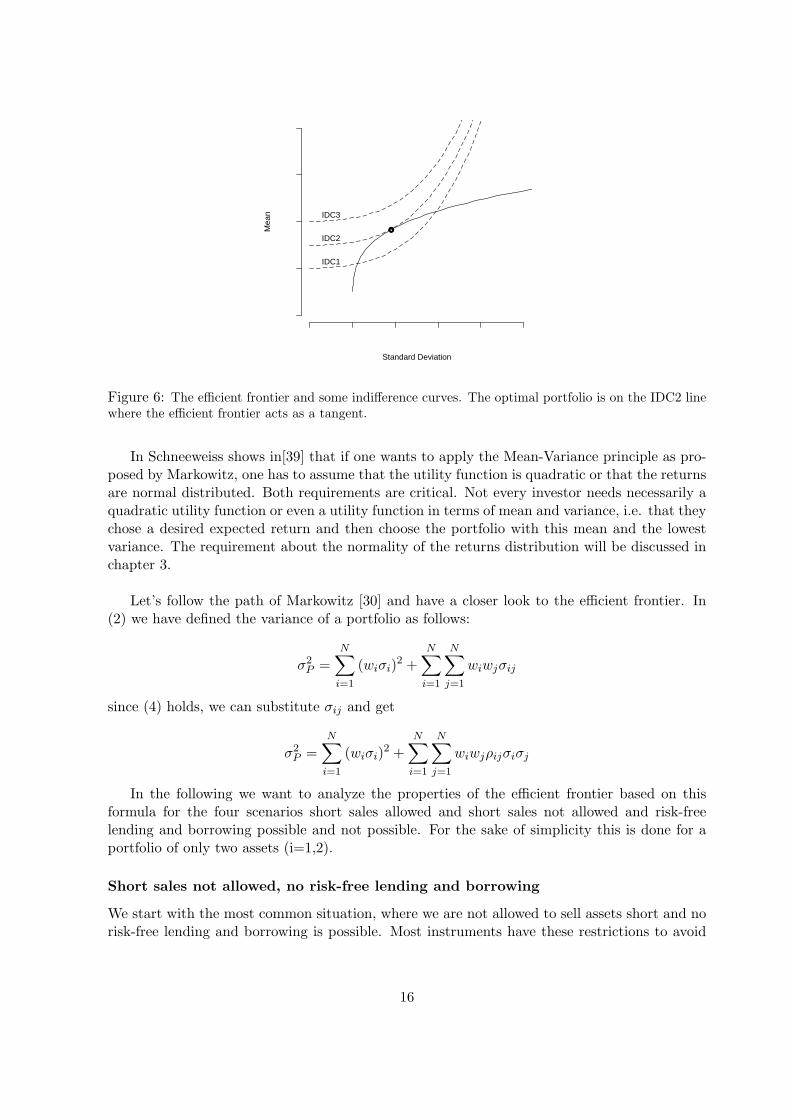
With the efficient frontier we can determine the amount of risk an investor has to accept fora certain expected return he or she wants to achieve. Stated the other way around, an investorcan determine, how much return he or she can expect by accepting a certain risk threshold. Todefine the appropriate portfolio for an investor, we can use the iso-utility curves. Figure 6 showsthe efficient frontier with some iso-utility curves. The optimal portfolio is located at the pointof tangency between the efficient frontier and a indifference curve (Indifference curve 2 in theexample). This portfolio maximizes the utility, taking all the portfolios on the efficient frontierinto consideration. Portfolios on indifference curve 3 would have a higher utility, however withthe given assets we can not construct such a portfolio. Portfolios on the indifference curve 1are achievable however not optimal in the sense of the utility.

15

Standard Deviation

Mea

nIDC1

IDC2

IDC3

●●●●●

Figure 6: The efficient frontier and some indifference curves. The optimal portfolio is on the IDC2 linewhere the efficient frontier acts as a tangent.

In Schneeweiss shows in[39] that if one wants to apply the Mean-Variance principle as pro-posed by Markowitz, one has to assume that the utility function is quadratic or that the returnsare normal distributed. Both requirements are critical. Not every investor needs necessarily aquadratic utility function or even a utility function in terms of mean and variance, i.e. that theychose a desired expected return and then choose the portfolio with this mean and the lowestvariance. The requirement about the normality of the returns distribution will be discussed inchapter 3.

Let’s follow the path of Markowitz [30] and have a closer look to the efficient frontier. In(2) we have defined the variance of a portfolio as follows:

σ2P =

N∑i=1

(wiσi)2 +N∑

i=1

N∑j=1

wiwjσij

since (4) holds, we can substitute σij and get

σ2P =

N∑i=1

(wiσi)2 +N∑

i=1

N∑j=1

wiwjρijσiσj

In the following we want to analyze the properties of the efficient frontier based on thisformula for the four scenarios short sales allowed and short sales not allowed and risk-freelending and borrowing possible and not possible. For the sake of simplicity this is done for aportfolio of only two assets (i=1,2).

Short sales not allowed, no risk-free lending and borrowing

We start with the most common situation, where we are not allowed to sell assets short and norisk-free lending and borrowing is possible. Most instruments have these restrictions to avoid

16

speculations and high risks. Three sub cases are investigated, dependent on the value of thecorrelation ρ between the asset returns.

Perfect positive correlation (ρ = 1) with w2 = 1−w1, mean and variance of the portfoliobecome

µP = w1µ1 + (1− w1)µ2 (11)

σ2P = (w1σ1 + (1− w1)σ2)2 (12)

It shows that with totally correlated assets, return and risk of a portfolio is just the weightedaverage of return and risk of its components. By solving (11) for w1 and substituting w1 into(12), one gets

µP = (µ2 −µ1 − µ2

σ1 − σ2σ2) + (

µ1 − µ2

σ1 − σ2)σP

which is the equation of a straight line. So the efficient frontier for positive correlated assets isa linear combination of the given assets as shown in figure 7.

0 2 4 6 8 10 12 14

68

1012

14

Variance

Mea

n

●

●

Asset 1

Asset 2

Figure 7: The efficient frontier of two assets with perfect correlation is a straight line.

Perfect negative correlation (ρ = −1) In the case of a perfect negative correlation, meanand variance of the portfolio become

µP = w1µ1 − (1− w1)µ2

σ2P = (w1σ1 − (1− wi)σ2)2 = (−w1σ1 + (1− wi)σ2)2 (13)

In the same way as in the case of positive correlation, we can find, that the efficient frontierconsists of two straight lines (one for each result of the square root of (13)) drawn in figure 8. If

17

we have perfectly anti-correlated assets, it is always possible to find combination of them whichhas zero risk. The appropriate weight and return can be found by setting (13) equal to zero.

w1 =σ2

σ1 + σ2

µP ∗ =µ1σ2 − µ2σ1

σ1 + σ2

0 2 4 6 8 10 12 14

68

1012

14

Variance

Mea

n

●

●

●

Asset 1

Asset 2

Figure 8: The efficient frontier of two assets with perfect negative correlation. It shows that the upperline has the equation µP ∗ = aσP + µP ∗ whereby the lower line is µP ∗ = −aσP + µP ∗ with a as aconstant. The two lines intersect the y-axis at µP ∗

No relationship between returns of the assets (ρ = 0) For this scenario the variance ofthe portfolio gets simplified to

σ2P = (w1σ1)2 + ((1− w1)σ2)2

To find the minimum risk portfolio, one sets ∂σP∂wi

= 0 and receives for the case of two assets

w1 =σ2

2

σ21 + σ2

2

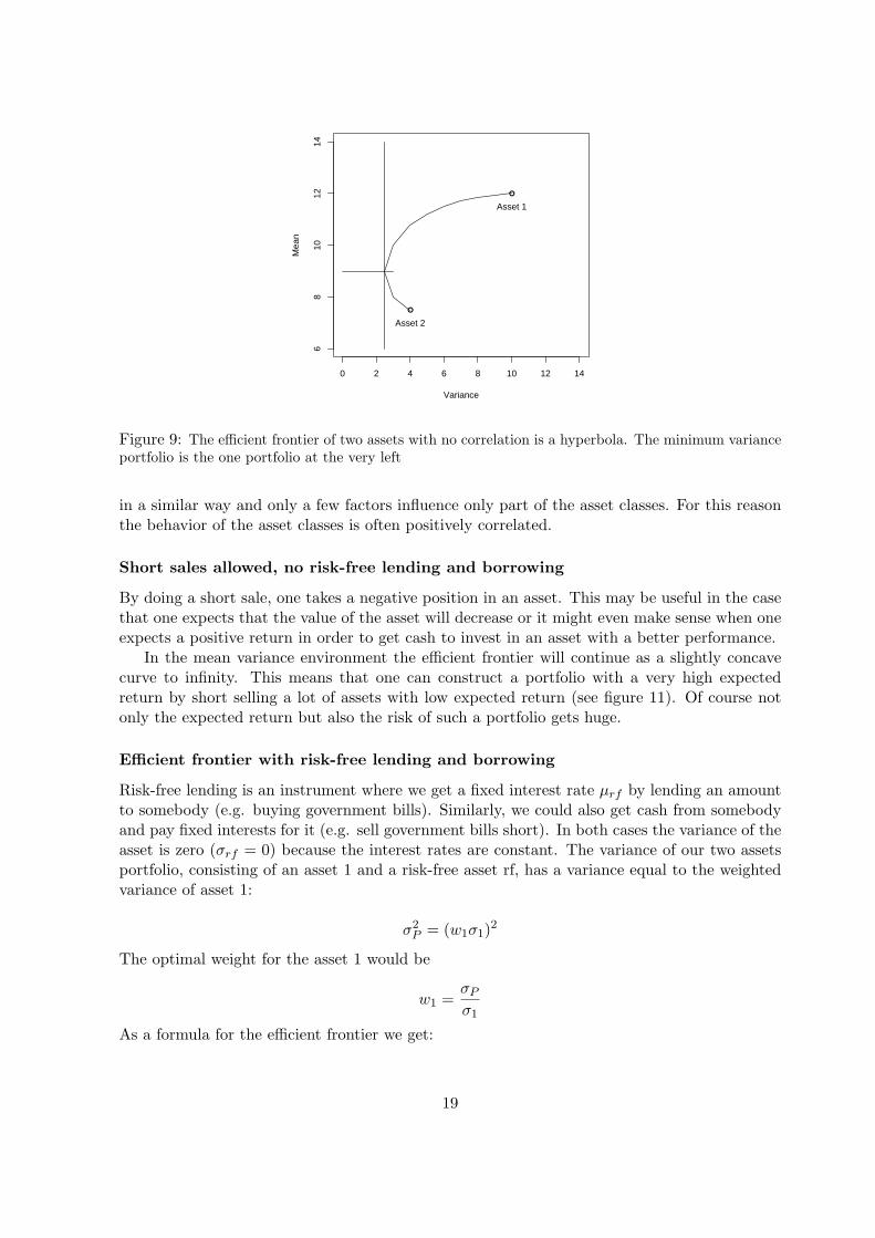
The efficient frontier and the minimum risk portfolio are shown in figure 9.

Intermediate risk In general we can say that the efficient frontier will be always to the leftof two assets, since the portfolio can be constructed as a linear combination of them. Figure 10shows that the efficient frontier moves to the left with decreasing correlation of the assets andallows a higher diversification and therefore a lower risk.

In practice we will find almost always positive correlation between asset classes and veryrarely a negative correlation. This means that there are only very few periods where a certainasset class has high profit and another asset class a negative profit. The reason lies in thefactors that influence the returns of the assets classes. Most factors influence all asset classes

18

0 2 4 6 8 10 12 14

68

1012

14

Variance

Mea

n

●

●

Asset 1

Asset 2

Figure 9: The efficient frontier of two assets with no correlation is a hyperbola. The minimum varianceportfolio is the one portfolio at the very left

in a similar way and only a few factors influence only part of the asset classes. For this reasonthe behavior of the asset classes is often positively correlated.

Short sales allowed, no risk-free lending and borrowing

By doing a short sale, one takes a negative position in an asset. This may be useful in the casethat one expects that the value of the asset will decrease or it might even make sense when oneexpects a positive return in order to get cash to invest in an asset with a better performance.

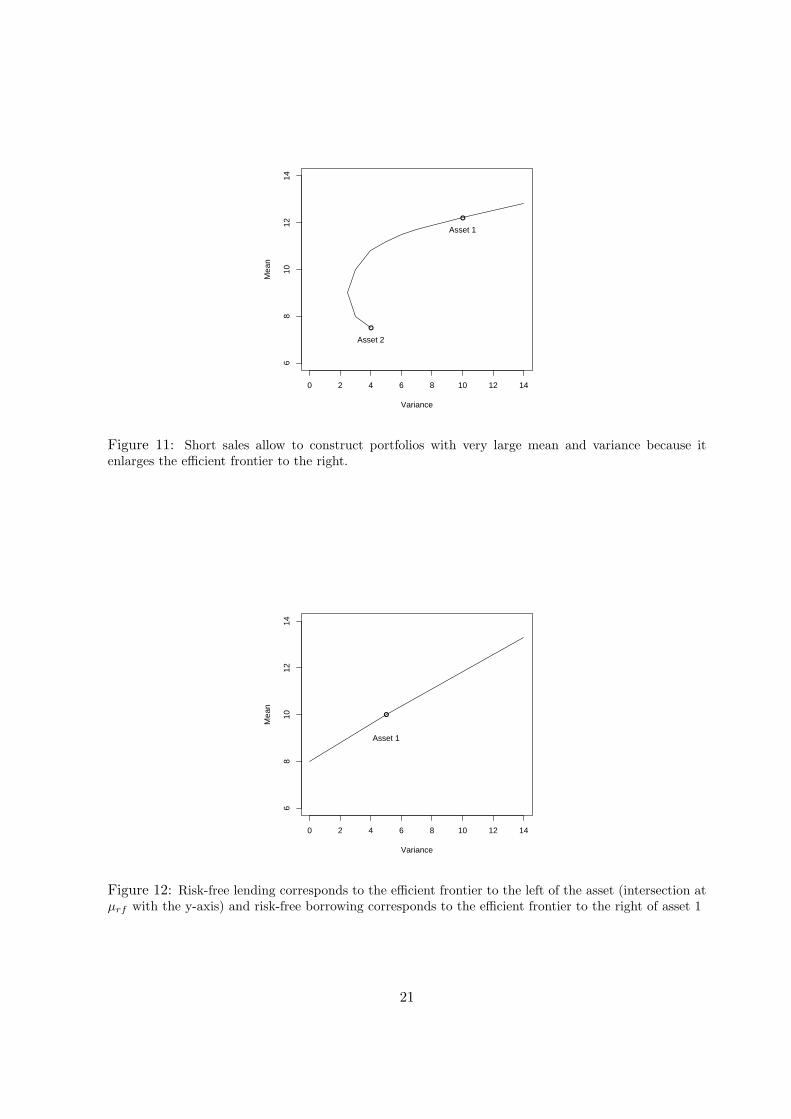
In the mean variance environment the efficient frontier will continue as a slightly concavecurve to infinity. This means that one can construct a portfolio with a very high expectedreturn by short selling a lot of assets with low expected return (see figure 11). Of course notonly the expected return but also the risk of such a portfolio gets huge.

Efficient frontier with risk-free lending and borrowing

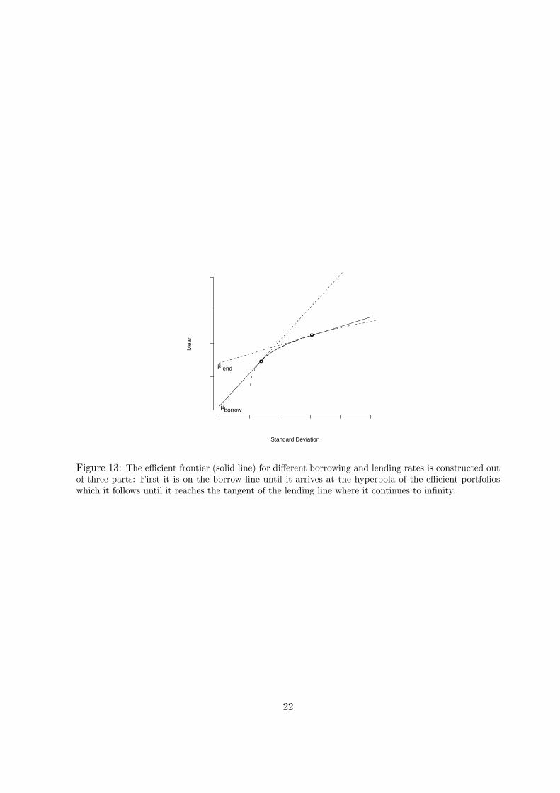
Risk-free lending is an instrument where we get a fixed interest rate µrf by lending an amountto somebody (e.g. buying government bills). Similarly, we could also get cash from somebodyand pay fixed interests for it (e.g. sell government bills short). In both cases the variance of theasset is zero (σrf = 0) because the interest rates are constant. The variance of our two assetsportfolio, consisting of an asset 1 and a risk-free asset rf, has a variance equal to the weightedvariance of asset 1:

σ2P = (w1σ1)2

The optimal weight for the asset 1 would be

w1 =σP

σ1

As a formula for the efficient frontier we get:

19

0 2 4 6 8 10 12 14

68

1012

14

Variance

Mea

n

●

●

●

Asset 1

Asset 2

Figure 10: Comparison of the efficient frontier of assets with different correlation. The correlation ofbetween asset 1 and asset 2 is -1, 0, 0.5, 1 (from left to right).

µP = (1− w1)µrf + w1µ1 =µ1 − µrf

σ1σP + µrf

From this term for the expected return of the portfolio we can see that the efficient frontieris again a linear curve as in figure 12. The term µ1−µrf

σ1or the slope of the function is called

leverage factor.To conclude, one can say that all portfolios constructed with risk-free lending and borrowing

lie on one straight line through the point (µrf ,0) and the point representing a portfolio consistingonly of the one available asset. By changing the leverage factor, one changes also µrf and σ2

P

in a linear way.As soon as risk-free lending and borrowing is possible, nobody will be interested anymore inthe hyperbola (and its expansion through short sales) described in the section above, but onlyin the tangent to the hyperbola through (µrf ,0) since it offers a higher µrf for a given σrf .

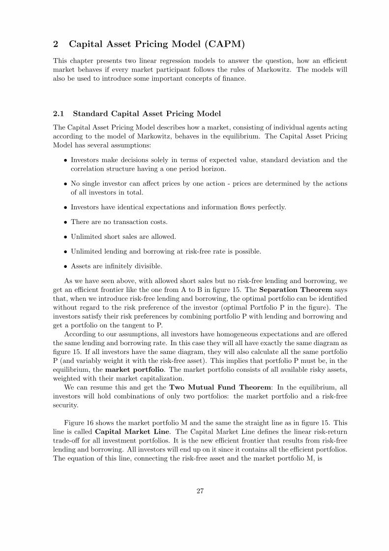
In the case that the lending rate is not the same as the borrowing rate, we get an efficientfrontier consisting out of three parts: It starts with the line of the borrowing rate until it touchesthe envelope of all the portfolio built without lending and borrowing and continues finally onthe line of the lending rate to infinity. Since short sales allow only a concave expansion of theefficient frontier to the right and the risk-free lending efficient frontier is a straight line, shortsales are also in this case of no interest anymore. An illustration is given in figure 13.

20

0 2 4 6 8 10 12 14

68

1012

14

Variance

Mea

n

●

●

Asset 1

Asset 2

Figure 11: Short sales allow to construct portfolios with very large mean and variance because itenlarges the efficient frontier to the right.

0 2 4 6 8 10 12 14

68

1012

14

Variance

Mea

n

●

Asset 1

Figure 12: Risk-free lending corresponds to the efficient frontier to the left of the asset (intersection atµrf with the y-axis) and risk-free borrowing corresponds to the efficient frontier to the right of asset 1

21

Standard Deviation

Mea

n

●

µborrow

●

µ lend

Figure 13: The efficient frontier (solid line) for different borrowing and lending rates is constructed outof three parts: First it is on the borrow line until it arrives at the hyperbola of the efficient portfolioswhich it follows until it reaches the tangent of the lending line where it continues to infinity.

22

Techniques for calculating the efficient frontier

In this chapter we will explain the techniques to determine the efficient frontier mathematically.Again, we will differentiate between the four cases of allowed and not allowed short sales andpossible and not possible risk-free lending and borrowing.

Short sales allowed, risk-free lending and borrowing possible

We start with the simplest case. From the earlier chapter we already know that with allowedshort sales and risk-free lending and borrowing there will be one optimal portfolio on the tangentfrom the risk-free asset (on the y-axis) to the envelope of all the efficient portfolios. The enabledrisk-free lending and borrowing makes this tangent to the efficient frontier. Our aim is for thisreason to maximize the slope of this tangent

θ =µ1 − µrf

σ1(14)

in order to maximize the return to risk ratio. There is a constraint to make sure that theweights add up to one

N∑i=1

wi = 1 (15)

With this setup we have a constraint maximization problem which could be solved with La-grangian multipliers. However it is possible to turn it into an unconstraint maximization prob-lem by combining the constraint (15) and the objective function (14). In order to do so, westart with:

µrf = 1µrf = (N∑

i=1

wi)µrf =N∑

i=1

wiµrf

Substituting this and our definition of the variance of a portfolio (2) into (14), we get

θ =∑N

i=1 wi(µi − µrf )√∑Ni=1 wiσi

2 +∑N

i=1

∑Nj=1 wiwjσij

The maximization problem can be solved by

∂θ

∂wi= 0

This gives us a system of equations where we can apply the following substitution

zi =µP − µrf

σ2P

wi

which leads to the following system of N simultaneous equations for N unknowns z1, . . . zN :

µ1 − µrf = z1σ21 + z2σ12 + . . . + zNσ1N

µ2 − µrf = z1σ12 + z2σ22 + . . . + zNσ2N

...µN − µrf = z1σ1N + z2σ2N + . . . + zNσ2

1N

23

The optimal weights wi can be received via

wi =wi∑N

i=112zi

Short sales allowed, risk-free lending and borrowing not possible

If there is no risk-free asset available, we can nevertheless assume that there is a risky freeasset with a specified return. Now we are in the case discussed before and can compute theoptimal portfolio corresponding to this situation. By changing the return of this fictive risk-freeasset to other rates, we can calculate the efficient frontier as the sum of the optimal portfolioscorresponding to different rates as shown in figure 14.

Standard Deviation

Mea

n

●

µrf1

●

µrf2

●

µrf3

Figure 14: In the case of allowed short sales but no risk-free assets, one can determine the efficientfrontier as sum of points corresponding to different (fictive) risk-free rates µrf1, µrf2, µrf3

Short sales not allowed, risk-free lending and borrowing possible

With the restriction of no short selling, we get an additional constraint and the optimizationproblem looks like

θ =µP − µrf

σP→ Max

subject to constraints

N∑i=1

wi = 1

wi ≥ 0,∀iThis last condition makes the problem hard to solve since we have a quadratic programmingproblem and no longer an analytical solution. The quadratic aspect is hidden in the objectivefunction: The σP -term contains squared terms in wi.To solve these kind of problems, one can use a standard solver package.

24

Short sales not allowed, risk-free lending and borrowing not possible

If the investor does not want to allow short sales and no risk-free asset is available, we can solvethe following optimization problem with the investors expected return µp

σ2P =

N∑i=1

(wiσi)2 +N∑

i=1

N∑j=1

wiwjσij → Min

subject to

N∑i=1

wi = 1

N∑i=1

wiµi = µP

wi ≥ 0,∀i

This is also a quadratic programming problem that should be solved with a computer package.

25

26

2 Capital Asset Pricing Model (CAPM)

This chapter presents two linear regression models to answer the question, how an efficientmarket behaves if every market participant follows the rules of Markowitz. The models willalso be used to introduce some important concepts of finance.

2.1 Standard Capital Asset Pricing Model

The Capital Asset Pricing Model describes how a market, consisting of individual agents actingaccording to the model of Markowitz, behaves in the equilibrium. The Capital Asset PricingModel has several assumptions:

• Investors make decisions solely in terms of expected value, standard deviation and thecorrelation structure having a one period horizon.

• No single investor can affect prices by one action - prices are determined by the actionsof all investors in total.

• Investors have identical expectations and information flows perfectly.

• There are no transaction costs.

• Unlimited short sales are allowed.

• Unlimited lending and borrowing at risk-free rate is possible.

• Assets are infinitely divisible.

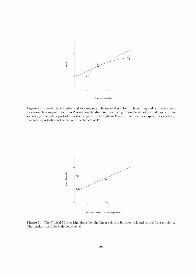
As we have seen above, with allowed short sales but no risk-free lending and borrowing, weget an efficient frontier like the one from A to B in figure 15. The Separation Theorem saysthat, when we introduce risk-free lending and borrowing, the optimal portfolio can be identifiedwithout regard to the risk preference of the investor (optimal Portfolio P in the figure). Theinvestors satisfy their risk preferences by combining portfolio P with lending and borrowing andget a portfolio on the tangent to P.

According to our assumptions, all investors have homogeneous expectations and are offeredthe same lending and borrowing rate. In this case they will all have exactly the same diagram asfigure 15. If all investors have the same diagram, they will also calculate all the same portfolioP (and variably weight it with the risk-free asset). This implies that portfolio P must be, in theequilibrium, the market portfolio. The market portfolio consists of all available risky assets,weighted with their market capitalization.

We can resume this and get the Two Mutual Fund Theorem: In the equilibrium, allinvestors will hold combinations of only two portfolios: the market portfolio and a risk-freesecurity.

Figure 16 shows the market portfolio M and the same the straight line as in figure 15. Thisline is called Capital Market Line. The Capital Market Line defines the linear risk-returntrade-off for all investment portfolios. It is the new efficient frontier that results from risk-freelending and borrowing. All investors will end up on it since it contains all the efficient portfolios.The equation of this line, connecting the risk-free asset and the market portfolio M, is

27

Standard Deviation

Mea

n

●

●

A

B

P

rf

Figure 15: The efficient frontier and its tangent at the optimal portfolio. By lending and borrowing, onemoves on the tangent: Portfolio P is without lending and borrowing. If one lends additional capital fromsomebody, one gets a portfolio on the tangent to the right of P and if one borrows capital to somebodyone gets a portfolio on the tangent to the left of P.

Standard Deviation of efficient portfolio

Mea

n of

por

tfolio

M

µM

σM

µrf

Figure 16: The Capital Market Line describes the linear relation between risk and return for a portfolio.The market portfolio is depicted as M

28

Variance between market and individual asset

Mea

n in

divi

dual

ass

et

M

µM

σM2

µrf

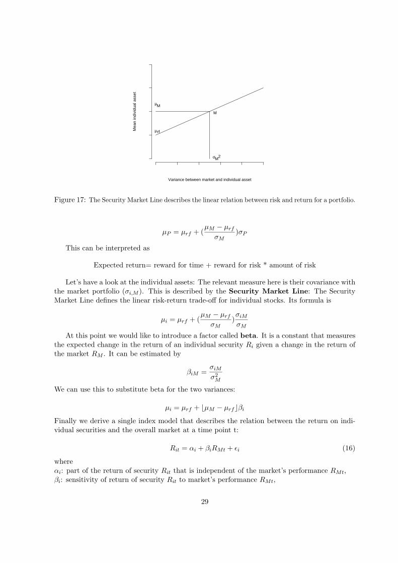
Figure 17: The Security Market Line describes the linear relation between risk and return for a portfolio.

µP = µrf + (µM − µrf

σM)σP

This can be interpreted as

Expected return= reward for time + reward for risk * amount of risk

Let’s have a look at the individual assets: The relevant measure here is their covariance withthe market portfolio (σi,M ). This is described by the Security Market Line: The SecurityMarket Line defines the linear risk-return trade-off for individual stocks. Its formula is

µi = µrf + (µM − µrf

σM)σiM

σM

At this point we would like to introduce a factor called beta. It is a constant that measuresthe expected change in the return of an individual security Ri given a change in the return ofthe market RM . It can be estimated by

βiM =σiM

σ2M

We can use this to substitute beta for the two variances:

µi = µrf + bµM − µrfcβi

Finally we derive a single index model that describes the relation between the return on indi-vidual securities and the overall market at a time point t:

Rit = αi + βiRMt + εi (16)

whereαi: part of the return of security Rit that is independent of the market’s performance RMt,βi: sensitivity of return of security Rit to market’s performance RMt,

29

RMt: return of the market,εi : a random error term with mean equal to zero.

Beta measures how sensitive a stock’s return is to the return of the market. A beta of twomeans that the return of the stock will be the double of the return of the market (no matterwhether it is a loss or a gain). Similarly, a beta of 0.5 means that the stock will move only halfas much as the market does. In other words, a stock with a high beta gets a high risk premiumand a stock with a low beta gets a low risk premium.The intention of splitting the return of a stock into a part that is related to the market (βiRMt)and a part that is related to the individual stock (αi) comes from the observation, that whenthe market goes up, most stocks follow this trend and vice versa. Therefore is a part of thestock return related to the market return. It is interesting in (16) to see that the return isonly influenced by the market risk and investors don’t receive a premia for holding additionaldiversifiable/non market risk.

We can summarize that the Capital Asset Pricing Model is a theoretical model to identifythe tangency portfolio. It uses some ideal assumptions about the economy to conclude that thecapital weighted world wealth portfolio it the tangency portfolio and that every investor willhold this portfolio.

2.2 Arbitrage Pricing Theory (APT)

The Arbitrage Pricing theory is an alternative approach to determining asset prices. It was firstintroduced in [37] and bases on the idea that exactly the same instrument can not be differentlypriced.

As we have seen, the Capital Asset Pricing Model has some quite restrictive assumptions.This gives space for the Arbitrage Pricing Theory. It asks for the following conditions to befulfilled

• Returns are generated according to a linear factor model.

• The number of assets N is close to infinite.

• Investors have homogenous expectations (same as in CAPM).

• Capital markets are perfect (perfect competition, no transaction costs - same as CAPM).

The Arbitrage Pricing Theory states that returns of stocks are generated by a linear modelconsisting of F factors Ij

Ri = ai + bi1I1 + bi2I2 + . . . + biF IF + ei (17)

whereai : the expected return for stock i if all factors have a value of zero,Ij : the value of factor j that impacts the return on stock i,bij : the sensitivity of stock i’s return to factor j,ei : a random error term with mean equal to zero and variance equal to σ2

ei. This error is

uncorrelated with the factors bij and errors of the other assets (unsystematic risk).

30

If the assumptions hold, we can combine the assets to get a risk-free portfolio that requireszero net investment (i.e. by short selling certain assets and buying others with the revenue).The fundamental implication of the Arbitrage Pricing Theory is that such a free, risk-free port-folio (arbitrage portfolio) must have a zero return on the average. This is intuitive since arisk-free portfolio with an expected return of non zero is an arbitrage opportunity which wouldbe exploited immediately by market participants and hence diminish.

Let’s express this in a more mathematical way: Using (17) we can write the expectedportfolio return as

µP =N∑

i=1

wiai +N∑

i=1

wibi1I1 + . . . +N∑

i=1

wibiF IF +N∑

i=1

wiei (18)

We have assumed that the number of stocks are close to infinite. So, it is possible to find aportfolio that satisfies the following properties:

N∑i=1

wi = 0

N∑i=1

wiai = 0

N∑i=1

wibi1 = 0

N∑i=1

wibi2 = 0

...N∑

i=1

wibiF = 0

The first condition defines that we have no net investment since we want an arbitrage portfolio.The second condition asks the expected return for this stock to be zero if all factors are set tozero (non-arbitrage condition). The following conditions imply that the portfolio has no risksince it has no exposure to any of its constituents. These three types of conditions are calledorthogonality constraints. Applying them to (18), we can see that it must produce an expectedreturn of zero. Again, if this would not hold true, investors would have a free money generator.

It shows that the orthogonality constraints imply that the expected returns µRi are a linearcombination of the bij and a constant. This means that there exists a set of factors λ0 . . . λF

such that

µRi = λ0 + λ1bi1 + . . . + λF biF

The bij can still be interpreted as the sensitivity of the assets to a change in an underlyingfactor Ii. In contrast, the λj represent the risk premia of the respective factor.

We are determining now the λj by using the fact that an asset with single exposure to onefactor and no exposure to the other factors has the same risk premia as this factor. For each

31

λj , j = 1 . . . F we do the following: The respective bij is set to 1 and all the other equal to 0.With this procedure we find that

µRi = λ0 + bi1(µR1 − λ0) + . . . + biF (µRF− λ0)

We assume that for i = 0 we have the risk-free asset since the risk-free asset does not dependon any other factors (b0j = 0, j = 1 . . . F ). For this special case of the APT model we get

µR0 = λ0 = µrf

and therefore we can express the model as formula for the excess return

µRi − µrf = bi1(µR1 − µrf ) + . . . + biF (µRF− µrf )

The Capital Asset Pricing Model can be seen as a very special case of the Arbitrage PricingModel with only one factor (single index model). This can be shown if one sets F = 1. Thenwe have left

Ri = ai + bi1I1 + ei

Now we can interpret ai as the return of the risk-free asset µrf and bi1I1 as the return of themarket portfolio RM times the leverage factor.

Ri = µrf + b1RMi + ei

And this is the same expression as (16) for the CAPM.

Factor analysis is the principal methodology used to estimate the factors Ij and factorloadings bij . Since it is not possible to calculate a perfect specification of the model describedby (17), a factor analysis will derive a good approximation. The criteria for the goodness isthe covariance of residual returns which should be minimal. To execute a factor analysis, onehas to determine the number of desired factors in advance. By repeating this process for anincreasing number of factors, one gets one solution for each number of factors. A criteria tostop increasing the number of factors would be, if the probability that the next factor explainsa statistically significant portion of the covariance drops below some level (e.g. 50%).

There are factor analysis methods that produce orthogonal factors (e.g. principal compo-nent analysis) and others that produce non-orthogonal factors. It may become a disadvantageto choose a method that creates orthogonal factors since the factors it creates do not exist in thereal world and can therefore not be interpreted. However they can be used in a pure statisticalmodel by assuming that the past data will be valid for the next step and applying them tocalculate one step into the future. The non-orthogonal model might be not so accurate, but assoon as one gets the factors (like indices or interest rates) and their respective weights, one canapply the model in the future with new data from these factors.

To conclude, we can say that the Arbitrage Pricing Model has a number of benefits: It is notas restrictive as the Capital Asset Pricing Model in its requirement concerning the distributionof the returns and the investors utility function. It also allows multiple sources of risk to explainthe stock return movements. Further it avoids using the concept of a Market portfolio. This isan advantage because this concept is hard to observe in practice.

The flexibility is also the main disadvantage of the model: The investors have to decidewhich sources of risk they want to include and how to weight them. Further the APT modelmight not be so intuitive as the CAPM.

32

Nevertheless, the Arbitrage Pricing Theory remains the newest and a promising explanationof relative returns.

33

Part II

Beyond Markowitz

We have seen in the first part that the approach to optimize a portfolio as proposed byMarkowitz asks for some strong assumptions like normal distributed returns. In this secondpart we will investigate whether it can be assumed that the returns of financial assets areproduced by a normal distribution. As we will seen, there will be several aspects that indicatethat this assumption does not hold. We will use this as justification for analyzing furtherportfolio optimization algorithms that do not have such a strong requirement to the underlyingdistribution function of the asset returns.

3 Stylized Facts Of Asset Returns

In this chapter we will present some statistical tests to investigate the characteristic propertiesof financial market data. The used tests are chosen with respect to the properties that are im-portant specially for financial time series. The tests for determining the form of the underlyingdistribution function that has created the returns are Goodness of fit (Kolmogorov-Smirnovtest), Kurtosis and Skewness (Jarque-Bera test) and Quantile-Quantile plots. Concerning theform of the distribution function, we especially test for the Normal distribution. Further wehave selected two tests for detecting dependencies and long memory effects in the time series.These are the Runs test for randomness and BDS test for dependencies.The focus of the tests as a whole lies on the detection of fat tail behavior rather than de-pendencies. The tests are presented in their functionality and demonstrated on representative,artificial data. In part III of the thesis the tests are applied to real market data and the resultingconclusions drawn.

Non normality in return distributions

A very important question in financial analysis is the one for the distribution function of theasset returns. Since a lot of methods and theorems are assuming a certain distribution function,it is crucial to analyze the origin of the returns.There are two aspects of the distribution function that has created the asset returns that shouldbe considered:

• Form: Does the distribution have fat tails or skewness?

• Dependencies: Do the returns depend on an earlier return values?

The normal distribution was first mentioned by de Moivre in 1733 [31]. The advantages of thisdistribution are

• It can be defined by only two variables: mean and variance.

• It describes random behavior in a natural mechanisms.

34

For this reasons and the fact that it is possible to fit it as a first approximation to asset returns,the normal distribution is used a lot in financial analysis and is still considered as the standardassumption.However, in 1963 Mandelbrot [29] observed that financial returns might not be produced by anormal distribution.

3.1 Distribution Form Tests

Goodness of fit test (Kolmogorov-Smirnov test)

We start with the Kolmogorov-Smirnov one-sample test which can be used to answer the ques-tion, whether a sample comes from a population with a specific distribution. The test is basedon the empirical distribution function of the given samples and is restricted to continuous dis-tributions to test for.Assuming we are given the samples as X1, X2, . . . , XN . We can order them and calculate theempirical distribution function as

EN =n(i)N

with n(i) as the number of samples that are smaller than Xi. The Kolmogorov-Smirnov testdetermines the maximum distance between this empirical distribution function and the cumu-lative distribution function of the assumed underlying function. Figure 18 shows a chart withthese two distribution functions.

−0.05 0.00 0.05

0.0

0.2

0.4

0.6

0.8

1.0

X

Cum

ulat

ive

Pro

babi

lity

Figure 18: The Kolmogorov-Smirnov test calculates the maximum difference between the empiricaldistribution function of the samples (doted line) and the cumulative distribution function of the assumedunderlying function (solid line).

The hypothesis of the test are defined as:Null hypothesis: The data follows the assumed distribution

35

Alternative hypothesis: The data does not follow the assumed distributionThe precise test statistic is

D = maxi≤i≤N

|F (Xi)−i

N|

with F (Xi) as the assumed underlying distribution function. The null hypothesis of the dis-tribution is rejected if

√NDN , dependent on the confidence level, is greater than the critical

value derived from the standard normal distribution.There are two equivalent ways to handle the underlying distribution. In both ways the mean

µ and variance σ of the underlying distribution need to be estimated out of the given samples.It is then possible to compare the samples to a normal distribution with the estimated mean µand variance σ. Otherwise one can transform the given samples according to

Xi =Xi − µ

σ(19)

and compare the new samples to a standard normal distribution.

Some points classify the Kolmogorov-Smirnov test as unsatisfiable for our purpose: First,since the test compares the absolute difference between the two cumulative distributions, itunderweights the difference in the tails and overweights the difference near the mean of thedistribution. However we want especially check whether our distribution has fat tails. Thesecond disadvantage of the Kolmogorov-Smirnov test is that it is a very general method (it canalso be used for comparing with other distributions than just the normal) and is thus takingonly the mean and variance of a distribution into consideration.

Skewness and kurtosis (Jarque-Bera test)

For the Kolmogorov-Smirnov test we were looking at the first and second moment of the dis-tribution.

µ =∑

i

wixi

σ2 =∑

i

wi(xi − µ)2

In terms of the normal distribution, often the third and fourth moments become interesting.Skewness is the standardized third moment

ς =∑

i wi(xi − µ)3

σ3

Skewness can be interpreted as a measure for the asymmetry of a distribution function wherebya value of 0 indicates absolute symmetry (e.g. the normal distribution), a positive skewnessmeans an increased probability at the higher quantiles (heavy right tail) and a negative skewnesssays that we have an increased probability at the lower quantiles (heavy left tail). Figure 19shows some examples of empirical distributions with skewness.

The standardized fourth moment is called kurtosis. Because the normal distribution has akurtosis of 3, one often calculates the excess kurtosis which is the kurtosis minus 3.

κ =∑

i wi(xi − µ)4

σ4− 3

36

−4 −2 0 2 4

0.0

0.1

0.2

0.3

0.4

0.5

0.6

X

Prob

abilit

y

−4 −2 0 2 4

0.0

0.1

0.2

0.3

0.4

0.5

X

Prob

abilit

y

Figure 19: The charts show skewed normal distributions (solid) in comparison with a normal distribution(doted). The left chart is drawn by a standard normal distribution with a shape parameter of -3, whilethe right chart is drawn by a standard normal distribution with shape parameter of 1.

The kurtosis of a distribution defines whether the distribution has fat tails in comparison witha normal distribution or not. The following holds true for most financial time series: A negativekurtosis indicates that both tails are less pronounced and the distribution is less peaked as anormal distribution (platykurtic). A distribution with a kurtosis of 0 is called mesokurtic. Theopposite of platykurtic, a positive kurtosis, means fat tails and more peakedness than a normaldistribution (leptokurtic). If there is excess kurtosis, the mid-range values on both sides of themean have less weight than in a normal distribution. This means that distributions with a highkurtosis are appropriate when the returns are likely to be very small or are likely to be verylarge but are not very likely to have values between these two extremes.

−10 −5 0 5 10

0.00

0.05

0.10

0.15

0.20

0.25

0.30

0.35

X

Prob

abilit

y

−4 −2 0 2 4

−5−4

−3−2

−1

X

log(

Prob

abilit

y(X)

)

Figure 20: The charts show a Student-t distribution with an excess kurtosis of 6.7 (solid) in comparisonwith a normal distribution (doted). The left chart uses a linear y-axis whereby the right chart uses alogarithmic y-axis to make the excess kurtosis more explicitly. In the log chart appear the the fat tailsof the student distribution as a line above the tails of the normal distribution.

With these definitions, the normal distribution has a skewness and a kurtosis of 0. TheJarque-Bera test calculates the skewness and kurtosis of a given distribution to find out, whetherit is a normal distribution (with a value of 0 for both) or not. The test statistics is as follows:

37

If we assume normality for the underlying distribution, the standard error for the estimated

skewness ς and kurtosis κ are approximately√

6N and

√24N with N as the sample size. The

Jarque-Bera test is defined as

JB = N [(ς2

6) + (

κ2

24)] (20)

and is asymptotically chi-squared with 2 degrees of freedom.

Quantile-Quantile plot

In this section we would like to present a graphical method to assign some sample data to apossible distribution. An α quantiles is defined as x such that

P [X < x] = α

The quantile-quantile plot (QQ plot) is a scatter plot with the quantiles of the given empiricaldistribution on the vertical axis and the quantiles of the theoretical distribution on the horizontalaxis. In order to calculate the quantiles of the empirical distribution, one first has to transformthe empirical distribution according to the standard normal transformation (19). Now onecan draw the QQ plot as scatter plot of the transformed empirical and the standard normalquantiles.

In [19] the main merits of a QQ plot are described as:

• If a random sample set is compared to its own distribution, the plot should look roughlylinear.

• If there are a few outliers contained in the data, it is possible to identify them by lookingat the scatter plot.

• If one distribution is transformed by a linear function, this transforms the QQ plot by thesame linear transformation. The transformation can be estimated from the plot (slopeand intercept)

• It is possible to deduce small differences in the participating distributions from the plot(e.g. fat tails imply curves at the left and right end)

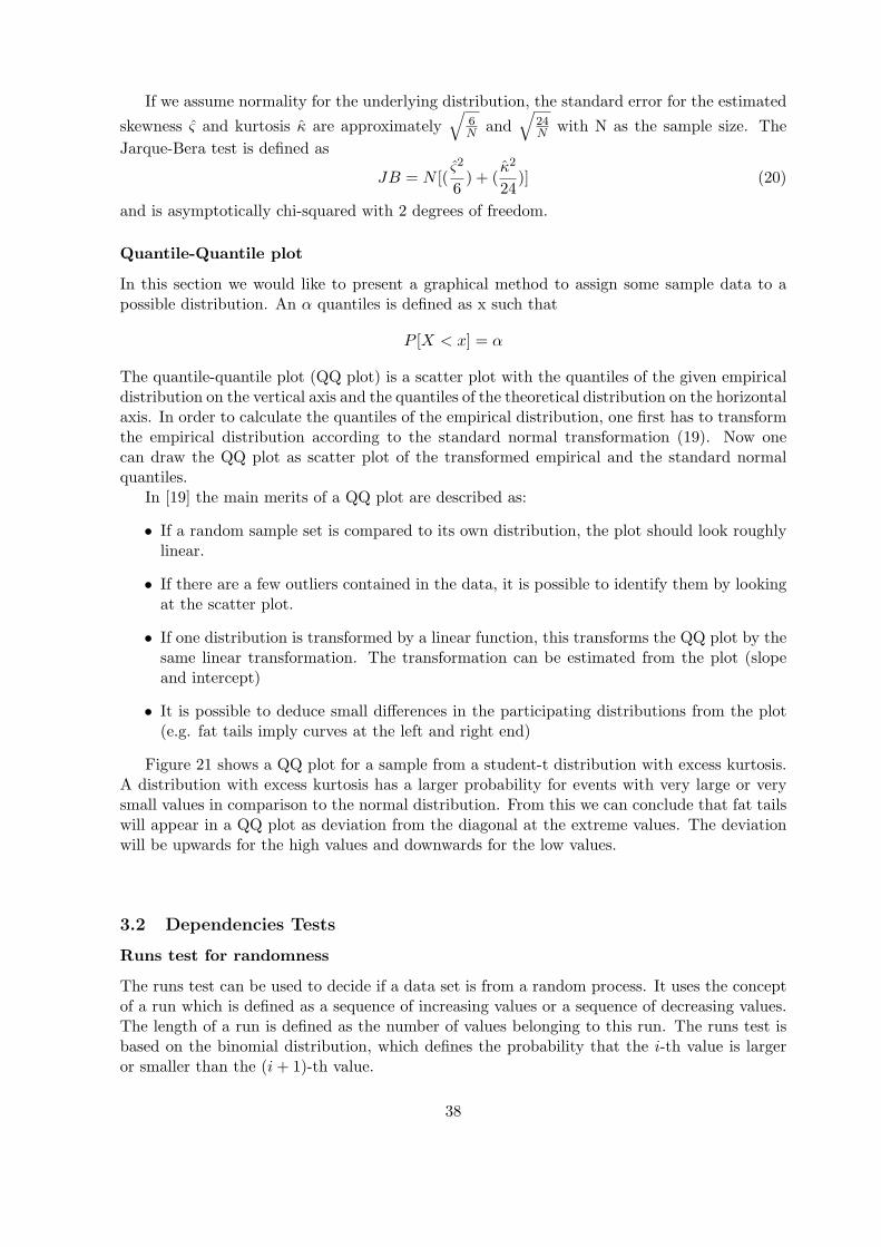
Figure 21 shows a QQ plot for a sample from a student-t distribution with excess kurtosis.A distribution with excess kurtosis has a larger probability for events with very large or verysmall values in comparison to the normal distribution. From this we can conclude that fat tailswill appear in a QQ plot as deviation from the diagonal at the extreme values. The deviationwill be upwards for the high values and downwards for the low values.

3.2 Dependencies Tests

Runs test for randomness

The runs test can be used to decide if a data set is from a random process. It uses the conceptof a run which is defined as a sequence of increasing values or a sequence of decreasing values.The length of a run is defined as the number of values belonging to this run. The runs test isbased on the binomial distribution, which defines the probability that the i-th value is largeror smaller than the (i + 1)-th value.

38

●

●

●

●

●

●

●●

●●●●

●

●

●

●

●●

●

●

●

●

●●

●

●

●

●

●

●

●

●

●●●

●

●

●

●

●

●

●●

●

●

●

●

●

●

●

●

●

●

●

●

●

●

●

●

●

●

●

●

●

●

●

●●

●

●

●

●●

●●●

●

●●

●

●

●●

●

●

●

●

●

●

●

●

●

●

●

●

●●

●

●

●

●

●●

●

●●

●●

●●

● ●

●●

●

●

●

●

●

●

●●

●

●

●

●

●

●

●

●●

●

●

●

●

●

●

●

●

●

●

●

●

●

●

●

●

●●●

●

●●

●

●●

●

●

●

●

●

●

●

●

●●

●

●●●

●

●

●

●●

●

●●●

●

●

●●

●

●

●

●

●

●

●

●●

●

●

●

●

●

●

●

●

●

●●●

●

●

●

●

●

●

●

●

●

●●

●

●● ●

●

●

●●

●●

●

●

●

●

●

●●

●

●

●

●

●

●

●

●

●

●

●●

●

●

●

●

●

●●

●

●●

●

●

●

●

●

●

●

●●

●

●

●

●

●●

●

●

●

●●●

●

●

●

●

●

●

●●

●

●

●

●

●

●

●

●

●

●

●

●●

●

●

●

●

●

●

●●

●

●

●

●●

●●

●

●

●

●

●

●

●

●●

●

●

●

●●

●●

●

●●

●●

●●●

●

●

●

●

●

●●

●●

●

●

●

●

●

●

●

●

●

●

●

●

●

●

●

●●

●●

●

●●

●

●●●●

●●

●

●●

●

●

●

●

●●

●

●

●

●

●

●

●

●●

●

●

●●

●

●●

●

●

●

●

●

●

●

●●

●

●

●

●

●

●●

●●

●

●

●

●

●

●

●

●●●

●

●

●

●

●

●

●

●

●

●

●●

●

●

●●

●

●●●

●●

●

●

●

●●●

●

●●

●●

●

●

●

●

●●

●

●

●●●

●

●

●●

●●

●

●

●

●

●

●

●

●

●

●●

●

●

●

●●

●

●●

●

●

●

●

●

●

●

●

●

●●

●

●

●

●

●

●●

●

●

●

●

●

●

●●

●

●

●

●

●

●

●

●

●

●

●

●●

●

●

●

●●

●

●●

●

●

●●

●

●

●

●●●

●

●

●

●

●

●

●

●

●

●

●

●

●

●●

●

●

●

●

●

●

●

●

●●

●

●●

●

●

●

●

●

●

●

●

●

●●

●

●

●

●

●

●

●

●

●

●

●●

●

●

●

●

●●

●

●●

●

●

●

●

●

●

●

●

●

●

●

●

●

●

●●

●

●

●

●

●

●

●●●

●

●

●

●

●

●

●●

●

●

●

●

●

●

●

●

●

●

●●

●

●

●●

●

●

●

●

●

●

●

●●

●

●

●

●

●●

●

●

●

●

●●●

●

●

●

●

●●

●

●

●

●

●

●

●

●●

●●

●

●

●●

●●

●

●

●●

●

●

●

●

●

●

●

●

●

●●

●

●

●

●

●●

●

●

●

●

●

●

●●

●

●●

●

●

●

●●

●

●

●

●

●

●

●

●

●

●

●

●

●●

●

●

●

●

●

●●

●

●

●

●

●

●

●

●

●

●

●

●

●●

●●

●

●●●

●

●

●

●

●

●

●●

●●

●

●

●

●

●

●

●

●

●

●

●

●

●

●

●

●

●

●

●

●

●

●

●

●

●

●

●●

●

●

●

●

●●

●

●

●

●

●●

●

●

●

●

●

●

●

●

●

●

●

●

●

●●

●

●

●

●

●

●

●●

●

●

●

●●

●

●

●

●

●

●

●

●

●●●

●

●●

●

●

●

●

●

●

●

●

●

●●

●

●

●

●

●

●

●

●●

●

●

●

●

●●

●

●

●

●

●

●

●

●

●●

●

●

● ●

●

●

●

●

●

●●

●●

●

●

●●●

●●

●

●

●

●

●

●

●●●

●

●●●

●

●

●

●

●

●

●●

●

●

●

●

●

●

●●

●●

●

●

●●

●

●

●

●

●

●

●

●

●

●

●

●

●

●●●●

●

●●

●

●

●

●●

●

●

●

●

●

●

●

●

−3 −2 −1 0 1 2 3

−8−6

−4−2

02

46

Normal QQ−Plot

Normal Quantiles

Stud

ent−

t Qua

ntile

s

●

●

●●●●●●

●●●●●

●●●●●●●

●●●●●●●●●●●

●●●●●●●●●●●●●●●●●●

●●●●●●●●●●●●●●●●●●●●●●●●●●●

●●●●●●●●●●●●●●●●●●●●●●●●●●●●●●●●●●●●●●●●●●●

●●●●●●●●●●●●●●●●●●●●●●●●●●●●●●●●●●●●●●●●●●●●●●●●●●●●●●●●●●●●●●●●●●●

●●●●●●●●●●●●●●●●●●●●●●●●●●●●●●●●●●●●●●●●●●●●●●●●●●●●●●●●●●●●●●●●●●●●●●●●●●●●●●●●●●●●●●●●●●●●●●●●

●●●●●●●●●●●●●●●●●●●●●●●●●●●●●●●●●●●●●●●●●●●●●●●●●●●●●●●●●●●●●●●●●●●●●●●●●●●●●●●●●●●●●●●●●●●●●●●●●●●●●●●●●●●●●●●●●●●●●●●●●●●●

●●●●●●●●●●●●●●●●●●●●●●●●●●●●●●●●●●●●●●●●●●●●●●●●●●●●●●●●●●●●●●●●●●●●●●●●●●●●●●●●●●●●●●●●●●●●●●●●●●●●●●●●●●●●●●●●●●●●●●●●●●●●●●●●●●●●●●●●●●●

●●●●●●●●●●●●●●●●●●●●●●●●●●●●●●●●●●●●●●●●●●●●●●●●●●●●●●●●●●●●●●●●●●●●●●●●●●●●●●●●●●●●●●●●●●●●●●●●●●●●●●●●●●●●●●●●●●●●●●●●●●●●●●●●●●●●

●●●●●●●●●●●●●●●●●●●●●●●●●●●●●●●●●●●●●●●●●●●●●●●●●●●●●●●●●●●●●●●●●●●●●●●●●●●●●●●●●●●●●●●●●●●●●●●●●●●●●●●●●●●

●●●●●●●●●●●●●●●●●●●●●●●●●●●●●●●●●●●●●●●●●●●●●●●●●●●●●●●●●●●●●●●●●●●●●●●●●●●●

●●●●●●●●●●●●●●●●●●●●●●●●●●●●●●●●●●●●●●●●●●●●●●●●●●

●●●●●●●●●●●●●●●●●●●●●●●●●●●●●●●●

●●●●●●●●●●●●●●●●●●●●

●●●●●●●●●●●●●

●●●●●●●●●

●●●●●●●

●●●●●

●

●

●

−3 −2 −1 0 1 2 3

−6−4

−20

24

6

Normal QQ−Plot

Normal Quantiles

Stud

ent−

t Qua

ntile

s

Figure 21: The charts show QQ plots for a student-t distribution with a degree of freedom of 4 incomparison with the normal distribution. The left chart was created from a sample set of 1000 elementsfrom the student-t distribution and the right chart directly from the quantiles of the same normal andstudent-t distribution. The right chart is therefore smoother. The fat tails of the student distributionappear in both charts as deviation from the diagonal.

For the test we have to calculate the ni’s, the number of runs of length i for 1 ≤ i ≤ 10. We canthen normalize the ni’s with the expected number of runs of length i (µni) and the standarddeviation of the number of runs of length i (σni). These values µni and σni can be receivedfrom the binomial distribution.The final test value is the normalized ni:

zi =ni − µni

σni

which is compared to the two sided standard normal table. A zi value greater than the table en-try indicates non-randomness. Figure 22 and 23 show some outcome of AR(1) and GARCH(1,1)processes with the corresponding test results.

BDS test for dependencies

The BDS test is a non-parametric method of testing for nonlinear patterns in time series. Itwas first developed by Brock, Dechert and Scheinkman in 1987 (see [11]). The test has the nullhypothesis that the data in the time series is independently and identically distributed (iid)and is in [8] defined as

BT =√

T −m + 1(CT (m, ε)− CT (1, ε)m)σ(m, ε)

where

• CT (m, ε) is the correlation integral defined by

CT (mε) = (T−m2 )−1

∑∀s<t

Iε(Y mt , Y m

s )

• Y mt = (yt, yt+1, · · · , yt+m−1) is the m-history of yt

39

Time

x

0 200 400 600 800 1000

−2

02

Time

x

0 200 400 600 800 1000

−5

05

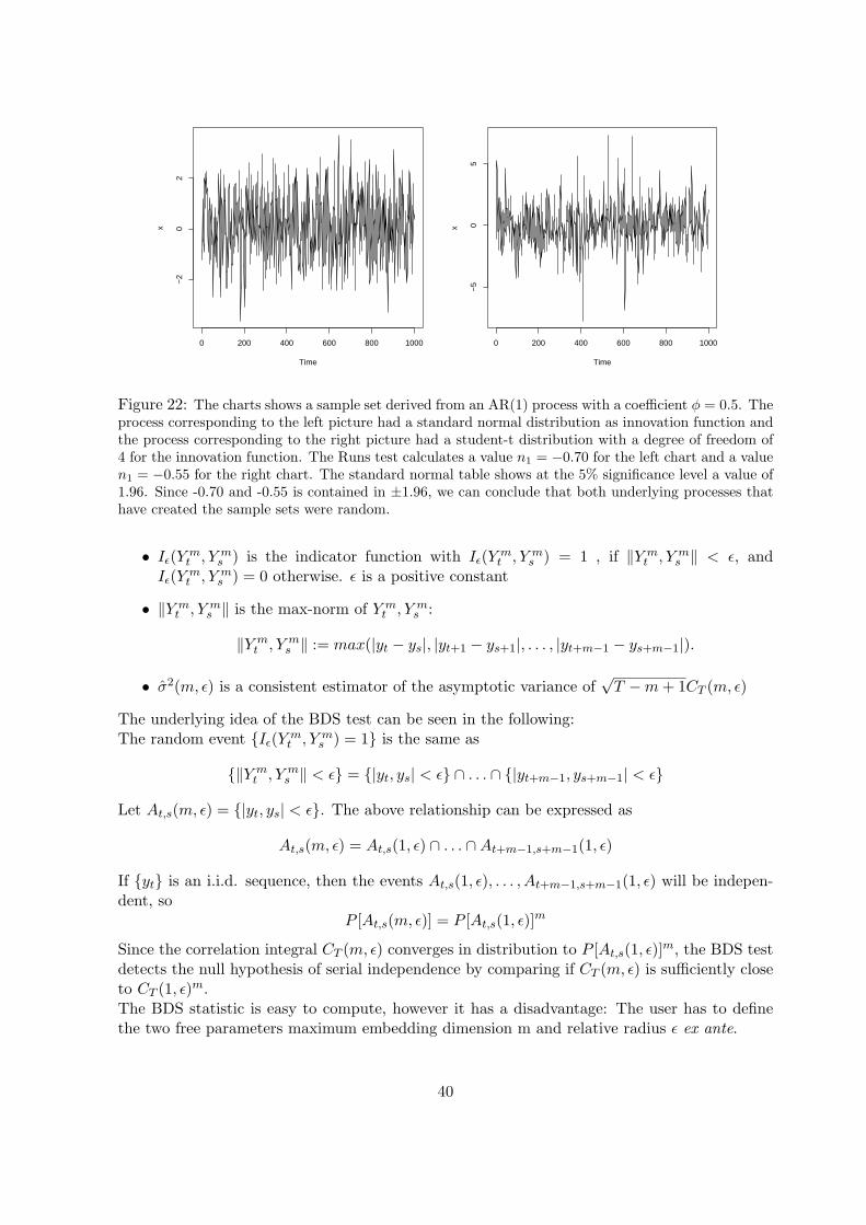
Figure 22: The charts shows a sample set derived from an AR(1) process with a coefficient φ = 0.5. Theprocess corresponding to the left picture had a standard normal distribution as innovation function andthe process corresponding to the right picture had a student-t distribution with a degree of freedom of4 for the innovation function. The Runs test calculates a value n1 = −0.70 for the left chart and a valuen1 = −0.55 for the right chart. The standard normal table shows at the 5% significance level a value of1.96. Since -0.70 and -0.55 is contained in ±1.96, we can conclude that both underlying processes thathave created the sample sets were random.

• Iε(Y mt , Y m

s ) is the indicator function with Iε(Y mt , Y m

s ) = 1 , if ‖Y mt , Y m

s ‖ < ε, andIε(Y m

t , Y ms ) = 0 otherwise. ε is a positive constant

• ‖Y mt , Y m

s ‖ is the max-norm of Y mt , Y m

s :

‖Y mt , Y m

s ‖ := max(|yt − ys|, |yt+1 − ys+1|, . . . , |yt+m−1 − ys+m−1|).

• σ2(m, ε) is a consistent estimator of the asymptotic variance of√

T −m + 1CT (m, ε)

The underlying idea of the BDS test can be seen in the following:The random event {Iε(Y m

t , Y ms ) = 1} is the same as

{‖Y mt , Y m

s ‖ < ε} = {|yt, ys| < ε} ∩ . . . ∩ {|yt+m−1, ys+m−1| < ε}

Let At,s(m, ε) = {|yt, ys| < ε}. The above relationship can be expressed as

At,s(m, ε) = At,s(1, ε) ∩ . . . ∩At+m−1,s+m−1(1, ε)

If {yt} is an i.i.d. sequence, then the events At,s(1, ε), . . . , At+m−1,s+m−1(1, ε) will be indepen-dent, so

P [At,s(m, ε)] = P [At,s(1, ε)]m

Since the correlation integral CT (m, ε) converges in distribution to P [At,s(1, ε)]m, the BDS testdetects the null hypothesis of serial independence by comparing if CT (m, ε) is sufficiently closeto CT (1, ε)m.The BDS statistic is easy to compute, however it has a disadvantage: The user has to definethe two free parameters maximum embedding dimension m and relative radius ε ex ante.

40

0 200 400 600 800 1000

−0.

010

−0.

005

0.00

00.

005

0.01

0

Index

x

0 200 400 600 800 1000

−0.

06−

0.04

−0.

020.

000.

020.

04

Index

x

Figure 23: The charts show the same calculations as in figure 22 with an GARCH process (as described in[10]) as underlying function. Again, the process corresponding to the left picture had a standard normaldistribution as innovation function and the process corresponding to the right picture had a student-tdistribution with a degree of freedom of 4 for the innovation function. The Runs test calculates a valuen1 = −0.65 for the left chart and a value n1 = −0.62 for the right chart. So we can again conclude thatboth underlying processes that have created the sample sets were random.

We will use the same AR(1) and GARCH(1,1) processes as described in figure 22 and 23for the Runs test and apply the BDS test to them. The following part shows the detailed BDSanalysis for the AR(1) process with normal innovation:

Embedding dimension = 2, 3Epsilon for close points = 0.5836, 1.1672, 1.7508, 2.3344Standard Normal =

[ 0.5836 ] [ 1.1672 ] [ 1.7508 ] [ 2.3344 ]2 15.7714 16.6025 17.0971 18.26063 14.0135 14.8726 15.2300 16.4728

p-value =[ 0.5836 ] [ 1.1672 ] [ 1.7508 ] [ 2.3344 ]

2 0 0 0 03 0 0 0 0

The test program has decided to use 0.58, 1.2, 1.8 and 2.3 as ε and calculate the statistics forembedding dimension 2 and 3. The first table shows the test results for each combination ifembedding dimension and ε. Since all values lie above the threshold given by the standardnormal distribution, we can (correctly) conclude that the series is not independent. The secondtable shows the p-values for the statistics. We can have great confidence in the results becauseof the very low p-values.The following table summarizes the results of the BDS test applied to the four processes:

Process Innovation Function used ε range of test resultsAR(1) Standard Normal 0.58 1.2 1.8 2.3 14 - 18

Student-t 0.81 1.6 2.4 3.2 14 - 19GARCH Standard Normal 0.0016 0.0032 0.0049 0.0065 2.8 - 4.9

Student-t 0.0038 0.0076 0.011 0.015 9.2 - 14

41

The results for the AR(1) process with student-t distribution as innovation function lie between14 and 19 for ε as 0.81 1.6 2.4 3.2 and is therefore also not produced by and independent process.In the case of the GARCH process with normal innovation function as underlying function theresults are not so ambiguous. We get values between 2.8 and 4.9 for the test statistics which isstill larger than the corresponding value for the standard normal distribution and therefore wecan also this time series declare as not independent. The reason for these small values might liein the fact that the test programm has chosen the relative radius ε very small: 0.0016, 0.0032,0.0049 and 0.0065.A BDS test for GARCH with student innovation function produces values between 9.2 and 14as test statistics. The ε is chosen as 0.0038, 0.0076, 0.011 and 0.015. Therefore we can concludethat this time series is also not independent.

3.3 Results Of Statistical Tests Applied To Market Data

Kolmogorov-Smirnov test

First we apply the market data to the Kolmogorov-Smirnov test to get an impression aboutwhether they are normally distributed. We have calculated the test results for all of the listedmarket time series. The Smirnov-Kolmogorov test value is determined for different data inter-vals. This means that the given daily data (D) was aggregated to bi-daily data (BD), weeklydata (W), bi-weekly data (BW), monthly data (M) and quarterly data (Q). For each of thisdata set and each mentioned index the test result is calculated. The values are listed in thefollowing table. Each column represents an index, whereby E stands for ’Equity’ and B for’Bond’. Each row contains a time interval, abbreviated as explained above.

Interval E World E EU E US E FE E CH B World B EU B US B FE B CHD 4.6 4.3 3.8 4.6 4.4 4.4 4.6 3.7 3.9 4.5BD 4.3 4.3 3.6 3.5 3.9 4.0 3.5 3.4 3.5 3.7W 3.8 3.2 3.2 3.8 3.8 3.2 3.8 3.2 3.6 3.7BW 4.6 3.5 3.3 3.7 3.7 2.7 3.5 3.4 4.1 3.0M 3.2 2.5 3.1 2.4 3.8 2.8 2.6 3.5 3.0 2.7Q 3.3 2.0 2.4 2.7 2.2 3.1 2.4 3.1 4.0 2.4

According to the results, no time series is assumed to be normally distributed. However we cansee, that the lower the data frequency, the closer we get to the confidence value and thereforeto normally distributed returns.

Skewness, Kurtosis and Jarque-Bera test

We have calculated the skewness and kurtosis for all of the listed market time series exceptMSCI Europe and Lehman Aggregated Euro Bond Index since there is too few data availablefor these two indices. For all of the others we have taken the last 1953 samples points of theavailable data, i.e. all available data from the SBI Foreigner index and the last 1953 samplesfrom some of the other used indices. Again we have aggregated the daily data to get also lowerfrequency data. The values for the skewness are listed in the following table.

42

Interval E World E US E FE E CH B World B US B FE B CHD -0.11 -0.089 0.32 -0.094 0.17 -0.47 -0.46 0.32BD -0.23 -0.046 0.30 -0.22 0.063 -0.47 -0.39 0.30W -0.40 -0.35 0.59 -0.57 -0.073 -0.50 -0.061 0.20BW -0.38 -0.50 0.94 -0.61 0.25 -0.48 -0.44 0.43M -0.54 -0.27 0.60 -0.66 0.72 -0.34 -1.0 0.60Q 0.29 0.050 0.030 0.10 0.50 -0.090 0.26 0.65

The next table shows the respective values for the kurtosis.

Interval E World E US E FE E CH B World B US B FE B CHD 5.0 5.5 6.6 5.6 4.8 5.5 9.2 5.2BD 4.3 3.9 5.4 6.6 3.6 4.7 7.5 3.9W 3.6 4.5 5.0 4.7 3.4 4.1 4.9 3.4BW 5.1 5.2 5.5 7.4 3.4 3.7 4.0 3.0M 3.6 2.6 3.6 4.2 4.1 3.1 6.5 3.5Q 2.6 2.4 2.3 3.1 2.5 2.4 3.7 3.2

The results for the kurtosis are also summarized in figure 24. It is visible that the value forthe kurtosis tends, for longer data periods, towards the value of the kurtosis of the normaldistribution, which is 3. From this we can conclude that time series with a longer time intervallike monthly or quarterly data can be better fitted to a normal distribution than data withhigher frequency like intra-day or daily data which exhibits excess kurtosis. In [5], page 287,we can also find the conclusion that in most liquid financial markets is highly significant excesskurtosis in intra-day returns, which decreases with sampling frequency.

Data interval

Kur

tosi

s

D BD W BW M Q

24

68

10

Figure 24: The chart shows the evolution of the kurtosis for several market time series and dataintervals. Each line depicts a certain market time series for increasing interval lengths. The length ofan interval is encoded according to: D: daily, BD: bi-daily, W: weekly, BW: bi-weekly, M: monthly, Q:quarterly. We can see that, for longer the data intervals, the values for the kurtosis approach the kurtosisof a normal distribution (doted line).

43

According to (20) we can calculate the test statistics for the Jarque-Bera test out of theskewness and kurtosis. The resulting table looks like

Interval E World E US E FE E CH B World B US B FE B CHD 320 500 1100 540 262 570 3200 410BD 74 33 250 550 18 150 850 48W 17 46 87 66 2.9 37 58 4.7BW 40 46 79 170 3.6 11 14 6.0M 6.0 1.6 7.0 12 13 1.8 63 6.4Q 0.57 0.54 0.67 0.075 1.6 0.52 0.90 2.2

These results get compared with a χ2 distribution with two degrees of freedom. This distribu-tion has the threshold for a 5% confidence level at 5.99. From this we can conclude that thedata are normal on a quarterly basis and for Equity World, Equity US and Bond Far East alsoon a monthly basis. For any shorter time interval the normality assumption does not hold.

QQ Plot

On the following page we have depicted some QQ plots for the time series of Equities World,Equities US, Equities Switzerland, Bonds World and Bonds US. The QQ plots of the sametime series are on the same horizontal line, ordered from daily data, bi-daily data, weekly datato bi-weekly data. It is visible that the fat tails disappear with lower data frequency and theempirical line approaches the linear line. Further one can see that the bond returns have areless fat tailed that the equity returns. Another interesting phenomenon is that, specially on aweekly basis, the lower fat tails are stronger evolved than the upper tails. The reason might bethat a crash occurs in a shorter time interval than an euphoria.

44

●

●

●●

●●●●

●

●

●●●●●

●

●

●

●

●●

●●

●●●

●●

●

●

●●

●

●

●

●

●

●

●●

●●

●●

●

●●●●

●

●●●

●

●

●

●

●

●●

●

●●

●●

●●

●

●●

●

●

●

●●●●

●

●●●●

●

●●●

●

●●

●

●●

●●

●●●

●

●●

●●●

●●

●●

●● ●

●●

●

●

●

●

●

●●

●

●

●

●

●

●

●

●

●

●

●

●

●●●

●

●●

●

●

●

●

●●

●●●●

●

●●

●

●

●●

●

●●

●

●

●

●●

●

●

●●

●●●

●

●

●

● ●●●●

●

●●

●

●

●

●●●

●●

●

●●

●●

●●

●●

●●

●●

●

●●

●●●

●●

●

●●

●

●●

●●●

●

●

●

●

●

●

●

●

●●

●

●

●●

●●

●●

●

●●

●

●

●

●

●

●●

●

●

●

●●

●

●

●

●

●

●

●●●

●

●●

●

●

●

●

●

●●

●

●●

●●

●

●●●

●

●

●●

●

●●

●

●

●

●

●

●

●

●

●●●

●

●

●

●●

●

●

●

●●

●

●●

●

●●

●

●

●

●

●

●

●

●

●

●

●

●

●

●

●

●●

●

●

●●

●

●

●●

●●

●

●

●

●

●●

●●

●

●●

●

●

●●

●●

●●●

●●

●

●

●

●

●

●●●

●●

●

●●

●

●

●●●●

●

●

●

●

●

●

●●●

●

●

●

●

●●

●

●

●●

●●●

●

●

●●

●●

●●●

●●

●

●

●

●●

●●

●●

●●

●

●●

●●

●

●

●

●●

●

●

●

●●●

●

●

●

●●

●●

●

●

●

●

●

●

●

●

●

●

●

●

● ●

●

●

●

●

●

●●

●

●

●

●

●

●

●

●

●●

●

●●●

●

●●

●

●

●

●●

●

●

●

●●

●●

●

●●

●●●●

●

●

●

●

●

●

●

●

●

●

●

●●

●

●

●●

●

●

●

●

●●●

●

●

●●

●

●

●●

●

●●

●

●

●●

●

●

●

●

●

●

●

●●

●

●●

●

●●

●

●

●

●●

●

●●●●

●

●●

●

●●

●

●

●

●●●

●

●●

●

●●

●

●●

●●

●

●●

●●

●●

●

●●

●

●●

●

●

●

●●

●

●

●

●

●●

●

●

●

●

●

●

●

●

●

●●●

●

●

●

●

●

●●

●

●

●

●

●

●

●

●●●

●

●

●

●

●●●

●

●●

●

●●

●

●

●

●

●

●

●

●

●

●

●

●

●

●

●

●

●

●

●

●●

●

●

●

●

●

●

●●

●

●

●

●

●

●

●

●

●

●

●

●

●

●

●

●

●

●

●

●

●

●

●

●

●

●

●

●●

●

●●

●

●

●

●●

●

●

●

●

●

●

●

●

●●

●

●●

●

●

●

●

●

●

●

●

●

●

●

●

●

●

●

●

●

●

●

●

●

●●

●

●

●●

●●

●

●●

●

●

●

●

●

●

●

●

●

●

●

●

●

●●

●

●

●

●

●

●

●

●

●

●

●●

●

●

●

●

●

●●●●

●●

●

●

●●

●●

●

●

●

●

●

●

●

●

●

●

●

●

●●

●

●

●●●

●

●●

●

●●

●

●

●

●●

●●

●

●●

●

●

●

●

●●●●

●●

●

●

●

●

●

●

●●

●

●

●

●●●

●

●

●

●

●

●

●

●

●

●

●

●●

●●●

●

●●

●

●

●●

●●●

●

●

●

●

●

●

●

●

●

●

●

●

●

●

●

●

●●

●●

●

●

●

●●

●

●●

●●

●●

●

●

●

●●

●

●

●

●

●

●●

●

●

●●

●

●

●●

●

●

●●

●●

●

●

●

●

●

●

●

●

●

●

●

●

●

●

●

●

●

●

●●

●

●●

●●

●

●

●●

●

●●

●●

●

●

●

● ●

●

●

●●

●

●

●●

●

●

●●

●●

●

●

●

●

●●●

●

●

●

●

●●●

●●

●

●●

●

●

●●

●●

●

●

●●●

●

●

●●

●

●

●●

●

●

●

●

●

●

●

●●●

●

●

●

●

●

●●

●

●

●

●●

●

●

●

●

●

●

●

●

●

●●

●

●

●●

●●●

●

●

●●●

●●

●

●

●●

●

●

●

●

●

● ●

●

●

●

●

●

●

●

●

●

●●

●

●

●

●

●

●

●

●

●

●

●

●●

●

●

●

●

●

●●●

●●●

●

●

●●

●

●

●

●

●

●●

●

●

●●

●

●

●

●

●●●

●

●

●

●

●

●

●

●

●

●●

●

●●

●●

●●

●●●

●

●

●●●

●

●●●●●●

●●

●

●

●

●●

●

●●●

●●

●

●

●

●●

●

●

●

●

●

●

●

●

●●

●●

●

●●

●

●

●

●

●

●

●

●

●

●

●

●

●

●●●

●

●

●

●

●

●

●

●

●

●

●

●

●

●

●●

●

●

●

●●

●

●

●

●●

●●

●

●

●

●

●

●

●

●●

●

●

●●

●

●

●

●

●●

●

●

●●●

●

●

●

●

●

●●●

●●

●

●

●

●

●

●●●

●

●●

●

●

●

●●

●

●

●

●

●

●

●

●

●

●●

●

●

●

●

●

●

●

●

●

●

●●

●

●

●

●

●

●

●

●

●

●

●

●

●

●

●

●

●

●

●

●

●

●●●

●

●

●

●

●

●

●●

●

●●

●

●

●

●

●

●

●

●

●

●

●

●

●●

●

●

●

●

●

●

●

●

●

●●

● ●

●

●●

●●

●●

●

●●

●

●

●

●●

●

●

●

●●

●

●

●

●

●●●

●

●

●●

●●

●

●

●

●●

●

●●

●

●

●

●

●

●

●

●

●

●

●

●

●

●

●

●

●

●

●

●

●

●

●

●

●

●

●

●

●

●

●

●

●●●

●

●●

●

●

●

●

●

●

●

●

●

●

●●

●

●●

●

●

●

●●

●

●

●

●

●

●●●

●

●●

●●●

●

●

●●

●

●

●

●

●

●

●

●

●

●

●

●

●

●

●

●●

●

●

●

●

●

●

●

●

●●

●●

●

●

●

●

●

●

●

●

●●

●

●

●

●

●

●

●

●●

●

●

●

●

●

●

●

●

●

●

●

●

●

●

●

●

●

●

●

●

●●

●

●●

●

●

●

●

●

●●

●

●●●

●

●

●●

●●

●●

●

●

●

●

●

●

●●

●

●●

●

●

●

●●

●●

●

●

●

●●

●●

●●

●

●●

●●

●

●

●●●

●

●

●

●

●

●

●

●

●

●●

●

●

●

●●

●

●●

●●

●

●

●

●

●

●

●

●

●

●

●

●

●

●

●●

●

●

●●

●

●●

●

●

●

●

●

●

●

●●

●

●

●

●

●

●●

●

●

●

●

●

●

●

●

●

●

●

●

●

●

●

●

●

●●

●

●

●●

●

●

●●

●

●

●

●●

●

●

●

●

●

●

●

●

●

●

●

●●

●

●

●

●

●

●

●

●

●

●

●

●

●

●

●

●

●●

●

●

●●

●

●

●

●●

●

●

●

●

●

●

●

●

●

●

●

●

●

●

●

●●●

●

●

●

●

●

●

●

●

●

●

●●

●

●

●

●

●

●●

●

●●

●●

●

●●

●

●

●●

●●

●

●

●

●

●

●

●

●

●

●●

●●

●

●

●

●

●

●

●●

●

●

●

●

●

●

●

●

●

●●●

●

●

●

●

●

●

●

●

●

●

●

●

●

●

●●

●

●

●

●

●

●

●

●

●

●

●

●

●

●●

●●

●

●

●

●●

●

●●

●

●●

●

●

●

●

●

●

●

●

●

●

●

●

●

●

●

●

●

●●

●

●●

●

●

●●

●

●

●

●

●

●

●●

●

●

●

●●

●

−3 −2 −1 0 1 2 3

−0

.02

−0

.01

0.0

00

.01

0.0

2Normal QQ−Plot

Normal Quantiles

Da

ily E

qu

itie

s W

orld

Qu

an

tile

s

●

●

●●

●

●●

●

●

●●

●

●

●

●

●

●

●

●●

●●

●

●

●●

●

●

●

●

●●

●

●

●

●●

●●●

●

●●

●

●

●

●

●●●●●●●

●

●

●

●●

●

●

●

●

●●

●

●

●●●

●●

●●

●●

●

●●

●

●

●

●

●●

●●

●●

●

●

●

●

● ●

●●

●●●

●

●

●●

●

●●

●

●●

●●

●

●

●

●

●

●

●●

●●

●

●

●

●●

●●

●

●

●

●

●

●●●

●

●

●

●

●

●

●

●

●●

●

●

●●

●

●

●

●●

●

●●●

●

●

●

●

●

●

●●

●

●

●●

●●●

●

●●●●

●

●

●●

●

●●

●

●

●

●

●

●●

●

●

●●

●

●

●

●

●●

●

●

●

●

●

●

●●

●

●●●

●

●●

●

●

●

●●

●

●

●

●

●

●

●

●

●

●

●

●

●

●

●

●

●●

●

●

●

●

●

●

●

●

●

●

●●

●

●

●●

●

●

●

●

●

●

●

●

●

●●

●

●

●

●

●

●

●●●

●

●●

●●

●●

●

●●

●

●

●

●●

●

●

●

●

●

●

●

●

●

●●

●

●

●

●

●●

●

●●

●

●

●

●

●

●

●

●●

●

●

●

●

●

●

●

●●

●

●

●

●

●

●

●

●

●●

●

●

●●

●

●

●

●

●

●

●

●

●

●

●

●●

●

●

●

●

●

●

●

●

●

●

●

●

●

●●

●

●

●

●

●●

●●●

●

●

●

●

●●

●

●

●

●

●

●●

●

●

●

●

●

●

●●

●

●

●●●

●

●

●

●

●

●●

●●

●

●●

●

●●

●

●

●

●●●

●

●

●

●

●

●

●

●

●

●●

●

●

●

●

●

●

●

●

●

●●

●

●●

●

●

●●

●●

●

●

●

●

●

●

●●

●

●

●

●

●

●

●

●

●

●●

●●

●

●

●

●

●

●

●

●

●

●

●

●

●

●

●●

●

●

●

●

●

●●

●

●

●

●

●

●

●●

●

●

●

●

●

●●

●

●

●

●

●

●

●

●●

●

●

●

●

●

●

●

●

●

●

●

●

●

●

●

●

●

●

●

●

●

●

●

●

●

●

●

●

●

●

●

●

●

●

●

●●

●

●

●●

●

●

●

●

●

●

●

●

●

●

●

●●

●

●

●

●

●

●

●

●

●●

●

●

●

●●

●●

●

●

●

●

●

●

●●

●

●

●●

●

●

●

●

●

●

●

●

●●

●●

●

●

●

●●●

●

●●

●

●

●

●

●

●

●

●

●

●

●

●

●

●

●

●

●

●

●

●

●

●

●●

●

●

●

●

●

●

●

●

●

●

●

●

●●

●

●

●

●

●

●

●●

●

●

●

●

●

●

●

●

●●

●

●

●

●●

●●

●

●

●

●

●

●

●

●

●

●

●

●

●

●●

●

●

●

●

●

●

●●●

●●

●

●

●

●

●

●

●

●

●●

●

●

●

●

●

●

●

●

●

●

●

●

●

●

●

●

●

●

●

●

●

●

●

●

●

●●

●

●

●

●

●

●

●

●

●

●

●

●●

●

●

●

●

●

●●

●●

●●

●

●

●

●

●●●

●●

●

●

●

●

●●

●●

●

●●

●

●

●

●

●

●●

●

●

●

●

●

●

●

●

●

●

●

●●

●

●

●●

●

●

●

●

●

●

●

●

●●

●

●

●

●

●

●

●

●

●

●

●

●

●

●

●

●

●

●

●

●

●

●

●

●

●

●

●

●

●

●●

●

●

●

●

●

●

●

●

●

●

●

●

●

●

●

●

●

●

●

●

●

●

●

●●

●●●

●

●

●

●

●

●

●

●

●●

●

●

●

●●

●

●●

●

●

●

●

●

●

●

●●

●

●

●

●●

●

●

●

●

●

●

●

●

●

●●

●

●

●

●●

●●

●●

●

●

●

●

●

●

●

●

●

●●

●

●

●

●

●

●●

●●

●

●●

●●

●

●

●

●

−3 −2 −1 0 1 2 3

−0

.03

−0

.02

−0

.01

0.0

00

.01

0.0

2

Normal QQ−Plot

Normal QuantilesB

i−D

aily

Eq

uiti

es

Wo

rld

Qu

an

tile

s

●

●

●●●

●

●

●●

●

●

●

●

●

●

●

●●●

●●●

●●

●

●

●

●

●●

●

●

●

●

●●

●

●

●

●

●

●

●

●

●

●

●

●

●●

●

●

●

●

●

●

●

●

●

●

●●

●

●

●

●

●

●

●

●

●●

●

●

●

●

●

●

●●

●

●

●

●

●

●

●

●

●

●

●

●

●

●

●

●

●

●

●

●

●

●

●

●

●

●

●

●

●

●

●●

●

●

●●

●

●

●

●

●

●

●

●

●●

●

●

●

●

●

●

●

●

●

●

●

●

●

●

●

●

●

●

●

●

●

●

●

●

●

●●●

●●

●

●

●

●

●

●●

●●

●

●

●

●

●●

●

●●

●

●

●

●

●

●

●

●

●

●

●●

●

●

●

●

●

●●

●

●

●

●

●●

●

●

●

●

●

●

●

●

●

●

●

●

●

●

●

●

●●

●

●

●

●

●

●

●

●

●

●

●

●

●

●

●●

●●

●

●

●

●

●

●

●

●●

●●

●●

●

●

●

●

●

●

●

●

●

●

●

●

●

●

●●●

●

●

●

●

●

●

●

●

●

●

●

●

●

●●

●

●●

●

●

●

●●

●●

●

●●

●

●

●

●

●

●●

●

●

●

●

●

●

●●

●●

●

●

●

●

●

●●

●

●

●

●

●

●

●

●

●

●

●

●

●

●

●

●

●

●●

●

●

●

●

●

●

●

●

●●

●

●

●

●

●

●

●

●

●●

●

●

●

●●

●

●

●

●

●

●

●

●

●

●

●

●

●

●

●

●

●●●

●

●

●

●

●

●

●

●

●

●

−3 −2 −1 0 1 2 3

−0

.04

−0

.03

−0

.02

−0

.01

0.0

00

.01

0.0

2

Normal QQ−Plot

Normal Quantiles

We

ekl

y E

qu

itie

s W

orld

Qu

an

tile

s

●

●

●

●

●

●

●

●

●

●●

●

●

●

●

●

●●

●

●

●

●

●

●

●●

●●

●

●●

●

●

●

●

●

●

●

●

●

●

●

●

●

●●

●

●

●

●

●

●●

●●

●

●

●●

●

●

●

●

●

●

●

●

●

●

●

●

●

●

●

●

●

●

●

●

●●

●

●●

●

●●

●●

●

●●

●

●

●●

●

●

●●

●

●

●

●

●

●

●

●●

●

●

●

●

●

●

●

●

●

●

●

●

●

●

●

●

●

●

●

●

●

●

●●

●

●

●

●

●

●

●●●

●

●

●●

●

●

●

●

●

●

●●

●

●

●

●

●

●

●

●

●

●●

●●

●

●

●

●

●●

●

●

●

●

●

●

●

●

●●

●

●

●

●

●

●

●

●

●

●

●

●

−3 −2 −1 0 1 2 3

−0

.06

−0

.04

−0

.02

0.0

00

.02

0.0

4

Normal QQ−Plot

Normal Quantiles

Bi−

We

ekl

y E

qu

itie

s W

orld

Qu

an

tile

s

●●

●

●

●●●

●

●

●

●

●●●

●

●

●

●

●

●

●●●

●

●●

●

●

●

●

●

●●●

●

●●●

●●

●

●

●

●

●

●●●●

●

●

●

●

●●

●

●

●●

●●

●

●●●● ●

●

●●●

●

●

●●

●

● ●

●●

●

●

●

●●

●●

●

● ●

●●

●

●●●●●

●●

●

●●

●●

●

●

●●

●

●●

●

●

●

●●

●

●

●

●

●

●

●●

●

●

●●

●

●●

●●

●

●●

●●

●

●

●●

●●

●●

●

●●

●

●

●●

●●

●

●

●●

●●

●

●

●

●●●

●

●●●●●

●●

●

●

●

●

●●

●

●

●

●●

●●

●●

●

●●

●

●

●

●

●

●

●

●

●●●

●

●

●

●●

●

●●

●●

●●●

●●

●

●●

●

●

●

●

●

●

●

●●

●

●

●

●

●

●

●

●

●

●

●

●

●

●

●

●●

●

●

●●

●

●

●●

●●

●

●

●

●

●●

●

●

●

●

●

●

●

●

●

●

●

●

●

●

●

●

●

●

●

●

●

●

●

●●

●

●

●

●●

●●●

●

●

●●

●

●

●

●

●

●

●

●●

●

●

●

●

●●

●

●

●

●

●●

●

●

●

●

●

●●

●

●

●●

●

●

●●

●

●

●

●●

●

●●

●●

●

●●

●

●

●

●●

●

●●

●●

●

●

●

●

●

●●

●

●

●

●●

●

●

●

●

●●

●

●●

●

●

●

●

●●

●●

●

●

●

●

●●

●

●

●

●

●

●

●

●

●●●

●

●●

●

●

●

●

●

●

●●

●

●●

●

●

●

●

●

●

●●●

●

●●

●●

●

●●●

●●

●

●●

●●

●

●●

●

●

●

●

●

●

●

●

●

●

●

●●

●

●

●

●

●

●●

●

●

●

●

●

●

●

●●

●

●

●

●

●

●

●

●●

●

●

●

●

●

●●

●

●

●

●

●

●●

●●

●●

●

●

●

●

●●

●

●

●

●

●

●●●

●

●●●

●

●

●

●●

●

●

●

●●

●●

●

●

●

●●

●

●

●

●●

●

●

●

●

●

●

●●

●

●

●●●

●

●

●

●●

●●

●●

●

●

●

●●

●

●●

●●

●

●

●●●

●●

●

●

●

●

●

●

●

●●

●

●

●●

●

●

●

●

●

●●

●

●

●

●

●

●●

●

●

●

●●

●

●

●

●

●

●

●

●

●

●●

●

●●

●

●

●●

●

●

●

●

●●

●

●

●

●●

●

●

●

●

●

●

●

●

●

●

●

●●

●

●

●

●

●●

●

●

●●●

●●

●

●

●

●

●

●●

●

●

●

●

●

●

●

●●

●

●●

●

●

●

●●

●

●●

●

●

●

●●

●

●

●

●

●

●●

●●

●

●

●

●

●

●

●●

●

●

●

●

●

●

●

●

●●

●●

●●

●

●

●

●

●

●

●

●

●

●

●

●●

●

●

●

●

●

●

●

●

●

●

●●●

●

●

● ●●

●

●

●

●

●

●

●

●

●

●

●●

●

●

●

●

●

●

●

●●

●

●

●

●

●

●

●

●

●

●

●

●

●

●

●

●

●●●

●

●

●

●

●

●

●

●

●

●

●

●

●

●

●

●

●

●

●

●

●

●

●

●

●

●

●

●

●

●

●

●

●●

●

●

●

●

●●

●

●●●

●

●

●

●

●

●

●

●●

●

●

●

●

●●

●●

●

●

●

●

●

●●

●

●

●

●

●

●

●

●

●

●

●●

●

●

●

●

●●●

●●

●●

●●

●

●●

●

●●

●

●

●

●

●●

●

●

●

●

●●

●

●

●

●

●

●

●

●

●

●

●●

●

●

●

●

●

●

●

●

●

●

●

●

●●

●●

●●

●

●

●

●

●

●

●

●●

●

●

●

●

●

●

●

●

●

●

●●

●

●

● ●

●

●

●

●●

●

●

●

●●

●●●●

●

●●

●

●

●

●

●

●●

●

●

●●

●

●

●●

●

●●

●

●●

●

●

●

●●●

●

●

●

●●

●●

●●

●

●

●

●

●

●

●

●

●●

●

●

●

●

●

●

●

●●

●

●

●

●

●

●●

●

●

●

●

●

●

●

●

●

●●

●

●

●

●●

●●

●

●

●

●

●

●●

●

●

●

●

●

●

●

●

●●

●

●

●

●●

●●

●●

●●

●●

●

●

●

●

●

●●

●

●

●

●

●

●

●

●

●

●●

●

●

●

●

●

●

●

●

●

●

●

●

●●

●

●

●●

●●

●

●●

●

●

●

●

●

●

●

●

●

●

●

●

●

●

●●

●

●

●

●

●

●

●

●

●

●

●

●

●

●●

●

●

●

●

●●

●

●●

●●

●●

●

●

●●

●

●

●

●

●

●●

●

●●

●

●●

●●

●

●●●

●●

●●

●

●

●●

●●

●

●

●

●

●

●

●

●

●

●

●

●

●

●

●

●

●

●●●

●

●

●●

●

●

●

●

●●

●

●

●

●

●

●

●

●

●

●

●

●

●

●

●

●

●

●

●

●

●

●

●

●

●●

●

●

●

●

●

●

●

●

●●

●

●

●

●

●

●

●

●

●●●

●

●

●

●

●

●●

●

●

●●

●●

●

●

●

●

●

●●

●

●

●

●

●

●

●

●●

●●

●

●

●

●

●

●●

●●

●

●

●

●

●

●

●

●

●

●

●

●

●

●

●

●

●

●

●

●

●

●

●

●

●

●●

●

●

●

●

●●

●

●

●

●

●

●

●

●

●●●

●

●

●●

●

●●

●

●

●

●

●

●

●

●

●●●

●

●

●

●●

●

●

●

●●

●

●●

●●

●●

●

●

●

●●

●

●

●

●

●

●

●

●

●

●

●

●

●●

●

●

●●

●●●

●

●

●

●

●

●

●

●●

●

●

●

●

●

●

●

●

●●

●

●

●●●

●●

●

●●●●

●

●

●

●

●

●

●

●

●

●

●

●

●

●

●

●●

●

●

●●

●

●

●

●

●

●

●

●

●

●

●

●

●

●

●●

●

●●

●

●

●●

●

●

●●

●

●

●

●

●

●

●

●

●

●

●

●

●

●●

●

●

●●●

●

●

●●

●●

●

●

●

●●

●

●●●

●

●●

●

●

●

●

●

●

●

●●●

●

●

●

●

●

●●

●

●●

●

●

●

●

●

●

●

●

●

●

●●●

●●

●

●

●

●●

●

●

●

●

●

●

●

●

●

●

●●●

●●

●●

●●

●

●

●

●

●

●

●

●●●

●

●●

●

●●

●●

●

●

●

●

●

●●

●●

●

●●

●●

●

●

●

●

●●

●●

●

●

●

●

●

●

●

●

●

●

●

●

●●

●

●

●

●

●

●

●●

●

●

●

●

●

●

●

●●

●

●

●

●

●

●

●

●

●

●

●

●

●

●

●

●

●

●

●

●

●

●

●

●

●

●

●●

●

●

●●

●●

●

●

●

●

●

●●

●

●

●●

●

●

●

●

●

●

●

●

●

●

●

●

●

●●

●

●

●●

●

●

●

●

●

●

●

●

●

●

●●

●

●

●

●●●

●

●

●

●

●

●

●

●

●

●●

●

●

●

●

●●●

●

●

●

●

●

●

●

●

●

●

●

●

●

●

●

●

●●

●

●●●

●

●

●

●

●

●

●●

●

●

●

●

●

●

●

●

●

●

●

●

●

●

●

●

●●●

●

●

●

●

●

●

●

●●

●

●

●

●

●

●

●

●

●

●

●

●

●

●

●

●

●

●●

●

●

●

●

●●

●

●

●

●

●

●●●

●

●

●

●

●

●

●

●●

●

●

●

●

●

●●●

●

●

●

●

●

●●

●●

●

●

●

●

●

●

●●

●

●

●

●

●●

●

●

●

●

●●

●

●

●

●●

●

●

●

●

●

●

●

●

●

●

●

●

●

●

●

●

●●

●●

●

●

●

●

●

●

−3 −2 −1 0 1 2 3

−0

.03

−0

.02

−0

.01

0.0

00

.01

0.0

2

Normal QQ−Plot

Normal Quantiles

Da

ily E

qu

itie

s U

S Q

ua

ntil

es

●

●

●●

●

●●●

●

●●

●

●

●

●

●

●

●

●

●●

●

●

●

●●

●

●

●

●●

●●

●

●

●

●

●

●

●

●

●

●

●

●

●

●●●●●

●

●●

●

●

●

●

●

●

●●

●

●

●

●

●

●●●

●

●●

●

●

●

●

●

●

●

●

●

●●

●

●●●●

●

●

●●

●●

●●

●

●●

●

●

●

●

●

●●

●

●●

●

●

●

●

●

●

●

●●

●

●

●●

●●

●●●

●

●

●

●

●

●

●

●

●●

●

●

●

●

●

●

●

●●

●

●

●

●

●●

●

●

●

●

●

●

●

●

●

●

●

●

●

●●●

●

●●

●

●

●

●

●

●

●

●

●

●

●

●

●

●

●

●

●

●

●

●

●

●

●

●

●

●

●

●●

●

●

●

●●

●

●

●●

●

●

●

●

●

●

●●

●●

●

●

●

●

●

●

●

●●

●

●

●

●●

●

●

●

●

●

●

●

●

●

●

●

●

●

●●

●●

●

●●

●

●

●

●

●

●

●

●

●

●

●●

●●

●

●

●●●

●

●●

●

●●

●●

●

●

●

●

●

●●

●

●

●

●●

●

●

●

●●●

●

●

●

●

●

●●

●

●

●●

●

●

●

●●●

●

●

●●●

●

●●

●

●

●

●

●

●

●

●

●

●

●●

●

●

●●

●

●

●

●

●

●

●

●

●

●

●

●

●

●

●

●

●

●

●●

●

●

●●

●

●

●●

●

●

●●

●

●

●

●

●

●●

●

●

●

●

●

●

●

●●

●

●

●

●

●●

●

●

●●

●

●

●●●

●

●

●●

●●

●

●

●

●

●

●

●

●

●

●

●

●

●

●

●

●

●●

●●

●

●

●

●

●

●

●

●

●●●

●

●

●

●

●

●

●

●

●●●

●

●

●●

●

●

●●

●

●

●

●

●

●

●

●●

●

●

●

●

●●

●

●

●

●

●

●●

●

●●●

●

●

●

●

●

●

●

●

●●

●●

●

●

●●

●

●

●●

●

●●

●

●

●●

●

●

●

●

●

●●

●

●

●

●

●

●

●

●

●

●

●

●

●

●

●

●

●

●

●

●

●

●

●

●●

●

●

●

●

●

●

●

●

●

●

●

●

●

●

●

●

●

●●

●

●

●

●

●

●

●

●

●

●

●

●●●

●

●

●●●

●

●

●

●

●

●●

●

●●

●●

●●

●●●●

●

●

●

●

●

●

●

●

●

●

●

●●

●

●

●

●

●

●

●●

●●

●

●

●

●●●

●

●

●

●

●

●

●

●

●

●

●

●

●

●

●

●

●

●●

●

●

●

●

●

●

●

●

●

●●

●

●

●

●

●

●

●

●

●

●

●

●

●

●

●

●

●

●

●

●

●

●

●

●

●

●●

●●●●

●

●

●

●●

●

●

●

●

●

●

●

●

●

●

●

●●

●●●

●

●●

●

●

●

●●

●●

●

●●

●●

●

●

●

●●

●

●

●

●

●

●

●

●

●

●

●

●

●

●

●

●

●●

●●

●●

●●

●

●

●

●

●

●

●

●

●

●

●

●

●

●●●

●

●

●

●

●●

●

●

●

●

●

●

●

●

●

●●●

●

●●

●

●

●

●

●●

●

●

●

●

●

●

●

●

●●

●

●

●

●

●

●

●

●

●

●

●

●

●●

●

●

●●

●

●

●

●

●●

●

●

●

●

●

●

●

●

●

●

●●

●

●

●

●

●

●

●

●

●

●

●

●

●●

●

●

●

●

●

●

●

●

●●

●

●

●

●

●

●

●

●

●

●

●

●

●

●

●

●

●

●

●

●

●

●

●

●

●●●

●

●

●

●

●

●

●

●

●

●

●

●

●

●●

●

●

●

●

●

●●

●

●

●

●

●

●

●●●

●

●

●●

●

●

●

●

●

●

●●

●

●

●

●●

●●●

●

●

●

●

●

●

●

●

●

●

●●

●

●

●

●

●

●●

●

●●

●

●

●●

●

●

●

●

−3 −2 −1 0 1 2 3

−0

.03

−0

.02

−0

.01

0.0

00

.01

0.0

20

.03

Normal QQ−Plot

Normal Quantiles

Bi−

Da

ily E

qu

itie

s U

S Q

ua

ntil

es

●●

●

●●

●

●

●

●

●

●

●●

●

●

●

●

●

●

●

●●

●●

●

●

●

●●

●

●

●

●

●●

●

●

●

●

●

●

●

●

●

●

●

●

●

●

●●

●

●

●

●

●

●

●

●

●

●

●

●

●

●

●

●

●

●

●

●

●

●

●

●

●

●

●

●

●

●

●

●

●

●

●

●

●

●

●

●

●

●

●

●

●

●

●

●

●

●

●

●

●

●

●●

●

●●

●

●

●

●

●

●

●

●

●

●●

●

●

●

●

●

●

●

●

●●

●

●●

●

●

●

●

●

●

●

●

●

●

●

●

●

●

●

●

●

●

●

●

●

●

●

●

●

●

●

●

●

●

●●

●

●

●

●●

●

●

●

●

●

●

●

●

●●

●

●

●

●●

●

●

●●

●

●

●

●

●

●

●●

●

●

●

●●

●

●●●

●

●

●

●

●

●

●

●

●●

●

●

●

●●

●

●

●

●

●

●

●

●

●

●

●

●

●

●

●●

●

●

●

●

●●

●●

●

●

●

●

●

●

●

●

●

●

●

●

●●●

●

●●●●

●

●

●

●●

●●

●

●

●

●

●

●●

●

●●

●

●

●

●

●●

●

●

●

●

●

●

●

●●

●

●

●●

●

●

●

●

●

●●

●

●

●

●

●

●

●

●

●

●

●

●

●

●●

●

●

●

●●

●

●

●

●

●

●

●

●

●

●

●

●

●

●

●

●●

●

●

●

●●

●

●

●

●

●

●

●

●

●

●

●

●

●

●

●

●

●●●

●

●

●

●

●

●●

●

●

●

●

●

●

●

●

●

●

●

●

●

−3 −2 −1 0 1 2 3

−0

.04

−0

.02

0.0

00

.02

0.0

4

Normal QQ−Plot

Normal QuantilesW

ee

kly

Eq

uiti

es

US

Qu

an

tile

s

●

●●

●

●

●

●

●

●●

●

●

●

●

●●

●●

●

●

●

●

●

●

●●

●●

●

●●

●

●

●●

●

●

●

●

●

●

●

●●

● ●

●

●

●●●

●

●

●

●

●

●

●●

●●●

●

●

●

●

●

●

●

●

●

●

●●

●

●

●

●

●

●

●●●

●

●

●

●

●

●

●

●●

●

●

●●

●

●

●

●●

●

●

●

●

●

●

●●

●

●

●

●

●

●●

●

●●●

●

●

●

●

●

●

●

●

●

●

●

●●

●

●

●

●

●

●

●

●

●

●

●

●●

●

●

●

●

●●

●

●

●

●●

●

●

●

●

●●

●●

●

●

●

●

●

●

●●

●

●

●

●

●

●

●

●

●

●

●

●

●

●

●●●

●

●

●

●

●

−3 −2 −1 0 1 2 3

−0

.06

−0

.04

−0

.02

0.0

00

.02

0.0

40

.06

Normal QQ−Plot

Normal Quantiles

Bi−

We

ekl

y E

qu

itie

s U

S Q

ua

ntil

es

●●●●

●●

●●●

●

●

●

●

●

●

●

●

●

●

● ●●●

●●

●

●

●

●

●

●

●●

●●

●

●●

●●

●●●

●●

●

●

●●●

●

●●

●●

●

●

●

●

●

●

●

●

●

●●

●

●

●

●

●

●●

●●●

●● ●

●●

●

●

●

●●●

●

●

●●

●●

●

●

●

●●

●

●●

●●

●

●

●

●

●

●

●

●

●●

●

●

●

●

●

●

●

●

●

●

●

●

●

●

●

●

●

●

●●

●

●

●●

●●

●

●

●●

●

●●●

●

●

●●

●●

●

●●

●

●●

●

●

●●

●●

●

●●

●

●

●

●

●

●

●

●●●●●●

●

●●

●

●●

●

●●● ●● ●●

●

●

●

●●●

●●

●

●

●

●●

●●

●●

●

●

●●●

●

●

●

●

●

●

●

●●

●

●

●

●

●●●●

●●

●●

●●●

●●

●

●●●

●

●

●●

●

●

●

●

●

●

●

●

●

●

●

●●

●

●

●●

●●

●●

●

●●

●

●

●

●●

●

●

●

●●

●

●●

●

●

●●

●

●

●

●

●

●

●●

●

●

●

●●

●

●

●

●

●

●

●●●

●

●

●

●●

●

●

●

●

●

●

●

●●

●●

●●

●

●

●

●●●●

●

●

●

●

●●

●

●

●

●

●●

●

●

●

●

●

●

●

●●

●

●

●

●●

●

●

●

●

●

●

●

●

●

●

●

●

●

●

●●

●

●●

●

●

●

●●

●

●

●

●●

●

●

●

●

●

●

●

●

●

●

●

●

●

●

●

●

●

●

●

●

●

●

●

●

●

●●

●●

●

●

●●

●

●●●

●

●

●

●●

●

●

●

●●

●

●

●

●●

●

●

●

●●

●

●

●

●

●

●

●

●

●

●

●

●●

●

●

●

●●

●

●

●

●●

●

●●●

●

●

●●●

●●●

●●

●●

●●

●

●

●●●●●

●●

●●●

●●●

●

●

●

●

●

●

●●

●

●

●

●

●

●●

●

●

●

●●

●

●

●

●

●

●●

●●●

●

●

●

●

●

●

●

●

●

●

●

●

●

●●●

●

●

●

●

●

●

●●●

●

●

●

●

●

●

●●

●

●●●●

●

●

●

●

●

●

●●

●

●

●

●

●

●

●

●

●

●

●

●

●

●●

●

●

●

●

●

●

● ●

●

●

●● ●

●

●

●●

●

●

●

●

●

●

●

●

●

●

●●

●

●

●●●

●

●●

●

●

●

●

●

●●●

●

●

●●

●

●

●

●

●

●

●

●

●

●

●

●

●

●

●

●

● ●

●

●

●

●

●

●

●

●

●

●●

●

●

●

●

●

●

●

●

●

●

●

●

●

●

●

●

●●

●

●

●●

●

●

●

●

●

●

●

●

●

●

●

●

●

●

●

●●

●

●●

●●

●

●

●

●

●

●

●

●

●

●

●●

●●●

●

●

●

●

●

●

●●

●●●

●

●●

●●

●

●

●

●

●

●

●●

●

●

●

●●

●

●

●

●

●

●

●

●

●

●●

●●

●●

●

●

●

●●●

●●

●

●●

●

●

●

●

●●

●

●

●

●●

●

●

●

●

●●

●●

●

●

●

●

●

●

●

●

●●●

●●

●

●

●

●

●

●●●

●●●●

●

●

●

●

●

●

●

●●

●

●

●

●●

●

●

●

●

●●●

●●

●

●

●

●

●

●

●

●

●

●

●

●

●

●

●

●

●

●

●

●

●

●

●

●

●

●●●

●●

●

●

●

●

●

●●

●

●●

●

●

●

●

●

●

●

●

●

●

●

●

●

●

●

●

●

●●●

●

●

●

●

●

●

●●

●●

●●

●●●

●●

●●

●

●●●

●●●

●

●●

●

●

●●●

●

●

●

●

●

●●

●

●

●

●●

●

●

●

●

●

●●

●

●

●●●●

●

●●

●

●●

●

●

●●

●●

●

●

●

●

●

●●

●

●

●

●●●

●

●

●●

●●●

●

●●

●

●

●

●

●

●

●

●●●

●

●

●●

●●

●

●

●

●●●●●

●●

●●

●

●

●

●

●●

●●

●

●

●

●

●●

●

●●

●

●

●

●

●

●

●

●

●

●

●

●

●

●

●●

●

●

●

●

●

●

●

●

●

●●

●

●

●●

●●

●

●

●

●●●

●●●

●

●

●●

● ●●

●

●

●

●

●

●

●●

●●

●

●

●

●

●●

●

●

●

●● ●●●

●●

●

●

●

●

●

●

●●

●

●

●

●

●

●

●

●

●

●

●●

●●

●

●

●

●

●

●●

●

●

●

●

●●

●

●

●

●●

●

●●

●

●●

●

●

●

●

●●

●

●

●

●

●

●

●

●

●

●

●●

●

●●

●

●●

●

●

●

●

●

●

●

●

●

●●

●

●

●●●

●

●

●

●

●●●

●

●

●

●

●●

●

●

●

●●

●

●

●●●●

●●●

●●

●

●

●

●

●

●●●

●

●

●

●

●

●

●●

●

●●●

●

●

●

●●

●●●

●●●

●

●

●●

●

●

●

●●●

●

●

●●

●

●

●●

●

●

●

●

●●

●

●●●

●●

●

●

●

●

●

●

●

●

●●●

●

●

●

●

●

●●●

●

●

●

●●

●

●●

●●●

●

●

●

●

●

●

●

●

●

●

●

●

●

●

●

●

●

●

●

●

●●●

●

●

●●

●

●

●

●

●

●

●

●

●

●●

●●

●

●

●

●

●●

●

●

●

●●

●●

● ●

●

●

●

●

●

●

●

●●

●

●

● ●

●

●

●

●

●

●●

●

●

●

●●

●

●●●●

●

●●●

●●

●●

●●

●

●●

●

●

●

●

●

●

●

●

●

●

●

●

●●●

●

●●

●

●

●

●

●●

●

●

●

●●

●

●

●

●

●

●

●

●

●●

●

●

●

●

●

●

●

●

●

●

●

●

●

●●

●●

●

●

●

●

●

●

●

●

●

●

●●●

●

●●

●

●

●

●

●

●

●●

●

●

●

●

●

●

●

●

●

●

●

●●

●

●

●

●

●

●

●

●

●

●

●●●●

●

●●●

●

●

●●

●

●

●

●

●

●●

●

●

●

●●●

●

●

●

●

●●

●

●

●

●

●●

●

●

●

●●

●●

●●●

●

●

●

●

●

●

●●

●

●●

●

●

●●

●●●

●

●●

●●●●

●

●

●

●

●

●

●

●●

●

●●

●●●

●

●

●●

●

●●●

●

●

●

●●

●

●

●

●

●●

●

●●

●●

●●●

●

●

●

●●

●

●

●

●

●

●

●

●

●●

●

●

●

●

●

●

●

●

●●

●●

●

●

●●

●

●●

●

●

●

●

●

●

●

●

●

●

●●●

●

●

●

●

●

●

●

●

●

●

●

●

●

●

●

●

●

●

●

●

●●

●

●

●

●

●

●

●

●

●

●

●

●

●

●

●

●

●

●

●

●

●

●

●

●●

●

●

●

●

●

●

●●

●

●

●

●

●

●

●

●

●

●

●

●

●●●

●

●

●

●●

●

●

●

●

●

●

●

●

●●

●

●

●

●

●

●

●

●

●

●

●

●

●

●

●

●

●●●

●

●

●●●

●

●

●

●

●

●●

●

●

●

●

●

●

●

●

●

●

●

●

●

●

●

●

●

●

●

●

●

●

●

●●

●●

●

●

●

●

●

●

●●

●

●

●

●

●

●

●

●

●

●

●

●

●

●

●

●

●

●

●

●

●●●●

●

●

●

●

●●

●

●

●

●●

●●

●

●

●

●

●

●●

●●

●

●

●●

●

●

●

●

●

●

●

●

●

●

●●

●

●

●

●

●●

●●

●

●

●

●

●

●

●●●

●

●

●

●

●

●

●

●

●

●●

●●

●●

●

●

●

●

●

●●

●

●

−3 −2 −1 0 1 2 3

−0

.02

−0

.01

0.0

00

.01

0.0

2

Normal QQ−Plot

Normal Quantiles

Da

ily E

qu

itie

s S

witz

erla

nd

Qu

an

tile

s

●●●

●

●

●●

●

●●

●●●

●

●

●

●●

●

●

●●●

●

●

●

●

●

●●

●

●

●

●●●

●

●

●●

●

●

●●

●●

●

●

●

●●●

●●

●●

●

●●

●

●

●

●

●

●

●

●

●●

●●●

●

●

●

●

●●

●●

●

●●

●

●

●

●

●●●

●●●

●

●●●

●●

●●●

●●

●

●●

●

●

●

●

●

●●

●●

●

●

●

●●

●

●●●

●

●

●

●

●

●

●

● ●

●

●●●

●●●

●●

●●

●

●●

●

●

●

●

●

●●●

●

●

●

●

●●

●

●

●

●

●

●

●

●

●

●

●

●

●

●

●●

●●

●

●

●

●

●

●

●●

●

●

●

●

●

●

●

●

●

●

●

●●

●

●

●

●

●

●

●

●●

●

●

●

●

●

●

●●

●●

●

●

●

●

●

●

●

●

●●

●

●

●

●

●

●

●

●●

●●

●

●

●

●

●

●

●

●

●

●●

●

●

●

●●

●●●

●

●

●

●

●

●

●

●

●

●

●

●●

●

●●●

●●

●

●

●

●

●

●

●

●

●

●

●

●●

●

●

●

●

●

●

●

●

●

●●

●

●●

●

●

●●

●

●

●

●

●

●

●●

●

●●

●

●

●●

●

●

●

●

●

●

●

●

●

●

●

●●

●

●

●

●

●

●

●

●

●

●

●

●

●

●

●●

●

●

●●

●

●

●

●●

●

●●

●

●

●●

●

●●

●●

●●

●

●●

●

●

●

●

●●

●●

●

●

●

●

●

●●

●

●●●●

●

●●

●●

●●

●●

●

●

●●

●

●

●●

●

●●●

●

●

●

●

●

●●●

●

●

●

●

●

●

●

●

●

●

●●

●

●

●●●

●

●

●●●●

●●

●

●●

●

●●●

●

●

●●

●

●

●

●●

●

●●

●●

●●

●

●

●

●●●

●

●

●

●●

●●

●

●●

●

●

●

●●

●●

●●

●

●

●●

●

●

●

●●

●

●

●

●

●●

●●

●

●●

●

●

●

●

●

●

●

●

●

●

●

●

●

●

●

●

●

●●

●

●

●

●

●●●

●

●

●

●●

●

●●

●

●

●

●

●

●

●●

●

●

●

●

●

●

●

●

●

●

●●

●●

●

●

●

●

●

●

●●

●

●

●

●

●●

●

●

●

●

●

●

●

●

●

●

●

●

●

●

●

●●●

●

●●●

●

●

●

●

●

●●●

●

●

●●

●●

●

●

●

●●

●

●●●

●

●

●●●

●●

●●

●

●

●

●

●

●●●●

●

●

●

●

●

●

●

●

●●●

●

●

●

●

●

●

●

●●

●

●

●

●

●●

●

● ●●

●

●●

●

●

●

●

●●

●●●

●

●

●

●

●

●

●●

●

●

●

●

●●

●

●

●

●

●

●●

●

●●

●

●

●

●

●●

●

●

●

●

●

●

●

●

●

●

●

●●

●

●

●

●

●●●

●

●●

●

●

●

●

●

●

●

●●

●●

●

●

●

●

●

●

●

●●●

●●

●●

●

●

●

●

●

●

●

●

●

●

●

●

●

●

●

●

●

●

●

●

●

●

●

●

●

●

●

●

●●

●

●●

●●

●

●● ●●●

●

●

●

●

●●

●●

●●

●●●

●●

●

●

●

●

●

●

●

●

●

●

●

●

●

●

●

●

●

●

●

●

●

●

●

●

●●

●

●

●

●

●

●●

●

●●

●

●

●

●

●●

●

●

●

●●

●

●

●

●

●

●●

●

●

●

●

●

●

●

●

●●

●

●

●

●

●

●

●

●

●

●

●●

●

●●

●

●

●

●●

●

●

●

●

●

●

●

●

●

●

●

●

●

●

●

●

●

●

●

●

●●

●

●

●●

●

●●

●

●●

●

●●

●●

●

●

●

●

●

●●

●

●

●

●

●

●

●

●●

●

●

●

●●●●

●

−3 −2 −1 0 1 2 3

−0

.04

−0

.02

0.0

00

.02

Normal QQ−Plot

Normal Quantiles

Bi−

Da

ily E

qu

itie

s S

witz

erla

nd

Qu

an

tile

s

●

●

●

●●

●

●●

●●

●

●

●

●

●●●

●●

●●●

●

●

●●

●

●●

●

●

●●

●

●

●

●

●

●

●

●

●

●

●

●

●

●

●

●

●

●

●

●

●

●

●

●

●

●●

●

●

●

●

●

●●●

●

●

●

●

●

●

●

●

●

●

●

●

●

●

●

●

●

●

●

●

●

●

●

●

●●

●●●

●●

●●

●

●

●

●●

●●●

●

●

●●

●

●

●

●

●

●

●

●

●

●

●

●●

●

●

●

●

●

●

●

●●

●

●

●

●

●

●

●

●

●

●

●

●

●

●

●

●

●

●

●●●

●

●

●●

●

●

●

●

●

●

●

●

●

●

●

●

●

●

●

●

●

●

●

●

●

●

●

●

●●

●

●

●

●●

●

●

●

●

●

●●

●●

●

●

●●●●

●

●●

●

●

●

●

●

●

●

●

●●

●●●

●

●

●

●●

●

●

●

●●

●

●●

●●●

●

●●

●

●

●

●

●

●●

●

●

●

●

●

●

●

●

●

●

●

●●

●

●●●

●

●

●

●

●

●

●

●

●

●

●

●

●●

●●

●

●

●

●

●

●

●

●

●

●

●

●

●

●

●

●

●●

●

●●

●

●●

●●

●●

●

●●

●

●

●

●

●

●

●

●

●●●

●

●

●

●

●

●

●●

●

●

●

●

●

●

●

●

●

●●

●

●

●

●

●

●

●

●

●

●

●

●

●

●●

●

●

●

●

●

●

●

●

●

●

●

●

●

●

●

●

●

●

●●●

●

●

●●

●

●

●

●●

●●

●

−3 −2 −1 0 1 2 3

−0

.06

−0

.04

−0

.02

0.0

00

.02

0.0

4

Normal QQ−Plot

Normal Quantiles

We

ekl

y E

qu

itie

s S

witz

erla

nd

Qu

an

tile

s

●

●●

●

●●

●

●

●

●●

●

●

● ●

●●

●

●●

●

●

●●●●

●

●

●

●

●

●

●

●

●

●●●

● ●

●

●

●●

●

●●

●

●●

●

●●

●

●

●●

●

●

●

●

●

●

●

●

●

●

●

●

●

●

●

●

●

●

●

●

●

●●

●●

●●

●

●

●

●

●

●

●

●

●

●

●

●

●

● ●

●

●

●●

●

●● ●

●

●

●●

●

●

●

●

●

●

●●●

●

●

●

●●

●

●●●

●

●

●

●

●

●

●

●

●●

●●

●

●

●

●

●

●

●●

●●

●

●

●●

● ●

●

●

●

●●

●●●

●

●

●

●

●

●

●

●

●●

●

●

●

●

●

●

●

●

●●

●

●

●

●●●●

●

●

●

−3 −2 −1 0 1 2 3

−0

.05

0.0

00

.05

Normal QQ−Plot

Normal Quantiles

Bi−

We

ekl

y E

qu

itie

s S

witz

erla

nd

Qu

an

tile

s

●

●

●●

●

●●●

●

●

●●

●

●●

●

●●●

●●●

●

●●

●

●

●

●

●

●

●

●

●

●

●

●

●

●

●

●

●

●

●

●

●

●●

●

●

●

●●

●

●●

●

●

●

●

●

●●

●●

●

●

●

●

●●●

●●

●●

●●

●

●●

●●●●

●

●

●

●●

●

●●

●

●●●

●

●●●

●●

●●

●●

●

●

●

●

●

●

●

●

●●●

●●

●

●●●●

●

●

●

●●

●

●●

●

●

●●●

●●

●●●

●●●

●

●

●●

●●

●●

●

●●

●

●

●

●

●

●

●

●

●

●

●

●●

●

●

●●●

●●

●

●

●

●●

●

●●

●●

●

●●●

●

●

●

●

●

●

●●

●

●

●

●

●

●●

●

●

●

●●●

●●

●

●

●●

●

●

●

●●

●●

●●

●

●

●

●

●

●

●

●

●●

●

●

●

●

●

●

●●

●

●

●

●

●●

●●

●

●

●

●●

●

●

●

●

●●

●●

●●

●

●

●●

●

●

●

●●

●

●●

●

●

●

●●

●

●●

●

●

●

●●

●

●

●

●

●

●

●●●

●

●

●

●

●

●

●

●

●●

●

●

●

●●

●●●

●●

●

●

●

●

●

●

●●

●

●

●

●

●

●

●●

●

●

●

●

●

●

●

●

●●●

●

●

●

●

●

●

●

●

●●

●

●

●

●●

●●

●●●

●

●

●

●

●

●

●

●

●

●

●●

●●

●

●

●

●●

●●

●

●●

●

●

●

●●

●

●

●

●

●

●

●

●

●

●

●

●

●

●

●

●●

●

●

●●

●

●

●●

●

●●●

●

●

●

●

●

●

●●

●

●

●

●●

●

●

●

●

●●●

●

●

●

●

●

●

●

●

●

●

●

●

●

●

●

●

●

●●

●

●

●

●●

●

●

●

●

●

●

●

●

●

●●

●

●

●

●

●●

●

●

●

●

●●

●

●

●●●

●

●

●●

●

●

●●

●●

●

●

●●

●

●●

●

●

●

●●

●

●●

●

●

●●

●

●

●

●

●

●

●●●

●●

●

●●

●●

●

●

●●

●

●

●

●

●●

●

●

●

●

●

●

●●

●

●

●

●

●●●

●

●

●

●

●

●

●

●

●

●

●

●

●

●

●

●

●●

●●

●

●●

●●

●

●●

●●

●

●

●

●

●

●

●

●●

●●●

●●

●

●●

●

●●

●

●

●

●

●

●

●●

●

●

●

●

●

●

●

●

●

●●

●●●

●

●

●

●

●●

●

●

●

●

●●

●●

●

●

●●●

●

●

●

●

●●

●

●

●

●

●

●

●

●●●

●

●

●

●

●

●

●

●

●

●

●

●

●

●

●

●

●●

●

●●

●

●

●

●

●

●

●

●

●

●

●●

●

●

●

●

●

●

●

●

●

●

●

●

●

●

●

●

●●

●

●

●

●

●

●

●●

●

●

●

●

●

●●

●

●

●

●

●

●

●●

●

●

●

●

●●

●

●

●●

●

●

●

●

●

●

●

●

●

●

●

●

●

●

●●

●

●

●

●

●

●●

●●

●

●

●

●●

●

●●

●●

●

●

●

●

●

●●

●

●

●

●

●

●

●

●●

●

●

●

●●

●

●

●

●

●

●

●

●

●

●

●

●●

●

●

●

●

●

●

●

●

●

●

●

●

●

●

●

●

●

●

●

●

●●

●●

●●

●

●

●

●●

●

●

●●

●

●

●

●

●

●●

●

●

●

●

●

●

●●

●

●

●

●

●

●

●

●

●

●

●

●●

●

●●

●●●

●●

●

●

●●●

●

●

●●

●

●●

●

●

●

●

●

●

●

●

●

●

●

●

●●

●●

●

●●

●

●

●●

●

●●

●

●

●

●

●

●

●

●

●

●

●

●

●

●

●

●

●

●●

●

●

●

●

●

●

●

●●

●●

●

●

●●

●

●

●

●

●●●

●

●

●

●

●

●

●

●

●●●

●

●

●

●

●

●

●

●

●

●

●●

●

●

●

●

●●

●

●

●

●

●

●

●

●

●

●

●●

●●

●

●

●

●

●●

●●

●●

●

●

●

●

●●

●

●

●

●

●●●

●●

●

●

●

●

●

●

●

●●

●●

●●

●

●

●

●

●

●

●

●

●●

●

●

●

●

●

●

●●

●●

●

●

●

●●

●

●

●

●

●

●

●

●

●

●●

●●

●

●

●●●

●●

●

●

●

●●

●

●

●●

●

●●

●

●

●

●

●

●

●

●

●

●

●

●

●

●

●

●

●

●

●

●

●

●

●●

●

●

●

●

●

●

●

●●

●

●

●

●

●

●

●

●

●

●

●

●

●●

●

●

●

●

●

●

●

●

●

●

●

●

●

●

●

●

●

●

●

●●

●

●

●

●

●

●

●

●

●

●●

●●

●

●

●

●

●

●

●

●

●

●

●

●

●

●

●

●

●

●

●●●

●●●

●

●

●

●

●

●

●

●

●

●

●

●

●

●

●

●

●

●●

●

●

●

●

●

●

●●●

●

●

●

●

●●

●

●

●

●●

●

●

●

●

●●

●

●●

●

●

●

●

●

●

●

●

●

●●

●

●

●

●

●

●

●

●

●

●

●

●

●●

●

●

●

●

●●

●

●

●

●

●●

●

●

●

●

●

●

●●

●

●

●

●

●

●

●

●

●●

●

●

●

●

●

●

●

●

●●

●

●

●

●

●

●

●

●

●

●

●●

●

●

●

●

●

●

●

●

●

●

●

●

●

●

●

●

●

●

●

●

●

●

●

●

●

●

●

●

●

●

●

●

●

●

●

●

●

●

●

●

●●

●●

●●

●

●

●

●

●

●●

●

●

●

●

●●

●

●

●

●

●●

●

●

●

●

●

●

●

●

●

●

●●

●

●

●

●

●

●

●●

●

●

●

●●●●

●

●

●

●●

●

●

●

●

●

●

●

●

●

●

●

●

●

●

●

●

●

●

●

●

●

●

●

●

●

●

●

●

●

●

●

●

●

●

●

●●

●

●

●

●

●●

●

●

●

●

●●

●●●

●●

●

●

●

●

●

●●

●

●

●

●●

●

●

●

●●

●

●

●

●

●

●

●

●

●

●

●

●

●

●

●

●

●

● ●●

●●

●

●

●

●●

●

●

●

●

●

●

●

●

●●

●

●

●

●

●●

●●

●

●

●

●

●

●●

●

●

●

●●

●

●

●

●

●

●

●

●●● ●

●

●●

●

●

●

●

●

●

●

●

●

●

●

●●

●

●●

●●

●

●

●●

●

●●

●●

●

●

●●

●

●

●

●

●●

●

●

●

●

●

●

●

●

●

●

●

●

●

●

●

●

●

●

●

●

●

●

●

●

●

●

●

●

●

●

●

●●

●

●

●

●

●

●●

●

●

●

●

●

●

●

●

●

●

●

●

●

●●

●

●

●

●

●

●

●

●

●

●

●

●

●

●

●

●●

●

●

●

●

●

●

●

●

●

●

●

●

●

●

●

●●

●

●

●

●

●●

●

●

●

●

●

●

●

●●

●

●

●

●

●●

●

●●

●●

●

●

●

●

●

●

●●

●

●●

●

●

●

●

●

●

●

●

●

●●

●

●

●

●

●

●

●

●

●

●●

●

●

●●

●

●

●

●

●

●

●

●

●

●

●●●

●

●

●●

●

●

●

●

●

●

●●

●

●●

●●

●

●

●

●

●

●

●

●●●

●

●●

●

●●

●

●●

●

●

●

●

●●

●

●

●

●

●

●

●

●

●●

●

●●

●

●

●

●

●

●

●

●

●

●

●

●

●

●

●

●●

●

●

●

●

●

●

●

●

●

●

●

●

●●

●

●

●

●

●

●●

●

●

●

●

●

●

●

●●

●

●

●

●

●

●

●

●

●

●

●

●

●

●●

●

●

●

●

●

●

●

●

●

●

●

●

●

●

●

●

●

●

●

●

●

●

●●●

●

●

●

●

●

●

●

●

●

●

●

●●

●

●

●

●

●

●●

●

●

●

−3 −2 −1 0 1 2 3

−0

.00

50

.00

00

.00

5

Normal QQ−Plot

Normal Quantiles

Da

ily B

on

ds

Wo

rld

Qu

an

tile

s

●

●

●

●

●

●●

●

●

●

●

●●

●

●

●

●

●●

●

●

●●

●

●

●

●●●

●

●

●

●

●

●

●●

●●

●

●●

●

●

●●

●

●●

●

●

●

●●

●

●

●

●

●

●

●

●

●

●

●

●●

●●

●

●

●●●

●

●

●●

●

●

●

●

●●

●

●

●

●●

●

●

●●

●

●●

●

●●

●

●●●

●

●●

●

●

●

●

●

●●

●

●●

●

●●

●●

●

●●

●

●

●●

●

●

●

●

●

●

●

●

●

●

●

●

●

●

●

●

●

●●●

●

●

●

●●●

●

●●

●●●

●

●

●●

●

●

●

●

●

●

●

●

●

●

●

●●

●

●●

●

●

●

●

●

●

●

●●

●

●

●

●

●

●

●

●

●

●

●●●

●●

●●

●

●

●●●

●●

●

●

●

●●

●

●

●

●

●●

●

●

●

●

●

●

●

●

●●

●●●●

●

●

●

●

●

●

●

●●

●●

●

●

●

●

●●

●●

●

●

●

●

●

●

●

●

●

●

●●

●

●

●

●

●

●

●

●

●

●

●●

●

●

●●

●●

●

●

●

●

●

●

●●

●

●

●

●

●

●

●

●

●

●

●

●●●●

●

●

●

●

●

●

●

●

●

●

●

●

●

●

●●

●

●

●

●

●

●

●

●

●

●

●

●

●

●

●

●

●

●

●

●

●

●

●

●

●

●

●

●

●

●

●

●

●

●

●

●

●

●

●

●

●●

●

●

●

●

●

●

●

●

●

●

●

●●●

●

●

●

●

●

●●●

●

●

●

●●

●

●

●

●

●

●

●

●

●

●

●

●●

●

●

●

●

●

●

●

●

●

●

●●

●

●●●

●

●

●

●

●

●

●●

●

●

●

●

●

●

●

●

●

●

●

●

●

●

●

●

●

●

●

●

●

●●

●

●

●

●

●

●●

●

●

●●

●

●

●

●

●

●

●●

●

●

●

●

●

●

●●

●

●

●

●

●

●

●

●

●●

●

●●●

●

●

●

●

●

●

●

●●

●

●

●●

●

●●

●

●

●

●

●●

●●

●

●

●

●

●

●

●

●

●

●

●

●

●

●

●

●

●●

●

●●

●

●●

●

●

●●●

●

●

●

●

●

●

●

●

●

●

●

●

●

●

●

●

●

●●

●

●●

●

●

●

●

●

●

●

●

●

●

●

●

●

●

●

●

●

●

●

●

●

●●

●

●

●

●

●

●

●

●●

●

●

●

●

●

●

●

●

●●

●

●

●

●

●

●

●●

●

●●

●

●●

●

●

●

●

●●

●

●

●

●

●

●

●

●

●

●

●

●

●

●●

●

●

●

●●

●

●

●●

●

●

●

●

●

●

●

●

●

●

●

●●

●

●

●

●

●

●

●

●

●

●

●

●

●

●

●

●●

●

●

●

●

●

●

●●

●●

●●

●

●

●

●●

●

●

●

●

●

●

●

●

●

●

●

●

●●

●

●

●

●

●

●

●

●

●

●

●

●

●

●

●

●

●

●

●

●

●●

●

●

●

●

●

●

●

●

●●

●●

●●

●

●

●

●

●

●

●

●

●

●

●

●

●●

●

●

●●

●

●

●

●

●

●

●

●

●

●

●

●

●

●●

●

●

●

●

●

●

●

●●

●

●

●

●

●

●

●

●

●

●

●

●

●

●●●●

●

●

●

●

●

●

●

●

●

●

●●

●

●

●

●●●

●

●

●●

●

●

●

●

●

●●

●

●

●

●

●●

●

●

●

●

●

●

●

●

●

●●

●

●

●

●

●

●

●

●

●

●

●

●

●

●

●

●

●●

●

●

●

●

●

●

●●

●

●

●

●

●

●

●

●

●

●

●

●

●●●

●

●●

●

●

●

●

●

●

●

●

●

●

●●

●

●

●

●

●

●

●●

●

●

●

●

●

●

●

●

●

●

●

●

●

●

●

●

●

●●

●

●

●

●

●

●

●

●

●

●●

●

●

●

●●

●

●

●●

●

●

●

●

●

●

●

●

●

●

●

●

●

●

−3 −2 −1 0 1 2 3

−0

.00

50

.00

00

.00

50

.01

0

Normal QQ−Plot

Normal Quantiles

Bi−

Da

ily B

on

ds

Wo

rld

Qu

an

tile

s

●

●●

●

●

●

●

●

●●

●

●

●

●

●

●

●

●

●

●

●

●

●

●

●

●

●

●

●

●

●

●●●

●

●

●●

●

●

●

●

●

●

●

●

●

●

●

●

●

●

●

●

●

●

●

●

●

●

●

●●

●

●

●

●

●

●

●

●

●

●

●

●

●

●

●●

●

●

●

●●

●

●

●

●

●

●

●●

●

●

●

●

●

●

●

●

●

●

●

●

●

●●●

●

●

●

●

●

●

●

●

●

●

●

●

●

●●

●

●

●

●

●

●

●●

●

●

●

●

●

●

●

●

●

●

●

●

●

●

●

●

●

●

●

●

●

●

●

●●

●

●●●

●

●

●

●●

●

●

●

●

●

●

●

●

●

●

●

●

●●

●

●

●

●

●

●

●

●

●

●

●

●●

●

●

●

●

●●

●

●

●

●

●

●

●●

●

●

●

●

●●

●

●

●

●

●

●

●

●

●

●

●

●

●

●●

●

●

●

●

●

●

●

●●●●

●

●

●

●

●

●

●

●

●

●

●

●

●

●

●

●

●

●

●

●

●

●

●

●

●

●

●

●

●

●

●

●

●

●

●

●

●

●

●

●

●

●

●

●

●

●

●

●

●●

●

●

●

●

●

●

●

●

●

●●

●

●

●

●

●

●

●

●

●

●●

●

●

●

●

●●

●

●

●

●

●

●

●●●

●●

●

●

●

●

●

●

●

●

●

●

●

●

●

●●

●

●

●

●

●

●

●

●

●

●●

●

●

●

●

●

●

●

●

●

●

●

●

●

●

●

●

●

●

●

●

●

●

●

●

●

●

●

●

●

●

●

●

●

●

●

●

●

−3 −2 −1 0 1 2 3

−0

.01

0−

0.0

05

0.0

00

0.0

05

0.0

10

Normal QQ−Plot

Normal Quantiles

We

ekl

y B

on

ds

Wo

rld

Qu

an

tile

s

●

●

●

●

●

●

●

●

●●

●

●

●●

●●

●

●

●

●

●

●

●

●

●

●

●●

●

●●

●

●

●

●

●

●

●

●

●

●●

●●

●

●

●

●

●●●

●

●

●

●

●

●

●

●

●

●

●

●●●

●●

●

●

●

●

●●

●

●

●

●

●

●

●●

●

●

●

●●

●●●●

●

●

●

●

●

●

●

●

●

●

●

●●

●

●

●●

●

●

●

●

●

●

●

●

●

●●

●

●

●

●

●

●

●

●

●

●

●

●

●

●

●

●

●

●

●

●●

●

●

●

●

●

●

●

●

●●

●

●

●

●

●

●

●

●

●

●●

●

●

●

●

●

●

●

●

●

●●

●

●

●

●

●

●

●

●

●

●

●

●●

●

●

●

●

●

●

●

●

●

●

●

−3 −2 −1 0 1 2 3

−0

.01

5−

0.0

05

0.0

05

0.0

10

0.0

15

Normal QQ−Plot

Normal Quantiles

Bi−

We

ekl

y B

on

ds

Wo

rld

Qu

an

tile

s

●

●

●●

●

●

●●

●

●●

●

●●

●

●

●

●

●

●

●●

●

●

●

●

●

●

●

●

●

●

●

●

●

●

●

●

●

●

●

●

●

●

●

●

●

●

●●

●

●●

●

●

●

●●

●●

●●●

●

●

●

●

●

●

●

●

●

●

●

●

●

●

●

●●

●●

●●●

●

●

●

●

●●●

●

●

●

●

●

●

●

●

●

●

●

●●●

●●

●

●

●

●●

●

●

●

●

●●

●

●

●

●

●●●

●

●●

●

●

●

●

●

●●●●

●

●

●

●●

●

● ●

●●

●

●

●

●

●

●

●●●

●

●●

●

●

●

●

●

●

●●

●●

●

●

●

●●

●●

●

●

●●●

●

●

●●

●

●

●

●

●

●●

●

●

●

●

●

●●

●

●●●●

●

●

●

●●

●

●●

●

●●

●

●

●

●

●

●

●

●

●

●

●

●

●

●

●

●

●

●●

●●

●●

●

●

●

●

●

●●

●

●

●

●

●

●●●

●●

●

●

●

●

●

●

●

●●

●

●●

●

●●●

●

●

●●

●

●

●●●

●

●

●

●●

●●

●●

●

●

●

●

●

●

●●

●

●

●

●●

● ●●

●●

●

●

●

●●

●

●

●

●

●

●●●●

●●

●

●

●

●

●● ●

●

●

●●

●

●●

●

●●

●

●

●●

●

●●

●

●●

●●

●

●●●

●

●

●

●

●●

●

● ●

●●

●

●

●

●

●

●

●

●

●

●

●

●●

●

●

●

●

●●

●●

●

●●

●

●

●

●●

●

●

●●

●

●

●

●●

●

●

●

●●

●

●

●

●●

●

●●

●

●●●

●

●

●

●

●

●

●

●

●

●

●

●

●

●

●

●●●

●

●●

●

●

●

●

●

● ●●

●

●

●

●

●●

●

●●

●●

●●

●●

●

●

●

●●

●●●●

●● ●●●

●●

●

●

●

●●

●

●

●●

●

●

●

●●●●

●

●

●●

●

●

●

●

●

●

●

●

●

●

●

●●

●

●

●

●

●

●

●

●

●

●

●●●

●

●●

●

●●

●

●●●●

●

●

● ●

●

●

●

●

●●

●

●

●

●

●

●

●●

●

●●

●

● ●

●

●●

●

●

●

●●●

●●●

●

●

●

●●

●●

●

●

●

●

●

●●

●

●●

●

●

●●

●

●

●

●

●

●●

●

●●

●

●

●

● ●●

●●●

●●

●●

●

●

●

●

●

●●

●

●

●●

●

●●

●

●●

●

●

●●

●

●●

●

●●

●●●●

●

●●

●●

●●

●●

●

●

●

●●

●●

●

●

●●●

●

●

●●

●

●

●●

●

●

●

●

●

●

●

●

●●

●

●

●

●

●●

●

●

●

●

●

●●

●

●●

●

●

●

●

●

●●

●

●

●

●●

●

●

●

●

●

●

●

●

●

●

●

●

●

●●●●

●

●

●

●

●

●

●

●

●●

●

●

●

●

●

●

●●

●

●●

●●

●

●●

●

●● ●

●

●●

●

●

●●●

●

●

●

●

●

●

●

●●

●

●

●

●

●

●

●

●●

●●

●

●

●

●

●●

●

●●

●

●

●

●

●●

●

●

●

●●

●●

●

●

●

●●

●

●

●

●

●

●

●●

●

●

●

●

●

●●

●

●●

●

●

●

●

●

●●

●

●

●

●

●

●

●

●

●

●

●

●

●

●

●

●●

●

●

●

●

●

●

●

●

●

●

●●●

●

●●

●

●●●

●

●

●

●

●

●

●

●

●●●

●●

●

●

●

●

●

●

●

●

●

●

●

●

●

●

●

●

●

●●

●●●

●

●

●

●

●

●

●

●

●

●

●●●

●●

●

●

●

●

●

●

●

●

●

●

●

●

●

●

●●●

●●

●

●

●

●

●

●

●

●

●

●●

●

●●

●●●

●

●●

●

●

●●

●

●

●

●

●

●●

●

●

●●

●

●

●

●●

●

●●

●

●●

●

●

●

●

●●

●

●●

●

●

●

●

●

●

●

●●●●●

●

●

●

●

●

●

●

●

●

●●

●

●

●

●

●

●

●

●

●

●

●

●

●

●●●

●

●

●

●

●

●

●●

●

●

●

●●

●

●

●

●

●

●

●

●

●

●

●

●

●

●

●

●

●●

●●

●

●

●

●

●

●

●

●●

●●

●

●

●

●

●

●

●

●

●

●

●

●

●

●●●

●

●

●

●

●

●

●●

●

●

●●

●

●

●

●

●

●

●

●

●

●

●

●●

●

●

●●

●

●

●

●●

●

●

●

●

●

●●

●

●

●

●

●

●

●

●

●

●

●

●

●

●

●●

●

●

●

●●

●

●

●

●●

●

●

●

●●●

●

●

●●

●

●

●

●

●

●

●

●

●

●

●

●●

●

●

●●

●●

●●

●

●●

●

●

●●

●●

●●

●●

●

●

●

●●

●

●●●●

●●

●

●

●

●●

●●

●●

●●

●●

●

●

●

●

●●

●

●

●

●

●●

●

●

●

●

●

●

●

●●

●

●

●

●●

●

●

●●

●●

●

●

●

●

●●

●●

●

●

●●

●

●

●

●

●

●

●

●

●

●●

●

●

●●●

●

●

●●

●●

●

●

●

●

●

●

●

●●

●●

●

●●

●

●

●●

●

●●

●

●●

●●

●

●●

●

●

●

●

●●●

●

●

●

●●

●

●

●●

●

●

●

●

●

●

●

●

●

●

●

●

●

●

●

●

●

●

●

●

●●

●●

●

●

●

●

●

●

●●●

●●

●

●

●●●

●

●●

●

●

●

●

●●

●

●

●

●●

●

●

●

●

●

●

●

●

●

●

●

●

●

●

●

●

●

●

●

●

●

●●

●●

●

●

●

●

●

●●

●

●

●

●

●

●●

●

●

●

●

●

●

●

●

●

●

●

●

●

●

●

●

●

●

●

●

●

●

●

●

●

●

●

●

●

●

●

●●

●

●

●●

●

●●

●

●

●

●

●

●

●●

●

●

●

●

●

●

●●

●

●

●

●●

●

●

●

●

●

●

●

●

●

●

●

●

●

●●

●

●

●●

●

●

●●

●

●●

●

●

●

●

●

●●●

●

●

●

●

●

●

●

●

●

●

●●

●●

●

●●

●

●

●

●

●

●●

●

●

●

●

●

●

●●

●

●

●

●●

●

●

●●●

●

●

●

●

●

●

●

●●●

●

●

●●

●

●

●

●

●

●

●●●

●

●

●

●●

●●

●

●

●

●

●●

●●

●

●

●●

●

●

●

●●

●

●

●

●

●

●

●

●

●

●

●

●

●

●

●

●●

●

●

●●

●

●●

●

●

●

●

●

●

●

●

●●

●

●

●

●

●

●

●

●

●

●

●

●

●

●●

●

●

●

●

●

●●

●

●

●●

●

●

●

●

●

●

●

●

●

●

●

●

●

●

●

●

●

●

●●

●

●

●

●

●

●

●

●●

●●

●

●

●

●

●

●

●

●

●

●●

●

●

●

●

●

●

●

●

●

●

●●

●

●

●

●

●●

●

●

●

●

●

●

●

●

●●●

●

●

●

●●

●

●

●

●●

●●

●

●

●●

●●

●

●

●

●

●

●

●●

●●●●

●

●

●

●●

●

●

●

●●

●

●

●

●

●

●●

●

●●

●●

●

●

●●

●●

●

●

●

●

●

●

●

●

●

●

●

●

●

●

●

●

●

●

●●

●

●●

●

●

●

●●

●●

●●●●

●

●●

●●

●

●

●●

●

●

●

●

●●

●●

●

●

●

●

●

●

●

●

●●●

●

●

●●

●●

●

●

●

●●

●

●

●

●

●

●

●

●

●

●

●

●

●

●

●

●

●

●●

●●

●

●

●

●

●

●●

●

●

●

●●

●

●●

●

●

●

●

●

●

●

●

●

●

●

●

●

●

●

●●

●

●

●●●

●

●

●

●

−3 −2 −1 0 1 2 3

−0

.00

4−

0.0

02

0.0

00

0.0

02

0.0

04

Normal QQ−Plot

Normal Quantiles

Da

ily B

on

ds

US

Qu

an

tile

s ●

●

●

●

●

●

●

●

●

●●

●

●

●

●

●

●

●

●

●

●

●

●

●

●

●

●

●

●

●

●

●

●

●

●●

●●

●

●

●

●●

●

●

●

●

●●

●

●

●

●

●

●

●

●

●

●

●

●●

●

●

●

●

●

●●

●

●

●●

●

●

●

●

●

●

●

●

●

●

●

●

●

●●

●

●

●

●●

●

●

●

●

●

●●

●

●

●●

●

●

●

●

●

●

●

●

●

●

●

●

●

●●

●

●

●

●

●

●

●

●

●

●

●

●

●

●

●

●

●

●

●

●

●

●

●

●

●

●

●

●

●

●

●

●●

●●

●

●

●

●

●

●●

●

●

●

●

●

●

●●

●●

●●

●

●

●

●

●

●●

●

●

●

●

●

●●

●

●●

●

●

●●

●

●

●

●

●

●

●

●

●

●

●

●

●●

●

●

●

●

●

●●

●

●●

●●

●●

●

●

●

●

●

●●

●●

●●

●

●

●

●●

●

●●

●●

●

●

●

●

●●

●

●

●

●

●

●

●

●

●●

●

●

●

●

●

●

●●●

●●

●

●

●

●

●

●●●

●

●

●●

●

●●

●●●

●

●●

●

●

●

●●

●●

●

●●

●

●

●

●

●●

●

●

●

●

●●

●

●

●

●●

●

●

●●

●

●●

●

●

●

●

●

●●●●

●

●●

●

●

●

●

●

●

●

●

●

●

●

●

●

●

●

●

●

●

●

●

●●

●

●

●

●

●

●

●●●

●

●

●

●

●

●

●●●

●

●

●

●

●

●

●

●

●

●

●●

●

●

●

●●

●●

●

●●●

●●

●

●

●

●

●

●

●

●

●

●●

●

●

●●

●●●

●

●

●

●

●

●

●

●

●

●

●

●

●

●

●

●

●●

●

●

●

●

●●

●

●●

●

●

●

●

●

●

●●

●

●

●

●

●

●

●

●

●

●

●

●

●

●

●

●

●

●

●

●●

●

●

●

●

●

●●

●

●

●

●●

●

●

●

●

●●

●

●

●●●

●

●

●●

●

●

●

●

●●

●

●●

●●

●

●

●

●

●

●

●

●

●

●

●

●

●

●

●

●●

●

●

●

●

●

●

●●●●

●

●

●

●

●

●

●

●

●

●●

●

●

●

●

●

●

●

●

●

●

●

●

●●

●

●●

●●

●

●

●

●●

●

●

●

●

●●

●

●

●

●●

●●

●●

●●

●

●

●

●

●

●●

●●●

●●

●

●●

●

●

●

●●

●

●

●

●●

●●

●

●

●

●●

●

● ●

●

●

●●

●●

●

●

●

●

●

●

●

●

●

●

●

●

●

●

●

●

●

●

●

●

●

●

●

●

●

●

●

●

●

●

●

●●

●

●

●

●

●

●

●●

●●

●

●●

●

●

●

●

●

●

●

●

●

●

●●

●

●

●●

●

●

●

●

●●

●

●

●

●

●

●

●

●

●

●

●

●

●

●

●●

●

●

●

●●

●

●

●

●

●●

●

●

●

●

●

●●

●

●

●

●

●

●

●

●

●

●

●●

●

●

●

●

●

●

●

●

●

●

●

●

●

●

●

●

●

●

●

●●

●●

●

●

●

●

●

●

●

●

●

●●

●

●

●

●

●

●

●

●

●

●

●

●

●

●

●

●

●

●

●

●

●

●●

●

●

● ●

●

●

●●

●

●

●

●●

●

●

●

●

●

●●

●

●●

●

●

●

●

●

●

●

●

●

●

●

●

●

●

●

●

●

●

●

●

●

●

●

●

●

●●

●

●●

●

●

●

●

●

●

●

●

●

●

●

●

●

●

●

●

●

●

●●

●

●●

●

●

●

●●

●

●

●

●

●

●

●

●●

●

●

●

●

●

●

●

●

●

●

●

●

●

●

●

●

●

●

●●●

●

●

●

●

●

●

●

●

●

●

●●

●

●

●●

●

●

●

●

●●●

●

●

●●

●

●

●

●

●

●

●

●

●

●

●●

●

●

●

●

●

●●

●

●

●

●

●

●

●●

●

●

●

●

●

●

−3 −2 −1 0 1 2 3

−0

.00

6−

0.0

02

0.0

00

0.0

02

0.0

04

Normal QQ−Plot

Normal Quantiles

Bi−

Da

ily B

on

ds

US

Qu

an

tile

s

●

●

●

●

●

●

●

●

●

●

●

●

●

●

●●

●

●

●

●

●

●

●

●

●

●

●

●

●

●

●

●

●

●

●

●

●

●

●

●

●●●

●

●

●

●

●

●

●

●

●

●

●

●

●

●

●

●

●

●

●

●

●

●

●

●

●●

●

●

●

●

●

●

●●

●

●

●

●

●

●●

●

●

●

●

●

●

●

●●

●●

●●

●

●●

●

●

●

●

●

●

●

●

●

●

●

●

●

●

●

●

●

●

●

●

●

●

●

●

●

●

●

●

●●

●

●

●

●●●

●●

●

●

●

●

●

●

●

●

●

●

●

●

●

●

●

●

●

●

●

●

●

●

●

●

●

●●

●

●

●

●●

●●

●

●●

●

●

●

●●

●

●

●

●

●

●

●●●

●

●

●●●

●

●

●

●

●

●

●

●

●

●

●

●

●

●

●

●

●

●

●

●●

●

●

●●

●

●

●

●

●

●●

●

●

●

●

●

●

●

●

●

●

●

●

●

●

●

●●

●

●

●

●

●

●

●

●●

●

●●

●

●

●

●

●

●

●

●

●

●●

●

●

●

●

●

●

●

●

●

●

●

●

●

●●

●

●

●

●●

●

●

●

●●

●

●

●

●

●

●

●

●

●

●

●

●

●

●

●

●

●●

●

●

●

●

●

●

●

●

●

●

●

●

●

●

●

●

●

●

●

●

●●

●

●

●

●●

●

●

●

●

●

●

●

●●

●

●●

●

●

●

●

●

●

●●

●

●

●

●

●

●

●

●

●

●

●●

●

●

●

●

●

●

●

●

●

●

●

●

●

●

●

●

●

●

●

●

●

●

−3 −2 −1 0 1 2 3

−0

.00

50

.00

00

.00

5

Normal QQ−Plot

Normal Quantiles

We

ekl

y B

on

ds

US

Qu

an

tile

s ●

●●

●

●●

●

●

●

●

●

●

●

●

●

●

●

●

●

●●●

●

●

●

●

●

●

●●

●

●

●

●●

●

●

●

●

●

●●

●

●

●

●

●●

●

●

●

●

●

●

●

●●

●

●●

●●

●

●●

●●

●

●

●

●

●

●

●

●

●

●

●

●

●

●

●

●

●

●

●

●

●

●

●

●

●

●

●

●●

●

●

●

●

●

●

●

●

●

●

●●

●●

●

●

●

●

●

●

●

●

●

●

●

●

●●●●

●●●

●

●

●

●

●

●

●

●

●●

●●

●

●

●

●

●

●

●

●

●

●

●

●

●

●●

●

●

●

●

●

●

●

●

●●

●

●

●

●

●

●

●●

●

●

●

●

●

●

●

●

●

●

●

●

●

●

●

●

●

●

●

●

●

−3 −2 −1 0 1 2 3

−0

.01

0−

0.0

05

0.0

00

0.0

05

Normal QQ−Plot

Normal Quantiles

Bi−

We

ekl

y B

on

ds

US

Qu

an

tile

s

Figure 25: QQ Plots for Equities World, Equities US, Equities Switzerland, Bonds World and BondsUS time series and data intervals of daily data, bi-daily data, weekly data and bi-weekly data.

45

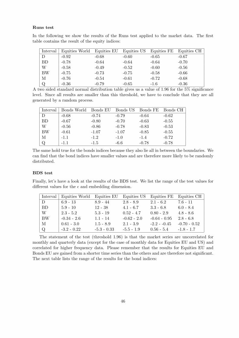
Runs test

In the following we show the results of the Runs test applied to the market data. The firsttable contains the result of the equity indices:

Interval Equities World Equities EU Equities US Equities FE Equities CHD -0.92 -0.68 -0.60 -0.65 -0.67BD -0.78 -0.64 -0.64 -0.64 -0.70W -0.58 -0.49 -0.52 -0.60 -0.56BW -0.75 -0.73 -0.75 -0.58 -0.66M -0.76 -0.54 -0.61 -0.72 -0.68Q -0.36 -0.79 -0.65 -1.6 -0.36

A two sided standard normal distribution table gives us a value of 1.96 for the 5% significancelevel. Since all results are smaller than this threshold, we have to conclude that they are allgenerated by a random process.

Interval Bonds World Bonds EU Bonds US Bonds FE Bonds CHD -0.68 -0.74 -0.79 -0.64 -0.62BD -0.67 -0.80 -0.70 -0.63 -0.55W -0.56 -0.86 -0.78 -0.83 -0.53BW -0.61 -1.07 -1.07 -0.85 -0.55M -1.1 -1.2 -1.0 -1.4 -0.72Q -1.1 -1.5 -6.6 -0.78 -0.78

The same hold true for the bonds indices because they also lie all in between the boundaries. Wecan find that the bond indices have smaller values and are therefore more likely to be randomlydistributed.

BDS test

Finally, let’s have a look at the results of the BDS test. We list the range of the test values fordifferent values for the ε and embedding dimension.

Interval Equities World Equities EU Equities US Equities FE Equities CHD 6.9 - 13 8.9 - 44 2.8 - 8.9 2.1 - 6.2 7.6 - 11BD 5.9 - 10 12 - 38 4.1 - 6.7 3.3 - 6.8 6.0 - 8.4W 2.3 - 5.2 5.3 - 19 0.52 - 4.7 0.80 - 2.9 4.8 - 8.6BW -0.34 - 2.6 1.1 - 14 -0.62 - 2.0 -0.64 - 0.95 2.8 - 6.8M 0.61 - 3.0 1.5 - 8.9 2.1 - 3.9 -2.2 - -0.45 -0.70 - 0.52Q -3.2 - 0.22 -5.3 - 0.33 -5.5 - 1.9 0.56 - 5.4 -1.8 - 1.7

The statement of the test (threshold 1.96) is that the market series are uncorrelated formonthly and quarterly data (except for the case of monthly data for Equities EU and US) andcorrelated for higher frequency data. Please remember that the results for Equities EU andBonds EU are gained from a shorter time series than the others and are therefore not significant.The next table lists the range of the results for the bond indices:

46

Interval Bonds World Bonds EU Bonds US Bonds FE Bonds CHD 1.8 - 4.0 2.7 - 29 3.6 - 5.5 8.9 - 14 -0.27 - 1.44BD 3.3 - 5.5 1.1 - 17 1.4 - 3.1 5.8 - 11 -1.1 - -0.51W 2.1 - 3.8 0.021 - 5.7 2.8 - 3.7 3.7 - 10 -1.2 - 0.12BW 0.26 - 2.6 -1.6 - 3.1 0.056 - 2.2 2.2 - 9.7 -1 - 1.0M -0.89 - 0.76 0.028 - 6.4 -2.6 - 0.23 0.61 - 6.1 -1.4 - 0.88Q -4.2 - 2.0 -1.2 - 8.3 -1.6 - 4.9 0.78 - 3.3 -3.7 - -1.3

We have more or less an acceptance of the hypothesis of uncorrelated returns for bi-weekly,monthly and quarterly data (except for bi-weekly Bonds Far East).

Summary of test results

Let’s summarize the results of the applied tests:

• The Kolmogorov-Smirnov test has shown that the market time series are not normallydistributed, neither on short time frequency (daily data), nor on long time frequency(quarterly data).

• The Jarque-Bera test confirms these statement by refusing normality except for quarterlydata.

• The QQ plots for different sampling frequencies of the data show significant fat tails fordaily up to bi-weekly data

• From the Runs test we were able to conclude that the market series were produced by arandom process

• Finally, the BDS test showed us that the series are uncorrelated for monthly and quarterlydata and correlated for higher frequency data

These results should be evidence enough that the normality assumption of Markowitz doesnot hold and it is justified to look out for other approaches that take non-normality into con-sideration. It was even proposed by Markowitz himself in his Nobel price winning work, alsoto investigate alternatives to variance as risk measures. There are some arguments for thestandard Markowitz method which we don’t want to hide:The Central Limit Theorem says: Let X1, X2, . . . , Xn be mutually independent random vari-ables with a common distribution function F. Assume E[X]= 0 and Var(X)= 1. As n →∞ thedistribution of the normalized sum

Sn =(X1 + X2 + . . . + Xn)√

n

tends to the Gaussian distribution function. When we look at the tick-by-tick logarithmic re-turn data of a stock exchange for a certain financial instrument, we can interpret each datapoint as the value of a random variable and the daily, weekly or monthly data of this instru-ment as the sum of the tick-by-tick returns or the respective random variables. According tothe Central Limit Theorem, the low frequency data will distribute like a Gaussian distributionfunction, if the frequency is low enough and we have enough data points in a period. In thecontext of an index or fund, the Central Limit Theorem can be applied once more by arguingthat an index or fund is the weighted sum of several random variable (the constituents of theindex or fund) and therefore the returns will behave according to a normal distribution if theindex or fund has enough constituents.

47

4 Portfolio Construction With Non Normal Asset Returns

The concept of a mean risk framework was explained an earlier chapter. Markowitz uses thisframework and has the variance chosen as risk measure. We will explore what general propertiessuch a risk measure should have in order to be an substitute for the variance. In the secondpart of this chapter the suitability of variance as risk measure gets analyzed.

4.1 Introduction To Risk In General

In this section we will concentrate on the properties of financial risk measures. Part of the basictheory for this area was developed for the insurance sector and then adapted for the financialcontext.

We will use a variable X as a random variable representing the relative or absolute returnof an asset (or the insured losses in the insurance context). Assume we have two alternativesA and B and their financial consequences XA and XB. Let the function R denote a risk mea-sure which assigns a value to each alternative and the notation A �R B ⇔ R(XA) > R(XB)indicates that the alternative A is riskier then alternative B. Note that this is different fromthe utility function U presented in chapter 1 where A � B ⇔ U(XA) > U(XB) means that Ais preferred to B.The difference of the concepts of the utility function and risk might become more apparent ifone becomes aware that a utility function can be defined without a risk term (e.g. ’prefer moreto less’) or can include a risk term (e.g. Markowitz approach where we can find a trade-offfunction between expected return and risk).

In Albrecht [4] risk measures are categorized into two kinds. The two categories are:1.) Risk as magnitude of deviation from target (risk of the first kind)2.) Risk as necessary capital respectively necessary premium (risk of the second kind)For many common risk measures one kind can get transformed into the other: The addition ofE[X] to a risk measure of the second kind will guide us to a risk measure of the first kind andthe subtraction of E[X] from a risk measure of the first kind will lead to a risk measure of thesecond kind.

We can find a general approach to derive a risk measure for a given utility function. Thisstandard measure of risk is given in Huerlimann [26] by:

R(X) = −E[U(X − E[X])] (21)

Since the risk measure corresponds to the negative expected utility function of X - E[X], therisk measure is location free. From (21) we can derive specific risk measures by using a specificutility function. Using for instance the quadratic utility function (6), we obtain the variance

V ar(X) = E[(X − E[X])2]

as the corresponding risk measure.

We will now introduce the definitions for stochastic and monotonic dominance because theyare useful in the context of risk measures. Assume we are given two random variables X, Y.

48

Stochastic dominance of order 1 for a monotonic function R:

X ≺SD(1) Y ↔ E[R(X)] ≤ E[R(Y )]

Stochastic dominance of order 2 for a concave, monotonic function R:

X ≺SD(2) Y ↔ E[R(X)] ≤ E[R(Y )]

Monotonic dominance of order 2 for a concave function R:

X ≺MD(1) Y ↔ E[R(X)] ≤ E[R(Y )]

Next we will now check some axiomatic systems for risk measures that were proposed in thelast years.

Axiomatic system of Pedersen and Satchell

Pedersen and Satchell give in [32] the following set of axioms for a risk measure:1.) Nonnegativity: R(X) ≥ 0

This requirement follows from the assumption of a risk measure of the first kind (deviationfrom a location measure)

2.) Positive homogeneity: R(c ∗X) = c ∗R(X),∀ constants cIf an investment gets multiplied, then also the risk gets multiplied.

3.) Subadditivity: R(X + Y ) ≤ R(X) + R(Y )The risk or two combined investments will not be larger than the risk of the individual invest-ments (effect of diversification).

4.) Shift invariance: R(X + c) ≤ R(X),∀ constants cThe measure is invariant to an addition of a constant (location free)

Axioms number 2 and 3 combined lead to the statement that the risk of a constant randomvariable must be zero. Axioms 2 and 4 imply that a risk measure according to these criteriais convex. Since the risk measure is assumed to be location free, this system of axioms willdescribe especially risk measures of the first kind.

Axiomatic system of Artzner, Delbaen, Eber and Heath

Artzner, Delbaen, Eber and Heath [7] have developed another set of axioms. Risk measuresthat fulfill their properties are called coherent. The classification was refined in [13] to introducethe terms convex risk measure. Axioms 1 and 4 are also contained in the set of Pedersen andSatchell [32] in a similar way.They call a mapping a convex risk measure if ∀X, Y ∈ <∞,

1.) Subadditivity: R(X + Y ) ≤ R(X) + R(Y )

2.) Monotonicity: X ≤ Y ⇒ R(X) ≥ R(Y )A higher loss potential (statistical dominance) implies a higher risk.

49

3.) Translation Invariance: R(X + a) = R(X)− a,∀ constant returns aThere is no additional risk for an investment without uncertainty.

A convex risk measure R is called a coherent risk measure if it satisfy the additional property:

4.) Positive homogeneity: R(c ∗X) = c ∗R(X),∀ constant c

This set of risk axioms is well suited for risk measures of the second kind. In fact, every reason-able risk measure must be convex because a risk measure that does not satisfy subadditivitypenalizes diversification and would not assign risk in an intuitive way.

Axiomatic system of Wang, Young and Panjier

Another important set of risk axioms was introduced by Wang, Young and Panjier [45]. Theyare dealing with premia in an insurance context, which can however easily be transferred tothe financial context. The two main tasks in insurance markets are the calculation of the riskpremia and the risk capital. The closed system of axioms for premia by Wang, Young andPanjier asks for some continuity properties and

1.) Monotonicity: X ≤ Y ⇒ R(Y ) ≤ R(X)

2.) Comonotone additivity: X1, X2 comonotone ⇒ R(X + Y ) = R(X) + R(Y )

Comonotone: ∃ random variable Z and monotone functions f and g with X = f(Z) andY = g(Z)

A general risk measure

Stone [42] reports a general risk measure containing the three parameters c, k and z as:

R(X) = [∫ z

∞(|x− c|)kf(x)dx]

1k

The standard deviation and semi-standard deviation are part of this general risk measure class.This class was extended in [32] to a five parameter model:

R(X) = [∫ z

∞(|x− c|)aw[F (x)]f(x)dx]b

which contains also the variance, the semi-variance and some other risk measures.

4.2 Variance As Risk Measure

Variance was proposed as appropriate measures for risk by Markowitz in his approach (7). Theadvantage of variance as risk dimension is that it is a very convenient and intuitive measure.It is very common in statistics and has for this reason well known properties. However it hasalso some properties that makes it not optimal as risk measure for financial applications.The risk of very rare events are not taken into account very well by variance. We will show withthe tests presented before that the returns of financial assets often have fat tails. This meansthat extreme events (very high returns or very high losses) are more likely than compared to a

50

normal distribution. In practice of portfolio optimization it is crucial to avoid very high lossesbecause a lot of clients just ask for a preservation of their wealth. It is true that the variancepenalizes extreme events by calculating the squared distance to the mean, however we shouldask for something more specific. For this reason a risk measure that does not pay special at-tention for these kind of events is not very qualified.Another unpleasant property of variance is its symmetry. When we talk about risk, we thinkof the risk for a loss. However variance measures also the ”risk” of a gain, which is in factsomething desired for an investor. This gives rise to asymmetrical risk measures which takeonly care for losses.We have already mentioned that it is shown in [39] that variance is only compatible to thethe concept of a utility function under the assumption of normally distributed returns or aquadratic utility function which is a very strong restriction.

51

5 Value At Risk Measures

In this chapter we will present a first alternative risk measure to the standard deviation. It iscalled Value at Risk and belongs to the quantile based risk measures.There are efforts undertaken to introduce regulations to the financial industry to get a bettercontrol for the risk that is taken by its participants and also to help the companies to get abetter overview for the risk they hold. This was also the topic of the Basel Committee onBanking Supervision where, as a conclusion, they recommend Value at Risk as an appropriaterisk measure.

5.1 Value At Risk

We define Value at Risk as:Let α ∈ (0, 1) be a given probability level and w the asset weights of a portfolio. The Value atRisk at level α for the return R is defined as

V aRα(RP ) = sup{x|P [RP < x] ≤ α} = F−1RP

(α) (22)

The function F−1RP

(α) is called the generalized inverse of the cumulative distribution functionFRP

(x) = P [R ≤ x] of RP and gives the α-quantile of RP .V aRα(RP ) can be interpreted as the loss of a Portfolio that will be exceeded in only α*100percent of all cases. Since α is usually chosen between 0.01 and 0.1, the Value at Risk is a lowerboundary for a portfolio return and the return of the portfolio will with a very high probability(0.99 or 0.9 for the example α) not be smaller. It is the aim of portfolio construction to assemblea portfolio with a high Value at Risk in order to shift the return range for the 1 − α area asmuch to the positive side as possible. Sometimes α is chosen as 0.95 or 0.99 and V aR1−α for aloss function is computed. The similarity of these two notations is shown in appendix B. Figure26 shows two areas α and 1− α for the normal distribution.

Return

Pro

babi

lity

−3 −2 −1 0 1 2 3

0.0

0.1

0.2

0.3

0.4

0.5

α 1−α

x

Figure 26: The Value at Risk at level α for the return R is defined as the return x where the probabilityof having a return smaller than x is α.

52

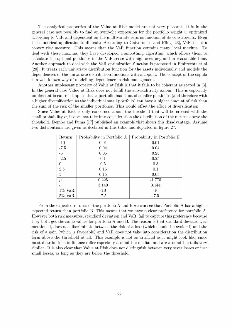
The analytical properties of the Value at Risk model are not very pleasant: It is in thegeneral case not possibly to find an symbolic expression for the portfolio weight w optimizedaccording to VaR and dependent on the multivariate returns function of its constituents. Eventhe numerical application is difficult: According to Gaivoronski and Pflug [23], VaR is not aconvex risk measure. This means that the VaR function contains many local maxima. Todeal with these maxima, they have developed a smoothing algorithm, which allows them tocalculate the optimal portfolios in the VaR sense with high accuracy and in reasonable time.Another approach to deal with the VaR optimization function is proposed in Embrechts et al[20]. It treats each univariate distribution function for the assets individually and models thedependencies of the univariate distribution functions with a copula. The concept of the copulais a well known way of modelling dependence in risk management.

Another unpleasant property of Value at Risk is that it fails to be coherent as stated in [3].In the general case Value at Risk does not fulfill the sub-additivity axiom. This is especiallyunpleasant because it implies that a portfolio made out of smaller portfolios (and therefore witha higher diversification as the individual small portfolio) can have a higher amount of risk thanthe sum of the risk of the smaller portfolios. This would offset the effect of diversification.

Since Value at Risk is only concerned about the threshold that will be crossed with thesmall probability α, it does not take into consideration the distribution of the returns above thethreshold. Dembo and Fuma [17] published an example that shows this disadvantage. Assumetwo distributions are given as declared in this table and depicted in figure 27.

Return Probability in Portfolio A Probability in Portfolio B-10 0.01 0.01-7.5 0.04 0.04-5 0.05 0.25-2.5 0.1 0.250 0.5 0.32.5 0.15 0.15 0.15 0.05µ 0.225 -1.775σ 3.140 3.1441% VaR -10 -105% VaR -7.5 -7.5

From the expected returns of the portfolio A and B we can see that Portfolio A has a higherexpected return than portfolio B. This means that we have a clear preference for portfolio A.However both risk measures, standard deviation and VaR, fail to capture this preference becausethey both get the same values for portfolio A and B. The reason is that standard deviation, asmentioned, does not discriminate between the risk of a loss (which should be avoided) and therisk of a gain (which is favorable) and VaR does not take into consideration the distributionform above the threshold at all. This example is not as artificial as it might look like, sincemost distributions in finance differ especially around the median and are around the tails verysimilar. It is also clear that Value at Risk does not distinguish between very sever losses or justsmall losses, as long as they are below the threshold.

53

Return

Pro

babi

lity

−10 −5 0 5

0.0

0.1

0.2

0.3

0.4

0.5

Figure 27: The graphic shows the two distribution functions defined in the table. The distributionfunction of the returns of portfolio A is depicted as solid line, whereas the distribution function of thereturns of portfolio B is depicted as doted line. The functions are coincident for returns between -10 and-7.5

5.2 Conditional Value At Risk, Expected Shortfall And Tail ConditionalExpectation

In this chapter we will discuss the concepts of Lower Partial Moments (LPM), Conditional Valueat Risk (CVaR) and Expected Shortfall (ES). We cover them in the same chapter because theyare very similar and these risk concepts have become a totum revolutum in the last few years.The following part tries to unveil the relation between the mentioned risk measures.

At the beginning there was a first concept called lower partial moment (LPM) as describedin Fishburn [21]. The general lower partial moment risk measure for a random return variableR and its probability function P (x) is given by

LPMβ(τ ;R) = E[(τ −R)β ] =∫ τ

−∞P (x)(τ − x)βdx

An investor can determine a threshold τ under which he does not want the return R to fall.According to the choice of β, one gets a different lower partial moment:

β = 0 : Shortfall probability LPM0 =∫ τ−∞ f(x)dx

β = 1 : Mean Shortfall LPM1 =∫ τ−∞ f(x)(τ − x)dx

β = 2 : Shortfall variance/ Semi variance LPM2 =∫ τ−∞ f(x)(τ − x)2dx

LPM0 portfolio selection corresponds to Roy’s safety first rule presented in [38]. LPM1,also called expected regret in [16], can be interpreted as the average portfolio underperformancecompared to a fixed target or some benchmark τ .

The term conditional Value at Risk was first introduced in [35]. They use a slightly differentdefinition and notation for VaR and CVaR as we will (refer to appendix B). For continuous dis-tributions conditional Value at Risk is defined as conditional expected loss under the condition

54

that it exceeds the Value at Risk. There are two variants of CVaR:

CV aR+α = E[RP |RP < V aR] (23)

CV aR−α = E[RP |RP ≤ V aR] (24)

where V aR = V aRα(RP ) as defined in formula (22) and E[x] denotes the expected valueof x.As mentioned before, conditional Value at Risk can be considered as expected amount of lossbelow the VaR. From this it gets clear that CV aRα ≤ V aRα

Conditional Value at Risk is also known as Mean Excess Loss (CVaR+), Mean Shortfall(LPM1 with τ = V aR) (CVaR+) or Tail Value at Risk (CVaR−). Since the concept wasdeveloped for several application fields (e.g. actuarial science, finance, economics) and bydifferent researchers, it has many names and definitions. In Huerlimann [25], ten equivalentdefinitions of CVaR are presented. A general definition for CVaR, also applicable for discretedistributions is written in Uryasev [44] as a weighted average of VaR and returns strictly belowVaR. After the conversion to our environment the equation is

CV aRα = λ V aRα + (1− λ) CV aR+α (25)

withλ =

α− P [RP ≤ V aR]α

The equation can be used for continuous and discrete distributions: In the case of a con-tinuous distribution λ = 0 and therefore CV aRα = CV aR+

α . If we have a discrete distributionthe calculated VaR (V aRdisc) will not exactly be the α quantile as it would be for a continuousdistribution (V aRcont), but more on the negative side of the distribution. λ increases CV aR+

α

to the positive side of the distribution and extrapolates CV aR+α from V aRdisc to V aRcont. In

other words, CV aR+α and V aR get weighted proportionally to V aRdisc−V aRcont

V aRcontand therefore

CV aR+α ≤ CV aRα ≤ V aRα.

A similar concept to CVaR is called expected shortfall. It was introduced in [1] and redefinedlater to be consistent with CVaR.

ESα(RP ) = − 1α

(E[RP 1RP≤V aR]− (P [RP ≤ V aR]− α)V aR) (26)

They show in Acerbi and Tasche [2] that it can also be expressed as

ESα(RP ) = − 1α

∫ α

0inf [x|P [X ≤ x] ≥ a]da

In case that we have a non continuous distribution function, it might be that P [RP ≤ x] > α.In contrast, for a continuous distribution function P [RP ≤ x] = α and then it can be seen that(23) is equivalent to (26).

To conclude we try to group the risk measures that have the same base concept. They alltake the distribution function as input and process a number as representant for the risk thedistribution function holds out of the distribution function.

55

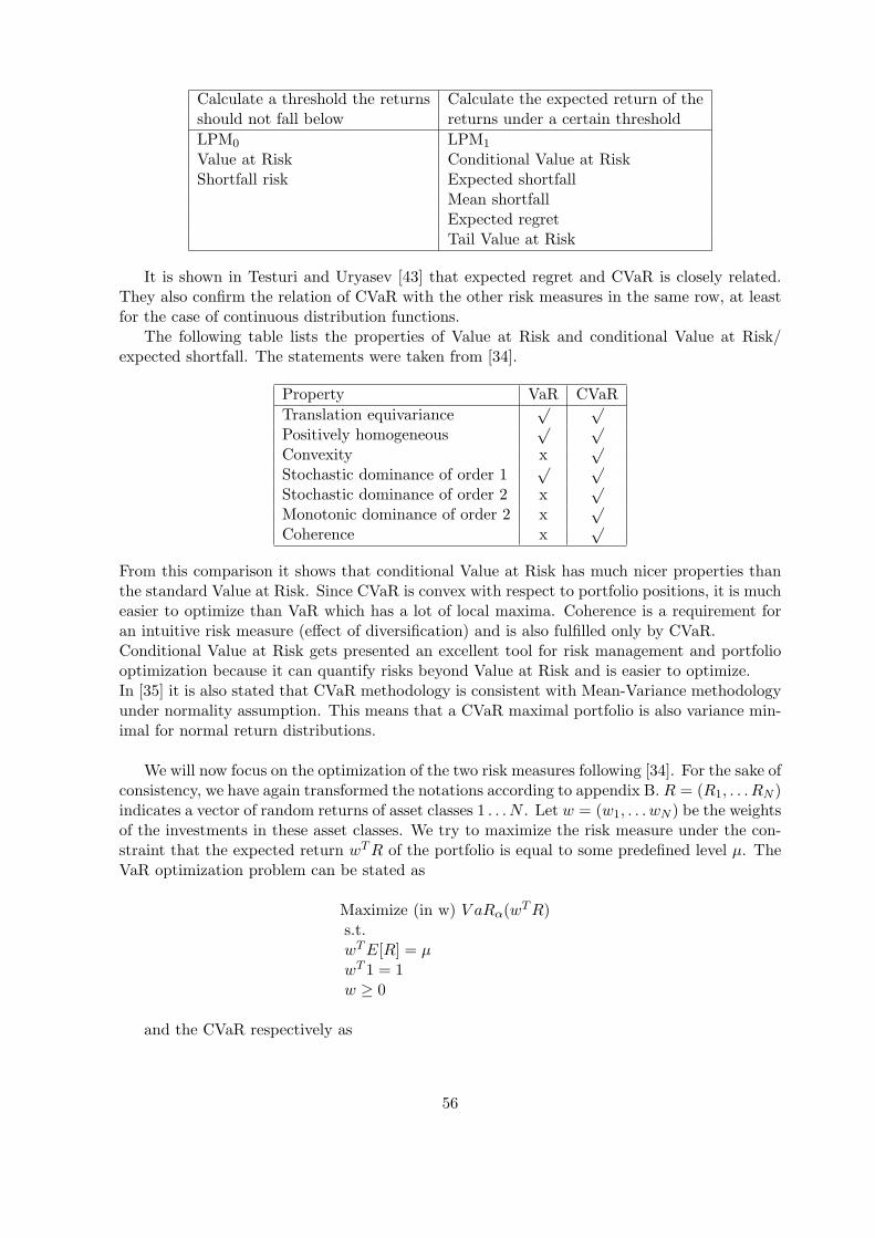
Calculate a threshold the returns Calculate the expected return of theshould not fall below returns under a certain thresholdLPM0 LPM1

Value at Risk Conditional Value at RiskShortfall risk Expected shortfall

Mean shortfallExpected regretTail Value at Risk

It is shown in Testuri and Uryasev [43] that expected regret and CVaR is closely related.They also confirm the relation of CVaR with the other risk measures in the same row, at leastfor the case of continuous distribution functions.

The following table lists the properties of Value at Risk and conditional Value at Risk/expected shortfall. The statements were taken from [34].

Property VaR CVaRTranslation equivariance

√ √

Positively homogeneous√ √

Convexity x√

Stochastic dominance of order 1√ √

Stochastic dominance of order 2 x√

Monotonic dominance of order 2 x√

Coherence x√

From this comparison it shows that conditional Value at Risk has much nicer properties thanthe standard Value at Risk. Since CVaR is convex with respect to portfolio positions, it is mucheasier to optimize than VaR which has a lot of local maxima. Coherence is a requirement foran intuitive risk measure (effect of diversification) and is also fulfilled only by CVaR.Conditional Value at Risk gets presented an excellent tool for risk management and portfoliooptimization because it can quantify risks beyond Value at Risk and is easier to optimize.In [35] it is also stated that CVaR methodology is consistent with Mean-Variance methodologyunder normality assumption. This means that a CVaR maximal portfolio is also variance min-imal for normal return distributions.

We will now focus on the optimization of the two risk measures following [34]. For the sake ofconsistency, we have again transformed the notations according to appendix B. R = (R1, . . . RN )indicates a vector of random returns of asset classes 1 . . . N . Let w = (w1, . . . wN ) be the weightsof the investments in these asset classes. We try to maximize the risk measure under the con-straint that the expected return wT R of the portfolio is equal to some predefined level µ. TheVaR optimization problem can be stated as

Maximize (in w) V aRα(wT R)s.t.wT E[R] = µwT 1 = 1w ≥ 0

and the CVaR respectively as

56

Maximize (in w) CV aRα(wT R)s.t.wT E[R] = µwT 1 = 1w ≥ 0

Note that, since our optimizer is only capable of minimizing a function but not of maximizinga function, we minimize in the implementation −V aRα(wT R) and −CV aRα(wT R).The VaR optimization problem we will cover later. First, we transform the CVaR optimizationproblem in the following linear program with a dummy variable Z:

Maximize (in w and a) a + 1αE[Z]

s.t.Z ≥ wT R− axT E[R] = µwT 1 = 1Z ≥ 0w ≥ 0

Since we have only linear constraints, we can be sure that the solution will be a singleton, aconvex polyhedron or the solution does not exist.In practice however we have mostly discrete variables (e.g. empirical data). For this reason weformulate the portfolio optimization problems in a discrete way.A vector Ri, i = 1, . . . ,M indicates the returns of all asset classes for a certain time point 1,. . .,M. For the formulation we will use a notation S[1:k](u1, . . . , uM ) to denote the one elementamong u1, . . . , uM which is the k-th smallest. The new definitions for VaR and CVaR are

V aRα(wT R) = S[1:bαMc](wT R1, . . . , wT RM )

CV aRα(wT R) =1M

∑wT Ri≤V aRα

wT Ri

The discrete portfolio optimization problem for the VaR is a nonlinear, nonconvex program:

Maximize (in w) S[1:bαMc](wT R1, . . . , wT RM )s.t.wT e = µwT 1 = 1w ≥ 0

where e = 1M

∑Mi=1 Ri denotes the expected return vector.

The discrete version of the CVaR is piecewise linear and may therefore be solved using anLP-solver. We formulate the problem like:

Maximize (in w, a, and z) a + 1αM

∑Mi=1 zi

s.t.zi ≥ −wT Ri − awT e = µwT 1 = 1

57

zi ≥ 0wi ≥ 0

For this setting, the optimal value for a is V aRα(wT R). We can see that the objective functionand the first and third inequality constraint express the weighted average of the Value at Riskand the mean of all negative returns above the Value at Risk (which is the same as the meanof all returns below the negative Value at Risk).

5.3 Mean-Conditional Value At Risk Efficient Portfolios

In this section we want to analyze what it means to optimize a portfolio regarding Value AtRisk/ Conditional Value At Risk.We start with the case of normal distributed asset returns. Figure 28 shows two normal distri-bution with the same mean but different variances. The distribution with the larger variance(doted line) has smaller CVaR and vice-versa. It is intuitive to see that if we maximize theCVaR we also minimize the variance of the distribution. The only way to enlarge the CVaR(shifting the corresponding left tail of the distribution to the right) is to shorten the variance(make the peak larger). Of course this is only true if we a sufficient amount of data comingfrom a pure normal distribution function. Using small amounts of empirical data, there mightbe effects that prevent the equivalence of the two optimization techniques.

−10 −5 0 5 10

0.00

0.05

0.10

0.15

0.20

Return

Pro

babi

lity

CVaRVtlg 1

CVaRVtlg 2

σVtlg 1

σVtlg 2

Figure 28: The graphic shows two normal distribution functions. For both distribution functions theConditional Value at Risk and the variance is schematically depicted. It shows that minimizing thevariance of a function is equivalent to maximizing its Conditional Value at Risk.

58

The case of distributions with skewness and excess kurtosis is more interesting. The oc-currence of fat tails and asymmetry in the distribution function allows the mean-CVaR opti-mization to take the risk evolving out of these properties into account. As consequence, suchan optimization will assign the portfolio weights differently the the Mean-Variance approach.The optimization, in general, will prefer assets with positive skewness, small kurtosis and lowvariance for a given return.

To conclude, we expect the results of a Mean-CVaR and the results of a Mean-Variance op-timization to be the same for the case of similar distribution functions (e.g. normal distributionfunctions) for the asset returns and a sufficient amount of data. Au contraire, the results areassumed to be different for the two optimization techniques if the data is coming from varyingdistribution function with different higher moments or if the sample size is small.

59

6 Draw-Down Measures

In this section we will present two other approaches to measure the risk of a portfolio. They arecalled Draw-Down and Time Under-The-Water. Draw-Down was first presented in a portfoliocontext in [12]. In [33] Draw-Down is used together with Time Under-The-Water to measure theloss potential of hedge funds. We will describe Draw-Down as written in [12] and Time Under-The-Water according the idea in [33]. Afterwards we will enhance Draw-Down to ConditionalDraw-Down at Risk (CDaR) and Time Under-The-Water to Conditional Time Under-The-Water at Risk (CTaR). Finally we apply CDaR in a portfolio context.

6.1 Draw-Down And Time Under-The-Water

An advantage of the two concepts is that they are much more intuitive than other risk mea-sures. The concepts represent values every investor is interested in: Draw-Down measures theloss the investment might suffer (in absolute or relative terms) and Time Under-The-Wateris the time period the investment might remain with a negative performance. Other possibleapplications for these measurements could be: A portfolio manager might loose a client if theclients portfolio does not provide a gain over a long time or a fund might not be allowed toloose more than a certain amount each month and has therefore to stop trading until the nextmonth starts and therefore a new budget.

We will work on the logarithmic returns instead of geometric returns as stated in [12]. Assumewe are given the (cumulated) return of the portfolio from time 0 until time t by a function

rc(w, t)

with w as the vector of weights for the portfolio constituents. The Draw-Down function attime t is defined as the difference between the maximum of the function in the time period [0,t](High-Water-Mark) and the value of the function at time t:

DD(w, t) = max0≤τ≤t[rc(w, τ)]− rc(w, t) (27)

Figure 29 shows a time series with the respective High-Water-Marks and Draw-Down.

Starting with the formula for Draw-Down, two risk functions are derived: Maximum Draw-Down is calculated as the maximum Draw-Down in the period

MD(w, t) = max0≤τ≤t[DD(w, t)] (28)

and the average Draw-Down is defined as

AD(w) =1T

∫ T

0DD(w, t)dt (29)

If, in a time-value framework, Draw-Down is measured on the y-axis, Time Under-The-Wateris the corresponding period on the x-axis that represents the time the value of an investmentmay remain under its historic record mark. We define Time Under-The-Water as

TUW (w, t) = t− [maxT |rc(w,maxT ) = max0≤τ≤trc(w, τ)]

60

0 100 200 300 400 500

−50

050

100

Time

Val

ue

Figure 29: The figure shows a time series with the respective High-Water-Mark (dashed line) and Draw-Down (doted line) as defined. The Time Under-The-Water is just the part of the dashed line above thedoted line.

Similar to the Draw-Down concept, we will now introduce Maximum Time Under-The-WaterMT(w) and Average Time Under-The-Water AT(w) as

MT (w, t) = max0≤τ≤t[TUW (w, t)] (30)

AT (w) =1T

∫ T

0TUW (w, t)dt (31)

6.2 Conditional Draw-Down At Risk And Conditional Time Under-The-Water At Risk

Alike the enhancement of Value at Risk to Conditional Value at Risk, we will proceed withDraw-Down and Time Under-The-Water. Draw-Down at Risk can be defined similar to (22) as

DaRα(MD) = inf{x|P [MD > x] ≤ α} (32)

with MD as Maximum Draw-Down and Conditional Draw-Down at Risk corresponding toConditional Value at Risk (25) as:

CDaRα = λ DaRα + (1− λ) CDaR+α (33)

with

λ =P [MD ≥ DaRalpha]− α

α

CDaR+α = E[MD|MD > DaRα] (34)

61

We will now discuss the implementation of the concepts in detail. A first approach wouldbe to calculate the Maximum Draw-Down for each new level of the High-Water-Mark. Thismeans, we scan the time series from the past to the present and each time we find a new globalmaxima, we calculate the Maximum Draw-Down for the period between this global maximaand the point where the time series is higher than this global maxima for the first time. All ofthese Maximum Draw-Downs get stored to construct their distribution. The drawback of thismethod is that we will probably get very few Draw-Down values for the following reasons:

• Since the Draw-Down gets calculated as the difference to the highest historical value(record), the concept of the Draw-Down comprises the effect of increasing time periodsfor new records: The expected time period for a random variable to reach a new all-time-high is not uniformly distributed but increases much faster over time (see for example[19]).

• In times of a Baise, we won’t get any Draw-Downs at all. Only in times of a Hausse therewill be a new High-Water-Mark and therefore new Draw-Downs.

In [12] it was proposed to introduce M sub-periods in the time interval [0,T] and to calculatethe Draw-Down for each sub-period. This way they get an empirical distribution for the Draw-Downs consisting out of maximum M sample points. Using this methodology, one should beaware of some points:

• The methodology adds a new variable M that does not improve the descriptive power ofthe concept. The reason for introducing this variable is just for numerical reasons andhas no economical or practical meaning.

• If M is chosen too large, the number of resulting Draw-Downs is too small to get agood distribution approximation. If M is chosen too small, the Draw-Downs that extendover several sub-periods get cut into several smaller Draw-Downs because the maximumpossible Draw-Down is restricted to the length of the sub-period. This is especiallyundesirable since we are particularly interested in the large Draw-Downs to calculate theα-quantile.

• The effect of increasing time periods for new records can not be avoided by resetting theall-time-high at the beginning of each sub-period - it is just transformed to a smaller timescale.

We would like to bring this method and a new method into the context of the informationgiven by the client. The described method of the fixed periods for calculating the Draw-Downcould be used if the investment horizon of the client is known:

If the investment horizon is known, a rolling window with the length of the investment hori-zon could be applied to the available historical data. For each time window the MaximumDraw-Down gets calculated and the window shifted for one period. If we have P historical datapoints, Q data points in the rolling window and shift the window R data points each time weadvance, we get with this method P−Q

R Maximum Draw-Down values. It would also be possibleto use overlapping rolling windows. However this would decrease the variance of the in thisway reused data.

If the investment horizon is not known, we propose as a second method to calculate the Max-imum Draw-Down for each possible entry combined with each possible exit point. This gives

62

us for P data points (P−1)(P−2)2 Maximum Draw-Down values. The idea is to calculate the

average Draw-Down an investor could face. The disadvantage of this method is that the Draw-Down values for a certain (unknown) investment horizon have very few influence to the finaldistribution. The reason for this is that the number of possible Draw-Downs grows quadratical,however the number of Draw-Downs for a certain investment period grows only linearly. Itmight therefore be questionable to compare Draw-Downs of different time periods.

We will assume that the investment horizon is known and therefore proceed with the first ofthe described methods to formulate the optimization problems.

It lies in the nature of the concept to change the structure of the optimization problem from”minimize the risk for a given expected return”, as it was the case for Variance and CVaR op-timization, to ”maximize the expected return for a given Draw-Down/Time Under-The-Waterthreshold”. For an investor it is convenient to define his/her personal amount of wealth he/sheis willing to risk or the amount of time he/she gives to the portfolio manager to remain witha negative performance. However, to be better able to compare the results of the differentoptimizations, we will stick to our old schema of fixing an expected return and minimizing therespective risk measure.

To show the corresponding linear optimization problems, we introduce the following vari-ables: The vector of logarithmic cumulative asset returns up to time moment k be yk so we cancalculate the cumulative portfolio return as rc(w, t = k) = yk ∗ w. With the expected returngiven by the investor as µ, we get the following linear programming problem for the MaximumDraw-Dawn

Minimize (in w and u) zs.t.uk − yk ∗ w ≤ z 1 ≤ k ≤ Muk ≥ yk ∗ w, 1 ≤ k ≤ Muk ≥ uk−1, 1 ≤ k ≤ Mu0 = 01dyM ∗ w = µ

wT 1 = 1wi ≥ 0, 1 ≤ i ≤ N

where uk , 1 ≤ k ≤ M and z are auxiliary variables and d is the investment period in years.

The optimization problem with a constraint on the average Draw-Down can be written asfollows

Minimize (in w and u) zs.t.1M

∑Mk=1(uk − yk ∗ x) ≤ z

uk ≥ yk ∗ x, 1 ≤ k ≤ Muk ≥ uk−1, 1 ≤ k ≤ Mu0 = 01dyM ∗ x

wT 1 = 1wi ≥ 0, 1 ≤ i ≤ N

63

and the optimization problem with a constraint on CDaR may be formulated as

Minimize (in w, u, z, ζ) zs.t.ζ + 1

αM

∑Mk=1 zk ≤ z

zk ≥ uk − yk ∗ x− ζ, 1 ≤ k ≤ Mzk ≥ 0, 1 ≤ k ≤ Muk ≥ yk ∗ x, 1 ≤ k ≤ Muk ≥ uk−1, 1 ≤ k ≤ Mu0 = 01dyT ∗ xwT 1 = 1wi ≥ 0, 1 ≤ i ≤ N

The optimal solution of this problem gives the optimal threshold value in variable ζ.

The corresponding extension of the Time Under-The-Water to a risk measure ConditionalTime Under-The-Water at Risk (CTaR) can be done similarly.

Since the optimization problems are analogous to the ones of Draw-Down, we will give only thelinear programm for the Conditional Time Under-The-Water at Risk

Minimize (in w, u, z, ζ) vs.t.ϑ + 1

αM

∑Mk=1 zk ≤ v

zk ≥ uk − yk ∗ x− ϑ, 1 ≤ k ≤ Mzk ≥ 0, 1 ≤ k ≤ Muk ≥ yk ∗ x, 1 ≤ k ≤ Muk ≥ uk−1, 1 ≤ k ≤ M1dyT ∗ xu0 = 0wM1 = 1wi ≥ 0, 1 ≤ i ≤ N

where uk , zk, 1 ≤ k ≤ M and v are auxiliary variables.

A well implementable setup for the portfolio optimization process (that we will not furtherfollow) would be the following framework: Optimize the expected portfolio return subject tothe clients CDaR restriction ζC and CTaR restriction ηC .

Maximize 1dC yM ∗ x

s.t.CDaRα(w) ≤ ζC

CTaRα(w) ≤ ηC

64

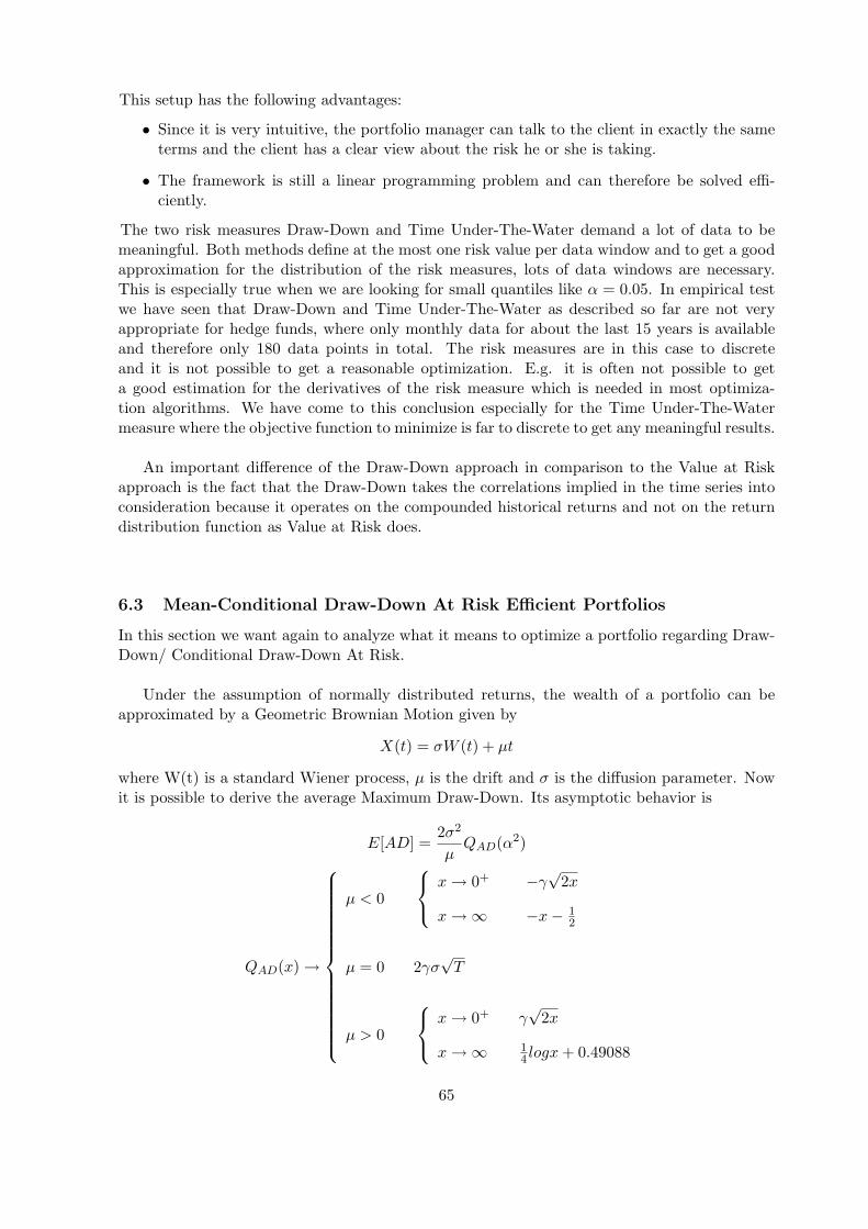
This setup has the following advantages:

• Since it is very intuitive, the portfolio manager can talk to the client in exactly the sameterms and the client has a clear view about the risk he or she is taking.

• The framework is still a linear programming problem and can therefore be solved effi-ciently.

The two risk measures Draw-Down and Time Under-The-Water demand a lot of data to bemeaningful. Both methods define at the most one risk value per data window and to get a goodapproximation for the distribution of the risk measures, lots of data windows are necessary.This is especially true when we are looking for small quantiles like α = 0.05. In empirical testwe have seen that Draw-Down and Time Under-The-Water as described so far are not veryappropriate for hedge funds, where only monthly data for about the last 15 years is availableand therefore only 180 data points in total. The risk measures are in this case to discreteand it is not possible to get a reasonable optimization. E.g. it is often not possible to geta good estimation for the derivatives of the risk measure which is needed in most optimiza-tion algorithms. We have come to this conclusion especially for the Time Under-The-Watermeasure where the objective function to minimize is far to discrete to get any meaningful results.

An important difference of the Draw-Down approach in comparison to the Value at Riskapproach is the fact that the Draw-Down takes the correlations implied in the time series intoconsideration because it operates on the compounded historical returns and not on the returndistribution function as Value at Risk does.

6.3 Mean-Conditional Draw-Down At Risk Efficient Portfolios

In this section we want again to analyze what it means to optimize a portfolio regarding Draw-Down/ Conditional Draw-Down At Risk.

Under the assumption of normally distributed returns, the wealth of a portfolio can beapproximated by a Geometric Brownian Motion given by

X(t) = σW (t) + µt

where W(t) is a standard Wiener process, µ is the drift and σ is the diffusion parameter. Nowit is possible to derive the average Maximum Draw-Down. Its asymptotic behavior is

E[AD] =2σ2

µQAD(α2)

QAD(x) →

µ < 0

x → 0+ −γ√

2x

x →∞ −x− 12

µ = 0 2γσ√

T

µ > 0

x → 0+ γ√

2x

x →∞ 14 logx + 0.49088

65

α = µ√

(T

2σ2)

γ =√

(π

8)

with T as the investment horizon. This setup allows us to estimate the average Draw-Down ofa time series by using its mean and variance. Again, we made the experience that in practisea lot of data is necessary to get a reasonable result. The reason might lie in the assumptionof normality in the returns distribution which can be hold, if ever, only for very long time series.

If normality does not hold, the portfolio or assets wealth can not be modelled by a GeometricBrownian Motion and therefore the algebraic relation is not valid anymore.

66

7 Comparison Of The Risk Measures

Peijan and Lopez de Prado state in [33] that there is also an algebraic relation between VaR,Draw-Down and Time Under-The-Water whenever normality and time-independence hold. Insection 5.3 we have seen that variance is closely related to CVaR and in section 6.3 we haveshown that there exists an algebraic correspondence between variance and Draw-Down for thecase of normality.This means that there is even an algebraic correspondence between Variance, Value at Risk,Draw-Down and Time Under-The-Water. And for the context of portfolio optimization we canconclude that the three optimization techniques minimizing the variance, minimizing CDaRand maximizing CVaR will end up with the same results if the assumptions of normality andtime-independence hold.This relation between the different risk measures disappears when normality can not be assumedanymore and we expect the optimization procedures to produce different results.

67

Part III

Optimization With Alternative Investments

This third part deals with the implementation of the discussed risk measures and the resultsachieved by using different data sets. Therefore we first show the implemented optimizationproblems and some numerical specialities related to them. Then we discuss quickly the differentkind of data and show the used data. Afterwards the results of the calculations are shown andinterpreted. Finally a summary and an outlook is given.

8 Numerical Implementation

The table below summarizes the considered optimization problems whereby µ indicates theexpected return given by the investor.

Min V ariance Max CV aR Min CDaR

E[R] = µ E[R] = µ E[R] = µ∑wi = 1

∑wi = 1

∑wi = 1

wi ≥ 0 wi ≥ 0 wi ≥ 0

In the following we list some aspects of the implementation:

• Since our optimizer is only capable of minimizing a function but not of maximizing afunction, we minimize in the implementation −CV aR instead of maximizing CV aR.

• We do not minimize the Variance but the standard deviation. Experiments have shownthat this results in a better convergence of the solution. The reason might lie in theoptimization algorithm that seeks the lowest value of a function by following the steep-est gradient. Since we are mostly dealing with variances smaller than 1, the standarddeviation - as square root of the variance - has a ”broader minimum”.

• In order to get the best results the efficient frontier gets calculated twice: A first runstarts at the corner solution with the lowest expected return moving to the corner solutionoffering the highest expected return and afterwards a second run is executed in reverseorder. The results of the first run are stored and compared with the results of the secondrun, whereby the better results (i.e. the portfolio weights leading to a smaller risk value)are chosen for the final output. While moving from one corner solution to the other, theoptimal portfolios are calculated. The optimizer can be given an initial estimation forthe weights of the optimal portfolio. These estimations of the optimal portfolio weightsare calculated as linear extrapolation of the last two optimal portfolio weights becauseportfolio weights change often linearly while changing the expected return.

68

9 Used Data

In this section we will explain the difference between normal and logarithmic data and arguewhy we have decided to use logarithmic data. We also list the used historical market data andshow how we have simulated artificial data from it.

9.1 Normal Vs. Logarithmic Data

In finance there are two common ways to model returns: Simple/geometric returns and loga-rithmic/ continuously compounded returns. The following table gives an overview of geometricand logarithmic returns for single- and multi-period each. PtandPt+1 denote the absolute valueof the asset at time point t and t+1 respectively.

Single-period Multi-period

Geometric Return Rt,t+1 = Pt+1

Pt− 1 Rt,t+n = [

∏n−1i=0 (1 + Rt+i,t+i+1)]− 1

Logarithmic Return rt,t+1 = log(1 + Rt,t+n) rt,t+n = log[∏n−1

i=0 (1 + Rt+i,t+i+1)]=

∑n−1i=0 rt+i,t+i+1

With geometric returns, the new return gets calculated at the end of each period andtherefore the increase or decrease in the return gets active for the next period. In contrast, usingcontinuously compounded returns, the change in the returns gets calculated on a infinitesimalsmall time period and therefore a continuously compounded return represents the actual valueat every time point.

We have decided to use logarithmic/continuously compounded returns for the analysis forthe following reasons:

• Because 0 ≥ Pt+n

Pt≥ ∞, using simple returns, the effective return can not be below -1

(full loss, for Pt+n = 0) which is an restriction to the range of possible values. Usinglogarithmic returns, the range gets stretched to [−∞,∞]. This is especially importantfor tail analysis, since the tail gets cut at -1 using simple returns and there would be aprobability assigned to value that do not appear.

• If single-period returns are assumed to be normal, then multi-period returns (∏

i(1 +Rt+i)) − 1 are not normal. This comes from that the fact that a product of normallydistributed variables is not normally distributed. By taking log-returns, multi-periodreturns are achieved by adding up the single-period returns which results again in anormal distribution (Central Limit Theorem)

• The concepts of CVaR, CDaR calculate thresholds that may lie in between a time periodwhereas the data is for the end of the time period. In this case it is more precise to uselogarithmic returns instead of the linear approximation done by geometric returns.

69

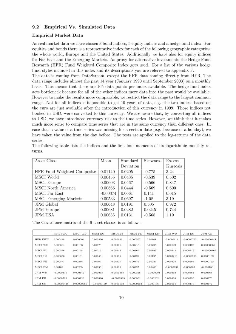
9.2 Empirical Vs. Simulated Data

Empirical Market Data

As real market data we have chosen 3 bond indices, 5 equity indices and a hedge fund index. Forequities and bonds there is a representative index for each of the following geographic categories:the whole world, Europe and the United States. Additionally we have also for equity indicesfor Far East and the Emerging Markets. As proxy for alternative investments the Hedge FundResearch (HFR) Fund Weighted Composite Index gets used. For a list of the various hedgefund styles included in this index and its descriptions you are referred to appendix F.The data is coming from DataStream, except the HFR data coming directly from HFR. Thedata range includes almost the past 14 year (January 1990 until September 2003) on a monthlybasis. This means that there are 165 data points per index available. The hedge fund indexacts bottleneck because for all of the other indices more data into the past would be available.However to make the results more comparable, we restrict the data range to the largest commonrange. Not for all indices is it possible to get 10 years of data, e.g. the two indices based onthe euro are just available after the introduction of this currency in 1999. Those indices notbooked in USD, were converted to this currency. We are aware that, by converting all indicesto USD, we have introduced currency risk to the time series. However, we think that it makesmuch more sense to compare time series that are in the same currency than different ones. Incase that a value of a time series was missing for a certain date (e.g. because of a holiday), wehave taken the value from the day before. The tests are applied to the log-returns of the dataseries.The following table lists the indices and the first four moments of its logarithmic monthly re-turns.

Asset Class Mean Standard Skewness ExcessDeviation Kurtosis

HFR Fund Weighted Composite 0.01140 0.0205 -0.775 3.24MSCI World 0.00455 0.0435 -0.539 0.502MSCI Europe 0.00603 0.0467 -0.566 0.847MSCI North America 0.00866 0.0444 -0.569 0.600MSCI Far East -0.00374 0.0661 0.141 0.615MSCI Emerging Markets 0.00533 0.0697 -1.08 3.19JPM Global 0.00648 0.0191 0.505 0.972JPM Europe 0.00681 0.0282 0.0245 0.744JPM USA 0.00635 0.0131 -0.568 1.19

The Covariance matrix of the 9 asset classes is as follows:

HFR FWC MSCI WD MSCI EU MSCI US MSCI FE MSCI EM JPM WD JPM EU JPM US

HFR FWC 0.000418 0.000604 0.000576 0.000636 0.000577 0.00108 -0.0000111 -0.0000705 -0.00000448

MSCI WD 0.000604 0.00188 0.00178 0.00161 0.00218 0.00205 0.000149 0.000120 0.00000066

MSCI EU 0.000576 0.00178 0.00216 0.00143 0.00167 0.00193 0.000213 0.000316 -0.00000169

MSCI US 0.000636 0.00161 0.00143 0.00196 0.00121 0.00195 0.0000218 -0.0000999 0.0000102

MSCI FE 0.000577 0.00218 0.00167 0.00121 0.00435 0.00227 0.000328 0.000301 0.0000152

MSCI EM 0.00108 0.00205 0.00193 0.00195 0.00227 0.00483 -0.0000991 -0.000262 -0.000156

JPM WD -0.0000111 0.000149 0.000213 0.0000218 0.000328 -0.0000991 0.000362 0.000468 0.000164

JPM EU -0.0000705 0.000120 0.000316 -0.0000999 0.000301 -0.000262 0.000468 0.000790 0.000170

JPM US -0.00000448 0.00000066 -0.00000169 0.0000102 0.0000152 -0.000156 0.000164 0.000170 0.000172

70

Simulated data

We generate artificial data based on the historical data described above. For this purpose we firstfit a multivariate skewed normal distribution and a multivariate skewed student-t distributionto the historical data. The fitting procedure gives us a vector of regression coefficients, thecovariance matrix, a vector of shape parameters and the degree of freedom. In the case offitting a skewed normal distribution the shape parameters are all 0 and the degree of freedomis infinite as it is well-know for the normal distribution.Based on this estimated distributions we can generate random samples. As always with MonteCarlo Simulations, we have the advantage that we have full control over the underlying modelbecause we can control and change the parameters. As disadvantage we note that the MonteCarlo ignores all dependencies over time in the time series and therefore slightly overstate thetrue value of diversification across assets classes in simulated portfolios.Another unpleasant aspect is that there is only one value for the degree of freedom for all assetclasses estimated and respected in the fitted function. This means that the time series do nothave an individual kurtosis each but only a common one. However it is a non-trivial task togenerate multivariate correlated data with skewness and kurtosis and would be beyond thescope of this thesis. One approach would be to use Copulas.

71

10 Evaluation Of The Portfolios

So far we have presented three methods how it could be possible to optimize a portfolio and inthe last chapter we have introduced some historical market data. In the following part we willpublish the portfolios that were optimized based on the market data. In a first section we showthe results of the portfolio optimization if we use only traditional assets classes. Afterwards weintroduce a hedge fund and analyze how it changes the optimal portfolios. In the third partwe generate artificial data with the same characteristics as the asset classes and optimize thisdata.For the portfolio optimization we give the expected return of the investor and try to minimizethe respective risk. This procedure is done for several expected returns to get the efficient fron-tier. For the calculations, the range of these expected returns is defined as the interval betweenthe smallest and the largest expected return of the assets classes. Clearly, under the assumptionof no short sales and no lending and borrowing it is not possible to reach an expected portfolioreturn outside this interval (see chapter 1.2). We are aware that the part of the efficient frontierthat is below the minimum risk portfolio is in practise not relevant. This is especially true forexpected target returns below 0. We will nevertheless show the whole range to give the wholepicture of the optimization results and to compare them.For the charts we use the following color encoding:

Asset Class Color Style ExampleHFR Fund Weighted Composite Black SolidMSCI World Orange SolidMSCI Europe Red SolidMSCI North America Green SolidMSCI Far East Blue SolidMSCI Emerging Markets Pink SolidJPM Global Orange DashedJPM Europe Red DashedJPM USA Green Dashed

The alpha value for the CVaR and CDaR optimization is chosen as 0.25, the size of therolling window for the CDaR as 24 and the step size for the CDaR as 3. These are the values forwhich we got the most stable results. Since we have only 165 data points per time series, it wasnot possible to decrease the alpha value further towards 0.1 or use non-overlapping windowsfor the calculation of CDaR and still get reasonable results.For the portfolio optimization no constraints for the weights were introduced in order to seethe pure results and no influenced ones.

10.1 Evaluation With Historical Data

This section contains the results derived by using the original data series as presented before.All the calculations are done for the 8 traditional asset classes and again for the 9 asset classesincluding the hedge fund data.

72

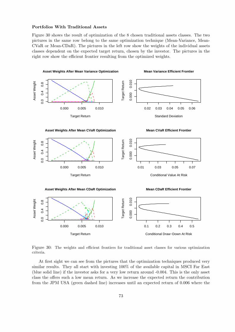
Portfolios With Traditional Assets

Figure 30 shows the result of optimization of the 8 chosen traditional assets classes. The twopictures in the same row belong to the same optimization technique (Mean-Variance, Mean-CVaR or Mean-CDaR). The pictures in the left row show the weights of the individual assetsclasses dependent on the expected target return, chosen by the investor. The pictures in theright row show the efficient frontier resulting from the optimized weights.

0.000 0.005 0.010

0.0

0.4

0.8

Target Return

Ass

et W

eigh

t

Asset Weights After Mean Variance Optimization

0.02 0.03 0.04 0.05 0.06

0.00

00.

010

Standard Deviation

Tar

get R

etur

n

Mean Variance Efficient Frontier

0.000 0.005 0.010

0.0

0.4

0.8

Target Return

Ass

et W

eigh

t

Asset Weights After Mean CVaR Optimization

0.01 0.03 0.05 0.07

0.00

00.

010

Conditional Value At Risk

Tar

get R

etur

n

Mean CVaR Efficient Frontier

0.000 0.005 0.010

0.0

0.4

0.8

Target Return

Ass

et W

eigh

t

Asset Weights After Mean CDaR Optimization

0.1 0.2 0.3 0.4 0.5

0.00

00.

010

Conditional Draw−Down At Risk

Tar

get R

etur

n

Mean CDaR Efficient Frontier

Figure 30: The weights and efficient frontiers for traditional asset classes for various optimizationcriteria.

At first sight we can see from the pictures that the optimization techniques produced verysimilar results. They all start with investing 100% of the available capital in MSCI Far East(blue solid line) if the investor asks for a very low return around -0.004. This is the only assetclass the offers such a low mean return. As we increase the expected return the contributionfrom the JPM USA (green dashed line) increases until an expected return of 0.006 where the

73

contribution of MSCI Far East is decreased to a contribution of 0. In this area we can seedifferences in the asset allocation of the three techniques: The Mean Variance optimizationpushes the JPM USA class to 100% to reach an expected return of 0.006, whereas Mean CDaRincreases JPM USA to 0.8 at the maximum and distributes the resulting part to JPM global(turquoise doted line). All three techniques agree in the range above 0.007 to invest in JPMEurope (red doted line) and have a major allocation in MSCI North America when it comes toan expected return above 0.008.The efficient frontier also look very similar for all three optimization techniques. The minimumrisk portfolio is at an expected return of 0.0065 for all techniques. We can state that the efficientfrontier of Mean Variance and Mean CVaR are more similar in comparison with the efficientfrontier of Mean CDaR optimization.The results do not correspond completely to the portfolio theory which says that in the areaof lower expected return we can find mostly bonds because they offer usually a lower expectedreturn and a low risk. In the higher region of expected returns we could expect equity indicesfrom risky geographic locations as the Emerging Markets.We can explain the calculated results with the actual situation at the world markets: Thetable with the four moments of the indices show that MSCI Far East is the only index with anegative first moment. The reason for this is the Asia crisis in 1997 that is contained in thedata interval. The second moment shows us why indices like MSCI Emerging Markets andMSCI Europe don’t appear in the weights chart: They have a too high Standard Deviation -especially in comparison to the bonds which offer a higher expected return for a lower StandardDeviation. Since the three optimizations are linked together via the standard deviation, thisholds true for all of them.The results also show the effect of diversification very clearly: MSCI Far East (blue solid line)and JPM US (green dashed line) which dominate the lower part of expected return have acorrelation of -0.0001 (see Covariance matrix) and MSCI US (green solid line) together withJPM EU (red dashed line), which have a high allocation in the higher part of expected return,have a correlation of -0.0000152. These are two of the smallest entries in the Covariance matrix.This shows that all optimization techniques try to combine the fewest correlated assets.This might also be the reason why MSCI World Equities is used so rarely to form the port-folios: MSCI World can be considered as a linear combination of the other indices. Since theoptimization is looking for optimal diversification, the other indices, that inherit more extremeproperties, are being used.The results of the Mean-Variance optimization are very smooth, whereas the efficient frontier ofthe Mean-CDaR optimization is much more peaked and unstable. This effect might be comingfrom the small data set and the fact that CDaR (and also CVaR to a certain extent) takeoutliers heavily into consideration. As we will see, this artifacts will disappear as soon as weincrease the amount of data.

74

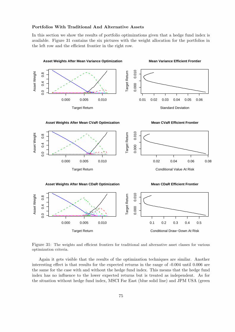
Portfolios With Traditional And Alternative Assets

In this section we show the results of portfolio optimizations given that a hedge fund index isavailable. Figure 31 contains the six pictures with the weight allocation for the portfolios inthe left row and the efficient frontier in the right row.

0.000 0.005 0.010

0.0

0.4

0.8

Target Return

Ass

et W

eigh

t


0.01 0.02 0.03 0.04 0.05 0.06

0.00

00.

010

Standard Deviation

Tar

get R

etur

n


0.000 0.005 0.010

0.0

0.4

0.8

Target Return

Ass

et W

eigh

t


0.02 0.04 0.06 0.08

0.00

00.

010


Tar

get R

etur

nMean CVaR Efficient Frontier

0.000 0.005 0.010

0.0

0.4

0.8

Target Return

Ass

et W

eigh

t


0.1 0.2 0.3 0.4 0.5

0.00

00.

010


Tar

get R

etur

n


Figure 31: The weights and efficient frontiers for traditional and alternative asset classes for variousoptimization criteria.

Again it gets visible that the results of the optimization techniques are similar. Anotherinteresting effect is that results for the expected returns in the range of -0.004 until 0.006 arethe same for the case with and without the hedge fund index. This means that the hedge fundindex has no influence to the lower expected returns but is treated as independent. As forthe situation without hedge fund index, MSCI Far East (blue solid line) and JPM USA (green

75

dashed line) dominate the range between -0.004 and 0.006. Around the expected return of0.005 we have for the Mean CDaR and Mean CVaR optimization also JPM Global (turquoisedashed line) playing a minor role. The hedge fund index gets taken into consideration whenthe expected return reaches a level of 0.006 and above. It attracts all the weight for expectedreturns above 0.010 because it is the only asset offering such a high return. Remarkable is thatJPM Europe (red dashed line) gets over weighted in a Mean CDaR optimization in comparisonto Mean Variance and Mean CVaR optimizations.The Covariance matrix shows that the hedge fund index is very little correlated with the otherassets. The results of the optimization suggest to combine the hedge fund index with JPMEU (red dashed line) and JPM US (green dashed line) to get a high expected portfolio return.The correlation of the hedge fund index is negative with both Bond indices. Again the effectof diversification got utilized by all of the optimization techniques.The little peaks in the weight allocation charts show that the CDaR-results are much moreinstable compared to the Variance-Results.

10.2 Evaluation With Simulated Data

In this section we will optimize portfolios based on simulated data. As earlier described, thedata is gained by fitting a distribution to the available monthly time series of the assets classes.We distinguish between fitting a skewed normal distribution and fitting a skewed student-tdistribution. As soon as we have the distribution, we can generate as many artificial data withthe same properties as we need. For the following calculations we have generated 2000 samplesfor each asset class. This represents 2000 months or 167 years of data.

Portfolios With Simulated Traditional Assets

Figure 32 shows that the results we get when fitting a multivariate skew normal distributionto the historical data and generating 2000 samples with this distribution are pretty muchsimilar to the ones of the original data. We can see that the instability in the CDaR andCVaR optimization disappears and all of the three optimizations get the same results. Onlya little peak of 10 percent allocation in MSCI Emerging Markets in the CDaR optimizationdistinguishes the results.In Figure 33 the results for fitting a multivariate student-t distribution to the same 8 dataseries are provided. The covered range for the expected return has shifted from the interval(-0.004, 0.008) to the interval (-0.001, 0.010) which is a results of the randomly generation ofnew data from the fitted distribution. Besides this shift there is another difference comparedto fitting a skewed normal distribution: The allocation of JPM Europe (dotted red line) ismore varying comparing the three optimization techniques. It fluctuates from 20 percent forMean-Variance optimization up to almost 40 percent for Mean-CDaR optimization. This effectmight be coming from the fitted skewed student-t distribution that allows a higher adaptationto the original data then the skewed normal distribution.

76

0.000 0.005 0.010

0.0

0.4

0.8

Target Return

Ass

et W

eigh

t


0.02 0.03 0.04 0.05 0.06 0.07

0.00

00.

010

Standard Deviation

Tar

get R

etur

n


0.000 0.005 0.010

0.0

0.4

0.8

Target Return

Ass

et W

eigh

t


0.02 0.04 0.06 0.08

0.00

00.

010


Tar

get R

etur


0.000 0.005 0.010

0.0

0.4

0.8

Target Return

Ass

et W

eigh

t


0.1 0.2 0.3 0.4 0.5 0.6

0.00

00.

010


Tar

get R

etur

n


Figure 32: The weights and efficient frontiers for traditional asset classes for various optimizationcriteria. The used data has been simulated by a skewed normal distribution fitted to the historical data.

77

0.000 0.005 0.010

0.0

0.4

0.8

Target Return

Ass

et W

eigh

t


0.01 0.02 0.03 0.04 0.05 0.06

0.00

00.

010

Standard Deviation

Tar

get R

etur

n


0.000 0.005 0.010

0.0

0.4

0.8

Target Return

Ass

et W

eigh

t


0.01 0.02 0.03 0.04 0.05 0.06 0.07

0.00

00.

010


Tar

get R

etur


0.000 0.005 0.010

0.0

0.4

0.8

Target Return

Ass

et W

eigh

t


0.1 0.2 0.3 0.4 0.5

0.00

00.

010


Tar

get R

etur

n


Figure 33: The weights and efficient frontiers for traditional asset classes for various optimizationcriteria. The used data has been simulated by a skewed student-t distribution fitted to the historicaldata.

78

Portfolios With Simulated Traditional Assets And Alternative Assets

Figure 34 and figure 35 show the result for the 9 assets classes, including the hedge fund index.The results of figure 34 are retrieved by fitting a skewed normal distribution to the historicaldata, whereas the results of figure 35 are retrieved by fitting a skewed student-t distribution tothe historical data.

0.000 0.005 0.010

0.0

0.4

0.8

Target Return

Ass

et W

eigh

t


0.01 0.02 0.03 0.04 0.05 0.06

0.00

00.

010

Standard Deviation

Tar

get R

etur

n


0.000 0.005 0.010

0.0

0.4

0.8

Target Return

Ass

et W

eigh

t


0.02 0.04 0.06 0.08

0.00

00.

010


Tar

get R

etur


0.000 0.005 0.010

0.0

0.4

0.8

Target Return

Ass

et W

eigh

t


0.1 0.2 0.3 0.4 0.5 0.6

0.00

00.

010


Tar

get R

etur

n


Figure 34: The weights and efficient frontiers for traditional and alternative asset classes for variousoptimization criteria. The used data has been simulated by a skewed normal distribution fitted to thehistorical data.

Comparing figure 34 and figure 35 we see again the same effect as we have seen for the 8asset classes: the outcome of the three different optimizations differs more when we fit thehistorical data with a multivariate skewed student-t distribution instead of the multivariateskewed normal distribution. Besides this we can confirm that hedge funds offer a possibility forhigher returns.

79

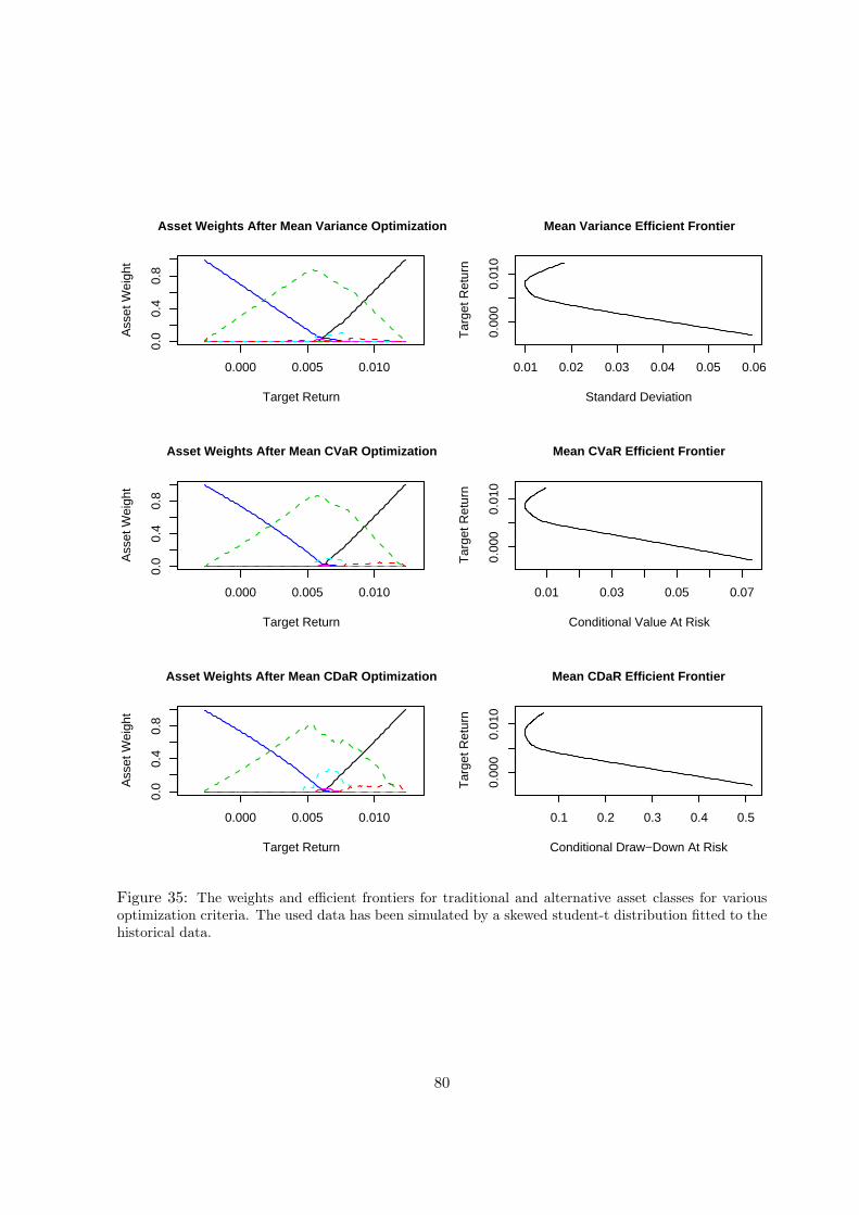
0.000 0.005 0.010

0.0

0.4

0.8

Target Return

Ass

et W

eigh

t


0.01 0.02 0.03 0.04 0.05 0.06

0.00

00.

010

Standard Deviation

Tar

get R

etur

n


0.000 0.005 0.010

0.0

0.4

0.8

Target Return

Ass

et W

eigh

t


0.01 0.03 0.05 0.07

0.00

00.

010


Tar

get R

etur


0.000 0.005 0.010

0.0

0.4

0.8

Target Return

Ass

et W

eigh

t


0.1 0.2 0.3 0.4 0.5

0.00

00.

010


Tar

get R

etur

n


Figure 35: The weights and efficient frontiers for traditional and alternative asset classes for variousoptimization criteria. The used data has been simulated by a skewed student-t distribution fitted to thehistorical data.

80

81

Summary and Outlook

Portfolio optimization had always been a key issue of finance. In recent years its complexityincreased because of the emergence of derivatives and alternative instruments. New alternativeinvestment vehicles like hedge funds are very interesting in the context of portfolio optimiza-tion because they offer a lot of unexplored investment opportunities. This thesis dealt with thequestion of how to integrate alternative investments like hedge funds into a portfolio.

In the first part we presented the standard portfolio optimization approach according toMarkowitz by describing the risk return framework and the relation to the utility function ofan investor. Important here is to state that the standard Mean-Variance optimization assumesnormal distributed returns or a specific utility function for the investor. The analytical solu-tions for optimal portfolios were derived for the case of two assets.

The purpose of the second part was to show that the requirements of the Mean-Variance op-timization as proposed by Markowitz are not completely fulfilled and to present some alternativeoptimization processes. To show the violation of the requirements, we applied some statisticaltests for measuring the stylized facts of asset returns. The numerical results showed that thereturns are not normal distributed but have fat tails. The stylized facts appear especially strongwhen we increase the data frequency (e.g. going from monthly data to daily data). Afterwardswe discussed the pleasant properties of risk measures and present several sets of properties asproposed in literature. In order to propose alternatives to the Mean-Variance optimization,Value at Risk, Draw-Down and Time Under-The-Water and its derivations Conditional Valueat Risk and Conditional Draw-Down at Risk were introduced. They were analyzed and com-pared with the variance as risk measure. It is explained that portfolio optimized according tovariance, Value at Risk or Draw-Down will be very similar in the case of normal distributed data.

The third part summarized the results achieved by applying the three optimization tech-niques Mean-Variance, Mean-Conditional Value at Risk, and Mean-Conditional Draw-Down atRisk to data. For this purpose we have implemented a software framework to test and com-pare the different optimization techniques. This software framework and also the used data isexplained. We have introduced historical hedge fund data because is known that hedge fundreturns exhibit special statistical properties like skewness and kurtosis and it is therefore inter-esting to see how they influence the portfolio optimization results. The data were twofold: Weused empirical data and simulated time series based on fitting multivariate skewed distribu-tion functions to the empirical returns. For each setup of data and optimization technique wehave calculated the efficient frontier and the weight allocation of the efficient portfolios. Theresults of the three optimization techniques differed dependent on the used data. As expectedwas the outcome for the different optimization techniques less variable for the case of normaldata and was more varying when we used non-normal data. This supported the conclusionfrom the algebraic analysis of the risk measures that portfolio optimization techniques differentthan the Mean-Value optimization are preferable in the context of non-normal data. Thereforewe propose to use risk measures like Conditional Value at Risk or Conditional Draw-Down atRisk especially in the case of alternative investments because their returns deviate from thenormal distribution. However hedge funds have also good properties if one wants to go onwith the Mean-Variance optimization: In the investigated period hedge funds had a very goodperformance and offer therefore a very high return. Even if the performance will decrease inthe future (e.g. because of stricter regulations), hedge funds will still be a very good way todiversify a portfolio because of the low correlation with the traditional assets.

82

The implemented software features efficient algorithms and interfaces to other programminglanguages. It is modularly designed in order to get the code easily changed and the function-ality enhanced. We think that risk measures can be comfortable discovered and analyzed withthis software. It would be interesting to use other kind of data and implement new risk measures.

83

Appendix

A Quadratic Utility Function Implies That Mean Variance Anal-ysis Is Optimal

In this appendix we want to show that it is possible to express the expected utility function interms of mean and variance and that it is therefore optimal to apply an mean variance analysisif one uses a quadratic utility function.

The variance of a random variable W is in (2) defined as

σ2W = E[W − E[W ]2] = E[W 2 − 2W ∗ E[W ] + E[W ]2]

Because

E[N∑

i=1

Xi] =N∑

i=1

E[Xi]

holds, we getσ2

W = E[W 2]− E[2W ∗ E[W ]] + E[W ]2

and sinceE[c ∗X] = c ∗ E[X]

holds, we can rewrite the variance as

σ2W = E[W 2]− 2 ∗ E[W ] ∗ E[W ] + E[W ]2 = E[W 2]− [E[W ]]2

Rearranging yields toE[W 2] = σ2

W + [E[W ]]2

We have the expected value of the quadratic utility function we want to optimize

E[U(W )] = E[W ]− b ∗ E[W 2]

Here we can substitute the term derived two lines above and get

E[U(W )] = E[W ]− b ∗ [σ2W + [E[W ]]2]

Deriving this term we have proven that, assuming a quadratic utility function, a mean varianceanalysis optimizes the expected utility.

84

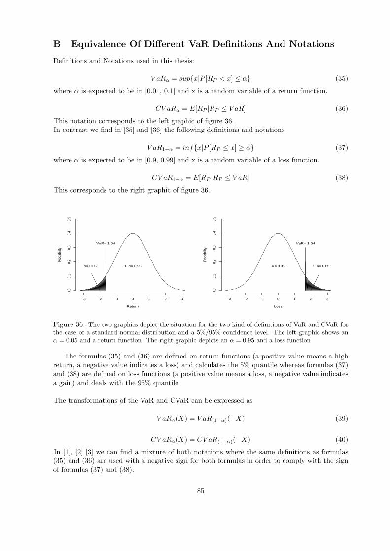
B Equivalence Of Different VaR Definitions And Notations

Definitions and Notations used in this thesis:

V aRα = sup{x|P [RP < x] ≤ α} (35)

where α is expected to be in [0.01, 0.1] and x is a random variable of a return function.

CV aRα = E[RP |RP ≤ V aR] (36)

This notation corresponds to the left graphic of figure 36.In contrast we find in [35] and [36] the following definitions and notations

V aR1−α = inf{x|P [RP ≤ x] ≥ α} (37)

where α is expected to be in [0.9, 0.99] and x is a random variable of a loss function.

CV aR1−α = E[RP |RP ≤ V aR] (38)

This corresponds to the right graphic of figure 36.

Return

Prob

abilit

y

−3 −2 −1 0 1 2 3

0.0

0.1

0.2

0.3

0.4

0.5

α= 0.05 1−α= 0.95

VaR= 1.64

Loss

Prob

abilit

y

−3 −2 −1 0 1 2 3

0.0

0.1

0.2

0.3

0.4

0.5

1−α= 0.05α= 0.95

VaR= 1.64

Figure 36: The two graphics depict the situation for the two kind of definitions of VaR and CVaR forthe case of a standard normal distribution and a 5%/95% confidence level. The left graphic shows anα = 0.05 and a return function. The right graphic depicts an α = 0.95 and a loss function

The formulas (35) and (36) are defined on return functions (a positive value means a highreturn, a negative value indicates a loss) and calculates the 5% quantile whereas formulas (37)and (38) are defined on loss functions (a positive value means a loss, a negative value indicatesa gain) and deals with the 95% quantile

The transformations of the VaR and CVaR can be expressed as

V aRα(X) = V aR(1−α)(−X) (39)

CV aRα(X) = CV aR(1−α)(−X) (40)

In [1], [2] [3] we can find a mixture of both notations where the same definitions as formulas(35) and (36) are used with a negative sign for both formulas in order to comply with the signof formulas (37) and (38).

85

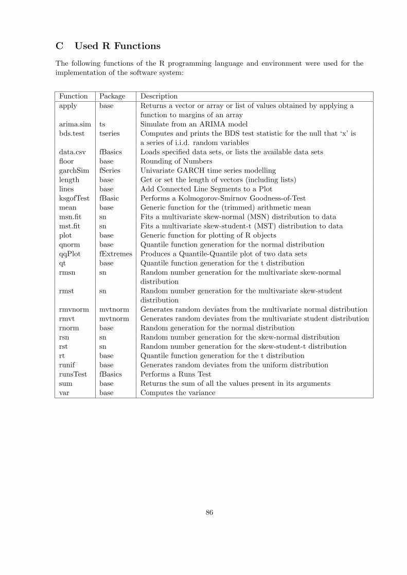
C Used R Functions

The following functions of the R programming language and environment were used for theimplementation of the software system:

Function Package Descriptionapply base Returns a vector or array or list of values obtained by applying a

function to margins of an arrayarima.sim ts Simulate from an ARIMA modelbds.test tseries Computes and prints the BDS test statistic for the null that ‘x’ is

a series of i.i.d. random variablesdata.csv fBasics Loads specified data sets, or lists the available data setsfloor base Rounding of NumbersgarchSim fSeries Univariate GARCH time series modellinglength base Get or set the length of vectors (including lists)lines base Add Connected Line Segments to a PlotksgofTest fBasic Performs a Kolmogorov-Smirnov Goodness-of-Testmean base Generic function for the (trimmed) arithmetic meanmsn.fit sn Fits a multivariate skew-normal (MSN) distribution to datamst.fit sn Fits a multivariate skew-student-t (MST) distribution to dataplot base Generic function for plotting of R objectsqnorm base Quantile function generation for the normal distributionqqPlot fExtremes Produces a Quantile-Quantile plot of two data setsqt base Quantile function generation for the t distributionrmsn sn Random number generation for the multivariate skew-normal

distributionrmst sn Random number generation for the multivariate skew-student

distributionrmvnorm mvtnorm Generates random deviates from the multivariate normal distributionrmvt mvtnorm Generates random deviates from the multivariate student distributionrnorm base Random generation for the normal distributionrsn sn Random number generation for the skew-normal distributionrst sn Random number generation for the skew-student-t distributionrt base Quantile function generation for the t distributionrunif base Generates random deviates from the uniform distributionrunsTest fBasics Performs a Runs Testsum base Returns the sum of all the values present in its argumentsvar base Computes the variance

86

D Description Of The Portfolio Optimization System

It was our intension to do all the calculations on a common hard-/software system in order tomake the analysis as useful for practical applications as possible and easy for future extensions.This justifies the following system:

• The system runs on current personal computers (3GHz clock cycles, 1GB memory). Wedon’t assume the availability of a supercomputer or pc-cluster.

• As software components we use R as front-end application and for some small calculationsand an optimizer module written in Fortran77.

We will now describe how we have designed the system for portfolio optimization. The op-timizer is written in Fortran77 which can be executed directly from R. The full system works asfollows (see figure 37): R calls the optimization routine DONLP2 and gives the needed data (idof optimization method, asset returns, expected return of portfolio) as parameter to the opti-mizer. The optimizer itself calls several subroutines that define the objective function, equalityconstraints and inequality constraints and all of its gradients. In case that it is not possible todefine analytic gradient functions, we have implemented a numerical gradient function.

Asset return data,Risk measure ID

RDONLP2

Optimizer

Objective Function f

Equality Constraint h1

Inequality Constraint g1

Optimal weights

x

f(x)x

g1(x)

x

h1(x)

R Fortran77

Figure 37: Schema of the dependencies of the optimization process.

Our intension is to develop a general purpose system that can easily be installed and ex-tended. For this reason we have chosen a general non-linear optimizer that can be applied toany kind of problems. We are aware that it could be more time efficient to use specializedoptimizers for each problem (e.g. a linear optimizer for the Conditional Value at Risk prob-lem), however we think that the overhead of a general optimizer is negligible in our context.

87

The used optimizer ’DONLP2’ can be downloaded for free from http://ftp.mathematik.tu-darmstadt.de/pub/department/software/opti/ where it is available as Fortran or C implemen-tation. The correct functionality of the optimizer was tested with cross-tests to the optimizerin the R-package ”quadprog” and the optimizer included in Microsoft Excel. In the documen-tation DONLP2 is described as

Purpose:Minimization of an (in general nonlinear) differentiable real function f subject to (in generalnonlinear) inequality and equality constraints g, h.

f(x) = minx∈S

S = {x ∈ Rn : h(x) = 0, g(x) ≥ 0}

Here g and h are vectorvalued functions.Bound constraints are integrated in the inequality constraints g. These might be identified bya special indicator in order to simplify calculation of its gradients and also in order to allow aspecial treatment, known as the gradient projection technique. Also fixed variables might beintroduced via h in the same manner.

Method employed:The method implemented is a sequential equality constrained quadratic programming method(with an active set technique) with an alternative usage of a fully regularized mixed constrainedsubproblem in case of nonregular constraints (i.e. linear dependent gradients in the ”workingset”). It uses a slightly modified version of the Pantoja-Mayne update for the Hessian of theLagrangian, variable dual scaling and an improved Armijo-type stepsize algorithm. Bounds onthe variables are treated in a gradient-projection like fashion. Details can be found in [40] and[41].

88

E Description Of The Excel Optimizer

Optimization in Microsoft Excel begins with an ordinary spreadsheet model. The spreadsheetsformula language functions as the algebraic language used to define the model. Through theSolvers GUI, the user specifies an objective and constraints by pointing and clicking with amouse and filling in dialog boxes. The Solver then analyzes the complete optimization modeland produces the matrix form required by the optimizers. The optimizers employ the simplex,generalized-reduced-gradient, and branch-and-bound methods to find an optimal solution andsensitivity information. The solver uses the solution values to update the model spreadsheetand provides sensitivity and other summary information on additional report spreadsheets.

Detailed information about the methods applied in the optimizer included in MicrosoftExcel are given by Fylstra et al [22].

89

F Description Of Various Hedge Fund Styles

This section lists and explains some common hedge fund strategies. The strategies are takenfrom [6] and the respective volatility classification from the webpage www.magnum.com.

• Convertible Arbitrage. Expected Volatility: LowAttempts to exploit anomalies in prices of corporate securities that are convertible intocommon stocks (convertible bonds, warrants and convertible preferred stocks). Convert-ible bonds tends to be under-priced because of market segmentation; investors discountsecurities that are likely to change types: if the issuer does well, the convertible bondbehaves like a stock; if the issuer does poorly, the convertible bond behaves like distresseddebt. Managers typically buy (or sometimes sell) these securities and then hedge part orall of the associated risks by shorting the stock. Delta neutrality is often targeted. Over-hedging is appropriate when there is concern about default as the excess short positionmay partially hedge against a reduction in credit quality.

• Dedicated Short Bias. Expected Volatility: Very HighSells securities short in anticipation of being able to re-buy them at a future date at alower price due to the managers assessment of the overvaluation of the securities, or themarket, or in anticipation of earnings disappointments often due to accounting irregu-larities, new competition, change of management, etc. Often used as a hedge to offsetlong-only portfolios and by those who feel the market is approaching a bearish cycle.

• Emerging Markets. Expected Volatility: Very HighInvests in equity or debt of emerging (less mature) markets that tend to have higher infla-tion and volatile growth. Short selling is not permitted in many emerging markets, and,therefore, effective hedging is often not available, although Brady debt can be partiallyhedged via U.S. Treasury futures and currency markets.

• Long/Short Equity. Expected Volatility: LowInvests both in long and short equity portfolios generally in the same sectors of the market.Market risk is greatly reduced, but effective stock analysis and stock picking is essential toobtaining meaningful results. Leverage may be used to enhance returns. Usually low or nocorrelation to the market. Sometimes uses market index futures to hedge out systematic(market) risk. Relative benchmark index is usually T-bills.

• Equity Market Neutral. Expected Volatility: LowHedge strategies that take long and short positions in such a way that the impact of theoverall market is minimized. Market neutral can imply dollar neutral, beta neutral orboth.

– Dollar neutral strategy has zero net investment (i.e., equal dollar amounts in longand short positions).

– Beta neutral strategy targets a zero total portfolio beta (i.e., the beta of the longside equals the beta of the short side). While dollar neutrality has the virtue ofsimplicity, beta neutrality better defines a strategy uncorrelated with the marketreturn.

Many practitioners of market-neutral long/short equity trading balance their longs andshorts in the same sector or industry. By being sector neutral, they avoid the risk ofmarket swings affecting some industries or sectors differently than others.

90

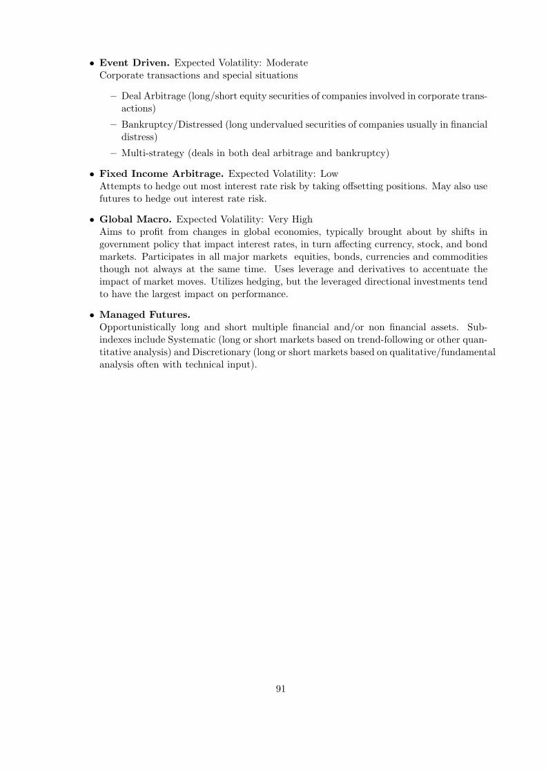
• Event Driven. Expected Volatility: ModerateCorporate transactions and special situations

– Deal Arbitrage (long/short equity securities of companies involved in corporate trans-actions)

– Bankruptcy/Distressed (long undervalued securities of companies usually in financialdistress)

– Multi-strategy (deals in both deal arbitrage and bankruptcy)

• Fixed Income Arbitrage. Expected Volatility: LowAttempts to hedge out most interest rate risk by taking offsetting positions. May also usefutures to hedge out interest rate risk.

• Global Macro. Expected Volatility: Very HighAims to profit from changes in global economies, typically brought about by shifts ingovernment policy that impact interest rates, in turn affecting currency, stock, and bondmarkets. Participates in all major markets equities, bonds, currencies and commoditiesthough not always at the same time. Uses leverage and derivatives to accentuate theimpact of market moves. Utilizes hedging, but the leveraged directional investments tendto have the largest impact on performance.

• Managed Futures.Opportunistically long and short multiple financial and/or non financial assets. Sub-indexes include Systematic (long or short markets based on trend-following or other quan-titative analysis) and Discretionary (long or short markets based on qualitative/fundamentalanalysis often with technical input).

91

G References

References

[1] Acerbi C., Nordio C., Sirtori C., 2001: Expected Shortfall as a Tool for Financial RiskManagement.www.gloriamundi.com

[2] Acerbi C., Tasche D., 2001: Expected Shortfall: a natural coherent alternative to value atriskwww.gloriamundi.com

[3] Acerbi C., Tasche D., 2001: On the Coherence of Expected Shortfall.www.gloriamundi.com

[4] Albrecht P., 2003: Risk MeasuresContribution prepared for: Encyclopedia of Actuarial ScienceJohn Wiley & Sons

[5] Alexander C., 2001: Market modelsJohn Wiley &Sons

[6] Amenc N., Martellini L., 2002: The Brace New World of Hedge Fund IndexesWorking Paper

[7] Artzner P., Delbaen F., Eber J.-M., Heat D., 1999: Coherent measures of riskMathematical Finance 9, pp. 203-228

[8] Belaire-Franch, J., Contrras-Bayarri D., 2002: The BDS Test: A Practioner’s GuideJournal of Applied Econometrics 17, pp. 691-699

[9] Bernoulli D., 1738: Exposition of a new theory on the measurement of risk.

[10] Bollerslev T., 1986: Generalized Autoregressive Conditional Heteroscedasticity.Journal of Econometrics

[11] Brock W., Dechert W.D., Scheinkman J., 1987: A Test for Independence Based on theCorrelation Diemension.University of Wisconsin Working Paper No. 8702

[12] Cheklov A., Uryasev S., Zabarankin M., 2003: Portfolio Optimization With DrawdownConstraints.Working Paper

[13] Cheridito P, Delbaen F., Kupper M., 2003: Coherent and convex risk measures for boundedcadlag˙

[14] Conover W.J., 1999: Practical Nonparametric Statistics.John Wiley & Sons, Inc

[15] De Giorgi E., 2002: A Note on Portfolio Selctions under Various Risk Measures.Working Paper Series ISSN 1424-0459

92

[16] Dembo R., King A., 1992: Tracking Models and the Optimal Regret Distribution in AssetLocation.Applied Stochastic Models and Data Analysis 8, pp. 151-157

[17] Dembo R., Freeman A., 2001: The Rules of Risk.John Wiley & Sons, Inc

[18] Elton E., Gruber M., 1995: Modern portfolio theory.John Wiley & Sons, Inc

[19] Embrechts P., Klueppelberg C., Mikosch T., 2002: Modelling Extremal Events.Springer, pp. 290-294

[20] Embrechts P., Hoing A., Juri A., 2003: Using Copulae to bound the Value-at-Risk forfunctions of dependent risks.Finance & Stochastics 7, pp.145-167

[21] Fishburn P., 1977: Mena-risk analysis with risk associated with below-target returns.The Amerian Economic Review 67, pp. 116-126

[22] Fylstra D., Lasdon L., Watson J., Waren A., 1998: Design and Use of the Microsoft ExcelSolverInterfaces 28, pp.29-55

[23] Gaivoronski A., Pflug G., 2000: Value at Risk in Portfolio Optimization

[24] Grinold R., Kahn R., 1999: Active portfolio managemetMcGraw-Hill, p. 99

[25] Huerlimann W., 2001: Conditional Value-at-Risk bounds for Compund Poisson Risks andNormal Appriximation.Working Paper, MPS: Applied mathematics/0201009

[26] Jia J., Dyer S., 1996: A Standard Measure of Risk and Risk-Value ModelsManagement Science 42, pp. 1691-1705

[27] Kritzman M., 1995: The portable financial analyst.The Financial Analysts Journal

[28] Magdon-Ismail M., Atiya A., Pratap A., Abu-Mostafa Y., 2003: On the Maximum Draw-down of a Brownian MotionWorking Paper

[29] Mandelbrot B., 1963: The variation of certain speculative prices.Journal of Business 36, pp. 394-419

[30] Markowitz H., 1959: Portfolio selection: Efficient diversification of investments.John Wiley & Sons

[31] de Moivre A., 1733:

[32] Pedersen C.S., Satchell E., 1998: An extended family of financial risk measuresGeneva Papers on Risk and Insurance Theory 23, pp. 89-117

93

[33] Peijan A., Lopez de Prado M., 2003: Measuring Loss Potential Of Hedge Fund Strategies.Working Paper UBS Wealth Management and Business Banking

[34] Pflug G., 2000: Some Remarks on the value-at-risk and the conditional value-at-risk.Working Paper at Department of Statistics and Decision Support Systems, University ofVienna

[35] Rockafellar R., Uryasev S., 1999: Optimization of Conditional value-at-riskwww.gloriamundi.com

[36] Rockafellar R., Uryasev S., 2002: Conditional value-at-risk for general loss distributionsJournal of Banking & Finance 26 www.gloriamundi.com

[37] Ross S., 1976: The arbitrage theory of capital asset pricing.Journal of Economic Theory, 13, pp. 341-360

[38] Roy A., 1952: Safety Firts and the Holding of Assets.Econometrica 20, pp.431-449

[39] Schneeweiss H., 1967: Entscheidungskriterien bei Risiko.Springer, pp. 113-117

[40] Spellucci P., 1998: An SQP method for general nonlinear programs using only equalityconstrained subproblemsMath. Prog. 82, (1998), pp. 413-448 Physica Verlag, Heidelberg, Germany

[41] Spellucci P., 1998: A new technique for inconsistent problems in the SQP methodMath. Meth. of Oper. Res. 47, pp. 355-400 Physica Verlag, Heidelberg, Germany

[42] Stone B., 1973: A General Class of Three-Parameter Risk Measures.Journal of Finance 28, pp.675-685

[43] Testuri C., Uryasev S., 2002: On Relation Between Expected Regret and Condtional Value-at-Risk.Working Paper, University of Florida www.gloriamundi.com

[44] Uryasev S., 2000: Conditional Value-at-Risk (CVaR): Algorithms and Applications.Working Paper, University of Florida www.ise.ufl.edu/uryasev

[45] Wang S., Young V., Panjier H., 1997: Axiomatic characterization of insurance prices.Insurance: Mathematics and Economics 21, pp. 173 - 183

94

PORTFOLIO OPTIMIZATION WITH HEDGE FUNDS: Conditional …

Documents