Portfolio-optimization by the mean-variance-approachoptimierung.mathematik.uni-kl.de/mamaeusch/... ·  · 2008-03-09Portfolio-optimization by the mean-variance-approach ... over

Portfolio-optimization by the

mean-variance-approach

Elke Korn

Ralf Korn1

MaMaEuSch has been carried out with the partial support of the European Com-munity in the framework of the Sokrates programme. The content does not neces-sarily reflect the position of the European Community, nor does it involve any re-sponsibility on the part of the European Community.

1 University of Kaiserslautern, Department of Mathematics

MaMaEuSch

Management Mathematics for European Schools

http://www.mathematik.uni-kl.de/~mamaeusch/

101

CHAPTER 4 : Portfolio-optimization by the mean-variance-approach

Overview

Keywords - Economy:

- Stocks

- Risk-free bonds

- Portfolio

- Interest and rate of return / yield

- Mean-variance-principle

- Diversification

Keywords – Elementary mathematics:

- Calculus of probabilities: Expected value and empirical variance

- Finding optimal solutions (see Chapter 1)

- Calculation of interest

- Power(s) and real power

- The Eularian number e

- Inequalities

- Arithmetic average

- Vectors and matrices

Content

- 4.1 Asset management service and portfolio-optimization

- 4.2 Discussion: The portfolio-problem of the Windig Company

- 4.3 Background: Stock terms and definitions, basic principles and history

- 4.4 Basic principles of mathematics: Calculation of interest

- 4.5 Continuation of discussion: Assessment of stock prices

- 4.6 Basic principles of mathematics: Chance, expected value and empirical variance

- 4.7 Continuation of discussion: Balance between risk and profit

- 4.8 Basic principles of mathematics: The mean-variance-approach

- 4.9 Continuation of discussion: Less risk, please! – Optimization from a new standpoint

- 4.10 Summary

- 4.11 Portfolio-optimization: Critique on mean-variance-approach and current research as-

pects

- 4.12 Further exercises

Chapter 4 guidelines

The main goal of this chapter is to introduce the problem of the optimal investment in securities

within the mean-variance-approach according to H. Markowitz. Most of all, in case of an invest-

ment problem with two or three securities we should develop a graphical solution method (similar

102

to that in Chapter 1) which can be employed during class instruction. At the same time one can in

a natural way introduce calculus of probabilities as a mathematical model for chance and uncer-

tainty of the future events.

Some extensive preparation is required in order to cover all the material, depending on the stu-

dents' state of knowledge. It is summarized in each section of this chapter. Thus in Section 4.1

we will by means of an example introduce the problem of optimal investment of capital, namely

the portfolio-optimization. In sections 4.2/5/7/9 we will, while analyzing a portfolio-problem of a

fictitious company, work on the main determinants of the portfolio-optimization, namely profit

(modelled by means of expected value of the rate of return on investment) and risk (modelled by

means of the empirical variance of the rate of return on investment). Moreover we will introduce

the graphical solution method for the portfolio-problem in the case of two to three securities.

In order to be able to handle these sections, economic terms such as rate of return, portfolio

and stocks (see Section 4.3), as well as mathematical knowledge of calculation of interest (see

Section 4.4), as well as calculus of probabilities (see Section 4.6), will be needed.

Depending on the previous knowledge of the students, chapters 4.4 and 4.6 can be skipped.

However Section 4.6 can be used as a short introduction to the calculus of probabilities, which is

here specific to the modern application of "financial mathematics". In chapters 6 and 7 this intro-

duction will be expanded, in fact in any case in which the applications of financial mathematics

utilize the appropriate auxiliary means of the calculus of probabilities. Such an introduction is also

appropriate because in general opinion only few things are as strongly associated with the terms

uncertainty and coincidence as stock prices.

Section 4.8 presents the theoretical principles of the mean-variance-approach according to

Markowitz, firstly in case of an investment in two or three securities, and then in its generality, for

which H. Markowitz was awarded a 1990 Nobel Prize for contributions to economic science. The

first two parts of the section can be, independently of the other sections in this chapter, discussed

with students who possess the basic knowledge of probability theory. The last part of this Chapter

can be most certainly worked out only with very advanced students, and serves as background

information. A very important aspect of Section 4.8 is the diversification principle, which sup-

ports the philosophy of the investment in different goods. An outlook on the current mathematical

methods of the portfolio-optimization will be provided in Section 4.11.

The introduction to the common probability distribution of random variables, as well as the terms

covariance and correlation, is not always possible due to the short time frame of the class. One

can therefore introduce a skimmed version of the mean-variance-approach in which it is possible

to make a risk-free investment (cash, savings account) or go for a risky alternative (e.g. stocks,

stock funds). In Section 4.6 one can discard the common distribution, covariance and correlation.

However, one cannot then effectively present the diversification effect in Section 4.8.

Due to the presence of stock market in the media, in certain parts of this and the following chap-

ter we have included open exercises which involve TV, Internet and appropriate magazines and

journals.

4.1 Asset management service and portfolio-optimization

Good investment – a fictitious experience report

Design student Katerina Schmalenberger* (*imaginary) won 1 million € in the quiz show "Who

wants to be a millionaire?" by means of careful planning and a bit of luck. Ms Schmalenberger

does not want to hide the money under her mattress because first of all that is no safe place for it

and secondly in that way it will not bring her any interest. Likewise she does not want to put the

money on her savings account because there she will presently get interest of merely 1 % per

year, which is simply too little.

103

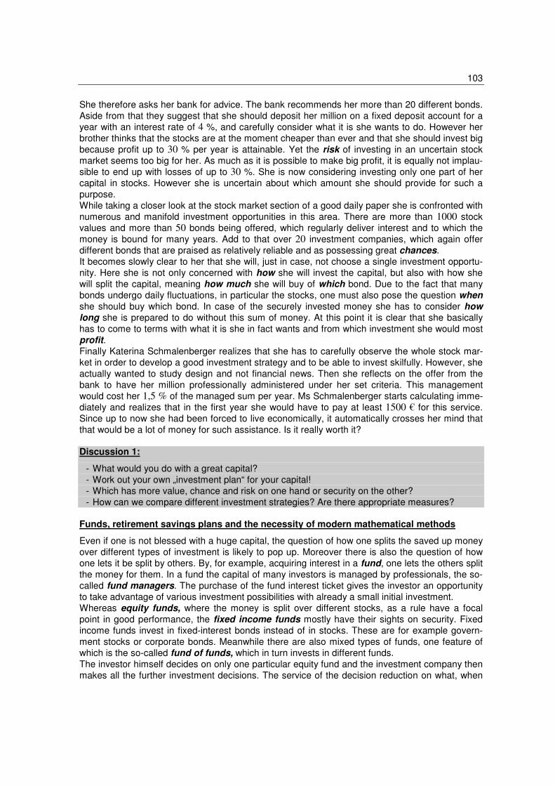
She therefore asks her bank for advice. The bank recommends her more than 20 different bonds.

Aside from that they suggest that she should deposit her million on a fixed deposit account for a

year with an interest rate of 4 %, and carefully consider what it is she wants to do. However her

brother thinks that the stocks are at the moment cheaper than ever and that she should invest big

because profit up to 30 % per year is attainable. Yet the risk of investing in an uncertain stock

market seems too big for her. As much as it is possible to make big profit, it is equally not implau-

sible to end up with losses of up to 30 %. She is now considering investing only one part of her

capital in stocks. However she is uncertain about which amount she should provide for such a

purpose.

While taking a closer look at the stock market section of a good daily paper she is confronted with

numerous and manifold investment opportunities in this area. There are more than 1000 stock

values and more than 50 bonds being offered, which regularly deliver interest and to which the

money is bound for many years. Add to that over 20 investment companies, which again offer

different bonds that are praised as relatively reliable and as possessing great chances.

It becomes slowly clear to her that she will, just in case, not choose a single investment opportu-

nity. Here she is not only concerned with how she will invest the capital, but also with how she

will split the capital, meaning how much she will buy of which bond. Due to the fact that many

bonds undergo daily fluctuations, in particular the stocks, one must also pose the question when

she should buy which bond. In case of the securely invested money she has to consider how

long she is prepared to do without this sum of money. At this point it is clear that she basically

has to come to terms with what it is she in fact wants and from which investment she would most

profit.

Finally Katerina Schmalenberger realizes that she has to carefully observe the whole stock mar-

ket in order to develop a good investment strategy and to be able to invest skilfully. However, she

actually wanted to study design and not financial news. Then she reflects on the offer from the

bank to have her million professionally administered under her set criteria. This management

would cost her 1,5 % of the managed sum per year. Ms Schmalenberger starts calculating imme-

diately and realizes that in the first year she would have to pay at least 1500 € for this service.

Since up to now she had been forced to live economically, it automatically crosses her mind that

that would be a lot of money for such assistance. Is it really worth it?

Discussion 1:

- What would you do with a great capital?

- Work out your own „investment plan“ for your capital!

- Which has more value, chance and risk on one hand or security on the other?

- How can we compare different investment strategies? Are there appropriate measures?

Funds, retirement savings plans and the necessity of modern mathematical methods

Even if one is not blessed with a huge capital, the question of how one splits the saved up money

over different types of investment is likely to pop up. Moreover there is also the question of how

one lets it be split by others. By, for example, acquiring interest in a fund, one lets the others split

the money for them. In a fund the capital of many investors is managed by professionals, the so-

called fund managers. The purchase of the fund interest ticket gives the investor an opportunity

to take advantage of various investment possibilities with already a small initial investment.

Whereas equity funds, where the money is split over different stocks, as a rule have a focal

point in good performance, the fixed income funds mostly have their sights on security. Fixed

income funds invest in fixed-interest bonds instead of in stocks. These are for example govern-

ment stocks or corporate bonds. Meanwhile there are also mixed types of funds, one feature of

which is the so-called fund of funds, which in turn invests in different funds.

The investor himself decides on only one particular equity fund and the investment company then

makes all the further investment decisions. The service of the decision reduction on what, when

104

and how the investment will be made costs a yearly percentage charge fee, or there is another

option, namely to pay the asset-based fees on the purchase price of the fund in the very begin-

ning.

Even if one builds pension funds by means of a retirement savings plan, one hands the others the

work (or task) of dividing the money. Within the retirement savings plan the terms "long term in-

vestment" and "security" become very important. As a rule a type of insurance (e.g. in the event

of death) is included. This means then that the pension insurer splits the money primarily across

fixed-interest securities or funds or perhaps in a convenient insurance, and therefore invests less

in stocks.

Within an equity fund the associated capital investment company divides often very big capital,

comprised of that of all buyers, from particular standpoints, into different stocks. In this way some

investment companies buy only European stocks and moreover only those which have the big-

gest growing potential; or only Asian stocks, and in fact only those which currently bring most

security. After this pre-selection there are then often only approximately 30 to 50 stocks left over

which the capital will be divided. Based on business data and conditions for, e.g. security, the

desired rate of return or the structuring of the fund, the portfolio, namely the investment, will be

optimally divided by the managers. Seen algebraically, at the bottom line, the result is a highly

multidimensional optimization task with (mostly non-linear) side conditions (see Chapter 1 1), e.g.

in the form

Determining optimal investment strategies: Portfolio-optimization

The distribution of a capital over different investment options is called a portfolio. Determining

the optimal investment strategy employed by the investor, meaning the decision on how many

shares of which security they should hold in order to maximize their profit from the final capital

X(T) in the planning horizon T, is in financial mathematics called portfolio-optimization. Here we

have to pay attention that this optimization problem exhibits, aside from its ordinary quantitative

and selective criteria („How many shares of which security?“), a temporal dimension as well

(„when?“). With this in mind one has to continuously make decisions. This is why we are dealing

in general with a so-called dynamic optimization problem.

In this chapter, however, we will observe only models and problems in which one can do without

the temporal element of the decision problem. This is due to the fact that it will deal with a one-

period-approach in which it will be decided on the distribution of the capital into different bonds

only at the beginning of the investment period. This decision will not be revised anymore before

the end of the investment period. The further handling of the portfolio-problem (in other words the

problem of locating an optimal investment strategy) in its generality requires complicated alge-

braic methods such as the stochastic control theory. We will therefore here basically concentrate

on presenting the solution to the simpler portfolio problems and only more closely study the one-

period-model according to Markowitz.

4.2 Discussion: The portfolio-problem of the Windig Company

The Windig Company* (*imaginary), located on the North Sea, has been manufacturing wind

energy plants in middle watt range for ten years. Their hurricane-proof wind turbines have in the

meantime had a big break with farms in isolated locations. The streak of successes of this medio-

cre company is not to be neglected and good labor in this field is very much in demand. Therefore

maximize profit1 + profit2 +…+profit50

Subject to invested capital with weak fluctuation

stock share ≥ 50%

105

the director of the company decided to organize internal retirement pension supplement for his

200 employees. Due to the fact that he is not very familiar with the concept of pension, he invited

the team from "Clever Consulting" to come to his wind energy domicile for a few days. While

drinking tea with cream and with no view out the window because it's storming and raining as it

often does, Selina, Oliver, Sebastian and Nadine are discussing all that they have found out from

the director.

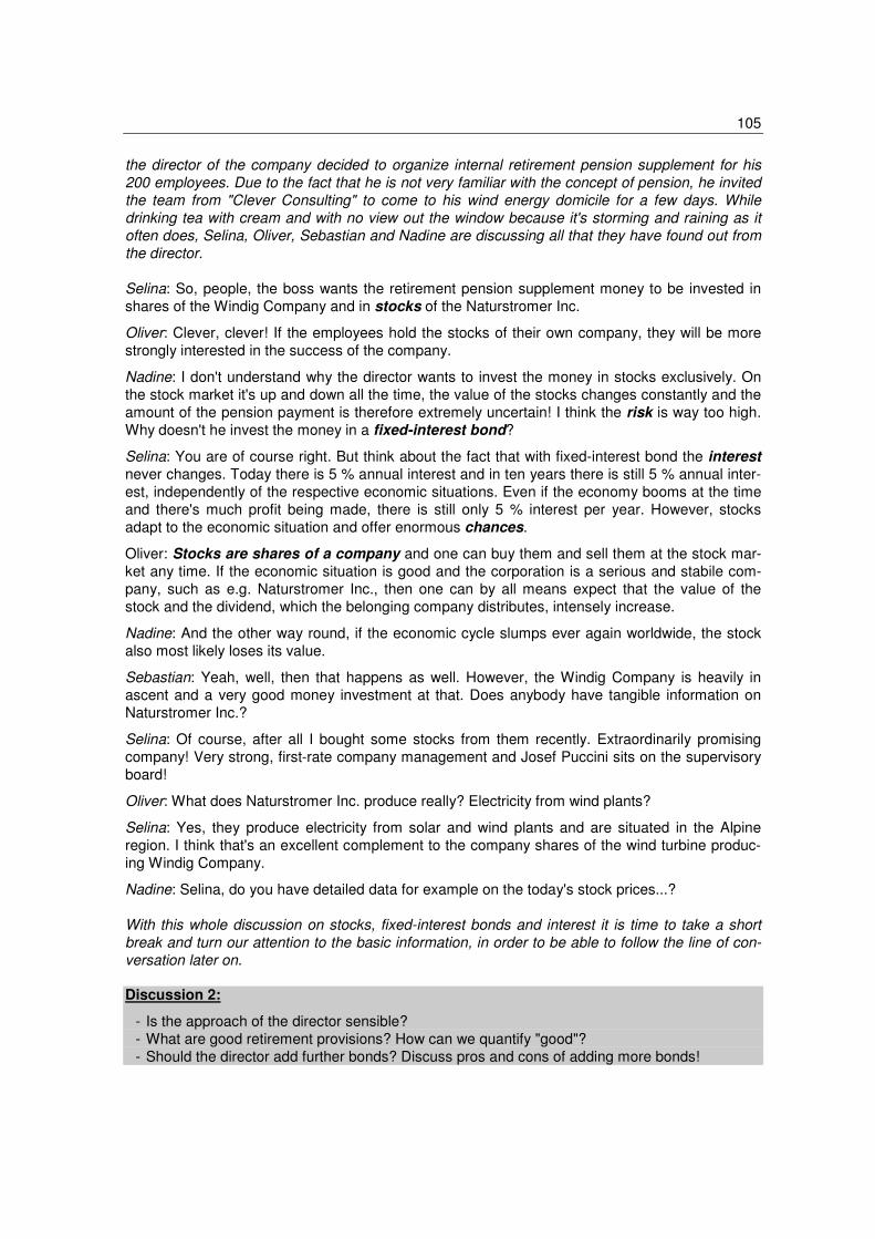
Selina: So, people, the boss wants the retirement pension supplement money to be invested in

shares of the Windig Company and in stocks of the Naturstromer Inc.

Oliver: Clever, clever! If the employees hold the stocks of their own company, they will be more

strongly interested in the success of the company.

Nadine: I don't understand why the director wants to invest the money in stocks exclusively. On

the stock market it's up and down all the time, the value of the stocks changes constantly and the

amount of the pension payment is therefore extremely uncertain! I think the risk is way too high.

Why doesn't he invest the money in a fixed-interest bond?

Selina: You are of course right. But think about the fact that with fixed-interest bond the interest

never changes. Today there is 5 % annual interest and in ten years there is still 5 % annual inter-

est, independently of the respective economic situations. Even if the economy booms at the time

and there's much profit being made, there is still only 5 % interest per year. However, stocks

adapt to the economic situation and offer enormous chances.

Oliver: Stocks are shares of a company and one can buy them and sell them at the stock mar-

ket any time. If the economic situation is good and the corporation is a serious and stabile com-

pany, such as e.g. Naturstromer Inc., then one can by all means expect that the value of the

stock and the dividend, which the belonging company distributes, intensely increase.

Nadine: And the other way round, if the economic cycle slumps ever again worldwide, the stock

also most likely loses its value.

Sebastian: Yeah, well, then that happens as well. However, the Windig Company is heavily in

ascent and a very good money investment at that. Does anybody have tangible information on

Naturstromer Inc.?

Selina: Of course, after all I bought some stocks from them recently. Extraordinarily promising

company! Very strong, first-rate company management and Josef Puccini sits on the supervisory

board!

Oliver: What does Naturstromer Inc. produce really? Electricity from wind plants?

Selina: Yes, they produce electricity from solar and wind plants and are situated in the Alpine

region. I think that's an excellent complement to the company shares of the wind turbine produc-

ing Windig Company.

Nadine: Selina, do you have detailed data for example on the today's stock prices...?

With this whole discussion on stocks, fixed-interest bonds and interest it is time to take a short

break and turn our attention to the basic information, in order to be able to follow the line of con-

versation later on.

Discussion 2:

- Is the approach of the director sensible?

- What are good retirement provisions? How can we quantify "good"?

- Should the director add further bonds? Discuss pros and cons of adding more bonds!

106

4.3 Background: Shares of stock - terms and definitions, basic principles and history

What is a stock?

A corporation is a form of enterprise, much like an Ltd (Limited liability company) or an OHG

(general partnership). A corporation is, among other, characterized by the fact that its basic

capital is divided into many little parts, the shares of stock.

There are shares with constant face value (e.g. 1 € per piece), as well as the so-called real no-

par-value shares, where the holder has a fixed share (e.g. 1/1000000) of the business. In Ger-

many the constant face value stocks are prevalent. However this face value does not play an

important part in determining the actual value of the stock – its price or value. The stock price is

much more a result of the bid and demand for the appropriate stock on the stock market.

The stock market is normally the emporium for stocks. There are stock markets e.g. in Frankfurt,

Stuttgart, London or New York. However not all the stocks are traded on the stock market. There

are also smaller corporations whose stocks can be bought and sold only in specific places, e.g. at

a local savings bank.

The mechanism of bid and demand is determined firstly by two factors:

- the amount of each dividend per share of stock. This is all about an annual distribution of one

part of the business profit to the stock holders (quasi the "stock interest"). The dividend fluctu-

ates according to the profitability of the business and can also completely drop out.

- the (assumed) potential of the stock to achieve further stock price gain which essentially de-

pends on the market estimation of the profitability of the business.

The concept of a "share of stock" originates from Holland (the "native country" of the stock, see

also in historical overview) and is derived from the Latin word „actio“, which approximately means

„enforceable claim“. Accordingly a stock is as a matter of fact something similar to a claim to a

part of a corporation and to a profit belonging to this part. For further legal and economic details,

as well as background information, there will be reference made to the appropriate literature from

the field of business economics.

Why do we need stocks?

Stocks provide an alternative source for big businesses and companies for outside financing (i.e.

borrowing) on capital market. By selling their stocks the corporation obtains the capital in the

amount of the stock price, which as opposed to a loan does not have to be paid back.

As compensation for this paid capital, the stockholders obtain on the one hand yearly dividend

payments, as well as a vote in important business decisions at the stockholders' meeting which

takes place once a year. However, due to the size of the corporation this right to a say in a matter

is limited virtually to individual major stockholders (meaning the owners of very big blocks of

stocks or even the owners of the absolute majority of the stocks) because each stockholder is

entitled to one vote per stock. In this way the minority of the "small" stockholders indeed have the

right to vote, yet the totality of their votes as a rule does not nearly suffice to enforce decisions.

The issue of new stocks or the establishment of a new corporation (e.g. through change of busi-

ness partnership which wants to expand) is often advisable if very big sums of stockholders' eq-

uity are required in order to finance big projects, such as building the first railway line or the foun-

dation of the first overseas trade company, or – as a more current example – building a tunnel

through the English Channel.

Why does one invest in stocks?

Stocks represent a very risky investment opportunity due to the uncertainty of the amount of the

relative yearly dividend, as well as its currency fluctuation. Thus one will purchase stocks only if

one can be assured, for instance based on personal estimate of the future development of the

107

business, of the high dividend payment and strong stock price gain. Summed up these lie high

above the proceeds of a risk-free investment such as fixed term deposit. As a matter of fact the

profit from stock investment, which is as a rule long term (considered over 10 to 20 years), is

despite of slumps which occur now and then still higher than that of the risk-free deposits (see

Chart 4.1, however also Chart 6.1).

0,00

1000,00

2000,00

3000,00

4000,00

5000,00

6000,00

7000,00

8000,00

01.10.199

1

30.09.199

3

30.09.199

5

29.09.199

7

29.09.199

9

28.09.200

1

DA

X (

blu

e)

Chart 4.1 Comparison of the development of the DAX-Index with a 7% return

However generally one should – regardless of how good the personal estimate of the selected

stock(s) is – always get it straight that a stock cannot promise certain profit and that it is still abso-

lutely possible for one to lose part of the invested money. Therefore before each stock investment

one should carefully check if one wants to risk it.

Several important data from the history of the stock:

- 1602: Establishment of the first corporation in the world, the „Vereinigte Ostindische Kom-

panie“, in the Netherlands, for financing an overseas trade company

- End of 17. century: Increase in stock dealing, particularly in England and France

- 1756: Dealing the first German stock, the „Preußische Kolonialgesellschaft“, in Berlin

- 1792: Founding of (the forerunner) of the New Yorker stock market, since 1863 „New York

Stock Exchange“

- 1844: In England it is legally possible to found corporations in all branches of acquisition

- 1884: The first American stock index, the „Railroad Average“, which contains the stocks of

American railroad companies, is quoted

- 1897: The Dow-Jones-Stock Index is determined each trading day

- 1929: Black Friday („stock market crash“) on 25.10.1929 at the New York stock market

- 1959: Issue of the first German people' share (PREUSSAG)

- 1961: Issue of the second German people's share (VW)

- 1987: Black Monday on 19.10.1987, surprisingly rapid collapse on the international stock mar-

kets

- 1988: The German stock index (DAX) is introduced

- 1996: The people's share Deutsche Telekom Inc. goes public

- 1997: The fully electronic trading system Xetra is introduced by the Deutschen Börsen Inc.

- 2000: The DAX reaches the historical all-time high of 8064 points on 7.3.2000

Fixed-interest bonds

As opposed to stocks, the value development of a fixed-interest bond is already determined in

advance. As a rule one sets up a determined sum of money for a specific amount of time and

then obtains interest which was stipulated in advance at regular intervals. At the end of the period

108

of validity of the bond one gets the invested capital back. The examples of fixed-interest bonds

include federal savings bonds, long-term bonds, corporate bonds, state bonds or Pfandbrief.

Moreover fixed deposits of a house bank or an account book can be in a sense considered a

bond.

One often connects the term fixed-interest bond with the term risk-free bond. This is only true

insofar as one considers that the interest payments and the return value are determined in ad-

vance. Yet the „risk-free bonds" are not entirely risk-free, particularly not if we are talking about

business bonds of a ramshackle company or the government bond of an instabile and overdebted

country. Under such circumstances the interest payments, and sometimes even the return on

capital can be omitted. Thanks to the strict rules and thorough control by the supervision of bank-

ing, most of the fixed-interest bonds belonging to the bank are in fact almost risk-free.

Discussion 3:

- Which great corporations are there?

- By means of magazines and Internet try to find out how many stocks were issued by certain

corporations! Calculate, based on the current stock prices, how much money one has to invest

in order to buy up all the stocks! Discuss the meaning of this value!

- Inform yourself on the Internet, in magazines and manuals on the terms stock, bond and obli-

gation.

4.4 Basic principles of mathematics : Calculation of interest

Interest and compounded interest

The bondholder of a fixed-interest bond regularly obtains agreed-upon interest which corresponds

to the respective capital. If the original assets K0 are invested as fixed deposit for a year with

annual return of r %, at the end of the year we get the following closing capital:

( )1

0 0 0;1 1100 100

r rK r K K K

= + ⋅ = ⋅ +

.

If this capital is fixed over several years, then we have to consider that normally the interest is

credited on the account annually, so that there is equally interest on that interest in the aftermath.

The interest on the interest is called compounded interest.

Annual return: A capital of K0 , which is invested as fixed deposit with annual return of r %

throughout n years finally results in the closing capital of:

( ) 0; 1100

nr

K r n K

= ⋅ +

.

Entirely in contrast to this is the concept of short-term financial investment. There is also the pos-

sibility of investing the fixed deposit for a month or even a few days. In this case one has to pay

attention that the interest rate is valid for a full year and accordingly, in case of a short-term in-

vestment, only a part of it will be paid out.

Return in case of a short-term financial investment („Return of less than a year“): Opening

capital of K0, invested for m≤12 months results, in case of an annual return of r%, in closing

capital of:

109

( ) 0; ,1 1100 12

r mK r m K

= ⋅ + ⋅

.

Opening capital of K0, invested for t≤360 (interest-)days, results, in case of an annual return of

r%, in closing capital of:

( ) 0; ,1 1100 360

r tK r t K

= ⋅ + ⋅

.

Incidentally in banking business one month is mostly converted into 30 days and one bank year

consists of 360 days (in fact: interest days).

Aside from the investment or saving interest which one quasi obtains as a reward for relinquish-

ing the capital to the bank, there is one more contrarian perspective. After all at a bank one can

invest money as well as lend it. In the latter case one has to pay the so-called loan interest to the

bank. The situation becomes unfavourable for the borrower if they neither pay back the loan nor

pay interest for the duration of the loan. This interest is added to the loan and demands, in case

of a loan that is stretched over several years, the loan interest itself. The compounded interest

effect increases the debt rapidly. The result are the same formulas as in the case of the fixed

deposit because a loan is indeed the same as a fixed deposit, excepting the fact that one is on

the other side of the transaction.

(→Ex.4.1, Ex.4.2)

Continuous compounding

In a fixed deposit over e.g. three months after the expiry one gets not only their capital back, but

obtains the interest as well. If the interest rate has not changed in the meantime, this whole sum,

in other words the capital plus interest, can be newly invested at the same interest rate over the

same period of time. In this way the compounded interest effect is noticeable already after a short

period of time.

Return in case of a repeated short-term financial investment: Opening capital of K0, j-times

repeated, including the interest invested over respectively m≤12 months results in, in case of an

annual return of r%, in closing capital of:

( ) 0; , 1100 12

jr m

K r m j K

= ⋅ + ⋅

.

Opening capital of K0, j-times repeated, including interest invested over respectively t≤360 (inter-

est-) days results, in case of an annual return of r%, in closing capital of:

( ) 0; , 1100 360

jr t

K r t j K

= ⋅ + ⋅

.

(→Ex.4.3)

Let us take a closer look at an extreme case: A daily allowance is invested 360 times consecu-

tively at the same interest rate. In case of the capital of 5000 €, which is fixed as daily allowance

at the annual interest rate of 4 % and is newly invested every day under the same conditions, we

get 5204,04 € (rounded off) after a year:

( )360

4 14;360,360 5000 1 5204,042305

100 360K

= ⋅ + ⋅ =

.

110

This final amount clearly exceeds the amount of 5200 €, which is obtained if the money is fixed

for a year at the same annual interest rate of 4 %. The interest which is paid out daily and added

to the capital lead by means of the compounded interest to the higher final capital. One could now

divide the time even more closely and introduce an hourly fixed deposit, minute or even second

fixed deposit. We observe that the final capital moves towards a boundary level (i.e. ultimately

hardly anything changes). One then says that the capital continuously pays interest. The capi-

tal of 5000 € that continuously pays interest at an interest rate of 4 % results after a year in the

closing capital of 5204,05 € (rounded off):

( )4

11004 ;1 5000 5204,053871sK e

⋅= ⋅ = ,

whereby e is the Eularian number. This type of return is entirely common in banking circles and

the interest rate is called continuous interest rate. The above formula is true for optional peri-

ods of time t∈[0,∞], where t is measured in years (e.g. 1 1/2 years are t =1,5).

Continuous return: Opening capital of K0, with a continuous interest rate of r%, results after

period of time t in closing capital of:

( ) 0100;

s

s

rt

K r t K e⋅

= ⋅ .

Chart 4.2 Comparison between one-year, half-a-year and continuous return (r=0,2)

When borrowing one has to particularly pay attention to whether the interest is paid continuously

or whether the interest is added to the loan quarterly or yearly. For this reason within the loan

procedure as a rule what is always additionally specified is the effective interest rate. The effec-

tive interest rate is the interest rate which would during the yearly calculation of interest lead to

the same closing payment as the offered interest calculation type (always based on the whole

year). If for example the interest at the given annual interest of r% is added to the capital quar-

terly, one gets the effective annual interest reff % by means of the equation

( ) ( );3 ,4 ;1effK r m K r= ,

one therefore compares

one year

half a year

continous

111

14

0 0

31 1

100 12 100

effrrK K

⋅ + ⋅ = ⋅ +

,

and thus finds

43

1 1 100100 12

eff

rr

= + ⋅ − ⋅

.

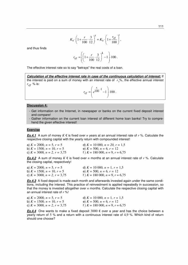
The effective interest rate so to say "betrays" the real costs of a loan.

Calculation of the effective interest rate in case of the continuous calculation of interest: If

the interest is paid on a sum of money with an interest rate of r s%, the effective annual interest

reff % is:

1

100 1 100

s

eff

r

r e⋅

= − ⋅

.

Discussion 4:

- Get information on the Internet, in newspaper or banks on the current fixed deposit interest

and compare!

- Gather information on the current loan interest of different home loan banks! Try to compre-

hend the given effective interest!

Exercise

Ex.4.1 A sum of money K € is fixed over n years at an annual interest rate of r %. Calculate the

respective closing capital with the yearly return with compounded interest!

a) K = 2000, n = 5, r = 5 d) K = 10 000, n = 20, r = 1,5 b) K = 1500, n = 10, r = 5 e) K = 500, n = 6, r = 12

c) K = 3000, n = 2, r = 3,75 f ) K = 180 000, n = 9, r = 6,75

Ex.4.2 A sum of money K € is fixed over n months at an annual interest rate of r %. Calculate

the closing capital, respectively!

a) K = 2000, n = 5, r = 5 d) K = 10 000, n = 1, r = 1,5 b) K = 1500, n = 10, r = 5 e) K = 500, n = 6, r = 12 c) K = 3000, n = 2, r = 3,75 f ) K = 180 000, n = 9, r = 6,75

Ex.4.3 A fixed deposit is made each month and afterwards invested again under the same condi-

tions, including the interest. This practice of reinvestment is applied repeatedly in succession, so

that the money is invested altogether over n months. Calculate the respective closing capital with

an annual interest rate of r %!

a) K = 2000, n = 5, r = 5 d) K = 10 000, n = 1, r = 1,5 b) K = 1500, n = 10, r = 5 e) K = 500, n = 6, r = 12 c) K = 3000, n = 2, r = 3,75 f ) K = 180 000, n = 9, r = 6,75

Ex.4.4 One wants to make a fixed deposit 3000 € over a year and has the choice between a

yearly return of 5 % and a return with a continuous interest rate of 4,9 %. Which kind of return

should one choose?

112

Ex.4.5 For the loan on K € we agreed upon a continuous interest rate of r %. The period of valid-

ity of the loan is n months. Only at the end of this time the amount of the loan including the inter-

est must be counted. Calculate the amount repayable! (Clue: n = 60 makes t = 5.)

a) K = 2000, n = 60, r = 5 d) K = 10 000, n = 1, r = 1,5 b) K = 1500, n = 10, r = 5 e) K = 500, n = 6, r = 12 c) K = 3000, n = 24, r = 3,75 f ) K = 180 000, n = 9, r = 6,75

Ex.4.6 Compare the results in Ex.4.1, Ex.4.2, Ex.4.3 and Ex.4.5, as far as they are comparable!

Ex.4.7 In case of a loan we agreed upon a quarterly calculation of interest with an annual interest

rate of r%. Specify the effective interest rate!

a) r = 5 d) r = 1,5

b) r = 4,2 e) r = 12

c) r = 3,75 f ) r = 6,75

Ex.4.8 Specify the effective interest rate for a continuous interest rate of r %!

a) r = 8 d) r = 7,5

b) r = 0,9 e) r = 6,75

c) r = 3,75 f ) r = 12

Ex.4.9 Specify the formula for the calculation of the effective interest rate with the monthly inter-

est calculation!

4.5 Continuation of the discussion: Assessment of stock prices

If we consider bonds and stocks, Selina is here like a fish in the water and reports with enthusi-

asm elaborately on all the possible details. It is quite amazing which trivia she can remember

while discussing this topic. However she completely forgets to add cream to the strong, bitter tea

in front of her.

Selina: Today in the morning the Naturstromer released a stock in Frankfurt at 47,30 €, that was

really feeble. As it got to 48,10 € at 10 o'clock in Stuttgart, I considered whether to sell my own

stocks and take the profit. Five minutes ago it was in Xetra-Handel at 47,80 € ,... Wow, this tea is

strong!

Nadine: Didn't need to know it in so much detail...

Selina: That's ok. Hier in my newspaper I have a printout of the stock charts for the last three

months. The closing price of the stock is specified on each day:

113

Chart 4.3 (fictitious) stock price of Naturstromer Inc.

Oliver: Holy cow, in August the stock amply went down, and on August 20 it was below 40 € !

Selina: And not even a month later, on September 16, it was above 45 €. Since the change of

supervisory board of the corporation, the stock is again very much in demand!

Nadine: Yeah, there seems to be an upward tendency. Aside from the stock price, do you have

any other information about this stock? Maybe the most recently paid dividend and the dividend

rate of return or something similar?

Selina: The dividend, as well as the dividend rate of return, are inappropriate operating figures

for this stock. At the last general assembly in August it was namely decided that nothing should

be distributed to the stockholders. But not because this company is doing badly, rather because

the cumulative profit should be reinvested. The chances of growth are very big at the time, and so

it pays off to further develop the company. A better operating figure is a value from the newspa-

per in case of which the opening capital K0 invested in this stock can be compared with the capi-

tal which results from the investment over a year:

Three years ago this stock had an annual rate of return of 7.8 %, two years ago that of 8.2 % and

last year it amounted to 8 %. It paid interest very well! A lot more than this wishy-washy 5 % in-

terest on fixed deposit.

Oliver: One could assume that it'll continue to develop like that. I estimate that we can expect an

8 % rate of return for this stock.

Sebastian: But the stock rate of return is anything but safe. The price of the stock and the divi-

dend payment strongly fluctuate and are determined by mere chance.

Selina: But the stock of the Naturstromer Inc. is relatively stabile, quite in contrast to the stock of

Microsaft Inc, that one sinks enormously after each bad stock market day.

0

0_____

K

Kyearoneafterreturnofrateyield

−=

114

Sebastian: Sure, different stocks fluctuate with different intensity. Do we have any indication any-

where as to how much these fluctuate?

Selina: The frequency and intensity of the price fluctuation within a specific time frame is specified

in this newspaper with the measure of volatility. It says here that the Naturstromer stock in the

last 250 days had the volatility of 20 %.

Sebastian: Oh yeah, the volatility! In a bit of a simplified manner, this volatility corresponds to the

standard deviation of the annual rate of return. As a matter of fact, one can work well with this

value!

Oliver: Take a look, the Microsaft Inc. has a volatility of 40 %, i.e. their stock price fluctuates in-

deed a lot more than that of Naturstromer Inc. As opposed to that Vögelchen Milch Inc. has vola-

tility of only 10 %, which means their price mostly changes very little.

Selina: You can forget that stock! You will obtain no stock price gain. On top of everything the

dividend is so low that you can invest your money in a fixed deposit right away. I'd say the rate of

return is significantly below 5 % per year.

Unfortunately at this point we have to interrupt the conversation on different stocks and their mar-

ket chances. We should now find out more about chance in order to be able to understand what

is expected value and variance. Once we are equipped with the knowledge on these basic princi-

ples, we can follow that adjacent expert talks.

Discussion 5:

As addition to the above discussion one can use newspaper reports on the price development of

individual stocks or comments on TV analyses concerning the history and the future of the stock.

Further aspects:

- What all can be incorporated in the assessment of a stock (e.g. certainty, rates of return in the

past, product range of a company, quality of the company management, connection to other

stocks,...)?

- Gather information on the Internet, in manuals and newspaper on which operating figures exist

for stocks!

- Observe the current stock charts in newspaper! Give the estimated value for rates of return

(more than fixed deposit interest?) and volatility (in form of "small", "normal", "very big")!

Exercises

Ex.4.10 Describe both the following three-month stock charts!

115

Chart 4.4 Stock price of Siemens Inc. 2002 Chart 4.5 Stock price of RWE Inc. 2002

Instruction: The 250-day-volatility of Siemens Inc. was indicated on 12.11.2002 at 53,49 %, the

250-day-volatility of RWE Inc. at 28,9 %. Compare these values with price trends!

Ex.4.11 Try to create a fictitious 3-month stock chart for Vögelchen Milch Inc. mentioned in the

course of discussion! Take into consideration the fact that the volatility and the expected rate of

return of this stock are low.

4.6 Basic principles of mathematics: Chance, expected value and variance

On chance

In everyday life there are only few things which are so quickly brought into connection with the

term "chance" as are stocks. Nobody seems to be able to efficiently predict their exact future

values, however now and then it is possible to predict their business trend. We can compare this

to a football game between two teams of different quality, during which we rather count on the

victory of the better team, but we cannot predict it with certainty. Therefore we will also – later –

present the appropriate models for stock prices in which one possibly has a clear opinion on the

business trend of the future development and yet cannot predict the exact price. In such a case

one models the stock price as a result of a chance experiment.

Firstly we should observe, as a classical example of a chance experiment, the result (elementary

event) of a one dice throw. We know exactly that only one of the values 1,2,3,4,5,6 can emerge

as the result. In case of a fair throw for each of these values there should be equal chance of

each one being thrown. In addition we could be interested also in complex events, such as e.g.

throwing an even number on the dice.

In order to describe such an experiment, one needs three things:

- The set Ω of all possible outcomes of the experiment, here thus Ω = 1,2,3,4,5,6.

- The set of all possible events. We will at this point choose the power set of Ω, i.e. the set of

all subsets of Ω, which we will designate with 2Ω =A | A⊆Ω. For the dice example it is 2Ω =1,..., 6, 1,2,...,1,2,3,4,5,6.

- The probability P(A) for each event A⊆Ω , here thus particularly for the elementary events:

P(1)=P(2)=P(3)=P(4)=P(5)=P(6)=1/6.

The set Ω of all possible outcomes describes therefore what one could observe during the execu-

tion of the experiment. An event A⊆Ω represents a type of categorization of the result, e.g.

A=2,4,6 means that an „even number“ was thrown. The possibilities of the dice game arise in

116

the following manner: Since we have six different probable outcomes and every result is equally

probable, the same probability of 1/6 has to be ascribed to each outcome.

- Aside from that we are interested in the consequence X(ω) of the outcome ω∈Ω of the ex-

periment, in this case this is firstly X(ω)=ω, namely the number thrown.

Actually one could imagine a game in which we are not interested in the thrown number but the

derived quantity. If we had e.g. taken part in a bet in which we would have in case of an even

number won 1 € and in case of an odd number lost 1 €, then for us only the outcomes "even" (i.e.

2, 4, 6) and "uneven" (i.e. 1, 3, 5) and their consequence „+1 €“ or „-1 €“ would have been rele-

vant. In such a case it would be true

( )

1, if 2,4,6

1, if 1,3,5X

ωω

ω

+ ∈=

− ∈.

Definition:

a) A (finite) probability space (Ω, P) consists of an non-empty set Ω (with finitely many ele-

ments), the result set, and a probability measure P, i.e. a function P: 2Ω→[0,1], which gives

each event A⊆Ω a number P(A)∈[0,1] and for which it's true:

(P1) ( ) 0P ∅ = and ( ) 1P Ω = .

(P2) ( ) ( ) ( )P A B P A P B∪ = + for A,B⊆Ω with A∩B=∅.

The elements ω∈Ω are called elementary events.

b) A (real-valued) random variable X in (a finite probability space) (Ω, P) is a figure X: Ω→IR.

In this definition we have set certain conditions as far as probability is concerned, which can be

easily comprehended: In this way the probability of an elementary event should always be posi-

tioned between zero and one; the probability "one" will be assigned to the certain event („Some-

thing is happening“) and the probability zero to the impossible event – the empty set.

(→Ex.4.12-15)

Note: Due to the fact that we will here explicitly observe only finite probability spaces, we have

omitted the introduction of the term σ -algebra. As follows, all the conducted observations are e.g.

right for the choice of the power set as σ -algebra. The constraint to finite probability spaces al-

lows for a more simple definition of the probability measure, so that in (P2) only additivity is to be

demanded.

Calculating probability

The definition results in several simple calculation rules for probability:

Calculation rules for probability:

In a finite probability space it is true:

a) For A ⊆ Ω it is true: ( ) ( )A

P A Pω

ω∈

= ∑ ,

i.e. the probability of a subset of Ω results as a sum of the probability of its elements.

b) For A, B ⊆ Ω with A ∩ B = ∅ it is true: P(A ∪ B) = P(A) + P(B).

c) For A, B ⊆ Ω it is true: P(A ∪ B) = P(A) + P(B) − P(A ∩ B).

117

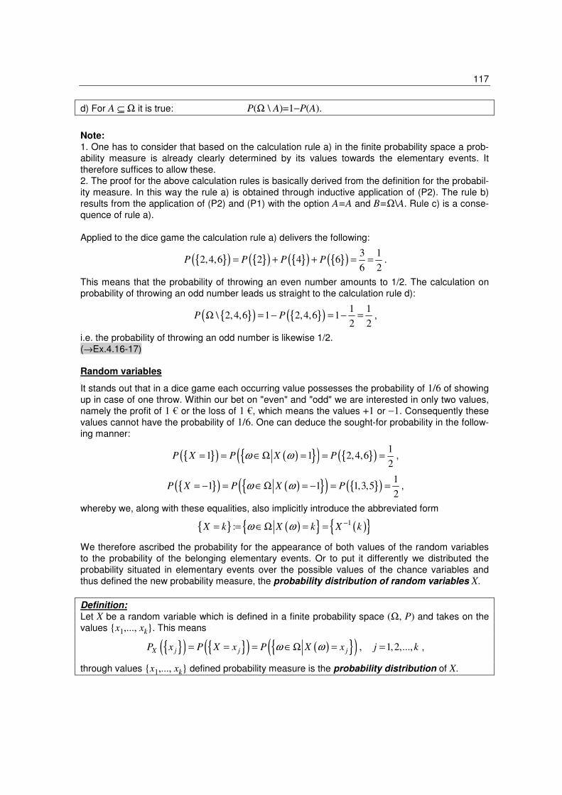
d) For A ⊆ Ω it is true: P(Ω \ A)=1−P(A).

Note:

1. One has to consider that based on the calculation rule a) in the finite probability space a prob-

ability measure is already clearly determined by its values towards the elementary events. It

therefore suffices to allow these.

2. The proof for the above calculation rules is basically derived from the definition for the probabil-

ity measure. In this way the rule a) is obtained through inductive application of (P2). The rule b)

results from the application of (P2) and (P1) with the option A=A and B=Ω\A. Rule c) is a conse-

quence of rule a).

Applied to the dice game the calculation rule a) delivers the following:

( ) ( ) ( ) ( )3 1

2,4,6 2 4 66 2

P P P P= + + = = .

This means that the probability of throwing an even number amounts to 1/2. The calculation on

probability of throwing an odd number leads us straight to the calculation rule d):

( ) ( )1 1

\ 2,4,6 1 2,4,6 12 2

P PΩ = − = − = ,

i.e. the probability of throwing an odd number is likewise 1/2.

(→Ex.4.16-17)

Random variables

It stands out that in a dice game each occurring value possesses the probability of 1/6 of showing

up in case of one throw. Within our bet on "even" and "odd" we are interested in only two values,

namely the profit of 1 € or the loss of 1 €, which means the values +1 or −1. Consequently these

values cannot have the probability of 1/6. One can deduce the sought-for probability in the follow-

ing manner:

( ) ( ) ( ) ( )1

1 1 2,4,62

P X P X Pω ω= = ∈Ω = = = ,

( ) ( ) ( ) ( )1

1 1 1,3,52

P X P X Pω ω= − = ∈Ω = − = = ,

whereby we, along with these equalities, also implicitly introduce the abbreviated form

( ) ( ) 1:X k X k X kω ω −= = ∈Ω = =

We therefore ascribed the probability for the appearance of both values of the random variables

to the probability of the belonging elementary events. Or to put it differently we distributed the

probability situated in elementary events over the possible values of the chance variables and

thus defined the new probability measure, the probability distribution of random variables X.

Definition:

Let X be a random variable which is defined in a finite probability space (Ω, P) and takes on the

values x1,..., xk. This means

( ) ( ) ( ) ( ) , 1,2,...,X j j jP x P X x P X x j kω ω= = = ∈Ω = = ,

through values x1,..., xk defined probability measure is the probability distribution of X.

118

Discussion 5:

At this point – before we introduce expected value and variance – we can discuss how one could

summarize in single ratios the information which contains probability distribution over a real

chance variable. Possible alternatives to expected value can be e.g. median (mean value of the

value range of X) or the mode (the most probable value for X).

Expected values

As a rule the random variables indicate the values which are of more interest to us than the de-

tailed outcome of the chance experiment, such as for example the profit or loss of 1 € in the

"even-odd" bet. If we play this chance game more often we want to additionally know if we will in

the long run make profit or if we are dealing with a game in which we will encounter losses. In

this dice game it seems that profit and loss are in balance, assuming that the dice is really fair.

This is why we tend to allocate to this game a profit / loss value of 0.

It gets even more thrilling in telephone games which are hosted several times daily on certain TV

channels. Does it really pay off to invest e.g. 1,90 € in a telephone call each day if we are at-

tracted by a profit of 500 €? In this case our random variable X would take on the values X = -

1,90 and X = 498,10. Can one assign likewise a type of profit / loss expectancy to these random

variables?

In general one random variable is distinctly determined through the designation of the possible

values and their belonging probability distribution. If a chance variable takes on more values, one

is interested in the summary of its performance. Is there maybe a type of average value around

which the possible values of the random variable are distributed?

One could e.g. choose the arithmetic average of all possible values. However this has signifi-

cance only in case of equipartition over all values (i.e. all possible values of the chance variables

are accepted with equal probability). Yet if the individual outcomes are more probable than oth-

ers, then one will, while frequently repeating the experiment, as a rule more often observe them

as an occurring result than less probable outcomes. In order to allow for this, one creates an av-

erage weighted with probability of the individual values of the chance variables, i.e. the expected

value or expectation:

Definition:

Let X be a random variable in a finite possibility space (Ω, P) which takes on the values x1, ..., xk. Ω has n elements. This means the value

( ) ( ) ( )1 1

n k

i i j j

i j

E X X P x pω ω= =

= =∑ ∑

is the expected value of X, whereby ( )j X jp P x= .

We should consider that one can obtain the expected value by calculating the average of the

possible values xj of the chance variables weighted by the belonging probability distribution of X.

It can be also obtained by calculating the average of the values belonging to the elementary

events X(ωi), weighted by the original probability of the elementary events.

In the "even-odd" game we obtain:

( ) ( ) ( ) ( )1 1 1 1X XE X P X P X= − ⋅ = − + ⋅ =

119

( ) ( ) ( ) ( )1 1 1 1 1 1 1

1 1 1 1 1 1 16 6 6 6 6 6 6

= − ⋅ + ⋅ + − ⋅ + ⋅ + − ⋅ + ⋅ + − ⋅ .

1 1

1 1 02 2

= − ⋅ + ⋅ =

This is exactly what we presumed. In a classical dice example we reach:

( )6

1

1 213,5

6 6i

E X i=

= ⋅ = =∑ .

Although this is a very simple example, one can in this way clear up many issues:

- The expected value has to be a possible value (one can after all not throw 3,5!) and is thus no

value that can be “expected to occur".

- If one observes only some few attempts, the expected value will as a rule not be concordant

with the arithmetic average of the observed attempt outcomes.

- If however the number of the attempt repetitions is large, the arithmetic average of the ob-

served results will only slightly deviate from expected value. This is a type of consequence

from the (strict) law of large numbers, which we will learn later on.

Let us return to the telephone lottery in which the determination of the probability distribution is

still applied. In the following deliberation we will assume that based on the high telephone costs

only 5000 people take part in the game and they all have the same probability of winning. Since

only one person can win, it is true

1

( 498,10)5000

P X = = and ( )4999

1,905000

P X = − = .

For this reason the expected value is

( ) ( )4999 1

1,90 498,10 1,805000 5000

E X = − ⋅ + ⋅ = − .

If one played these telephone games very often, on a continuing basis, one would have in each

individual game on average a loss of 1,80 €. In the following chart we simulated frequent playing

and calculated the respective average costs per game. We see that the more often one takes

part, as a rule the closer the average costs are positioned in case of expectation.

0,000,100,200,300,400,500,600,700,800,901,001,101,201,301,401,501,601,701,801,90

0 100.000 200.000 300.000 400.000 500.000

Anzahl der Teilnahmen

Du

rch

sc

hn

itts

ko

ste

n

Chart 4.6 Simulated average costs in a lottery game

Avera

ge

costs

Number of participations

120

Calculation rules for expectation

Similarly to the probability, there is also a calculation rule for expected values, which results di-

rectly from the definition of the expectation:

Rules for calculation with expectation:

Let X and Y be the random variables in the finite probability space (Ω, P). It is then true:

a) E(X + Y) = E(X) + E(Y).

b) It is true for all ω∈Ω X(ω) ≥ Y(ω), thus also E(X) ≥ E(Y).

c) If c∈IR, it is true that E(c⋅ X) = c⋅ E(X).

(→Ex.4.18-20)

Variance and standard deviation

The expected value alone still does not provide us with enough insight. After all we have discov-

ered by employing an example of the dice game that it is no "anticipated value" but that it merely

results from the theoretical average of the outcomes of the frequent attempt repetitions. The ex-

pected value is a good indicator of the next outcome of the chance experiment only if one knows

that the results as a rule do not strongly deviate from the expected value. In order to be able to

evaluate that we need the terms variance and standard deviation. The variance (as well as

standard deviation) is a measure for the dispersion of chance variables around the expected

value.

Definition:

Let X be a random variable in a finite probability space (Ω, P). In this case variance of X, Var(X),

is defined as

( ) ( )( )2Var X E X E X= − .

The value

( ) ( )X Var Xσ =

is called the standard deviation of X.

We want to comment on this definition as follows:

- The variance measures the average quadratic distance of the chance variable to its expected

value. This on the one hand prevents the positive and negative distances from cancelling each

other (if we observed the average distance, we would namely get: E((X - E(X))) = E(X) – E(X)

= 0). On the other hand this means that the variance is measured in other units than the ex-

pected value. However the standard deviation is then again measured in right units.

- A small variance indicates that one will as a rule obtain attempt results which are positioned

close to the expected value.

- Along with X is (X – E(X))² also again a random variable in (Ω, P), which finally takes on many

values. This guarantees that the variance as expected value in the context of our definition ex-

ists in the first place.

Calculation rules for variance

Before we consider the examples, let us summarize several simple calculation rules with which

we can more easily calculate variance and standard deviance:

Calculation rules for the variance:

121

Let X be a random variable in a finite probability space (Ω, P).

a) ( ) ( ) ( )( )22

Var X E X E X= − .

b) If c∈ IR , it is thus true that: ( ) ( )2Var c X c Var X⋅ = ⋅ , ( ) ( )Var X c Var X+ =

These rules result directly from the definition of variance. By means of the rule a) and the ex-

pected value already calculated for the dice throwing, we obtain the following for the variance and

the standard deviation of the one-time throw:

( ) ( ) ( )( ) ( )6

2 22 2 7 3516 2 12

1i

Var X E X E X i=

= − = ⋅ − =

∑ ,

( )35

1,7112

Xσ = ≈ .

Even if this is algebraically not entirely correct, one can by means of standard deviation get the

first glimpse of the outcome of a chance experiment. Therefore as a rule quite many results will

be positioned in the area of expected value plus/minus standard deviation. In our case of the dice

experiment this would be the area between 3,5 - 1,71 = 1,79 and 3,5 + 1,71 = 5,21, which would

correspond approximately to our idea of dice throwing.

In case of the "even-odd" bet the calculation rule a) leads to:

( ) ( ) ( )2 2 21 1

1 1 0 12 2

Var X

= − ⋅ + ⋅ − = ,

( ) 1 1Xσ = = .

When comparing the calculation rules for the variance with those for the expected value, it stands

out that there is no rule which indicates that the variance of the sum of two chance variables is

equal to the sum of the variance of both individual variables. Based on the calculation rule b) one

can detect that this is in general wrong as well, because we have e.g.:

( ) ( ) ( )2 4Var X X Var X Var X+ = = ⋅ .

On the other hand there are special situations in which a sum formula is true for the variance, e.g.

if both chance variables are uncorrelated and independent. However, firstly these terms have to

be still introduced. For this one always observes two (or more) random variables simultaneously.

(→Ex.4.21-23)

Correlation between two random variables

It is very important for the following that the two simultaneously observed random variables are

defined in the same probability space. Our goal is to introduce a measured value for the correla-

tion between two chance variables. As an example we will again observe the dice instance. The

random variable X would be +1 if we threw an even number and -1 if we threw an odd number:

( )

1, if 2,4,6

1, if 1,3,5X

ωω

ω

+ ∈=

− ∈.

The random variables Y would be +1 if we threw 6 and –1 if we threw any other number:

( )

1, if 6

1, if 1,2,3,4,5Y

ωω

ω

+ ∈=

− ∈.

122

We should not forget at this point that we used the same experiment („the same probability

space") as foundation. Consequently both random variables correspond to the same throw. Im-

mediately it catches our eye that if X assumes the value of -1, Y can also only assume the value

of -1. Therefore if we were to throw an odd number, it is not possible to throw a 6. Both chance

variables thus influence each other mutually.

This would not be the case if both random variables were related to different throws. If the ran-

dom variable X is considered for the first throw and the random variable Y for the second throw,

we have to choose another probability space as a foundation, namely that of two throws with 36

different elementary events (→Ex.4.13). In this case both random variables no longer mutually

influence each other, otherwise the dice would have to possess a memory and would no longer

be a fair dice.

Definition:

a) Let X and Y be random variables in a finite probability space (Ω,P), which take on the values

x1, ...,xk and y1, ...,ym. Then the probability measure defined through

( ) ( ) ( ) ( ) ( ) ( ),, , ,i i i iX Y

P x y P X Y x y= =

( ) ( ) ( ) und , 1, , , 1, ,i jP X x Y y i k j mω ω ω= ∈Ω = = = =… … ,

across the pairs (xi , yj) is the common probability distribution of X and Y.

b) The random variables X and Y are called independent if their common distribution results as a

product of individual distribution of X and Y; more specifically: if for all pairs (xi, yj) | i=1,...,k, j=1,...m it is true that:

( ) ( ) ( ) ( ) ( ),,i j X i Y jX YP x y P x P y= ⋅ .

As an example of a common distribution we will observe the above one-time dice throw with the

random variables X and Y:

( ) ( ) ( ) ( ),

11,1 6

6X Y

P P= = , ( ) ( ) ( ) ( ),

11, 1 1,3,5

2X Y

P P− − = = ,

( ) ( ) ( ) ( ),1,1 0

X YP P− = = , ( ) ( ) ( ) ( ),

11, 1 2,4

3X Y

P P− = = .

Both random variables are not independent because

( ) ( ) ( ) ( ) ( ),

1 11,1 0 1 1

2 6X YX Y

P P P− = − ⋅ = ⋅≠ .

By means of the common probability distribution we can now also define the expected values of

products such as E(XY) through

( ) ( ) ( ) ( ) ( )1 1 1 1, ,, ,k m k mX Y X Y

E X Y x y P x y x y P x y⋅ = ⋅ ⋅ + + ⋅ ⋅… ,

whereby the sum is to be formed through possible pairs.

For the dice example the result is

( ) ( ) ( )1 1 1 1

1 1 1 0 16 2 3 3

E X Y⋅ = ⋅ + ⋅ + − ⋅ + − ⋅ = .

123

The positive expected value agrees with our concept that through many experiments with the dice

the value of the product will often be positive.

Covariance and correlation

In case of two different variables covariance describes the relationship of both variables to one

another.

Definition:

Let X and Y be the random variables in the finite probability space (Ω, P). The covariance of X

and Y is defined through

( ) ( )( ) ( )( ),Cov X Y E X E X Y E Y = − ⋅ − .

From the definition one can immediately observe that we are dealing with a generalization of the

variance, because Cov(X,X) = Var(X).

The covariance rids the common average deviations of the random variables X and Y of their

respective expected values. Based on its definition high covariance argues for the fact that one

tends to, in case of big X-values (i.e. such with X(ω) > E(X)), also observe big Y-values (i.e. such

with Y(ω) > E(Y) ). Likewise in case of small X-values one tends to observe the small Y-values. A

strongly negative covariance suggests that there is a tendency of small Y-values to belong to big

X-values and in case of small X-values there is a tendency to expect big Y-values.

Calculation rules for variance and covariance:

Let X and Y be the random variables in a finite probability space (Ω, P). It is then true that:

a) ( ) ( ) ( ) ( ),Cov X Y E X Y E X E Y= ⋅ − ⋅ .

b) ( ) ( ), ,Cov a X b Y a b Cov X Y⋅ ⋅ = ⋅ ⋅ .

c) ( ) ( ) ( ) ( )2 ,Var X Y Var X Var Y Cov X Y+ = + + ⋅ .

d) If Cov(X,Y) = 0, then it is true: E(X⋅Y) = E(X)⋅E(Y) and Var(X + Y) = Var(X) + Var(Y).

e) If X and Y are independent, then it is true Cov(X,Y) = 0.

If both random variables are independent of each other, the value of covariance is zero. In-

versely, if covariance is zero, one cannot be certain that both variables are independent of each

other because the term independence includes more than simply „covariance = 0“.

Due to the fact that covariance is not determined in a specific area and therefore the assessment

of a result will be very difficult to conduct (in this way the covariance of two random variables X

and Y measured in meters is 10000 times smaller than the value that we would obtain if we

measured X and Y in centimeters!), one can introduce the correlation of X and Y through

( )( )

( ) ( )

,,

Cov X YX Y

X Yρ

σ σ=

124

Since both standard deviations have a positive denominator, covariance and correlation always

have the same algebraic sign. The advantage of correlation over covariance is that it is always

positioned between –1 and 1 and that one can in that way estimate accurately whether a correla-

tion is very big or not. The correlation of two random variables is zero if and only if covariance is

equal to zero. In this case we also say: „Both random variables are uncorrelated“.

(→Ex.4.26)

For example, in a dice game random variables „X=1 are positively correlated if the number

thrown is greater than 3, otherwise =0“ and „Y=1 in case the covered side of the dice is conceal-

ing a number smaller than 4, otherwise =0“. Here we even have a correlation of 1:

( )0,5 0,5 0,5

, 10,5 0,5

X Yρ− ⋅

= =⋅

.

The random variable „X=1 if the number thrown is greater than 3, else =0“ is likewise positively

correlated with random variables „Y=1 if the number thrown is equal to 6, else =0“. However, the

result is only the correlation of:

( )1 1 1

6 2 6

512 6

1, 0,447214

5X Yρ

− ⋅= = =

⋅.

This points to a close positive relationship between both random variables, yet both do not have

to inevitably be connected to one another.

Note: The relationship −1≤ ρ(X,Y) ≤1 and the fact that | ρ(X,Y) | = 1 is only true if X=aY+b is

available for a≠0, b∈IR, result from both inequations

( ) ( ) ( ),Cov X Y X Yσ σ≤ ⋅ ,

( ) ( ) ( ),Cov X Y X Yσ σ< ⋅ , if X aY b≠ + and ( ) ( )0X Yσ σ≠ ≠ .

Exercises

Ex.4.12 Mark out the probability space for a tossing of a coin! Pay attention: As possible out-

comes there are heads and tails and in case of a fair coin (and a fair thrower) both events should

be equally probable.

Ex.4.13 Write down the probability space for a two-time dice throw! Pay attention: There is the

first and the second throw which should be different. Therefore there are 36 different elementary

events which are all equally probable.

Ex.4.14 Mark out the probability space for a lottery game which is played by ten people and only

one person can win 10 €. The probability of winning should be equal for all.

Ex.4.15 Think up a random experiment in which not all outcomes are equally probable!

Ex.4.16 a) Calculate probability of throwing a number smaller than 3!

b) Calculate the probability of throwing either 1 or 6!

Ex.4.17 a) Calculate the probability, in case of a two-time throw, of not throwing 6!

b) Calculate the probability, in case of a two-time throw, of throwing only ones and twos!

Ex.4.18 Calculate the expected value when tossing a fair coin if one wins 2 € with heads and

loses 2 € with tails!

Ex.4.19 Calculate the expected value in the lottery game in Ex.4.14!

125

Ex.4.20 Observe a two-time throw. Calculate the expected value of the sum of both throws!

Ex.4.21 Calculate empirical variance and standard deviation for Ex.4.18!

Ex.4.22 Calculate empirical variance and standard deviation for the telephone lottery from the

text!

Ex.4.23 Calculate empirical variance and standard deviation for Ex.4.20!

Ex.4.24 It is known that a certain basketball player's scoring probability for the first and the sec-

ond throw of a double free throw is 0,8, respectively. Furthermore one knows that the probability

of these throws being successful is 0,7. Let now X, Y be the random variables which assume the

respective value of „1“ if the player scores in the first and the second throw and „0“, if he does not

score in either case. Calculate Cov(X,Y) and ρ(X,Y).

Ex.4.25 Assess the following correlations (empirical results):

a) 1000 sixteen-year-old boys were measured for their body height and arm length and both de-

termined values exhibited a correlation of 0,9.

b) In 20 different countrysides the number of hatching storks was compared with the number of

births per year. In doing so a correlation of 0,8 was calculated.

c) In 25 different regions the number of trains was related to the length (in kilometers) of the traffic

jam per day. Thereby the correlation of -0,5 was determined.

d) Some smarty-pants compared the degree of blondness of the hair (value of lightness) in 100

persons with the intelligence quotient and in doing so calculated a correlation of -0,05.

Ex.4.26 The covariance between the body height (in cm) and weight (in kg) would amount to 950

in 40-year-old women. Indicate covariance between body height measured in m and weight

measured in g!

4.7 Continuation of the discussion: Balance between risk and profit

After heavy discussions on different stocks, the "Clever Consulting" team remembers that the

money to be invested should be invested only in two specific bonds. Now they are trying to pro-

vide themselves with a clear overview on the various qualities of these investment opportunities.

Oliver: What does it all actually look like with the investment quality of our Windig Company?

Nadine: I have a note from the director here. It says here that our Windig Company has an ex-

pected rate of return of app. 9,5 % and the variance of the rate of return amounts to app. 0,06. In

case of the Naturstromer Inc. we already know its volatility of 0,2, whereby we have an approxi-

mate variance of 0,04.

Nadine: Alright. Let's summarize this:

Windig Company: Expectation of the annual rate of return: 9,5 %

Variance of the rate of return: 0,06

Naturstromer Inc.: Expectation of the annual rate of return: 8 %

Variance of the rate of return: 20 % ⋅20 %, which is 0,2⋅0,2=0,04

Selina: The director firstly makes 2000 € as capital brought in available for each of his employees,

and this capital we should invest optimally in the stocks of the Company and the stocks of

Naturstromer Inc.

126

Oliver: What does the director mean by „optimally“? Should we invest the money in such a way

that the expected rate of return is as high as possible?

Sebastian: Then we would have to convert the entire money into the stocks of the Windig Com-

pany because that's where we expect the highest rate of return. But this rate of return is also the

most uncertain because it fluctuates the most!

Nadine: We could invest the entire money in fixed-interest bonds, that's where we would obtain a

secure rate of return of 5 % per annum. However the director could have done that without us as

well, for that you don't have to call in the Clever Consulting team. Besides he doesn't seem to

think much of fixed deposit.

Oliver: We would have to invest the money in such a way that it attains the biggest rate of return

possible and at the same time is exposed to the least amount of fluctuation.

Sebastian: Both doesn't work at the same time! That's illogical. But we could set up a minimum

value for the expected rate of return and then minimize the variance of the total rate of return. Or

we determine firstly an upper bound for the variance of the rate of return and then try to let the

expected rate of return grow as much as possible. This is called the mean-variance-principle,

which was developed by a Nobel Prize winner Markowitz.

Selina: Mmh, ok, ok. Give us an example!

Sebastian: For example we really want to attain an expected minimum rate of return of 9 %. For

this purpose we now compile our bonds. We put half of the money, 1000 €, in the Windig Com-

pany and the other half is invested in the stocks of Naturstromer Inc. Through all this we expect

an annual rate of return of:

9.5 81 1000 1 1000 2000

100 1000,0875

2000

+ ⋅ + + ⋅ −

= .

0,0875 in form of percentage value 8,75 %. We therefore have an expected total yield of 8,75 %.

Darn it, that's too low.

Once again, from the beginning. I want to appropriately invest an amount of K €. From the total

amount I invest x1 in the first bond with the annual return of r1 % and the rest x2 = K − x1 in the

second bond with the return of r2 %. Then I get the formula:

1 21 21 1

*100 100

100

r rx x K

r

K

⋅ + + ⋅ + − = ,

r* % would be the actual return on my capital K.

Nadine: This can be much simpler! You can divide by K in which case x1/K represents the share

of money which you invest in the first bond; in our case for example half of the capital. We will

mark x1/K with y1 and keep in the back of our mind that that is the share. Besides one shouldn't

ignore the fact that in case of our rates of return we are dealing with random variables! We have

to therefore calculate with expected values:

( ) ( ) ( )1 1 2 2 1 1 2 2

*

100yield yield yield yield

rE y y y E y E= ⋅ + ⋅ = ⋅ + ⋅ ,

thus

1 21 2

*

100 100 100

r rry y= ⋅ + ⋅ .

127

The shares y1 and y2 shouldn't be negative numbers and should be smaller than one. Their sum

should produce one because we want to invest the entire capital. If a number is equal to one, the

other has to be zero because it means that we invest the entire capital only in one security. By

means of formula:

1 20, 0y y≥ ≥ ,

1 2 1y y+ = .

Selina: Where did you then leave out the condition that the numbers should be smaller than one?

Nadine: That one is already included in both conditions. If the result of the sum of two positive

numbers should be one, then they are both inevitably smaller than one!

Sebastian: Great, now we have a formula which can be applied to all possible amounts of money.

We now only still have to make it clear how big the share should be. But Nadine, your formula

can be further simplified:

Expected annual rate of return on the capital placed in two different financial investments:

From capital K the share y1=x1/K will be invested in the first security with the expected annual

rate of return of r1 %, and the share y2=x2/K will be invested in the second security with the ex-

pected annual rate of return of r2 %. If it is true that

1 20, 0y y≥ ≥ ,

1 2 1y y+ = ,

the interest is paid on the entire capital K with the expected rate of interest r* %:

( )1 1 2 2 *y r r r r⋅ − + = .

(→Ex.4.27)

Selina: Oops, where did y2 go?

Sebastian: Because the sum of shares has to result in one, it is of course true that y2= 1 - y1.

Selina: Bingo! Wonderful, now everything is simple. Let me insert on trial basis the numbers from

Sebastian's calculation. He chose y1 = y2 = 1000/2000, thus:

( )1000

9,5 8 8 8,752000

⋅ − + = .

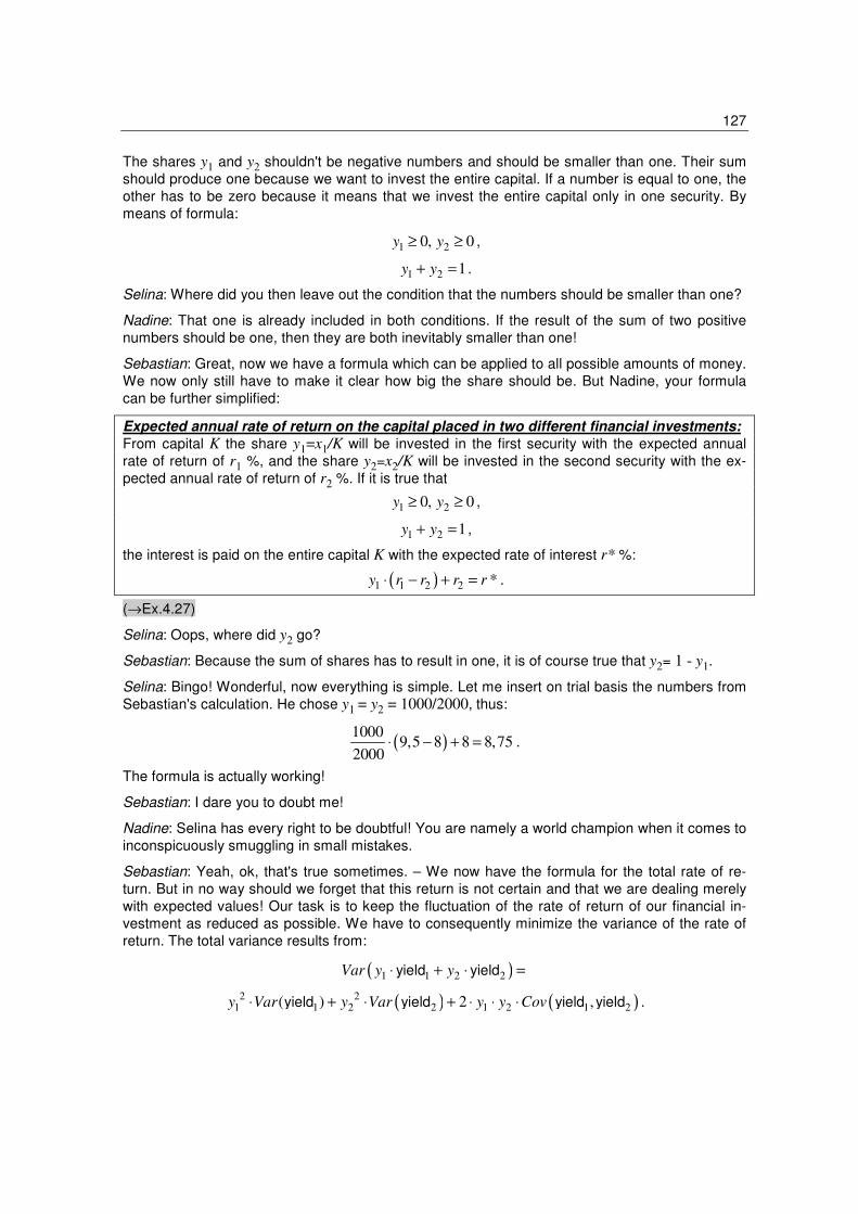
The formula is actually working!

Sebastian: I dare you to doubt me!

Nadine: Selina has every right to be doubtful! You are namely a world champion when it comes to

inconspicuously smuggling in small mistakes.

Sebastian: Yeah, ok, that's true sometimes. – We now have the formula for the total rate of re-

turn. But in no way should we forget that this return is not certain and that we are dealing merely

with expected values! Our task is to keep the fluctuation of the rate of return of our financial in-

vestment as reduced as possible. We have to consequently minimize the variance of the rate of

return. The total variance results from:

( )1 1 2 2yield yieldVar y y⋅ + ⋅ =

( ) ( )2 21 1 2 2 1 2 1 2( ) 2 ,yield yield yield yieldy Var y Var y y Cov⋅ + ⋅ + ⋅ ⋅ ⋅ .

128

To simplify matters let's assume that both rates of return have nothing to do with one another,

that the covariance is thus equal to zero. If y1 represents the share of money in Windig and y2 the

share in Naturstromer, then our minimizing task goes as follows:

2 2

1 2min 0,06 0,04y y⋅ + ⋅ .

(→Ex.4.28)

Selina: Mmh, the squares in the objective function are disagreeable. If only everything were nice

and linear, I could immediately solve the problem. That would be simple minimizing under side

conditions (see Chapter 1). Now the problem looks like this:

2 2

1 2min 0,06 0,04y y⋅ + ⋅

1 2udN 0, 0y y≥ ≥

1 2 1y y+ =

( )1 9,5 8 8 9y ⋅ − + ≥ .

Sebastian: It's not so bad. y2 results from y1,because the result of both should be one. y2 conse-

quently drops out. This is now really simple!

Nadine: You're the only one who thinks that! I myself don't see the solution happening at first go.

It's best we write down the final optimization problem properly without y2:

( )22

1 1min 0,06 1 0,04y y⋅ + − ⋅

1udN 0y ≥

1 1y ≤

( )1 9,5 8 8 9y ⋅ − + ≥ .

Oliver: Nadine and Selina, you're right. The problem is still complex. How about a drawing at this

point?

Chart 4.7 Rate of return - different distribution of capital

The thick line which passes through 9 % indicates the minimal return. The straight line which

starts at (0 , 8 %) indicates how high the return of our total capital is if we invest the share y1 in

company stocks of the Windig Company and the rest of the money in the stocks of Naturstromer

Inc. The minimal return is reached from the intercept point with the 9%-line. From this point starts

the admissible area for y1, which I marked thick on the lower axis. The admissible area ends at y1

= 1.

usc

usc

Rate

of re

turn

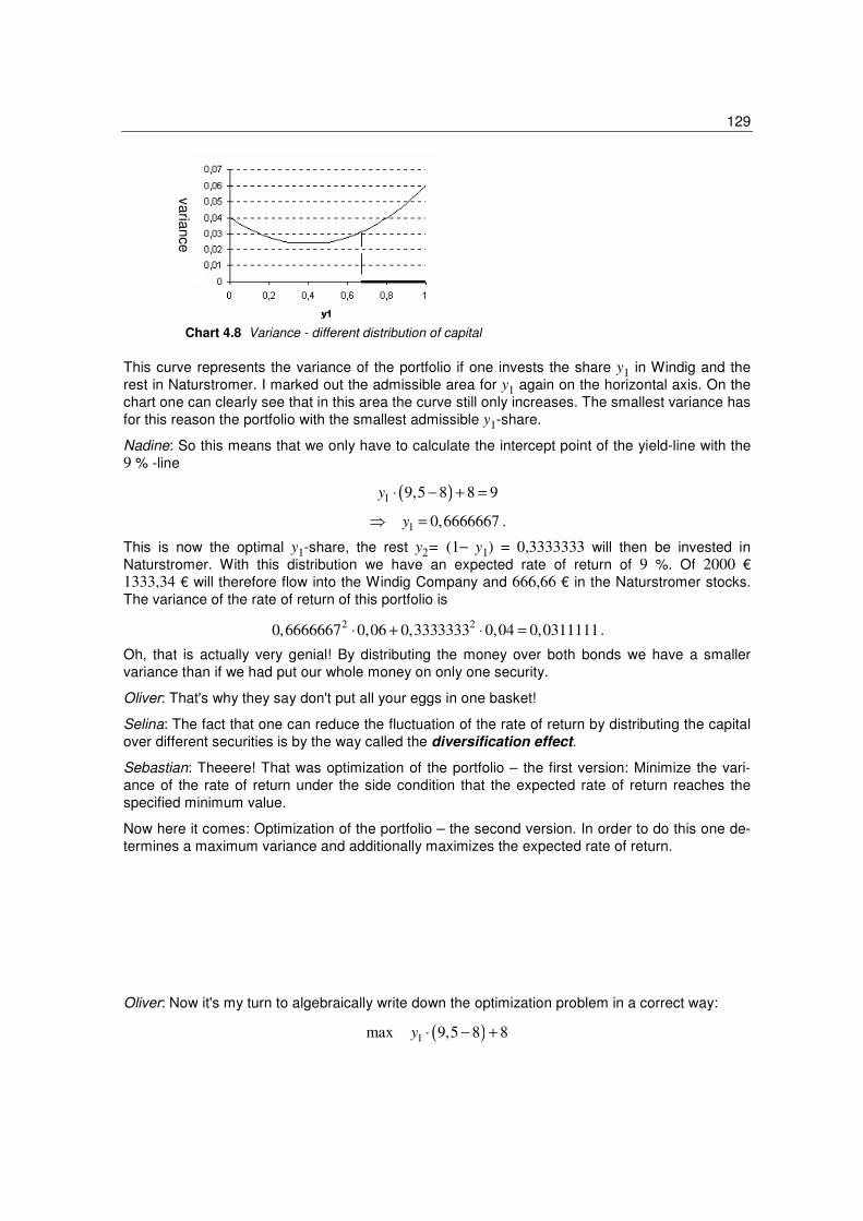
129

Chart 4.8 Variance - different distribution of capital

This curve represents the variance of the portfolio if one invests the share y1 in Windig and the

rest in Naturstromer. I marked out the admissible area for y1 again on the horizontal axis. On the

chart one can clearly see that in this area the curve still only increases. The smallest variance has

for this reason the portfolio with the smallest admissible y1-share.

Nadine: So this means that we only have to calculate the intercept point of the yield-line with the

9 % -line

( )1 9,5 8 8 9y ⋅ − + =

1 0,6666667y⇒ = .

This is now the optimal y1-share, the rest y2= (1− y1) = 0,3333333 will then be invested in

Naturstromer. With this distribution we have an expected rate of return of 9 %. Of 2000 €

1333,34 € will therefore flow into the Windig Company and 666,66 € in the Naturstromer stocks.

The variance of the rate of return of this portfolio is

2 2

0,6666667 0,06 0,3333333 0,04 0,0311111⋅ + ⋅ = .

Oh, that is actually very genial! By distributing the money over both bonds we have a smaller

variance than if we had put our whole money on only one security.

Oliver: That's why they say don't put all your eggs in one basket!

Selina: The fact that one can reduce the fluctuation of the rate of return by distributing the capital

over different securities is by the way called the diversification effect.

Sebastian: Theeere! That was optimization of the portfolio – the first version: Minimize the vari-

ance of the rate of return under the side condition that the expected rate of return reaches the

specified minimum value.

Now here it comes: Optimization of the portfolio – the second version. In order to do this one de-

termines a maximum variance and additionally maximizes the expected rate of return.

Oliver: Now it's my turn to algebraically write down the optimization problem in a correct way:

( )1max 9,5 8 8y ⋅ − +

varia

nce

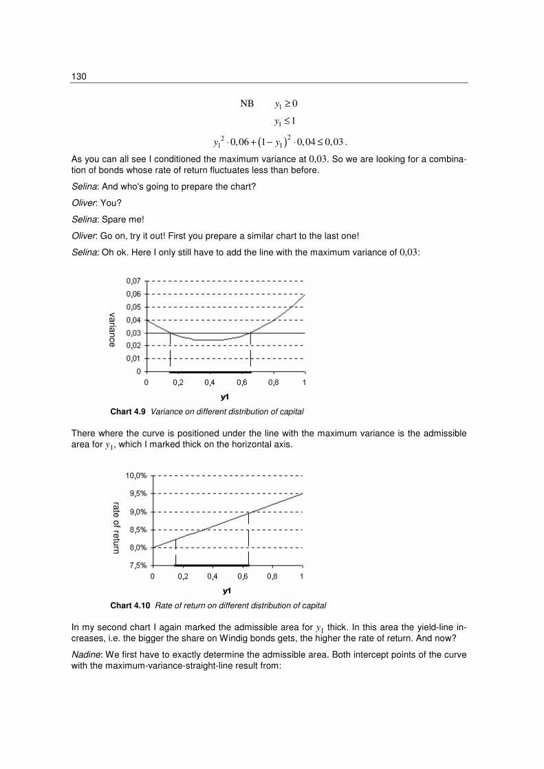
130

1NB 0y ≥

1 1y ≤

( )22

1 10,06 1 0,04 0,03y y⋅ + − ⋅ ≤ .

As you can all see I conditioned the maximum variance at 0,03. So we are looking for a combina-

tion of bonds whose rate of return fluctuates less than before.

Selina: And who's going to prepare the chart?

Oliver: You?

Selina: Spare me!

Oliver: Go on, try it out! First you prepare a similar chart to the last one!

Selina: Oh ok. Here I only still have to add the line with the maximum variance of 0,03:

Chart 4.9 Variance on different distribution of capital

There where the curve is positioned under the line with the maximum variance is the admissible

area for y1, which I marked thick on the horizontal axis.

Chart 4.10 Rate of return on different distribution of capital

In my second chart I again marked the admissible area for y1 thick. In this area the yield-line in-

creases, i.e. the bigger the share on Windig bonds gets, the higher the rate of return. And now?

Nadine: We first have to exactly determine the admissible area. Both intercept points of the curve

with the maximum-variance-straight-line result from:

varia

nce

rate

of re

turn

131

( )22

1 10,06 1 0,04 0,03y y⋅ + − ⋅ =

1 10,15505, 0,64495y y⇒ = = .

Because the yield-straight-line increases in this area, the biggest admissible value also has the

highest expected rate of return. The biggest admissible share for y1 is 0,64495. We have to invest

from the 2000 € initial capital the amount of 1289,90 € in Windig and the rest of 710,10 € in

Naturstromer. The expected rate of return is maximal in case of such distribution. It amounts to:

( )0,64495 9,5 8 8 8,967425⋅ − + = .

Oliver: So, a rate of return of 8,967 %, not bad at all!

Sebastian: Now we have already discovered some interesting investment opportunities. However

we should once again talk to the director and ask him what he means by "optimal", which maxi-

mum variance he wants to have for his financial investment or whether he insists on a minimum

rate of return.

The director barely finished his tea break when he was seized by the Clever Consulting Team

which explained him the mean-variance-principle in detail. And while the director listens carefully,

some new ideas occur to him...

Discussion 6

Why is it not possible to maximize the expected rate of return of the portfolio and at the same

time minimize variance?

Exercises

Ex.4.27 Calculate the expected return on the capital of 2000 € if the amount of x1€ is invested in

shares of the Windig Company and the rest in stocks of Naturstromer Inc.!

a) x1 = 1800 b) x1 = 700 c) x1= 1500

d) x1 = 1100 e) x1 = 900 f ) x1= 2000

Ex.4.28 Calculate the variance of the rate of return if in case of a capital of 2000 € the amount of

x1€ is invested in stocks of the Windig Company and the rest in stocks of Naturstromer Inc.!

a) x1 = 1800 b) x1 = 700 c) x1= 1500

d) x1 = 1100 e) x1 = 900 f ) x1= 2000

Ex.4.29 Set and solve the opitmization problem using the data from the discussion,

a) if the expected rate of return should amount to at least 8,8 %!

b) if the expected rate of return should amount to at least 8,3 %! (Clue: One has to carry out a

function analysis!)

c) if the variance of the rate of return should amount to 0,035 at most!

d) if the variance of the rate of return should amount to 0,05 at most!

4.8 Basic principles of mathematics: The mean-variance-approach

In this section our aim is to introduce the mean-variance-approach for determining optimal in-

vestment strategies. Before we start dealing with theory in detail, we want to firstly point out that

certain criteria for determining the best investment strategy, which may seem absolutely natural,

132

are not practical, and are indeed very problematic. These considerations can be considered in-

teractively in class.

Consideration: What is in effect an „optimal investment strategy“?

The solution to the problem

„Determine the strategy by means of which I can become as rich as possible!“

is for an investor an obvious goal, however certainly no reasonably posed task. The strategy by

means of which one can from available original assets generate the greatest final capital possible

can namely be determined only if already at the beginning, meaning at the point at which the

decision on the pursued strategy is made, the complete price developing of all securities were

established. Consequently one could solve the above-mentioned problem only if one had the

ability to see into the future.

Due to the fact that stock prices are not (exactly) easily predicted, we cannot determine any such

strategy by means of which we could always – independently of the future development of the

stock prices – obtain the biggest closing capital possible. If we set up a stochastic model, i.e. a

model with chance components, for the development of the stock prices, we can only expect to

maximize an appropriate average criterion on all possible future scenarios. For this reason as a

result we have the next self-evident verbalization of the portfolio-problem:

„Determine the strategy which maximizes the expected value of the final capital

E(X(T))!“

This problem can be solved by means of given stochastic model for the securities without the

knowledge on the future as well. The problem which appears in this case has the form of the so-

lution itself. The optimal strategy for the above problem namely consists in investing everything in

a stock with the highest expected rate of return. (The reason for that is the linearity of the ex-

pected value.) However this is a risky strategy through which the final capital can be subjected to

great fluctuation. Already at first sight one will be hardly able to resist the impression that the de-

cision in that case was made based on the maximizing of chance and with complete disregard of

risk. As a result we therefore have the following problem:

„Find a formulation (and solution!) of the portfolio-problem in which risk as well as profit

are appropriately taken into consideration!“ The first systematic approach to the modelling and solution of this problem, the mean-variance-

approach by H. Markowitz (1952), can be seen as the beginning of the modern portfolio-theory.

Its meaning for theory and practice was additionally emphasized by the fact that in 1990 Marko-

witz was awarded a Nobel Prize for economic science. The starting point for Markowitz's ap-

proach is the above-mentioned problem, meaning that the pure maximizing of the expected final

capital E(X(T)) leads to the complete capital being invested in one single stock. In doing so one

ceases to pay attention to the fact that the fluctuation of the final capital around this expected

value can be very strong. In order to constrict this fluctuation, Markowitz introduced the side con-

dition that the variance of the final capital, Var(X(T)), should be inside a predetermined bound.

Herewith should be made clear that the essentially achieved final capital will not be too remote

from the (hoped for) expected value of the final capital. As an optimal investment strategy

Markowitz identified a strategy which under compliance with this side condition on the variance

possesses the maximum expected value E(X(T)). In the following we will firstly deal with the

cases in which we have a choice of two or three bonds and at the end of the section we will ap-

proach a generic case.

a) The mean-variance-approach in case of two bonds

We will observe the situation of an investor who possesses the initial assets of x and wants to

invest them in two different bonds whose current market price is determined at p1 and p2. Since

133

we want to invest our money up to the point in time T, we are interested in the rate of return

(meaning the relative market price changes) of the securities

( )i i

i

i

P T pR

p

−= , i = 1,2,

in a time frame [0,T] of the observed investment problem, whereby Pi(T) is the presently un-

known stock price of i. stock in a time frame T. We will assume that the expected values, the

variance and covariance of the rates of return are determined, i.e. we know

( ) ( ) ( ) ( ) ( )1 1 2 2 11 1 22 2 12 1 2, , , , ,E R E R Var R Var R Cov R Rµ µ σ σ σ= = = = = .

In order to observe only economically sensible cases, we want to exclude the condition under

which both rates of return have a correlation of +1 or -1. Otherwise this would mean that one rate

of return completely depends on the other. We should now look for a security combination in case

of which we can with great certainty reach an acceptable rate of return of the total capital.

We will distribute our capital x within a time frame t = 0 in both percentage shares π1 and π2,

whereupon πi describes the share in total capital which will be invested in the i.stock. In doing so

the conditions

1 2 1 20, 0, 1π π π π≥ ≥ = +

should be true because on the one hand no negative number of stocks should be kept and on the

other the sum of the percentage shares has to result in one. Such a pair (π1,π2) will be desig-

nated as portfolio. If now Xπ(T) signifies the final capital when using the portfolio π = (π1,π2) as a

result we get the belonging portfolio rate of return as

( )X T x

Rx

ππ −

=

and at the same time as a weighted sum of the individual stock profit, for it is true that

1 1 2 2R R Rπ π π= + .

Consequently we obtain the expected value and the variance of the portfolio rate of return as

( ) ( ) ( )1 1 2 2 1 1 2 2E R E R E Rπ π π π µ π µ= + = + ,

( ) ( ) 2 21 1 2 2 1 11 2 22 1 2 122Var R Var R R

π π π π σ π σ π π σ= + = + + .

The above demand on an acceptable rate of return which should be reached with the highest

certainty possible can be interpreted as a problem of minimizing variance of the portfolio rate of

return under the side condition that the expected value of the portfolio rate of return should be at

least K. This problem is a type of the mean-variance-approach by Markowitz and we will solve it

presently. Formally the optmization problem is posed as follows:

(VM) ( )

1 2

2 21 11 1 2 12 2 22

,

1 2 1 2 1 1 2 2

min 2

udN 0, 0, 1 , K

π ππ σ π π σ π σ

π π π π µ π µ π

+ +

≥ ≥ = + + ≥

,

in which case we take on µ1≠ µ2 to simplify matters. If one now cancels the constraint 1= π1+π2

after π2 and inserts this term in the place of π2 into the objective function of the optimization prob-

lem and to simplify matters assumes that

1 2µ µ>

is true (one should not always accept that, because the other way round one can rename the

"first stock" into the "second stock"). In this way one gets the equivalent problem:

usc

134

(VM*)

( ) ( )( )1

211 12 22 1 12 22 1 22

*21 1

1 2

min 2 2

0 1, :K

udN K

πσ σ σ π σ σ π σ

µπ π

µ µ

− + + − +

−≤ ≤ ≥ =

−

.

In order for this problem to contain a solution as well, we will presume that the demand for a

minimum expected value for the rate of return is accomplishable, which is assured in the above

formulation (VM*) through the assumption that

*

1K ≤

We therefore obtain as the admissible area for π1 the interval [max(0 ,K*),1].

In order to solve (VM*) one has to minimize a quadratic function in π1 over a closed interval.

Since |ρ(X,Y)|<1 is true, it follows σ11− 2σ12 + σ22 >0 , i.e. the function which is to be minimized

in (VE*) is an open parabola in π1 with a definite minimum at

22 121

11 12 22

ˆ2

σ σπ

σ σ σ

−=

− +.

Case 1: 22 12 0σ σ− ≤ , thus 1ˆ 0π ≤

In this case the function which is to be minimized is smaller the smaller π1 gets. Consequently we

get the optimal value for π1 as the smallest admissible value with

( )( )1 min max 0, * ,0opt

Kπ = .

Chart 4.11 Case 1: 1

ˆ 0π <

The optimal value of π2 results from

2 11opt optπ π= − .

Case 2: ( )22 12 1ˆ0 thus 0σ σ π− > >

Depending on the circumstance of the minimum 1ˆ1 0π> > (Case 2a) or 1

ˆ 1π ≥ (Case 2b) as a

result we get two possible charts:

usc

135

Chart 4.12 Case 2a: 1

ˆ0 1π< < Chart 4.13 Case 2b: 1ˆ 1π >

In the left picture the absolute minimum lies in the interior of the interval [0,1]. In the right picture

the function to be minimized gets smaller the bigger π1 is. Depending on the shape of the admis-

sible area (i.e. the dependency of the value of K*) from both pictures we obtain the optimal value

for π1 as

1 1

11

1

ˆ ˆ, * 1

ˆ1, * 1

ˆ*, *

opt

if K

if K

K if K

π π

π π

π

≤ ≤

= ≤ ≤ ≤

and the optimal value for π2 through

2 11opt optπ π= − .

We will summarize everything in form of an algorithm (under the assumption µ1>µ2) :

Algorithm: Mean-variance-problem for two securities (formulation (VM))

1. Calculate by means of the given data 2

1 2

*:K

Kµ

µ µ

−=

−. The problem only has a solution if K*≤1.

2. Draw the function ( ) ( ) ( )21 11 22 12 1 12 22 1 222 2f π σ σ σ π σ σ π σ= + − + − +

over the admissible

area ( )*max 0, ,1K

for π1.

136

3. Determine, according to the shape of ( )1f π , over ( )max 0, * ,1K the minimum and obtain

1

* if * 0

0 if * 0

opt K K

Kπ

>=

≤ in case 22 12 0σ σ− ≤ ,

*1 1

*11

* *1

ˆ ˆ, 1

ˆ1, 1

ˆ,

opt

if K

if K

K if K

π π

π π

π

≤ ≤

= ≤ ≤

≤

in case 22 12 0σ σ− > .

4. Calculate the optimal value for π2 with 2 11opt optπ π= − .

Note: In case µ1= µ2 one immediately recognizes that the minimum rate of return demand

1 1 2 2 Kµ π µ π+ ≥

is accomplishable if and only if µ1 ≥ K is true. If this is true, the whole interval [0, 1] is admissible

for π1. We can then determine the optimal pair (π1opt, π2

opt) by means of the above algorithm and

K*=0. Otherwise there is no pair (π1, π2) which fulfils the minimum rate of return demand, i.e. the

admissible area is empty.

Discussion 7:

At this point we can discuss the optimization problem. Is it really the implementation of the de-

mand on a "minimum rate of return with the highest certainty possible"? Are there still other rea-

sonable formulations for this problem? Which other optimization opportunities are available?

(→Ex.4.30)

Note

If the second security in the above derivation is a risk-free investment with the rate of return µ2, it

is true that σ22=σ12=0. One consequently needs no covariance and obtains

( ) 1 1 2 2E Rπ π µ π µ= + ,

( ) ( ) ( ) 2 21 1 2 2 1 1 1 11Var R Var R Var R

π π π µ π π σ= + = = .

This thus results through µ1 >µ2 in the problem

(VM*) 1

21 11

*1 1

min

udN 0 1, K

ππ σ

π π≤ ≤ ≥

,

Due to σ11>0 this problem has (under the assumption K*≤1) evidently the solution

( )*1 max 0,opt

Kπ = , ( )*2 1 max 0,opt

Kπ = − ,

because one has to in Case 1 count on σ22−σ12 ≤ 0.

usc

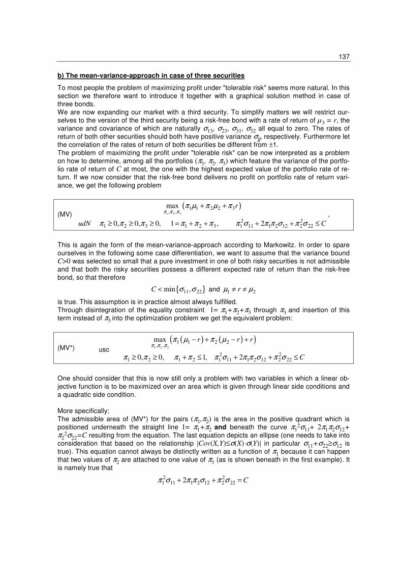
137

b) The mean-variance-approach in case of three securities

To most people the problem of maximizing profit under "tolerable risk" seems more natural. In this

section we therefore want to introduce it together with a graphical solution method in case of

three bonds.

We are now expanding our market with a third security. To simplify matters we will restrict our-

selves to the version of the third security being a risk-free bond with a rate of return of µ3 = r, the

variance and covariance of which are naturally σ13, σ23, σ31, σ32 all equal to zero. The rates of

return of both other securities should both have positive variance σjj, respectively. Furthermore let

the correlation of the rates of return of both securities be different from ±1.

The problem of maximizing the profit under "tolerable risk" can be now interpreted as a problem

on how to determine, among all the portfolios (π1, π2, π3) which feature the variance of the portfo-

lio rate of return of C at most, the one with the highest expected value of the portfolio rate of re-

turn. If we now consider that the risk-free bond delivers no profit on portfolio rate of return vari-

ance, we get the following problem

(MV)

( )1 2 3

1 1 2 2 3, ,

2 21 2 3 1 2 3 1 11 1 2 12 2 22

max

0, 0, 0, 1 , 2

r

udN C

π π ππ µ π µ π

π π π π π π π σ π π σ π σ

+ +

≥ ≥ ≥ = + + + + ≤

,

This is again the form of the mean-variance-approach according to Markowitz. In order to spare

ourselves in the following some case differentiation, we want to assume that the variance bound

C>0 was selected so small that a pure investment in one of both risky securities is not admissible

and that both the risky securities possess a different expected rate of return than the risk-free

bond, so that therefore

11 22min ,C σ σ< and 1 2rµ µ≠ ≠

is true. This assumption is in practice almost always fulfilled.

Through disintegration of the equality constraint 1= π1+π2+π3 through π3 and insertion of this

term instead of π3 into the optimization problem we get the equivalent problem:

(MV*) ( ) ( )( )

1 2 3

1 1 2 2, ,

2 21 2 1 2 1 11 1 2 12 2 22

max

0, 0, 1, 2

r r r

udN C

π π ππ µ π µ

π π π π π σ π π σ π σ

− + − +

≥ ≥ + ≤ + + ≤

One should consider that this is now still only a problem with two variables in which a linear ob-

jective function is to be maximized over an area which is given through linear side conditions and

a quadratic side condition.

More specifically:

The admissible area of (MV*) for the pairs (π1,π2) is the area in the positive quadrant which is

positioned underneath the straight line 1= π1+π2 and beneath the curve π12σ11+ 2π1π2σ12+

π22σ22=C resulting from the equation. The last equation depicts an ellipse (one needs to take into

consideration that based on the relationship |Cov(X,Y)≤σ(X)⋅σ(Y)| in particular σ11+σ22≥σ12 is

true). This equation cannot always be distinctly written as a function of π1 because it can happen

that two values of π2 are attached to one value of π1 (as is shown beneath in the first example). It

is namely true that

2 21 11 1 2 12 2 222 Cπ σ π π σ π σ+ + =

usc

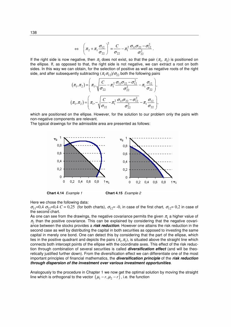
138

⇔

2 2212 11 22 12

2 1 1 222 22 22

Cσ σ σ σπ π π

σ σ σ

−+ = −

.

If the right side is now negative, then π2 does not exist, so that the pair (π1, π2) is positioned on

the ellipse. If, as opposed to that, the right side is not negative, we can extract a root on both

sides. In this way we can obtain, for the selection of positive as well as negative roots of the right

side, and after subsequently subtracting (π1σ12)/σ22 both the following pairs

( )2

2 11 22 12 121 2 1 1 12

22 2222

, ,C σ σ σ σ

π π π π πσ σσ

− = − −

,

( )2

2 11 22 12 121 2 1 1 12

22 2222

, ,C σ σ σ σ

π π π π πσ σσ

− = − − −

,

which are positioned on the ellipse. However, for the solution to our problem only the pairs with

non-negative components are relevant.

The typical drawings for the admissible area are presented as follows:

Chart 4.14 Example 1 Chart 4.15 Example 2

Here we chose the following data:

σ11=0,4 σ22=0,4 C = 0,25 (for both charts), σ12= -0, in case of the first chart, σ12= 0,2 in case of

the second chart.

As one can see from the drawings, the negative covariance permits the given π1 a higher value of

π2 than the positive covariance. This can be explained by considering that the negative covari-

ance between the stocks provides a risk reduction. However one attains the risk reduction in the

second case as well by distributing the capital in both securities as opposed to investing the same

capital in merely one bond. One can detect this by considering that the part of the ellipse, which

lies in the positive quadrant and depicts the pairs (π1,π2), is situated above the straight line which

connects both intercept points of the ellipse with the coordinate axes. This effect of the risk reduc-

tion through combination of several securities is called diversification effect (and will be theo-

retically justified further down). From the diversification effect we can differentiate one of the most

important principles of financial mathematics, the diversification principle of the risk reduction

through dispersion of the investment over various investment opportunities.

Analogously to the procedure in Chapter 1 we now get the optimal solution by moving the straight

line which is orthogonal to the vector ( )1 2,r rµ µ− − , i.e. the function

139

( ) 1

2

rg x x

r

µ

µ

−= −

−,

to the boundary of the admissible area in the direction of the vector ( )1 2,r rµ µ− − . The intersec-

tion point of straight lines and the admissible area constructed in such a way represents the opti-

mal pair ( )1 2,opt optπ π . Depending on the shape of the admissible area one obtains the intersec-

tion point in two manners:

Case 1: There is an intersection point of the ellipse π12σ11+ 2π1π2σ12+ π2

2σ22=C and the straight

line 1= π1+π2.

Here we obtain, by inserting the linear equation into the ellipse equation, meaning by choosing π2 = 1− π1 in the ellipse equation, the quadratic equation

2 12 22 221 1

22 11 12 22 11 12

2 02 2

Cσ σ σπ π

σ σ σ σ σ σ

− −+ + =

+ − + −,

which in this case has two solutions. The solution which results in 1optπ is the component π1 of the

point through which also the straight line, which was shifted to the boundary of the admissible

area, goes, and which is orthogonal to the vector (µ1− r,µ2− r). Furthermore one gets

2 11opt optπ π= − , 3 0

optπ = .

Case 2: There is no intersection point of the ellipse π12σ11+ 2π1π2σ12+ π2

2σ22=C and the

straight line 1= π1+π2.

In this case one obtains the optimal pair (π1opt,π2

opt) as a point in which the shifted straight line

( ) 1

2

b

rg x x b

r

µ

µ

−= − +

−

is a tangent on the ellipse π12σ11+ 2π1π2σ12+ π2

2σ22=C. One therefore does not only have to

determine π1 but also b. In order to achieve that, one inserts the linear equation in the ellipse

equation, i.e. one inserts

12 1 1

2

:r

b a br

µπ π π

µ

−= − + = +

−

and gets the following quadratic equation:

22 12 22 22

1 1 2 211 22 12 11 22 12

2 02 2

b ab b C

a a a a

σ σ σπ π

σ σ σ σ σ σ

+ −+ + =

+ + + +.

This equation contains the still unknown value b. In order to determine this value we will now

apply the fact that this equation has a double null due to the fact that the straight line gb(x) is

merely a tangent to the ellipse. We thus know that the following equation has to be true

for this value b

( )2

22 212 22 22

11 22 122 211 22 12 11 22 12

2 02 2

a b Cb a a

a a a a

σ σ σσ σ σ

σ σ σ σ σ σ

+ −− + + = + + + +

.

Only in case of dependency of the form on gb(x) („decreasing or increasing“) do we choose the

appropriate solution b to this equation:

140

( )

( )

211 12 22

211 22 12

211 12 22

211 22 12

2, 0

2, 0

C a afalls a

b

C a afalls a

σ σ σ

σ σ σ

σ σ σ

σ σ σ

+ ++ > −

= + +− < −

.

Following this path one obtains all the components of the optimal portfolio as

22 121 2

11 22 122

opt ab

a a

σ σπ

σ σ σ

−=

+ +, 1

2 1

2

opt optrb

r

µπ π

µ

−= − +

−, 3 1 21

opt opt optπ π π= − − .

Again we will write everything down in form of an algorithm:

Algorithm: Mean-variance-problem for three securities (in which one is a risk-free financial in-

vestment), formulation (MV)

1. Draw the admissible area

2 21 2 1 2 1 11 1 2 12 2 220, 0, 1, 2 Cπ π π π π σ π π σ π σ≥ ≥ + ≤ + + ≤

provided by the side conditions, for pairs (π1,π2).

2. Shift the straight line which is orthogonal to the vector (µ1 −r, µ2 −r) to the boundary of the

admissible area in the direction of the vector (µ1 −r, µ2 −r).

3. Determine the optimal pair (π1opt, π2

opt) by forming the intersection point according to both

above-mentioned cases 1 and 2.

4. Acquire the optimal value for π3 as 3 1 21opt opt optπ π π= − − .

Discussion 8:

How can one expand the above method for solving (MV) to the case with three risky securities?

Which problems arise if one wants to transfer the solution method for (MV) to the case of those

three securities?

(→Ex.4.31)

c) The mean-variance-approach in generic mode

We will now observe a one-period-model with d stocks whose current prices pi, i =1, ..., d, are

announced. Their prices are given in the final period T of the observed investment problem, Pi(T),

by modelling their rate of return

( )i i

i

i

P T pR

p

−=

We will furthermore assume that the expected values, variance and covariance of the rate of re-

turn are familiar:

( ) ( ) ( ), , , , , 1,...,i i ii i ij i jµ E R Var R σ Cov R R i j dσ= = = = .

Variance and covariance are the components of the so-called covariance matrix σ:

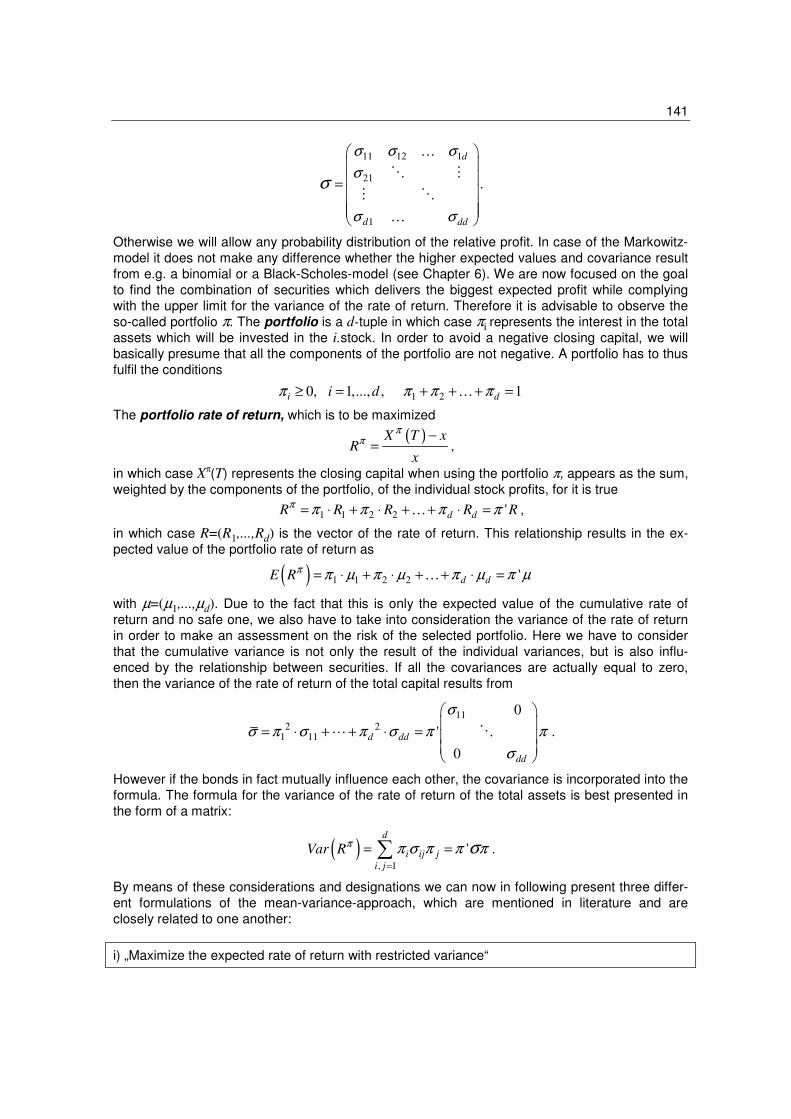
141

11 12 1

21

1

d

d dd

σ σ σ

σ

σ σ

σ

=

…

⋱ ⋮

⋮ ⋱

…

.

Otherwise we will allow any probability distribution of the relative profit. In case of the Markowitz-

model it does not make any difference whether the higher expected values and covariance result

from e.g. a binomial or a Black-Scholes-model (see Chapter 6). We are now focused on the goal

to find the combination of securities which delivers the biggest expected profit while complying

with the upper limit for the variance of the rate of return. Therefore it is advisable to observe the

so-called portfolio π. The portfolio is a d-tuple in which case πi represents the interest in the total

assets which will be invested in the i.stock. In order to avoid a negative closing capital, we will

basically presume that all the components of the portfolio are not negative. A portfolio has to thus

fulfil the conditions

1 20, 1,..., , 1i di dπ π π π≥ = + + + =…

The portfolio rate of return, which is to be maximized

( )X T xR

x

ππ −

= ,

in which case Xπ(T) represents the closing capital when using the portfolio π, appears as the sum,

weighted by the components of the portfolio, of the individual stock profits, for it is true

1 1 2 2 'd dR R R R Rπ π π π π= ⋅ + ⋅ + + ⋅ =… ,

in which case R=(R1,...,Rd) is the vector of the rate of return. This relationship results in the ex-

pected value of the portfolio rate of return as

( ) 1 1 2 2 'd dE Rπ π µ π µ π µ π µ= ⋅ + ⋅ + + ⋅ =…

with µ=(µ1,...,µd). Due to the fact that this is only the expected value of the cumulative rate of

return and no safe one, we also have to take into consideration the variance of the rate of return

in order to make an assessment on the risk of the selected portfolio. Here we have to consider

that the cumulative variance is not only the result of the individual variances, but is also influ-

enced by the relationship between securities. If all the covariances are actually equal to zero,

then the variance of the rate of return of the total capital results from

11

2 21 11

0

'

0

d dd

dd

σ

σ π σ π σ π π

σ

= ⋅ + + ⋅ =

⋯ ⋱ .

However if the bonds in fact mutually influence each other, the covariance is incorporated into the

formula. The formula for the variance of the rate of return of the total assets is best presented in

the form of a matrix:

( ), 1

'd

i ij j

i j

Var Rπ π σ π π πσ

=

= =∑ .

By means of these considerations and designations we can now in following present three differ-

ent formulations of the mean-variance-approach, which are mentioned in literature and are

closely related to one another:

i) „Maximize the expected rate of return with restricted variance“

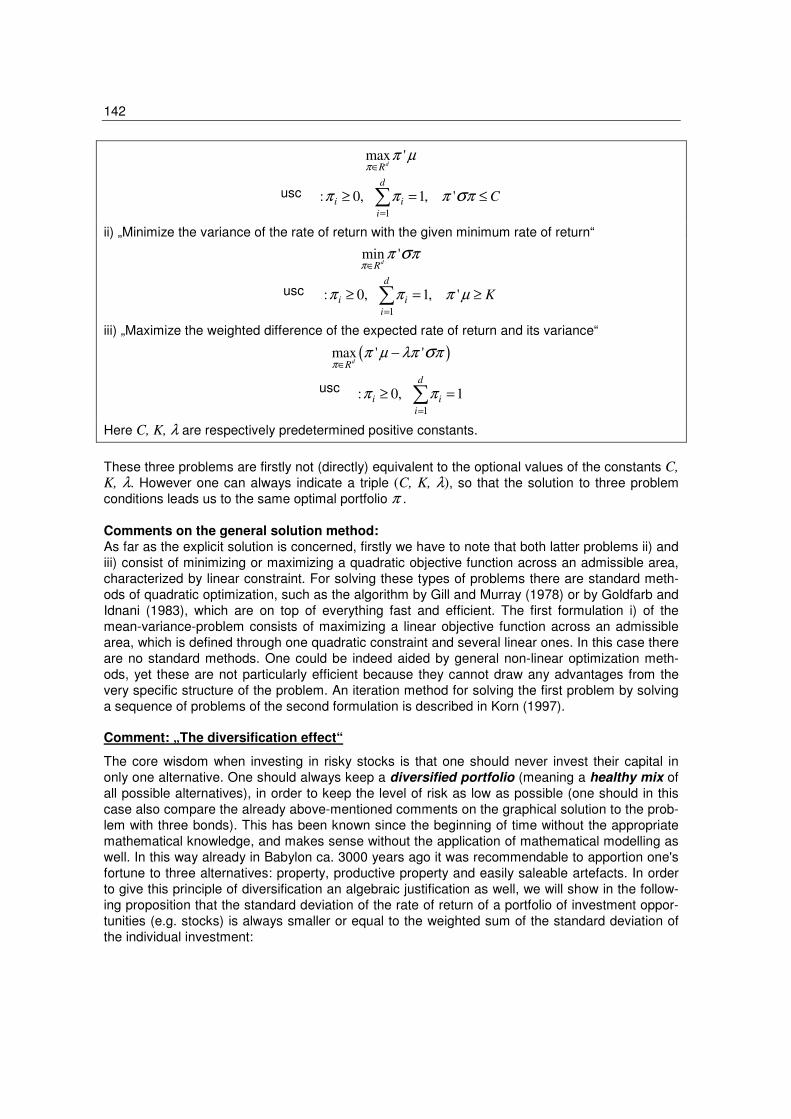
142

1

max '

. . .: 0, 1, '

dR

d

i i

i

u d N C

ππ µ

π π π πσ

∈

=

≥ = ≤∑

ii) „Minimize the variance of the rate of return with the given minimum rate of return“

1

min '

. . .: 0, 1, '

dR

d

i i

i

u d N K

ππ π

π π π µ

σ∈

=

≥ = ≥∑

iii) „Maximize the weighted difference of the expected rate of return and its variance“

( )

1

max ' '

. . .: 0, 1

dR

d

i i

i

u d N

ππ µ λπ π

π π

σ∈

=

−

≥ =∑

Here C, K, λ are respectively predetermined positive constants.

These three problems are firstly not (directly) equivalent to the optional values of the constants C, K, λ. However one can always indicate a triple (C, K, λ), so that the solution to three problem

conditions leads us to the same optimal portfolio π .

Comments on the general solution method:

As far as the explicit solution is concerned, firstly we have to note that both latter problems ii) and

iii) consist of minimizing or maximizing a quadratic objective function across an admissible area,

characterized by linear constraint. For solving these types of problems there are standard meth-

ods of quadratic optimization, such as the algorithm by Gill and Murray (1978) or by Goldfarb and

Idnani (1983), which are on top of everything fast and efficient. The first formulation i) of the

mean-variance-problem consists of maximizing a linear objective function across an admissible

area, which is defined through one quadratic constraint and several linear ones. In this case there

are no standard methods. One could be indeed aided by general non-linear optimization meth-

ods, yet these are not particularly efficient because they cannot draw any advantages from the

very specific structure of the problem. An iteration method for solving the first problem by solving

a sequence of problems of the second formulation is described in Korn (1997).

Comment: „The diversification effect“

The core wisdom when investing in risky stocks is that one should never invest their capital in

only one alternative. One should always keep a diversified portfolio (meaning a healthy mix of

all possible alternatives), in order to keep the level of risk as low as possible (one should in this

case also compare the already above-mentioned comments on the graphical solution to the prob-

lem with three bonds). This has been known since the beginning of time without the appropriate

mathematical knowledge, and makes sense without the application of mathematical modelling as

well. In this way already in Babylon ca. 3000 years ago it was recommendable to apportion one's

fortune to three alternatives: property, productive property and easily saleable artefacts. In order

to give this principle of diversification an algebraic justification as well, we will show in the follow-

ing proposition that the standard deviation of the rate of return of a portfolio of investment oppor-

tunities (e.g. stocks) is always smaller or equal to the weighted sum of the standard deviation of

the individual investment:

usc

usc

usc

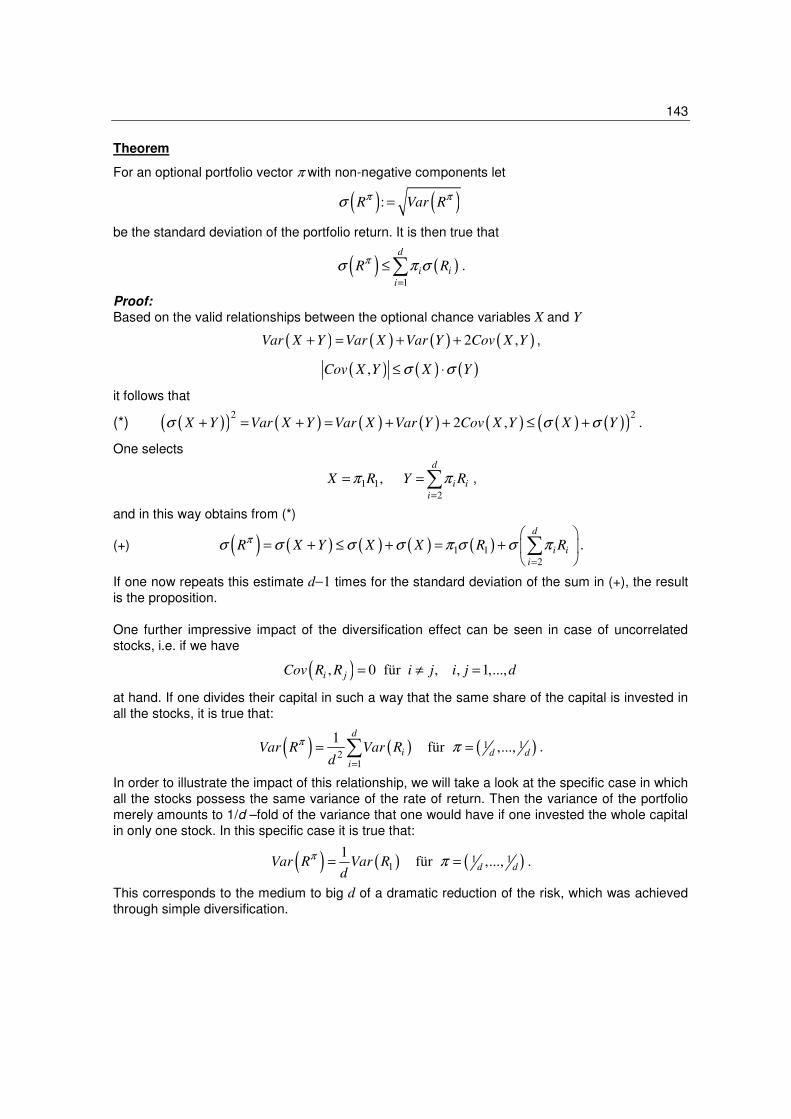
143

Theorem

For an optional portfolio vector π with non-negative components let

( ) ( ):R Var Rπ πσ =

be the standard deviation of the portfolio return. It is then true that

( ) ( )1

d

i i

i

R Rπσ π σ

=

≤∑ .

Proof:

Based on the valid relationships between the optional chance variables X and Y

( ) ( ) ( ) ( )2 ,Var X Y Var X Var Y Cov X Y+ = + + ,

( ) ( ) ( ),Cov X Y X Yσ σ≤ ⋅

it follows that

(*) ( )( ) ( ) ( ) ( ) ( ) ( ) ( )( )2 2

2 ,X Y Var X Y Var X Var Y Cov X Y X Yσ σ σ+ = + = + + ≤ + .

One selects

1 1

2

,d

i i

i

X R Y Rπ π=

= =∑ ,

and in this way obtains from (*)

(+) ( ) ( ) ( ) ( ) ( )1 1

2

d

i i

i

R X Y X X R Rπσ σ σ σ π σ σ π

=

= + ≤ + = +

∑ .

If one now repeats this estimate d−1 times for the standard deviation of the sum in (+), the result

is the proposition.

One further impressive impact of the diversification effect can be seen in case of uncorrelated

stocks, i.e. if we have

( ), 0 für , , 1,...,i jCov R R i j i j d= ≠ =

at hand. If one divides their capital in such a way that the same share of the capital is invested in

all the stocks, it is true that:

( ) ( ) ( )1 12

1

1für ,...,

d

i d d

i

Var R Var Rd

π π=

= =∑ .

In order to illustrate the impact of this relationship, we will take a look at the specific case in which

all the stocks possess the same variance of the rate of return. Then the variance of the portfolio

merely amounts to 1/d –fold of the variance that one would have if one invested the whole capital

in only one stock. In this specific case it is true that:

( ) ( ) ( )1 11

1für ,...,d dVar R Var R

d

π π= = .

This corresponds to the medium to big d of a dramatic reduction of the risk, which was achieved

through simple diversification.

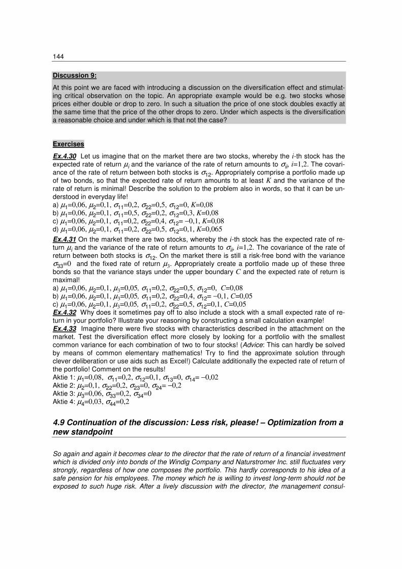
144

Discussion 9:

At this point we are faced with introducing a discussion on the diversification effect and stimulat-

ing critical observation on the topic. An appropriate example would be e.g. two stocks whose

prices either double or drop to zero. In such a situation the price of one stock doubles exactly at

the same time that the price of the other drops to zero. Under which aspects is the diversification

a reasonable choice and under which is that not the case?

Exercises

Ex.4.30 Let us imagine that on the market there are two stocks, whereby the i-th stock has the

expected rate of return µi and the variance of the rate of return amounts to σii, i=1,2. The covari-

ance of the rate of return between both stocks is σ12. Appropriately comprise a portfolio made up

of two bonds, so that the expected rate of return amounts to at least K and the variance of the

rate of return is minimal! Describe the solution to the problem also in words, so that it can be un-

derstood in everyday life!

a) µ1=0,06, µ2=0,1, σ11=0,2, σ22=0,5, σ12=0, K=0,08

b) µ1=0,06, µ2=0,1, σ11=0,5, σ22=0,2, σ12=0,3, K=0,08

c) µ1=0,06, µ2=0,1, σ11=0,2, σ22=0,4, σ12= −0,1, K=0,08

d) µ1=0,06, µ2=0,1, σ11=0,2, σ22=0,5, σ12=0,1, K=0,065

Ex.4.31 On the market there are two stocks, whereby the i-th stock has the expected rate of re-

turn µi and the variance of the rate of return amounts to σii, i=1,2. The covariance of the rate of

return between both stocks is σ12. On the market there is still a risk-free bond with the variance

σ33=0 and the fixed rate of return µ3. Appropriately create a portfolio made up of these three

bonds so that the variance stays under the upper boundary C and the expected rate of return is

maximal!

a) µ1=0,06, µ2=0,1, µ3=0,05, σ11=0,2, σ22=0,5, σ12=0, C=0,08

b) µ1=0,06, µ2=0,1, µ3=0,05, σ11=0,2, σ22=0,4, σ12= −0,1, C=0,05

c) µ1=0,06, µ2=0,1, µ3=0,05, σ11=0,2, σ22=0,5, σ12=0,1, C=0,05

Ex.4.32 Why does it sometimes pay off to also include a stock with a small expected rate of re-

turn in your portfolio? Illustrate your reasoning by constructing a small calculation example!

Ex.4.33 Imagine there were five stocks with characteristics described in the attachment on the

market. Test the diversification effect more closely by looking for a portfolio with the smallest

common variance for each combination of two to four stocks! (Advice: This can hardly be solved

by means of common elementary mathematics! Try to find the approximate solution through

clever deliberation or use aids such as Excel!) Calculate additionally the expected rate of return of

the portfolio! Comment on the results!

Aktie 1: µ1=0,08, σ11=0,2, σ12=0,1, σ13=0, σ14= −0,02

Aktie 2: µ2=0,1, σ22=0,2, σ23=0, σ24= −0,2

Aktie 3: µ3=0,06, σ33=0,2, σ34=0

Aktie 4: µ4=0,03, σ44=0,2

4.9 Continuation of the discussion: Less risk, please! – Optimization from a new standpoint

So again and again it becomes clear to the director that the rate of return of a financial investment

which is divided only into bonds of the Windig Company and Naturstromer Inc. still fluctuates very

strongly, regardless of how one composes the portfolio. This hardly corresponds to his idea of a

safe pension for his employees. The money which he is willing to invest long-term should not be

exposed to such huge risk. After a lively discussion with the director, the management consul-

145

tancy team again meets in the conference room, in which it is in the meantime due to the gloomy

clouds so dark that one would best call it a day.

Nadine: Will somebody turn on that light! What with the storm out there, the electricity doesn't

cost a thing today.

Sebastian: It's storming inside of me now too. Imagine, the director is insisting on the maximal-

variance of 0,001!

Nadine: After it became clear to him what the whole deal with the variance of the rate of return is,

the uncertainty of the financial investment was too big for him. He wants his pension to be also

really safe.

Sebastian: Variance of 0,001 with these securities! Impossible! Look at Oliver's and Selina's

charts (4.7 and 4.8) again! This variance can definitely not be achieved. The smallest variance

possible is approximately at 0,025.

Nadine: Exactly at 0,024!

Sebastian: Yeah ok. If one now solves the last optimization problem for all the variance bounds

C, which are grantable, one gets an optimal expected rate of return for each C. The variance

bound C=0,001 is however not grantable!

Oliver: Sounds yet again like a task for me! So I will now immediately draw up a chart on which

for each admissible variance bound we will enter the expected optimal rate of return:

(→Ex.4.34)

Chart 4.16 Mean-variance-efficient set

Sebastian: The graph of a function obtained in such a way is by the way called mean-variance-

efficient set. Besides in this set all the pairs which represent the solutions to our first problem

formulation of the mean-variance-problem are located. You have to just let the expected value

bound run through all the values in which the demand for the minimum rate of return also repre-

sents a true side condition.

Nadine: And who cares? The variance is still too big for the boss! Back to the main topic. Yeah,

so I suggested to him to invest part of the money in fixed interest bonds anyway. In that case at

the moment there is interest of exactly 5 % per year and this is certain indeed! No fluctuation or

variance! This time he could chum up with the idea of such boring bonds.

Expecte

d ra

te o

f retu

rn

variance

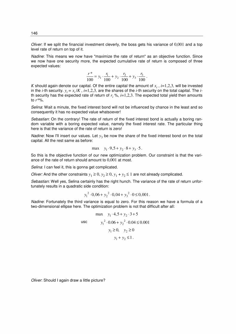
146

Oliver: If we split the financial investment cleverly, the boss gets his variance of 0,001 and a top

level rate of return on top of it.

Nadine: This means we now have "maximize the rate of return" as an objective function. Since

we now have one security more, the expected cumulative rate of return is composed of three

expected values:

31 21 2 3

*

100 100 100 100

rr rry y y= ⋅ + ⋅ + ⋅ .

K should again denote our capital. Of the entire capital the amount of xi , i=1,2,3, will be invested

in the i-th security. yi = xi /K , i=1,2,3, are the shares of the i-th security on the total capital. The i-th security has the expected rate of return of ri %, i=1,2,3. The expected total yield then amounts

to r*%.

Selina: Wait a minute, the fixed interest bond will not be influenced by chance in the least and so

consequently it has no expected value whatsoever!

Sebastian: On the contrary! The rate of return of the fixed interest bond is actually a boring ran-

dom variable with a boring expected value, namely the fixed interest rate. The particular thing

here is that the variance of the rate of return is zero!

Nadine: Now I'll insert our values. Let y3 be now the share of the fixed interest bond on the total

capital. All the rest same as before:

1 2 3max 9,5 8 5y y y⋅ + ⋅ + ⋅ .

So this is the objective function of our new optimization problem. Our constraint is that the vari-

ance of the rate of return should amount to 0,001 at most.

Selina: I can feel it, this is gonna get complicated.

Oliver: And the other constraints y1 ≥ 0, y2 ≥ 0, y1 + y2 ≤ 1 are not already complicated.

Sebastian: Well yes, Selina certainly has the right hunch. The variance of the rate of return unfor-

tunately results in a quadratic side condition:

2 2 2

1 2 30,06 0,04 0 0,001y y y⋅ + ⋅ + ⋅ ≤ .

Nadine: Fortunately the third variance is equal to zero. For this reason we have a formula of a

two-dimensional ellipse here. The optimization problem is not that difficult after all:

1 2max 4,5 3 5y y⋅ + ⋅ +

2 2

1 2udN 0.06 0.04 0.001y y⋅ + ⋅ ≤

1 20, 0y y≥ ≥

1 2 1y y+ ≤ .

Oliver: Should I again draw a little picture?

usc

147

Chart 4.17 Portfolios with variance smaller / equal 0,001

For the variance I drew the following curve:

21

2

0,001 0,06

0,04

yy

− ⋅= .

This is the curve of all the portfolios with the variance of the rate of return equal to 0,001. Portfo-

lios whose variance is smaller than 0,001 are positioned under this curve. The grey area beneath

the curve is thus the admissible area. The side condition y1+y2 ≤ 1 is of no relevance in this case.

The condition that the variance should be small is so strong that y1 and y2 both have to stay very

small and even as a sum not come anywhere near one. This time we have a linear objective func-

tion, and that we can deal with graphically. We will shift the straight line of the objective function

2 1

* 5 4,5

3 3

ry y

−= − ⋅

for different fixed rate of return values r* simply parallel to the upper right:

Chart 4.18 Admissible area with objective function

148

The lower straight line belongs to rate of return of 5,5 %, the upper one to the rate of return of

5,75 %. It looks as if the upper straight line and the curve of the variance were intersecting in

exactly one point. Straight lines with a higher rate of return do not intersect with the admissible

area, because they lie parallel across these straight lines. The rate of return of 5,75 % seems to

be the maximal rate of return which can be achieved by a portfolio with a variance under 0,001.

Now we almost have a solution, but I can't somehow picture all this. I have to create a table with

concrete numbers. (→Ex.4.35)

Nadine: Oliver, I'm not really sure if this whole thing with the maximal rate of return of 5,75 % is that correct. That which we can distinguish in a drawing is still in most cases pretty imprecise. In order to find the exact result you have to find the yield-straight-line which has exactly one inter-cept point with the variance-ellipse of 0,001 in common. For this I will set the yield-straight-line and the variance-ellipse equal:

21

1

0,001 0,06* 5 4,5

3 3 0,04

yry

− ⋅−− ⋅ = .

Selina: Wait a minute, Nadine! You still don't know the optimal r* at all!

Nadine: This is exactly the trick. I have additionally the information that the straight line is allowed

to only touch the ellipse, right? So I can calculate some more in peace and square both sides...

While Oliver is creating his table, Nadine calculating, Selina refreshing her makeup in the ladies'

room, Sebastian unpacks the company Notebook, types fervently and calls out suddenly:

Sebastian: The optimal expected rate of return is 5,75 %.

Nadine: That's what I just calculated too! How did you get to the solution so fast?

Sebastian: Well, it did pay off that our consultancy followed my advice and bought the new opti-

mization-software anyway!

Oliver: Party pooper! This time you could have also calculated it manually!

Sebastian: As soon as you have to observe more bonds and take into consideration perhaps

covariances and other stuff, you won't stand a chance! However, Oliver, words of praise for you,

you really drew accurately!

Nadine: I have the following result:

1 2 30,1, 0,1 , 0,8y y y= = = .

Sebastian, does this coincide with your values?

Sebastian: Yes, I got that too. With this distribution of 2000 € with the determined maximum vari-

ance of 0,001 we would have the best rate of return, namely 5,75 %.

Oliver: But what does, when you get right down to it, the variance of 0,001 for the rate of return of

5,75 % mean?

Nadine: From the variance one can calculate the standard deviance of the rate of return:

( ) 0,001yieldσ = .

In this way you can indicate an approximate area for the rate of return. Casually one could only say that the rate of return of this financial investment after a year is located approximately be-tween

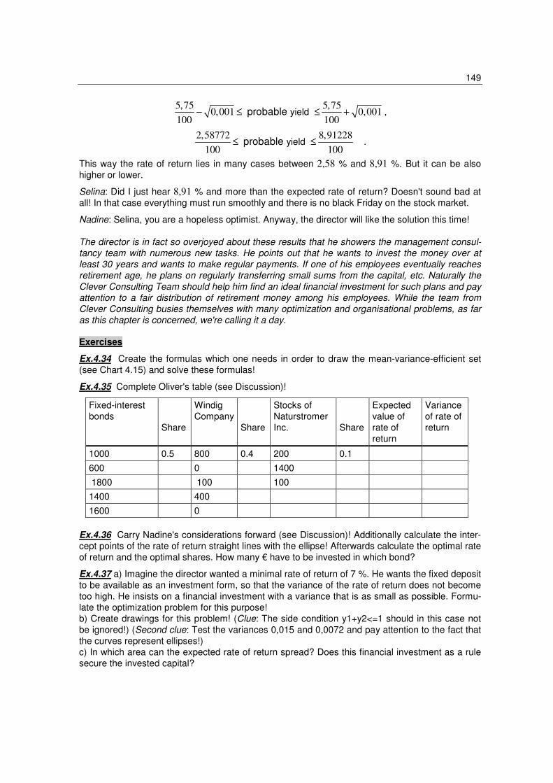
149

5,75 5,75

0,001 0,001100 100

yieldprobable− ≤ ≤ + ,

2,58772 8,91228

100 100

yieldprobable≤ ≤ .

This way the rate of return lies in many cases between 2,58 % and 8,91 %. But it can be also

higher or lower.

Selina: Did I just hear 8,91 % and more than the expected rate of return? Doesn't sound bad at

all! In that case everything must run smoothly and there is no black Friday on the stock market.

Nadine: Selina, you are a hopeless optimist. Anyway, the director will like the solution this time!

The director is in fact so overjoyed about these results that he showers the management consul-

tancy team with numerous new tasks. He points out that he wants to invest the money over at

least 30 years and wants to make regular payments. If one of his employees eventually reaches

retirement age, he plans on regularly transferring small sums from the capital, etc. Naturally the

Clever Consulting Team should help him find an ideal financial investment for such plans and pay

attention to a fair distribution of retirement money among his employees. While the team from

Clever Consulting busies themselves with many optimization and organisational problems, as far

as this chapter is concerned, we're calling it a day.

Exercises

Ex.4.34 Create the formulas which one needs in order to draw the mean-variance-efficient set

(see Chart 4.15) and solve these formulas!

Ex.4.35 Complete Oliver's table (see Discussion)!

Fixed-interest

bonds

Share

Windig

Company

Share

Stocks of

Naturstromer

Inc.

Share

Expected

value of

rate of

return

Variance

of rate of

return

1000 0.5 800 0.4 200 0.1

600 0 1400

1800 100 100

1400 400

1600 0

Ex.4.36 Carry Nadine's considerations forward (see Discussion)! Additionally calculate the inter-

cept points of the rate of return straight lines with the ellipse! Afterwards calculate the optimal rate

of return and the optimal shares. How many € have to be invested in which bond?

Ex.4.37 a) Imagine the director wanted a minimal rate of return of 7 %. He wants the fixed deposit

to be available as an investment form, so that the variance of the rate of return does not become

too high. He insists on a financial investment with a variance that is as small as possible. Formu-

late the optimization problem for this purpose!

b) Create drawings for this problem! (Clue: The side condition y1+y2<=1 should in this case not

be ignored!) (Second clue: Test the variances 0,015 and 0,0072 and pay attention to the fact that

the curves represent ellipses!)

c) In which area can the expected rate of return spread? Does this financial investment as a rule

secure the invested capital?

150

4.10 Summary

In the previous sections we studied how an amount of money can be distributed and invested.

Such a combination of different securities is called a portfolio. If we are familiar with the ex-

pected values and variances of rate of return of individual securities, as well as their covariance,

we can by means of mean-variance-approach determine an optimal portfolio. Depending on

the preference of the investor, we get as a result two different possible conceptual formulations of

the optimization problem:

Optimization problem 1: „Maximize the expected total rate of return of the portfolio“

One sets a variance of the total yield at C at most. Among all the possible portfolios which fulfil

this condition one determines the combination with the highest expected rate of return.

Optimization problem 2: „Minimize the total variance of the portfolio“

One sets an expected total yield of at least K. Among all possible portfolios which fulfill this condi-

tion one determines the combination with the smallest variance of the rate of return.

For this purpose we introduced graphical solution methods for investment cases in two or three

bonds.

4.11 Portfolio-optimization: Critique on the mean-variance-approach and current research aspects

The mean-variance-approach for the purpose of portfolio-optimization is still often applied in prac-

tice today, although it was developed by H. Markowitz as early as 1952. As mentioned before

Markowitz received, along with two other scientists, the Nobel Prize for economic science in the

year 1990. However, this approach is subject to criticism as well.

Accordingly variance is debatable as a measure of risk because a minimization or restriction of

variance, as envisioned in the Markowitz-approach, basically likewise punishes the desired posi-

tive deviations of the portfolio rate of return from its expected value. From this perspective the

variance minimization represents also (at least partially) the chance minimization. There are

therefore many works in literature in which the variance of the portfolio rate of return is replaced

by other risk measures, such as e.g. the Value-at-Risk (a quantile of the rate of return on a speci-

fied level).

The most serious disadvantage of the mean-variance-approach is that its basis is formed by a so-

called one-period-model. In this case we take into consideration merely a single transaction

period (which can by all means describe a big time span). At the beginning of this time period the

investor compiles his portfolio according to the chosen mean-variance-criterion and retains it in

the same form until the end of the period. Regardless of what happens on the stock market in the

meantime, one does not change the portfolio (at least as a model). At the same time the model-

ling of the stock prices in an extremely simplified way takes place. The price trend of a single

stock on the interval [0,T] is determined merely through its expected value and the variance of its

rate of return, as well as covariance of the rate of return with the yield of the other stocks. There

is no modelling of the stock price in the time lapse.

In order to eliminate this disadvantage from such a statistical approach, in the new theory of fi-

nancial mathematics in general and more specifically as part of portfolio-optimization we observe

the so-called more-period-models. In this case the investor is allowed to trade in either more,

finitely many points in time or even continuously in a time lapse. This is accompanied by a more-

period modelling of the stock prices. In this way the practitioners in the field of derivatives trade

151

normally use the continuous time stock price models as for example the Black-Scholes-Model

(see Chapter 6).

In the domain of portfolio optimization within the more-period-models very often the expected

value of the utility from the attained closing capital is maximized. This utility is modelled through

a monotonously increasing, concave function, which on the one hand indicates that the investor

likes more money rather than less, yet on the other hand with an increasing capital he obtains a

smaller profit from each further monetary unit (here we also speak of „decreasing final utility“). By

introducing a utility function we model the fact that the investor is not necessarily concerned with

the absolute utility numbers, but more with the consequences ("the gain") of these earnings.

Aside from that the adopting a concave profit function leads us automatically to the following: in

case of an equal expected value of the closing capital, a risk-free investment strategy is always

going to be favoured to the one fraught with risk. In this way one incorporated the risk-averse

behaviour into the function and does not need a variance bound as a side condition.

The prime example of such a utility function is the natural logarithm. If an investor in a time-

continuous model (e.g. the Black-Scholes-Model) wants to maximize his logarithmic utility, the

optimal solution requires him to trade with his bonds at all times in order to keep the percentage

share of the capital invested in individual bonds constant. However this is for physical reasons

(„no infinite reaction rate“) as well as for financial reasons („continual trade leads to ruin due to

incidental transaction costs“) not possible. Yet it can be shown (see Rogers (2001)) that for ex-

ample a mere weekly adaptation of the relationships to the optimal strategy leads to only insignifi-

cant deviations compared to the utility attained from the optimal time-continuous strategy.

Further current aspects of the research in the field of portfolio-optimization are the consideration

of incidental transaction costs on the market, portfolio-optimization with uncertain market coeffi-

cients, optimization under consolidation of options, determining of optimal strategies under the

risk of an impending crash, decision-making on the optimal investment with specification of high-

est values for ascertained risk measures, optimal investment for securities, etc.

Surely this spectrum is too wide in order to provide even only a to some degree complete over-

view. It should be simply clarified that there are still many current practice-oriented problems in

the field of portfolio-optimization to be solved. More on modern methods of portfolio-optimization

can be found in e.g. Korn and Korn (2001) or in Korn (1997).

4.12 Further exercises

The Excel program Examples1.xls offers the opportunity to play through different scenarios.

Change the entry-data in colored boxes, e.g. the individual rates of return, and try to interpret the

graphics!