Porous Media Flow Module - COMSOL Documentation

INTRODUCTION TO

Porous Media Flow Module

C o n t a c t I n f o r m a t i o nVisit the Contact COMSOL page at www.comsol.com/contact to submit general inquiries or

search for an address and phone number. You can also visit the Worldwide Sales Offices page at

www.comsol.com/contact/offices for address and contact information.

If you need to contact Support, an online request form is located at the COMSOL Access page at

www.comsol.com/support/case. Other useful links include:

• Support Center: www.comsol.com/support

• Product Download: www.comsol.com/product-download

• Product Updates: www.comsol.com/support/updates

• COMSOL Blog: www.comsol.com/blogs

• Discussion Forum: www.comsol.com/forum

• Events: www.comsol.com/events

• COMSOL Video Gallery: www.comsol.com/videos

• Support Knowledge Base: www.comsol.com/support/knowledgebase

Part number: CM024802

I n t r o d u c t i o n t o t h e P o r o u s M e d i a F l o w M o d u l e© 1998–2021 COMSOL

Protected by patents listed on www.comsol.com/patents, or see Help>About COMSOL Multiphysics on the File menu in the COMSOL Desktop for a less detailed lists of U.S. Patents that may apply. Patents pending.

This Documentation and the Programs described herein are furnished under the COMSOL Software License Agreement (www.comsol.com/comsol-license-agreement) and may be used or copied only under the terms of the license agreement.

COMSOL, the COMSOL logo, COMSOL Multiphysics, COMSOL Desktop, COMSOL Compiler, COMSOL Server, and LiveLink are either registered trademarks or trademarks of COMSOL AB. All other trademarks are the property of their respective owners, and COMSOL AB and its subsidiaries and products are not affiliated with, endorsed by, sponsored by, or supported by those trademark owners. For a list of such trademark owners, see www.comsol.com/trademarks.

Version: COMSOL 6.0

http://www.comsol.com/contact/

http://www.comsol.com/contact/offices/

http://www.comsol.com/support/case/

http://www.comsol.com/support/

http://www.comsol.com/product-download/

http://www.comsol.com/support/updates/

http://www.comsol.com/blogs/

http://www.comsol.com/forum/

http://www.comsol.com/events/

http://www.comsol.com/videos/

http://www.comsol.com/support/knowledgebase/

www.comsol.com/patents/

https://www.comsol.com/comsol-license-agreement/

https://www.comsol.com/trademarks/

https://www.comsol.com/trademarks/

Contents

Introduction . . . . . . . . . . . . . . . . . . . . . . . . . . . . . . . . . . . . . . . . . . . 5

Porous Media Flow Module Interfaces . . . . . . . . . . . . . . . . . . . . . 6

Chemical Reaction and Mass Transport. . . . . . . . . . . . . . . . . . . . . . . 7

Fluid Flow. . . . . . . . . . . . . . . . . . . . . . . . . . . . . . . . . . . . . . . . . . . . . . . . 9

Porous Media Flow. . . . . . . . . . . . . . . . . . . . . . . . . . . . . . . . . . . . . . . . 9

Heat Transfer . . . . . . . . . . . . . . . . . . . . . . . . . . . . . . . . . . . . . . . . . . . 11

Structural Mechanics. . . . . . . . . . . . . . . . . . . . . . . . . . . . . . . . . . . . . . 13

Physics Interface Guide by Space Dimension and Study Type . . . 13

Tutorial Model — Packed Bed Latent Heat Storage. . . . . . . . . 18

| 3

4 |

Introduction

Porous media are encountered in many natural and man-made systems. The need for advanced porous media modeling spans many industries and application areas such as processes in fuel cells, drying of pulp and paper, food production, filtration processes, and so on.The Porous Media Flow Module extends the COMSOL Multiphysics modeling environment to the quantitative investigation of mass, momentum and energy transport in porous media. It is designed for researchers, engineers, teachers, and students, and it suits both single-physics and multiphysics modeling. The contents of the Porous Media Flow Module are a set of fundamental building blocks which cover a wide array of physics questions. The physics interfaces it offers work on their own or linked to each other. They can also be coupled to physics interfaces already built into COMSOL Multiphysics, or to new equations you create. The physics interfaces, options, and functionalities in this module are tailored to account for processes in porous media. The Heat Transfer interfaces, for example, include options to automate the calculation of effective thermal properties for multicomponent systems. The fluid flow equations represent a wide range of possibilities. Included are Richards’ equation, which describes nonlinear flow in variably saturated porous media. The options for saturated porous media include Darcy’s law for slow flow and the Brinkman equations where shear is non negligible. The Laminar Flow and Creeping Flow interfaces cover free flows at different Reynolds numbers. The module also treats the transport of chemical species. The Transport of Diluted Species interface account for the transport of species in free flow, saturated, and partially saturated porous media. A number of examples link these physics interfaces together. You can use the Porous Media Flow Module in combination with essentially any of the other products in the COMSOL Multiphysics product suite. The module is a general interface for computing optimal solutions to engineering problems to, for example, improve a design so that it minimizes energy consumption or maximizes the output.

| 5

Porous Media Flow Module Interfaces

The Porous Media Flow Module contains a number of physics interfaces that predefine equations or sets of equations adapted to mass, momentum and energy transport in porous media. You can take the equations in these physics interfaces and their variables and then modify them, link them together, and couple them to physics interfaces represented elsewhere in COMSOL Multiphysics. The physics interfaces are based on the laws for conservation of mass, momentum, and energy in porous media. The flow models contain different combinations and formulations of the conservation laws that apply to the physics of the fields. These laws of physics are translated into partial differential equations and are solved together with the specified initial and boundary conditions.A physics interface defines a number of features. These features are used to specify the fluid properties, initial conditions, boundary conditions, and possible constraints. Each feature represents an operation describing a term or condition in the conservation equations. Such a term or condition can be defined on a geometric entity of the component, such as a domain, boundary, edge (for 3D components), or point.Another useful tool in these physics interfaces is the ability to describe material properties such as density and viscosity by entering expressions that describe them as a function of other parameters, such as species concentration, pressure, or temperature. Many materials in the material libraries use temperature- and pressure-dependent property values.Figure 1 shows the group of physics interfaces available with this module in addition to the COMSOL Multiphysics basic license. Use these interfaces to model chemical species transport, fluid flow, heat transfer and solid mechanics, to

6 |

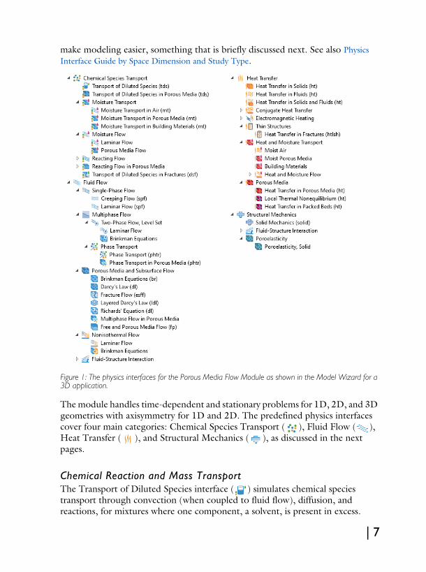
make modeling easier, something that is briefly discussed next. See also Physics Interface Guide by Space Dimension and Study Type.

Figure 1: The physics interfaces for the Porous Media Flow Module as shown in the Model Wizard for a 3D application.

The module handles time-dependent and stationary problems for 1D, 2D, and 3D geometries with axisymmetry for 1D and 2D. The predefined physics interfaces cover four main categories: Chemical Species Transport ( ), Fluid Flow ( ), Heat Transfer ( ), and Structural Mechanics ( ), as discussed in the next pages.

Chemical Reaction and Mass TransportThe Transport of Diluted Species interface ( ) simulates chemical species transport through convection (when coupled to fluid flow), diffusion, and reactions, for mixtures where one component, a solvent, is present in excess.

| 7

The Transport of Diluted Species in Porous Media interface ( ) is tailored to model solute transport in saturated and partially saturated porous media. This physics interface characterizes the rate and transport of individual or multiple and interacting chemical species for systems containing fluids, solids, and gases. The equations supply predefined options to describe mass transfer by convection, adsorption, dispersion, diffusion, volatilization and reactions. You define the convective velocity from either of the included physics interfaces, or you set it to a predefined velocity profile.The Laminar Flow, Diluted Species interface ( ) under the Reacting Flow branch combines the functionality of the Single-Phase Flow and Transport of Diluted Species interfaces. This multiphysics interface is primarily applied to model flow at low to intermediate Reynolds numbers in situations where the mass transport and flow fields are coupled.The Transport of Diluted Species interface ( ) under the Reacting Flow in Porous Media branch combines the Brinkman Equations and the Transport of Diluted Species in Porous Media interfaces. This multiphysics interface is primarily applied to model the transport of diluted reacting mixtures in porous media. The Transport of Diluted Species in Fractures interface ( ) is used to model the transport of a solutes along thin porous fractures, taking into account diffusion, dispersion, convection, and chemical reactions. The fractures are defined by boundaries in 2D and 3D, and the solutes are diluted in a solvent. The mass transport equation solved along the fractures is the tangential differential form of the convection-diffusion-reaction equation. Different effective diffusivity models are available. The Moisture Transport in Building Materials interface ( ) is used to compute the relative humidity field in building materials. It simulates moisture transport by taking in account moisture storage, liquid transport by capillary suction forces.The Moisture Transport in Porous Media interface ( ) is used to compute the relative humidity field in porous media. It simulates moisture transport by vapor convection and diffusion in the gas phase, liquid water transport by convection and capillarity, in the pores of the media. A Hygroscopic Porous Medium feature is active by default on all domains.The Moisture Transport in Air interface ( ) is used to compute the relative humidity distribution in air. It simulates moisture transport by vapor convection and diffusion in moist air and the evaporation or condensation on walls.The Laminar Flow interface ( ) under the Moisture Flow branch combines all features from the Moisture Transport in Air and Single-Phase Flow interfaces. The Moisture Flow multiphysics coupling is automatically added. The fluid properties may depend on vapor concentration. The physics interface supports low Mach numbers (typically less than 0.3). Similarly to Conjugate Heat Transfer coupling,

8 |

the moisture transport interface can be coupled with additional turbulence models for the free flow with the use of the CFD Module.The Porous Media Flow interface ( ) under the Moisture Flow branch combines all features from the Moisture Transport in Porous Media and Brinkman Equations interfaces. The Moisture Flow multiphysics coupling is automatically added. The transport properties may depend on vapor concentration in air. Models can also include moisture transport in building materials.

Fluid FlowFlow in porous media normally occur at low Reynolds numbers. The Reynolds number (Re) is a measure of the ratio of the fluid viscous to the inertial forces acting on the fluid and is given by: Re=ρUL/μ, where ρ is the fluid density, U is a characteristic velocity, L is a characteristic length scale, and μ is the dynamic viscosity. The Creeping Flow interface ( ) approximates the Navier-Stokes equations for the case when the Reynolds number is significantly less than 1. This is often referred to as Stokes flow and it is appropriate for use when viscous flow is dominant.The Laminar Flow interface ( ) describes fluid motion when turbulences are not present, and the Reynolds number is less than approximately 1000. The physics interface solves the Navier-Stokes equations for incompressible, weakly compressible, or compressible flows where the Mach number (Ma) is less than 0.3.The Two-Phase Flow, Level Set interfaces ( ) under the Multiphase Flow branch are used to model two fluids separated by a fluid-fluid interface in a free or a porous medium. The moving interface is tracked in detail using the level set method. The level set method solves additional equations to track the interface location.The Phase Transport interface ( )under the Multiphase Flow branch is used to simulate the transport of multiple immiscible phases in free flow. This interface solves for the averaged volume fractions of the phases.

Porous Media FlowThe Darcy’s Law interface ( ) describes fluid movement through interstices in a porous medium. This physics interface can be used to model low velocity flows, for which the pressure gradient is the major driving force, and the flow is mostly influenced by the frictional resistance within the pores. Its use is within very low flows, or media where the permeability and porosity are very small. You can also set up multiple Darcy’s Law interfaces to model multiphase flows involving more than one mobile phase. The Darcy’s Law interface can also add non-Darcian

| 9

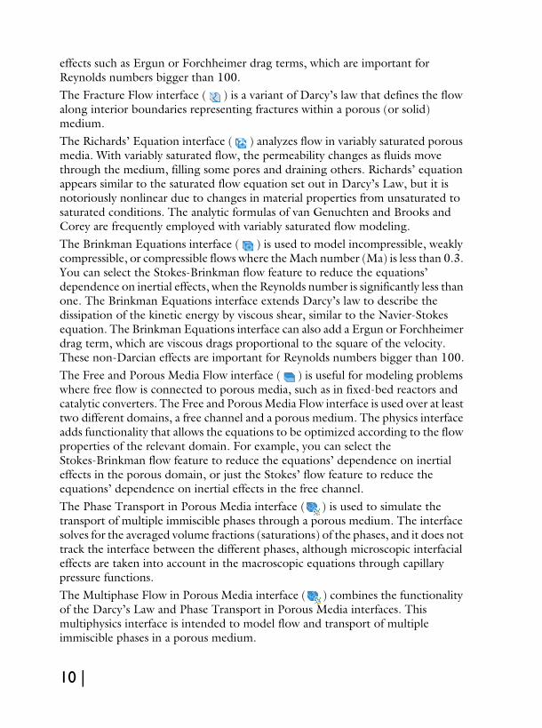
effects such as Ergun or Forchheimer drag terms, which are important for Reynolds numbers bigger than 100.The Fracture Flow interface ( ) is a variant of Darcy’s law that defines the flow along interior boundaries representing fractures within a porous (or solid) medium.The Richards’ Equation interface ( ) analyzes flow in variably saturated porous media. With variably saturated flow, the permeability changes as fluids move through the medium, filling some pores and draining others. Richards’ equation appears similar to the saturated flow equation set out in Darcy’s Law, but it is notoriously nonlinear due to changes in material properties from unsaturated to saturated conditions. The analytic formulas of van Genuchten and Brooks and Corey are frequently employed with variably saturated flow modeling. The Brinkman Equations interface ( ) is used to model incompressible, weakly compressible, or compressible flows where the Mach number (Ma) is less than 0.3. You can select the Stokes-Brinkman flow feature to reduce the equations’ dependence on inertial effects, when the Reynolds number is significantly less than one. The Brinkman Equations interface extends Darcy’s law to describe the dissipation of the kinetic energy by viscous shear, similar to the Navier-Stokes equation. The Brinkman Equations interface can also add a Ergun or Forchheimer drag term, which are viscous drags proportional to the square of the velocity. These non-Darcian effects are important for Reynolds numbers bigger than 100.The Free and Porous Media Flow interface ( ) is useful for modeling problems where free flow is connected to porous media, such as in fixed-bed reactors and catalytic converters. The Free and Porous Media Flow interface is used over at least two different domains, a free channel and a porous medium. The physics interface adds functionality that allows the equations to be optimized according to the flow properties of the relevant domain. For example, you can select the Stokes-Brinkman flow feature to reduce the equations’ dependence on inertial effects in the porous domain, or just the Stokes’ flow feature to reduce the equations’ dependence on inertial effects in the free channel.The Phase Transport in Porous Media interface ( ) is used to simulate the transport of multiple immiscible phases through a porous medium. The interface solves for the averaged volume fractions (saturations) of the phases, and it does not track the interface between the different phases, although microscopic interfacial effects are taken into account in the macroscopic equations through capillary pressure functions.The Multiphase Flow in Porous Media interface ( ) combines the functionality of the Darcy’s Law and Phase Transport in Porous Media interfaces. This multiphysics interface is intended to model flow and transport of multiple immiscible phases in a porous medium.

10 |

As always, the physics interfaces give you direct access to defining, with either constants or expressions, the material properties that describe the porous media flow. This includes the density, dynamic viscosity, permeability, and porosity.

Heat TransferThe Heat Transfer interfaces apply to systems consisting of solids, fluids, and fluid-solid mixtures, and are able to calculate effective properties for porous media consisting of several fluids, gases and solid components, such as a rock formation with different mineral proportions.The Heat Transfer in Solids interface ( ) describes, by default, heat transfer by conduction. The physics interface is also able to account for the heat flux due to translation in solids as well as for solid deformation, including volume or surface changes.The Heat Transfer in Fluids interface ( ) accounts for conduction and convection in gases and liquids as the default heat transfer mechanisms. The coupling to the flow field in the convection term is automatically set when the Nonisothermal Flow multiphysics coupling is used. Otherwise, it may be entered manually in the physics interface, or it may be selected from a list that couples heat transfer to an existing fluid flow interface.The Heat Transfer in Solids and Fluids interface ( ) contains solids and fluids domains by default. It is aimed to simplify the setup of models where capabilities of Heat Transfer in Solids interface ( ) and Heat Transfer in Fluids interface ( ) are used, in particular in conjugate heat transfer applications.The Conjugate Heat Transfer branch ( ) combine features from the Heat Transfer and Single-Phase Flow interfaces to describe heat transfer in solids and fluids and non isothermal flow in fluids. The heat transfer process is tightly coupled with the fluid flow problem via a predefined multiphysics coupling. Additional turbulence models for the free flow are available with the use of the CFD Module.The Heat Transfer in Fractures interface ( ) under the Thin Structures branch ( ) describes heat transfer in fractures and thin porous media. It provides efficient models defined at the boundaries level representing thin three-dimensional domains. The simplest model assumes that the temperature changes through the fracture thickness can be neglected, while the general model computes the temperature variation across the fracture.The Moist Air interface ( ) under the Heat and Moisture Transport branch combines the Heat Transfer in Moist Air interface ( ) with the Moisture Transport in Air interface ( ). It is used to simulate the coupling between heat transfer and vapor transport in air and the evaporation and condensation on walls.

| 11

The Moist Porous Media interface ( ) combines the Heat Transfer in Moist Porous Media and Moisture Transport in Porous Media interfaces. It is used to simulate the coupling between heat transfer and moisture transport in liquid and gas phases in the pores of the medium.The Building Materials interface ( ) combines the Heat Transfer in Building interface ( ) with the Moisture Transport in Building Materials interface ( ). It can be used to model different moisture variations phenomena in building components such as drying of initial construction moisture, condensation due to migration of moisture from outside to inside, or moisture accumulation by interstitial condensation due to diffusion.The Heat Transfer in Porous Media interface ( ) combines the heat conduction and convection in a solid-fluid system. This physics interface provides mixing rules for calculating the effective heat transfer properties, expressions for heat dispersion in porous media. Dispersion is caused by the tortuous path of the liquid in the porous medium, which would not be described if only the mean convective term was taken into account. This physics interface may be used for a wide range of porous materials, from porous structures to the simulation of heat transfer in soils and rocks, and also to model heat transfer in fractures.The Local Thermal Nonequilibrium (LTNE) interface ( ) implements a macroscale model designed to simulate heat transfer in porous media where the temperatures in the porous matrix and the fluid are not in equilibrium. It differs from simpler macroscale models for heat transfer in porous media where the temperature difference of the solid and fluid are neglected. The absence of thermal equilibrium can result from fast transient changes, but it can also be observed in stationary cases. Typical applications are rapid heating or cooling of a porous medium using a hot fluid or internal heat generation in one of the phases (due to inductive or microwave heating, exothermic reactions, and so on). This is observed in nuclear devices, electronics systems, or fuel cells for example.The Heat Transfer in Packed Beds interface ( ) provides a multiscale model for heat transfer in a porous medium where the local thermal equilibrium is not assumed between the pellets of a packed bed and the fluid phase, and where the temperature variation inside the pellets is taken into account. A temperature field is defined for each phase, pellets and fluid of the porous medium, and the heat transfer between them is accounted for. The microscale pellets temperature field depends on the radial coordinate of each pellet.These features interact seamlessly and can be used in combination in a single application. Surface-to-surface radiation can also be included in the energy equation, although this requires a license for the Heat Transfer Module.

12 |

Structural MechanicsThe Poroelasticity multiphysics interface ( ) combines a transient formulation of Darcy’s law with a linear elastic material included in the Solid Mechanics interface. The poroelasticity coupling means that the pore fluid affects the compressibility of the porous medium, as well as changes in volumetric strains affect the porosity and the fluid flow.

Physics Interface Guide by Space Dimension and Study TypeThe table lists the physics interfaces available with this module in addition to those included with the COMSOL Multiphysics basic license.

PHYSICS INTERFACE ICON TAG SPACE DIMENSION

AVAILABLE STUDY TYPE

Chemical Species Transport

Transport of Diluted Species1

tds all dimensions stationary; time dependent

Transport of Diluted Species in Porous Media

tds all dimensions stationary; time dependent

Transport of Diluted Species in Fractures

dsf 3D, 2D, 2D axisymmetric

stationary; time dependent

Moisture Transport

Moisture Transport in Air

mt all dimensions stationary; time dependent

Moisture Transport in Porous Media


Moisture Transport in Building Materials


Moisture Flow

Laminar Flow — 3D, 2D, 2D axisymmetric

stationary; time dependent; stationary, one-way Moisture Flow; time dependent, one-way Moisture Flow

| 13

Porous Media Flow — 3D, 2D, 2D axisymmetric


Reacting Flow

Laminar Flow, Diluted Species1

— 3D, 2D, 2D axisymmetric


Reacting Flow in Porous Media

Transport of Diluted Species

rfds 3D, 2D, 2D axisymmetric


Fluid Flow

Single-Phase Flow

Creeping Flow spf 3D, 2D, 2D axisymmetric


Laminar Flow spf 3D, 2D, 2D axisymmetric


Multiphase Flow

Two-Phase Flow, Level Set

Two-Phase Flow, Level Set, Brinkman Equations


time dependent with initialization

Phase Transport

Phase Transport phtr 3D, 2D, 2D axisymmetric


Phase Transport in Porous Media

phtr 3D, 2D, 2D axisymmetric




14 |

Porous Media and Subsurface Flow

Brinkman Equations br 3D, 2D, 2D axisymmetric


Darcy’s Law dl all dimensions stationary; time dependent

Layered Darcy’s Law ldl 3D stationary; time dependent

Fracture Flow esff 3D, 2D, 2D axisymmetric


Richards’ Equation dl all dimensions stationary; time dependent

Multiphase Flow in Porous Media



Free and Porous Media Flow

fp 3D, 2D, 2D axisymmetric


Nonisothermal Flow

Brinkman Equations — 3D, 2D, 2D axissymmetric

stationary; time dependent; stationary, one-way NITF; time dependent, one-way NITF

Fluid-Structure Interaction

Heat Transfer

Heat Transfer in Solids ht all dimensions stationary; time dependent

Heat Transfer in Fluids1 ht all dimensions stationary; time dependent

Heat Transfer in Solids and Fluids1

ht all dimensions stationary; time dependent

Thin Structures



| 15

Heat Transfer in Fractures

htlsh 3D, 2D, 2D axisymmetric

stationary; time dependent; thermal perturbation, frequency domain

Heat and Moisture Transport

Moist Air — all dimensions stationary; time dependent; thermal perturbation, frequency domain

Moist Porous Media — all dimensions stationary; time dependent; thermal perturbation, frequency domain

Building Materials — all dimensions stationary; time dependent; thermal perturbation, frequency domain

Heat and Moisture Flow

Laminar Flow — 3D, 2D, 2D axisymmetric


Porous Media Flow — 3D, 2D, 2D axisymmetric


Heat Transfer in Porous Media

ht all dimensions stationary; time dependent

Local Thermal Nonequilibrium

ht all dimensions stationary; time dependent; thermal perturbation, frequency domain

Heat Transfer in Packed Beds

ht all dimensions stationary; time dependent; thermal perturbation, frequency domain

Structural Mechanics

Poroelasticity, Solid poro 3D, 2D, 2D axisymmetric




16 |

Poroelasticity, Large Deformation, Solid

poro 3D, 2D, 2D axisymmetric


Poroelasticity, Layered Shell2

— 3D stationary; time dependent

1 This physics interface is included with the core COMSOL package but has added functionality for this module.

2 Requires the addition of the Composite Materials Module and the Structural Mechanics Module.



| 17

Tutorial Model — Packed Bed Latent Heat Storage

Thermal energy storage (TES) units are used to accumulate thermal energy from solar, geothermal, or waste heat sources. The simplest TES units are built from water tanks, where the solar energy is stored as sensible heat. These systems are called sensible heat storage (SHS) units. The thermal capacity of these tanks can be further increased by including latent heat, which gives rise to latent heat storage (LHS) units. Typically, LHS tanks contain spherical capsules filled with paraffin wax as phase change material. Paraffin is a suitable phase change material, as it is relatively inexpensive, reliable and nontoxic, and it is commercially available for a wide range of melting temperatures.This example is inspired by the experimental investigation found in Ref. 1. It models the flow through a packed-bed storage tank, and it includes the effects of heat transfer with phase change and local thermal nonequilibrium (LTNE) while charging the LHS unit.

Figure 2: Latent heat storage unit.

Inlet

Outlet

Glass wool

Spherical capsulesfilled with paraffin

insulation

18 |

MODEL DEFINITION

Paraffin-filled spherical capsules with a diameter of dp = 55 mm are stored in a tank of 36 cm in diameter and 47 cm in height. The porosity of this bed is εp = 0.49. The model geometry is shown in Figure 2.The material properties of paraffin wax are listed in the following table.

Geometry, material properties, and operating conditions are taken from Ref. 1. The initial temperature in the tank is set to 32°C. Warm water flows through the tank with a flow rate of Vin = 2 l/min. During thermal charging the water is continuously heated up by a solar collector that delivers a power of Qu = 375 W. The temperature difference at the tank’s inlet and outlet is given by the relation

(1)

here, Tin and Tout are the inlet and outlet temperatures, and ρ and Cp are the density and heat capacity of water. Ergun equation describes non-Darcian flow through the packed bed, which estimates the pressure drop as a function of the velocity field u

(2)

here, μ (Pa·s) and ρ (kg/m3) are the viscosity and density of water, dp (m) is the spheres’ diameter, and εp the bed porosity. The permeability κ (m2) of the packed bed is given by

(3)

The Reynolds number in the packed bed can be estimated as

(4)

MATERIAL PROPERTY PARAFFIN, SOLID PARAFFIN, LIQUID

Density ρ (kg/m3) 861 778

Heat Capacity, Cp (J/(kg·K)) 1850 2384

Thermal conductivity, k (W/(m·K)) 0.4 0.15

Melting temperature, Tm (°C) 60

Latent heat of fusion, L (J/kg) 213

QuVin-------- ρCp Tin Tout–( )=

∇p μκ---u–

1.75 1 εp–( )

dpεp3

-------------------------------ρ u u–=

κdp

2εp3

150 1 εp–( )2--------------------------------=

Redpvρ

1 εp–( )μ-----------------------=

| 19

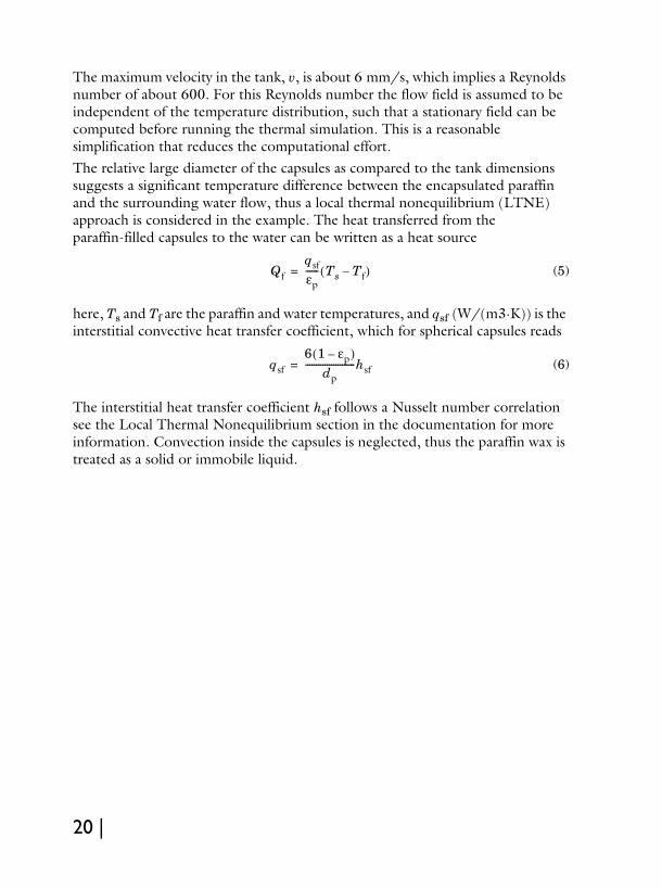
The maximum velocity in the tank, v, is about 6 mm/s, which implies a Reynolds number of about 600. For this Reynolds number the flow field is assumed to be independent of the temperature distribution, such that a stationary field can be computed before running the thermal simulation. This is a reasonable simplification that reduces the computational effort.The relative large diameter of the capsules as compared to the tank dimensions suggests a significant temperature difference between the encapsulated paraffin and the surrounding water flow, thus a local thermal nonequilibrium (LTNE) approach is considered in the example. The heat transferred from the paraffin-filled capsules to the water can be written as a heat source

(5)

here, Ts and Tf are the paraffin and water temperatures, and qsf (W/(m3·K)) is the interstitial convective heat transfer coefficient, which for spherical capsules reads

(6)

The interstitial heat transfer coefficient hsf follows a Nusselt number correlation see the Local Thermal Nonequilibrium section in the documentation for more information. Convection inside the capsules is neglected, thus the paraffin wax is treated as a solid or immobile liquid.

Qfqsfεp------ Ts Tf–( )=

qsf6 1 εp–( )

dp-----------------------hsf=

20 |

RESULTS

The tank reaches a temperature of 70°C after approximately 13 hours. The resulting velocity and temperature distribution is shown in Figure 3.

Figure 3: Velocity field (streamlines) with the gray color indicating the pressure and temperature field (color) after 12 hours of thermal charging.

Figure 4 shows the evolution of the paraffin temperature, water temperature and the weighted average (porous medium) temperature at three different points located in the central axis of the tank. During the phase change, the encapsulated paraffin is not in thermal equilibrium with the surrounding water. Measuring the water temperature alone at the inlet or outlet does not give accurate information about neither the temperature inside the capsules nor the phase in which the paraffin wax is.

| 21

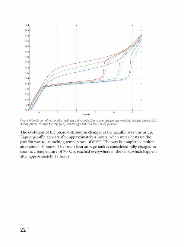
Figure 4: Evolution of water (dashed), paraffin (dotted) and average porous medium temperature (solid) during phase change for top (red), center (green) and low (blue) position.

The evolution of the phase distribution changes as the paraffin wax warms up. Liquid paraffin appears after approximately 4 hours, when water heats up the paraffin wax to its melting temperature of 60°C. The wax is completely molten after about 10 hours. The latent heat storage tank is considered fully charged as soon as a temperature of 70°C is reached everywhere in the tank, which happens after approximately 13 hours.

22 |

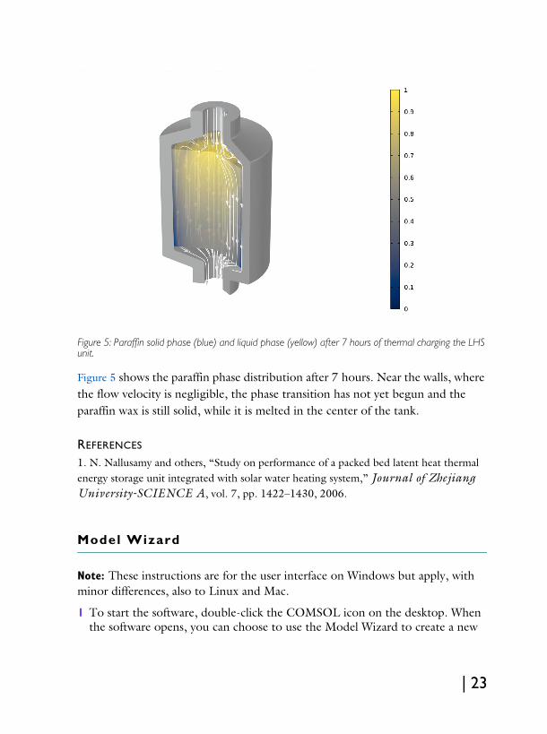
Figure 5: Paraffin solid phase (blue) and liquid phase (yellow) after 7 hours of thermal charging the LHS unit.

Figure 5 shows the paraffin phase distribution after 7 hours. Near the walls, where the flow velocity is negligible, the phase transition has not yet begun and the paraffin wax is still solid, while it is melted in the center of the tank.

REFERENCES

1. N. Nallusamy and others, “Study on performance of a packed bed latent heat thermal energy storage unit integrated with solar water heating system,” Journal of Zhejiang University-SCIENCE A, vol. 7, pp. 1422–1430, 2006.

Model Wizard

Note: These instructions are for the user interface on Windows but apply, with minor differences, also to Linux and Mac.

1 To start the software, double-click the COMSOL icon on the desktop. When the software opens, you can choose to use the Model Wizard to create a new

| 23

COMSOL Multiphysics model or Blank Model . to create one manually. For this tutorial, click the Model Wizard button.If COMSOL Multiphysics is already open, you can start the Model Wizard by selecting New from the File menu and then click Model Wizard .

The Model Wizard guides you through the first steps of setting up a model. The next window lets you select the dimension of the modeling space.

2 In the Select Space Dimension window click 2D Axisymmetric .3 In the Select Physics tree, under Fluid Flow>Porous Media and Subsurface

Flow folder double-click Free and Porous Media Flow to add it to the Added physics interfaces list. You can also click Add or right-click the icon and choose Add Physics .

4 In the Select Physics tree under Heat Transfer, double-click Heat Transfer in Solids and Fluids to add it to the Added physics interfaces list. You can also click Add or right-click and choose Add Physics .

5 Click Study . In the Select Study window under General Studies, click Stationary .

6 Click Done .

Geometry

You can build the geometry from geometric primitives. Here, use instead a file containing the geometry that has been provided for convenience.The location of the file used in this exercise varies based on your installation. For example, if the installation is on your hard drive, the file path might be similar to C:\Program Files\COMSOL\COMSOL60\Multiphysics\applications\. 1 On the Geometry toolbar choose Import .2 In the Settings window for Import, locate the Import section, and browse to

the model’s Application Libraries folder. Double-click the file packed_bed_latent_heat_storage.mphbin.

3 In the Settings window for Import, click Import.

24 |

4 Click Build All Objects to display the geometry.

Global Definit ions — Parameters

Add the parameters needed in this example.

Parameters1 In the Model Builder window under Global Definitions click

Parameters .2 In the Settings window for Parameters enter the following data:

| 25

Materials

Add the material nodes for water, paraffin, and the insulating glass wool. After the physics interfaces have been set up, the software automatically detects which material properties are required and you can fill them in.

Water, liquid1 In the Home toolbar, click Add Material .2 Go to the Add Material window, expand the

Built-in folder and select Water, liquid. Click Add to Component in the window toolbar to add it o the Materials list. You can also double-click on it or right-click and choose Add to Component 1 (comp 1) .

3 On the Home toolbar click Add Material again to close the window.

Paraffin, solid4 In the Model Builder window, under

Component 1 (comp 1) , right-click Materials and choose Blank Material .

5 In the Label text field under the Settings window for Material, type Paraffin, solid.

6 Repeat the last two steps to create two more material nodes, call them Paraffin, liquid and Glass wool respectively.

7 In the Settings window for Glass wool, select Domain 4.8 In the Model Builder window, under Component 1 (comp 1) , right-click

Materials and choose More Materials>Porous Material .9 In the Settings window for Porous Material, select Domain 2 only.The Material node indicates that not all material properties that are required have been defined.

Continue with setting up the physics interfaces and after that you can fill in the required material properties.

26 |


1 In the Model Builder window, under Component 1 click Free and Porous Media Flow .

2 Select Domains 1–3 only. Only in these domains flow will occur.

Porous Medium 11 In the Physics toolbar, click Domains and choose Porous Medium .2 Select Domain 2 only.According to Equation 2, Ergun’s equation gives the best description of the flow behavior in the bed.3 In the Settings window for Porous Medium,

locate the Porous Medium section.4 From the Flow model list, choose Non-Darcian

flow.

Porous Matrix 11 In the Model Builder click Porous Matrix 1.2 In the Settings window for Porous Matrix,

locate the Matrix Properties section.3 From the Permeability model list, choose

Ergun.4 In the dp text field, type dp.

Heat Transfer in Solids and Fluids (ht)

Continue with setting up the heat transfer interface.

Fluid 11 In the Model Builder window, under Component 1>

Heat Transfer in Solids and Fluids click Fluid 1. These are the free flow domains.

2 Select Domains 1 and 3 only.

Initial Values 11 In the Model Builder window, click Initial Values 1.2 In the Settings window locate the Initial Values section.

| 27

3 In the T text field, type T0.

Porous Medium 11 In the Physics toolbar, click Domains and choose Porous Medium .2 Select Domain 2 only.3 In the Settings window for Porous Medium,

locate the Porous Medium section.4 From the Porous medium type list, choose

Local thermal nonequilibrium.5 Choose Spherical pellets from the

Interstitial convective heat transfer coefficient list.

6 In the dpe text field, type dp.

For a porous medium which is not in thermal equilibrium the initial temperatures for each component of the porous medium need to be specified. By default, the fluid phase temperature field is considered to be continuous with the surrounding domains and the solid phase temperature field is considered to be insulated from the surrounding domains.

Initial Values 11 Expand the Heat Transfer in Solids and Fluids>Porous Medium 1>Fluid 1

node, then click Initial Values 1.2 In the Settings window for Initial Values, locate the Initial Values section and

type T0 in the Tf text field.

Porous Matrix 11 In the Model Builder window, under

Heat Transfer in Solids and Fluids> Porous Medium 1 click Porous Matrix 1.

2 In the Settings locate the Matrix Properties section.

3 From the Define list, choose Solid phase properties.

Initial Values 11 Expand the Porous Matrix 1 node, then click Initial Values 1.2 In the Settings window locate the Initial Values section and type T0 in the Ts

text field.

28 |

Phase Change Material 11 In the Model Builder window, click Porous Matrix 1.2 In the Physics toolbar, click Attributes and choose

Phase Change Material .In this solid-solid phase change process, the density is assumed to remain constant which is a reasonable simplification. The mean density value of liquid and solid paraffin is used, which is calculated in the parameter list.

3 In the Settings window locate the Phase Change section and enter:- In the Tpc,1 → 2 text field, type 60[degC].- In the ΔT1 → 2 text field, type 2[K].- In the L1 → 2 text field, type 213[kJ/kg].

4 Locate the Phase 1 section. From the Material, phase 1 list, choose Paraffin, solid (mat2) and from the Material, phase 2 list, choose Paraffin, liquid (mat3).

Multiphysics

Add the multiphysics coupling. After that the software automatically detects which material properties are required for the simulation.1 In the Physics toolbar, click Multiphysics Couplings and choose

Domain>Nonisothermal Flow .

Materials

Paraffin, solid1 In the Model Builder window, under Component 1>Materials click

Paraffin, solid (mat2).

| 29

2 In the Settings window for Material, locate the Material Contents section and enter the following:

Paraffin, liquid1 In the Model Builder window, click Paraffin, liquid.2 In the Settings window for Material, locate the Material Contents section and

in the table enter the following:

Glass Wool1 In the Model Builder window, click Glass Wool.2 In the Settings window for Material, locate the Material Contents section and

enter the following in the table:

Porous Material 1The Porous Material is convenient to use for setting up the material properties for a porous medium that consists of multiple components, typically a fluid and a porous matrix but also multiple solid or fluid phases can be present. In addition pellet structures can be defined and immobile fluid phases can be considered.1 In the Model Builder window, click Porous Material 1.2 In the Settings window for Porous Material, locate the

Phase-Specific Properties section.3 Click Add Required Phase Nodes . This automatically adds a Fluid and Solid

subnode, because these are requested by the physics interfaces.

30 |

Fluid 11 In the Model Builder window, click Fluid 1.2 In the Settings window for Fluid, locate the Fluid Properties section.3 From the Material list, choose Water, liquid (mat1).

Solid 11 In the Model Builder window, click Solid 1.2 In the Settings window for Solid, locate the Solid Properties section.3 In the θs text field, type 1-por.4 Locate the Material Contents section. In the table, enter the following settings:

The next step is to add the boundary conditions for each interface.


In the Model Builder window, under Component 1 click Free and Porous Media Flow .

Inlet 11 In the Physics toolbar, click

Boundaries and choose Inlet.2 Select Boundary 7 only (the top

boundary).3 In the Settings window for Inlet, locate

the Boundary Condition section.4 From the list, choose

Fully developed flow.5 In the Fully Developed Flow section

click the Flow rate button and type V_in in the V0 text field.

Create a selection from this boundary selection. Selections can be used throughout the modeling process and they simplify the assignment of conditions to geometric entities. They are also beneficial for a clear overview.

| 31

6 Locate the Boundary Selection section. Click Create Selection .7 In the Create Selection dialog box, type Inlet in the Selection name text field

and click OK.

This way you have created a selection for the inlet boundary as it will be used again during the model setup. The selections appear under the Component 1>Definitons>Selections node.

Outlet1 In the Physics toolbar, click Boundaries and choose Outlet.2 Select Boundary 2 only.3 In the Settings window for Outlet, locate the Boundary Selection section and

click Create Selection .4 In the Create Selection dialog box, type Outlet in the Selection name text field

and Click OK. Again, this selection for the outlet boundary will be used later in the model setup.

The Free and Porous Media Flow interface is now completely set up.

Heat Transfer in Solids and Fluids

In the Model Builder window, under Component 1 click Heat Transfer in Solids and Fluids .

Inflow 11 In the Physics toolbar, click Boundaries and

choose Inflow.2 In the Settings window for Inflow, locate the

Boundary Selection section and from the Selection list, choose Inlet. Note, that you make use of the selection you have created before.

32 |

3 Locate the Upstream Properties section. In the Tustr text field, type T_in.

The water temperature increases over time during the charging process. While water is pumped through a closed loop, it is heated by a solar system. Therefore you later define the variable T_in as a function of the outlet temperature and the solar heating power using equation Equation 1.

Outflow 11 In the Physics toolbar, click Boundaries and choose Outflow.2 In the Settings window, locate the Boundary Selection section and from the

Selection list, choose Outlet.

Definit ions

The tank is cooled by its surroundings. Create a selection for the outer boundary to apply the heat flux condition.

Heat Flux Boundary1 In the Definitions toolbar, click Explicit .2 In the Settings window for Explicit, type Heat Flux Boundary in the Label text field.

3 Locate the Input Entities section. From the Geometric entity level list, choose Boundary.

4 Select the Group by continuous tangent check box.

5 Select one of the outer boundaries and automatically all boundaries with a continuous tangent will be added to the selection list.

| 33

Heat Transfer in Solids and Fluids (ht)

Heat Flux 11 In the Physics toolbar, click Boundaries and

choose Heat Flux.2 In the Settings window for Heat Flux, locate the

Boundary Selection section.3 From the Selection list, choose Heat Flux Boundary.

4 Locate the Heat Flux section. From the Flux type list, choose Convective heat flux and in the h text field, type 5.

This value is a good approximation to account for cooling by ambient air.

Definit ions

With the next steps you define the variable T_in according to Equation 1.

Average 1Create an average operator to evaluate the temperature at the outlet.1 In the Definitions toolbar click Nonlocal Couplings and choose

Average .2 In the Settings window for Average locate the Source Selection section, and

from the Geometric entity level list choose Boundary.3 From the Selection list, choose Outlet.

Variables 11 In the Model Builder window, right-click Component 1>Definitions and

choose Variables .2 In the Settings window for Variables, locate the Variables section and enter the

following expressions

34 |

The expressions ht.Cp and ht.rho refer to the heat capacity and density of water as defined by the Heat Transfer in Fluids interface.

Mesh 1

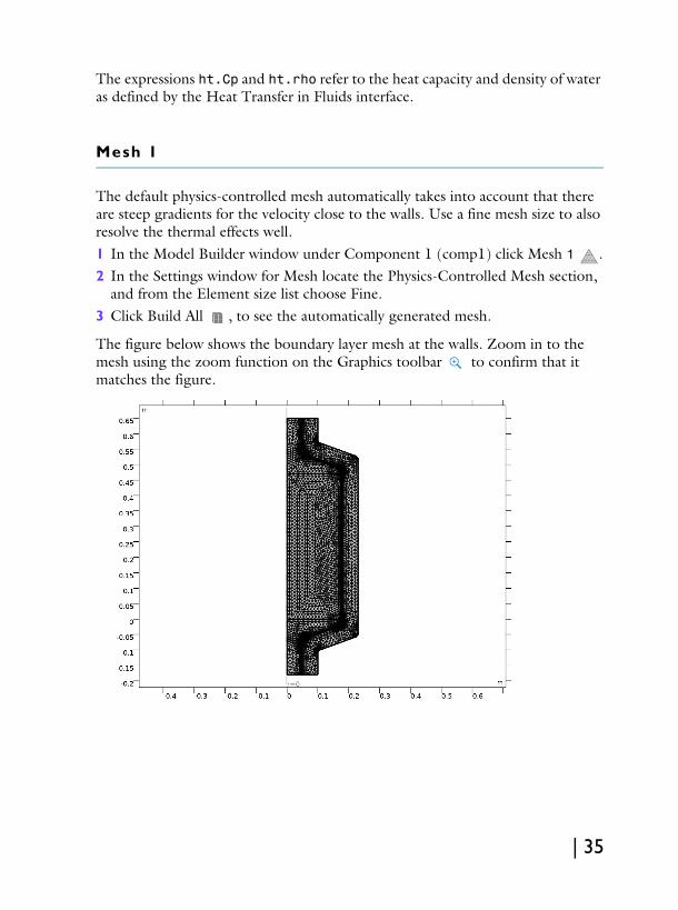
The default physics-controlled mesh automatically takes into account that there are steep gradients for the velocity close to the walls. Use a fine mesh size to also resolve the thermal effects well.1 In the Model Builder window under Component 1 (comp1) click Mesh 1 .2 In the Settings window for Mesh locate the Physics-Controlled Mesh section,

and from the Element size list choose Fine.3 Click Build All , to see the automatically generated mesh.

The figure below shows the boundary layer mesh at the walls. Zoom in to the mesh using the zoom function on the Graphics toolbar to confirm that it matches the figure.

| 35

Study 1

The flow field can be assumed to be independent of time, it is calculated in a first stationary step and then used as input for the heat transport in the subsequent time-dependent step.

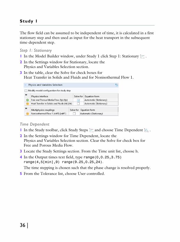
Step 1: Stationary1 In the Model Builder window, under Study 1 click Step 1: Stationary .2 In the Settings window for Stationary, locate the

Physics and Variables Selection section. 3 In the table, clear the Solve for check boxes for

Heat Transfer in Solids and Fluids and for Nonisothermal Flow 1.

Time Dependent1 In the Study toolbar, click Study Steps and choose Time Dependent .2 In the Settings window for Time Dependent, locate the

Physics and Variables Selection section. Clear the Solve for check box for Free and Porous Media Flow.

3 Locate the Study Settings section. From the Time unit list, choose h.4 In the Output times text field, type range(0,0.25,3.75) range(4,5[min],9) range(9.25,0.25,24).The time stepping is chosen such that the phase change is resolved properly.

5 From the Tolerance list, choose User controlled.

36 |

6 In the Relative tolerance text field, type 1e-4.

A tighter tolerance improves the accuracy of the solution which is necessary for resolving all physical effects including the phase change properly.

Solution 1 1 In the Study toolbar, click Show Default Solver .2 In the Model Builder window, expand the Solution 1 node, then click

Time-Dependent Solver 1 .3 In the Settings window for Time-Dependent Solver, click to expand the

Time Stepping section.4 From the Steps taken by solver list, choose Strict.

This forces the solver to use at least the time steps specified above.

Definit ions

Use a stop condition for the time-dependent solver to force the computation to stop when the minimum temperature in the tank reaches 70°C. This requires another coupling operator for the minimum temperature.

Minimum 1 (minop1)1 In the Definitions toolbar, click Nonlocal Couplings and choose

Minimum .2 Select Domain 2 only.

Variables 11 In the Model Builder window, click Variables 1 .

| 37

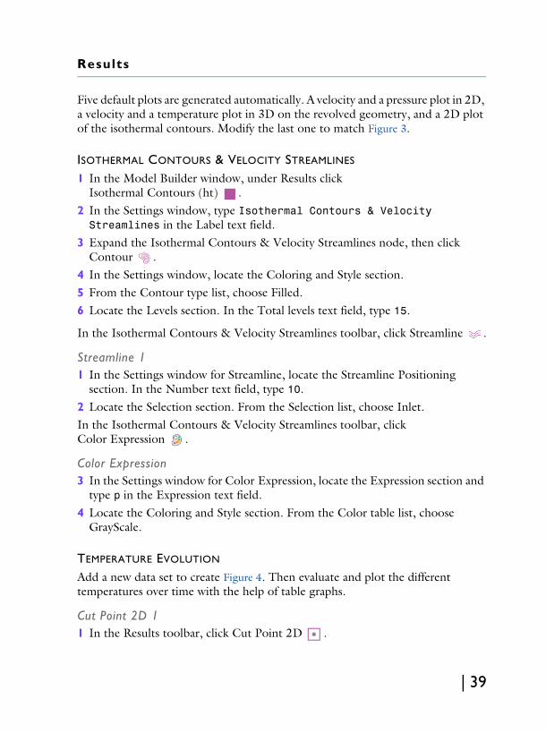
2 In the Settings window for Variables, locate the Variables section and in the table add the new variable T_min.

Study 1

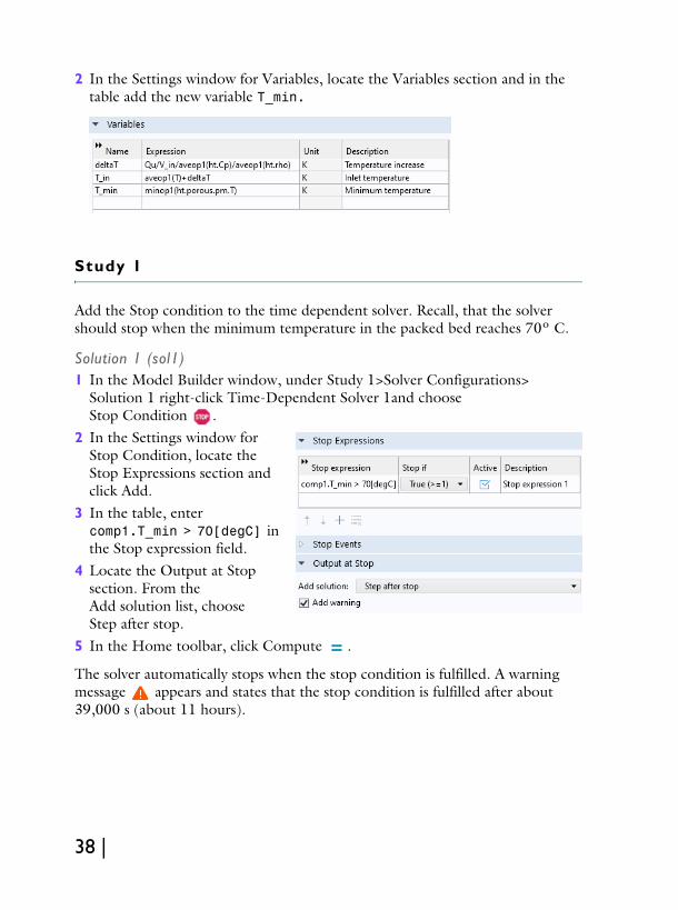
Add the Stop condition to the time dependent solver. Recall, that the solver should stop when the minimum temperature in the packed bed reaches 70º C.

Solution 1 (sol1)1 In the Model Builder window, under Study 1>Solver Configurations>

Solution 1 right-click Time-Dependent Solver 1and choose Stop Condition .

2 In the Settings window for Stop Condition, locate the Stop Expressions section and click Add.

3 In the table, enter comp1.T_min > 70[degC] in the Stop expression field.

4 Locate the Output at Stop section. From the Add solution list, choose Step after stop.

5 In the Home toolbar, click Compute .

The solver automatically stops when the stop condition is fulfilled. A warning message appears and states that the stop condition is fulfilled after about 39,000 s (about 11 hours).

38 |

Results

Five default plots are generated automatically. A velocity and a pressure plot in 2D, a velocity and a temperature plot in 3D on the revolved geometry, and a 2D plot of the isothermal contours. Modify the last one to match Figure 3.

ISOTHERMAL CONTOURS & VELOCITY STREAMLINES

1 In the Model Builder window, under Results click Isothermal Contours (ht) .

2 In the Settings window, type Isothermal Contours & Velocity Streamlines in the Label text field.

3 Expand the Isothermal Contours & Velocity Streamlines node, then click Contour .

4 In the Settings window, locate the Coloring and Style section.5 From the Contour type list, choose Filled.6 Locate the Levels section. In the Total levels text field, type 15.

In the Isothermal Contours & Velocity Streamlines toolbar, click Streamline .

Streamline 11 In the Settings window for Streamline, locate the Streamline Positioning

section. In the Number text field, type 10.2 Locate the Selection section. From the Selection list, choose Inlet.In the Isothermal Contours & Velocity Streamlines toolbar, click Color Expression .

Color Expression3 In the Settings window for Color Expression, locate the Expression section and

type p in the Expression text field.4 Locate the Coloring and Style section. From the Color table list, choose

GrayScale.

TEMPERATURE EVOLUTION

Add a new data set to create Figure 4. Then evaluate and plot the different temperatures over time with the help of table graphs.

Cut Point 2D 11 In the Results toolbar, click Cut Point 2D .

| 39

2 In the Settings window for Cut Point 2D, locate the Point Data section. In the r text field type 0, and in the z text field type 0.05 0.235 0.42. These points will evaluate temperatures in the packed bed at three different positions along the symmetry axis.

Point Evaluation3 In the Results toolbar, click Point Evaluation .4 In the Settings window for Point Evaluation locate the Data section, and from

the Dataset list choose Cut Point 2D 1.5 Locate the Expressions section. In the table enter the following settings:

6 Click Evaluate . A table is created with the data for the temperature variables evaluated at the cut-points for all the time steps.

Table Graph 11 Go to the Table window and click Table Graph in the window toolbar. This

generates a 1D Plot Group 2 node with a Table Graph 1 node.

40 |

2 In the Settings window for Table Graph locate the Data section, and from the Plot columns list choose Manual.

3 In the Columns list choose all entries for the Paraffin temperature.

4 Locate the Coloring and Style section. Find the Line style subsection, and from the Line list choose Dotted.

Table Graph 21 Right-click the Table Graph 1 node and

choose Duplicate .2 In the Settings window for Table Graph

locate the Data section, and in the Columns list choose all entries for the Water temperature.

3 Locate the Coloring and Style section. Find the Line style subsection, and from the Line list choose Dashed. From the Color list choose Cycle (reset).

Table Graph 31 Right-click Table Graph 2 node and choose Duplicate .2 In the Settings window for Table Graph locate the Data section, and in the

Columns list choose all entries for the Porous Medium temperature.

3 Locate the Coloring and Style section. Find the Line style subsection and from the Line list choose Solid.

| 41

1D Plot Group 21 In the Model Builder under Results click 1D Plot Group 2 .2 In the Settings window for 1D Plot Group, type Temperature evolution in

the Label text field to rename the plot.3 Locate the Axis section and select the

Manual axis limits check box. In the x minimum text field, type 3.5, and in the x maximum text field type 9. This zooms into the time range between 3.5 and 9 hours. In the y minimum text field type 328, and in the y maximum text field type 344. to adjust the temperature range.

4 Click Plot in the Temperature evolution toolbar to visualize the data.

You clearly see that paraffin and water are not in thermal equilibrium, especially during phase change of paraffin. Compare with Figure 4.

LIQUID PHASE

With the following steps you can create Figure 5. Learn how to visualize materials in a plot and how to combine different datasets for different entities.

Datasets1 In the Results toolbar, click More Datasets and choose Solution .2 In the Results toolbar, click Attributes and choose Selection .3 In the Settings window for Selection, locate the Geometric Entity Selection

section.4 From the Geometric entity level list, choose Domain and select Domain 4 only.

This is the insulation domain.5 In the Model Builder window, right-click Revolution 2D and choose

Duplicate .6 In the Settings window for Revolution 2D, locate the Data section.7 From the Dataset list, choose Study 1/Solution 1 (3) (sol1) which is the

dataset that you just created.

42 |

3D Plot Group 71 In the Results toolbar, click

3D Plot Group .2 Right-click 3D Plot Group 7 and choose

Volume.3 In the Settings window for Volume enter ht.theta2 in the Expression text field. This is the name of the variable for the phase indicator of phase 2. To find these expressions, click Replace Expression in the upper-right corner of the Expression section. You can then search for expressions or browse through the list.

4 Locate the Coloring and Style section. From the Color table list, choose Cividis.

5 Click to expand the Range section. Select the Manual color range check box.

6 In the Maximum text field, type 1.

Transparency 11 Right-click Volume 1 and choose

Transparency .2 In the Settings window for Transparency,

locate the Transparency section.3 In the Transparency text field, type 0.1.

Volume 21 In the Model Builder window, right-click 3D Plot Group 7 and choose

Volume.2 In the Settings window for Volume, locate the Data section.3 From the Dataset list, choose Revolution 2D 2.4 Locate the Expression section. In the Expression text field, type 1.

Material Appearance 11 Right-click Volume 2 and choose

Material Appearance .2 In the Settings window for

Material Appearance, locate the Appearance section.

| 43

3 From the Appearance list, choose Custom and from the Material type list, choose Aluminum.

Streamline1 In the 3D Plot Group 7 toolbar, click

Streamline .By default the velocity components are used as expressions.

2 In the Settings window for Streamline, locate the Streamline Positioning section.

3 From the Positioning list, choose Uniform density.

4 In the Separating distance text field, type 0.06.

5 Locate the Coloring and Style section. Find the Point style subsection. From the Type list, choose Arrow.

6 Select the Number of arrows check box and in the associated text field, type 120.

7 From the Color list, choose White.

Liquid Phase1 In the Model Builder window,

under Results click 3D Plot Group 7.

2 In the Settings window for 3D Plot Group, type Liquid Phase in the Label text field.

3 Click to expand the Title section. From the Title type list, choose Manual.

4 In the Title text area, type Liquid Phase Saturation (1) and Velocity Streamlines.

5 In the Parameter indicator text field, type Time = eval(t,h) h.

6 Locate the Plot Settings section. Clear the Plot dataset edges check box.7 Locate the Data section. From the Time (h) list, choose 7.

44 |

8 In the Liquid Phase toolbar, click Plot .Use the Plot Previous or Plot Next buttons at the top of the Settings window to plot the results for the previous or next time step respectively. Note, that plotting may take a few seconds.

| 45

46 |

Porous Media Flow Module - COMSOL Documentation

Documents