Pore-scale modeling of hydro-mechanical coupled mechanics ...mechsys.nongnu.org/downloads/wang.2017.pdf · Pore-scale modeling of hydro-mechanical coupled mechanics in hydro-fracturing

Pore-scale modeling of hydro-mechanical coupled mechanics in

hydro-fracturing process

Zhiqiang Chen and Moran Wang†

Department of Engineering Mechanics and CNMM, Tsinghua University, Beijing 100084, China

This paper has been published as: [Z. Chen and M. Wang. Pore-scale modeling of hydro-mechanical coupling mechanics in hydro-fracturing. Journal of Geophysical Research-Solid Earth 122: JB013989, 2017] Abstract: Hydro-fracturing is an important technique in petroleum industry to stimulate well production. Yet the mechanism of induced fracture growth is still not fully understood, which results in some unsatisfactory wells even with hydro-fracturing treatments. In this work we establish a more accurate numerical framework for hydro-mechanical coupling, where the solid deformation and fracturing are modeled by discrete element method (DEM) and the fluid flow is simulated directly by lattice Boltzmann method (LBM) at pore scale. After validations, hydro-fracturing is simulated with consideration on the strength heterogeneity effects on fracture geometry and micro failure mechanism. A modified topological index is proposed to quantify the complexity of fracture geometry. The results show that strength heterogeneity has a significant influence on hydro-fracturing. In heterogeneous samples, the fracturing behavior is crack nucleation around the tip of fracture and connection of it to the main fracture, which is usually accompanied by shear failure. However, in homogeneous ones the fracture growth is achieved by the continuous expansion of the crack, where the tensile failure often dominates. It is the fracturing behavior that makes the fracture geometry in heterogeneous samples is much more complex than that in homogeneous ones. In addition, higher pore pressure leads to more shear failure events for both heterogeneous and homogeneous samples. Keywords: hydraulic fracture, LBM-DEM coupling, fracture geometry, failure mechanism, pore-scale modeling

† Corresponding author: Email: [email protected]; Tel: +86-10-627-87498 1

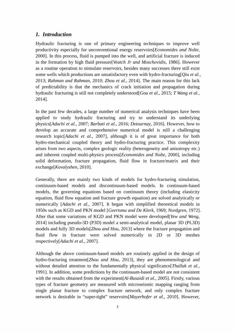
1. Introduction Hydraulic fracturing is one of primary engineering techniques to improve well productivity especially for unconventional energy reservoirs[Economides and Nolte, 2000]. In this process, fluid is pumped into the well, and artificial fracture is induced in the formation by high fluid pressure[Veatch Jr and Moschovidis, 1986]. However as a routine operation to stimulate reservoirs, besides many successes there still exist some wells which productions are unsatisfactory even with hydro-fracturing[Qiu et al., 2013; Rahman and Rahman, 2010; Zhou et al., 2014]. The main reason for this lack of predictability is that the mechanics of crack initiation and propagation during hydraulic fracturing is still not completely understood[Gou et al., 2015; T Wang et al., 2014]. In the past few decades, a large number of numerical analysis techniques have been applied to study hydraulic fracturing and try to understand its underlying physics[Adachi et al., 2007; Barbati et al., 2016; Detournay, 2016]. However, how to develop an accurate and comprehensive numerical model is still a challenging research topic[Adachi et al., 2007], although it is of great importance for both hydro-mechanical coupled theory and hydro-fracturing practice. This complexity arises from two aspects, complex geologic reality (heterogeneity and anisotropy etc.) and inherent coupled multi-physics process[Economides and Nolte, 2000], including solid deformation, fracture propagation, fluid flow in fracture/matrix and their exchange[Kovalyshen, 2010]. Generally, there are mainly two kinds of models for hydro-fracturing simulation, continuum-based models and discontinuum-based models. In continuum-based models, the governing equations based on continuum theory (including elasticity equation, fluid flow equation and fracture growth equation) are solved analytically or numerically [Adachi et al., 2007]. It began with simplified theoretical models in 1950s such as KGD and PKN model [Geertsma and De Klerk, 1969; Nordgren, 1972]. After that some variations of KGD and PKN model were developed[Yew and Weng, 2014] including pseudo-3D (P3D) model a semi-analytical model, planar 3D (PL3D) models and fully 3D models[Zhou and Hou, 2013] where the fracture propagation and fluid flow in fracture were solved numerically in 2D or 3D meshes respectively[Adachi et al., 2007]. Although the above continuum-based models are routinely applied in the design of hydro-fracturing treatment[Zhou and Hou, 2013], they are phenomenological and without detailed attention to the fundamentally physical significance[Thallak et al., 1991]. In addition, some predictions by the continuum-based model are not consistent with the results obtained from the experiment[Al-Busaidi et al., 2005]. Firstly, various types of fracture geometry are measured with microseismic mapping ranging from single planar fracture to complex fracture network, and only complex fracture network is desirable in “super-tight” reservoirs[Mayerhofer et al., 2010]. However,

2

the complexity of the fracture geometry is difficult to be predicted by the continuum-based model owing to its single planar fracture assumption[T Wang et al., 2014]. Secondly, the continuum-based model generally assumes that the failure mode in hydraulic fracturing is the tensile failure, but shear-type seismic events are often recorded in experiments and even in some cases shear failure dominates the fracturing behavior[Falls et al., 1992; Tsuyoshi Ishida et al., 2004]. As an alternative, discontinuum-based models based on discrete element method (DEM) were developed to explore what happened in hydro-fracturing at micro scale[Al-Busaidi et al., 2005; Bruno et al., 2001; Lisjak et al., 2015; Sheng et al., 2015]. In DEM, the rock is regarded as an assembly of bonded particles, which captures the discrete nature of rock effectively and allows for an explicit simulation of the crack nucleation and coalescence. In order to solve the fluid flow in rock, different fluid dynamics modeling methods have been applied to combine hydro-mechanical coupled models with DEM. The first type of models are coarse grid methods[Furtney et al., 2013], where the continuum flow is calculated by solving the Darcy’s law[Bruno et al., 2001] or average NS equations[Eshiet et al., 2013] on the grid larger than the DEM particle. Due to the inconsistent scale for fluid and solid phase in coarse grid methods, empirical formulas are always needed. Another popular type is DEM/pore network coupled model, which has been used to study hydro-fracturing recently and achieved some success[Al-Busaidi et al., 2005; Hazzard et al., 2002; Shimizu et al., 2011]. With simplifications of solid structure (pore and throat) and fluid flow (Poiseuille equation), DEM/pore network model can provide fluid field information at particle scale. However, when the rock breaks up seriously or the void geometry changes dramatically, it is quite difficult to distinguish pore and throat from the DEM structure [Furtney et al., 2013] and the assumption of a same pore pressure value in the fracture is not valid anymore [Ni et al., 2015]. Thus, Ni et al. [2015] simulated hydraulic fracturing with a more accurate pore-scale DEM-CFD coupled model, but it is computationally expensive due to re-meshing at each time step. In the past three decades, the lattice Boltzmann method (LBM) has gained much popularity owing to its efficiency in dealing with complex-boundary. Recently, it has been coupled with DEM to study hydro-mechanical problems in geophysics such as sand production[Boutt et al., 2011; Z Chen et al., 2016]. In LBM-DEM model, fluid flow and fluid-solid interaction are simulated directly and efficiently at pore scale without adjustable parameters[Boutt et al., 2011]. However, only a few LBM-DEM models are applied to simulate hydraulic fracturing, although it is necessary to reveal the mechanism involved. Strength heterogeneity is a common feature in nature rock owing to the pre-existing weak joints, cracks or flaws, which greatly affects the fracture processes and macro mechanical properties[Ma et al., 2014; Ma et al., 2011; Tang et al., 2000], but the role of strength heterogeneity in hydraulic fracturing process has not been fully explored especially quantitatively. In this work, LBM and DEM are coupled to simulate

3

hydraulic fracturing at pore scale, and the effects of strength heterogeneity on fracture complexity and micro failure mechanism are investigated. We try to bridge the gap with a more accurate coupled model, which may help us understand the conflict of failure mode between continuum model prediction and experimental data.

2. Numerical methods and validations

This section gives a brief introduction of numerical methods used in current simulation including lattice Boltzmann method (LBM), discrete element method (DEM) and the LBM-DEM coupling method immersed moving boundary (IMB). Then the LBM-DEM coupled scheme is validated by sphere sedimentation cases.

2.1 Lattice Boltzmann method (LBM)

Lattice Boltzmann method (LBM) is an efficient numerical method to simulate fluid flow, heat and mass transfer especially with complicated boundary condition and multiphase interfaces[M Wang et al., 2007; Z Wang et al., 2016; L Zhang and Wang, 2015]. Recently, LBM has been also widely used to simulate fluid-solid coupling system owing to its high accuracy and efficiency[Boutt et al., 2011; Y Chen et al., 2013; Y Chen et al., 2015; Z Chen et al., 2016]. In LBM, the Boltzmann equation is solved in the discrete lattices, and the obtained macroscopic parameters (velocity, pressure etc.) obey the desired governing equations (such as NS equations) by the Chapman-Enskog expansion[Succi, 2001]. A widespread LBM implementation is the lattice Bhatnagar-Gross-Krook (LBGK) model, where the collision operator is simplified as a linearized version[S Chen and Doolen, 1998] and the evolution equation is written as

( ) ( ) ( ) ( )( )1, , , , , 0 14eqi t t i i if t f t f t f t iδ δ

t+ + = − − = −ix e x x x , (1)

where x denotes the position vector, if is the density distribution in the i-th lattice discrete velocity direction ie , eq

if the corresponding equilibrium distribution, tδ

the time step, t the dimensionless relaxation time related to the fluid kinematic viscosity

( ) 21 23

x

t

t δν

δ−

= , (2)

where xδ is the lattice size. In current simulation, a three-dimensional fifteen-speed model (D3Q15) is applied, which is one of standard and representative models for three-dimensional flows [Qian et al., 1992; M Wang and Chen, 2007]. “D3” indicates three dimension in space and “Q15” means that the density distribution has 15 discrete velocity directions (see Figure 1). In the D3Q15 model, the discrete velocities are

4

0 1 0 1 0 0 0 1 1 1 1 1 1 1 10 0 0 0 0 1 1 1 1 1 1 1 1 1 10 0 1 0 1 0 0 1 1 1 1 1 1 1 1

c− − − − −

= − − − − − − − − − −

e , (3)

where x tc δ δ= . The equilibrium distribution for D3Q15 model is given as

( ) ( )2

2 4 2

93 3, 1+ ,2 2

eqi if

c c cρ ρω

⋅⋅ ⋅= + −

ii e ue u u uu (4)

where the weighting factors are 2 9, 01 9, 1 6

1 72, 7 14i

ii

iω

== = − = −

. (5)

After evolution, the macroscopic density and velocity can be calculated by ,i

ifρ =∑ (6)

ii

fρ =∑ iu e , (7)

and the pressure (p) is given by[S Chen and Doolen, 1998] 21

3p cρ= . (8)

Figure 1. The lattice direction system for D3Q15 model

2.2 Discrete element method (DEM)

Discrete element method (DEM) was proposed in 1979[Cundall and Strack, 1979] and has achieved great success in simulating dynamic behavior of brittle material such as rock. In order to overcome the shape limitation of round particles, the spheropolyhedra method is used in current simulation, where the rock is regarded as an assembly of angular particles[Galindo-Torres et al., 2012], and the current DEM

5

algorithm is based on the MechSys open source library. To model bonding, cohesive forces are assumed at the common face shared by two adjacent particles, which are given by

cohen ncohet t

M AM A

ee

=

=

cohen

cohet

F nF t

, (9)

where cohenF and cohe

tF are cohesive forces in normal and tangential directions respectively, A the shared face area, cohe

nM and cohetM the normal and tangential

elastic modulus of assumed “bond” material, εn and εt the normal and tangential strains of two adjacent particle faces, n and t the unit vectors in normal and tangential directions. When the relative displacements of two adjacent faces reach the threshold value εth

1n t

th

e ee+

> , (10)

the bond will be broken and a small crack forms. In this simulation, the broken bonds are classified as shear failure ( t ne e> ) and tensile failure ( t ne e< ), similar to the classification in [Shimizu et al., 2011]. Besides cohesive forces, another kind of interaction forces are contact forces caused by particle collisions, which are modeled by the normal and shear spring[Cundall and Strack, 1979]. Normal cont

nF and tangential conttF contact forces are proportional to

the overlapping lengths in respective directions

n n

t t

K lK l

= ∆

= ∆

contn

contt

F nF t

, (11)

where Kn and Kt are normal and tangential spring stiffness, nl∆ and tl∆ the overlapping lengths in normal and tangential directions, n and t same as that in Eq. 9. When ,cont cont

t fric nF Fµ> the tangential force becomes contfric nF ,µ=cont

tF t where fricµ the particle friction coefficient, cont

tF and contnF are the magnitude of vector cont

tF and cont

nF . More detail about spheropolyhedra method for DEM simulation can be found in[Galindo-Torres et al., 2012].

2.3 LBM-DEM coupling scheme

For hydro-mechanical coupled model, two aspects must be considered. Firstly, the no-slip boundary condition should be satisfied at the fluid-solid interface. Secondly, hydrodynamic force applied to solid phase need be calculated owing to fluid-solid interaction. In current LBM-DEM model, the immersed moving boundary (IMB) [Noble and Torczynski, 1998] is used to deal with fluid-solid interaction, which offers resolution at the sub-grid scale and allows for accurate and stable calculation of

6

hydrodynamic force [Strack and Cook, 2007]. In IMB, the volume fraction occupied by solid in each cell, namely γ whose value is within [0,1], is obtained, and a fluid-solid interaction term, S

iΩ , is introduced in the evolution equation

( ) ( ) ( ) ( ) ( )( )1, , 1 , ,eq si t t i i i if t f t B f t f t Bδ δ

t+ + = − − − + Ωix e x x x . (12)

The fluid-solid interaction term SiΩ is derived by the bounce-back for

non-equilibrium part

( ) ( ) ( ) ( ), , , ,s eq eqi i i p i i pf t f f t fρ ρ− −

Ω = − − − x v x v , (13)

where vp is the solid velocity at position x. In Eq. 12, B is a weight function depending on γ in each cell

( )( ) ( )

0.51 0.5

Bγ tγ t

−=

− + −. (14)

When γ=0, B=0; and γ=1, B=1. It means that the evolution equation (Eq. 12) can recover the standard LB equation and bounce-back rule for γ=0 and 1, respectively. The hydrodynamic force exerted on the DEM particle is calculated by the change of momentum in all cells covered by the particle

3sx

n i in it

Bδδ

Ω

∑ ∑F = e , (15)

where n is the number of cells covered by the DEM particle. The torque T can be calculated similarly

( )3

sxn cm n i i

n it

Bδδ

− Ω

∑ ∑T = x x e , (16)

where xn is the cell position, and xcm is the mass center of the DEM particle.

2.4 Validations

To validate the current LBM-DEM scheme for fluid-solid coupling problems, two benchmark cases are considered, single-sphere sedimentation and two-sphere sedimentation. Because results of direct numerical simulations for sphere sedimentations have been presented in many previous papers using FEM or other methods [Y Chen et al., 2015; Glowinski et al., 2001; Sharma and Patankar, 2005; Strack and Cook, 2007], there is sufficient data available for validation.

2.4.1 Single-sphere sedimentation

For a single offset sphere settling down in a column of fluid, it will oscillate around the centerline of the column with decreasing amplitude[Strack and Cook, 2007]. Eventually, a fixed settling velocity is achieved with no lateral motion. Based on this velocity, the terminal particle Reynolds number is calculated

7

Re udν

= , (17)

where u is sphere terminal velocity, d the sphere diameter, and ν is the kinematic viscosity. For comparison, the channel and sphere geometry are set as same as that in [Strack and Cook, 2007]. A sphere with diameter d is placed in a square channel L L× wide and 16 L deep ( 3 2L d= ). The initial sphere position is 0.4 L from the side of column in x direction (see Figure 2a). By adjusting the value of gravity, different terminal particle Reynolds can be achieved. In this case Re=15, the sphere trajectories obtained by present LBM-DEM model agree well with that in [Strack and Cook, 2007].

Figure 2. (a) The geometry of single sphere sedimentation benchmark case, where a sphere (d=2/3 L) is placed in 0.4 L from the side of column in x direction. (b) The trajectory of sphere in current simulation agrees well with that in [Strack and Cook, 2007].

2.4.2 Two-sphere sedimentation

When two separated spheres settle down at zero initial velocity (see Figure 3), a famous phenomenon so-called “drafting, kissing and tumbling” or DKT motion will occur[Fortes et al., 1987]. “Drafting” in this process means the trailing sphere will accelerate due to the low pressure in the wake of the leading one. Then it catches the leading sphere, and “kissing” motion happens. Owing to the instability of contacting spheres aligned in the settling direction, they tend to “tumble” to another position. As a result, the relative position of two spheres exchanges and the initial trailing sphere becomes the leading one. We also simulate this process for further validation, where two spheres with density 1.14 g/cm3 and radius 0.083 cm settle down under gravity in a column with square cross section 1 1cm cm× and 4 cm depth (see Figure 3a). The centers of two spheres

0.4

0.43

0.46

0.49

0.52

0.55

0 4 8 12 16

X/L

Z/L

Current SimulationStrack et.al 2007

(a) (b)

8

are located at (0.5 cm 0.5 cm 3.4 cm) and (0.5 cm 0.5 cm 3.16 cm) initially. The fluid kinematic viscosity is 0.01 m2/s and density is 1 g/cm3. The same case was also modeled in [Glowinski et al., 2001] using FEM and [Sharma and Patankar, 2005] with FVM. Figure 3b shows the vertical positions of two spheres during the sedimentation process, and up to the “kissing” stage, our results agree well with that in[Glowinski et al., 2001; Sharma and Patankar, 2005]. After the kissing stage, exact agreement is not expected, because the “tumbling” is the realization of an instability, and different particles collision models will lead to different motions after “kissing”[Glowinski et al., 2001; Sharma and Patankar, 2005].

Figure 3. (a) The geometry of two spheres sedimentation benchmark case, where two spheres with radius 0.083 cm settle down under gravity in a square channel with cross section 1 1cm cm× and depth 4 cm. (b) The vertical positions of two spheres during sedimentation process obtained from different simulations, and our results agree well with others.

3. Hydro-fracturing simulation

3.1 Physical Model and Modeling Parameters

The rock sample in current hydro-fracturing simulation is presented in Figure 4a, where a hole is set at the middle of the left edge for fluid injection. For hydro-fracturing simulation, the rock sample is firstly discretized as an assembly of triangular solid particles (see Figure 4c). To simulate the flow behavior in the rock, the triangular particles in Figure 4c are eroded by a small distance to obtain the “flow channel” (see Figure 4d), which is a common numerical approach to deal with fluid-solid coupling process[Boutt et al., 2011; Shimizu et al., 2011]. In Figure 4d, the triangular particle is regarded as impermeable, and the fluid can only flow along the triangular grain boundary namely “flow channel”, which provides the primary

0

0.008

0.016

0.024

0.032

0.04

0 0.1 0.2 0.3 0.4 0.5 0.6

Verti

cal p

ositi

on (m

)

Time (s)

Current Simulation Sphere2Current Simulation Sphere1Glowinski 2001 Sphere 1Glowinski 2001 Sphere2Patankar 2005 Sphere2Patankar 2005 Sphere1

(a) (b)

9

permeability for the rock matrix just like [Boutt et al., 2011] for sand production simulation. This idealization can be thought of two triangular particles in Figure 4d being separated by a virtual bond beam, which supports particles interaction force and is permeable to fluid. Current model is a pseudo-2D model for the sake of simplicity and computation time, and only one layer of particles are considered, but it can be extended to fully 3D case without difficulty.

Figure 4. Physical model and computational system for simulations. (a) The rock sample used for hydro-fracturing simulation, where a hole is set in the middle part of left edge for fluid injection. (b) Discretization of rock sample by triangular particles with same thickness in DEM. (c) The 2D projection diagram from thickness direction. (d) Two triangular DEM particles are bonded together by virtual bond beam, which serves as the flow channel for fluid.

3.1.1 Fracture dependent flow conductivity

For fluid flow in deforming fractured rocks, an important character is the fracture-controlled fluid flow[Latham et al., 2013; Nick et al., 2011; Yardley, 1983; X Zhang et al., 2002], which means new formed cracks are much more permeable than the matrix primary permeability. If a connected fracture is formed, it will dominate the flow behavior in the rock[X Zhang et al., 2002]. Thus the crack propagation and the fluid flow is a strong two-way coupling process. However, previous LBM-DEM schemes did not consider this effect, and when the bond was broken, the flow conductivity did not change at all. In order to capture this feature, immersed moving boundary (IMB) is also introduced in the “flow channel”. When the bond is intact, an initial volume fraction (γ <1) is set for the LBM cells in the “flow channel”, which means the “flow channel” is partly occupied by the virtual stationary solid, corresponding to a low flow conductivity. By changing the initial value of γ, different rock matrix permeability can be achieved, and larger γ results in lower rock primary permeability. During the hydro-fracturing

(a) (b)

(c) (d)

10

simulation, the γ of LBM cells in smaller triangular particles (see Figure 4d) is updated at each time step by calculating the volume fraction occupied by solid. The γ of LBM cells in the “flow channel” keeps the initial constant value as long as the bond is intact. When the bond is broken (new crack forming), γ in the corresponding “flow channel” is set to 0, which means flow resistance caused by virtual stationary solid is removed by the formation of crack. As a result, the flow conductivity enhanced by fracture can be captured effectively.

3.1.2 Characterization of strength heterogeneity

Strength heterogeneity is a common feature in rock material and can be quantitatively evaluated by Weibull distribution[McClintock and Zaverl Jr, 1979; Rossi and Richer, 1987]. In current model, the strength heterogeneity of the sample is achieved numerically by setting bonding strength threshold (εth) in a random manner following the Weibull distribution

( )1

0 0 0expm m

th thth

th th th

mf e eee e e

− = −

, (18)

which is a common approach to represent the strength heterogeneity in geo-materials, and has obtained some satisfactory simulation results and good consistency with experiments[Mahabadi et al., 2014; Zhu and Bruhns, 2008]. However, it should be noticed that the two parameters in the Weibull function need to be determined statistically case by case for different kinds of rocks. In Eq. 18, 0

the is the average bonding strength threshold, and m>0 is the shape parameter describing the dispersion degree of the . With increasing m, the generated data ( the ) are more concentrated. Hence, in previous study m was often used to quantify the heterogeneity degree[Ma et al., 2011], but it is not intuitive owing to the nonlinear relation between m and heterogeneity degree. In this work, a heterogeneity index hs is suggested to quantify the strength heterogeneity, whose value equals the relative standard deviation/coefficient of variation of Weibull distribution with shape parameter m

( )( ) ( )( )2

1 1

1 2 1 1std

smean

mh

E m m

s Γ += =

Γ + − Γ +, (19)

where Г is gamma function, stds the standard deviation, meanE the mean value. As expected, heterogeneity index hs only depends on the shape parameter m as shown in Figure 5a. For all m>1, hs is between 1 and 0. When m=1, hs=1 corresponding to a high degree of heterogeneity. With increasing m, hs decreases rapidly initially and then slows down (see Figure 5a). When , 0sm h→∞ → , and completely concentrated data are generated with no heterogeneity. Consequently, hs gives an intuitive and general quantification of heterogeneity degree and can also be extended to other distributions.

11

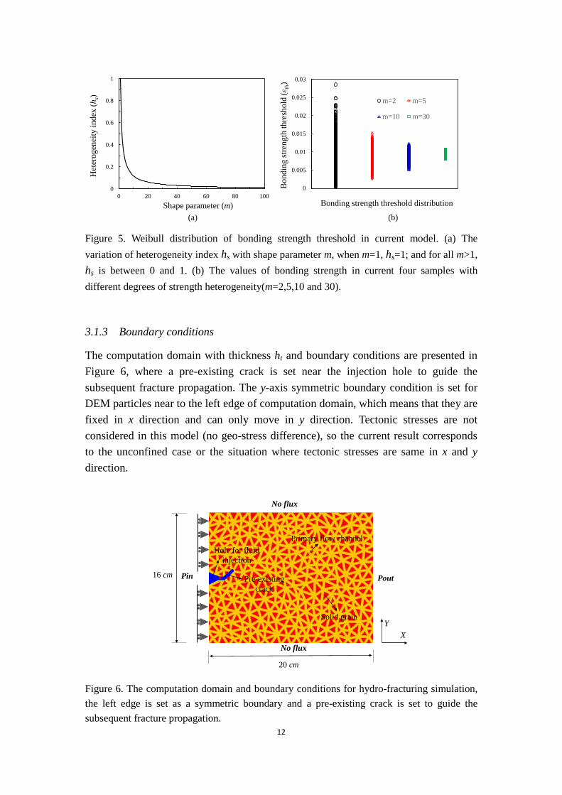
Figure 5. Weibull distribution of bonding strength threshold in current model. (a) The variation of heterogeneity index hs with shape parameter m, when m=1, hs=1; and for all m>1, hs is between 0 and 1. (b) The values of bonding strength in current four samples with different degrees of strength heterogeneity(m=2,5,10 and 30).

3.1.3 Boundary conditions

The computation domain with thickness ht and boundary conditions are presented in Figure 6, where a pre-existing crack is set near the injection hole to guide the subsequent fracture propagation. The y-axis symmetric boundary condition is set for DEM particles near to the left edge of computation domain, which means that they are fixed in x direction and can only move in y direction. Tectonic stresses are not considered in this model (no geo-stress difference), so the current result corresponds to the unconfined case or the situation where tectonic stresses are same in x and y direction.

Figure 6. The computation domain and boundary conditions for hydro-fracturing simulation, the left edge is set as a symmetric boundary and a pre-existing crack is set to guide the subsequent fracture propagation.

0

0.2

0.4

0.6

0.8

1

0 20 40 60 80 100

Het

erog

enei

ty in

dex

(hs)

Shape parameter (m)

0

0.005

0.01

0.015

0.02

0.025

0.03

Bon

ding

stre

ngth

thre

shol

d (ε

th)

Bonding strength threshold distribution

m=2 m=5

m=10 m=30

(a) (b)

20 cm

Pout

XY

No flux

No flux

16 cm Pin

Primary flow channel

Solid grain

Hole for fluid injection

Pre-existing crack

12

The current DEM parameters summarized in Table 1 are chosen with the consideration of computation expense, and no attempt was made to match exact macro-mechanical properties of the real rock. We may be allowed to do this, because our present objective is to show the significant effects of strength heterogeneity on hydro-fracturing with a more accurate hydro-mechanical coupled model, and the results are not influenced by the specific macro properties. To explore the effect of strength heterogeneity, we prepare four kinds of samples with different heterogeneity degrees, whose average bonding strength threshold 0

the =0.01 and heterogeneity index hs=0.52, 0.23, 0.12 and 0.04 (m=2, 5, 10 and 30), respectively (see Figure 5b). In this simulation, 503 triangular elements and 659 contact elements are used, which are considered sufficient to represent the Weibull distribution[Rossi and Richer, 1987].The discussion on the mesh-independence of current simulation results is provided in Appendix II.

Table 1. DEM parameters in current model

Parameter Value Normal stiffness, Kn 52.1 10 N m×

Tangential stiffness, Kt 51.4 10 N m× Particle friction coefficient, μfric 0.4 Average bonding strength, 0

the 0.01 Solid particle density, sρ 3 35.0 10 kg m×

Normal elastic modulus, cohenM 61.75 10 Pa×

Tangential elastic modulus, cohetM 61.75 10 Pa×

Particle thickness, ht 4.8 mm To induce hydraulic fracture, a constant high injection pressure is applied initially at the left side of the hole (the middle of the left vertical edge), and a low fluid pressure is kept at the right edge. It is a common fluid boundary condition for hydro-fracturing simulation, because the constant injection pressure was preferred over the constant flow rate in experiments[Al-Busaidi et al., 2005]. The bottom and top edges are no flux boundary conditions for fluid. The fluid parameters and their implementation in LBM are listed in Table 2. Here the D3Q15 model is used, and the lattice size xδ is

44.0 10 m−× , and the 3D lattice number is 500 400 12× × . The time step tδ in LBM and DEM are same and equal to 61.33 10 s−× , which corresponds to a relatively high lattice velocity, so the deleterious compressibility can be annihilated. The width of “flow channel” (see Figure 6) in current simulation is 2.4 mm. In order to get a more general conclusion, four inlet pressures are considered ( in outP P− =120, 180, 240 or 300 kPa), which are all high to induce fracture but low enough to maintain stability.

13

Table 2. Fluid parameters and their LBM implementation

Parameter Value Fluid density, fρ 331 10 kg m×

Fluid kinematic viscosity, ν 3 22.0 10 m s−× Grid size in LBM, xδ 44.0 10 m−×

Time step in LBM and DEM, tδ 61.33 10 s−× Channel initial solid volume fraction, γ 0.8

3.2 Results and Discussion

The present numerical modeling results will be compared with the available experimental data and the fracturing mechanism will be discussed in this sub-section. Firstly, the strength heterogeneity effect on fracture geometry is presented, which shows how the rock mass property influences the hydraulic fracture. Then in order to explain this heterogeneity effect, fracturing behavior and micro failure mechanism are investigated at micro scale. Finally, the quantitative descriptions of fracture geometry and failure mechanism under various pressure differences are presented, which helps to provide a comprehensive understanding of the heterogeneity effect on hydro-fracturing.

3.2.1 Validation of pressure evolution

Before exploring the strength heterogeneity effect, current model is further validated by recording the pressure evolution in the hole. The physical model is same as that in Figure 6, and the fixed velocity and pressure boundary conditions are applied to the inlet and outlet of the computation domain, respectively. The pressure in the hole (red point in Figure 6 (1.75 cm, 8.0 cm)) is recorded during the simulation, and the evolution of dimensionless pressure increment in this point is plotted in Figure 7 (normalized by the maximal pressure increment). It is presented that current LBM-DEM model successfully captures the pressure fluctuation during the fracture propagation (see Figure 7a), a typical pressure behavior in hydraulic fracturing tests, which is very consistent with the measured data from experiments [Cornet and Valette, 1984; Economides and Nolte, 2000]. It is because our model introduces the fracture dependent flow conductivity. When the flow conductivity becomes fracture independent, like the previous LBM-DEM models did, the pressure response with time becomes monotonically increasing, as shown in Figure 7b, which is consistent with the previous LBM-DEM modeling results. Hence, the current model is available to be further used to study the heterogeneity effect on hydro-fracturing.

14

Figure 7. Pressure evolution curve by different methods. (a) Pressure evolution in current model where the flow conductivity enhanced by new fracture is considered. It captures the pressure fluctuation owing to crack propagation, a typical feature in hydro-fracturing test, and consistent with the measured data from experiments [Cornet and Valette, 1984; Economides and Nolte, 2000]. (b) The pressure evolution predicted when the flow conductivity becomes fracture independent like in previous LBM-DEM scheme, which fails to capture this behavior.

3.2.2 Strength heterogeneity effect on hydro-fracturing

In hydro-fracturing operation, fracture geometry is an essential parameter to evaluate its efficiency[Mayerhofer et al., 2010]. In the conventional reservoir, simple fracture such as single plane fracture is enough, but for an unconventional reservoir only a complex fracture network can improve its production[Mayerhofer et al., 2010]. Consequently it is of great necessary to explore the relationship between rock mass properties and the hydraulic fracture geometry, so that we can predict what kind of fracture geometry tends to be generated in a specific reservoir. Recently, some rock properties such as brittleness[Chong et al., 2010] and geologic discontinuities [Warpinski and Teufel, 1987] have been studied, but the effect of the strength heterogeneity ,a common but essential feature in rock, on the fracture geometry has not been fully investigated especially quantitatively. Thus we attempt to bridge this gap with current simulation. The numerical modeling results of hydraulic fracture geometry in the synthetic samples with different degrees of heterogeneity are presented in Figure 8a-8d, which demonstrate that strength heterogeneity has a significant effect on the complexity of hydraulic fracture. Figure 8a shows the hydraulic fracture in highly heterogeneous sample (hs=0.52), where many branches are generated and widely scattered in the formation, corresponding to a complex fracture geometry. However, for homogeneous sample (hs=0.04), the fracture geometry is much simpler and few branches are observed (see Figure 8d). Figure 8b and 8c show the fracture geometry in samples

0

0.3

0.6

0.9

1.2

0 1.5 3 4.5 6

Dim

ensi

onle

ss p

ress

ure

Dimensionless time

0

0.3

0.6

0.9

1.2

0 1 2 3 4 5

Dim

ensi

onle

ss p

ress

ure

Dimensionless time(a) (b)

15

with middle degree of heterogeneity, and their fracture complexity also lies within the above two extremes. Because the tectonic stress is not included in current model, there is no predominant direction for fracture propagation just as the unconfined hydro-fracturing test[Falls et al., 1992]. Another obvious difference between heterogeneous and homogeneous samples is that, in highly heterogeneous sample a lot of isolated small cracks are formed, which are not coalesced to the main fracture(see Figure 8a). However, few isolated cracks are found in homogeneous one (see Figure 8d). Figure 8e-8h show the fluid field corresponding to the fracture geometry in Figure 8a-8d. As expected, the fracture new induced is more permeable than the surrounding rock formation, and when a connected fracture is formed, it dominates the flow behavior.

Figure 8. The fracture geometry under the pressure difference 240 kPa, with different heterogeneity index: (a) hs=0.52, which corresponds to a highly heterogeneous sample; (b) hs=0.23; (c) hs=0.12; (d) hs=0.04, a nearly homogeneous sample. Color contours (e)-(h) are the flow fields corresponding to the rock samples in (a)-(d). This kind of feature has also been observed in a recent hydro-fracturing experiment[P Liu et al., 2016] (see Figure 9). Figure 9a shows the hydraulic fracture in an artifical heterogeneous sample, which is more complex than the fracture in homogeneous one (Figure 9b). The experimental results in Figure 9 are obtained under the no geo-stress difference test condition just like current simulation. As a comparison, our results are also presented (see Figure 9c and 9d). The experimental fracture geometry of heterogeneous rock is similar to our simulation result in heterogeneous sample with hs=0.23, and the simple fracture in homogeneous rock is similar to that in current homegeneous sample with hs=0.04.

(a) (b)

(c) (d)

(e) (f)

(g) (h)

16

Figure 9. The hydraulic fracture geometry in different rock samples, where (a) and (b) are artificially heterogeneous and homogeneous samples respectively from Ref. [P Liu et al., 2016]. (c) The fracture geometry in current heterogeneous sample with hs=0.23. (d) The hydraulic fracture in homogeneous sample with hs=0.04.

3.2.2.1 Fracture propagation patterns

In order to understand this heterogeneity controlled behavior at micro scale, the fracturing behaviors in heterogeneous and homogeneous samples are presented. The sample with hs=0.23 is taken as an example to show the fracture growth in heterogeneous rock (see Figure 10). When the fluid with high pressure is injected, the crack is firstly induced around the borehole (see Figure 10a). As the fracture propagates, some scattered micro cracks around the main fracture is generated (see Figure 10b-10d). It is because that in heterogeneous rock, bonding strength (εth) distribution is within a large range, and some weak bonds exist (see Figure 5b), which are easily broken by shear force (see Figure 10j) being the small crack nucleation. Then these crack nucleation may interact and coalesce, and finally be connected to the main fracture forming new branches. As a result, a complex hydraulic fracture is induced. Hence, the fracturing behavior in heterogeneous rock can be summarized as the nucleation and coalescence of the small cracks. It is this particular fracturing behavior that results in the complexity of the hydraulic fracture. However, in continuum-based model, the fracture propagation is often regarded as a continuous expansion process based on linear elastic fracture mechanics (LEFM), so it is difficult to capture this discontinuous pattern of crack propagation.

(a)

(b)

(c)

(d)

17

Figure 10. Analysis of fracture propagation patterns in heterogeneous rock. (a)-(i) The fracture propagation process in heterogeneous rock with hs=0.23 under the pressure difference of 240 kPa, which can be summarized as the formation and coalescence of crack nucleation. (j) The failure mode for each crack, where red and blue dots indicate the bond broken by tensile failure and shear failure, respectively. Contrary to the heterogeneous case, fracture propagation in homogeneous sample is achieved by continuous crack expansion with few branches (see Figure 11), which is consistent with the traditional continuum theory. This is possibly due to the small range of bonding strength (εth) distribution in homogeneous sample, and few weak bonds exist to form crack nucleation around the main fracture. Consequently, only a simple fracture is induced in the homogeneous sample.

Figure 11. Analysis of fracture propagation patterns in homogeneous rock. (a)-(i) The fracture propagation process in homogeneous rock with hs=0.04 under the pressure difference of 240 kPa, where the fracture growth is achieved by continuous expansion of crack and corresponds to a simple fracture geometry with few branches. (j) Failure mode for each crack, where red and blue dots are the bonds broken by tensile failure and shear failure, respectively.

(a)

Blue: small crack caused by shear failure;

Red: small crack caused by tensile failure;The size of dot represents the magnitude of bonding strength for each small crack.

Weak bond

(b) (c)

(d) (e) (f)

(g) (h) (i) (j)

(a)

Blue: small crack caused by shear failure;

Red: small crack caused by tensile failure;The size of circle represents the magnitude of bonding strength for each small crack.

(b) (c)

(d) (e) (f)

(g) (h) (i) (j)

18

3.2.2.2 Micro-failure mechanism

Over the past few decades, acoustic emissions in laboratory and field scale have been recorded to clarify the micro-failure mechanism of hydraulic fracture[Falls et al., 1992; Stoeckhert et al., 2015; Talebi and Cornet, 1987], and one of the major findings is that shear failure seismicity is commonly recorded and even in some cases it dominates the failure behavior[Al-Busaidi et al., 2005]. However, this observation is not consistent with tensile fracture suggested by traditional analytical and numerical models, and the conflict has not been fully solved[Al-Busaidi et al., 2005; T Ishida et al., 1997; Shimizu et al., 2011]. In current simulation, shear failure events are also observed (see Figure 10j and 11j) just as experimental observations. Figure 12 shows the variation of shear and tensile failure events during hydro-fracturing. It is presented that strength heterogeneity also has an influence on micro-failure mechanism. Shear failure dominates the fracturing behavior in the heterogeneous sample (see Figure 12a), but in the homogeneous sample tensile failure events more easily occur (see Figure 12b). Similar scenarios can also be found in a recent hydro-fracturing experiment[Stoeckhert et al., 2015]. For a deep understanding of this phenomenon, fracture propagation pattern and micro-failure mechanism are analyzed simultaneously. It is presented that shear failure is usually accompanied by forming crack nucleation and connecting it to the main fracture, which more easily happens in heterogeneous rock (see Figure 10j). Similar results about the role of shear failure in hydro-fracturing were also obtained by laboratory and field experiments [Tsuyoshi Ishida, 2001; Talebi and Cornet, 1987]. In contrary, tensile failure events are often accompanied by continuous expansion of the crack (see Figure 11j), which is commonly observed in homogeneous rock. The above discussion may help us understand the conflict between experimental observations and continuum theory predictions. In continuum model, it is usually assumed that the fracture propagation is achieved by continuous expansion of the crack, and under this condition tensile fracturing is indeed the main failure mechanism just as presented in the homogeneous sample (Figure 11j). However this assumption may be no longer valid in real rock with high heterogeneity degree, where the fracture propagation is not continuous and often accompanied by shear failure. Thus the traditional model cannot effectively predict the fracturing behavior and failure mechanism in real rock.

19

Figure 12. Variation of shear and tensile failure events in (a) heterogeneous sample (hs=0.23) and (b) homogeneous sample (hs=0.04) under the pressure difference of 240 kPa.

3.2.3 Quantitative description of fracture geometry and failure mechanism

The above discussions are mainly qualitative and under the pressure difference of 240 kPa. In this sub-section, quantitative descriptions of fracture geometry and failure mechanism with various pressure differences (120 kPa, 180 kPa, 240 kPa and 300 kPa) are considered, which helps to provide a comprehensive understanding of the heterogeneity effect on hydro-fracturing. Quantitative analysis of fracture geometry is an important aspect of studying the cracking behavior of rock[C Liu et al., 2013] and evaluating the hydro-fracturing operation[Mayerhofer et al., 2010]. However, owing to the complexity of fracture geometry, current analysis is still limited to the quantification of basic geometric parameters of the fracture such as fracture length, fracture density and fractal dimension[C Liu et al., 2013], and none of them can reflect the morphology of fracture geometry directly and effectively. Thus, how to define an index to quantify the fracture geometry is of great significance but also difficult. In current simulation, the hydraulic fracture is mainly a “tree” type fracture. Consequently, the topological index (q) for “tree” type structure is introduced to quantify the hydraulic fracture in current simulation, which was originally used to describe the geometry of root system [Bouma et al., 2001; Oppelt et al., 2001]. In root system, there are two extreme structures, herringbone branching (Figure 13a) and dichotomous branching (Figure 13b). Herringbone branching is a simple structure with low degree of the branching growth and development. On the contrary, dichotomous branching corresponds to a high degree of the branching growth, and can be regarded as an ideal hydraulic fracture with high geometric complexity. The topological index (q) is such a parameter to quantify branching patterns between the above two extremes[Oppelt et al., 2001]. When q=0, the fracture corresponds to the dichotomous branching. With increasing q, it gradually transforms to the herringbone

0

6

12

18

24

30

0 0.003 0.006 0.009 0.012 0.015

Num

ber o

f fai

lure

eve

nts

Time (s)

Total number of failure eventsNumber of shear failure eventsNumber of tensile failure events

0

15

30

45

60

0 0.005 0.01 0.015 0.02 0.025

Num

ber o

f fai

lure

eve

nts

Time (s)

Total number of faliure eventsNumber of shear failure eventsNumber of tensile failure events

(a) (b)

20

branching. When q=1, an exact herringbone branching is formed. However, the original topological index (q) defined in [Oppelt et al., 2001] may be smaller than 0 in some cases, so a modified topological index (qm) is proposed to make it between 0 and 1 strictly and written as

( ) ( )min

0 1 1 1min max 01max min

0 0

ln 0.5 11 1, 1, 1ln 2 2 2

m mm m m

m m

b bq b bb b

ν ν ν νν νν ν

+ +− += = − = + − + +

−,

(20) where ν0 is the number of external vertices (with outdegree 0), ν1 the number of vertices with outdegree 1, and bm the average topological depth. Confined to the length of the article, more details about modified topological index (qm) are provided in Appendix I.

Figure 13. Two extreme structures for root system. (a) Herringbone branching corresponds to a low degree of branching growth and can be regarded as a simple fracture geometry. (b) Dichotomous branching is a high degree of branching growth with high geometric complexity. Figure 14 shows the modified topological index of the hydraulic fracture in homogeneous (hs=0.04) and heterogeneous (hs=0.23) samples with various pressure differences. Under the same pressure difference, qm in the heterogeneous sample is always smaller than that in the homogeneous one, which demonstrates higher degree of branching growth and development is achieved in heterogeneous samples just as discussed in section 3.2.2. On the other hand, it also shows the feasibility and effectiveness of modified topological index (qm) in quantitative description of fracture complexity. In addition, it is qm that makes it possible to study pressure difference effects on hydraulic fracture in samples with different heterogeneity degrees. For heterogeneous samples (hs=0.23), with increasing pressure difference, the complexity of the fracture increases initially and then remains constant (blue dash line in Figure 14). However, for homogeneous samples (hs=0.04), the fracture complexity does not increase until a relatively high pressure difference reaches (red dash line in Figure 14). In heterogeneous samples, some bonds with weak bonding strength exist, which make

(a) (b)

21

failure events sensitive to the pressure difference, and the fracture complexity increases immediately with the increasing pressure difference. However, few weak bonds exist in the homogeneous sample, so only a relatively high pressure difference can breaks the bonds around the fracture tip (being crack nucleation), which is necessary to form a complex fracture. In current simulation, this critical value is 240 kPa, and only pressure difference larger than it can lead to a more complex fracture.

Figure 14. Modified topological index (qm) for homogeneous (red one with hs=0.04) and heterogeneous (blue one with hs=0.23) samples under various pressure differences (120 kPa, 180 kPa, 240 kPa, 300 kPa), and in order to avoid the random error, five random samples are generated for each strength heterogeneity degree. Similar analysis is also applied to the heterogeneity effect on micro failure mechanism. Shear failure percentages in homogeneous and heterogeneous samples with various pressure differences are shown in Figure 15. It is presented that the micro failure mechanism is affected by two factors. The first one is the strength heterogeneity degree of the sample. Under the same pressure difference, shear failure more easily dominates in heterogeneous samples than in homogeneous ones as presented in section 3.2.2.2. Another important factor is the pressure difference, which reflects the influence of fluid phase on micro failure mechanism. For both heterogeneous and homogeneous samples, shear failure percent increases with increasing pressure difference, which means high pressure difference is conducive to shear failure events. This may be due to the high pore pressure in the formation around the fracture caused by the fluid leak-off under high pressure difference.

0

0.3

0.6

0.9

1.2

50 100 150 200 250 300 350

Mod

ified

topo

logi

cal i

ndex

(qm)

Pressure difference (kPa)

hs=0.23hs=0.04

22

Figure 15. Shear failure fraction in heterogeneous (hs=0.23) and homogeneous (hs=0.04) samples under various pressure differences, and for each heterogeneity degree, five random samples with the same distribution are generated. This pore pressure effect on failure mechanism can be further explained graphically by the Mohr-Coulomb failure criterion as shown in Figure 16. For a certain point with greatest principal stress 1s and least principal stress 3s , its normal and shear force in different directions can be represented graphically by Mohr’s circle with center ( )1 3 2s s+ and radius ( )1 3 2s s− . If the Mohr’s circle becomes tangent to the failure envelop (straight line in Figure 16), shear failure will result. In a saturated material, stress should be replaced by the effective stress effs ( eff ps s= − ), so the center and radius of Mohr’s circle become ( )1 3 2 2ps s+ − and ( )1 3 2s s− , respectively. When the pore pressure increase ( p∆ ) , the Mohr’s circle will move to the left by p∆ (see Figure 16). As a result, Mohr’s circle becomes more likely to be tangent to the failure envelop, leading to a shear failure event. Chitrala et al. [2012] studied the effect of flow rate and fluid viscosity on failure mechanism[Y Chitrala et al., 2012a; Yashwanth Chitrala et al., 2012b], and both of them can be summarized as higher pore pressure more easily leads to shear failure.

Figure 16. Mohr-Coulomb failure criterion diagram in the saturated material, when Mohr’s circle becomes tangent to the failure envelop, shear failure will result. If the pore pressure

0

0.2

0.4

0.6

0.8

1

50 100 150 200 250 300 350

Shea

r fai

lure

per

cent

Pressure difference (kPa)

hs=0.23

hs=0.04

σeff

τeff

p∆

High pore pressure Low pore pressure

23

increases, Mohr’s circle moves to the left, so shear failure events more easily occur.

4. Conclusions

In this study, a pore-scale LBM-DEM framework is presented to simulate hydro-fracturing directly and aimed to provide a more accurate hydro-mechanical coupled model to capture the multi-physics and complex geology in this process. As a first step, the strength heterogeneity effect on fracture geometry and micro failure mechanism is simulated. Contrary to the traditional continuum model, the cracks nucleation and coalescence can be simulated explicitly. In order to evaluate the hydraulic fracture quantitatively, a modified topological index is proposed to quantify the complexity of fracture geometry, which can directly reflect the morphology of fracture geometry effectively unlike other basic geometric parameters such as fracture length, fracture density and fractal dimension. Numerical results show that strength heterogeneity has a significant influence on hydro-fracture process. In heterogeneous sample fracture geometry is more complex than that in homogeneous one. In addition, shear failure is more easily observed in heterogeneous sample with high pore pressure. Current numerical results may provide some basic understanding of hydro-fracturing process at pore scale, including failure mechanism and fracture geometry. (1) There are two kinds of fracturing behavior in rock during hydro-fracturing. The first one is crack nucleation around the fracture tip and then connection of it to the main fracture, which is commonly observed in heterogeneous sample and accompanied by shear failure. The second one is the continuous propagation of the crack in homogeneous sample, where tensile failure usually dominates. In addition, these two failure patterns in hydro-fracturing are also affected by the pore pressure. As the pore pressure increases, the fracturing behavior tends to transform from the second one to the first one. Thus traditional continuum models with continuous crack propagation assumption difficultly predicts the complex fracturing behavior (crack nucleation and coalescence) in real rock, which results in the conflict between its prediction (tensile failure) and experimental observation (shear failure). (2) The strength heterogeneity in rock mass has a significant effect on the complexity of hydraulic fracture. In a highly heterogeneous rock, weak bonds (pre-existing defects in rock) around the fracture tip are easily broken by shear force. Once they are connected to the main fracture, new branches are formed, resulting in complex fracture geometry. Thus before hydraulic fracture treatment, the degree of strength heterogeneity in the formation can be used to predict whether a complex fracture can be induced or not, which may serve as the first step to evaluate a reservoir especially for unconventional ones, because only a complex fracture can stimulate their productions efficiently.

24

Acknowledgements: The data for this paper are available from Dr. M. Wang for free.

This work is financially supported by the NSF grant of China (No. U1562217),

National Science and Technology Major Project on Oil and Gas

(No.2017ZX05013001), the PetroChina Innovition Foundation (2015D-5006-0201)

and the Tsinghua University Initiative Scientific Research Program (No. 2014z22074).

The authors want to acknowledge the open source library MechSys developed by S. A.

Galindo Torres (http://mechsys.nongnu.org/index.shtml).

25

Appendix I

The calculation of the modified topological index is provided in this section. For a branching structure, there are two kinds of elements, vertices and edges, and each edge connects two vertices. Here the branching structure is also called as a tree-type structure. The fracture geometry in our simulations is closer to the tree-type structure, thus the quantitative description of the “tree” structure can be introduced to quantify our fracture geometry. A tree structure is given graphically as an example in Figure A1, where vertices i is the base vertex and the edge not emerging from the base vertex has indegree 1 (mother edge) and can have various outdegrees (the number of adjacent daughter edges)[Oppelt et al., 2001].

Figure A1. A diagram of non-binary tree structure.

A common tree structure is the binary tree, where the inner edges have outdegree 2 (a dichotomous branching node), and the exterior edges have outdegree 0 (a root tip). However, here the inner edges have outdegree 1 are considered (here we call it non-binary tree for the sake of writing convenience), because in current results some fracture branches with obvious length difference exist. In order to consider this effect, the long fracture branch (branch length larger than the average branch length) is separated as n inter edges with indegree 1 contacting with each other (edge d in Figure A1), and n is the integer closest to the ratio of the branch length to the average branch length. For a tree structure including vertices with outdegree 1, the total number of edges ν is calculated by

0 12 1ν ν ν= − + , (A1) where ν0 is the number of external vertices (with outdegree 0), and ν1 is the number of vertices with outdegree 1. To calculated the topological index, the topological depth (l) for the vertex is needed, which means the smallest number of edges connecting this vertex and the base vertex. Based on the topological depth, a topological index for binary tree was proposed[Oppelt et al., 2001]

i

d

depth=3depth=3depth=3

depth=2

0 13, 1ν ν= =

26

( )00

10 0 0 0

1 ln ln 2 ,1 2 ln ln 2

lbq b νν

ν ν ν ν−

− −= =

+ − −

∑, (A2)

which is a normalization of the average topological depth (b) for all the external vertices by a linear transformation, making [ ]0,1q∈ for binary tree. However, for non-binary tree, q may be beyond the limit of 0 and 1[Oppelt et al., 2001]. Thus a modified topological index qm is proposed here,

( ) ( )min0 1 1 1min max 0

1max min0 0

ln 0.5 11 1, 1, 1ln 2 2 2

m mm m m

m m

b bq b bb b

ν ν ν νν νν ν

+ +− += = − = + − + +

− (A3)

which is also a normalization of the average topological depth (bm) by a linear transformation, but for considering the influence of vertices with outdegree 1, the average topological depth bm is modified as

0 1

0m

l lb ν ν

ν

+=∑ ∑

, (A4)

where the topological depth is summed for both vertices with outdegree 0 and ones with outdegree 1. With this modification, [ ]0,1mq ∈ for both binary tree and non-binary tree, and qm can recover q for binary tree. When 0mq → , the tree structure is closer to the dichotomous branching (see Figure 13b), and when 1mq → , it is closer to herringbone branching (see Figure 13a). Figure A2 shows two structures and their modified topological index qm, which presents that the current modified topological index can effectively distinguish the herringbone branching from herringbone branching.

Figure A2. The modified topological index qm for different structure, where the left structure is closer to the herringbone branching qm=0.93 , and the right structure is closer to the dichotomous branching qm=0.23.

qm=0.93 qm=0.23

27

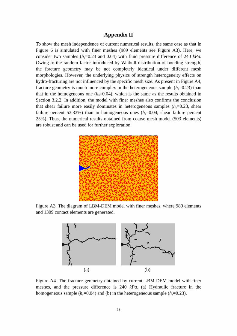
Appendix II To show the mesh independence of current numerical results, the same case as that in Figure 6 is simulated with finer meshes (989 elements see Figure A3). Here, we consider two samples (hs=0.23 and 0.04) with fluid pressure difference of 240 kPa. Owing to the random factor introduced by Weibull distribution of bonding strength, the fracture geometry may be not completely identical under different mesh morphologies. However, the underlying physics of strength heterogeneity effects on hydro-fracturing are not influenced by the specific mesh size. As present in Figure A4, fracture geometry is much more complex in the heterogeneous sample (hs=0.23) than that in the homogeneous one (hs=0.04), which is the same as the results obtained in Section 3.2.2. In addition, the model with finer meshes also confirms the conclusion that shear failure more easily dominates in heterogeneous samples (hs=0.23, shear failure percent 53.33%) than in homogeneous ones (hs=0.04, shear failure percent 25%). Thus, the numerical results obtained from coarse mesh model (503 elements) are robust and can be used for further exploration.

Figure A3. The diagram of LBM-DEM model with finer meshes, where 989 elements and 1309 contact elements are generated.

Figure A4. The fracture geometry obtained by current LBM-DEM model with finer meshes, and the pressure difference is 240 kPa. (a) Hydraulic fracture in the homogeneous sample (hs=0.04) and (b) in the heterogeneous sample (hs=0.23).

(a) (b)

28

Reference

Adachi, A., E. Siebrits, A. Peirce, and J. Desroches (2007), Computer simulation of hydraulic fractures, International Journal of Rock Mechanics and Mining Sciences, 44(5), 739-757.

Al-Busaidi, A., J. F. Hazzard, and R. P. Young (2005), Distinct element modeling of hydraulically fractured Lac du Bonnet granite, Journal of Geophysical Research: Solid Earth, 110, B06302, doi:10.1029/2004jb003297.

Barbati, A. C., J. Desroches, A. Robisson, and G. H. McKinley (2016), Complex Fluids and Hydraulic Fracturing, Annual Review of Chemical and Biomolecular Engineering, 7, 415-453.

Bouma, T., K. L. Nielsen, J. Van Hal, and B. Koutstaal (2001), Root system topology and diameter distribution of species from habitats differing in inundation frequency, Functional Ecology, 15(3), 360-369.

Boutt, D., B. Cook, and J. Williams (2011), A coupled fluid–solid model for problems in geomechanics: application to sand production, International Journal for Numerical and Analytical Methods in Geomechanics, 35(9), 997-1018.

Bruno, M., A. Dorfmann, K. Lao, and C. Honeger (2001), Coupled particle and fluid flow modeling of fracture and slurry injection in weakly consolidated granular media, paper presented at DC Rocks 2001, The 38th US Symposium on Rock Mechanics (USRMS), American Rock Mechanics Association.

Chen, S., and G. D. Doolen (1998), Lattice Boltzmann method for fluid flows, Annual Review of Fluid Mechanics, 30(1), 329-364.

Chen, Y., Q. Cai, Z. Xia, M. Wang, and S. Chen (2013), Momentum-exchange method in lattice Boltzmann simulations of particle-fluid interactions, Physical Review E, 88(1), 013303.

Chen, Y., Q. Kang, Q. Cai, M. Wang, and D. Zhang (2015), Lattice Boltzmann Simulation of Particle Motion in Binary Immiscible Fluids, Communications in Computational Physics, 18(03), 757-786.

Chen, Z., C. Xie, Y. Chen, and M. Wang (2016), Bonding Strength Effects in Hydro-Mechanical Coupling Transport in Granular Porous Media by Pore-Scale Modeling, Computation, 4(1), 15, doi:10.3390/computation4010015.

Chitrala, Y., C. Sondergeld, and C. Rai (2012a), Acoustic emission studies of hydraulic fracture evolution using different fluid viscosities, paper presented at 46th US Rock Mechanics/Geomechanics Symposium, American Rock Mechanics Association.

Chitrala, Y., C. H. Sondergeld, and C. S. Rai (2012b), Microseismic Studies of Hydraulic Fracture Evolution at Different Pumping Rates, paper presented at SPE Americas Unconventional Resources Conference, Society of Petroleum Engineers.

Chong, K. K., O. A. Jaripatke, W. V. Grieser, and A. Passman (2010), A completions roadmap to shale-play development: A review of successful approaches toward shale-play stimulation in the last two decades, paper presented at International Oil and Gas Conference and Exhibition in China, Society of Petroleum Engineers.

Cornet, F., and B. Valette (1984), In situ stress determination from hydraulic injection test data, Journal of Geophysical Research: Solid Earth, 89(B13), 11527-11537.

Cundall, P. A., and O. D. Strack (1979), A discrete numerical model for granular assemblies, Geotechnique, 29(1), 47-65.

Detournay, E. (2016), Mechanics of hydraulic fractures, Annual Review of Fluid Mechanics, 48, 311-339.

Economides, M. J., and K. G. Nolte (2000), Reservoir stimulation, Wiley Chichester.

29

Eshiet, K. I., Y. Sheng, and J. Ye (2013), Microscopic modelling of the hydraulic fracturing process, Environmental Earth Sciences, 68(4), 1169-1186.

Falls, S., R. Young, S. Carlson, and T. Chow (1992), Ultrasonic tomography and acoustic emission in hydraulically fractured Lac du Bonnet grey granite, Journal of Geophysical Research: Solid Earth, 97(B5), 6867-6884.

Fortes, A. F., D. D. Joseph, and T. S. Lundgren (1987), Nonlinear mechanics of fluidization of beds of spherical particles, Journal of Fluid Mechanics, 177, 467-483.

Furtney, J., F. Zhang, and Y. Han (2013), Review of methods and applications for incorporating fluid flow in the Discrete Element Method, paper presented at Proceedings of the 3rd International FLAC/DEM Symposium, Hangzhou, China.

Galindo-Torres, S., D. Pedroso, D. Williams, and L. Li (2012), Breaking processes in three-dimensional bonded granular materials with general shapes, Computer Physics Communications, 183(2), 266-277.

Geertsma, J., and F. De Klerk (1969), A rapid method of predicting width and extent of hydraulically induced fractures, Journal of Petroleum Technology, 21(12), 1571-1581.

Glowinski, R., T. Pan, T. Hesla, D. Joseph, and J. Periaux (2001), A fictitious domain approach to the direct numerical simulation of incompressible viscous flow past moving rigid bodies: application to particulate flow, Journal of Computational Physics, 169(2), 363-426.

Gou, Y., L. Zhou, X. Zhao, Z. Hou, and P. Were (2015), Numerical study on hydraulic fracturing in different types of georeservoirs with consideration of H2M-coupled leak-off effects, Environmental Earth Sciences, 73(10), 6019-6034.

Hazzard, J. F., R. P. Young, and S. J. Oates (2002), Numerical modeling of seismicity induced by fluid injection in a fractured reservoir, paper presented at Mining and Tunnel Innovation and Opportunity, Proceedings of the 5th North American Rock Mechanics Symposium, Toronto, Canada, Citeseer.

Ishida, T. (2001), Acoustic emission monitoring of hydraulic fracturing in laboratory and field, Construction and Building Materials, 15(5), 283-295.

Ishida, T., Q. Chen, and Y. Mizuta (1997), Effect of injected water on hydraulic fracturing deduced from acoustic emission monitoring, Pure and Applied Geophysics, 150, 627-646.

Ishida, T., Q. Chen, Y. Mizuta, and J. C. Roegiers (2004), Influence of fluid viscosity on the hydraulic fracturing mechanism, Journal of Energy Resources Technology, 126(3), 190-200.

Kovalyshen, Y. (2010), Fluid-driven fracture in poroelastic medium, University of Minnesota. Latham, J. P., J. Xiang, M. Belayneh, H. M. Nick, C. F. Tsang, and M. J. Blunt (2013), Modelling

stress-dependent permeability in fractured rock including effects of propagating and bending fractures, International Journal of Rock Mechanics and Mining Sciences, 57, 100-112.

Lisjak, A., O. Mahabadi, B. Tatone, K. Alruwaili, G. Couples, J. Ma, and A. Al-Nakhli (2015), 3D simulation of fluid-pressure-induced fracture nucleation and growth in rock samples, paper presented at 49th US Rock Mechanics/Geomechanics Symposium, American Rock Mechanics Association.

Liu, C., C. S. Tang, B. Shi, and W. B. Suo (2013), Automatic quantification of crack patterns by image processing, Computers & Geosciences, 57, 77-80.

Liu, P., Y. Ju, P. G. Ranjith, Z. Zheng, and J. Chen (2016), Experimental investigation of the effects of heterogeneity and geostress difference on the 3D growth and distribution of hydrofracturing cracks in unconventional reservoir rocks, Journal of Natural Gas Science and Engineering, 35, 541-554.

Ma, G., Q. Wang, X. Yi, and X. Wang (2014), A modified SPH method for dynamic failure simulation of

30

heterogeneous material, Mathematical Problems in Engineering, 2014, 808359. Ma, G., X. Wang, and F. Ren (2011), Numerical simulation of compressive failure of heterogeneous

rock-like materials using SPH method, International Journal of Rock Mechanics and Mining Sciences, 48(3), 353-363.

Mayerhofer, M. J., E. Lolon, N. R. Warpinski, C. L. Cipolla, D. W. Walser, and C. M. Rightmire (2010), What is stimulated reservoir volume?, SPE Production & Operations, 25(01), 89-98.

McClintock, F., and F. Zaverl Jr (1979), An analysis of the mechanics and statistics of brittle crack initiation, International Journal of Fracture, 15(2), 107-118.

Ni, X. D., C. Zhu, and Y. Wang (2015), Hydro-Mechanical Analysis of Hydraulic Fracturing Based on an Improved DEM-CFD Coupling Model at Micro-Level, Journal of Computational and Theoretical Nanoscience, 12(9), 2691-2700.

Nick, H., A. Paluszny, M. Blunt, and S. Matthai (2011), Role of geomechanically grown fractures on dispersive transport in heterogeneous geological formations, Physical Review E, 84(5), 056301.

Noble, D., and J. Torczynski (1998), A lattice-Boltzmann method for partially saturated computational cells, International Journal of Modern Physics C, 9(08), 1189-1201.

Nordgren, R. (1972), Propagation of a vertical hydraulic fracture, Society of Petroleum Engineers Journal, 12(04), 306-314.

Oppelt, A. L., W. Kurth, and D. L. Godbold (2001), Topology, scaling relations and Leonardo's rule in root systems from African tree species, Tree Physiology, 21(2), 117-128.

Qian, Y. H., D. Dhumieres, and P. Lallemand (1992), Lattice BGK model for Navier-Stokes equation, Europhysics Letters, 17(6), 479-484.

Qiu, K., N. Cheng, X. Ke, Y. Liu, L. Wang, Y. Chen, Y. Wang, and P. Xiong (2013), 3D Reservoir Geomechanics Workflow and Its Application to a Tight Gas Reservoir in Western China, paper presented at IPTC 2013: International Petroleum Technology Conference.

Rahman, M., and M. Rahman (2010), A review of hydraulic fracture models and development of an improved pseudo-3D model for stimulating tight oil/gas sand, Energy Sources, Part A: Recovery, Utilization, and Environmental Effects, 32(15), 1416-1436.

Rossi, P., and S. Richer (1987), Numerical modelling of concrete cracking based on a stochastic approach, Materials and Structures, 20(5), 334-337.

Sharma, N., and N. A. Patankar (2005), A fast computation technique for the direct numerical simulation of rigid particulate flows, Journal of Computational Physics, 205(2), 439-457.

Sheng, Y., M. Sousani, D. Ingham, and M. Pourkashanian (2015), Recent Developments in Multiscale and Multiphase Modelling of the Hydraulic Fracturing Process, Mathematical Problems in Engineering, 2015, 729672.

Shimizu, H., S. Murata, and T. Ishida (2011), The distinct element analysis for hydraulic fracturing in hard rock considering fluid viscosity and particle size distribution, International Journal of Rock Mechanics and Mining Sciences, 48(5), 712-727.

Stoeckhert, F., M. Molenda, S. Brenne, and M. Alber (2015), Fracture propagation in sandstone and slate–Laboratory experiments, acoustic emissions and fracture mechanics, Journal of Rock Mechanics and Geotechnical Engineering, 7(3), 237-249.

Strack, O. E., and B. K. Cook (2007), Three‐dimensional immersed boundary conditions for moving solids in the lattice‐Boltzmann method, International Journal for Numerical Methods in Fluids, 55(2), 103-125.

Succi, S. (2001), The lattice Boltzmann equation: for fluid dynamics and beyond, Oxford university

31

press. Talebi, S., and F. H. Cornet (1987), Analysis of the microseismicity induced by a fluid injection in a

granitic rock mass, Geophysical Research Letters, 14(3), 227-230. Tang, C., H. Liu, P. Lee, Y. Tsui, and L. Tham (2000), Numerical studies of the influence of microstructure

on rock failure in uniaxial compression—part I: effect of heterogeneity, International Journal of Rock Mechanics and Mining Sciences, 37(4), 555-569.

Thallak, S., L. Rothenburg, and M. Dusseault (1991), Simulation of multiple hydraulic fractures in a discrete element system, paper presented at The 32nd US Symposium on Rock Mechanics (USRMS), American Rock Mechanics Association.

Veatch Jr, R., and Z. Moschovidis (1986), An overview of recent advances in hydraulic fracturing technology, paper presented at International Meeting on Petroleum Engineering, Society of Petroleum Engineers.

Wang, M., and S. Chen (2007), Electroosmosis in homogeneously charged micro-and nanoscale random porous media, Journal of Colloid and Interface Science, 314(1), 264-273.

Wang, M., J. Wang, N. Pan, and S. Chen (2007), Mesoscopic predictions of the effective thermal conductivity for microscale random porous media, Physical Review E, 75(3), 036702.

Wang, T., W. Zhou, J. Chen, X. Xia, Y. Li, and X. Zhao (2014), Simulation of hydraulic fracturing using particle flow method and application in a coal mine, International Journal of Coal Geology, 121, 1-13.

Wang, Z., X. Jin, X. Wang, L. Sun, and M. Wang (2016), Pore-scale geometry effects on gas permeability in shale, Journal of Natural Gas Science and Engineering, 34, 948-957.

Warpinski, N., and L. Teufel (1987), Influence of geologic discontinuities on hydraulic fracture propagation Journal of Petroleum Technology, 39(02), 209-220.

Yardley, B. W. (1983), Quartz veins and devolatilization during metamorphism, Journal of the Geological Society, 140(4), 657-663.

Yew, C. H., and X. Weng (2014), Mechanics of hydraulic fracturing, Gulf Professional Publishing. Zhang, L., and M. Wang (2015), Modeling of electrokinetic reactive transport in micropore using a

coupled lattice Boltzmann method, Journal of Geophysical Research: Solid Earth, 120(5), 2877-2890. Zhang, X., D. J. Sanderson, and A. J. Barker (2002), Numerical study of fluid flow of deforming

fractured rocks using dual permeability model, Geophysical Journal International, 151(2), 452-468. Zhou, L., and M. Z. Hou (2013), A new numerical 3D-model for simulation of hydraulic fracturing in

consideration of hydro-mechanical coupling effects, International Journal of Rock Mechanics and Mining Sciences, 60, 370-380.

Zhou, L., M. Z. Hou, Y. Gou, and M. Li (2014), Numerical investigation of a low-efficient hydraulic fracturing operation in a tight gas reservoir in the North German Basin, Journal of Petroleum Science and Engineering, 120, 119-129.

32