Population synthesis of cataclysmic variable star: I. A new methodology and initial study on the post common-envelope stage

Astrophys Space Sci (2013) 346:79–87DOI 10.1007/s10509-013-1447-9

O R I G I NA L A RT I C L E

Population synthesis of cataclysmic variable star:I. A new methodology and initial study on the postcommon-envelope stage

P. Irawati · P. Mahasena · D. Herdiwijaya · F.P. Zen

Received: 17 October 2012 / Accepted: 8 April 2013 / Published online: 20 April 2013© Springer Science+Business Media Dordrecht 2013

Abstract We report the results of our population synthesisfor post common-envelope binaries by following the evolu-tion of each system in detail. Our main focus is a compari-son with the white dwarf mass distribution of post common-envelope systems from the Sloan Digital Sky Survey. Weemploy a Monte Carlo method to choose the initial param-eters of the progenitors (primary mass, mass ratio and or-bital period). Then the evolution of the progenitor binarysystem is followed up to the onset of the common-envelopephase, which usually occurs near the tip of the giant branchor asymptotic giant branch. An approximate post-Heliumflash evolution for primary masses ≤2.25M� is included.The binary parameters before and after common-envelopephase are calculated using the energy budget argument. Inthis paper we address the case of αCE = 1.0, which is thecommonly adopted value to calculate the common-envelopeejection. We consider a hydrogen-exhausted core to definethe core mass of the primary (white dwarf mass, MWD) at theonset of common envelope phase. To obtain the present-dayMWD distributions, we assumed a constant star formationrate. The distribution resulting from our population synthe-

P. Irawati (�)National Astronomical Research Institute of Thailand,191 Siriphanich Bldg., Huay Kaew Rd., Suthep, Muang,Chiang Mai 50200, Thailande-mail: [email protected]

P. Irawati · P. Mahasena · D. HerdiwijayaAstronomy Research Group, Faculty of Mathematics andNatural Sciences, Institut Teknologi Bandung, Bandung 40132,Indonesia

F.P. ZenTheoretical Physics Laboratory, THEPI, Faculty of Mathematicsand Natural Sciences, Institut Teknologi Bandung,Bandung 40132, Indonesia

sis shows a double peak profile for MWD, similar to pre-vious population syntheses and recent observational data.Our present synthesis result could not reproduce the loca-tion of the low and high mass peaks from the observations,but shows how a future synthesis can be made to produce anMWD distribution which is closer to observational data.

Keywords Binaries: close, common envelope · Star:evolution, population synthesis · Cataclysmic variables

1 Introduction

A cataclysmic variable (CV) is a binary system in which awhite dwarf (the primary star) is accreting mass from a lowmass, late-type companion through the Lagrangian L1 point.The orbital periods of these systems range from ∼80 min-utes to ∼10 hours, implying that their orbital size is compa-rable to that of the Sun.

The standard scenario from Paczynski (1976) prescribesa common-envelope (CE) phase to form this binary (seealso, e.g. Iben and Livio 1993). In this scenario, a CVevolves from main-sequence progenitor stars, consisting ofa more massive primary star and a low mass secondary ina longer orbit. The primary will follow a single star evo-lution and expands into a red giant star. When the primaryexpands into a red giant star during the first giant branchor the asymptotic giant branch (AGB), it may fill its Rochelobe (provided an appropriate initial size of the orbit) andtriggers an unstable mass transfer. Both the primary and thesecondary stars will move closer as their separation is re-duced during the mass transfer phase, leading up to a CEphase. The secondary star loses its angular momentum dueto frictional effects inside the giant’s envelope. As a result,the secondary spirals in, and, disrupts the outer envelope of

80 Astrophys Space Sci (2013) 346:79–87

the primary, leaving the core of the primary (now a whitedwarf) accompanied by a low mass secondary as a remnant.We refer to the system after CE as a post common-envelopebinary (PCEB).

The PCEB will continue its evolution into a more com-pact binary system. The orbit will shrink due to angu-lar momentum loss via magnetic braking (Verbunt andZwaan 1981) and gravitational radiation (Paczynski andSienkiewicz 1981). Once the secondary star fills its Rochelobe it will start the second mass transfer phase onto thewhite dwarf. This is the phase when the system will be ob-served as CV.

Studies on post-CE binaries, cataclysmic variables andsimilar systems have been done by many authors both the-oretically and observationally. The first few studies (e.g.Paczynski 1976; Ritter 1976; Eggleton 1976) discuss aboutthe formation scenarios and the possible progenitor systemsof CVs. Then through 1980s until recently, there were manyquantitative studies to simulate the distribution of CVs.These works include the initial statistical works by Politano(1988) which later are followed by de Kool (1992), Kolb(1993), and Politano (1996). Those statistical studies havehelped in advancing our comprehension of the formation ofCV systems. Our current understanding on the CV evolu-tion has come from the point of view of the secondary star.Knigge et al. (2011) carried out semi-empirical studies onthe mass transfer and angular momentum loss rates in CVsbased on the mass-radius relationship of the secondary stars.They show that the secondary star is slightly out of thermalequilibrium (bloated) as a response to mass loss, hence themass-radius relationship of the secondary star would serveas a good indicator of the mass transfer rate in CVs.

The population synthesis is a powerful tool to calculatethe present day distribution of any stars, under some as-sumptions. But to obtain results which are able to representthe real distribution one has to evolve hundred thousands,even millions of models. This is the reason why the use ofanalytic approximation or the grid of evolution tracks is veryfavorable. Politano (2004) employs a Jacobian technique tofind the present day distribution of CVs with brown dwarfsecondaries. The Jacobian code implements a complete an-alytical fits to calculate the stellar evolution of the binaries.Shortly after, Willems and Kolb (2004) published a popula-tion synthesis study using the BiSEPS code to investigate theformation of detached white dwarf main-sequence binaries.The BiSEPS code is based on the single star evolution gridfrom Hurley et al. (2000) and the binary evolution algorithmby Hurley et al. (2002). Recent studies by Davis et al. (2008,2010) follow a similar presciption to find the distributions ofWDMS and post-CE binaries.

Nelson (2012) introduces new techniques on the popula-tion synthesis for interacting binaries where the evolution ofsecondary stars are taken into account. The first technique is

done by preparing a fine-grid of initial conditions consists of42,000 evolutionary tracks, which allows them to determinethe progenitor systems and the evolutionary channels of cer-tain binaries. The second method implements a grid interpo-lation of pre-computed evolutionary tracks. This method of-fers a prudent way to carry out population syntheses wherethe computational work is performed to choose the initialconditions, and to do the grid interpolation.

While previous works on the population synthesis ofpost-CE systems described above utilizes grid and analyti-cal fits to compute the evolutionary tracks, we use a differentapproach by evolving each system from the zero age mainsequence (ZAMS) to the CE phase. This direct evolutionmethod will allow us to follow in detail the changes in thestellar structure and the orbital parameters of the systems. Itis clear that such a method requires a long computing time,compared to the population synthesis with a grid of evolu-tionary tracks, but we believe that we will be able to seecertain details which grid method may not provide. One ofthe details is a ‘brief decrease’ in the core mass during theasymptotic giant branch (AGB) phase which contribute tothe high-mass tail in the white dwarf mass distribution (seeSect. 3).

Our main interest in this work is the evolutionary processbefore the CE stage and our work focuses on acquiring thedistribution of the post-CE systems. We consider an enve-lope binding energy presciption (e.g. de Kool 1992; Daviset al. 2010) with ejection efficiency parameter (αCE) to cal-culate the CE phase

αCE ≡ Ebind

�Eorb. (1)

αCE is a dimensionless parameter which determines how ef-ficient the process of the ejection of the envelope is. Theejection takes place efficiently if the difference of the orbitalenergy before and after the CE phase (�Eorb) equals to theenergy needed to expell the envelope of the primary (Ebind).

The value of αCE ranges between 0 < αCE ≤ 1.0. Albeitthis definition higher value where αCE > 1.0 has to be con-sidered for special cases like IK Peg. We will not discuss theoption for αCE > 1.0 as it is beyond the scope of this pa-per. We refer the readers to other works by Nelemans et al.(2000), Nelemans and Tout (2000), Davis et al. (2012) for amore detailed explanation.

αCE plays an important role in the close binary evolu-tion therefore the quest to find the exact value of αCE is in-escapable. However, despite a lot of effort in modelling andstudying the CE evolution, the physical nature of αCE re-mains uncertain. We note that the αCE we use in this work(αCE = 1.0) is the commonly adopted value (e.g. de Kooland Ritter 1993; Howell et al. 2001; Willems and Kolb 2004)and we use it simply as a test case. It is our goal to pursuethe investigation of different αCE values in future works.

Astrophys Space Sci (2013) 346:79–87 81

We describe our computational method and assumptionsin Sect. 2. The results of our synthesis, together with theother models (Howell et al. 2001; Davis et al. 2010) and theobservational data as comparison, are presented in Sect. 3.We realize that our synthesis results represent the distribu-tion without any bias while the observational data is verysubjected to observational selection effects. The discussionand conclusion will be given in Sect. 4.

2 Computational method

We use the STARS evolution code (Eggleton 1971, 1972;Eggleton et al. 1973) which has been updated and de-veloped during the past four decades (Han et al. 1994;Pols et al. 1995; Nelson and Eggleton 2001). The code si-multaneously solves the stellar structure and composition,using a self-adaptive, non-Lagrangian meshpoint distribu-tion. The angular momentum loss through gravitational ra-diation and magnetic braking process have been included toreproduce the close binary evolution, especially in the abilityto reproduce the 2–3 hr period gap in CVs. The mass transferprocess is assumed to proceed in a conservative way and thebinary will always be in a circular orbit with synchronousrotation.

We use the single star evolution mode of the STARScode. In this mode, the code will evolve only the primarystar in a binary system while the secondary star acts as pointof mass to help to calculate the orbital parameters of thesystem (e.g. period, Roche lobe radii of both components,mass transfer rate, angular momentum loss from the system,etc.). A typical running time for one evolution from zero agemain sequence (ZAMS) to the tip of first giant branch, orasymptotic giant branch, is ten minutes on a PC with triplecore CPU, 2.0 GHz. We are aware that the recent version(e.g. van der Sluys et al. 2006) offers a more sophisticatedchoice (the ‘TWIN’ mode) to evolve both the primary andthe secondary stars simultaneously but certainly with longercomputing time. Due to this reason and also because of ourlimited computing facility we choose the single star modefor our work to obtain a larger number of models.

We develop a population synthesis code to simulate thepresent-day distribution of PCEBs. Our code is designed toevolve systems which will experience the CE phase. TheSTARS code needs three main inputs to evolve the stellarmodel, they are the primary mass (M1), mass ratio (q), andthe orbital period (Porb) of the initial system. We employthe Monte Carlo method to choose those three inputs andimpose some constraints so that the progenitors will likelybecome a post-CE binary.

2.1 Initial model and eligibility criteria

The M1 distribution of the progenitors should follow the Ini-tial Mass Function (IMF) from Miller and Scalo (1979). We

use the IMF formulation in the approximation of Eggletonet al. (1989)

M1 = 0.19X

(1 − X)0.75 + 0.032(1 − X)0.25(2)

where X is a random number distributed between 0 and 1.We choose the range of M1 to be 1.0 M� < M1 < 9.0 M�.The lower limit is the lowest mass which can evolve intoa CE binary within the age of Galactic disc while the up-per limit is chosen to avoid neutron star formation in a corecollapse supernova.

Following Howell et al. (2001), the mass ratio is cal-culated from the probability distribution function f (q) =54 q1/4 where q ≡ M2/M1 (Abt and Levy 1978). Howellet al. (2001) found that the results of their population synthe-sis are not especially sensitive to the choice of f (q). How-ever, Nelson et al. (2004) show that f (q) can moderatelyaffect the number of Galactic novae based on their synthesisresults. In this work we choose only one function of f (q)

with the value of q generated should meet the limitation ofq < 0.4. The constraint for q is chosen (empirically, aftersome preliminary parameter studies, including q) to guaran-tee the occurrence of unstable mass transfer which will leadto the CE phase.

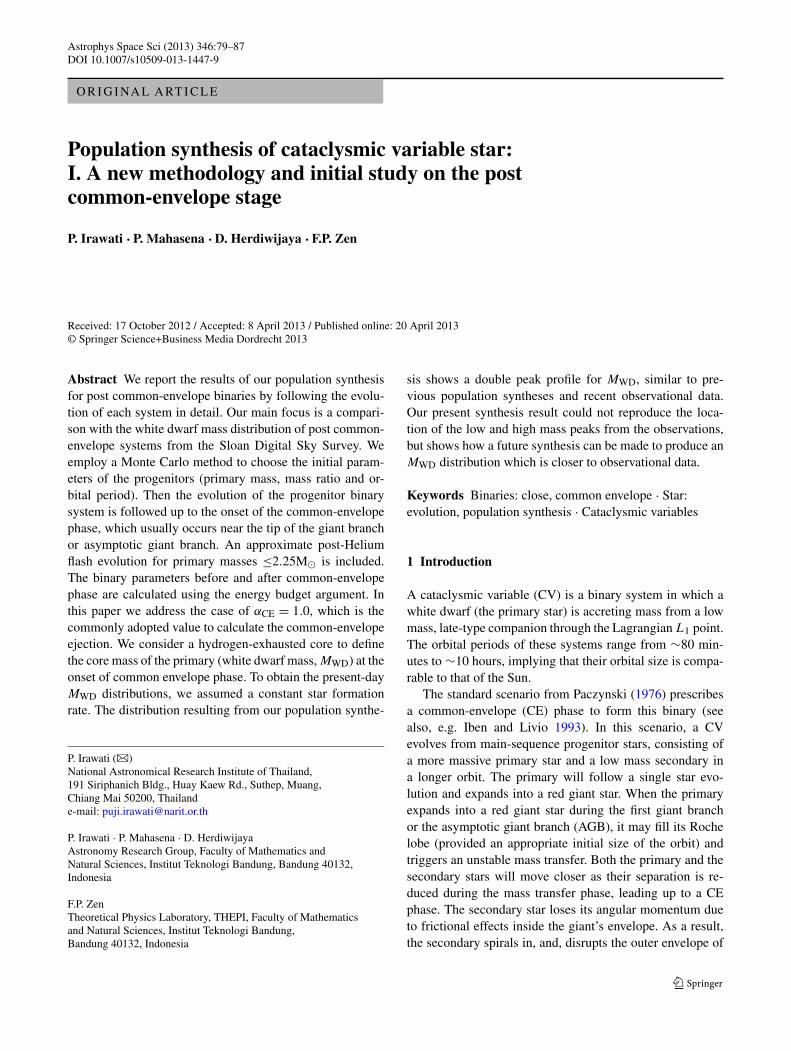
In our simulation, the start of an unstable mass transfer(hence, common envelope phase) is defined numerically bya critical value of dPorb/dt (a negative value) below whichthe code cannot follow orbital parameter changes (dt be-comes unrealistically small). We find that, in most cases, theunstable mass transfer occurs as Case B or Case C. Interest-ingly, the unstable mass transfer which will lead to a post-CE binary always starts on the tip of the giant branch or theAGB (Fig. 1). Exclusively this means RL,1/R1 > 40 at thebeginning of the evolution. Otherwise, RL,2/R2 < 1 (for thesecondary), after the CE phase.

In our calculation we assume that all stars are in binariesand we choose the initial orbital period (Porb) from a uni-form distribution of log(P ) over the period range of 1 dayto 106 years (see, e.g., Howell et al. 2001).

As part of our initial study, we investigate the role of stel-lar wind and metallicity in the white dwarf mass (MWD)distribution of PCEB. First, we perform population synthe-ses for different values of stellar wind parameter (ηR) withsmaller number of samples. We use the stellar wind modelfrom Reimers (1975) with mass loss rate (M) presciption

M = −4 × 10−13ηR

L

gR

(M� yr−1) (3)

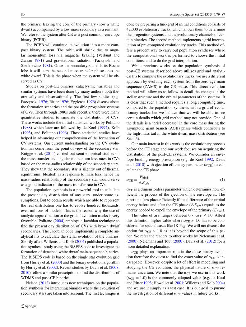
where g, L and R are the surface gravity, the luminosity, andthe radius of the star, respectively. ηR is a constant whichdefines the amount of the mass loss by stellar wind in theSTARS code. In this study we use three values of ηR , whichare 0.0, 0.3 and 0.5.

82 Astrophys Space Sci (2013) 346:79–87

Fig. 1 The location of PCEBs from our population synthesis plottedover the evolution tracks of single star with masses 1 − 8M�. All ofthe PCEBs in our result start their mass transfer phase at the tip of thegiant branch or AGB. The crosses (+) mark the systems which undergothe horizontal branch evolution. The filled-circles (•) are the systemswhich finish the evolution without going through the horizontal branch

Fig. 2 MWD distribution for each stellar wind parameter: ηR = 0.0(black), ηR = 0.3 (red), ηR = 0.5 (green)

The dependency of the MWD distribution to the stellarwind parameter is shown in Figs. 2 and 3. We find simi-lar result as in other works (Politano 1996) where the MWD

distribution consists of two groups. The lower mass group isthe systems with He WD and the higher mass group is thesystems with CO WD. Increasing value of ηR will reducethe relative number of PCEBs with CO WDs. The gap in thedistribution of MWD is due to the core growth process dur-ing the giant branch and the asymptotic giant branch evolu-tion (Politano 1996). For the present work we choose to useηR = 0.3 as a test case. We plan to elaborate on the choicesof stellar wind in our future synthesis work.

In the second initial study, we inspect the dependency ofthe MWD distribution to the metallicity (Z) by using twovalues of metallicity, 0.02 and 0.002. We perform popula-tion syntheses for the two values of Z in a similar manneras before, using smaller number of samples. We calculatethe hydrogen and helium abundances as functions of metal-licity: X = 0.76 − 3.0Z and Y = 0.24 + 2.0Z (Pols et al.1998).

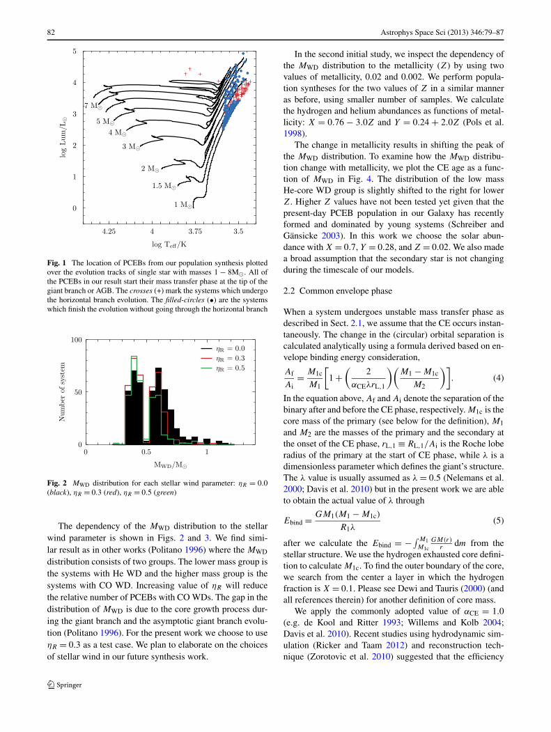
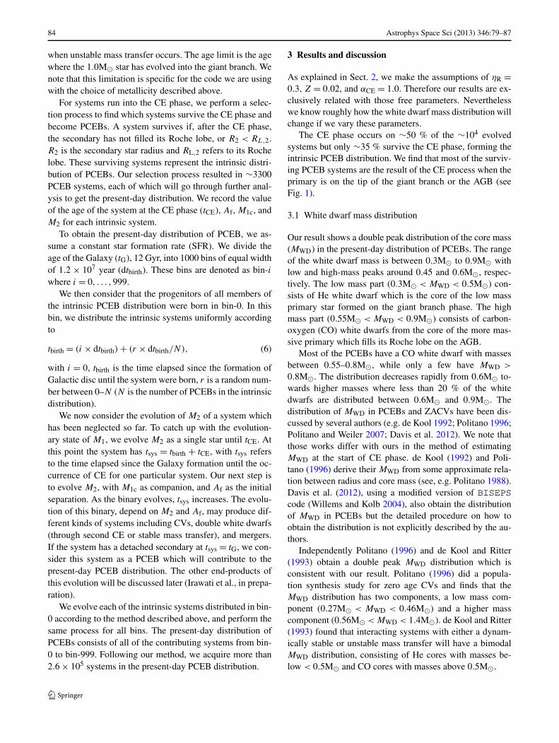
The change in metallicity results in shifting the peak ofthe MWD distribution. To examine how the MWD distribu-tion change with metallicity, we plot the CE age as a func-tion of MWD in Fig. 4. The distribution of the low massHe-core WD group is slightly shifted to the right for lowerZ. Higher Z values have not been tested yet given that thepresent-day PCEB population in our Galaxy has recentlyformed and dominated by young systems (Schreiber andGänsicke 2003). In this work we choose the solar abun-dance with X = 0.7, Y = 0.28, and Z = 0.02. We also madea broad assumption that the secondary star is not changingduring the timescale of our models.

2.2 Common envelope phase

When a system undergoes unstable mass transfer phase asdescribed in Sect. 2.1, we assume that the CE occurs instan-taneously. The change in the (circular) orbital separation iscalculated analytically using a formula derived based on en-velope binding energy consideration,

Af

Ai= M1c

M1

[1 +

(2

αCEλrL,1

)(M1 − M1c

M2

)]. (4)

In the equation above, Af and Ai denote the separation of thebinary after and before the CE phase, respectively. M1c is thecore mass of the primary (see below for the definition), M1

and M2 are the masses of the primary and the secondary atthe onset of the CE phase, rL,1 ≡ RL,1/Ai is the Roche loberadius of the primary at the start of CE phase, while λ is adimensionless parameter which defines the giant’s structure.The λ value is usually assumed as λ = 0.5 (Nelemans et al.2000; Davis et al. 2010) but in the present work we are ableto obtain the actual value of λ through

Ebind = GM1(M1 − M1c)

R1λ(5)

after we calculate the Ebind = − ∫ M1M1c

GM(r)r

dm from thestellar structure. We use the hydrogen exhausted core defini-tion to calculate M1c. To find the outer boundary of the core,we search from the center a layer in which the hydrogenfraction is X = 0.1. Please see Dewi and Tauris (2000) (andall references therein) for another definition of core mass.

We apply the commonly adopted value of αCE = 1.0(e.g. de Kool and Ritter 1993; Willems and Kolb 2004;Davis et al. 2010). Recent studies using hydrodynamic sim-ulation (Ricker and Taam 2012) and reconstruction tech-nique (Zorotovic et al. 2010) suggested that the efficiency

Astrophys Space Sci (2013) 346:79–87 83

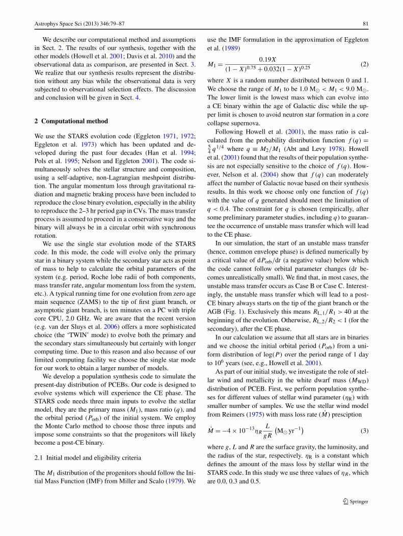
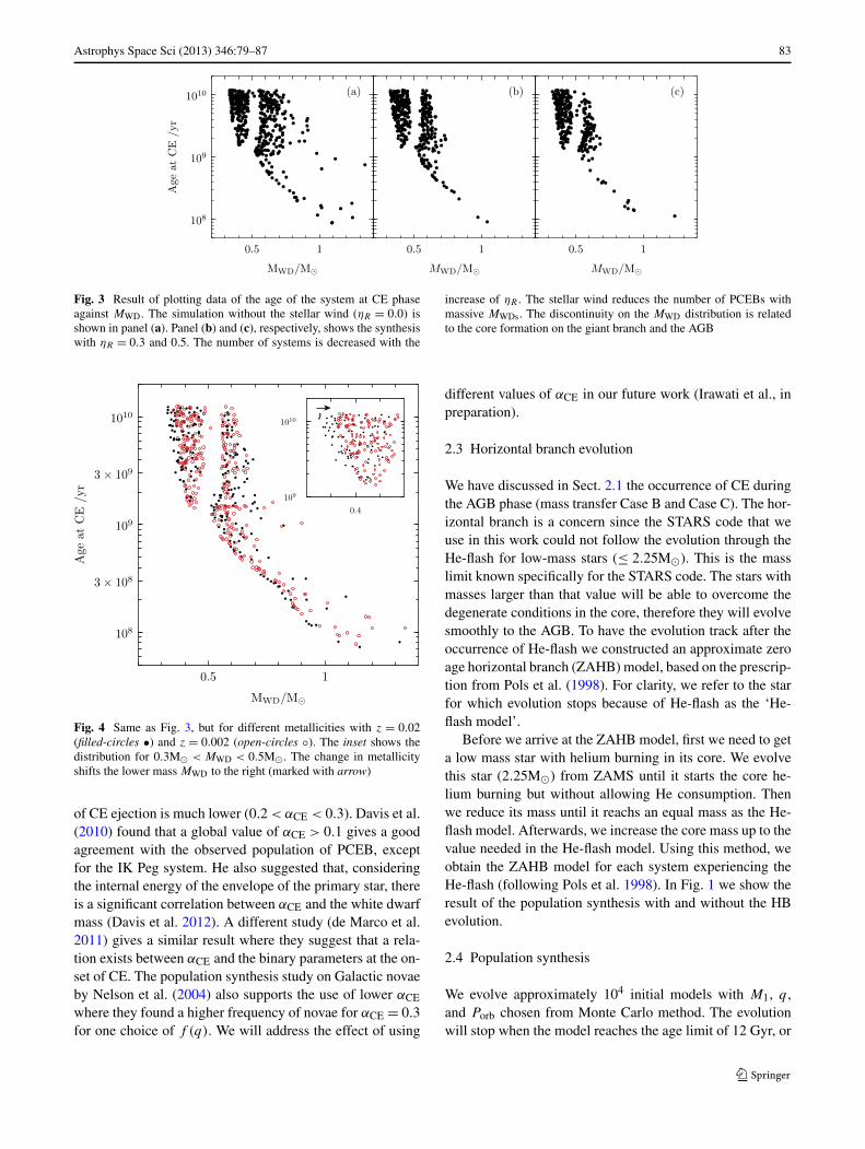
Fig. 3 Result of plotting data of the age of the system at CE phaseagainst MWD. The simulation without the stellar wind (ηR = 0.0) isshown in panel (a). Panel (b) and (c), respectively, shows the synthesiswith ηR = 0.3 and 0.5. The number of systems is decreased with the

increase of ηR . The stellar wind reduces the number of PCEBs withmassive MWDs. The discontinuity on the MWD distribution is relatedto the core formation on the giant branch and the AGB

Fig. 4 Same as Fig. 3, but for different metallicities with z = 0.02(filled-circles •) and z = 0.002 (open-circles ◦). The inset shows thedistribution for 0.3M� < MWD < 0.5M�. The change in metallicityshifts the lower mass MWD to the right (marked with arrow)

of CE ejection is much lower (0.2 < αCE < 0.3). Davis et al.(2010) found that a global value of αCE > 0.1 gives a goodagreement with the observed population of PCEB, exceptfor the IK Peg system. He also suggested that, consideringthe internal energy of the envelope of the primary star, thereis a significant correlation between αCE and the white dwarfmass (Davis et al. 2012). A different study (de Marco et al.2011) gives a similar result where they suggest that a rela-tion exists between αCE and the binary parameters at the on-set of CE. The population synthesis study on Galactic novaeby Nelson et al. (2004) also supports the use of lower αCE

where they found a higher frequency of novae for αCE = 0.3for one choice of f (q). We will address the effect of using

different values of αCE in our future work (Irawati et al., inpreparation).

2.3 Horizontal branch evolution

We have discussed in Sect. 2.1 the occurrence of CE duringthe AGB phase (mass transfer Case B and Case C). The hor-izontal branch is a concern since the STARS code that weuse in this work could not follow the evolution through theHe-flash for low-mass stars (≤ 2.25M�). This is the masslimit known specifically for the STARS code. The stars withmasses larger than that value will be able to overcome thedegenerate conditions in the core, therefore they will evolvesmoothly to the AGB. To have the evolution track after theoccurrence of He-flash we constructed an approximate zeroage horizontal branch (ZAHB) model, based on the prescrip-tion from Pols et al. (1998). For clarity, we refer to the starfor which evolution stops because of He-flash as the ‘He-flash model’.

Before we arrive at the ZAHB model, first we need to geta low mass star with helium burning in its core. We evolvethis star (2.25M�) from ZAMS until it starts the core he-lium burning but without allowing He consumption. Thenwe reduce its mass until it reachs an equal mass as the He-flash model. Afterwards, we increase the core mass up to thevalue needed in the He-flash model. Using this method, weobtain the ZAHB model for each system experiencing theHe-flash (following Pols et al. 1998). In Fig. 1 we show theresult of the population synthesis with and without the HBevolution.

2.4 Population synthesis

We evolve approximately 104 initial models with M1, q ,and Porb chosen from Monte Carlo method. The evolutionwill stop when the model reaches the age limit of 12 Gyr, or

84 Astrophys Space Sci (2013) 346:79–87

when unstable mass transfer occurs. The age limit is the agewhere the 1.0M� star has evolved into the giant branch. Wenote that this limitation is specific for the code we are usingwith the choice of metallicity described above.

For systems run into the CE phase, we perform a selec-tion process to find which systems survive the CE phase andbecome PCEBs. A system survives if, after the CE phase,the secondary has not filled its Roche lobe, or R2 < RL,2.R2 is the secondary star radius and RL,2 refers to its Rochelobe. These surviving systems represent the intrinsic distri-bution of PCEBs. Our selection process resulted in ∼3300PCEB systems, each of which will go through further anal-ysis to get the present-day distribution. We record the valueof the age of the system at the CE phase (tCE), Af, M1c, andM2 for each intrinsic system.

To obtain the present-day distribution of PCEB, we as-sume a constant star formation rate (SFR). We divide theage of the Galaxy (tG), 12 Gyr, into 1000 bins of equal widthof 1.2 × 107 year (dtbirth). These bins are denoted as bin-iwhere i = 0, . . . ,999.

We then consider that the progenitors of all members ofthe intrinsic PCEB distribution were born in bin-0. In thisbin, we distribute the intrinsic systems uniformly accordingto

tbirth = (i × dtbirth) + (r × dtbirth/N), (6)

with i = 0, tbirth is the time elapsed since the formation ofGalactic disc until the system were born, r is a random num-ber between 0–N (N is the number of PCEBs in the intrinsicdistribution).

We now consider the evolution of M2 of a system whichhas been neglected so far. To catch up with the evolution-ary state of M1, we evolve M2 as a single star until tCE. Atthis point the system has tsys = tbirth + tCE, with tsys refersto the time elapsed since the Galaxy formation until the oc-currence of CE for one particular system. Our next step isto evolve M2, with M1c as companion, and Af as the initialseparation. As the binary evolves, tsys increases. The evolu-tion of this binary, depend on M2 and Af, may produce dif-ferent kinds of systems including CVs, double white dwarfs(through second CE or stable mass transfer), and mergers.If the system has a detached secondary at tsys = tG, we con-sider this system as a PCEB which will contribute to thepresent-day PCEB distribution. The other end-products ofthis evolution will be discussed later (Irawati et al., in prepa-ration).

We evolve each of the intrinsic systems distributed in bin-0 according to the method described above, and perform thesame process for all bins. The present-day distribution ofPCEBs consists of all of the contributing systems from bin-0 to bin-999. Following our method, we acquire more than2.6 × 105 systems in the present-day PCEB distribution.

3 Results and discussion

As explained in Sect. 2, we make the assumptions of ηR =0.3, Z = 0.02, and αCE = 1.0. Therefore our results are ex-clusively related with those free parameters. Neverthelesswe know roughly how the white dwarf mass distribution willchange if we vary these parameters.

The CE phase occurs on ∼50 % of the ∼104 evolvedsystems but only ∼35 % survive the CE phase, forming theintrinsic PCEB distribution. We find that most of the surviv-ing PCEB systems are the result of the CE process when theprimary is on the tip of the giant branch or the AGB (seeFig. 1).

3.1 White dwarf mass distribution

Our result shows a double peak distribution of the core mass(MWD) in the present-day distribution of PCEBs. The rangeof the white dwarf mass is between 0.3M� to 0.9M� withlow and high-mass peaks around 0.45 and 0.6M�, respec-tively. The low mass part (0.3M� < MWD < 0.5M�) con-sists of He white dwarf which is the core of the low massprimary star formed on the giant branch phase. The highmass part (0.55M� < MWD < 0.9M�) consists of carbon-oxygen (CO) white dwarfs from the core of the more mas-sive primary which fills its Roche lobe on the AGB.

Most of the PCEBs have a CO white dwarf with massesbetween 0.55–0.8M�, while only a few have MWD >

0.8M�. The distribution decreases rapidly from 0.6M� to-wards higher masses where less than 20 % of the whitedwarfs are distributed between 0.6M� and 0.9M�. Thedistribution of MWD in PCEBs and ZACVs have been dis-cussed by several authors (e.g. de Kool 1992; Politano 1996;Politano and Weiler 2007; Davis et al. 2012). We note thatthose works differ with ours in the method of estimatingMWD at the start of CE phase. de Kool (1992) and Poli-tano (1996) derive their MWD from some approximate rela-tion between radius and core mass (see, e.g. Politano 1988).Davis et al. (2012), using a modified version of BISEPScode (Willems and Kolb 2004), also obtain the distributionof MWD in PCEBs but the detailed procedure on how toobtain the distribution is not explicitly described by the au-thors.

Independently Politano (1996) and de Kool and Ritter(1993) obtain a double peak MWD distribution which isconsistent with our result. Politano (1996) did a popula-tion synthesis study for zero age CVs and finds that theMWD distribution has two components, a low mass com-ponent (0.27M� < MWD < 0.46M�) and a higher masscomponent (0.56M� < MWD < 1.4M�). de Kool and Ritter(1993) found that interacting systems with either a dynam-ically stable or unstable mass transfer will have a bimodalMWD distribution, consisting of He cores with masses be-low < 0.5M� and CO cores with masses above 0.5M�.

Astrophys Space Sci (2013) 346:79–87 85

From the observational side, the number of newly foundPCEBs is increasing rapidly with the help of various skysurvey projects, such as Palomar-Green survey (Green et al.1986), SDSS (Abazajian et al. 2009), and Catalina RealTime Survey (Drake et al. 2009). An extensive analysisfor PCEBs from SDSS has been performed by Rebassa-Mansergas et al. (2010, 2012). These data provide a strongconstraint on the MWD distribution from any population syn-thesis. A possible case can be seen in Fig. 6. The SDSS datareveals a small peak on 0.8M� which is not seen in previouspopulation syntheses mentioned above.

To compare our model with the observed sample, weuse the PCEBs in the SDSS DR6 published by Rebassa-Mansergas et al. (2011). Apart from the big discrepancyin the number of PCEB systems, we are aware that thereare problems of observational selection effects which weneed to address before comparing our result directly withthe observational data. Nevertheless, we hope that the ob-servational data could provide some constraints to verify ourinitial assumptions for the population synthesis. The SDSSdata is known to be affected by the intrinsic selection ef-fects from SDSS survey, which cause bias in the probabilityof finding systems with late-type secondaries, as mentionedby the authors. The detection technique to find PCEBs andCVs in a large sky survey, such as Palomar-Green surveyor SDSS, is exploiting the fact that most CVs are bright inthe blue region due to the brightness of the white dwarf.This method has a tendency to recognize more easily thesystems with late-type secondaries (M3–M5) while systemswith early type secondaries are excluded unintentionally be-cause the light of the secondary dominates over the whitedwarf.

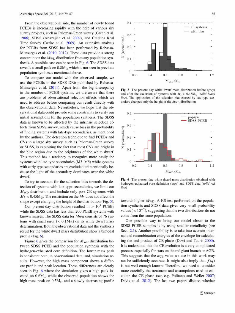
To try to account for the selection bias towards the de-tection of systems with late-type secondaries, we limit ourMWD distribution and include only post-CE systems withM2 < 0.45M�. The restriction on the M2 does not affect theshape except changing the height of the distribution (Fig. 5).

Our present-day distribution resulted in > 105 PCEBswhile the SDSS data has less than 200 PCEB systems withknown masses. The SDSS data for MWD consists of 76 sys-tems with small error (< 0.1M�) on its white dwarf massdetermination. Both the observational data and the synthesisresult for the white dwarf mass distribution show a bimodalprofile (Fig. 6).

Figure 6 gives the comparison for MWD distribution be-tween SDSS PCEB and the population synthesis with thehydrogen-exhausted core definition. The lower mass peakis consistent both, in observational data, and, simulation re-sults. However, the high mass component shows a differ-ent profile and peak location. These differences are clearlyseen in Fig. 6 where the simulation gives a high peak lo-cated on 0.6M� while the observed population shows thehigh mass peak on 0.5M� and a slowly decreasing profile

Fig. 5 The present-day white dwarf mass distribution before (grey)and after the exclusion of systems with M2 > 0.45M� (solid blackline). The application of the selection bias caused by late-type sec-ondary changes only the height of the MWD distribution

Fig. 6 The present-day white dwarf mass distribution obtained withhydrogen-exhausted core definition (grey) and SDSS data (solid redline)

towards higher MWD. A KS test performed on the popula-tion synthesis and SDSS data gives very small probabilityvalues (< 10−7), suggesting that the two distributions do notcome from the same population.

One possible way to bring our model closer to theSDSS PCEB samples is by using smaller metallicity (seeSect. 2.1). Another possibility is to take into account inter-nal and recombination energies of the envelope for calculat-ing the end-product of CE phase (Dewi and Tauris 2000).It is understood that the CE evolution is a very complicatedprocess, especially for stars on the red giant branch or AGB.This suggests that the αCE value we use in this work maynot be sufficiently accurate. It might also imply that f (q)

is not well-enough known. Therefore, we need to considermore carefully the treatment and assumptions used to cal-culate the CE phase (see e.g. Politano and Weiler 2007;Davis et al. 2012). The last two papers discuss whether

86 Astrophys Space Sci (2013) 346:79–87

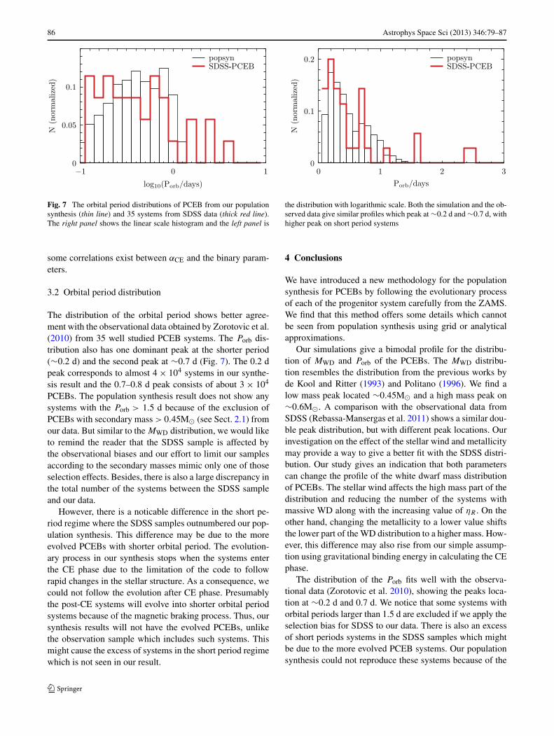
Fig. 7 The orbital period distributions of PCEB from our populationsynthesis (thin line) and 35 systems from SDSS data (thick red line).The right panel shows the linear scale histogram and the left panel is

the distribution with logarithmic scale. Both the simulation and the ob-served data give similar profiles which peak at ∼0.2 d and ∼0.7 d, withhigher peak on short period systems

some correlations exist between αCE and the binary param-eters.

3.2 Orbital period distribution

The distribution of the orbital period shows better agree-ment with the observational data obtained by Zorotovic et al.(2010) from 35 well studied PCEB systems. The Porb dis-tribution also has one dominant peak at the shorter period(∼0.2 d) and the second peak at ∼0.7 d (Fig. 7). The 0.2 dpeak corresponds to almost 4 × 104 systems in our synthe-sis result and the 0.7–0.8 d peak consists of about 3 × 104

PCEBs. The population synthesis result does not show anysystems with the Porb > 1.5 d because of the exclusion ofPCEBs with secondary mass > 0.45M� (see Sect. 2.1) fromour data. But similar to the MWD distribution, we would liketo remind the reader that the SDSS sample is affected bythe observational biases and our effort to limit our samplesaccording to the secondary masses mimic only one of thoseselection effects. Besides, there is also a large discrepancy inthe total number of the systems between the SDSS sampleand our data.

However, there is a noticable difference in the short pe-riod regime where the SDSS samples outnumbered our pop-ulation synthesis. This difference may be due to the moreevolved PCEBs with shorter orbital period. The evolution-ary process in our synthesis stops when the systems enterthe CE phase due to the limitation of the code to followrapid changes in the stellar structure. As a consequence, wecould not follow the evolution after CE phase. Presumablythe post-CE systems will evolve into shorter orbital periodsystems because of the magnetic braking process. Thus, oursynthesis results will not have the evolved PCEBs, unlikethe observation sample which includes such systems. Thismight cause the excess of systems in the short period regimewhich is not seen in our result.

4 Conclusions

We have introduced a new methodology for the populationsynthesis for PCEBs by following the evolutionary processof each of the progenitor system carefully from the ZAMS.We find that this method offers some details which cannotbe seen from population synthesis using grid or analyticalapproximations.

Our simulations give a bimodal profile for the distribu-tion of MWD and Porb of the PCEBs. The MWD distribu-tion resembles the distribution from the previous works byde Kool and Ritter (1993) and Politano (1996). We find alow mass peak located ∼0.45M� and a high mass peak on∼0.6M�. A comparison with the observational data fromSDSS (Rebassa-Mansergas et al. 2011) shows a similar dou-ble peak distribution, but with different peak locations. Ourinvestigation on the effect of the stellar wind and metallicitymay provide a way to give a better fit with the SDSS distri-bution. Our study gives an indication that both parameterscan change the profile of the white dwarf mass distributionof PCEBs. The stellar wind affects the high mass part of thedistribution and reducing the number of the systems withmassive WD along with the increasing value of ηR . On theother hand, changing the metallicity to a lower value shiftsthe lower part of the WD distribution to a higher mass. How-ever, this difference may also rise from our simple assump-tion using gravitational binding energy in calculating the CEphase.

The distribution of the Porb fits well with the observa-tional data (Zorotovic et al. 2010), showing the peaks loca-tion at ∼0.2 d and 0.7 d. We notice that some systems withorbital periods larger than 1.5 d are excluded if we apply theselection bias for SDSS to our data. There is also an excessof short periods systems in the SDSS samples which mightbe due to the more evolved PCEB systems. Our populationsynthesis could not reproduce these systems because of the

Astrophys Space Sci (2013) 346:79–87 87

technical limitation in following the evolution of binaries be-yond the CE phase.

Acknowledgements This work is supported by ITB research grantsyear 2008–2011. The authors would like to thank the referee for theconstructive comments which helped to improve the quality and thepresentation of this paper.

References

Abazajian, K.N., et al.: Astrophys. J. Suppl. Ser. 182, 543 (2009)Abt, H.A., Levy, S.G.: Astrophys. J. Suppl. Ser. 36, 241 (1978)Davis, P.J., Kolb, U., Willems, B., Gänsicke, B.T.: Mon. Not. R. As-

tron. Soc. 389, 1563 (2008)Davis, P.J., Kolb, U., Willems, B.: Mon. Not. R. Astron. Soc. 403, 179

(2010)Davis, P.J., Kolb, U., Knigge, C.: Mon. Not. R. Astron. Soc. 419, 287

(2012)de Kool, M.: Astron. Astrophys. 261, 188 (1992)de Kool, M., Ritter, H.: Astron. Astrophys. 267, 397 (1993)de Marco, O., Passy, J.C., Moe, M., Herwig, F., Low, M.-M., Paxton,

B.: Mon. Not. R. Astron. Soc. 411, 2277 (2011)Dewi, J.D.M., Tauris, T.M.: Astron. Astrophys. 360, 1043 (2000)Drake, A.J., et al.: Astrophys. J. 696, 870 (2009)Eggleton, P.P.: Mon. Not. R. Astron. Soc. 151, 351 (1971)Eggleton, P.P.: Mon. Not. R. Astron. Soc. 156, 361 (1972)Eggleton, P.P.: In: Eggleton, P.P., Mitton, S., Whelan, J. (eds.) Pro-

ceeding of the International Astronomical Union Symposium, p.75 (1976)

Eggleton, P.P., Faulkner, J., Flannery, B.P.: Astron. Astrophys. 23, 325(1973)

Eggleton, P.P., Fitchett, M.J., Tout, C.A.: Astrophys. J. 347, 998 (1989)Green, R.F., Schmidt, M., Liebert, J.: Astrophys. J. Suppl. Ser. 61, 305

(1986)Han, Z., Podsiadlowski, P., Eggleton, P.P.: Mon. Not. R. Astron. Soc.

270, 121 (1994)Howell, S.B., Nelson, L.A., Rappaport, S.: Astrophys. J. 550, 897

(2001)Hurley, J.R., Pols, O.R., Tout, C.A.: Mon. Not. R. Astron. Soc. 315,

543 (2000)

Hurley, J.R., Tout, C.A., Pols, O.R.: Mon. Not. R. Astron. Soc. 329,897 (2002)

Iben, I. Jr., Livio, M.: Publ. Astron. Soc. Pac. 105, 1373 (1993)Knigge, C., Baraffe, I., Patterson, J.: Astrophys. J. Suppl. Ser. 194, 28

(2011)Kolb, U.: Astron. Astrophys. 271, 149 (1993)Miller, G.E., Scalo, J.M.: Astrophys. J. Suppl. Ser. 41, 513 (1979)Nelemans, G., Tout, C.A.: Mon. Not. R. Astron. Soc. 356, 753 (2000)Nelemans, G., Verbunt, F., Yungelson, L.R., Portegies Zwart, S.F.: As-

tron. Astrophys. 360, 1011 (2000)Nelson, L.: J. Phys. Conf. Ser. 341, 012008 (2012)Nelson, C.A., Eggleton, P.P.: Astrophys. J. 552, 664 (2001)Nelson, L.A., MacCannell, K.A., Dubeau, E.: Astrophys. J. 602, 938

(2004)Paczynski, B.: Symp. - Int. Astron. Union 73, 75 (1976)Paczynski, B., Sienkiewicz, R.: Astrophys. J. 248, 27 (1981)Politano, M.: Ph.D. thesis, Univ. of Illinois (1988)Politano, M.: Astrophys. J. 465, 338 (1996)Politano, M.: Astrophys. J. 604, 817 (2004)Politano, M., Weiler, K.P.: Astrophys. J. 665, 663 (2007)Pols, O.R., Tout, C.A., Eggleton, P.P., Han, Z.: Mon. Not. R. Astron.

Soc. 274, 964 (1995)Pols, O.R., Schröder, K.P., Hurley, J.R., Tout, C.A., Eggleton, P.P.:

Mon. Not. R. Astron. Soc. 298, 525 (1998)Rebassa-Mansergas, A., Gänsicke, B.T., Schreiber, M.R., Koester, D.,

Rodríguez-Gil, P.: Mon. Not. R. Astron. Soc. 402, 620 (2010)Rebassa-Mansergas, A., Nebot Gomez-Moran, A., Schreiber, M.R.,

Girven, J., Gänsicke, B.T.: Mon. Not. R. Astron. Soc. 413, 1121(2011)

Rebassa-Mansergas, A., Nebot Gomez-Moran, A., Schreiber, M.R.,Gänsicke, B.T., Schwope, A., Gallardo, J., Koester, D.: Mon. Not.R. Astron. Soc. 419, 806 (2012)

Reimers, D.: Mem. Soc. R. Sci. Liege 8, 369 (1975)Ricker, P.M., Taam, R.E.: Astrophys. J. 746, 74 (2012)Ritter, H.: Mon. Not. R. Astron. Soc. 175, 279 (1976)Schreiber, M.R., Gänsicke, B.T.: Astron. Astrophys. 406, 305 (2003)van der Sluys, M., Verbunt, F., Pols, O.R.: Astron. Astrophys. 460, 209

(2006)Verbunt, F., Zwaan, C.: Astrophys. J. 100, 7 (1981)Willems, B., Kolb, U.: Astron. Astrophys. 419, 1057 (2004)Zorotovic, M., Schreiber, M.R., Gänsicke, B.T., Nebot Gomez-Moran,

A.: Astron. Astrophys. 520, A86 (2010)