Computational Modelling and Prediction of Protease Specificity by Sarah E. Boyd, BSc(ScScholProg) BSc(Hons) Thesis Submitted by Sarah E. Boyd for fulfillment of the Requirements for the Degree of Doctor of Philosophy (0190) Supervisor: Dr. Maria Garcia de la Banda Associate Supervisors: Assoc. Prof. Robert N. Pike and Dr. James C. Whisstock School of Computer Science and Software Engineering Monash University June, 2005

Welcome message from author
This document is posted to help you gain knowledge. Please leave a comment to let me know what you think about it! Share it to your friends and learn new things together.
Transcript

Computational Modelling and Prediction of Protease
Specificity
by
Sarah E. Boyd, BSc(ScScholProg) BSc(Hons)
Thesis
Submitted by Sarah E. Boyd
for fulfillment of the Requirements for the Degree of
Doctor of Philosophy (0190)
Supervisor: Dr. Maria Garcia de la Banda
Associate Supervisors: Assoc. Prof. Robert N. Pike
and Dr. James C. Whisstock
School of Computer Science and Software Engineering
Monash University
June, 2005

c© Copyright
by
Sarah E. Boyd
2005

For Jude
iii
Contents
List of Tables . . . . . . . . . . . . . . . . . . . . . . . . . . . . . . . . . . . . . . vii
List of Figures . . . . . . . . . . . . . . . . . . . . . . . . . . . . . . . . . . . . . viii
Abstract . . . . . . . . . . . . . . . . . . . . . . . . . . . . . . . . . . . . . . . . . x
Acknowledgments . . . . . . . . . . . . . . . . . . . . . . . . . . . . . . . . . . . xii
1 Introduction . . . . . . . . . . . . . . . . . . . . . . . . . . . . . . . . . . . . 1
1.1 Proteases . . . . . . . . . . . . . . . . . . . . . . . . . . . . . . . . . . . . . 1
1.2 Determining protease specificity . . . . . . . . . . . . . . . . . . . . . . . . . 7
1.3 Computational prediction of protease specificity . . . . . . . . . . . . . . . . 10
1.4 Computer programs and programming languages . . . . . . . . . . . . . . . 12
1.5 PoPS: Prediction of Protease Specificity . . . . . . . . . . . . . . . . . . . . 14
2 Modelling and Predicting Protease Specificity . . . . . . . . . . . . . . . 16
2.1 Modelling and predicting protease specificity in PoPS . . . . . . . . . . . . 16
2.2 Inferring Protease Specificity Models . . . . . . . . . . . . . . . . . . . . . . 21
2.3 Free and Wilson’s Solution . . . . . . . . . . . . . . . . . . . . . . . . . . . 23
2.4 Implementing Free and Wilson’s solution in PoPS . . . . . . . . . . . . . . . 26
2.5 Applications of the inference tool . . . . . . . . . . . . . . . . . . . . . . . . 28
2.6 Conclusions . . . . . . . . . . . . . . . . . . . . . . . . . . . . . . . . . . . . 30
3 Design of the PoPS Tool . . . . . . . . . . . . . . . . . . . . . . . . . . . . . 32
3.1 System design . . . . . . . . . . . . . . . . . . . . . . . . . . . . . . . . . . . 32
3.2 Obtaining a PoPS specificity model . . . . . . . . . . . . . . . . . . . . . . . 35
3.2.1 Automatically building models from experimental data . . . . . . . . 37
3.2.2 Building models from expert knowledge . . . . . . . . . . . . . . . . 40
3.2.3 Models database . . . . . . . . . . . . . . . . . . . . . . . . . . . . . 41
3.3 Results display . . . . . . . . . . . . . . . . . . . . . . . . . . . . . . . . . . 45
3.4 Accessible Surface Area (ASA) database . . . . . . . . . . . . . . . . . . . . 47
3.4.1 Secondary structure prediction . . . . . . . . . . . . . . . . . . . . . 50
iv

3.5 Prediction of PEST sequences . . . . . . . . . . . . . . . . . . . . . . . . . . 51
3.6 Comparing different models of the same protease . . . . . . . . . . . . . . . 53
3.7 Analysis of proteomic data and batch predictions . . . . . . . . . . . . . . . 57
3.8 Conclusions . . . . . . . . . . . . . . . . . . . . . . . . . . . . . . . . . . . . 58
4 Evaluation . . . . . . . . . . . . . . . . . . . . . . . . . . . . . . . . . . . . . . 61
4.1 Case study 1: caspases 1, 3 and 8 . . . . . . . . . . . . . . . . . . . . . . . . 62
4.1.1 Developing specificity models for the caspases . . . . . . . . . . . . . 62
4.1.2 Evaluation of the caspase specificity models . . . . . . . . . . . . . . 64
4.1.3 Comparing and measuring the caspase models with ROC curves . . 70
4.1.4 Predicting new targets for the caspases . . . . . . . . . . . . . . . . 71
4.1.5 Verifying predicted caspase 8 substrates . . . . . . . . . . . . . . . . 82
4.2 Case study 2: thrombin and FXa . . . . . . . . . . . . . . . . . . . . . . . . 86
4.2.1 Developing specificity models for thrombin and FXa . . . . . . . . . 86
4.2.2 Evaluation of the thrombin and FXa specificity models . . . . . . . 88
4.2.3 Comparing and measuring the thrombin and FXa models . . . . . . 92
4.2.4 Predicting new targets for thrombin and FXa . . . . . . . . . . . . . 93
4.3 Case study 3: MT1-MMP . . . . . . . . . . . . . . . . . . . . . . . . . . . . 99
4.3.1 The role of MT1-MMP . . . . . . . . . . . . . . . . . . . . . . . . . 99
4.3.2 Developing specificity models for MT1-MMP . . . . . . . . . . . . . 100
4.3.3 Relevance of MT1-MMP binding modes to centrosomal substrates . 101
4.3.4 Identification of a new MT1-MMP substrate . . . . . . . . . . . . . 105
4.4 Discussion . . . . . . . . . . . . . . . . . . . . . . . . . . . . . . . . . . . . . 107
5 General Discussion and Future Work . . . . . . . . . . . . . . . . . . . . . 109
5.1 Does PoPS work? . . . . . . . . . . . . . . . . . . . . . . . . . . . . . . . . . 109
5.2 Consideration of the specificity data . . . . . . . . . . . . . . . . . . . . . . 111
5.3 Consideration of the derivation of the specificity model . . . . . . . . . . . . 115
5.4 Consideration of structural data . . . . . . . . . . . . . . . . . . . . . . . . 116
5.5 Improving the screening of predictions . . . . . . . . . . . . . . . . . . . . . 118
5.6 PoPS in context . . . . . . . . . . . . . . . . . . . . . . . . . . . . . . . . . 120
Appendix A . . . . . . . . . . . . . . . . . . . . . . . . . . . . . . . . . . . . . . 121
A.1 Amino Acid and Protein Structure . . . . . . . . . . . . . . . . . . . . . . . 121
Appendix B . . . . . . . . . . . . . . . . . . . . . . . . . . . . . . . . . . . . . . 126
Appendix C . . . . . . . . . . . . . . . . . . . . . . . . . . . . . . . . . . . . . . 138
Appendix D . . . . . . . . . . . . . . . . . . . . . . . . . . . . . . . . . . . . . . 172
v

References . . . . . . . . . . . . . . . . . . . . . . . . . . . . . . . . . . . . . . . . 194
vi

List of Tables
2.1 Predicted effect of peptide length on the specificity of Streptococcal cysteine
protease . . . . . . . . . . . . . . . . . . . . . . . . . . . . . . . . . . . . . . 29
4.1 The caspase 1 PoPS specificity model . . . . . . . . . . . . . . . . . . . . . 63
4.2 The caspase 3 PoPS specificity model . . . . . . . . . . . . . . . . . . . . . 64
4.3 The caspase 8 PoPS specificity model . . . . . . . . . . . . . . . . . . . . . 65
4.4 Results for the caspase 1 specificity model over known caspase 1 cleavage
sites . . . . . . . . . . . . . . . . . . . . . . . . . . . . . . . . . . . . . . . . 66
4.5 Results for the caspase 3 specificity model over known caspase 3 cleavage
sites . . . . . . . . . . . . . . . . . . . . . . . . . . . . . . . . . . . . . . . . 67
4.6 Results for the caspase 8 specificity model over known caspase 8 cleavage
sites . . . . . . . . . . . . . . . . . . . . . . . . . . . . . . . . . . . . . . . . 68
4.7 The top scoring targets for caspase 1 from the human proteome analysis . . 76
4.8 The top scoring targets for caspase 3 from the human proteome analysis . . 78
4.9 The top scoring targets for caspase 8 from the human proteome analysis . . 80
4.10 PoPS scores for the HDAC7 cleavage site for caspases 2, 3, 6, 7, 8, 9 and 10 86
4.11 Thrombin PoPS specificity model . . . . . . . . . . . . . . . . . . . . . . . . 89
4.12 FXa PoPS specificity model . . . . . . . . . . . . . . . . . . . . . . . . . . . 89
4.13 Results for the thrombin specificity model over known thrombin cleavage
sites . . . . . . . . . . . . . . . . . . . . . . . . . . . . . . . . . . . . . . . . 90
4.14 Results for the FXa specificity model over known FXa cleavage sites . . . . 91
4.15 The top scoring targets for thrombin from the human proteome analysis . . 96
4.16 The top scoring targets for FXa from the human proteome analysis . . . . . 98
4.17 MT1-MMP models for the two different binding modes . . . . . . . . . . . . 102
4.18 Input for the analyses of the centrosome and human proteome . . . . . . . . 104
4.19 MT1-MMP human proteome and centrosome analyses . . . . . . . . . . . . 104
4.20 The top scoring targets for MT1-MMP from the human proteome analysis . 106
A.1 The names and codes of the 20 natural amino acids . . . . . . . . . . . . . . 123
vii
List of Figures
1.1 Diagram of protease/substrate interaction . . . . . . . . . . . . . . . . . . . 2
1.2 The active site of trypsin interacting with 2 pancreatic trypsin inhibitor . . 3
1.3 The four major classes of proteases and their catalytic mechanisms . . . . . 5
1.4 Examples of synthetic and encoded peptide libraries . . . . . . . . . . . . . 8
1.5 The process of creating a computer program . . . . . . . . . . . . . . . . . . 13
2.1 PoPS model and score calculation . . . . . . . . . . . . . . . . . . . . . . . 18
2.2 Example of a compound in medicinal chemistry . . . . . . . . . . . . . . . . 22
2.3 Comparison between the structure of a chemical compound/drug and a
peptide . . . . . . . . . . . . . . . . . . . . . . . . . . . . . . . . . . . . . . 22
2.4 Example of a set of compounds in compound design . . . . . . . . . . . . . 24
3.1 The PoPS system overview . . . . . . . . . . . . . . . . . . . . . . . . . . . 34
3.2 The main PoPS Applet interface . . . . . . . . . . . . . . . . . . . . . . . . 36
3.3 The process of model development and cleavage prediction using PoPS . . . 37
3.4 The substrate and model panels of the main PoPS interface . . . . . . . . . 38
3.5 The specificity profile dialog . . . . . . . . . . . . . . . . . . . . . . . . . . . 39
3.6 The rules dialog to create and edit dependency rules . . . . . . . . . . . . . 41
3.7 Design of the PoPS Models database . . . . . . . . . . . . . . . . . . . . . . 42
3.8 Saving a model to the PoPS models database . . . . . . . . . . . . . . . . . 43
3.9 Verification dialog to save a PoPS specificity model . . . . . . . . . . . . . . 44
3.10 The results section of the main PoPS interface . . . . . . . . . . . . . . . . 46
3.11 Selecting structures from the ASA database . . . . . . . . . . . . . . . . . . 50
3.12 Results display with DSSP secondary structure and accessibility shown . . . 51
3.13 Graphical display of the results panel showing predicted secondary structure 51
3.14 Graphical display of the results panel showing predicted PEST regions . . . 52
3.15 Graphical displays of the results with all structural predictions shown . . . 54
3.16 ROC curves Applet interface . . . . . . . . . . . . . . . . . . . . . . . . . . 55
4.1 The surrounding regions of the p21/WAF1 DHVD.L caspase 3 cleavage site 69
4.2 ROC curves for the caspase 1, caspase 3 and caspase 8 models . . . . . . . 71
viii

4.3 ROC curves for the different models constructed for caspase 1 . . . . . . . . 72
4.4 Histogram of the human proteome analysis for caspase 1 . . . . . . . . . . . 73
4.5 Histogram of the human proteome analysis for caspase 3 . . . . . . . . . . . 74
4.6 Histogram of the human proteome analysis for caspase 8 . . . . . . . . . . . 75
4.7 Bid and Rab9 cleavage by Caspase 8 . . . . . . . . . . . . . . . . . . . . . . 82
4.8 The structure of the predicted Rab9 caspase 8 cleavage site . . . . . . . . . 83
4.9 BERP/TRIM3 and HDAC7 cleavage by caspase 8 . . . . . . . . . . . . . . 84
4.10 Cleavage of HDAC7 at different concentrations of caspase 8 . . . . . . . . . 85
4.11 Caspase cleavage of HDAC7 . . . . . . . . . . . . . . . . . . . . . . . . . . . 85
4.12 The blood clotting cascade . . . . . . . . . . . . . . . . . . . . . . . . . . . 87
4.13 ROC curves for the thrombin and FXa models . . . . . . . . . . . . . . . . 93
4.14 Histogram of the human proteome analysis for thrombin and FXa . . . . . 94
4.15 Histogram of the centrosomal proteome analysis for MT1-MMP . . . . . . . 103
4.16 Percentage differences of the MT1-MMP predictions . . . . . . . . . . . . . 105
5.1 Sampling of a hypothetical peptide space . . . . . . . . . . . . . . . . . . . 112
A.1 Amino acid and polypeptide structure . . . . . . . . . . . . . . . . . . . . . 122
A.2 Protein secondary structure formation . . . . . . . . . . . . . . . . . . . . . 124
A.3 Secondary, tertiary and quaternary protein structure . . . . . . . . . . . . . 125
ix

Computational Modelling and Prediction of Protease
Specificity
Sarah E. Boyd, BSc(ScScholProg) BSc(Hons)[email protected]
Monash University, 2005
Supervisor: Dr. Maria Garcia de la BandaAssociate Supervisors: Assoc. Prof. Robert N. Pike
and Dr. James C. Whisstock
Abstract
Proteases play a fundamental role in the control of intra- and extra-cellular processes
by binding and cleaving specific amino acid sequences. Identifying these targets is ex-
tremely challenging. Current computational attempts to predict cleavage sites are lim-
ited, representing these amino acid sequences as patterns or frequency matrices. This
thesis presents PoPS: Prediction of Protease Specificity, a publicly accessible bioinformat-
ics tool (http://pops.csse.monash.edu.au/) which provides a novel method for building
computational models of protease specificity. While still being based on primary sequence
preferences, PoPS specificity models can be built from any experimental data or expert
knowledge available to the user. These models can be used to predict and rank likely
cleavages within a single substrate, and within entire proteomes. Other factors, such as
the secondary or tertiary structure of the substrate, can be used to screen unlikely sites.
Furthermore, the tool also provides facilities to infer, compare and test models, and to
store them in a publicly accessible database.
The evaluation of the PoPS tool is presented with three case studies using proteases
from three different catalytic classes: caspases 1, 3 and 8 from the cysteine proteases,
thrombin and coagulation factor Xa from the serine proteases, and membrane-type matrix
metalloprotease 1 (MT1-MMP) from the metallo proteases. These case studies show
how the PoPS tool can be used to create and test specificity models, and then how the
models can be used to identify possible new targets. In particular, PoPS has been used
to identify a new caspase 8 target, HDAC7, which has been tested in vitro. In addition,
PoPS has also been used to identify the centrosomal protein pericentrin as an MT1-MMP
target, providing a possible explanation for the link between MT1-MMP expression and
aggressive cancers. These results suggest that PoPS provides a powerful and flexible tool
for modelling and predicting protease specificity, that complements experimental research.
x

Computational Modelling and Prediction of Protease
Specificity
Declaration
I declare that this thesis is my own work and has not been submitted in any formfor another degree or diploma at any university or other institute of tertiary education.Information derived from the published and unpublished work of others has been acknowl-edged in the text and a list of references is given. Publications arising from this thesis areincluded in full in the appendices.
Sarah E. BoydJune 21, 2005
xi

Acknowledgments
A.A. Milne once wrote that some clever writers think that it is quite easy not to have an
introduction, but in his opinion it is much easier not to have all the rest of the book. I
agree. In particular, this thesis would not exist without the following people.
Firstly, thanks to Maria Garcia de la Banda, Rob Pike and James Whisstock. I
challenge anyone to bring together three more different personalities and still make the
project work. I would also like to thank George Rudy, who inspired the prototype that
eventually became PoPS, and although he has now moved on to different projects, he
remains a good friend.
The PoPS project is an enormous and complex system now, and could not exist with-
out technical assistance and advice, server administration and programming help. In
particular, thanks to Michael Cameron, (Suan) Khai Chong, Sean Guo, Stewart Hore,
Peter Moulder, Dave Powell, Glen Pringle, Frederic Schutz, Torsten Seemann, Laurent
Tardiff and Di Wu. Also, I would like to thank Debbie Pike and Noelene Quinsey who
demonstrated angelic patience when I got back into wet lab work.
Always, scientific projects operate within an environment of discussion and feedback,
and in particular I would like to thank Bernard Le Bonniec, Ben Dunn, Guy Salvesen,
Graham Farr, David Albrecht and Terry Speed. I would also like to thank Nancy Thorn-
berry and Marga Garcia-Calvo for their caspase specificity data, Klaus Schultze-Osthoff
and Ute Fischer for the list of verified caspase 8 substrates, Fiona Scott for her experimen-
tal work testing predicted caspase 8 substrates, and Alex Strongin for his experimental
data for MT1-MMP. With respect to the PoPS system itself, I would like to acknowl-
edge the invaluable support and feedback from Jim McKerrow, Joey (Elizabeth) Hansell,
Mohammed ”Saj” Sajid, Conor Caffrey, and Andrei Osterman.
Finally I would like to acknowledge my family and friends, who have supported and
encouraged me, and, during the more trying times, just put up with me. I wouldn’t have
made it through without them, so to Those People (You Know Who You Are), thank you.
Sarah E. Boyd
Monash University
June 2005
xii

Chapter 1
Introduction
1.1 Proteases
The proteases (also referred to as proteinases, peptidases or proteolytic enzymes) are a class
of enzymes which cleave the peptide bonds of peptides and proteins. This process, referred
to as proteolysis, controls a diverse range of biological processes such as cell division,
cell death, inflammation and immunological responses, blood coagulation, and “garbage
disposal”, i.e. the removal of unwanted proteins in the cell (Neurath, 1989; Rao et al.,
1998; Stryer, 1995). Proteases occur in all forms of life, and constitute approximately 2%
of the human genome, with more than 2000 distinct proteases now identified (Rawlings
and Barrett, 2000; Rawlings et al., 2004). Thus, they form a very important class of
biological molecules.
In order to cleave a substrate, the protease must first ‘recognise’ the cleavage site. This
happens through a region of the protease known as the active site, which is often a cleft
in the protease structure formed by the three-dimensional fold of the protein. The active
site contains a number of contiguous pockets called subsites which bind to the substrate,
allowing the substrate to be cleaved (see Figure 1.1). Each subsite binds to a single residue
within the substrate sequence, with consecutive subsites binding to consecutive residues.
A formal notation for protease/substrate interactions has been defined by Schechter and
Berger (1967). In this notation, P1-P′
1 represents the residues either side of the scissile
bond, where the residue at P1 is located on the N-terminal side of the cleavage and the P ′
1
residue is located on the C-terminal side (see Figure 1.1). The residues in the substrate
are numbered outwards from the scissile bond in increasing order, with the N-terminal
residues labelled with the non-prime notation (P ) and the C-terminal residues indicated
with the prime notation (P ′). Similarly, the subsites follow the same numbering, but are
labeled with S (N-terminal) and S ′ (C-terminal). Thus, the P1 amino acid binds to the
S1 subsite, the P ′
1 amino acid binds to the S ′
1 subsite, and so on. For example, the four
amino acids on either side of a cleavage would be denoted as:
1

CHAPTER 1. INTRODUCTION 2
3 A 4
SubstrateN−terminal
SubstrateC−terminal
Protease Active Site
Scissile Bond
P ’1
A 1 A 2 A
1
1 P ’2
S ’2S S
P P
2 1
2
S ’
Figure 1.1: Diagram of protease/substrate interaction. This figure shows interaction betweenthe active site of a hypothetical protease with four subsites and the amino acids (A1 . . . A4) of asubstrate. Also shown is the notation of Schechter and Berger (1967) for the subsites (S2 . . . S′
2)and residues (P2 . . . P ′
2) relative to the point of cleavage, known as the scissile bond.
P4, P3, P2, P1, P′
1, P′
2, P′
3, P′
4
and the corresponding four subsites on either side would be denoted as:
S4, S3, S2, S1, S′
1, S′
2, S′
3, S′
4
with cleavage occurring between the P1-P′
1 positions.
The specificity of a protease describes its selectivity for its substrates, i.e. which sub-
strates the protease prefers to bind and cleave. The specific preferences of the subsites for
the residues in the substrate sequence is known as the sequence specificity of the protease,
and is a major determinant of the overall specificity of the protease. The particular num-
ber of subsites in the active site of a given protease, and the chemical properties of each
of these subsites, are the major components defining sequence specificity (Schechter and
Berger, 1967). The subsites of a protease are generally formed by the shape and chemical
characteristics of the residues of the active site. The side chains of the residues create
an environment in each subsite with a specific size, charge and shape, which must be
compatible with the size, charge and shape of the residue from the substrate, with better
compatibility resulting in a better binding and an increased likelihood of cleavage. Some
subsites have an absolute requirement for specific amino acids in order for cleavage to oc-
cur, whereas in other cases a sub-optimal binding with a similar amino acid (for example,
a Gly residue instead of an Ala residue) will be sufficient for cleavage. In addition, the
relative importance of the subsites in determining cleavage can vary between proteases,
with one or more subsites clearly dominating the interaction for some proteases.
These factors of sequence specificity are illustrated in Figure 1.2, which shows a three-
dimensional view of the active site of the protease trypsin interacting with the P2-P′
2
residues of 2 pancreatic trypsin inhibitor, obtained from the Protein Data Bank crystal

CHAPTER 1. INTRODUCTION 3
Figure 1.2: The active site of trypsin interacting with the P2-P′
2 residues of 2 pancreatic trypsininhibitor. The P2 Cys residue and the S2 subsite are drawn in yellow, P1 Lys residue and theS1 subsite are drawn in blue, P ′
1 Ala residue and the S′
1 subsite are drawn in green, and P ′
2 Argresidue and the S′
2 subsite are drawn in purple. The scissile bond is coloured in red. The figureshows how the subsites are irregular, but clearly visible. Note how the deep, negatively chargedS1 pocket accommodates the long, positively charged side chain of the Lys residue at P1.
structure 2PTC (http://www.rcsb.org/pdb/). The figure shows the P2 Cys residue inter-
acting with the S2 subsite (both drawn in yellow), the P1 Lys residue interacting with the
S1 subsite (drawn in blue), the P ′
1 Ala residue interacting with the S ′
1 subsite (drawn in
green), and the P ′
2 Arg residue interacting with the S ′
2 subsite (drawn in purple). The
deep S1 pocket of trypsin has a negative charge that requires the long, positively charged
side chain of either a Lys (shown in this example) or Arg residue at the P1 position of
the substrate (Rao et al., 1998). The S1 subsite dominates the sequence specificity of
trypsin, with an absolute requirement for either of these two residues. In contrast, the
other subsites have a major effect on the rate of cleavage (Rao et al., 1998). Figure 1.2
also illustrates how the subsites are imperfectly defined and merge into one another, as
compared to the stylised drawing of Figure 1.1.
In addition to sequence specificity, other factors that can also influence protease speci-
ficity include the three-dimensional structure of the substrate, binding events between the
CHAPTER 1. INTRODUCTION 4
substrate and the protease which occur outside the active site, and cofactors, i.e. molecules
which can bind to the protease and modulate its specificity. Once the substrate has been
recognised in a favourable binding event, the protease cleaves the substrate by cleaving
the peptide bond between the P1 and P ′
1 residues, known as the scissile bond (Figures 1.1
and 1.2). The catalytic machinery that cleaves this bond is contained in the active site of
the protease, and is highly conserved between proteases. In general, the process of catal-
ysis exhibits common features (Dunn, 1989). Firstly, the protease requires a nucleophile
(either an oxygen or sulphur atom) to attack the carbonyl group (CO) of the scissile bond.
This is assisted by a general base which removes a proton from the nucleophile, and some
kind of influence on the carbonyl oxygen to increase the polarisation of the carbonyl bond.
This nucleophilic attack forms a tetrahedral complex, which is stabilised by an oxyanion
hole, and requires a general acid to assist in the departure of the amine of the peptide
bond. Apart from the requirement of oxygen or sulphur as the nucleophile, different groups
mediate these steps of catalysis, but overall the process is the same.
Proteases can be classified into seven groups based on their mechanism of catalysis.
The four major groups are the serine, cysteine, aspartic and metallo proteases, which will
be discussed in detail here, while the more recent catalytic groupings are the threonine
and glutamic acid proteases, as well as a group of proteases with unknown catalytic type,
simply referred to as unknown (Rawlings et al., 2004).
The serine proteases are a well-characterised group of proteases that are physiologically
extremely versatile (Neurath, 1989). The archetypal serine protease is chymotrypsin, and
the hallmark of the chymotrypsin-like proteases is the catalytic triad, a group of three
residues, Ser-His-Asp, that perform catalysis (Neurath, 1989; Rao et al., 1998). These
residues are distant in the primary sequence of the protease, but in close proximity in
the three-dimensional structure. The active site Ser residue acts as the nucleophile and
forms a covalent complex with the substrate during cleavage, while the His residue acts
as the general acid/base, and the Asp residue acts as the electrophile (Rao et al., 1998).
Generally, these proteases have broad substrate specificities, with the differences primarily
being attributed to the S1 subsite, although other factors such as cofactors or exosite
interactions could also play a role in determining specificity (Rao et al., 1998).
Papain is the archetypal protease of the class of cysteine proteases, and the papain-like
proteases have a similar catalytic process to the serine proteases, with their hallmark being
the catalytic diad of a Cys and His residue. In this class of proteases, the Cys residue acts
as the nucleophile, forming a covalent complex with the substrate, while the His residue
acts as the general acid/base (Dunn, 1989; Rao et al., 1998). In addition, an Asn residue
near this diad often creates a Cys-His-Asn triad in the papain-like proteases, which is
analogous to the Ser-His-Asp triad of the serine proteases (Rao et al., 1998).
Aspartic proteases use two Asp residue side chains in close geometric proximity for
a general acid-base catalytic mechanism (Dunn, 1989; Neurath, 1989; Rao et al., 1998).

CHAPTER 1. INTRODUCTION 5
His57
NHN
HO
C
O
O
Asp102Ser195
O
O
C
HH
O
CC
Asp32
O
H
O
C
Asp215
C
NH2
2NH
S
Cys25
H
Metallo
Aspartic
Cysteine
Serine
Glu270 C
O
O OH
H
His69Glu72His196
Zn2+
Arg127
N NH
His159
Figure 1.3: The four major classes of proteases and their catalytic mechanisms. The serine andcysteine proteases use a residue within the protease for the nucleophilic attack, while the asparticand metallo proteases use water. The atom directly responsible for the nucleophilic attack ishighlighted in red. Residue numbering is according to the archetypal enzyme of each catalyticclass, serine: chymotrypsin (Dunn, 1989; Stryer, 1995), cysteine: papain (Dunn, 1989; Rao et al.,1998), aspartic: pepsin (Lin et al., 1991), metallo: carboxypeptidase A (Dunn, 1989; Stryer, 1995)

CHAPTER 1. INTRODUCTION 6
In addition, the active site contains a water molecule hydrogen-bonded to both the Asp
residues, which acts as the nucleophile (Dunn, 1989; Rao et al., 1998). The archetypal
protease of this group is pepsin, which uses Asp residues 32 and 215 (porcine pepsin
numbering) for catalysis (Dunn, 1989). The structure of pepsin contains two lobes, with
the active site cleft running between the two lobes, and each lobe contributing one of the
two Asp residues. These proteases are active at acidic pH which causes one Asp residue
to be ionised and the other one non-ionised, and most show maximal activity at pH 3-4
(Neurath, 1989; Rao et al., 1998). Most of the members of this group of proteases show
specificity for peptides of at least six residues containing hydrophobic residues at the P1
and P ′
1 positions (Rao et al., 1998).
Metallo proteases are distinguished by the requirement for a divalent metal cation,
usually zinc, as the electrophile in the catalytic machinery (Dunn, 1989; Rao et al., 1998).
The archetypal protease of this group is carboxypeptidase A, which uses two His residues
(69 and 196) and a Glu residue (72), to bind the zinc cation, which acts as the electrophile.
Another Glu residue (270) acts as the acid/base, while the zinc binds a water molecule,
which acts as the nucleophile. Three-dimensional structures of the zinc proteases reveals
that, in general, the catalytic base is either a Glu or Asp residue, and the electrophile
is one of an Arg (shown in Figure 1.3), His or Lys residue (Christianson and Lipscomb,
1988).
Overall, the process of peptide bond cleavage is the same for all proteases, with subtle
differences between each of the catalytic mechanisms. The major difference between the
four major catalytic groupings is that the serine and cysteine proteases form a covalent
complex during catalysis, while the aspartate and metallo proteases do not (Dunn, 1989;
Neurath, 1989; Rao et al., 1998). While the classification of proteases by catalytic type is
very useful, it is important to note that within these groupings there are deviations from
the ‘standard’ catalytic mechanisms described above. For example, the catalytic triad
Ser-His-Asp is considered the hallmark of the serine protease, but some serine proteases
lack this triad and must therefore use a different mechanism (Rao et al., 1998).
Historically, proteases were classified by the molecular size or charge of the protease,
or by substrate specificity (Neurath, 1989). Classification is now based on the comparison
of active sites, mechanism of action and three-dimensional structures of the proteases, and
is formalised in the MEROPS protease database (Rawlings et al., 2004). Once classified
by catalytic type, proteases in MEROPS are classified into families based on the peptidase
unit, i.e. the part of the protease most responsible for the catalytic activity. Then, families
that are thought to have similar evolutionary origins are grouped into clans. This last
classification is based largely on similar tertiary folds and a preserved order of catalytic
residues (Rawlings and Barrett, 1999; Rawlings et al., 2004).

CHAPTER 1. INTRODUCTION 7
1.2 Determining protease specificity
Inappropriate proteolytic activity can have devastating consequences, and is the cause of
numerous human diseases, including destructive lung diseases such as emphysema, and
numerous cancers. Thus, much research focuses on identifying the target substrates and
inhibitors of proteases in these disease states, with the ultimate goal of designing appro-
priate treatments. A primary step in identifying the target substrates and inhibitors of a
protease is understanding its specificity. Although some information can be derived from
natural cleavage sites (where substrates are known), there are usually not enough data to
define the specificity of the protease.
Consequently, a number of laboratory techniques have been developed to characterise
the specificity of a protease in a more systematic manner. One of the most popular
techniques is peptide libraries (Turk and Cantley, 2003), which are designed to test the
specificity of each subsite for each amino acid. Peptide libraries consist of a set of fixed-
length peptides, each of which is tested against the protease in some way, to measure the
affinity and/or reactivity of the protease for that peptide (how well it binds and cleaves).
The overall preferences for all the peptides provide the specificity of the protease. Peptide
libraries can be broadly classified into synthetic or encoded libraries (Turk and Cantley,
2003). As the names suggest, the peptides of synthetic libraries are directly manufactured,
while encoded libraries manipulate the genetic material of living vectors to produce the
desired peptides through their normal protein synthesis.
An example of synthetic libraries is positional scanning libraries (PSL). These libraries
contain pools of amino acids that have a fixed amino acid at one of the PN . . . P ′
N positions,
and are randomised across all the other positions (see Figure 1.4:A). Each pool is subjected
to protease cleavage, and the rate of cleavage is measured. From these libraries, it is
possible to determine the effect of each (fixed) residue at each subsite. Similar to this
approach is the use of known, fixed peptide sequence (rather than randomised pools),
before again altering each position of the peptide to each of the amino acids. This technique
is commonly employed in fluorescence-quenched peptide libraries (Marque et al., 2000;
Stennicke et al., 2000; Bianchini et al., 2002).
The most popular encoded libraries take advantage of bacteriophage, commonly re-
ferred to as phage (Turk and Cantley, 2003). Phage are viruses which infect bacteria, and
are useful for peptide libraries because they encode proteins which they display on their
surface (Figure 1.4:B). If the sequence they display is favourable to a protease, i.e. matches
its specificity, they can then be cleaved by the protease. It is possible to manipulate the
genes that encode these proteins so that the phage displays a specific protein sequence
on the surface of the cell. In encoded peptide libraries, a pool of phage are produced to
represent all possible sequences. The phage display these sequences to the protease for
cleavage, and if the sequence is cleaved, the respective phage is collected and allowed to

CHAPTER 1. INTRODUCTION 8
Pools of peptides for each position:
DXXX XDXX XXDX XXXD
AXXX XAXX XXAX XXXA
FXXX XFXX XXFX XXXF
... ... ... ...
QYRS QWRE ACSF AASL
FTMN GSHY KYTFPGHK !!" ACSF#$ MFSG %%&& QYRS
''(( )* AASL
++,, LPIV -. ILRD
//00 QWRE
1122 DGTY
A rate of cleavage is obtained for every
Cleavage
2 1 1’
2’P P PP
The most preferable sequences areobtained and determined
Selection & growth Cleavage
Phage displaying all possible sequences:
pool of sequences
A. Synthetic libraries: PSL B. Encoded libraries: Phage display
Figure 1.4: Examples of synthetic and encoded peptide libraries. A: Positional scanning libraries(PSL) have pools of peptides of fixed length, in this example for the P2 . . . P ′
2 positions. Each poolcontains a single fixed residue, e.g. A, D, or F, and is randomised for every other position, denotedwith X, the standard representation for an unidentified amino acid. The pools are subjected tocleavage, and the specificity of the protease for each fixed residue is measured. B: Encoded librariescontain a pool of phage, where each phage displays a single peptide sequence, and the pool containsall possible sequences. Successive rounds of cleavage, selection and growth of the phage enrichesthe pool for the most favourable sequences. At the end, the phage are sequenced to determine themost preferable residues (peptides) for the protease.
replicate. In successive rounds of cleavage→selection→growth, the pool becomes enriched
for phage displaying the peptides most favourable to the protease. At the end of the
process, the DNA of the phage is sequenced to determine which peptides were selected for
and, therefore, what the preferences of the protease are.
There are certain limitations to these techniques, with all approaches having a trade-off
between the size of the library (and therefore cost and labour involved in the experiment),
and the quantity and quality of information obtained about the specificity of the protease.
While the randomisation of the residues in synthetic libraries is capable of measuring the
overall specificity of each subsite for each residue, the technique relies on the assumption
that each residue contributes to specificity independently of all the other residues. Al-
though quite common, this assumption is not always valid since some proteases exhibit
cooperative effects between subsites, i.e. binding at one subsite alters the substrate binding
in adjacent subsites, or even in distant regions (Reid et al., 2004). Randomisation of the
(unfixed) residues in each peptide pool masks these effects.
It is, of course, possible to create these libraries with all the sequences completely
known (i.e. no randomisation). However, this solution requires 20N peptides to investigate
a protease with N subsites, for example 160,000 peptides for 4 subsites. Obviously, the
time and cost limitations are prohibitive for this approach. As discussed above, it is instead
possible to choose a single fixed framework, and then individually alter each position within
that single framework. This technique reduces the size of the library to N×19 peptides

CHAPTER 1. INTRODUCTION 9
plus the framework itself, i.e. 77 peptides for the case of 4 subsites. Note that there
are only 19 substitutions at each subsite because the residue in the framework cannot
be (meaningfully) substituted for itself, i.e. the framework residues constitute the first
substitution for each subsite. Although the time and cost of this approach is much more
reasonable, since the library only investigates a single framework, the results still do not
confirm whether any change in specificity is a result of removing a residue at a given
position, or due to the substitution of a new residue into that position. Therefore, this
technique still relies on the assumption of independence across the subsites. One possible
solution for combinatorial problems such as analysing specificity is to employ factorial
design (Box et al., 1978). This approaches selects small subsets of the combinatorial set of
all possibilities (in this case, subsets of all the possible peptides) in a way that maximises
the statistical significance and quantity of data obtained. However, while the theory is
well established, to the best of our knowledge factorial design has not been employed for
measuring protease specificity.
Techniques such as phage display can provide information about cooperative effects,
but only positively select for specificity information, i.e. only provide information about
what the protease has a high preference for, while residues with low or no preference remain
uncharacterised. The success of the technique also relies on the number of phage that are
sequenced at the end of the experiment, the most laborious and expensive aspect of the
experimental work. For example, a final pool might contain 5×10⁶−5×10⁷ phage, and from
this pool there might only be around 100 phage sequenced, with 5−10% of those sequences
being unreadable (Antony Matthews, Monash University, Melbourne, Australia: personal
communication). Furthermore, the technique also relies on the assumption that all possible
sequences are presented to the protease, and that the protease has the opportunity to select
from those sequences. The practical limit for the number of phage actually represented is
approximately 1 × 10⁸ sequences (Antony Matthews, personal communication). Thus, as
the peptide sequences get longer (N amino acids long), clearly not all 20N sequences will
be expressed.
In general, the aim of peptide libraries is to determine the specificity of the protease,
and use this information to identify potential substrates and inhibitors. To complement
this research, an alternative approach is to directly identify substrates by profiling what is
referred to as the substrate degradome of each protease, i.e. the complete natural substrate
repertoire (Lopez-Otin and Overall, 2002). Rather than determining the specificity of the
protease, these techniques use mass-spectrometric techniques to simultaneously analyse
the cleavage of hundreds of naturally occurring proteins, to find those that can be cleaved
by the protease. This technique has been used to identify new targets for several proteases,
such as granzyme B (Bredemeyer et al., 2004) and MT1-MMP (Tam et al., 2004), allowing
better definition of the role of several protease families in many physiological and patho-
logical processes (Lopez-Otin and Overall, 2002). Thus, degradomic studies will identify

CHAPTER 1. INTRODUCTION 10
substrates, rather than the specificity, of a protease. Of course, it is possible to use the
sequences of the proteins identified in a degradomics study to create a frequency-based
specificity profile, but this is not an optimal measure of the specificity of the protease.
Despite all this work, the target substrates and inhibitors of many proteases remain
uncharacterised. Apart from the time and cost involved, these in vitro experiments are
still only an artificial representation of the specificity of the protease, and putative new
targets are still only a prediction. Therefore, even armed with specificity data or potential
substrates, final identification of physiological targets requires complex, time consuming
in vivo experiments (experiments conducted in living cells and organisms) in order to
unambiguously identify true substrates and fully understand the intricacies of a particu-
lar pathway. Furthermore, there is a lack of accessibility to significant amounts of data
and expert knowledge. Experimental data, sometimes for the same protease, is widely
distributed across different journals. Collecting the data can be very-time-consuming,
and often the results are published in a ‘representative’ format, rather than as the raw
data. Additionally, there is a great deal of ‘expert’ knowledge gained from working with a
protease over long periods of time. Through extensive work with a given protease, some re-
searchers become familiar enough with the specificity of the protease to be able to describe
the subsite specificities and relative importance without reference to any other data. This
knowledge can be very useful when trying to predict cleavage sites and new substrates.
There is, therefore, a substantial demand for publicly accessible computational resources
to assist this research through in silico (‘in the computer’) experimentation (Rawlings
et al., 2002).
1.3 Computational prediction of protease specificity
Some studies on protease specificity have focused on statistical analysis of the sequences
around cleavage points in substrates (Keil, 1992), with these sequences being derived
from either experimental work or from known natural substrates. The frequencies of the
observed amino acids at each position of the cleavage site in these sequences are translated
into a probability of cleavage occurring, given a specific protein sequence (Keil, 1992).
Using this approach, limited studies can be done on individual proteases. For example, a
comprehensive analysis of porcine (pig) pepsin substrates included a total of 6910 peptide
bonds, of which there were 1020 cleavage sites (Powers et al., 1977). This data was used
to infer which subsites and residues were significantly important for cleavage, and the
results were used to explain the inhibitory activity of two pepsin inhibitors, pepstatin and
pepsin-inhibiting peptide (Powers et al., 1977). This statistical analysis, however, requires
significant amounts of observed cleavages sites. For many proteases, the required quantity
of data is not available because the experimental work has not been done and/or the
protease has few natural substrates.

CHAPTER 1. INTRODUCTION 11
From a computational perspective, some very specific computer programs have been
written to model and predict the specificity of individual proteases, for example human
immunodeficiency virus 1 (HIV-1) protease (Rognvaldsson and You, 2004), the program
NetCorona (http://www.cbs.dtu.dk/services/NetCorona/) for the severe acute respiratory
syndrome (SARS) coronavirus (Kiemer et al., 2004), and programs for the proteasome,
including NetChop (http://www.cbs.dtu.dk/services/NetChop) (Kesmir et al., 2002) and
PAProC (http://www.uni-tuebingen.de/uni/kxi/) (Kuttler et al., 2000). In general, these
programs apply machine learning techniques (e.g. classification and data mining) to large
quantities of observed cleavage sites to ‘learn’ the specificity of the protease. These tools
achieve a high success rate for predictions, but again rely on significant quantities of
observed cleavages, and are obviously limited to the protease in question.
A more general approach to predicting substrate cleavage is to first define a consensus
motif, or just motif, which uses a set of residues to represent the preferred amino acids
of each subsite. Each set can use exact amino acids, e.g. A, C, D, E etc., as well as
the symbol X, which is always used to to represent any (or an undefined) amino acid.
This motif-based representation of protease specificity is used by two (unpublished) pro-
grams, Cutter (http://delphi.phys.univ-tours.fr/Prolysis/cutter.html) and PeptideCutter
(http://us.expasy.org/tools/peptidecutter/). For example, the motif for the protease co-
agulation factor Xa (FXa) is defined by PeptideCutter as:
• P4 : A, F, G, I, L, T, V, M
• P3 : D, E
• P2 : G
• P1 : R
• P′
1 : X
The P4 and P′
1 positions are the least restricted, allowing one of eight possible residues,
or any residue, respectively. In contrast, P2 is restricted to only G and P1 is restricted
to only R. This motif, in turn, defines a set of patterns (ADGRX, AEGRX, FDGRX,
FEGRX. . . MDGRX, MEGRX) that describes the specificity of the protease. Thus, the
model of protease specificity is given by the set of patterns that can be produced from the
motif. PeptideCutter and Cutter then predict substrate cleavage if an exact match of any
of these patterns appears within the substrate sequence. Both of these programs operate
on a fixed, limited set of proteases with predefined, unalterable models, which usually
correspond to well-defined proteases with fairly restricted specificity. Furthermore, they
do not allow users to specify their own models for any given protease. The major difference
between these two programs is that while PeptideCutter provides models for many more
proteases, Cutter provides models for two chemicals that are capable of breaking peptide
bonds, namely cyanogen bromide and formic acid.

CHAPTER 1. INTRODUCTION 12
A major limitation to the model of specificity defined by PeptideCutter and Cutter is
that it is difficult to take advantage of the depth of specificity data that may be available
from experimental work, e.g. from peptide library screening. In particular, the set of pat-
terns can become very large when expressing subtle features of protease specificity. For
example, a subsite may be able to tolerate conservative substitutions of chemically similar
amino acids in the sequence. Expressing these conservative substitutions requires extra
residues to be specified in the motifs, and patterns to be defined in the specificity model.
As an alternative, the pattern matching can be done with the program BLAST (Altschul
et al., 1997), which will match not only the exact sequences, but will also automatically
identify sequences with conservative substitutions. However, in these approaches, there is
no discrimination between a preferred pattern (without substitution) and a pattern with
a conservative substitution. Furthermore, all of these approaches fail to accommodate the
relative importance of subsites. For example, they do not discriminate between conserva-
tive substitutions at less important subsites, which are better tolerated by the protease,
and conservative substitutions at important subsites, which are less well-tolerated by the
protease. Lastly, a protease may require more than one motif, for example to express
cooperative effects. While it is possible to define more than one motif for a protease,
a separate search is required for each set of patterns, a time-consuming and inefficient
process.
In addition to the limitations of the specificity model provided by PeptideCutter and
Cutter, neither of these programs take into account any other factors affecting substrate
specificity, such as the accessibility or structure of the predicted cleavage site. If the
predicted site is buried in the interior of the three-dimensional structure of the substrate,
it will not be accessible to the protease, and therefore cannot be cleaved. Even if the site
is accessible to the protease, the structure of the cleavage site must be flexible enough to
fit inside the groove of the active site. Therefore, regions of secondary structure, such as
alpha helices, are less susceptible to cleavage because the residues are less accessible to
the subsites, whereas unstructured regions (random coil) are more easily cleaved. These
programs, therefore, are still very limited, searching only for a very small set of possible
sequences, without giving any relative likelihood to predicted cleavages. Furthermore, the
programs only have the facility to search for potential cleavage sites in individual substrate
sequences, where it would be beneficial to search multiple sequences simultaneously.
1.4 Computer programs and programming languages
A computer program, or just program, is a sequence of actions to be executed by the com-
puter, usually using some input data provided by the user. This sequence of actions is
written in a programming language as a set of instructions called the source code of the pro-
gram. In order for the computer to be able to execute this sequence of actions, the source

CHAPTER 1. INTRODUCTION 13
Sequence ofactions
Programming language
Execution of program/code
Instructions:
program
User input(optional)
Result
Translate for operating system
source code
Machine code:
Figure 1.5: The process of creating a computer program.
code must first be translated into machine code, i.e. code written in machine language,
which is the particular language that an operating system of a machine (e.g. Windows,
Macintosh, Unix etc.) can understand and execute.
In this thesis, the terms program and module refer to (executable) code that has a
discrete, stand-alone function. The terms system and tool refer to a collection of pro-
grams/modules that are related or complementary in their function(s). Note that each
of these modules can be written in different languages, all of which will ultimately be
translated into machine language. This allows programmers to choose an appropriate pro-
gramming language for each module. This choice is usually based on three programming
language characteristics: expressive power, maintainability and speed.
The expressive power of a programming language refers to its ability to easily ex-
press the required sequence of actions. Programming languages share many fundamental
features, but their expressive power is usually designed for a specific application; for
example, Fortran was designed for mathematical applications, COBOL for business ap-
plications, ALGOL for encoding algorithms, and Java for electronics and world wide web
(or just web) applications (Watt, 1990). Thus, programming languages are usually better
suited to express actions common to their application. In addition, each programming
language provides an underlying computational model, which leads to specific program-
ming paradigms, which define the method or structure with which the program is specified
(Watt, 1990). The traditional paradigms are:
• Imperative, or procedural: example languages include C, COBOL and FORTRAN;
• Object-oriented: example languages include Simula, Java, C++ and C#;
• Functional: example languages include Haskell and ML;

CHAPTER 1. INTRODUCTION 14
• Logic: an example language is Prolog.
The type of application (algorithms, business etc.) for which a language was developed,
together with the underlying computational model it provides, will determine whether it is
suitable for the program being developed. The language must also produce code which is
easy to test for correctness, modify and extend. The more easily corrections and extensions
can be made, the more maintainable the code is. Finally, the language must produce code
whose execution speed is sufficient for the intended application. The speed with which a
program will execute in part depends on how close the programming language is to the
machine language of the operating system.
In general, the choice of the programming language will be a trade-off between the
three requirements of expressive power, maintainability and speed. Higher level languages
are generally more expressive and easier for humans to read. This makes it easier to write
and maintain the code. However, this is often at the expense of their execution speed. A
lower level language is closer to the machine language, and allows programmers to code
machine-level optimisations which greatly increase the speed of execution. Thus, experi-
enced programmers will be able to write very fast code. In contrast, such optimisations
in higher level languages are performed automatically during the translation from source
code to machine code, and thus might not be as good, or may even be missed altogether.
The major disadvantage of the lower level languages is that they are generally less readable
for humans, and therefore more difficult to maintain.
1.5 PoPS: Prediction of Protease Specificity
This thesis presents a computational system called PoPS: Prediction of Protease Speci-
ficity, an on-line computational tool (http://pops.csse.monash.edu.au/) to complement
protease research. PoPS is designed to help protease researchers model, predict and in-
vestigate protease specificity, by addressing the following goals:
1. To define a model of protease specificity that can be easily specified and inter-
preted by humans, while being both sensitive and accurate to even subtle features
of protease specificity. Furthermore, the model should be able to reflect the rela-
tive importance of subsites, and cooperative effects (if any) between the subsites. It
should also be possible to define models from any source of data (or combination of
sources), including experimental data and expert knowledge.
2. To provide a method that allows the model of specificity to be used to predict and
rank possible cleavage sites in a substrate.
3. To allow users to investigate other factors that can influence cleavage, such as the
secondary and tertiary structure of predicted cleavage sites.

CHAPTER 1. INTRODUCTION 15
4. To create a publicly accessible, online database of specificity models. Users should be
able to store models to and retrieve models from this resource. The database should
have a format that is familiar to protease researchers for storing and searching for
models, and should allow users to provide information about the model such as the
name of the author, the data source(s) for the model, the organism the model might
be specific to, and literature relevant to the model.
5. To provide an interface that allows the user to easily create, modify and experiment
with different models of specificity, view the results of predictions, and compare
different specificity models, in order to determine the most suitable one.
6. To provide the facility to search whole proteomes (all the known proteins for a
particular organism) for potential new substrates, using a specificity model.
7. To design a system that is easy to implement, maintain and extend, that is robust and
fast, and that is easy to install and operate, especially for users who are unfamiliar
with computers.
Chapter 2 will discuss the development of the PoPS model of protease specificity,
and the method by which the model is used to predict cleavage sites. In addition, this
chapter will outline a module of the PoPS system that allows users to infer specificity
models from some sources of experimental data. Chapter 3 will then outline how the
PoPS system was designed and implemented to address the goals listed above. In chapter
4, the functionality of the PoPS system will be demonstrated with three case studies of
proteases from the cysteine, serine and metallo protease classes. This chapter will highlight
the major features of the PoPS tool in investigating protease specificity, comparing and
experimenting with different models, and predicting new substrates. This will be followed
by a general discussion and the future work (Chapter 5).

Chapter 2
Modelling and Predicting Protease
Specificity
As discussed in Chapter 1, the programs Cutter and PeptideCutter have been developed
to search for simple patterns in individual substrate sequences in order to predict cleavage
sites. Both of these programs provide a fixed, limited set of proteases with predefined,
unalterable models. One of the goals of this thesis was to instead provide a program that
would allow users to define specificity models for any protease, and that would use such
models to rapidly search for potential cleavage sites within the substrates. Section 2.1
describes the design of the PoPS specificity model in detail and the method for predicting
substrate cleavage, which form the core of the PoPS system, presented in Chapter 3.
Once the design of the specificity model was complete, the next question was how to
derive models from different sources of specificity data. Although very little work has
been done to address this problem, a similar problem exists in the area of drug design.
Section 2.2 describes the parallels between the two areas of research, while Section 2.3
presents the solution proposed by Free Jr. and Wilson (1964), and Section 2.4 describes
how the constraint logic programming (CLP) paradigm was used to implement this so-
lution in PoPS. Section 2.5 presents some examples of how the module can be used to
extract information from some sources of protease specificity data, and finally Section 2.6
concludes.
2.1 Modelling and predicting protease specificity in PoPS
When first developing the PoPS model of protease specificity, several approaches were
initially tried, all of which viewed prediction as a pattern-matching problem, similar to
the approaches of Cutter and PeptideCutter. In particular, suffix trees (Gusfield, 1997)
were used to implement inexact pattern-matching (thus allowing some flexibility for the
16

CHAPTER 2. MODELLING AND PREDICTING PROTEASE SPECIFICITY 17
match) and to simultaneously match multiple patterns to a sequence (thus improving
efficiency).
However, the simple pattern-matching view of predicting cleavage sites is very limited.
In particular, unless the specificity of the protease is very restricted, a large number of
patterns must be defined, which is a tedious task. The pattern-matching approach is
also not suitable for accurately ranking different patterns, which is important because
different specificity sequences will not be equally favourable to the protease. While one
could associate a numerical value to each pattern, it is difficult to model subtle features of
protease specificity through a set of patterns alone. Finally, if a protease has two different
specificity modes, two sets of patterns (two motifs) are required to express the specificity.
It was obvious that a more powerful specificity model was required. Thus, the final
PoPS computational model of protease specificity consists of three components. The first
is the number of subsites within the active site of the protease. The second is the specificity
profile of each subsite, which assigns a value to each of the 20 amino acids representing the
relative contribution of the amino acid at that subsite to the overall sequence specificity
of the protease. Values in the specificity profile are restricted to floating point numbers
between -5.0 (most negative influence on binding) and +5.0 (most positive influence).
Since floating point numbers allow a very high degree of precision, this scale is large
enough to accurately describe specificity, while still being meaningful for human users.
It also means that every specificity profile is defined within the same range, allowing
comparison of specificity between subsites and models. In addition to the floating point
values, the hash symbol (‘#’) is reserved to indicate amino acids that are known to prevent
cleavage when appearing at a given subsite. This symbol is interpreted as having a value
of ‘-Infinity’ (see Figure 2.1). The specificity model of a protease with J subsites is thus
represented by a 20 × J position specific scoring matrix (PSSM), where each entry ri,j
represents the relative contribution of amino acid i to subsite j:
r1,1 · · · r1,J
.... . .
...
r20,1 · · · r20,J
The third and final component of the specificity model is the weight of the subsite, a
positive floating point value which reflects the relative importance of each subsite in de-
termining cleavage. The weights are represented with a vector (w1, ..., wJ ), where each wj
represents the weight of subsite j (Figure 2.1).
The PSSM and weight vector are combined with a simple sliding window technique
(Gusfield, 1997) to obtain a score for each sequence of J consecutive amino acids in the
substrate. The product of the weight and matrix entry is calculated for each residue in
the window, and then the score is obtained by summing all the products (see Figure 2.1).

CHAPTER 2. MODELLING AND PREDICTING PROTEASE SPECIFICITY 18
0
C M Q D E RKN HG A L I P F Y W S T
2.5
2
0
1
2
0
1
0
−3
−3
2.5
2.5
2 −1 −2
2.3
0 3
5
3
3.5 0
5 0
−1
5
1.2
2.5
3
3.5−2 3.3
1.8
0.23
#
5
3
−2
3.5
3
−2
3.5 0
5
1.2
0
−1
5
3.5
−2
2.5
25
0
−1 −3
1
4
2.5
A: Example PSSM and weight vector
Weight vector: (3, 1, 2)
1
1
2
S
S ’
S ’
Position Specific Scoring Matrix:
M G A P L F ...
M G A P L F ...
Score for cleavage between M−G:
M G A P L F ...
Score for cleavage between G−A:
Score for cleavage between A−P:
B: Sliding window alignment and score calculation
x3 + 1 x 2+ x = 1.5
3 =2 x+x1+x 26
x3 + 1 x 2+ x = −Infinity
2.5 0 −3
515
4 #
V
Figure 2.1: PoPS model and score calculation. The top section of the figure (A) shows an examplePSSM and weight vector of a hypothetical specificity model. The lower section (B) shows the firstthree windows of a sliding window alignment, using the example model to calculate the scores forthe predicted cleavage sites. The arrows indicate the movement of the window across the substrate.Note that the occurrence of ‘#’ in the third window results in a total score of -Infinity for thisposition.

CHAPTER 2. MODELLING AND PREDICTING PROTEASE SPECIFICITY 19
Formally, let AA ≡ A,C,D,E, F,G,H, I,K,L,M, N, P,Q,R, S, T, V, W, Y be the set
of all 20 amino acids, J be the total number of subsites being considered, and SS ≡
A1, ..., AJ where ∀j, 1 ≤ j ≤ J,Aj ∈ AA be the sequence of J amino acids in the current
window. Then, if Ak, Ak+1, 1 ≤ k ≤ J − 1 represents the P1 − P ′
1 position of the scissile
bond within the SS substrate sequence, then the score at position Ak, Ak+1 is computed
as:
J∑
j=1
wj ∗ rAj ,j (2.1)
The score indicates the preference for a cleavage occurring at the position of the scissile
bond. The higher the score, the more favourable the cleavage. The window is then
shifted across by one amino acid, so that the overall effect of the prediction method is
like sliding the window across the entire substrate sequence. Thus, each possible scissile
bond in the substrate sequence is given a score. Note how the PoPS model not only allows
multiple patterns to be matched simultaneously, but also allows matching of conservative
substitutions (while prohibiting non-conservative substitutions). Furthermore, a PSSM
also allows ranking of predicted sites.
An important feature of the formula shown in Equation 2.1 is that the calculation
of the interaction between each amino acid and its subsite is completely independent of
all the other amino acid/subsite interactions. As mentioned before, this assumption of
independence is common in protease biology, and is made with the expectation that even
if independence is not absolute, it will still be sufficient to generalise the behaviour of the
protease. This assumption, however, does not always hold. As the protease binds to its
substrate, binding at one subsite can significantly alter binding in adjacent regions, or even
at distant sites. As described previously, these effects are known as cooperative effects, and
can be significant for some proteases (Reid et al., 2004). In the case of HIV-1 protease,
changes in the substrate cause some subsites to exert a marked effect on adjacent subsites,
while other subsites have very little effect on the surrounding regions (Ridky et al., 1996).
The protease trypsin has been observed to have very specific cooperativity: a Pro residue
at P ′
1 inhibits trypsin cleavage unless there is either a Trp residue at P2 and a Lys residue at
P1, or a Met residue at P2 and an Arg residue at P1 (Keil, 1992). In contrast, the protease
papain appears to exhibit more continuous cooperativity, with graded cooperative effects
across the S2 to S′
2 subsites (Berti et al., 1991).
In order to support modelling of such cooperative effects, PoPS allows users to enrich
their specificity models with dependency rules of the form (Mask,Kind,Value), where
Mask is a sequence of amino acids in which X indicates any amino acid, Value is a signed
floating point value, and Kind can be either T or P. Before applying the usual scoring
method shown in Equation 2.1, PoPS attempts to match the amino acid sequence in
the window with the Mask sequence of each specified rule. A match occurs if, for every

CHAPTER 2. MODELLING AND PREDICTING PROTEASE SPECIFICITY 20
substrate amino acid Aj in window, the associated amino acid Bj of the pattern is either
the same as Aj or is X. Formally, let SS ≡ A1, ..., AJ where ∀j, 1 ≤ j ≤ J,Aj ∈ AA be
the sequence of amino acids in the current window, and MM ≡ B1, ..., BJ where ∀j, 1 ≤
j ≤ J,Bj ∈ AA ∪ X be the Mask sequence. Then SS matches MM if:
∀j, 1 ≤ j ≤ J, Aj ≡ Bj or Bj ≡ X
For example, the rule (XAXC, T, 20) will replace the sliding window score for any se-
quence in which A is found at position 2 and C is found at position 4 (since X at positions
1 and 3 imply that any amino acid can be present at these positions for the match). The
rules modify the usual matrix scoring method as follows. A rule with Kind set to T indi-
cates a total replacement of the score if the sequence SS matches the Mask pattern MM .
In this case, the score for SS is that given by Value, instead of the one computed using
the PSSM and Equation 2.1. A rule with Kind set to P, on the other hand, indicates a
partial replacement: the final score for SS is that of Value plus the values of the matrix
entries for the amino acids which matched an X in Mask. For example, the rule (XACX, P,
-5) replaces the score for A and C with -5, but calculates the rest of the score using the
PSSM for positions 1 and 4. In some cases, more than one rule may be applicable. Since
only one rule can be chosen, for simplicity the first applicable rule provided by the user is
always the one that is used.
The rules can be used to model specificity effects. For example, the cooperative effects
of trypsin explained above can be modelled as follows: normally, a Pro residue (P) at P ′
1
inhibits trypsin cleavage, which would be represented with ‘#’ in the PSSM. However,
Trp residue (W) at P2 and a Lys residue (K) at P1, or a Met residue (M) at P2 and an
Arg residue (R) at P1 would overcome this inhibition. These two exceptions could be
represented with the rules (WKP, T, 5) and (MRP, T, 5) respectively, where the number
for Value has, in this instance, been arbitrarily chosen to show that these patterns of
residues have a positive effect on specificity. When defining the rules, the specification of
the scores would normally take into account the maximum and minimum scores that can
be obtained by applying the PSSM and Equation 2.1, and then be defined accordingly.
Note that the specificity models of Cutter and PeptideCutter can be directly translated
into equivalent PoPS models by simply using the patterns to create an equivalent set of
rules, all of which have the mask T and the same value, and then setting every value in the
PSSM to ‘#’. Clearly, however, the PoPS model of specificity is more powerful, allowing
easy definition of even complex specificity and ranking of preferences. Furthermore, it
is possible to specify multiple specificity motifs with a single model, instead of the two
models required by the pattern matching approach.
The use of the PSSM and weights vector for predicting protease specificity was first
developed in 2000, as part of a prototype system for modelling protease specificity called
Cleave (Boyd, 2000). More recently, a similar method of using a scoring matrix has been

CHAPTER 2. MODELLING AND PREDICTING PROTEASE SPECIFICITY 21
independently proposed for the prediction of cysteine endopeptidase cleavage sites, in a
computer program called PEPS: Prediction of Endopeptidase Specificity (Lohmuller et al.,
2003), and for the prediction of signal peptides, in a computer program called PrediSi
(http://www.predisi.de) (Hiller et al., 2004). Rather than using a PSSM, PEPS uses a
cleavage site scoring matrix (CSSM), and PrediSi uses a position weight matrix (PWM).
These matrices are derived from frequency analysis of verified cleavage sites, and used to
search the substrate sequence for likely sites. Both approaches do not separate the relative
importance of the subsites from the specificity profiles, but rather combine the information
in the respective matrix format. While the method of creating the three matrices (PSSM,
CSSM and PWM) is different, all models should produce the same results, since the
specificity will be represented by equivalent matrices. A major limitation of the PEPS
and PrediSi models is that they rely on significant amounts of known cleavage site data,
which is frequently not available, and they do not allow the expression of cooperative effects
(represented by the dependency rules in the PoPS model). Finally, PEPS is designed for
cysteine endopeptidases, and PrediSi is designed for cleavage of signal peptides, and both
programs are limited to the models provided with the software. A further comparison
between the PoPS, PEPS and PrediSi tools will also be made in the next chapter, which
describes the implementation of the PoPS system.
2.2 Inferring Protease Specificity Models
One of the major issues in determining and expressing protease specificity is how to develop
a good model. Once the specificity of a protease has been well-characterised, researchers
familiar with that protease are able to express general rules of specificity to describe its
behaviour. These rules can usually be directly translated into numerical values for the
entries of the PoPS specificity matrix. Unfortunately, the specificity of the protease may
not be characterised well enough (or at all) to allow it to be simply expressed as a set of
values.
The question is, then, how does the specificity of a protease become well-characterised?
As described in Chapter 1, a number of biological experimental techniques have been
developed to determine protease specificity, such as synthetic, encoded and fluorescence-
quenched peptide libraries, all with the common goal of measuring the effect of different
amino acids at each subsite. These experiments are highly structured, and while the
specific techniques and units of measurement vary, the principle remains the same: the
amino acids are varied at each subsite to produce a measurable effect on the protease
specificity, and the overall results indicate the relative contribution of each amino acid to
the specificity of the protease. Most of these experiments are designed to maximise the
likelihood that the measurements truly reflect the contribution of the amino acid to the
specificity, and nothing else.

CHAPTER 2. MODELLING AND PREDICTING PROTEASE SPECIFICITY 22
1R
R2 3R
Parent
Figure 2.2: Example of a compound in medicinal chemistry. The parent compound (cyan) has astructure that is common to all the compounds in the series. The R groups, in this example R1, R2
and R3, vary from one compound of the series to the next, altering the potency of the compound.
A very similar problem exists in medicinal chemistry, for example in the design of
chemical compounds such as drugs (Free Jr. and Wilson, 1964). These compounds are
generally designed to be structurally very similar (i.e. structurally related), in an attempt
to find the one with the best potency for the required activity. The compounds thus consist
of a “parent” structure that is common to all the molecules in the series, and two or more
substituents, referred to as the R groups, which vary from one member of the series to the
next, and which contribute to the potency of the compound (see Figure 2.2). The goal is
to identify which combination of R groups produces the compound with optimal potency.
The structure of a protein consists of a chain of amino acids, where the common core
of the amino acids form a backbone, while the unique R groups of the amino acids give the
protein its structural and chemical properties (see Appendix A for more details). The R
groups of the residues in a substrate control the affinity of the protease for that substrate by
binding to the subsites of the protease (see Chapter 1). The parallels between the problem
of compound/drug design and the problem of investigating protease specificity are thus
clear. The parent structure of the chemical compounds is equivalent to the backbone of
the protein substrate, and the substituent R groups contributing to the potency of the
compound are equivalent to the side chains of the amino acids, which contribute to the
affinity of the protease for the substrate (see Figure 2.3). The measured potency of the
compound is equivalent to the experimentally measured affinity of the protease for the
substrate.
2 R
R1
R 3
Compound, e.g. a drug
Parent
2R3
R R1 3
Peptide
NH COOH
Figure 2.3: Comparison between the structure of a chemical compound/drug and a peptide. Thecommon core structure for each is shown in cyan, and the variable R groups are highlighted in red.It is the variable R groups that alter the potency of the compound, or the affinity for the proteasefor the peptide.

CHAPTER 2. MODELLING AND PREDICTING PROTEASE SPECIFICITY 23
However, as discussed in Chapter 1, the most limiting factor in researching these
problems is the huge number of compounds required to test the effect of all possible
combinations of the R groups. For example, even for the simple compound shown in
Figure 2.3, and assuming there are only 4 possible substitutions at each of the positions
R1, R2 and R3, there are already 64 compounds to test. When considering protease
specificity, each R position can be one of 20 possible amino acids (see Appendix A), which
for 3 positions results in 8000 different peptides. It is immediately obvious that the time
and cost of studying each of the possible compounds is not feasible. Therefore, laboratory
experiments employ certain tactics to overcome this limitation, all of which considerably
reduce the number of compounds/peptides to be investigated.
This reduction in the number of compounds/peptides tested immediately raises the
problem of how to interpret the limited data sets and extract the necessary information.
In the area of medicinal chemistry, a simple mathematical solution to this problem was
proposed by Free Jr. and Wilson (1964), and is described in the next section.
2.3 Free and Wilson’s Solution
Free and Wilson’s study showed that the R groups of medicinal compounds have an
additive effect on the potency, implying that a linear model can be used to investigate
potency. For example, consider a compound with two R groups, each of which has two
possible structures (Figure 2.4:A). The R1 group has the two structures A and B, i.e. R1
can have either the structure RA1 or RB
1 , while the R2 group has the two structures C and
D, i.e. R2 can have the structure RC2 or RD
2 . These different R groups combine to yield
a specific potency P to the compound. The two R groups at each site can combine in
a total of four different ways, producing four different compounds, each with a different
potency (Figure 2.4:B). Assuming that the contributions of the R groups to the potency
are independent, and therefore additive, then let the contribution of an individual R group
to the potency be expressed as c[Rij ], and the contribution of the R groups to the potency
of each compound be expressed by the following set of equations:
c[RA1 ] + c[RC
2 ] = PAC
c[RA1 ] + c[RD
2 ] = PAD
c[RB1 ] + c[RC
2 ] = PBC
c[RB1 ] + c[RD
2 ] = PBD. (2.2)
When derived from real data, the system of equations in 2.2 usually has more unknown
than known variables. To enable a solution to be determined, Free and Wilson proposed
that the values of interest were really the relative contributions of the R groups at each

CHAPTER 2. MODELLING AND PREDICTING PROTEASE SPECIFICITY 24
R R R RR R RA1
B1
B1
R R1 2
C2 2
D C2
D21RA
(A)
(B)
Figure 2.4: Example of a set of compounds in compound design. (A) The starting compoundhas a common core and two R groups, R1 and R2. (B) The R1 group has two possible structures(RA
1 or RB1 ), and the R2 group also has two structures (RC
2 or RD2 ), giving a total of four possible
compounds in the set.
site, and transformed the above system into the following set of equations, where µ denotes
the average of all the potencies, and each r[Rij] denotes the relative contribution of group
Rij at site Sj:
r[RA1 ] + r[RC
2 ] + µ = PAC
r[RA1 ] + r[RD
2 ] + µ = PAD
r[RB1 ] + r[RC
2 ] + µ = PBC
r[RB1 ] + r[RD
2 ] + µ = PBD (2.3)
Free and Wilson then specified that the relative contributions of all R groups at a
particular site should sum to 0. Although this symmetry requirement is somewhat arbi-
trary, it provides the constraints needed to obtain a unique solution, and seems to produce
accurate results. For the above example, the additional equations are:
2 × r[RA1 ] + 2 × r[RB
1 ] = 0
2 × r[RC2 ] + 2 × r[RD
2 ] = 0 (2.4)
The resulting system of equations from 2.3 and 2.4 can thus be reduced to four equa-
tions with three unknowns. Using this mathematical solution, Free and Wilson showed
that it is possible to use experimental data to calculate the relative contributions of R
groups to potency, and then use that information to successfully predict the potency of
other compounds (Free Jr. and Wilson, 1964). The parallels shown between determining
the potency of chemical compounds and determining the specificity of proteases are quite

CHAPTER 2. MODELLING AND PREDICTING PROTEASE SPECIFICITY 25
clear, and allow this method to be applied to inferring protease specificity from some
sources of experimental data.
There are only a few known examples where the Free and Wilson algorithm has been
applied to predict protease specificity. In these experiments, Pozsgay et al. successfully
applied the Free and Wilson algorithm to the specificity of the proteases subtilisin (Pozsgay
et al., 1979), trypsin (Pozsgay et al., 1981a) and thrombin (Pozsgay et al., 1981b). While
these studies were successful, it is important to note that not all experimental techniques
will produce data suitable for Free and Wilson’s method. Specifically, a rate of cleavage
must be associated with a specific peptide sequence for a sufficiently large data set. This
is illustrated with data from three common techniques.
Example 1. The first and simplest technique involves choosing a number of sub-
strates (either naturally occurring or synthesised), mixing each with the protease, and
measuring how well the protease cleaves each substrate, if at all. In this experiment, there
is no structure to the set of substrates that are tested, which results in a set of (usually)
unrelated sequences, each with an associated rate of cleavage. If there are enough cleavage
sites, this data is appropriate for analysis with Free and Wilson’s method.
Example 2. A second technique is to use a structured library, such as the fluorescence-
quenched libraries discussed in Chapter 1. These libraries contain a highly structured set
of peptides based on a fixed framework, so that only one amino acid in the sequence
changes at a time, while the rest of the structure remains constant. Again, each substrate
is mixed with the protease and the rate of cleavage is measured, giving a rate of cleavage for
each specific sequence. This type of experiment is appropriate for analysis with Free and
Wilson’s method, because each specific sequence is related to a rate of cleavage. However,
the design of these experiments may not produce enough data for analysis with the Free and
Wilson method if only a single fixed sequence is used to produce the library. For example,
assume the framework sequence is 3 residues in length, and then each position is changed
for each of the other 19 amino acids. The library will have a total of 1+19+19+19 = 58
different sequences (the framework plus each peptide produced from a single substitution).
If the rate of cleavage is repeated for the framework peptide for each non-substituted site
(in this case, repeated two extra times), then there will be a total of 60 data points.
The system of equations, however, will have 20 + 20 + 20 = 60 variables for the relative
contributions of the amino acids, plus one variable for µ, i.e. a total of 60 data points for
61 variables. This is a general problem with this particular experimental design: a library
with a single fixed framework and individual substitutions at each position will always
produce N data points for N + 1 variables. Applying a linear regression to this dataset
will always be a perfect fit, because there will be one variable that is not defined. Therefore,
by assigning an arbitrary value to any one of the N + 1 variables, the data can be used
to estimate the rest of the variables, and the results will always fit the linear regression
perfectly. The resulting values are equivalent to scaling the original measurements for all

CHAPTER 2. MODELLING AND PREDICTING PROTEASE SPECIFICITY 26
the amino acids at a single subsite to an arbitrary range, and so applying the Free and
Wilson method here has no benefit.
Example 3. A third alternative is to use positional scanning libraries (PSL) (first
introduced in Chapter 1), which are constructed by holding a single position to a fixed
amino acid while randomising over all the other positions in the substrate (see Figure 1.4
in Chapter 1). Then, all substrates which have the same fixed amino acid are subjected
to proteolysis, and the rate of cleavage is measured. However, in this third example, the
rate of cleavage is not associated with a single, known sequence, but rather with a pool of
sequences, and therefore the Free and Wilson method cannot be applied to this data.
In summary, of these three examples, Free and Wilson’s method is useful only for the
first source of data described. Alternative methods of producing models from specificity
data will be discussed in Chapters 3 and 4. The following section describes a module that
was built for PoPS to allow users to submit suitable experimental data to automatically
obtain a PoPS specificity model by using Free and Wilson’s method.
2.4 Implementing Free and Wilson’s solution in PoPS
Even if the experimental specificity data is appropriate for analysis with the Free and
Wilson method, it is important to note that the system of equations in 2.3 and 2.4 cannot
be solved as such, since the experimental data can contain errors in the measurements as
a result of human error, variations in environmental conditions during the experiments,
sensitivity of measuring equipment, etc. In addition, the cost of such experiments causes
researchers to minimise their number, leading to small, often incomplete, sets of data. As
a result, the system of equations can be underconstrained (more unknown values than
known), overconstrained (vice-versa) or both (i.e. some subsystems are overconstrained
while the general one is underconstrained). If the system is underconstrained, the solution
obtained (by, for example, randomly setting the value of some variables) is not going to be
statistically significant. The recommendation is for the user to provide enough constraints
for the model to obtain a single solution. If enough constraints are available, the standard
approach is to use a regression analysis in which an error is assumed for every equation
(excluding the symmetry equations), and the errors are somehow minimised. Often, the
minimisation method of least squares is used, in which the expression being minimised is
the sum of the squared errors.
For the case of protease specificity data, the following system of equations is applied.
As defined in Section 2.1, let AA be again the set of 20 natural amino acids, and J
be the number of subsites in the protease under study. In addition, let ΩSS be the
experimentally measured affinity for the substrate sequence SS, and µ the average affinity
for all substrates. Then, for every substrate sequence SS ≡ A1 . . . AJ being measured,
there will be an equation of the form:

CHAPTER 2. MODELLING AND PREDICTING PROTEASE SPECIFICITY 27
ΩA1...AJ= r[A1] + . . . + r[AJ ] + µ + e, (2.5)
where r[Aj] is the relative contribution of amino acid Aj ∈ AA to subsite j, and e is
an error. The system also requires that the relative contributions of all R groups at a
particular site should sum to 0. Therefore, for every subsite 1 ≤ j ≤ J there will be an
equation of the form:
∑
A∈AA
πjA × r[A] = 0, (2.6)
where πjA is the number of times the amino acid A ∈ AA appears in a substrate sequence
at subsite j. Finally, the errors are minimised by minimising the function:
∑
e∈errors
e2. (2.7)
The implementation of the above equations took advantage of the constraint logic
programming (CLP) paradigm, a recently developed programming paradigm which arose
from the merging of the logic and constraint programming paradigms (Jaffar and Lassez,
1987). The logic programming paradigm has a high-level nature, making it ideal for easy
modelling and fast prototyping, as well as enabling expert knowledge to be encoded in
a rule-based fashion. The constraint programming paradigm supports constraint solving
over real numbers and allows easy modelling and manipulation of equations. These features
make it ideal for solving the set of equations derived by Free and Wilson. In particular, the
solution requires a constraint solver capable of handling non-linear constraints, and the
one that was chosen was QOCA (Marriott et al., 1998). This constraint solver is an object-
oriented constraint solving toolkit written in the C++ programming language. It currently
provides three different solvers, one of which is the QcLinEqSolver which supports linear
equalities and uses the square of the (weighted) Euclidean distance to compare solutions.
Using this solver allowed easy implementation of the system of equations. In addition,
QOCA provides a Java interface, which meant the module could be programmed with a
Java Applet graphical user interface, thus easily fitting with the web-based design of the
PoPS system (discussed in Chapter 3).
Once suitable experimental data is produced for the Free and Wilson analysis, the
next question is how meaningful the data is. PoPS provides two different measures to
answer this question. First, it computes the square of the correlation coefficient, R2,
which is the most commonly reported statistic in quantitative structure-activity relation-
ship (QSAR) studies (Purcell et al., 1973). The value of R2 describes the proportion of
the total variance of the observations (ΩA1...AJ) explained by their regression on to the
variables r[A1] . . . r[AJ ], and assumes a value within the range 0 to 1. If R2 = 0, there
is no correlation between ΩA1...AJand r[A1] . . . r[AJ ], whereas if R2 = 1, all the ΩA1...AJ
CHAPTER 2. MODELLING AND PREDICTING PROTEASE SPECIFICITY 28
measurements lie exactly on the regression plane. Thus, R2 provides a measure of how
well the data fits the regression. The value of R2 on its own, however, does not tell us
whether the regression itself is significant or not. Thus, PoPS also computes an F test.
The F statistic is calculated with (k − 1) and (n − k) degrees of freedom, where k is
the number of variables in the system, and n is the number of equations. The degrees
of freedom are used to look up the F statistic in the (precomputed) standard F table.
The entry in this table gives the minimum value that the F statistic must assume before
accepting the model as statistically significant (where the level of significance is decided
by the user).
2.5 Applications of the inference tool
A feature of the inference tool is that it is designed to be flexible enough to investigate
cooperative effects in data. Recall that the Free and Wilson method treats the specificity
of each subsite as independent from the other subsites, an assumption which does not
always hold. Individually large errors from the regression analysis, where the majority of
the other errors are small, might be a first alert to cooperative effects. In addition, the
inference model is designed so that other formulae, such as the log of the measured value,
instead of the raw value itself, can be used in the equation. A significant model derived
from linear regression of the log of the values will indicate a dependent relationship in the
data, and therefore highlight possible cooperative effects.
Yet another application of the inference tool is to investigate the impact of substrate
length on specificity. For proteases that cleave large proteins, the length of the substrate
is not going to have a significant bearing on the specificity of the protease, it is much more
likely to be the three-dimensional conformation of the substrate (as discussed in previous
chapters). However, for proteases that cleave short substrates (called peptidases), the
length of the substrate can have a significant impact on the specificity. It is easy to
modify the above inference model to use substrates with different lengths. The idea is to
allow for a new amino acid, X, which is assumed to occupy the position of missing amino
acids in the shorter substrates.
This feature was tested with Streptococcal cysteine protease (SCP), an important
factor in mediating streptococcal infections (Nomizu et al., 2001) for which substrate
length has been shown to impact on its activity. The specificity of SCP was investigated
using a set of specially synthesised substrates. The data from these experiments were
supplied to the inference module of PoPS, and X’s were placed in the spaces of ‘missing’
amino acids, as compared to the longest substrate measured. The inferred values fit the
regression very well (R2 = 0.9826), but statistical significance could not be calculated
because the system was underconstrained (leading to negative degrees of freedom). This
also meant that QOCA was only able to infer the values by using the degrees of freedom

CHAPTER 2. MODELLING AND PREDICTING PROTEASE SPECIFICITY 29
Substrate Position Inferred Value for X
P6 -29917.7P5 3.6e-7P4 4.4e-7P3 -4.8e-8P ′
2 21827.6P ′
3 4.5e-7P ′
4 63607.2
Table 2.1: Predicted effect of peptide length on the specificity of Streptococcal cysteineprotease. X represents the absence of a residue at the specified position. Negative valuesindicate that the absence of a residue at the given position has a negative effect on speci-ficity. Conversely, positive values indicate that the absence of the residue has a positiveeffect on specificity. The results indicate that a residue is required at P3, consistent withthe observation that the optimal peptide length extends from S3-S
′
1.
available to arbitrarily assign 0 to a subset of variables in the system. For a statistically
significant model, it would be necessary to obtain more data or constraints. Nevertheless,
the results obtained for X (shown in Table 2.1) were still interesting.
In the experiments presented in Nomizu et al. (2001), it was noted that the presence
of an amino acid at P3 was important, and the absence of an amino acid was associated
with a decrease in activity. This is supported by the slightly negative value inferred for
X at this position (Table 2.1). Similarly, it was observed that the optimal activity for
the protease was obtained with substrates that occupied the S3 to S′
1 subsites. In PoPS,
the inferred value of X at P ′
2 had a highly positive value, suggesting that a space at this
position was very favourable. A gap at P ′
3 is also favoured, although with less impact,
but again at P ′
4, preference for no amino acid at this position is very high. Similarly, the
values inferred for missing amino acids at P4 and P5 were also slightly positive, suggesting
that it is preferable to have no amino acids at these positions. All these values support the
observation that a substrate extending from P3 to P ′
1 would produce optimal activity. In
contrast, the value inferred for a missing amino acid at P6 suggests that SCP would favour
an amino acid at that position. The value for X at P6 was based on only one substrate
having an amino acid at this position. To confirm this, more data should be analysed.
It is possible that the inferred value is incorrect, or that the experimental results were
misleading, both of which would become apparent with more data. Alternatively, length
may have a more complicated effect on SCP activity, requiring a more complicated model
than a simple linear regression. This is just one of the many questions that future work
will have to address.

CHAPTER 2. MODELLING AND PREDICTING PROTEASE SPECIFICITY 30
2.6 Conclusions
This chapter presented the PoPS model of protease specificity, which consists of a PSSM,
a weights vector, and an optional set of dependency rules. The PSSM allows the user
to comprehensively express even subtle features of protease specificity, the weights vector
allows the user to express the relative importance of subsites, and the dependency rules
allow the user to express different binding modes and/or cooperative effects (if any). This
model is much more powerful and flexible than the pattern-matching method that was
provided by the existing programs Cutter and PeptideCutter. Two similar matrix-based
method have been more recently (and independently) proposed, the cleavage site scoring
matrix (CSSM) of the PEPS program for predicting cysteine endopeptidase specificity, and
the position weight matrix (PWM) of the PrediSi program for predicting signal peptide
cleavage. However, these models do not allow expression of any cooperative effects and
do not separate the relative importance of the subsites from the specificity profiles. Fur-
thermore, the pattern-matching, CSSM and PWM methods all require data from known
cleavage sites, whereas a PoPS specificity model can be derived from any source and any
quantity of data available to the user, a point that will be discussed further in the following
chapters.
Given the model of protease specificity, PoPS predicts cleavage of a substrate by com-
bining the model with a sliding window alignment. At each position of the window, PoPS
checks whether any of the dependency rules apply (and selects the first applicable rule),
or otherwise uses the standard scoring method that combines the weights and PSSM. The
sliding window is used to assign a score to every possible position in the substrate, where
higher scores indicate a higher preference of the protease for the substrate.
An important question is how to interpret specificity data to create a specificity model.
This chapter presented the work of Free and Wilson in the related area of medicinal
chemistry. In their work, they developed a method of linear regression to interpret chemical
data to assist in designing compounds to have a specific potency. Although not all data is
suitable for this analysis, there are three known examples in which this method has been
successfully applied to the problem of protease specificity, i.e. for subtilisin, thrombin and
trypsin (Pozsgay et al., 1979, 1981a,b).
Therefore, using CLP technology, a module was built for the PoPS system that would
allow users to infer the PSSM of a PoPS specificity model from raw experimental data.
This module receives the real biological data as a set of linear constraints, and uses these
to infer information about the specificity of a protease. The module was implemented
using the QOCA solver, which is able to minimise non-linear constraints, and provides
a Java implementation which enables the module to have a Java Applet graphical user
interface that fits into the web-based design of the PoPS system (discussed in Chapter 3).

CHAPTER 2. MODELLING AND PREDICTING PROTEASE SPECIFICITY 31
The inference module can be used to investigate linear and non-linear contributions of
residues to cleavage. The results can not only determine relative contributions of residues
to sequence specificity, but also help highlight when data is inadequate for statistical
analysis. In addition, the tool also provides the interesting functionality of investigating
the effect of peptide length on peptidases. Therefore, the inference module provides an
interesting first step in investigating how specificity models can be derived from raw ex-
perimental data. Note that such an inference tool will only infer the PSSM for the model
(see Section 2.1), not the rules or the weights. The method for inferring rules and weights
from experimental data is part of the future work required.

Chapter 3
Design of the PoPS Tool
This chapter presents the design and development of PoPS: Prediction of Protease Speci-
ficity, a computational system which implements the method for predicting protease cleav-
age presented in the previous chapter, and complements it with many other capabilities,
such as the ability to investigate the structure and accessibility of predicted cleavage sites,
the ability to measure the accuracy of specificity models, and the ability to predict sub-
strate cleavage at the level of whole proteomes.
The first section describes the requirements of the PoPS system, and its overall struc-
ture and implementation. The next sections describe the main PoPS interface, how to
create specificity models, the PoPS models database, how to use a model to predict sub-
strate cleavage, and the modules PoPS provides to help screen likely cleavage sites from
unlikely sites. The last two sections describe three extra modules which enhance the
usefulness of the system. One of these modules allows users to create receiver operating
characteristic (ROC) curves of predictions to measure the accuracy of specificity models.
The other two modules enable searching of entire proteomes and batch files of substrates
for potential targets.
3.1 System design
A number of considerations had to be taken into account when designing and implement-
ing the PoPS system, to address its accessibility, functionality, and usability, as well its
ongoing development and maintenance. Regarding accessibility, a primary consideration
was whether to provide the system as a download that would be installed locally on the
user’s computer, or as a web-based system. Both possibilities have advantages and dis-
advantages. Downloadable systems, once installed, tend to be faster and more tightly
integrated into the operating system of choice. However, they require a considerable effort
from the developing team which has to implement and test a version of the tool for each
of the recent versions of the common operating systems. They also require a substantial
32

CHAPTER 3. DESIGN OF THE POPS TOOL 33
effort from the users who not only have to download and install the tool themselves, but
also need to keep track of updates and new releases. This usually requires users to have
some computer knowledge, enough space for installation and certain system privileges. All
these requirements were likely to create problems for a tool whose end-users are mainly
biologists with potentially little or no computer background. Thus a web-based system
was chosen. This method of implementation also presents problems, such as the need to
function under different browsers and operating systems. However, the web-based solution
was still preferred over a downloadable, locally installed version, due to portability reasons
that will be discussed again shortly.
Regarding functionality, a major requirement was a database for storing and retriev-
ing the models of protease specificity created by researchers. As mentioned in Chapter 1,
access to protease specificity data and expert knowledge can be difficult. A publicly acces-
sible database of specificity models would help overcome this problem by bringing together
the protease specificity information generated by all researchers. The database needed to
be designed to allow researchers to lookup proteases using a familiar environment. Also,
the database server needed to be fast, robust, portable, provide a flexible search mecha-
nism, and be capable of dealing with significant amounts of data. The web-based design
of the system mentioned above would allow the creation of a central database, another
reason for favouring this design. If individual copies of the system were installed within
laboratories on separate machines, then this goal would be more difficult to achieve. In
particular, a down-loaded system accessing a central database would be slow and cumber-
some. The final requirement for the functionality of the system was to provide methods
to improve predictions, i.e. allow the user to identify likely sites and screen out sites that
were unfavourable to the protease. As will be discussed later, several such methods have
already been integrated into the PoPS system, and more are planned as part of the future
work.
Regarding usability, the most critical feature was to design and implement a graphical
user interface that allowed researchers to easily enter, load or modify protease specificity
models, provide the amino acid sequence of the substrate of interest, and perform analysis
and predictions for the protease. This would have to be designed in such a way that the
user could (a) enter specificity models directly into the program, or load models from the
central models database or from the user’s file system, (b) clearly visualise the results of
the cleavage predictions, allowing the researcher to reason about likelihood of the predicted
cleavages and the adequacy of the model itself, (c) easily experiment with a model and
save the results to a file, and (d) find new substrates using large scale searches at the level
of protein databases and whole proteomes.
Finally, the PoPS system needed to be easily maintained. Since the system was so
novel, it was expected that modifications would be required throughout the prototyping

CHAPTER 3. DESIGN OF THE POPS TOOL 34
QOCA (Java)
Proteomepredictions:
PoPS Back−EndServerWeb Page
Perl
Perl
predictions:
Infer models:
Java Applet,
MEROPS
DSSP
PDB
SwissProt
Run PSIPRED:
ASA prediction:Perl
databases:Proteome
MySQL
PSI−BLAST
PSIPREDServlets
Server:PoPS
Java
Proteome/batch
ASA Database:Text file
Create ASAdatabase: Perl
Create/updatedatabase: Perl
PoPS System
NCBI: RefSeq
External Resources
Main PoPSinterface:
Java Applet
Java AppletROC curves: Models Database:
MySQL
HTML Form
Figure 3.1: The PoPS system overview. Each rectangle indicates a distinct module in the system,together with its implementation language. The lines indicate how the modules are connected.
and development stages. Furthermore, once the base system was implemented, the func-
tionality of the tool would have to be extended by adding new modules. In addition, PoPS
needed to be designed so that tools created by other groups could be easily integrated into
the system. The system also needed to be easily maintained by both original and (over
time) new developers.
Given all these requirements, the general structure of the resulting PoPS system is
highlighted in green (Figure 3.1), with its three main components: a Web-based front-end
which provides the user interface for each of the modules, a back-end which performs
the predictions and manages the databases, and a server connecting the front-end to
the back-end. In addition, some features of PoPS rely on external resources, which are
also highlighted in Figure 3.1. Each major module of the PoPS system and external
resources is represented in a rectangle, which contains the name of the module and the
language in which it is implemented, with blue boxes representing programs, and red boxes
representing databases.
In general, programming language choices were made as follows. Where a module
required a graphical user interface, the language Java would be used to create an Applet.
Java is a high level programming language, and Java Applets can be used to write computer
programs with complex, powerful graphical user interfaces. The Applet itself is embedded
in an HTML web page, and the program is accessed by loading the page in a web browser,

CHAPTER 3. DESIGN OF THE POPS TOOL 35
e.g. Internet Explorer, Netscape, Opera etc. When the web page is accessed, the program
is automatically downloaded to the user’s computer, and executed by the Java Virtual
Machine (JVM), which is normally distributed with the web browser. The modules are
written to maximise the number of computations that are performed locally on the user’s
machine. This increases the speed of the program’s execution and removes the need for
manual downloads, installations, or upgrades. Because the JVM is supplied with the
operating system and executes the code, it is possible to produce a single version of the
program that will run on all systems. However, since there are different versions of the
JVM, the most widely supported version of Java (version 1.1) is used to implement the
PoPS modules. Those modules that did not require a graphical user interface, and instead
only required relatively simple user input, were created as web-based HTML forms.
While the programs are written to maximise the computations performed on the user’s
computer, the central databases are located on a server at Monash University, and any
computations requiring the use of those databases are therefore performed at the back-end
of the PoPS system. Thus, for any server connections that were required by the Applet
modules, Jakarta Tomcat was used to run Java Servlets, where the Servlets themselves
were individually written for each server request by the Applets. Any other server re-
quests (from the HTML forms) were processed using a standard CGI server. For back-end
modules that had to process large volumes of data/text, the programming language Perl
was chosen, which is optimised for handling and parsing text. Lastly, most of the PoPS
databases are provided with MySQL, arguably the most popular open source database,
which is fast, robust, portable, provides a flexible search mechanism and is capable of deal-
ing with significant amounts of data. One exception to this choice is where a database is
to be processed by either of the programs BLAST or PSI-BLAST (Altschul et al., 1997),
both of which require the database to be in fasta format in a text file (see Section 3.4
below).
The main entry to the PoPS system is a graphical user interface (Figure 3.1: Main
PoPS interface module) which is implemented as a Java Applet. Upon access to the web
page containing this interface (http://pops.csse.monash.edu.au/pops.html), the Applet is
downloaded to the user’s computer. Figure 3.2 shows the initial state of the interface when
it is first accessed. The most common sequence of steps for creating and experimenting
with protease specificity models in this program are outlined in Figure 3.3. These steps
are discussed in detail in the following sections.
3.2 Obtaining a PoPS specificity model
The first step in using the PoPS system is to obtain a specificity model for the protease
under investigation. The specificity model (introduced in Chapter 2, Section 2.1) consists
of a position specific scoring matrix (PSSM) representing the specificity of the subsites, a

CHAPTER 3. DESIGN OF THE POPS TOOL 36
Figure 3.2: The main PoPS Applet interface, as it appears when it is first loaded. The topsection provides a substrate panel (as a text area) for the submission of the substrate sequence,and a model panel for creating and editing PoPS specificity models (“Matrix and Rules”). Themodel panel contains the default model of two subsites, S1 and S′
1, both with a weight of 1, andno dependency rules. The lower section of the program (“Results”) provides the interface fordisplaying the predictions and investigating the specificity of the protease.

CHAPTER 3. DESIGN OF THE POPS TOOL 37
Proteome analysis
Compare models
ROC curvesPSSM (obligatory)
A: Supply input
Rules (optional)
Supply thesubstrate sequence
B: Compute scores
Infer/create model:
Predict secondary
Calculate substrate
D: Output
structure
solvent accessibility
Set the stringency
A set of predictedcleavages with
PoPS scoresand structuralinformation.
E: Further analysisC: Screen scores
Refine model (user)
Apply the modelto the substrate
scoresto calculate the
Figure 3.3: The process of model development and cleavage prediction using PoPS. This figureoutlines the most common sequence of steps used in the PoPS system for the development, testingand application of a protease specificity model.
vector of weights representing the relative importance of the subsites, and an optional set of
dependency rules to express cooperative effects between protease subsites. PoPS provides
a model panel for creating, viewing and editing PoPS specificity models (Figures 3.2 and
Figure 3.4). When the main interface is first accessed, the model panel is set up to
contain two subsites, S1 and S′
1, both with a weight value of 1, and no dependency rules
(Figure 3.2), and it is from this panel that the user can construct a specificity model.
As described in Chapter 2, Section 2.1, two other programs, PEPS and PrediSi have
also developed matrix-based models of protease specificity. PEPS is used for prediction of
cysteine endopeptidase specificity, and PrediSi is used to predict signal peptide cleavage.
Apart from an inability to model cooperative effects, one of the major limitations of these
programs is that their specificity models are derived from the data of known cleavage
sites. However, this sort of data is often unavailable for creating models. Furthermore,
both programs are also limited to the specificity models supplied with the respective
programs. The following sections will describe how the PoPS program can be used to
construct specificity models from either experimental data or expert knowledge, for any
protease. These models can be loaded and saved either using text files located on the user’s
computer, or using the PoPS publicly accessible database of specificity models, described
in Section 3.2.3.
3.2.1 Automatically building models from experimental data
The most common approach to building a PoPS specificity model is to use experimen-
tal data and, in particular, data resulting from structured specificity studies such as the
fluorescence quenched substrate libraries or positional scanning libraries (PSL) described
in Chapter 1. These libraries are carefully designed to investigate the effect of individ-
ual amino acids on the specificity of each subsite. As discussed previously, theoretically
a model can be constructed from this data using linear regression (see Chapter 2). In
practice, however, the result of the regression analysis is mathematically equivalent to

CHAPTER 3. DESIGN OF THE POPS TOOL 38
Figure 3.4: The substrate and model panels of the main PoPS program. The substrate is providedto the program through the text area in the substrate panel at the top of the Applet. Below that,the model panel allows the user to create, view and edit the model through the graphical interfaceand the buttons provided to the right of the panel. In this example model, three subsites (S2, S1
and S′
1) are specified with weights of 2, 1 and 1, respectively. The S1 specificity profile matchesthe predefined Asp profile, while the S2 and S′
1 profiles have been specified by the user. Two rulesare defined for the model.
simply scaling the experimental measurements for all the amino acids at a given subsite
to a specific range. In the case of the PoPS specificity model, the values must be within
the range -5.0 to +5.0. As described earlier, this range of floating point values is large
enough to accurately describe specificity, while still being meaningful for human users,
and restricting the values to a specific range allows comparison of specificity models. A
scaling facility is provided to the user through the subsite profile window in the PoPS
interface, by clicking on the Scale Subsite Values button (Figure 3.5). This opens a new
dialog which provides a number of scaling options, and after scaling is complete, the new
(scaled) values are updated in the subsite profile window.
As described in Chapter 2, PoPS provides a separate module for unstructured data
(Figure 3.1: Infer models module) that applies regression analysis to produce a position
specific scoring matrix (PSSM) from the data. In order to do this, the user must supply
the amino acid sequences of the substrates and their associated kinetics data. If enough

CHAPTER 3. DESIGN OF THE POPS TOOL 39
Figure 3.5: The specificity profile dialog allows the user to view, edit and scale the values ofa specificity profile. In addition, predefined profiles (already included in PoPS) can be selectedfrom the left of the dialog. Selecting any one of these profiles will provide suggested values for thespecificity profile in the Edit Subsite Values panel.
experimental data is available, the module will return a window displaying the relative
contributions of the amino acids to the specificity of the respective subsite.
Both of these methods (scaling of data and regression analysis) produce a weight vector
in which the weights of all subsites are set to 1, and an empty set of dependency rules.
While it is expected that the former will always be the case, since the weights were always
intended to be specified by expert users (see below), inferring dependency rules from
experimental data is part of future work.
Incomplete specificity data will, of course, result in less accurate predictions. For
example, if an amino acid’s contribution is set to 0.0 because its real contribution is un-
known, but in fact should have a negative score, PoPS will predict it as more favourable
than it is, resulting in over-prediction of cleavages. Conversely, a favourable residue with
missing specificity data (again set to 0.0) will not be selected by PoPS, resulting in an
under-prediction of cleavage sites. Further, modelling subsites that do not influence cleav-
age may also affect the rate of over-/under-prediction. The PoPS interface allows easy

CHAPTER 3. DESIGN OF THE POPS TOOL 40
investigation of how these subtle changes affect the predictive accuracy of a model, and
therefore allows the user to gain a better understanding of the specificity of the protease.
3.2.2 Building models from expert knowledge
Expert users can also construct new specificity models for any protease through the PoPS
model panel (Figure 3.4). An expert user is someone who is familiar enough with the
specificity of the protease to be able to directly define the subsite profiles (the floating
point values), their relative importance (the weights), and any dependency rules. This
familiarity might come from extensive experimental work, knowledge of natural substrates
and cleavage sites, knowledge of the 3-dimensional structures of the protease, etc.
As before, the model panel allows the user to determine the required number of subsites
and, if needed, assign each one a weight to express its relative importance (Figure 3.4).
Then, each subsite’s specificity profile can be edited through the specificity profile dialog
(Figure 3.5), which allows the user to directly provide the values for each of the 20 amino
acids for the respective subsite. To assist in this process, common profiles such as Hy-
drophobic or Small are available from the subsite profile window, and can either be used
as provided, or modified by the user. Finally, the user can easily specify dependency rules
for the model (described in Section 2.1), which are displayed in the model panel (Fig-
ure 3.4), and are created and edited via the rules dialog (Figure 3.6). This functionality
is all provided through the Java Applet of the main PoPS interface.
An example of a specificity model is shown in Figure 3.4, in which three subsites, S2,
S1 and S′
1, have been specified with weights of 2, 1 and 1, respectively. The S1 specificity
profile has been created using the predefined Asp profile, which creates a specificity profile
that will only accept the Asp residue in the given subsite, with all the other values of the
profile set to the hash (‘#’) symbol, thus disallowing any other residue in that position.
The S2 and S′
1 profiles contain values that have been specified by the user. Two dependency
rules have been defined for the model: (XED, T, 0.0) and (XEX, P, 0.0). As described
in Chapter 2 (Section 2.1), the first rule implies that if E (a Glu residue) is found in the S1
subsite, and D (an Asp residue) is found in the S ′
1 subsite, the total score for the predicted
cleavage is set to 0.0. The second rule implies that if E is found in the S1 subsite, then
the score for the P1 position will be 0.0, while the scores for all the other positions will
be calculated with the PSSM and weight vector using the usual scoring method. All the
sub-scores for these positions will then be added together to obtain the total score. Note
that both rules override the restriction of the S1 Asp profile, which normally excludes
everything except aspartate (D) from this subsite. Also note that both rules could be
applied to the substrate sequence XED (since both XED and XEX will produce a match),
however, only the first rule will be applied. As explained in Section 2.1, this is because
whenever more than one rule applies, only the first is used.

CHAPTER 3. DESIGN OF THE POPS TOOL 41
Figure 3.6: The rules dialog to create and edit dependency rules.
3.2.3 Models database
Specificity models may be saved from the main PoPS interface to a simple text file on
the user’s system by using the Save Model To Disk button (Figure 3.2), and loaded from
these files into the main interface using the Load User Model button. This is particularly
useful during the development and testing of a model. However, users are encouraged to
save completed specificity models to the PoPS models database. This publicly accessible
database contains specificity models that can be stored and retrieved by any user (Fig-
ure 3.8). This database is implemented in MySQL, which (as described in Section 3.1)
provides the necessary speed and flexible search mechanisms, and is capable of handling
significant quantities of data. The models database automatically derives its general clas-
sification data of each protease from the MEROPS database (introduced in Chapter 1,
Section 1.1), a publicly available on-line protease database (http://merops.sanger.au.uk)
that classifies all known proteases (Rawlings et al., 2004). As mentioned before, this classi-
fication is made according to catalytic types (aspartic, serine, threonine, cysteine, metallo,
glutamic acid or unknown), and peptidase units, i.e. the parts of the protease responsible
for hydrolytic activity (cleavage), which as a minimum requirement includes all known
active site residues (Rawlings et al., 2002). Proteases are classified into families based on
similarities in the peptidase unit most responsible for its activity. Where possible, families

CHAPTER 3. DESIGN OF THE POPS TOOL 42
11 N N
1 1
NN
PoPS Models Database
Ratings
User Information
Models
MEROPS Database
Summary
Figure 3.7: Design of the PoPS Models database. The MEROPS database (shown in blue) is usedto derive an entry in the Summary table for each protease, which contains information such as thename and classification of the protease. Each model is stored as a separate entry in the Modelstable, and each protease in the Summary table can have multiple (N) models. In addition to savingand retrieving models, users can provide feedback about the models in the form of ratings andcomments. Each model can have multiple (N) ratings, where each rating is stored as a separateentry in the Ratings table. In order to save models to the database or rate a model, users arerequired to supply registration information which is stored as a single entry in the User Informationtable. The user’s surname is used in the creation of identifiers for the specificity models, and withmodel ratings. Note that users can submit multiple (N) models and/or ratings to the database.
are also grouped into clans based on ancestral similarities, determined by factors such as
similar tertiary structure and preservation of the order of catalytic residues (Rawlings and
Barrett, 1999). Each protease, family and clan is assigned a unique MEROPS identifier,
all of which begins with a letter to identify the catalytic type (S=serine, T=threonine,
C=cysteine, A=aspartic, M=metallo, G=glutamic acid, and U=unknown). In addition to
the catalytic type, clan names contain a serial letter, family names contain a serial number
of up to two digits, and protease names contain the family name and a three-digit serial
number separated by a period (‘.’) (Rawlings et al., 2004). For example, the protease
pepsin A is in the clan AA, in the family A1, and has the identifier A01.001. The PoPS
models database uses this classification system to allow specificity models to be stored
and retrieved by the protease name, as well as the MEROPS identifier, family and clan
(Figure 3.8). This provides researchers with a familiar classification system to reference
protease specificity models.
The specificity model currently in use through the model panel can be saved to the
models database by clicking on the Save Model To Database button (Figure 3.2), which
opens a new dialog that is part of the main Applet (Figure 3.8). The names of the proteases
in the Models database are contained in a scrolling list on the left side of this dialog. The
panel on the right side of the dialog provides the user with searching options for this list.
The name of the protease must be selected, and at this time any existing models for the
selected protease will be listed in the lower left panel of the dialog. If the model is based on

CHAPTER 3. DESIGN OF THE POPS TOOL 43
Figure 3.8: Saving a model to the PoPS models database. All the proteases in the database arelisted by name (top left). Searching options for the proteases include by name or partial name,protease family or clan and MEROPS identifier (top right panel). On selecting the protease (topleft panel), the names of the models for that protease will be displayed for selection (bottom leftpanel).
an existing model, the existing model is selected before the model is saved using the Save
Model button. This allows PoPS to correctly derive the version number for the model.
Otherwise, the user proceeds directly to saving the model, and PoPS will create a new
identifier for the model.
To preserve the integrity of the PoPS database, users are required to register before
saving a model to the database. The registration obtains the user’s name, organisation,
email address, and a login name and password, although for privacy reasons only the name
of the creator is ever made publicly available. When a model is saved, a unique identifier
for the model is derived from the combination of the MEROPS protease identifier, the
surname of the user, and the model number and version (Figure 3.9). In addition to storing
the model values, other data such as the creator’s name, the date, specific organism (if
applicable), bibliographic details and extra comments are also included (Figure 3.9).
The process of loading a model from the database is very similar to the process of saving
a model. Clicking on the Load Database Model button in the main interface activates a

CHAPTER 3. DESIGN OF THE POPS TOOL 44
Figure 3.9: Verification dialog to save a PoPS specificity model. Some of the model information(e.g. protease name, model identifier and version number) is automatically derived from the Sum-mary table of the Models database. In addition, the user can specify if the model is specific to aparticular organism, and can provide bibliographic details of any source data and/or explanatorycomments about the creation of the model.
Java Applet dialog (that is part of the main program), which contains the same list of
proteases and searching options as shown in Figure 3.8. Selecting the name of a protease
shows the available models (if any), and then the name of the model can be selected
and the model is loaded. Models loaded from the database can be used with or without
modification. When loading a model from the database, all the model details such as user
comments, bibliography details, ratings etc., can be reviewed before loading the model,
allowing users to find the model most appropriate for their needs. Furthermore, an edited
model can be saved back to the database. In this instance, the new model will retain
the original identifier and will be saved with a different version number, together with
(optional) details of the modification.
The models database not only provides an effective way for protease researchers to
share specificity information, once the database becomes highly populated with models, it
might also allow more extensive analysis of protease specificity in the future. For example,
it might be possible to compare models across specific groups, such as catalytic type,
family, clan etc., to look for common or distinguishing features of specificity. If shared
features exist in a particular group, it might also be possible to infer the specificity of a
protease from models of related proteases with well-developed specificity models.

CHAPTER 3. DESIGN OF THE POPS TOOL 45
3.3 Results display
Once a model has been loaded or created, PoPS is able to predict substrate cleavage. In
order to do this, individual substrates must be supplied to PoPS through the substrate
panel in the main Applet (Figures 3.2 and 3.4). Substrate sequences are specified using the
single-letter amino acid coding, the most common representation used for entire protein
sequences. PoPS computes a cleavage score for each position of the substrate using the
sliding window technique described in Chapter 2. However, not all scores will necessarily
be of interest to the user. To avoid cluttering the screen, scores that involved a ‘#’ symbol
are recorded as -Infinity and never displayed, as they indicate cleavages that would not
occur. Furthermore, a stringency value can be provided by the user to avoid displaying
scores below this value (Figure 3.10).
Scores that are above the stringency value (which by default is 0.0) are displayed in the
lower section of the Applet (Figures 3.2 and 3.10) in two formats: textual and graphical.
The textual display, called the reasoning table, is located at the top left-hand side of
the results panel. The first line provides the maximum and minimum scores (excluding
-Infinity) returned for the entire substrate. Then, the predicted cleavage site of each
displayed score is indicated with the P1 and P ′
1 residues (represented with the three-letter
amino acid encoding), together with the contributing subtotals from each subsite and
the total score (Figure 3.10). Where a rule has been applied in the score calculation, the
affected subtotal(s) are indicated in the reasoning table with the text “Rule”. When a rule
with the Total (T) mask is applied, all subtotals are substituted with “Rule”, whereas if
a Partial (P) rule is applied, only the affected subtotals are replaced with “Rule”. The
provision of the subtotal information is important in explaining, for example, why a score
is unexpectedly high or low, or how different sub-totals end up producing the same scores.
Examining the subtotals allows the user to reason about why sites obtain their respective
score, hence the name reasoning table.
The graphical display of the results is located at the bottom of the PoPS Applet, and
shows the substrate sequence in single letter encoding, with every tenth residue numbered
(Figure 3.10). The displayed scores are drawn as arrows above the substrate sequence,
located between the P1 and P ′
1 residues of the cleavage site. The size, colour and intensity
of the arrows is directly dependent on the predicted score for the site. Positive scores
are drawn in green, negative scores are drawn in red, and scores of zero are drawn as
a straight black line (Figure 3.10). The width of the arrow and the intensity of the
colouring is proportional to the absolute value of the score, i.e. the greater the absolute
value of the score, the wider and more intensely coloured the arrow becomes. The graphical
representation of the results provides an intuitive view of the scores, allowing rapid visual
identification of potential cleavage sites. In addition, the graphical representation allows
each predicted cleavage site to be viewed in the context of surrounding regions and other

CHAPTER 3. DESIGN OF THE POPS TOOL 46
Figure 3.10: The results section of the main PoPS interface. The predictions are displayed intextual format (known as the reasoning table) and graphical format. The textual format shows thesubtotals and totals from the score calculation. When a rule is applied, the affected subtotal(s)are indicated with the text “Rule”. The graphical display indicates predicted scores as arrows,with positive scores drawn in green, negative scores in red, and scores of zero as a straight blackline. Scores with a value of -Infinity, and scores below the stringency setting (coloured orange) areexcluded from the display.
predicted cleavages. This can help in determining which sites are possibly more favourable.
For example, a cleavage with a very high score might be considered unfavourable overall
if it is surrounded by a number of highly negative scores, or more favourable if it is
surrounded by a number of positive scores.
Note that the PoPS results panel can be used in two different contexts. During model
development, it can be used to test and improve the model by using substrates for which
known cleavage data is available, and observing how well the model predicts known cleav-
ages compared to sites in the substrate that are known to not be cleaved. Once an accurate
model has been defined, the results panel can then be used to predict the cleavage of new
target substrates, for which cleavage is unknown.
The computation of the scores and the handling of the results display is provided
as part of the main Java Applet. As mentioned earlier, the use of Java Applet enables
the program to have a web-accessible graphical user interface which is downloaded to the
user’s machine. This means that all these operations are performed on the user’s computer,
increasing the speed of execution, as compared to a program which executes on the PoPS
server, and constantly transfers data and results across the internet.
CHAPTER 3. DESIGN OF THE POPS TOOL 47
3.4 Accessible Surface Area (ASA) database
The extent to which protein structure determines substrate cleavage is largely unknown,
but there is evidence to suggest that substrate conformation, rather than primary sequence
alone, influences protease recognition (Rote and Rechsteiner, 1986; Fairlie et al., 2000).
Unstructured regions of substrates appear to be more susceptible to cleavage than regions
of secondary structure (e.g. helices and sheets). For example, HIV-1 protease does not
seem to recognise helical and turn conformations, a feature which may be explained by
the size of the active site (Fairlie et al., 2000). A protease with a more open and accessible
active site could possibly accommodate those structures, but currently there are no known
examples of this (Fairlie et al., 2000). In addition, in order to be accessible to the protease
active site, a potential cleavage site needs to be located at the surface of the substrate,
and not buried within its interior.
In PoPS, high scores might be calculated for positions that are inaccessible according
to the 3-dimensional structure of the substrate, or that are located within a region of
secondary structure, such as a helix, that would usually be resistant to cleavage by most
proteases. To help screen out such predictions, PoPS maintains an Accessible Surface Area
(ASA) database, which was originally implemented as a prototype by Michael Cameron
(School of Computer Science & Information Technology, RMIT University, Melbourne,
Australia). This database is used to determine the accessibility (surface or buried) and
secondary structure of the substrate’s amino acids (Figure 3.1: ASA prediction module).
It is created from known 3-dimensional structures of proteins, obtained from the Pro-
tein Data Bank (PDB) (http://www.rcsb.org/pdb/), an online database of all publicly
released protein structures (Berman et al., 2002). These structures are used to create the
ASA database as follows. Each structure has a PDB file describing the 3-dimensional
location of each atom of the residues in the protein sequence. In many cases, the PDB file
will contain more than one protein chain (e.g. multimeric proteins, crystal structures of
multiple proteins etc.), and components other than protein (e.g. hydrogens, water, DNA,
metal ions etc.). Therefore, the first step in creating the ASA database is to automatically
prune the PDB files to remove non-protein components, and to extract individual protein
chains to separate new PDB files containing a 3-dimensional model of a single chain.
The next step is to calculate the solvent accessibility and secondary structure of the
residues in the protein. This is done using the program called DSSP (Kabsch and Sander,
1983). Originally, this program was called The Dictionary of Protein Secondary Structure,
and it formally defined the secondary structure motifs of proteins using the following
classification code:
• H : 4-turn helix, or alpha helix (minimum 4 residues long);
• E : extended strand, or beta sheet in parallel and/or anti-parallel sheet conformation
(minimum 2 residues long);

CHAPTER 3. DESIGN OF THE POPS TOOL 48
• T : hydrogen bonded turn (3, 4 or 5 residues);
• B : residue in isolated beta-bridge;
• G : 3-turn helix, or 3/10 helix (minimum 3 residues long);
• I : 5-turn helix, or pi helix (minimum 5 residues long);
• S : bend (non-hydrogen-bond);
• (Space): if the structure does not fit into any of the above categories, it is defined
as random coil, and represented with a space, i.e. ‘ ’.
DSSP is used in PoPS to process each of the single-chain PDB files created in the first
step. DSSP calculates the solvent accessibility of each residue by passing a 1.4 angstrom
radius molecule over the surface of each 3-dimensional model. The solvent accessibility is
expressed as the percentage of the residue that is accessible to the surrounding solvent.
The hydrogen bonding patterns from the 3-dimensional structures of the proteins are
used to assign secondary structure to each residue of the protein. For each available PDB
structure, the secondary structure and accessibility data are stored with the corresponding
(single chain) protein sequence in the ASA database, which is a flat text file in fasta format.
Fasta files are commonly used for storing protein and gene sequences as plain text, and
have the following requirements:
• There is a description followed by the substrate amino acid sequence in single-letter
encoding;
• The description starts with the ”>” symbol, usually followed immediately by the
sequence ID and then a protein name, although the ID and name are optional;
• Lines should not contain more than 80 characters;
• The current substrate sequence ends when a line is found that begins with the ”>”
symbol, indicating a description for a new substrate.
For example, here are 3 protein sequences as they would appear in a fasta file:
>gi|3913719|sp|O43903|GAS2 HUMAN Growth-arrest-specific protein 2 (GAS-2)
MCTALSPKVRSGPGLSDMHQYSQWLASRHEANLLPMKEDLALWLTNLLGKEITAETFMEKLDNGALLCQL
AETMQEKFKESMDANKPTKNLPLKKIPCKTSAPSGSFFARDNTANFLSWCRDLGVDETCLFESEGLVLHK
QPREVCLCLLELGRIAARYGVEPPGLIKLEKEIEQEETLSAPSPSPSPSSKSSGKKSTGNLLDDAVKRIS
EDPPCKCPNKFCVERLSQGRYRVGEKILFIRMLHNKHVMVRVGGGWETFAGYLLKHDPCRMLQISRVDGK
TSPIQSKSPTLKDMNPDNYLVVSASYKAKKEIK
>gi|4557777|ref|NP 000249.1| myosin light chain 3 [Homo sapiens]
MAPKKPEPKKDDAKAAPKAAPAPAPPPEPERPKEVEFDASKIKIEFTPEQIEEFKEAFMLFDRTPKCEMK
ITYGQCGDVLRALGQNPTQAEVLRVLGKPRQEELNTKMMDFETFLPMLQHISKNKDTGTYEDFVEGLRVF
DKEGNGTVMGAELRHVLATLGERLTEDEVEKLMAGQEDSNGCINYEAFVKHIMSS
>gi|21264536|sp|P45379|TRT2 HUMAN Troponin T, cardiac muscle isoforms (TnTC) (cTnT)

CHAPTER 3. DESIGN OF THE POPS TOOL 49
MSDIEEVVEEYEEEEQEEAAVEEEEDWREDEDEQEEAAEEDAEAEAETEETRAEEDEEEEEAKEAEDGPM
EESKPKPRSFMPNLVPPKIPDGERVDFDDIHRKRMEKDLNELQALIEAHFENRKKEEEELVSLKDRIERR
RAERAEQQRIRNEREKERQNRLAEERARREEEENRRKAEDEARKKKALSNMMHFGGYIQKQAQTERKSGK
RQTEREKKKKILAERRKVLAIDHLNEDQLREKAKELWQSIYNLEAEKFDLQEKFKQQKYEINVLRNRIND
NQKVSKTRGKAKVTGRWK
The fasta format was chosen for the ASA database because this format is required by
the BLASTP program (Altschul et al., 1997), which is used to by PoPS to identify signif-
icant sequence similarity between the substrate and any sequence in the ASA database.
When comparing two proteins, the expect score returned by BLASTP indicates the degree
of homology between them. It expresses the probability that the two sequences are ho-
mologous by random chance, and therefore the lower the expect score, the better. Thus,
PoPS returns those sequences in the ASA database that have an expect value of less than
0.001 when compared to the substrate, a threshold commonly considered to identify only
homologous sequences.
The user requests ASA information through the predictions display of the main Applet
interface, by selecting the Shade Buried Predictions checkbox (Figure 3.10). PoPS displays
any homologous sequences from the ASA database as a list. The entries in the list consist
of (respectively) the range of residues across which accessibility data has been found in the
aligned ASA database protein (indicated within curly brackets, ‘’), the PDB identifier
and name of the protein, and the expect value from the BLASTP alignment (within round
brackets, ‘()’) (Figure 3.11). When an entry is selected from the list, the accessibility
and secondary structure data for that entry (as calculated by DSSP) are drawn in the
results display (Figure 3.12). Buried amino acids are shaded grey in the graphical display,
and scores involving one or more buried amino acids are also shaded grey in both the
graphical and textual displays. The DSSP secondary structure code (as listed above) is
drawn immediately below the substrate sequence in the graphical display. Sections of
the substrate that cannot be aligned by BLASTP (and for which, therefore, there is no
information) are assumed to be accessible, and are indicated with a dash (‘-’) symbol in
the secondary structure line.
The minimum percentage of an amino acid that must be solvent accessible before it is
considered to be accessible to the protease (and therefore able to participate in a cleavage
reaction) is by default 33%, but can be easily modified by the user if extra information
about the size and shape of the active site suggests another value. Note that the grey
shading is intended as an alert to potential inaccessibility. However, predictions should
not be ignored without considering other factors, such as how many amino acids are buried
across the active site, the significance of those amino acids in the cleavage process, and
the accessibility of the regions surrounding the cleavage site.
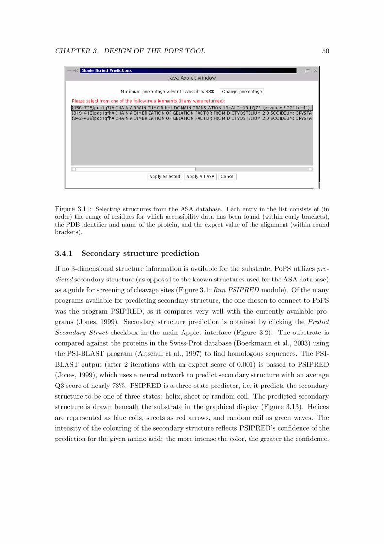
CHAPTER 3. DESIGN OF THE POPS TOOL 50
Figure 3.11: Selecting structures from the ASA database. Each entry in the list consists of (inorder) the range of residues for which accessibility data has been found (within curly brackets),the PDB identifier and name of the protein, and the expect value of the alignment (within roundbrackets).
3.4.1 Secondary structure prediction
If no 3-dimensional structure information is available for the substrate, PoPS utilizes pre-
dicted secondary structure (as opposed to the known structures used for the ASA database)
as a guide for screening of cleavage sites (Figure 3.1: Run PSIPRED module). Of the many
programs available for predicting secondary structure, the one chosen to connect to PoPS
was the program PSIPRED, as it compares very well with the currently available pro-
grams (Jones, 1999). Secondary structure prediction is obtained by clicking the Predict
Secondary Struct checkbox in the main Applet interface (Figure 3.2). The substrate is
compared against the proteins in the Swiss-Prot database (Boeckmann et al., 2003) using
the PSI-BLAST program (Altschul et al., 1997) to find homologous sequences. The PSI-
BLAST output (after 2 iterations with an expect score of 0.001) is passed to PSIPRED
(Jones, 1999), which uses a neural network to predict secondary structure with an average
Q3 score of nearly 78%. PSIPRED is a three-state predictor, i.e. it predicts the secondary
structure to be one of three states: helix, sheet or random coil. The predicted secondary
structure is drawn beneath the substrate in the graphical display (Figure 3.13). Helices
are represented as blue coils, sheets as red arrows, and random coil as green waves. The
intensity of the colouring of the secondary structure reflects PSIPRED’s confidence of the
prediction for the given amino acid: the more intense the color, the greater the confidence.

CHAPTER 3. DESIGN OF THE POPS TOOL 51
Figure 3.12: Results display with DSSP secondary structure and accessibility shown. Residuespredicted as inaccessible are shaded grey in the grahical display. Cleavages with associated inac-cessible residues are also shaded grey, in both the graphical and textual displays. The secondarystructure is drawn below the substrate using the DSSP single-letter code.
3.5 Prediction of PEST sequences
The existence of PEST sequences was originally proposed in 1986 as a target for rapid
degradation of cellular proteins (Rogers et al., 1986). PEST sequences are hydrophilic
stretches of at least 12 amino acids in length, distinguished by the presence of at least one
Pro (P) residue, one Asp (D) or Glu (E) residue, and one Ser (S) or Thr (T) residue (Rech-
steiner and Rogers, 1996). The entire region is flanked by positively charged residues,
i.e. Lys (K), Arg (R) or His (H) residues, but positively charged residues are not al-
lowed within the PEST region itself (Rechsteiner and Rogers, 1996). PEST regions are
Figure 3.13: Graphical display of the results panel showing predicted secondary structure ascomputed by the PSIPRED program, which predicts three states of secondary structure: helix(blue coils), sheet (red arrows), and random coil (green waves).

CHAPTER 3. DESIGN OF THE POPS TOOL 52
Figure 3.14: Graphical display of the results panel showing predicted PEST regions as computedby the PESTfind program. Potential PEST sequences are drawn with the ‘+’ symbol in green,poor potential PEST sequences are drawn with the ‘-’ symbol in aqua, and invalid PEST sequences(not shown) are drawn with a circle (‘o’) in grey.
widely distributed, comprising approximately 10% of the cellular proteins in the organisms
that have been analysed, and are typically located in proteins that are highly regulated
(Mitchell and Bell, 2003). PEST regions appear to target proteins for degradation by the
26S proteasome (Rechsteiner and Rogers, 1996), and sometimes calpain (Rechsteiner and
Rogers, 1996; Mitchell and Bell, 2003; Fukuda and Takashi, 2004; Tompa et al., 2004).
In addition, the regulatory and catalytic subunits of cAMP-dependent protein kinase of
Blastocladiella emersonii contain PEST sequences that target them for degradation by a
protease other than the proteasome (Borges and Gomes, 2000). Finally, the hydrophilic
nature of PEST sequences makes it likely that they form solvent-exposed loops or exten-
sions (Rechsteiner and Rogers, 1996). Sequences that are at the surface of the substrate
structure (rather than buried in the interior) are more likely to be accessible to the protease
for cleavage.
Thus, prediction of PEST sequences may prove useful in identifying potential cleavage
sites, either because the protease may specifically target PEST sequences or simply because
it identifies a region that is solvent accessible and therefore accessible to the protease.
PEST regions are calculated when the Find PEST regions checkbox is selected in the
main Applet interface (Figure 3.2), and PoPS uses the PESTfind program to predict
PEST regions in the substrate (Figure 3.14). The default PEST window size (minimum
distance between the flanking residues K, R or H) is set to 10 residues, which is the default
for the PESTfind program. The PEST predictions are drawn in the results display, below
the substrate sequence. Good or potential PEST sequences are drawn with the plus (‘+’)
symbol in green, poor potential PEST sequences are drawn with the minus (‘-’) symbol in
aqua, and invalid PEST sequences (not shown in the example) are drawn with the symbol
‘o’ in grey.
In summary, the accessibility, secondary structure and PEST information provided by
PoPS allows the user to screen predictions based not only on the score from the model,
but also on the basis of the structure of the cleavage site and surrounding regions. In the
previous figures, each prediction of structural information has been shown individually,

CHAPTER 3. DESIGN OF THE POPS TOOL 53
but it is, of course, possible to view all this information simultaneously in the graphical
display (Figure 3.5). As mentioned in Section 3.3, the graphical results display allows the
cleavage site to be viewed in the context of surrounding regions, to help the screening
process (Figure 3.5:A). In addition, a larger view of this graphical display can be opened
in a separate Java Applet window (Figure 3.5:B), which broadens this contextual view
even further.
3.6 Comparing different models of the same protease using
ROC curves
To allow users to measure the accuracy of specificity models, the PoPS system provides
a module for producing receiver operating characteristic (ROC) curves (Figure 3.1: ROC
curves module and Figure 3.16). ROC curves measure the ability of a model to correctly
assign high scores to true cleavages (true positives), and assign low scores to sites which
are not cleaved (true negatives) (Sorribas et al., 2002). The sensitivity of the model is
the proportion of true positives identified by the model, or the true positive rate. The
specificity of the model is 1 - the false positive rate, i.e. the proportion of true negatives
identified by the model. A ROC curve is a plot of the true positive rate against the
false positive rate, i.e. the sensitivity of the model against 1-specificity (Figure 3.16).
Given information regarding known cleaved and uncleaved sites (true positives and true
negatives), ROC curves can not only be used to measure how well an individual model is
able to identify the true cleavages from the uncleaved sites, but also to compare multiple
models for the same protease.
Like the main interface, the ROC curves module is provided as a Java Applet (Fig-
ure 3.16), which was partly implemented by Stewart Hore (BHP Billiton, Melbourne,
Australia). The use of an Applet was again chosen because it allows the easy implemen-
tation of a complex graphical interface for the program, enabling the user to create and
manipulate the ROC curves, and also produces a module that fits into the web-based
design of the PoPS system. Since the Applet is downloaded and executed on the user’s
machine, this also allows reasonably fast execution of the program.
The current implementation of the ROC curve calculation uses an empirical technique,
which fits a curve between the sample points without assuming an underlying distribution
of the data (i.e. the predicted cleavages) (Sorribas et al., 2002). A set of thresholds is
calculated from each unique pair of PoPS scores, and used to classify the scores as positive
or negative using the following predicate rule:
• If the score is greater than or equal to the threshold value, then it is positive;
• Otherwise, it is negative.

CHAPTER 3. DESIGN OF THE POPS TOOL 54
A
B
Figure 3.15: Graphical display of the results panel (A) and the larger graphical results window(B), with all structural predictions shown.

CHAPTER 3. DESIGN OF THE POPS TOOL 55
Figure 3.16: ROC curves Applet interface. The area under a ROC curve provides a useful measureof the model, where the optimal curve follows the left-hand, top border of the axes, with an areaof 1.0 (roc.1, shown in red). A ROC curve following a 45 degree line has an area of 0.5 (roc.2,shown in blue). Models with an area of 0.5 or less would have very little predictive value.

CHAPTER 3. DESIGN OF THE POPS TOOL 56
Because the true cleavage state (i.e. cleaved or not cleaved) for each score is known,
the true-positive (TP), true-negative (TN), false-positive (FP) and false-negative (FN)
values can be calculated. These are then used to calculate the false-positive rate, or 1-
specificity (X coordinate) and the true-positive rate, or sensitivity (Y coordinate) of a
point as follows:
False positive rate = 1 − Specificity = 1 −
[
TN
(TN + FP )
]
(3.1)
True positive rate = Sensitivity =TP
TP + FN(3.2)
The greater the sensitivity at high specificity values (i.e. high Y-axis values at low
X-axis values) the better the result (Figure 3.16). Thus, a ROC curve which follows the
left-hand, top border indicates a greater accuracy than one which lies along a 45 degree
line. Probably the most important information that can be obtained from the ROC curve
is the area under the curve. Once the plot has been generated, the area under the curve
is calculated using the trapezoid rule, implemented as:
A =
∫
f(x)dx =N−1∑
i=1
[
(Xi+1 + Xi)
2
]
(Yi+1 + Yi) (3.3)
where Xi and Yi denote the ith X and Y coordinate of each curve point. This value is a
measure of the accuracy of the PoPS predictions, and therefore of the model, for a given
experiment. The quantitative-qualitative relationship between area and accuracy follows
a fairly linear pattern, which can be interpreted as follows:
• 0.9-1: Excellent (1.0 indicating near perfect results);
• 0.8-0.9: Very good;
• 0.7-0.8: Good;
• 0.6-0.7: Average;
• 0.5-0.6: Poor (0.5 indicating meaningless results).
The ROC curve module allows the user to enter and edit ROC curve data through
the Create Plot Data and Edit Plot Data buttons, respectively (Figure 3.16). In addition,
users can load ROC curve data from a text file stored on their own computer. The user
can load multiple ROC curves at once, which are shown both as a list and in the legend at
the bottom of the Applet, and are graphed on the large canvas. The Applet provides the
facility to switch each individual ROC curve between being visible (located in the Graph
list) and not visible (Don’t Graph list). Lastly, the user can save the image of the ROC
curve to disk in portable network graphic (‘.png’) format.

CHAPTER 3. DESIGN OF THE POPS TOOL 57
3.7 Analysis of proteomic data and batch predictions
Models can not only be applied to single substrates, but also to the entire proteomic data
(i.e. all proteins) of any organism currently available in PoPS (Figure 3.1:Proteome/batch
predictions module), which includes:
1. Homo sapiens (human): 27,975 proteins;
2. Saccharomyces cerevisiae (baker’s yeast): 5,876 proteins;
3. Escherichia coli K12 : 4,242 proteins;
4. Drosophila melanogaster (fruit fly): 19,954 proteins;
5. Arabidopsis thaliana (thale cress): 29,157 proteins;
6. Rattus norvegicus (Norway rat): 22,849 proteins;
7. Mus musculus (house mouse): 26,549 proteins;
8. Danio rerio (zebrafish): 4,419 proteins;
9. Plasmodium falciparum (malaria): 5270 proteins;
10. Human herpesvirus 8 : 869 proteins (Swiss-Prot: 4, TrEMBL: 865);
11. Schistosoma mansoni (Blood fluke): 410 proteins (Swiss-Prot: 81, TrEMBL: 329).
The first nine of these proteome databases are obtained from NCBI’s Reference Se-
quence (RefSeq) database (http://www.ncbi.nlm.nih.gov/) (Pruitt et al., 2003), while the
last two come from the Swiss-Prot and TrEMBL databases (http://us.expasy.org/sprot/)
(Boeckmann et al., 2003). All of these databases are stored locally on the PoPS server in
a MySQL database. As in the case of the Models database, MySQL was chosen for the
proteome databases because of its attributes of speed, portability, flexible search mecha-
nism, and capability of managing the volume of data associated with such large databases.
Analysing an entire proteome takes too long to provide an interactive interface for the user.
Therefore, proteome searching is provided as a web-based HTML form, which takes as in-
put the user’s email, model and preferred organism. The results are returned to the user
by e-mail, with two different analyses of the output made available to the user. The first is
a set histograms which plot the frequency of the number of cleavages within the substrates
returned, and the frequency of maximum scores in the substrates. These histograms are
available with and without buried sites included in the analysis. The second analysis of
the output is two text files containing the hits from the proteome analysis: one containing
only the name and maximum score for each protein, the other also containing a reasoning
table showing the predicted scores. For each site, a summary of the solvent accessibility
and secondary structure data from DSSP is included for up to the top 5 structures avail-
able for the site (from the ASA database). The web input form allows the user to select a
number of parameters to screen the results. These parameters include selecting a cut-off
value for the scores returned, and choosing to receive only substrates containing less than
a given number of cleavages. The output can also be screened using options related to the

CHAPTER 3. DESIGN OF THE POPS TOOL 58
accessibility and secondary structure of the sites. For example, the user might want sites
with more than three buried residues to be removed from the output, or might want to
only view sites with more than three unstructured residues.
A second web-based HTML form is also available to do batch predictions of substrate
cleavage using a substrate file in fasta format (described previously in Section 3.4). Like
the proteome form, the batch prediction input includes the user’s email and the model
file, but instead of a proteome selection, the form takes as input a substrate sequence file
in fasta format. The batch prediction form allows the same screening options as for the
proteome analysis, and the output is in the same format as for the proteome predictions.
The proteomic and fasta file analyses are intended to be used with specificity models that
are already known to be reasonably accurate.
The option of screening batch predictions and whole proteomes has also been provided
by the PEPS (Lohmuller et al., 2003) and PrediSi (Hiller et al., 2004) programs, first
introduced in Chapter 2, Section 2.1. As mentioned before, the format of the PEPS and
PrediSi models are such that both these programs should produce the same results as
PoPS, except for a PoPS model that incorporates dependency rules. PEPS has been
applied to human and mouse protein databases from Swiss-Prot, while PrediSi allows
the user to submit protein sequence files in fasta format. Neither of the programs allow
structural screening of the results, and, again, both programs are limited to the inbuilt
models provided.
3.8 Conclusions
This chapter has described the development and implementation of the PoPS tool. The
web-based design allows PoPS to be widely accessible and does not require users to have
specialist computer knowledge to download or install the tool. The PoPS tool itself consists
of a series of modules that allow the investigation of substrate specificity, the accuracy of
models, possible cleavage of substrates, and the prediction of new substrates. The tool
also allows the user to investigate effects other than sequence specificity that may influence
cleavage. Currently, the tool implements methods to assess the accessibility and secondary
structure of cleavage sites, and the location of surrounding PEST regions. Overall, the
PoPS tool has been designed to maximise the number of operations that can be run locally
on the user’s computer (to maximise performance), and to allow users to save and load
data to and from their own computer. However, some critical operations are executed
on the server and users are encouraged to save their final models into the central PoPS
models database. Importantly, the modular design of the tool enables it to be modified and
maintained easily, and also allows the addition of further analysis tools. The end result
is a powerful, flexible tool that provides the key components for investigating protease
specificity, with a design that allows future work to be easily added.

CHAPTER 3. DESIGN OF THE POPS TOOL 59
The core component of the tool, the PoPS specificity model, has been developed to
represent the sequence specificity of the subsites, the relative importance of the subsites,
and the complex cooperative effects of specificity that can be seen in some proteases.
A model can be developed for any protease using any source of data available, from
experimental data to expert knowledge, and provides the user the flexibility to express
even subtle features of specificity. By restricting the range of values that can be used in the
PSSM, the model can be easily created and interpreted by human users. However, despite
the restricted range of values for the specificity profiles, the use of floating point values
in the PSSM, and the use of the weight vector in the score calculation, minimise loss of
information from the original data. To assist researchers in accessing knowledge of protease
specificity, the PoPS tool also provides a database of specificity models, which mirrors the
protease classification mechanisms of the well known MEROPS database (Rawlings and
Barrett, 1999). Using this existing classification system allows researchers to investigate
proteases using a familiar environment.
The PoPS specificity model predicts cleavage on the basis of primary sequence prefer-
ences. Therefore, potential cleavage sites can be predicted in regions of the substrate that
are structurally inaccessible to the protease, according to secondary or tertiary structure.
PoPS provides the facility to identify and screen out these regions by using either known
structure, if available, or predictive methods. In addition, the tool also allows the user
to identify possible PEST regions, to locate sites that might be more likely to be cleaved
(due to being more accessible, or being signalled for cleavage by the presence of the PEST
region itself).
Further modules are also provided for additional functionality. One of these is a pro-
gram to create ROC curves, to measure and compare the accuracy of specificity models.
The other two modules allow the user to screen batch files of substrates and entire pro-
teomes for possible targets. The batch/proteome predictions provide multiple output
formats, and allow the user to screen predictions by score threshold and structure.
As described previously, the programs PEPS and PrediSi are available for predicting
cysteine endopeptidase specificity and signal peptide cleavage, respectively, for individual
substrates, batch files and whole proteomes. The core matrix-based models of these two
systems will produce the same predictions as the combined PoPS PSSM and weight vector,
assuming the matrices are equivalent. However, neither PEPS nor PrediSi can express
cooperative effects, which are expressed in PoPS with the optional dependency rules.
Furthermore, neither program incorporates the structural screening provided by PoPS.
Certainly, the predictions from these programs could be passed to the same tools that are
used in the PoPS system, but a major advantage of PoPS is that all of this functionality is
provided within the same interface, and the system design allows easy addition of further
functionality in the future.

CHAPTER 3. DESIGN OF THE POPS TOOL 60
Thus, the PoPS system is a powerful, flexible collection of modules that provides a wide
range of functionality to complement protease research. The next chapter will illustrate
how this functionality can be applied to protease research, using three case studies as
examples.

Chapter 4
Evaluation
As discussed in Chapter 1 (Section 1.1), proteases are classified into seven different cat-
alytic classes (including the unknown catalytic type). This section illustrates the exper-
imental and informed processes supported by PoPS with case studies covering proteases
from three of the seven classes, specifically the cysteine, serine and metallo proteases.
The first case study investigates the specificity of proteases from the family of proteases
known as the caspases. The caspases are cysteine proteases that are involved in apoptosis
(cell death) and inflammation. This case study will focus on the specificity of caspase 1,
caspase 3 and caspase 8. Firstly, experimental data is used to create a PoPS specificity
model for the proteases. Then, these models are used to examine the cleavage sites in
known substrates of each caspase. The performance of the models is measured using
ROC curves, and then the models are used to predict potential new targets in the human
proteome. Finally, some preliminary data is presented of in vitro testing of three of the
predicted caspase 8 targets.
The second case study presents two serine proteases, thrombin and blood coagula-
tion factor Xa. These two proteases are important for the process of blood coagulation.
Experimental data is again used to create specificity models, which are then tested on
known cleavage sites/substrates, and ROC curves are used to measure the performance
of the models. Finally, for each protease, predicted targets from the human proteome are
assessed for the likelihood of being true substrates.
The third case study focuses on a metalloprotease called membrane-type matrix met-
alloprotease 1 (MT1-MMP). Like other matrix metalloproteases, this protease is known
for cleaving substrates that are found in the extracellular matrix. However, this protease
has also been observed to have an alternative specificity profile that does not match the
known matrix substrates. Instead, this thesis presents the hypothesis that this second
mode is selective for proteins of the centrosome. In this case study, expert knowledge
is used to create specificity models to investigate these two binding modes, one selective
for centrosomal proteins, and the other selective for the traditional extracellular matrix
61

CHAPTER 4. EVALUATION 62
proteins. The relevance of the models to centrosomal proteins is assessed, then the model
selective for centrosomal proteins is used to predict possible new centrosomal targets. The
case study concludes by presenting recent experimental work that has been conducted to
verify one of these targets, the protein pericentrin 2.
4.1 Case study 1: caspases 1, 3 and 8
The family of caspases are a structurally related group of cysteine proteases that share an
unusual and almost absolute preference for an Asp residue at the P1 position (Stennicke
and Salvesen, 1998; Earnshaw et al., 1999). Thus, the name ‘caspase’ derives from them
being cysteine proteases with a preference for aspartate, where the ase ending is the
formal nomenclature for enzymes. Caspases have very important physiological functions,
and cleave large numbers of substrates (Fischer et al., 2003). Some of these cleavages have
a specific and vital function, activating or inactivating their targets, while other cleavages
are almost incidental, occurring only as a result of a favourable caspase cleavage sequence
(Stennicke and Salvesen, 1998; Fischer et al., 2003).
The family of caspases are functionally classified into two groups. The first group
includes the caspases that promote apoptosis, a process in which a cell activates its own
destruction and death. The second group includes the caspases that mediate inflammation,
and particularly the generation of pro-inflammatory cytokines (Stennicke and Salvesen,
1998; Earnshaw et al., 1999; Thornberry et al., 1997, 2000; Creagh et al., 2003). Both
caspase 3 and caspase 8 belong to the first group of apoptotic caspases. Caspase 3 has
a specific role in the ‘downstream’ apoptotic events, which involve the destruction and
dismantling of the cell, while caspase 8 is involved in the ‘upstream’ signalling pathways
and the activation of the downstream caspases (Thornberry et al., 1997, 2000). Caspase 1,
on the other hand, belongs to the second group of caspases mediating inflammation and
cytokine maturation (Thornberry et al., 1997, 2000; Creagh et al., 2003). Since caspase 1
lacks a preference for the hydrophobic amino acids at P4 that are commonly observed in
the apoptotic substrates, it is not classified as an apoptotic caspase (Thornberry et al.,
1997), even though many immune reactions generated by caspase 1 ultimately result in
apoptosis (Creagh et al., 2003).
4.1.1 Developing specificity models for the caspases
To help determine caspase function and substrates, the specificities of caspases 1, 3 and
8 have been experimentally investigated. The S4 to S2 subsites have been profiled using
positional scanning synthetic combinatorial libraries (PS-SCL) (Thornberry et al., 1997,
2000), while the S4, S1 and S′
1 subsites have been investigated using fluorescence-quenched
substrates (Stennicke et al., 2000). For the S4 subsite, the overlapping data from both

CHAPTER 4. EVALUATION 63
studies yielded similar specificity profiles, indicating the two data sources could be success-
fully combined into one PoPS specificity model. Since the PS-SCL data is more complete,
this data was used in preference to the fluorescence-quenched data when available. The
raw data from this study was provided by Nancy Thornberry and Margarita Garcia-Calvo
(Merck & Co. Inc., Whitehouse Station, New Jersey, USA). The PSSM was created by
scaling the S4-S2 PS-SCL data and the S ′
1 fluorescence quenched data to the range 0.0
to +5.0, and setting unprofiled amino acids to 0.0 (see Tables 4.1, 4.2 and 4.3). In the
PS-SCL study, the Cys and Met residues were not profiled because they are highly sus-
ceptible to oxidation, and therefore are difficult to use in the synthesis of the peptides.
The values for the Met residue can be approximated with norleucine, which was profiled
in the PS-SCL study, therefore these data were used in each subsite profile for the Met
residue value, while the values for the Cys residue were all set to 0.0 (i.e. no contribution,
positive or negative, to the specificity). In those cases (in either study) where the rate of
cleavage was too low to be determined, the profile value was set to -5.0.
Subsites S4 S3 S2 S1 S1’Weights 1 1 1 1 1
Gly 0.077 1.997 0.044 # 5.000Ala 0.240 2.084 0.905 # 0.537Val 0.351 2.187 0.560 # 0.120Leu 1.250 1.563 0.274 # 0.037Ile 0.428 1.139 0.965 # 0.000Pro 0.171 0.028 0.770 # -5.000Phe 2.303 1.245 0.642 # 0.259Tyr 2.748 0.893 0.777 # 0.389Trp 5.000 0.417 0.683 # 0.000Ser 0.163 1.665 0.782 # 2.037Thr 0.163 2.155 1.957 # 0.352Cys 0.000 0.000 0.000 # 0.000Met 1.678 1.457 0.977 # 0.000Asn 0.111 0.587 0.359 # 0.204Gln 0.111 3.146 0.570 # -5.000Asp 0.334 1.833 0.208 5.000 -5.000Glu 0.428 5.000 0.485 # -5.000Lys 0.020 0.249 0.349 # 0.065Arg 0.021 0.281 0.301 # 0.046His 0.488 0.854 5.000 # 0.000
Table 4.1: The caspase 1 PoPS specificity model.
Since caspases 1 and 8 can only accept an Asp residue at the P1 position (Stennicke
et al., 2000), the value for Asp in the S1 profile was set to +5.0 and every other residue
in this profile was set to ‘#’. For caspase 3, however, it was found that a Glu residue was
tolerated at the P1 position, although cleavage was reduced to 20,000-fold less than with
an Asp residue at the same position (Stennicke et al., 2000). Therefore, the value for Glu

CHAPTER 4. EVALUATION 64
Subsites S4 S3 S2 S1 S1’Weights 1 1 1 1 1
Gly 0.023 0.392 0.055 # 4.825Ala 0.111 1.647 0.889 # 3.925Val 0.137 1.499 5.000 # 0.098Leu 0.060 0.682 1.156 # 0.083Ile 0.107 0.688 3.656 # 0.000Pro 0.026 0.025 1.889 # 0.019Phe 0.066 1.344 0.886 # 1.575Tyr 0.058 1.222 0.684 # 1.588Trp 0.025 0.618 0.318 # 0.000Ser 0.220 1.439 0.115 # 5.000Thr 0.280 1.665 1.776 # 1.150Cys 0.000 0.000 0.000 # 0.000Met 0.019 0.842 1.084 # 0.000Asn 0.185 0.705 0.202 # 0.588Gln 0.047 1.938 0.124 # 0.148Asp 5.000 1.187 0.016 5.000 0.105Glu 0.256 5.000 0.027 0.000 0.060Lys 0.044 0.136 0.051 # 0.198Arg -5.000 0.176 0.274 # 0.350His 0.107 0.797 1.052 # 0.000
Table 4.2: The caspase 3 PoPS specificity model.
was set to 0.0 in the S1 profile for the caspase 3 model, to indicate that it is tolerated
but does not appear to make any significant contribution to substrate recognition. In all
cases, the weights for every subsite were set to 1.0 and no dependency rules were added.
The maximum obtainable score for each model is 25.0, while the minimum score (other
than -Infinity) is 5.0 for the caspase 1 and 8 models, and 0.0 for the caspase 3 model.
The caspase 1, 3 and 8 models are available from the PoPS models database using the
identifiers C14.001>Boyd>1.2, C14.003>Boyd>1.2 and C14.009>Boyd>1.2, respectively.
4.1.2 Evaluation of the caspase specificity models
To evaluate the models, a list of substrates with known cleavage sites was obtained for
caspases 1 and 3 (Earnshaw et al., 1999) and caspase 8 (Klaus Schultze-Osthoff and Ute
Fischer, Institute of Molecular Medicine, University of Dusseldorf, Germany: personal
communication). The PoPS main interface was then used to apply the three models
to their respective known substrates. Tables 4.4, 4.5 and 4.6 show a summary of these
results for caspase 1, 3 and 8, respectively. Note that the number of known caspase 3
cleavage sites (41 sites) is significantly larger than for caspase 1 (7 sites) and caspase 8 (12
sites). This could possibly be a reflection of the fact that caspase 3 has a higher biological
concentration and catalytic efficiency than many of the caspases, including caspases 1 and
8 (Stennicke et al., 2000).

CHAPTER 4. EVALUATION 65
Subsites S4 S3 S2 S1 S1’Weights 1 1 1 1 1
Gly 0.503 0.040 0.107 # 5.000Ala 2.144 0.169 1.524 # 0.887Val 3.506 0.438 4.072 # 0.015Leu 5.000 0.109 0.457 # 0.009Ile 2.813 0.129 3.643 # 0.000Pro 2.262 0.021 1.125 # -5.000Phe 1.086 0.136 0.859 # 0.309Tyr 1.181 0.118 1.010 # 0.347Trp 0.678 0.065 1.427 # 0.000Ser 1.037 0.135 0.826 # 2.751Thr 1.359 0.351 5.000 # 0.093Cys 0.000 0.000 0.000 # 0.000Met 1.437 0.171 1.524 # 0.000Asn 1.325 0.060 0.575 # 0.334Gln 0.491 0.633 0.425 # 0.008Asp 3.391 0.974 0.389 5.000 0.006Glu 2.172 5.000 0.863 # -5.000Lys 0.021 0.007 0.406 # 0.012Arg 0.045 0.013 0.385 # 0.017His 0.658 0.125 1.385 # 0.000
Table 4.3: The caspase 8 PoPS specificity model.
In each table of results, the first column indicates the name of the substrate (Substrate).
The second column represents the known cleavage site(s) (Cleavage Site) using the single-
letter amino acid code of the 5 amino acids for the P4-P′
1 positions, with a period (‘.’)
marking the location of the cleavage. The third column (Max. Score) reports the maximum
score obtained for the entire substrate. The next column (Site Score/Rank) reports the
score for the known cleavage site followed by the rank of that score compared to every
other score for the substrate. For example, in Table 4.4, the sequence for Pro-IL1β has a
maximum score of 18.2. The score for the cleavage site FEAD.G (with cleavage occurring
between D and G) is 18.2 with a rank of 1, meaning that this is the site with the highest
score in the Pro-IL1β sequence. The YVHD.A site (cleavage between D and A) has a
score of 15.5, with a rank of 2, indicating this site has the second-to-highest score in the
Pro-IL1β sequence.
In addition to primary sequence, it is also interesting to look at the structural context
of the cleavage sites, to see if they are predicted as accessible to the enzyme. The fifth
column of each table provides analysis from the DSSP program (Kabsch and Sander,
1983), which calculates the accessibility of the substrate with the default minimum of 33%
solvent accessibility (Acc. (Min. 33%)), as described in Chapter 3. If four or five residues
across the cleavage site have less than 33% solvent accessibility, the cleavage is reported
as inaccessible (‘No’ in the results tables). If three residues are predicted as buried, the

CHAPTER 4. EVALUATION 66
Site Acc. 2 2
Cleavage Max. Score/ (Min. Struct. Struct. PossibleSubstrate Site Score Rank 33%) DSSP PSIPRED PEST
FEAD.G 18.2/1 - - SCCCC PoorPro-IL1β1
YVHD.A18.2
15.5/2 Yes ???? CCCCC YV PoorPro-IL182 LESD.Y 12.4 12.4/1 - - CCCCC InvalidBcl-XL
3 HLAD.S 12.8 10.0/2 Yes S CCCCC PoorALAD.S 9.8/7 - - HHHHH Poor
Calpastatin LSSD.F 12.3 9.0/16 - - HCCCC PoorALDD.L 7.1/37 - - HHHHH Good
Table 4.4: Results for the caspase 1 specificity model over known caspase 1 cleavage sites. 1Pro-Interleukin1β; 2Pro-Interleukin 18; 3Long version of Bcl-2-related gene product X.
site is reported as partially accessible (‘Part’). If only two or fewer residues are buried,
the cleavage site is reported as accessible (‘Yes’). Cleavage sites for which accessibility
information was not found (indicating a lack of available structures) are identified with
a dash (‘-’). It is worth noting three cases for which this classification is not absolutely
clear. In Table 4.4, the YVHD.A cleavage for Pro-IL1β is classified as accessible, but
accessibility data was only available for the A residue in this cleavage site. In Table 4.5,
Stat 1 is classified as accessible, although no information was available for the M residue
of this cleavage point, and PKC θ was classified as buried because the VD residues had a
solvent accessibility of less than 33%, and there was no accessibility information for any
of the other positions.
The sixth column (2 Struct. DSSP) provides the secondary structure information for
each cleavage site determined by DSSP. Each symbol in this column represents the sec-
ondary structure for the respective amino acid in the cleavage site (shown in the Cleavage
Site column). The one-letter abbreviation is the same as provided by DSSP (introduced
in Chapter 3, Section 3.4). An underscore symbol (‘ ’) is used to indicate that no spe-
cific secondary structure was found by DSSP, and a question mark (‘?’) indicates that
secondary structure information was not available for the respective amino acid.
The next column in the table (2 Struct. PSIPRED) reports the secondary structure
of the cleavage site predicted by PSIPRED, as described in Chapter 3 (Jones, 1999). Each
letter represents the predicted secondary structure for the respective amino acid in the
cleavage site, with the three states predicted by PSIPRED represented as ‘C’ for coil, ‘H’
for helix and ‘S’ for sheet. Note that, unlike the DSSP program, PSIPRED does not rely
on known structures, so there are no missing entries for this column.
Finally, the last column of the results tables contains information about whether the
cleavage occurs within a potential PEST region (Possible PEST). This classification is
obtained directly from the output of the PESTfind program, introduced in Chapter 3
(Rechsteiner and Rogers, 1996). The minimum PEST sequence length was set to 10

CHAPTER 4. EVALUATION 67
Site Acc. 2 2
Cleavage Max. Score/ (Min. Struct. Struct. PossibleSubstrate Site Score Rank 33%) DSSP PSIPRED PEST
β-II Fodrin DEVD.S 25.0 25.0/1 Yes HHHHH HHHHH NonePARP1 DEVD.G 24.8 24.8/1 - - CCCCC Invalid
RFC1402 DEVD.G 24.8 24.8/1 No ETGGG CCCCC Invalidα-II Fodrin DETD.S 21.8 21.8/1 - - CCCCC NoneMEKK-13 DTVD.G 21.5 21.5/1 - - HHHHH InvalidRas-GAP4 DTVD.G 21.5 21.5/1 No SEEG CCCCC PoorD4-GDI5 DELD.S 21.2 21.2/1 Yes CCCCC Invalid
Rb protein6 DEAD.G 20.7 20.7/1 - - CCCCC InvalidDNA-PKcs7 DEVD.N 20.6 20.6/1 - - CHHCC Invalid
PKC θ8 DEVD.K 20.2 20.2/1 No ??TT? HHHHH PoorLamin B1 VEVD.S 20.1 20.1/1 - - SSCCC NonePP2A9 DEQD.S 20.1 20.1/1 Part S HH CCCCH Poor
cPLA(2)10 DELD.A 20.1 20.1/1 Yes HHHHH PoorCytokeratin VEVD.A 19.1/1 - - SSSCC Poor
18 DALD.S19.1
17.8/2 - - CCCCC InvalidGelsolin DQTD.G 18.5 18.5/1 Yes T SSS CCCCC Poor
Topoisomerase I DDVD.Y 17.8 17.8/1 - - CCCCC NoneAtrophin-1 DSLD.G 17.4 17.4/1 - - CCCCC PoorU1-70kDa11 DGPD.G 17.1 17.1/1 - - CCCCC GoodPresenilin-2 DSYD.S 17.1 17.1/1 - - CCCCC GoodHuntingtin DSVD.L 16.5 16.5/1 - - CCSSC InvalidIκB-α12 DRHD.S 16.2 16.2/1 - - HHCCC None
p21/WAF113 DHVD.L 15.9 15.9/1 - - HHCCC PoorPAK214 SHVD.G 15.8 15.8/1 - - CCCCC S Poor
p27KIP115 DPSD.S 15.1 15.1/1 - - CCCCC PoorPro-IL1616 SSTD.S 13.4 13.4/1 - - CCCCC Good
DETD.S 21.8/1 - - CCCCC InvalidICAD17
DAVD.T21.8
17.8/3 - - HHHHC InvalidFAK18 DQTD.S 19.2 18.7/2 - - CCCCC Poor
SSLD.A 11.7/3 Yes T S CCCCC NoneBcl-XL
19
HLAD.S13.1
11.7/4 Yes S CCCCC PoorHDM2/MDM220 DVPD.C 15.1 13.4/3 - - CCCCC Poor
Stat 1 21 MELD.G 17.3 16.0/4 Yes ? CCCCC InvalidDCC22 LSVD.R 19.9 11.9/4 - - CCCCC Poor
PKC δ23 DMQD.N 14.5 11.6/4 Part HHHHH CCCCC InvalidPITSLRE24 YVPD.S 20.1 13.5/6 - - CCCCC GoodCaMK IV25 PAPD.A 16.5 12.5/6 Yes SSTT CCCCC Poor
PKN26 LGTD.S 20.0 12.2/7 - - CCCCC PoorPRK227 DITD.C 25.0 12.5/7 - - CCCCC PoorNuMA28 DSLD.L 17.2 12.7/10 - - CCCCC Poor
Calpastatin LSSD.F 19.2 8.2/35 - - HCCCC Poor
Table 4.5: Results for the caspase 3 specificity model over known caspase 3 cleavage sites.1Poly(ADP-ribose) polymerase; 2140kDa subunit of DNA replication factor C; 3MEK kinase-1 4Ras GTPase-activating protein; 5Rho GDP-dissociation inhibitor D4; 6Retinoblastoma geneproduct; 7Catalytic subunit of DNA-dependent protein kinase; 8Protein Kinase C θ; 9Proteinphosphatase 2A; 10Cytosolic phospholipase 2A; 1170kDa component of U1 small nuclear ribonu-cleoprotein; 12α isoform of Rel/NF-κB inhibitors; 1321kDa inhibitor of cyclin-dependent kinases;14p21-activated protein kinase; 1527kDa cyclin dependent kinase inhibitor; 16Pro-Interleukin 16;17Inhibitor of the caspase-activated deoxyribonuclease; 18Focal adhesion kinase; 19Long versionof Bcl-2-related gene product X; 20Murine double-minute chromosome mdm2 oncogene; 21Signaltransducer and activator of transcription factor; 22Deleted in colorectal cancer; 23Protein Ki-nase C δ; 24PITSLREp34-cdc2-related protein kinase; 25Ca/calmodulin-dependent protein kinaseIV; 26Protein kinase C-like 1; 27Protein kinase C-like 2; 28Nuclear-mitotic apparatus protein.

CHAPTER 4. EVALUATION 68
Site Acc. 2 2
Cleavage Max. Score/ (Min. Struct. Struct. PossibleSubstrate Site Score Rank 33%) DSSP PSIPRED PEST
FLIP1 LEVD.G 24.07 24.07/1 Yes CCCCC PoorBID2 LQTD.G 20.63 20.63/1 Yes S HHCCC Poor
CaMKLK (Rat)3 DEND.G 18.97 18.97/1 - - CCCCC GoodBAP314 AAVD.G 16.38 16.38/1 - - HHHCC None
IETD.S 20.56/1 Yes B CCCCC InvalidProcaspase 3
ESMD.S20.56
11.58/7 Yes HHCCC InvalidDSVD.A 13.48/2 - - CCSSC Invalid
Procaspase 7IQAD.S
15.3412.72/4 Yes S S SSCCC Good
PARP5 DEVD.G 22.58 22.46/2 - - CCCCC InvalidPAK26 SHVD.G 17.67 15.23/3 - - CCCCC S PoorRIP7 LQLD.C 19.12 11.09/9 - - CCCCC Poor
Plectin ILRD.K 17.17 8.32/91 - - HHHHH None
Table 4.6: Results for the caspase 8 specificity model over known caspase 8 cleavage sites. 1CASP8and FADD-like apoptosis regulator; 2BH3 interacting domain death agonist; 3Serine/threonine-protein kinase Doublecortin-like and CAM kinase-like 1; 4Likely ortholog of mouse B-cellreceptor-associated protein 31; 5Poly(ADP-ribose) polymerase; 6p21-activated protein kinase;7Serine/threonine protein kinase RIP.
amino acids, and the threshold PEST score for discriminating weak from potential PEST
motifs was set to +5.0, which are the default settings for the PESTfind program. In the
table, potential PEST sequences are reported as ‘Good’, ‘Poor’, ‘Invalid’ (do not meet the
requirements of a PEST region), or ‘None’ (there is no potential PEST region) (Rechsteiner
and Rogers, 1996). In some cases, only part of the cleavage site overlaps with a PEST
region, and these cases are noted in the tables accordingly (see for example the YVHD.A
cleavage for Pro-IL1β in Table 4.4).
It is clear from the tables that the caspase models are able to identify a large number
of the true cleavage sites using the primary sequence (amino acid) preferences alone. The
most notable exceptions to this are calpastatin (a caspase 1 and 3 substrate), and plectin
(a caspase 8 substrate). The cleavage of both these substrates proved difficult to predict
on the basis on primary sequence alone. Calpastatin is an inhibitor of calpain, another
prominent protease in apoptosis. By cleaving calpastatin, caspases 1 and 3 could help
promote apoptosis (Wang et al., 1998). However, this cleavage, like many putative caspase
substrates, has only been tested in vitro (“in the test tube”). Demonstration of in vitro
cleavage does not necessarily translate to in vivo cleavage (i.e. cleavage within the living
cell) and, therefore, it is necessary to determine that such cleavages are biologically relevant
(Stennicke and Salvesen, 1998; Stennicke et al., 2000). In the case of plectin, though, this
protein is a known caspase 8 substrate (Klaus Schultze-Osthoff and Ute Fischer: personal
communication). The PoPS model thus indicates that the primary amino acid sequence
of plectin is not the sole or main factor in determining its cleavage. Other factors, such

CHAPTER 4. EVALUATION 69
Figure 4.1: The surrounding regions of the p21/WAF1 DHVD.L caspase 3 cleavage site revealthat the helix predicted for the DH residues of the site only extends across three residues, with thecleavage site otherwise being located within an extended region of random coil.
as secondary-site interactions, may enable cleavage of unfavourable sites. Alternatively, it
may be intentional that the cleavage occurs slowly at intracellular concentrations of the
caspase (Stennicke et al., 2000).
Regarding structural information about the cleavage sites, the data shown in the tables
indicate that, for those sites where accessibility data is available, the cleavage sites are
also generally predicted as accessible. For the prediction of secondary structure, random
coil or sheet might be positive indicators for cleavage, but helices might be a negative
indicator. Again, most cleavages are predicted as having secondary structure that would
allow them to be cleaved easily. It is also interesting to note the number of potential
(‘Poor’ or ‘Good’) PEST sequences predicted for the cleavage sites. All but one of the
caspase 1 sites and more than half of the caspase 3 sites are located in a poor or good
PEST sequence, although predominantly these are poor PEST sequences. Possibly these
regions are sufficiently hydrophilic to be located on the exterior of the protein structure,
making the site more accessible to the protease.
It is important to note that while Tables 4.4, 4.5 and 4.6 provide comprehensive sum-
maries of the PoPS output, some information that is available when studying the predicted
cleavage of single substrates is lost. For example, Figure 4.1 shows the surrounding regions
of the p21/WAF1 DHVD.L caspase 3 cleavage site. The predicted secondary structure
across the active site includes helix as well as coil, which might be a negative indicator for
cleavage. However, when viewed in the context of the whole sequence, it becomes clear
that the predicted helix (which is weakly predicted) only extends across three residues, in
an extended region of predicted random coil. This structural conformation may present
the substrate to the protease in a better orientation for cleavage than the 5-residue sum-
mary of Table 4.5 suggested, thus explaining the cleavage site at the level of primary
sequence as well as structure. Therefore, while summary tables such as those presented
here are useful, a detailed study of each substrate is also needed for a complete view of
the predicted cleavage sites.

CHAPTER 4. EVALUATION 70
4.1.3 Comparing and measuring the caspase models with ROC curves
To measure the performance of the three caspase models, ROC curves (see Section 3.6)
were produced for each model using the substrates in Tables 4.4, 4.5 and 4.6. For each
protease, the known cleavage sites (shown in the respective tables) were used as the true
positives, and all other positions with an Asp residue at the P1 position were classified as
true negatives. In addition, for caspase 3 all sites with a Glu residue at the P1 position
were also classified as true negatives, since this amino acid has been shown to be tolerated
at this position (Stennicke et al., 2000). Only these (sub)-sequences in the substrate were
considered, because including positions without an Asp residue in P1 (and a Glu residue
for caspase 3) would bias the ROC curves in favour of the models. The curves, shown in
Figure 4.2, provide evidence that all three models are accurate for predicting cleavage of
their substrates: for caspase 1, the area under the curve is 0.85, for caspase 3 it is 0.98,
and for caspase 8 the area is 0.90.
For comparison, the caspase specificity models from the program PeptideCutter were
also used to examine the cleavage of the respective caspase substrates and generate ROC
curves (Figure 4.2). The same classification for the true positive/true negative sites was
used as for the ROC curves of the PoPS specificity models (described above). It is im-
mediately clear from these curves that the PoPS models show far more specificity and
sensitivity in predicting the caspase cleavage sites than the simple pattern-matching mod-
els of PeptideCutter.
Note that the program Cutter could not be compared to PoPS because it does not
provide models for the caspases. The program PEPS was also not compared to PoPS
because it uses the same matrix representation for the specificity model. Therefore, the two
programs should be able to produce the same results as long as the models are equivalent.
As mentioned in Chapter 3, ROC curves can also be used to compare the performance
of multiple models for the same protease in order to choose the best model. For example,
early in the development of the caspase 1 model, another 5 different models were produced
for this protease using different combinations of the measured experimental data mentioned
above, and general observations of behaviour, i.e. “expert knowledge” (Earnshaw et al.,
1999; Stennicke and Salvesen, 1998; Black et al., 1989; Sleath et al., 1990). The ROC
curves resulting from applying each model to the substrates shown in Table 4.4 are shown
in Figure 4.3. Generally, the models incorporating measured data (models A, B, E and F)
perform better than those using only expert knowledge (models C and D), although they
all seem to perform reasonably well. However, it was clear that model F (the caspase 1
model shown in the case study so far) was the best model. This model was constructed
using only experimental data, compared with the least successful model C, which was
constructed using only expert knowledge. It is interesting to note, however, that the ROC
curve suggests that even using only expert knowledge produces a model with some limited

CHAPTER 4. EVALUATION 71
Figure 4.2: ROC curves for the caspase 1, 3 and 8 specificity models from PoPS and PeptideCutter.
predictive value, although it is clearly not the best approach. Similar results were also
observed for caspase 3 (data not shown). From this it would seem that it is possible
to generalise the preferences for all three caspases using expert knowledge, but that the
experimental data is able to express subtleties that produce a better model overall.
4.1.4 Predicting new targets for the caspases
The ROC curves generated for the caspase 1, 3 and 8 models, and particularly for caspase 3,
suggest that their accuracy is reasonably high, and can therefore be used to search for new
targets. All three models were thus used to search the human proteome, which currently
consists of 27,975 proteins. In an initial screening, the proteome was searched with the
relatively low threshold of 10.0 (compared to the maximum scores of the models), with no
limits set on the structure or the number of scores in a substrate. The goal of this first

CHAPTER 4. EVALUATION 72
Figure 4.3: ROC curves for the different models constructed for caspase 1. A: experimentaldata (Thornberry et al., 2000). B: expert knowledge (Black et al., 1989; Sleath et al., 1990) andexperimental data (Thornberry et al., 2000). C: expert knowledge (Stennicke and Salvesen, 1998).D: expert knowledge (Earnshaw et al., 1999). E: expert knowledge (Black et al., 1989; Sleathet al., 1990; Stennicke and Salvesen, 1998) and experimental data (Thornberry et al., 2000). F:experimental data (Stennicke et al., 2000; Thornberry et al., 2000).

CHAPTER 4. EVALUATION 73
Figure 4.4: Histogram of the human proteome analysis for caspase 1, showing the distributionof the maximum scores for the proteins returned, with the threshold score set to 10.0 and nostructural/score limits selected.
run was to obtain the distribution of the maximum scores across the proteome, and use
it to select a new threshold that would produce a reasonably small set of predictions for
analysis in the experiment presented here. The initial score of 10.0 was selected because
all enzymes have a requirement for an Asp residue at P1, and caspase 1 has a strong
preference for a Trp residue at P4, while caspase 3 and 8 have a strong preference for
an Asp residue at P4. Therefore, for all three caspases, if these conditions are satisfied,
the score must be at least 10.0 (although a score of >10.0 does not guarantee that the
conditions have been met). The histograms of the maximum scores returned (with buried
results included) are shown in Figures 4.4, 4.5 and 4.6.
From the histograms, the new threshold for the caspase 1 proteome analysis was se-
lected as 21.0, and for caspases 3 and 8 as 24.0, and the proteome analysis was repeated
for each. Tables 4.7, 4.8 and 4.9 show the list of hits from the caspase 1, 3 and 8 analysis
(respectively) with the new thresholds. The proteome search using the model for caspase 1
yielded a total of 34 proteins, caspase 3 a total of 33 proteins, and caspase 8 a total of 26
proteins. Each table contains the NCBI accession number and name of each protein, to-
gether with the score for the predicted cleavage site. For each result set, multiple isoforms
of proteins were grouped together to give a total of 22 unique proteins for caspase 1, and
24 unique proteins for both caspase 3 and caspase 8.

CHAPTER 4. EVALUATION 74
Figure 4.5: Histogram of the human proteome analysis for caspase 3, showing the distributionof the maximum scores for the proteins returned, with the threshold score set to 10.0 and nostructural/score limits selected.
Due to their restricted specificity, the caspases exhibit limited proteolysis of their sub-
strates, cleaving the substrate usually just once, in interdomain regions (Stennicke and
Salvesen, 1998). As described earlier, caspase 1 mediates inflammation and cytokine mat-
uration, and promotes events that can ultimately lead to apoptosis (Thornberry et al.,
1997; Creagh et al., 2003). Caspase 1 is expressed in a variety of cells of the immune
system and a number of tissues, and has been detected in proenzyme form in the cyto-
plasm, and in active form at the plasma membrane (Thornberry, 2004). As mentioned
previously, caspase 3 and 8 mediate apoptosis. Caspase 3 mRNA has been observed in
cell lines of the immune system, and cell lines of brain and embryonic origin (Nicholson
and Thornberry, 2004). Caspase 3 acts as an ‘executioner’ or ‘downstream’ protease in
apoptosis, and appears to inactivate proteins involved in cellular repair and homeostasis
(Thornberry et al., 1997; Creagh et al., 2003; Thornberry, 2004). Caspase 8 is an ‘initia-
tor’ or ‘upstream’ protease in apoptosis, affecting the signalling pathways and initiating
apoptosis in embryonic development, immune system maturation and in response to viral
infection (Thornberry et al., 1997; Creagh et al., 2003; Salvesen and Boatright, 2004).
The likelihood of each predicted target being a substrate was assessed by finding
the functional role of each protein using the NCBI database, which is publicly avail-
able online from http://www.ncbi.nlm.nih.gov/ (Pruitt et al., 2003) and the Swiss-Prot

CHAPTER 4. EVALUATION 75
Figure 4.6: Histogram of the human proteome analysis for caspase 8, showing the distributionof the maximum scores for the proteins returned, with the threshold score set to 10.0 and nostructural/score limits selected.
database, which is publicly available at http://us.expasy.org/sprot/ (Boeckmann et al.,
2003). Unless a specific reference is made, the details in the remainder of this sec-
tion are derived from these resources. If the functional role would make the protein
a logical target for the protease, the predicted site was further assessed for accessibil-
ity and structure using PoPS in the method described earlier, and the Pfam database
(http://www.sanger.ac.uk/Software/Pfam/) (Birney et al., 2002) was used to search for
the location of the cleavage with respect to protein domains. While there are too many
proteins to analyse in detail, some particularly interesting ones are discussed below. The
notations used to describe features of the cleavage site (consensus site, secondary structure,
accessibility and potential PEST regions) are those defined in Section 4.1.2.
For caspase 1 (Table 4.7), the first interesting prediction is Paxillin, a cytoskeletal pro-
tein involved in the actin-membrane attachment at sites of cell adhesion to the extracellular
matrix. Paxillin appears to modulate T cell migration, cell signalling and movement. In
particular, it has been implicated in signalling interactions between tumor cells and the
extracellular matrix. The predicted cleavage site, FEHD.G, occurs within the N-terminal
of the third LIM domain in a sequence of four, where LIM domains appear to act as an
interface for protein-protein interactions. Using PoPS, the site is predicted as accessible

CHAPTER 4. EVALUATION 76
NCBI PoPSAccession Substrate Description Score
NP 940846.1 GPAD9366 25.0NP 002850.1 Paxillin 22.3NP 055559.1 TBC1 domain family, member 5 22.3NP 002717.3 Prolyl endopeptidase 22.2XP 291485.3 Similar to Myosin-binding protein H 22.2NP 937791.1 Carboxypeptidase X (M14 family), member 2 22.2NP 000383.1 ATP-binding cassette, sub-family C, member 2 22.0NP 065816.1 Retinoblastoma-associated factor 600 22.0NP 067610.1NP 055059.1
Procollagen N-endopeptidase 21.7
NP 542453.2NP 631894.1
Metalloprotease-disintegrin protease 21.7
NP 001521.1NP 851397.1
Hypoxia-inducible factor 1, alpha subunit 21.7
NP 055058.1 Zinc metalloendopeptidase 21.7NP 006742.2 Sperm specific antigen 2 21.7NP 777572.1 Hypothetical protein FLJ31204 21.7NP 003742.2NP 874371.1
Eukaryotic translation initiation factor 3, subunit 9 η 21.7
NP 064630.1 Tubby like protein 4 21.7NP 597676.1NP 597681.1NP 596869.1 Connectin 21.6NP 596870.1NP 033310.2NP 620594.1NP 620595.1NP 620596.1
Von Willebrand factor-cleaving protease 21.3
NP 620597.1NP 061336.1NP 740754.1
McKusick-Kaufman syndrome protein 21.3
NP 001546.2 Immunoglobulin superfamily, member 1 21.3NP 849144.2 Immunoglobulin superfamily, member 10 21.3NP 149018.1 Leishmanolysin-like (metallopeptidase M8 family) 21.1
Table 4.7: The top scoring targets for caspase 1 from the human proteome analysis.
to the protease, it occurs across a hydrogen bonded turn connecting two extended strands
(EEETT), and the residues FE are predicted as being part of a poor PEST sequence.
Another predicted target, Prolyl endopeptidase, is found in the cytoplasm of human
lymphocytes and T cells (Vanhoof et al., 1994; Shirasawa et al., 1994). The predicted
cleavage, WTHD.G, is located within the peptidase S9 N domain, which protects the
catalytic triad of the peptidase, excluding larger cytosolic peptides and proteins from
proteolysis. The cleavage site is only partially accessible, with secondary structure of
a sheet extending into a hydrogen bonded turn and bend (E-TTS), and a poor PEST
sequence predicted immediately C-terminal of the cleavage site.

CHAPTER 4. EVALUATION 77
The protein Hypoxia-inducible factor 1 (HIF-1α) is found in the cytoplasm in nor-
moxia (normal oxygen conditions), but undergoes translocation to the nucleus in response
to hypoxia (low oxygen conditions). It is over expressed in the majority of common human
cancers and their metastases, due to intratumoral hypoxia, as well as mutations of genes
encoding oncoproteins and tumor supressors. The predicted cleavage, MEHD.G, has un-
known accessibility but is predicted to consist of helix and coil (HHHCC) by PSIPRED,
and has no associated PEST region. Interestingly, the predicted cleavage is located be-
tween residues 725-726 in the protein sequence. Immediately N-terminal to this site, at
residues 718-721, is a potential nuclear localisation signal. Mutation of this site (K719T),
or removal of the residues 653-826 prevents nuclear localisation of this protein (Sutter and
Semenza, 2000). If caspase 1 could cleave this site, it could prevent the localisation of
HIF-1α to the nucleus, and therefore prevent cellular adaptation to hypoxic conditions.
Leishmanolysin-like has the predicted cleavage site WIHD.G. This protein is localised
to the cell membrane, and has an inferred cell adhesion function. In particular, it has been
linked to cell defense mechanisms. The predicted site occurs towards the C-terminal of
the Peptidase M8 domain. There is no accessibility information, but the site is predicted
to have a sheet/coil secondary structure (SSCCC), and the WI residues are located in an
invalid PEST region, while the HDG residues are located in a poor PEST sequence.
Another interesting prediction is the ATP-binding cassette, an integral membrane pro-
tein found on the apical membrane of polarised cells in the liver, kidney and intestine. This
protein appears to confer resistance to anti-cancer drugs in mammalian cells. The cleav-
age site, WEHD.S, is predicted to be at least partly accessible to the protease ( EETT),
with the WE residues located within an invalid PEST region. C-terminal to the predicted
cleavage site is a poor PEST sequence. The cleavage site is located in a region predicted
to be cytoplasmic, between an ABC membrane domain and an ABC tran domain.
Caspase-mediated cleavage of Retinoblastoma protein by caspase 3 (see Table 4.5) has
been demonstrated to be essential for induction of apoptosis (Dou and An, 1998). It is
therefore interesting that Retinoblastoma-associated factor 600 is a predicted target of
caspase 1. The function and localisation of this protein is unknown, although it has a
predicted activity in the ubiquitin cycle. The structure of the cleavage site, WETD.G, is
unknown, but the predicted secondary structure (PSIPRED) is in a unstructured region
(CCCCC), and the site is located within a poor PEST region.
Finally, the set of predicted caspase 1 targets includes Immunoglobulin superfamily
members 1 and 10, and the protein Similar to myosin-binding protein H. While the function
of these three proteins is unknown, they all contain immunoglobulin domains and belong
to the immunoglobulin super-family. Proteins of this family play a role in cell recognition
and regulation of cell behaviour, which would make them all interesting caspase 1 targets.
It is interesting to note that the predicted targets for caspase 3 (shown in Table 4.8)
include substrates with known cleavage sites. These are Spectrin (βII-Fodrin), Protein

CHAPTER 4. EVALUATION 78
NCBI PoPSAccession Substrate Description Score
NP 055995.3NP 878914.1NP 878916.1 Nesprin 2 25.0NP 878917.1NP 878918.1NP 003119.1NP 842565.1
Spectrin, beta, non-erythrocytic 1 25.0
NP 071496.1NP 114381.1
Eukaryotic translation initiation factor 4H 25.0
NP 055761.2NP 955468.1
Spastin 25.0
XP 376587.1XP 374414.1
Similar to mKIAA0038 protein 25.0
NP 006247.1 Protein kinase C-like 2 25.0NP 689988.1 Hypothetical protein MGC33607 25.0NP 056161.2 Zinc finger, FYVE domain containing 26 25.0NP 060939.3 Uncharacterized hypothalamus protein HT008 25.0NP 005988.1 Transcription factor-like 1 25.0NP 775962.1 Chromosome 9 open reading frame 75 25.0NP 037377.1 Vacuolar protein sorting factor 4A 25.0NP 038476.2NP 872589.1
ATP-dependent chromatin remodeling protein 24.8
NP 001609.1 poly (ADP-ribose) polymerase family, member 1 24.8NP 002904.3 Replication factor C large subunit 24.8NP 003861.1 RasGAP-like with IQ motifs 24.8NP 064506.2 UDP-glucose:glycoprotein glucosyltransferase 2 24.8NP 775878.1 Chromosome 14 open reading frame 24 24.8NP 055855.1 1-phosphatidylinositol-4-phosphate 5-kinase 24.8NP 055876.1 Gene amplified in squamous cell carcinoma 1 24.8NP 005163.1 Atonal homolog 1 24.8NP 067025.1 P53-inducible protein 24.8NP 060717.1 Transmembrane protein 30A 24.8NP 006315.1 Craniofacial development protein 1 24.8
Table 4.8: The top scoring targets for caspase 3 from the human proteome analysis.
kinase C-like 2 (PRK2), Replication factor C large subunit (RFC140) and Poly(ADP-
ribosyl) polymerase (PARP), which were described in Section 4.1.2 (see Table 4.5). In
addition, there are a number of other predicted substrates with functions that would
make them likely targets of caspase 3.
Eukaryotic translation initiation factor 4H is a cytoplasmic protein that binds mRNA
and stimulates protein translation. Both isoforms have been found in fibroblasts, and the
spleen, testis and bone marrow, and the short isoform is also found in the liver and skeletal
muscle. The cleavage site, DEVD.S, is located toward the C-terminal end of the RRM 1
domain, and is predicted to be partially accessible, although it is located in a region that is

CHAPTER 4. EVALUATION 79
predicted to be inaccessible. The secondary structure indicates that the site is composed
of a bend/helix combination (SSHHH), located in an invalid PEST region.
Another predicted caspase 3 target is Spastin, a nuclear and perinuclear cytoplasmic
protein that is ubiquitously expressed. It is believed to be an ATPase that is involved in the
assembly or function of nuclear protein complexes, and possibly microtubule dynamics.
The cleavage site, DEVD.S, is predicted to have low solvent accessibility, between 25-
32% solvent accessible across the cleavage site, with the exception of the E residue which
is predicted as being only 3% solvent accessible. However, the site is predicted to be
unstructured, and the sequence is located within a poor PEST sequence.
The protein RasGAP-like with IQ motifs is a widely expressed structural protein, and
interacts with signalling and cell adhesion molecules and components of the cytoskeleton to
regulate cell morphology. The cleavage sequence, DEVD.G, occurs within the N-terminal
of the protein, and has no accessibility information, but is predicted to be composed of
helix/coil (HHCCC) by PSIPRED, and is located within an invalid PEST sequence.
Nesprin 2 is a nuclear transmembrane protein, with the largest part located within the
cytoplasm, and the C-terminal located in the nuclear envelope. This protein is involved in
maintaining nuclear organisation and structural integrity, possibly by tethering the nucleus
to the cytoplasm. The cleavage site, DEVD.S, is located in the cytoplasmic domain, close
to the transmembrane region. Although there is no accessibility information, the site
itself is predicted by PSIPRED to consist of random coil, and is located in a poor PEST
sequence.
Finally, there is a very interesting group of predicted caspase 3 targets that includes
Similar to mKIAA0038 protein, Transcription factor-like 1 and ATP-dependent chromatin
remodeling protein, all of which are proteins that are involved in DNA structure and
regulation, and would therefore make logical caspase 3 targets. A point to note is that
these three proteins are all nuclear proteins, whereas caspase 3, at least in its inactive
form, is located in the cytoplasm. This would normally suggest that these proteins are
unlikely to be caspase 3 substrates. However, it is also the case that well-known caspase 3
substrates, such as PARP and Rb protein (see Table 4.5), are also nuclear proteins. Since
apoptosis involves the regulated dismantling of cells and organelles, it would seem that
the dismantling of the nucleus allows caspase 3 to move into the nucleus and/or the target
substrates to move outwards. Therefore, it is likely that caspase 3 would at least be able
to access these substrates, if not actually cleave them.
The set of caspase 8 predictions also contains a number of interesting trends (Table 4.9).
As well as the known substrate FLIP (which was described in Section 4.1.2, and listed in
Table 4.6), another very interesting prediction is the Fanconi anemia (FANCC) protein.
The predicted cleavage site, LETD.G, is located in an invalid PEST region, and while
there are no known structures for this protein, the site is predicted by PSIPRED to be
unstructured (HCCCC). The function of this protein is still unknown, however, it has

CHAPTER 4. EVALUATION 80
NCBI PoPSAccession Substrate Description Score
NP 000928.1 DNA-directed RNA polymerase II, largest subunit 25.0NP 000127.1 Fanconi anemia, complementation group C 25.0NP 057680.2NP 056216.1
histone deacetylase 7A 25.0
NP 006175.2 Nucleobindin 1 25.0NP 079194.2 Chromosome 20 open reading frame 172 25.0NP 003628.2 Integrin, alpha 10 precursor 25.0NP 036587.1 ADP-ribosylation factor guanine nucleotide-exchange factor 6 25.0NP 055123.1 Phosphoinositide-3-kinase, regulatory subunit 25.0NP 919261.1 Hypothetical protein FLJ39441 25.0NP 620129.2 Chromosome 19 open reading frame 22 25.0NP 115873.1 LGP1 homolog 25.0NP 079033.3 Euchromatic histone methyltransferase 1 25.0NP 002153.1 Intercellular adhesion molecule 3 precursor 24.1NP 000811.1 Growth arrest-specific 6 24.1NP 055300.1 Prostaglandin-D synthase 24.1NP 150594.2NP 006449.2
Tripartite motif protein TRIM3 24.1
NP 001031.2 Sex hormone-binding globulin 24.1NP 004242.1 RAB9A, member RAS oncogene family 24.1NP 004111.2 Guanylate binding protein 2, interferon-inducible 24.1NP 060225.4 FLJ20303 protein 24.1NP 057454.1 RAB9-like protein 24.1XP 209097.2 Similar to FLJ10101 protein 24.1NP 110394.2 AT-hook transcription factor AKNA 24.1NP 003870.3 CASP8 and FADD-like apoptosis regulator 24.1
Table 4.9: The top scoring targets for caspase 8 from the human proteome analysis.
been shown to be regulated by a caspase during apoptosis (Brodeur et al., 2004). Two
cleavage sites have been identified, one of which is the predicted LETD.G site, the other
being KEMD.S. Not only does caspase 8 have a clear preference for this first cleavage
site, FANCC appears to suppress apoptosis upstream of caspase 3 activation, suggesting
caspase 8 is responsible for FANCC inactivation (Brodeur et al., 2004).
Two substrates, Tripartite motif protein TRIM3 (TRIM3) and RAB9A, member RAS
oncogene family (Rab9), are important for cellular trafficking. TRIM3, also known as
BERP, localises to cytoplasmic filaments, and is similar to a rat protein which is a specific
partner for the tail domain of myosin V. This protein is involved in the targeted transport of
organelles and, by homology, it appears that human TRIM3 may play a role in myosin V-
mediated cargo transport. The predicted cleavage sequence is LEVD.G. There are no
structures for this protein, but the predicted secondary structure is SCCCS, and the site
occurs within an invalid PEST region. Rab9 belongs to the Rab family of small GTPases.
This protein appears to be involved in the transport of proteins between the endosomes
and the trans Golgi network. The predicted cleavage site also occurs at the sequence

CHAPTER 4. EVALUATION 81
LEVD.G. The secondary structure for this site is E- -SS, and is predicted as accessible
to the protease. An invalid PEST region occurs at the C-terminal of the cleavage site
(beginning immediately C-terminal to the P ′
1 G residue).
The proteome predictions for caspase 8 also returned a number of signalling molecules.
Integrin alpha 10 precursor is a membrane protein that participates in cell adhesion as well
as cell signalling. A second signalling molecule is Phosphoinositide-3-kinase (PI3K), which
has a role in recruiting and activating PI3Kγ. Both of these proteins have a predicted
cleavage sequence, LETD.G, with unknown structure. The integrin site has a predicted
secondary structure of SSSCC, and is located in a poor PEST region, while the PI3K site
has a predicted secondary structure of HCCCC, and is located within a good PEST region.
Two other predicted signalling proteins are Intercellular adhesion molecule 3, and Growth
arrest-specific 6, both with a predicted cleavage site of LEVD.G. Intercellular adhesion
molecule 3 has no known structure, but has a predicted structure of SSSCC, and is located
in an invalid PEST region. The Growth arrest-specific 6 site is partially accessible, with
secondary structure EEETT, and is also located in an invalid PEST region.
In addition to signalling proteins, the proteome analysis returned a number of pro-
teins that regulate DNA structure and access, including DNA-directed RNA polymerase
II, Histone deacetylase 7A (HDAC7), nucleobindin 1 and AT-hook transcription factor
AKNA, all of which contained a predicted cleavage motif of LETD.G. The largest subunit
of DNA-directed RNA polymerase II forms part of the DNA binding groove on which
DNA is transcribed into RNA. Only two of the residues are predicted as accessible to the
protease, but one of these is the essential Asp (D) residue at P1, the other being the Glu
(E) residue at P3. The secondary structure is EEESS, and the site is located within an
invalid PEST region. In response to DNA damage, DNA-directed RNA polymerase II is
cleaved by a caspase, and in vitro cleavage of this protein by caspase 8 produces the same
sized fragments (Lu et al., 2002). Site-directed mutagenesis identified the cleavage site as
the LETD.G sequence (Lu et al., 2002), as predicted by PoPS.
The HDAC7 site, for both isoforms, is located within a poor PEST region, and has no
known structure, but has a predicted secondary structure of HHHCC. The nucleobindin 1
site is also located within an invalid PEST region, and again has no known structure,
but has a predicted secondary structure of HHCCH. Finally, AKNA is also involved in the
regulation of DNA structure, modifying the architecture of the DNA to allow transcription
factors access to promoters (Siddiqa et al., 2001). As mentioned earlier, caspase 8 plays
a role in the development of immune cells (Salvesen and Boatright, 2004), and AKNA
plays an important role during B cell differentiation (Siddiqa et al., 2001). The predicted
site, with motif LEVD.G, has unknown structure, but is predicted to have the secondary
structure SSSCC and is located in a good PEST region.
Whilst these predictions need to be tested for their biological relevance, it is interesting
to note that in such a large database of potential hits, some very interesting substrates

CHAPTER 4. EVALUATION 82
Caspase 8 (nM)
200
11697
66
45
31
21
14
kDa
Bid/Rab9
Rab9Bid
Caspase 8
small subunitCaspase 8
large subunit
100030010030100100030010030100
*
Figure 4.7: Bid and Rab9 cleavage by Caspase 8. While Bid is cleaved at higher concentrationsof caspase 8, Rab9 remains insensitive to caspase 8 even up to 1000nM of caspase 8. * indicatesthe band for the cleavage product of Rab9.
were returned, in particular proteins that would be logical targets for each specific cas-
pase, based on the biological function of both the substrate and the respective caspase.
The proteins discussed above clearly contain a sequence that would be favourable to the
respective caspase, although whether the secondary and tertiary structure at the predicted
site is conducive to cleavage remains to be tested. However, these results, in combination
with the results of Section 4.1.2, suggest that the primary sequence of proteins may play
an important role in the specificity of at least caspases 1, 3 and 8. Furthermore, the
results also suggest that PoPS is a powerful tool that allows protease biologists to screen
and search for potential targets.
4.1.5 Verifying predicted caspase 8 substrates
This section includes the unpublished experimental data of Fiona Scott (The Burnham
Institute, La Jolla, San Diego, U.S.A.). From the top 24 predicted caspase 8 targets shown
in Table 4.9 (Section 4.1.4), three of the likely targets were selected to be tested for in
vitro cleavage by caspase 8, specifically Rab9, TRIM3 and HDAC7.
First, Rab9 was tested for cleavage by caspase 8, using the known substrate Bid (see
Table 4.5) as a positive control. 6×His-tagged Rab9 and Bid were expressed in and purified
from BL21(DE3) E. coli. 1µM of Bid or Rab9 was incubated with 0, 10, 30, 100, 300 and
1000 nM active site titrated recombinant caspase-8 for 30 minutes at 37 degrees Celcius.
The samples were analysed by SDS-PAGE and Coomassie stained (see Figure 4.7). While

CHAPTER 4. EVALUATION 83
Figure 4.8: The structure of the predicted Rab9 caspase 8 cleavage site (Asp52Gly) occurs on atight bend, in a conformation that is unlikely to be able to fit into the catalytic groove of caspase 8.The image is generated using PyMol and the PDB structure 1WMS.
Bid is clearly processed by caspase 8, Rab9 remains insensitive to cleavage even at 1000 nM
caspase 8.
The top 5 structures for the Rab9 cleavage site suggest that the residues are mostly
accessible to the protease (BSBSS for all 5 structures). However, each of the structures
suggest that the cleavage site is located at a point where the secondary structure changes
from a beta strand into a non-hydrogen bonded turn, or a hydrogen-bonded turn (E- -SS
for one structure, EEETT for two structures, and EESSS for two further structures). A
closer look at the structure of the predicted cleavage site (Asp52Gly) reveals that these
two residues are certainly solvent accessible, but are located on a tight bend between two
beta strands (see Figure 4.8). As described in previous sections, caspase 8 requires contact
with the four residues N-terminal to the cleavage site (i.e. P4-P1) as well as the P ′
1 residue,
and the geometry of the turn may not allow this level contact, explaining why this site is
not cleaved.
The second experiment tested the in vitro cleavage of HDAC7 and TRIM3/BERP.
FLAG-tagged HDAC7 or TRIM3 cDNA were transfected into HEK293 cells. 48 hours
post-transfection, FLAG-tagged proteins were immunoprecipitated with monoclonal anti-
FLAG antibody. The immunocomplexes were incubated with 200 nM active site titrated
recombinant caspase 8 for 30 minutes at 37 degrees Celcius. Samples were analysed by
SDS-PAGE and immunoblotted with monoclonal anti-FLAG antibody.
From these results, TRIM3 clearly remains insensitive to caspase 8. The predicted
TRIM3 cleavage site is located between different protein-binding domains, so that cleavage

CHAPTER 4. EVALUATION 84
+−+−+− Caspase 8 (+/−)
HDAC7TRIM3/BERPCleaved HDAC7
Non−specificprotein
kDa209
12480
49
35
29
21
14
TRIM3/BERP HDAC7Vector
Figure 4.9: BERP/TRIM3 and HDAC7 cleavage by caspase 8. No cleavage of TRIM3/BERPwas observed, but HDAC7 was processed by caspase 8.
might cause disregulation of activity (F. Scott, personal communication). Why this site
was not cleaved is difficult to assess, due to the lack of available structures. The predicted
secondary structure is SCCCS and so, like Rab9, may be located on an unfavourable tight
turn. Alternatively (or in addition), the site may not be accessible to the protease due to
the tertiary structure of the substrate (i.e. may be buried internally).
However, the results clearly showed that HDAC7 was cleaved by caspase 8. To inves-
tigate the concentrations at which cleavage occurred, FLAG-tagged HDAC7 cDNA was
transfected into HEK293 cells. 48 hours post-transfection, FLAG-HDAC7 was immuno-
precipitated with monoclonal anti-FLAG antibody. Immunocomplexes were incubated
with 0, 4, 20, 100 and 500 nM active site titrated recombinant caspase-8 for 30 minutes
at 37 degrees Celcius. Samples were analysed by SDS-PAGE and immunoblotted with
monoclonal anti-FLAG antibody, and Figure 4.10 clearly shows that HDAC7 is cleaved
by caspase 8 at even relatively low concentrations.
Finally, cleavage of HDAC7 was tested against a series of apoptotic caspases: cas-
pases 2, 3, 6, 7, 8, 9 and 10. FLAG-tagged HDAC7 cDNA was transfected into HEK293
cells. 48 hours post-transfection, FLAG-HDAC7 was immunoprecipitated with mono-
clonal anti-FLAG antibody. Immunocomplexes were incubated with 50 nM active site
titrated recombinant caspase for 30 minutes at 37 degrees Celcius. Samples were analysed
by SDS-PAGE and immunoblotted with monoclonal anti-FLAG antibody (Figure 4.11).
These results show that, as well as being cleaved by caspase 8, HDAC7 can also be
cleaved by caspases 3, 6 and 7. In addition, HDAC7 is also cleaved by caspases 9 and 10,
but only in the presence of sodium citrate (NaCitrate, data not shown), which promotes

CHAPTER 4. EVALUATION 85
0 4 20 100 500 Caspase 8 (nM)
HDAC7
HDAC7
Vec
tor
kDa
66
HDAC7
116
200
97
45
Cleaved
Figure 4.10: Cleavage of HDAC7 at different concentrations of caspase 8.
45
66
97116
200kDa
HDAC7
CleavedHDAC7
No
casp
ase
Cas
pase
2
Cas
pase
3
Cas
pase
6
Cas
pase
7
Cas
pase
8
Cas
pase
9
Cas
pase
10
Figure 4.11: Caspase cleavage of HDAC7. When incubated with caspases 2, 3, 6, 7, 8, 9 and 10,HDAC7 is cleaved by caspases 3, 6, 7 and 8.
the dimerisation of the caspases that is required for their activity. Table 4.10 shows a com-
parison of the predicted scores for the LETDG cleavage site for each caspase model. These
models were created using the same data sources and methods described in Section 4.1.1,
and are available from the PoPS models database. For each caspase, the LETDG site had
the highest score (a rank of 1), with no equal scores. With the exception of caspase 10,
the highest scores are predicted for the caspases that cleave HDAC7 without NaCitrate,
and it is interesting to note that caspase 9 (which only cleaves HDAC7 in the presence of
NaCitrate) has a higher score than caspase 2, which does not cleave HDAC7 at all.
These results are preliminary, and further testing is required to determine where the
cleavages occur, and whether any of them occur in vivo and are biologically relevant.
Nevertheless, the process highlights the potential value of using PoPS to screen whole
databases to rapidly detect potential targets for testing.

CHAPTER 4. EVALUATION 86
PoPS Cleaved PoPS databaseCaspase score in vitro? modelCaspase 8 25.0 Yes C14.009>Boyd>1.2Caspase 6 19.4 Yes C14.005>Boyd>1.1Caspase 10 18.7 No∗ C14.011>Boyd>1.1Caspase 7 17.2 Yes C14.004>Boyd>1.1Caspase 3 16.7 Yes C14.003>Boyd>1.2Caspase 9 15.6 No∗ C14.010>Boyd>1.1Caspase 2 14.6 No C14.006>Boyd>2.1
Table 4.10: PoPS scores for the HDAC7 cleavage site for caspases 2, 3, 6, 7, 8, 9 and 10. Eachmodel was used to predict the LETD.G cleavage site of HDAC7 for each caspase tested in vitro.∗Cleaved in the presence of NaCitrate.
4.2 Case study 2: thrombin and FXa
The process of blood coagulation involves a series of proteolytic cleavages that ultimately
produce cross-linked fibrin polymers that form a blood clot (Figure 4.12). This entire
process is often referred to as the blood clotting or blood coagulation cascade, which is
initiated via either the intrinsic or extrinsic pathway. The intrinsic pathway is initiated
when blood comes into contact with the negatively charged surface of exposed endothelial
cells. At this time, kininogen and kallikrein convert coagulation factor XII (FXII) to its
active form factor XIIa (FXIIa). The extrinsic pathway is initiated as a result of tissue
or vascular injury, causing the release of tissue factor. Both pathways involve a sequence
of proteolytic cleavages that merge at the conversion of coagulation factor X (FX) to its
active form factor Xa (FXa), and culminate in the formation of a blood clot. FXa (also
known as Stuart’s factor or Prower’s factor) cleaves several substrates in the cascade, but
was first identified as the protease responsible for the activation of thrombin from inactive
prothrombin (see Brown et al. (2004) for review). The protease thrombin (also known as
coagulation factor IIa or fibrinogenase) is the active form of prothrombin, and is the last
protease in the blood clotting cascade (Keil, 1992; Le Bonniec, 2004). Thrombin produces
fibrin monomers and active factor XIII (FXIIIa), and FXIIIa cross-links fibrin polymers
to form the blood clot. These two central proteases, thrombin and FXa, are the focus
of this case study. Using the same method outlined for the caspases, this section will
demonstrate the use of the PoPS tool in investigating their specificity.
4.2.1 Developing specificity models for thrombin and FXa
Both thrombin and FXa cleave preferentially after an Arg residue (i.e. have a require-
ment for an Arg residue at the P1 position), however, natural substrate cleavage sites and
specificity analysis reveal an additional low preference for a Lys residue at this position
(Pozsgay et al., 1981b; Keil, 1992; Bianchini et al., 2002; Le Bonniec, 2004; Brown et al.,

CHAPTER 4. EVALUATION 87
Cross−linked fibrin polymer
FIXa
FIX
FXI
FXIIa
FXIa
FVIII FVIIIa
FV FVa
FXII
Kininogen + Kallikrein
FX FX
Prothrombin
Thrombin
FXa
Tissue Factor + FVIIa
Tissue injury FVII
Intrinsic Pathway
Extrinsic Pathway
Fibrinogen
(blood clot)
Fibrin monomer
Fibrin polymer
FXIII
FXIIIa
Figure 4.12: The blood clotting cascade, adapted from Stryer (1995). The formation of a bloodclot involves a series of proteolytic cleavages that are initiated by either the intrinsic or extrinsicpathway. The intrinsic pathway is initiated after blood contacts exposed endothelial cells, while theextrinsic pathway is initiated from vascular/tissue injury. Both pathways merge at the conversionof inactive factor X (FX, shown in orange) to active factor Xa (FXa, shown in red). FXa convertsprothrombin (blue) to thrombin (purple), which in turn produces the fibrin monomers and activefactor XIII (FXIIIa). FXIIIa cross-links the fibrin polymers to create the final blood clot. FXII,FXI, FIX, FVIII, FVII, FV, FX and FXIII are abbrevations for the blood coagulation factors XII,XI, IX, VIII, VII, V, X and XIII, respectively. FXIIa, FXIa, FIXa, FVIIIa, FVIIa, FVa, FXa andFXIIIa are abbrevations for the activated forms of the blood coagulation factors XII, XI, IX, VIII,VII, V, X and XIII, respectively.
2004). For both proteases, the specificity of the other subsites has been mapped using
fluorescence quenched peptide libraries (Marque et al., 2000; Bianchini et al., 2002). The
peptides in each library shared a common 10-residue framework based on what is consid-
ered to be the preferred amino acid sequence of each protease, and each library was used
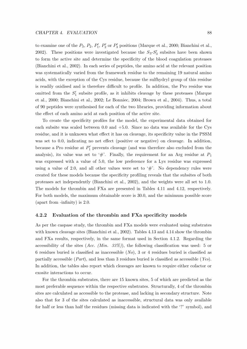
CHAPTER 4. EVALUATION 88
to examine one of the P3, P2, P ′
1, P ′
2 or P ′
3 positions (Marque et al., 2000; Bianchini et al.,
2002). These positions were investigated because the S3-S′
3 subsites have been shown
to form the active site and determine the specificity of the blood coagulation proteases
(Bianchini et al., 2002). In each series of peptides, the amino acid at the relevant position
was systematically varied from the framework residue to the remaining 19 natural amino
acids, with the exception of the Cys residue, because the sulfhydryl group of this residue
is readily oxidised and is therefore difficult to profile. In addition, the Pro residue was
omitted from the S ′
1 subsite profile, as it inhibits cleavage by these proteases (Marque
et al., 2000; Bianchini et al., 2002; Le Bonniec, 2004; Brown et al., 2004). Thus, a total
of 90 peptides were synthesised for each of the two libraries, providing information about
the effect of each amino acid at each position of the active site.
To create the specificity profiles for the model, the experimental data obtained for
each subsite was scaled between 0.0 and +5.0. Since no data was available for the Cys
residue, and it is unknown what effect it has on cleavage, its specificity value in the PSSM
was set to 0.0, indicating no net effect (positive or negative) on cleavage. In addition,
because a Pro residue at P ′
1 prevents cleavage (and was therefore also excluded from the
analysis), its value was set to ‘#’. Finally, the requirement for an Arg residue at P1
was expressed with a value of 5.0, the low preference for a Lys residue was expressed
using a value of 2.0, and all other values were set to ‘#’. No dependency rules were
created for these models because the specificity profiling reveals that the subsites of both
proteases act independently (Bianchini et al., 2002), and the weights were all set to 1.0.
The models for thrombin and FXa are presented in Tables 4.11 and 4.12, respectively.
For both models, the maximum obtainable score is 30.0, and the minimum possible score
(apart from -infinity) is 2.0.
4.2.2 Evaluation of the thrombin and FXa specificity models
As per the caspase study, the thrombin and FXa models were evaluated using substrates
with known cleavage sites (Bianchini et al., 2002). Tables 4.13 and 4.14 show the thrombin
and FXa results, respectively, in the same format used in Section 4.1.2. Regarding the
accessibility of the sites (Acc. (Min. 33%)), the following classification was used: 5 or
6 residues buried is classified as inaccessible (No), 3 or 4 residues buried is classified as
partially accessible (Part), and less than 3 residues buried is classified as accessible (Yes).
In addition, the tables also report which cleavages are known to require either cofactor or
exosite interactions to occur.
For the thrombin substrates, there are 15 known sites, 5 of which are predicted as the
most preferable sequence within the respective substrates. Structurally, 4 of the thrombin
sites are calculated as accessible to the protease, and lacking in secondary structure. Note
also that for 3 of the sites calculated as inaccessible, structural data was only available
for half or less than half the residues (missing data is indicated with the ‘?’ symbol), and

CHAPTER 4. EVALUATION 89
Subsites S3 S2 S1 S1’ S2’ S3’Weights 1 1 1 1 1 1
Gly 3.115 0.197 # 0.619 0.310 1.077Ala 3.771 0.540 # 0.714 0.786 1.539Val 3.361 0.829 # 0.033 0.857 1.000Leu 2.951 0.987 # 0.038 0.786 0.808Ile 3.689 0.697 # 0.029 0.786 0.846Pro 0.098 5.000 # # 0.141 1.192Phe 3.689 0.083 # 0.062 5.000 1.039Tyr 3.197 0.005 # 0.003 3.333 1.308Trp 2.213 0.008 # 0.001 1.643 2.039Ser 3.607 0.020 # 5.000 0.500 1.539Thr 4.508 0.072 # 0.476 0.476 0.846Cys 0.000 0.000 # 0.000 0.000 0.000Met 5.000 0.211 # 0.060 1.024 1.423Asn 2.623 0.016 # 0.021 0.476 1.500Gln 3.115 0.040 # 0.022 0.357 1.577Asp 0.533 2.632E-4 # 5.000E-4 0.008 0.096Glu 1.721 0.001 # 2.024E-4 0.015 0.127Lys 2.705 0.116 2.000 6.191E-4 0.691 3.154Arg 4.262 0.003 5.000 0.008 1.310 5.000His 3.607 0.018 # 0.045 0.595 1.692
Table 4.11: Thrombin PoPS specificity model.
Subsites S3 S2 S1 S1’ S2’ S3’Weights 1 1 1 1 1 1
Gly 5.000 4.039 # 1.750 3.654 4.333Ala 3.269 0.769 # 3.654 3.077 3.000Val 3.846 0.327 # 1.500 2.885 1.250Leu 3.077 0.500 # 0.596 5.000 1.200Ile 2.308 0.160 # 0.635 3.462 1.500Pro 2.500 0.981 # # 0.269 2.333Phe 3.269 5.000 # 0.615 3.462 1.350Tyr 1.154 1.423 # 0.712 3.462 1.667Trp 3.654 2.308 # 0.192 2.308 0.883Ser 2.500 0.365 # 5.000 2.692 5.000Thr 2.692 0.212 # 2.885 2.308 4.333Cys 0.000 0.000 # 0.000 0.000 0.000Met 2.692 0.142 # 0.462 0.789 3.000Asn 3.077 0.212 # 1.115 2.115 4.333Gln 5.000 0.289 # 0.500 1.289 2.667Asp 0.885 0.017 # 0.462 1.558 4.167Glu 2.115 0.231 # 0.165 1.558 2.833Lys 2.500 0.075 2.000 0.365 1.173 3.333Arg 3.654 0.327 5.000 0.500 1.654 3.000His 4.808 0.231 # 1.115 1.635 4.833
Table 4.12: FXa PoPS specificity model.

CHAPTER 4. EVALUATION 90
Site Acc. 2 2
Cleavage Max. Score/ (Min. Struct. Struct. PossibleSubstrate Site Score Rank 33%) DSSP PSIPRED PEST
SPR.SFQ+ 25.18/1 Yes S CCCCCC SP GoodFVIII1 EPR.SFS 25.18 23.26/2 - - CCCCCC None
QIR.SVA 16.21/9 Yes E HHHHHH QI PoorGIR.SFR+ 23.81/1 - - HHHHHC P ′
3 R PoorFV2 SPR.TFH 23.81 20.78/3 - - CCCCCC None
YLR.SNN 16.16/8 No ???? CCCCCC YL InvalidPAR-13 DPR.SFL+ 21.34 21.34/1 No SSS CHHHHC None
CLR.SFQ 17.56/1 - - SCCCCC RSFQ InvalidProtein S
DLR.SCV17.56
12.52/9 - - CCCCCC RSCV InvalidATIII4 AGR.SLN 17.22 16.25/2 No S B SCCCCC AG InvalidFg-B5 SAR.GHR+ 15.94 15.36/2 Yes CCCCCC SA InvalidFg-A6 GVR.GPR+ 18.40 14.70/5 Yes CCCCCC GV InvalidFXI7 KPR.IVG∗ 18.46 14.67/5 No ??? BS CCCSSC None
Protein C DPR.LID∗ 15.75 11.45/10 No ??? BS CCSSSC DP GoodPlasminogen PGR.VVG 16.80 7.26/57 No BS CCCSSC None
Table 4.13: Results for the thrombin specificity model over known thrombin cleavage sites.+Requires exosite interactions; ∗Requires cofactor; 1Coagulation factor VIII; 2Coagulation fac-tor V; 3Protease-activated receptor 1; 4Antithrombin; 5Fibrinogen B chain; 6Fibrinogen A chain;7Coagulation factor XI.
PSIPRED predicted these sites as not having significant secondary structure. Further-
more, in the case of the ATIII cleavage site, the second and fourth structures returned
indicated that the site had no regular secondary structure, and was accessible to the pro-
tease. The analysis of PEST regions showed that where PEST regions were predicted to
occur across the cleavage sites, they terminated at the P1 Arg residue. However, there did
not seem to be any consistent pattern regarding the occurrence of PEST regions across
the cleavage sites.
In general, the preferences exhibited by the thrombin active site reflect the preferences
for the natural substrates. In particular, the most catalytically favourable thrombin cleav-
age is the SPR.SFQ site in FVIII (Bianchini et al., 2002), which is predicted by PoPS to
have the highest score and a ranking of 1, while the least favourable thrombin cleavage is
the PGR.VVG site of plasminogen (Bianchini et al., 2002), which has a score of only 7.26
and a rank of 57. Additionally, the GIR.SIR and SPR.TFH sites in FV both obtained
higher scores than the YLR.SNN site, an observation which is consistent with the experi-
mental data which shows that these first two sites are catalytically more favourable than
the YLR.SNN site, even though this third site is the most important for fully activated
FV (Steen and Dahlback, 2002).
Some of the less successful predictions may be explained by alternative interactions.
Fibrinogen A chain cleavage requires exosite interactions, while cleavage of both FXI and
Protein C require a cofactor. However, this doesn’t explain the poor score and rank for the

CHAPTER 4. EVALUATION 91
Site Acc. 2 2
Cleavage Max. Score/ (Min. Struct. Struct. PossibleSubstrate Site Score Rank 33%) DSSP PSIPRED PESTATIII1 AGR.SLN 26.64 26.64/1 No S B SCCCCC AG Invalid
EPR.SFS 21.56/3 - - CCCCCC NoneQIR.SVA 21.04/7 Yes E HHHHHH QI Poor
FVIII2 SPR.SFQ 25.22 19.61/11 Yes S CCCCCC SP GoodRNR.AQS 18.81/14 Part HT HHHHHC NoneVPK.SFP 17.62/26 Part TS BSS CCCCCC KSFP InvalidGIR.SFR 21.62/4 - - HHHHHC P ′
3 R PoorSPR.TFH 19.66/12 - - CCCCCC None
FV3
YLR.SNN24.0
18.1/28 No ???? CCCCCC YL InvalidSWR.LTS 17.71/31 Part G TT CCCCCC None
PAR-24 KGR.SLI 23.04 23.04/1 - - CHHHHH NoneEGR.TAT 21.45/2 No T ???? CCCCCC RTAT Poor
ProthrombinDGR.IVE
21.8916.28/20 Part SS CCCSSC RIVE Poor
FVII5 QGR.IVG 21.89 21.89/1 No ??? BS CCSSSC NoneProtein S AAR.QST 21.4 16.56/12 - - CCCCCC AA invalidTFPI6 ICR.GYI 19.65 14.02/8 No SB E CCCCCS IC Invalid
QL PoorFVIIIi7 QLR.MKN 25.22 16.47/47 No ????? CCCCCC
KN Invalid
Table 4.14: Results for the FXa specificity model over known FXa cleavage sites. ∗Requirescofactor; 1Antithrombin; 2Coagulation factor VIII; 3Coagulation factor V; 4Protease-activatedreceptor 2; 5Coagulation factor VII; 6Tissue factor pathway inhibitor; 7Coagulation factor VIIIinhibitory site.
DLR.SCV cleavage of Protein S, or the lowest score and rank obtained for the plasminogen
cleavage, which on the basis of primary structure and the available specificity data, appears
to be a surprisingly unfavourable cleavage site. It should be noted that both Protein S
cleavage sites contain cysteine, which was not profiled and therefore was set to 0.0 in the
PSSM. This may have negatively influenced the prediction for these sites. It should also
be noted that two of the sites that require exosite interactions, SPR.SFQ of FVIII and
GIR.SFR of FV already have high scores and the highest rank.
The FXa model appeared to be less successful, particularly with respect to the rank-
ings of the sites. Furthermore, the specificity exhibited by the subsites was not always
consistent with the preference of FXa for its substrates. Of the 17 known cleavages, only
three were ranked as the top sites. One of these, the antithrombin cleavage site, is known
to be favourable to FXa (Bianchini et al., 2002). Other cleavages that are also relatively
favourable to FXa (Bianchini et al., 2002) and obtained reasonably high scores and rank-
ings are the PAR-2 and FVII cleavages, the EGR.TAT site of prothrombin, the EPR.SFS
cleavage of FVIII and the GIR.SFR cleavage site of FV. However, the TFPI cleavage site
and the DGR.IVE site of prothrombin are also favourable to FXa, yet neither of these sites
obtained good scores or rankings. The poor prediction of the prothrombin site might be
explained by the cofactor requirement for this cleavage, and in the case of TFPI a lack of

CHAPTER 4. EVALUATION 92
data for the Cys residue may have underestimated the preference for this site. Another site
with low score and rank is the Protein S AAR.QST site, which is possibly also explained
by the requirement for cofactor. Further, in the case of the VPK.SFP site of FVIII, the
low score and rank are immediately explained by the much less favoured Lys residue at the
P1 position. However, there are still a number of surprisingly low scores and/or rankings
for FV and FVIII (including the FVIII inhibitory site), all of which contain the highly
preferred Arg residue at P1.
With respect to structure, six of the FXa sites are predicted as at least partially
accessible to the active site. Furthermore, with the exception of the ATIII site AGR.SLN,
structural data was missing for all the inaccessible sites. For the ATIII site, the second
and fourth structures returned indicate that the site is accessible and has no secondary
structure, while and the fifth structure indicates that the site is partially accessible with
no secondary structure.
As in the case of the thrombin substrates, when a PEST region occurs across the active
site, it often terminates at the P1 Arg residue. Additionally, for FXa there are also a couple
of PEST sequences that begin at the P1 Arg residue, and invalid PEST regions that end
at the P1 Lys residue (FVIII VPK.SFP site), or the P ′
2 Lys residue (FVIIIi QLR.MKN
site). Thus, for both proteases there does not appear to be any noticeable pattern for the
occurrence of PEST regions across thrombin or FXa cleavage sites.
4.2.3 Comparing and measuring the thrombin and FXa models using
ROC curves
ROC curves were generated for both the thrombin and FXa models using the known
substrates listed in Tables 4.13 and 4.14, respectively. As in the caspase case study, the
known cleavage sites listed in the tables were used as true positives, and every other site
with an Arg or Lys residue at P1 was considered a true negative, consistent with the models
for each protease described in Section 4.2.1. The resulting curves are shown in Figure 4.13.
It is interesting to note that the summary tables of Section 4.2.2 suggested that the model
for FXa did not perform as well for the known FXa substrates as the thrombin model
did for the known thrombin substrates. However, both ROC curves have an area of 0.91,
indicating not only a high degree of accuracy and specificity for the respective substrates,
but also comparable performance for the two models.
For comparison, the thrombin and FXa models from PeptideCutter were also used to
predict the cleavage of the respective known substrates, and the ROC curves (generated
using the same true positive/true negative classification) are shown in Figure 4.13. As in
the case of the caspases, it is clear that the PoPS specificity models show much greater
specificity and sensitivity compared with the pattern-matching models of PeptideCutter.
Again, Cutter could not be compared with PoPS because it does not provide models
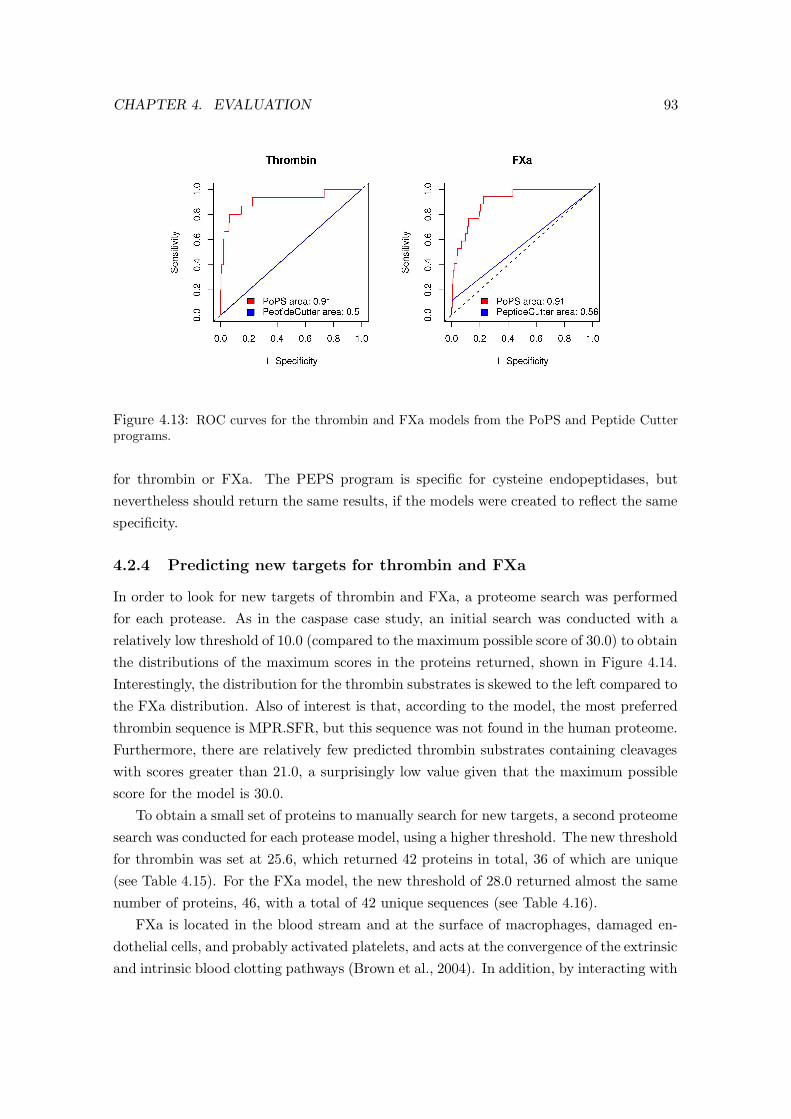
CHAPTER 4. EVALUATION 93
Figure 4.13: ROC curves for the thrombin and FXa models from the PoPS and Peptide Cutterprograms.
for thrombin or FXa. The PEPS program is specific for cysteine endopeptidases, but
nevertheless should return the same results, if the models were created to reflect the same
specificity.
4.2.4 Predicting new targets for thrombin and FXa
In order to look for new targets of thrombin and FXa, a proteome search was performed
for each protease. As in the caspase case study, an initial search was conducted with a
relatively low threshold of 10.0 (compared to the maximum possible score of 30.0) to obtain
the distributions of the maximum scores in the proteins returned, shown in Figure 4.14.
Interestingly, the distribution for the thrombin substrates is skewed to the left compared to
the FXa distribution. Also of interest is that, according to the model, the most preferred
thrombin sequence is MPR.SFR, but this sequence was not found in the human proteome.
Furthermore, there are relatively few predicted thrombin substrates containing cleavages
with scores greater than 21.0, a surprisingly low value given that the maximum possible
score for the model is 30.0.
To obtain a small set of proteins to manually search for new targets, a second proteome
search was conducted for each protease model, using a higher threshold. The new threshold
for thrombin was set at 25.6, which returned 42 proteins in total, 36 of which are unique
(see Table 4.15). For the FXa model, the new threshold of 28.0 returned almost the same
number of proteins, 46, with a total of 42 unique sequences (see Table 4.16).
FXa is located in the blood stream and at the surface of macrophages, damaged en-
dothelial cells, and probably activated platelets, and acts at the convergence of the extrinsic
and intrinsic blood clotting pathways (Brown et al., 2004). In addition, by interacting with

CHAPTER 4. EVALUATION 94
A
B
Figure 4.14: Histograms of the human proteome analysis for thrombin (A), and FXa (B), showingthe distribution of the maximum scores for the proteins returned, with the threshold score set to10.0 and no structural/score limits selected.

CHAPTER 4. EVALUATION 95
signalling receptors on the surface of a variety of cells, FXa is able to mediate a variety
of responses such as cell activation, gene expression and mitogenesis (Brown et al., 2004;
Ruf et al., 2003). Thrombin is also located in the circulating plasma, at the surface of
cells such as platelets and on endothelial cells at the site of vascular injury (Grand et al.,
1996; Brown et al., 2004). In addition to acting as the last protease in the blood clotting
cascade, thrombin can elicit mitogenic responses from a variety of cells, regulate neurite
growth and initiate the resorption of bone (Grand et al., 1996; Brown et al., 2004).
As in the caspase study, the NCBI (http://www.ncbi.nlm.nih.gov/) and Swiss-Prot
(http://us.expasy.org/sprot/) databases were used to assess the likelihood of each pre-
dicted target being a substrate, and the Pfam database
(http://www.sanger.ac.uk/Software/Pfam/) was used to find any interesting domains.
Unless a specific reference is made, the details in the remainder of this section come from
these sources. Predicted targets with an appropriate functional role were further assessed
for accessibility and structure using PoPS, and the notations used to describe features of
the cleavage sites (consensus site, secondary structure, accessibility and potential PEST
regions) follows that defined in previous sections of this chapter.
From the thrombin analysis (see Table 4.15) there were two particularly interesting re-
sults. The first of these is the Signal peptide, CUB domain, EGF-like 3 protein (SCUBE3),
which has been recently identified in primary osteoblasts, the humerus and femur bones,
in human umbilical vein endothelial cells and in the heart (Wu et al., 2004). SCUBE3 is
a secreted glycoprotein that can form oligomers tethered at the cell-surface of osteoblasts,
and appears to play an important role in bone cell biology (Wu et al., 2004), and therefore
is of interest due to thrombin’s role in bone morphology. The predicted site, TPR.SYK,
has a score of 26.0 and is predicted by DSSP to be in a partially accessible site. The
secondary structure obtained from DSSP is TT , while the secondary structure pre-
dicted by PSIPRED is CCCCCS. The site is not located within a PEST region. SCUBE3
appears to be processed by a serum-associated protease, but the identified site occurs at
the KGR.RAR sequence at residues 535-540 (Wu et al., 2004). Using PoPS, it can be seen
that this site is located in a short region of approximately 20 amino acids that is enriched
for 8 low preference sites. There is no known structure for this region, but it is predicted
by PSIPRED to be unstructured, and PESTfind reports no PEST region. Using the Pfam
database, it is noted that the predicted TPR.SYK site is located in an N-terminal EGF do-
main. Many EGF proteins require calcium for biological function, and a calcium-binding
site is located in the N-terminus of some EGF-like domains, e.g. in human coagulation
factor XI. In SCUBE3, the EGF domain occurs from residues 29-68, therefore cleavage
of the TPR.SYK sequence between residues 51-52 would remove the calcium-binding site.
Furthermore, it is possible that SCUBE3 may interact with the SCUBE1 protein located
in blood-vessel endothelial cells (Wu et al., 2004).

CHAPTER 4. EVALUATION 96
NCBI PoPSAccession Substrate Description Score
NP 003322.2 Tyrosine kinase 2 28.7NP 031394.2 RAS p21 protein activator 3 28.7NP 689963.2 Hypothetical protein FLJ23834 28.6XP 379182.1 Hypothetical protein XP 379182 28.6NP 115866.1 Mitochondrial ribosomal protein L41 28.1XP 373836.1 Hypothetical protein XP 378850 28.1NP 056036.1 Dynamin binding protein 27.8NP 065973.2 Protein kinase, lysine deficient 3 27.4NP 003094.4NP 115571.1NP 478063.2 SON DNA-binding protein 27.1NP 620304.1NP 620305.1XP 376532.1 Similar to KIAA0408 protein 26.9NP 689570.1 Zinc finger protein 440 26.9XP 376479.2 Mediator of DNA damage checkpoint 1 26.5NP 000332.1 Solute carrier family 3, member 1 26.4NP 005349.3 LIM domain only 7 26.3NP 005535.1 Insulin receptor substrate 1 26.1NP 689966.2 Signal peptide, CUB domain, EGF-like 3 26.0NP 006339.2NP 859422.1
Component of oligomeric golgi complex 5 26.0
NP 079426.2NP 689508.3
Threonyl-tRNA synthetase 25.9
NP 689547.2 FLJ25005 protein 25.9NP 003763.2 Jerky homolog-like 25.9NP 004179.2 Growth factor independent 1B 25.8NP 663632.1 Homeobox protein Gsh-1 25.8NP 005254.1 Growth factor independent 1 25.8XP 370995.1 Snail homolog 3 25.8NP 149120.1 Scratch 2 protein 25.8NP 112599.1 Scratch 25.8NP 005976.2 Snail 1 homolog 25.8NP 003059.1 Snail 2 25.8NP 079120.1 Pericentrin 1 25.8NP 000140.1 Fucosyltransferase III 25.8NP 002025.2 Fucosyltransferase V 25.8NP 000141.1 Fucosyltransferase VI 25.8NP 060549.3 Hypothetical protein FLJ10379 25.8NP 006260.1 Retinitis pigmentosa RP1 protein 25.8NP 060592.2 Hypothetical protein FLJ10514 25.7NP 612147.1 Rap2-binding protein 9 25.7
Table 4.15: The top scoring targets for thrombin from the human proteome analysis.

CHAPTER 4. EVALUATION 97
The second interesting result is the closely related family of glycosyltransferases called
the fucosyltransferases (FucTs), comprising FucT-III, FucT-V and FucT-VI (Table 4.16).
These proteins have similar catalytic function, however, they appear to have different
physiological functions (Grabenhorst et al., 1998; Borsig et al., 1998). They are respon-
sible for surface glycosylation of endothelial cells which is important to a number of pro-
cesses including coagulation, inflammation, metastasis and lymphocyte homing (Schnyder-
Candrian et al., 2000), and all three FucTs have been found at the cell surface (Borsig
et al., 1996; Costa et al., 1997; Borsig et al., 1998). In addition, FucT-III and VI are se-
creted in significant quantities (Grabenhorst et al., 1998), with FucT-VI constituting the
majority of human plasma α1,3-fucosyltransferase activity (Borsig et al., 1998). FucT-VI
originates from the liver, and from Weibel-Palade bodies located in vascular endothelial
cells which fuse with the plasma membrane to release their contents into the circulating
blood (Borsig et al., 1998; Schnyder-Candrian et al., 2000; van Mourik et al., 2002). All
three FucTs are predicted to be cleaved at the sequence RPR.SFS with a score of 25.8, and
in all cases the site is located in a region with no PEST sequence. There are no structures
for the FucTs, but FucT-VI is predicted to be unstructured (CCCCCC), while FucT-III
and V have predicted secondary structures of CCCHHH.
The proteome analysis for FXa (see Table 4.16) also contained two predictions of
particular interest. The first of these is Phosphodiesterase 4A (PDE4A), which is found in
the granules of two types of granulocytes, eosinophils and neutrophils, and is localised to
the extracellular space on release of the granules (Pryzwansky and Madden, 2003). PDE4A
belongs to the family of phosphodiesterases which can regulate cyclic AMP (cAMP),
a key second messenger that appears to be able to regulate protein kinase A (PKA),
which in turn can regulate serum adhesion proteins through phosphorylation (Pryzwansky
and Madden, 2003). Through these sequence of events, PDE4A release may be able to
regulate cell-cell interaction at sites of inflammation by degrading cAMP and therefore
downregulating PKA activity (Pryzwansky and Madden, 2003). The predicted cleavage
site occurs at the sequence GGR.SLT, with a score of 28.4, with only the two glycines
determined as highly accessible. The secondary structure obtained from DSSP is TS HHH,
while the secondary structure predicted from PSIPRED is CCCCHH, and the site is
located in an invalid PEST region.
The second interesting target for FXa is the acyl-CoA synthetase long-chain family
member 6, first identified as LACS5 (Malhotra et al., 1999). Long-chain acyl-CoA syn-
thetase (LACS) has a key role in erythrocyte membrane fatty acyl metabolism (Malhotra
et al., 1999). LACS5 is very different from other human acyl-CoA synthetases. It is highly
expressed in erythrocyte precursors and human brain, but is virtually absent from other
tissues, and it is possibly this form of LACS that is responsible for remodelling of the
plasma membrane lipids and proteins (Malhotra et al., 1999). The predicted cleavage site

CHAPTER 4. EVALUATION 98
NCBI PoPSAccession Substrate Description Score
NP 003770.1 β-N-acetylglucosaminyl-glycolipid β-1,4-galactosyltransferase 3 30.0NP 006715.1NP 005913.1
MAPK/ERK kinase kinase 4 30.0
NP 060123.2 Dymeclin 29.8XP 166479.2 KIAA0240 29.8XP 376178.1 Thyroid hormone receptor interactor 12 29.3NP 853630.1 Keratin associated protein 13-1 29.3XP 375207.1 Similar to RIKEN cDNA 1110004B15 29.1NP 848650.2 Hypothetical protein FLJ25770 29.1NP 976307.1 Hypothetical protein LOC283807 29.1NP 258261.2 ATP-binding cassette, sub-family C, member 10 29.0NP 002936.1 Replication protein A1 (70kD) 29.0NP 036207.1 Conserved gene telomeric to alpha globin cluster 29.0NP 065073.2 KIAA1244 29.0NP 002487.1 NADH dehydrogenase (ubiquinone) Fe-S protein 8, 23kDa 28.9NP 997337.1 FLJ44815 protein 28.9NP 694998.1 Hypothetical protein MGC33486 28.9XP 039877.8 Mucin 5, subtype B, tracheobronchial 28.9NP 072174.2 Tensin 28.7NP 057174.1 RNA binding motif protein 7 28.7XP 377742.1 KIAA1940 protein 28.7XP 290502.2 KIAA1030 protein 28.7NP 955523.1NP 955522.1
Talanin 28.7
XP 115769.2 Similar to chromosome 20 open reading frame 81 28.5NP 002396.2 Manic fringe homolog 28.5NP 542387.1 Hypothetical protein MGC13017 28.5NP 006193.1 Phosphodiesterase 4A, cAMP-specific 28.4NP 065172.1 Calcium/calmodulin-dependent protein kinase IG 28.4NP 859063.2 Hypothetical protein LOC163782 28.4NP 112599.1 Scratch 28.4NP 078950.1 RNA-binding protein LIN-28 28.3NP 001973.1 v-erb-b2 erythroblastic leukemia viral oncogene homolog 3 28.3NP 899228.2 Hypothetical protein LOC200030 28.3XP 371842.1 Hypothetical protein XP 376524 28.3NP 003658.1 G protein-coupled receptor 49 28.3NP 056071.1 Acyl-CoA synthetase long-chain family member 6 28.3NP 004570.2 Mitogen-activated protein kinase kinase kinase kinase 2 28.2NP 112197.1 TSC-22-like 28.2NP 620135.1 Synaptotagmin-like 5 28.1NP 004953.1 Growth differentiation factor 10 precursor 28.1NP 057323.2 Myosin XV 28.1XP 377951.1XP 380015.1
Similar to peptidylprolyl isomerase A 28.1
NP 004940.1NP 077740.1
Desmocollin-3 28.0
Table 4.16: The top scoring targets for FXa from the human proteome analysis.

CHAPTER 4. EVALUATION 99
is FFR.SLS, located in an invalid PEST region. There are no available structures, but the
predicted secondary structure from PSIPRED is HHHCCC.
A key issue in the proteome analyses for these two proteases, however, is that the ma-
jority of the predicted targets are not located in blood, and many are not even extracellular
proteins, and therefore they would be unlikely to ever come into contact with either FXa
or thrombin. This highlights an important future improvement to the proteome search,
which is to classify the proteins in the proteome database, for example by gene ontology
(GO) terms, to enable screening according to structure, function and localisation of the
putative targets.
4.3 Case study 3: MT1-MMP
This case study focuses on the specificity of the metallo protease membrane type-1 matrix
metalloproteinase (MT1-MMP). This protease degrades extracellular, cell-surface and sig-
nalling proteins, and is known for remodelling the extracellular matrix and for regulating
cell growth. In addition, high levels of MT1-MMP expression have also been associated
with aggressive cancers, which is not explained by cleavage of these substrates. Instead,
evidence suggests that MT1-MMP might cleave proteins of the centrosome, a cellular
structure which regulates the microtubule cytoskeleton and is therefore central to cell
division. This possible link between MT1-MMP and the centrosome could explain the
association between MT1-MMP and aggressive cancers. The following sections describe
how PoPS was used to investigate specificity of MT1-MMP for proteins of the centrosome,
and how the centrosomal protein pericentrin was identified as a potential new MT1-MMP
target.
4.3.1 The role of MT1-MMP
The matrix metalloproteinases (MMPs) are a family of related proteins that can be seg-
regated into two groups, soluble or membrane-bound (Sternlicht and Werb, 2001; Kridel
et al., 2002; Das et al., 2003). Their name derives from their potent ability to degrade
the proteins of the extracellular matrix, together with their dependence on zinc for cat-
alytic activity (Sternlicht and Werb, 2001; Das et al., 2003; Lessner and Galis, 2004). In
addition to cleaving matrix proteins, it has become clear that the MMPs are also capable
of cleaving cell surface proteins and pericellular non-matrix proteins, regulating a diverse
array of essential functions, including regulation of cell signalling and behaviour, bone
development, vascular remodelling and angiogenesis. Furthermore, the MMPs also play a
role in a number of pathologies including arthritis and cancer (Sternlicht and Werb, 2001;
Mott and Werb, 2004).
The membrane-bound MMPs are known as the membrane type-matrix metallopro-
teinases (MT-MMPs). Compared with the secreted MMPs, the membrane-anchored MMPs

CHAPTER 4. EVALUATION 100
have alternative cellular localisation, different substrate targets, an unusual interaction
with the tissue inhibitors of metalloproteinases (TIMPS), and unusual mechanisms of reg-
ulation involving internalisation, processing and ectodomain shedding (Osenkowski et al.,
2004). The prototypic member of the MT-MMPs is the membrane type-1 matrix metal-
loproteinase (MT1-MMP), also known as MMP14, which is associated with a variety of
cellular and developmental processes and a number of pathological conditions (Sternlicht
and Werb, 2001; Kridel et al., 2002; Itoh and Seiki, 2004). So far, MT1-MMP is the
only MMP identified as essential for survival, with the loss of this enzyme causing pro-
gressive impairment of postnatal growth and development, affecting the skeleton and soft
connective tissues (Osenkowski et al., 2004; Holmbeck et al., 2004). MT1-MMP degrades
proteins of the extracellular matrix, as well as cell surface and signalling proteins, thereby
regulating several cellular functions including extracellular matrix turnover, cell growth,
and promotion of cell migration and invasion (Sternlicht and Werb, 2001; Seiki et al., 2003;
Itoh and Seiki, 2004; Tam et al., 2004; Osenkowski et al., 2004). In particular, MT1-MMP
is associated with aggressive, invasive malignancies (Egeblad and Werb, 2002). However,
the pericellular functions of MT1-MMP do not fully explain the roles of MT1-MMP in
either normal development or malignancies (Golubkov et al., 2005).
MT1-MMP has been shown to have a high trafficking rate in colon carcinoma cells,
which is sensitive to the inhibitor of tubulin polymerisation, nocodazole (Deryugina et al.,
2004). More recently, large fractions of MT1-MMP have been shown to be located at
the plasma membrane (cell surface) and in multiple intracellular vesicles, while a smaller
fraction accumulates at centrosomes, particularly in dividing metaphase cells (Golubkov
et al., 2005). In addition, active MT1-MMP has been found to associate with γ-tubulin,
an important component of the microtubulin cytoskeleton, which is responsible for rapid
protein trafficking between the nucleus and plasma membrane (cell surface) (Golubkov
et al., 2005). This association is not surprising, since the centrosome is the microtubule-
organising centre, and is vital to regulation of the mitotic spindle and separation of the
sister chromatids during cell division (Nasmyth, 2002). These data suggest that MT1-
MMP associates with the centrosome during metaphase, and as it is proteolytically po-
tent, possibly cleaves centrosomal proteins, which may explain its role in tumorigenesis
(Golubkov et al., 2005). With this in mind, PoPS was used to investigate the specificity
of MT1-MMP for centrosomal targets.
4.3.2 Developing specificity models for MT1-MMP
The specificity of MT1-MMP has been profiled using substrate phage display (Kridel
et al., 2002). This analysis revealed the interesting dual specificity exhibited by MT1-
MMP. The first mode of specificity was a preference for non-selective substrates that were
also cleaved by MMP-2 and MMP-9, while the second mode was for substrates selective
for MT1-MMP alone. The difference between the two modes is that in the non-selective

CHAPTER 4. EVALUATION 101
mode, the substrates prefer collagen-like cleavage motifs that contain a Pro residue at P3,
and use the contacts of the P3 and P ′
1 positions to bind and cleave substrates. In contrast,
Pro residues are absent from the selective substrates, and MT1-MMP instead appears to
select for an Arg residue at P4, using the P4 and P ′
1 contacts during cleavage.
To investigate the potential role of the Arg-specific (selective) binding mode in the
recognition of centrosomal proteins, a PoPS model was created for the specific binding
mode. Using expert knowledge derived from the phage data, Jeffrey Smith and Andrei
Osterman (The Burnham Institute, La Jolla, San Diego, U.S.A) used a conventional set
of features including size, charge and polarity to construct the position specific scor-
ing matrix. This model is available from the PoPS models database with the identifier
M10.014>Osterman>1.1, and is referred to here as sel-MT1-MMP. For the non-specific
binding mode observed for MT1-MMP, a second model was created with the identifier
M10.014>Boyd>2.1, referred to here as ns-MT1-MMP. These two models are largely sim-
ilar (see Table 4.17), with a few specific differences to indicate the different binding modes
described above. The selective mode has the Arg residue in the S4 profile set to the
maximum possible score of 5.0, and does not accept a Pro residue at any position. In
addition, the values for the Gly and Ala residues in the S1 profile are relatively low (a
score of 1.0), as is the preference for the Ile residues in the S ′
1 profile (a score of 0.5). The
non-selective mode is indicated by an exclusion of the Arg residue from the S4 profile, and
a maximal preference (score of 5.0) for the Pro residue in the S3 profile. The score for the
Pro residue at all the other positions is 0.0. The values for the Gly and Ala residues in
the S1 profile and Ile in the S ′
1 profile are relatively high compared to the selective mode.
Finally, the weights have been chosen to reflect the observed importance of the subsites.
The differences in the weights reflect the altered importance of the S4 and S3 sites between
the two binding modes. The minimum score for both models is -4.0. The maximum score
for sel-MT1-MMP is 60.0, and for ns-MT1-MMP is 61.0.
4.3.3 Relevance of MT1-MMP binding modes to centrosomal substrates
As described in Section 4.3.1, it appears that MT1-MMP may cleave centrosomal targets,
and so the aim was to see if the selective binding mode, expressed by sel-MT1-MMP,
showed preference for centrosomal proteins over all other proteins in the human proteome.
In addition, it was interesting to see if any preference was also shown by the non-selective
binding mode (ns-MT1-MMP model) for centrosomal proteins over the human proteome,
and how this compared to the selective mode.
The centrosomal proteome, i.e. all the identified proteins that make up the human
centrosome, has been published (Andersen et al., 2003), and these sequences were obtained
from the Swiss-Prot database (http://us.expasy.org/sprot/) and collated into a fasta
file of 112 sequences. To allow comparison with the human proteome, the fasta file was then
screened to remove any proteins that were not present in the human proteome database,

CHAPTER 4. EVALUATION 102
Subsites S4 S3 S2 S1 S1’Weights 41/12 21/42 1 2 5
Gly # # 2.0 1.01/5.02 #Ala 3.0 2.0 1.0 1.01/3.02 #Val 2.0 3.0 0.0 -2.0 0.0Leu 1.0 4.0 3.0 -2.0 5.0Ile 0.0 2.0 0.0 0.0 0.51/3.02
Pro #1/0.02 #1/5.02 #1/0.02 #1/0.02 #1/0.02
Phe 0.0 0.0 1.0 1.0 0.5Tyr 0.0 3.0 1.0 -2.0 0.0Trp 0.0 0.0 0.0 1.0 0.0Ser 3.0 3.0 0.0 1.0 #Thr 1.0 1.0 0.0 0.0 #Cys 0.0 0.0 0.0 0.0 #Met 1.0 2.0 2.0 -2.0 0.5Asn 1.0 0.0 0.0 1.0 #Gln 2.0 2.0 1.0 0.0 #Asp 0.0 0.0 0.0 -2.0 #Glu 0.0 0.0 1.0 -2.0 #Lys 3.0 1.0 2.0 -2.0 #Arg 5.01/#2 2.0 1.0 -2.0 #His 1.0 1.0 1.0 2.0 #
Table 4.17: MT1-MMP models for the two different binding modes. 1 Selective mode, sel-MT1-MMP model; 2 Non-selective mode, ns-MT1-MMP model.
which is derived from the RefSeq database (see Chapter 3, Section 3.7). A total of 92
of the original 112 sequences were retained and saved to a new fasta file. Then, both of
the MT1-MMP specificity models were used to find targets in the centrosomal proteome,
using the batch predictions module described in Chapter 3, Section 3.7. The distributions
of maximum scores returned are shown in Figure 4.15. Based on these analyses, the lowest
maximum score for the sel-MT1-MMP model was 38.0, and for the ns-MT1-MMP model
was 40.0.
The next step was to determine the selectivity of each model for centrosomal proteins
by comparing the proportion of centrosomal proteins selected to the proportion of proteins
selected from the whole human proteome. Since all the proteins from the centrosome are
returned when a threshold of 38.0 is used for sel-MT1-MMP, and a threshold of 40.0 is
used for ns-MT1-MMP (and therefore a lower value cannot return any more proteins),
these respective thresholds were used as the cut-off for the human proteome analyses (see
Table 4.18), and the analysis was run using the standard proteome predictions module.
The first goal was to assess whether the two different binding modes show any dis-
crimination for the centrosomal proteins alone compared to the preference for proteins in
the entire human proteome. For each model, the results of the predicted hits from the
centrosome and the human proteome were compared on the basis of the proportion of
CHAPTER 4. EVALUATION 103
A
B
Figure 4.15: Histogram of the centrosomal proteome analysis for the two MT1-MMP models,sel-MT1-MMP (A) and ns-MT1-MMP (B), showing the distribution of the maximum scores forall the centrosome proteins, with no structural/score limits selected.

CHAPTER 4. EVALUATION 104
Number of Number of proteinsModel Protein set proteins Cut-off above cut-off
Centrosome 92 92sel-MT1-MMP
Human proteome 2797538.0
27244Centrosome 92 92
ns-MT1-MMPHuman proteome 27975
40.027327
Table 4.18: Input for the analyses of the centrosome and human proteome using the modelsns-MT1-MMP and sel-MT1-MMP.
substrates returned at a series of thresholds above the respective cut-offs (see Table 4.19).
These proportions are expressed as a percentage of the total number of proteins in the
data set. Then, for each threshold, the difference was calculated between the proportion
returned from the centrosome and the proportion from the human proteome, i.e.:
% centrosome targets above threshold - % human proteome targets above threshold
Both models appear to be enriched for centrosomal targets compared with the human
proteome, i.e. at higher scores a greater percentage of centrosomal proteins are returned
compared to the proportion of human proteome targets that are returned (indicated by
a positive value for the percentage difference). The question is whether the sel-MT1-
MMP model has a higher selectivity compared to the ns-MT1-MMP model. However, the
results in Table 4.19 cannot be compared directly because the scores for one model do not
translate directly into the same score for the other model (since the maximum scores for
the two models are not the same). To enable comparison of the models, the thresholds were
normalised between 0.0 and 10.0, and then the percentage differences shown in Table 4.19
sel-MT1-MMP Model ns-MT1-MMP Model% Proteins % Proteins % Proteins % Proteins
from from human from from humanThreshold centrosome proteome % Difference centrosome proteome % Difference
38.0 100.0 97.4 2.6 - - -40.0 98.9 95.6 3.3 100.0 97.7 2.342.0 97.8 92.4 5.4 97.8 95.6 2.244.0 94.6 87.1 7.5 95.7 91.6 4.146.0 92.4 78.6 13.8 91.3 84.7 6.648.0 81.5 65.4 16.1 79.4 73.9 5.550.0 69.6 50.9 18.7 71.7 59.1 12.652.0 50.0 35.8 14.2 59.8 41.7 18.154.0 29.4 21.2 8.2 38.0 26.6 11.456.0 17.4 8.6 8.8 18.5 13.9 4.658.0 5.4 1.6 3.8 4.4 5.6 -1.260.0 0.0 0.1 -0.1 0.0 1.1 -1.1
Table 4.19: MT1-MMP human proteome and centrosome analyses, showing the percentage ofproteins returned for each threshold above the cut-off for the respective model.

CHAPTER 4. EVALUATION 105
Figure 4.16: Percentage differences of the MT1-MMP predictions. This graph shows the differencein the percentage of proteins returned for the centrosome analysis compared to the human proteomeanalysis, at each normalised threshold.
were graphed against these normalised thresholds, as shown in Figure 4.16. The results
show that ns-MT1-MMP has slightly more selectivity for centrosomal proteins around
the normalised range of 8.8-9.1, but overall the sel-MT1-MMP model is more selective
for centrosomal proteins than the ns-MT1-MMP model. This is particularly true at the
highest scores (the scores more likely to indicate cleavage), around 9.4-9.7 in the normalised
range. Of course, it is possible that the non-selective mode of MT1-MMP could also be
responsible for cleavage of any centrosomal proteins. However, the results indicate that
sel-MT1-MMP is highly selective for centrosomal proteins. Therefore, the next step was
to look for potential MT1-MMP targets within the centrosomal proteome, based on this
selective mode.
4.3.4 Identification of a new MT1-MMP substrate
The original 112 proteins of the centrosomal proteome (published in Andersen et al. (2003),
and obtained from the Swiss-Prot database) were analysed with the sel-MT1-MMP model
using the batch predictions module. Table 4.20 contains the top-scoring hits from this
search.

CHAPTER 4. EVALUATION 106
Swiss-Prot/NCBI PoPSIdentifier Substrate Description Score
NP 009117.2 Centrosomal protein 2 58.0NP 055730.1 KIAA1074 protein 58.0NP 659436.1 hypothetical protein MGC20806 58.0
O95613 Pericentrin 2 58.0Q9UPN4 KIAA1118 protein [Fragment] 58.0Q9C0D2 KIAA1731 protein [Fragment] 58.0
NP 006188.2 Pericentriolar material 1 57.0NP 065194.1 Tubulin, gamma complex associated protein 6 57.0NP 055627.1 KARP-1-binding protein 57.0NP 055490.1 KIAA0445gene product 57.0
Q9P209 KIAA1519 protein [Fragment] 57.0Q9Y6R9 BC282485 1 [Fragment] 57.0
NP 060610.1 Hypothetical protein FLJ10565 57.0NP 005742.4 A-kinase anchor protein 9 isoform 2 56.0NP 001061.2 Tubulin, gamma 1 56.0NP 006650.1 Tubulin, gamma complex associated protein 2 56.0NP 001367.2 Dynein heavy chain, cytosolic 56.0
O94927 KIAA0841 protein [Fragment] 56.0NP 078824.2 Hypothetical protein FLJ23047 56.0
Table 4.20: The top scoring targets for MT1-MMP from the human proteome analysis.
Of these hits, the protein Pericentrin 2 was particularly interesting because it is very
important for the normal functioning of centrosomes. Silencing of pericentrin expression
interferes with the formation of the mitotic spindle and the localisation of γ-tubulin to the
centrosomes, which results in G2 cell-cycle arrest, mitotic spindle aberrations and chromo-
somal instability (Doxsey et al., 1994; Zimmerman et al., 2004). Pericentrin is predicted to
have a number of potential cleavage sites, and while there is no available structure for this
protein, predicted secondary structure suggests that these sites are cleavable. Thus, syn-
thetic peptides representing the predicted sites were constructed, and two of these peptides
were found to be highly susceptible to MT1-MMP cleavage (Golubkov et al., 2005). These
peptides represented the predicted cleavage sequences RLLG1156L, predicted with a score
of 58.0, and RVLG672L, predicted with a score of 56.0. Intracellular cleavage of pericentrin
was confirmed in breast carcinoma MCF7 and glioma U251 cells. Intact pericentrin has a
molecular weight of 220kDa, while in the U251 cells cleaved pericentrin is observed in both
200kDa and 150kDa forms, with both cleavages occurring in the N-terminal region of the
protein (Golubkov et al., 2005). These data suggest that the 150kDa fragment correlates
to the RLLG1156L cleavage site.
In a further experiment, Madin Darby Canine Kidney (MDCK) epithelial cells were
used to show that centrosomal activity of MT1-MMP can induce DNA aneuploidy (miss-
ing chromosomes or more copies than normal), and the severity of this effect is directly

CHAPTER 4. EVALUATION 107
dependent on the level of MT1-MMP expression (Golubkov et al., 2005). As discussed ear-
lier, the normal functioning of centrosomes is required during cell division. In particular,
the centrosome regulates the mitotic spindle and sister chromatid function, which is essen-
tial for viable genomic inheritance and cell division (Nasmyth, 2002). Immunofluorescent
staining of the cells revealed numerous aberrations of the mitotic spindle in metaphase,
explaining the genetic instability (aneuploidy) seen in the MDCK cells (Golubkov et al.,
2005). Thus, it is proposed that MT1-MMP cleaves pericentrin, thereby inducing chro-
mosomal instability, which in turn results in malignant transformation. The onset of
chromosomal instability is a major predictor of carcinogenesis, therefore the ability of
MT1-MMP to cleave pericentrin in cells could help explain the observed link between
MT1-MMP expression and aggressive tumours (Golubkov et al., 2005).
4.4 Discussion
The three case studies presented here illustrate how PoPS can be used to investigate
protease specificity and predict new targets. The examples show how both experimental
data (even from different sources) and expert knowledge can be used to create specificity
models. Given known cleavage sites, the accuracy of the model can be measured using
factors such as predicted score and ranking of the cleavage sites, and ROC curves. As
illustrated in the first two case studies, if the model appears to predict known cleavage
sites accurately, it is possible to then use the model to predict new targets. Using this
process, PoPS was able to positively identify HDAC7 as an in vitro target of caspase 8.
While further work is needed to verify the biological significance of this substrate, the case
study illustrates the process that can be followed from developing the model to predicting
and testing potential new substrates.
Obviously, not all predicted targets will prove to be real substrates. This could be a
result of structural inhibition of cleavage, such as appears to be the case with the pre-
dicted caspase 8 cleavage site in Rab9, and possibly also with the TRIM3 site. In addition,
other factors such as incompatible cell/tissue expression or sub-cellular localisation of the
protease and substrate may also prevent in vitro cleavage. For example, Retinoblastoma-
associated factor 600 was interesting as a predicted caspase 1 target (Section 4.1.4), how-
ever, it may turn out that this protein, like Retinoblastoma protein, is localised to the
nucleus, and therefore inaccessible to caspase 1, which appears to be localised to the plasma
membrane. In the case of thrombin and FXa, this problem of co-localisation was more
obvious, with most of the results returned from the proteome analysis being inaccessible
to these proteases. Despite this, there were still some very interesting targets returned
from the proteome analyses in both case studies.
The third case study took an entirely different approach to the first two. In this
case, experimental data had shown that the MT1-MMP exhibits two discrete modes of

CHAPTER 4. EVALUATION 108
specificity: one which is very similar to the specificity of other matrix metalloproteases,
and the other which has a unique, selective specificity. It has been hypothesised that
the selective specificity mode might allow MT1-MMP to specifically target centrosomal
proteins, which would explain the link between high MT1-MMP expression and aggressive
cancers. Two specificity models were developed, one for each binding mode, and used to
screen both the centrosomal proteome and the human proteome for likely targets. The
results showed that the selective mode of MT1-MMP does show significant discrimination
for centrosomal proteins. The model was then used to identify potential new targets
of MT1-MMP. One of the predicted targets, pericentrin 2, was particularly interesting
because of the presence of several predicted cleavage sites, and because of the essential role
that pericentrin plays in normal cell division. Cleavage of pericentrin by MT1-MMP was
demonstrated, and the experimental results provided evidence that this cleavage causes
chromosomal instability, explaining the observed link between MT1-MMP and aggressive
cancers.
All these results demonstrate that PoPS is a powerful tool that can allow researchers
to easily and rapidly investigate protease specificity, and predict new targets. The tool has
a wide range of functionality for researchers, and is flexible enough to handle a number of
different tasks, providing a valuable complement to protease research.
Chapter 5
General Discussion and Future
Work
5.1 Does PoPS work?
When PoPS was first proposed, there was some skepticism about whether the preferences
of a protease for the sequences of amino acids in substrates, i.e. sequence specificity, could
be applied to predicting protease specificity. However, the results of Chapter 4 clearly
demonstrate that this is possible. The PoPS model of specificity is able to express even
subtle effects of protease specificity, and together with the sliding window alignment, can
be used to investigate and predict protease specificity. This model greatly improves on
the pattern-matching approaches of the Cutter and PeptideCutter programs, by allowing
even complex specificity to be easily specified, and by allowing more accurate expression of
specificity. The PoPS model of specificity also improves on the matrix-based approaches
of the PEPS and PrediSi programs, because it allows the expression of cooperative effects
with the use of optional dependency rules.
The PoPS system itself provides a number of modules to enable the user to gain insight
into the specificity of a protease, to test and measure the accuracy of specificity models,
and to predict substrate cleavage on an individual or large scale. PoPS is more flexible
than the existing PEPS and PrediSi programs, because it allows the user to produce a
model for any protease, using any source of specificity data. It also improves on existing
work by providing structural information about the substrate, to assist in identifying likely
cleavage sites, and by providing a models database as a publicly accessible resource for the
central storage and access of protease specificity information. Thus, the PoPS program is
a powerful resource for investigating protease specificity.
In the case of the caspases, specificity models were derived using a combination of
results from positional scanning libraries and from fluorescence-quenched substrates. Se-
quence specificity appears to be highly significant for the specificity of these proteases,
109

CHAPTER 5. GENERAL DISCUSSION AND FUTURE WORK 110
so that if a preferred sequence is present and accessible within the substrate, then the
caspase will usually cleave it. This was supported by the data of Tables 4.4, 4.5 and 4.6,
which showed that PoPS generally obtains high scores for known caspase cleavage sites.
In addition, using data from sequence specificity, PoPS was also able to identify HDAC7
as a potential new caspase 8 target. Clearly, sequence specificity is not the only factor,
as there were known cleavage sites (for example, calpastatin and plectin) that did not
have high scores or rankings, and the predicted substrates Rab9 and TRIM3 had high
scores, but were not susceptible to caspase 8 cleavage. However, the results of this case
study suggest that sequence specificity plays a very important role in determining caspase
specificity overall.
In the case of MT1-MMP, expert knowledge was used to generate two specificity models
that reflected the two binding modes of this protease. PoPS was then used to demonstrate
that the selective binding mode of MT1-MMP is specific for centrosomal proteins, and
this information was in turn used to successfully identify pericentrin as an MT1-MMP
substrate.
In the case of the blood coagulation proteases thrombin and FXa, the specificity models
were derived from fluorescence-quenched substrates, and used to examine known cleavage
sites. The results suggest that the specificity of thrombin and FXa is not fully explained
on the basis of sequence specificity alone. While the known cleavage sites were ranked
relatively well within the respective substrate sequences (Tables 4.13 and 4.14), the actual
scores were quite low compared to the maximum scores for the model. FXa, in partic-
ular, has been shown to have very general specificity that is not selective for its natural
substrates (Bianchini et al., 2002). For example, the primary function of FXa is to cleave
prothrombin at two locations, EGR.TAT, which has a high score and a ranking of 2, and
DGR.IVE, which has a low score and a ranking of 20. Interestingly, FXa is unable to
cleave a synthetic peptide containing the DGR.IVE sequence, suggesting that the low
PoPS score for this sequence is correct, and that there is in fact some interaction in the
prothrombinase complex that allows FXa to cleave this sequence in vivo (Robert Pike,
Monash University, Melbourne, Australia: personal communication).
While the PoPS program is clearly a powerful tool, the results of Chapter 4 show
that PoPS does not always get the right answer. There could be several reasons for this.
One is that specificity data are not always accurate or complete, and this directly affects
the accuracy of the specificity model. Another reason is that while the PoPS model of
specificity is ultimately based on the primary sequence preferences (sequence specificity) of
the protease, the influence of primary sequence on protease specificity is expected to vary,
at least partly because of the different biological role(s) of each protease. For example, in
the case of the caspases, once the process of apoptosis is initiated, rapid activity of these
proteases may be preferable, to ensure the process of cell death occurs quickly, efficiently
and essentially irreversibly. Conversely, the blood coagulation proteases must be tightly

CHAPTER 5. GENERAL DISCUSSION AND FUTURE WORK 111
regulated to ensure that a blood clot is only formed for an appropriate time and at the
correct location.
Thus, in some cases, factors other than primary sequence must affect protease speci-
ficity. Since one major factor is the structure of the substrate, the PoPS system provides
structural information about substrates, to allow the user to determine whether the (po-
tential) cleavage site is in a conformation that the protease can access and cleave. Where
possible, this information is derived from known structures of proteins. Otherwise struc-
tural information is predicted.
By considering not only the primary sequence but also the structure of the substrate,
PoPS aims to give a wholistic view of protease specificity. However, as with any predictive
system, consideration must always be given to the source of the data being applied, as
discussed in the following sections.
5.2 Consideration of the specificity data
This thesis raises some important questions about specificity profiling, such as how much
data is required to produce an accurate model, and what that data really tells us about
the specificity of a protease.
As discussed in Chapter 1, different experimental techniques provide different infor-
mation about the specificity of the protease. For example, positional scanning libraries
(PSL) provide information about the preference for each amino acid at each position,
but they rely on the contributions at each subsite being independent (i.e. no cooperative
effects). Phage display could provide information about cooperative effects, but only if
enough phage are sequenced, which is usually not the case. Furthermore, phage display
provides information about positive selection, but not about negative selection. In other
approaches, individual peptides are synthesised in a structured library to investigate indi-
vidual effects on specificity. However, the size of the library can quickly become too large
to be feasible (in terms of the time and cost involved).
One possible solution is to a statistical approach to maximise the quantity of data
obtained from an experimental technique, while minimising the size of the library. Thus,
factorial design (Box et al., 1978) has been recently used to design a small library of
16 peptides to investigate the cooperative effects of the complement protease C1s (PoPS
project: unpublished data). This study revealed that C1s does exhibit cooperative effects,
allowing an informed decision to be made about further specificity profiling of this protease.
This two-phase approach to specificity profiling may prove to be very useful as a general
approach for all proteases. In the first phase, an initial screen would be used to establish
whether the protease appears to exhibit cooperative effects. If it does, then an approach
like phage display, which provides specificity information despite cooperative effects, could
be selected. Otherwise, an approach like PSL, which can provide a comprehensive analysis
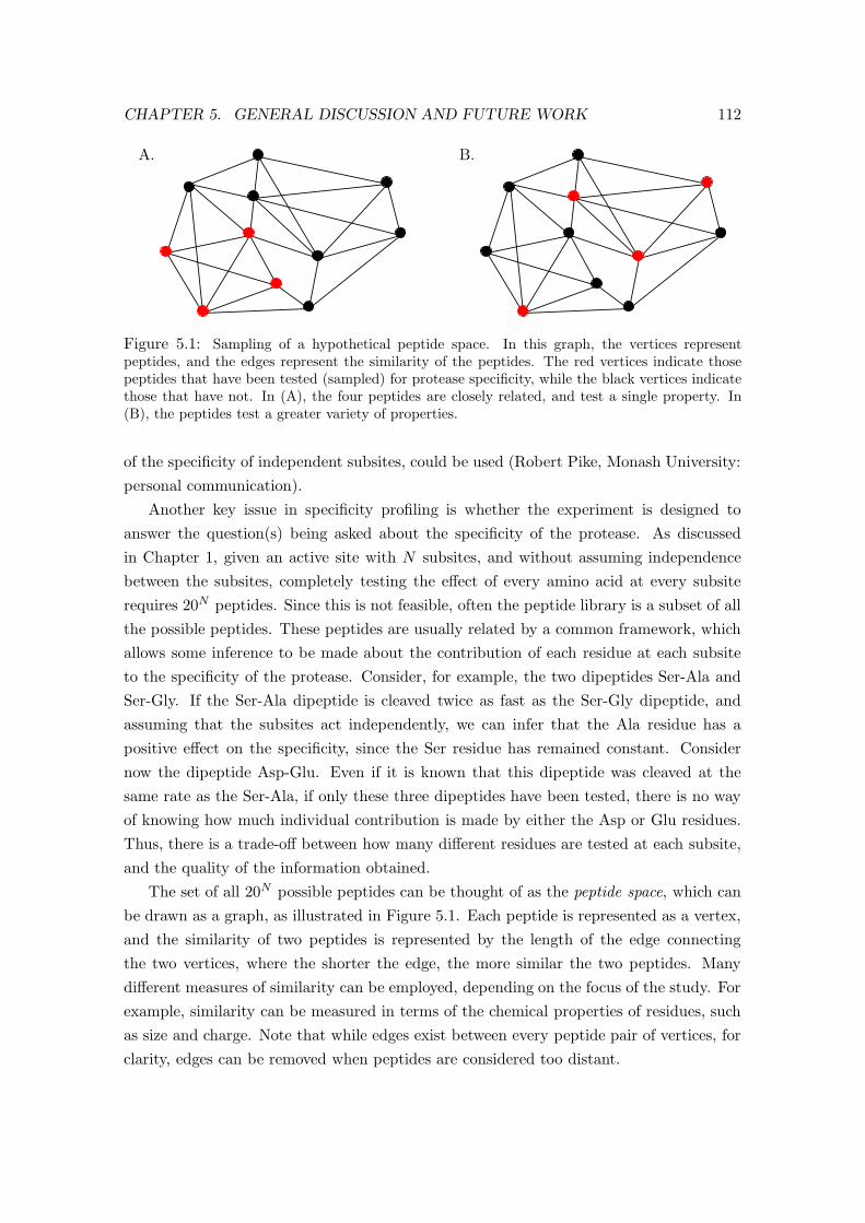
CHAPTER 5. GENERAL DISCUSSION AND FUTURE WORK 112
A.
3344
5566
7788
99::
;;<<
==>>
??@@
AABB
CCDD
EEFF
GGHH
B.
IIJJ
KKLL
MMNN
OOPP
QQRR
SSTT
UUVV
WWXX
YYZZ[[\
\
]]^^
Figure 5.1: Sampling of a hypothetical peptide space. In this graph, the vertices representpeptides, and the edges represent the similarity of the peptides. The red vertices indicate thosepeptides that have been tested (sampled) for protease specificity, while the black vertices indicatethose that have not. In (A), the four peptides are closely related, and test a single property. In(B), the peptides test a greater variety of properties.
of the specificity of independent subsites, could be used (Robert Pike, Monash University:
personal communication).
Another key issue in specificity profiling is whether the experiment is designed to
answer the question(s) being asked about the specificity of the protease. As discussed
in Chapter 1, given an active site with N subsites, and without assuming independence
between the subsites, completely testing the effect of every amino acid at every subsite
requires 20N peptides. Since this is not feasible, often the peptide library is a subset of all
the possible peptides. These peptides are usually related by a common framework, which
allows some inference to be made about the contribution of each residue at each subsite
to the specificity of the protease. Consider, for example, the two dipeptides Ser-Ala and
Ser-Gly. If the Ser-Ala dipeptide is cleaved twice as fast as the Ser-Gly dipeptide, and
assuming that the subsites act independently, we can infer that the Ala residue has a
positive effect on the specificity, since the Ser residue has remained constant. Consider
now the dipeptide Asp-Glu. Even if it is known that this dipeptide was cleaved at the
same rate as the Ser-Ala, if only these three dipeptides have been tested, there is no way
of knowing how much individual contribution is made by either the Asp or Glu residues.
Thus, there is a trade-off between how many different residues are tested at each subsite,
and the quality of the information obtained.
The set of all 20N possible peptides can be thought of as the peptide space, which can
be drawn as a graph, as illustrated in Figure 5.1. Each peptide is represented as a vertex,
and the similarity of two peptides is represented by the length of the edge connecting
the two vertices, where the shorter the edge, the more similar the two peptides. Many
different measures of similarity can be employed, depending on the focus of the study. For
example, similarity can be measured in terms of the chemical properties of residues, such
as size and charge. Note that while edges exist between every peptide pair of vertices, for
clarity, edges can be removed when peptides are considered too distant.

CHAPTER 5. GENERAL DISCUSSION AND FUTURE WORK 113
The size and structure of the peptide space can be altered by the goals of the specificity
study. For example, an experiment to test cooperativity between subsites will require a
different set of peptides to an experiment that assumes that the subsites act independently.
Alternatively, knowledge of restrictions on specificity can reduce the number of peptides
that need to be tested. For example, the caspase requirement for an Asp residue at
the P1 position results in the elimination of all peptides with any other residue at P1.
Nevertheless, the number of peptides required to be tested will generally still be too large
to be feasible. Therefore, careful planning of the library is required so that the peptides
provide as much specificity information as possible. This is illustrated in Figure 5.1. In
both (A) and (B), four peptides have been selected for testing, but while the peptides
in (A) are quite similar and thus could test a specific property, the peptides in (B) are
relatively distant and thus might be able to test a variety of properties. Note that in the
case of (B) in particular, it is necessary to ensure that enough peptides are sampled to
measure the individual contributions. Part of the future work will look at developing a
module to allow researchers to define and visualise the peptide space to be investigated,
and select a set of peptides from that space that will maximise the quantity and quality
of specificity data that is obtained. This will assist researchers in identifying how much
of the peptide space has already been sampled in any given experiment(s), as well as in
planning new experiments.
There is also a need to address those cases where the experimental data is limited. One
possible approach is to use classification methods on the specificity data. For example,
using common properties of the amino acids, such as size or charge, the residues that are
selected at each subsites can be classified into groups, which can in turn be compared for
selectivity by the protease. This grouping reduces the number of variables in the data set,
effectively increasing the number of data points. Again, this approach will form part of
the future work.
It is clear that the calculated scores in PoPS must be interpreted in the context of the
source and quantity of the specificity data used to produce the model, since both factors
can have a major impact on the results. For example, the thrombin and FXa models
presented in Chapter 4 were generated using specificity from fluorescence-quenched peptide
libraries. For a total of 101 required data points for the model (the 20 amino acids from P3
to P ′
3, with the exception of the Cys residue, the P1 Arg residue, and the P ′
1 Pro residue),
there were in fact only 90 measurements (90 distinct peptides in the library). Thus, the
data were not complete, and also relied on independence between all the subsites. Indeed,
in this study, the most preferred FXa sequence was QFR.SLS, while for thrombin the
most preferred sequence was MPR.SFR (Bianchini et al., 2002). In contrast to this data,
specificity profiling using phage display indicated that the most preferred FXa sequences
include RGR.LFN and YRR.VSA, while for thrombin they include RGR.SW (P3-P′
2) and
GR.SFL (P2-P′
3) (Kridel et al., 2001). For FXa there is virtually no overlap between these

CHAPTER 5. GENERAL DISCUSSION AND FUTURE WORK 114
results except for the compulsory P1 R. For thrombin there is some overlap with P ′
1 S
and P ′
2 F (as well as P1 R), but the data are far from being in complete agreement. This
raises the question of whether both the current thrombin and FXa models are accurate,
or whether they could be improved by including more specificity data or by using data
from alternative experimental sources. It also highlights the need for methods that can
merge data from different sources in an accurate and meaningful way.
An important point when discussing protease specificity data is that, even if it were
feasible to test every single peptide in the peptide space and use the data to produce a
perfect model of protease specificity, applying sequence specificity data to predict sub-
strate cleavage assumes that the substrate has evolved to contain the optimal sequence
according to the specificity of the protease, which is not necessarily the case. For example,
assuming that the thrombin and FXa models accurately reflect their respective specificity,
it is interesting to note that the known thrombin and FXa cleavages sites investigated
in Chapter 4, Section 4.2.2 all had low scores relative to the maximum possible scores
for the models. Furthermore, for both proteases, the best sequences determined from the
fluorescence-quenched peptide libraries did not occur frequently in the human proteome,
and the optimal thrombin sequence from the specificity data, MPR.SFR, did not occur
in the human proteome at all. Even the data from the phage display technique, which is
designed to present to the protease a representation of all possible sequences, did not com-
pletely identify the cleavage site sequences of the natural substrates as the most optimal
(Kridel et al., 2001). Indeed, as described in the previous section, it may be necessary for
the substrate to have a less than optimal sequence, to prevent the substrate from being
cleaved too rapidly in vivo. These observations are consistent with the results from the
ROC curves, which show that even though the predicted scores for known cleavage sites
are low relative to the maximum possible scores for the models, each cleaved site gener-
ally obtains a high score (and ranking) relative to the other sites in the same substrate
sequence, reflected by the large area under the ROC curves. This would mean that the
important factor is for the target cleavage site to have a relatively high score within the
substrate, not just a relatively high score compared to its optimally preferred sequence.
Finally, specificity profiling using short peptide sequences cannot overcome the limi-
tation that, for many proteases, the natural substrates are polypeptides in native, three-
dimensional conformation. It is entirely possible that the specificity data obtained from
peptides is not useful for some proteases that require the cleavage site to be presented
to the active site in the context of a larger polypeptide. Thus, it may prove that certain
sources of data and experimental techniques are more useful than others when deriving
models of protease specificity for use in tools such as PoPS.

CHAPTER 5. GENERAL DISCUSSION AND FUTURE WORK 115
5.3 Consideration of the derivation of the specificity model
While any source of data can be used to produce a model of specificity in PoPS, one of
the key questions is how to formally derive the model. Chapter 2 describes one approach,
proposed by Free and Wilson, which uses regression analysis to discover the relative con-
tributions of the residues to the specificity of the subsites. As discussed in Chapter 2, one
of the limitations of this regression analysis is that it is only suitable for some sources
of experimental data that provide a measurement of specificity for each peptide, and will
only be useful for proteases with subsites that act independently. In addition, while this
module infers the relative contributions of the residues (which can be used to create the
PSSM of the model), it does not infer the relative importance of the subsites, i.e. the
weights. Therefore, a more generalised approach is needed for deriving both the weights
and PSSM from other sources of experimental data and, in the case of proteases with
cooperative subsites, the dependency rules. One possible method for deriving the relative
importance of the subsites is to compare the relative contributions across different sub-
sites. Subsites with higher relative contributions can be given a proportionately higher
weight. All the subsites would then be scaled to be within the same range (for example,
the -5.0 to +5.0 range required by PoPS), with the scale factor for each subsite being the
weight. Alternatively, the subsites could be scaled simultaneously, or individually using
the same maximum and minimum values. Then, the relative importance of the subsites
would be automatically built in to the values of the matrix, and the weight vector would
consist of the value 1.0 for each subsite in the PoPS model. Both approaches will produce
the same results in the PoPS program, but the first approach explicitly provides the infor-
mation about the relative importance of the subsites. For the inference of the PSSM and
dependency rules, preliminary work will focus on using techniques from data mining and
machine learning, which are generally statistical-based methods for ‘learning’ information
from the source data. As part of this research, it may turn out to be necessary to develop
separate techniques for different sources of experimental data.
With respect to the weights of the subsites, it is important to note that if a subsite
specificity profile contains only positive values and/or ‘#’, a weight of >1 for the subsite
will increase the scale of the calculated scores, but will have no effect on their ranking.
Nevertheless, if a subsite is important to the specificity of a protease, it may still be useful
to provide this information as a weight in the model for those users who are not familiar
with the protease, even if it does not change the predictions. In addition, increasing the
scale of the scores may be useful for determining a clear threshold between ‘uncleaved’ and
‘cleaved’ sites. For example, for all the predicted scores for caspase 8 cleavage of HDAC7
(Chapter 4, Section 4.1.5), a potential threshold might be located between a score of 14.0
(uncleaved) and 14.5 (cleaved). This is possibly a very narrow separation between the
two groups, and therefore while the ordering of the results may not change, it may be

CHAPTER 5. GENERAL DISCUSSION AND FUTURE WORK 116
desirable to have a larger range for the predicted scores to allow better discrimination for
this threshold. If a subsite specificity profile does contain negative values, then the use of
weights can change the ranking of the predicted scores. Negative values in the PSSM are
useful for expressing relative contributions of residues to specificity and negative effects
on cleavage. What is most interesting about the PoPS model of specificity is that it is
flexible enough to express either absolute or relative specificity.
With respect to learning the dependency rules, it is important to have a method
that not only determines the cooperative effects, but when a dependency rule is actually
required. Thus, small variations in the specificity data may be ignored, whereas large
variations will require explicit rules to be specified. In the examples presented in the
case studies (Chapter 4), none of the models contained dependency rules, because no
data for cooperative effects has been published for these proteases. Indeed, in the case
of thrombin and FXa the specificity profiling provided evidence that the subsites of these
two proteases act independently (Bianchini et al., 2002). However, even when cooperative
effects are observed, few specificity studies actually quantify them. One approach to
identifying cooperative effects may be to use classification methods to group the data into
different classes, and search for classes containing just a few sequences (or even only one
sequence) with an unusual specificity, or classes with sequences that have similar specificity
but no commonality between the amino acid sequences. The future work will investigate
this approach and look at methods to then quantify the cooperative effects for use in
specificity models.
5.4 Consideration of structural data
Proteases vary in the discrimination they show for substrate amino acid sequences. Some
proteases are highly specific for a limited set of residues, while other proteases have broad
specificity with little discrimination. In general, PoPS will be most useful for highly
discriminating proteases such as the caspases compared to proteases with broad specificity
such as FXa. Furthermore, the degree to which sequence specificity alone determines
cleavage will also vary between proteases. Thus, it is important to take into consideration
other factors that may determine the specificity of the protease under investigation.
Factors (other than primary sequence) that can affect the specificity of a protease
include exosite interactions, cofactors, and substrate structure. With respect to substrate
structure in particular, regions of defined secondary structure (e.g. helices and sheets) are
generally less susceptible to cleavage than unstructured regions (i.e. random coil), and
regions of the substrate that are buried within the tertiary structure of the protein will
not be accessible to the protease. PoPS provides additional modules to allow the user to
identify sites that appear to be favourable or unfavourable for cleavage, based on these
factors.

CHAPTER 5. GENERAL DISCUSSION AND FUTURE WORK 117
The first of these modules uses known three-dimensional structures of proteins from
PDB and the program DSSP to calculate the accessibility and secondary structure of the
substrate. This module is not only available for use with the main PoPS program, but is
also used for batch predictions and whole proteome screens. While the module can be very
useful for identifying structurally favourable sites, it is important to consider the source
of the structure being used. In particular, the structure files available from PDB often
contain proteins that have complexed into dimers, trimers, tetramers etc. and/or have
other bound molecules such as cofactors or inhibitors, which can alter the structure of the
protein(s). For example, the antithrombin site (AGR.SLN) that is cleaved by thrombin
(Chapter 4, Table 4.13) is located in a region known as the reactive centre loop (RCL)
that extends out of the structure of antithrombin, and should therefore solvent accessible.
However, the structure used in calculating the results recorded in Table 4.13 reveal that
the RCL region is buried. Native antithrombin is crystallised as a dimer, and the RCL
forms extensive interactions with another molecule in the asymmetric unit. In order to
circumvent this problem, PDB files that contain multiple chains are processed to isolate
individual chains prior to analysis by DSSP. However, it is quite possible that crystal
packing contacts may induce subtle changes in the sidechain or mainchain conformation
of the protein, resulting in occlusion of the normally exposed loop. Such effects may be
apparent in the analysis of the antithrombin RCL region and thus the predictions in PoPS
should take into consideration the specific details of the structure being used.
One of the limitations of the DSSP module is that while there may be many structures
available from PDB that are homologous with the substrate, currently the main PoPS
interface displays only one structure a time. For example, the caspase 8 proteome pre-
dictions (described in Chapter 4, Section 4.1.4) identified Rab9 as a potential caspase 8
target, which was then tested for in vitro cleavage by this protease (Section 4.1.5). At
the time, no structure information was returned from the proteome analysis, and only
the most homologous structure was used in the main PoPS interface to investigate the
accessibility of this site. This structure suggested that the cleavage site consisted largely
of random coil and was solvent accessible, suggesting that it could be cleaved by caspase 8.
When the in vitro testing revealed that Rab9 was not cleaved, further analysis of the Rab9
structure (using PyMol to look at the PDB structure 1WMS) revealed that the proposed
cleavage site is located on a very tight bend consisting of approximately 2 residues, which
is possibly not suitable for cleavage by caspase 8, which recognises a 5 amino acid cleavage
motif. This illustrates that the structural information returned from the DSSP module
might be improved if an option is provided to combine all the structures into a ‘consensus’
structure, or to provide simultaneous visualisation of all the information returned. Since
the prediction of caspase 8 substrates was performed, the proteome and batch analysis
programs have been improved to include structural information from the DSSP module,
and the results files contain the top five structures returned (where available) for each

CHAPTER 5. GENERAL DISCUSSION AND FUTURE WORK 118
predicted cleavage site. Nevertheless, future work will look at improving the quantity
and visualisation of structural data available from the DSSP module for the main PoPS
programs, as well as the batch and proteome screening programs.
When structural information is not available (because no homologous structures are
available in PDB), PoPS provides a second module which predicts secondary structure
using the PSIPRED program. PSIPRED is one of the best secondary structure prediction
programs available, with an average Q3 score of nearly 78% (Jones, 1999). The purpose of
this module is to provide the user with at least some information about the cleavage site,
but it is always important to remember that the program only produces a prediction,
and sometimes the prediction does not match experimental data. For example, it is
interesting to note conflicts between the secondary structure calculated by DSSP and
the secondary structure predicted by PSIPRED for the QIR.SVA and VPK.SFP sites in
the FXa substrate FVIII. In these examples, there is no consensus between the calculated
(DSSP) and predicted (PSIPRED) secondary structures. Since DSSP uses experimental
data to calculate secondary structure, it would be preferable to use these results over the
PSIPRED data. Another potential limitation of secondary structure prediction programs
is that they frequently are three-state predictors, i.e. they only predict helix, sheet and
random coil. Random coil is usually the default state, meaning that this state is over-
predicted, which is of particular consequence for PoPS because random coil is the most
preferable structure for substrate cleavage. These points highlight the caution with which
the predictions of PSIPRED (and indeed all bioinformatics predictions) should be used.
However, with respect to the PoPS program, it is not possible to overcome the lack of
available structures, and secondary structure prediction does at least provide the user
with some information. One future improvement to the PSIPRED module might be to
provide other secondary structure prediction programs, in addition to PSIPRED.
As well as secondary and tertiary structure information, PoPS provides a third module
that uses the PESTfind program to locate potential PEST sequences. These sequences
might signal a potential cleavage site either because the protease expressly targets PEST
sequences, or because the charged nature of PEST sequences makes them more likely to be
located on the surface of the substrate. However, PEST sequences did not appear to have
any significance for the case studies presented in Chapter 4, and have not been identified
for a large number of proteases other than the proteasome. Therefore, this module may
be removed from the PoPS system in the long term.
5.5 Improving the screening of predictions
When deciding on likely cleavage sites over unlikely cleavage sites, one should combine
all of the information available, including the score and structural information of both
the putative cleavage site and the surrounding region. Currently, the ranking provided by

CHAPTER 5. GENERAL DISCUSSION AND FUTURE WORK 119
PoPS is based on the scores (i.e. the specificity model) alone, and the integration of any
structural information must be performed by the user. It would be useful, therefore, to
provide an overall ranking of predicted sites that automatically combines all the informa-
tion about the site (primary, secondary and tertiary structure information). Returning to
the example of the predicted caspase 8 cleavage site in Rab9, this site obtained a very high
score from the specificity model, but it appears that the structure of this site prevents it
from being cleaved by caspase 8 (Section 4.1.5). Thus, integrating accessibility and sec-
ondary structure data when predicting cleavage might improve the accuracy of the results.
However, naive integration might result in true positives being excluded from the results.
For example, three of the five most homologous Rab9 structures indicate that the cleavage
site is located on a non-hydrogen-bonded turn. Similarly, the protein DNA-directed RNA
polymerase II, which appears to be cleaved by caspase 8 (Lu et al., 2002), also appears to
be located at a non-hydrogen-bonded turn. Therefore, screening that removed the Rab9
prediction on the basis of this secondary structure would also remove DNA-directed RNA
polymerase II from the results set. On the other hand, the other two Rab9 structures re-
turned indicate that the cleavage site is located on a tight, hydrogen-bonded turn, and may
therefore explain why this site is not cleaved, while the DNA-directed RNA polymerase II
site is. Thus, any form of screening that combines structural information with predicted
scores, must be able to assess and combine all the available information accurately.
In addition, different proteases have different requirements for the secondary structure
and accessibility of cleavage sites. For example, caspase 8 requires at least 5 residues
across the active site, and the tight turn in the Rab9 site appears to therefore make
it unfavourable to this protease. However, the same conformation might be favourable
to trypsin, which predominantly requires an arginine at the P1 position for its activity
(Robert Pike, Monash University: personal communication). This information needs to
be included during the screening of the predictions, either as part of the specificity model
or as a parameter supplied by the user to the program. Future work on PoPS will look at
the best method for achieving this.
Prediction of substrate cleavage in batch files and whole proteomes presents a further
problem because of the number of substrates that can potentially be returned. As a first
option, the batch and proteome modules allow the user to select a score threshold, so that
the results returned only contain proteins with scores above that threshold. Unfortunately,
as seen in the case studies in Chapter 4, some true substrates have low scores relative to
the maximum score for the model. Therefore, when searching for new substrates, lower
thresholds might have to be applied, leading to very large results sets. To reduce the
number of results returned, the batch and proteome predictions provide the user with
structural screening options, using the five most homologous structures available from
PDB. However, being able to integrate the scores with all structural information that is
available (as described above) may further improve this screening. In addition, quite apart

CHAPTER 5. GENERAL DISCUSSION AND FUTURE WORK 120
from the substrate requiring the appropriate primary sequence and structure for cleavage,
both the substrate and protease must be localised together in vivo. This requirement
was particularly noticeable with the proteome substrates predicted for thrombin and FXa
in Chapter 4, Section 4.2.4. For both proteases, most of the proteome hits that were
returned would never be localised with the respective protease, and therefore would never
be targets. Thus, future work on PoPS will look at categorisation of putative targets
(where possible) into groups such as sub-cellular localisation, functionality, and tissue
expression, to improve the relevance of the results returned to the user.
The PoPS tool could also be improved by the incorporation of other data that can be
used to screen likely predictions from unlikely predictions. For example, protein domains
can indicate a certain function for the protein that increases (or decreases) the likelihood
of it being a target of the protease. Thus, if a protease is known to abrogate a partic-
ular cellular function, then predicted cleavage sites located within domains that confer
that functionality are potentially more interesting. Alternatively, some proteases prefer-
entially cleave between domains, for example cathepsins (Robert Pike, Monash University:
personal communication). Therefore, in this case predicted sites located in inter-domain
regions may be of interest. Other information that may also be useful is the molecu-
lar weight and isoelectric point of the substrate, both of which can be used to match
predicted substrates with observed experimental results, such as bands on protein gels.
Incorporation of these features will form part of the future work.
5.6 PoPS in context
While there are many directions for the future work, the results of this thesis demonstrate
that specificity data can be used to analyse and predict protease specificity, and that
PoPS is a powerful complement to protease specificity research. The current PoPS system
provides a number of different modules to allow users to model and predict protease
specificity. Its web-based design makes it accessible to researchers, while its modular
design will allow the future work to be easily integrated into the system.
Interestingly, the conceptual view of protease specificity provided in PoPS could be
applied to other biological problems, including the recognition and binding of peptides by
MHC molecules and the activity of other classes of enzymes. Indeed, the ScanSite pro-
gram (http://scansite.mit.edu/) uses peptide library data and a matrix-based approach
to predict the phosphorylation of substrates by kinases (as compared to cleavage of sub-
strates by proteases) (Yaffe et al., 2003). Thus, not only is PoPS flexible for modelling
and predicting protease specificity, it may also prove to be flexible enough for a range of
other biological applications.

Appendix A
A.1 Amino Acid and Protein Structure
An amino acid is a molecule containing both an amino and a carboxylic acid functional
group. In biochemistry, the term amino acid is generally used to refer to the 20 amino
acids that can be produced from the standard genetic code, which are often referred
to as the ‘natural’ amino acids (Stryer, 1995). There are three naming conventions for
referring to these amino acids: using their full name, a three letter code and a one letter
code (Table A.1). The natural amino acids have a common core structure consisting
of a hydrogen, and an amino and a carboxylic acid functional group all attached to a
central carbon (see Figure A.1:A). In addition to this common structure, the amino acids
have another functional group attached to the central carbon, referred to as the R group
(Figure A.1:A). This group is unique to each of the 20 amino acids, with the simplest
being the single hydrogen found on the amino acid glycine, through to very long, complex
chains such as the aromatic R group of tryptophan. R groups have a specific size, charge
and shape which confer the particular properties of the amino acids. For example, proline
has a cyclic R group that links back to the nitrogen in the amino group, giving it an
unusually rigid structure. The amino acid cysteine has a sulfur in the R group that, under
oxidising conditions, can form a disulfide bond with the sulfur of another cysteine, forming
the new amino acid cystine. Commonly, the amino acids are classified according to their
charge properties into hydrophobic (or nonpolar), hydrophilic (or polar), acidic and basic.
However, many other broad classifications are possible, based on properties such as size,
shape etc. (see Table A.1).
Amino acids can be joined together, via a condensation reaction, to form a single, linear
(unbranched) chain of amino acids called a polypeptide (see Figure A.1:B) (Stryer, 1995).
A peptide is a polypeptide of less than about 50 amino acids, while a protein is defined
as one or more polypeptides of more than about 50 amino acids long. The condensation
reaction involves the loss of water formed from H+ from the amino group and OH− from
the carboxylic acid, and the two amino acids are joined via a peptide bond. Since atoms
are lost in this reaction, amino acids within polypeptide structures are usually referred to
121

APPENDIX A. 122
3
R
C COOHNH2
H
C
C
N3NH+ C
C
2
C
A. B.
COON −
O R
R1 O R
Figure A.1: Amino acid and polypeptide structure. A: The natural amino acids have a commoncore structure (shown in blue) of a hydrogen (H), amino group (NH2) and carboxylic acid (COOH)attached to a central carbon (C). The amino acids are distinguished by the R group (shown inred), which has a unique structure for each of the 20 amino acids. B: Polypeptides are formedwhen amino acids (three in this example) are joined together in a linear chain. The nitrogens ofthe amino groups, the central carbons, and the carbons of the carboxylic acid groups join in alinear conformation to form the backbone of the peptide. Shown in black are the amino-terminus(left) and carboxy-terminus (right) of the polypeptide. Note that no hydrogens are shown, exceptat the amino-terminus.
as residues, although the terms amino acid and residue are used interchangeably. When
the amino acids join to form the polypeptide chain, the nitrogens of the amino groups,
the central carbons, and the carbons of the carboxylic acids all join to form the linear
‘backbone’, or mainchain, of the polypeptide, leaving the R groups free (Figure A.1:B).
Therefore, just as they give the amino acids specific chemical properties, the R groups also
give the polypeptide its chemical properties. At the end of the condensation reaction, the
protein has amino- and carboxy-termini, and because the protein is usually in solution,
the amino-terminus (or N-terminus) has a positive charge, while the carboxy-terminus (or
C-terminus) is negatively charged.
The specific sequence of amino acids that form the polypeptide(s) of a protein is
referred to as the primary structure (or primary sequence) of the protein, and is always
written starting from the N-terminus. The next level of structure is the secondary structure
of the protein, which describes how the atoms of the polypeptide backbone connect to each
other through regular patterns of hydrogen bonding (Stryer, 1995). These are classified
into common motifs such as alpha helices, beta sheets and random coil (see Figure A.2
and Figure A.3:A,B).
There are two further levels of protein structure, which relate to the three-dimensional
conformation of the protein, shown in Figure A.3 (Stryer, 1995). The tertiary structure
of a protein relates to its overall shape, and is determined by the way the whole protein
folds, i.e. the overall shape given by the spatial relationship of the secondary structure
motifs. The biological function of a protein relies on it assuming the correct tertiary
structure (its ‘native’ conformation), which can be stabilised by disulfide bonds between
cysteine residues. The final level of protein structure relates to proteins that function as

APPENDIX A. 123
Three letter One letter Accessible surface HydropathyFull name code code area (A2) indexAlanine Ala A 113 1.8Arginine Arg R 241 -4.5
Asparagine Asn N 158 -3.5Aspartate Asp D 151 -3.5Cysteine Cys C 140 2.5
Glutamine Gln Q 189 -3.5Glutamate Glu E 183 -3.5
Glycine Gly G 85 -0.4Histidine His H 194 -3.2Isoleucine Ile I 182 4.5Leucine Leu L 180 3.8Lysine Lys K 211 -3.9
Methionine Met M 204 1.9Phenylalanine Phe F 218 2.8
Proline Pro P 143 -1.6Serine Ser S 122 -0.8
Threonine Thr T 146 -0.7Tryptophan Trp W 259 -0.9
Tyrosine Tyr Y 229 -1.3Valine Val V 160 4.2
Any amino acid Xaa X - -
Table A.1: The names and codes of the 20 natural amino acids. The standard notation for anunidentified amino acid (Any amino acid) is also shown. Also indicated are two properties of theamino acids that can be used for classification: accessible surface area in Angstroms squared (A2)(Miller et al., 1987), and the Hydropathy index (Kyte and Doolittle, 1982).
an assembly of multiple protein molecules, or subunits. The specific arrangement of these
subunits is referred to as the quaternary structure.

APPENDIX A. 124
A. B.
C. D.
Figure A.2: Protein secondary structure formation. Secondary structure is formed from regularhydrogen bonding that occurs between the atoms of the protein backbone, creating structures suchas alpha helices and beta sheets, shown here. A, B: a cartoon representation of an alpha helix andbeta sheet, respectively. C, D: the backbone of the same helix and sheet (respectively) in stickrepresentation, where carbons are drawn in green, nitrogens in blue, oxygens in red, hydrogens inwhite, and the hydrogen bonds are represented by dashed yellow lines.

APPENDIX A. 125
A.
B.
C.
D.
Figure A.3: Secondary, tertiary and quaternary protein structure describe the levels of three-dimensional protein structure, shown here in cartoon representation. A, B: Secondary structureforms regular structural motifs such as alpha helices (red) and beta sheets (yellow). C: The tertiarystructure is the three-dimensional folding of the polypeptide. Note the secondary structure, inthis case helices (red), sheets (yellow) and random coil (green), is still clearly visible. D: Thequaternary structure only applies to multi-subunit proteins (in this example a two-subunit protein),and describes the way in which the subunits join together.

Appendix B
PoPS: A Computational Tool for Modelling and
Predicting Protease Specificity
S.E. Boyd, M. Garcia de la Banda, R.N. Pike, J.C. Whisstock and G.B. Rudy
Proceedings of the IEEE Computer Society Bioinformatics Conference, pp
372-381, Stanford, CA, August 2004
126

Appendix C
PoPS: A Computational Tool for Modelling and
Predicting Protease Specificity
Sarah E. Boyd, Maria Garcia de la Banda, Robert N. Pike, James C. Whisstock
and George B. Rudy
The Journal of Bioinformatics and Computational Biology, pp 258-292, Vol. 3, No.
3 June 2005
138

Appendix D
MT1-MMP exhibits an important intracellular
cleavage function and causes chromosome
instability.
Vladislav S. Golubkov1, Sarah Boyd2, Alexei Y. Savinov1, Alexei V. Chekanov1,
Andrei L. Osterman1, Albert Remacle1, Dmitri V. Rozanov1, Stephen J. Doxsey3,
and Alex Y. Strongin1
1Cancer Research Center, The Burnham Institute, La Jolla, CA 92037, USA2School of Computer Science and Software Engineering, Monash University,
Melbourne, Victoria 3800, Australia3University of Massachusetts Medical School, Worcester, MA 01605, USA
Accepted to the Journal of Biological Chemistry, May 2005
172
APPENDIX D. 173
Elevated expression of membrane type-1 matrix metalloproteinase (MT1-
MMP) is closely associated with malignancies1,2. There is a consensus among
scientists that cell surfaceassociated MT1-MMP is a key player in pericellular
proteolytic events. Now we have identified an intracellular, hitherto unknown,
function of MT1-MMP. We demonstrated that MT1-MMP is trafficked along
the tubulin cytoskeleton. A fraction of cellular MT1MMP accumulates in
the centrosomal compartment. MT1-MMP targets an integral centrosomal
protein, pericentrin. Pericentrin is essential to the normal functioning of
centrosomes and to mitotic spindle formation3,4. Expression of MT1-MMP
stimulates mitotic spindle aberrations and aneuploidy in non-malignant cells.
Volumes of data indicate that chromosome instability is an early event of
carcinogenesis5,6. In agreement, the presence of MT1-MMP activity correlates
with degraded pericentrin in tumor biopsies, while normal tissues exhibit in-
tact pericentrin. We believe that our data show a novel proteolytic pathway
to chromatin instability and elucidate the close association of MT1MMP with
malignant transformation.
Cell surface-associated MT1-MMP is one of the main mediators of pericellular
proteolysis7−9. MT1-MMP acts as a growth factor in malignant cells and usurps tu-
mor growth control2. Recently, we determined that MT1-MMP confers tumorigenicity
on non-malignant epithelial cells10. MT1-MMP is tightly regulated at the transcriptional
and post-transcriptional levels, both as a protease and as a membrane protein11. Ear-
lier, we detected a high trafficking rate of newly synthesized MT1-MMP in colon carci-
noma LoVo cells. Within minutes after its synthesis, MT1-MMP is presented at the cell
surface12. The trafficking of MT1-MMP is sensitive to nocodazole, the inhibitor of tubulin
polymerization13.
Here, we examined the subcellular localization of endogenously expressed MT1-MMP
in breast carcinoma MCF7 and glioma U251 cells, both of which synthesize MT1-MMP
naturally. U251 cells (Fig. 1a) and MCF7 cells (not shown) demonstrated specific centroso-
mal MT1-MMP immunoreactivity. Centrosomal association of MT1-MMP was confirmed
by using γ- and α-tubulin as a centrosomal and a mitotic spindle marker, respectively. Ex-
cess antigen blocked the centrosomal MT1-MMP immunoreactivity (supplement; Fig. 1S).
Several individual antibodies to MT1-MMP which were raised against the hinge region
and against the catalytic domain generated highly similar MT1-MMP immunostaining
(not shown). The centrosomal MT1-MMP immunoreactivity was strongly enhanced in
the dividing metaphase cells. Overall, only a fraction of MT1-MMP accumulates in cen-
trosomes while the bulk of cellular MT1-MMP is associated with the plasma membrane
and the multiple intracellular vesicles (Fig. 1b). Nocodazole abrogated the association
of MT1-MMP with centrosomes in the interphase cells. Nocodazole had no effect on the

APPENDIX D. 174
association of MT1-MMP with centrosomes in the metaphase cells (Fig. 1a). We suspect
that MT1-MMP directly associates with integral centrosomal protein(s) in metaphase.
To corroborate further the presence of endogenous MT1-MMP in centrosomes, U251
cells were stably transfected with the small interfering RNA (siRNA) construct (GAAGC-
CUGGCUACAGCAAUAU). MT1-MMP silencing by siRNA repressed both the expression
of cellular MT1-MMP and its centrosomal immunoreactivity (Fig. 1a, 2c).
To demonstrate the existence of centrosomal MT1-MMP in transfected cells, we used
MT1-MMP chimeras. The FLAG and the GFP protein sequences were both inserted
into the hinge region of MT1-MMP. Following transfection of the cells with the chimeric
constructs, MT1-MMP-FLAG and MT1-MMP-GFP were each detected in the centrosomes
and co-localized with γ-tubulin in breast carcinoma MCF7 cells and glioma U251 cells,
respectively (Fig. 1c).
We isolated centrosomes from the synchronized metaphase U251 cells, and determined
that MT1-MMP co-fractionates with γ-tubulin (Fig. 2a). In contrast, the centrosome
samples are free of MMP-2 (a soluble proteinase and a target of MT1-MMP activation)
(Fig. 2b).
To demonstrate the functional activity of centrosomal MT1-MMP, purified proMMP-
2 was co-incubated with the centrosomal samples. Centrosomal MT1-MMP activated
proMMP-2 and converted the latent zymogen proenzyme into the active MMP-2 enzyme
(Fig. 2b, bottom panel). Hydroxamate inhibitors GM6001 and AG3340, which are po-
tent against MT1-MMP (Ki≈0.5 nM for both inhibitors), blocked MMP-2 activation (not
shown). Consistent with the ability of centrosomal MT1-MMP to activate MMP-2, im-
munoblotting of the purified centrosomes using an MT1-MMP antibody confirmed that
centrosomal MT1-MMP is represented by the active enzyme species (Fig. 2b).
It is not surprising that MT1-MMP traverses and partially accumulates in the pericen-
trosomal area because the microtubule cytoskeleton is essential for the nocodazolesensitive
trafficking of MT1-MMP12,14. Centrosomes are the microtubule-organizing centers which
play a key role in rapid protein trafficking. Proteins, e.g. caveolin, have been shown to
travel from the perinuclear space to the plasma membrane and back using the tubulin
cytoskeleton as “railroad tracks”14,15. An analysis of the cells showed the existence of
MT1MMP-positive vesicles localized alongside the tubulin cytoskeleton (Fig. 2d). RAB-4
and RAB-11 (the markers of late/recycling endosomes and pericentrosomal/recycling en-
dosomes, respectively)16 co-localize with MT1-MMP, suggesting its endosomal nature14
(Fig. 2e,f). Transduction of cells with the antibodies to MT1-MMP, by using a non-
covalent protein delivery
Chariot reagent, and the uptake of the MT1-MMP antibody by cells also confirmed
the microtubular transport of vesicular MT1-MMP to centrosomes (not shown). Taken
together, our data argue strongly that the tubulin cytoskeleton is involved in the rapid,
vesicular, MT1-MMP trafficking.

APPENDIX D. 175
Centrosomes play a central role in the organization of tubulin cytoskeleton and mi-
crotubule nucleation by the γ-tubulin ring complex (TuRC)3,17,18. They regulate the
mitotic spindle during cell division and provide sister chromatid disjunction19. Centro-
somal MT1-MMP is proteolytically potent and, therefore, it may attack the centrosomal
targets. Knowing the identity of these targets is of great importance to a more complete
understanding of the tumorigenic function of MT1-MMP. In our earlier work, we identi-
fied MT1-MMP’s cleavage preferences through the proteolysis of protein substrates and
the substrate phage libraries20. We used these data to construct a probabilistic cleavage
profile of MT1-MMP using a system for the Prediction of Protease Specificity (PoPS;
http://pops.csse.monash.edu.au). PoPS was used to search for the presence of this profile
in the human proteome (¿25,000 proteins) and in the centrosomal proteome (114 proteins)
21. The analysis returned several potential targets of MT1MMP. One of the three top-
scoring targets was the integral centrosomal protein, pericentrin (supplement; Fig. 2S).
Two other top-scoring targets were centrosomal Nek-2 associated protein 1 and a protein
with an unknown function, KIAA1731.
Pericentrins 1 and 2, which are the splice variants of the same chromosomal gene
(GenBank PCN2 HUMAN), are integral and essential centrosomal proteins. Pericentrin
directly binds γ-tubulin and anchors the TuRC to the centrosomes. Pericentrin silenc-
ing and mutations interfere with normal spindle formation and γ-tubulin localization in
the centrosomes and result in G2 cell-cycle arrest, chromosome instability and mitotic
spindle aberrations4,18. Pericentrin also interacts with the cation channel polycystin-2
membrane protein22, thereby providing evidence of the interactions between membrane
and centrosomal proteins.
To assess if pericentrin is susceptible to cleavage by MT1-MMP, we synthesized the
10mer peptides derived from the putative cleavage sites of pericentrin. The peptides
were subjected to cleavage by the individual catalytic domain of MT1-MMP at a 1:1000
enzyme-substrate ratio. Mass-spectrometry was used to determine the mass of the cleav-
age products and the localization of the scissile bond (Fig. 3a). The A42A peptide
(SGAIGF↓LRTA), that is highly sensitive to MT1-MMP20, was used as a control. GM6001
blocked the cleavage of the A42A peptide, thus confirming the absence of contaminating
metalloproteases in the MT1-MMP samples. From several tested peptides, only the peri-
centrin peptides ALRRLLG1156 ↓L1157FG and RAARVLG672 ↓L673ET were susceptible to
MT1-MMP.
We examined further the ability of MT1-MMP to cleave pericentrin in the purified cen-
trosome sample in vitro. To avoid degradation of pericentrin by endogenous MT1-MMP,
we purified the centrosomes from U251 cells transfected with α1-antitrypsin Portland
(PDX). In these cells, MT1-MMP is present in the proenzyme form because furin (an
activator of MT1MMP) is repressed by PDX. Co-incubation of the purified centrosomal
sample with the recombinant catalytic domain of MT1-MMP followed by the Western

APPENDIX D. 176
blotting of the digest demonstrated the sensitivity of pericentrin to MT1-MMP. GM6001
rescued pericentrin from MT1-MMP cleavage. In turn, γ-tubulin was unaffected by this
treatment (Fig. 3b). These data argue that centrosomal pericentrin is a likely target of
MT1-MMP proteolysis in vivo.
To confirm MT1-MMP cleavage of pericentrin in the cell system, we analyzed MT1MMP-
transfected and mock-transfected breast carcinoma MCF7 and glioma U251 cells. Mock
cells, which were transfected with the empty vector, synthesize MT1-MMP naturally, while
MT1-MMP-transfected cells overexpress the protease. We also analyzed U251 cells which
express the MT1-MMP siRNA or α1-anti-trypsin Portland (PDX) alone or co-express PDX
with MT1-MMP. PDX is a potent inhibitor of the proprotein convertases that activate the
latent MT1MMP zymogen23. As a result, U251 cells, transfected with PDX alone, exhib-
ited only the latent, naturally synthesized, zymogen of MT1-MMP and were incapable of
activating MMP-2 (Fig. 3c). Cells transfected with MT1-MMP alone exhibited significant
levels of the mature MT1MMP enzyme. In U251 cells, transfected with both MT1-MMP
and PDX, the latter significantly, albeit incompletely, repressed both the activation of
overexpressed MT1-MMP and its ability to activate exogenous proMMP-2. Immunoblot-
ting analysis demonstrated a direct correlation of MT1-MMP activity with the proteolysis
of pericentrin (Fig. 3c). In mock glioma cells, which naturally express MT1-MMP, peri-
centrin was predominantly represented by the intact 220 kDa species4,24, and the 200 kDa
and 150 kDa degradation fragments. We conclude from these data that the observed,
limited cleavage of pericentrin is a function of endogenously expressed MT1MMP, rather
than MT1-MMP overexpression. In cells overexpressing active MT1-MMP, intact pericen-
trin disappears, thus confirming the function of MT1-MMP in the cleavage of pericentrin.
In turn, the glioma PDX-cells, with latent MT1-MMP, exhibit intact pericentrin. The
molecular weight of the 150 kDa degradation fragment correlates well with MT1-MMP’s
cleavage of pericentrin at the ALRRLLG1156 ↓L1157FG site (numbering is given according
to pericentrin 2).
In agreement with the MT1-MMP proteolysis of pericentrin observed in glioma cells,
intact pericentrin was not found in MT1-MMP-overexpressing breast carcinoma MCF7
cells (Fig. 3d). To the contrary, the expression of the internalization-deficient, tailless
MT1-MMP-∆CT mutant (Fig. 3e), which is not delivered to the centrosomes, or the
catalytically inert MT1MMP-E240A construct (the Ala substitutes for an essential active
site Glu-240) rescued pericentrin from the proteolysis in MCF7 cells (Fig. 3d). Similar
to PDX, the MT1-MMP siRNA-silencing rescued pericentrin from MT1-MMP cleavage in
U251 cells (Fig. 3f).
To confirm our hypothesis that MT1-MMP causes proteolysis of pericentrin, we ex-
amined invasive mammary carcinoma and colon adenocarcinoma biopsies and matching
normal tissues. The samples were extracted with a RIPA buffer containing the protease
inhibitor cocktail, PMSF and EDTA. MT1-MMP and pericentrin were each assessed by

APPENDIX D. 177
immunoblotting of the extracts. The intact ≈220 kDa pericentrin was found in the nor-
mal tissues. In contrast, the 150 kDa degradation fragment of pericentrin was found in
mammary carcinoma biopsies (Fig. 3g) and colon carcinoma (not shown). The presence of
proteolyzed pericentrin in tumor biopsies correlated with the presence of the 45 kDa form
of MT1-MMP which is an indicative of MT1MMP self-proteolysis and, consequently, the
protease activity. Overall, our data strongly argue that pericentrin is the cleavage target
of MT1-MMP in vivo.
Our prior work showed that MT1-MMP confers tumorigenicity on non-malignant
MDCK cells10. To test the hypothesis if MT1-MMP causes aberrations in genome in-
heritance, MDCK epithelial cells were transfected with human MT1-MMP. Tumor cell
lines, including U251 and MCF7, demonstrate pre-existing chromosome instability and
multiple spindle aberrations and, therefore, cannot be used for the identification of MT1-
MMP-induced chromatin aberrations. We selected MDCK cells because the conditional
expression of human MT1-MMP is, by itself, sufficient to confer tumorigenicity on these
non-malignant epithelial cells and to cause formation of invasive tumors10. From numerous
stably transfected MDCK clones, we selected clones #5 (MT#5) and #6 (MT#6) with the
high and the low expression of MT1-MMP, respectively, for the analysis (Fig. 4a,b). As a
control we used MDCK cells transfected with the empty vector (mock). The MT#6 clone
demonstrated the centrosomal MT1-MMP immunoreactivity (Fig. 4c). Similar immunore-
activity of MT1-MMP was determined in the MT#5 clone (not shown). As expected,
pericentrin was strongly degraded in both the MT#5 and MT#6 clones (not shown). As
detected by FACS, the total DNA content was increased in MT#6 and, markedly so, in
MT#5 cells, after 2 months following transfection (Fig. 4d). We also identified the number
of chromosomes in the cells. There was a direct correlation between the MT1-MMP ex-
pression and the DNA content/aneuploidy (Fig. 4a,b,d). Mock cells contained 80.2±0.87
chromosomes with a 10% aneuploid frequency. In the MT1-MMP-transfected cells both of
these figures were significantly higher (89.1±2.1 chromosomes/27% aneuploidy in MT#6
cells, and 100.3±2.9 chromosomes/48% aneuploidy in MT#5 cells). We infer that MT1-
MMP induces aneuploidy in MDCK cells in a dose-dependent manner. Immunofluorescent
staining revealed numerous aberrations of the mitotic spindle in metaphase MT#5 cells
(Fig. 4e). We conclude, therefore, that MT1-MMP enhances chromosome instability in
MDCK cells.
The aberrant functionality of centrosomes correlates with chromosome instability, a
predictor of carcinogenesis6,25. Cells with multiple centrosomes tend to form multipolar
spindles, which result in abnormal chromosome segregation during mitosis. It has been
postulated that centrosome aberration may compromise the fidelity of cell division and
cause chromosome instability. The acquisition of genomic instability is a crucial step in
the development of human cancer. The ubiquity of aneuploidy in human cancers, particu-
larly solid tumors, suggests a fundamental link between errors in chromosome segregation

APPENDIX D. 178
and tumorigenesis. The observed aneuploidy of MT1-MMP-expressing cells suggests that
MT1-MMP-induced chromatin instability is an important element in malignant transfor-
mation.
It is also highly likely that cellular proteases exhibit the additional, previously unex-
pected, functions in mitosis. Thus, activation of µ-calpain during mitosis is required for
cells to establish the chromosome alignment26. Consistent with our hypothesis, MMP-2
is present and functions in the nucleus of cardiac myocytes27. Overall, we hypothesize
that there is a causal link between MT1-MMP, pericentrin proteolysis and chromosome
instability. We also suggest that an intracellular proteolytic function of MT1-MMP is an
important element in the transition of cells from normalcy to malignancy.
Methods
Antibodies and cells
Rabbit polyclonal antibodies against the catalytic domain and against the hinge region
of MT1MMP were from Chemicon (Temecula, CA), Sigma (St. Louis, MO), and Triple
Point Biologics (Portland, OR). Rabbit polyclonal antibodies 4b and M8 to the C-terminal
and N-terminal parts of pericentrin, respectively, were characterized earlier3,4. A murine
monoclonal antibody against γ-tubulin was from Sigma (St. Louis, MO). Monoclonal
antibodies against γ-tubulin, RAB-4 and RAB-11 were from BD Biosciences (San Diego,
CA).
Human U251 glioma, human MCF7 breast carcinoma, and Madin-Darby canine kid-
ney (MDCK) cells were from ATCC (Manassas, VA). All cells were grown in DMEM
medium supplemented with 10% fetal bovine serum. For MT1-MMP overexpression,
MDCK cells were transfected with the pcDNA3.1-zeo vector (mock cells) and with the
plasmid bearing human MT1-MMP to overexpress the protease. Control and MT1-MMP-
expressing breast carcinoma MCF7 and glioma U251 cells were obtained earlier28,29. In
this work, U251 cells were also transfected with α1-anti-trypsin Portland (PDX). MCF7
cells were also transfected with the catalytically inert MT1-MMP-E240A construct and
the internalization-deficient, tailless MT1MMP-∆CT construct. MCF7 cells were also
transfected with MT1-MMP tagged with a FLAG tag. To avoid interference with the
trafficking of MT1-MMP, the FLAG-tag was inserted into the hinge region of the pro-
tease. Peptide cleavage and the mass-spectrometry analysis of the digest were performed
as described earlier20.
All of the buffer solutions used for the preparation of cell lysates and for the isolation
of centrosomes were supplemented with a protease inhibitor cocktail (pepstatin, leupeptin,
bestatin, aprotinin, E-64) and in addition, with PMSF and EDTA (1 mM each).
MT1-MMP siRNA constructs.
The MT1-MMP siRNA target sequence was designed by using the siRNA Designer
software (www.promega.com/techserv/siRNADesigner/). From six tested sequences, the
sequence 5′GAAGCCUGGCUACAGCAAUAU-3′ repressed the expression of MT1-MMP
APPENDIX D. 179
most efficiently. The 5′-GGUCCAUGCUGCAGAAAAACU-3′ scrambled RNA sequence
was used as a control in our studies. Both sequences were cloned into the psiLentGene
vector (Promega, Madison, WI) and used to transfect U251 cells. Transfected cells were
selected and cloned in the medium supplemented with 2µg/ml puromycin. The level of
expression of MT1-MMP in the clones was determined by Western blotting.
Isolation of centrosomes.
Centrosomes were isolated from nocodazole-synchronized metaphase U251 cells4. Mi-
totic cells were harvested by mitotic shake-off and lysed in 1 mM Tris-HCl, pH 8.0, con-
taining 0.5% Igepal. Cell lysates were spun at 1500 x g to separate the nuclei and cell
fragments. The supernatant fractions were filtered through nylon mesh (70 µm pore size)
and centrifuged on a 20% w/w Ficoll-400 cushion at 12,000 rpm for 30 min. The crude cen-
trosomal fraction localized at the Ficoll-water interface was collected and further purified
by a 40-80% sucrose gradient centrifugation at 30,000 rpm for 2 h.
Immunofluorescence.
Cells were fixed in 4% paraformaldehyde for 10 min, permeabilized with 0.1% Triton
X-100 for 5 min and blocked with 1% BSA. Cells were incubated with primary antibodies
(1:400) for 4 h and then with secondary antibodies (1:200) for 2 h. DNA was stained with
DAPI. Images were acquired at a x600 original magnification on a Nikon TE300 micro-
scope equipped with a realtime, cooled CCD camera SP402-115 (Diagnostic Instruments,
Sterling Heights, MI).
MMP-2 activation assays.
The ability of cellular MT1-MMP to activate proMMP-2 was demonstrated by gelatin
zymography. For the analysis of centrosomal MT1-MMP, the isolated centrosomes were
1:100 diluted in 25 mM HEPES, pH 7.5. Diluted aliquots were co-incubated for 14 h at
37 C with the purified proMMP-2 (10 ng). The samples were further analyzed by gelatin
zymography.
FACS analysis.
Cells were detached in trypsin-EDTA, fixed in 70% ethanol, washed in PBS and resus-
pended in a 1% BSA/PBS solution supplemented with 50 µg/ml propidium iodide. The
DNA content of cells was analyzed on a FACScan flow cytometer.
Metaphase spreads and chromosome count.
Cells were incubated for 30 min at 37 C with 0.005% ethidium bromide and then
with colcemid (50 µg/ml) for 2.5 h. Cells were next treated with 0.56% KCl for 15 min
and then fixed with Carnoy’s fixative. The fixed cells were mounted on glass slides. After
72 hours, chromosomes were stained with Giemsa stain and examined on a microscope.
Digital images of chromosome spreads were analyzed and chromosomes were counted in
>100 spreads of each cell line.
The design of the MT1-MMP chimeras.

APPENDIX D. 180
Using a Quick-Change mutagenesis system (Stratagene, San Diego, CA), the Asp-Tyr-
Lys-AspAsp-Asp sequence was inserted immediately prior to the Asp307-Lys308 sequence of
MT1-MMP. As a result, the final construct exhibited the Asp-Tyr-Lys-Asp-Asp-Asp-Asp-
Lys sequence of the FLAG-tag in the hinge region of MT1-MMP. To construct MT1-MMP-
GFP, the Thr300-Ser301 sequence of the hinge domain of MT1-MMP was modified to insert
Pac I and Blp I restriction sites. The E(enhanced)-GFP sequence (Clonthech) flanked
at both ends with (Gly)5 was then inserted into the Pac I/Blp I sites of MT1-MMP to
generate the MT1-MMP-GFP chimera. MCF7 and U251 cells were stably transfected with
the pcDNA-3.1-zeo plasmids bearing MT1-MMPFLAG and MT1-MMP-GFP, respectively.
In order to avoid aberrant trafficking of the recombinant constructs, the clones expressing
low levels of the chimeras were specifically selected and analyzed further.
The analysis of tumor biopsies.
Frozen samples of colon adenocarcinomas and invasive mammary grade II-III carci-
nomas and the matched normal tissues were obtained from the NCI Cooperative Human
Tissue Network. The homogenized samples were extracted on ice with a RIPA buffer
containing the protease inhibitors. The extract aliquots (60 µg each) were analyzed by
immunoblotting with the MT1MMP Ab815 and pericentrin 4b antibodies.
References
1. Egeblad, M. & Werb, Z. New functions for the matrix metalloproteinases in cancer
progression. Nat Rev Cancer 2, 161-74 (2002).
2. Hotary, K.B. et al. Membrane type I matrix metalloproteinase usurps tumor growth
control imposed by the three-dimensional extracellular matrix. Cell 114, 33-45 (2003).
3. Dictenberg, J.B. et al. Pericentrin and gamma-tubulin form a protein complex and
are organized into a novel lattice at the centrosome. J Cell Biol 141, 163-74 (1998).
4. Doxsey, S.J., Stein, P., Evans, L., Calarco, P.D. & Kirschner, M. Pericentrin, a highly
conserved centrosome protein involved in microtubule organization. Cell 76, 639-50
(1994).
5. Bharadwaj, R. & Yu, H. The spindle checkpoint, aneuploidy, and cancer. Oncogene
23, 2016-27 (2004).
6. Duesberg, P., Fabarius, A. & Hehlmann, R. Aneuploidy, the primary cause of the
multilateral genomic instability of neoplastic and preneoplastic cells. IUBMB Life 56,
6581 (2004).
7. Holmbeck, K., Bianco, P., Yamada, S. & Birkedal-Hansen, H. MT1-MMP: a tethered
collagenase. J Cell Physiol 200, 11-9 (2004).
8. Chun, T.H. et al. MT1-MMP-dependent neovessel formation within the confines of
the three-dimensional extracellular matrix. J Cell Biol (2004).
9. Sabeh, F. et al. Tumor cell traffic through the extracellular matrix is controlled by
the membrane-anchored collagenase MT1-MMP. J Cell Biol 167, 769-81 (2004).

APPENDIX D. 181
10. Soulie, P. et al. Membrane-type-1 matrix metalloproteinase confers tumorigenicity
on non-malignant epithelial cells. Oncogene (in press)(2005).
11. Osenkowski, P., Toth, M. & Fridman, R. Processing, shedding, and endocytosis of
membrane type 1-matrix metalloproteinase (MT1-MMP). J Cell Physiol 200, 2-10 (2004).
12. Deryugina, E.I. et al. Prointegrin Maturation Follows Rapid Trafficking and
Processing of MT1-MMP in Furin-Negative Colon Carcinoma LoVo Cells. Traffic 5,
627-41 (2004).
13. Deryugina, E.I., Bourdon, M.A., Reisfeld, R.A. & Strongin, A. Remodeling of
collagen matrix by human tumor cells requires activation and cell surface association of
matrix metalloproteinase-2. Cancer Res 58, 3743-50 (1998).
14. Remacle, A., Murphy, G. & Roghi, C. Membrane type I-matrix metalloproteinase
(MT1MMP) is internalised by two different pathways and is recycled to the cell surface.
J Cell Sci 116, 3905-16 (2003).
15. Mundy, D.I., Machleidt, T., Ying, Y.S., Anderson, R.G. & Bloom, G.S. Dual control
of caveolar membrane traffic by microtubules and the actin cytoskeleton. J Cell Sci 115,
4327-39 (2002).
16. Peden, A.A. et al. The RCP-Rab11 complex regulates endocytic protein sorting.
Mol Biol Cell 15, 3530-41 (2004).
17. Blagden, S.P. & Glover, D.M. Polar expeditions–provisioning the centrosome for
mitosis. Nat Cell Biol 5, 505-11 (2003).
18. Zimmerman, W.C., Sillibourne, J., Rosa, J. & Doxsey, S.J. Mitosis-specific anchoring
of gamma tubulin complexes by pericentrin controls spindle organization and mitotic
entry. Mol Biol Cell 15, 3642-57 (2004).
19. Nasmyth, K. Segregating sister genomes: the molecular biology of chromosome
separation. Science 297, 559-65 (2002).
20. Kridel, S.J. et al. A unique substrate binding mode discriminates membrane type-1
matrix metalloproteinase from other matrix metalloproteinases. J Biol Chem 277,
23788-93 (2002).
21. Andersen, J.S. et al. Proteomic characterization of the human centrosome by protein
correlation profiling. Nature 426, 570-4 (2003).
22. Jurczyk, A. et al. Pericentrin forms a complex with intraflagellar transport proteins
and polycystin-2 and is required for primary cilia assembly. J Cell Biol 166, 637-43
(2004).
23. Bassi, D.E. et al. Furin inhibition results in absent or decreased invasiveness and
tumorigenicity of human cancer cells. Proc Natl Acad Sci U S A 98, 10326-31 (2001).
24. Chen, D., Purohit, A., Halilovic, E., Doxsey, S.J. & Newton, A.C. Centrosomal
anchoring of protein kinase C betaII by pericentrin controls microtubule organization,
spindle function, and cytokinesis. J Biol Chem 279, 4829-39 (2004).

APPENDIX D. 182
25. Nigg, E.A. Centrosome aberrations: cause or consequence of cancer progression? Nat
Rev Cancer 2, 815-25 (2002).
26. Honda, S. et al. Activation of m-calpain is required for chromosome alignment on
the metaphase plate during mitosis. J Biol Chem 279, 10615-23 (2004).
27. Kwan, J.A. et al. Matrix metalloproteinase-2 (MMP-2) is present in the nucleus of
cardiac myocytes and is capable of cleaving poly (ADP-ribose) polymerase (PARP) in
vitro. Faseb J 18, 690-2 (2004).
28. Deryugina, E.I., Soroceanu, L. & Strongin, A.Y. Up-regulation of vascular
endothelial growth factor by membrane-type 1 matrix metalloproteinase stimulates
human glioma xenograft growth and angiogenesis. Cancer Res 62, 580-8 (2002).
29. Rozanov, D.V., Deryugina, E.I., Monosov, E.Z., Marchenko, N.D. & Strongin, A.Y.
Aberrant, persistent inclusion into lipid rafts limits the tumorigenic function of
membrane type-1 matrix metalloproteinase in malignant cells. Exp Cell Res 293, 81-95
(2004).
Acknowledgements This work was supported by the CA77470 and CA83017 grants
and by the Center on Proteolytic pathways RR020843 grant (A.Y.S.) from National In-
stitutes of Health (NIH).
Competing interests statement The authors declare that they have no competing
financial interests.
Correspondence and requests for materials should be addressed to A.Y.S. (Stron-
Figure legends
Fig. 1. Centrosomal MT1-MMP. a, Immunostaining of the metaphase and the in-
terphase glioma U251 and breast carcinoma MCF7 cells. Where indicated, cells were
pre-treated with nocodazole to destroy the cytoskeleton. Silencing by siRNA abrogates
MT1-MMP immunoreactivity (bottom panel in U251 cells). An antibody to MT1-MMPs
catalytic domain was used in immunostaining. b, Immunostaining of endogenously ex-
pressed MT1-MMP in U251 cells. Arrows point to the plasma membrane. c, The MT1-
MMP-GFP fluorescent chimera and the MT1-MMP-FLAG chimera in the centrosomes of
U251 cells and MCF7 cells, respectively. Anti-FLAG antibody M2 antibody (Sigma) was
used to detect the MT1-MMP-FLAG construct.
Fig. 2. Endosomal origin of functionally-active centrosomal MT1-MMP. a, Im-
munoblotting confirms co-fractionation of MT1-MMP with centrosomal γ-tubulin in U251
cells. b, Gelatin zymography (bottom panel) and Western blotting (upper panel) demon-
strate that centrosomal MT1-MMP is largely represented by the active 60 kDa enzyme,
and that centrosomal MT1MMP activates external proMMP-2 and converts the 68 kDa
proMMP-2 into the mature 62 kDa MMP-2 enzyme. U251 cells co-expressing MT1-MMP
with α1-antitrypsin inhibitor Portland (PDX; a potent inhibitor of furin that is an activa-
tor of MT1-MMP) were used as a side-by-side control. PDX/MT1-MMP cells express the

APPENDIX D. 183
proenzyme, the activation intermediate, the mature enzyme and the 38-45 kDa degraded
forms of MT1-MMP. c, Western blotting shows that siRNA silencing blocks the expres-
sion of cellular MT1-MMP in U251 cells. d, MT1-MMP (red) is localized alongside the
γ-tubulin microtubules (green) in the interphase cells. e, f, MT1-MMP (red) co-localizes
(arrowheads) with endosomal markers RAB-4 and RAB-11 (green).
Fig. 3. MT1-MMP cleaves pericentrin. a, Mass-spectrometry of the A42A peptide
(cleavage control) and the peptides which represent the potential MT1-MMP cleavage sites
in pericentrin prior to and after the cleavage by MT1-MMP. The mass of the undigested
peptides is underlined. Where indicated, GM6001 was added to inactivate MT1-MMP.
The cleaved bond is indicated by an arrow. The predicted mass of the A1150LRRLLG and
R666AARVLG cleavage products is 797.99 and 741.88 daltons, respectively. b, Western
blotting of centrosomal pericentrin and γtubulin. The centrosomes were purified from
U251 PDX cells. The samples (20 µg) were each incubated for the indicated time with
the recombinant catalytic domain of MT1-MMP (200 ng). Where indicated, GM6001
(1 µM) was added to the samples. c, Immunoblotting (upper panels) of centrosomal
pericentrin (the 4b antibody against the C-terminal portion of pericentrin was used),
and cellular MT1-MMP and γ-tubulin (loading control) from cells transfected with the
original plasmid (mock), and the plasmids expressing α1-anti-trypsin Portland (PDX) and
MT1MMP (MT1-MMP) alone or in combination (MT1-MMP/PDX). Gelatin zymography
(bottom panel) shows the activation status of proMMP-2, naturally synthesized by the
cells. d, Immunoblotting (the M8 antibody against the N-terminal portion of pericentrin)
of cellular pericentrin in total cell lysate of mock MCF7 cells and MCF7 cells expressing the
wild type MT1-MMP, and the catalytically inert MT1-MMP-E240A and internalization-
deficient, tailless MT1-MMP-∆CT mutants. e, Uptake of the MT1-MMP Ab815 antibody
by MCF7 cells followed by immunostaining confirms that tailless MT1-MMP-∆CT (in
contrast to the wild-type MT1MMP construct) is not efficiently internalized and, therefore,
is incapable of trafficking to the centrosomes and cleaving pericentrin. Arrows point to
the centrosomes. Antibody uptake by the cells was performed as described earlier 14.
f, Immunoblotting (with the M8 antibody) of cellular pericentrin from total cell lysate
demonstrates that both MT1-MMP siRNA silencing and PDX rescue cellular pericentrin
in glioma U251 cells. g, Breast carcinomas exhibit active MT1-MMP and the pericentrin
cleavage fragment. Mammary carcinoma biopsies (tumors 1 and 2) and matched normal
tissue (normal 1 and 2) were extracted in the presence of the protease inhibitors. The
extracts were analyzed by immunoblotting with the antibodies against MT1-MMP Ab815
and pericentrin 4b. Note that up-regulated pericentrin is cleaved in tumors.
Fig. 4. Human MT1-MMP induces chromosomal instability in MDCK cells. a,
Immunoblot of MT1-MMP from mock, MT#5 and MT#6 cells (upper panel; the anti-
bodies to the hinge domain was used). The density of the digitized MT1-MMP bands
is shown in the bottom panel. b, Chromosome count in mock, MT#5 and MT#6 cells.

APPENDIX D. 184
c, Immunostaining shows co-localization of human MT1-MMP (red) with centrosomal γ-
tubulin (green) in MT#5 cells. No MT1-MMP immunoreactivity was observed in mock
cells. An antibody to the MT1-MMP’s hinge domain was used in immunostaining. d,
FACS analysis of genomic DNA and the representative chromosomal spread in mock and
MT#5 cells. N, chromosome number. e, Immunostaining of mitotic spindle aberrations
in MT#5 cells. Chromosomes, γ-tubulin and MT1-MMP are blue, green and red, respec-
tively.

APPENDIX D. 185

APPENDIX D. 186

APPENDIX D. 187

APPENDIX D. 188

APPENDIX D. 189
Supporting Online Material
In our earlier work, we identified MT1-MMP’s cleavage preferences through the pro-
teolysis of protein substrates and substrate phage libraries1. We determined that the
Pro-X-X-↓-XHydrophobic collagen-like cleavage motif is not ideally selective for MT1-MMP
because this motif is recognized by several other individual MMPs. Highly selective MT1-
MMP substrates lack the characteristic Pro at the P3 position; they contain, instead, an
Arg at the P4 position. This P4 Arg is essential for efficient hydrolysis and for selectiv-
ity for MT1-MMP2. MT1-MMP appears to recognize cleavage substrates in two distinct
modes, using contacts at the P3 and the P1’ to recognize less selective substrates, and us-
ing contacts at the P4 and the P1’ to recognize highly selective substrates1. We employed
these data to construct a probabilistic cleavage profile of MT1-MMP using PoPS, a sys-
tem for the Prediction of Protease Specificity (http://pops.csse.monash.edu.au)3. Using
a conventional set of parameters such as charge, polarity and size, the phage library data
for the P4-P1’ positions were used to produce a position specific scoring matrix on a scale
of -5.0 to +5.0, as required by PoPS. The matrix contained a strong preference for Arg
at P4 and excluded non-hydrophobic residues from the P1’ position. The matrix was also
biased against collagen-like cleavage sites by excluding Pro from the P4 position. Lastly,
the matrix was weighted in favor of the P4 and P1’ positions. To refine these predictions
further, the programs PSIPRED4 and NCOILS5 (integrated in the PoPS system) were
used to predict secondary structure and to search for sites that were located in regions of
low structure. PoPS was then used to search for the presence of this profile in the human
proteome (¿25,000 proteins) and in the centrosomal proteome (114 proteins)6.
This analysis returned a score for each identified site, based on the weighted matrix.
The analysis revealed 111 top scoring hits in the human proteome. A significant fraction
of known MT1-MMP cleavage targets, including tissue transglutaminase, fibronectin, vit-
ronectin, the low density lipoprotein receptor-related protein LRP and the complement
component C37−12, were in this group. The subset of centrosomal proteins was significantly
enriched in the high-scoring, MT1-MMP-sensitive hits compared to the whole human pro-
teome: 14% (total of 16) centrosomal proteins have the highest scores of 56-58 (60 is
the highest possible score in PoPS), compared to 2.4% in the same score group of the
entire proteome. Of the 111 human top scoring proteins three proteins (centrosomal Nek-2
associated protein 1, pericentrin and KIAA1731) are of centrosomal origin (Fig. 2S). One
particularly interesting top-scoring target was an integral centrosomal protein, pericen-
trin (PoPS score = 58). Overall, our in silico analyses suggest that centrosomes, relative
to the total human proteome, are strongly enriched in the MT1-MMP cleavage targets
and that the cleavage of the centrosomal proteins is an important proteolytic function of
MT1-MMP.

APPENDIX D. 190
References
1. Kridel, S.J. et al. A unique substrate binding mode discriminates membrane type-1
matrix metalloproteinase from other matrix metalloproteinases. J. Biol. Chem. 277,
23788-23793 (2002).
2. Rozanov, D.V. & Strongin, A.Y. Membrane type-1 matrix metalloproteinase functions
as a proprotein self-convertase. Expression of the latent zymogen in Pichia pastoris,
autolytic activation, and the peptide sequence of the cleavage forms. J. Biol. Chem. 278,
8257-8260 (2003).
3. Boyd, S.E., Garcia de la Banda, M., Pike, R.N., Whisstock, G.B. & Rudy, G.B. PoPS:
A Computational Tool for Modeling and Predicting Protein Specificity. Proceedings of
the IEEE Computer Society Bioinformatics Conference, pp 372-381 (2004).
4. Jones, D.T. Protein secondary structure prediction based on position-specific scoring
matrices. J. Mol. Biol. 292, 195-202 (1999).
5. Lupas, A., Van Dyke, M. & Stock, J. Predicting coiled coils from protein sequences.
Science 252, 1162-1164 (1991).
6. Andersen, J.S. et al. Proteomic characterization of the human centrosome by protein
correlation profiling. Nature 426, 570-574 (2003).
7. Belkin, A.M. et al. Matrix-dependent proteolysis of surface transglutaminase by
membrane-type metalloproteinase regulates cancer cell adhesion and locomotion. J. Biol.
Chem. 276, 18415-18422 (2001).
8. Overall, C.M. et al. Protease degradomics: mass spectrometry discovery of protease
substrates and the CLIP-CHIP, a dedicated DNA microarray of all human proteases and
inhibitors. Biol. Chem. 385, 493-504 (2004).
9. Rozanov, D.V., Hahn-Dantona, E., Strickland, D.K. & Strongin, A.Y. The low density
lipoprotein receptor-related protein LRP is regulated by membrane type-1 matrix
metalloproteinase (MT1-MMP) proteolysis in malignant cells. J. Biol. Chem. 279,
42604268 (2004).
10. Rozanov, D.V. et al. Cellular Membrane Type-1 Matrix Metalloproteinase
(MT1-MMP) Cleaves C3b, an Essential Component of the Complement System. J. Biol.
Chem. 279, 46551-46557 (2004).
11. Hwang, I.K., Park, S.M., Kim, S.Y. & Lee, S.T. A proteomic approach to identify
substrates of matrix metalloproteinase-14 in human plasma. Biochim. Biophys. Acta
1702, 79-87 (2004).
12. Tam, E.M., Morrison, C.J., Wu, Y.I., Stack, M.S. & Overall, C.M. Membrane
protease proteomics: Isotope-coded affinity tag MS identification of undescribed
MT1-matrix metalloproteinase substrates. Proc. Natl. Acad. Sci. U S A 101, 6917-6922
(2004).

APPENDIX D. 191
Figure legend
Fig. 1S. Excess antigen blocks centrosomal MT1-MMP immunoreactivity in metaphase
glioma U251 cells. Cells were stained with the mixture containing the antibody to the
catalytic domain of MT1-MMP and the antigen (the purified catalytic domain of MT1-
MMP). The antigen was present in a 10x molar excess relative to the antibody.
Fig. 2S. PoPS analysis of the centrosomal proteome for the putative cleavage targets
of MT1MMP. Distribution of the 114 known centrosomal proteins by score is shown.
The high scoring centrosomal proteins are encircled; three proteins (centrosomal Nek-2
associated protein 1, pericentrin and KIAA1731) have the highest score of 58.

APPENDIX D. 192

APPENDIX D. 193
References
Altschul, S. F., Madden, T. L., Schaffer, A. A., Zhang, J., Zhang, Z., Miller, W. and
Lipman, D. J. (1997). Gapped BLAST and PSI-BLAST: a new generation of protein
database search programs, Nucleic Acids Res 25: 3389–3402.
Andersen, J. S., Wilkinson, C. J., Mayor, T., Mortensen, P., Nigg, E. A. and Mann, M.
(2003). Proteomic characterization of the human centrosome by protein correlation
profiling, Nature 426(6966): 570–574.
Berman, H. M., Battistuz, T., Bhat, T. N., Bluhm, W. F., Bourne, P. E., Burkhardt, K.,
Feng, Z., Gilliland, G. L., Iype, L., Jain, S., Fagan, P., Marvin, J., Padilla, D., Ravichan-
dran, V., Schneider, B., Thanki, N., Weissig, H., Westbrook, J. D. and Zardecki, C.
(2002). The Protein Data Bank, Acta Cryst D 58: 899–907.
Berti, P. J., Faerman, C. H. and Storer, A. C. (1991). Cooperativity of papain-substrate
interaction energies in the S2 to S2’ subsites, Biochemistry 30: 1394–1402.
Bianchini, E. P., Louvain, V. B., Marque, P.-E., Juliano, M. A., Juliano, L. and Le Bonniec,
B. F. (2002). Mapping of the catalytic groove preferences of FXa reveals an inadequate
selectivity for its macromolecule substrates, J Biol Chem 277(23): 20527–20534.
Birney, E., Cerruti, L., Durbin, R., Etwiller, L., Eddy, S. R., Griffiths-Jones, S., Howe,
K. L., Marshall, M. and Sonnhammer, E. L. (2002). The Pfam Protein Families
Database, Nucleic Acids Res 30: 276–280.
Black, R. A., Kronheim, S. R. and Sleath, P. R. (1989). Activation of interleukin-1β by a
co-induced protease, FEBS Letters 247(2): 386–390.
Boeckmann, B., Bairoch, A., Apweiler, R., Blatter, M.-C., Estreicher, A., Gasteiger, E.,
Martin, M. J., Michoud, K., O’Donovan, C., Phan, I., Pilbout, S. and Schneider, M.
(2003). The SWISS-PROT protein knowledgebase and its supplement TrEMBL in 2003,
Nucleic Acids Res 31: 365–370.
Borges, A. C. C. and Gomes, S. L. (2000). PEST sequences in cAMP-dependent protein
kinase subunits of the aquatic fungus Blastocladiella emersonii are necessary for in vitro
degradation by endogenous proteases, Mol Microbiol 36: 926–939.
194
REFERENCES 195
Borsig, L., Katopodis, A. G., Bowen, B. R. and Berger, E. G. (1998). Trafficking and
localization studies of recombinant α1,3-fucosyltransferase VI stably expressed in CHO
cells, Glycobiology 8: 259–268.
Borsig, L., Kleene, R., Dinter, A. and Berger, E. G. (1996). Immunodetection of alpha
1-3 fucosyltransferase (FucT-V), Eur J Cell Biol 70: 42–53.
Box, G. E. P., Hunter, W. G., and Hunter, J. S. (1978). Statistics for experimenters: an
introduction to design, analysis, and model building, John Wiley and Sons, New York.
Boyd, S. E. (2000). Cleave: A Tool to Model Enzyme Activity, Honours Thesis, School
of Computer Science, Monash University .
Bredemeyer, A. J., Lewis, R. M., Malone, J. P., Davis, A. E., Gross, J., Townsend, R. and
Ley, T. J. (2004). A proteomic approach for the discovery of protease substrates, Proc
Natl Acad Sci USA 101(32): 11785–11790.
Brodeur, I., Goulet, I., Tremblay, C. S., Charbonneau, C., Delisle, M. C., Godin, C.,
Huard, C., Khandjian, E. W., Buchwald, M., Levesque, G. and Carreau, M. (2004).
Regulation of the Fanconi anemia group C protein through proteolytic modification,
J Biol Chem 279: 4713–4720.
Brown, M. A., Stenberg, L. and Stenflo, J. (2004). Coagulation factor X, in A. J. Barrett,
N. D. Rawlings and J. F. Woessner (eds), Handbook of Proteolytic Enzymes, Second
edn, Elsevier, London, pp. 1662–1666.
Christianson, D. W. and Lipscomb, W. N. (1988). Structural aspects of zinc protease
mechanisms, in J. F. Liebman and A. Greenberg (eds), Mechanistic principles of enzyme
activity, VCH Publishers, New York, pp. 1–25.
Costa, J., Grabenhorst, E., Nimtz, M. and Conradt, H. S. (1997). Stable expression of the
golgi form and secretory variants of human fucosyltransferase III from BHK-21 cells,
J Biol Chem 272: 11613–11621.
Creagh, E. M., Conroy, H. and Martin, S. J. (2003). Caspase-activation pathways in
apoptosis and immunity, Immunol Rev 193: 10–21.
Das, S., Mandal, M., Chakraborti, T., Mandal, A. and Chakraborti, S. (2003). Struc-
ture and evolutionary aspects of matrix metalloproteinases: a brief overview, Mol Cell
Biochem 253: 31–40.
Deryugina, E. I., Ratnikov, B. I., Yu, Q., Baciu, P. C., Rozanov, D. V. and Strongin, A. Y.
(2004). Prointegrin maturation follows rapid trafficking and processing of MT1-MMP
in furin-negative colon carcinoma LoVo cells, Traffic 5(8): 627–641.

REFERENCES 196
Dou, Q. P. and An, B. (1998). Rb and apoptotic cell death, Front Biosci 3: d419–430.
Doxsey, S. J., Stein, P., Evans, L., Calarco, P. D. and Kirschner, M. (1994). Pericentrin, a
highly conserved centrosome protein involved in microtubule organization, Cell 76: 639–
650.
Dunn, B. M. (1989). Determination of protease mechanism, in R. J. Beynon and J. S.
Bond (eds), Proteolytic enzymes: A practical approach, IRL Press, Oxford, pp. 57–81.
Earnshaw, W. C., Martins, L. M. and Kaufmann, S. H. (1999). Structure, activation,
substrates, and functions during apoptosis, Annu Rev Biochem 68: 383–424.
Egeblad, M. and Werb, Z. (2002). New functions for the matrix metalloproteinases in
cancer progression, Nat Rev Cancer 2(3): 161–74.
Fairlie, D. P., Tyndall, J. D. A., Reid, R. C., Wong, A. K., Abbenante, G., Scanlon, M. J.,
March, D. R., Bergman, D. A., Chai, C. L. L. and Burkett, B. A. (2000). Conformational
selection of inhibitors and substrates by proteolytic enzymes: Implications for drug
design and polypeptide processing, J Med Chem 43: 1271–1281.
Fischer, U., Janicke, R. U. and Schulze-Osthoff, K. (2003). Many cuts to ruin: a compre-
hensive update of caspase substrates, Cell Death Differ 10: 76–100.
Free Jr., S. M. and Wilson, J. W. (1964). A mathematical contribution to structure-
activity studies, J Med Chem 7(4): 395–399.
Fukuda, M. and Takashi, I. (2004). Slac2-a/Melanophilin contains multiple PEST-like
sequences that are highly sensitive to proteolysis, J Biol Chem 279: 22314–22321.
Golubkov, V. S., Boyd, S., Savinov, A. Y., Chekanov, A. V., Osterman, A. L., Remacle,
A., Rozanov, D. V., Doxsey, S. J. and Strongin, A. Y. (2005). MT1-MMP exhibits an
important intracellular cleavage function and causes chromosomal instability, Nat Cell
Biology: In Review .
Grabenhorst, E., Nimtz, M., Costa, J. and Conradt, H. S. (1998). In vivo specificity
of human α1,3/4-fucosyltransferases III-VII in the biosynthesis of LewisX and Sialyl
LewisX motifs on complex-type N-glycans, J Biol Chem 273: 30985–30994.
Grand, R. J. A., Turnell, A. S. and Grabham, P. W. (1996). Cellular consequences of
thrombin-receptor activation, Biochem J 313: 353–368.
Gusfield, D. (1997). Algorithms on strings, trees and sequences, First edn, Press Syndicate
of the University of Cambridge.
Hiller, K., Grote, A., Scheer, M., Munch, R. and Jahn, D. (2004). PrediSi: prediction of
signal peptides and their cleavage positions, Nucleic Acids Res 32: W375–W379.

REFERENCES 197
Holmbeck, K., Bianco, P., Yamada, S. and Birkedal-Hansen, H. (2004). MT1-MMP: a
tethered collagenase, J Cell Physiol 200: 11–9.
Itoh, Y. and Seiki, M. (2004). Membrane-type matrix metalloproteinase 1, in A. J. Barrett,
N. D. Rawlings and J. F. Woessner (eds), Handbook of Proteolytic Enzymes, Second edn,
Elsevier, London, pp. 544–549.
Jaffar, J. and Lassez, J.-L. (1987). Constraint Logic Programming, ACM Symp. Principles
of Programming Languages, ACM, pp. 111–119.
Jones, D. T. (1999). Protein secondary structure prediction based on position-specific
scoring matrices, J Mol Biol 292: 195–202.
Kabsch, W. and Sander, C. (1983). Dictionary of protein secondary structure: pattern
recognition of hydrogen-bonded and geometrical features, Biopolymers 22: 2577–2637.
Keil, B. (1992). Specificity of proteolysis, First edn, Springer-Verlag.
Kesmir, C., Nussbaum, A., Schild, H., Detours, V. and Brunak, S. (2002). Prediction of
proteasome cleavage motifs by neural networks, Prot Eng 15(4): 287–296.
Kiemer, L., Lund, O., Brunak, S. and Blom, N. (2004). Coronavirus 3CLpro pro-
teinase cleavage sites: Possible relevance to SARS virus pathology, BMC Bioinformatics
5(1): 72–81.
Kridel, S. J., Chen, E. and Smith, J. W. (2001). A substrate phage enzyme-linked im-
munosorbent assay to profile panels of proteases, Anal Biochem 294: 176–184.
Kridel, S. J., Sawai, H., Ratnikov, B. I., Chen, E., Li, W., Godzik, A., Strongin, A. Y. and
Smith, J. W. (2002). A unique substrate binding mode discriminates membrane type-1
matrix metalloproteinases from other metalloproteinases, J Biol Chem 277: 23788–
23793.
Kuttler, C., Nussbaum, A. K., Dick, T. P., Rammensee, H.-G., Schild, H. and Hadeler,
K. P. (2000). An algorithm for the prediction of proteasomal cleavages, J Mol Biol
298: 417–429.
Kyte, J. and Doolittle, R. F. (1982). A simple method for displaying the hydropathic
character of a protein, J Mol Biol 157(1): 105–132.
Le Bonniec, B. F. (2004). Thrombin, in A. J. Barrett, N. D. Rawlings and J. F. Woessner
(eds), Handbook of Proteolytic Enzymes, Second edn, Elsevier, London, pp. 1667–1672.
Lessner, S. M. and Galis, Z. S. (2004). Matrix metalloproteinases and vascular
endothelium-mononuclear cell close encounters, Trends Cardiovasc Med 14: 105–111.

REFERENCES 198
Lin, A. L., Fusek, M., Chen, Z., Koelsch, G., Han, H. P., Hartsuck, J. A. and Tang, J.
(1991). Studies on pepsin mutagenesis and recombinant Rhizopuspepsinogen, in B. M.
Dunn (ed.), Structure and function of the aspartic proteases, Plenum Press, New York,
pp. 1–8.
Lohmuller, T., Wenzler, D., Hagemann, S., Kiess, W., Peters, C., Dandekar, T. and
Reinheckl, T. (2003). Towards computer-based cleavage site prediction of cysteine en-
dopeptidases, Biol Chem 384: 899–909.
Lopez-Otin, C. and Overall, C. M. (2002). Protease degradomics: a new challenge for
proteomics, Nat Rev Mol Cell Biol 3(7): 509–519.
Lu, Y., Luo, Z. and Bregman, D. B. (2002). RNA polymerase II large subunit is cleaved
by caspases during DNA damage-induced apoptosis, Biochem Biophys Res Commun
296(4): 954–961.
Malhotra, K. T., Malhotra, K., Lubin, B. H. and Kuypers, F. A. (1999). Identification and
molecular characterization of acyl-CoA synthetase in human erythrocytes and erythroid
precursors, Biochem J 344: 135–143.
Marque, P.-E., Spuntarelli, R., Juliano, L., Aiach, M. and Le Bonniec, B. F. (2000). The
role of Glu192 in the allosteric control of the S2’ and S3’ subsites of thrombin, J Biol
Chem 275(2): 809–816.
Marriott, K., Chok, S. and Finlay, A. (1998). A tableau based constraint solving toolkit for
interactive graphical applications, International Conference on Principles and Practice
of Constraint Programming (CP98), pp. 340–354.
Miller, S., Janin, J., Lesk, A. M. and Chothia, C. (1987). Interior and surface of monomeric
proteins, J Mol Biol 196(3): 641–656.
Mitchell, D. and Bell, A. (2003). PEST sequences in the malaria parasite Plasmodium
falciparum: a genomic study, Malar J 2: 16–21.
Mott, J. D. and Werb, Z. (2004). Regulation of matrix biology by matrix metallopro-
teinases, Curr Opin Cell Biol 16: 558–564.
Nasmyth, K. (2002). Segregating sister genomes: the molecular biology of chromosome
separation, Science 297: 559–565.
Neurath, H. (1989). The diversity of proteolytic enzymes, in R. J. Beynon and J. S. Bond
(eds), Proteolytic enzymes: A practical approach, IRL Press, Oxford, pp. 1–13.
Nicholson, D. and Thornberry, N. A. (2004). Caspase-3 and caspase-7, in A. J. Barrett,
N. D. Rawlings and J. F. Woessner (eds), Handbook of Proteolytic Enzymes, Second
edn, Elsevier, London, pp. 1298–1302.

REFERENCES 199
Nomizu, M., Pietrzynski, G., Kato, T., Lachance, P., Menard, R. and Ziomek, E. (2001).
Substrate specificity of the Streptococcal Cysteine Protease, Journal of Biological Chem-
istry 276: 44551–44556.
Osenkowski, P., Toth, M. and Fridman, R. (2004). Processing, shedding, and endocytosis
of membrane type 1-matrix metalloproteinase MT1-MMP, J Cell Physiol 200: 2–10.
Powers, J. C., Harley, A. D. and Myers, D. V. (1977). Subsite specificity of porcine pepsin,
in J. Tang (ed.), Acid Proteases, structure, function and biology, Plenum Press, New
York, pp. 141–157.
Pozsgay, M., Gaspar, R., Bajusz, S. and Elodi, P. (1979). A method for desiging peptide
substrates for proteases, European Journal of Biochemistry 95: 115–119.
Pozsgay, M., Szabo, G. C. S., Bajusz, S. and Simonsson, R. (1981b). Study of the specificity
of Thrombin with Tripeptidyl-p-nitroanilide substrates, Eur J Biochem 115: 491–495.
Pozsgay, M., Szabo, G. C. S., Bajusz, S., Simonsson, R., Gaspar, R. and Elodi, P.
(1981a). Investigation of the substrate-binding site of Trypsin by the aid of Tripeptidyl-
p-nitroanilide substrates, Eur J Biochem 115: 497–502.
Pruitt, K. D., Tatusova, T. and Maglott, D. R. (2003). NCBI Reference Sequence project:
update and current status, Nucleic Acids Res 31(1): 34–37.
Pryzwansky, K. B. and Madden, V. J. (2003). Type 4A cAMP-specific phosphodiesterase is
stored in granules of human neutrophils and eosinophils, Cell Tissue Res 312: 301–311.
Purcell, W. P., Bass, G. E. and Clayton, J. M. (1973). Strategy of drug design, John Wiley
and Sons.
Rao, M. B., Tanksale, A. M., Ghatge, M. S. and Deshpande, V. V. (1998). Molecular and
biotechnological aspects of microbial proteases, Microbiol Mol Biol Rev 62(3): 597–635.
Rawlings, N. D. and Barrett, A. J. (1999). MEROPS: the peptidase database, Nucleic
Acids Res 27: 325–331.
Rawlings, N. D. and Barrett, A. J. (2000). MEROPS: the peptidase database, Nucleic
Acids Res 28: 323–325.
Rawlings, N. D., O’Brien, E. A. and Barrett, A. J. (2002). MEROPS: the protease
database, Nucleic Acids Res 30: 343–346.
Rawlings, N. D., Tolle, D. P. and Barrett, A. J. (2004). MEROPS: the peptidase database,
Nucleic Acids Res 32: D160–D164.

REFERENCES 200
Rechsteiner, M. and Rogers, S. W. (1996). PEST sequences and regulation by proteolysis,
TIBS 21: 267–271.
Reid, R. C., Pattenden, L. K., Tyndall, J. D. A., Martin, J. L., Walsh, T. and Fairlie, D. P.
(2004). Countering cooperative effects in protease inhibitors using constrained beta-
strand-mimicking templates in focused combinatorial libraries, J Med Chem 47: 1641–
1651.
Ridky, T. W., Cameron, C. E., Cameron, J., Leis, J., Copeland, T., Weber, A. W. I. T.
and Harrison, R. W. (1996). Human immunodeficiency virus, type 1 protease substrate
specificity is limited by interaction between substrate amino acids bound in adjacent
enzyme subsites, J Biol Chem 271: 4709–4717.
Rogers, S., Wells, R. and Rechsteiner, M. (1986). Amino acid sequences common to rapidly
degraded proteins: the PEST hypothesis, Science 234: 364–368.
Rognvaldsson, T. and You, L. (2004). Why neural networks should not be used for HIV-1
protease cleavage site prediction, Bioinformatics 20(11): 1702–1709.
Rote, K. V. and Rechsteiner, M. (1986). Degradation of proteins microinjected into HeLa
cells, J Biol Chem 261: 15430–15436.
Ruf, W., Dorfleutner, A. and Riewald, M. (2003). Specificity of coagulation factor sig-
nalling, J Thromb Haemost 1: 1495–1503.
Salvesen, G. S. and Boatright, K. M. (2004). Caspase-8, in A. J. Barrett, N. D. Rawl-
ings and J. F. Woessner (eds), Handbook of Proteolytic Enzymes, Second edn, Elsevier,
London, pp. 1293–1296.
Schechter, I. and Berger, A. (1967). On the size of the active site in proteases. I. papain,
Biochem Biophys Res Comm 18(2): 77–82.
Schnyder-Candrian, S., Borsig, L., Moser, R. and Berger, E. G. (2000). Localization of
α1,3-fucosyltransferase VI in Weibel-Palade bodies of human endothelial cells, Proc
Natl Acad Sci USA 97: 8369–8374.
Seiki, M., Mori, H., Kajita, M., Uekita, T. and Itoh, Y. (2003). Membrane-type 1 matrix
metalloproteinase and cell migration, Biochem Soc Symp 70: 253–262.
Shirasawa, Y., Osawa, T. and Hirashima, A. (1994). Molecular cloning and characteriza-
tion of prolyl endopeptidase from human T cells, J Biochem 115: 724–729.
Siddiqa, A., Sims-Mourtada, J. C., Guzman-Rojas, L., Rangel, R., Guret, C., Madrid-
Marina, V., Sun, Y. and Martinez-Valdez, H. (2001). Regulation of CD40 and CD40
ligand by the AT-hook transcription factor AKNA, Nature 410: 383–387.
REFERENCES 201
Sleath, P. R., Hendrickson, R. C., Kronheim, S. R., March, C. J. and Black, R. A. (1990).
Substrate specificity of the protease that processes human Interleukin-1β, J Biol Chem
265(24): 14526–14528.
Sorribas, A., March, J. and Trujillano, J. (2002). A new parametric method based on
S-distributions for computing receiver operating characteristic curves for continuous
diagnostic tests, Statist Med 21: 1213–1235.
Steen, M. and Dahlback, B. (2002). Thrombin-mediated proteolysis of Factor V resulting
in gradual B-domain release and exposure of the Factor Xa-binding site, J Biol Chem
277: 38424–38430.
Stennicke, H. R., Renatus, M., Meldal, M. and Salvesen, G. S. (2000). Internally quenched
fluorescent peptide substrates disclose the subsite preferences of human caspases 1, 3,
6, 7 and 8, Biochem J 350: 563–568.
Stennicke, H. R. and Salvesen, G. S. (1998). Properties of the caspases, Biochim Biophys
Acta 1387: 17–31.
Sternlicht, M. D. and Werb, Z. (2001). How matrix metalloproteinases regulate cell be-
haviour, Ann Rev Cell Dev Biol 17: 463–516.
Stryer, L. (1995). Biochemistry, Fourth edn, W. H. Freeman and Company, New York.
Sutter, C. H. and Semenza, E. L. G. L. (2000). Hypoxia-inducible factor 1α protein
expression is controlled by oxygen-regulated ubiquitination that is disrupted by deletions
and missense mutations, Proc Natl Acad Sci USA 97: 4748–4753.
Tam, E. M., Morrison, C. J., Wu, Y. I., Stack, M. S. and Overall, C. M. (2004). Membrane
protease proteomics: Isotope-coded affinity tag MS identification of undescribed MT1-
matrix metalloproteinase substrates, Proc Natl Acad Sci USA 101(18): 6917–6922.
Thornberry, N. A. (2004). Caspase-1, in A. J. Barrett, N. D. Rawlings and J. F. Woessner
(eds), Handbook of Proteolytic Enzymes, Second edn, Elsevier, London, pp. 1287–1292.
Thornberry, N. A., Chapman, K. and Nicholson, D. (2000). Determination of caspase
specificities using a peptide combinatorial library, Methods Enzymol 322: 100–110.
Thornberry, N. A., Rano, T. A., Peterson, E. P., Rasper, D. M., Timkey, T., Garcia-Calvo,
M., Houtzager, V. M., Nordstrom, P. A., Roy, S., Vaillancourt, J. P., Chapman, K. T.
and Nicholson, D. W. (1997). A combinatorial approach defines specificities of members
of of the caspase family and granzyme B, J Biol Chem 272: 17907–17911.
Tompa, P., Buzder-Lantos, P., Tantos, A., Farkas, A., Szilagyi, A., Banoczi, Z., Hudecz,
F. and P, P. F. (2004). On the sequential determinants of calpain cleavage, J Biol Chem
279: 20775–20785.

REFERENCES 202
Turk, B. E. and Cantley, L. C. (2003). Peptide libraries: at the crossroads of proteomics
and bioinformatics, Curr Opin Chem Biol 7: 84–90.
van Mourik, J. A., de Wit, T. R. and Voorberg, J. (2002). Biogenesis and exocytosis of
Weibel-Palade bodies, Histochem Cell Biol 117: 113–122.
Vanhoof, G., Goossens, F., Hendriks, L., De Meester, I., Hendriks, D., Vriend, G., Van
Broeckhoven, C. and Scharpe, S. (1994). Cloning and sequence analysis of the gene
encoding human lymphocyte prolyl endopeptidase, Gene 149: 363–366.
Wang, K. K. W., Posmantur, R., Nadimpalli, R., Nath, R., Mohan, P., Nixon, R. A., Ta-
lanian, R. V., Keegan, M., Herzog, L. and Allen, H. (1998). Caspase-mediated fragmen-
tation of calpain inhibitor protein calpastatin during apoptosis, Arch Biochem Biophys
356: 187–196.
Watt, D. A. (1990). Programming language concepts and paradigms, Prentice Hall.
Wu, B.-T., Su, Y.-H., Tsai, M.-T., Wasserman, S. M., Topper, J. N. and Yang, R.-B.
(2004). A novel secreted, cell-surface glycoprotein containing multiple epidermal growth
factor-like repeats and one CUB domain is highly expressed in primary osteoblasts and
bones, J Biol Chem 279(36): 37485–37490.
Yaffe, M. B., Leparc, G. G., Lai, J., Obata, T., Volinia, S. and Cantley, L. C. (2003). A
motif-based profile scanning approach for genome-wide prediction of signaling pathways,
Nat Biotechnol 7: 84–90.
Zimmerman, W. C., Sillibourne, J., Rosa, J. and Doxsey, S. J. (2004). Mitosis-specific
anchoring of gamma tubulin complexes by pericentrin controls spindle organization and
mitotic entry, Mol Biol Cell 15: 3642–3657.
Related Documents