Polytechnic University, Brooklyn, NY ©2002 by H.L. Bertoni1 IX. Modeling Propagation in Residential Areas Characteristics of City Construction Propagation.

Polytechnic University, Brooklyn, NY

©2002 by H.L. Bertoni 1

IX. Modeling Propagation in Residential Areas

•Characteristics of City Construction

•Propagation Over Rows of Buildings Outside the Core

•Macrocell Model for High Base Station Antennas

•Microcell Model for Low Base Station Antennas



Characteristics of City Construction

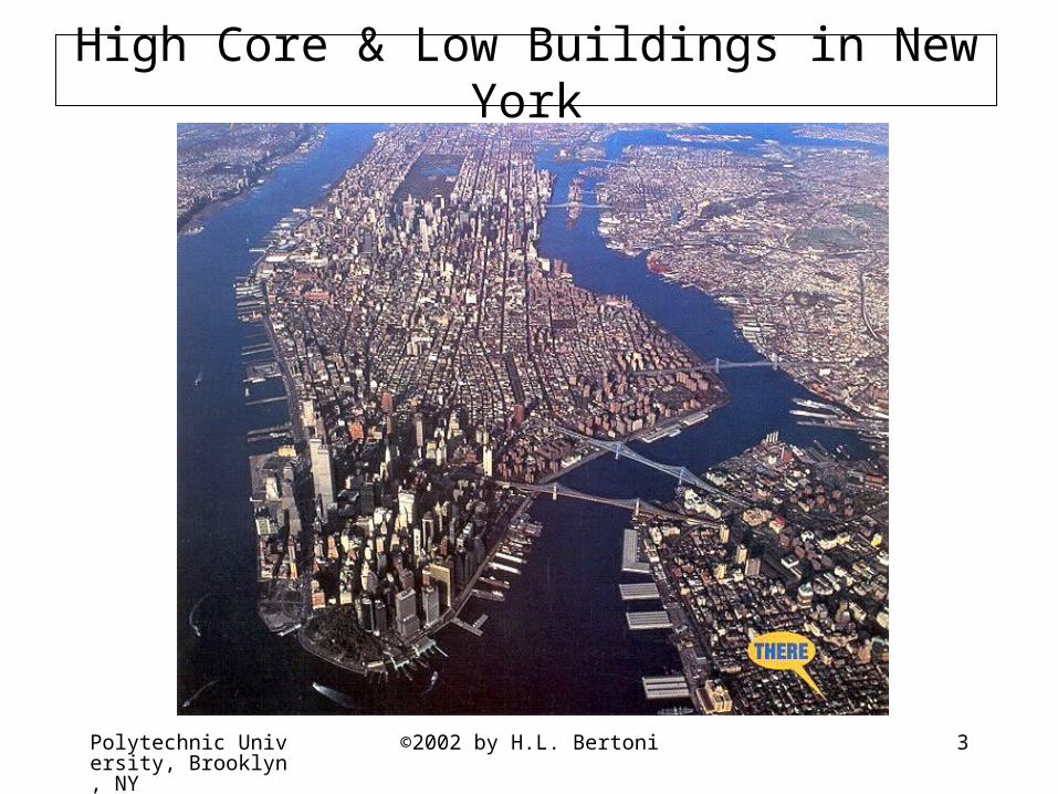
• High rise core surrounded by large areas of low buildings

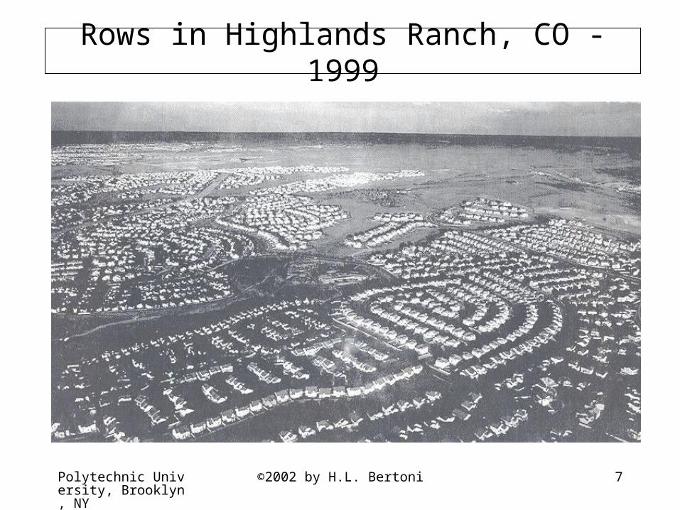
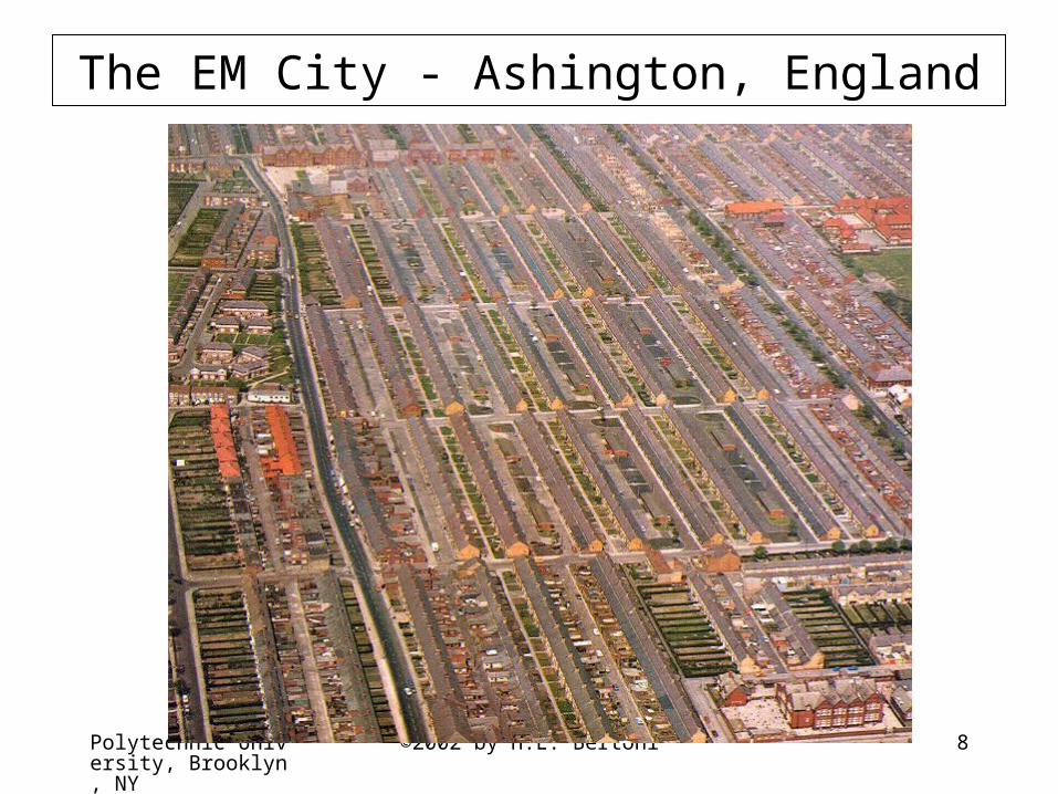
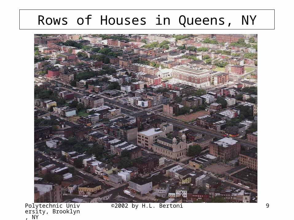
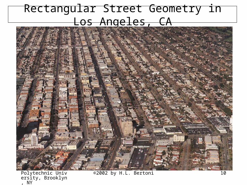
• Street grid organizes the buildings into rows



High Core & Low Buildings in New York



High Core & Low Buildings in Chicago, IL



Rows of Houses in Levittown, LI - 1951



Rows of Houses in Boca Raton, FL - 1980’s



Rows in Highlands Ranch, CO - 1999



The EM City - Ashington, England



Rows of Houses in Queens, NY



Rectangular Street Geometry in Los Angeles, CA



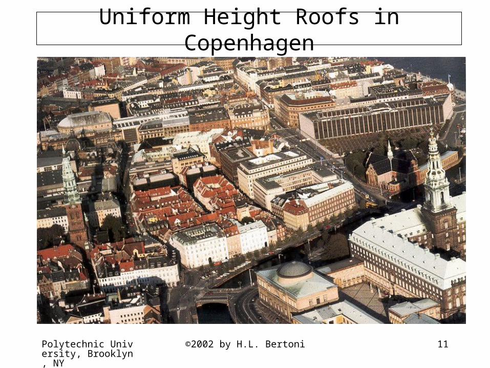
Uniform Height Roofs in Copenhagen



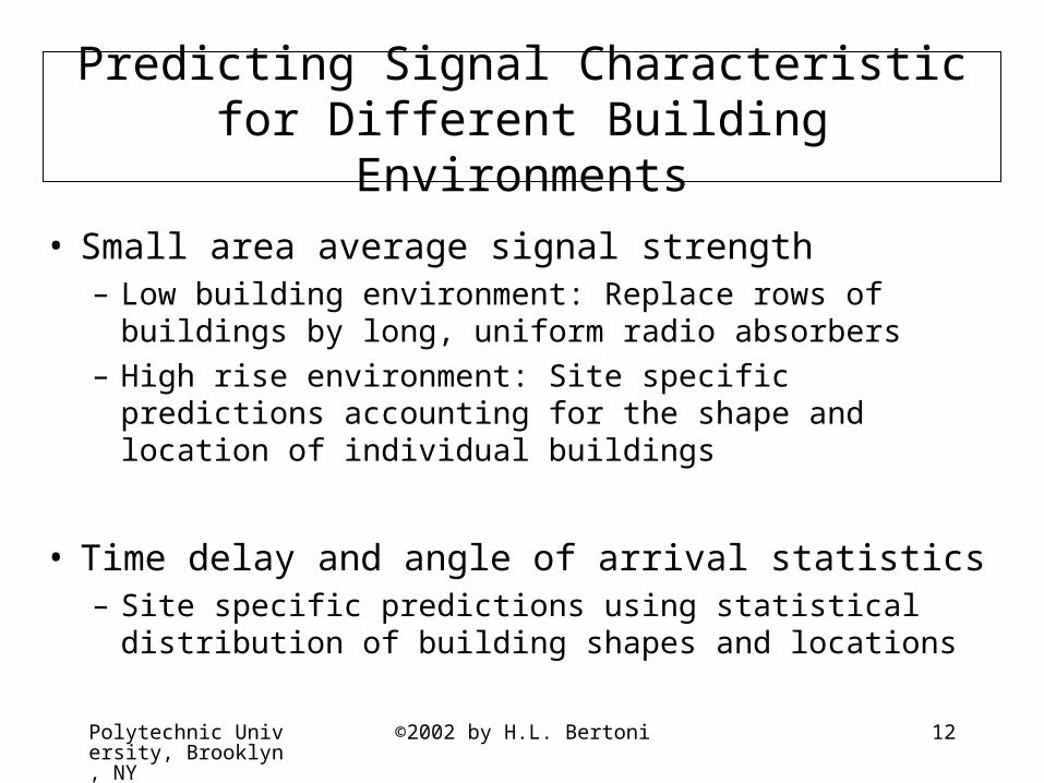
Predicting Signal Characteristic for Different Building Environments

• Small area average signal strength– Low building environment: Replace rows of buildings by

long, uniform radio absorbers

– High rise environment: Site specific predictions accounting for the shape and location of individual buildings

• Time delay and angle of arrival statistics– Site specific predictions using statistical distribution of

building shapes and locations



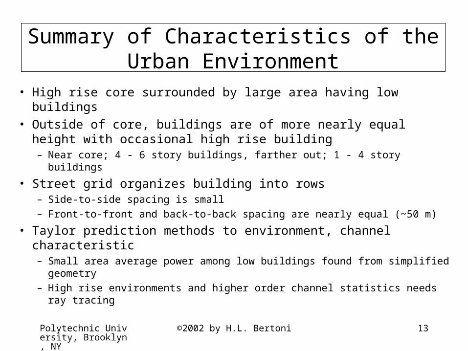
Summary of Characteristics of the Urban Environment

• High rise core surrounded by large area having low buildings

• Outside of core, buildings are of more nearly equal height with occasional high rise building– Near core; 4 - 6 story buildings, farther out; 1 - 4 story buildings

• Street grid organizes building into rows– Side-to-side spacing is small

– Front-to-front and back-to-back spacing are nearly equal (~50 m)

• Taylor prediction methods to environment, channel characteristic– Small area average power among low buildings found from simplified

geometry

– High rise environments and higher order channel statistics needs ray tracing



Propagation Past Rows of Low Buildings of Uniform Height

• Propagation takes place over rooftops

• Separation of path loss into three factors

• Free space loss to rooftops near mobile

• Reduction of the rooftop fields due to diffraction past previous rows

• Diffraction of rooftop fields down to street level

• Find the reduction in the rooftop fields using:– Incident Plane wave for high base station antennas

– Incident cylindrical wave for low base station antennas



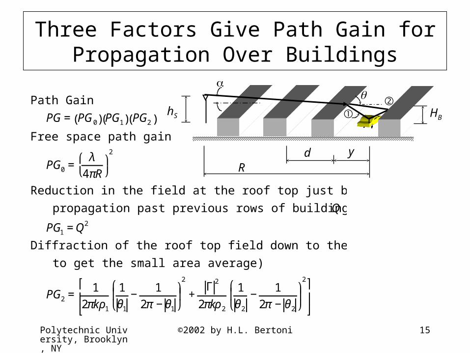
Three Factors Give Path Gain for Propagation Over Buildings

€

Path Gain

PG= PG0( ) PG1( ) PG2( )

Free space path gain

PG0 =λ

4πR⎛ ⎝

⎞ ⎠

2

Reduction in the field at the roof top just before the mobile due to

propagation past previous rows of buildings given by a factor Q

PG1 =Q2

Diffraction of the roof top field down to the mobile (add ray power

to get the small area average)

PG2 =1

2πkρ1

1θ1

−1

2π −θ1

⎛

⎝ ⎜

⎞

⎠ ⎟

2

+Γ

2

2πkρ2

1θ2

−1

2π −θ2

⎛

⎝ ⎜

⎞

⎠ ⎟

2⎡

⎣ ⎢

⎤

⎦ ⎥

dR

y

HBhS



Roof Top Fields Diffract Down to Mobile(First proposed by Ikegami)

hB

Because and 2~ 0.1,rays and have nearly equalamplitudes. Adding power isapproximately the same asdoubling the power of .

€

PG2 ≈1

πkρ1θ

−1

2π −θ

⎛

⎝ ⎜

⎞

⎠ ⎟

2⎡

⎣ ⎢

⎤

⎦ ⎥ ≈

1πkρθ2 =

λ2π 2ρθ2

where

θ =sin−1 HB −hm

ρ

⎛

⎝ ⎜ ⎞

⎠ ≈

HB −hm

ρ and ρ = HB −hm( )

2+y2

PG2 =λρ

2π2(HB −hm)2

⎡

⎣ ⎢ ⎤

⎦ ⎥



Comparison of Theory for Mobile Antenna Height Gain with Measurements

Median value of measurements made at many locations for 200MHz signalsin Reading, England, whose nearly uniform height HB=12.5 m.



Summary of Propagation Over Low Buildings

• A heuristic argument has been made for separating the path gain into three factors– Free space path gain to the building before the mobile

– Reduction Q of the roof top fields due to diffraction past previous rows of buildings

– Diffraction of the rooftop fields down to the mobile

• Diffraction of the rooftop gives the observed height gain for the mobile antenna.



Computing Q for High Base Station Antennas

• Approximating the rows of buildings by a series of diffracting screens

• Finding the reduction factor using an incident plane wave

• Settling behavior of the plane wave solution and its interpretation in terms of Fresnel zones

• Comparison with measurements



Approximations for Computing Q Effect of previous rows on the field at top of last row of building before mobile

• External and internal walls of buildings reflect and scatter incident waves - waves propagate over the tops of buildings not through the buildings.

• Gaps between buildings are usually not aligned with path from base station to mobile - replace individual buildings by connected row of of buildings.

• Variations in building height effect the shadow loss, but not the range dependence - take all buildings to be the same height.

• Forward diffraction through small angles is approximately independent of object cross section - replace rows of buildings by absorbing screens.

• For high base station antenna and distances greater than 1 km, the effect of the buildings on spherical wave field is the same as for a plane wave - Q() found for incident plane wave.

• For short ranges and low antennas, the effect of buildings on spherical wave field is the same as for a cylindrical wave - find QM for line source.



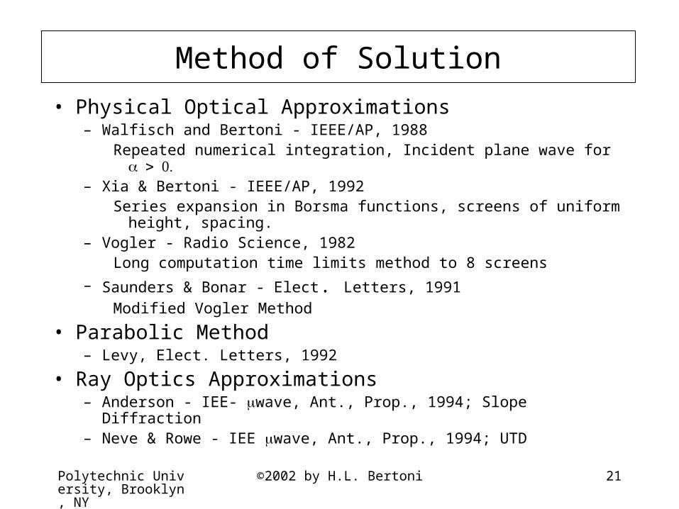
Method of Solution

• Physical Optical Approximations– Walfisch and Bertoni - IEEE/AP, 1988

Repeated numerical integration, Incident plane wave for – Xia & Bertoni - IEEE/AP, 1992

Series expansion in Borsma functions, screens of uniform height, spacing.– Vogler - Radio Science, 1982

Long computation time limits method to 8 screens

– Saunders & Bonar - Elect. Letters, 1991

Modified Vogler Method

• Parabolic Method– Levy, Elect. Letters, 1992

• Ray Optics Approximations– Anderson - IEE- wave, Ant., Prop., 1994; Slope Diffraction– Neve & Rowe - IEE wave, Ant., Prop., 1994; UTD



Plane Wave Solution for High BaseStation Antennas

–Reduction of rooftop fields for a spherical wave incident on the rows of buildings is the is the same as the

reduction for an incident plane wave after many rows.

–Reduction is found from multiple forward diffraction past an array of absorbing screens for a plane wave with unit amplitude that is incident at glancing the angle



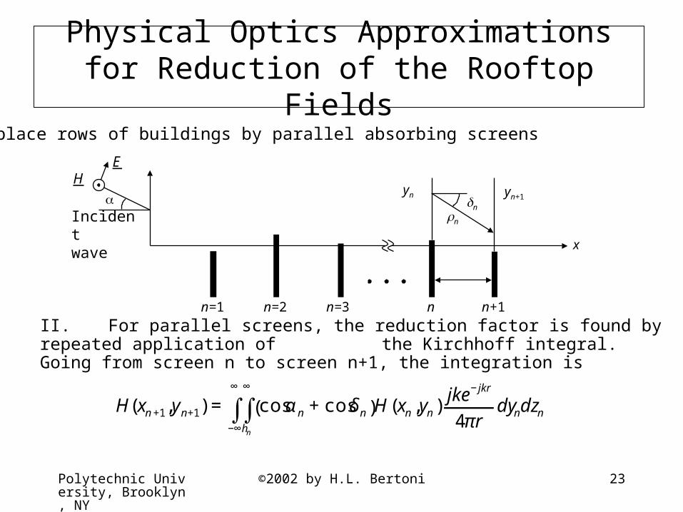
Physical Optics Approximations for Reduction of the Rooftop Fields

I. Replace rows of buildings by parallel absorbing screens

II. For parallel screens, the reduction factor is found by repeated application of the Kirchhoff integral. Going from screen n to screen n+1, the integration is

H(xn+1,yn+1) = cosαn +cosδn( )H(xn,yn)jke−jkr

4πrdyn

hn

∞

∫ dzn−∞

∞

∫

n

n

yn

x

n=1 n=2 n=3 n n+1

€

E

€

H

Incidentwave

yn+1



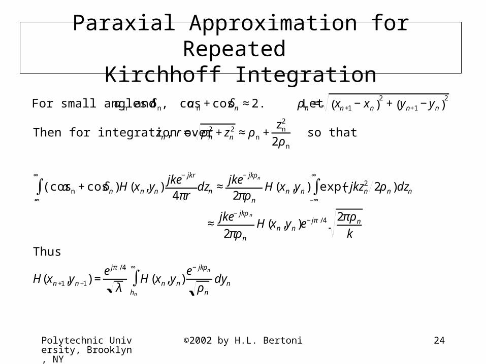
Paraxial Approximation for Repeated Kirchhoff Integration

€

For small angles αn and δn, cosαn +cosδn ≈2. Let ρn = xn+1 −xn( )2+ yn+1 −yn( )

2

Then for integration over zn, r = ρn2 +zn

2 ≈ρn +zn

2

2ρn

so that

(cosαn +cosδn)H(xn,yn)jke−jkr

4πr-∞

∞

∫ dzn ≈jke−jkρn

2πρn

H(xn,yn) exp(−jkzn2 2ρn)dzn

−∞

∞

∫

≈jke−jkρn

2πρn

H(xn,yn)e−jπ /4 2πρn

k

Thus

H(xn+1,yn+1) =ejπ /4

λH(xn,yn)

hn

∞

∫ e−jkρn

ρn

dyn



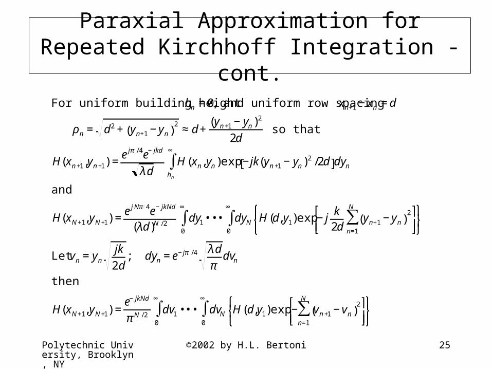
Paraxial Approximation forRepeated Kirchhoff Integration - cont.

€

For uniform building height hn =0, and uniform row spacing xn+1 −xn =d

ρn = d2 + yn+1 −yn( )2

≈d+(yn+1 −yn)

2

2d so that

H(xn+1,yn+1) =ejπ /4e−jkd

λdH(xn,yn)

hn

∞

∫ exp−jk(yn+1 −yn)2 /2d[ ]dyn

and

H(xN+1,yN+1) =ejNπ 4e−jkNd

(λd)N /2 dy10

∞

∫ ••• dyN0

∞

∫ H(d,y1)exp−jk2d

yn+1 −yn( )2

n=1

N

∑⎡

⎣ ⎢ ⎤

⎦ ⎥ ⎧ ⎨ ⎩

⎫ ⎬ ⎭

Let vn =ynjk2d

; dyn =e−jπ /4 λdπ

dvn

then

H(xN+1,yN+1) =e−jkNd

πN /2 dv10

∞

∫ ••• dvN0

∞

∫ H(d,y1)exp− vn+1 −vn( )2

n=1

N

∑⎡

⎣ ⎢ ⎤

⎦ ⎥ ⎧ ⎨ ⎩

⎫ ⎬ ⎭



Rooftop Field for Incident Plane Wave

€

H(d,y1) =e−jkdcosαe jky1sinα ≈e−jkde jky1sinα

Use Taylor series expansion

H(d,y1) =e−jkdejky1 sinα =e−jkd 1q!

( jky1sinα)q

q=0

∞

∑

Define gp =sinαdλ

and since ν1 =y1jk2d

, then

H(d,y1) =e−jkdejky1 sinα =e−jkd 1q!

2gp jπ( )qν1

q

q=0

∞

∑

Then the field at yN+1 =0 νN+1 =0( ) is

H(xN+1,0)=e−jk(N+1)d

π N /2 dν1 •••0

∞

∫ dνN0

∞

∫ 1q!

2gp jπ( )qν1

q

q=0

∞

∑⎡

⎣ ⎢ ⎤

⎦ ⎥ exp−ν12 +2 νn+1νn −2 νn

2

n=2

N

∑n=1

N−1

∑⎡

⎣ ⎢ ⎤

⎦ ⎥ ⎧ ⎨ ⎩

⎫ ⎬ ⎭

H(xN+1,0)=e−jk(N+1)d 1q!

2gp jπ( )qIN ,q(1)

q=0

∞

∑ ,

where IN,q(1) is a Borsma function defined in the next slide.



€

IN,q 1( ) =1

πN /2 dν1 dν20

∞

∫0

∞

∫ ••• dνN0

∞

∫ ν1q exp−ν1

2 +2 νn+1νnn=1

N−1

∑ −2 νn2

n=2

N

∑⎡

⎣ ⎢ ⎤

⎦ ⎥ ⎧ ⎨ ⎩

⎫ ⎬ ⎭

Recursion relation for q≥2

IN,q β( )=N(q−1)

2(N +1)β−1 IN ,q−2 β( )+1

2 π (N +1)β−1

I n,q−1 β( )

N −nn=β−1

N−1

∑

where

I0,q(1) =1 for q=0

0 for q>0⎧ ⎨ ⎩

IN,0(1)=(1/2)N

N!; IN,1(1)=

1

2 π

(1/2)n

n! N −nn=0

N−1

∑The term (1/2)n represents Pockhammer's Symbol for a=1/2, where

(a)0 =1; (a)1 =a; (a)n =a(a+1)L (a+n−1)

Borsma Functions for = 1



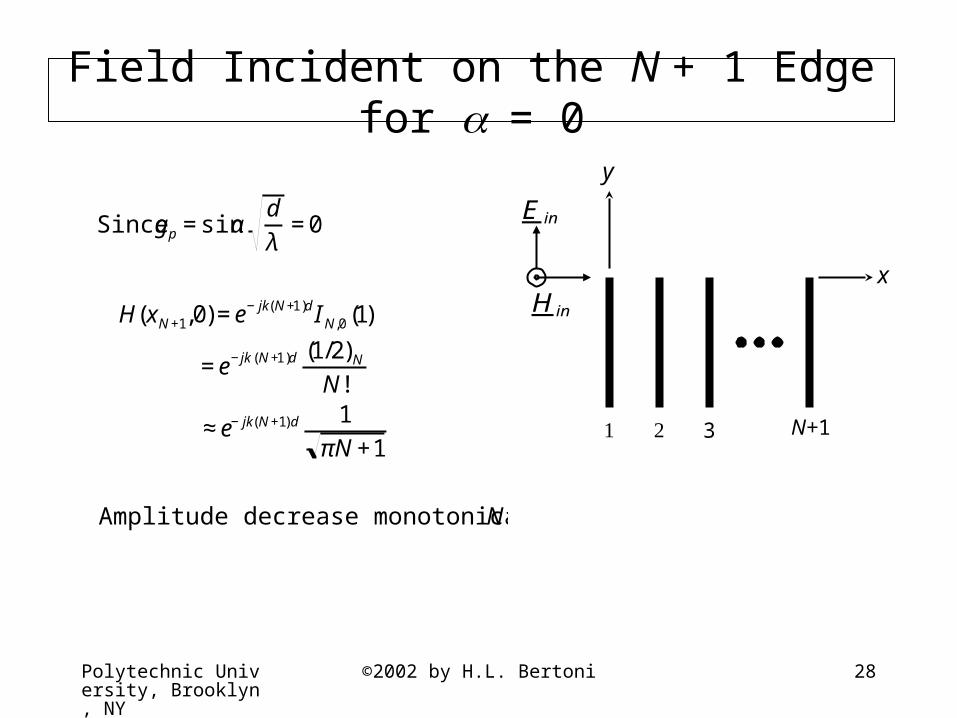
Field Incident on the N + 1 Edge for = 0

3 N+1

€

E in

€

H in

x

y

€

Since gp =sinαdλ

=0

H(xN+1,0)=e−jk(N+1)dIN,0(1)

=e−jk(N+1)d (1/2)N

N!

≈e−jk(N+1)d 1πN +1

Amplitude decrease monotonically with N



Field Incident on the N + 1 Edge for ≠ 0

After initial variation, field settles to a constant value Q(gp) for N > N0

20 1;sin pp gN

dg ==

λ

N0

SettledFieldQ(gp)

Angles indicatedare ford =200λ

1 2 …. n n+1

…



Explanation of the Settling Behavior in Terms of the Fresnel Zone About the Ray Reaching the N+1 Edge

Only those edges that penetrate the Fresnel zone affect the field at the N +1 edge

N0 =λ / d

sin2α=

1gp

2

d

n=1 n=3 n=5 n=N n=N +1

€

E1

n=2 n=4

€

H1

N0

n=N -1

λ secNd

tanNdN0dtanα = N0dλ secα

€

Fresnel zone half width

WF = λs



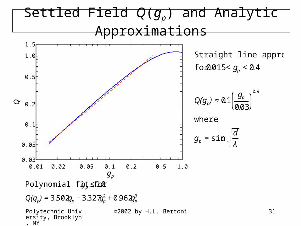
Settled Field Q(gp) and Analytic Approximations

0.01 0.02 0.05 0.1 0.2 0.5 1.00.03

0.05

0.1

0.2

0.5

1.0

1.5

Q

gp

Straight line approximation

for 0.015<gp <0.4

Q(gp) ≈0.1gp

0.03

⎛ ⎝ ⎜ ⎞

⎠

0.9

where

gp =sinαdλ

Polynomial fit for gp ≤1.0

Q(gp) =3.502gp −3.327gp2 +0.962gp

3



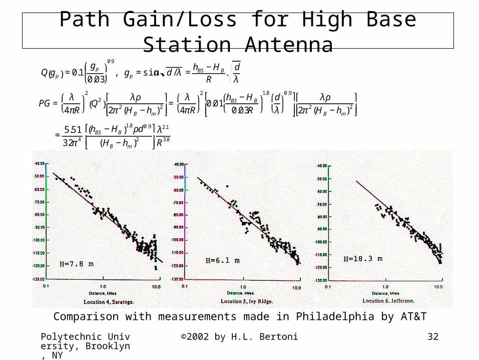
Path Gain/Loss for High Base Station Antenna

Comparison with measurements made in Philadelphia by AT&T

€

Q gp( ) ≈0.1gp

0.03

⎛

⎝ ⎜ ⎞

⎠

0.9

, gp =sinα d/λ ≈hBS −HB

Rdλ

PG=λ

4πR⎛ ⎝

⎞ ⎠

2

Q2( )

λρ2π2(HB −hm)2

⎡

⎣ ⎢ ⎤

⎦ ⎥ =λ

4πR⎛ ⎝

⎞ ⎠

2

0.01hBS −HB

0.03R⎛ ⎝

⎞ ⎠

1.8dλ

⎛ ⎝

⎞ ⎠

0.9⎡

⎣ ⎢ ⎤

⎦ ⎥ λρ

2π2(HB −hm)2

⎡

⎣ ⎢ ⎤

⎦ ⎥

=5.5132π4

hBS −HB( )1.8ρd0.9

(HB −hm)2

⎡

⎣ ⎢

⎤

⎦ ⎥

λ2.1

R3.8



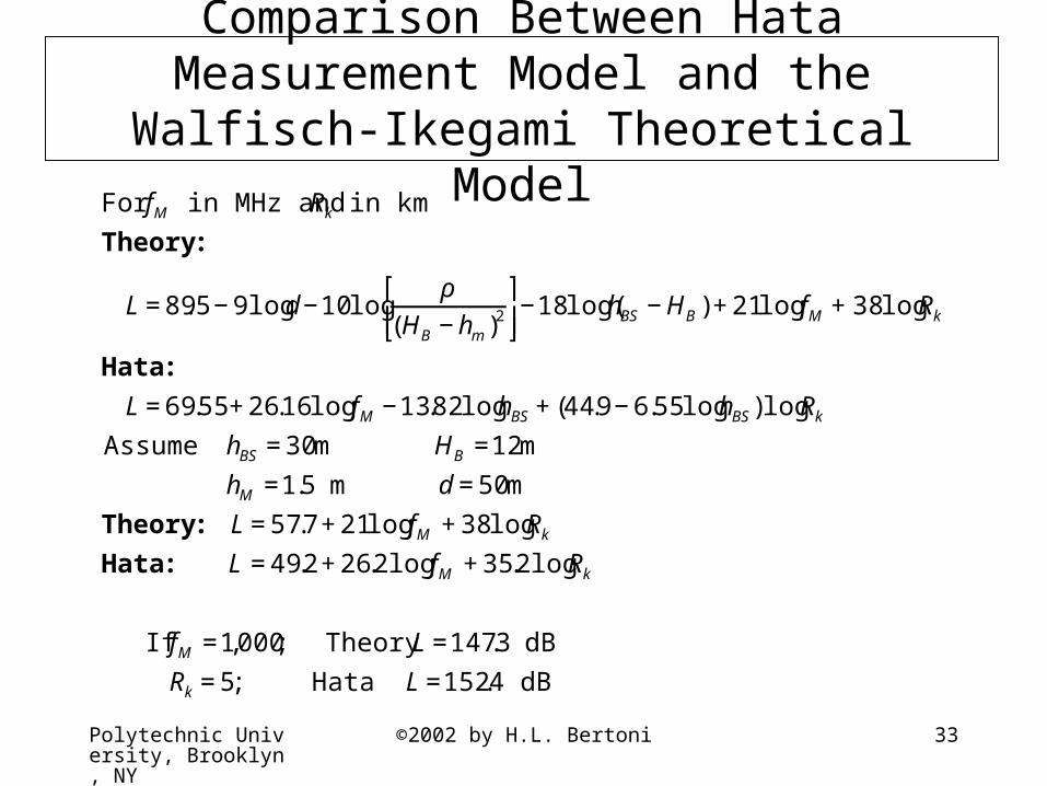
Comparison Between Hata Measurement Model and the Walfisch-Ikegami Theoretical Model

€

For fM in MHz and Rk in km

Theory:

L =89.5−9logd−10logρ

(HB −hm)2

⎡

⎣ ⎢ ⎤

⎦ ⎥ −18log(hBS −HB)+21logfM +38logRk

Hata:

L =69.55+26.16logfM −13.82loghBS +(44.9−6.55loghBS)logRk

Assume hBS =30m HB =12m

hM =1.5 m d=50m

Theory: L =57.7+21logfM +38logRk

Hata: L =49.2+26.2logfM +35.2logRk

If fM =1,000; Theory L =147.3 dB

Rk =5; Hata L =152.4 dB



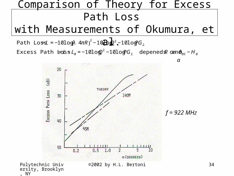
Comparison of Theory for Excess Path Loss with Measurements of Okumura, et al.

€

Path Loss =L =−10logλ 4πR( )2−10logQ2 −10logPG2

Excess Path Loss =L −L0 =−10logQ2 −10logPG2 depeneds on R and hBS −HB

only through the angle α

f = 922 MHz



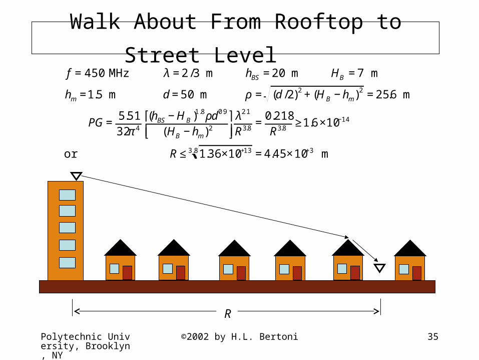
Walk About From Rooftop to Street Level

€

f =450 MHz λ =2/3 m hBS =20 m HB =7 m

hm =1.5 m d=50 m ρ = (d/2)2 +(HB −hm)2 =25.6 m

PG=5.5132π4

(hBS −HB)1.8ρd0.9

(HB −hm)2

⎡

⎣ ⎢ ⎤

⎦ ⎥ λ2.1

R3.8 =0.218R3.8 ≥1.6×10−14

or R≤ 1.36×10+133.8 =4.45×10+3 m

R



Summary of Q for High Base Station Antennas

• Rows of buildings act as a series of diffracting screens

• Forward diffraction reduces the rooftop field by a factor that approaches a constant past many rows

• The settling behavior can be understood in terms of Fresnel zones, and leads to the reduction factor Q, which depends on a single parameter gp

• Good comparison with measurements is obtained using a simple power expansion for Q



Cylindrical Wave Solution for Low Base Station Antennas

• Finding the reduction factor Q using an incident cylindrical wave

• Q is shown to depend on parameter gc and the number of rows of buildings

• Comparison with measurements• Mobile-to-mobile communications



Cylindrical Wave Solutions for Microcells Using Low Base Station Antennas

Microcell coverage out to about 1 km involves propagation over a limited number of rows.

Must account for the number of rows covered, and hence for the field variation in the plane perpendicular to the rows of buildings.

Therefore use a cylindrical incident wave with axis parallel to the array of absorbing screens to find the field reduction due to propagation past rows of buildings.



Physical Optics Approximations for Reductionof the Rooftop Fields

I. Replace rows of buildings by parallel absorbing screens

II. For parallel screens, the reduction factor will apply for a spherical wave and for a cylindrical wave. For 2D fields, Kirchhoff integration gives

H(xn+1,yn+1) = cosαn +cosδn( )H(xn,yn)jke−jkr

4πrdyn

hn

∞

∫ dzn−∞

∞

∫

≈ejπ / 4

λH(xn,yn)

e−jkρn

ρn

dynhn

∞

∫ , since cosαn +cosδn ≈2

n

n

yn

x

n=1 n=2 n=3 n n+1

€

E

€

H

Incidentwave

yn+1



Paraxial Approximation for Repeated Kirchhoff Integration and Screens of Uniform Height

€

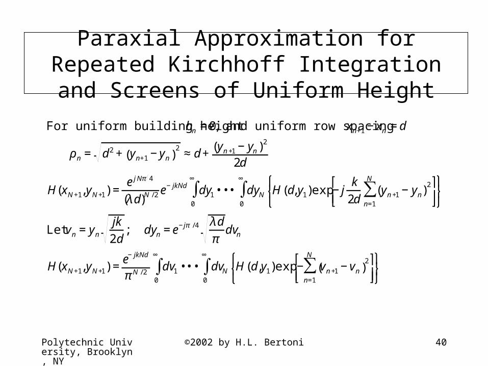
For uniform building height hn =0, and uniform row spacing xn+1 −xn =d

ρn = d2 + yn+1 −yn( )2

≈d+(yn+1 −yn)

2

2d

H(xN+1,yN+1) =ejNπ 4

(λd)N /2 e−jkNd dy10

∞

∫ ••• dyN0

∞

∫ H(d,y1)exp−jk

2dyn+1 −yn( )

2

n=1

N

∑⎡

⎣ ⎢ ⎤

⎦ ⎥ ⎧ ⎨ ⎩

⎫ ⎬ ⎭

Let vn =yn

jk2d

; dyn =e−jπ /4 λdπ

dvn

H(xN+1,yN+1) =e−jkNd

πN /2 dv10

∞

∫ ••• dvN0

∞

∫ H(d,y1)exp− vn+1 −vn( )2

n=1

N

∑⎡

⎣ ⎢ ⎤

⎦ ⎥ ⎧ ⎨ ⎩

⎫ ⎬ ⎭



Approximation for Cylindrical Wave of a Line Source

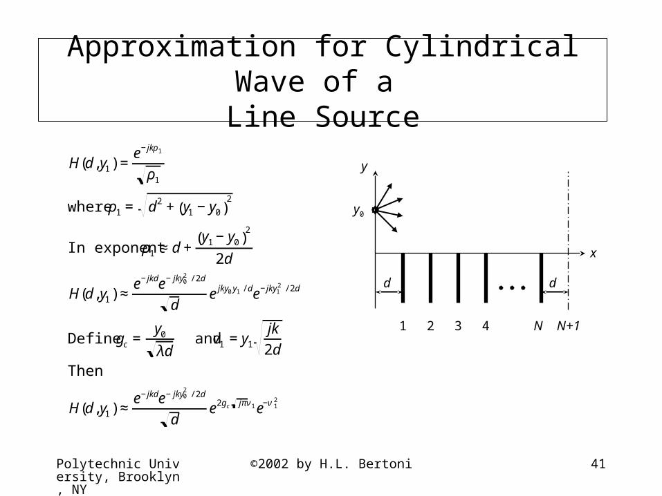
H(d,y1) =e−jkρ1

ρ1

where ρ1 = d2 + y1 −y0( )2

In exponent ρ1 ≈d+y1 −y0( )

2

2d

H(d,y1) ≈e−jkde−jky0

2 / 2d

dejky0y1 / de−jky1

2 / 2d

Define gc =y0

λd andv1 =y1

jk2d

Then

H(d,y1) ≈e−jkde−jky0

2 / 2d

de2gc jπν1e−ν 1

2

1

y

x

y0

d

2 3 4 N N+1

d



Integral Representation for Field at the N+1 Edge

€

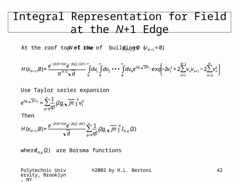
At the roof top of the N +1 row of buildings yN+1 =0 νN+1 =0( )

H(xN+1,0)=e−jk N+1( )de−jky0

2 (2d)

π N /2 ddv1 dv2

0

∞

∫0

∞

∫ ••• dvN0

∞

∫ e2gc jπν 1 exp−2v12 +2 vnvn+1

n=1

N−1

∑ −2 vn2

n=2

N

∑⎛

⎝ ⎜ ⎞

⎠ ⎟

Use Taylor series expansion

e2gc jπ v1 =1q!

2gc jπ( )qv1

q

q=0

∞

∑

Then

H(xN+1,0)=e−jk N+1( )de−jky0

2 (2d)

d1q!

2gc jπ( )qIN ,q(2)

q=0

∞

∑

where IN,q(2) are Borsma functions



€

IN,q 2( ) =1

πN /2 dν1 dν20

∞

∫0

∞

∫ ••• dνN0

∞

∫ ν1q exp−2ν1

2 +2 νn+1νnn=1

N−1

∑ −2 νn2

n=2

N

∑⎡

⎣ ⎢ ⎤

⎦ ⎥ ⎧ ⎨ ⎩

⎫ ⎬ ⎭

Recursion relation for q≥2

IN,q β( )=N(q−1)

2(N +1)β−1 IN ,q−2 β( )+1

2 π (N +1)β−1

I n,q−1 β( )

N −nn=β−1

N−1

∑

where

IN,0(2)=1

N +1( )32; IN,1(2) =

14 π

1

n23 N +1−n( )

32n=1

N

∑

Borsma Functions for Line Source Field



Rooftop Field Reduction Factor for Low Base Station Antenna

€

Reduction factor found from cylindrical wave field

QN+1(gc) =H(xN+1,0)

e−jkρ / ρ where ρ= (N +1)d[ ]

2 +y02 ≈(N +1)d

In terms of Boersma functions

QN+1(gc) = N +11q!

2gc jπ( )q=0

∞

∑q

IN ,q(2)

For y0 =0, gc =y0

λd=0 and

QN+1(gc) = N +11

(N +1)3/2 =1

N +1



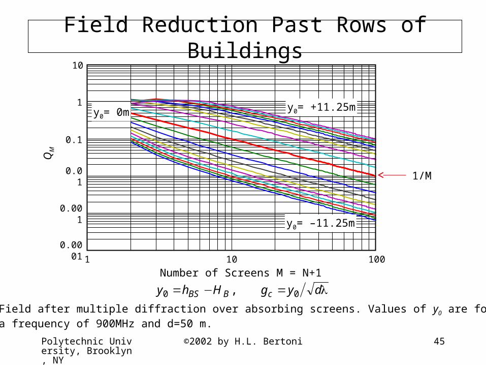
Field Reduction Past Rows of Buildings

Field after multiple diffraction over absorbing screens. Values of y0 are for a frequency of 900MHz and d=50 m.

λ=−= dygHhy cBBS 00 ,

Number of Screens M = N+11 10 100

10

1

0.1

0.01

0.001

0.0001

QM

y0= +11.25m

y0= –11.25m

y0= 0m

1/M



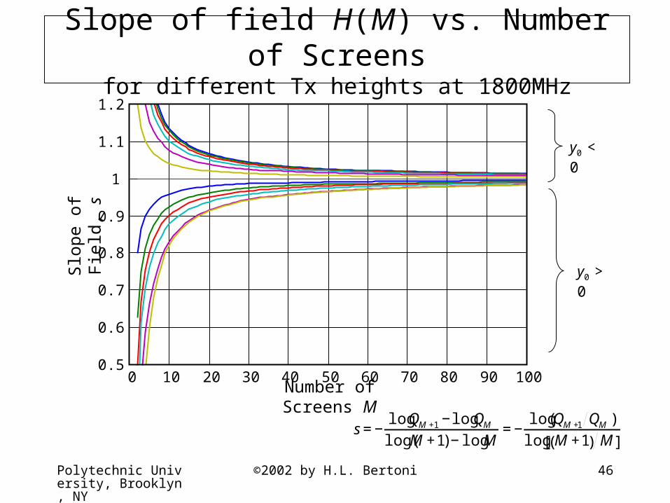
Slope of field H(M) vs. Number of Screensfor different Tx heights at 1800MHz

0 10 20 30 40 50 60 70 80 90 1000.5

0.6

0.7

0.8

0.9

1

1.1

1.2

Number of Screens M

Slop

e of

Fie

ld, s

y0 < 0

y0 > 0



Modifications for Propagation Oblique to the Street Grid

Base Station

x

R

x=0

mobile

Radio propagation with oblique incidencex = Md + d/2

€

PG2 =10log1

πkr⊥cosφ1

θ⊥

−1

2π +θ⊥

⎛

⎝ ⎜ ⎞

⎠ ⎟

2⎡

⎣ ⎢

⎤

⎦ ⎥ gc =y0

cosφλd



Comparison of Base Station Height Gain with Har/Xia Measurement Model

€

f =1.8 GHz

d=50 m

y0 =hBS −HB

R=1 km

For perpendicular propagation

φ =0

N +1=Rd

=20

For oblique propagation

φ =60°

N +1=R

d/cosφ=10-8 -6 -4 -2 0 2 4 6 8

-50

-45

-40

-35

-30

-25

-20

-15

-10

-5

0

Q in

dB

y0

Q10

Q20

Qexp



Experimentally Based Expression for Qexp

€

We can compare the theoretical Q with the Har/Xia measurements using

L =−PG =−PG0 −20logQ−PG2

The Har/Xia formulas for path loss on staircase and transverse paths give

L, so that

20logQexp=−L −PG0 −PG2

Substituing their expression for L gives

20logQexp=− 138.3+38.9logfG[ ]{

−13.7−4.6logfG[ ]sgn(y0)log1+ y0( )

+40.1−4.4sgn(y0)log1+y0( )[ ]logRk}

−10logλ

4πRk ×103

⎛

⎝ ⎜ ⎞

⎠ ⎟

2

−10logλρ

2π 2(HB −hm)2

⎡

⎣ ⎢ ⎤

⎦ ⎥



Comparison of Range Index n with Har/Xia Measurement Model

km

m

GHz

2/1

50

8.1

Rdf

n=2+2s

-8 -6 -4 -2 0 2 4 6 83.4

3.5

3.6

3.7

3.8

3.9

4

4.1

4.2

4.3

4.4

n

y0

theoryexp



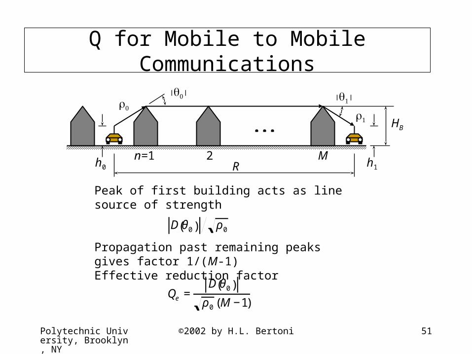
Q for Mobile to Mobile Communications

h0 h1Rn=1 2 M

HB

Peak of first building acts as line source of strength

Propagation past remaining peaks gives factor 1/(M-1)Effective reduction factor

Dθ0( ) ρ0

Qe =Dθ0( )

ρ0 (M −1)



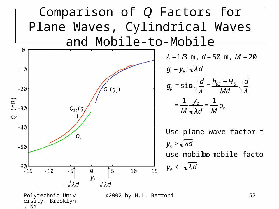
Comparison of Q Factors for Plane Waves, Cylindrical Waves and Mobile-to-Mobile

€

λ =1/3 m, d=50 m, M =20

gc =y0 λd

gp =sinαdλ

=hBS −HB

Mddλ

=1M

y0

λd=

1M

gc

Use plane wave factor for

y0 > λd

use mobile- to-mobile factor for

y0 <− λd-15 -10 -5 0 5 10 15

-60

-50

-40

-30

-20

-10

0

Q (

dB)

y0

Q20(gc)

Q (gp)

Qe

dλ− dλ



Path Loss for Mobile-to-Mobile Communication

L =−20logλ

4πR⎛ ⎝

⎞ ⎠

−20logQe −10logD1

2

ρ1

Since R=Md

L =−20logλ4π

⎛ ⎝

⎞ ⎠

+20logdM(M −1)[ ]−10logD0

2

ρ0

−10logD1

2

ρ1

If both mobile are at same height and in the middle of the street, using

D 2

ρ≈

12πkρ

1θ 2 ≈

12πk(d /2)

d /2HB −hm

⎛

⎝ ⎜ ⎞

⎠ ⎟

2

=dλ

8π2(HB −hm)2

gives

L =20log(16π3)+20logM(M −1)[ ]+40logHB −hm

λ⎛ ⎝

⎞ ⎠



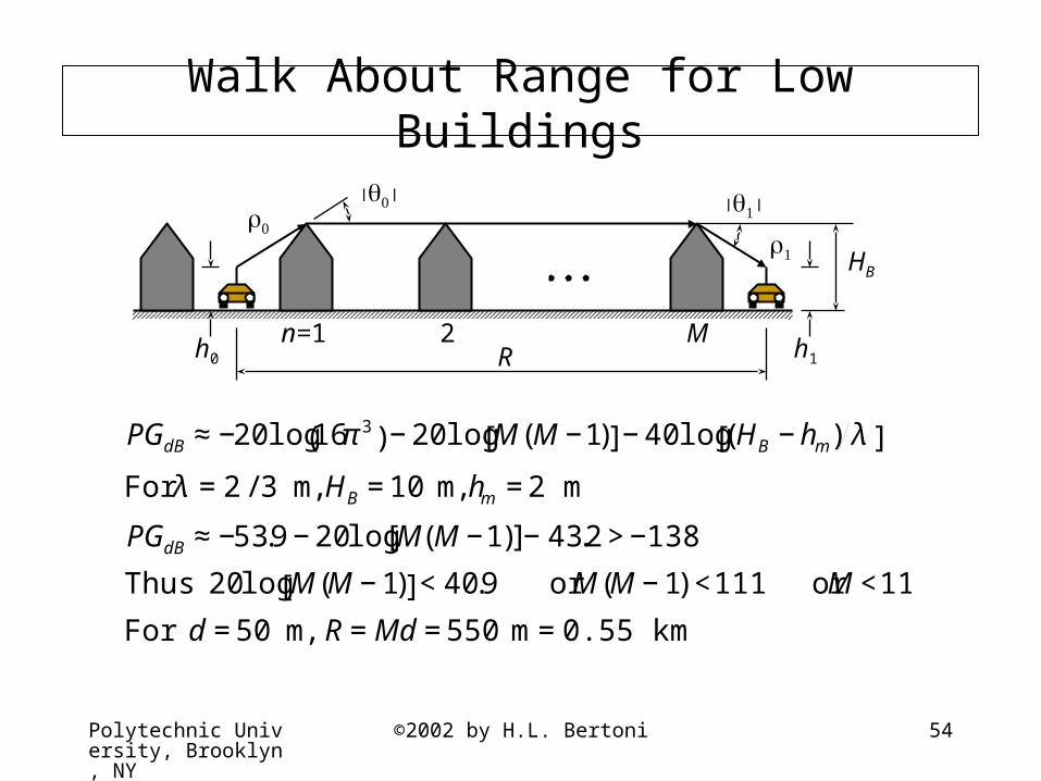
h0 h1Rn=1 2 M

HB

PGdB ≈−20log16π3( )−20logM(M −1)[ ]−40log(HB −hm) λ[ ]

For λ =2/ 3 m, HB =10 m, hm =2 m

PGdB ≈−53.9−20logM(M −1)[ ]−43.2>−138

Thus 20logM(M −1)[ ]<40.9 or M(M −1) <111 or M <11

For d =50 m, R=Md =550 m =0.55 km

Walk About Range for Low Buildings



Summary of Solution for Low BaseStation Antennas

• Reduction factor found using an incident cylindrical wave

• QM depends on parameter gc and the number of rows of buildings M over which the signal passes

• Theory gives the correct trends for base station height gain and slope index, but is pessimistic for antennas below the rooftops

• Theory give simple expressions for path gain in the case of Mobile-to-mobile communications

Polytechnic University, Brooklyn, NY ©2002 by H.L. Bertoni1 IX. Modeling Propagation in Residential Areas Characteristics of City Construction Propagation.

Documents

polytechnic university

ny slide

rows of buildings

ca slide

copenhagen slide

il slide

s slide

england slide