Polynomial trajectory algorithm for a biped robot

International Journal of Robotics and Automation, Vol. 25, No. 4, 2010

POLYNOMIAL TRAJECTORY ALGORITHM

FOR A BIPED ROBOT

Erik Cuevas,∗,∗∗Daniel Zaldivar,∗,∗∗Marco Perez-Cisneros,∗ and Marte Ramırez-Ortegon∗∗

Abstract

Building trajectories for biped robot walking is a complex task

considering all degrees of freedom (DOFs) commonly bound within

the mechanical structure. A typical problem for such robots is the

instability produced by violent transitions between walking phases

in particular when a swinging leg impacts the surface. Although

extensive research on novel efficient walking algorithms has been

conducted, falls commonly appear as the walking speed increases or

as the terrain condition changes. This paper presents a polynomial

trajectory generation algorithm (PTA) to implement the walking on

biped robots following the cubic Hermitian polynomial interpolation

between initial and final conditions. The proposed algorithm allows

smooth transitions between walking phases, significantly reducing

the possibility of falling. The algorithm has been successfully tested

by generating walking trajectories under different terrain conditions

on a biped robot of 10 DOFs. PTA has shown to be simple and

suitable to generate real-time walking trajectories, despite reduced

computing resources of a commercial embedded microcontroller.

Experimental evidence and comparisons to other state-of-the-art

methods demonstrates a better performance of the proposed method

in generating walking trajectories under different ground conditions.

Key Words

Biped robots, trajectory generation, dynamic walking

1. Introduction

Robots must successfully deal with complicated environ-ments such as rugged terrain, sloped surfaces, and steepstairs. Although it is assumed that biped robots canwalk in almost any type of terrain surpassing some of thewheeled robots capabilities [1–3], they are complex non-linear systems with many degrees of freedom (DOFs) thatmay fall down easily while walking due to its relativelysmall feet and other important design constraints.

A popular technique to implement biped walking is tokeep the zero moment point (ZMP) constraint within a

∗ CUCEI, Departamento de Electronica, Universidad deGuadalajara, Av. Revolucion 1500, C.P. 44430 Guadala-jara, Jal., Mexico; e-mail: {daniel.zaldivar, erik.cuevas, marco.perez}@cucei.udg.mx

∗∗ Institut fur Informatik, Freie Universitat Berlin, Takustr. 9,14195 Berlin, Germany; e-mail: [email protected]

Recommended by Dr. A.M. Khamis(10.2316/Journal.206.2010.4.206-3240)

supporting feet polygon to ensure stable walking gaits [4].Several methods have been proposed to generate walkingtrajectories satisfying this condition such as those referredin [5–17]. They fall into two groups: time-dependentand time-invariant algorithms. By far, the most popularalgorithms are time-dependent which involve the trackingof pre-calculated trajectories. The second group requiresthe precise knowledge of biped dynamics to solve complexnonlinear models to generate walking patterns. This paperfocuses only on the time-dependent algorithms.

Several techniques for generating walking motion forbiped robots may be found in the literature. For instance,Ohishi et al. [11] approximated the biped movement asa three-dimensional inverted pendulum model (IPM), us-ing the resulting points as tracking reference in Cartesianspace. Some other algorithms with small variations of IPMcan also be found. In [17] the IPM is transformed into acart-table model, with the cart movements correspondingto the trajectory of the centre of mass (CoM). In [12] and[13], Kajita et al. demonstrated the use of a length-varyinginverted pendulum as reference point to generate trajecto-ries. The pendulum’s length varies as to keep the biped’sCoM at a constant height above the walking surface (seealso [8]). Grishin et al. [14] used a pre-computed trajectorywith online adjustment to improve stability of the bipedrobot. Other works such as those in [5–7, 10], use a differ-ent IPM to generate the walking trajectory. Most of theworks on three-dimensional walking movements computedecoupled trajectories from the frontal and sagittal planes.Katoh and Mori [15] demonstrated that using a Van derPol oscillator as generator of the tracking reference wouldinduce walking trajectories for a biped robot. Moreover,Furusho and Masubuchi [16] presented the walking controlalgorithms by tracking a piecewise-linear joint referencetrajectory. Another method for trajectory generation isto mimic the human rhythmic function by means of acentral pattern generator, just as it is reported in [9]. Inthis method, one self-oscillating system is designed as togenerate synchronized periodic motions for each joint.Although extensive research on novel efficient walking al-gorithms has been conducted, the reported results stillshow a trend for falling down as walking speed increasesor when terrain conditions change. Slow down the walkingpace will be a temporary solution as the problem remainsunsolved as walking deterioration is inflicted on subsequent

294

walking phases. Some previous works [18] have shown thenegative effect of a violent impact between the feet and theground which yields a reaction force FR and increasesthe possibility of falls. The effect can be even worse, whenthe robots’ velocity is increased or the terrain conditionschange. Although some IPM algorithms have attemptedto solve the problem, they require extensive computationunsuitable for real-time applications.

This paper presents the polynomial trajectory algo-rithm (PTA) which is a simple and effective walking tra-jectory algorithm based on cubic Hermitian polynomialinterpolation of the kinematics positions of the robot. AHermite spline (HS) is a cubic polynomial interpolation insegments with adjustable derivatives at each control pointthat allows decreasing link’s velocities when they do reachthe target point. Therefore, the impact on the leg causedby the ground contact or by violent transitions among dif-ferent walking phases may also be reduced. The walkingtrajectory is generated for each joint, adjusting some inter-mediate positions to assure the best ZMP trajectory. Theresulting approach generates suitable bipedal walking gaitsin real time considering only modest computing resources,such as a microcontroller embedded platform. Experi-mental evidence shows the effectiveness of the method togenerate walking trajectories under different ground condi-tions. The proposed algorithm was successfully tested ona biped robot of 10 DOFs [19] under different walking con-ditions. This paper presents a comparison between severalstate-of-the-art methods and it demonstrates a better rela-tionship between the link velocities and the reaction forcesproduced by the proposed method. It reduces the ZMPinstability created by violent transitions between walkingphases such as the swinging leg impacting the surface.

This paper is organized as follows: Section 2 introducesthe biped robot model and the walking gait. Section 3 dis-cusses on the impact model and its velocity discontinuity.Section 4 describes PTA and its parameters while Section5 features the walking motions generated by the PTA,despite terrain changes. This section also discusses oncomparing the PTA performance to other related methods.Finally, Section 6 draws some conclusions.

2. Robot Model and Bipedal Walking

2.1 Robot Description

The dynamics of a biped robot is closely related to itsstructure [20]. This work employs the “Dany Walker”robot [19], built on 10 low-density aluminium links. Eachlink consists of a structure which has been carefully de-signed to allow an effective torque transmission and low de-formation. All links are connected within the biped robotstructure of 10 DOFs as shown in Fig. 1. The motors allowmovements within the frontal and sagittal plane. Figure1(a) shows the frontal plane of the robot while the Fig.1(b) shows the sagittal plane. The embedded control com-puter system is based on a PIC18F4550 microcontrollerexecuting concurrent tasks such as trajectory generation,servo-motor control, and sensor signal collection. TheZMP is estimated through data integration from pressure

Figure 1. Dany Walker robot (a) frontal plane and (b)sagittal plane.

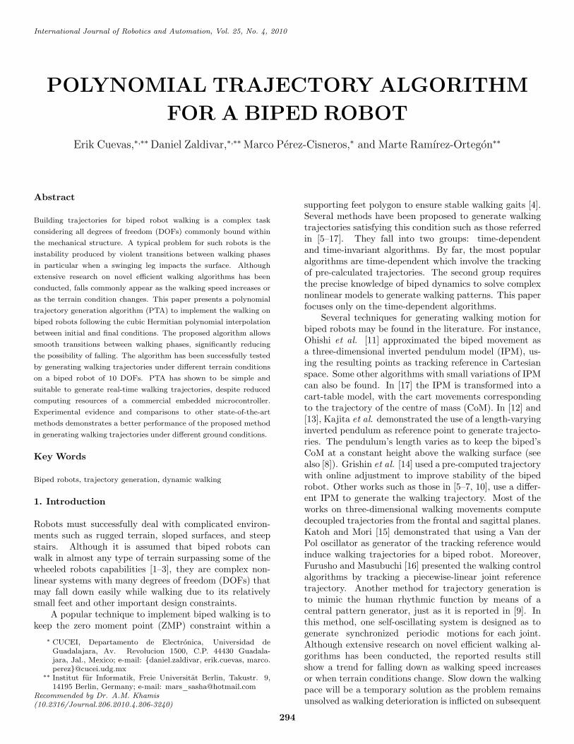
sensors (Flexiforce type) located on each foot. The centreof pressure (CoP) matches the ZMP if and only if thelatter falls inside the supporting foot polygon (SfP). In the“Dany Walker” biped robot, the ZMP was found by usingfeedback from triangular force sensor arrangement as it isdescribed in [19, 21]. Each mass is assumed to be locatedon the midpoint of its corresponding link. The parametersof the robot model according to the convention presentedin [22] are summarized in Table 1 following locations drawnin Fig. 2.

The foot’s length and width are 10 cm and 8 cm,respectively. Let position(xs, ys, zs) be middle pointof the supporting foot. Thus, the robot motion maybe expressed with respect to the reference frame whosecentre is (xs, ys, zs). The x-directional ZMP (xZMP )and the y-directional ZMP (yZMP ) should be locatedinside the region defined on −5 cm<xZMP < 5 cm and−4 cm<yZMP < 4 cm.

For the single support phase, such region is a convexhull for all contact points between the foot and the ground[10, 23]. Thus, if the ZMP falls within this area, the bipedrobot can walk without falling down [24]. However, it isdifficult to calculate the ZMP from a 3D robot model asin Fig. 1 because of the coupling motion between thefrontal plane (y–z plane) and sagittal plane (x–z plane).Therefore, the walking motion may be generated fromtwo 2D models including the sagittal plane model with8 segments and 7 DOFs as shown in Fig. 2(b). Thefrontal plane model has 6 segments and 5 DOFs as shownby Fig. 2(c). The ZMP equations of the sagittal planerobot model (Fig. 2(b)) and the frontal plane robot model(Fig. 2(c)) are:

xZMP =

7∑i=1

mi(zi + g)xi −7∑

i=1mixizi

7∑i=1

mi(zi + g)

×

yZMP =

7∑i=1

mi(zi + g)yi −7∑

i=1miyizi

7∑i=1

mi(zi + g)

(1)

with g being the gravity, (xi, yi, zi) and mi being theposition and mass of the i-th point mass (i=1, . . . , 7) [7].In (1), the inertia factors can be ignored assuming that

295

Table 1Parameters of the Biped Robot

m1 m2 m3 m4 m5 m6 m7 l1 l2 l3

0.2Kg 0.3Kg 0.3Kg 0.455Kg 0.3Kg 0.3Kg 0.2Kg 10 cm 11 cm 11 cm

l4 l5 l6 l7 lw lfl lfw lf1 lf2

10 cm 11 cm 11 cm 10 cm 11.2 cm 10 cm 8 cm 5 cm 4 cm

Figure 2. (a) Foot parameters, (b) sagittal plane, and (c) frontal plane configuration.

the mass of link i is uniformly distributed about the CoM[11, 25].

3. Impact Model and Velocity Discontinuity

This section describes the effects in terminal veloci-ties in the foot–ground impact. This condition occurswhen the swing leg touches the walking surface. LetQsbe the N -dimensional configuration space of the robotwhen the stance leg end is acting as a pivot and letqs =(q1, . . . , qN ) εQs be a set of generalized coordinates.The swing phase model corresponds to an open kinematicchain. Applying the method of Lagrange (see [26]), themodel is written in the form:

Ds(qs)qs + Cs(qs, qs)qs +Gs(qs) = Bs(qs)u (2)

The matrix Ds being the inertia matrix, Cs being theCoriolis matrix, Gs representing the gravity vector, and Bs

mapping the joint torques to generalized forces. Expressionu=(u1, . . . , uN )∈RN holds the torque being applied toeach joint i (i∈ (1, . . . , N)). It is clear so far that not allconfigurations of the model are physically compatible tothe single support phase concept of walking as presentedbefore. For example, all points of the robot should beabove the walking surface excluding the end of the stanceleg of course. In addition, there are some other kinematicconstraints [27] that must also be considered.

The impact event is very short [28], so the groundreaction forces may be replaced by an impulse. The impact

model therefore involves the reaction forces at the leg’s endand requires the model of the biped robot [18, 26]. Letqs be the generalized coordinates for the single supportmodel and c=(cx, cy, cz) the Cartesian coordinates of somefixed point mass on the robot. By using the generalizedcoordinates qe =(qs, c), the Lagrange method yields:

De(qe)qe + Ce(qe, qs)qe +Ge(qe) = Be(qe)u+ δFR (3)

with δFR representing the reaction force acting on therobot due to the contact between the swing leg’s endand the ground. According to [18], that results in adiscontinuity for the velocity components of the bipedrobot. This will therefore be a new initial condition fromwhich the single support model would evolve until the nextimpact appears as follows:

q+e = Δ(q−e ) (4)

with q+e and q−e being the velocities values just afterand just before the impact, respectively. Considering norebounds, the impact can thus be modelled as in [18] asfollows:

De(q+e )q

+e −De(q

−e )q

−e = FR (5)

According to (5), the value of the reaction force FR

(impact) decreases when the difference among q+e and q−eis minimized. Such condition may be induced, according

296

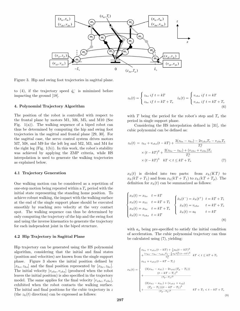
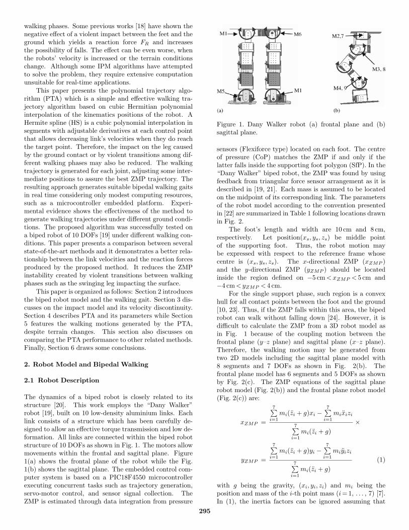
Figure 3. Hip and swing foot trajectories in sagittal plane.

to (4), if the trajectory speed q−e is minimized beforeimpacting the ground [18].

4. Polynomial Trajectory Algorithm

The position of the robot is controlled with respect tothe frontal plane by motors M1, M6, M5, and M10 (SeeFig. 1(a)). The walking sequence of a biped robot canthus be determined by computing the hip and swing foottrajectories in the sagittal and frontal plane [29, 30]. Forthe sagittal case, the servo control system drives motorsM7, M8, and M9 for the left leg and M2, M3, and M4 forthe right leg (Fig. 1(b)). In this work, the robot’s stabilitywas achieved by applying the ZMP criteria, while HSinterpolation is used to generate the walking trajectoriesas explained below.

4.1 Trajectory Generation

One walking motion can be considered as a repetition ofone-step motion being repeated within a Ts period with theinitial state representing the standing home position. Toachieve robust walking, the impact with the walking surfaceat the end of the single support phase should be executedsmoothly by reaching zero velocity at the very contactspot. The walking sequence can thus be determined byonly computing the trajectory of the hip and the swing footand using the inverse kinematics to generate the trajectoryfor each independent joint in the biped structure.

4.2 Hip Trajectory in Sagittal Plane

Hip trajectory can be generated using the HS polynomialalgorithm, considering that the initial and final states(position and velocities) are known from the single supportphase. Figure 3 shows the initial position defined by[xhs, zhs] and the final position represented by [xhe, zhe].The initial velocity [vxhs, vzhs] (produced when the robotleaves the initial position) is also specified in the trajectorymodel. The same applies for the final velocity [vxhe, vzhe],exhibited when the robot contacts the walking surface.The initial and final positions for the cubic trajectory in z(the zh(t) direction) can be expressed as follows:

zh(t) =

⎧⎨⎩

zhs if t = kT

zhe if t = kT + Ts

�zh(t) =

⎧⎨⎩

vzhs if t = kT

vzhe if t = kT + Ts

(6)

with T being the period for the robot’s step and Ts theperiod in single support phase.

Considering the HS interpolation defined in [31], thecubic polynomial can be defined as:

zh(t) = zhs + vzhs(t− kT ) +3(zhe − zhs)− 2vzhsTs − vzheTs

T 2s

× (t− kT )2 +2(zhs − zhe) + (vzhs + vzhe)Ts

T 3s

× (t− kT )3 kT < t ≤ kT + Ts (7)

xh(t) is divided into two parts: from xh(KT) toxh(kT+T1) and from xh(kT+T1) to xh(kT+Tp). Thedefinition for xh(t) can be summarized as follows:

⎧⎪⎪⎪⎪⎪⎪⎨⎪⎪⎪⎪⎪⎪⎩

xh(t) = xhs t = kT

xh(t) = xh1 t = kT + T1

xh(t) = xhe t = kT + Ts

�xh(t) = vxhs t = kT

⎧⎪⎪⎪⎨⎪⎪⎪⎩

�xh(t−) =

.xh(t

+) t = kT + T1

�xh(t) = vxhe t = kT + Ts

xh(t) = a0 t = kT

(8)

with ao being pre-specified to satisfy the initial conditionof acceleration. The cubic polynomial trajectory can thusbe calculated using (7), yielding:

xh(t) =

⎧⎪⎪⎪⎪⎪⎪⎪⎪⎪⎪⎪⎪⎪⎪⎪⎪⎪⎪⎪⎪⎪⎨⎪⎪⎪⎪⎪⎪⎪⎪⎪⎪⎪⎪⎪⎪⎪⎪⎪⎪⎪⎪⎪⎩

xhs + vxhs(t − kT ) + 12a0(t − kT )2

+(xh1−xhs−vxhsT1− 1

2 a0T21 )(t−kT )3

T31

kT < t ≤ kT + T1

xh1 + vxh1(t − kT − T1)

+

(3(xhe − xh1) − 2vxh1(Tp − T1))

(t − kT − T1)2

(Tp−T1)2

+

(2(xh1 − xhe) + (vxh1 + vx2)

(Tp − T1))(t − kT − T1)3

(Tp−T1)3kT + T1 < t − kT + Ts

(9)

297

4.3 Swing Foot Trajectory in Sagittal Plane

HS polynomial interpolation is used to generate the foottrajectory in the single support phase. To assure a smoothtransition, velocities ((vxhs, vzhs) and (vxfe, vzfe)) shouldbe defined near zero. The final foot position (Fig. 3)representing target positions and velocities can thus beobtained following:

xf (t) =

⎧⎪⎪⎪⎪⎪⎪⎨⎪⎪⎪⎪⎪⎪⎩

xf (t) = xfs t = kT

xf (t) = xfe t = kT + Ts

xf (t) = 0 t = kT

xf (t) = 0 t = kT + Ts

zf (t) =

⎧⎪⎪⎪⎪⎪⎪⎨⎪⎪⎪⎪⎪⎪⎩

zf (t) = zfs t = kT

zf (t) = zfe t = kT + Ts

zf (t) = 0 t = kT

zf (t) = 0 t = kT + Ts

(10)

From the initial and the final positions in x- and z-axis, a smooth trajectory can be generated by the HSinterpolation yielding for xf (t) and zf (t):

xf (t) = xfs + 3(xfe − xfs)(t − kT )2

T 2s

−2(xfe − xfs)(t − kT )3

T 3s

kT < t ≤ kT + Ts

zf (t) =

⎧⎪⎪⎪⎪⎪⎪⎪⎪⎪⎨⎪⎪⎪⎪⎪⎪⎪⎪⎪⎩

zfs + 3(zfm − zfs)(t−kT )2

T2m

−2(zfm − zfs)(t−kT )3

T2m

kT < t ≤ kT + Tm

zfm + 3(zfe − zfm) (t−kT−Tm)2

(Ts−Tm)2

−2(zfe − zfm) (t−kT−Tm)3

(Ts−Tm)3kT + Tm < t ≤ kT + Ts

(11)

The hip and knee positions required to produce appro-priate movements for each leg can thus be calculated usingthe inverse kinematics of the robot’s structure.

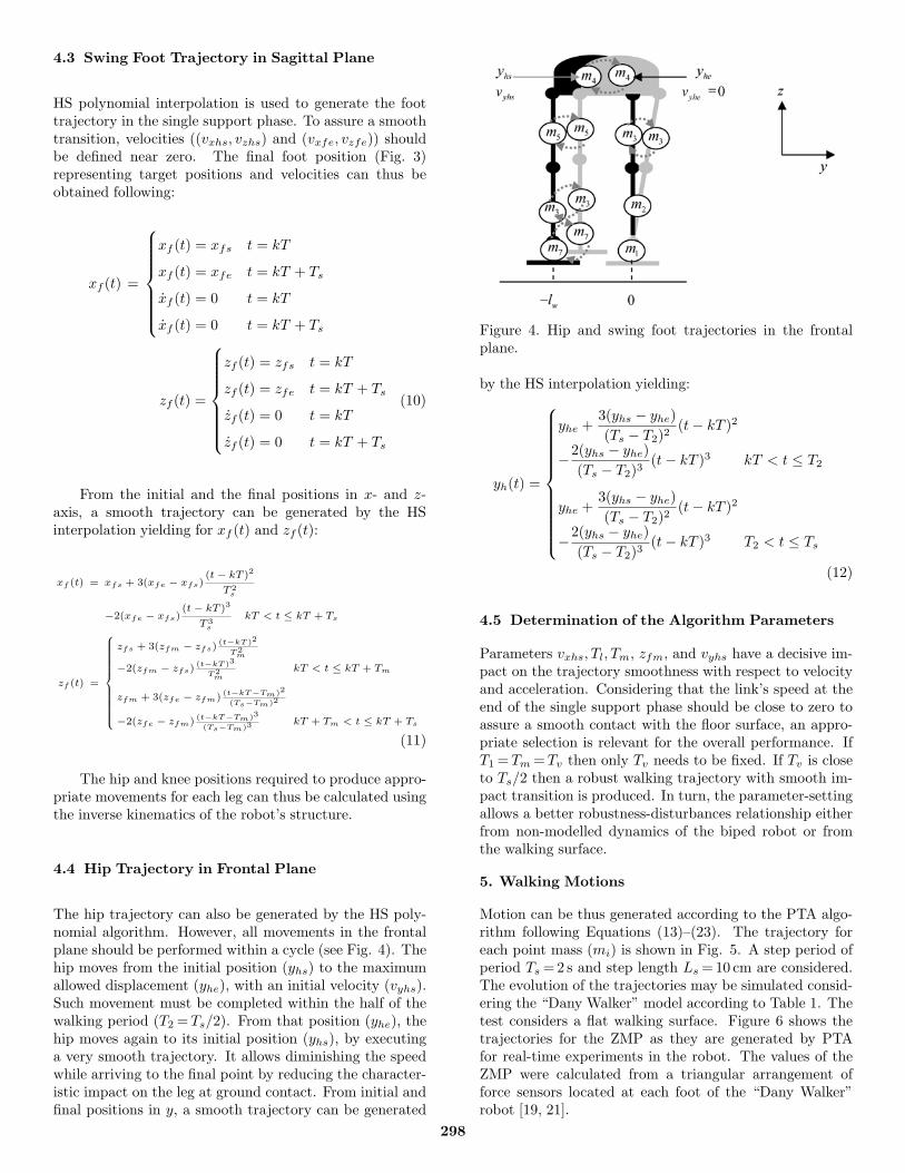
4.4 Hip Trajectory in Frontal Plane

The hip trajectory can also be generated by the HS poly-nomial algorithm. However, all movements in the frontalplane should be performed within a cycle (see Fig. 4). Thehip moves from the initial position (yhs) to the maximumallowed displacement (yhe), with an initial velocity (vyhs).Such movement must be completed within the half of thewalking period (T2 =Ts/2). From that position (yhe), thehip moves again to its initial position (yhs), by executinga very smooth trajectory. It allows diminishing the speedwhile arriving to the final point by reducing the character-istic impact on the leg at ground contact. From initial andfinal positions in y, a smooth trajectory can be generated

Figure 4. Hip and swing foot trajectories in the frontalplane.

by the HS interpolation yielding:

yh(t) =

⎧⎪⎪⎪⎪⎪⎪⎪⎪⎪⎪⎪⎨⎪⎪⎪⎪⎪⎪⎪⎪⎪⎪⎪⎩

yhe +3(yhs − yhe)

(Ts − T2)2(t− kT )2

−2(yhs − yhe)

(Ts − T2)3(t− kT )3 kT < t ≤ T2

yhe +3(yhs − yhe)

(Ts − T2)2(t− kT )2

−2(yhs − yhe)

(Ts − T2)3(t− kT )3 T2 < t ≤ Ts

(12)

4.5 Determination of the Algorithm Parameters

Parameters vxhs, Tl, Tm, zfm, and vyhs have a decisive im-pact on the trajectory smoothness with respect to velocityand acceleration. Considering that the link’s speed at theend of the single support phase should be close to zero toassure a smooth contact with the floor surface, an appro-priate selection is relevant for the overall performance. IfT1 =Tm =Tv then only Tv needs to be fixed. If Tv is closeto Ts/2 then a robust walking trajectory with smooth im-pact transition is produced. In turn, the parameter-settingallows a better robustness-disturbances relationship eitherfrom non-modelled dynamics of the biped robot or fromthe walking surface.

5. Walking Motions

Motion can be thus generated according to the PTA algo-rithm following Equations (13)–(23). The trajectory foreach point mass (mi) is shown in Fig. 5. A step period ofperiod Ts =2 s and step length Ls =10 cm are considered.The evolution of the trajectories may be simulated consid-ering the “Dany Walker” model according to Table 1. Thetest considers a flat walking surface. Figure 6 shows thetrajectories for the ZMP as they are generated by PTAfor real-time experiments in the robot. The values of theZMP were calculated from a triangular arrangement offorce sensors located at each foot of the “Dany Walker”robot [19, 21].

298

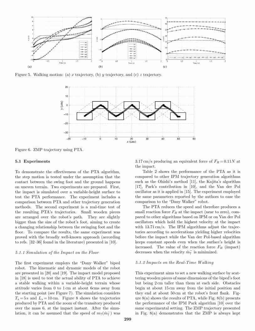
Figure 5. Walking motion: (a) x trajectory, (b) y trajectory, and (c) z trajectory.

Figure 6. ZMP trajectory using PTA.

5.1 Experiments

To demonstrate the effectiveness of the PTA algorithm,the step motion is tested under the assumption that thecontact between the swing foot and the ground happenson uneven terrain. Two experiments are prepared. First,the impact is simulated over a variable-height surface totest the PTA performance. The experiment includes acomparison between PTA and other trajectory generationmethods. The second experiment is a real-time test ofthe resulting PTA’s trajectories. Small wooden piecesare arranged over the robot’s path. They are slightlybigger than the size of the robot’s foot, aiming to createa changing relationship between the swinging foot and thefloor. To compare the results, the same experiment wasproved with the broadly well-known approach (accordingto refs. [32–36] found in the literature) presented in [10].

5.1.1 Simulation of the Impact on the Floor

The first experiment employs the “Dany Walker” bipedrobot. The kinematic and dynamic models of the robotare presented in [20] and [19]. The impact model proposedin [18] is used to test the actual ability of PTA to achievea stable walking within a variable-height terrain whoseattitude varies from 0 to 1 cm at about 6cms away fromthe starting point (see Figure 7). The simulation considersTs =5 s and Ls =10 cm. Figure 8 shows the trajectoriesproduced by PTA and the zoom of the transitory producedover the mass 6, at the impact instant. After the simu-lation, it can be assumed that the speed of m7(m

−7 ) was

3.17 cm/s producing an equivalent force of FR =0.11N atthe impact.

Table 2 shows the performance of the PTA as it iscompared to other IPM trajectory generation algorithmssuch as the Ohishi’s method [11], the Kajita’s algorithm[17], Park’s contribution in [10], and the Van der Poloscillator as it is applied in [15]. The experiment employedthe same parameters reported by the authors to ease thecomparison to the “Dany Walker” robot.

The PTA reduces the speed and therefore produces asmall reaction force FR at the impact (near to zero), com-pared to other algorithms based on IPM or on Van der Poloscillators which hold the highest velocity at the impactwith 13.71 cm/s. The IPM algorithms adjust the trajec-tories according to accelerations yielding higher velocitiesbefore the impact while the Van der Pol-based algorithmkeeps constant speeds even when the surface’s height isincreased. The value of the reaction force FR (impact)decreases when the velocity m−

7 is minimized.

5.1.2 Impacts on the Real-Time Walking

This experiment aims to set a new walking surface by scat-tering wooden pieces of same dimensions of the biped’s footbut being 2 cm taller than them at each side. Obstaclesbegin at about 15 cm away from the initial position andthey end at about 50 cm at the robot’s front flank. Fig-ure 8(a) shows the results of PTA, while Fig. 8(b) presentsthe performance of the IPM Park algorithm [10] over thesame experimental setting. The ZMP trajectory presentedin Fig. 8(a) demonstrates that the ZMP is always kept

299

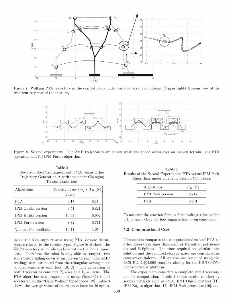
Figure 7. Walking PTA trajectory in the sagittal plane under variable terrain conditions. (Upper right) A zoom view of thetransient response of the mass m6.

Figure 8. Second experiment. The ZMP trajectories are shown while the robot walks over an uneven terrain. (a) PTAoperation and (b) IPM Park’s algorithm.

Table 2Results of the First Experiment: PTA versus OtherTrajectory Generation Algorithms under Changing

Terrain Conditions

Algorithms Velocity of m7 (m−7 ) FR (N)

(cm/s)

PTA 3.17 0.11

IPM Ohishi version 9.51 0.821

IPM Kajita version 10.44 0.902

IPM Park version 8.82 0.711

Van der Pol oscillator 13.71 1.05

inside the foot support area using PTA, despite distur-bances related to the terrain type. Figure 8(b) shows theZMP trajectory is not always kept within the foot supportarea. Therefore, the robot is only able to complete twosteps before falling down at an uneven terrain. The ZMPreadings were estimated from the triangular arrangementof force sensors at each foot [19, 21]. The generation ofboth trajectories considers Ts =5 s and Ls =10 cm. ThePTA algorithm was programmed using Visual C++ andwas tested on the “Dany Walker” biped robot [19]. Table 3shows the average values of the reaction force for 20 cycles.

Table 3Results of the Second Experiment: PTA versus IPM Park

Algorithms under Changing Terrain Conditions

Algorithms FR (N)

IPM Park version 0.717

PTA 0.201

To measure the reaction force, a force–voltage relationship[37] is used. Only left foot impacts have been considered.

5.2 Computational Cost

This section compares the computational cost of PTA toother generation algorithms such as Hermitian polynomi-als and B-Splines. The time required to calculate thesolution and the required storage space are considered ascomparison indexes. All systems are compiled using theCCS PIC-C r©4.068 compiler aiming for the PIC18F4550microcontroller platform.

The experiment considers a complete step trajectoryand its computation. Table 4 shows results consideringseveral methods such as PTA, IPM Ohishi method [11],IPM Kajita algorithm [17], IPM Park procedure [10], and

300

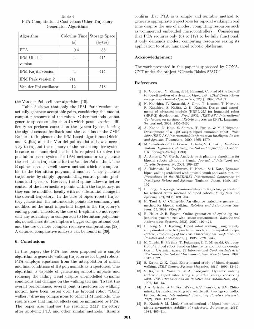
Table 4PTA Computational Cost versus Other Trajectory

Generation Algorithms

Algorithm Calculus Time Storage Space

(s) (bytes)

PTA 0.4 86

IPM Ohishi 4 415

version

IPM Kajita version 4 415

IPM Park version 2 211

Van der Pol oscillator 12 518

the Van der Pol oscillator algorithm [15].Table 3 shows that only the IPM Park version can

actually generate acceptable gaits, considering the modestcomputer resources of the robot. Other methods cannotgenerate speeds smaller than 4 s which poses a serious dif-ficulty to perform control on the system by consideringthe signal sensors feedback and the calculus of the ZMP.Besides, to implement the IPM-based algorithms (Ohishi,and Kajita) and the Van del pol oscillator, it was neces-sary to expand the memory of the host computer systembecause one numerical method is required to solve thependulum-based system for IPM methods or to generatethe oscillation trajectories for the Van der Pol method. TheB-splines class is a well-known method which is compara-ble to the Hermitian polynomial models. They generatetrajectories by simply approximating control points (posi-tions and speeds). However, the B-spline allows a bettercontrol of the intermediate points within the trajectory, asthey can be modified locally with no substantial change inthe overall trajectory. In the case of biped-robots trajec-tory generation, the intermediate points are commonly notmodified as the most important target is the trajectory’sending point. Therefore, the use of B-splines do not repre-sent any advantage in comparison to Hermitian polynomi-als, nonetheless its use implies a bigger computational costand the use of more complex recursive computations [38].A detailed comparative analysis can be found in [39].

6. Conclusions

In this paper, the PTA has been proposed as a simplealgorithm to generate walking trajectories for biped robots.PTA employs equations from the interpolation of initialand final conditions of HS polynomials as trajectories. Thealgorithm is capable of generating smooth impacts andreducing the falling trend despite un-modelled dynamicconditions and changes on the walking terrain. To test theoverall performance, several joint trajectories for walkingmotion have been tested over the bipedal robot “Danywalker,” drawing comparisons to other IPM methods. Theresults show that impact effects can be minimized by PTA.The paper also analyses the resulting ZMP trajectoryafter applying PTA and other similar methods. Results

confirm that PTA is a simple and suitable method togenerate appropriate trajectories for bipedal walking in realtime despite the use of modest computing resources suchas commercial embedded microcontrollers. Consideringthat PTA requires only (6) to (12) to be fully functional,it only demands modest computing resources easing itsapplication to other humanoid robotic platforms.

Acknowledgement

The work presented in this paper is sponsored by CONA-CYT under the project “Ciencia Basica 82877.”

References

[1] R. Goddard, Y. Zheng, & H. Hemami, Control of the heel-offto toe-off motion of a dynamic biped gait, IEEE Transactionson Systems Manard Cybernetics, 22(1), 1992, 92–102.

[2] N. Kanehira, T. Kawasaki, S. Ohta, T. Isozumi, T. Kawada,F. Kanehiro, S. Kajita, & K. Kaneko, Design and experi-ments of advanced module (HRPL-2L) for humanoid robot(HRP-2) development, Proc. 2002, IEEE-RSJ InternationalConference on Intelligent Robote and System EPFL, Lausanne,Switzerland, 2002, 2455–2460.

[3] A. Konno, N. Kato, S. Shirata, T. Furuta, & M. Uchiyama,Development of a light-weight biped humanoid robot, Proc.2000 IEEE-RSJ International Conference on Intelligent Roboteand Systems, Takamatsu, 2000, 1565–1570.

[4] M. Vukobratovic, B. Borovac, D. Surla, & D. Stokic, Biped loco-motion: Dynamics, stability, control and application (London,UK: Springer-Verlag, 1990).

[5] A. Amos & W. Gerth, Analytic path planning algorithms forbipedal robots without a trunk, Journal of Intelligent andRobotic Systems, 36, 2003, 109–127.

[6] A. Takanishi, M. Tochizawa, H. Karaki, & I. Kato, Dynamicbiped walking stabilized with optimal trunk and waist motion,Proceedings of the IEEE/RSJ International Conference onIntelligent Robots and Systems, Tsukuba, Japan, 1989, 187–192.

[7] H. Jong, Fuzzy-logic zero-moment-point trajectory generationfor reduced trunk motions of biped robots, Fuzzy Sets andSystems, 134, 2003, 189–203.

[8] H. Taesi & C. Chong-Ho, An effective trajectory generationmethod for bipedal walking, Robotics and Autonomous Sys-tems, 55, 2007, 795–810.

[9] R. Heliot & B. Espiau, Online generation of cyclic leg tra-jectories synchronized with sensor measurement, Robotics andAutonomous Systems, 56(3), 2007, 410–421.

[10] H. Jong & D. Kyoung, Biped robot walking using gravitycompensated inverted pendulum mode and computed torquecontrol, Proceedings of the IEEE International Conference onRobotics and Automation, 4, 1998, 3528–3533.

[11] K. Ohishi, K. Majima, T. Fukunaga, & T. Miyazaki, Gait con-trol of a biped robot based on kinematics and motion descrip-tion in Cartesian space, 23 International Conf. on IndustrialElectronics, Control and Instrumentation, New Orleans, 1997,1317–1322.

[12] S. Kajita & K. Tani, Experimental study of biped dynamicwalking, IEEE Control Systems Magazine, 16(1), 1996, 13–19.

[13] S. Kajita, T. Yamaura, & A. Kobayashi, Dynamic walkingcontrol of biped robot along a potential energy conservingorbit, IEEE Transactions on Robotics and Automation, 8(4),1992, 431–437.

[14] A.A. Grishin, A.M. Formal’sky, A.V. Lensky, & S.V. Zhito-mirsky, Dynamical walking of a vehicle with two legs controlledby two drives, International Journal of Robotics Research,13(2), 1994, 137–147.

[15] R. Katoh & M. Mori, Control method of biped locomotiongiving asymptotic stability of trajectory. Automatica, 20(4),1984, 405–414.

301

[16] J. Furusho & M. Masubuchi, Control of a dynamical bipedlocomotion system for steady walking. Journal of DynamicSystems, Measurement and Control, 108, 1986, 111–118.

[17] S. Kajita, F. Kanehiro, K. Kaneko, K. Fijiware, K. Harada,K. Yokoi, & H. Hirukawa, Biped walking pattern generationby using preview control of zero-moment point, IEEE Inter-national Conference on Robotics and Automation, 2, 2003,1620–1626.

[18] Y. Hurmuzlu & D.B. Marghitu, Rigid body collisions of planarkinematic chains with multiple contact points, InternationalJournal of Robotics Research, 13(1), 1994, 82–92.

[19] D. Zaldivar, A biped robot design, Doctoral Dissertation, Fach-bereich Mathematik u. Informatik, Freie Universitat Berlin,Berlin, 2006.

[20] E. Cuevas, D. Zaldıvar, & R. Rojas, Bipedal robot description,Technical Report B-03-19, Freie Universitat Berlin, FachbereichMathematik und Informatik, Berlin, Germany, 2004.

[21] K. Erbatur, A. Okazaki, K. Obiya, T. Takahashi, & A.Kawamura, A study on the zero moment point measurementfor biped walking robots, IEEE 7th International Workshopon Advanced Motion Control, Istanbul, 2002, 431–436.

[22] K. Qiang Huang, S. Yokoi, K. Kajita, H. Kaneko, N. Arai,& K. Koyachi, Planning walking patterns for a biped robot,IEEE Transactions on Robotics and Automation, 17, 2001,280–289.

[23] A. Yonemura, Y. Nakajima, A.R. Hirakawa, & A. Kawamura,Experimental approach for the biped walking robot MARI-1,6th International Workshop on Advanced Motion Control,Nagoya, 2000, 548–553.

[24] D. Katic & M. Vukobratovic, Survey of intelligent controltechniques for humanoid robots, Journal of Intelligent andRobotic Systems, 37, 2003, 117–141.

[25] S. Czarnetzki, S. Kernera, & O. Urbanna, Observer-baseddynamic walking control for biped robots, Robotics and Au-tonomous Systems 57(8), 2009, 839–845.

[26] E. Westervelt, J. Grizzle, C. Chevallerau, J Choi, & B. Morris,Feedback control of dynamic bipedal robot locomotion, (NW:CRC Press, 2007).

[27] B. Brogliato, Nonsmooth impact dynamics: models, dynamicsand control, (London: Springer, 1996).

[28] Y. Fujimoto & A. Kawamura, Simulation of an autonomousbiped walking robot including environmental force interaction,IEEE Robotics and Automation Magazine, 5(2), 1998, 33–42.

[29] A. Takanishi, M. Ishida, Y. Yamazaki, & I. Kato, The real-ization of dynamic walking by the biped walking robot, Proc.of International Conference on Advanced Robotics, St. Louis,MO, 1985, 459–466.

[30] K. Hiria, M Hirose, Y. Haikawa, & T. Takenaka, The develop-ment of Honda humanoid robot, IEEE International Confer-ence on Robotics and Automation, Leuven, 1998, 1321–1326.

[31] M. Fedoryuk, Hermite polynomials: Encyclopedia of mathe-matics (Holland: Kluwer Academic Publishers, 2001).

[32] K. Nishiwaki & S. Kagami, Online walking control for hu-manoids with short cycle pattern generation, The InternationalJournal of Robotics Research, 28, 2009, 729–742.

[33] S. Bououden, F. Abdessemed, & B. Abderraouf, Control ofa bipedal walking robot using a fuzzy precompensator, inA. Hakansson et al. (Eds.), Agent and multi-agent systems:Technologies and applications (Berlin: Springer-Verlag, 2009),1344–1370.

[34] C. Zeng, Y. Cheng, H. Liang, L. Dai, & H. Liu, Research onthe model of the inverted pendulum and its control based onbiped robot, IEEE Pacific-Asia Workshop on Computationaland Industrial Application, Wuhan, 2008, 100-103

[35] J. Park, Fuzzy-logic zero moment point trajectory generationfor reduced trunk motions of biped robots, Fuzzy Sets andSystems, 134, 2003, 189–203.

[36] S. Kajita, F. Kanehiro, K. Kaneko, & K. Fujiwara, A real-time Pattern generation for a Biped Walking, InternationalConference on Robotics & Automation, 1, Washington, DC,2002, 31–37.

[37] http://www.tekscan.com/flexiforce/flexiforce.html.[38] T. Popiel, On parametric smoothness of generalised B-spline

curves, Computer Aided Geometric Design, 23(8), 2006, 655–668.

[39] M. Unser, A. Aldroubi, & M. Eden, Fast B-spline transformsfor continuos image representation and interpolation, IEEETransactions On Pattern Analysis and Machine Intelligence,13(3), 1991, 277–285.

Biographies

Erik Cuevas received his B.S.degree with distinction in Elec-tronics and Communications En-gineering from the University ofGuadalajara, Mexico, in 1995,the M.Sc. degree in IndustrialElectronics from ITESO, Mexico,in 2000, and the Ph.D. degreefrom Freie Universitat Berlin,Germany, in 2005. Since 2001, hewas awarded a scholarship fromthe German Service for Academic

Interchange (DAAD) as full-time researcher. From 2006he has been with University of Guadalajara, where heis currently a full-time professor in the Department ofComputer Science. From 2008, he is also a member of theMexican National Research System (SNI). His researchinterest includes computer vision and artificial intelligenceapplications in medical image.

Daniel Zaldivar received hisB.S. degree with distinction inElectronics and CommunicationsEngineering from the Universityof Guadalajara, Mexico, in 1995,the M.Sc. degree in IndustrialElectronics from ITESO, Mexico,in 2000, and the Ph.D. degreefrom Freie Universitat Berlin,Germany, in 2005. From 2001 hewas awarded a scholarship fromthe German Service for Academic

Interchange (DAAD) as full-time researcher. From 2006he has been with University of Guadalajara, where heis currently a professor in the Department of ComputerScience. From 2008 he is also a member of the MexicanNational Research System (SNI). His current researchinterest includes biped robots design, humanoid walkingcontrol, and artificial vision.

Marco Perez-Cisneros receivedhis B.S. degree with distinction inElectronics and CommunicationsEngineering fromtheUniversity ofGuadalajara, Mexico, in 1995, theM.Sc. degree in Industrial Elec-tronics from ITESO University,Mexico, in 2000, and the Ph.D.degree from the Control SystemsCentre, UMIST,Manchester, UK,in 2004. From 2005 he has beenwith University of Guadalajara,

302

where he is currently a professor and head of Departmentof Computer Science. From 2007 he has spent yearly spellsat the University of Manchester as an invited honorary pro-fessor. He is a member of the Mexican National ResearchSystem (SNI) since 2007. His current research interestincludes robotics and computer vision in particular visualservoing applications on humanoid walking control.

Marte Ramırez-Ortegon is aPh.D. student at the Departmentof Mathematics and ComputerScience of the Freie UniversitatBerlin. In 2002, he received a B.S.degree (Computer Science) fromthe University of Guanajuato(UG)/the Centre for Mathemat-ical Research (CIMAT), Guana-juato, Mexico (1998–2002). Hiscurrent research fields include pat-tern recognition, edge detection,

binarization, multithresholding, and text recognition.

303