Polynomial Decomposition Algorithms in Signal Processing by Guolong Su B.Eng., Electronic Engineering, Tsinghua University, China (2011) Submitted to the Department of Electrical Engineering and Computer Science in partial fulfillment of the requirements for the degree of Master of Science in Electrical Engineering and Computer Science at the MASSACHUSETTS INSTITUTE OF TECHNOLOGY June 2013 c Massachusetts Institute of Technology 2013. All rights reserved. Author .............................................................. Department of Electrical Engineering and Computer Science May 20, 2013 Certified by .......................................................... A. V. Oppenheim Ford Professor of Engineering Thesis Supervisor Accepted by ......................................................... Professor Leslie A. Kolodziejski Chairman, Department Committee on Graduate Theses

Welcome message from author
This document is posted to help you gain knowledge. Please leave a comment to let me know what you think about it! Share it to your friends and learn new things together.
Transcript

Polynomial Decomposition Algorithms in Signal
Processing
by
Guolong Su
B.Eng., Electronic Engineering, Tsinghua University, China (2011)
Submitted to the Department of Electrical Engineering and ComputerScience
in partial fulfillment of the requirements for the degree of
Master of Science in Electrical Engineering and Computer Science
at the
MASSACHUSETTS INSTITUTE OF TECHNOLOGY
June 2013
c© Massachusetts Institute of Technology 2013. All rights reserved.
Author . . . . . . . . . . . . . . . . . . . . . . . . . . . . . . . . . . . . . . . . . . . . . . . . . . . . . . . . . . . . . .Department of Electrical Engineering and Computer Science
May 20, 2013
Certified by. . . . . . . . . . . . . . . . . . . . . . . . . . . . . . . . . . . . . . . . . . . . . . . . . . . . . . . . . .A. V. Oppenheim
Ford Professor of Engineering
Thesis Supervisor
Accepted by . . . . . . . . . . . . . . . . . . . . . . . . . . . . . . . . . . . . . . . . . . . . . . . . . . . . . . . . .
Professor Leslie A. KolodziejskiChairman, Department Committee on Graduate Theses

2
Polynomial Decomposition Algorithms in Signal Processing
by
Guolong Su
Submitted to the Department of Electrical Engineering and Computer Scienceon May 20, 2013, in partial fulfillment of the
requirements for the degree ofMaster of Science in Electrical Engineering and Computer Science
Abstract
Polynomial decomposition has attracted considerable attention in computational math-ematics. In general, the field identifies polynomials f(x) and g(x) such that theircomposition f(g(x)) equals or approximates a given polynomial h(x). Despite po-tentially promising applications, polynomial decomposition has not been significant-ly utilized in signal processing. This thesis studies the sensitivities of polynomialcomposition and decomposition to explore their robustness in potential signal pro-cessing applications and develops effective polynomial decomposition algorithms tobe applied in a signal processing context. First, we state the problems of sensitivity,exact decomposition, and approximate decomposition. After that, the sensitivitiesof the composition and decomposition operations are theoretically derived from theperspective of robustness. In particular, we present and validate an approach to de-crease certain sensitivities by using equivalent compositions, and a practical rule forparameter selection is proposed to get to a point that is near the minimum of thesesensitivities. Then, new algorithms are proposed for the exact decomposition prob-lems, and simulations are performed to make comparison with existing approaches.Finally, existing and new algorithms for the approximate decomposition problems arepresented and evaluated using numerical simulations.
Thesis Supervisor: A. V. OppenheimTitle: Ford Professor of Engineering
3

4

Acknowledgments
I would like to first thank my research advisor Prof. Alan Oppenheim, whose re-
markable wisdom and guidance for this thesis are significant in many ways. I am
deeply impressed by Al’s unconventional creativity, and I am particularly thankful
for our research meetings that were not only academically invaluable but also emo-
tionally supportive. Al is a great source of sharp and insightful ideas and comments,
which make me always feel more energetic to explore more stimulating directions after
meeting with him. I am also sincerely grateful to Al, a great mentor, for patiently im-
proving my academic writing level and shaping me into a person with higher maturity.
In addition to his tremendous intellectual support, I really appreciate Al’s impressive
warmheartedness and caring efforts in helping me with a number of personal issues
to make my life comfortable at MIT and during the summer internship.
I would also like to thank Sefa Demirtas for his helpful contribution and our
friendly research collaboration during the last two years. The topic of this thesis
had been discovered by Al and Sefa before I joined MIT; Sefa has been a great
close collaborator with a significant role in the development of many results in this
thesis. In addition, I sincerely thank Sefa for carefully reviewing the thesis and
patiently helping me with other English documents. I am also grateful to Sefa for his
enthusiastic encouragement, guidance and support.
It has been an enjoyable and rewarding journey for me as a member of Digital
Signal Processing Group (DSPG). I would like to sincerely thank the past and present
DSPG members including: Tom Baran, Petros Boufounos, Sefa Demirtas, Dan Dud-
geon, Xue Feng, Yuantao Gu, Zahi Karam, Tarek Lahlou, Martin McCormick, Milutin
Pajovic, Charlie Rohrs, and Laura von Bosau. The collaborative research environ-
ment and the intriguing weekly brainstorming meetings make the group an enthu-
siastic, creative, and harmonious academic family. Especially, thanks to Laura for
her responsible efforts to make the group function efficiently and constant readiness
to help; thanks to Tarek for his enthusiastic conversation in the night when we both
heard for the first time of the problem of polynomial decomposition as well as his
5

helpful comments as a native speaker on my English documents; thanks to Zahi for
the helpful discussion on root-finding algorithms; thanks to Yuantao for the enthu-
siastic discussion on Vandermonde matrices as well as your valuable guidance and
friendly mentorship during my time in Tsinghua University. In addition to group
members, I would thank Yangqin for the helpful discussion on the Galois group.
I would also like to thank Davis Pan at Bose Corporation. Davis is a great and
easygoing manager, who is truly caring about his interns even beyond the scope of
the internship. The experience with Davis was really enjoyable both intellectually
and personally.
I feel really fortunate to have met and been accompanied by Shengxi. I thank her
for her companionship, kind heart, patience, as well as the love and happiness she
has brought me. Special thanks for her encouragement for going to the gym and her
correction of my English pronunciation.
I am deeply grateful to my parents for their unconditional love and unlimited
support. Through the years, I know that they are always available to talk to for
support and encouragement. Their guidance and wisdom in life have been essential
for the development of my personality. My love and appreciation for my parents is
beyond any words. Thanks also to my extended family for their love and support
when I am far away from home.
6

Contents
1 Introduction 13
1.1 Motivation . . . . . . . . . . . . . . . . . . . . . . . . . . . . . . . . . 13
1.2 Objective . . . . . . . . . . . . . . . . . . . . . . . . . . . . . . . . . 15
2 Background 17
2.1 Polynomial Composition Properties . . . . . . . . . . . . . . . . . . . 17
2.2 Review of Existing Polynomial Decomposition Algorithms . . . . . . 19
3 Problem Definition 21
3.1 Sensitivity Analysis . . . . . . . . . . . . . . . . . . . . . . . . . . . . 21
3.1.1 Sensitivities of the Coefficients . . . . . . . . . . . . . . . . . . 22
3.1.2 Sensitivities of the Roots . . . . . . . . . . . . . . . . . . . . . 23
3.2 Exact Decomposition . . . . . . . . . . . . . . . . . . . . . . . . . . . 25
3.3 Approximate Decomposition . . . . . . . . . . . . . . . . . . . . . . . 27
4 Sensitivities of Polynomial Composition and Decomposition 29
4.1 Derivation of the Sensitivities . . . . . . . . . . . . . . . . . . . . . . 29
4.1.1 Sensitivities of the Coefficients . . . . . . . . . . . . . . . . . . 29
4.1.2 Sensitivities of the Roots . . . . . . . . . . . . . . . . . . . . . 33
4.2 Sensitivities of Equivalent Compositions with First-Degree Polynomials 38
4.3 Simulation Results . . . . . . . . . . . . . . . . . . . . . . . . . . . . 43
4.3.1 Evaluation of the Sensitivities . . . . . . . . . . . . . . . . . . 43
4.3.2 Comparisons of the Sensitivities . . . . . . . . . . . . . . . . . 48
7

4.3.3 Sensitivities of Equivalent Compositions . . . . . . . . . . . . 49
5 Exact Decomposition Algorithms 55
5.1 Problem 1: Exact Decomposition with Coefficients as Input . . . . . 56
5.2 Problem 2: Exact Decomposition with Roots as Input . . . . . . . . . 58
5.2.1 Properties of Roots of a Decomposable Polynomial . . . . . . 58
5.2.2 Root-Power-Summation Algorithm . . . . . . . . . . . . . . . 59
5.2.3 Root-Grouping Algorithm . . . . . . . . . . . . . . . . . . . . 60
5.3 Evaluation of the Exact Decomposition Algorithms . . . . . . . . . . 63
6 Approximate Decomposition Algorithms 69
6.1 Problem 3: Approximate Decomposition with Coefficients as Input . 69
6.1.1 Iterative Mean Square Approximation Algorithm . . . . . . . 70
6.1.2 Algorithms Based on the Ruppert Matrix . . . . . . . . . . . 71
6.2 Problem 4: Approximate Decomposition with Roots as Input . . . . . 78
6.3 Evaluation of the Approximate Decomposition Algorithms . . . . . . 83
6.3.1 Iterative Mean Square Algorithm . . . . . . . . . . . . . . . . 84
6.3.2 RiSVD Heuristic and STLS Relaxation . . . . . . . . . . . . . 85
6.3.3 Approximate Root-Grouping Algorithm . . . . . . . . . . . . . 87
7 Conclusions and Future Work 89
A Minimum Phase Decomposition for a Minimum Phase Decompos-
able Polynomial 93
B Derivation of Upper Bound (4.13) 99
C Explanation of the Approximate Rules (4.39)-(4.41) for Parameter
Selection 101
8
List of Figures
1-1 Two Implementations of a Decomposable FIR Filter where H(z−1) =
(F ◦G)(z−1) . . . . . . . . . . . . . . . . . . . . . . . . . . . . . . . . 16
4-1 Coefficient Sensitivity from f(x) to h(x). . . . . . . . . . . . . . . . . 44
4-2 Coefficient Sensitivity from h(x) to f(x). . . . . . . . . . . . . . . . . 44
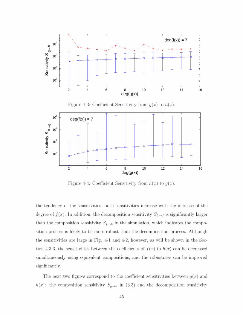
4-3 Coefficient Sensitivity from g(x) to h(x). . . . . . . . . . . . . . . . . 45
4-4 Coefficient Sensitivity from h(x) to g(x). . . . . . . . . . . . . . . . . 45
4-5 Root Sensitivity from zf to zh. . . . . . . . . . . . . . . . . . . . . . . 46
4-6 Root Sensitivity from zh to zf . . . . . . . . . . . . . . . . . . . . . . . 46
4-7 Root Sensitivity from g(x) to zh. . . . . . . . . . . . . . . . . . . . . 47
4-8 Root Sensitivity from zh to g(x). . . . . . . . . . . . . . . . . . . . . 47
4-9 Comparison between Corresponding Coefficient Sensitivities and Root
Sensitivities. . . . . . . . . . . . . . . . . . . . . . . . . . . . . . . . 49
4-10 The Condition Number cond(G) with Different q1 and qr, where qr =q0q1. 50
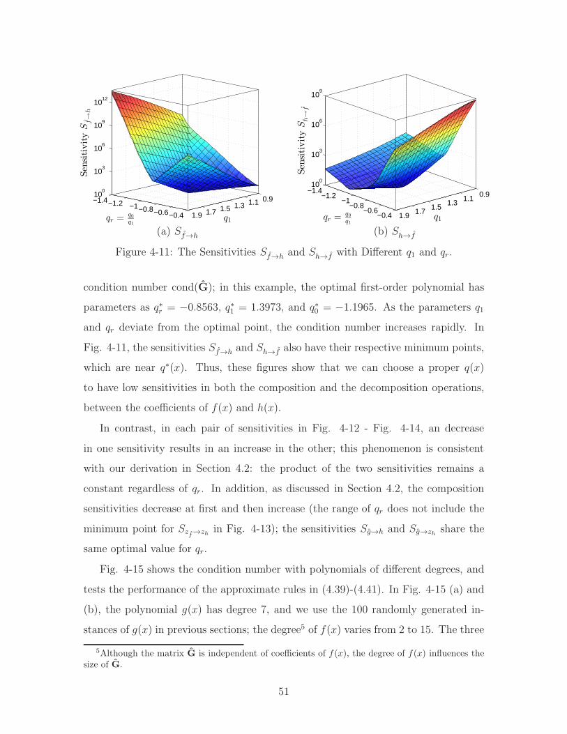
4-11 The Sensitivities Sf→h and Sh→f with Different q1 and qr. . . . . . . . 51
4-12 The Sensitivities Sg→h and Sh→g with Different qr. . . . . . . . . . . . 53
4-13 The Sensitivities Szf→zh and Szh→z
fwith Different qr. . . . . . . . . . 53
4-14 The Sensitivities Sg→zh and Szh→g with Different qr. . . . . . . . . . . 53
4-15 Comparison of the Condition Number of G among the Original Value,
the Minimum Value, and the Value Achieved with the Approximate
Rules (4.39)-(4.41). . . . . . . . . . . . . . . . . . . . . . . . . . . . 54
5-1 Comparison between the three exact decomposition algorithms on the
Success Rates of (a) f(x), (b) g(x), and (c) h(x). . . . . . . . . . . . 67
9

10

List of Tables
3.1 Definitions of the Sensitivities within the Coefficient Triplet (f, g, h) 24
3.2 Definitions of the Sensitivities within the Root Triplet (zf , g, zh) . . 25
6.1 Success Rate of the Iterative Mean Square Algorithm (%) . . . . . . . 85
6.2 Success Rate of the Approximate Decomposition Methods that are
Based on Ruppert Matrix (%) . . . . . . . . . . . . . . . . . . . . . . 86
6.3 Success Rate of the Root Grouping Algorithm for Approximate De-
composition (%) . . . . . . . . . . . . . . . . . . . . . . . . . . . . . . 88
11

12
Chapter 1
Introduction
1.1 Motivation
Functional composition (α ◦ β)(x) is defined as (α ◦ β)(x) = α(β(x)), where α(x)
and β(x) are arbitrary functions. It can be interpreted as a form of cascading the
two functions β(·) and α(·). One application of functional composition in signal
processing is in time warping [1–3]. The basic idea of time warping is to replace the
time variable t with a warping function ψ(t), so the time-axis is stretched in some
parts and compressed in other parts. In this process, a signal s(t) is time-warped to
a new signal s(ψ(t)) in the form of functional composition. It is possible that the
original signal s(t) is non-bandlimited, while the composed signal s(ψ(t)) is band-
limited [1–3]. For example, the chirp signal s(t) = cos(at2) is non-bandlimited [4],
but it can be warped into the band-limited signal s(ψ(t)) = cos(at) by the warping
function ψ(t) =√|t|. For certain signals, if proper warping functions are chosen,
time warping may serve as an anti-aliasing technique in sampling. In addition to
its application in efficient sampling, time warping has also been employed to model
and compensate for certain nonlinear systems [5]. Moreover, time warping may be
utilized in speech recording to improve speech verification [6].
As a particular case of functional composition, polynomial composition may also
find potentially beneficial applications in signal processing. The precise definition of
polynomial composition is stated as follows with the symbols to be used throughout
13
this thesis. For polynomials
f(x) =
M∑
m=0
amxm, g(x) =
N∑
n=0
bnxn, (1.1)
their composition is defined as
h(x) = (f ◦ g)(x) = f(g(x)) =M∑
m=0
am(g(x))m =
MN∑
k=0
ckxk. (1.2)
If a polynomial h(x) can be expressed in form (1.2), then it is decomposable; otherwise
it is indecomposable. For simplicity, we assume that all polynomials f(x), g(x), and
h(x) have real coefficients; however, most results of this thesis also apply for complex
polynomials.
The inverse process to polynomial composition is called polynomial decomposi-
tion, which generally means determining f(x) and g(x) given h(x). Polynomial de-
composition is potentially as useful as composition in signal processing applications.
For example, polynomial decomposition may be employed in efficient representation
of signals [7]. If a signal can be represented by a decomposable polynomial h(x),
then it can also be represented by its decomposition (f ◦ g)(x). Note that h(x) has
(MN + 1) degrees of freedom, while f(x) and g(x) together have degrees of freedom
(M +N). 1 Thus, the decomposition representation of the signal has a reduction of
(MN + 1 −M − N) degrees of freedom and thus can potentially be used for signal
compression. Another possible application of polynomial decomposition is an alter-
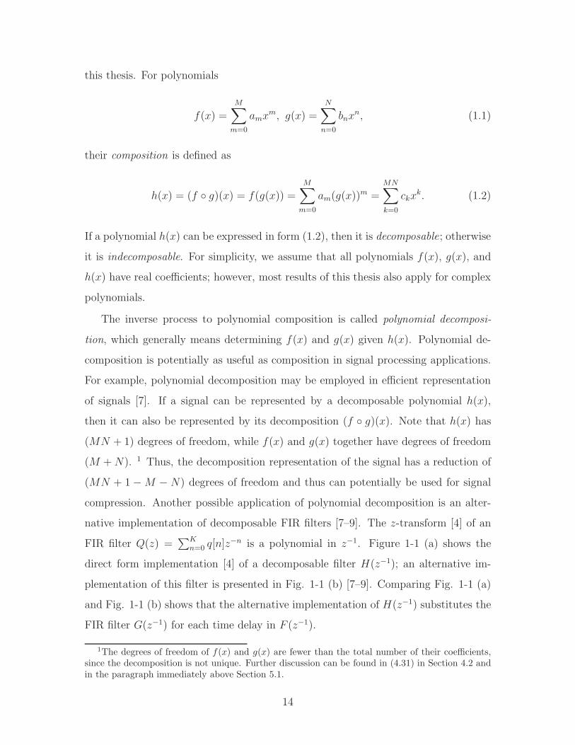
native implementation of decomposable FIR filters [7–9]. The z-transform [4] of an
FIR filter Q(z) =∑K
n=0 q[n]z−n is a polynomial in z−1. Figure 1-1 (a) shows the
direct form implementation [4] of a decomposable filter H(z−1); an alternative im-
plementation of this filter is presented in Fig. 1-1 (b) [7–9]. Comparing Fig. 1-1 (a)
and Fig. 1-1 (b) shows that the alternative implementation of H(z−1) substitutes the
FIR filter G(z−1) for each time delay in F (z−1).
1The degrees of freedom of f(x) and g(x) are fewer than the total number of their coefficients,since the decomposition is not unique. Further discussion can be found in (4.31) in Section 4.2 andin the paragraph immediately above Section 5.1.
14

Another related problem is approximate decomposition, which determines f(x)
and g(x) such that h(x) ≈ (f ◦ g)(x) for an indecomposable polynomial h(x). Ap-
proximate decomposition may have wider applications than exact decomposition,
since most real signals are unlikely to be exactly decomposable. The above argument
about reduction in degrees of freedom implies the low density of decomposable poly-
nomials in the polynomial space. In particular, givenM and N , all the decomposable
polynomials are located on a manifold of dimensions (M +N), while the whole space
has (MN + 1) dimensions. As the length (MN + 1) of the polynomial increases, the
reduction in degrees of freedom also grows, which makes decomposable polynomials
less and less dense in the polynomial space. Thus, it is unlikely that an arbitrarily
long signal will correspond to an exactly decomposable polynomial.
Indecomposable polynomials can possibly be represented by approximate decom-
position. For example, if a signal corresponds to an indecomposable polynomial h(x),
the approximate decomposition method might be employed in compressing the sig-
nal into the composition of f(x) and g(x), with a decrease in degrees of freedom by
(MN +1−M −N) and possibly without much loss in quality. However, since exact
decomposition can be thought of as a problem of identification while approximate
decomposition corresponds to modeling, approximate decomposition appears much
more challenging than exact decomposition.
1.2 Objective
Many of the applications of functional composition are currently being explored by
Sefa Demirtas [7]. The primary goals of this thesis are to theoretically evaluate the ro-
bustness of polynomial composition and decomposition as well as to develop effective
algorithms for the decomposition problems in both the exact and the approximate
cases. 2
Robustness is characterized by sensitivities of composition and decomposition,
2Many of the results in this thesis are included in [10, 11] by S. Demirtas, G. Su, and A. V.Oppenheim.
15

z−1 z−1 z−1· · ·
· · ·
c0 c1 c2 cMN−1 cMN
x[n]
y[n]m m m m- - - - - -
- - - -
? ? ? ?
(a) Direct Form [4]
G(z−1) G(z−1) G(z−1)· · ·
· · ·
a0 a1 a2 aM−1 aM
x[n]
y[n]m m m m- - - - - -
- - - -
? ? ? ?
(b) Alternative Implementation [7–9]
Figure 1-1: Two Implementations of a Decomposable FIR Filter where H(z−1) =(F ◦G)(z−1)
where the sensitivities represent the maximum relative magnification of the energy
among all small perturbations. Lower sensitivity indicates higher robustness and
higher reliability in applications. Equivalent compositions are shown to be effective
to decrease certain sensitivities, especially when the degree of h(x) is high.
New algorithms are proposed for both the exact and the approximate decom-
position problems. We propose two types of decomposition algorithms: those with
polynomial coefficients as input and those with polynomial roots as input. Differ-
ent algorithms have different capabilities to decompose high order polynomials and
different robustness to noise.
The remainder of this thesis is organized as follows. Chapter 2 briefly summarizes
the basic properties and existing work on polynomial decomposition. Chapter 3
states the precise definition of the problems that will be explored in this thesis. The
sensitivities are theoretically studied in Chapter 4, where we also develop an approach
to decrease certain sensitivities by equivalent compositions. The algorithms for the
exact and the approximate decomposition problems are presented and evaluated with
numerical simulation in Chapter 5 and 6, respectively. Chapter 7 concludes this thesis
and proposes potential problems for future work.
16
Chapter 2
Background
2.1 Polynomial Composition Properties
A number of basic properties that will be utilized about polynomial composition are
briefly stated in this section. The proofs of these properties are omitted and can be
found in the references [12, 13].
1. Polynomial composition is linear with respect to f(x) but not to g(x). Namely,
(f1 + f2) ◦ g = f1 ◦ g + f2 ◦ g always holds, but generally f ◦ (g1 + g2) 6=
(f ◦ g1) + (f ◦ g2).
2. Polynomial composition satisfies the associative law, i.e., (f ◦g)◦p = f ◦ (g ◦p).
3. Polynomial composition generally does not satisfy the commutative law, i.e.,
(f ◦g) 6= (g ◦f) in general. However, two special situations are worthy of notice
[12]. The cyclic polynomials, which have only a single power term xn, satisfy
xMN = xM ◦xN = xN ◦xM . Similarly, TMN (x) = (TM ◦TN)(x) = (TN ◦TM)(x),
where Tn(x) = cos(n arccos(x)) is the nth-order Chebyshev Polynomial.
4. Polynomial composition is not unique in the following three situations. First, it
holds in general that f ◦ g = (f ◦ q−1) ◦ (q ◦ g), where q(x) = q1x+ q0 is a first-
degree polynomial and q−1(x) = (x−q0)/q1 is the inverse function of q(x) under
composition. Second, xMN(v(xM)
)M= xM ◦
(xNv(xM)
)=(xN(v(x))M
)◦ xM
17

where v(x) is an arbitrary polynomial. Third, as stated above, the Chebyshev
polynomials can have more than one decomposition. These three scenarios of
non-unique decomposition include all possible situations: if there are two ways
to decompose a given polynomial into indecomposable components, then the
two ways of decomposition can differ only in the above three situations, as is
described more precisely in [13] on this topic.
5. If h(x) is decomposable, the flipped polynomial hflip(x) =∑MN
k=0 cMN−kxk is
not necessarily decomposable.
6. Similar to a minimum phase filter [4], we refer to h(x) as a minimum phase
polynomial if all the roots are inside the unit circle. If f(x) and g(x) are both
minimum phase, the composition h(x) is not necessarily minimum phase. How-
ever, as is shown in Appendix A, if a decomposable polynomial h(x) is minimum
phase, then there always exists a non-trivial minimum phase decomposition.
More precisely, if a minimum phase polynomial h(x) is decomposable into two
components with degrees M and N (M > 1 and N > 1), then we can construc-
t an equivalent composition of h(x), the components in which have the same
degrees and are both minimum phase polynomials. The proof in Appendix A
also provides the construction of a minimum phase decomposition from a non-
minimum phase decomposition of a minimum phase decomposable polynomial,
which may have potential application in implementation of minimum phase
decomposable filters.
7. Similar to a linear phase filter [4], we refer to h(x) as a linear phase polynomial
if the coefficients have odd or even symmetry. If f(x) and g(x) are both linear
phase, the composition h(x) is not necessarily linear phase. If a decomposable
h(x) is linear phase, there may not exist a non-trivial decomposition with linear
phase components, where non-trivial means the degrees of the components are
both larger than one.
18
2.2 Review of Existing Polynomial Decomposition
Algorithms
This section briefly summarizes the existing polynomial decomposition algorithms.1
In mathematics and symbolic algebraic computation, polynomial decomposition has
been an important topic for decades [14–24]. The first algorithm for the exact de-
composition problem was proposed by Barton and Zippel in [14]. This algorithm is
based on deep mathematical results to convert the univariate polynomial decompo-
sition problem into the bivariate polynomial factorization problem [15, 19] and has
exponential-time complexity. Recently, Barton’s algorithm has been improved to
polynomial-time complexity in [16], and extended into the approximate decomposi-
tion problem [16]. An alternative decomposition algorithm was proposed by Kozen
and Landau in [17], which requires the degreesM andN of f(x) and g(x), respectively.
Compared with Barton’s method, Kozen’s algorithm is much more straightforward
to implement. A third type of algorithm was based on the algorithm that Aubry
and Valibouze described in [20], which explores the relationship between the coeffi-
cients and the roots of a polynomial. Kozen’s algorithm is theoretically equivalent
to Aubry’s algorithm; however, they may show significantly different robustness in
numerical computation.
Approximate decomposition algorithms fall into two main categories. The first
category is to find a locally optimal solution based on the assumption that the input
polynomial h(x) is the sum of a decomposable polynomial and a small perturba-
tion. The algorithm proposed by Corless et al. in [18] belongs to this category; this
algorithm employs the result in [17] as an initial value and proceeds iteratively to
find a locally optimal approximate solution. However, the assumption that h(x) is
a nearly decomposable polynomial would not hold in most cases, and this fact in
general constrains the applicability of Corless’s algorithm. Moreover, there is no gen-
eral guarantee for the convergence of this algorithm, nor the global optimality of the
result.
1Much of this background was uncovered by Sefa Demirtas [11].
19
The second category of approximate decomposition algorithms is a generalization
of Barton’s algorithm [14] that employs bivariate polynomial factorization [15, 19].
This approach has a deep theoretical foundation and makes no assumption that h(x)
is nearly decomposable. As an example, Giesbrecht and May [16] employ the theo-
retical results in [19, 25] and convert the approximate decomposition problem into a
special case of the Structured Total Least Squares (STLS) problem [21,24]. There are
a number of heuristic algorithms to solve the STLS problem, such as the Riemanni-
an Singular Value Decomposition (RiSVD) algorithm [21] and the weighted penalty
relaxation algorithm [22,26]. However, none of these heuristic algorithms guarantees
convergence or global optimality in a general setting, which may be a disadvantage of
this type of approach. The Ruppert matrix [25], which is critical in the corresponding
STLS problem, has such high dimension that the numerical accuracy and efficiency
may become problematic. In summary, determining the optimal approximate decom-
position of an arbitrary polynomial still remains a challenging problem.
Theoretically, it does not appear to be possible to determine the distance from
the given h(x) to the nearest decomposable polynomial. Although there is a lower
bound on this distance in [16], this bound may not be sufficiently tight.
20

Chapter 3
Problem Definition
In this chapter, we state the problems to be explored in this thesis. The goal of
this thesis is to theoretically study the robustness of polynomial composition and
decomposition, and to design polynomial decomposition algorithms for both the exact
and the approximate cases.1 The robustness is characterized by the sensitivities in
Section 3.1. For both the exact decomposition in Section 3.2 and the approximate
decomposition in Section 3.3, there are two problems defined with different input
information.
3.1 Sensitivity Analysis
In polynomial composition, a perturbation of the components will typically result in a
corresponding perturbation of the composed polynomial, and vice versa for polynomi-
al decomposition. For example, if the component f(x) has a perturbation of ∆f(x),
then there is a corresponding perturbation ∆h(x) = ((f + ∆f) ◦ g)(x) − (f ◦ g)(x)
in the composed polynomial h(x) = (f ◦ g)(x). However, the energy of perturbation
can be significantly different between the components and the composed polynomial.
Sensitivities for the composition operation describe the maximal extent to which the
small perturbation of the polynomial components is magnified in the perturbation
of the composed polynomial [10], and sensitivities for the decomposition operation
1Many of the results were developed in collaboration with Sefa Demirtas [7].
21

describe the inverse maximum magnification.
3.1.1 Sensitivities of the Coefficients
In this section, we consider the sensitivities of the coefficients of the polynomials. In
the composition h(x) = (f ◦ g)(x), the sensitivity from f(x) to h(x) is defined as [10]
Sf→h = max‖∆f‖2=κ
(R∆h
R∆f
), (3.1)
where R∆h and R∆f are defined as
R∆h =‖∆h‖22‖h‖22
, and R∆f =‖∆f‖22‖f‖22
, (3.2)
in which f , h, ∆f , and ∆h are vectors of the coefficients of respective polynomials,
‖ · ‖2 denotes the l2-norm, and κ is the magnitude of the perturbation ∆f which
is constrained to be sufficiently small. To a first-order approximation, Sf→h and
other sensitivities become independent of the specific value of κ when κ is sufficiently
small. Both R∆h and R∆f are the ratios of the perturbation polynomial energy over
the original polynomial energy, and they represent the relative perturbation of h(x)
and f(x), respectively. If we consider the coefficients of polynomials as vectors, then
the sensitivity Sf→h is the maximum magnification of the relative perturbation from
f(x) to h(x), among all possible directions of perturbation. Since the sensitivity is
defined in the worst case scenario, it serves as an upper bound on the ratio between
relative perturbation R∆h
R∆fwhen the perturbation ∆f is small.
Similarly, we can define the sensitivity from g(x) to h(x) in the composition process
[10],
Sg→h = max‖∆g‖2=κ
(R∆h
R∆g
), (3.3)
where R∆h is defined in (3.2) and R∆g denotes
R∆g =‖∆g‖22‖g‖22
, (3.4)
22

in which the magnitude κ of the perturbation∆g is sufficiently small. This sensitivity
involves the worst direction of the perturbation of g(x), in which the perturbation is
maximally magnified after composition.
In the composition process, the resulting polynomial is of course decomposable
even after perturbation of its components. In contrast, a decomposable polynomial
can become indecomposable after an arbitrary perturbation. Consequently, compo-
nents do not exist for the perturbed polynomial, and thus sensitivities are undefined
in this scenario. In addition, even if the polynomial remains decomposable after per-
turbation, the degrees of the components may change, which again makes it difficult
to assess the sensitivities. To avoid these situations, in our discussion of sensitivities
in the decomposition operation, we consider only the perturbation after which the
polynomial still remains decomposable and the degrees of the components remain the
same. In such cases, the sensitivities of the decomposition process imply the extent
to which an error is magnified from the composed polynomial to its components.
With the constraints specified above on the perturbation, the sensitivity from h(x)
to f(x) is defined as [10]
Sh→f = max‖∆f‖2=κ
(R∆f
R∆h
), (3.5)
and the sensitivity from h(x) to g(x) is defined as [10]
Sh→g = max‖∆g‖2=κ
(R∆g
R∆h
), (3.6)
where perturbations ∆f and ∆g have sufficiently a small magnitude of κ.
In summary, the sensitivities within the coefficient triplet (f, g, h) are defined in
Table 3.1.
3.1.2 Sensitivities of the Roots
Before we introduce the sensitivities of the roots, we first show the relationship of
roots of the polynomials in the composition process. Denoting zh as a root of h(x),
23

Table 3.1: Definitions of the Sensitivities within the Coefficient Triplet (f, g, h)From To Process Sensitivity Definition
f h Composition Sf→h = max‖∆f‖2=κ
(R∆h
R∆f
)
g h Composition Sg→h = max‖∆g‖2=κ
(R∆h
R∆g
)
h f Decomposition Sh→f = max‖∆f‖2=κ
(R∆f
R∆h
)
h g Decomposition Sh→g = max‖∆g‖2=κ
(R∆g
R∆h
)
then h(zh) = f(g(zh)) = 0. Thus, if we define
zf , g(zh), (3.7)
then f(zf) = 0 and zf is a root of f(x). In other words, evaluating the polynomial
g(x) at the roots of h(x) results in the roots of f(x); equivalently, the roots zh
of the composed polynomial are the solutions to the equation (3.7) when zf and
g(x) are both determined. As a result, the root relationship (3.7) can be regarded
as a description of polynomial composition that is alternative to (1.2): while (1.2)
characterizes the relationship among the coefficients f , g, and h in the composition
process, (3.7) describes the relationship among zf , g, and zh.
We can also study the robustness of polynomial composition and decomposition
from the perspective of the relationship among the root triplet (zf , g, zh) in (3.7).
If zf or g(x) are perturbed, then there will typically be a corresponding perturba-
tion in zh to satisfy the constraint (3.7); similarly, perturbation in zh will typically
result in perturbations in zf and g(x), under the assumption of decomposability of
the perturbed polynomial into components with unchanged degrees. As a result,
the worst-case magnification of the magnitude of perturbation can be described by
sensitivities.
In Section 3.1.1, we have shown sensitivities that are described within the coef-
ficient triplet (f, g, h) and listed in Table 3.1; similarly, we can define four new
sensitivities within the root triplet (zf , g, zh). The four new sensitivities are summa-
24
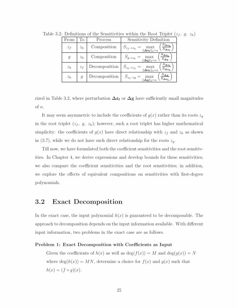
Table 3.2: Definitions of the Sensitivities within the Root Triplet (zf , g, zh)From To Process Sensitivity Definition
zf zh Composition Szf→zh = max‖∆zf‖2=κ
(R∆zh
R∆zf
)
g zh Composition Sg→zh = max‖∆g‖2=κ
(R∆zh
R∆g
)
zh zf Decomposition Szh→zf = max‖∆zf‖2=κ
(R∆zf
R∆zh
)
zh g Decomposition Szh→g = max‖∆g‖2=κ
(R∆g
R∆zh
)
rized in Table 3.2, where perturbation ∆zf or ∆g have sufficiently small magnitudes
of κ.
It may seem asymmetric to include the coefficients of g(x) rather than its roots zg
in the root triplet (zf , g, zh); however, such a root triplet has higher mathematical
simplicity: the coefficients of g(x) have direct relationship with zf and zh as shown
in (3.7), while we do not have such direct relationship for the roots zg.
Till now, we have formulated both the coefficient sensitivities and the root sensitiv-
ities. In Chapter 4, we derive expressions and develop bounds for these sensitivities;
we also compare the coefficient sensitivities and the root sensitivities; in addition,
we explore the effects of equivalent compositions on sensitivities with first-degree
polynomials.
3.2 Exact Decomposition
In the exact case, the input polynomial h(x) is guaranteed to be decomposable. The
approach to decomposition depends on the input information available. With different
input information, two problems in the exact case are as follows.
Problem 1: Exact Decomposition with Coefficients as Input
Given the coefficients of h(x) as well as deg(f(x)) =M and deg(g(x)) = N
where deg(h(x)) =MN , determine a choice for f(x) and g(x) such that
h(x) = (f ◦ g)(x).
25

Problem 2: Exact Decomposition with Roots as Input
Given the roots of h(x) as well as deg(f(x)) =M and deg(g(x)) = N
where deg(h(x)) =MN , determine a choice for f(x) and g(x) such that
h(x) = (f ◦ g)(x).
The above two problems are of course closely related. On the one hand, they are
theoretically equivalent, since the coefficients of a polynomial determine the roots,
and vice versa. On the other hand, the two problems have considerable differences
in numerical computation. Obtaining the roots from the coefficients is difficult for a
polynomial whose degree is high or whose roots are clustered. Thus, an algorithm
for Problem 1 may have better performance than an algorithm that first determines
the roots from the coefficients and then solves Problem 2, since the roots may be
numerically inaccurate. For similar reasons, an algorithm that directly works with
roots may be more robust than an algorithm that first obtains the coefficients and
then solves Problem 1. In fact, algorithms with polynomial coefficients as input and
those with roots as input may have considerably different performance.
The solutions to both problems are potentially useful in signal processing. If we
want to decompose a decomposable signal, the signal values naturally correspond to
the coefficients of the z-transform, which is in the form of Problem 1. In addition
to the coefficients, the roots of polynomials are also important in the z-transform
of a filter and the pole-zero analysis of the transfer function of a system. With the
knowledge of precise roots in such applications, Problem 2 is potentially useful.
In the statements of both problems, the degrees of components are included in the
input information. However, we can also perform decomposition for a decomposable
polynomial without knowing the degrees of the components. Since the product of
the degrees of the components equals to the degree of the composed polynomial,
we can perform the decomposition algorithms for each candidate pair of degrees of
the components, and then we check whether the output of the algorithms is a valid
decomposition. In this case, the computational complexity is higher than the scenario
where the degrees of components are available.
26
3.3 Approximate Decomposition
In this class of problems, we consider indecomposable polynomials; i. e. h(x) 6= (f ◦
g)(x) for any non-trivial f(x) and g(x). In this case, our goal is to find a decomposable
polynomial nearest in some sense to h(x) as the approximate decomposition. The
problems are defined with a one-to-one correspondence to those in the exact case.
Problem 3: Approximate Decomposition with Coefficients as Input
Given the coefficients of h(x) as well as deg(f(x)) =M and deg(g(x)) = N
where deg(h(x)) =MN , determine a choice for f(x) and g(x) minimizing
dist(h(x), (f ◦ g)(x)).
Problem 4: Approximate Decomposition with Roots as Input
Given the roots of h(x) as well as deg(f(x)) =M and deg(g(x)) = N
where deg(h(x)) =MN , determine a choice for f(x) and g(x) minimizing
dist(h(x), (f ◦ g)(x)).
Here dist(s(x), t(x)) is a distance measure between polynomials s(x) and t(x) with
the same degree. As an example, [18] uses the l2 norm corresponding to the energy
of the residue error:
‖s(x)− t(x)‖2 =
(P∑
k=0
|sk − tk|2
) 12
, (3.8)
where P = deg(s(x)) = deg(t(x)).
Similar to the exact case, these two problems here are also related. Although the
two problems are equivalent in theory, the algorithms for the two problems may have
different numerical performance.
27

28

Chapter 4
Sensitivities of Polynomial
Composition and Decomposition
This chapter explores the sensitivities of polynomial composition and decomposition
to study their robustness, as proposed in Section 3.1. 1 Derivation and bounds for the
sensitivities are developed in Section 4.1. The effects of equivalent compositions with
first-degree polynomials on sensitivities are studied in Section 4.2, with the proposal
of a rule for parameter selection to approach the minimum sensitivities. Simulation
results are shown in Section 4.3.
4.1 Derivation of the Sensitivities
4.1.1 Sensitivities of the Coefficients
In this section, we derive the expressions and bounds for Sf→h, Sg→h, Sh→f , and Sh→g
that are defined in Table 3.1. First, we derive the sensitivities of f(x) and h(x) with
respect to each other. The polynomial composition h(x) = (f ◦ g)(x) in (1.2) can be
equivalently presented by the following linear equations:
h = Gf , (4.1)
1Many of the results in this chapter are summarized in [10] by S. Demirtas, G. Su, and A. V.Oppenheim.
29

where the vectors f = [aM , aM−1, . . . , a0]T and h = [cMN , cMN−1, . . . , c0]
T have el-
ements as the coefficients of respective polynomials, and the matrix G is the self-
convolution matrix of the polynomial g(x)
G = [gM , . . . , g2, g1, g0]. (4.2)
From (4.1), it follows that the perturbations satisfy the linear relationship
∆h = G∆f . (4.3)
Thus, the maximal magnification of perturbation energy between ∆f(x) and ∆h(x)
is
Sf→h = max‖∆f‖2=κ
(R∆h
R∆f
)=
‖f‖22‖h‖22
· max‖∆f‖2=κ
(‖G∆f‖22‖∆f‖22
)= σ2
G,max
‖f‖22‖h‖22
, (4.4)
where σG,max is the largest singular value of the matrixG. If the perturbation∆f is in
the direction of the maximal magnification of the matrixG, then the sensitivity above
is achieved. In addition, the sensitivity in (4.4) does not depend on the magnitude κ
of the perturbation, due to the linear relationship in (4.3).
For a fixed polynomial g(x), we can obtain an upper bound for the sensitivity
Sf→h over all possible polynomials f(x) with degree M . Since h = Gf ,
σ2G,min ≤
‖h‖22‖f‖22
≤ σ2G,max,
where σG,min is the smallest singular value of the matrix G. Consequently, the sensi-
tivity Sf→h is bounded by
1 ≤ Sf→h ≤ cond(G)2, (4.5)
where cond(G) =σG,max
σG,minis the condition number of the matrix G. The upper bound
in (4.5) depends only on the polynomial g(x) and the degree of f(x), since the matrix
G is the self-convolution matrix of g(x) up to the power of M . The upper and lower
bounds in (4.5) are both tight in theory; however, the sensitivity with a given f(x)
30
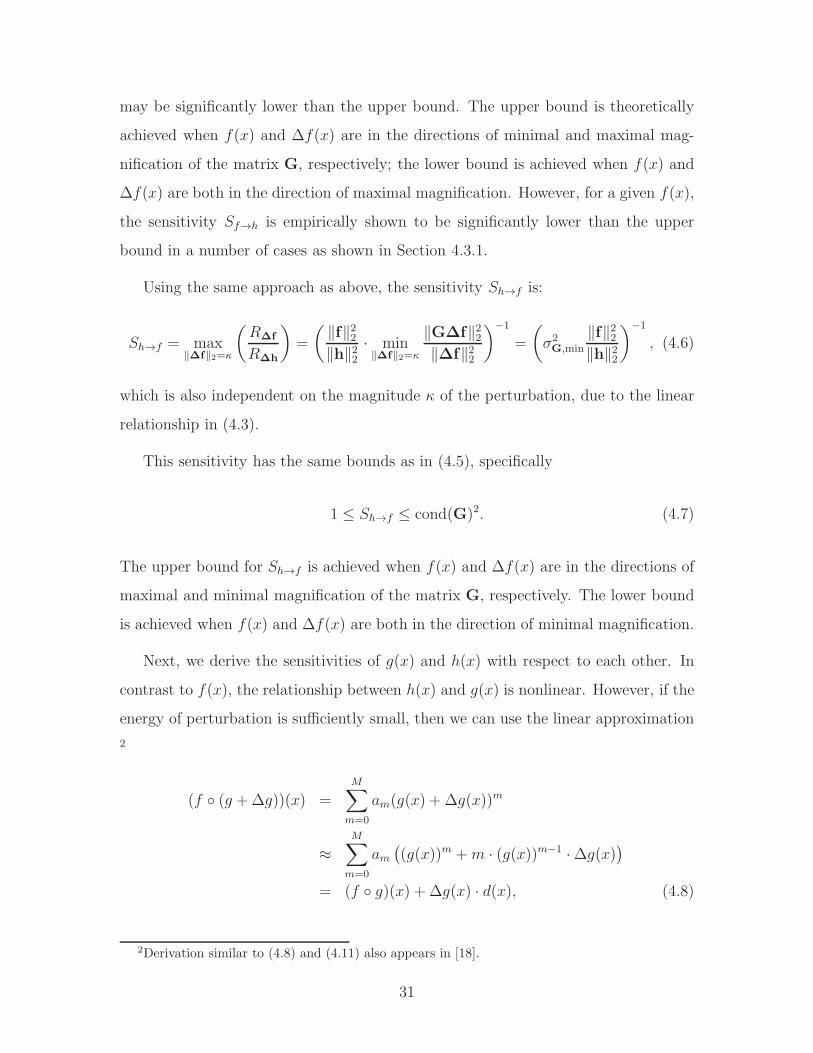
may be significantly lower than the upper bound. The upper bound is theoretically
achieved when f(x) and ∆f(x) are in the directions of minimal and maximal mag-
nification of the matrix G, respectively; the lower bound is achieved when f(x) and
∆f(x) are both in the direction of maximal magnification. However, for a given f(x),
the sensitivity Sf→h is empirically shown to be significantly lower than the upper
bound in a number of cases as shown in Section 4.3.1.
Using the same approach as above, the sensitivity Sh→f is:
Sh→f = max‖∆f‖2=κ
(R∆f
R∆h
)=
(‖f‖22‖h‖22
· min‖∆f‖2=κ
‖G∆f‖22‖∆f‖22
)−1
=
(σ2G,min
‖f‖22‖h‖22
)−1
, (4.6)
which is also independent on the magnitude κ of the perturbation, due to the linear
relationship in (4.3).
This sensitivity has the same bounds as in (4.5), specifically
1 ≤ Sh→f ≤ cond(G)2. (4.7)
The upper bound for Sh→f is achieved when f(x) and ∆f(x) are in the directions of
maximal and minimal magnification of the matrix G, respectively. The lower bound
is achieved when f(x) and ∆f(x) are both in the direction of minimal magnification.
Next, we derive the sensitivities of g(x) and h(x) with respect to each other. In
contrast to f(x), the relationship between h(x) and g(x) is nonlinear. However, if the
energy of perturbation is sufficiently small, then we can use the linear approximation
2
(f ◦ (g +∆g))(x) =
M∑
m=0
am(g(x) + ∆g(x))m
≈
M∑
m=0
am((g(x))m +m · (g(x))m−1 ·∆g(x)
)
= (f ◦ g)(x) + ∆g(x) · d(x), (4.8)
2Derivation similar to (4.8) and (4.11) also appears in [18].
31

where d(x) is the composition of f ′(x) (the derivative of f(x)) and g(x):
d(x) =
(M−1)N∑
k=0
dkxk = (f ′ ◦ g)(x). (4.9)
Consequently, we have
∆h(x) = (f ◦ (g +∆g))(x)− (f ◦ g)(x) ≈ ∆g(x) · d(x), (4.10)
which indicates that ∆h(x) is approximately the convolution of ∆g(x) and d(x), when
∆g(x) is sufficiently small. Expressed in matrix form,
∆h ≈ D∆g, (4.11)
where the matrix D is a (MN +1)× (N +1) Teoplitz matrix with the last column as
[0, 0, . . . , 0, d(M−1)N , d(M−1)N−1, . . . , d0]T. Consequently, the sensitivity Sg→h defined
in (3.3) becomes
Sg→h =‖g‖22‖h‖22
· max‖∆g‖2=κ
(‖∆h‖22‖∆g‖22
)
=‖g‖22‖h‖22
· max‖∆g‖2=κ
(‖D∆g‖22‖∆g‖22
)
= σ2D,max ·
‖g‖22‖h‖22
, (4.12)
where σD,max is the maximum singular value of the matrix D, and the perturbation
∆g has a sufficiently small magnitude of κ.
As developed in Appendix B, the sensitivity Sg→h has the upper bound
Sg→h ≤ (N + 1)‖g‖22 · σ2T,max, (4.13)
where σT,max is the maximum singular value of the matrix T:
T = GV(GTG)−1GT. (4.14)
32

The matrix V in (4.14) is a (M + 1) × (M + 1) matrix with sub-diagonal elements
M,M − 1,M − 2, . . . , 2, 1 and other elements as zero, i.e.,
V =
0
M 0
M−1 0
0
. . .
00
2 0
1 0
. (4.15)
This upper bound holds for all possible polynomials f(x) with a fixed degree
M and a fixed polynomial g(x). Although this bound is not always tight for any
g(x), numerical simulations presented in Section 4.3.1 indicate empirically that it is
a reasonably good estimate.
The sensitivity Sh→g in the decomposition process can be derived in an approach
similar to that used for Sg→h:
Sh→g = max‖∆g‖2=κ
(R∆g
R∆h
)
=
(‖g‖22‖h‖22
· min‖∆g‖2=κ
(‖∆h‖22‖∆g‖22
))−1
=
(‖g‖22‖h‖22
· min‖∆g‖2=κ
(‖D∆g‖22‖∆g‖22
))−1
=
(σ2D,min ·
‖g‖22‖h‖22
)−1
, (4.16)
where σD,min is the minimum singular value of the matrix D, and the perturbation
∆g has a sufficiently small magnitude of κ.
4.1.2 Sensitivities of the Roots
In this section, we analyze the sensitivities among the triplet (zf , g , zh), which are
defined in Table 3.2. Before the derivation of the sensitivities, we study the structure
33

of the roots of decomposable polynomials.
If we denote the roots of f(x) and h(x) as zf(i) (1 ≤ i ≤ M) and zh(k) (1 ≤
k ≤ MN), respectively, then the composed polynomial h(x) can be factored in the
following two ways:
h(x) = aM
M∏
i=1
(g(x)− zf (i)) = cMN
MN∏
k=1
(x− zh(k)) , (4.17)
where aM and cMN are the coefficients of the highest degree term in f(x) and h(x),
respectively. If we denote
gi(x) = g(x)− zf(i), 1 ≤ i ≤ M, (4.18)
then (4.17) shows that the union of the roots of all gi(x) forms the roots of h(x). Thus,
we can partition the roots zh(k) (1 ≤ k ≤ MN) into M groups Ai (1 ≤ i ≤ M),
where all the roots in the i-th group Ai satisfy gi(x) = 0, i.e.,
Ai = {k | g(zh(k)) = zf (i), 1 ≤ k ≤ MN} , 1 ≤ i ≤M. (4.19)
There are N elements in each group Ai; the roots in a group correspond to the same
one root of f(x).
To simplify the analysis of the sensitivity of the roots, we assume that the deriva-
tive of g(x) is non-zero at the roots of h(x), i.e., g′(zh(i)) 6= 0 for 1 ≤ i ≤ MN . In
fact, this assumption holds in most scenarios: if h(x) has only single roots, then it
ensures g′(zh) 6= 0, since h′(zh) 6= 0 and h′(x) = f ′(g(x))g′(x).
First, we consider the sensitivities of zf and zh with respect to each other, when
the polynomial g(x) is fixed. Since the roots zh in each group correspond to the
same root of f(x), the perturbation of zf (i) affects only those roots of h(x) that
correspond to zf (i), i.e., zh(k) where k ∈ Ai. For a sufficiently small perturbation
∆zh(k) (k ∈ Ai), we can employ the following linear approximation
g (zh(k) + ∆zh(k)) ≈ g(zh(k)) + g′(zh(k)) ·∆zh(k), k ∈ Ai,
34

so the the perturbation ∆zf (i) is
∆zf (i) = g (zh(k) + ∆zh(k))− g(zh(k)) ≈ g′(zh(k)) ·∆zh(k), k ∈ Ai.
Consequently, if we perturb only one root zf (i), the ratio of perturbation energy is
‖∆zh‖22
‖∆zf‖22
=
∑k∈Ai
|∆zh(k)|2
|∆zf(i)|2≈∑
k∈Ai
1
|g′(zh(k))|2. (4.20)
With the assumption that g′(zh) 6= 0, the ratio in (4.20) is finite.
If two or more roots of f(x) are perturbed, then each zf (i) affects the corre-
sponding roots of h(x) (i.e., zh(k), k ∈ Ai) independently. In this case, the ratio of
perturbation energy is
‖∆zh‖22
‖∆zf‖22
=
∑Mi=1
(∑k∈Ai
|∆zh(k)|2)
∑Mi=1 |∆zf (i)|
2≈
∑M
i=1 |∆zf (i)|2(∑
k∈Ai
1|g′(zh(k))|2
)
∑Mi=1 |∆zf(i)|
2. (4.21)
Since (4.21) is a weighted summation of (4.20) over the range of i = 1, 2, . . . ,M , we
know
mini∈{1,2,...,M}
∑
k∈Ai
1
|g′(zh(k))|2≤
‖∆zh‖22
‖∆zf‖22
≤ maxi∈{1,2,...,M}
∑
k∈Ai
1
|g′(zh(k))|2,
Consequently, the sensitivity Szf→zh in the composition process can be derived:
Szf→zh = max‖∆zf‖2=κ
R∆zh
R∆zf
=‖zf‖
22
‖zh‖22
· max‖∆zf‖2=κ
‖∆zh‖22
‖∆zf‖22
=‖zf‖
22
‖zh‖22
·
(max
i∈{1,2,...,M}
∑
k∈Ai
1
|g′(zh(k))|2
), (4.22)
35

and the sensitivity Szh→zf in the decomposition process is:
Szh→zf = max‖∆zf‖2=κ
R∆zf
R∆zh
=
(min
‖∆zf‖2=κ
R∆zh
R∆zf
)−1
=
(‖zf‖
22
‖zh‖22·
(min
i∈{1,2,...,M}
∑
k∈Ai
1
|g′(zh(k))|2
))−1
, (4.23)
where the perturbation ∆zf has a sufficiently small magnitude of κ.
It is shown in (4.22) and (4.23) that the sensitivities depend on the derivative of
g(x) at the roots of h(x). This dependence is intuitive from the fact that zf = g(zh):
if the derivatives g′(zh) have small magnitudes, then a big perturbation on zh may
still result in a small perturbation on zf , so the composition sensitivity Szf→zh may
be large while the decomposition sensitivity Szh→zf may be small; in contrast, a
large derivative could result in a small composition sensitivity Szf→zh and a large
decomposition sensitivity Szh→zf .
As a result, the clustered roots of h(x) influence the robustness between zf and
zh in composition and decomposition. For composition, if h(x) has clustered roots in
one group Ai, then the derivatives g′(zh) at those clustered roots have small values,
so the composition operation is vulnerable to noise. In contrast, if h(x) does not have
clustered roots, or the clustered roots belong to different groups, then the composition
operation is robust. For decomposition, if clustered roots appear in each group Ai,
then the sensitivity Szh→zf has a low value, so the decomposition has high robustness.
Next we derive the sensitivities of zh and g(x) with respect to each other, i.e., Sg→zh
in the composition process and Szh→g in the decomposition process. In contrast to
the sensitivities between zh and zf where changing one root zf affects only N roots
of h(x), a perturbation of g(x) results in perturbation of all roots of h(x). When the
roots of f(x) are all fixed, we have the following relationship between perturbations
of g(x) and the roots of h(x):
g(zh(k) + ∆zh(k)) + ∆g(zh(k) + ∆zh(k)) = zf (i), k ∈ Ai.
36

Applying linear approximation with small perturbations,
g(zh(k) + ∆zh(k)) ≈ zf (i) + g′(zh(k)) ·∆zh(k),
∆g(zh(k) + ∆zh(k)) ≈ ∆g(zh(k)),
the perturbation of zh(k) is derived as
∆zh(k) ≈ −∆g(zh(k))
g′(zh(k)).
The perturbations of all roots of h(x) can be expressed in matrix form as:
∆zh ≈ −QW∆g (4.24)
where matrices Q and W are
Q = diag
(1
g′(zh(1)),
1
g′(zh(2)), . . . ,
1
g′(zh(MN))
), (4.25)
W =
zNh (1) zN−1h (1) · · · zh(1) 1
zNh (2) zN−1h (2) · · · zh(2) 1
......
. . ....
...
zNh (MN) zN−1h (MN) · · · zh(MN) 1
. (4.26)
Consequently, we can derive the sensitivities Sg→zh in the composition process and
Szh→g in the decomposition process:
Sg→zh = max‖∆g‖2=κ
(R∆zh
R∆g
)= σ2
QW,max
‖g‖22‖zh‖22
, (4.27)
Szh→g = max‖∆g‖2=κ
(R∆g
R∆zh
)=
(σ2QW,min
‖g‖22‖zh‖22
)−1
, (4.28)
where σQW,max and σQW,min are the maximum and minimum singular values of the
matrix Q ·W, respectively; the perturbation ∆g has a sufficiently small magnitude
of κ.
37

4.2 Sensitivities of Equivalent Compositions with
First-Degree Polynomials
As mentioned in Section 2.1, a composed polynomial may have equivalent composi-
tions when first-degree polynomials are used. Specifically, if we denote
f(x) =(f ◦ q−1
)(x), (4.29)
g(x) = (q ◦ g) (x), (4.30)
where q(x) = q1x+ q0 is a first-degree polynomial, then we have
h(x) = (f ◦ g)(x) =(f ◦ g
)(x). (4.31)
However, these equivalent compositions may have different sensitivities. In this sec-
tion, we show the effects of equivalent compositions on sensitivities, and we propose
a practical rule to choose the parameters of the first-degree polynomial to get to a
point that is near the minimum of certain sensitivities.
First, we analyze the sensitivities between the coefficients of f(x) and h(x). Ap-
plying (4.1) to the equivalent composition (4.31), we have
h = Gf , (4.32)
where the matrix G has columns as the self-convolutions of the new polynomial g(x).
The self-convolution (g(x))n can be regarded as a composition
(g(x))n = (q1g(x) + q0)n = (sn ◦ g) (x), (4.33)
where the polynomial sn(x) = (q1x+ q0)n. Connecting (4.33) with the matrix formu-
lation in (4.1), we have
[(g(x))n] = Gsn,
where [(g(x))n] is the corresponding vector of the polynomial (g(x))n. As a result, we
38
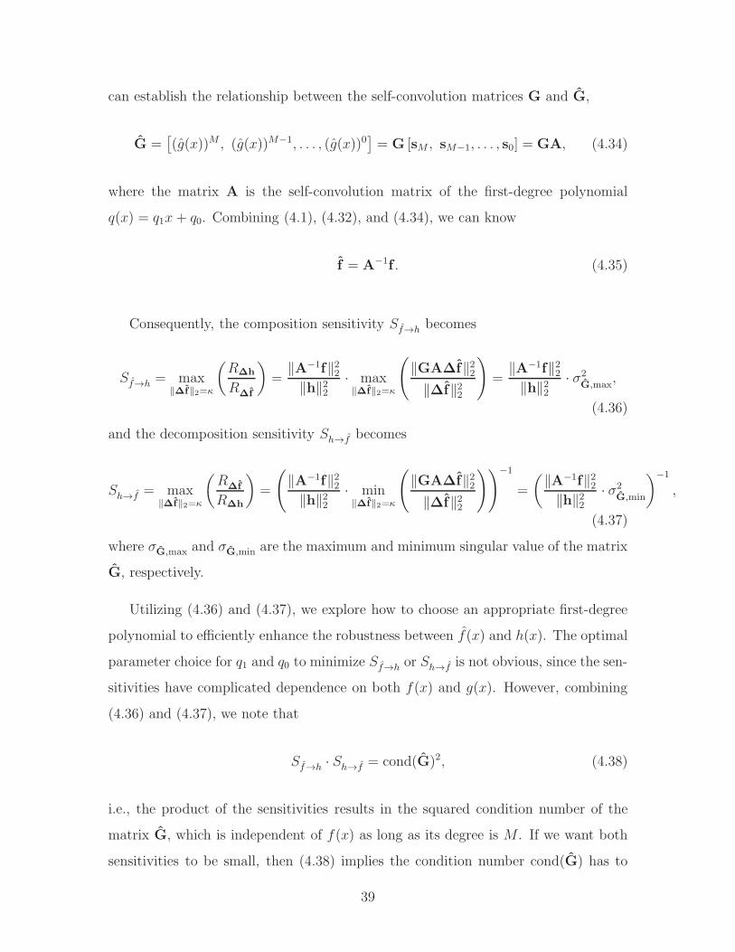
can establish the relationship between the self-convolution matrices G and G,
G =[(g(x))M , (g(x))M−1, . . . , (g(x))0
]= G [sM , sM−1, . . . , s0] = GA, (4.34)
where the matrix A is the self-convolution matrix of the first-degree polynomial
q(x) = q1x+ q0. Combining (4.1), (4.32), and (4.34), we can know
f = A−1f . (4.35)
Consequently, the composition sensitivity Sf→h becomes
Sf→h = max‖∆f‖2=κ
(R∆h
R∆f
)=
‖A−1f‖22‖h‖22
· max‖∆f‖2=κ
(‖GA∆f‖22
‖∆f‖22
)=
‖A−1f‖22‖h‖22
· σ2G,max
,
(4.36)
and the decomposition sensitivity Sh→f becomes
Sh→f = max‖∆f‖2=κ
(R∆f
R∆h
)=
(‖A−1f‖22‖h‖22
· min‖∆f‖2=κ
(‖GA∆f‖22
‖∆f‖22
))−1
=
(‖A−1f‖22‖h‖22
· σ2G,min
)−1
,
(4.37)
where σG,max and σG,min are the maximum and minimum singular value of the matrix
G, respectively.
Utilizing (4.36) and (4.37), we explore how to choose an appropriate first-degree
polynomial to efficiently enhance the robustness between f(x) and h(x). The optimal
parameter choice for q1 and q0 to minimize Sf→h or Sh→f is not obvious, since the sen-
sitivities have complicated dependence on both f(x) and g(x). However, combining
(4.36) and (4.37), we note that
Sf→h · Sh→f = cond(G)2, (4.38)
i.e., the product of the sensitivities results in the squared condition number of the
matrix G, which is independent of f(x) as long as its degree is M . If we want both
sensitivities to be small, then (4.38) implies the condition number cond(G) has to
39

be small. In addition, as shown in (4.5) and (4.7), the condition number cond(G) is
an upper bound for both sensitivities Sf→h and Sh→f , so a small condition number
ensures that these sensitivities are simultaneously small.
To increase robustness, we are interested in the optimal parameters (q∗1, q∗0) that
minimize cond(G), for a given polynomial g(x) and a given degree M .3 It is still
not obvious how to obtain the optimal parameters or to prove the convexity of the
condition number cond(G) with respect to q1 and q0; however, we have the following
parameter selection rule that may approach the minimum value of cond(G).
Approximate Parameter Selection Rule for q(x): Given a polynomial g(x) and
a degree M , the first-degree polynomial q(x) = q1x+ q0 = q1(x+ qr) with parameters
qr = argminqr
‖(g(x) + qr)M‖22, (4.39)
q1 =(‖(g(x) + qr)
M‖22)− 1
2M , (4.40)
q0 = q1 · qr, (4.41)
results in a corresponding matrix G whose condition number is near the minimum
among all first-degree polynomials.
The development of the approximate rule is in Appendix C. The function ‖(g(x)+
qr)M‖22 in (4.39) is convex towards qr, so the parameter qr can be computed efficiently,
and then q1 and q0 are obtained.
The approximate rule can be intuitively explained as follows. If we consider G as a
geometric mapping from the vector spaces of f to that of h, then the condition number
cond(G) is the ratio between the lengths of the longest and the shortest vectors that
are the images of unit vectors. In particular, each unit vector on a coordinate axis
is mapped to a corresponding column of the matrix G. Thus, if the columns of the
matrix G vary significantly in energy, then the condition number is high. In addition,
if two columns of the matrix G are relatively very close in space, then their difference
is a vector with low magnitude, which also leads to a high condition number. Thus,
3Although the matrix G is independent of coefficients of f(x), the degree of f(x) influences thesize of G.
40
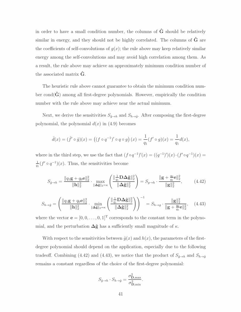
in order to have a small condition number, the columns of G should be relatively
similar in energy, and they should not be highly correlated. The columns of G are
the coefficients of self-convolutions of g(x); the rule above may keep relatively similar
energy among the self-convolutions and may avoid high correlation among them. As
a result, the rule above may achieve an approximately minimum condition number of
the associated matrix G.
The heuristic rule above cannot guarantee to obtain the minimum condition num-
ber cond(G) among all first-degree polynomials. However, empirically the condition
number with the rule above may achieve near the actual minimum.
Next, we derive the sensitivities Sg→h and Sh→g. After composing the first-degree
polynomial, the polynomial d(x) in (4.9) becomes
d(x) = (f ′ ◦ g)(x) =((f ◦ q−1)′ ◦ q ◦ g
)(x) =
1
q1(f ′ ◦ g)(x) =
1
q1d(x),
where in the third step, we use the fact that (f ◦q−1)′(x) = ((q−1)′)(x) ·(f ′◦q−1)(x) =
1q1(f ′ ◦ q−1)(x). Thus, the sensitivities become
Sg→h =‖q1g + q0e‖
22
‖h‖22· max‖∆g‖2=κ
(‖ 1q1D∆g‖22
‖∆g‖22
)= Sg→h ·
‖g + q0q1e‖22
‖g‖22, (4.42)
Sh→g =
(‖q1g + q0e‖
22
‖h‖22· min‖∆g‖2=κ
(‖ 1q1D∆g‖22
‖∆g‖22
))−1
= Sh→g ·‖g‖22
‖g + q0q1e‖22
, (4.43)
where the vector e = [0, 0, . . . , 0, 1]T corresponds to the constant term in the polyno-
mial, and the perturbation ∆g has a sufficiently small magnitude of κ.
With respect to the sensitivities between g(x) and h(x), the parameters of the first-
degree polynomial should depend on the application, especially due to the following
tradeoff. Combining (4.42) and (4.43), we notice that the product of Sg→h and Sh→g
remains a constant regardless of the choice of the first-degree polynomial:
Sg→h · Sh→g =σ2D,max
σ2D,min
.
41

Consequently, these two sensitivities cannot be reduced simultaneously by the same
first-degree polynomial; a decrease in one sensitivity always results in an increase in
the other. Furthermore, we observe that only the ratio qr ,q0q1
affects the sensitivities
between g(x) and h(x) but not the individual q0 or q1; the sensitivity Sg→h decreases
first and then increases with qr, and the ratio to minimize Sg→h is qr = −b0 where
b0 is the constant term in g(x). In addition, for a fixed ratio q0q1
that achieves good
sensitivities between g(x) and h(x), there is still freedom to adjust the values of q0
(or q1) to decrease the sensitivities between f(x) and h(x).
Third, we consider the effects of equivalent composition on sensitivities of the
roots. After the composition with the first-degree polynomial in (4.29), the roots zh
remain the same, but the roots of f(x) become
zf = q(zf) = q1zf + q0,
where zf are the roots of the original polynomial f(x). In a derivation similar to the
above, we finally obtain the sensitivities of the roots for the equivalent compositions:
Szf→zh = Szf→zh ·
‖zf +q0q1‖22
‖zf‖22, (4.44)
Szh→zf
= Szh→zf ·‖zf‖
22
‖zf +q0q1‖22, (4.45)
Sg→zh = Sg→zh ·‖g + q0
q1e‖22
‖g‖22, (4.46)
Szh→g = Szh→g ·‖g‖22
‖g + q0q1e‖22
, (4.47)
where Szf→zh, Szh→zf , Sg→zh, and Szh→g are in (4.22), (4.23), (4.27), and (4.28),
respectively.
The same as the sensitivities between g(x) and h(x), the sensitivities of the roots
have the following two properties. First, the product of two corresponding sensitivities
in the composition and decomposition processes remains a constant for all equivalent
compositions, so it is impossible to decrease both of them simultaneously; second,
the sensitivities of the roots are affected only by the ratio qr = q0q1
rather than the
42
individual values of q1 and q0. Consequently, the optimal choice of parameters has a
tradeoff and depends on the application. In addition, after the determination of the
ratio q0q1
that has acceptable sensitivities of the roots, it is possible to further improve
Sf→h and Sh→f by adjusting q0 (or q1). As for the tendency, we may see that both
Szf→zh and Sg→zh decreases first and then increases with qr; the ratio to minimize
Sg→zh is qr = −b0, which is the same as the ratio to minimize Sg→h, but the ratio qr
to minimize Szf→zh is usually different.
4.3 Simulation Results
In this section, the results of simulations are presented to evaluate sensitivity in
different contexts. Specifically, simulations are shown to evaluate each sensitivity
with polynomials of different degrees, to compare the sensitivities of the coefficients
and those of the roots, and to demonstrate the effectiveness of decreasing sensitivities
with equivalent compositions.
The data in the simulation are generated with the following parameters: The
degrees of both polynomial f(x) and g(x) vary from 2 to 15. For each degree, we create
100 random samples of f(x) and g(x), respectively. For each sample polynomial, the
coefficients are first generated from i.i.d. standard normal distribution, and then the
polynomial is normalized to have unit energy.
4.3.1 Evaluation of the Sensitivities
At each degree of f(x) and g(x), we compose each of the 100 samples of f(x) and
each of the 100 samples of g(x), and then evaluate all the sensitivities for all the
10, 000 compositions. The results are shown in Fig. 4-1 to Fig. 4-8; each figure shows
a certain sensitivity. In these figures, the continuous curve indicates the median of
the sensitivity among the 10, 000 compositions at that degree, and each vertical bar
shows the maximum and the minimum of the sensitivity obtained at that degree in
the simulation.
The first two figures show the sensitivities between the coefficients of f(x) and
43

2 4 6 8 10 12 14 1610
0
105
1010
1015
deg(g(x)) = 7
deg(f(x))
Sen
sitiv
ity S
f→h
Figure 4-1: Coefficient Sensitivity from f(x) to h(x).
2 4 6 8 10 12 14 1610
0
105
1010
1015
deg(g(x)) = 7
deg(f(x))
Sen
sitiv
ity S
h→
f
Figure 4-2: Coefficient Sensitivity from h(x) to f(x).
h(x): the composition sensitivity Sf→h in (3.1) and the decomposition sensitivity
Sh→f in (3.5) are shown in Fig. 4-1 and 4-2, respectively. The degree of g(x) is fixed
to 7, and the degree of f(x) varies from 2 to 15 as indexed by the x-axis. In each
figure, the continuous curve is the median of the sensitivity, and the dashed curve is
the upper bound in (4.5) or (4.7) evaluated with the instance of g(x) that achieves
the maximum sensitivity at each degree. The simulation results demonstrate that the
sensitivities satisfy the theoretical bounds in (4.5) and (4.7). We notice that there
is a considerably large gap between the upper bound for the composition sensitivi-
ty Sf→h and its empirical maximum obtained in the simulation, which indicates the
upper bound in (4.5) is tight in theory but possibly conservative in practice. As for
44
2 4 6 8 10 12 14 16
100
101
102
103
deg(f(x)) = 7
deg(g(x))
Sen
sitiv
ity S
g→
h
Figure 4-3: Coefficient Sensitivity from g(x) to h(x).
2 4 6 8 10 12 14 16
100
102
104
106
deg(f(x)) = 7
deg(g(x))
Sen
sitiv
ity S
h→
g
Figure 4-4: Coefficient Sensitivity from h(x) to g(x).
the tendency of the sensitivities, both sensitivities increase with the increase of the
degree of f(x). In addition, the decomposition sensitivity Sh→f is significantly larger
than the composition sensitivity Sf→h in the simulation, which indicates the compo-
sition process is likely to be more robust than the decomposition process. Although
the sensitivities are large in Fig. 4-1 and 4-2, however, as will be shown in the Sec-
tion 4.3.3, the sensitivities between the coefficients of f(x) to h(x) can be decreased
simultaneously using equivalent compositions, and the robustness can be improved
significantly.
The next two figures correspond to the coefficient sensitivities between g(x) and
h(x): the composition sensitivity Sg→h in (3.3) and the decomposition sensitivity
45

2 4 6 8 10 12 14 1610
−5
100
105 deg(g(x)) = 7
deg(f(x))
Sen
sitiv
ity S
zf→
z h
Figure 4-5: Root Sensitivity from zf to zh.
2 4 6 8 10 12 14 1610
0
102
104
deg(g(x)) = 7
deg(f(x))
Sen
sitiv
ity S
zh→
z f
Figure 4-6: Root Sensitivity from zh to zf .
Sh→g in (3.6) are shown in Fig. 4-3 and 4-4, respectively. The degree of f(x) is fixed
to 7, and the degree of g(x) varies from 2 to 15. The dashed curve in Fig. 4-3 is the
upper bound in (4.13), where g(x) is chosen as the instance that achieves the maxi-
mum sensitivity at each degree. The simulation results show that the upper bound
is satisfied and empirically tight. Furthermore, the decomposition sensitivity Sh→g is
generally larger and increases faster with the degree of g(x) than the composition sen-
sitivity Sg→h. This indicates the composition is more robust than the decomposition
for g(x).
The subsequent two figures show the root sensitivities between f(x) and h(x): Fig.
4-5 shows the composition sensitivity Szf→zh, and Fig. 4-6 shows the decomposition
46

2 4 6 8 10 12 14 16
100
102
104
106
deg(f(x)) = 7
deg(g(x))
Sen
sitiv
ity S
g→
z h
Figure 4-7: Root Sensitivity from g(x) to zh.
2 4 6 8 10 12 14 1610
0
102
104
106 deg(f(x)) = 7
deg(g(x))
Sen
sitiv
ity S
zh→
g
Figure 4-8: Root Sensitivity from zh to g(x).
sensitivity Szh→zf . The degree of f(x) varies from 2 to 15 while the degree of g(x)
is fixed at 7. In contrast to the coefficient sensitivities between f(x) and h(x) that
increase fast with the degree of f(x), the median root sensitivities between zf and
zh have only little increase. This phenomenon indicates potential benefit to use the
roots rather than the coefficients for better robustness in polynomial composition and
decomposition where f(x) has a high degree. The root sensitivities between f(x) and
h(x) is generally more homogeneous and less dependent on the degree of f(x) than
the coefficient sensitivities. We may see this difference from the following example 4:
4Although h(x) has multi-roots in this example, however, as long as g(x) has only single roots,then the multi-roots do not belong to the same group, so the sensitivities Szf→zh and Szh→zf arestill finite.
47

if f(x) = xM , then we can verify the root sensitivities Szf→zh and Szh→zf are the same
value regardless of the degree M , since the ‖zf‖22 and ‖zh‖
22 are both proportional to
M2; however, in the coefficient sensitivities, the size of the matrix G depends on M ,
so the singular values of G may be significantly affected when M increases, which
may result in an increase in the coefficient sensitivities.
The last two figures correspond to the root sensitivities between the coefficients
of g(x) and the roots zh: Fig. 4-7 shows the composition sensitivity Sg→zh, and Fig.
4-8 shows the decomposition sensitivity Szh→g. The degree of g(x) varies from 2 to 15
while the degree of f(x) is fixed at 7. The decomposition sensitivity Szh→g increases
with the degree of g(x), while there does not seem to be such an obviously increasing
tendency for the composition sensitivity Sg→zh.
4.3.2 Comparisons of the Sensitivities
This section shows simulation results comparing the coefficient sensitivities with the
root sensitivities. We perform comparison on sensitivities in four pairs, namely Sf→h
vs Szf→zh, Sh→f vs Szh→zf , Sg→h vs Sg→zh, and Sh→g vs Szh→g; each pair contains a
coefficient sensitivity and a root sensitivity corresponding to the same polynomials
involved. At each degree of f(x) and g(x), we compare the sensitivities within each
pair for each of the 10, 000 composition instances, then we record the percentage of
instances where the root sensitivity is smaller than the coefficient sensitivity. The
results for the four pairs of sensitivities are plotted in Fig. 4-9.
The results seem to support that composition and decomposition using the root
triplet (zf , g, zh) are likely to be more robust than using the coefficient triplet
(f, g, h), when the degrees of polynomials are high. As the degrees of f(x) and
g(x) increase, there are more instances in our simulation where the root sensitivity
is smaller than the corresponding coefficient sensitivity. As we mentioned in Section
4.3.1, between the polynomials f(x) and h(x), since the relationship of the coeffi-
cients in (4.1) involves self-convolution of the polynomial g(x), a perturbation may
be magnified; however, the root sensitivities between zf and zh seem to be more ho-
mogeneous. However, we cannot conclude for every polynomial that the root triplet
48

0
5
10
15
0
5
10
15
85
90
95
100
deg(f(x))
Percentage of instances where S z
f→z
h
< S f→h
deg(g(x))
Per
cent
age
86
88
90
92
94
96
98
(a): Sensitivities from f(x) to h(x),i.e., Sf→h vs Szf→zh
05
1015
05
10150
20
40
60
80
100
deg(f(x))
Percentage of instances where S z
h→z
f
< S h→f
deg(g(x))
Per
cent
age
0
10
20
30
40
50
60
70
80
90
(b): Sensitivities from h(x) to f(x),i.e., Sh→f vs Szh→zf
0
5
10
15
05
1015
50
60
70
80
90
100
deg(f(x))
Percentage of instances where S g→z
h
< S g→h
deg(g(x))
Per
cent
age
45
50
55
60
65
70
75
80
85
90
95
(c): Sensitivities from g(x) to h(x),i.e., Sg→h vs Sg→zh
0
5
10
15
0
5
10
150
20
40
60
80
100
deg(f(x))
Percentage of instances where S z
h→g
< S h→g
deg(g(x))
Per
cent
age
0
10
20
30
40
50
60
70
80
90
(d): Sensitivities from h(x) to g(x),i.e., Sh→g vs Szh→g
Figure 4-9: Comparison between Corresponding Coefficient Sensitivities and RootSensitivities.
has lower sensitivities than the coefficient triplet, since certain multi-roots of h(x)
result in infinite root sensitivities, while all coefficient sensitivities are finite.
4.3.3 Sensitivities of Equivalent Compositions
This section presents simulation results to illustrate the effects of equivalent compo-
sitions on the sensitivities. In particular, we validate the effectiveness of equivalent
49

composition in reducing the sensitivities Sf→h and Sh→f , and we show the perfor-
mance of the approximate rules (4.39)-(4.41) of choosing the first-degree polynomial.
In Fig. 4-10 - Fig. 4-14, we show the dependence of the condition number cond(G)
and all the sensitivities on the parameters of the first-degree polynomial. The degree
of g(x) is 7; polynomial g(x) is chosen as the instance that achieves the maximum
condition number ofG among the 100 random samples (without composing with first-
degree polynomials), which are generated in previous simulations in Section 4.3.1. The
degree of f(x) is chosen as M = 15; f(x) is the polynomial that has the highest sen-
sitivity Sf→h with the g(x) above (without composing with first-degree polynomials)
among the 100 randomly generated instances in previous simulations. In the previous
section, we derive that the sensitivities Sg→h, Sh→g, Szf→zh, Szh→z
f, Sg→zh, and Szh→g
depend only on the ratio qr = q0q1
of the first-degree polynomial. Thus, the x-axis is
qr in Fig. 4-12 - Fig. 4-14 for these sensitivities. In contrast, cond(G), Sf→h, and
Sh→f depend on both q1 and q0. For consistency with the other sensitivities, we plot
cond(G), Sf→h, and Sh→f with respect to q1 and qr = q0q1. The range of q1 and qr
are [0.9, 1.9] and [−1.4,−0.4], respectively.
Fig. 4-10 indicates that there is an optimal q∗(x) that achieves the minimum
0.9 1.1 1.3 1.5 1.7 1.9
−1.4−1.2−1−0.8−0.6−0.410
0
103
106
109
q1qr =q0q1
cond(G
)
Figure 4-10: The Condition Number cond(G) with Different q1 and qr, where qr =q0q1.
50
0.91.11.31.51.71.9
−1.4−1.2
−1−0.8
−0.6−0.4
100
103
106
109
q1qr =q0q1
SensitivitySh→
f
(b) Sh→f
0.91.11.31.51.71.9
−1.4−1.2 −1−0.8−0.6−0.4
100
103
106
109
1012
q1qr =q0q1
SensitivitySf→
h
(a) Sf→h
Figure 4-11: The Sensitivities Sf→h and Sh→f with Different q1 and qr.
condition number cond(G); in this example, the optimal first-order polynomial has
parameters as q∗r = −0.8563, q∗1 = 1.3973, and q∗0 = −1.1965. As the parameters q1
and qr deviate from the optimal point, the condition number increases rapidly. In
Fig. 4-11, the sensitivities Sf→h and Sh→f also have their respective minimum points,
which are near q∗(x). Thus, these figures show that we can choose a proper q(x)
to have low sensitivities in both the composition and the decomposition operations,
between the coefficients of f(x) and h(x).
In contrast, in each pair of sensitivities in Fig. 4-12 - Fig. 4-14, an decrease
in one sensitivity results in an increase in the other; this phenomenon is consistent
with our derivation in Section 4.2: the product of the two sensitivities remains a
constant regardless of qr. In addition, as discussed in Section 4.2, the composition
sensitivities decrease at first and then increase (the range of qr does not include the
minimum point for Szf→zh in Fig. 4-13); the sensitivities Sg→h and Sg→zh share the
same optimal value for qr.
Fig. 4-15 shows the condition number with polynomials of different degrees, and
tests the performance of the approximate rules in (4.39)-(4.41). In Fig. 4-15 (a) and
(b), the polynomial g(x) has degree 7, and we use the 100 randomly generated in-
stances of g(x) in previous sections; the degree5 of f(x) varies from 2 to 15. The three
5Although the matrix G is independent of coefficients of f(x), the degree of f(x) influences thesize of G.
51
curves in 4-15 (a) are obtained as follows: for each degree M , we pick the polynomial
g(x) that achieves the maximum original condition number cond(G) within the 100
samples (without composing with first-degree polynomials); with the instance of g(x)
that we pick, the dash-dot line denotes the original condition number, the dotted
line denotes the minimum condition number by composing with the optimal first-
degree polynomial q∗(x), and the continuous line denotes the condition number by
composing with the first-degree polynomial q(x) proposed by the approximate rules
(4.39)-(4.41). For the instance of g(x) at each degree, the optimal first-degree poly-
nomial q∗(x) to minimize cond(G) is obtained by brute force search. To show the
performance of the approximate rule clearly, we magnify Fig. 4-15 (a) into Fig. 4-15
(b), but without the curve of the original condition number. The above description
also applies to Fig. 4-15 (c) and (d), but the polynomial g(x) has degree 15 rather
than 7 for these figures.
The figures demonstrate that the equivalent composition efficiently reduces the
condition number G, and the approximate rules are considerably effective to achieve
a nearly minimum condition number. In Fig. 4-15 (a) and (c), compared with the
rapid growth of the original condition number with the degree M , the corresponding
minimum condition number has only considerably small increase. At each degreeM in
Fig. 4-15 (b) and (d), the condition number of equivalent composition by composing
with q(x) that is proposed by the approximate rules is considerably near the actual
minimum value. Thus, the approximate rules (4.39)-(4.41) are considerably effective
in practice.
As shown in (4.5) and (4.7), the squared condition number of G is an upper bound
for both sensitivities Sf→h and Sh→f . In our simulation, since the minimum condition
number can be reduced to less than 2.5 with proper equivalent composition, these
two sensitivities also become considerably low, which indicates an improvement of
robustness.
52

−1.4 −1.2 −1 −0.8 −0.6 −0.410
1
102
103
qr =q0q1
Sensitivities
Sg→h
Sh→ g
Figure 4-12: The Sensitivities Sg→h and Sh→g with Different qr.
−1.4 −1.2 −1 −0.8 −0.6 −0.4
100
101
102
qr =q0q1
Sensitivities
Szf→zh
Szh→zf
Figure 4-13: The Sensitivities Szf→zh and Szh→z
fwith Different qr.
−1.4 −1.2 −1 −0.8 −0.6 −0.4
100
101
102
qr =q0q1
Sen
sitivities
Sg→zh
Szh→ g
Figure 4-14: The Sensitivities Sg→zh and Szh→g with Different qr.
53

2 4 6 8 10 12 14 1610
0
102
104
106
108
M
cond(G
)
deg(g(x))=7
OriginalMinimumRule
(a): deg(g) = 7
2 4 6 8 10 12 14 161
1.2
1.4
1.6
1.8
2
M
cond(G
)
deg(g(x))=7
MinimumRule
(b): deg(g) = 7 (Magnified)
2 4 6 8 10 12 14 1610
0
102
104
106
M
cond(G
)
deg(g(x))=15
OriginalMinimumRule
(c): deg(g) = 15
2 4 6 8 10 12 14 161
1.5
2
2.5
3
M
cond(G
)
deg(g(x))=15
MinimumRule
(d): deg(g) = 15 (Magnified)
Figure 4-15: Comparison of the Condition Number of G among the Original Value,the Minimum Value, and the Value Achieved with the Approximate Rules (4.39)-(4.41).
54

Chapter 5
Exact Decomposition Algorithms
In this chapter, algorithms are discussed for the exact decomposition for polynomials
that are known to be decomposable. The associated simulation results are also pre-
sented. Three algorithms are shown for the problems as defined in Section 3.2: one
of the algorithms has coefficients as input corresponding to Problem 1, while the oth-
er two have roots as input corresponding to Problem 2. Simulations are performed
to compare the new algorithm developed in Section 5.2.3 with two other existing
algorithms. 1
In the development of the methods, an assumption is made without loss of gen-
erality. Specifically, in this chapter, we assume that all the polynomials f(x), g(x),
and h(x) are monic, and the constant term in g(x) is zero; i.e.,
aM = bN = cMN = 1, and b0 = 0, (5.1)
where ai, bi, and ci are the coefficients of the term xi in f(x), g(x), and h(x), respec-
tively.
The validity of this assumption results from the equivalent compositions with first-
degree polynomials. As mentioned in Sections 2.1 and 4.2, for an arbitrary first-degree
polynomial q(x) = q1x + q0, it holds that f ◦ g = f ◦ g, where f(x) = (f ◦ q−1)(x)
1The first two algorithms in this chapter and the associated simulation results are included in [11]by S. Demirtas, G. Su, and A. V. Oppenheim.
55

and g(x) = (q ◦ g)(x). Thus, by choosing a proper q(x), we can set g(x) as a monic
polynomial with a constant term of zero. Consequently, there always exists a way of
decomposing h(x) as (f ◦ g)(x) such that bN = 1 and b0 = 0. This case implies that
cMN = aMbMN = aM , so the leading coefficients of f(x) and h(x) are the same. Thus,
f(x) and h(x) can be scaled to monic polynomials simultaneously. This concludes
the validation of our assumption.
As a byproduct, equivalent compositions with linear functions also imply that
the degrees of freedom of decomposable h(x) (with fixed M and N) are at most
(M + 1) + (N + 1) − 2 = M + N , which is two fewer than the total number of
coefficients in f(x) and g(x).
5.1 Problem 1: Exact Decomposition with Coeffi-
cients as Input
An algorithm for exact decomposition with coefficients as input was proposed by
Kozen and Landau in [17]. This algorithm employs the fact that the N highest
degree terms of h(x) depend only on the coefficients of g(x) and the highest degree
term of f(x). By solving a system of equations iteratively, the coefficients of g(x)
can be obtained in the descending order of the degrees of terms. After obtaining
g(x), the coefficients of f(x) can be solved by a projection method due to the linear
relationship between h(x) and f(x) as shown in (4.1).
The coefficients of several highest degree terms in h(x) have the expressions:
cMN = aMbMN
cMN−1 =
(M
1
)aMb
M−1N bN−1
cMN−2 =
(M
2
)aMb
M−2N b2N−1 +
(M
1
)aMb
M−1N bN−2
cMN−3 =
(M
3
)aMb
M−3N b3N−1 +
(M
1
)(M − 1
1
)aMb
M−2N bN−1bN−2 +
(M
1
)aMb
M−1N bN−3
These equations imply the theorem that is observed by Kozen and Landau [17]:
56

Theorem 5.1. [17]. For 1 ≤ k ≤ N − 1, the coefficient cMN−k in h(x) satisfies
cMN−k = µk (aM , bN , bN−1 . . . bN−k+1) +
(M
1
)aMb
M−1N bN−k, (5.2)
where µk (aM , bN , bN−1 . . . bN−k+1) is a polynomial of aM and of the coefficients of
terms with degrees higher than bN−kxN−k in g(x).
This theorem is directly implied by the fact that the terms cMN−kxMN−k (1 ≤
k ≤ N − 1) in h(x) can be generated only by aMg(x)M , i.e., the highest degree term
in f(x). Using multinomial expansion, we can further see that cMN−k is independent
of bN−j where k < j ≤ N . A detailed discussion can be found in [17], which has the
same core idea as the fact above.
Theorem 5.1 shows clearly that, after aM , bN , bN−1 . . . bN−k+1 are obtained, a linear
equation can be constructed with respect to bN−k. Thus, the coefficients of g(x) can
be obtained one by one from the highest degree term to the lowest; in this process of
coefficient unraveling, only the N highest degree terms in h(x) are used.
After g(x) is obtained, the determination of f(x) can be accomplished by the
solution to the linear equations (4.1):
f = G†h, (5.3)
where G† = (GTG)−1GT is the pseudo-inverse matrix of G, and the matrix G is the
self-convolution matrix as defined in (4.2).
In summary, the algorithm for exact decomposition with coefficients as input is
stated as follows:
Coefficient-Unraveling Algorithm [17]
(1) for k = 1 to N − 1
(2) Calculate µk (aM , bN , bN−1, . . . , bN−k+1)
(3) Obtain bN−k = (cMN−k − µk (aM , bN , bN−1, . . . , bN−k+1))/(MaM)
(4) endfor
(5) Construct the matrix G as defined in (4.2).
57

(6) Solve the coefficients of f(x) by (5.3).
5.2 Problem 2: Exact Decomposition with Roots
as Input
This section presents two algorithms for exact decomposition with roots as input: the
first algorithm is based on the algorithm by Aubry and Valibouze [20]; we present
a new algorithm based on grouping the roots of the composed polynomial. Both
algorithms use the structure of the roots of a decomposable polynomial, as well as
the relationship between the coefficients and the roots of a polynomial. The properties
of the roots of a decomposable polynomial are first stated in Section 5.2.1, and then
the two algorithms are presented in Sections 5.2.2 and 5.2.3, respectively.
5.2.1 Properties of Roots of a Decomposable Polynomial
As mentioned in Section 4.1.2, we can partition all the roots of h(x) into M groups
A1, A2, . . . , AM , and the roots in each group correspond to the same root of f(x).
The same as in Section 4.1.2, we denote the roots of f(x) and h(x) as zf (i) (1 ≤ i ≤
M) and zh(k) (1 ≤ k ≤ MN), respectively. Then, the roots zh(k) in the group Ai
all satisfy gi(zh(k)) = 0, where gi(x) = g(x) − zf (i) is a polynomial with a different
constant term from g(x). Without loss of generality, we assume all polynomials
involved are monic.
Since each gi(x) has the same coefficients except for the constant term, Theorem
5.2 is implied by Vieta’s theorem that states the relationship between the coefficients
and the roots of a polynomial [27].
Theorem 5.2. [27]. For each j = 1, 2, ..., N − 1, the j-th elementary symmetric
function σj(·) has the same value on all groups Ai (1 ≤ i ≤ M), where σj(Ai) is
58

defined as
σj(Ai) =∑
k1<k2<···<kj∈Ai
zh(k1)zh(k2)zh(k3) · · · zh(kj), 1 ≤ j ≤ N − 1. (5.4)
Newton’s identities [28], which show the relationship between the elementary sym-
metric functions and the power summations of the roots of a polynomial, imply the
validity of Theorem 5.3 from Theorem 5.2 [20].
Theorem 5.3. [20]. For each j = 1, 2, ..., N −1, the j-th power summation of roots
sj(·) has the same value on all groups Ai (1 ≤ i ≤M), where sj(Ai) is defined as
sj(Ai) =∑
k∈Ai
(zh(k))j , 1 ≤ j ≤ N − 1. (5.5)
5.2.2 Root-Power-Summation Algorithm
Based on Theorem 5.3, an algorithm was proposed in [20] in order to determine a
polynomial g(x) from its self-convolution (g(x))N . In fact, this algorithm can also be
applied to the general problem of determining g(x) from the composition (f ◦ g)(x).
The algorithm in [20] has the following principles. Since the power summations
sj(Ai) in (5.5) are equal for each group Ai (i = 1, 2, ...,M), they can be directly
computed by
sj , sj(Ai) =1
M
MN∑
k=1
(zh(k))j , 1 ≤ j ≤ N − 1. (5.6)
Then, the coefficients of g(x) are obtained by using Newton’s identities [20, 28].
Next, we need to determine the component f(x). An elementary way is to first
obtain the roots of f(x) by clustering g(zh(k)) for k = 1, 2, . . . ,MN and using the
largestM clusters; then, f(x) is solved by f(x) =∏M
i=1(x−zf (i)). However, since nu-
merical errors in the input roots may be magnified and cause the final reconstruction
of f(x) to be inaccurate, the description above is just a basic implementation of the
59
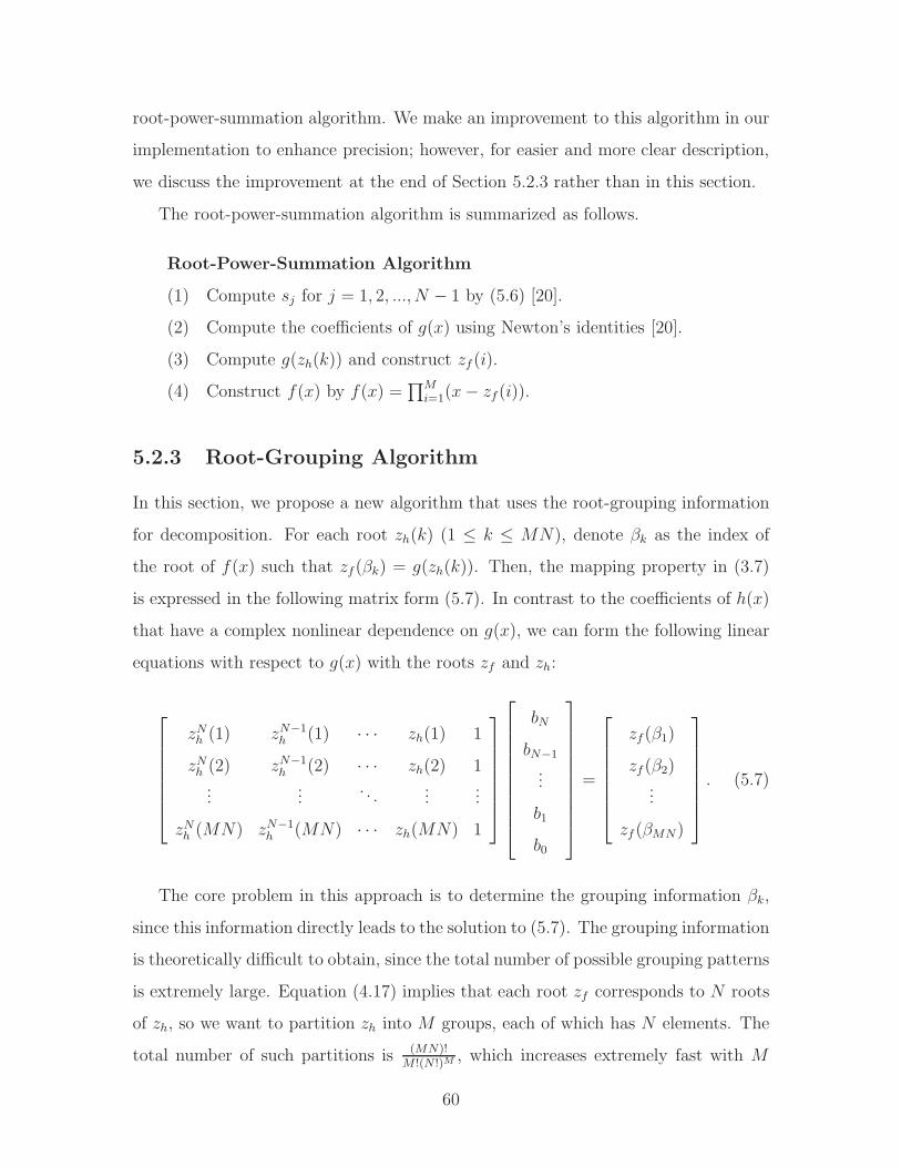
root-power-summation algorithm. We make an improvement to this algorithm in our
implementation to enhance precision; however, for easier and more clear description,
we discuss the improvement at the end of Section 5.2.3 rather than in this section.
The root-power-summation algorithm is summarized as follows.
Root-Power-Summation Algorithm
(1) Compute sj for j = 1, 2, ..., N − 1 by (5.6) [20].
(2) Compute the coefficients of g(x) using Newton’s identities [20].
(3) Compute g(zh(k)) and construct zf (i).
(4) Construct f(x) by f(x) =∏M
i=1(x− zf (i)).
5.2.3 Root-Grouping Algorithm
In this section, we propose a new algorithm that uses the root-grouping information
for decomposition. For each root zh(k) (1 ≤ k ≤ MN), denote βk as the index of
the root of f(x) such that zf(βk) = g(zh(k)). Then, the mapping property in (3.7)
is expressed in the following matrix form (5.7). In contrast to the coefficients of h(x)
that have a complex nonlinear dependence on g(x), we can form the following linear
equations with respect to g(x) with the roots zf and zh:
zNh (1) zN−1h (1) · · · zh(1) 1
zNh (2) zN−1h (2) · · · zh(2) 1
......
. . ....
...
zNh (MN) zN−1h (MN) · · · zh(MN) 1
bN
bN−1
...
b1
b0
=
zf (β1)
zf (β2)...
zf (βMN)
. (5.7)
The core problem in this approach is to determine the grouping information βk,
since this information directly leads to the solution to (5.7). The grouping information
is theoretically difficult to obtain, since the total number of possible grouping patterns
is extremely large. Equation (4.17) implies that each root zf corresponds to N roots
of zh, so we want to partition zh into M groups, each of which has N elements. The
total number of such partitions is (MN)!M !(N !)M
, which increases extremely fast with M
60

and N . Thus, searching all possible grouping patterns is impractical due to its high
computational complexity.
However, Theorem 5.3 constrains the possible grouping patterns and effectively
decreases the computational complexity in practice. We propose an approach that
formulates the grouping pattern as a mixed integer program. There are M steps
in this approach; in each step, we determine the N roots in a group, and then we
remove them from the roots that remain to be grouped. To determine the roots that
form a new group, we introduce binary indicators δk for each zh(k) that has not been
grouped yet, and the following mixed integer program (MIP) is constructed:
min 0 (5.8)
s. t.∑
k∈S
δk · (zh(k))j = sj , ∀j = 1, 2, ..., N − 1, (5.9)
∑
k∈S
δk = N, (5.10)
δk ∈ {0, 1}, ∀k ∈ S.
The set S is those roots zh(k) that have not been grouped. If δk = 1, then zh(k) is in
the newly constructed group; otherwise, zh(k) remains not grouped. The constraint
(5.9) is due to Theorem 5.3, and the constraint (5.10) results from the fact that each
group has N roots. The values of sj in (5.9) are calculated by (5.6). Due to numerical
errors in implementation, the constraint (5.9) can be relaxed to
∣∣∣∣∣∑
k∈S
δk · (zh(k))j − sj
∣∣∣∣∣ ≤ ǫ|sj|, ∀j = 1, 2, ..., N − 1, (5.11)
for a small ǫ; furthermore, since the roots zh(k) are mostly complex numbers, the
left-hand-side of (5.11) for each j is implemented for the real part and the imaginary
part, respectively. 2 Since we are interested only in the binary points in the feasible
region, the cost function can be arbitrary and we set it as 0 for simplicity. After
2In contrast, the right-hand-side of (5.11) is a constant for the optimization problem, so we donot separate the real and imaginary parts of it; in addition, |sj | in (5.11) is the magnitude of thecomplex number sj.
61

the mixed integer optimization problem in (5.8) has been solved for M times, the
grouping information can be fully determined.
An improvement is performed on the procedure above to decrease time complexity
for obtaining the grouping information. In fact, we do not need to solve the opti-
mization problem in (5.8) for M times; instead, we only solve (5.8) for one time and
get one group of roots. Then we can construct g(x) as follows:
g(x) =∏
k∈A1
(x− zh(k))− (−1)N∏
k∈A1
zh(k), (5.12)
Although numerical errors may cause (5.12) to be a rough reconstruction, however,
we may still use (5.12) to determine the grouping information. The roots zh in one
group should have the same value of g(zh), so we can cluster g(zh) to obtain the
grouping information of zh.
After obtaining the full grouping information, we consider the construction of
g(x) and zf . Theoretically, we can construct g(x) in (5.12) with any one group,
then the roots of f(x) are computed by zf(i) = g(zh(k)), k ∈ Ai, 1 ≤ i ≤ M .
However, accumulation of numerical error may cause the direct expansion (5.12) to
be inaccurate. To enhance robustness and precision, we utilize the linear relationship
in (5.7) and form the following linear program to solve zf (i) and g(x):
minbj ,zf (i)
M∑
i=1
∑
k∈Ai
|ψi,k| (5.13)
s. t. ψi,k =
N−1∑
j=1
(zh(k))j · bj + (zh(k))
N − zf (i),
for i = 1, 2, ...,M, k ∈ Ai. (5.14)
The cost function for this linear program is the total deviation from g(zh(k)) to zf (i)
where zh(k) belongs to the group Ai; the deviation should be zero in theory without
numerical error. The grouping information Ai has been obtained by solving the mixed
integer program in (5.8). Since the roots zh(k) and zf (i) are mostly complex numbers,
we implement (5.14) for the real and imaginary parts, respectively; then, the terms
62

in the cost function are implemented as |ψi,k| , |Re {ψi,k}|+ |Im {ψi,k}|. In addition
to the constraints listed above, we also constrain that the roots zf that correspond
to conjugate pairs of zh are also in a conjugate pair, which ensures that f(x) has real
coefficients.
The complete algorithm is summarized as follows:
Root-Grouping Algorithm
(1) Set S = {1, 2, ...,MN}, and compute sj (1 ≤ j ≤ N − 1) from (5.6).
(2) Solve the integer program in (5.8).
(3) Construct the first group A1 = {k ∈ S | δk = 1}.
(4) Obtain a rough reconstruction of g(x) from (5.12).
(5) Determine the full grouping information Ai (1 ≤ i ≤M) by clustering g(zh).
(6) Construct precise g(x) and zf (i) from linear optimization (5.13).
(7) Construct f(x) by f(x) =∏M
i=1(x− zf (i)).
Compared to the high complexity of a number of integer programming problems,
the efficiency in practice of formulation (5.8) is usually high.
As a last comment, the technique of reconstructing g(x) and zf from the linear
program in (5.13) is also applicable to the root-power-summation algorithm, which
can improve the overall precision. In that algorithm, we have a rough reconstruction
of g(x) using the power summation of roots (5.6) and Newton’s identity [20]. Then,
we can obtain the grouping information of roots zh by clustering g(zh). With the
grouping information, we finally use the linear program in (5.13) to solve g(x) and
zf , which enhances numerical performance.
5.3 Evaluation of the Exact Decomposition Algo-
rithms
This section presents a comparison between the three exact decomposition algorithms
with respect to the success rates of f(x), g(x), and h(x) in the decomposition. From
the coefficients or the roots of a decomposable polynomial h(x) = (f ◦ g)(x), the
63

three algorithms obtain the components f(x) and g(x), and then we compose f(x)
and g(x) into h(x) = (f ◦ g)(x). The errors in this decomposition process are defined
as
errp(x) = p(x)− p(x), for p(x) = f(x), g(x), or h(x).
The signal to error ratios (SER) are defined as
SERp , 20 log10
(‖p(x)‖2
‖errp(x)‖2
), for p(x) = f(x), g(x), or h(x).
The criterion of successful decomposition is chosen as SERp ≥ 80dB in the simulation,
for p(x) = f(x), g(x), or h(x).
In the simulation, the degrees of f(x) and g(x) are equal and vary from 5 to 75 with
increments of 5; the corresponding degrees of h(x) vary from 25 to 5625. For each fixed
degree, we generate 100 samples of h(x) by composing monic polynomial components
f(x) and g(x) with coefficients of i.i.d. standard Gaussian distribution (except for the
leading terms and the constant terms: f(x) and g(x) are both monic polynomials,
and g(x) has a constant term of zero). The roots zf and zh are computed, and then
zh are sorted into random order. Then all three algorithms perform decomposition
on these samples. The details of parameter setting for the algorithms are as follows.
In the algorithms working with roots, two reconstructed roots g(zh) are considered to
belong to one cluster (i.e., correspond to the same zf ) if the distance between them
is lower than a threshold, for which we use 10−3. In the root-grouping algorithm, the
mixed integer optimization problem (5.8) is solved by the CPLEX software where we
set the time limit for the MIP as 2 minutes, and the parameter ǫ in (5.11) is chosen as
10−11 in our simulation. For each algorithm, we record its successful decomposition
rates within the sample polynomials according to the criterion above; the results for
f(x), g(x), and h(x) are plotted in Fig. 5-1 (a), (b), and (c), respectively.
Figure 5-1 indicates that among these three algorithms, the root-power-summation
algorithm has the best performance, followed by the root-grouping algorithm; the
coefficient-unraveling algorithm has the lowest successful decomposition rate. For ex-
ample, when M = N = 50, the coefficient-unraveling algorithm fails to decompose
64
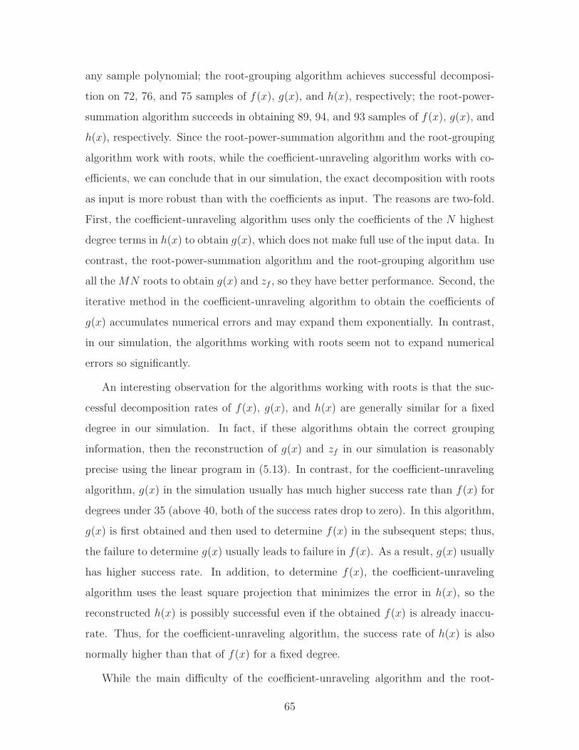
any sample polynomial; the root-grouping algorithm achieves successful decomposi-
tion on 72, 76, and 75 samples of f(x), g(x), and h(x), respectively; the root-power-
summation algorithm succeeds in obtaining 89, 94, and 93 samples of f(x), g(x), and
h(x), respectively. Since the root-power-summation algorithm and the root-grouping
algorithm work with roots, while the coefficient-unraveling algorithm works with co-
efficients, we can conclude that in our simulation, the exact decomposition with roots
as input is more robust than with the coefficients as input. The reasons are two-fold.
First, the coefficient-unraveling algorithm uses only the coefficients of the N highest
degree terms in h(x) to obtain g(x), which does not make full use of the input data. In
contrast, the root-power-summation algorithm and the root-grouping algorithm use
all theMN roots to obtain g(x) and zf , so they have better performance. Second, the
iterative method in the coefficient-unraveling algorithm to obtain the coefficients of
g(x) accumulates numerical errors and may expand them exponentially. In contrast,
in our simulation, the algorithms working with roots seem not to expand numerical
errors so significantly.
An interesting observation for the algorithms working with roots is that the suc-
cessful decomposition rates of f(x), g(x), and h(x) are generally similar for a fixed
degree in our simulation. In fact, if these algorithms obtain the correct grouping
information, then the reconstruction of g(x) and zf in our simulation is reasonably
precise using the linear program in (5.13). In contrast, for the coefficient-unraveling
algorithm, g(x) in the simulation usually has much higher success rate than f(x) for
degrees under 35 (above 40, both of the success rates drop to zero). In this algorithm,
g(x) is first obtained and then used to determine f(x) in the subsequent steps; thus,
the failure to determine g(x) usually leads to failure in f(x). As a result, g(x) usually
has higher success rate. In addition, to determine f(x), the coefficient-unraveling
algorithm uses the least square projection that minimizes the error in h(x), so the
reconstructed h(x) is possibly successful even if the obtained f(x) is already inaccu-
rate. Thus, for the coefficient-unraveling algorithm, the success rate of h(x) is also
normally higher than that of f(x) for a fixed degree.
While the main difficulty of the coefficient-unraveling algorithm and the root-
65

power-summation algorithm is numerical errors, the main challenge for the root-
grouping algorithm is solving the mixed integer program in (5.8). The success rates
of all algorithms generally decrease as the degrees M and N increase, since both
numerical errors in all algorithms and the scale of MIP in the root-grouping algorithm
increase with the degrees. However, the solution to the MIP problem is considerably
efficient as compared with general MIP problems, especially when we take its scale
into account. For example, when M = N = 30, there are 900 binary variables in the
MIP problem, and there are 9.80× 1055 possible patterns for the first group without
considering the constraints on the power summations. However, the constraints from
Theorem 5.3 efficiently shrink the feasible region and lower down the complexity so
that the grouping information is obtained for 97 samples within the time limit of
2 minutes. Moreover, the efficiency of the MIP formulation depends on individual
samples of polynomial; in general, we speculate that our MIP formulation in (5.8)
may be more efficient if the absolute values of roots |zh| do not have a large range.
This speculation results from the constraints (5.11). If there are two roots with a
very large and a very small absolute value, respectively, then the high powers of the
two roots have significantly different magnitudes. Thus, the power of the small root
is susceptible to numerical errors and does not have much influence on the power
summations when j is large. Consequently, if the large root is in the new group, it is
not effective to decide whether the small root belongs to the group using the constraint
(5.11) with a large j. In other words, such constraints may become ineffective to
shrink the feasible region, and the computational complexity may not get efficiently
decreased. In contrast, if all the roots have similar magnitudes, then it is likely that
the power summation constraint (5.11) for each power j effectively shrinks the binary
points in the feasible region, which results in higher overall efficiency.
66
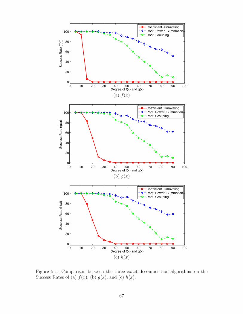
0 10 20 30 40 50 60 70 80 90 1000
20
40
60
80
100
Degree of f(x) and g(x)
Suc
cess
Rat
e (f
(x))
Coefficient−UnravelingRoot−Power−SummationRoot−Grouping
(a) f(x)
0 10 20 30 40 50 60 70 80 90 1000
20
40
60
80
100
Degree of f(x) and g(x)
Suc
cess
Rat
e (g
(x))
Coefficient−UnravelingRoot−Power−SummationRoot−Grouping
(b) g(x)
0 10 20 30 40 50 60 70 80 90 1000
20
40
60
80
100
Degree of f(x) and g(x)
Suc
cess
Rat
e (h
(x))
Coefficient−UnravelingRoot−Power−SummationRoot−Grouping
(c) h(x)
Figure 5-1: Comparison between the three exact decomposition algorithms on theSuccess Rates of (a) f(x), (b) g(x), and (c) h(x).
67

68

Chapter 6
Approximate Decomposition
Algorithms
In this chapter, we present and evaluate algorithms for approximate polynomial de-
composition. In contrast to exact decomposition which can be thought of as a problem
of identification, approximate decomposition corresponds to modeling. Four algo-
rithms are explored for the problems defined in Section 3.3: three of the algorithms
are for Problem 3 for which the input is the coefficients, and the fourth is for Problem
4 for which the input is the roots. Simulation results are presented to evaluate the
algorithms. 1
6.1 Problem 3: Approximate Decomposition with
Coefficients as Input
This section presents three algorithms for the approximate decomposition problem
with polynomial coefficients as input, as stated in Section 3.3. The algorithms belong
to two categories: the iterative mean square approximation algorithm and algorithms
based on the Ruppert matrix.
1The first three algorithms in this chapter and the associated simulation results are includedin [11] by S. Demirtas, G. Su, and A. V. Oppenheim.
69

6.1.1 Iterative Mean Square Approximation Algorithm
This approach was proposed by Corless et al. in [18]; it updates the polynomials f(x)
and g(x) iteratively, where the update is achieved by approximate linearization and
mean square projection. Since the composition is linear with respect to f(x), if we
fix g(x) and want to obtain an approximate polynomial f(x) to minimize the error
energy ‖h(x)− (f ◦ g)(x)‖22, then the optimal f(x) is the mean square projection as
given in (5.3). However, if we fix f(x) and want to derive the optimal g(x) to minimize
the error energy, the problem is much more challenging since the composition is non-
linear with respect to g(x). If the input polynomial is near a decomposable one, then
we may apply the Taylor approximation
h(x)− (f ◦ (g +∆g))(x) ≈ h(x)− (f ◦ g)(x)− (f ′ ◦ g) (x) ·∆g(x), (6.1)
where f ′(x) is the derivative of f(x). If we denote r(x) = h(x)− (f ◦ g)(x), then (6.1)
can be presented in an equivalent matrix formulation
D ·∆g ≈ r, (6.2)
where the matrix D is the Teoplitz matrix in (4.11). Thus, we can apply the mean
square projection to obtain ∆g(x), where g(x) +∆g(x) approximately minimizes the
error energy ‖h(x)− (f ◦ (g +∆g))(x)‖22:
∆g = D†r. (6.3)
If the input polynomial is near a decomposable polynomial, then the coefficient-
unraveling algorithm for exact decomposition [17] in Section 5.1 would possibly have
outputs f(x) and g(x) that are sufficiently near the optimal polynomials. Thus, the
coefficient-unraveling algorithm can provide initial values for f(x) and g(x). In the
iteration, we iteratively use linear projections (5.3) and (6.3) to update f(x) and g(x),
respectively. The algorithm is summarized as follows:
70
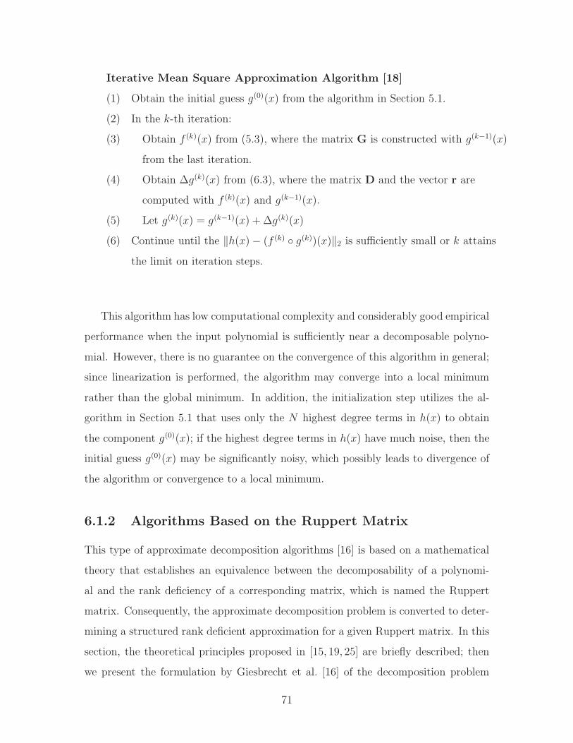
Iterative Mean Square Approximation Algorithm [18]
(1) Obtain the initial guess g(0)(x) from the algorithm in Section 5.1.
(2) In the k-th iteration:
(3) Obtain f (k)(x) from (5.3), where the matrix G is constructed with g(k−1)(x)
from the last iteration.
(4) Obtain ∆g(k)(x) from (6.3), where the matrix D and the vector r are
computed with f (k)(x) and g(k−1)(x).
(5) Let g(k)(x) = g(k−1)(x) + ∆g(k)(x)
(6) Continue until the ‖h(x)− (f (k) ◦ g(k))(x)‖2 is sufficiently small or k attains
the limit on iteration steps.
This algorithm has low computational complexity and considerably good empirical
performance when the input polynomial is sufficiently near a decomposable polyno-
mial. However, there is no guarantee on the convergence of this algorithm in general;
since linearization is performed, the algorithm may converge into a local minimum
rather than the global minimum. In addition, the initialization step utilizes the al-
gorithm in Section 5.1 that uses only the N highest degree terms in h(x) to obtain
the component g(0)(x); if the highest degree terms in h(x) have much noise, then the
initial guess g(0)(x) may be significantly noisy, which possibly leads to divergence of
the algorithm or convergence to a local minimum.
6.1.2 Algorithms Based on the Ruppert Matrix
This type of approximate decomposition algorithms [16] is based on a mathematical
theory that establishes an equivalence between the decomposability of a polynomi-
al and the rank deficiency of a corresponding matrix, which is named the Ruppert
matrix. Consequently, the approximate decomposition problem is converted to deter-
mining a structured rank deficient approximation for a given Ruppert matrix. In this
section, the theoretical principles proposed in [15, 19, 25] are briefly described; then
we present the formulation by Giesbrecht et al. [16] of the decomposition problem
71
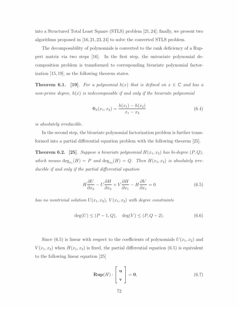
into a Structured Total Least Square (STLS) problem [21,24]; finally, we present two
algorithms proposed in [16, 21, 23, 24] to solve the converted STLS problem.
The decomposability of polynomials is converted to the rank deficiency of a Rup-
pert matrix via two steps [16]. In the first step, the univariate polynomial de-
composition problem is transformed to corresponding bivariate polynomial factor-
ization [15, 19], as the following theorem states.
Theorem 6.1. [19]. For a polynomial h(x) that is defined on x ∈ C and has a
non-prime degree, h(x) is indecomposable if and only if the bivariate polynomial
Φh(x1, x2) =h(x1)− h(x2)
x1 − x2(6.4)
is absolutely irreducible.
In the second step, the bivariate polynomial factorization problem is further trans-
formed into a partial differential equation problem with the following theorem [25].
Theorem 6.2. [25]. Suppose a bivariate polynomial H(x1, x2) has bi-degree (P,Q),
which means degx1(H) = P and degx2
(H) = Q. Then H(x1, x2) is absolutely irre-
ducible if and only if the partial differential equation
H∂U
∂x2− U
∂H
∂x2+ V
∂H
∂x1−H
∂V
∂x1= 0 (6.5)
has no nontrivial solution U(x1, x2), V (x1, x2) with degree constraints
deg(U) ≤ (P − 1, Q), deg(V ) ≤ (P,Q− 2). (6.6)
Since (6.5) is linear with respect to the coefficients of polynomials U(x1, x2) and
V (x1, x2) when H(x1, x2) is fixed, the partial differential equation (6.5) is equivalent
to the following linear equation [25]
Rup(H) ·
u
v
= 0, (6.7)
72
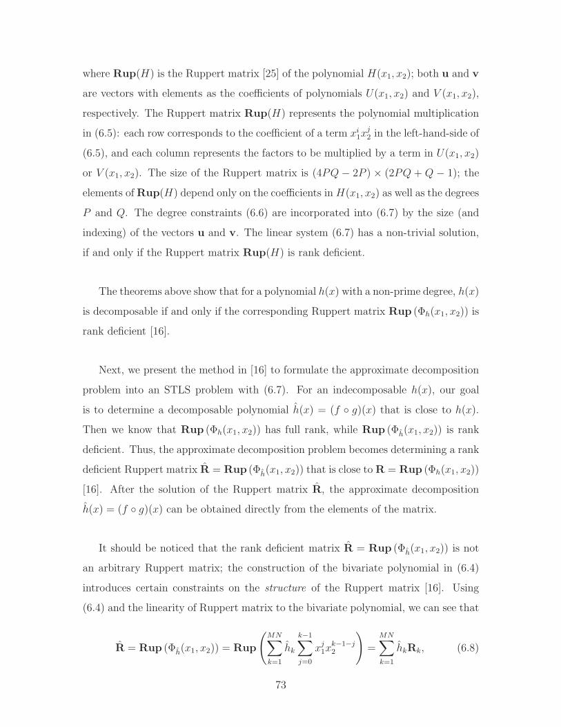
where Rup(H) is the Ruppert matrix [25] of the polynomial H(x1, x2); both u and v
are vectors with elements as the coefficients of polynomials U(x1, x2) and V (x1, x2),
respectively. The Ruppert matrix Rup(H) represents the polynomial multiplication
in (6.5): each row corresponds to the coefficient of a term xi1xj2 in the left-hand-side of
(6.5), and each column represents the factors to be multiplied by a term in U(x1, x2)
or V (x1, x2). The size of the Ruppert matrix is (4PQ − 2P ) × (2PQ + Q − 1); the
elements ofRup(H) depend only on the coefficients inH(x1, x2) as well as the degrees
P and Q. The degree constraints (6.6) are incorporated into (6.7) by the size (and
indexing) of the vectors u and v. The linear system (6.7) has a non-trivial solution,
if and only if the Ruppert matrix Rup(H) is rank deficient.
The theorems above show that for a polynomial h(x) with a non-prime degree, h(x)
is decomposable if and only if the corresponding Ruppert matrix Rup (Φh(x1, x2)) is
rank deficient [16].
Next, we present the method in [16] to formulate the approximate decomposition
problem into an STLS problem with (6.7). For an indecomposable h(x), our goal
is to determine a decomposable polynomial h(x) = (f ◦ g)(x) that is close to h(x).
Then we know that Rup (Φh(x1, x2)) has full rank, while Rup (Φh(x1, x2)) is rank
deficient. Thus, the approximate decomposition problem becomes determining a rank
deficient Ruppert matrix R = Rup (Φh(x1, x2)) that is close toR = Rup (Φh(x1, x2))
[16]. After the solution of the Ruppert matrix R, the approximate decomposition
h(x) = (f ◦ g)(x) can be obtained directly from the elements of the matrix.
It should be noticed that the rank deficient matrix R = Rup (Φh(x1, x2)) is not
an arbitrary Ruppert matrix; the construction of the bivariate polynomial in (6.4)
introduces certain constraints on the structure of the Ruppert matrix [16]. Using
(6.4) and the linearity of Ruppert matrix to the bivariate polynomial, we can see that
R = Rup (Φh(x1, x2)) = Rup
(MN∑
k=1
hk
k−1∑
j=0
xj1xk−1−j2
)=
MN∑
k=1
hkRk, (6.8)
73

where the matrices Rk are
Rk = Rup
(k−1∑
j=0
xj1xk−1−j2
), 1 ≤ k ≤MN. (6.9)
With the structure in (6.8), the approximate decomposition problem has been
transformed into the following optimization problem [16], which is an instance of the
Structured Total Least Square (STLS) problem [21, 24].
minh
‖h− h‖2, (6.10)
s. t. R =MN∑
k=1
hkRk is rank deficient. (6.11)
Finally, we turn to the solution of the STLS problem in (6.10). There is no exact
solution to the STLS problem, but there are heuristic algorithms [21–24, 26]. Here
we show two algorithms, namely a heuristic algorithm based on Riemannian singular
vector decomposition [21] and the STLS relaxation algorithm [22, 26]. We can note
that the constant term in h(x) does not influence its decomposability, so we only care
about the other terms in h(x) in the development of the following algorithms.
A Heuristic Based on Riemannian Singular Vector Decomposition
The problem in (6.10) is a special instance of the Riemannian Singular Vector De-
composition (RiSVD) framework [21], and the RiSVD problem can be solved by an
iterative heuristic algorithm proposed in [21].
The RiSVD formulation for the STLS problem in (6.10) aims to obtain vectors p,
q, and the smallest scalar τ such that
Rq = Dqpτ, (6.12)
RTp = Dpqτ, (6.13)
pTDqp = qTDpq = 1, (6.14)
74

where R is the Ruppert matrix, and the matrices Dp and Dq are
Dp =MN∑
k=1
RTkp(RT
kp)T, (6.15)
Dq =
MN∑
k=1
Rkq (Rkq)T . (6.16)
After the solution to the RiSVD problem, the approximate decomposition result
h(x) is obtained by:
hk = hk − pTRkqτ, k = 1, 2, . . . ,MN. (6.17)
Although there is no exact algorithm for the RiSVD problem, there is a heuristic
solution that is referred to as the inverse iteration algorithm [21, 24]. The algorithm
is described as follows.
Inverse Iteration Algorithm for the RiSVD Formulation [21, 24]
(1) Perform the QR decomposition of the matrix R, i.e., [C1 C2]
S
0
= R.
(2) Perform the SVD of the matrix R, and obtain the smallest singular
value τ (0) and the associated singular vectors p(0) and q(0).
(3) Compute γ(0) = ((q(0))TDp(0)q(0))14 .
(4) Normalize p(0) = p(0)
γ(0) , q(0) = q(0)
γ(0) .
(5) In the k-th iteration:
(6) Compute z(k) = (S−1)TDp(k−1)q(k−1)τ (k−1).
(7) Compute w(k) = −(CT2Dq(k−1)C2)
−1(CT2Dq(k−1)C1)z
(k).
(8) Compute p(k) = C1z(k) +C2w
(k).
(9) Compute q(k) = S−1CT1Dq(k−1)p(k).
(10) Normalize q(k) = q(k)
‖q(k)‖2.
(11) Compute γ(k) = ((q(k))TDp(k)q(k))14 .
(12) Renormalize p(k) = p(k)
γ(k) , q(k) = q(k)
γ(k) .
(13) Compute τ (k) = (p(k))TRq(k).
75

(14) Continue until the associated Ruppert matrix is numerically rank deficient
or k attains the limit on iteration steps.
(15) Obtain the final approximate decomposition result h(x) from (6.17).
STLS Relaxation
This algorithm is based on the algorithms in [22, 26]. It relaxes the constraint of
rank deficiency of the Ruppert matrix into a penalty term in the cost function. The
Ruppert matrix R in (6.11) is rank deficient if and only if one column is a linear
combination of the other columns. By switching two columns, we can always make
the last column linearly dependent on other columns. Then the problem of (6.10) is
equivalent to
minh,y
‖h− h‖2, (6.18)
s. t. R
y
−1
= 0, (6.19)
where the vector [yT,−1]T is in the null space of the matrix R. The constraint in
(6.19) is nonlinear with respect to the pair (h,y), since the matrix R depends on the
coefficients of h. A relaxation of (6.18) is [22, 26]
minh,y
C(h,y) , ‖h− h‖22 + λ
∥∥∥∥∥∥R
y
−1
∥∥∥∥∥∥
2
2
, (6.20)
where the parameter λ balances the deviation of polynomial h(x) from h(x) and the
energy of the residue vector R[yT,−1]T.
The choice of λ is important for the quality of the relaxation problem (6.20). On
one hand, if λ is large, the residue vector has low energy, but the polynomial h(x) may
not be a close approximation to h(x). On the other hand, if λ is small, the polynomial
h(x) may be near the original h(x), but the rank deficiency of the Ruppert matrix
may be significantly violated.
76
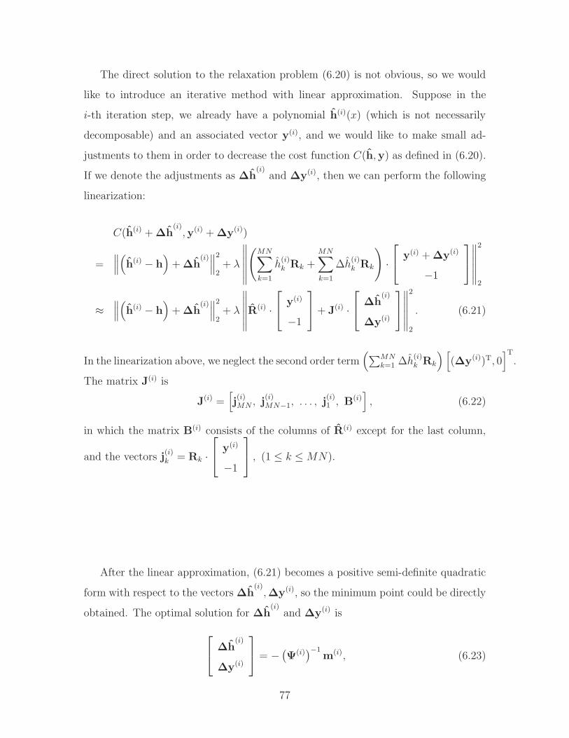
The direct solution to the relaxation problem (6.20) is not obvious, so we would
like to introduce an iterative method with linear approximation. Suppose in the
i-th iteration step, we already have a polynomial h(i)(x) (which is not necessarily
decomposable) and an associated vector y(i), and we would like to make small ad-
justments to them in order to decrease the cost function C(h,y) as defined in (6.20).
If we denote the adjustments as ∆h(i)
and ∆y(i), then we can perform the following
linearization:
C(h(i) +∆h(i),y(i) +∆y(i))
=∥∥∥(h(i) − h
)+∆h
(i)∥∥∥2
2+ λ
∥∥∥∥∥∥
(MN∑
k=1
h(i)k Rk +
MN∑
k=1
∆h(i)k Rk
)·
y(i) +∆y(i)
−1
∥∥∥∥∥∥
2
2
≈∥∥∥(h(i) − h
)+∆h
(i)∥∥∥2
2+ λ
∥∥∥∥∥∥R(i) ·
y(i)
−1
+ J(i) ·
∆h
(i)
∆y(i)
∥∥∥∥∥∥
2
2
. (6.21)
In the linearization above, we neglect the second order term(∑MN
k=1 ∆h(i)k Rk
) [(∆y(i))T, 0
]T.
The matrix J(i) is
J(i) =[j(i)MN , j
(i)MN−1, . . . , j
(i)1 , B
(i)], (6.22)
in which the matrix B(i) consists of the columns of R(i) except for the last column,
and the vectors j(i)k = Rk ·
y(i)
−1
, (1 ≤ k ≤MN).
After the linear approximation, (6.21) becomes a positive semi-definite quadratic
form with respect to the vectors ∆h(i),∆y(i), so the minimum point could be directly
obtained. The optimal solution for ∆h(i)
and ∆y(i) is
∆h
(i)
∆y(i)
= −
(Ψ(i)
)−1m(i), (6.23)
77
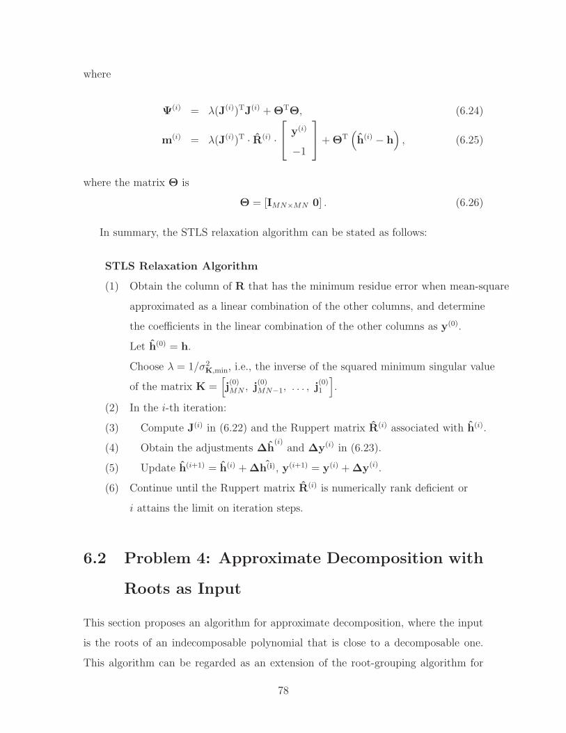
where
Ψ(i) = λ(J(i))TJ(i) +ΘTΘ, (6.24)
m(i) = λ(J(i))T · R(i) ·
y(i)
−1
+ΘT
(h(i) − h
), (6.25)
where the matrix Θ is
Θ = [IMN×MN 0] . (6.26)
In summary, the STLS relaxation algorithm can be stated as follows:
STLS Relaxation Algorithm
(1) Obtain the column of R that has the minimum residue error when mean-square
approximated as a linear combination of the other columns, and determine
the coefficients in the linear combination of the other columns as y(0).
Let h(0) = h.
Choose λ = 1/σ2K,min, i.e., the inverse of the squared minimum singular value
of the matrix K =[j(0)MN , j
(0)MN−1, . . . , j
(0)1
].
(2) In the i-th iteration:
(3) Compute J(i) in (6.22) and the Ruppert matrix R(i) associated with h(i).
(4) Obtain the adjustments ∆h(i)
and ∆y(i) in (6.23).
(5) Update h(i+1) = h(i) +∆h(i), y(i+1) = y(i) +∆y(i).
(6) Continue until the Ruppert matrix R(i) is numerically rank deficient or
i attains the limit on iteration steps.
6.2 Problem 4: Approximate Decomposition with
Roots as Input
This section proposes an algorithm for approximate decomposition, where the input
is the roots of an indecomposable polynomial that is close to a decomposable one.
This algorithm can be regarded as an extension of the root-grouping algorithm for
78

exact decomposition. Since the polynomial is indecomposable, the groups of roots
are actually not fully defined and not unique. However, if we view the roots of an
indecomposable polynomial as the roots of a decomposable polynomial with some
perturbation, then we may use the grouping information of the nearby decomposable
polynomial for decomposition.
The algorithm consists of iterations, in each of which there are three phases: the
first phase is to determine the grouping information using mixed integer programming;
the second phase is to determine whether to terminate the iteration by obtaining a
decomposable polynomial and measuring its approximation quality to the input poly-
nomial from the perspective of roots; the third phase is to make small adjustments to
the roots of an indecomposable polynomial to approach a decomposable polynomial.
Only the third phase updates the roots of the indecomposable polynomial; the roots
of a decomposable polynomial obtained in the second phase of an iteration are for
the only purpose of determining whether the termination criterion has been met, and
they are not used in the third phase or any future iterations; the reason for this is
explained in the description of the second phase.
In the first phase of each iteration, the grouping information is obtained with a
formulation of a mixed integer program, which is similar to that in the root-grouping
algorithm for exact decomposition. Since the roots are of an indecomposable polyno-
mial, the equality of the power summations (5.9) does not hold and can no longer be
directly applied to determine the grouping information; however, if the perturbation
is small, there should not be significant differences among the power summations of
the roots sj(Ai) in each group 1 ≤ i ≤ M for a given order 1 ≤ j ≤ N − 1, where
sj(Ai) is defined in (5.5). As a result, we consider the most likely grouping pattern
to be the one that minimizes the total difference among the power summations of the
roots in each group. In particular, we formulate a mixed integer program as follows:
79

minδk,i,sj ,εi,j
M∑
i=1
N−1∑
j=1
|εi,j| (6.27)
s. t. εi,j =
MN∑
k=1
δk,i · (zh(k))j − sj , for 1 ≤ i ≤M, 1 ≤ j ≤ N − 1, (6.28)
MN∑
k=1
δk,i = N, for 1 ≤ i ≤M, (6.29)
M∑
i=1
δk,i = 1, for 1 ≤ k ≤ MN, (6.30)
δk,i ∈ {0, 1}, for 1 ≤ k ≤MN, 1 ≤ i ≤ M.
This optimization problem has the following variables: binary variables δk,i that in-
dicate whether the root zh(k) belongs to the group Ai, continuous variables sj that
are the standard root power summation of order j, and continuous variables εi,j that
are the deviation from the root power summation of order j in the i-th group to the
corresponding standard root power summation sj. Since the roots zh(k) are mostly
complex numbers, the deviations εi,j are respectively implemented for the real part
and the imaginary part, and each term |εi,j| in the cost function (6.27) is imple-
mented as |εi,j| , |Re {εi,j}| + |Im {εi,j}|. For decomposable polynomials with real
coefficients, the standard root power summations sj always have real values due to
Newton’s identities [28]; thus, in our implementation, we constrain that sj are all real.
In this way, the formulation above is in the framework of mixed integer optimization.
The constraints (6.29) and (6.30) ensure that each group has N roots zh and that
each zh belongs to one group, respectively. The cost function is the total difference
between the power summations in each group and the corresponding standard power
summations.
The formulation above can obtain the correct grouping pattern if the perturbation
is small. If there is no perturbation, the formulation in (6.27) obtains the correct
grouping information with a minimum cost of zero, since all the differences in power
summations are zero due to Theorem 5.3. If the perturbation gradually increases from
80

zero but is sufficiently small, the differences of power summations εi,j also gradually
increase, and the correct grouping information δk,i still has lower cost to the problem
(6.27) than any incorrect grouping patterns; thus, the solution to (6.27) leads to the
true grouping pattern if the perturbation is sufficiently small. This conclusion does
not hold for the large perturbation scenario, where an incorrect grouping pattern may
achieve a lower cost than the correct one.
The formulation (6.27) for the approximate decomposition algorithm has higher
complexity than the formulation (5.8) for the exact decomposition algorithm. In the
exact decomposition algorithm, the grouping process can be divided into multi-steps,
each of which solves a mixed integer program and determines only one new group of
roots using Theorem 5.3. However, for the approximate decomposition algorithm, all
the groups are determined simultaneously in one step rather than multi-stages, since
Theorem 5.3 does not hold for the approximate case and the cost function in (6.27) is
globally dependent on all the groups. As a result, the dimension and the complexity
of the optimization problem increase for approximate decomposition.
In the second phase of each iteration, we obtain the roots of a decomposable
polynomial and determine whether to terminate the iteration. With the current
roots zh which typically do not correspond to a decomposable polynomial, we first
utilize the linear program in (5.13) to determine the roots zf and the coefficients of
g(x), and then we construct f(x) from zf . Last, by solving (3.7) with the obtained
zf and g(x), we reconstruct the zh as the roots of (f ◦ g)(x), which are guaranteed
to correspond to a decomposable polynomial. When the total deviation from the
perturbed input roots to the roots zh is sufficiently small, we consider the algorithm
as convergent and terminate the iterations; if not, we continue to the third phase
and the next iteration. We want to clarify that the roots zh in an iteration are not
used in the following third phase or in future iterations: although zh correspond to a
decomposable polynomial, however, zh may be significantly deviated from the input
roots due to the way they are obtained; in contrast, if we make small adjustments
on the roots zh of the indecomposable polynomial (in the following third phase) and
obtain a new set of zh from the adjusted roots (in the second phase of the next
81

iteration), it is possible that the new set of zh is closer to the input roots than the
previous set. Since we want to find a decomposable polynomial whose roots are good
approximation to the input roots, we do not use the roots zh as the starting point of
the adjustment in the third phase. As a result, we only update the roots zh in the
third phase, although zh typically do not correspond to a decomposable polynomial.
In the third phase of each iteration, we adjust the roots zh (not the roots zh
that are obtained in the second phase) with Taylor approximation to approach a
decomposable polynomial. We aim to approximately minimize the total difference of
power summations with proper adjustment of the roots. Specifically, if the roots zh(k)
are slightly adjusted by ∆zh(k), then the j-th power is adjusted by j (zh(k))j−1·∆zh(k)
to the first-order Taylor approximation. As a result, a linear program is formulated
as follows.
min∆zh(k),sj ,εi,j
M∑
i=1
N−1∑
j=1
|εi,j|+W ·
MN∑
k=1
|∆zh(k)| (6.31)
s. t. εi,j =MN∑
k∈Ai
((zh(k))
j + j (zh(k))j−1 ·∆zh(k)
)− sj ,
for 1 ≤ i ≤ M, 1 ≤ j ≤ N − 1. (6.32)
Similar with the first phase, sj and εi,j in (6.32) represent the standard power summa-
tions and the approximate deviations in power summations, respectively; in addition,
sj are constrained to have real values. The same as (6.28) in the first phase, εi,j in
the constraint (6.32) are implemented for the real part and imaginary part, respec-
tively, and in the cost function |εi,j| , |Re{εi,j}|+ |Im{εi,j}|. The groups Ai in (6.32)
are obtained from the results in the first phase, i.e., Ai = {k|δk,i = 1}. In the cost
function, W is a weight factor to balance between achieving a small total difference of
power summations and lowering down the adjustments of the roots. Since ∆zh(k) are
probably complex numbers, we implement |∆zh(k)| , |Re{∆zh(k)}|+ |Im{∆zh(k)}|.
In addition, we have two details for implementation: first, we constrain that the ad-
justments of conjugate roots are also conjugate to ensure that h(x) is a real-coefficient
polynomial after the adjustments of the roots; second, we set a upper bound for the
82

real and imaginary parts of each ∆zh(k) to avoid huge adjustments which may de-
crease the precision of the Taylor approximation. Since Taylor expansion is used in
(6.32), the adjusted roots from linear program in the third phase typically do not
correspond to a decomposable polynomial.
An iteration with the three phases above may approach a decomposable polynomi-
al. As we mentioned in the second phase, when the total deviation from the perturbed
input roots to the roots zh of the decomposable polynomial in the iteration is suf-
ficiently small, we consider the algorithm as convergent. However, we do not have
a guarantee for convergence or global optimality. The approximate decomposition
algorithm with roots as input is summarized as follows.
Approximate Root-Grouping Algorithm
(1) In the i-th iteration:
(2) Phase 1: Solve the mixed integer optimization (6.27).
(3) Phase 2: Solve (5.13) and obtain the coefficients g(i)(x) and the roots
z(i)f (k), (1 ≤ k ≤M). Then obtain f (i)(x) =
∏M
k=1
(x− z
(i)f (k)
).
Solve (3.7) to obtain the roots of the decomposable polynomial
(f (i) ◦ g(i))(x), denoted as zh(i)(k) (1 ≤ k ≤MN).
(4) Phase 3: Solve the linear optimization (6.31) to get ∆z(i)h (k).
Adjust the roots z(i)h (k) = z
(i−1)h (k) + ∆z
(i)h (k), for 1 ≤ k ≤ MN .
(5) Continue until the total deviation from the perturbed input roots to the
roots zh(i)(k) obtained in step (3) is sufficient small, or i attains the limit
on iteration steps.
6.3 Evaluation of the Approximate Decomposition
Algorithms
This section presents the evaluation of the four algorithms for approximate decom-
position. In the simulation, we vary the degrees of f(x) and g(x); for each degree
83
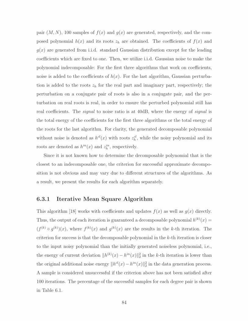
pair (M,N), 100 samples of f(x) and g(x) are generated, respectively, and the com-
posed polynomial h(x) and its roots zh are obtained. The coefficients of f(x) and
g(x) are generated from i.i.d. standard Gaussian distribution except for the leading
coefficients which are fixed to one. Then, we utilize i.i.d. Gaussian noise to make the
polynomial indecomposable: For the first three algorithms that work on coefficients,
noise is added to the coefficients of h(x). For the last algorithm, Gaussian perturba-
tion is added to the roots zh for the real part and imaginary part, respectively; the
perturbation on a conjugate pair of roots is also in a conjugate pair, and the per-
turbation on real roots is real, in order to ensure the perturbed polynomial still has
real coefficients. The signal to noise ratio is at 40dB, where the energy of signal is
the total energy of the coefficients for the first three algorithms or the total energy of
the roots for the last algorithm. For clarity, the generated decomposable polynomial
without noise is denoted as hcl(x) with roots zclh , while the noisy polynomial and its
roots are denoted as hin(x) and zinh , respectively.
Since it is not known how to determine the decomposable polynomial that is the
closest to an indecomposable one, the criterion for successful approximate decompo-
sition is not obvious and may vary due to different structures of the algorithms. As
a result, we present the results for each algorithm separately.
6.3.1 Iterative Mean Square Algorithm
This algorithm [18] works with coefficients and updates f(x) as well as g(x) directly.
Thus, the output of each iteration is guaranteed a decomposable polynomial h(k)(x) =
(f (k) ◦ g(k))(x), where f (k)(x) and g(k)(x) are the results in the k-th iteration. The
criterion for success is that the decomposable polynomial in the k-th iteration is closer
to the input noisy polynomial than the initially generated noiseless polynomial, i.e.,
the energy of current deviation ‖h(k)(x)− hin(x)‖22 in the k-th iteration is lower than
the original additional noise energy ‖hcl(x)−hin(x)‖22 in the data generation process.
A sample is considered unsuccessful if the criterion above has not been satisfied after
100 iterations. The percentage of the successful samples for each degree pair is shown
in Table 6.1.
84

Table 6.1: Success Rate of the Iterative Mean Square Algorithm (%)
deg(f) deg(g) deg(f ◦ g) Success Rate
2 2 4 100.03 3 9 100.03 4 12 98.04 4 16 94.04 5 20 84.05 5 25 67.05 6 30 37.06 6 36 26.06 7 42 12.07 7 49 12.0
The iterative mean square algorithm achieves success in all but 2 samples with
degrees below 12 in our simulation. For higher degrees, it has unsuccessful samples,
either because the algorithm diverges or it converges to a local minimum. In conclu-
sion, the iterative mean square algorithm is a practical and efficient approach if the
input polynomial is close to a decomposable polynomial and its degree is not high,
although there is no guarantee of the convergence to the global minimum.
6.3.2 RiSVD Heuristic and STLS Relaxation
The goal of both RiSVD and STLS relaxation algorithms is to determine a rank
deficient Ruppert matrix that is close to the full rank initial Ruppert matrix. Thus,
these algorithms are considered successful when the Ruppert matrix is numerically
rank deficient, which is determined by the singular values in our simulation. In
particular, a Ruppert matrix is considered rank deficient if the maximum gap between
consecutive singular values among the smallest 20 singular values is larger than 100
times that of the initial Ruppert matrix or larger than 104. A sample is considered
unsuccessful if the criterion above has not been satisfied after 100 iterations. The
success rates of the RiSVD and STLS algorithms are listed in Table 6.2.
In Table 6.2, the success rate is the ratio between total successful samples and the
number of samples where the initial Ruppert matrix is not numerically rank deficient
85

Table 6.2: Success Rate of the Approximate Decomposition Methods that are Basedon Ruppert Matrix (%)
deg(f) deg(g) deg(f ◦ g) RiSVD STLN
2 2 4 73.0 100.02 3 6 2.0 97.03 2 6 9.0 96.02 4 8 5.0 92.04 2 8 7.3 94.83 3 9 5.0 86.02 5 10 1.0 81.05 2 10 10.0 90.02 6 12 2.0 79.03 4 12 12.2 83.74 3 12 10.0 82.26 2 12 11.3 95.0
(i.e., the maximum gap between consecutive singular values among the smallest 20
singular values is smaller than 104 for the initial matrix). The success rate of the
STLS relaxation algorithm is higher than that of the RiSVD algorithm, which shows
the STLS algorithm performs better in generating numerically rank deficient Ruppert
matrices.
However, complications involving numerical accuracy are encountered for these
two algorithms. In contrast to the iterative mean square method [18] and the approx-
imate root-grouping decomposition method where the polynomial in each iteration
is guaranteed decomposable, the polynomial corresponding to the Ruppert matrix
in each iteration of RiSVD and SLTS algorithms is generally indecomposable. Even
if both RiSVD and STLS converge under our criterion of numerical rank deficiency,
the output polynomials of the RiSVD or STLS algorithms are possibly unable to be
faithfully decomposed with the coefficient-unraveling algorithm for exact decomposi-
tion [17]. In addition, the polynomials obtained by RiSVD may have better perfor-
mance than those by STLS, when they are decomposed by the coefficient-unraveling
algorithm. This implies that our criterion for rank deficiency is not necessarily com-
patible with the coefficient-unraveling algorithm. Although rank deficiency of Rup-
86

pert matrix is theoretically equivalent to decomposability of polynomial, the large
dimensions of Ruppert matrices may cause numerical errors that lead to imprecision
in the singular value calculation in MATLAB, so our rank deficient criterion may not
be determined precisely.
6.3.3 Approximate Root-Grouping Algorithm
This section presents the simulation results for the approximate root-grouping algo-
rithm. In the data generation process, perturbation with 40dB SNR is added to the
roots of decomposable polynomials; the perturbation on a conjugate pair of roots
is also in a conjugate pair, and the perturbation on real roots is real, so the per-
turbed polynomial still has real coefficients. The weight factor in (6.31) is chosen as
W = 10−2, and we set an upper bound of 10−3 for the real and imaginary parts of each
adjustment ∆zh(k) in the third phase of each iteration. As we discussed in Section
6.2, the output zh in the second phase of each iteration is guaranteed to correspond to
a decomposable polynomial. Consequently, we choose the criterion for success as that
the roots zh of the decomposable polynomial in the k-th iteration are closer to the
perturbed input roots than the roots of the initially generated decomposable polyno-
mial are; in other words, we find a better decomposable approximation to the input
polynomial than the original one in the data generation process, from the perspective
of the energy of the differences of roots. A sample is considered unsuccessful if the
criterion above has not been satisfied after 100 iterations. The successful percentage
for each degree pair is shown in Table 6.3.
In Table 6.3, the column of correct grouping information shows the results for the
first phase of the algorithm, which determines the grouping information; the column
of successful decomposition shows the percentage of the successful samples according
to the criterion above. If h(x) has a degree that is below 20, the approximate root-
grouping algorithm in our simulation achieves considerable success. All grouping
information is correctly obtained when the degree of the polynomial h(x) is below 12;
as the degree increases, there are cases where the grouping information is not correctly
determined; since the total number of possible grouping patterns increases with the
87
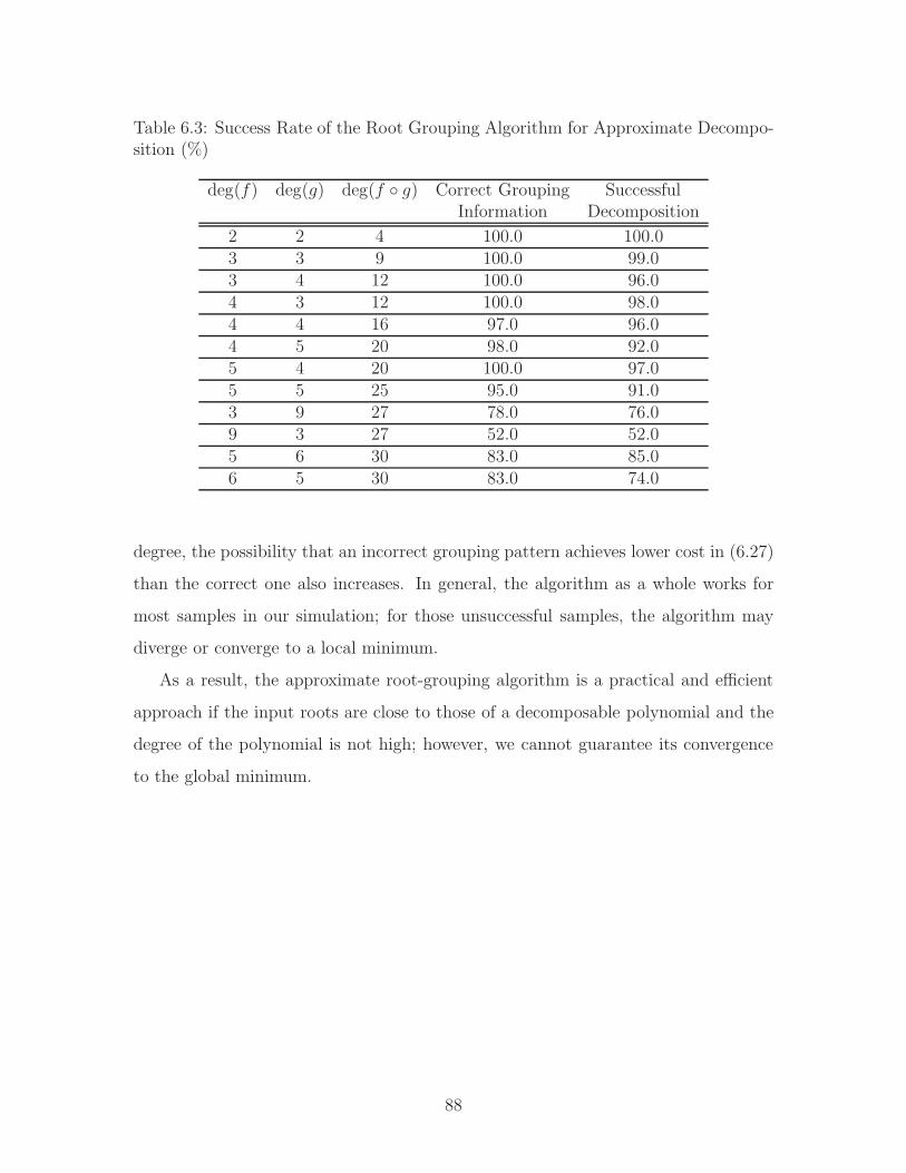
Table 6.3: Success Rate of the Root Grouping Algorithm for Approximate Decompo-sition (%)
deg(f) deg(g) deg(f ◦ g) Correct Grouping SuccessfulInformation Decomposition
2 2 4 100.0 100.03 3 9 100.0 99.03 4 12 100.0 96.04 3 12 100.0 98.04 4 16 97.0 96.04 5 20 98.0 92.05 4 20 100.0 97.05 5 25 95.0 91.03 9 27 78.0 76.09 3 27 52.0 52.05 6 30 83.0 85.06 5 30 83.0 74.0
degree, the possibility that an incorrect grouping pattern achieves lower cost in (6.27)
than the correct one also increases. In general, the algorithm as a whole works for
most samples in our simulation; for those unsuccessful samples, the algorithm may
diverge or converge to a local minimum.
As a result, the approximate root-grouping algorithm is a practical and efficient
approach if the input roots are close to those of a decomposable polynomial and the
degree of the polynomial is not high; however, we cannot guarantee its convergence
to the global minimum.
88

Chapter 7
Conclusions and Future Work
This thesis studies the sensitivities of polynomial composition and decomposition in
order to characterize their robustness with respect to perturbations in coefficients
and roots. It also presents algorithms for both exact and approximate polynomial
decomposition. Since both the coefficients and the roots of decomposable polyno-
mials are potentially useful in signal processing applications, we explore polynomial
decomposition with inputs of both coefficients and roots.
For sensitivity analysis, we have derived the expressions and developed bounds for
the sensitivities. An empirical comparison shows that composition and decomposition
using the root triplet (zf , g, zh) is likely to be more robust than using the coefficient
triplet (f, g, h), when the degrees of polynomials are sufficiently high. Simulation
results demonstrate that the sensitivities Sf→h and Sh→f can be significantly reduced
by utilizing equivalent compositions with first-degree polynomials; in addition, our
heuristic rule for parameter selection is shown to be efficient in approaching the
minimum values for these sensitivities.
Three algorithms are presented for the exact decomposition problem, in which
the polynomial h(x) is ensured to be decomposable into polynomials with specified
degrees. These algorithms all work in theory but have different numerical perfor-
mances. Simulation results show that the algorithms with roots as input are more
robust to numerical errors and can decompose polynomials with much higher degrees
than the algorithm with coefficients as input. Specifically, the root-power-summation
89
algorithm has the highest successful decomposition rate; the root-grouping algorithm
has a step of mixed integer programming, which may have high complexity but is
empirically shown much more efficient than general integer programming problem-
s; the coefficient-unraveling algorithm does not use all the coefficients of the input
polynomial in the step to get g(x) and easily accumulates numerical error due to its
structure.
Four algorithms are shown for the approximate decomposition problem, for which
we want to approximate h(x) with a decomposable polynomial. Three algorithms
work with coefficients: one is an iterative mean square method, and the other two
are based on obtaining a rank deficient Ruppert matrix that approximates that of
the indecomposable polynomial. The fourth algorithm has roots as input. Although
each algorithm may be effective for certain polynomials, none of these algorithms is
guaranteed to converge in general settings. The iterative mean square method is a
practical and efficient algorithm if the input polynomial is near a decomposable one,
but it may converge into a local minimum. The algorithms based on the Ruppert
matrix may obtain a numerically rank deficient Ruppert matrix, but they encounter
numerical problems in computation with the high-dimension Ruppert matrix and in
the determination of the rank, so the output polynomials of these algorithms are
possibly unable to be faithfully decomposed with the coefficient-unraveling algorithm
for exact decomposition; in addition, the choice for an parameter in SLTS algorithm is
not clear. The approximate root-grouping algorithm is effective when the input roots
are near those of a decomposable polynomial, but it may also converge to a local
minimum and the optimal values of parameters in this algorithm are not obvious.
Future work would mainly focus on further development and improvement of the
approximate decomposition algorithms. For these existing algorithms, the conver-
gence criteria may be derived to understand the conditions under which the algo-
rithms converge to the globally optimal decomposable approximation. In addition,
accurate numerical methods to determine the rank of a high-dimension matrix may
improve the termination criteria of the RiSVD and the STLS algorithms as well as
enable these algorithms to work on polynomials with higher degrees. With potential
90

improvements on numerical accuracy, efficient criteria for comparison among algo-
rithms also need to be developed and verified.
New algorithms could also be developed with potentially deeper exploration in
theory or practice. As an example in theory, the RiSVD and STLS algorithms are
both for the general STLS problem but do not make full use of the special structure
of the Ruppert matrix; thus, further study on the structure of the Ruppert matrix
may lead to invention of algorithms with higher efficiency. In practice, exploration
of the properties of the signals to be approximately decomposed may constrain the
range of the problem and result in more specific but more efficient algorithms.
In addition to algorithms, tighter lower bounds may be developed on the dis-
tance from an indecomposable polynomial to its nearest decomposable approxima-
tion, which may serve as a fundamental limit and be used to evaluate the room for
improvement of approximate decomposition algorithms.
91

92

Appendix A
Minimum Phase Decomposition for
a Minimum Phase Decomposable
Polynomial
In this appendix, we proof the statement in Item 6 in Section 2.1: if a decomposable
h(x) is minimum phase, then there always exists a non-trivial minimum phase decom-
position. In other words, if we know that a minimum phase h(x) has the composition
h(x) = (f ◦ g)(x), (A.1)
where deg(f(x)) =M and deg(g(x)) = N (M > 1 and N > 1), then we can construct
an equivalent composition of h(x) into minimum phase components f(x) and g(x)
with degrees M and N , respectively. Here minimum phase polynomials refer to the
polynomials the roots of which are all inside the unit circle. We assume f(x), g(x)
and h(x) are all real polynomials, and we require that both f(x) and g(x) have only
real coefficients.
Since minimum phase depends on the radius of the roots, we first study the
structure of the roots of a decomposable polynomial.1 If we denote the roots of f(x)
1Similar discussion about the structure of roots of a decomposable polynomial is also presentedin Section 4.1.2.
93

and h(x) as zf (i) (1 ≤ i ≤M) and zh(k) (1 ≤ k ≤MN), respectively, then there are
two ways to factor the composed polynomial h(x):
h(x) = aM
M∏
i=1
(g(x)− zf (i)) = cMN
MN∏
k=1
(x− zh(k)) . (A.2)
where aM and cMN are the coefficients of the highest degree term in f(x) and h(x),
respectively. Denote
g1(x) , g(x)− zf(1), (A.3)
then (A.2) implies that all the roots of g1(x) are included in the roots of h(x). Since
h(x) is minimum phase, all its roots are in the unit circle, so all the roots of g1(x) are
in the unit circle. If zf (1) is a real number, then g1(x) is a real-coefficient polynomial;
otherwise, g1(x) has a complex constant term. We consider the following two cases,
which depend on whether f(x) has at least a real root.
Case 1: f(x) has at least a real root.
Without loss of generality, we can assume zf (1) is a real root of f(x). Then (A.2)
becomes
h(x) = aM
M∏
i=1
(g1(x)− (zf (i)− zf (1))) = (f1 ◦ g1)(x), (A.4)
where
f1(x) = aM
M∏
i=1
(x− (zf(i)− zf (1))) . (A.5)
The complex roots among zf (i) are in conjugate pairs since f(x) is real; in addition,
since zf(1) is real, we know the complex roots in (A.5) are also in conjugate pairs, so
f1(x) is a real polynomial.
The polynomial f1(x) is not necessarily minimum phase; however, we can con-
struct a minimum phase polynomial f(x) by scaling the roots:
f(x) = aM · θM1 ·
M∏
i=1
(x−
zf (i)− zf (1)
θ1
), (A.6)
94
where
θ1 = 2 · max1≤i≤N
|zf(i)− zf (1)|. (A.7)
The roots of f(x) are zf (i) =zf (i)−zf (1)
θ1, and we can verify that these roots have radius
|zf(i)| ≤max1≤i≤N |zf(i)− zf (1)|
θ1=
1
2.
Thus, all the roots of f(x) are in the unit circle, and f(x) is a minimum phase
polynomial. In addition, f(x) is a real polynomial since its complex roots are in
conjugate pairs.
To compensate the scaling in f(x), we need to scale g1(x) into g(x) correspond-
ingly:
g(x) =1
θ1· g1(x) =
1
θ1(g(x)− zf (1)) . (A.8)
Since g(x) has the same roots as g1(x) and g1(x) is minimum phase, we know g(x) is
also minimum phase. Since g1(x) is real, we know g(x) has also real coefficients.
The composition (f ◦ g)(x) yields
(f ◦ g)(x) = aM · θM1 ·M∏
i=1
(g(x)−
zf(i)− zf (1)
θ1
)
= aM ·M∏
i=1
(g(x)− zf (i))
= h(x). (A.9)
Thus, (f ◦ g)(x) is an equivalent composition of h(x), and both f(x) and g(x) are
minimum phase and real polynomials. This completes our proof for the first case
where f(x) has at least a real root.
Case 2: f(x) has only complex conjugate roots.
If f(x) has only complex roots in conjugate pairs, we know g1(x) = g(x)− zf (1) and
g∗1(x) = g(x)−z∗f (1) are both complex-coefficient minimum phase polynomials. Then,
95
we have the following lemma:
Lemma A.1. Let η(z) =∑N
i=0 ηizi be a real-coefficient polynomial with degree N . If
both (η(z) + jα) and (η(z)− jα) are minimum phase polynomials for a real number
α > 0, then η(z) is also minimum phase.
Proof. First, we show that if |γ| ≥ 1 +∑N
i=0 |ηi|, then (η(z)− jγ) has no root in the
unit circle. This can be shown by
|η(z)− jγ| ≥ |γ| − |η(z)| ≥ |γ| −N∑
i=0
|ηi| ≥ 1 6= 0,
for any complex number z in the unit circle.
Next, we show the curve ζ = {u ∈ C|u = η(z), |z| = 1} has at most 2N inter-
sections with the imaginary axis on the complex plane. Intuitively, the curve ζ is the
image of the unit circle when it is mapped by the polynomial η(z). For any intersec-
tion of ζ and the imaginary axis, we have Re{η(z)} = 0 for some z on the unit circle
(i.e., |z| = 1); this is equivalent to η(z) + η∗(z) = 0 for some z with |z| = 1. Since
η(z) has real coefficients, for any z on the unit circle, we have η∗(z) = η(z∗) = η(1/z).
Thus, the corresponding values of z of all the intersections of ζ and the imaginary
axis satisfy η(z) + η(1/z) = 0, which can be arranged into a polynomial of z with the
degree of 2N . Thus, the number of such intersections does not exceed 2N (since we
additionally require |z| = 1).
Finally, we show the relationship between the curve ζ on the complex plane and
the number of roots of (η(z)−jγ) that are inside the unit circle. Obviously, (η(z)−jγ)
has root(s) on the unit circle if and only if jγ is on the curve ζ . Thus, as γ varies,
the roots of (η(z)− jγ) move continuously, and the number of roots in the unit circle
changes by one each time when jγ crosses the curve ζ (including multiplicity). Since
(η(z)− jα) are minimum phase, it has all N roots in the unit circle; let γ moves from
α to 1 + max{α,∑N
i=0 |ηi|}, then jγ crosses the curve ζ for at least N times, since
the number of roots of (η(z)− jγ) that are in the unit circle decreases from N to 0.
Similarly, let γ moves from −α to −1−max{α,∑N
i=0 |ηi|}, then jγ crosses the curve
96

ζ for at least another N times. Since there are at most 2N intersections of ζ and
the imaginary axis jγ, there is no intersection between −α and α. So the number
of roots in the unit circle does not vary as γ changes from −α to α, i.e., all roots of
(η(z)− jγ) are in the unit circle for −α ≤ γ ≤ α. Specially, when γ = 0, η(z) has all
roots in the unit circle and thus is minimum phase.
This accomplishes the proof for Lemma A.1.
With the lemma above, we may construct a minimum phase polynomial g2(x):
g2(x) = g(x)− Re{zf(1)}. (A.10)
Since g2(x) has real-coefficients, we may construct f(x) and g(x) in a way similar to
case 1:
f(x) = aM · θM2 ·M∏
i=1
(x−
zf (i)− Re{zf(1)}
θ2
), (A.11)
g(x) =1
θ2(g(x)− Re{zf (1)}) , (A.12)
where the scaling factor is
θ2 = 2 · max1≤i≤N
|zf(i)− Re{zf (1)}|. (A.13)
In similar procedures with case 1, we may verify that both f(x) and g(x) are
minimum phase and real polynomials, and their composition (f ◦ g)(x) yields h(x).
This completes our proof for the second case where f(x) has only complex conjugate
roots.
Combining cases 1 and 2, we have proved the statement about the existence of
minimum phase decomposition for minimum phase decomposable polynomials.
97

98
Appendix B
Derivation of Upper Bound (4.13)
In this appendix, we derive the upper bound (4.13) for the sensitivity Sg→h. First,
we show the relationship between the polynomials d(x) and h(x). The definition of
the polynomial d(x) in (4.9) implies
d = G ·
0
MaM
(M − 1)aM−1
...
a1
= GVf = GVG†h, (B.1)
where the last step uses (5.3); G and V are defined in (4.2) and (4.15), respectively;
G† = (GTG)−1GT is the pseudo-inverse matrix of G.
Next, we want to bound the energy of ∆h(x) with the energy of ∆g(x). Since
(4.8) indicates ∆h(x) is approximately the convolution of ∆g(x) and d(x), we want to
bound the energy of the output signal with the two input signals of the convolution.
In general, we have the following lemma on the energy of the signals in a convolution.
Lemma B.1. Denote s3[n] as the convolution of the finite length signals s1[n] that is
non-zero only for 0 ≤ n ≤ L1 and s2[n] that is non-zero only for 0 ≤ n ≤ L2. Assume
L1 ≥ L2, then the energy of these signals satisfy
Es3 ≤ (L2 + 1)Es1Es2 , (B.2)
99

where the energy is given by Esi =∑∞
n=−∞ s2i [n], i = 1, 2, 3.
Proof. For 0 ≤ n ≤ L1 + L2, Cauchy-Schwarz inequality implies that
s23[n] =
min(L1,n)∑
m=max(0,n−L2)
s1[m]s2[n−m]
2
≤
min(L1,n)∑
m=max(0,n−L2)
s21[m]
min(L1,n)∑
m=max(0,n−L2)
s22[n−m]
≤
min(L1,n)∑
m=max(0,n−L2)
s21[m]
Es2.
Summing for n = 0, 1, . . . , (L1 + L2), we have
Es3 ≤
L1+L2∑
n=0
min(L1,n)∑
m=max(0,n−L2)
s21[m]
Es2 =
L1∑
m=0
(m+L2∑
n=m
s21[m]
)Es2 = (L2 + 1)Es1Es2 .
This accomplishes the proof for Lemma B.1.
Applying Lemma B.1 to (4.8), we know
E∆h ≤ (N + 1)E∆gEd, (B.3)
where E denotes the energy of the signals. A combination of (3.3) and (B.3) shows
Sg→h =‖g‖22‖h‖22
·max∆g
(‖∆h‖22‖∆g‖22
)≤
‖g‖22‖h‖22
· (N + 1)‖d‖22, (B.4)
where ∆g is a sufficiently small perturbation. Incorporating (B.1) into (B.4), we have
Sg→h ≤‖g‖22‖h‖22
· (N + 1)‖GVG†h‖22 ≤ (N + 1)‖g‖22 · σ2T,max, (B.5)
where T = GVG† = GV(GTG)−1GT is the matrix in (4.14), and σT,max is its
maximum singular value. Thus, we have completed the proof for (4.13).
100

Appendix C
Explanation of the Approximate
Rules (4.39)-(4.41) for Parameter
Selection
In this appendix, we develop the approximate rules (4.39)-(4.41) for parameter se-
lection for the first-degree polynomials in Section 4.2. In order to decrease the sen-
sitivities between the coefficients of f(x) and h(x), the rules propose values for the
parameters in the first-degree polynomial q(x) = q1x+ q0 to approximately minimize
the condition number of the associated matrix G in (4.34). In addition, we show the
function ‖(g(x) + qr)M‖22 in (4.39) is convex towards qr, so its minimum point can
be obtained efficiently. Moreover, we analyze the limit of the approximately optimal
parameters when M approaches infinity.
Before developing the rules, we first show a simple fact about the condition num-
ber. The condition number is the ratio between the maximum and the minimum
magnification of vector norm. Thus, for arbitrary vectors f1 and f2 that have dimen-
sion M + 1, the condition number satisfies
cond(G) =max
f(‖Gf‖2/‖f‖2)
minf(‖Gf‖2/‖f‖2)
≥‖Gf1‖2/‖f1‖2
‖Gf2‖2/‖f2‖2. (C.1)
101

As a result, the right-hand-side of (C.1) with any vectors f1 and f2 can serve as a
lower bound to the condition number.
The approximate rules will be explained with certain choices of f1 and f2 in (C.1).
For simplicity, we use an alternative expression of the first-degree polynomial q(x) =
q1(x+ qr), where qr =q0q1. We first show how to select qr with a fixed q1, and then we
consider a reasonable choice of q1.
Now we show reasons for the rule (4.39) for qr, when q1 is fixed. If we let f1 =
[1, 0, . . . , 0]T and f2 = [0, . . . , 0, 1]T, then (C.1) implies
cond(G) ≥ |q1|M · ‖(g(x) + qr)
M‖2. (C.2)
When q1 is fixed, the qr to minimize the right hand side in (C.2) is given by
qr = argminqr
‖(g(x) + qr)M‖2, (C.3)
which is equivalent to the rule in (4.39).
Then, we consider how to select q1, when qr is chosen according to (C.3). Denote
ei (0 ≤ i ≤ M) as the vector with 1 in the i-th element and 0 in the other elements.
By sweeping both of f1 and f2 over every ei (0 ≤ i ≤M), we may know
cond(G) ≥maxi=0,1,...,M |q1|
i · ‖(g(x) + qr)i‖2
mini=0,1,...,M |q1|i · ‖(g(x) + qr)i‖2, R(q1). (C.4)
The right-hand-side of (C.4) is a function of q1, which is denoted as R(q1). In fac-
t, R2(q1) is the ratio between the maximum and minimum energy among the self-
convolutions of g(x) = (q ◦ g)(x) up to M-th degree, so the minimization of R(q1)
aims to minimize the energy variation among the self-convolutions. We claim that
R(q1) is minimized when the energy of the polynomial (g(x))M equals 1, i.e.,
q1 =(‖(g(x) + qr)
M‖22)− 1
2M , (C.5)
which is the rule in (4.40).
102
To justify the claim in (C.5), we first demonstrate the energy of self-convolutions
E(i) = ‖(g(x))i‖22 (i = 0, 1, . . . ,M) is a convex function towards i with a fixed
g(x). For the length-(N + 1) signal b0, b1, . . . , bN where bi is the coefficient of the
term xi in g(x), we can zero-pad it and obtain its (MN + 1)-points Discrete Fourier
Transform (DFT) [4], which is denoted as G[k] (k = 0, 1, . . . ,MN). The convolution
theorem [4] implies that the DFT of the self-convolution (g(x))i (i ≤M) is Gi[k] (k =
0, 1, . . . ,MN), since the degree of (g(x))i (i ≤ M) does not exceed MN . As shown
by the Parseval’s theorem [4], the energy of self-convolution satisfies
E(i) = ‖(g(x))i‖22 =1
MN + 1
MN∑
k=0
|Gi[k]|2 =1
MN + 1
MN∑
k=0
|G[k]|2i, i = 0, 1, . . . ,M.
(C.6)
Since each term |G[k]|2i is convex with respect to i, the summation E(i) is a convex
function of i with any fixed polynomial g(x).
Then, we will show the function R(q1) decreases with q1 when 0 < q1 < q1, and it
increases with q1 when q1 > q1, which proves the claim that q1 is the minimum point
for R(q1). When 0 < q1 < q1, we know the energy E(M) = ‖(q1(g(x) + qr))M‖22 < 1;
since E(0) = 1 always holds, the convexity of E(i) implies E(i) < 1 = E(0) for
i = 1, 2, . . . ,M . As a result, the square of R(q1) becomes
R2(q1) =max
i=0,1,...,ME(i)
mini=0,1,...,M
E(i)=
1
E(m∗)=
1
‖(g(x) + qr)m∗‖22
· q−2m∗
1 ,
where m∗ = arg mini=1,...,M
E(i). Thus, R2(q1) is monotonically decreasing with q1 when
0 < q1 < q1. When q1 > q1, we know E(M) > 1 = E(0), so E(i) < E(M) for
i = 0, 1, . . . ,M − 1. Thus,
R2(q1) =max
i=0,1,...,ME(i)
mini=0,1,...,M
E(i)=E(M)
E(m∗)=
‖(g(x) + qr)M‖22
‖(g(x) + qr)m∗‖22
· q2(M−m∗)1 ,
where m∗ = arg mini=0,...,M−1
E(i). Thus, it is shown R2(q1) is monotonically increasing
with q1 when q1 > q1. This analysis completes the proof for the claim that q1 in (C.5)
103

is the optimal value to minimize R(q1) in (C.4).
At this point, we have shown the reasons for the approximate rules (4.39)-(4.41)
for the parameters of the first-degree polynomial.
Next, we show the function ‖(g(x)+qr)M‖22 is convex towards qr, which guarantees
the efficiency of obtaining qr in (4.39). If we let g(x) = g(x)+qr in the above analysis
of energy with DFT, then (C.6) becomes
‖(g(x) + qr)M‖22 =
1
MN + 1
MN∑
k=0
|G[k] + qr|2M ,
where G[k] is the (MN + 1)-point DFT of the coefficients of g(x). It can be verified
that the second derivative of each term |G[k] + qr|2M towards qr is non-negative, so
the summation is a convex function of qr. As a result, we may obtain qr in (4.39)
efficiently due to the convexity of ‖(g(x) + qr)M‖22.
Finally, we analyze the behaviors of qr and q1 in the limit scenario where M
approaches infinity. For g(x) =∑N
n=0 bnxn, the discrete-time Fourier transform [4] of
the sequence b0, b1, . . . , bN is g(e−jω) =∑N
n=0 bne−jnω. By the convolution theorem
and Parseval’s theorem [4], we can know the energy of the self-convolution (g(x)+qr)M
is
‖(g(x) + qr)M‖22 =
1
2π
∫ π
−π
|g(e−jω) + qr|2Mdω.
Thus, the rule for qr in (4.39) becomes
qr = argminqr
‖(g(x)+qr)M‖22 = argmin
qr
1
2π
∫ π
−π
|g(e−jω)+qr|2Mdω = argmin
qr‖g(e−jω)+qr‖2M ,
(C.7)
where ‖F (ω)‖2M =(∫ π
−π|F (ω)|2Mdω
) 12M
denotes the 2M-norm of a function on
the interval [−π, π]. As M → ∞, we know ‖F (ω)‖2M approaches the infinity-norm
‖F (ω)‖∞ = maxω |F (ω)|. Hence, the rule for qr has the following limit as M ap-
proaches infinity
qr → argminqr
(maxω
|g(e−jω) + qr|). (C.8)
104
Similar to the derivation above, the rule for q1 in (4.40) is equivalent to
q1 =
(1
2π
∫ π
−π
|g(e−jω) + qr|2Mdω
)− 12M
=
(1
2π
)− 12M
·(‖g(e−jω) + qr‖2M
)−1. (C.9)
When M approaches infinity, q1 has the limit
q1 →(max
ω|g(e−jω) + qr|
)−1
. (C.10)
An intuitive explanation of the results in the limit scenario is: the term qr smoothes
the spectrum of (q ◦ g)(e−jω) since it reduces the maximum peak, and the term q1
normalizes the peak of the spectrum in order to avoid significant expansion or shrink
of the energy of the self-convolutions with the increase of the degree M .
In addition, the limit scenario analysis implies: when the order of f(x) is sufficient-
ly large, we may also use the results in (C.8) and (C.10) to construct a first-degree
polynomial to efficiently reduce the condition number cond(G) as well as the sensitiv-
ities Sf→h and Sh→f . In addition, the evaluation of (C.8) and (C.10) does not depend
on M ; thus, compared with the rules (4.39) and (4.40), they may be more compu-
tationally efficient if the value of M may vary, at the expense of potentially lower
approximation quality to the optimal first-degree polynomial that actually minimizes
the condition number.
105

106

Bibliography
[1] D. Wei and A. V. Oppenheim, “Sampling based on local bandwidth,” in Signals,Systems and Computers (ASILOMAR), 2007 Conference Record of the FortyFirst Asilomar Conference on, 2007, pp. 1103–1107.
[2] D. Wei, “Sampling based on local bandwidth,” Master’s thesis, MassachusettsInstitute of Technology, 2007.
[3] J. Clark, M. Palmer, and P. Lawrence, “A transformation method for the recon-struction of functions from nonuniformly spaced samples,” Acoustics, Speech andSignal Processing, IEEE Transactions on, vol. 33, no. 5, pp. 1151–1165, 1985.
[4] A. V. Oppenheim and R. W. Schafer, Discrete-Time Signal Processing, 3rd ed.Upper Saddle River, NJ, USA: Prentice Hall Press, 2010.
[5] M. Blanco and F. Hill Jr, “On time warping and the random delay channel,”Information Theory, IEEE Transactions on, vol. 25, no. 2, pp. 155–166, 1979.
[6] R. Lummis, “Speaker verification by computer using speech intensity for tem-poral registration,” Audio and Electroacoustics, IEEE Transactions on, vol. 21,no. 2, pp. 80–89, 1973.
[7] S. Demirtas, “Functional composition and decomposition in signal processing,”Ph. D. Thesis Proposal, Massachusetts Institute of Technology, 2012.
[8] J. Kaiser and R. Hamming, “Sharpening the response of a symmetric nonre-cursive filter by multiple use of the same filter,” Acoustics, Speech and SignalProcessing, IEEE Transactions on, vol. 25, no. 5, pp. 415–422, 1977.
[9] T. Saramaki, “Design of fir filters as a tapped cascaded interconnection of iden-tical subfilters,” Circuits and Systems, IEEE Transactions on, vol. 34, no. 9, pp.1011–1029, 1987.
[10] S. Demirtas, G. Su, and A. V. Oppenheim, “Sensitivity of polynomial composi-tion and decomposition for signal processing applications,” in Signals, Systemsand Computers (ASILOMAR), 2012 Conference Record of the Forty Sixth Asilo-mar Conference on, 2012, pp. 391–395.
107

[11] S. Demirtas, G. Su, and A. V. Oppenheim, “Exact and approximate polynomi-al decomposition methods for signal processing applications,” to appear in theProceeding of IEEE International Conference on Acoustics, Speech and SignalProcessing, 2013.
[12] H. D. Block and H. P. Thielman, “Commutative polynomials,” The QuarterlyJournal of Mathematics, vol. 2, no. 1, pp. 241–243, 1951.
[13] J. F. Ritt, “Prime and composite polynomials,” Transactions of the AmericanMathematical Society, vol. 23, no. 1, pp. 51–66, 1922.
[14] D. Barton and R. Zippel, “A polynomial decomposition algorithm,” in Proceed-ings of the third ACM symposium on Symbolic and algebraic computation. ACM,1976, pp. 356–358.
[15] M. Fried and R. MacRae, “On the invariance of chains of fields,” Illinois journalof mathematics, vol. 13, pp. 165–171, 1969.
[16] M. Giesbrecht and J. May, “New algorithms for exact and approximate polyno-mial decomposition,” Symbolic-Numeric Computation, pp. 99–112, 2007.
[17] D. Kozen and S. Landau, “Polynomial decomposition algorithms,” Journal ofSymbolic Computation, vol. 7, no. 5, pp. 445–456, 1989.
[18] R. Corless, M. Giesbrecht, D. Jeffrey, and S. Watt, “Approximate polynomialdecomposition,” in Proceedings of the 1999 international symposium on Symbolicand algebraic computation. ACM, 1999, pp. 213–219.
[19] G. Turnwald, “On schur’s conjecture,” Journal of the Australian MathematicalSociety-Series A, vol. 58, no. 3, pp. 312–357, 1995.
[20] P. Aubry and A. Valibouze, “Algebraic computation of resolvents without ex-traneous powers,” European Journal of Combinatorics, vol. 33, no. 7, pp. 1369 –1385, 2012.
[21] B. De Moor, “Total least squares for affinely structured matrices and the noisyrealization problem,” Signal Processing, IEEE Transactions on, vol. 42, no. 11,pp. 3104–3113, 1994.
[22] S. Van Huffel, H. Park, and J. Rosen, “Formulation and solution of structuredtotal least norm problems for parameter estimation,” Signal Processing, IEEETransactions on, vol. 44, no. 10, pp. 2464–2474, 1996.
[23] B. Botting, “Structured total least squares for approximate polynomial opera-tions,” Master’s thesis, University of Waterloo, 2004.
[24] P. Lemmerling, “Structured total least squares: analysis, algorithms and appli-cations,” Ph.D. dissertation, K. U. Leuven (Leuven, Belgium), 1999.
108

[25] W. Ruppert, “Reducibility of polynomials f(x, y) modulo p,” Journal of NumberTheory, vol. 77, no. 1, pp. 62–70, 1999.
[26] J. B. Rosen, H. Park, and J. Glick, “Total least norm formulation and solutionfor structured problems,” SIAM Journal on Matrix Analysis and Applications,vol. 17, no. 1, pp. 110–126, 1996.
[27] J. Rickards, “When is a polynomial a composition of other polynomials?” Amer-ican Mathematical Monthly, vol. 118, no. 4, pp. 358–363, 2011.
[28] D. Kalman, “A matrix proof of newton’s identities,” Mathematics Magazine, pp.313–315, 2000.
109

110

Epilogue
The development of this thesis contains interesting stories and experiences which
are not revealed in the technical chapters. The topic of polynomial decomposition
had already been discovered by Al and Sefa before I joined the group; however, in
the process of developing the thesis, there were shifts of focus and discovery of new
problems, which made up a short but interesting “intellectual adventure.”
This thesis started from an informal talk in one of the earliest 6.341 office hours in
fall 2011, when Sefa put forth the question of polynomial decomposition to Tarek and
me. After one evening’s discussion, we came up with a solution that almost worked
except for the constant term. On the next day, we talked to Sefa about our discovery,
and the problem of constant term was solved from his previous observation. Then,
after several research meetings with Al, we decided that polynomial decomposition for
both exact and approximate cases would be a stimulating direction to explore and had
the potential to result in my master’s thesis. Not long after our discovery, Sefa found a
paper [17] which had proposed the coefficient-unraveling algorithm – nearly the same
as our discovery – at the time when I was one year old. Although at that time I was
not so happy with this fact, looking back now, I think such a “rediscovery” may be
a very common situation. In one meeting with Al near the end of the first semester,
we discussed linear phase decomposition and minimum phase decomposition, which
generated some interesting results as listed in Section 2.1. Meanwhile, I played with
the roots of the polynomial and proposed an elementary algorithm to get the roots of
f(x) with available g(x) from the coefficient-unraveling method. In order to obtain
the roots precisely, Al mentioned Burrus’ root-finding algorithm in our discussion,
and I had an interesting talk with Zahi afterwards; however, we shifted to more
interesting directions before we fully combined Burrus’ algorithm with polynomial
decomposition. In addition, although Sefa sent me a paper [27] introducing Theorem
5.2, I had no idea how that property could help with the decomposition until I made
a related guess (Theorem 5.3, but already proposed in [20]) a year later.
The second semester had two main parts: the first part was writing my master’s
111
thesis proposal, and the second part was developing the sensitivity analysis. With
Al’s patient teaching and guidance, the master’s thesis proposal was a good and
effective exercise for me to improve my technical writing skills, although the content
in the proposal was considerably less than the thesis – the sensitivity analysis and the
decomposition with input as roots were out of the scope of the proposal. Later, the
sensitivity analysis was proposed by Al and Sefa, which was intended to understand
the robustness to perturbations, since our early simulations had already revealed
serious numerical errors when the degrees of polynomials were high. For the process
of collaboratively developing our paper [10], my deepest impression is perhaps how
productive we three were in the last several days before the deadline (in a good
way); the content of the paper got changed and improved to a large extent over the
last weekend before the deadline. The content of [10] and some follow-up work are
summarized in Chapter 4.
In the third semester, I worked on the roots of polynomials, for which one of
Al’s predictions got validated. In the semester before, Al had once commented on
my master’s thesis proposal that the roots seemed to be intriguing and there should
be something to discover. Frankly speaking, at that time I did not know how to
explore more about the roots except for a simple brute-force-search method, due to
the complexity of Theorem 5.2 [27]. In a group meeting in the third semester, Al
made a comment that f(x) was easier to obtain due to the linear relationship in
(4.1); inspired by this comment, I thought that the mapping property between roots
in (5.7) seemed linear with respect to g(x), which might lead to some results. After
discussions with Al and Sefa, I started to explore the roots more deeply with the
possibility of developing algorithms working on roots. Using part of Theorem 5.2,
I first considered the knapsack problem and dynamic programming, which turned
out to be too high memory complexity. Then, by observing a kind of symmetry
within Theorem 5.2, I proposed a guess that the power sums should be equal among
all groups up to power N − 1 (i.e., Theorem 5.3), which turned out to be correct
although I did not think about the proof in the beginning. With this guess and
inspired by the course Optimization Methods that I was taking, I formulated the
112

mixed integer program and developed the root-grouping algorithm in Section 5.2.3,
which in our simulation had much better performance than the coefficient-unraveling
algorithm [17]. In order to put the root-grouping algorithm in the collaborative
ICASSP paper [11] (which finally did not happen), we needed to prove my guess (i.e.,
Theorem 5.3) and we found a proof with Newton’s identities. Later (but before the
deadline of ICASSP), searching the literature with more key words, I came across the
paper [20]; although the title and abstract of this paper [20] seemed unrelated to my
problem in the beginning, I finally realized that it had already proposed Theorem
5.3 and the root-power-summation algorithm (the part to get g(x)) in Section 5.2.2,
which had even higher efficiency. “Rediscovery” happened again for Theorem 5.3. At
that point, we could be sure that my thesis would include decomposition algorithms
with input as roots, and Al’s prediction became true.
Another big topic in the third semester was approximate decomposition algo-
rithms. In IAP 2012, Sefa sent me a paper [16] proposing approximate decomposition
algorithms based on the Ruppert matrix, which became the topic of several meetings
with Al and Sefa afterwards. In fall 2012, we focused on the Ruppert-matrix-based
algorithms with a number of heated discussions from framework to implementation
details; the results are summarized in the collaborative paper [11] and in Section 6.1.2
of this thesis. The transformation from polynomial decomposition to determining a
rank deficient Ruppert matrix was mathematically deep and interesting; however,
after implementation and extensive trials, we realized that the high dimension of the
Ruppert matrix might be a numerical challenge. I still think the direction of de-
veloping and improving algorithms that are based on determining a rank-deficient
approximation of the Ruppert matrix is worth more exploration and may potentially
lead to better and more promising results.
In the fourth semester, my main focus was writing the thesis, for which Al and
Sefa offered significant help in improving the quality of the thesis. In addition to
writing, I extended the root-grouping algorithm to approximate decomposition with
input as roots, which is summarized in Section 6.2, but I believe there is considerable
room for improvements since I did not have sufficient time to work on it.
113
Related Documents