Pollution Prevention & Environmental Essentials Conference Paul Haas CSP, CIH University of South Florida SafetyFlorida Consultation Program.

Pollution Prevention & Environmental Essentials

Conference

Paul Haas CSP, CIH

University of South Florida

SafetyFlorida Consultation Program

Emergency Planning and Disaster Control

Safety and Health Planning for the Trades

Exposure Modeling (Spill Models)

Exposure Assessment Using Modeling To Determine Air Concentration After

Chemical Releases

Exposure Modeling (Spill Models)

• The use of models to describe employee exposures is not new, but the Occupational Safety and Health Administration (OSHA) has proposed a simple methodology to use for calculation of air concentrations from spills.

• OSHA has not determined if these will apply in all cases where employees may be exposed.

• Chemical reactivity is not considered in these models.

Exposure Modeling (Spill Models)

• More than 20 chemical accidents are reported each day in the U.S, according to data collected by the U.S. Environmental Protection Agency. Responding to these accidents is a dangerous but essential job. In the U.S., this job is usually handled by firefighters from local fire departments. http://

response.restoration.noaa.gov/photos/gallery.html#db

Exposure Modeling (Spill Models)

• RIO NEUQUEN chemical incident, Houston, Texas, July 1984. One of many containers of the culprit substance is pictured.

• Models can be used for release of chemicals.http://

photos.orr.noaa.gov/.PortWeb?quickfind=chemical&catalog

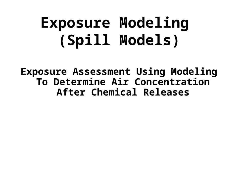
Constant Decay Model

FIGURE 3-3

0

10

20

30

40

50

60

0 10 20 30 40 50

Time in minutes

Co

nc

en

tra

tio

n in

mg

/m3

EXPOSURE MODELING

• Principles from physical chemistry are applied

• Applications will be presented in examples

• Graphical presentations from Dr. Mark Nicas – UC Berkeley are provided

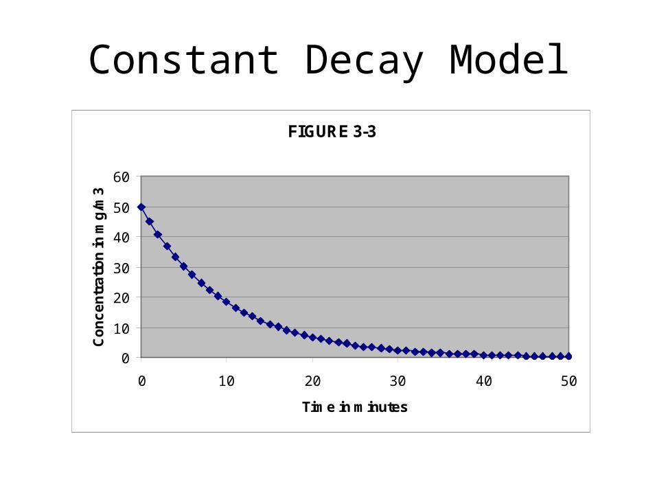
Elements of the Exposure Model

A chemical substance releaseA chemical substance release

Determine the air concentration from a release into a room

And

Estimate if the release may pose a probable risk inhalation health hazard.

Elements of the Exposure Model

An airborne exposure model uses the following elements:*

• The contaminant mass emission rate• The contaminant dispersion in a room• The employee exposure pattern *Source – OSHA TECHNICAL MANUAL ON

PHYSICAL – CHEMICAL MATHEMATICAL EXPOSURE MODELS

EXPOSURE ASSESSMENT

• When must an employer conduct an exposure assessment?– When there is a substance specific standard

(e.g. lead, methylene chloride)– When employees notice symptoms or complain

of respiratory effects– When the workplace contains visible emissions

(e.g. fumes, dust aerosols)

EXPOSURE ASSESSMENT

• OSHA Regulations for methods to determine employee exposure can be found for the following:– HAZWOPER – 29 CFR 1910.120– RESPIRATORS – 29 CFR 1910.134– SUBSTANCE SPECIFIC STANDARDS – 29

CFR 1910.1000 – 1052 (e.g. Formaldehyde)

EXPOSURE ASSESSMENT

• OSHA Regulations do not specify how the employer is to make a reasonable estimation for the purposes of selecting respirators for example (osha.gov/SLTC/respiratory_advisor)

• OSHA Substance Specific Standards allow for the use of ‘objective evidence’ to estimate exposure.

EXPOSURE ASSESSMENT

• When? What? How much employee exposure is there in the workplace?– Sampling – Personal exposure monitoring– Objective information – Data– Variation – Sampling + Data + Safety Factors

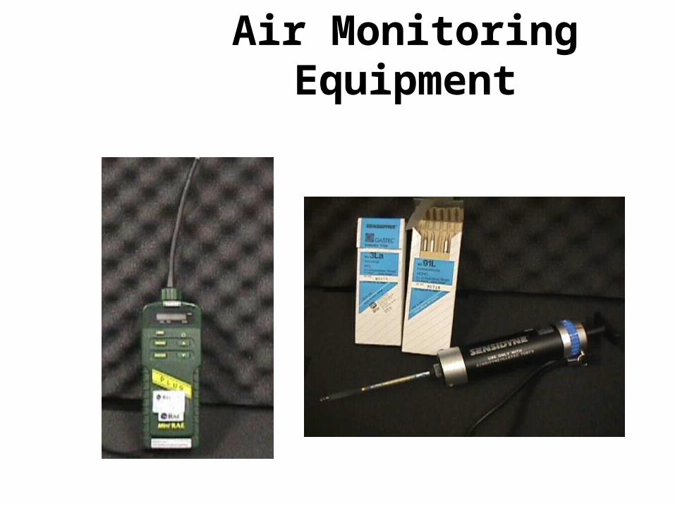
Air Monitoring Equipment

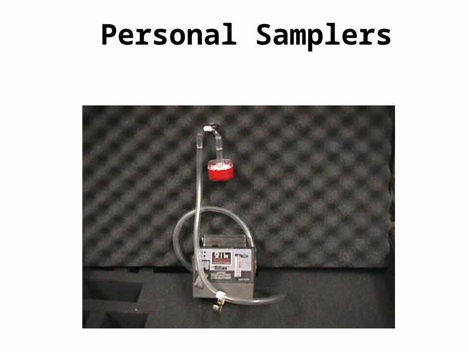
Personal Samplers

Personal Samplers- Media

Other TypesOther Typesofof

Site MonitoringSite Monitoring HAZCAT KitHAZCAT Kit Geiger CounterGeiger Counter - radiation- radiation Specialty MonitorsSpecialty Monitors - Passive monitoring badges- Passive monitoring badges - TIFF 5000- TIFF 5000

EXPOSURE ASSESSMENT

• BASIC TERMS– Exposure Model– Air Contaminants

• Parts Per Million

• Milligrams Per Cubic Meter

– Employee Exposure

EXPOSURE ASSESSMENT

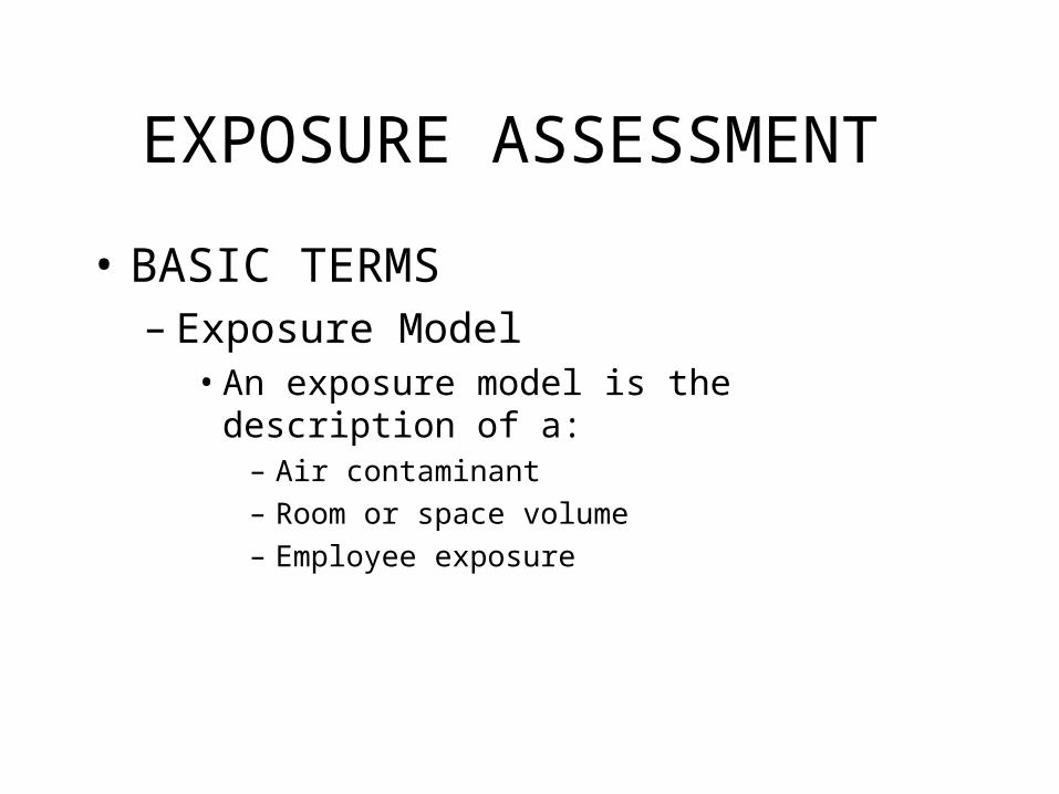
• BASIC TERMS– Exposure Model

• An exposure model is the description of a:– Air contaminant

– Room or space volume

– Employee exposure

EXPOSURE ASSESSMENT

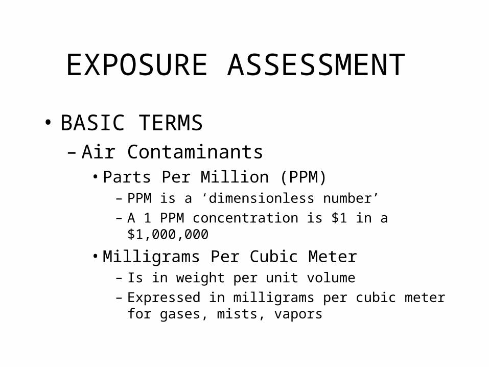
• BASIC TERMS– Air Contaminants

• Parts Per Million (PPM)– PPM is a ‘dimensionless number’

– A 1 PPM concentration is $1 in a $1,000,000

• Milligrams Per Cubic Meter– Is in weight per unit volume

– Expressed in milligrams per cubic meter for gases, mists, vapors

EXPOSURE ASSESSMENT

• BASIC TERMS– Employee Exposure

• Who, What, When, Why, How Exposed?

• ‘Typical’ or ‘Emergency’ release

• What is an ‘Incidental’ release as defined in the HAZWOPER regulation?

Chemical Identity and Form

        If the chemical is a gas – The molecular weight and the gas density

        If the chemical is a liquid – The molecular weight and the vapor pressure

        If the chemical is a solid – The molecular weight

Material Release Parameters

        The room or space volume (V) in cubic meters (m3)

        The room supply/exhaust air rate (Q) in cubic meters per minute (m3/min)

        The contaminant emission rate function (G) in milligrams per minute (mg/min)

Room Ventilation and Volume

V = Room volume determined by (Length X Width X Height)

Q = Air supply. It is assumed to be the room’s entire supply/exhaust air exchange rate from a mechanically – driven system. note: If room air supply is not known use the following assumptions**

**Air speed (s) = 3-4.5 m/min in a room with no strong air motion

Air speed (s) = 7.6 m/min in a room with strong air currents

Mass Emission Q = The product of the air speed times the room

area (Speed X Length X Width)

Gt = The emission rate function (Gt) is expressed in a release rate of mass-per-time or milligrams per minute (mg/min).

Air Concentration in a room after a release (C0) is a ‘worst case’ scenario of the Emission Rate Function over the Room Exhaust Rate or (Gt/Q)

‘Worst Case Scenerio’

• The air concentration (C0) of a release of a

material in a room using the Exposure Model Gt/Q is a ‘worst case’ scenario model

• Use the ideal gas law equation – (PV/nRT) to determine the concentration C0

‘Worst Case Scenerio’

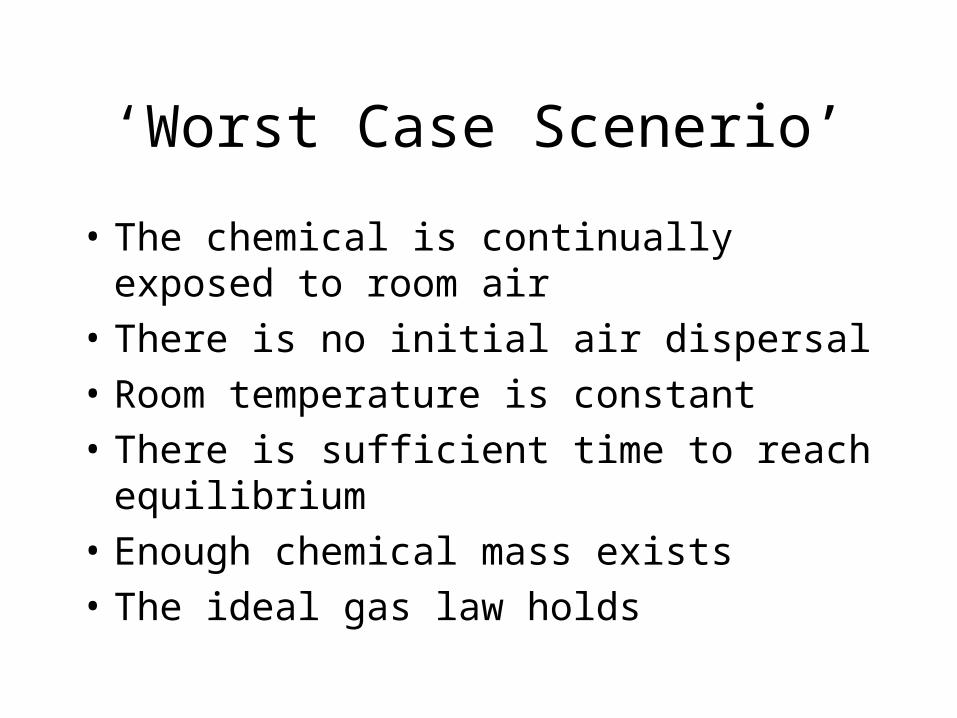
• The chemical is continually exposed to room air

• There is no initial air dispersal

• Room temperature is constant

• There is sufficient time to reach equilibrium

• Enough chemical mass exists

• The ideal gas law holds

Ideal Gas Law Background

• A variation of Boyle’s and Dalton’s lawsP1 V1 = P2 V2

T1 T2

PTOTAL = P1 + P2 + … + Pk, for k constituents

Application includes converting a mass of liquid evaporating per minute to the vapor volume evaporating per minute

Dalton’s Law

• The total pressure of a gaseous mixture is the sum of the partial pressures exerted by each constituent of the mixture– PTOTAL = P1 + P2 + … + Pk, for k constituents

• According to the ideal gas law, the mole fraction (Yi) of a gas constituent is

– Yi = Pi / PTOTAL , expressed in ppm (parts per million)

Ideal Gas Law Constants

• P = Pressure in mm Hg

• V = Volume in M3

• T = Temperature in K

• R = Gas Constant 0.623 mm Hg M3MOL-1K-1

• n = number of moles of gas

Ideal Gas Law

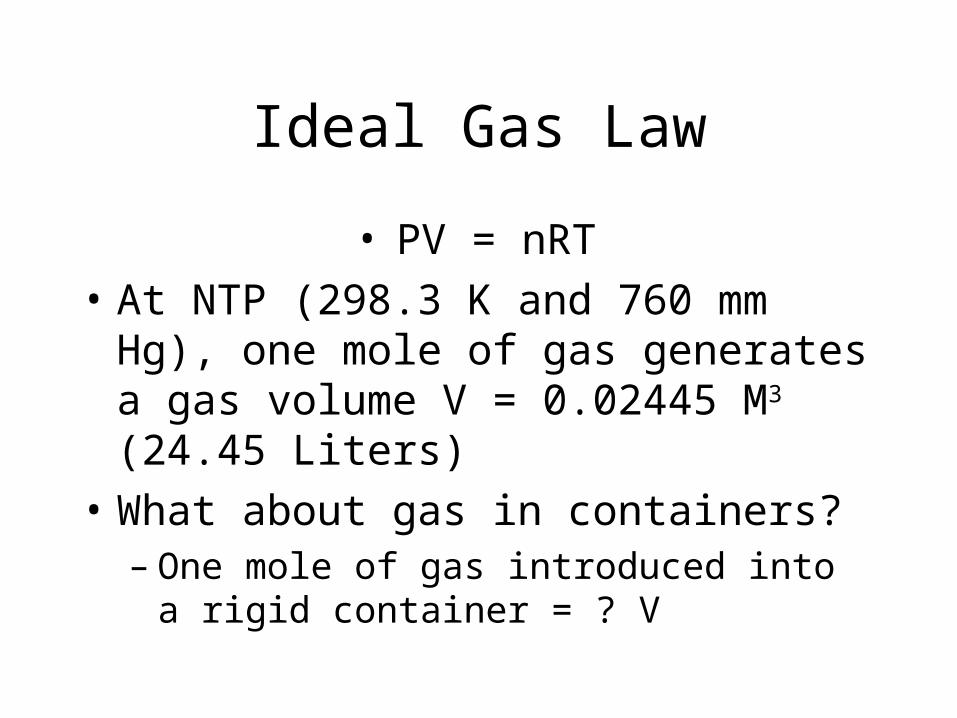
• PV = nRT

• At NTP (298.3 K and 760 mm Hg), one mole of gas generates a gas volume V = 0.02445 M3 (24.45 Liters)

• What about gas in containers?– One mole of gas introduced into a rigid

container = ? V

Ideal Gas Law

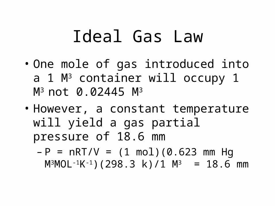
• One mole of gas introduced into a 1 M3 container will occupy 1 M3 not 0.02445 M3

• However, a constant temperature will yield a gas partial pressure of 18.6 mm – P = nRT/V = (1 mol)(0.623 mm Hg M3MOL-

1K-1)(298.3 k)/1 M3 = 18.6 mm

Vapor Volume

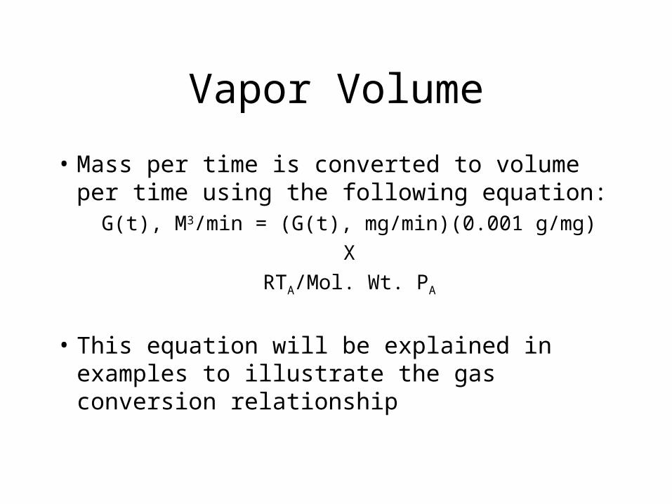
• Mass per time is converted to volume per time using the following equation:

G(t), M3/min = (G(t), mg/min)(0.001 g/mg)

X

RTA/Mol. Wt. PA

• This equation will be explained in examples to illustrate the gas conversion relationship

Vapor Pressure (Eq)

• When the rate of evaporation = rate of condensation in the headspace of containers– If the system is at equilibrium and the

headspace air is saturated with chemical vapor

• The partial pressure (Pv) of a chemical is related to the temperature, e.g. – Pv of benzene at 20 C is 75 mm Hg and 96 mm

Hg at 25 C

Saturation Concentration (Csat)

Csat in ppm

= PV in mm Hg X 106

760 mm Hg

• This unifies Boyle’s and Dalton’s Law into the ideal gas law

Saturation Concentration (Csat)

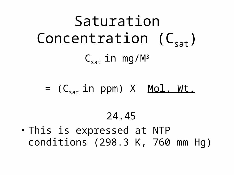
Csat in mg/M3

= (Csat in ppm) X Mol. Wt.

24.45

• This is expressed at NTP conditions (298.3 K, 760 mm Hg)

Saturation Concentration (Csat)

Csat in mg/M3

Can also be determined by the following:

= PV X Mol. Wt. X 1000RT

This is the product of the vapor pressure of n moles of gas and the chemical’s molecular

weight

Spill Modeling

• Example 1 – Estimate the air concentration using a ‘worse case scenario using an identified chemical and mass emission rate

• Example 2 – Determine the air concentration of a spill after one minute knowing the room volume and dispersal rate

Example #1 (C2Cl4 Release)

• A container of perchloroethylene (C2Cl4) is left open in a unventilated cabinet.

• An individual opens the door and is exposed

• What is the perchloroethylene concentration in ppm that the employee is exposed to?

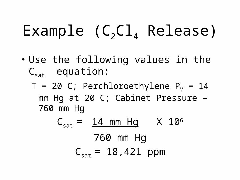
Example (C2Cl4 Release)

• Use the following values in the Csat equation:T = 20 C; Perchloroethylene PV = 14 mm Hg at

20 C; Cabinet Pressure = 760 mm Hg

Csat = 14 mm Hg X 106

760 mm Hg

Csat = 18,421 ppm

Dalton’s Law (Remember!!!)

• To be rigorous, one must add the partial pressure of the perchloroethylene to the total pressure in the cabinet.– This yields a Csat of 18,090 ppm (A 2%

difference)

• This estimate is based on a Qintial of 0, any air movement (Q) > 0 would revise the estimate of concentration downward.

Exposure Limits for C2Cl4

• For perchloroethylene (C2Cl4 ) the acceptable OSHA maximum peak is 300 ppm* * 29 CFR 1910.1000, Table Z-2

• The initial exposure concentration of 18,090 ppm C2Cl4 is 60 times greater than the acceptable ceiling limit.

Example #2 (Gas Release)

• Carbon Dioxide (CO2) is released into a

10 X 20 square meter (33 X 65 foot2) room from a 10 - liter container. How many parts per million (ppm) of CO2 are

released?

• Assume that the air speed in the room is 3 meters/minute.

Solution

• First, determine the molecular weight of Carbon Dioxide (CO2) in a molar unit (mole) of gas. It is the product of the gas molecules of carbon (C) and oxygen (O):

• C + O + O2 = 12 + 16 +16 or

44 milligrams CO2

Solution

• Then, assume that carbon dioxide gas occupies all of the container and all of the gas is released at once. The total volume of the container is 10 liters (L). The amount of gas released in cubic meters is as follows:

10 liters X cubic meter (M3)/ 1000 liters or 0.01 m3

Solution

• In a ‘normal’ temperature (T) and pressure (P) environment, a mole of gas occupies a volume (V) 0f 0.02445 M3 (24.45 L)

 The number (n) of moles of CO2 released is:

0.01 M3 CO2 / 0.02445 M3/mole

= 0.4 moles CO2

Answer

• To determine a ‘worst-case’ scenario, we first determine the partial pressure of the gas release in the room air.

Answer

• The partial pressure of the CO2 released

is determined using the ideal gas equation:

P = nRT/V

Temperature & Pressure

• Room temperatures must be converted to degrees Kelvin (K) using the ideal gas law, so room temperature in C is added to 273.3

• Pressure is expressed in milliliters of mercury (mm Hg)

Answer

• PCO2 = nRT/V

• P = (0.4 mole CO2)(0.0623 mm Hg . m3 .

mole-1 . K-1)(298.3 K)/ 0.01 M3

PCO2 = 0.025 / 0.01 mm Hg = 2.55 mm Hg

Answer

• P1 nRT/V/ P2 nRT/V

Partial Pressure = P1/ P2

Concentration is then expressed as the vapor volume of a chemical in its ratio to the vapor volume of air at atmospheric pressure (V/V).

Answer

The V/V application model is a ‘best-guess’ assumption of exposure. This is the estimated vapor volume of a contaminant in a million parts of air (ppm).

V/V – V/V – vapor pressure of contaminant vapor pressure of contaminant X 10X 1066

vapor pressure of airvapor pressure of air

Concentration (C0)

• The ‘worst-case concentration (C0) of

carbon dioxide released into the room is determined by the following equation:

(C0) = Partial Pressure/ Total Atmospheric

Pressure in a million parts of air (ppm)

Concentration (C0)

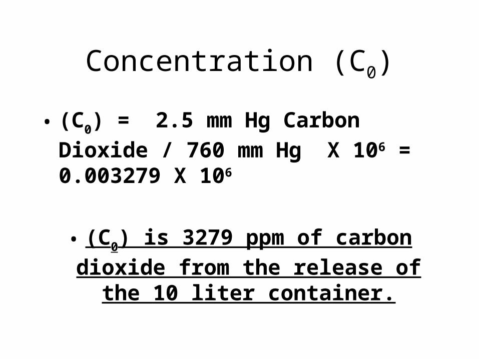
• (C0) = 2.5 mm Hg Carbon Dioxide / 760

mm Hg X 106 = 0.003279 X 106

• (C0) is 3279 ppm of carbon dioxide from

the release of the 10 liter container.

Concentration (Ct)

• (Ct) is the concentration at a time from the initial release C0 to a time t

• This takes into account diffusion of the release into a space by airflow 

Concentration (Ct)

• What is the expected air concentration of CO2

in the room after one minute or (Gt/Q)?

• Assume that in one minute the entire container is released or that 3279 ppm exists from the release. We need to determine the concentration of CO2 throughout the room.

Concentration (Ct)

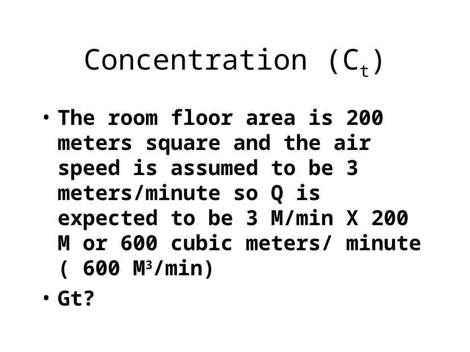
• The room floor area is 200 meters square and the air speed is assumed to be 3 meters/minute so Q is expected to be 3 M/min X 200 M or 600 cubic meters/ minute ( 600 M3/min)

• Gt?

Concentration (Ct)

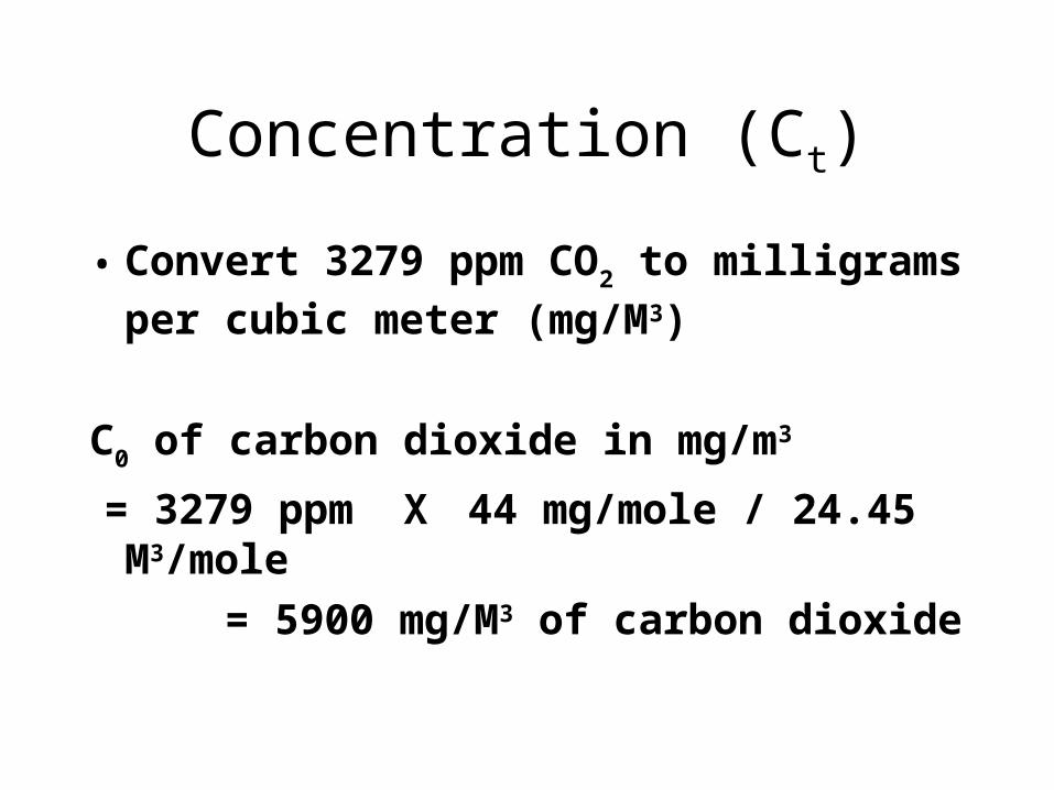
• Convert 3279 ppm CO2 to milligrams per

cubic meter (mg/M3)

C0 of carbon dioxide in mg/m3

= 3279 ppm X 44 mg/mole / 24.45 M3/mole

= 5900 mg/M3 of carbon dioxide

Concentration (Ct)

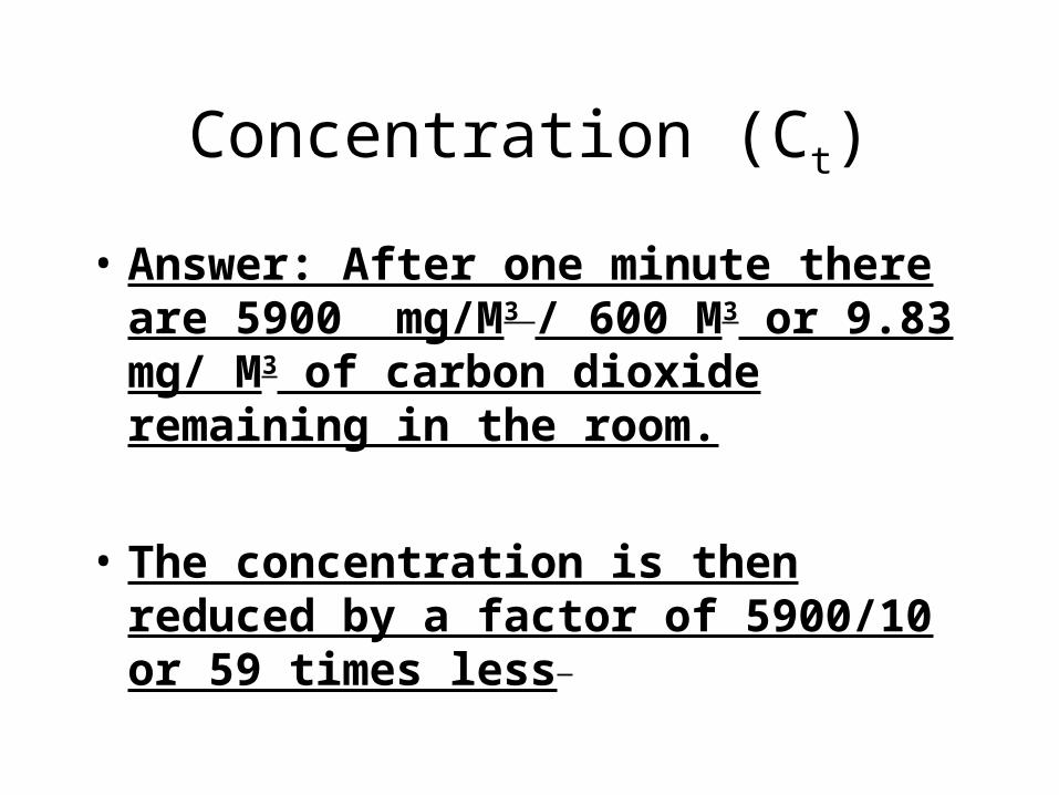
• Answer: After one minute there are 5900 mg/M3 / 600 M3 or 9.83 mg/ M3 of carbon dioxide remaining in the room.

• The concentration is then reduced by a factor of 5900/10 or 59 times less

Constant Decay Theory by Dr. Mark Nicas

• Applications:– Objective Exposure Assessment– Spill models from container filling– Confined Spaces?

• Exponential decay model with an initial concentration (Co)

Constant Decay Theory by Dr. Mark Nicas

÷÷ø

öççè

æ ×+-+

úúû

ù

êêë

é

÷÷ø

öççè

æ ×+--

×+

×+= t

V

Vk Q exp C t

V

Vk Q exp 1

Vk Q

QC G C(t) LL

L

IN0

CIN -- mg/m3 V -- m3

G -- mg/min kL -- per min

Q -- m3/min C0 -- mg/m3

Constant Decay

FIGURE 3-3

0

10

20

30

40

50

60

0 10 20 30 40 50

Time in minutes

Co

nc

en

tra

tio

n in

mg

/m3

Backpressure Effect on Contaminant Emission

• Applications:– Low vapor pressure chemicals < 1 mm Hg

• Pesticides

• Nerve Agents

• Net rate model with a steady state factor for chemicals with a low vapor pressure at equilibrium

Backpressure Effect on Contaminant Emission

Ct -- mg/m3 V -- m3

G0 -- mg/min t -- min

Q -- m3/min Csat -- mg/m3

úû

ùêë

é÷÷ø

öççè

æ×

××

--×= tCV

CQ +Gexp 1

C

G + Q

G C(t)

sat

sat0

sat

0

0

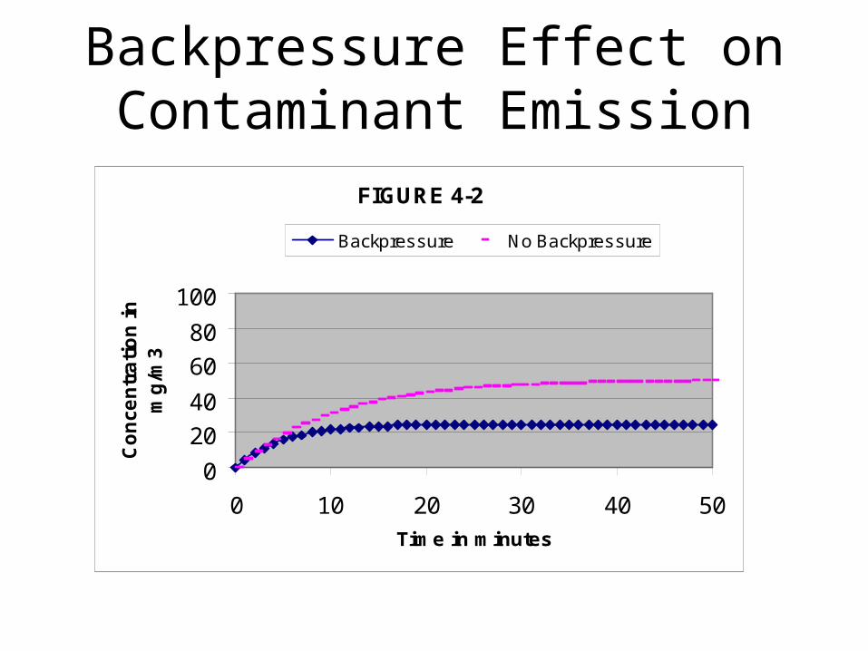
Backpressure Effect on Contaminant Emission

FIGURE 4-2

0

20

40

60

80

100

0 10 20 30 40 50

Time in minutes

Co

nce

ntr

ati

on

in

m

g/m

3

Backpressure No Backpressure

NEAR / FAR FIELD (NF/ FF) with constant contaminant

emission rate• Applications:

– Operations with Dilution Ventilation– Assume a well mixed room dispersion pattern

• Model describes zonal concentration in the near hemispherical free surface area and an air flow rate to a far field

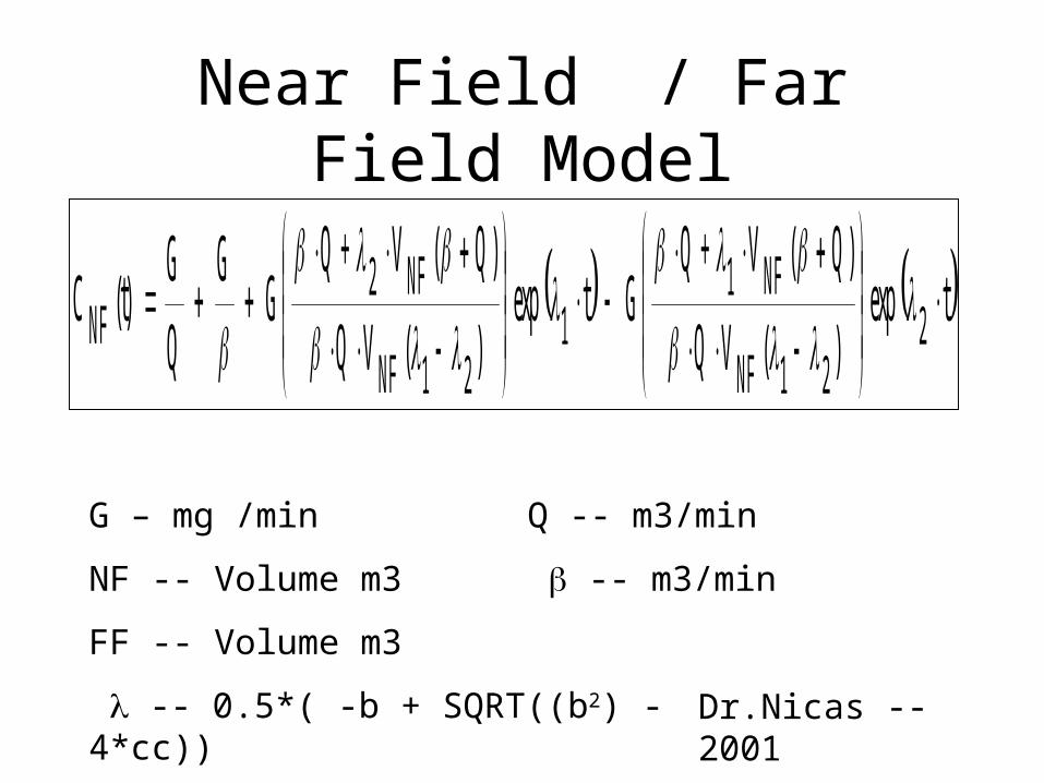
Near Field / Far Field Model

Dr.Nicas -- 2001

G – mg /min Q -- m3/min

NF -- Volume m3 -- m3/min

FF -- Volume m3

-- 0.5*( -b + SQRT((b2) - 4*cc))

texp )(VQ

)Q(V + QG texp

)(VQ

)Q(V + QG

G

Q

G (t)C 2

21NF

NF11

21NF

NF2NF ×÷

÷ø

öççè

æ

-××

+××-×÷

÷ø

öççè

æ

-××

+××++=

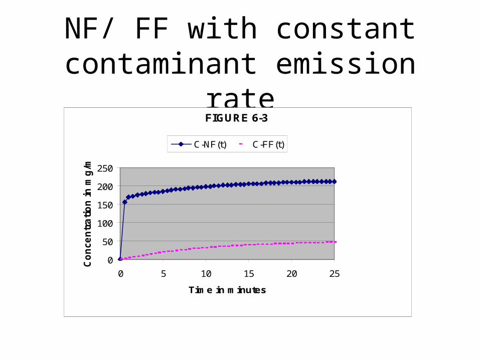
NF/ FF with constant contaminant emission rate

FIGURE 6-3

0

50

100

150

200

250

0 5 10 15 20 25

Time in minutes

Co

nce

ntr

ati

on

in

mg

/m3

C-NF(t) C-FF(t)

Spherical Turbulent Diffusion – Pulse Release

• Applications: – Operations with Local Exhaust Ventilation– Storage tank filling operations in buildings

• Models apply turbulent eddy diffusion for a continuous concentration near an emission source

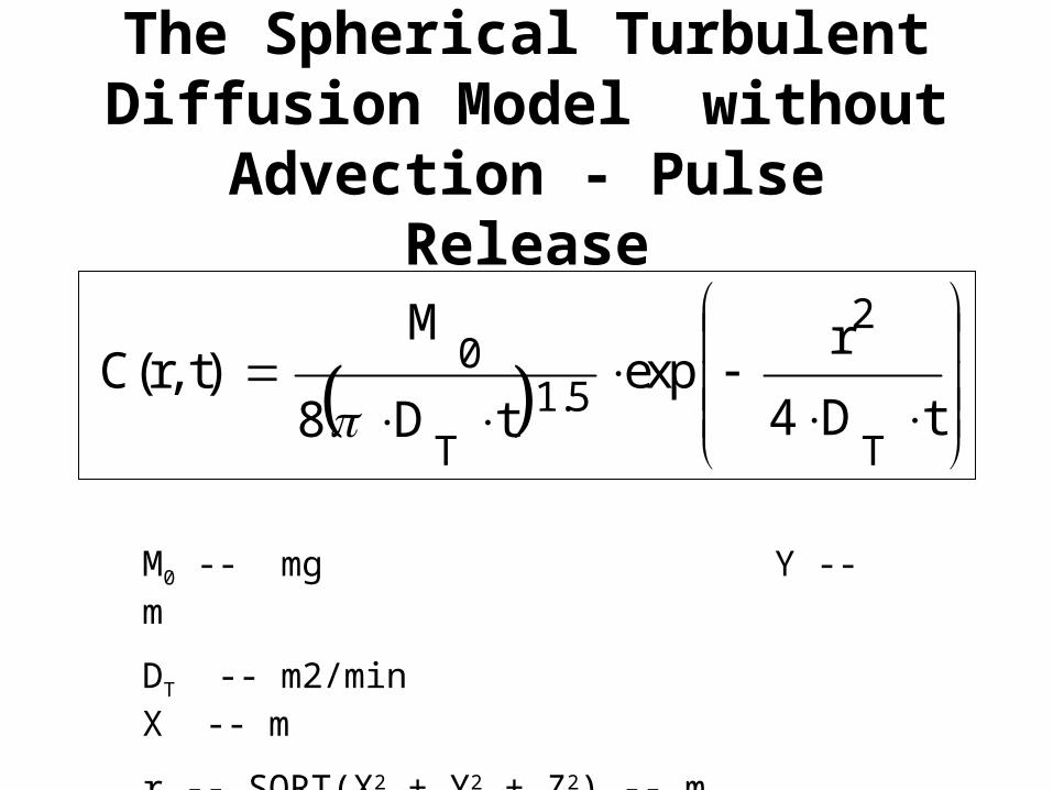
The Spherical Turbulent Diffusion Model without Advection - Pulse

Release

÷÷÷

ø

ö

ççç

è

æ

××-×

××=

tD4

r exp tD8

M t)C(r,

T

2

5.1T

0

p

M0 -- mg Y -- m

DT -- m2/min X -- m

r -- SQRT(X2 + Y2 + Z2) -- m Z -- m

Spherical Turbulent Diffusion – Pulse Release

FIGURE 8-2

0

50

100

150

200

250

300

0 1 2 3 4 5

Time in minutes

Co

nc

en

tra

tio

n in

mg

/m3