Politically feasible reforms of non-linear tax systems * Felix J. Bierbrauer † Pierre C. Boyer ‡ July 11, 2017 Abstract We present a conceptual framework for the analysis of politically feasible tax reforms. First, we prove a median voter theorem for monotonic reforms of non- linear tax systems. This yields a characterization of reforms that are preferred by a majority of individuals over the status quo and hence politically feasible. Second, we show that every Pareto-efficient tax systems is such that moving towards lower tax rates for below-median incomes and towards higher rates for above median incomes is politically feasible. Third, we develop a method for diagnosing whether a given tax system admits reforms that are welfare-improving and/ or politically feasible. Keywords: Non-linear income taxation; Tax reforms; Political economy, Welfare analysis. JEL classification: C72; D72; D82; H21. * We thank Laurent Bouton, Micael Castanheira, Vidar Christiansen, Antoine Ferey, Sidartha Gor- don, Bard Harstad, Emanuel Hansen, Bas Jacobs, Laurence Jacquet, Yukio Koriyama, ´ Etienne Lehmann, Jean-Baptiste Michau, Benny Moldovanu, Massimo Morelli, Andreas Peichl, Carlo Prato, Anasuya Raj, Alessandro Riboni, Dominik Sachs, Johannes Spinnewijn, Stefanie Stantcheva, Aleh Tsyvinski, Paul- Armand Veillon, Marius Vogel, John Weymark, Nicolas Werquin, Jan Zapal, and Floris Zoutman. We also appreciate the comments of seminar and conference audiences at Yale, Paris-Dauphine, Oslo, Cologne, CREST- ´ Ecole Polytechnique, Leuven, Paris Fiscal Study Group, CESifo Area Conference on Public Sector Economics, and PET 2017. The authors gratefully acknowledge the Max Planck Institute in Bonn for hospitality and financial support, and the Investissements d’Avenir (ANR-11-IDEX-0003/Labex Ecodec/ANR-11-LABX-0047) for financial support. † CMR - Center for Macroeconomic Research, University of Cologne, Albert-Magnus Platz, 50923 K¨ oln, Germany. E-mail: [email protected] ‡ CREST, ´ Ecole Polytechnique, Universit´ e Paris-Saclay, Route de Saclay, 91128 Palaiseau, France. E-mail: [email protected]

Welcome message from author
This document is posted to help you gain knowledge. Please leave a comment to let me know what you think about it! Share it to your friends and learn new things together.
Transcript

Politically feasible reforms of non-linear tax systems∗
Felix J. Bierbrauer† Pierre C. Boyer‡
July 11, 2017
Abstract
We present a conceptual framework for the analysis of politically feasible tax
reforms. First, we prove a median voter theorem for monotonic reforms of non-
linear tax systems. This yields a characterization of reforms that are preferred by
a majority of individuals over the status quo and hence politically feasible. Second,
we show that every Pareto-efficient tax systems is such that moving towards lower
tax rates for below-median incomes and towards higher rates for above median
incomes is politically feasible. Third, we develop a method for diagnosing whether
a given tax system admits reforms that are welfare-improving and/ or politically
feasible.
Keywords: Non-linear income taxation; Tax reforms; Political economy, Welfare
analysis.
JEL classification: C72; D72; D82; H21.
∗We thank Laurent Bouton, Micael Castanheira, Vidar Christiansen, Antoine Ferey, Sidartha Gor-
don, Bard Harstad, Emanuel Hansen, Bas Jacobs, Laurence Jacquet, Yukio Koriyama, Etienne Lehmann,
Jean-Baptiste Michau, Benny Moldovanu, Massimo Morelli, Andreas Peichl, Carlo Prato, Anasuya Raj,
Alessandro Riboni, Dominik Sachs, Johannes Spinnewijn, Stefanie Stantcheva, Aleh Tsyvinski, Paul-
Armand Veillon, Marius Vogel, John Weymark, Nicolas Werquin, Jan Zapal, and Floris Zoutman.
We also appreciate the comments of seminar and conference audiences at Yale, Paris-Dauphine, Oslo,
Cologne, CREST-Ecole Polytechnique, Leuven, Paris Fiscal Study Group, CESifo Area Conference on
Public Sector Economics, and PET 2017. The authors gratefully acknowledge the Max Planck Institute in
Bonn for hospitality and financial support, and the Investissements d’Avenir (ANR-11-IDEX-0003/Labex
Ecodec/ANR-11-LABX-0047) for financial support.†CMR - Center for Macroeconomic Research, University of Cologne, Albert-Magnus Platz, 50923
Koln, Germany. E-mail: [email protected]‡CREST, Ecole Polytechnique, Universite Paris-Saclay, Route de Saclay, 91128 Palaiseau, France.
E-mail: [email protected]

1 Introduction
We study reforms of non-linear income tax systems from a political economy perspective.
Starting from a given status quo we characterize reforms that are politically feasible in the
sense that a majority of taxpayers will be made better off. In addition, we relate the set of
politically feasible reforms to the set of welfare-improving reforms. We thereby introduce
a conceptual framework that can be used to analyze whether welfare-improving reforms
have a chance in the political process. This framework can also be used to check whether
a given tax system is efficient in the sense that the scope for politically feasible welfare
improvement has been exhausted, or whether there is room for welfare-improvements
that will be supported by a majority of taxpayers.
The analysis of politically feasible reforms is made tractable by focussing on monotonic
reforms, i.e. on reforms such that the change in tax payments is a monotonic function
of income. We prove a median voter theorem according to which a monotonic reform is
politically feasible if and only if it is supported by the taxpayer with median income. The
key insight that enables a proof of the theorem is that the Spence-Mirrlees single crossing
property translates into a single-crossing property of preferences over monotonic reforms.
Thus, if the median voter benefits from a monotonic reform, then all taxpayers with a
higher or all tax payers with a lower income will also benefit, implying majority-support
for the reform.
Monotonic reforms play a prominent role in the theory of welfare-maximizing taxation.
Characterizations of optimal tax systems via the perturbation method often look at the
welfare implications of reforms that are monotonic (typically raising the marginal tax
rate in a small band of incomes). A welfare-maximizing tax system then has the property
that no such reform yields a welfare improvement. By relating our analysis of politically
feasible reforms to this approach we can look at the intersection of politically feasible
and welfare-improving reforms. We also argue that observed tax reforms are typically
monotonic reforms and provide examples from the US, Germany and France.
A simple graphical analysis enables us to diagnose whether a given status quo tax
system can be reformed in a politically feasible or welfare-improving way. We derive
sufficient statistics that admit a characterization in terms of auxiliary tax schedules. To
see whether, say, an increase of marginal tax rates for incomes in a certain range would be
politically feasible we can simply look at a graph that plots the status quo and an auxiliary
tax schedule for politically feasible reforms. If, for the given range of incomes, tax rates in
the status quo are below those stipulated by the auxiliary schedule, then moving towards
higher marginal tax rates is politically feasible. If they lie above, moving towards lower
rates will be politically feasible. We can use this approach also to diagnose whether there
is scope for revenue-increasing, Pareto-improving or welfare-improving reforms.
The characterization of politically feasible reforms shows that there are two Pareto
bounds for marginal tax rates. If marginal tax rates in the status quo exceed the upper
1

bound then lowering tax rates is Pareto-improving and hence politically feasible. Sim-
ilarly, if marginal tax rates fall short of the lower bound then an increase of tax rates
is Pareto-improving and hence politically feasible. If the status quo is Pareto-efficient
in the sense that marginal tax rates lie between those bounds, then a reform that raises
marginal tax rates for above median incomes and reforms that lower marginal tax rates
for below median incomes are politically feasible.
The marked discontinuity at the median level of income provides a possible explana-
tion for the observation that actual tax schedules often have a pronounced increase of
marginal tax rates close to the median income: if political economy forces push towards
low tax rates below the median and towards high tax rates above the median, then there
has to be an intermediate range that connects the low rates below the median with the
high rates above the median.
Our derivation of sufficient statistics for politically feasible or welfare-improving re-
forms is based on an analysis of reforms that involve a change of marginal tax rates that
applies only to incomes in a certain bracket. More specifically, it is based on an analysis
of small reforms. They are small in that we look at the implications of a marginal change
of tax rates applied to a bracket of incomes with vanishing length. However, our analysis
is explicit about the transition from a large reform that involves a discrete change of
marginal tax rates applied to a non-negligible range of incomes to a reform that involves
only a marginal change of tax rates, but applied to a non-negligible range of incomes,
and, finally, to a reform that involves a marginal change of tax rates for a negligible range
of incomes. We believe that this derivation is of pedagogical value. It complements both
the heuristic approaches due to Piketty (1997) and Saez (2001) and approaches that make
use of functional derivatives such as Golosov, Tsyvinski and Werquin (2014) and Jacquet
and Lehmann (2016).
The remainder is organized as follows. The next section discusses related literature.
The formal framework is introduced in Section 3. Our analysis is based on a generic
Mirrleesian model of income taxation. Section 4 presents median voter theorems for
monotonic reforms. The characterization of politically feasible and welfare improving
reforms by means of sufficient statistics can be found in Section 5. Section 6 shows
that the median voter theorem for monotonic reforms extends to models of taxation
that are richer than the basic setup due to Mirrlees (1971). Specifically, we consider
the possibility to mix direct and indirect taxes as in Atkinson and Stiglitz (1976), the
possibility to add sources of heterogeneity among individuals such as fixed costs of labor
market participation or public goods preferences, and the possibility that taxpayers seek
to mitigate income differences that are due to luck as opposed to effort, as in Alesina and
Angeletos (2005). The last section contains concluding remarks. Unless stated otherwise,
proofs are relegated to the Appendix.
2

2 Related literature
The Mirrleesian framework is the workhorse for the normative analysis of non-linear tax
systems, see Hellwig (2007) and Scheuer and Werning (2016) for more recent analyses of
this model and Piketty and Saez (2013) for a literature review.
Saez and Stantcheva (2016) study generalized welfare functions with weights that
need not be consistent with the maximization of a utilitarian social welfare function. The
generalized weights may as well reflect alternative, non-utilitarian value judgments or po-
litical economy forces. Saez and Stantcheva emphasize the similarities between utilitarian
welfare maximization and political economy considerations: both can be represented as
resulting from the maximization of a generalized welfare function. Our approach takes
an alternative route and emphasizes the differences between the requirements of politi-
cally feasibility and welfare maximization. We distinguish the set of politically feasible
reforms from the set of welfare-improving reforms so as to be able to provide possibility
and impossibility results for politically feasible welfare-improvements.
Well-known political economy approaches to redistributive income taxation have used
the model of linear income taxation due to Sheshinski (1972). In this model, marginal
tax rates are the same for all levels of income and the resulting tax revenue is paid out as
uniform lump-sum transfers. As has been shown by Roberts (1977), the median voter’s
preferred system is a Condorcet winner in the set of all linear income tax systems (see,
e.g., Drazen, 2000; Persson and Tabellini, 2000). Our finding that a median voter theorem
applies to monotonic reforms of non-linear tax systems generalizes results by Rothstein
(1990; 1991) and Gans and Smart (1996) who focussed on linear tax systems.
Median voter theorems for linear income taxation have been widely used on the as-
sumption that voters are selfish. A prominent example is the prediction due to Meltzer
and Richard (1981) that tax rates are an increasing function of the difference between
median and average income. The explanatory power of this framework was found to be
limited – see, for instance, the review in Acemoglu, Naidu, Restrepo and Robinson (2015)
– and has led to analyses in which the preferences for redistributive tax policies are also
shaped by prospects for upward mobility or a desire for a fair distribution of incomes.1
In Section 6 we extend our basic analysis and prove a median voter theorem for reforms
of non-linear tax systems that takes account of such demands for fairness.
We derive sufficient statistics that enable us to identify reforms that are in the median
voter’s interest and would therefore be supported by a majority of voters. The relevant
sufficient statistics takes the form of an auxiliary tax schedule. The auxiliary schedule in
turn has properties which are similar to the work of Roell (2012) and Brett and Weymark
(2017; 2016) who characterize the non-linear income tax schedule that the median voter
would pick if she could dictate tax policy. Both schedules reveal that the median voter
1See, for instance, Piketty (1995), Benabou and Ok (2001), Alesina and Angeletos (2005), Benabou
and Tirole (2006), or Alesina, Stantcheva and Teso (2017).
3

wants to have low taxes on the poor and high taxes on the rich. For the special case
of quasi-linear utility functions, the auxiliary schedule indeed coincides with the median
voter’s preferred schedule whenever the latter does not give rise to bunching.
A classical idea in public finance is that the theory of optimal taxation – which
characterizes welfare-maximizing tax systems and has no role for current tax policy –
should be complemented by a theory of tax reforms with a focus on incremental changes
that apply to a given status quo, see Feldstein (1976). Weymark (1981) studies the scope
for Pareto-improving reforms of a commodity tax system. To give another example,
Guesnerie (1995) contains an analysis of tax reforms that emphasizes political economy
forces, formalized as a requirement of coalition-proofness, that affect the implementability
of reforms. Our analysis contributes to this earlier literature by combining results from
social choice theory on the applicability of median voter theorems with the perturbation
approach to the analysis of non-linear tax systems. Our main results in Theorems 1
and 2 provide a characterization of politically feasible reforms of non-linear tax systems.
Getting there requires arguments from both strands of the literature.
The focus on the conditions under which a status quo tax policy admits reforms that
are politically feasible distinguishes our work from papers that explicitly analyze political
competition as a strategic game and then characterize equilibrium tax policies.2
Our analysis of welfare-improving reforms can be related to a literature that seeks to
identify society’s social welfare function empirically.3 Through the lens of our model, this
literature can alternatively be interpreted as identifying the set of social welfare functions
for which a given reform – e.g. an increase of marginal tax rates for incomes close to the
sixtieth-percentile of the income distribution – would be welfare-improving.
3 The model
3.1 Preferences
There is a continuum of individuals of measure 1. Individuals are confronted with a
predetermined income tax schedule T0 that assigns a (possibly negative) tax payment
2Examples include Acemoglu, Golosov and Tsyvinski (2008; 2010) who relate dynamic problems of
optimal taxation to problems of political agency as in Barro (1973) and Ferejohn (1986); Farhi, Sleet,
Werning and Yeltekin (2012) and Scheuer and Wolitzky (2016) who study optimal capital taxation sub-
ject to the constraints from probabilistic voting as in Lindbeck and Weibull (1987); Battaglini and Coate
(2008) who study optimal taxation and debt financing in a federal system using the model of legisla-
tive bargaining due to Baron and Ferejohn (1989); Bierbrauer and Boyer (2016) who study Downsian
competition with a policy space that includes non-linear tax schedules and possibilities for pork-barrel
spending as in Myerson (1993). Ilzetzki (2015) studies reforms of the commodity tax system using a
model of special interests politics.3See, for instance, Christiansen and Jansen (1978), Blundell, Brewer, Haan and Shephard (2009),
Bourguignon and Spadaro (2012), Bargain, Dolls, Neumann, Peichl and Siegloch (2011), Hendren (2014),
Zoutman, Jacobs and Jongen (2014), Lockwood and Weinzierl (2016), or Bastani and Lundberg (2016).
4

T0(y) to every level of pre-tax income y ∈ R+. Under the initial tax system individuals
with no income receive a transfer equal to c0 ≥ 0. We assume that T0 is everywhere
differentiable so that marginal tax rates are well-defined for all levels of income. We also
assume that y − T0(y) is a non-decreasing function of y and that T0(0) = 0.
Individuals have a utility function u that is increasing in private goods consumption, or
after-tax income, c, and decreasing in earnings or pre-tax income y. Utility also depends
on a measure of the individual’s productive ability, referred to as the individual’s type.
The set of possible types is denoted by Ω and taken to be a compact subset of the non-
negative real numbers, Ω = [ω, ω] ⊂ R+. A typical element of Ω will be denoted by ω.
The utility that an individual with type ω derives from c and y is denoted by u(c, y, ω).
The cross-section distribution of types in the population is represented by a cumulative
distribution function F with density f . We write ωx for the skill type with F (ωx) = x.
For x = 12, this yields the median skill type also denoted by ωM .
The slope of an individual’s indifference curve in a y-c-diagram −uy(c,y,ω)
uc(c,y,ω)measures
how much extra consumption an individual requires as a compensation for a marginally
increased level of pre-tax income. We assume that this quantity is decreasing in the
individual’s type, i.e. for any pair (c, y) and any pair (ω, ω′) with ω′ > ω,
−uy(c, y, ω′)
uc(c, y, ω′)≤ −uy(c, y, ω)
uc(c, y, ω).
This assumption is commonly referred to as the Spence-Mirrlees single crossing property,
see Figure 5 (left panel).
Occasionally, we illustrate our results by looking at more specific utility functions. One
case of interest is the specification of a utility function U : R2+ → R so that u(c, y, ω) =
U(c, y
ω
). We can then interpret ω as an hourly wage and l = y
ωas the time that an
individual needs to generate a pre-tax-income of y. Another case of interest is the quasi-
linear in private goods consumption specification so that u(c, y, ω) = c − k(y, ω). The
function k then gives the cost of productive effort. If we combine both cases utility can
be written as c− k(yω
), where the function k is taken to be increasing and convex. The
cost function k is said to be iso-elastic if it takes the form k(yω
)=(yω
)1+ 1ε , for some
parameter ε > 0.
We assume that leisure is a non-inferior good. If individuals experience an increase in
an exogenous source of income e, they do not become more eager to work. More formally,
we assume that for any pair (c, y) any ω and any e′ > e,
−uy(c+ e, y, ω)
uc(c+ e, y, ω)≤ −uy(c+ e′, y, ω)
uc(c+ e′, y, ω).
We can also express this condition by requiring that, for any combination of c, y, e and ω,
the derivative of −uy(c+e,y,ω)
uc(c+e,y,ω)with respect to e is non-negative. This yields the following
condition: for all c, y, e and ω,
−ucc(c+ e, y, ω)uy(c+ e, y, ω)
uc(c+ e, y, ω)+ ucy(c+ e, y, ω) ≤ 0 . (1)
5

Finally, we assume that an individual’s marginal utility of consumption uc(c, y, ω) is
both non-increasing in c and non-increasing in ω, i.e. ucc(c, y, ω) ≤ 0 and ucω(c, y, ω) ≤0. These assumptions hold for any utility function u(c, y, w) = v(c) − k(y, ω) that is
additively separable between private goods consumption c on the one hand and the pair
(y, ω) on the other, where v is a (weakly) concave function. With u(c, y, ω) = U(c, y
ω
),
ucω(c, y, ω) ≤ 0 holds provided that Ucl(c, y
ω
)≥ 0 so that working harder makes you more
eager to consume.4
3.2 Reforms
A reform induces a new tax schedule T1 that is derived from T0 so that, for any level of
pre-tax income y, T1(y) = T0(y) + τ h(y), where τ is a scalar and h is a function. We
represent a reform by the pair (τ, h). Without loss of generality, we focus on reforms such
that y − T1(y) is non-decreasing. The reform induces a change in tax revenue denoted
by ∆R(τ, h). For now we assume that this additional tax revenue is used to increase the
basic consumption level c0. Alternatives are considered in Section 6.
y
c
C1(y)
C0(y)
c0 + ∆R
c0
c0 + ∆R − τ(yb − ya)
ya yb
Figure 1: A reform in the (τ, ya, yb)-class
Some of our results follow from looking at a special class of reforms. For this class,
there exists a first threshold level of income ya, so that the new and the old tax schedule
coincide for all income levels below the threshold, T0(y) = T1(y) for all y ≤ ya. There
exists a second threshold yb > ya so that for all incomes between ya and yb marginal tax
rates are increased by τ , T ′0(y) + τ = T ′1(y) for all y ∈ (ya, yb). For all incomes above yb,
marginal tax rates coincide, so that T ′0(y) = T ′1(y) for all y ≥ yb. Hence, the function h
4Seade (1982) refers to Ucl(c, yω
)≥ 0 as non-Edgeworth complementarity of leisure and consumption.
6

is such that
h(y) =
0, if y ≤ ya ,
y − ya, if ya < y < yb ,
yb − ya, if y ≥ yb .
For reforms of this type we will write (τ, ya, yb) rather than (τ, h). Figure 1 shows how
a reform in the (τ, ya, yb)-class affects the combinations of consumption c and earnings y
that are available to individuals. Specifically, the figure shows the curves
C0(y) = c0 + y − T0(y), and C1(y) = c0 + ∆R + y − T0(y)− τh(y) .
Part A of the Appendix contains a detailed analysis of the behaviorial responses to such
reforms that takes account of the bunching that results from the kink in the tax schedule
generated by the reform.
Reforms of the (τ, ya, yb)-type play a prominent role in the literature. Papers that use
functional derivatives to analyze tax perturbations rest, however, on the assumption that
both pre- and post-reform earnings are characterized by first order conditions. Reforms
in the (τ, ya, yb)-class can not be approached directly with this approach. Instead one
looks at smooth reforms that approximate such reforms. The formal analysis that follows
applies both to reforms in the (τ, ya, yb)-class and to reforms where pre- and post-reform
earnings follow from first order conditions. In the remainder and without further mention
we focus on these two classes of reforms.
Notation. To describe the implications of reforms for measures of revenue, welfare and
political support it proves useful to introduce the following optimization problem: choose
y so as to maximize
u (c0 + e+ y − T0(y)− τh(y), y, ω) , (2)
where e is a source of income that is exogenous from the individual’s perspective. We
assume that this optimization problem has, for each type ω, a unique solution that we
denote by y∗(e, τ, ω).5 The corresponding indirect utility level is denoted by V (e, τ, ω).
Armed with this notation we can express the reform-induced change in tax revenue as
∆R(τ, h) :=
∫ ω
ω
T1(y∗(∆R(τ, h), τ, ω))− T0(y∗(0, 0, ω))f(ω) dω .
The reform-induced change in indirect utility for a type ω individual is given by
∆V (ω | τ, h) := V (∆R(τ, h), τ, ω)− V (0, 0, ω) .
5For ease of exposition, we ignore the non-negativity constraint on y in the body of the text and
relegate this extension to part C in the Appendix. There, we clarify how the analysis has to be modified
if there is a set of unemployed individuals whose labor market participation might be affected by a
reform.
7

Pareto-improving reforms. A reform (τ, h) is said to be Pareto-improving if, for all
ω ∈ Ω, ∆V (ω | τ, h) ≥ 0, and if this inequality is strict for some ω ∈ Ω.
Welfare-improving reforms. We consider a class of social welfare functions. Mem-
bers of this class differ with respect to the specification of welfare weights. Admissi-
ble welfare weights are represented by a non-increasing function g : Ω → R+ with the
property that the average welfare weight equals 1,∫ ωωg(ω)f(ω)dω = 1 . We denote by
G(ω) :=∫ ωωg(s) f(s)
1−F (ω)ds the average welfare weight among individuals with types above
ω. Note that, if g is strictly decreasing, then G(ω) < 1, for all ω > ω. For a given
function g, the welfare change that is induced by a reform is given by
∆W (g | τ, h) :=
∫ ω
ω
g(ω)∆V (ω | τ, h)f(ω) dω .
A reform (τ, h) is said to be welfare-improving if ∆W (g | τ, h) > 0.
Political support for reforms. Political support for the reform is measured by the
mass of individuals who are made better if the initial tax schedule T0 is replaced by T1,
S(τ, h) :=
∫ ω
ω
1∆V (ω | τ, h) > 0f(ω) dω ,
where 1· is the indicator function. A reform (τ, h) is said to be supported by a majority
of the population if S(τ, h) ≥ 12.
3.3 Types and earnings
Earnings depend inter alia on the individuals’ types in our framework. However, observed
tax policies express marginal tax rates as a function of income. To relate the results
from our theoretical analysis to observed tax policies we repeatedly invoke the function
y0 : Ω → R+ where y0(ω) = y∗(0, 0, ω) gives earnings as a function of type in the status
quo. We denote the inverse of this function by ω0 so that ω0(y) is the type who earns an
income of y in the status quo.
By the Spence-Mirrlees single crossing property the function y0 is weakly increasing.
The existence of its inverse ω0 requires in addition that, under the status quo schedule
T0, there is no bunching so that different types choose different levels of earnings.
Assumption 1 The function y0 is strictly increasing.
It is not difficult to relax this assumption. However, taking account of bunching in the
status quo requires additional steps in the formal analysis that we relegate to part C
of the Appendix. This extension is relevant because empirically observed tax schedules
frequently have kinks and hence give rise to bunching, see e.g. Saez (2010) and Kleven
(2016).
8
In principle, the functions y0 and ω0 could be estimated from any data set that
contains both data on individual earnings and productive abilities. In the original analysis
of Mirrlees (1971) hourly wages are taken to be the measure of productive abilities. Our
framework is consistent with this approach, but is also compatible with other measures
of ability.
When we illustrate our formal results by means of examples, we will assume that
both the distributions of earnings and the distribution of productive abilities are Pareto
distributions.6 Under these assumptions, earnings are an iso-elastic function of types, see
the following remark.
Remark 1 Suppose that the type distribution is a Pareto distribution that is represented
by the cdf F (ω) = 1−(ωminω
)a. Also suppose that, under the status quo tax schedule T0,
the earnings distribution is a Pareto-distribution with cdf F 0(y) = 1 −(yminy
)b, where
ymin > 0 and ωmin > 0. Then, for some multiplicative constant α,
y0(ω) = α ωγ and ω0(y) =( yα
) 1γ, where γ =
a
b.
4 Median voter theorems for monotonic reforms
4.1 Monotonic reforms
A tax reform (τ, h) is said to be monotonic over a range of incomes Y ⊂ R+ if
T1(y)− T0(y) = τ h(y)
is a monotonic function for y ∈ Y . Obviously, this is the case if h is monotonic for y ∈ Y .
We say that a reform is monotonic if h is monotonic over R+. Given a cross-section
distribution of income, we say that a reform is monotonic above (below) the median if
h(y) is a monotonic function for incomes above (below) the median income.
Monotonic reforms in research on tax systems. Monotonic reforms play a promi-
nent role in the literature. For instance, the characterization of a welfare-maximizing
tax systems in Saez (2001) is based on reforms in the (τ, ya, yb)-class. This is a class of
monotonic reforms. Political economy analysis in the tradition of Roberts (1977) and
Meltzer and Richard (1981) focus on linear tax systems. A reform of a linear income tax
system can be described as a pair (τ, h) with h(y) = y so that T0(y)−T1(y) = τ y. Again,
h is a monotonic function. Heathcote, Storesletten and Violante (forthcoming) focus on
income tax systems in a class that has a constant rate of progressivity. A tax system
6Diamond (1998) takes hourly wages as a measure of productive abilities and shows that relevant
parts of the wage distribution are well approximated by a Pareto-distribution. Saez (2001) and Diamond
and Saez (2011) argue that relevant parts of the earnings distribution are also well approximated by a
Pareto distribution.
9

100 000 200 000 300 000 400 000 500 000y
-40 000
-30 000
-20 000
-10 000
T1Trump-T0
Figure 2: Donald Trump’s reform proposal for the federal income tax
Figure 2 shows, for each level of earnings, the tax cut that would result if the pre-election US federal
income tax T0 were replaced by Donald Trump’s proposal TTRUMP1 . After the reform, taxes would be
lower for all earnings levels. Moreover, the tax cut would be increasing in earnings. The figure is based on
the information provided in Republican Blueprint, https : //abetterway.speaker.gov/assets/pdf/ABetterWay − Tax − PolicyPaper.pdf ,
retrieved on 18 April 2017.
in this class takes the form T (y) = y − λ y1−ρ where the parameter ρ is the measure of
progressivity and the parameter λ affects the level of taxation. An increase of the rate of
progressivity can be viewed as a reform (τ, h) so that h is increasing for incomes above
a threshold y and decreasing for incomes below y.7 As a consequence, such a reform is
monotonic either below or above the median.
Monotonic reforms and tax policy. Monotonic reform proposals are also prominent
in the political process. For instance, in the campaign for the 2016 US presidential election
Donald Trump’s tax plan included a change in the federal income tax so that there would
be tax cuts for all levels of income, i.e. T1(y) − T0(y) < 0, for all y. Moreover, under
Trump’s proposal, T1(y) − T0(y) is monotonically decreasing so that tax cuts are larger
for larger levels of income, see Figure 2.
The reforms of the German income tax system that were proposed prior to the federal
election in 2013 were all monotonic below the median (see Figure 3): the far left and the
green party proposed changes of the tax code that involved cuts for incomes below a
threshold and higher taxes for incomes above it. The threshold was above the median
and T1(y) − T0(y) was decreasing for below median incomes. The proposal of the social
democrats only involved higher tax for the very rich. Under their proposal T1(y)− T0(y)
was both non-negative and non-decreasing, for all y. Like the Trump plan, the liberal
party proposed tax cuts that that were increasing in income. The conservative party did
not propose any change of the income tax schedule.
We investigated the whole sequence of annual changes in the French income tax sched-
7Formally, let the status quo be a tax system T0 with T0(y) = y−λ0y1−ρ0 . Consider the move to a new
tax system T1 with T1(y) = y−λ1y1−ρ1 and ρ1 > ρ0. Then τ h(y) = T1(y)−T0(y) = λ0y1−ρ0 −λ1y1−ρ1 .
This expression is strictly increasing in y for y > y :=(λ1(1−ρ1)λ0(1−τ0)
) 1ρ1−ρ0
and strictly decreasing for y < y.
10

50000 100000 150000 200000y
5000
10000
15000
T1-T0
10000 20000 30000 40000 50000 60000 70000y
-1000
-500
T1-T0
Figure 3: Reforms of the federal income tax proposed prior to Germany’s 2013 election
Figure 3 (left panel) shows, for each level of earnings, the tax cut or raise that would have resulted if
the pre-election income tax T0 had been replaced by the proposal of the social democratic party (SPD,
red), the far left (Die Linke, purple), the green party (Bundnis 90-Die Grunen, green), or the liberal
party (FDP, yellow). The conservative party (CDU) did not propose changes of the income tax and is
hence associated with the horizontal axis. Figure 3 (right panel) zooms on annual earnings below 70,000
Euros. The figure is based on the information provided in Peichl, Pestel, Siegloch and Sommer (2014).
ule since World War II. There are adjustments almost every year. In most cases the
changes in tax payments were monotonic for all incomes.8 Figure 4 (left panel) displays
major reforms from recent years that were monotonic for all incomes and one example
(right panel) of a reform that was monotonic below the median.
4.2 Small reforms
We begin with an analysis of small reforms and turn to large reforms subsequently. We
say that an individual of type ω benefits from a small reform if, at τ = 0,
∆Vτ (ω | τ, h) :=
d
dτV (∆R(τ, h), τ, ω) > 0 .
Theorem 1 Let h be a monotonic function. The following statements are equivalent:
1. The median voter benefits from a small reform.
2. There is a majority of voters who benefit from a small reform.
To obtain an intuitive understanding of Theorem 1, consider a policy-space in which indi-
viduals trade-off increased transfers and increased taxes. The following Lemma provides
a characterization of preferences over such reforms.
Lemma 1 Consider a τ -∆R diagram and let s0(ω) be the slope of a type ω individual’s
indifference curve through point (τ,∆R). For any ω, s0(ω) = h(y0(ω)).
8There are seven exceptions. Under three of those, the changes in tax payments were monotonic
below or above the median.
11

50 000 100000 150000 200000 250000 300000y
-25 000
-20 000
-15 000
-10 000
-5000
5000
T1-T0
20 000 40 000 60 000 80 000 100000 120000 140000y
-200
200
400
600
T1-T0
Figure 4: Recent reforms of the French income tax
Figure 4 (left panel) shows some major reforms (in terms of increase or decrease of tax payments). The
reforms were implemented in years 2013 (dark blue), 2007 (purple), 2004 (brown), 2003 (green), and
2002 (blue). Figure 4 (right panel) shows the reform implemented in year 2011. The figure is based on the
information provided by baremes IPP, http : //www.ipp.eu/outils/baremes− ipp/.
Consider, for the purpose of illustration, a reform in the (τ, ya, yb)-class. Individuals who
choose earnings below ya are not affected by the increase of tax rates. As a consequence,
s0(ω) = h(y0(ω)) = 0 which means that they are indifferent between a tax increase τ > 0
and increased transfers ∆R ≥ 0 only if ∆R = 0. As soon as τ > 0 and ∆R > 0, they are no
longer indifferent, but benefit from the reform. Individuals with higher levels of income
are affected by the increase of the marginal tax rate, and would be made worse off by any
reform with τ > 0 and ∆R = 0. Keeping them indifferent requires ∆R > 0 as reflected by
the observation that s0(ω) = h(y0(ω)) > 0. Moreover, if h is a non-decreasing function
of y, the higher an individual’s income the larger is the increase in ∆R that is needed
in order to compensate the individual for an increase of marginal tax rates. Noting that
y0(ω) is a non-decreasing function of ω by the Spence-Mirrlees single crossing property,
we obtain the following Corollary to Lemma 1.
Corollary 1 Suppose that h is a non-decreasing function of y. Then ω′ > ω, implies
y0(ω) ≤ y0(ω′) and s0(ω) ≤ s0(ω′) .
Corollary 1 establishes a single-crossing property for indifference curves in a τ -∆R-space,
see Figure 5 (right panel). The indifference curve of a richer individual is steeper than
the indifference curve of a poorer individual. Thus, if h is a non-decreasing function of
y, it is more difficult to convince richer individuals that a reform that involves higher
taxes and higher transfers is worthwhile. This is the driving force for the median voter
theorem (Theorem 1): if the median voter likes such a reform, then anybody who earns
less will also like it so that the supporters of the reform constitute a majority. If the
median voter prefers the status quo over the reform, then anybody who earns more also
prefers the status quo. Then, the opponents of the reform constitute a majority.
Roberts (1977) also used a single-crossing property to show that the median voter’s
preferred tax policy is a Condorcet winner in the set of affine tax policies, see the dis-
12

y
c
IC(ω′)
IC(ω)
y
c
τ
∆R
IC(ω)
IC(ω′)
τ
∆R
Figure 5: Single-crossing properties
The figure shows indifference curves of two types ω′ and ω with ω′ > ω: The panel on the left illustrates
the Spence-Mirrlees single-crossing property. In a y−c space lower types have steeper indifference curves
as they are less willing to increase their earnings in exchange for a given increase of their consumption
level. The panel on the right shows indifference curves in a τ -∆R space. Here, lower types have flatter
indifference curves indicating that they are more willing to accept an increase of marginal taxes in
exchange for increased transfers.
cussion in Gans and Smart (1996). Our analysis generalizes these findings in two ways.
First, we show that a single crossing-property holds if we consider reforms that move
away from some predetermined non-linear tax schedule, and not only to reforms that
modify a predetermined affine tax schedule. Second, we do not require that marginal tax
rates are increased for all levels of income. For instance, the single-crossing property also
holds for reforms where the increase applies only to a subset [ya, yb] of all possible income
levels.
Theorem 1 exploits only that taxpayers can be ordered according to the slope of
their indifference curves in the status quo and that this ranking coincides with a ranking
according to income. As is well known, the slopes of indifference curves are unaffected
by monotonic transformations of utility functions. Thus, the theorem does not rely on a
cardinal interpretation of the utility function u.
The next Corollary also follows from the observation that individual preferences over
reforms are monotonic in incomes and therefore monotonic in types by the Spence-
Mirrlees single crossing property.
Corollary 2 Let h be a non-decreasing function.
1. A small reform (τ, h) with τ > 0 is Pareto-improving if and only if the most-
productive or richest individual is not made worse off, i.e. if and only if ∆Vτ (ω |
0, h) ≥ 0.
2. A small reform (τ, h) with τ < 0 is Pareto-improving if and only if the least-
productive or poorest individual is not made worse off, i.e. if and only if ∆Vτ (ω |
0, h) ≥ 0.
13

3. A small reform (τ, h) with τ > 0 benefits voters in the bottom x per cent and harms
voters in the top 1− x per cent if and only if ∆Vτ (ωx | 0, h) = 0.
Corollary 2 is particularly useful for answering the question whether a given status quo
tax policy admits Pareto-improving reforms.
Not all conceivable reforms are such that h is non-decreasing. For instance, a reform
that pushes a schedule with marginal tax rates that increase in income towards a flat tax
(i.e. towards a schedule with a constant marginal tax rate) will involve higher marginal
tax rates for the poor and lower marginal tax rates for the rich. Under such a reform, h
is increasing for low incomes and decreasing for high incomes. The following Proposition
shows that such a reform may still be politically feasible.
Proposition 1 Let h be non-increasing for y ≥ yM . If the median voter benefits from a
small reform, then it is politically feasible.
If the reform is designed in such a way that the voter with median income benefits
from a move towards a flatter tax schedule, then this move is supported by a majority of
taxpayers. Proposition 1 covers, in particular, the reform of the federal income tax that
has been proposed by Trump (see Figure 2). Trump proposes a reform that is monotonic
for all levels of income and hence also for incomes above the median.
We can also consider the case of tax cuts for low incomes and, moreover, suppose that
h is non-increasing for incomes below a threshold y, as for the proposals of the far left and
the green party in Germany’s 2013 election. In this case, political feasibility is ensured
by putting the threshold above the median, so that everybody with below median income
is a beneficiary of the reform. This case is covered by the following Proposition.
Proposition 2 Let h be non-increasing for y ≤ yM . If the poorest voter benefits from a
small reform, then it is politically feasible.
4.3 Large reforms
We can evaluate the gains or losses form large reforms simply by integrating over the
gains and losses from small reforms since
∆V (ω | τ, h) =
∫ τ
0
∆Vτ (ω | s, h) ds . (3)
We first provide a more general characterization of the function ∆Vτ . We still evaluate
small reforms, but no longer impose that the reform is a departure from the status quo
schedule with τ = 0. Instead, we allow for the possibility that τ has already been raised
from 0 to some value τ ′ > 0 and consider the implications of a further increase of τ .
Lemma 2 For all ω,
∆Vτ (ω | τ ′, h) = u1
c(ω)(∆Rτ (τ ′, h)− h(y1(ω))
), (4)
14

where u1c(ω) := uc
(c0 + ∆R(τ ′, h) + y1(ω)− T1(y1(ω)), y1(ω), ω
)is a shorthand for the
marginal utility of consumption that a type ω individual realizes after the reform and
y1(ω) := y∗(∆R(τ ′, h), τ ′, ω) is the corresponding earnings level.
If h is a monotonic function, then a reform’s impact on available consumption as measured
by ∆Rτ (τ ′, h) − h(y1(ω)) is a monotonic functions of ω. These observations enable us to
provide an extension of Theorem 1 to large reforms: if every marginal increase of τ
yields a gain ∆Rτ (τ ′, h)− h(y1(ω)) that is larger for less productive types, then a discrete
change of τ also yields a gain that is larger for less productive types. As a consequence,
if the median voter benefits if τ is raised from zero to some level τ ′ > 0, then anyone
with below-median income will also benefit. If the median voter does not benefit, then
anyone with above-median income will also oppose the reform. Consequently, a reform
is politically feasible if and only if it is in the median voter’s interest.
Proposition 3 Let h be a monotonic function.
1. Consider a reform (τ, h) so that for all τ ′ ∈ (0, τ), ∆Vτ (ωM | τ ′, h) > 0, then this
reform is politically feasible.
2. Consider a reform (τ, h) so that for all τ ′ ∈ (0, τ), ∆Vτ (ωM | τ ′, h) < 0, then this
reform is politically infeasible.
Propositions 1 and 2 also extend to large reforms with similar qualifications.
If we use the utility function u for an interpersonal comparison of utilities – as is
standard in the literature on optimal taxation in the tradition of Mirrlees (1971) – we
can, for instance, compare the utility gains that “the poor” realize if the tax system is
reformed to those that are realized by “middle-class” voters.
Lemma 3 For any pair (ω, ω′) with ω < ω′, u1c(ω) ≥ u1
c(ω′).
According to this lemma, individuals with low types – who have less income than high
types because of the Spence-Mirrlees single crossing property – are also more deserving in
the sense that they benefit more from additional consumption. Utilitarian welfare would
therefore increase if “the rich” consumed less and “the poor” consumed more. Together
with Lemma 2, Lemma 3 also enables an interpersonal comparison of gains and losses
from large tax reforms provided that h is non-decreasing: consider a type ω′ and a reform
(τ, h) so that for all τ ′ ∈ (0, τ), ∆Vτ (ω′ | τ ′, h) > 0. The utility gain of a type ω′ individual
is given by
∆V (ω′ | τ, h) =∫ τ
0∆Vτ (ω′ | s, h)ds
=∫ τ
0u1c(ω
′)(∆Rτ (s, h)− h(y1(ω′))
)ds.
Now consider an individual with type ω < ω′. Then u1c(ω) ≥ u1
c(ω′) and y1(ω) ≤ y1(ω′)
imply ∫ τ0u1c(ω)
(∆Rτ (s, h)− h(y1(ω))
)ds ≥
∫ τ0u1c(ω
′)(∆Rτ (s, h)− h(y1(ω′))
)ds
15

and hence ∆V (ω | τ, h) ≥ ∆V (ω′ | τ, h), i.e. low types realize larger utility gains than
high types.
5 Detecting politically feasible reforms
We focus on small reforms in the (τ, ya, yb)-class and provide a characterization of po-
litically feasible reforms. We will also discuss the relation between politically feasible
reforms and welfare-improving reforms. Political feasibility requires that a reform makes
a sufficiently large number of individuals better off. Welfare considerations, by contrast,
trade-off utility gains and losses of different individuals. A reform that yields high gains
to a small group of individuals and comes with small losses for a large group can be
welfare-improving, but will not be politically feasible. A reform that has small gains
for many and large costs for few might be politically feasible, but will not be welfare-
improving. Our analysis in this section will provide a characterization of tax schedules
that can be reformed in such a way that the requirements of political feasibility and wel-
fare improvements are both met. We also provide a characterization of tax schedules that
are constrained efficient in the sense that they leave no room for welfare-improvements
that are politically feasible.
5.1 Pareto-efficient tax systems and politically feasible reforms
We provide a characterization of Pareto-efficient tax systems that clarifies the scope for
politically feasible reforms. A tax schedule T0 is Pareto-efficient if there is no Pareto-
improving reform. If it is Pareto-efficient, then for all ya and yb,
yb − ya ≥ ∆Rτ (0, ya, yb) ≥ 0 .
If we had instead ∆Rτ (0, ya, yb) < 0, then a small reform (τ, ya, yb) with τ < 0 would
be Pareto-improving: all individuals would benefit from increased transfers and indi-
viduals with an income above ya would, in addition, benefit from a tax cut. With
yb − ya < ∆Rτ (0, ya, yb) a small reform (τ, ya, yb) with τ > 0 would be Pareto-improving:
all individuals would benefit from increased transfers. Individuals with an income above
ya would not benefit as much because of increased marginal tax rates. They would still
be net beneficiaries because the increase of the tax burden was bounded by the increase
of transfers. Hence, with ∆Rτ (0, ya, yb) < 0 a reform that involves tax cuts is Pareto-
improving and therefore politically feasible. With yb − ya < ∆Rτ (0, ya, yb) a reform that
involves an increase of marginal tax rates is Pareto-improving and politically feasible.
Under a Pareto-efficient tax system there is no scope for such reforms. We say that T0 is
an interior Pareto-optimum if, for all ya and yb,
yb − ya > ∆Rτ (0, ya, yb) > 0 .
16

Theorem 2 Suppose that T0 is an interior Pareto-optimum.
i) For y0 < y0(wM), there is a small reform (τ, ya, yb) with ya < y0 < yb and τ < 0
that is politically feasible.
ii) For y0 > y0(wM), there is a small reform (τ, ya, yb) with ya < y0 < yb and τ > 0
that is politically feasible.
According to Theorem 2, if the status quo is an interior Pareto-optimum, reforms that
involve a shift towards lower marginal tax rates for below median incomes and reforms
that involve a shift towards higher marginal tax rates for above median incomes are
politically feasible. With an interior Pareto-optimum, a lowering of marginal taxes for
incomes between ya and yb comes with a loss of tax revenue. For individuals with incomes
above yb the reduction of their tax burden outweighs the loss of transfer income so that
they benefit from such a reform. If yb is smaller than the median income, this applies
to all individuals with an income (weakly) above the median. Hence, the reform is
politically feasible. By the same logic, an increase of marginal taxes for incomes between
ya and yb generates additional tax revenue. If ya is chosen so that ya ≥ y0(wM), only
individuals with above median income have to pay higher taxes with the consequence
that all individuals with below median income, and hence a majority, benefit from the
reform.
Theorem 2 allows us to identify politically feasible reforms. To see whether a given sta-
tus quo in tax policy admits politically feasible reforms, we simply need to check whether
the status quo is an interior Pareto-optimum. This in turn requires a characterization of
Pareto bounds for tax rates. In the following, we will provide such a characterization. It
takes the form of sufficient statistics formulas for the Pareto bounds that are associated
with a given status quo in tax policy. Subsequently, we turn to politically feasible welfare
improvements.
5.2 Pareto bounds for marginal tax rates
5.2.1 An upper bound for marginal tax rates
A reform (τ, ya, yb) with τ < 0 is Pareto-improving if and only if
∆Rτ (τ, ya, yb) ≤ 0 . (5)
Proposition 4 below provides a characterization of the conditions under which such re-
forms exist. To be able to state the Proposition in a concise way, we define
I0(ω0) := E [T ′0(y0(ω)) y∗e(0, 0, ω) | ω ≥ ω0]
=∫ ωω0T ′0(y∗(0, 0, ω)) y∗e(0, 0, ω) f(ω)
1−F (ω0)dω .
(6)
Note that y∗e(0, 0, ω) = 0 and hence I0(ω0) = 0 if there are no income effects. In the
presence of income effects, y∗e(0, 0, ω) < 0 so that I0(ω0) < 0 if marginal tax rates are
17

positive for types above ω0. Thus, I0(ω0) is a measure of income effects in the status quo.
Also, let
DR(ω0) := −1− F (ω0)
f(ω0)
(1− I0(ω0)
) y∗ω(0, 0, ω0)
y∗τ (0, 0, ω0)and DR = DR ω0.
The function DR : Ω → R is shaped by the hazard rate of the type distribution and
by behavioral responses as reflected by the partial derivatives of the function y∗. The
function DR = DR ω0 translates DR into a function of earnings, rather than types.
According to the following Proposition 4, DR is the upper Pareto bound for marginal tax
rates.
Proposition 4
1. Suppose that there is an income level y0 so that T ′0(y0) < DR(y0). Then there exists
a revenue-increasing reform (τ, ya, yb) with τ > 0, and ya < y0 < yb.
2. Suppose that there is an income level y0 so that T ′0(y0) > DR(y0). Then there exists
a revenue-increasing reform (τ, ya, yb) with τ < 0, and ya < y0 < yb. This reform
is also Pareto-improving.
We provide an interpretation of DR as a sufficient statistics formula below. We first
sketch its derivation. A detailed proof of Proposition 4 can be found in the Appendix.
For any reform in the (τ, ya, yb)-class, ∆R(τ, ya, yb) satisfies the fixed point equation
∆R(τ, ya, yb) =
∫ ω
ω
T1(y∗(∆R(τ, ya, yb), τ, ω))− T0(y∗(0, 0, ω))f(ω)dω .
Starting from this equation, we use the implicit function theorem and our analysis of
behavioral responses to reforms in the (τ, ya, yb)-class in Appendix A to derive an expres-
sion for ∆Rτ (τ, ya, yb). At this stage we do not yet invoke any assumption on τ , ya and yb.
In particular, we do not assume a priori that τ is close to 0 or that yb is close to ya. We
then evaluate this expression at τ = 0 and obtain
∆Rτ (0, ya, yb) =
1
1− I0
R(ya, yb),
where I0 := I0(ω) is our measure of income effects applied to the population at large and
R(ya, yb) =∫ ωbωaT ′0(y∗(0, 0, ω)) y∗τ (0, 0, ω) f(ω) dω
+∫ ωbωay∗(0, 0, ω))− ya f(ω) dω
+(yb − ya)(1− F (wb))
−(yb − ya)∫ ωωbT ′0(y∗(0, 0, ω)) y∗e(0, 0, ω) f(ω) dω .
The first entry in this expression is a measure of how people with incomes in (ya, yb)
respond to the increased marginal tax rate and the second entry is the mechanical effect
according to which these individuals pay more taxes for a given level of income. The
third entry is the analogous mechanical effect for people with incomes above yb and the
18

last entry gives their behavioral response due to the fact that they now operate on an
income tax schedule with an intercept lower than c0.
We now exploit the assumption that there is no bunching under the initial schedule, so
that y∗(0, 0, ω) is strictly increasing and hence invertible over [ωa, ωb]. We can therefore,
without loss of generality, view a reform also as being defined by τ , ωa and ωb. With a
slight abuse of notation, we can therefore write
∆Rτ (0, ωa, ωb) =
1
1− I0
R(ωa, ωb),
where
R(ωa, ωb) =∫ ωbωaT ′0(y∗(0, 0, ω)) y∗τ (0, 0, ω) f(ω) dω
+∫ ωbωay∗(0, 0, ω)− y∗(0, 0, ωa) f(ω) dω
+(y∗(0, 0, ωb)− y∗(0, 0, ωa))(1− F (wb))
−(y∗(0, 0, ωb)− y∗(0, 0, ωa))∫ ωωbT ′0(y∗(0, 0, ω)) y∗e(0, 0, ω) f(ω) dω.
Note that ∆Rτ (0, ωa, ωa) = 1
1−I0 R(ωa, ωa) = 0. A small increase of marginal tax rates
does not generate additional revenue if applied only to a null set of agents. However, if
∆Rτωb
(0, ωa, ωa) = 11−I0 Rωb(ωa, ωa) > 0, then ∆R
τ (0, ωa, ωb) turns positive, if starting from
ωa = ωb, we marginally increase ωb. Straightforward computations yield:
Rωb(ωa, ωa) = T ′0(y∗(0, 0, ωa)) y∗τ (0, 0, ωa) f(ωa) + (1− I0(ωa)) y
∗ω(0, 0, ωa) (1− F (ωa)) .
Hence, if this expression is positive we can increase tax revenue by increasing marginal tax
rates in a neighborhood of ya. Using y∗(0, 0, ωa) = ya, ωa = ω0(ya) and y∗τ (0, 0, ωa) < 0
(which is formally shown in the Appendix), the statement Rωb(ωa, ωa) > 0 is easily seen
to be equivalent to T ′0(ya) < DR(ωa) = DR(ya), as claimed in the first part of Proposition
4 for ya = y0.
Sufficient statistics. Sufficient statistics approaches characterize the effects of tax
policy by means of elasticities that describe behavioral responses. This route is also
available here. To see this, define the elasticity of type ω0’s earnings with respect to the
net-of-tax rate 1− T ′(·) in the status quo as
ε0(ω0) ≡ 1− T ′0(y0(ω0))
y0(ω0)y∗τ (0, 0, ω0), (7)
and the elasticity of earnings with respect to the skill index ω as
α0(ω0) ≡ ω0
y0(ω0)y∗ω(0, 0, ω0). (8)
We can also write
I(ω0) = E
[T ′0(y0(ω))
y0(ω)
c0
η0(ω) | ω ≥ ω0
], (9)
where η0(ω) := c0y0(ω)
y∗e(0, 0, ω) is the elasticity of type ω’s earnings with respect to ex-
ogenous income in the status quo.
19

Corollary 3 Let
DR(ω) := −1− F (ω)
f(ω) ω
(1− I0(ω)
) α0(ω)
ε0(ω)and DR = DR ω0 .
1. Suppose there is an income level y0 so thatT ′0(y0)
1−T ′0(y0)< DR(y0). Then there exists a
tax-revenue-increasing reform (τ, ya, yb) with τ > 0, and ya < y0 < yb.
2. Suppose there is an income level y0 so thatT ′0(y0)
1−T ′0(y0)> DR(y0). Then there exists a
tax-revenue-increasing reform (τ, ya, yb) with τ < 0, and ya < y0 < yb.
Corollary 3 is a particular version of what has become known as an ABC-formula, see
Diamond (1998). The expression DR(ω) is a product of an inverse hazard rate, usually
referred to as A, an inverse elasticities term, C, and the third expression in the middle, B.
Without income effects this middle term would simply be equal to 1. With income effects,
however, we have to correct for the fact that a change of the intercept of the schedule
c0 + y− T (y) affects the individuals’ choices. In the presence of income effects, and with
non-negative marginal tax rates in the status quo, I0(ω0) < 0 because individuals become
less eager to generate income if the intercept moves up. As a consequence, B exceeds 1
in the presence of income effects. Thus, everything else being equal, the right hand side
becomes larger, so that there is more scope for revenue-increasing reforms if there are
income effects. This effect can be illustrated by means of Figure 1. After the reform, the
behavior of individuals with an income above yb is as if they were facing a new schedule
that differs from the old schedule only in the level of the intercept. The intercept is c0
initially and c0 +∆R−τ(yb−ya) < c0 after the reform. Thus, for high income earners the
intercept becomes smaller and they respond to this by increasing their earnings. These
increased earnings translate into additional tax revenue. The term −I0(ω0) > 0 takes
account of this fiscal externality.
The following remark that we state without proof clarifies the implications of fre-
quently invoked functional form assumptions for the sufficient statistics formula.
Remark 2 If the utility function u takes the special form u(c, y, ω) = U(c, y
ω
)so that y
ω
can be interpreted as labor supply in hours, then the ratio α0(ω)ε0(ω)
admits an interpretation
in terms of the elasticity of hours worked with respect to the net wage rate ε0(ω) so thatα0(ω)ε0(ω)
= −(
1 + 1ε0(ω)
). If preferences are such that u(c, y, ω) = c −
(yω
)1+ 1ε for a fixed
parameter ε, then, for all ω, α0(ω)ε0(ω)
= −(1 + 1
ε
).
An Example. We will repeatedly use a specific example of a status quo tax schedule
for purposes of illustration. In this example, marginal tax rates are equal to 0 for incomes
below an exemption threshold ye, and constant for incomes above a top threshold yt. In
20

between, marginal tax rates are a linearly increasing function of income. Consequently,
T ′0(y) =
0, for y ≤ ye ,
β(y − ye), for ye ≤ y ≤ yt ,
β(yt − ye), for y ≥ yt ;
(10)
where β > 0 determines how quickly marginal tax rates rise with income. Also note that,
for ye ≤ y ≤ yt, the ratioT ′0
1−T ′0is an increasing and convex function of income. Unless
stated otherwise, the figures that follow are drawn under the assumption of a status quo
schedule as in (10). It is also assumed that the distribution of types and the distribution
of incomes are Pareto-distributions so that we can use Remark 1 to connect types and
earnings. In addition, utility takes the form u(c, y, ω) = U(c, y
ω
)so that, by Remark 2,
the ratio α0(ω)ε0(ω)
is – via the relation α0(ω)ε0(ω)
= −(
1 + 1ε0(ω)
)– pinned down by the elasticity
of hours worked with respect to the net wage. Finally, the figures are drawn under the
assumption that the elasticities in η0(ω)ω∈Ω and ε0(ω)ω∈Ω are constant across types,
i.e., that there exist numbers η and ε so that, for all ω, η0(ω) = η and ε0(ω) = ε. The
parameter choices are β = 0.08, ye = 5 and yt = 152
; c0 = 1; ωmin = ymin = 1, α = 1,
a = 2 and b = 0.5; η = −0.02 and ε = 0.8. The example only serves to illustrate our
theoretical findings.
Remark 3 The schedule DR that allows us to identify revenue-increasing reforms does
not generally coincide with a revenue-maximizing or Rawlsian income tax schedule. One
reason is that DR depends on the status quo schedule T0 via the function I0. The status
quo schedule will typically differ from the revenue-maximizing schedule. The dependence
on the status quo schedule disappears if there are no income effects so that preferences
can be described by a utility function that is quasi-linear in private goods consumption.
One can show that, in this case, DR coincides with the revenue-maximizing income tax
schedule for all levels of income where the latter does not give rise to bunching.
5.2.2 A lower bound for marginal tax rates
The following Proposition derives conditions under which reforms that yield higher marginal
tax rates are Pareto-improving. It is the counterpart to Proposition 4 that characterizes
Pareto-improving tax cuts.
Proposition 5 Let
DP (ω) :=1
f(ω)
(1− I0(ω)
)F (ω) +
(I0(ω)− I0
) y∗ω(0, 0, ω)
y∗τ (0, 0, ω)and DP := DP ω0 .
Suppose that there is an income level y0 such that T ′0(y0) < DP (y0). Then there exists a
Pareto-improving reform (τ, ya, yb) with τ > 0, and ya < y0 < yb.
21

The function DP provides a lower bound for marginal tax rates. If marginal tax rates
fall below this lower bound, then an increase of marginal tax rates is Pareto-improving.9
Note that DP (y) is negative for low incomes.10 Thus, DP can be interpreted as a Pareto-
bound on earnings subsidies. Such subsidies are, for instance, part of the earned income
tax credit (EITC) in the US. If those subsidies imply marginal tax rates lower than those
stipulated by DP , then a reduction of these subsidies is Pareto-improving.
The following Corollary is the counterpart to Corollary 3. It defines a sufficient
statistic for Pareto-improving tax increases.
Corollary 4 Let
DP (ω) :=1
f(ω)ω
(1− I0(ω)
)F (ω) +
(I0(ω)− I0
) α0(ω)
ε0(ω)and DP := DP ω0 .
Suppose that there is an income level y0 such thatT ′0(y0)
1−T ′0(y0)< DP (y0). Then there exists a
Pareto-improving reform (τ, ya, yb) with τ > 0, and ya < y0 < yb.
Figure 6 (left panel) represents DR and DP .
y
T ′01−T ′0
ye yt
β(yt−ye)1−β(yt−ye)
1a
(1 + 1
ε
)DR
DPy
T ′0(y)
1−T ′0(y)
ye yt
β(yt−ye)1−β(yt−ye)
DM
Figure 6: Sufficient statistics for Pareto-improving and Politically feasible reforms
9Under the assumption of quasi-linear in consumption preferences the DP -schedule admits an alter-
native interpretation as the solution of a taxation problem with the objective to maximize the utility
of the most productive individuals subject to a resource constraint and an envelope condition which is
necessary for incentive compatibility. Brett and Weymark (2017) refer to DP as a maximax-schedule as
it is derived from maximizing the utility of the most privileged individual.10For low types, I0(ω0) is close to I0 so that DP (ω0) is approximately equal to F (ω0)
f(ω0)(1−I0)
y∗ω(0,0,ω0)y∗τ (0,0,ω0)
<
0 .
22

5.3 Politically feasible reforms
Propositions 4 and 5 characterize Pareto bounds for marginal tax rates. By Theorem 2,
for a status quo such that marginal tax rates are between those bounds, tax increases
for above median incomes and tax cuts for below median incomes are politically feasible.
The following Proposition summarizes these findings.
Proposition 6 Let
DM(y) :=
DP (y), if y < y0(ωM) ,
DR(y), if y ≥ y0(ωM) .(11)
1. Suppose there exists y0 6= y0(ωM) so that T ′0(y0) < DM(y0). Then there is a politi-
cally feasible reform (τ, ya, yb) with τ > 0, and ya < y0 < yb.
2. Suppose there exists y0 6= y0(ωM) so that T ′0(y0) > DM(y0). Then there is a politi-
cally feasible reform (τ, ya, yb) with τ < 0, and ya < y0 < yb.
Corollary 5 Let
DM (y) :=
DP (y), if y < y0(ωM ) ,
DR(y), if y ≥ y0(ωM ) .
1. Suppose that there is an income level y0 so thatT ′0(y0)
1−T ′0(y0)< DM(y). Then there exists
a politically feasible reform (τ, ya, yb) with τ > 0, and ya < y0 < yb.
2. Suppose that there is an income level y0 so thatT ′0(y0)
1−T ′0(y0)> DM(y). Then there exists
a politically feasible reform (τ, ya, yb) with τ < 0, and ya < y0 < yb.
Figure 6 (right panel) illustrates the relation between the sufficient statistics DR, DP
and DM . The figure shows that the schedule DM is discontinuous at the median voter’s
type where it jumps from DP to DR.
The discontinuous jump in Figure 6 offers an explanation for the observation that
some real-world tax schedules are very steep in the middle.11 The figure suggests that
the median voter would appreciate any attempt to move quickly from DP to DR as one
approaches median income. Any attempt to do so in a continuous fashion will imply
a strong increase of marginal rates for incomes in a neighborhood of the median. This
increase in marginal tax rates is the price to be paid for having marginal tax rates close
to DP for incomes below the median and for having marginal tax rates close to DR for
incomes above the median.
There is an analogy to Black (1948)’s theorem. According to this theorem, with single-
peaked preferences over a one-dimension policy space, the majority rule is transitive. As
11Germans refer to this as the “Mittelstandsbauch” (middle class belly) in the income tax schedule,
for complementary evidence from the Netherlands see Zoutman, Jacobs and Jongen (2016).
23

a consequence, any sequence of pairwise majority votes will yield an outcome that is
closer to the median’s preferred policy than the status quo. Now consider our setup and
suppose, for simplicity, that there are no income effects so that the Pareto bounds for
marginal tax rates do not depend on the status quo. Any sequence of politically feasible
tax reforms that affect only below median incomes will yield an outcome that is closer
to the lower Pareto bound than the status quo. Any sequence of politically feasible tax
reforms that affect only above median incomes will yield an outcome that is closer to
the upper Pareto bound than the status quo. Such sequences will therefore make the
discontinuity of the income tax schedule in a neighborhood of the median income more
pronounced.
Remark 4 The approach that yields a characterization of politically feasible reforms can
be adapted so as to characterize reforms that are, say, appealing to the bottom x percent
of the income distribution. The relevant auxiliary schedule for this purpose is
Dx(y) :=
DP (y), if y < y0(ωx) ,
DR(y), if y ≥ y0(ωx) .(12)
We can also define the corresponding sufficient statistic Dx in the obvious way. The dis-
continuity then shifts from the median to a different percentile of the income distribution.
5.4 Welfare-improving reforms
The following Proposition clarifies the conditions under which, for a given specification of
welfare weights g, a small tax reform yields an increase in welfare. The following notation
enables us to state the Proposition in a concise way. We define
γ0 :=
∫ ω
ω
g(ω)u0c(ω)f(ω) dω ,
where u0c(ω) is a shorthand for the marginal utility of consumption that a type ω indi-
vidual realizes under the status quo, and
Γ0(ω′) :=
∫ ω
ω′g(ω)u0
c(ω)f(ω)
1− F (ω′)dω .
Thus, γ0 can be viewed as an average welfare weight in the status quo. It is obtained by
multiplying each type’s exogenous weight g(ω) with the marginal utility of consumption
in the status quo u0c(ω), and then computing a population average. By contrast, Γ0(ω′)
gives the average welfare weight of individuals with types above ω′. Note that γ0 = Γ0(ω)
and that Γ0 is a non-increasing function.
Proposition 7 Let
DWg (ω) := −1− F (ω)
f(ω)Φ0(ω)
y∗ω(0, 0, ω)
y∗τ (0, 0, ω)and DWg = DW
g ω0 ,
where Φ0(ω) := 1− I0(ω)− (1− I0)Γ0(ω)γ0
.
24

1. Suppose there is an income level y0 so that T ′0(y0) < DWg (y). Then there exists a
welfare-increasing reform (τ, ya, yb) with τ > 0, and ya < y0 < yb.
2. Suppose there is an income level y0 so that T ′0(y0) > DWg (y). Then there exists a
welfare-increasing reform (τ, ya, yb) with τ < 0, and ya < y0 < yb.
The corresponding sufficient statistic DWg admits an easy interpretation if there are no
income effects so that the utility function is quasi-linear in private goods consumption
and if the costs of productive effort are iso-elastic. In this case, we have I0 = 0, I0(ω) = 0,
and u0c(ω) = 1 for all ω. This implies, in particular, that γ0 = 1, Γ0(ω) = G(ω), and
Φ0(ω) = 1−G(ω) , for all ω. Consequently,
DWg (ω) =
1− F (ω)
f(ω) ω(1−G(ω))
(1 +
1
ε
),
where the right-hand side of this equation is the ABC-formula due to Diamond (1998).
Again, in the absence of income effects, the sufficient statistic does not depend on the
status quo schedule and coincides with the solution to a (relaxed) problem of welfare-
maximizing income taxation.
If we take the status quo to be the laissez-faire situation with marginal tax rates of
zero at all levels of income, we have
DWg (ω) = −1− F (ω)
f(ω) ω
(1− Γ0(ω)
γ0
)α0(ω)
ε0(ω).
Note that this expression will never turn negative, so that a welfare-maximizer would
never want to move away from laissez-faire in the direction of earnings subsidies, or,
equivalently negative marginal tax rates.
Figure 7 (left panel) relates the schedules DP , DR and DWg to each other. We draw
DWg under the assumption that welfare weights take the form g(ω) = 1
1+ω2 , for all ω. It
shows the case of a status quo schedule that has inefficiently high tax rates at the top.
At low levels of income, tax increases, while not mandated by Pareto-efficiency, would
yield welfare improvements. For an intermediate range of incomes, status quo tax rates
are within the Pareto bounds, but tax cuts would be welfare-improving.
5.5 Politically feasible welfare-improvements
Propositions 4 - 7 provide us with a characterization of the conditions under which a status
quo tax policy admits reforms that are both politically feasible and welfare-improving.
We summarize these findings in the following Proposition.
Proposition 8 Given a status quo schedule T0 and a specification of welfare weights g,
there exists a politically feasible and welfare-increasing reform (τ, ya, yb) with ya < y0 < yb,
for y0 6= y0(ωM) if one of the following conditions is met:
T ′0(y0) < DWg (y0) and T ′0(y0) < DM(y0) , (13)
25
y
T ′01−T ′0
ye yt
β(yt−ye)1−β(yt−ye)
1a
(1 + 1
ε
)DR
DP
DWg
y
T ′01−T ′0
ye yt
β(yt−ye)1−β(yt−ye)
DM
DWg
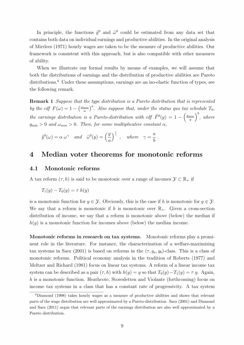
Figure 7: Sufficient statistics for Pareto-improving, Politically feasible, and Welfare-
improving tax reforms
or
T ′0(y0) > DWg (y0) and T ′0(y0) > DM(y0) . (14)
Proposition 8 states sufficient conditions for the existence of welfare-improving and
politically feasible reforms. This raises the question of necessary conditions. Proposition
8 has been derived from focussing on “small” reforms, i.e., on small increases of marginal
tax rates applied to a small range of incomes. The arguments in the proofs of Propositions
4 - 7 imply that if either condition (13) or condition (14) is violated at y0, then there
is no small reform in the (τ, ya, yb)-class that is both welfare-improving and politically
feasible.
y
T ′0 =T ′0
1−T ′0
DM
DWg
Figure 8: Sufficient statistics for politically feasible reforms and welfare-improving reforms
with a laissez-faire status quo schedule
26

Figure 8 provides an illustration under the assumptions that the status quo schedule
is the laissez-faire schedule.12 The figure shows that for incomes above the median, an
increase in marginal tax rates is both welfare-improving and politically feasible. This
holds for any welfare function under which the function g is strictly decreasing.13 By
contrast, for incomes below the median, there is no reform that is both politically feasible
and welfare-improving: welfare improvements require to raise marginal taxes relative to
the laissez-faire ones, whereas political feasibility requires to introduce negative marginal
tax rates.
For Figure 7 (right panel), the status quo tax schedule is, again, as in (10). In this
example, for high incomes, tax rates are inefficiently high so that tax cuts are both
politically feasible and welfare-improving. There is a range of incomes above the median
income where tax cuts are not mandated by Pareto-efficiency. In this region, tax increases
are therefore politically feasible. They are, however, not desirable for the given welfare
function. For a range of incomes below the median income, tax cuts are politically
feasible and welfare-improving. For low incomes, tax cuts are politically feasible, but
welfare-damaging.
Our analysis in this section provides a diagnosis system that can be used to identify
reform options that are associated with a given income tax system. In particular, we can
check wether there is scope for revenue increases, Pareto-improvements, welfare improve-
ments and, moreover, for reforms that are politically feasible in the sense that they make
a majority of individuals better off.
The analysis suggests that existing tax schedules might be viewed as resulting from
a compromise between concerns for welfare-maximization on the one hand, and concerns
for political support on the other. If the maximization of political support was the only
force in the determination of tax policy, we would expect to see tax rates close to the
revenue-maximizing rate DR for incomes above the median and negative rates close to
DP for incomes below the median. Concerns for welfare dampen these effects. A welfare-
maximizing approach will generally yield higher marginal tax rates for incomes below the
median and lower marginal tax rates for incomes above the median.
Our analysis also raises a question. Diamond (1998) and Saez (2001) have argued
that, for plausible specifications of welfare weights, existing tax schedules have marginal
tax rates for high incomes that are too low. Our analysis would suggest that an increase
of these tax rates would not only be welfare-improving but also politically feasible. Why
don’t we see more reforms that involve higher tax rates for the rich? Proposition 1
provides a possible answer to this question: reforms that do not belong to the (τ, ya, yb)-
class but instead involve tax cuts that are larger for richer taxpayers may as well prove
to be politically feasible. For such reforms political feasibility requires that the median
12A reform of a laissez-faire status quo schedule corresponds to the introduction of an income tax
schedule as studied in Aidt and Jensen (2009).13If g(ω) = 1, for all ω, then such tax increases are politically feasible, but not welfare improving.
27
voter is included in the set of those who benefit from the tax cuts.
6 Extensions
In this section we show that the median voter theorem for small monotonic reforms (The-
orem 1) applies to models with more than one source of heterogeneity among individuals.
Again, we show that a small tax reform is preferred by a majority of taxpayers if and
only if it is preferred by the taxpayer with median income. Throughout, we stick to the
assumption that individuals differ in their productive abilities ω. We introduce a second
consumption good and the possibility of heterogeneity in preferences over consumption
goods in Section 6.1. We use this framework to discuss whether the introduction of dis-
tortionary taxes on savings is politically feasible. In Section 6.2 we consider fixed costs of
labor market participation as an additional source of heterogeneity.14 In Section 6.3 we
assume that individuals differ in their valuation of increased public spending.15 Finally,
in Section 6.4, individuals differ by how much of their income is due to luck as in Alesina
and Angeletos (2005).
6.1 Political support for taxes on savings
We now suppose that there are two consumption goods. We refer to them as food and
savings, respectively. An individual’s budget constraint now reads as
cf + cs + T0s(cs) + τshs(cs) ≤ c0 + y − T0(y)− τh(y) . (15)
The variables on the right-hand side of the budget constraint have been defined before.
On the left-hand side, cf denotes food consumption and cs savings. In the status quo
savings are taxed according to a possibly non-linear savings-tax function T0s. A reform
replaces both the status quo income tax schedule T0 by T1 = T0 + τh and the status
quo savings tax schedule T0s by T1s = T0s + τshs. We maintain the assumption that the
functions h and hs are non-decreasing and focus on revenue neutral reforms so that either
τ > 0 and τs < 0 or τ < 0 and τs > 0.
Preferences of individuals are given by a utility function u(v(cf , cs, β), y, ω), where v is
a subutility function that assigns consumption utility to any consumption bundle (cf , cs).
The marginal rate of substitution between food and savings depends on a parameter β.
We do not assume a priori that β is the same for all individuals. Under this assumption,
however, the utility function u has the properties under which an efficient tax system
does not involve distortionary commodity taxes, see Atkinson-Stiglitz (1976), or Laroque
(2005) for a more elementary proof. Distortionary taxes on savings are then undesirable
from a welfare-perspective.
14See Saez (2002), Chone and Laroque (2011), and Jacquet, Lehmann and Van der Linden (2013).15See Boadway and Keen (1993), Hellwig (2004), Bierbrauer and Sahm (2010), Bierbrauer (2014), or
Weinzierl (forthcoming).
28

Individuals choose cf , cs and y to maximize utility subject to the budget constraint
above. We denote the utility maximizing choices by c∗f (τs, τ, β, ω), c∗s(τs, τ, β, ω) and
y∗(τs, τ, β, ω) and the corresponding level of indirect utility by V (τs, τ, β, ω). The slope of
an indifference curve in a τ -τs diagram determines the individuals’ willingness to accept
higher savings taxes in return for lower taxes on current earnings. The following Lemma
provides a characterization of this marginal rate of substitution in a neighborhood of the
status quo. Let
s(τ, τ s, β, ω) = − Vτ (τs, τ, β, ω)
Vτs(τs, τ, β, ω)
be the slope of an individual’s indifference curve in a τ -τs diagram. The slope in the
status quo is denoted by s0(ω, β). We denote the individual’s food consumption, savings
and earnings in the status quo by c0f (ω, β), c0
s(ω, β) and y0(ω, β), respectively.
Lemma 4 In the status quo the slope of a type (ω, β)-individual’s indifference curve in
a τ -τs diagram is given by
s0(ω, β) = − h(y0(ω, β))
hs(c0s(ω, β))
.
The proof of Lemma 4 can be found in the Appendix. The Lemma provides a gener-
alization of Roy’s identity that is useful for an analysis of non-linear tax systems. As
is well known, with linear tax systems, the marginal effect of, say, an increased savings
tax on indirect utility is equal to −λ∗c∗s(·), where λ∗ is the multiplier on the individual’s
budget constraint, also referred to as the marginal utility of income. Analogously, the
increase of a linear income tax affects indirect utility via −λ∗y∗(·) so that the slope of an
indifference curve in a τs-τ -diagram would be equal to the earnings-savings-ratio −y∗(·)c∗s(·) .
Allowing for non-linear tax systems and non-linear perturbations implies that the simple
earnings-savings-ratio is replaced by − h(y∗(·))hs(c∗s(·)) .
Consider a reform that involves an increase in the savings tax rate dτs > 0 and a
reduction of taxes on income dτ < 0. We say that a type (ω, β)-individual strictly prefers
a small reform with increased savings taxes over the status quo if
Vτs(0, 0, β, ω) dτs + Vτ (0, 0, β, ω) dτ > 0 ,
or, equivalently, if
dτsdτ
> s0(ω, β) = − h(y0(ω, β))
hs(c0s(ω, β))
. (16)
Since hs is an increasing function, this condition is, ceteris paribus, easier to satisfy
if the individual has little savings in the status quo. The ratio dτsdτ
on the left-hand
side of inequality (16) follows from the behavioral responses of individuals to a small
revenue-neutral tax reform. Let ∆Rs(τs, τ) be the change of revenue from savings taxes
29

and ∆R(τs, τ) the change of revenue from income taxation due to the reform. Revenue-
neutrality requires that
∆Rsτs (τs, τ)d τs + ∆Rs
τ (τs, τ) dτ + ∆Rτs(τs, τ) dτs + ∆R
τ (τs, τ) dτ = 0 ,
or, equivalently, that
dτsdτ
= −∆Rτ (τs, τ) + ∆Rs
τ (τs, τ)
∆Rsτs (τs, τ) + ∆R
τs(τs, τ),
which has to be evaluated for (τs, τ) = (0, 0). We simply assume that, for the reforms
that we consider, this expression is well-defined and takes a finite negative value.
Different types will typically differ in their generalized earnings-savings-ratio s0(ω, β)
and we can order types according to this one-dimensional index. Let (ω, β)0M be the
type with the median value of s0(ω, β). The following proposition extends Theorem 1.
It asserts that a small reform is politically feasible if and only if it is supported by the
median type (ω, β)0M .
Proposition 9 For a given status quo tax policy and a given pair of non-decreasing
functions h and hs, the following statements are equivalent:
1. Type (ω, β)0M prefers a small reform with increased savings taxes over the status
quo.
2. There is a majority of individuals who prefer a small reform with increased savings
taxes over the status quo.
As Theorem 1, Proposition 9 exploits the observation that individuals can be ordered
according to a one-dimensional statistic that pins down whether or not they benefit from
a tax reform. This makes it possible to prove a median-voter theorem for reforms that
remain in a neighborhood of the status quo. There is also a difference to Theorem 1.
With only one-dimensional heterogeneity, there is a monotonic relation between types
and earnings so that the identity of the type with median income does not depend on
the status quo. Whatever the tax system, the person with the median income is the
person with the median type ωM . Here, by contrast, we allow for heterogeneity both
in productive abilities and in preferences over consumption goods. The type with the
median value of the generalized earnings-savings-ratio s0(ω, β) will then typically depend
on the status quo tax system. This does not pose a problem if we focus on small reforms.
In this case, preferences over reforms follow from the generalized earnings-savings-ratios
in the status quo, and a small reform is preferred by a majority of individuals if and only
if it is preferred by the individual with the median ratio.
30
6.2 Fixed costs of labor market participation
With fixed costs of labor market participation individuals derive utility u(c−θ 1y>0, y, ω)
from a (c, y)-pair. Fixed costs θ absorb some of the individual’s after-tax income if the
individual becomes active on the labor market, e.g. because of additional child care
expenses. As before, there is an initial status quo tax schedule under which earnings are
transformed into after-tax income according to the schedule C0 with C0(y) = c0+y−T0(y).
After a reform, the schedule is
C1(y) = c0 + ∆R + y − T0(y)− τ h(y) ,
where h is a non-decreasing function of y. We denote by y∗(∆R, τ, ω, θ) the solution to
maxy
u(C1(y)− θ 1y>0, y, ω),
and the corresponding level of indirect utility by V (∆R, τ, ω, θ). We proceed analogously
for other variables: what has been a function of ω in previous sections is now a function
of ω and θ.
For a given function h, the marginal gain that is realized by an individual with type
(ω, θ) if the tax rate τ is increased, is given by the following analogue to equation (4),
∆Vτ (ω, θ | τ, h) = u1
c(ω, θ)(∆Rτ (τ, h)− h(y1(ω, θ))
), (17)
where u1c(ω, θ) is the marginal utility of consumption realized by a type (ω, θ)-individual
after the reform, and y1(ω, θ) are the individual’s post-reform earnings. At τ = 0, we can
also write
∆Vτ (ω, θ | 0, h) = u0
c(ω, θ)(∆Rτ (0, h)− h(y0(ω, θ))
), (18)
where u0c(ω, θ) and y0(ω, θ) are, respectively, marginal utility of consumption and earnings
in the status quo.
For a given status quo tax policy and a given function h we say that type (ω, θ)
strictly prefers a small tax reform over the status quo if ∆Vτ (ω, θ | 0, h) > 0. The
status quo median voter strictly prefers a small reform if ∆Vτ
((ω, θ)0M | 0, h
)> 0, where
y0M is the median of the distribution of earnings in the status quo and (ω, θ)0M is the
corresponding type; i.e. y0((ω, θ)0M
)= y0M .
Proposition 10 For a given status quo tax policy and a monotonic function h, the fol-
lowing statements are equivalent:
1. Type (ω, θ)0M prefers a small reform over the status quo.
2. There is a majority of individuals who prefer a small reform over the status quo.
31

Proposition 10 exploits that the slope of a type (ω, θ) individual’s indifference curve
through a point (τ,∆R),
s(τ,∆R, ω, θ) = h(y∗(∆R, τ, ω, θ)) .
is a function of the individual’s income. As in the basic Mirrleesian setup, the inter-
pretation is that individuals with a higher income are more difficult to convince that a
reform that involves tax increases (τ > 0) is worthwhile. A difference to the Mirrleesian
setup is, however, that there is no monotonic relation between types and earnings. In
the presence of income effects, and for a given level of ω, y∗ will increase in θ as long
as θ is below a threshold θ(ω) and be equal to 0 for θ above the threshold. This also
implies that there is no longer a fixed type whose income is equal to the median income
whatever the tax schedule. As in Proposition 9, this does not pose a problem if we focus
on small reforms, i.e. on small deviations from (τ,∆R) = (0, 0). In this case, preferences
over reforms follow from the relation between types and earnings in the status quo, and
a small reform is preferred by a majority of individuals if and only if it is preferred by
the individual with the median level of income in the status quo.
6.3 Public-goods preferences
Suppose that the change in revenue ∆R is used to increase or decrease spending on
publicly provided goods. The post-reform consumption schedule is then given by
C1(y) = c0 + y − T0(y)− τ h(y) ,
We assume that individuals differ with respect to their public-goods preferences. Now
the parameter θ is a measure of an individual’s willingness to give up private goods con-
sumption in exchange for more public goods. More specifically, we assume that individual
utility is
u(θ(R0 + ∆R) + C1(y), y, ω) ,
where R0 is spending on publicly provided goods in the status quo. Again, we denote by
y∗(∆R, τ, ω, θ) the solution to
maxy
u(θ(R0 + ∆R) + C1(y), y, ω)
and indirect utility by V (∆R, τ, ω, θ). By the envelope theorem, the slope of a type (ω, θ)
individual’s indifference curve through point (τ,∆R) is now given by
s(τ,∆R, ω, θ) =h(y∗(∆R, τ, ω, θ))
θ.
This marginal rate of substitution gives the increase in public-goods provision that an
individual requires as a compensation for an increase of marginal tax rates. Ceteris
paribus, individuals with a lower income and individuals with a higher public-goods
32

preference require less of a compensation, i.e. they have a higher willingness to pay higher
taxes for increased public-goods provision. If we focus on small reforms we observe, again,
that if a type (ω, θ)-individual benefits from a small tax-increase, then the same is true
for any type (ω′, θ′) with
h(y0(ω, θ))
θ≥ h(y0(ω′, θ′))
θ′.
By the arguments in the proof of Proposition 10, a small reform with τ > 0 is preferred
by a majority of individuals if and only if(h(y0(ω, θ))
θ
)0M
<d∆R
dτ,
where(h(y0(ω,θ))
θ
)0M
is the median willingness to pay higher taxes for increased public
spending in the status quo.
6.4 Fairness and politically feasible reforms
We analyze politically feasible reforms of non-linear tax systems for a setup in which
individual incomes can be due to luck or effort and in which preferences over reforms
include a motive to tax income that is due to luck more heavily than income that is due
to effort. In modeling such preferences we adopt the framework of Alesina and Angeletos
(2005). Alesina and Angeletos focus, however, on linear tax systems.
There are two periods. When young individuals choose a level of human capital
k. When old individuals choose productive effort or labor supply l. Pre-tax income is
determined by
y = π(l, k) + η ,
where π is a production function that is increasing in both arguments and η is a random
source of income, also referred to as luck. An individual’s life-time utility is written as
u(c, l, k, ω). Utility is increasing in the first argument. It is decreasing in the second and
third argument to capture the effort costs of labor supply and human capital investments,
respectively. Effort costs are decreasing in ω. More formally, lower types have steeper
indifference curves both in a (c, l)-space and in a (c, k)-space. We consider reforms that
lead to a consumption schedule
C1(y) = c0 + ∆R + y − T0(y)− τ h(y) .
We assume that individuals first observe how lucky they are and then choose how hard
they work, i.e. given a realization of η and given the predetermined level of k, individuals
choose l so as to maximize
u(C1(π(l, k) + η), l, k, ω) .
33

We denote the solution to this problem by l∗(∆R, τ, ω, η, k). Indirect utility is denoted by
V (∆R, τ, ω, η, k). As of t = 1, there is multi-dimensional heterogeneity among individuals:
they differ in their type ω, in their realization of luck η and possibly also in their human
capital k.
In Alesina and Angeletos (2005) preferences over reforms have a selfish and fairness
component. The indirect utility function V shapes the individuals’ selfish preferences
over reforms, for predetermined levels of human capital. The analysis of these selfish
preferences can proceed along similar lines as the extension that considered fixed costs of
labor market participation. Selfish preferences over small reforms follow from the relation
between types and earnings in the status quo, and a small reform makes a majority better
off if and only if it is beneficial for the individual with the median level of income in
the status quo. More formally, let y0(ω, η, k) := y∗(0, 0, ω, η, k) be a shorthand for the
earnings of a type (ω, η, k)-individual in the status quo and recall that the sign of
s(0, 0, ω, η, k) = h(y0(ω, η, k))
determines whether an individual benefits from a small tax reform. Specifically, suppose
that h is a non-decreasing function and denote by y0M the median level of income in
the status quo and by (ω, η, k)0M the corresponding type. A majority of individuals is –
according to their selfish preferences – made better off by reform if and only if the median
voter benefits from the reform,
s0((ω, η, k)0M
)= h
(y0M
)<d∆R
dτ.
In their formalization of social preferences, Alesina and Angeletos (2005) view π(l, k)
as a reference income. It is the part of income that is due to effort as opposed to luck. A
tax reform affects the share of y = π(l, k) + η that individuals can keep for themselves.
After the reform, the difference between disposable income and the reference income is
given by16
C1(y)− π(l, k) = η − T0(π(l, k) + η)− τh(π(l, k) + η) .
A social preferences for fair taxes is then equated with a desire to minimize the variance
of η − T0(π(l, k) + η) − τh(π(l, k) + η) taking into account that k and l are endogenous
variables.17 Denote this variance henceforth by Σ(∆R, τ). Any one individual is assumed
to evaluate a tax reform according to
V (∆R, τ, ω, η, k)− ρ Σ(∆R, τ) ,
16The analysis in Alesina and Angeletos (2005) looks at a special case of this. They focus on a status
quo equal to the laissez-faire schedule so that T0(y) = 0, for all y, and a reform that introduces a linear tax
schedule, i.e. h(y) = y, for all y. Under these assumptions, we have η−T0(π(l, k)+η)−τh(π(l, k)+η) =
(1− τ)η + τπ(l, k) .17Human capital investment is a function of effort costs ω and the expectations (∆Re, τe) of the young
on the tax reforms that will be adopted when they are old.
34

where ρ is the weight on fairness considerations which is assumed to be the same for
all individuals. Therefore, heterogeneity in preferences over reforms is entirely due to
heterogeneity in selfish preferences. Consequently, the finding that a small reform is
preferred by a majority of taxpayers if and only if it is preferred by the voter with
median income in the status quo is not affected by the inclusion of a demand for fair
taxes.
7 Concluding remarks
This paper develops a framework for an analysis of tax reforms. This framework can
be applied to any given income tax system. It makes it possible to identify reforms
that are politically feasible in the sense that they would be supported by a majority of
taxpayers or to identify welfare-improving reforms. One can also study the intersection
of politically feasible and welfare-improving reforms. If this set is empty, the status quo
is constrained efficient because the scope for politically feasible welfare-improvements has
been exhausted.
With non-linear tax systems, the policy-space is multi-dimensional with the impli-
cation that political economy forces are difficult to characterize. A main result in our
paper is that this difficulty can be overcome by looking at tax reforms that are monotonic
such that the change in tax payments is a monotonic function of income. We show that,
with such a policy space, a reform is preferred by a majority of taxpayers if and only if
it is preferred by the taxpayer with median income. This implies that tax decreases for
incomes below the median and tax increases for incomes above the median are politically
feasible, provided that tax rates stay within Pareto bounds.
Our analysis identifies, for each level of income, Pareto-bounds for marginal tax rates.
It also identifies reforms that would be preferred by a majority of voters. Moreover,
we derive sufficient statistics that make it possible to bring this framework to the data.
This allows to diagnose what types of reforms are possible under a given status quo tax
policy. Future research might use this framework to complement existing studies on the
history of income taxation. For instance, Scheve and Stasavage (2016) study whether
tax systems have become more progressive in response to increases in inequality or in
response to extensions of the franchise. Their analysis compares tax policies that have
been adopted at different points in time, or by countries with different institutions. It
does not include an analysis of the reforms that appear to have been politically feasible or
welfare-improving in a given year for a given country and a given status quo tax schedule.
The framework that is developed in this paper lends itself to such an analysis.
Finally, we develop our analysis mainly in the context of a Mirrleesian model of in-
come taxation in which individuals differ in their costs of effort. A similar analysis would
be possible for any model of taxation in which a version of the Spence-Mirrlees single
crossing property holds. We also show that our analysis of small monotonic reforms ex-
35

tends to models with multi-dimensional heterogeneity of individuals, such as models with
variable and fixed costs of labor market participation, models that include heterogeneity
in preferences over public goods, or models that include an investment in human capital.
References
Acemoglu, D., M. Golosov, and A. Tsyvinski, “Political Economy of Mechanisms,”
Econometrica, 2008, 76, 619–641.
, , and , “Dynamic Mirrlees Taxation under Political Economy Con-
straints,” Review of Economic Studies, 2010, 77, 841–881.
, S. Naidu, P. Restrepo, and J.A. Robinson, “Democracy, Redistribution, and
Inequality,” Handbook of Income Distribution, 2015, pp. 1885–1966.
Aidt, T.S. and P.S. Jensen, “The taxman tools up: An event history study of the
introduction of the personal income tax,” Journal of Public Economics, 2009, 93 (1),
160–175.
Alesina, A. and G.-M. Angeletos, “Fairness and Redistribution,” American Eco-
nomic Review, 2005, 95 (4), 960–980.
, S. Stantcheva, and E. Teso, “Intergenerational Mobility and Support for Re-
distribution,” NBER Working Paper 23027, 2017.
Atkinson, A. and J. Stiglitz, “The Design of Tax Structure: Direct versus Indirect
Taxation,” Journal of Public Economics, 1976, 1, 55–75.
Bargain, O., M. Dolls, D. Neumann, A. Peichl, and S. Siegloch, “Tax-Benefit
Systems in Europe and the US: Between Equity and Efficiency,” IZA Discussion
Papers 5440, 2011.
Baron, D. and J. Ferejohn, “Bargaining in Legislatures,” American Political Science
Review, 1989, 83, 1181–1206.
Barro, R., “The Control of Politicians: An economic model,” Public Choice, 1973, 14,
19–42.
Bastani, S. and J. Lundberg, “Political preferences for redistribution in Sweden,”
Working Paper, 2016.
Battaglini, M. and S. Coate, “A Dynamic Theory of Public Spending, Taxation and
Debt,” American Economic Review, 2008, 98, 201–236.
Benabou, R. and E.A. Ok, “Social Mobility and the Demand for Redistribution: The
Poum Hypothesis,” Quarterly Journal of Economics, 2001, 116 (2), 447–487.
36

and J. Tirole, “Belief in a just world and redistributive politics,” Quarterly Journal
of Economics, 2006, 121 (2), 699–746.
Bierbrauer, F.J., “Optimal Tax and Expenditure Policy with Aggregate Uncertainty,”
American Economic Journal: Microeconomics, 2014, 6 (1), 205–57.
and M. Sahm, “Optimal democratic mechanisms for taxation and public good
provision,” Journal of Public Economics, 2010, 94 (78), 453 – 466.
and P.C. Boyer, “Efficiency, Welfare, and Political Competition,” Quarterly Jour-
nal of Economics, 2016, 131 (1), 461–518.
Black, D., “On the Rationale of Group Decision-making,” Journal of Political Economy,
1948, 56 (1), 23–34.
Blundell, R., M. Brewer, P. Haan, and A. Shephard, “Optimal income taxation of
lone mothers: an empirical comparison of the UK and Germany,” Economic Journal,
2009, 119, F101–F121.
Boadway, R. and M. Keen, “Public Goods, Self-Selection and Optimal Income Tax-
ation,” International Economic Review, 1993, 34, 463–478.
Bourguignon, F. and A. Spadaro, “Tax-benefit Revealed Social Preferences,” Journal
of Economic Inequality, 2012, 10 (1), 75–108.
Brett, C. and J.A. Weymark, “Voting over selfishly optimal nonlinear income tax
schedules with a minimum-utility constraint,” Journal of Mathematical Economics,
2016, 67, 18–31.
and , “Voting over selfishly optimal nonlinear income tax schedules,” Games
and Economic Behavior, 2017, 101, 172–188.
Chone, P. and G. Laroque, “Optimal taxation in the extensive model,” Journal of
Economic Theory, 2011, 146 (2), 425–453.
Christiansen, V. and E. Jansen, “Implicit Social Preferences in the Norwegian System
of Indirect Taxation,” Journal of Public Economics, 1978, 10 (2), 217–245.
Diamond, P.A., “Optimal Income Taxation: An Example with a U-Shaped Pattern of
Optimal Marginal Tax Rates,” American Economic Review, 1998, 88, 83–95.
and E. Saez, “The Case for a Progressive Tax: From Basic Research to Policy
Recommendations,” Journal of Economic Perspectives, 2011, 25 (4), 165–90.
Drazen, A., Political Economy in Macroeconomics, Princeton University Press, 2000.
37

Farhi, E., C. Sleet, I. Werning, and S. Yeltekin, “Non-linear Capital Taxation
Without Commitment,” Review of Economic Studies, 2012, 79 (4), 1469–1493.
Feldstein, Martin, “On the theory of tax reform,” Journal of Public Economics, 1976,
6 (12), 77 – 104.
Ferejohn, J., “Incumbent Performance and Electoral Control,” Public Choice, 1986, 50,
5–25.
Gans, J.S. and M. Smart, “Majority voting with single-crossing preferences,” Journal
of Public Economics, 1996, 59 (2), 219 – 237.
Golosov, M., A. Tsyvinski, and N. Werquin, “A Variational Approach to the
Analysis of Tax Systems,” Working Paper 20780, National Bureau of Economic
Research December 2014.
Guesnerie, R., A Contribution to the Pure Theory of Taxation, Cambridge University
Press, 1995.
Heathcote, J., K. Storesletten, and G.L. Violante, “Optimal Tax Progressivity:
An Analytical Framework,” Quarterly Journal of Economics, forthcoming.
Hellwig, M.F., “Optimal income taxation, public-goods provision and public-sector
pricing: A contribution to the foundations of public economics,” MPI Collective
Goods Preprint, 2004, 2004/14.
, “A Contribution to the Theory of Optimal Utilitarian Income Taxation,” Journal
of Public Economics, 2007, 91, 1449–1477.
Hendren, N., “The Inequality Deflator: Interpersonal Comparisons without a Social
Welfare Function,” NBER Working Paper 20351, 2014.
Ilzetzki, E., “A positive theory of tax reform,” Mimeo, London School of Economics,
2015.
Jacquet, L. and E. Lehmann, “Optimal Taxation with Heterogeneous Skills and Elas-
ticities: Structural and Sufficient Statistics Approaches,” THEMA Working Paper
2016/04, 2016.
, , and B. Van der Linden, “Optimal redistributive taxation with both
extensive and intensive responses,” Journal of Economic Theory, 2013, 148 (5),
1770 – 1805.
Kleven, H.J., “Bunching,” Annual Review of Economics, 2016, 8, 435–464.
Laroque, G., “Indirect taxation is superfluous under separability and taste homogeneity:
a simple proof,” Economic Letters, 2005, 87, 141–144.
38

Lindbeck, A. and J. Weibull, “Balanced-budget Redistribution as the Outcome of
Political Competition,” Public Choice, 1987, 52, 273–297.
Lockwood, B.B. and M. Weinzierl, “Positive and normative judgments implicit in
U.S. tax policy, and the costs of unequal growth and recessions,” Journal of Monetary
Economics, 2016, 14-119 (77), 30–47.
Meltzer, A. and S. Richard, “A Rational Theory of the Size of Government,” Journal
of Political Economy, 1981, 89, 914–927.
Mirrlees, J., “An Exploration in the Theory of Optimum Income Taxation,” Review of
Economic Studies, 1971, 38, 175–208.
Myerson, R., “Incentives to Cultivate Favored Minorities Under Alternative Electoral
Systems,” American Political Science Review, 1993, 87 (4), 856–869.
Peichl, A., N. Pestel, S. Siegloch, and E. Sommer, “Bundestagswahlkampf 2013:
Klientelpolitik durch Steuerreform?.,” Perspektiven der Wirtschaftspolitik, 2014, 15
(2), 182–194.
Persson, T and G. Tabellini, Political Economics: Explaining Economic Policy, Cam-
bridge, MA, MIT Press, 2000.
Piketty, T., “Social mobility and redistributive politics,” Quarterly Journal of Eco-
nomics, 1995, 110 (3), 551–584.
, “La redistribution fiscale face au chomage,” Revue francaise d’economie, 1997, 12,
157–201.
and E. Saez, “Optimal Labor Income Taxation,” Handbook of Public Economics,
2013, pp. 391–474.
Roell, A.A., “Voting over Nonlinear Income Tax Schedules,” Working Paper, 2012.
Roberts, K., “Voting over Income Tax Schedules,” Journal of Public Economics, 1977,
8.
Rothstein, P., “Order restricted preferences and majority rule,” Social Choice and
Welfare, 1990, 7 (4), 331–342.
, “Representative Voter Theorems,” Public Choice, 1991, 72 (2/3), 193–212.
Saez, E., “Using Elasticities to Derive Optimal Income Tax Rates,” Review of Economic
Studies, 2001, 68, 205–229.
, “Optimal Income Transfer Programs: Intensive versus Extensive Labor Supply
Responses,” Quarterly Journal of Economics, 2002, 117 (3), 1039–1073.
39
, “Do Taxpayers Bunch at Kink Points?,” American Economic Journal: Economic
Policy, August 2010, 2 (3), 180–212.
and S. Stantcheva, “Generalized Social Marginal Welfare Weights for Optimal
Tax Theory,” American Economic Review, 2016, 106 (1), 24–45.
Scheuer, F. and A. Wolitzky, “Capital taxation under political constraints,” Ameri-
can Economic Review, 2016, 106 (8), 2304–2328.
and I. Werning, “Mirrlees meets Diamond-Mirrlees,” Working Paper 22076, Na-
tional Bureau of Economic Research 2016.
Scheve, K. and D. Stasavage, Taxing the Rich: A History of Fiscal Fairness in the
United States and Europe, Princeton University Press, 2016.
Seade, J., “On the Sign of the Optimum Marginal Income Tax,” Review of Economic
Studies, 1982, 49 (4), 637–643.
Sheshinski, E., “The Optimal Linear Income-tax,” Review of Economic Studies, 1972,
39, 297–302.
Weinzierl, M., “Revisiting the classical view of benefit-based taxation,” Economic Jour-
nal, forthcoming.
Weymark, John A., “Undominated directions of tax reform,” Journal of Public Eco-
nomics, 1981, 16 (3), 343 – 369.
Zoutman, F.T., B. Jacobs, and E.L.W. Jongen, “Optimal Redistributive Taxes
and Redistributive Preferences in the Netherlands,” mimeo: Erasmus University
Rotterdam/CPB Netherlands Bureau for Economic Policy Research, 2014.
, , and , “Redistributive Politics and the Tyranny of the Middle Class,”
Tinbergen Institute Discussion Paper 16-032/VI, 2016.
40

Appendix
A Reforms in the (τ, ya, yb)-class: Behavioral responses
Reforms in the (τ, ya, yb)-class involve jumps of marginal tax rates at ya and yb. Lemmas A.1-A.3
below clarify the behavioral responses to these discontinuities. Figure 9 provides an illustration.
y
c
C1(y)
C0(y)
c0 + ∆R
c0
c0 + ∆R − τ(yb − ya)
ya yb
IC1a
IC2a
IC0a
IC1b
IC2b
IC0b
Figure 9:The figure depicts the following curves:
(a) C0(y) = c0 + y − T0(y), C1(y) = c0 + ∆R
+ y − T0(y)− τh(y),
(b) IC0b indifference curve of type ωb(0) through yb under C0(y), IC1
b curve through yb under C1(y) when there are no income effects, IC2b
curve through yb under C1(y) with income effects;
(c) IC0a indifference curve of type ωa(0) through ya under C0(y), IC1
a curve through ya under C1(y) when there are no income effects,
IC2a curve through ya under C1(y) if there are income effects.
The Spence-Mirrlees single crossing property implies that, under any tax schedule, more
productive individuals choose a higher level of pre-tax income. Thus, ω′ > ω implies that
y∗(∆R(τ ′, ya, yb), τ′, ω′) ≥ y∗(∆R(τ ′, ya, yb), τ
′, ω) ,
for τ ′ ∈ 0, τ. We can therefore define threshold types ωa(τ′) and ωb(τ
′) so that
ω ≤ ωa(τ ′) implies y∗(∆R(τ ′, ya, yb), τ′, ω) ≤ ya ,
ω ∈ (ωa(τ′), ωb(τ
′)) implies y∗(∆R(τ ′, ya, yb), τ′, ω) ∈ (ya, yb) ,
41

and
ω ≥ ωb(τ ′) implies y∗(∆R(τ ′, ya, yb), τ′, ω) ≥ yb .
The following Lemma asserts that, for a reform that involves an increase of the marginal
tax rate, τ > 0, type ωa(0) who chooses an income of ya before the reform does not choose a
level of income above ya after the reform. Analogously, if marginal taxes go down, type ωb(0)
does not choose an income above yb after the reform. For a reform with τ > 0, the logic is as
follows: After the reform, because of the transfer ∆R, a type ωa(0)-individual is, at income level
ya, less eager to work more. Working more also is less attractive after the reform because of the
increased marginal tax rates for incomes above ya. Thus, both the income and the substitution
effect associated with the reform make it less attractive for a type ωa(0)-individual to increase
her income above ya. The individual will therefore either stay at ya or decrease her income after
the reform. Only higher types will end up with an income of ya after the reform, which implies
ωa(0) ≤ ωa(τ).
Lemma A.1
1. Consider a reform so that τ > 0 and ∆R(τ, ya, yb) > 0. Then ωa(τ) ≥ ωa(0).
2. Consider a reform so that τ < 0 and ∆R(τ, ya, yb) < 0. Then ωb(τ) ≥ ωb(0).
Proof We only prove the first statement. The proof of the second statement follows from an
analogous argument. Under the initial tax schedule T0 an individual with type ωa(0) prefers
ya over all income levels y ≥ ya. We argue that the same is true under the new tax schedule
T1. This proves that ωa(τ) ≥ ωa(0). Consider a y-c-diagram and the indifference curve of
a type wa(0)-type through the point (ya, c0 + ya − T0(ya)). By definition of type wa(0), all
points (y, y−T0(y)) with y > ya lie below this indifference curve under the initial tax schedule.
Under the new schedule T1, this individual receives a lump-sum transfer ∆R > 0. Hence, the
indifference curve through (ya, c0 + ∆R + ya − T0(ya)) is at least as steep as the indifference
curve through (ya, c0 + ya − T0(ya)). Thus, the individual prefers (ya, c0 + ∆R + ya − T0(ya))
over all points (y, c0 + ∆R + y − T0(y)) with y > ya. Since for all y > ya, T1(y) > T0(y), the
individual also prefers (ya, c0 + ∆R + ya − T0(ya)) over all points (y, c0 + ∆R + y − T1(y)) with
y > ya.
According to the next lemma a reform induces bunching of individuals who face an upward
jump of marginal tax rates after the reform. Specifically, a reform with τ > 0 will induce
bunching at ya because marginal tax rates jump upwards at income level ya. A reform with
τ < 0 will induce bunching at yb because marginal tax rates jump upwards at income level yb.
Lemma A.2
1. Consider a reform so that τ > 0 and ∆R(τ, ya, yb) > 0. Then there is a set of types
[ωa(τ), ωa(τ)] who bunch at ya after the reform.
2. Consider a reform so that τ < 0 and ∆R(τ, ya, yb) < 0. Then there is a set of types
[ωb(τ), ωb(τ)] who bunch at yb after the reform.
42

Proof Consider a reform that involves an increase of marginal tax rates τ > 0. If before the
reform, all types where choosing an income level y∗(0, 0, ω) that satisfies the first order condition
uc(·)(1− T ′0(·)) + uy(·) = 0 ,
then, after the reform there will be a set of types (ωa(τ), ω(τ)] who will now bunch at ya. These
individuals chose an income level above ya before the reform. After the reform they will find
that
uc(·)(1− T ′0(·)− τ) + uy(·) < 0 ,
for all y ∈ (ya, y∗(0, 0, ω)] and therefore prefer ya over any income in this range. At the same
time, they will find that
uc(·)(1− T ′0(·)) + uy(·) > 0 ,
so that there is also no incentive to choose an income level lower than ya. Hence, the types who
bunch are those for which at ya,
1− T ′0(ya) > −uy(·)uc(·)
> 1− T ′0(ya)− τ .
An analogous argument implies that for a reform that involves a decrease in marginal tax rates
τ > 0, there will be a set of types [ωb(τ), ωb(τ)] who bunch at yb after the reform.
Individuals who bunch at ya after a reform with τ > 0 neither have an incentive to increase
their earnings above ya since
uc(·)(1− T ′1(ya)) + uy(·) = uc(·)(1− T ′0(ya)− τ) + uy(·) ≤ 0
nor an incentive to lower their earnings since
uc(·)(1− T ′0(ya)) + uy(·) ≥ 0 .
By contrast, there are no individuals who bunch at yb after a reform that involves increased
marginal tax rates. Individuals who do not have an incentive to increase their income at yb
since
uc(·)(1− T ′1(yb)) + uy(·) = uc(·)(1− T ′0(yb)) + uy(·) ≤ 0
definitely have an incentive to lower their income as
uc(·)(1− T ′0(yb)− τ) + uy(·) < 0 .
An analogous argument implies that no one will bunch at ya after a reform that involves a
decrease of marginal tax rates.
The next Lemma establishes that, in the absence of income effects, for a reform with τ > 0,
individuals who choose an income above yb after the reform also chose an income above yb before
the reform. This ordering is reversed for a reform with τ < 0. We will subsequently discuss
why these statements need no longer be true if there are income effects.
43

Lemma A.3 Suppose that there are no income effects, i.e. for all (c, y, ω) and any pair (e, e′)
with e′ > e,
−uy(c+ e, y, ω′)
uc(c+ e, y, ω′)= −uy(c+ e′, y, ω)
uc(c+ e′, y, ω).
1. Consider a reform so that τ > 0 and ∆R(τ, ya, yb) > 0. Then ωb(τ) ≥ ωb(0).
2. Consider a reform so that τ < 0 and ∆R(τ, ya, yb) < 0. Then ωa(τ) ≥ ωa(0).
Proof We only prove the first statement. The proof of the second statement follows from an
analogous argument. Under the initial tax schedule T0 an individual with type ωb(0) prefers
yb over all income levels y ≥ yb. We argue that the same is true under the new tax schedule
T1. This proves that ωb(τ) ≥ ωb(0). Consider a y-c-diagram and the indifference curve of a
type wb(0)-type through the point (yb, c0 + yb − T0(yb)). By definition of type wb(0), all points
(y, c0 + y − T0(y)) with y > yb lie below this indifference curve under the initial tax schedule.
Under the new schedule T1, this individual receives a lump-sum transfer ∆R − τ(yb − ya) < 0.
Without income effects, the indifference curve through (yb, c0 + ∆R − τ(yb − ya) + yb − T0(yb))
has the same slope as the indifference curve through (yb, c0 + yb− T0(yb)). Thus, the individual
prefers (yb, c0 +∆R−τ(yb−ya)+yb−T0(yb)) over all points (y, c0 +∆R−τ(yb−ya)+y−T0(y))
with y > yb, or equivalently over all points (y, c0 + ∆R + y − T1(y)) with y > yb.
If there are no income effects, then, after a reform with τ > 0, an individual with type ωb(0)
prefers an income level of yb over any income above yb before and after the reform since (i) the
indifference curve through (c0 + yb − T0(yb), yb) has the same slope as the indifference curve
through (c0 + ∆R + yb − T1(yb), yb) and (ii) for y > yb, T′0(y) = T ′1(y) so that the incentives to
increase income above yb are unaffected by the reform. The individual has, however, an incentive
to lower y since, because of the increased marginal tax rate, working less has become cheaper;
i.e. it is no longer associated with as big a reduction of consumption. Thus, ωb(0) ≤ ωb(τ)
if there are no income effects. Figure 9 provides an illustration. With income effects there is
also an opposing force since the individual also has to pay additional taxes τ(yb − ya) − ∆R
which tends to flatten the indifference curve through yb. Thus, there may both be income levels
below yb and income levels above yb that the individual prefers over yb. If the indifference curve
flattens a lot, the individual will end up choosing y > yb after the reform which implies that
ωb(τ) < ωb(0).
B Proofs
Proof of Theorem 1
Step 1. We show that
∆Vτ (ω | 0, h) = u0
c(ω)(∆Rτ (0, h)− h(y0(ω))
),
for all ω ∈ Ω, where u0c(ω) is a shorthand for the marginal utility of consumption that a type
ω-individual realizes in the status quo.
44

For individuals whose behavior is characterized by a first-order condition, this follows from
a straightforward application of the envelope theorem. If we consider reforms in the (τ, ya, yb)-
class we have to take account of the possibility of bunching. Consider the case with τ > 0. The
case τ < 0 is analogous. With τ > 0, there will be individuals who bunch at ya. For these
individuals, marginal changes of ∆R and τ do not trigger an adjustment of the chosen level of
earnings. Hence,
∆Vτ (ω | τ, h) = d
dτ u(c0 + ∆R(τ, h) + ya − T0(ya)− τh(ya), ya, ω)
= uc(c0 + ∆R(τ, h) + ya − T0(ya)− τh(ya), ya, ω)(∆Rτ (τ, h)− h(ya)
)By assumption, the status quo tax schedule does not induce bunching. Thus, at τ = 0, this
expression applies only to type ωa(0) for whom y0(ωa(0)) = ya. This proves that
∆Vτ (ω | 0, h) = u0
c(ω)(∆Rτ (0, h)− h(y0(ω))
),
holds for all ω.
Step 2. Suppose that h is a non-decreasing function. An analogous argument applies if h
is non-increasing. We show that ∆Vτ
(ωM | 0, h
)> 0 implies ∆V
τ (ω | 0, h) > 0 for a majority of
individuals.
By Step 1, ∆Vτ
(ωM | 0, h
)> 0 holds if and only if ∆R
τ (0, h) − h(y0(ωM )) > 0. As h and y
are non-decreasing functions, this implies ∆Rτ (0, h) − h(y0(ω)) > 0, for all ω ≤ ωM , and hence
∆Vτ (ω | 0, h) > 0 for all ω ≤ ωM .
Step 3. Suppose that h is a non-decreasing function. An analogous argument applies if h
is non-increasing. We show that ∆Vτ
(ωM | 0, h
)≤ 0 implies ∆V
τ (ω | 0, h) ≤ 0 for a majority of
individuals.
By Step 1, ∆Vτ
(ωM | 0, h
)≤ 0 holds if and only if ∆R
τ (0, h) − h(y0(ωM )) ≤ 0. As h and y
are non-decreasing functions, this implies ∆Rτ (0, h) − h(y0(ω)) ≤ 0, for all ω ≥ ωM , and hence
∆Vτ (ω | 0, h) ≤ 0 for all ω ≥ ωM .
Proof of Lemma 1
For individuals whose behavior is characterized by a first-order condition, the utility realized
under a reform that involves a change in the lump-sum-transfer by ∆R and a change of marginal
taxes by τ is given by V (∆R, τ, ω). The marginal rate of substitution between τ and ∆R is
therefore given by(d∆R
dτ
)|dV=0
= −Vτ (∆R, τ, ω)
Ve(∆R, τ, ω).
By the envelope theorem,
Vτ (∆R, τ, ω) = −uc(·) h(y∗(∆R, τ, ω)) and Ve(∆R, τ, ω) = uc(·) .
Thus,(d∆R
dτ
)|dV=0
= h(y∗(∆R, τ, ω)) .
45

If we consider reforms in the (τ, ya, yb)-class we have to take account of the possibility of
bunching. We only consider the case with τ > 0. The case τ < 0 is analogous. With τ > 0,
there will be individuals who bunch at ya. For these individuals, marginal changes of ∆R and
τ do not trigger an adjustment of the chosen level of earnings. Hence, a marginal change of ∆R
yields a change in utility equal to uc(·). The change in utility due to a change in the marginal
tax rate is given by −uc(·) h(ya) = 0. Again, the marginal rate of substitution equals h(ya) = 0.
Proof of Proposition 1
From Step 1 in the proof of Theorem 1 we know that
∆Vτ (ω | 0, h) = u0
c(ω)(∆Rτ (0, h)− h(y0(ω))
).
Now let
∆Vτ (ωM | 0, h) = u0
c(ωM )(∆Rτ (0, h)− h(y0(ωM ))
)> 0 .
With h non-increasing for y ≥ yM , this implies that
∆Vτ (ω | 0, h) = u0
c(ω)(∆Rτ (0, h)− h(y0(ω))
)> 0 ,
for all ω ≥ ωM and hence for a majority of the population.
Proof of Proposition 2
We omit the proof of Proposition 2 as the formal argument is identical to the one for Proposition
1.
Proof of Lemma 2
We seek to show that, for all ω,
∆Vτ (ω | τ, h) = u1
c(ω)(∆Rτ (τ, h)− h(y1(ω))
).
Suppose that τ > 0. The case τ < 0 is analogous. We first consider reforms (τ, h) under
which individual earnings are characterized by a first order condition. In this case, the envelope
theorem implies
∆Vτ (ω | τ, h) = uc (·)
(∆Rτ (τ, h)− h(y1(ω))
),
where uc(·) is marginal utility evaluated at c = c0 + ∆R(τ, h) + y1(ω)− T1(y1(ω)) and y1(ω) =
y∗(∆R(τ, h), τ, ω).
We now consider a reform that belongs to the (τ, ya, yb)-class. The above reasoning extends
to types with ω ≤ ωa(τ), ω ∈ [ωa(τ), ωb(τ)] and ω ≥ ωb(τ) whose behavior is characterized by
a first order condition. Individuals with types in [ωa(τ), ωa(τ)] bunch at income level ya after
the reform so that
∆V (ω | τ, ya, yb) = u(c0 + ∆R(τ, ya, yb) + ya − T0(ya), ya, ω)− V (0, 0, ω) .
46

Hence,
∆Vτ (ω | τ, ya, yb) = uc (·) ∆R
τ (τ, ya, yb) ,
where uc(·) is marginal utility evaluated at c = c0 + ∆R(τ, ya, yb) + y− T0(y) and y = ya. Since
h(ya) = 0, this implies, in particular,
∆Vτ (ω | τ, ya, yb) = uc (·)
(∆Rτ (τ, ya, yb)− h(ya)
).
Proof of Proposition 3
Suppose that h is a non-decreasing function. The proof for h non-increasing is analogous. By
(4),
∆Vτ (ωM | τ ′, h) > 0
for all τ ′ ∈ (0, τ), implies
∆Rτ (τ ′, h)− h(y1(ωM )) > 0,
for all τ ′ ∈ (0, τ). By the Spence-Mirrlees single crossing property y1 is a non-decreasing
function. Hence, ω ≤ ωM implies
∆Rτ (τ ′, h)− h(y1(ω)) > 0,
for all τ ′ ∈ (0, τ) and, therefore, by (3) and (4)
∆V (ω | τ ′, h) > 0 .
Thus, the reform is supported by a majority of the population. This proves the first statement
in Proposition 3. The second statement follows from an analogous argument.
Proof of Lemma 3
We show that, for all ω,
u1′c (ω) :=
∂
∂ωu1c(ω) ≤ 0 .
We also define
y1′(ω) :=∂
∂ωy1(ω) .
By the Spence-Mirrlees single crossing property, y1 is a non-decreasing function: y1′(ω) ≥ 0 for
all ω. By definition,
u1c(ω) = uc(c0 + ∆R + y1(ω)− T1(y1(ω)), y1(ω), ω) ,
where y1(ω) equals ya for a reform in the (τ, ya, yb)-class and ω ∈ [ωa(τ), ωa(τ)] and equals
y∗(∆R, τ, ω) otherwise. Hence,
u1′c (ω) =
(ucc(·)(1− T ′1(·)) + ucy(·)
)y1′(ω) + ucω(·) .
47

If the individual is bunching at ya, then y1′(ω) = 0, which implies
u1′c (ω) = ucω(·) ≤ 0 .
It remains to be shown that u1′c (ω) ≤ 0 also holds if the individual is not bunching at ya. If the
individual is not bunching at ya, y1(ω) satisfies the first order condition
1− T ′1(·) = −uy(·)uc(·)
.
Hence,
u1′c (ω) =
(−ucc(·)
uy(·)uc(·)
+ ucy(·))y1′(ω) + ucω(·) ,
where, because of (1),
−ucc(·)uy(·)uc(·)
+ ucy(·) ≤ 0 .
Proof of Theorem 2
For a small reform in the (τ, ya, yb)-class, evaluated at the status quo, equation (4) implies that
∆Vτ (ω | 0, ya, yb) = u0
c(ω)(∆Rτ (0, ya, yb)− h(y0(ω))
), (19)
To prove the first statement in Theorem 2, suppose that y0 < y0(wM ). Choose ya and yb so that
ya < y0 < yb < y0(wM ). For a reform in the (τ, ya, yb)-class, yb < y0(wM ) implies h(y0(ω)) =
yb − ya, for all ω ≥ ωM . Since ∆Rτ (0, ya, yb) < yb − ya, it follows that ∆V
τ (ω | 0, ya, yb) < 0, for
all ω ≥ ωM , which implies that a small tax cut makes a majority of individuals better off.
To prove the second statement, suppose that y0 > y0(wM ) and choose ya and yb so that
y0(wM ) < ya < y0 < yb. For a reform in the (τ, ya, yb)-class, y0(wM ) < ya implies h(y0(ω)) = 0,
for all ω ≤ ωM . Hence, if ∆Rτ (0, ya, yb) > 0, then ∆V
τ (ω | 0, ya, yb) > 0, for all ω ≤ ωM , which
implies that a small tax raise makes a majority of individuals better off.
Proof of Proposition 4
We provide a proof of the first statement in the Proposition by considering a reform with τ > 0.
The second statement follows from an analogous argument.
Notation. We look at different subsets of the population separately. The change in tax
revenue that is due to individuals with types ω ≤ ωa(τ) who chose an income level smaller or
equal to ya after the reform is given by
∆R1(τ, ya, yb) :=∫ ωa(τ)ω T1(y∗(∆R(·), τ, ω))− T0(y∗(0, 0, ω))f(ω)dω
=∫ ωa(τ)ω T0(y∗(∆R(·), τ, ω))− T0(y∗(0, 0, ω))f(ω)dω
=∫ ωa(τ)ω T0(y∗(∆R(·), 0, ω))− T0(y∗(0, 0, ω))f(ω)dω ,
where the last equality uses the fact that the behavior of individuals with types in ωa(τ) is
affected only by ∆R(·) but not by the increased marginal tax rates for individuals with incomes
in [ya, yb].
48

The change in tax revenue that comes from individuals with types in [ωa(τ), ωa(τ)] who
bunch at an income level of ya after the reform equals
∆R2(τ, ya, yb) :=∫ ωa(τ)ωa(τ) T1(ya)− T0(y∗(0, 0, ω))f(ω)dω
=∫ ωa(τ)ωa(τ) T0(ya)− T0(y∗(0, 0, ω))f(ω)dω .
Individuals with types in (ωa(τ), ωb(τ)) choose an income level between ya and yb after the
reform. The change in tax revenue that can be attributed to them equals
∆R3(τ, ya, yb) :=∫ ωb(τ)ωa(τ)
T1(y∗(∆R(·), τ, ω))− T0(y∗(0, 0, ω))f(ω)dω
=∫ ωb(τ)ωa(τ)
T0(y∗(∆R(·), τ, ω)) + τ(y∗(∆R(·), τ, ω)− ya)− T0(y∗(0, 0, ω))f(ω)dω.
Finally, the change in tax revenue that comes from individuals with types above ωb(τ) who
choose an income larger than yb after the reform is given by
∆R4(τ, ya, yb) :=∫ ωωb(τ)T1(y∗(∆R(·), τ, ω))− T0(y∗(0, 0, ω))f(ω)dω
=∫ ωωb(τ)T0(y∗(∆R(·), τ, ω)) + τ(yb − ya)− T0(y∗(0, 0, ω))f(ω)dω
=∫ ωωb(τ)T0(y∗(∆R(·)− τ(yb − ya), 0, ω)) + τ(yb − ya)− T0(y∗(0, 0, ω))f(ω)dω,
where the last equality uses the fact that the behavior of individuals with types above ωb(τ) is
affected only by the transfer ∆R(·)− τ(yb− ya) but not by the increased marginal tax rates for
individuals with incomes in [ya, yb], see Figure 1. To sum up,
∆R(τ, ya, yb) = ∆R1(τ, ya, yb) + ∆R2(τ, ya, yb) + ∆R3(τ, ya, yb) + ∆R4(τ, ya, yb) .
How does a marginal change of τ affect tax revenue? In the following we will
provide a characterization of ∆Rτ (τ, ya, yb), i.e. of the change in tax revenue that is implied
by a marginal change of the tax rate τ . We will be particularly interested in evaluating this
expression at τ = 0 since ∆Rτ (0, ya, yb) gives the increase in tax revenue from a small increase
of marginal tax rates for incomes in the interval [ya, yb]. Since
∆Rτ (τ, ya, yb) = ∆R1
τ (τ, ya, yb) + ∆R2τ (τ, ya, yb) + ∆R3
τ (τ, ya, yb) + ∆R4τ (τ, ya, yb) ,
we can characterize ∆Rτ (τ, ya, yb) by looking at each subset of types separately.
For instance, it is straightforward to verify that
∆R1τ (τ, ya, yb) = ∆R
τ (·)∫ ωa(τ)ω T ′0(y∗(∆R(·), 0, ω)) y∗e(∆
R(·), 0, ω) f(ω) dω
+T0(ya)− T0(y∗(0, 0, ωa(τ)))f(ωa(τ))ω′a(τ)
where ω′a(τ) is the derivative of ωa(τ). Analogously we derive expressions for ∆R2τ (τ, ya, yb),
∆R3τ (τ, ya, yb), ∆R4
τ (τ, ya, yb). This is tedious, but straightforward. We provide the details in
Appendix D. It yields an expression for ∆Rτ (τ, ya, yb). If we evaluate this expression at τ = 0
and use Assumption 1, i.e. the assumption that there is no bunching at ya under the initial tax
schedule T0, so that ωa(0) = ωa(0), we obtain
∆Rτ (0, ya, yb) = ∆R
τ (0, ya, yb)I0
+∫ ωb(0)ωa(0) T
′0(y∗(0, 0, ω)) y∗τ (0, 0, ω) f(ω) dω
+∫ ωb(0)ωa(0) y
∗(0, 0, ω)− ya f(ω) dω
+(yb − ya)(1− F (wb(0)))
−(yb − ya)∫ ωωb(0) T
′0(y∗(0, 0, ω)) y∗e(0, 0, ω) f(ω) dω,
49

where I0 := I(ω) is the income effect measure I defined in the body of the text, see equation
(6), applied to the population at large.
Armed with this notation, we can write
∆Rτ (0, ya, yb) =
1
1− I0R(ya, yb),
where
R(ya, yb) =∫ ωb(0)ωa(0) T
′0(y∗(0, 0, ω)) y∗τ (0, 0, ω) f(ω) dω
+∫ ωb(0)ωa(0) y
∗(0, 0, ω))− ya f(ω) dω
+(yb − ya)(1− F (wb))
−(yb − ya)∫ ωωb(0) T
′0(y∗(0, 0, ω)) y∗e(0, 0, ω) f(ω) dω.
In the following, to simplify notation, we suppress the dependence of ωa(0), ωb(0) on τ = 0
and simply write ωa, and ωb. By assumption, there is no bunching under the initial schedule,
so that y∗(0, 0, ω) is strictly increasing and hence invertible over [ωa, ωb]. We can therefore,
without loss of generality, view a reform also as being defined by τ , ωa and ωb. With a slight
abuse of notation, we will therefore write
∆Rτ (0, ωa, ωb) =
1
1− I0R(ωa, ωb) (20)
where
R(ωa, ωb) =∫ ωbωaT ′0(y∗(0, 0, ω)) y∗τ (0, 0, ω) f(ω) dω
+∫ ωbωay∗(0, 0, ω)− y∗(0, 0, ωa) f(ω) dω
+(y∗(0, 0, ωb)− y∗(0, 0, ωa))(1− F (wb(0)))
−(y∗(0, 0, ω)− y∗(0, 0, ωa))∫ ωωbT ′0(y∗(0, 0, ω)) y∗e(0, 0, ω) f(ω) dω
We now investigate under which conditions a marginal tax increase of τ over a small interval of
types increases tax revenue. Note that
∆Rτ (0, ωa, ωa) =
1
1− I0R(ωa, ωa) = 0 .
If
∆Rτωb
(0, ωa, ωa) =1
1− I0Rωb(ωa, ωa) > 0 ,
then ∆Rτ (0, ωa, ωb) turns positive, if starting from ωa = ωb, we marginally increase ωb.
Straightforward computations yield:
Rωb(ωa, ωa) = T ′0(y∗(0, 0, ωa)) y∗τ (0, 0, ωa) f(ωa) + (1− I0(ωa)) y
∗ω(0, 0, ωa) (1− F (ωa)) .
We summarize these observations in the following Lemma:
Lemma B.1 Suppose that, under tax schedule T0, there is an income level y0 and a type ω0
with y∗(0, 0, ω0) = y0 so that
T ′0(y∗(0, 0, ω0)) y∗τ (0, 0, ω0) f(ω0) + (1− I0(ω0)) y∗ω(0, 0, ω0) (1− F (ω0)) > 0 .
Then there exists a revenue-increasing tax reform (τ, ya, yb) with τ > 0, ya < y0 < yb.
50

On the sign of y∗τ (0, 0, ω0). In the following, we argue that in Lemma B.1 above, we have
y∗τ (0, 0, ω0) < 0. To see this, consider the optimization problem
maxy
u(c0 + y − T0(y)− τ(y − ya), y, ω0)
for type ω0. By assumption y∗(0, 0, ω0) ∈ (ya, yb). We argue that for any τ so that y∗(0, τ, ω0) ∈(ya, yb) and yb − ya sufficiently small, we have y∗τ (0, 0, ω0) < 0. The first order condition of the
optimization problem is
uc(·)(1− T ′0(·)− τ) + uy(·) = 0.
The second order condition is, assuming a unique optimum,
B := ucc(·)(1− T ′0(·)− τ)2 + 2ucy(·)(1− T ′0(·)− τ) + uyy(·)− uc(·)T ′′0 (·) < 0 .
From totally differentiating the first order condition with respect to c0, we obtain
y∗e(0, τ, ω0) = −ucc(·)(1− T′0(·)− τ) + ucy(·)B
≤ 0 .
This expression is non-positive by our assumptions on the utility function that ensure that
leisure is a non-inferior good. From totally differentiating the first order condition with respect
to τ , and upon collecting terms, we obtain
y∗τ (0, τ, ω0) =uc(·)B− (y∗(0, τ, ω0)− ya)y∗e(0, τ, ω0) ,
and hence
y∗τ (0, 0, ω0) =uc(·)B− (y∗(0, 0, ω0)− ya)y∗e(0, 0, ω0) ,
which is the familiar decomposition of a behavioral response into a substitution and an income
effect. As ω0 approaches ωa, y∗(0, 0, ω0) approaches y∗(0, 0, ωa) = ya so that the income effect
vanishes. Again, this is a familiar result: For small price changes, observed behavioral responses
are well approximated by compensated or Hicksian behavioral responses.
The observation that for ya close to yb, we may, without loss of generality, assume that
y∗τ (0, 0, ω0) < 0, enables us to rewrite Lemma B.1.
Lemma B.2 Suppose that, under tax schedule T0, there is an income level y0 and a type ω0
with y∗(0, 0, ω0) = y0 so that
T ′0(y0) < −1− F (ω0)
f(ω0)
(1− I0(ω0)
) y∗ω(0, 0, ω0)
y∗τ (0, 0, ω0).
Then there exists a tax-revenue-increasing reform (τ, ya, yb) with τ > 0, and ya < y0 < yb.
The right-hand-side of this inequality equals DR(ω0) = DR(ω0(y0)) = DR(y0). This proves the
first statement in Proposition 4.
51

Proof of Proposition 5
Starting from τ = 0 a tax increase is Pareto-improving if ∆Rτ (0, ya, yb) − (yb − ya) ≥ 0, where
we recall that
∆Rτ (0, ya, yb) =
1
1− I0R(ya, yb),
and
R(ya, yb) =∫ ωbωaT ′0(y∗(0, 0, ω)) y∗τ (0, 0, ω) f(ω) dω
+∫ ωbωay∗(0, 0, ω))− ya f(ω) dω
+(yb − ya)(1− F (wb))
−(yb − ya)∫ ωωbT ′0(y∗(0, 0, ω)) y∗e(0, 0, ω) f(ω) dω .
Again, we exploit the assumption that there is no bunching under the initial schedule, so that
y∗(0, 0, ω) is strictly increasing and hence invertible over [ωa, ωb]. We can therefore, without
loss of generality, view a reform also as being defined by τ , ωa and ωb. With a slight abuse of
notation, we therefore need to check whether
1
1− I0R(ωa, ωb)− (y∗(0, 0, ωb)− y∗(0, 0, ωa)) ≥ 0 ,
where
R(ωa, ωb) =∫ ωbωaT ′0(y∗(0, 0, ω)) y∗τ (0, 0, ω) f(ω) dω
+∫ ωbωay∗(0, 0, ω)− y∗(0, 0, ωa) f(ω) dω
+(y∗(0, 0, ωb)− y∗(0, 0, ωa))(1− F (wb))
−(y∗(0, 0, ωb)− y∗(0, 0, ωa))∫ ωωbT ′0(y∗(0, 0, ω)) y∗e(0, 0, ω) f(ω) dω .
Note that
∆Rτ (0, ωa, ωa)− (y∗(0, 0, ωa)− y∗(0, 0, ωa))
= 11−I0 R(ωa, ωa)− (y∗(0, 0, ωa)− y∗(0, 0, ωa))
= 0 .
Thus, if
1
1− I0Rωb(ωa, ωa)− y
∗ω(0, 0, ωa) > 0 ,
then ∆Rτ (0, ωa, ωb) − (y∗(0, 0, ωb) − y∗(0, 0, ωa)) turns positive, if starting from ωa = ωb, we
marginally increase ωb.
Straightforward computations yield:
11−I0Rωb(ωa, ωa)− y∗ω(0, 0, ωa)
= 11−I0
T ′0(y∗(0, 0, ωa)) y∗τ (0, 0, ωa) f(ωa) + (1− I0(ωa)) y∗ω(0, 0, ωa) (1− F (ωa))
− y∗ω(0, 0, ωa) .
Hence, if this expression is positive we can Pareto-improve by increasing marginal tax rates
in a neighborhood of ya. Upon noting that y∗τ (0, 0, ωa) < 0, the statement 11−I0Rωb(ωa, ωa) −
y∗ω(0, 0, ωa) > 0 is easily seen to be equivalent to the claim T ′0(ya) < DP (ya) in Proposition 5.
52

Proof of Proposition 7
We only prove the first statement in Proposition 7, the second follows from an analogous argu-
ment.
Recall that by equation (4)
∆Vτ (ω | τ, ya, yb) = u1
c(ω)(∆Rτ (τ, ya, yb)− h(y1(ω))
),
where u1c(ω) is a shorthand for the marginal utility of consumption that a type ω individual
realizes after the reform y1(ω) is the income level chosen after the reform. Note that y1(ω)
equals ya for types who bunch at ya, and y∗(∆R(τ, ya, yb), τ, ω) otherwise. Consequently,
∆Wτ (τ, ya, yb | g) :=
∫ ωω g(ω)u1
c(ω)(∆Rτ (τ, ya, yb)− h(y1(ω))
)f(ω) dω .
= γ(τ, ya, yb)∆Rτ (τ, ya, yb)
−∫ ωb(τ)ωa(τ) g(ω)u1
c(·)y∗(∆R(·), τ, ω)− yaf(ω)dω
−(1− F (wb(τ)))(yb − ya)Γ(wb(τ) | τ, ya, yb) ,
where
γ(τ, ya, yb) :=
∫ ω
ωg(ω)u1
c(ω)f(ω) dω,
and
Γ(wb(τ) | τ, ya, yb) :=
∫ ω
ωb(τ)g(ω)u1
c(ω)f(ω)
1− F (ωb(τ))dω .
If we evaluate these welfare weights for τ = 0, we obtain the welfare weights under the initial
allocation. It will be convenient to have a more concise notation available. In the following, we
will simply write γ0 for the average welfare weight under the initial allocation, and Γ0(wb) for
the average welfare weight among individuals with types larger or equal to ωb(0). Thus,
∆Wτ (0, ya, yb | g) = γ0∆R
τ (0, ya, yb)
−∫ ωb(0)ωa(0) g(ω)u0
c(·)y∗(0, 0, ω)− yaf(ω)dω
−(1− F (wb(0)))(yb − ya)Γ0(wb) ,
In the following, to simplify notation, we suppress the dependence of ωa(0), ωb(0) on τ = 0 and
simply write ωa and ωb. By assumption, there is no bunching under the initial schedule, so that
y∗(0, 0, ω) is strictly increasing and hence invertible over [ωa, ωb]. We can therefore, without
loss of generality, view a reform also as being defined by τ , ωa and ωb. With a slight abuse of
notation, we will therefore write
∆Wτ (0, ωa, ωb | g) = γ0∆R
τ (0, ωa, ωb)
−∫ ωbωag(ω)u0
c(·)y∗(0, 0, ω)− y∗(0, 0, ωa)f(ω)dω
−(1− F (wb))y∗(0, 0, ωb)− y∗(0, 0, ωa)Γ0(wb) ,
where, by equation (20)
∆Rτ (0, ωa, ωb) =
1
1− I0R(ωa, ωb) .
53

Hence,
∆Wτ (0, ωa, ωb | g) = γ0
1−I0R(ωa, ωb)
−∫ ωbωag(ω)u0
c(·)y∗(0, 0, ω)− y∗(0, 0, ωa)f(ω)dω
−(1− F (wb))y∗(0, 0, ωb)− y∗(0, 0, ωa)Γ0(wb) ,
We now investigate under which conditions a marginal tax increase of τ over a small interval
of types increases welfare. Note that
∆Wτ (0, ωa, ωa | g) = 0 .
If ∆Wτωb
(0, ωa, ωa | g) > 0 then ∆Wτ (0, ωa, ωb | g) turns positive, if starting from ωa = ωb, we
marginally increase ωb.
Straightforward computations yield
∆Wτωb
(0, ωa, ωa | g) =γ0
1− I0Rωb(ωa, ωa)− (1− F (ωa))Γ0(ωa)y
∗ω(0, 0, ωa).
Recall that
Rωb(ωa, ωa) = T ′0(y∗(0, 0, ωa)) y∗τ (0, 0, ωa) f(ωa) + (1− I0(ωa)) y
∗ω(0, 0, ωa) (1− F (ωa)) ,
so that we can write
∆Wτωb
(0, ωa, ωa | g) =γ0
1− I0T ′0(y∗(0, 0, ωa)) y∗τ (0, 0, ωa) f(ωa) + (1− F (ωa))Φ0(ωa)y∗ω(0, 0, ωa) ,
where
Φ0(ωa) = 1− I0(ωa)− (1− I0)Γ0(ωa)
γ0.
Using this expression and the fact that y∗τ (0, 0, ω0) < 0 for ω0 ∈ (ωa, ωb) if ωb is close to ωa
we obtain the characterization of welfare-increasing reforms in the first statement of Proposition
7.
Proof of Proposition 9
We first show that a small reform is strictly supported by a majority of the population if it
is strictly preferred by the median voter. Suppose that dτsdτ > s0
((ω, β)0M
). This also implies
dτsdτ > s0(ω, β) for all individuals with s0
((ω, β)0M
)≥ s0(ω, β). By the definition of the status
quo median voter (ω, β)0M the mass of taxpayers with this property is equal to 12 . Hence, the
reform is supported by a majority of the population.
Second, we show that the status quo is weakly preferred by a majority of individuals if it
is weakly preferred by the status quo median voter. Suppose that the status quo is weakly
preferred by the median voter so that dτsdτ ≤ s0
((ω, β)0M
). This also implies dτs
dτ ≤ s0(ω, β),
for all types (ω, β) so that s0((ω, β)0M
)≤ s0(ω, β). By the definition of (ω, β)0M the mass
of taxpayers with this property is equal to 12 . Hence, the status quo is weakly preferred by a
majority of individuals.
54

Proof of Proposition 10
We focus without loss of generality on tax increases, i.e. τ > 0 and on a non-decreasing function
h.
We first show that a small reform is strictly supported by a majority of the population if it is
strictly preferred by the median voter. Suppose that ∆Vτ
((ω, θ)0M | 0, h
)> 0. Since u0
c(·) > 0,
this implies
∆Rτ (0, h)− h(y0M ) > 0 .
Since h is a non-decreasing function, this also implies
∆Rτ (0, h)− h(y0(ω, θ)) > 0 ,
for all (ω, θ) so that y0 (ω, θ) ≤ y0M . By definition of the status quo median voter the mass of
taxpayers with y0 (ω, θ) ≤ y0M is equal to 12 . Hence, the reform is supported by a majority of
the population.
Second, we show that the status quo is weakly preferred by a majority of individuals if it
is weakly preferred by the status quo median voter. Suppose that the status quo is weakly
preferred by the median voter so that
∆Rτ (0, h)− h(y0M ) ≤ 0 .
Since h is a non-decreasing function, this also implies
∆Rτ (0, h)− h(y0(ω, θ)) ≤ 0 ,
for all (ω, θ) so that y0 (ω, θ) ≤ y0M . By definition of the status quo median voter the mass of
taxpayers with y0 (ω, θ) ≤ y0M is equal to 12 . Hence, the status quo is weakly preferred by a
majority of individuals.
C Bunching and non-negativity constraints
C.1 Bunching
Proposition C.1 below extends Proposition 4 in the body of the text so as to allow for bunching in
the characterization of revenue-increasing reforms. We also provide a formal proof of Proposition
C.1. We leave the extensions of Propositions 5, 6 and 7 to the reader. These extensions simply
require to replace the function ω0 by its analog ω0b : y 7→ maxω | y∗(0, 0, ω) = y that takes
account of the possibility of bunching.
Proposition C.1 Define DRb(y) := DR(ω0b(y)).
1. Suppose that there is an income level y0 so that T ′0(y0) < DRb(y0). Then there exists a
revenue-increasing reform with τ > 0, and ya < y0 < yb.
2. Suppose that there is an income level y0 so that T ′0(y0) > DRb(y0). Then there exists a
revenue-increasing reform with τ < 0, and ya < y0 < yb.
55

Proof. We prove only the first statement in the Proposition. The proof of the second state-
ment is analogous.
We consider a reform in the (τ, ya, yb)-class with τ > 0 and assume that, prior to the reform,
there is a set of types [ωa(0), ωa(0)] who bunch at ya. More formally, for all ω ∈ [ωa(0), ωa(0)],
y∗(0, 0, ω) = y0(ω) = ya. We also assume, without loss of generality, that there is no further
bunching between ya and yb so that the function y0 is strictly increasing for ω ∈ (ωa(0), ωb(0)].
The reform will affect the set of types who bunch at ya and we denote by ωa(τ) and ωa(τ) the
minimal and the maximal type, respectively, who chose an earnings level of ya after the reform.
We first look at the implication of such a reform for tax revenue. Again, we decompose the
change in tax revenue.
∆R(τ, ya, yb) = ∆R1(τ, ya, yb) + ∆R2(τ, ya, yb) + ∆R3(τ, ya, yb) + ∆R4(τ, ya, yb) ,
where
∆R1(τ, ya, yb) =
∫ ωa(τ)
ωT1(y∗(∆R(·), τ, ω))− T0(y0(ω))f(ω)dω ,
∆R2(τ, ya, yb) =
∫ ωa(τ)
ωa(τ)T1(ya)− T0(y0(ω))f(ω)dω ,
∆R3(τ, ya, yb) =
∫ ωb(τ)
ωa(τ)T1(y∗(∆R(·), τ, ω))− T0(y0(ω))f(ω)dω ,
and
∆R4(τ, ya, yb) =
∫ ω
ωb(τ)T1(y∗(∆R(·), τ, ω))− T0(y0(ω))f(ω)dω .
Following the same steps as in the proof of Proposition 4, we obtain a characterization of
∆Rτ (0, ya, yb),
∆Rτ (0, ya, yb) =
1
1− Ib0(ya, yb)Rb(ya, yb) ,
where
Ib0(ya, yb) =∫ ωa(0)ω T ′0(·)y∗e(0, 0, ω)f(ω)dω +
∫ ωωa(0) T
′0(·)y∗e(0, 0, ω)f(ω)dω ,
and
Rb(ya, yb) =∫ ωb(0)ωa(0) T
′0(·)y∗τ (0, 0, ω)f(ω)dω +
∫ ωb(0)ωa(0)y
∗(0, 0, ω)− yaf(ω)dω
+(yb − ya)(1− F (ωb(0)))− (yb − ya)∫ ωωb(0) T
′0(·)y∗e(0, 0, ω)f(ω)dω .
The superscripts b indicate that these expressions are the analogs to I0 and R in the proof of
Proposition 4 that take account of bunching.
In the following to save on notation, we write ωa, ωa and ωb rather than ωa(0), ωa(0) and
ωb(0). Again, we perform a change in variables and interpret Ib0(ya, yb) as a function of the
parameters ωa and ωa and Rb(ya, yb) as a function of ωa and ωb and write, with some abuse of
notation,
Ib0(ωa, ωa) =∫ ωaω T ′0(·)y∗e(0, 0, ω)f(ω)dω +
∫ ωωaT ′0(·)y∗e(0, 0, ω)f(ω)dω ,
56

and
Rb(ωa, ωb) =∫ ωbωaT ′0(·)y∗τ (0, 0, ω)f(ω)dω +
∫ ωbωay∗(0, 0, ω)− y∗(0, 0, ωa)f(ω)dω
+(y∗(0, 0, ωb)− y∗(0, 0, ωa))(1− F (ωb))
−(y∗(0, 0, ωb)− y∗(0, 0, ωa))∫ ωωbT ′0(·)y∗e(0, 0, ω)f(ω)dω .
Hence,
∆Rτ (0, ωa, ωa, ωb) =
1
1− Ib0(ωa, ωa)Rb(ωa, ωb) ,
Moreover, note that since there is, by assumption, no further bunching between ya and yb,
Rb(ωa, ωb) = R(ωa, ωb) .
We now investigate the conditions under which
∆Rτωb
(0, ωa, ωa, ωa) > 0 .
If this inequality holds then there exists a reform (τ, ya, yb) for some yb > ya that leads to an
increase of tax revenue. Also note that ∆Rτωb
(0, ωa, ωa, ωa) > 0 holds if and only if
Rωb(ωa, ωa) > 0 .
The condition under which this last inequality holds have been characterized in the proof of
Proposition 4.
If
T ′0(ya) < −1− F (ωa)
f(ωa)
(1− I0(ωa)
) y∗ω(0, 0, ωa)
y∗τ (0, 0, ωa),
or, equivalently,
T ′0(ya) < DR(ωa)
Using the function ω0b : y 7→ maxω | y∗(0, 0, ω) = y we can express this also as
T ′0(ya) < DR(ω0b(ya)) ,
or as
T ′0(ya) < DR(ω0b(ya)) ,
which proves statement 1. in Proposition C.1.
57

C.2 Non-negativity constraints
Binding non-negativity constraints on earnings are a particular type of bunching. The be-
havioral responses to a reform in the (τ, ya, yb)-class with ya > 0 and τ > 0 then look as
follows: Individuals with ω ≤ ωP (τ) choose earnings of zero after the reform, individuals with
ω ∈ (ωP (τ), ωa(τ)) choose y ∈ (0, ya) after the reform, individuals with ω ∈ [ωa(τ), ωa(τ)]
choose y = ya after the reform, individuals with ω ∈ (ωa(τ), ωb(τ)) choose y ∈ (ya, yb), and
individuals with ω ≥ ωb(τ) choose y ≥ yb.We leave it to the reader to verify that a small reform in the (τ, ya, yb)-class raises revenue
if and only if the conditions in Proposition 4 are fulfilled. While the accounting of behavioral
responses has to take account of individuals with no income, the analysis in the end boils down
to an analysis of the conditions under which Rωb(ωa, ωa) > 0 holds, just as in the proof of
Proposition 4. If we consider instead a reform in the (τ, ya, yb)-class with ya = 0, we modify
marginal tax rates at a point of bunching. In this case the conditions in Proposition C.1
evaluated for ya = 0 clarify whether such a reform raises tax revenue.
Once the revenue implications are clear, extensions of Propositions 5, 6 and 7 that allow for
binding non-negativity constraints can be obtained along the same lines as in the body of the
text.
D Additional details for the proof of Proposition 4
We provide the details for one part of the Proof of Proposition 4 we omitted in Appendix B.
We provide a characterization of ∆Rτ (τ, ya, yb) by looking at the different subsets of the
population separately. We then evaluate ∆Rτ (τ, ya, yb) at τ = 0 since ∆R
τ (0, ya, yb) gives the
increase in tax revenue if we start to increase marginal tax rates for incomes in the interval
[ya, yb]. Since
∆Rτ (τ, ya, yb) = ∆R1
τ (τ, ya, yb) + ∆R2τ (τ, ya, yb) + ∆R3
τ (τ, ya, yb) + ∆R4τ (τ, ya, yb) ,
we can characterize ∆Rτ (τ, ya, yb) by looking at each subset of types separately
For the first subset:
∆R1τ (τ, ya, yb) = ∆R
τ (·)∫ ωa(τ)ω T ′0(y∗(∆R(·), 0, ω)) y∗e(∆
R(·), 0, ω) f(ω) dω
+T0(ya)− T0(y∗(0, 0, ωa(τ)))f(ωa(τ))ω′a(τ) ,
where ω′a(τ) is the derivative of ωa(τ). Analogously we derive
∆R2τ (τ, ya, yb) = T0(ya)− T0(y∗(0, 0, ωa(τ)))f(ωa(τ))ω′a(τ)
−T0(ya)− T0(y∗(0, 0, ωa(τ)))f(ωa(τ))ω′a(τ) ,
58

∆R3τ (τ, ya, yb) =
∫ ωb(τ)ωa(τ)
T ′0(y∗(∆R(·), τ, ω)) + τ y∗e(∆R(·), τ, ω)∆Rτ (·) + y∗τ (∆R(·), τ, ω) f(ω) dω
+∫ ωb(τ)ωa(τ)
y∗(∆R(·), τ, ω))− ya f(ω) dω
−T0(ya)− T0(y∗(0, 0, ωa(τ)))f(ωa(τ))ω′a(τ)
+T0(yb) + τ(yb − ya)− T0(y∗(0, 0, ωb(τ)))f(ωb(τ))ω′b(τ)
= ∆Rτ (·)
∫ ωb(τ)ωa(τ)
T ′0(y∗(∆R(·), τ, ω))y∗e(∆R(·), τ, ω) f(ω) dω
+∫ ωb(τ)ωa(τ)
T ′0(y∗(∆R(·), τ, ω)) y∗τ (∆R(·), τ, ω) f(ω) dω
+τ∫ ωb(τ)ωa(τ)
y∗e(∆R(·), τ, ω)∆Rτ (·) + y∗τ (∆R(·), τ, ω) f(ω) dω
+∫ ωb(τ)ωa(τ)
y∗(∆R(·), τ, ω))− ya f(ω) dω
−T0(ya)− T0(y∗(0, 0, ωa(τ)))f(ωa(τ))ω′a(τ)
+T0(yb) + τ(yb − ya)− T0(y∗(0, 0, ωb(τ)))f(ωb(τ))ω′b(τ),
and
∆R4τ (τ, ya, yb) = (yb − ya)(1− F (wb(τ)))
∆Rτ (·)
∫ ωωb(τ)
T ′0((∆R(·)− τ(yb − ya), 0, ω)) y∗e(∆R(·)− τ(yb − ya), 0, ω) f(ω) dω
−(yb − ya)∫ ωωb(τ)
T ′0((∆R(·)− τ(yb − ya), 0, ω)) y∗e(∆R(·)− τ(yb − ya), 0, ω) f(ω) dω
−T0(yb) + τ(yb − ya)− T0(y∗(0, 0, ωb(τ)))f(ωb(τ))ω′b(τ).
Define
I(τ, ya, yb) :=∫ ωa(τ)ω T ′0(y∗(∆R(·), 0, ω)) y∗e(∆
R(·), 0, ω) f(ω) dω
+∫ ωb(τ)ωa(τ) T
′0(y∗(∆R(·), τ, ω))y∗e(∆
R(·), τ, ω) f(ω) dω
+∫ ωωb(τ) T
′0((∆R(·)− τ(yb − ya), 0, ω)) y∗e(∆
R(·)− τ(yb − ya), 0, ω) f(ω) dω .
Upon collecting terms we find
∆Rτ (τ, ya, yb) = ∆R
τ (τ, ya, yb)I(τ, ya, yb)
+∫ ωb(τ)ωa(τ)
T ′0(y∗(∆R(·), τ, ω)) y∗τ (∆R(·), τ, ω) f(ω) dω
+τ∫ ωb(τ)ωa(τ)
y∗e(∆R(·), τ, ω)∆Rτ (·) + y∗τ (∆R(·), τ, ω) f(ω) dω
+∫ ωb(τ)ωa(τ)
y∗(∆R(·), τ, ω))− ya f(ω) dω
+(yb − ya)(1− F (wb(τ)))
−(yb − ya)∫ ωωb(τ)
T ′0(y∗(∆R(·)− τ(yb − ya), 0, ω)) y∗e(∆R(·)− τ(yb − ya), 0, ω) f(ω) dω .
If we evaluate this expression at τ = 0 and assume that there is no bunching at ya under the
initial tax schedule T0 so that ωa(0) = ωa(0) we obtain
∆Rτ (0, ya, yb) = ∆R
τ (0, ya, yb)I(0, ya, yb)
+∫ ωb(0)ωa(0) T
′0(y∗(0, 0, ω)) y∗τ (0, 0, ω) f(ω) dω
+∫ ωb(0)ωa(0) y
∗(0, 0, ω))− ya f(ω) dω
+(yb − ya)(1− F (wb(0)))
−(yb − ya)∫ ωωb(0) T
′0(y∗(0, 0, ω)) y∗e(0, 0, ω) f(ω) dω,
where
I0 = I(ω) = I(0, ya, yb) =
∫ ω
ωT ′0(y∗(0, 0, ω)) y∗e(0, 0, ω) f(ω) dω
is an expression that no longer depends on the parameters ya and yb, thus, we use a shorter
notation and simply write I0. The rest of the proof is in Appendix B.
59
Related Documents