Political Parties and Labor Market Outcomes: Evidence from US States

Political Parties and Labor Market Outcomes:Evidence from U.S. States

Louis-Philippe Beland1

University of Montreal

First Draft: May, 2011This Draft: September, 2012

Abstract

This paper estimates the causal impact of partisan allegiance (Republicanor Democratic) of U.S. governors on labor market outcomes. I match datafrom gubernatorial elections with data from March CPS for income years1977 to 2008. Using a regression discontinuity design, I find that Democraticgovernors are associated with lower average individual earnings. I provideevidence that this is driven by a change in the workforce composition. I alsofind that Democratic governors cause a reduction in the racial earnings gapbetween Black and White workers through an increase in the annual hoursworked by Blacks relative to Whites.

1Department of Economics, University of Montreal. Email : [email protected] paper is part of my thesis at the University of Montreal. I would like to thank Baris Kaymak,Daniel Parent, Jennifer Hunt, Andriana Bellou, Francisco Ruge-Marcia, Thomas Lemieux, NicoleFortin, Lyndon Moore, David Dorn, Jorgen Hansen, Franois Vaillancourt, Uta Schonberg, BrendonSchaufele and seminar participants Midwest Economic association Annual Meeting 2012, Universityof Montreal Brown Bag Seminars, Societe Canadienne de Sciences Economiques (SCSE) 51eCongres annuel, the Canadian Economics Association 46th Annual Conference and at the SeventhCIREQ Ph.D. Students’ Conference at McGill University for helpful comments and discussions. Iwould also like to thank Jeff Larimore for sending me his mean-cell data for CPS top-coded incomevariables. Any remaining errors are my own.

1

I. INTRODUCTION

Politicians and political parties play a crucial role in the economy. The commonperception is that Democrats favor pro-labor policies, and are more averse to incomeinequality than Republicans. This paper evaluates the veracity of such claims atthe U.S. state level by estimating the causal impact of the partisan identity of U.S.governors (Republican vs. Democratic) on several labor market outcomes.

Recent work provides evidence that political allegiance plays a role in determin-ing politicians policy choices and voting behavior at the state level of government.Besley and Case (1995) find that Democratic governors are more likely to raise taxes,while Republican governors are less likely to increase the minimum wage. They alsofind that the joint election of Democrats in the state upper and lower houses and inthe governors office has a significant impact on total taxe revenues, total spending,family assistance and workers compensation (Besley and Case, 2003). Buildingon this, Reed (2006) finds that tax burdens are higher when Democrats control thestate legislature relative to Republicans and that the political party of the Governorhas little effect after controlling for partisan influences in the state legislature. Lee,Moretti, and Butler (2004) exploit the random variation associated with close U.S.congressional elections in a regression discontinuity design (RDD) to show thatparty affiliation explains a very large fraction of the variation in congressional votingbehavior. Leigh (2008) studies numerous policies and outcomes under Democraticand Republican governors in U.S. states over the period 1941-2002. He finds thatDemocratic governors tend to preside over lower after-tax inequality (GINI), andprefer a higher minimum wage and lower incarceration rate.

This paper adds to the literature by studying the impact of gubernatorial partisanaffiliation on labor market outcomes. It also examines the specific policies throughwhich partisan affiliation may affect labor market outcomes. I match data fromgubernatorial elections with data from March Current Population Survey (CPS)supplements from 1977 to 2008. I use an RDD to remove endogeneity concernsrelated to election outcomes, in order to identify the causal effect of partisanship.This paper has three levels of analysis. First, it studies the impact of gubernato-rial partisan affiliation on labor market outcomes: earnings, hours worked, weeksworked, employment and labor force participation. Second, this paper distinguishesbetween Black and White workers and sheds light on whether the partisan affiliationof governors has an impact on the Black and White earnings gap. Third, I make alink between the results and policies implemented.

The results indicate that Democratic governors are associated with lower indi-vidual earnings. I provide evidence that this is driven by a change in the workforce

2

composition following an expansion in the employment of workers with low andmedium earnings. Blacks are more likely to work and to participate in the labormarket under Democratic governors. This compositional change leads to an increasein the annual hours worked of Blacks relative to Whites, and thereby decreasesthe earnings gap between Blacks and Whites. I find that an increase in public sec-tor employment, (slightly) higher minimum wage, lower incarceration rate, higherstate Earned Income Tax Credits (EITC) rate and increased job protection underDemocratic governors contribute to the increase in employment of low- and medium-earning workers and/or the increase in Blacks employment2.

The rest of the paper is organized as follows: section II discusses the power androle of governors, section III presents the methodology used, section IV providesa description of data and descriptive statistics, section V is devoted to results andsection VI to robustness checks. Section VII discusses mechanisms and policies toexplain the results.

II. POWER AND ROLE OF GOVERNORS

The U.S. political system allows states to exercise a high degree of autonomy. Statescan levy taxes, establish license fees, spend tax revenues, regulate businesses andadminister the health system and emergency services. The role of the governor atthe state level is similar to that of the president at the national level. The governorsets policy, prepares and administers a budget, recommends legislation, signs lawsand appoints department heads. The governor heads the executive branch in eachstate. In some states, the governor has additional roles such as commander-in-chiefof the states National Guard and has partial or absolute power to commute or pardoncriminal sentences. Governors can veto state bills, which gives them a high levelof control over policies3. In all but seven states, governors have the power to usea line-item veto on appropriation bills. This gives the governor the authority todelete part of a bill passed by the legislature that involves taxing or spending. AllU.S. governors now serve for four-year terms, except in two states (New Hampshireand Vermont, which have two-year terms). In the past, more states had two-yearterms. Gubernatorial elections are held in November and the governor takes of-

2Job protection is measured using the Displaced worker survey (DWS). The displaced workersare defined similarly to Neal (1995) and the empirical strategy is described below.

3In some states, a governors veto can be overridden by the legislature by a simple, two-thirds orthree-fifths majority.

3

fice the following January. Election years differ from state to state with some overlap.

III. METHODOLOGY

My identification strategy is an RDD to account for the potential endogeneity ofelection outcomes. It follows the work of Lee (2001, 2008) and is used in paperssuch as Lee, Moretti, and Butler (2004) and Ferreira and Gyourko (2009, 2011).Endogeneity concerns surrounding election outcomes come from factors such aslabor market conditions, voter characteristics, quality of candidates, which party isincumbent, resources available for campaigns, and other unmeasured characteristicsof districts and candidates that would bias estimates of the impact of partisanallegiance of governors. These factors can influence who wins the election. Lee(2001, 2008) demonstrates that looking at close electoral races provides quasi-random variation in winners. The argument is that for narrowly decided races,election outcomes are likely to be random as long as the component of the decisivevote is not totally predictable. In this case, Lee argues that one can identify causality.

An RDD also allows for the estimation of the local average treatment effect ina case where randomization is infeasible. It can be done using either parametricor non-parametric estimation. I follow a parametric approach, which allows forstraightforward hypothesis testing4. I use all elections rather than only those in thevicinity of the discontinuity. The discontinuity is when the margin of victory is at0%. Positive values indicate that a Democratic governor was elected while negativevalues indicate that a Republican won.

Specification 1: Main Regression

Yist = β0 +β1Dst +β2Dst ×Blackist +β3Blackist

+β4gst +β5Xist +β6Zist +F(MVst) (1)

+F(MVst)× (Dst +Blackist +Dst ×Blackist)+ εist

4My specification is similar to Ferreira and Gyourko (2009, 2011), that also use a parametricapproach. A comparison of the parametric approach and a specification that uses data only from closeelections is presented in Imbens and Lemieux (2008).

4

Yist represents the labor market outcome of interest in state s for individual i inyear t. I use annual earnings, weekly earnings and hourly wages conditional onhaving positive earnings and wages. All earnings and wages variables are in realterms. I also look at total hours worked per year, usual hours worked per weekand weeks worked per year conditional on working and labor force participationand employment. Blackist represents a dummy for the worker being Black. Dst is adummy variable that takes on a value of one if a Democratic governor is in powerin state s and year t. MVst refers to the margin of victory in the last gubernatorialelection at or before time t in state s. It is defined as the proportion of votes cast for thewinner minus the proportion of votes cast for the candidate who finished second. Thevalue is positive if the Democratic candidate won and negative if he or she lost. Thepure party effect, β1, is estimated controlling for F(.), a third-order polynomial in thevote share, which I interact with whether a Democrat won the gubernatorial race intime t in state s, a Black worker dummy and the interaction of being a Black workerand having a Democratic governor in power5. F(MVst)× (Blackist +Dst ×Blackist)

allows for a different trend for Black workers. Xist refers to individual characteristicsand gst refers to state control variables. Xist includes variables such as dummies foreducation level, marital status, age and gender. Zst includes state fixed effects andyear fixed effects, as well as some time-varying state characteristics such as annualstate unemployment, annual state real GDP, a dummy for a Democrat controling thestate senate, a dummy for a Democrat controling the state house of representativesand a dummy for a Democratic governor being in power during the previous term. Iisolate those controls to isolate the impact of partisan affiliation on the labor marketof interest. Standard errors are clustered at the state-year level6. I focus on Blacksand Whites aged 20 to 557. My coefficients of interest are β1 and β2.

5The proper order of the polynomial regression is still open for debate, but Porter (2003) arguesthat odd polynomial orders have better econometric properties. I also use different functional formsto verify that my conclusions are robust to such changes. I confirm in the robustness section thatresults are robust to alternative specifications. Results are also robust to running separate regressionsfor Black and White workers.

6Results are robust to alternative clustering: state-term or state-decade. I prefer state-yearclustering since I am using annual CPS data with a different sample every year, and election yearsdiffer from state to state.

7Results are robust to the use of different age groups (18 to 64 by example). I focus here onBlacks and Whites but the conclusion remains if I include other minorities in the sample and replacethe Black dummy with a Minority dummy.

5

IV. DATA AND DESCRIPTIVE STATISTICS

IV.A DATA

Data are drawn from various sources.

Gubernatorial Elections Data:Gubernatorial elections data comes from two main sources. Elections data prior

to 1990 uses the ICPSR 7757 (1995) files called Candidate and Constituency Statis-tics of Elections in the United States, 1788-1990. Data for 1990 and later comesfrom the Atlas of U.S. Presidential Elections (2011)8. Only elections where eithera Democrat or a Republican won are included9. All states are included. Variablesof interests taken from these sources are the party of the winner and the margin ofvictory.

Labor Market and Individual Characteristics Data:The March Current Population Survey (CPS) provides a large sample size of

workers and individual characteristics such as age, education, race and marital status.I use data from 1978 to 2009, which represents income years 1977 to 2008. Tocircumvent the top coding of income variables in the CPS, I use data from Larimoreet al. (2008). I replace top-coded income variables with consistent mean-cell dataestimated by Larimore et al. The state identifier available post-1977 in CPS dataallows for the matching of gubernatorial election data to the CPS.

Other Controls:Some additional state characteristics are added, such as unemployment and GDP.

Annual state unemployment is taken from the U.S. Bureau of Labor Statistics (BLS)and annual state GDP is taken from the U.S. Bureau of Economic Analysis (BEA).State senate elections, state house elections and population data are taken fromUniversity of Kentucky Center of Poverty Research (UKCPR) (2011) for 1980 to2010, and Andrew Leigh data (2008) for 1977 to 1980.

8I double-checked data using official sources whenever possible (such as state legislature websitesand Council of State Governments data) and corrected when appropriate.

9There are a few cases where there is special appointment within a term and there is a change ofgovernor (for example, if a governor dies). I include observations where the new governor is from thesame party. However, if the special appointment within a term changes the party in power, I dropthese observations from my regressions because I do not have the relevant margin of victory.

6

IV.B DESCRIPTIVE STATISTICS

For the entire 32 years of my sample, Republicans have governed 730 times, whileDemocratic governors governed 836 times, where one time means one year in onestate. Democrats were more often in power in earlier years (516 Democratic gover-nors versus 317 Republican from 1977 to 1993), while Republicans were more oftenin power in recent years (413 Republicans versus 320 for Democrats between 1994and 2008)10 .

[TABLE 1A AND TABLE 1B]

Table 1A and 1B present descriptive statistics for states where election resultsare close, within 5% or 10% margin of victory. Table 1A and Table 1B indicate thatstates close to the discontinuity are similar along a number of dimensions: the pro-portion of Black people in the population, the proportion of population for whom thehighest level of study completed is elementary school, the proportion of populationfor whom the highest level of education is some high school education or a highschool diploma, the proportion of population for whom the highest level of study issome college, the proportion of population with a college degree or more studies, theproportion of population aged less than 20, the proportion of population aged morethan 55, and the proportion of population aged 20 to 55. This suggests that the key un-derlying assumption of the RDD estimates, which is that states where a Democraticgovernor barely won are similar to states where a Republican barely won, is satisfied.I later use these variables as dependent variables when I examine robustness. Table2A in Appendix A presents mean outcomes and standard deviations for key variables.

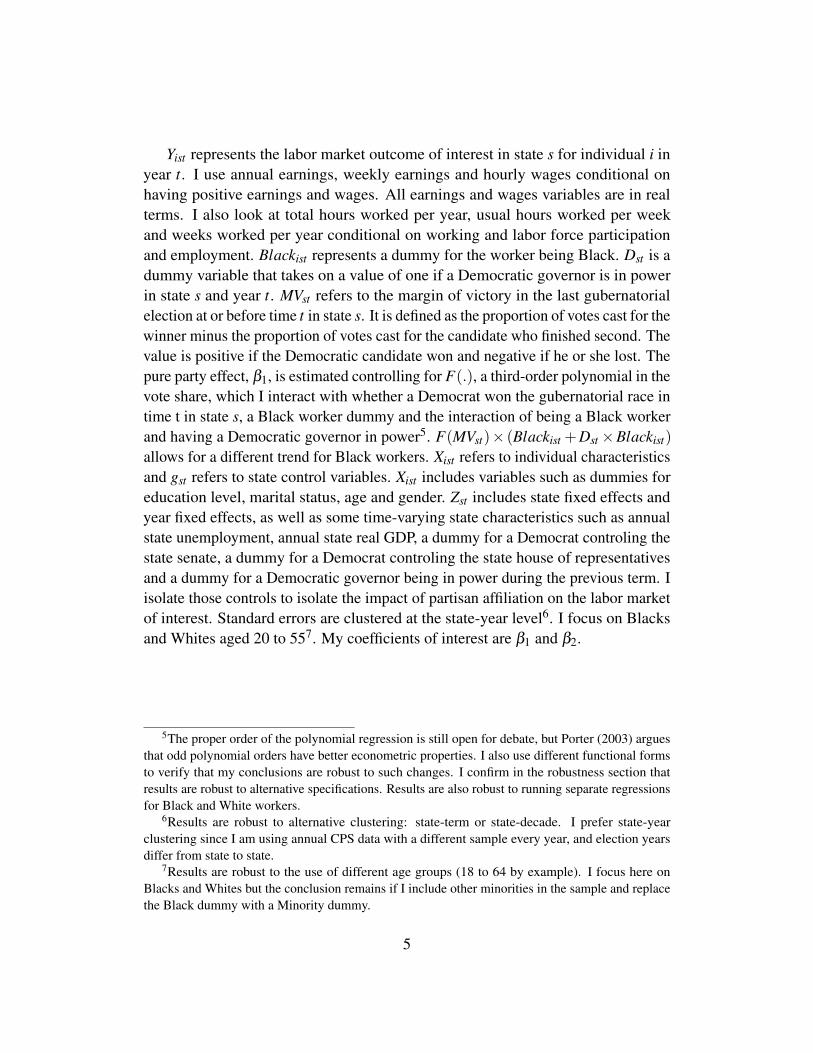
IV.C GRAPHICAL EVIDENCE

Figures A to D explore the discontinuity at 0% when a Democratic governor barelywins over a Republican for aggregate data. Figure A presents log annual earningsand Figure B presents the log annual earnings gap between Whites and Blacks. TheWhite and Black earnings gap is calculated by subtracting mean Black earningsfrom mean White earnings. Figure C presents the proportion of Whites and Blacksemployed. Figure D presents the hours worked by White and Black workers.

Each dot in the panels corresponds to the average outcome that follows election

10As mentioned above, I exclude in my sample cases when an independent governor won or whenthere is a death within a term and the party in power changes.

7

t, grouped by margin of victory intervals. The solid lines in the figures represent thepredicted values from the cubic polynomial fit without covariates. The horizontalaxis is the margin of victory in % and the vertical axis is the outcome of interest.Graphical evidence suggests that a decrease in average earnings for Whites and in theWhite and Black earnings gap occurs at the discontinuity. It also suggests that thereis a higher proportion of Blacks who work under Democratic governors and thatthey are working more hours. I estimate these effects precisely in the next section,using controls listed above to isolate the effect of partisan allegiance of governors onlabor market outcomes.

[FIGURES A to D]

V. MAIN RESULTS

Tables 2, 3, and 4 present results from the estimation of the baseline specification (1)for the variables Democratic governor, Democratic governor × Black, and Black,respectively. β1 and β2 are the coefficients of interest. β3 presents the pure effect ofbeing a Black worker on the labor market outcomes of interest. β2 and β3 togethershow the impact of a Democratic governor on Blacks. Column 1 presents results forall Black and White men and women, and columns 2 and 3 present results for menand women separately.

V.A EARNINGS (CONDITIONAL ON WORKING)

Table 2 presents results when the dependant variables are real annual earnings,real weekly earnings and real hourly wages11. The results indicate that under aDemocratic regime, annual earnings, weekly earnings and hourly earnings are lower

11Tables 1B, 2B and 3B in Appendix B present results for annual and weekly earnings and hourlywages. Each column adds additional controls. Column 1 present results with controls for state andyear fixed effects. Column 2 also controls for each states annual GDP and unemployment. Column3 adds controls for individual characteristics and column 4 adds the F(MVst)× (Dst +Blackist +

Dst ×Blackist) and Dst ×Blackist interactions. Column 5 adds controls for actions by other levelsof government, and a dummy for a Democratic governor being in power during the previous term.Column 5 is a replication of Table 2 in the text. Column 6 adds more time-varying state characteristicssuch as population, proportion of the population that is Black, proportion of the population that hasgraduated college, proportion of the population that has a graduate degree, and the proportion of thepopulation that has not attended high school. The impact of Democratic governors is robust acrossspecifications for all three measures of earnings.

8

on average, and that this decrease is larger for men than for women. Coefficientsfor men, which are −2.22% for annual earnings, −1.97% for weekly earnings and−1.49% for hourly wages, are statistically significant at the 1% level for all measuresof earnings and wages. Coefficients for females are −1.43% for annual earnings,−1.77% for weekly earnings, and −1.46% for hourly wages. Weekly earnings andhourly wages are significant at the 5% level for women, but annual earnings are not.

[TABLE 2]

Table 2 also provides evidence that partisan affiliation plays a role in the Blackand White earnings gap. Democratic governors have a positive impact on Blacksearnings relative to Whites earnings. The impact is 5.77% for men and 5.03% formen and women combined. These effects are both statistically significant. Thecoefficient for women is positive, but not statistically significant at the 5% level.The Black × Democratic governor interactions which represent the impact ofDemocratic governors on Black workers are positive but not significant for weeklyearnings and hourly wages. There is a decrease in the annual earnings gap betweenBlacks and Whites, but not in weekly earnings and hourly wages. This suggests thereis an increase in hours worked and employment of Black workers under Democraticgovernors. This is indeed confirmed in Table 3 and 4.

V.B TOTAL HOURS, WEEKS AND USUAL HOURS WORKED

Table 3 presents results for the following dependent variables: total hours worked peryear, weeks worked per year and usual hours per week. This section evaluates howmuch more or less an individual works when a Democrat is in power, conditional onthat individual working. Democratic governors do not have a significant impact onthe intensive margins for Whites (except for usual hours worked). However, Blacksincrease their hours worked more relative to Whites under a Democratic regimethan a Republican one. On average, Black men increase their hours worked peryear (4.66%) relative to White men under Democratic governors. They also increasetheir weeks worked (2.80%) and hours worked per week (1.85%). All results arestatistically significant at the 5% level. Results for Black women are less pronounced.Only their weeks worked per year are statistically significantly increased relative toWhites under a Democratic governor (2.88%).

[TABLE 3 AND TABLE 4]

9

V.C LABOR MARKET PARTICIPATION (IN LABOR FORCE AND EMPLOY-MENT)

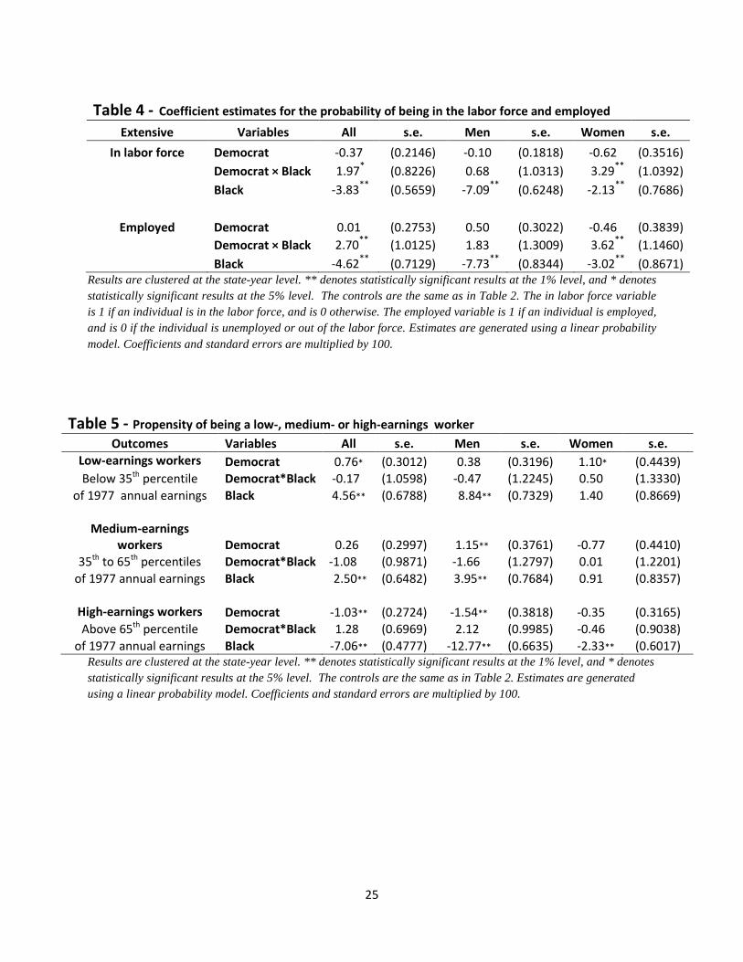
Table 4 shows results when the dependant variables measure labor force participationand employment. Coefficients for β1, β2 and β3 of specification (1) are estimatedusing a linear probability model12. Table 4 shows that the political party of the gover-nor has an impact on Black labor force participation and employment, especially forBlack women. The impact of Democratic governors on labor force participation andbeing employed for Black women are 3.29% and 3.62% respectively (and significantat 1%). The respective coefficient for men is positive but not significant.

VI. VALIDITY, ROBUSTNESS CHECKS AND

EXPLORATIONS

VI.A MODEL SPECIFICATION

I perform a number of robustness checks to ensure that my results are robust. Ibegin by investigating the underlying key assumption of the RDD approach, whichis that states where a Democratic governor barely wins are similar to states where aRepublican barely wins. I verify and confirm that states close to the discontinuity aresimilar along a number of dimensions. As in Ferreira and Gyourko (2009), I estimateregression discontinuity specifications using variables for state characteristics asdependent variables. I use aggregate data and an aggregate version of specification(1) without the individual characteristics. I find that the coefficient associated witha Democratic governor is never significant for these outcome variables, whichindicates that states are not statistically significantly different near the discontinuity.The RDD coefficients (with standard errors in brackets) for a Democratic governorare: proportion of the population that is Black [0.1352 (0.1229)], proportion of thepopulation for whom the highest level of study is elementary education [-0.16325(0.2196)], proportion of the population for whom the highest level of study is somehigh school or a high school diploma [0.2633 (0.2087)] , proportion of the populationfor whom the highest level of study is some college [-0.0675 (0.1305)], proportion ofthe population with a college degree or more studies [-0.0325 (0.2082)], proportionof the population aged less than 20 [0.1658 (0.1789)], proportion of the population

12With interactions terms, the linear probability model specification has better statistical propertiesthan a probit. Results are similar using the marginal effect of the probit.

10

aged more than 55 [-0.1839 (0.1886)], and proportion of the population aged 20to 55 [0.0075 (0.1783)]. Coefficients and standard errors are multiplied by 100.Descriptive statistics are also presented in Table 1.

Results are also robust to alternative polynomial forms. As mentioned above, theoptimal polynomial order is still up for debate. Results and conclusions are robustto a 1st-, 2nd- or 4th-order polynomial. Results are also robust to running separateregressions for Black and White workers. Another test performed is to limit themaximal margin of victory and drop elections that are far from the discontinuity.Results, significance and conclusions remain if I only keep elections where themargin of victory is less than 40%.

VI.B POSSIBLE HETEROGENEITY OF PARTISAN ALLEGIANCE

To ensure results are stable, I also estimate baseline regressions (using the specifi-cation from Table 2) for different samples of years and states and find that whilethe coefficients (slightly) vary depending on years and states used, the main effects,significance and conclusions remain. One interesting subsample is non-southernstates. Democrats in the south are arguably more conservative and therefore moresimilar to Republicans (Alt and Lowry, 2000). Therefore, one might expect that theeffects of a Democratic governor relative to a Republican would be more markedin non-southern states. I find that for non-southern states, the negative effect ofDemocratic governors on earnings is stronger and the positive impact of Democraticgovernor on labour market outcomes for Black people is more pronounced13. Oneother interesting subsample for robustness is restricting the sample to states thatfrequently elect both Democrats and Republicans (as opposed to states that consis-tently elect a governor from a single party)14. Results and conclusions are robust tofocusing on these states only.

VI.C POSSIBLE CONFOUNDING VARIABLES AND FACTORS

Another test is to include more state- and time-varying characteristics to isolate theimpact of the gubernatorial election. Results are robust to the addition of controls for

13Southern states are defined using the Census classification: Alabama, Arkansas, Delaware,Florida, Georgia, Kentucky, Louisiana, Maryland, Mississippi, North Carolina, Oklahoma, SouthCarolina, Tennessee, Texas, Virginia, West Virginia.

14I keep in this subsample states where Democrats and Republicans were each in power at least30% of the time over the years.

11

population, proportion of the population that is Black, proportion of the populationthat graduated college, proportion of the population with a graduate degree, andproportion of the population that did not attend high school. Results are also robustto the inclusion of dummies for the governor being a woman or from a minorityethnic group. They are also robust to controlling for state voter ideology using scoresfrom Carroll et al. for the state’s legislators in a given year15. Results are also robustto the inclusion of region × time dummies for the following regions (as definedin the CPS): Northeast, Midwest, South and West. Results are also robust to theexclusion of the first year a governor is in power, to remove potential lags in policy.To further investigate if my results are not due to long-term trends, I include a controlfor average earnings during the last term. Results and conclusions remain16. Resultsand interpretation are similar if the sample is restricted to full-time employees or if Iinclude major occupation and industry dummies.

Overall, results are very robust to alternative specifications and a rich set oftime-varying state characteristics.

VII. WORKFORCE CHANGES, CHANNELS AND

POLICIES

This paper has established that, on average, Democratic governors have differingeffects on the labor market than Republicans. When Democratic governors are inpower, the following three effects take place: i) a decrease in average earnings, ii) adecrease in the earnings gap between White and Black workers, and iii) an increasein Blacks employment.

In this section, I examine the mechanisms through which governors exercise theirinfluence over the labor market. I provide evidence that under Democratic governors,there is an increase of low- and medium-earnings workers and that this change inworkforce composition is a main factor explaining the decrease in earnings. I thenreview potential policies through which the increase in low- and medium- earningsworkers and the increase in Blacks employment happens.

15Scores from Carroll et al. are downloaded from http://voteview.com/dwnomin.htm (updatedFebruary 2011). I drop all legislators except Democrats and Republicans, and use the 1st dimensioncoordinate, which they describe as measuring liberalism or conservatism.

16I have missing values in some states in earlier years, since state variables in CPS data are availablestarting in 1977. (I reran the specification from Table 2 on this sample without a variable for averageearnings in the last term, and the results and conclusions remained.)

12

VII.A IMPACT ON LABOR FORCE COMPOSITION

To study the impact of partisan allegiance on workforce composition, I first divideworkers into three categories: low earnings, medium earnings and high earningswrokers. Low-earnings workers are defined as those whose earnings are below the35th percentile, measured in 1977 real earnings (at the national level). Medium-earnings workers are between 35th and 65th percentiles, and high-earnings workersare those above the 65th percentile17. Each worker in the sample is divided inthose three categories. I use this approximation to study the impact of Democraticgovernors on the workforce composition relative to Republicans. It is a simple butefficient way to cut the data to see if partisan affiliation alters labor force composition.The objective is to investigate whether political parties affect the probability ofbeing a low-, medium- or high-earnings worker. I do the exercise based on annualearnings18.

[TABLE 5]

Table 5 shows that the probability of being a low-earnings worker increases (and,for men only, the probability of being a medium- earnings worker increases) whenDemocratic governors are in power, while the probability of being a high- earningsworker decreases. However, one cannot determine from Table 5 if this effect iscaused by an entry of low-earnings workers, high-earnings workers transitioning tolower earnings, or a combination of these two factors.

I use the log of the number of workers in each of the three earnings categories asdependant variables and a modified version of specification (1) to investigate whichexplanation is most likely19. The results are provided in Table 6, which suggeststhat the effect is caused by an increase in the number of low- earnings workers.Moreover, policies in the literature and studied below suggest labor force entry bylow- and medium- earnings workers.

[TABLE 6]

Another way to study the labor force participation and employment probability is tolook at propensity to work by education categories. In Table 7, I study the probability

17Results are robust to alternative definitions of low- earnings, medium- earnings and high-earnings.

18Results are similar for hourly wage.19I use an aggregate version of specification (1) without the F(MVst)× (Dst +Blackist +Dst ×

Blackist) and Dst ×Blackist interactions, since the entry of low- earnings workers into the labormarket is the likely channel through which the effect on Black extensive margins occurs.

13

of employment and the probability of being in the labor force (dummy 0-1) of peoplewith high school diploma or less versus other levels of education using an interactionterm20. Table 7 shows that under Democratic governors, less educated worker workmore respective to more educated worker. Certainly, it is possible that less educatedworkers enter the labor market and earn a lot, but we know that it is unlikely thatnewcomer earn more than average. Table 7 also points to the same conclusion asabove.

[TABLE 7]

VII.B INCLUDING THE SHARE OF LOW- AND MEDIUM- EARNINGS WORK-ERS IN THE EARNINGS REGRESSION

The above section shows that under Democratic governors, there are changes inworkforce composition and there are more low- and medium- earnings workers. Animportant next step is to determine whether this change is driving the decrease inearnings under democratic governors.

To investigate if the changes in the labor force composition are a main fac-tor explaining the results, I do a simple test. I include variables for the share oflow-earnings workers and medium-earnings workers as additional controls. I runregressions for annual earnings, weekly earnings and hourly wages using a modifi-cation of specification (1)21. Results presented in Table 8 shows that the impact ofDemocratic governors on earnings almost disappears, completely when controllingfor labor force composition, such that results are no longer statistically significant.Thus, a change in labor force composition is a key factor explaining the aboveresults.

[TABLE 8]

VII.C POLICIES AND CHANNELS

Overall, the evidence points to the partisan allegiance of governors having an impacton the composition of the labor force by increasing low- and medium- earnings

20I use specification (1) without the F(MVst)× (Dst +Blackist +Dst ×Blackist) and Dst ×Blackist

interactions. I put an interaction between having a high school diploma or less education and aDemocrat being the governor.

21I once again use specification (1) without the F(MVst)× (Dst +Blackist +Dst ×Blackist) andDst ×Blackist interactions.

14

workers. This in turn results in a decrease in average earnings. The results also showan increase in the employment of Blacks. In this section, I examine what policiesmay lead to these results.

The above findings are likely the result of a combination of policies. In particular,I find that Democratic governors tend to be associated with higher public-sectoremployment, increased job protection as defined using the Displaced worker survey,(slightly) higher minimum wages, lower incarceration rates, and higher state earnedincome tax credit (EITC) rates, and that these policies contribute to the increasein the number of low- and medium-earnings workers and/or the increase in theBlacks intensive margins. However, I do not find that taxation (both corporate andpersonal) and business sector dynamics (firm entry rate, firm exit rate, firm jobcreation rate, firm job destruction rate, firm net job creation rate) to be affected bypartisan allegiance and therefore do not play a role in explaining the above results.Table 9 presents policies considered and summarized which policy is affected bypartisan allegiance of the governor. Detailed estimates are contained in AppendicesC through G.

[TABLE 9]

I find that Democratic governors have a small but statistically significant impacton the probability that a woman works in the public sector (0.42%) and the proba-bility that any worker works in the public sector (0.23%). These jobs tend to be inthe low- and medium- earnings categories. In other words, Democratic governorsincrease the proportion of low- and medium- earnings workers by increasing em-ployment in the public sector.

Democratic governors are also found to affect worker displacement. Using theDisplaced Worker Survey (January CPS) to investigate whether Democratic gover-nors affect the probability of being displaced, I find that Black men are less likelyto be a displaced worker under Democratic Governors (−2.11% and statisticallysignificant at the 5% level)22. This suggests an increase in the intensive marginsof Black men. Moreover, under Democratic governors, displaced workers are lesslikely to be low-earnings workers and more likely to be high-earnings workers23.These findings contribute to the increase in the share of low- and medium-earnings

22The Displaced Worker Survey has the same control variables as March CPS and the data isavailable every two years from 1984 to 2008. The definition of displaced worker used here is similarto Neal (1995).

23Leigh (2008) calls this a policy and economic conditions variable, which represent intermediateoutcomes resulting from policy choices and economic conditions (i.e. a function of both the supplyof, and demand for, welfare).

15

workers in the labor market.The literature suggests that Democratic governors are associated with (slightly)

higher minimum wages (Besley and Case, 1995 and Leigh, 2008) and lower in-carceration rates (Leigh, 2008). Both measures could increase the labor supply oflow-earnings workers. I find that, by adding state minimum wages to specification(1), minimum wage has a positive and significant impact on total hours worked forlow-earnings workers, and has a significant positive impact on labor force partici-pation and employment for low-earnings workers. Doing the same exercise withstate incarceration rates, I find that a higher incarceration rate has a significant nega-tive impact on labor force participation and employment for low-earnings workers.Neither the minimum wage nor the incarceration rates affect overall employment.My results for the minimum wage are in accordance with studies such as Card andKrueger (1994, 2000). Moreover, a higher proportion of Black workers than Whiteworkers earn minimum wage, which helps explain the decrease in the earnings gapbetween Blacks and Whites.

State earned income tax credits (EITC) can also help explain my results. EITCis a refundable tax credit primarily for individuals and couples with children. Theindirect effect of the policy is to increase employment, mostly of low- and medium-earnings workers, particularly women. I find that Democratic governors increasethe probability that a state offers an EITC and are also associated with higher levelsof EITC24. Adding state EITC rates to specification (1) shows that state EITC rateshave a positive significant impact on total hours worked, labor force participationand employment for low-earnings women. Moreover, state EITC rates do not reduceoverall employment.

I also investigate other channels, such as taxation (both corporate and personal)and business dynamics, which could affect workforce composition. I examinewhether the decrease in earnings found in previous tables remains after including in-come taxes using the NBER Taxsim simulator. As in Reed (2006) and Leigh (2008),I do not find that the partisan affiliation of governors has an impact on personaltaxation or on the progressivity of the tax system. Taxation is not a factor explainingthe increase of low- and medium-earnings workers25. To study business dynamics, Iuse the following outcome variables provided by the U.S. Census Bureaus Business

24I focus on 1990 to 2008, when several states implemented an EITC. Data aboutstate EITC are taken from UKCPR. More details about state EITC are available athttp://www.irs.gov/individuals/article/0,,id=177866,00.html.

25I use family earnings because of the joint filing for married couples in the U.S. tax system.After-tax income is obtained using the NBER TAXSIM simulator and before-tax income and certaintax credits are obtained from the CPS. I use code provided by James P. Ziliak to incorporate tax creditsvariables from the CPS into the NBER TAXSIM simulator. The CPS does not have information on

16

Dynamics Statistics: establishment entry rate, establishment exit rate, firms jobcreation rate, firms job destruction rate, and firms net job creation rate26. I do notfind that business dynamics are affected by gubernatorial political allegiance. Usingthe top corporate tax rate as an outcome variable, I do not find that the partisanallegiance of the governor has an impact on corporate taxation.

VIII. CONCLUSION

This paper is a comprehensive study of the causal impact of partisan allegiance ofU.S. governors on labor market outcomes using a regression discontinuity approachto remove potential endogeneity of election results. Results indicate that the partisanallegiance of U.S. governors affects earnings and that Democratic governors areassociated with lower individual earnings. Moreover, results presented in thispaper provide evidence that Democratic governors reduce the average earnings gapbetween Black and White workers. Blacks also increase their labor supply morerelative to Whites under Democratic governors. I provide evidence that there is anincrease of low- and medium-earnings workers under Democratic governors and thatthis change in the workforce composition is the main factor explaining the results.Results are robust to alternative specifications and a rich set of time-varying statecharacteristics. Although this paper improves the understanding of the importance ofpartisan allegiance at the state level, more work is needed in this area to understandthe full extent of the role of political parties. I have provided evidence of a short-term increase of low- and medium-earnings workers under Democratic governors.Subsequent research should investigate if this increase in participation has long-termbenefits for these groups, and whether there are effects on variables such as returnsto education and union wage premiums.

certain inputs for the TAXSIM program, such as annual rental payments, child care expenses, andother itemized deductions. These values are set to zero when calculating tax liability. The othervariables of the TAXSIM simulator are found in the CPS. Results of Table 1F are similar if creditsfrom the CPS are not included in the TAXSIM simulation.

26All variables are available for all of my sample years.

17

VIII.REFERENCES

[1] James E. Alt and Robert C. Lowry. A dynamic model of state budget outcomesunder divided partisan government. The Journal of Politics, 62(4):pp. 1035–1069.

[2] Gary Becker. The Economics of Discrimination. Chicago University Press,1971.

[3] Timothy Besley and Anne Case. Does electoral accountability affect economicpolicy choices? evidence from gubernatorial term limits. The Quarterly Journalof Economics, 110(3):769–798, 1995.

[4] Timothy Besley and Anne Case. Political institutions and policy choices:Evidence from the united states. Journal of Economic Literature, 41(1):pp.7–73, 2003.

[5] David Bjerk. The differing nature of black-white wage inequality acrossoccupational sectors. The Journal of Human Resources, 42(2):pp. 398–434,2007.

[6] Dan A. Black. Discrimination in an equilibrium search model. Journal ofLabor Economics, 13(2):pp. 309–334, 1995.

[7] Bryan Caplan. Has leviathan been bound? a theory of imperfectly con-strained government with evidence from the states. Southern Economic Journal,67(4):pp. 825–847, 2001.

[8] David Card and Alan B. Krueger. Trends in relative black-white earningsrevisited. The American Economic Review, 83(2):pp. 85–91, 1993.

[9] David Card and Alan B. Krueger. Minimum wages and employment: A casestudy of the fast-food industry in new jersey and pennsylvania. The AmericanEconomic Review, 84(4):pp. 772–793, 1994.

[10] David Card and Alan B. Krueger. Minimum wages and employment: A casestudy of the fast-food industry in new jersey and pennsylvania: Reply. TheAmerican Economic Review, 90(5):pp. 1397–1420, 2000.

[11] Robert Jay Dilger. Does politics matter? partisanship’s impact on state spendingand taxes, 1985-95. State and Local Government Review, 30(2):pp. 139–144,1998.

18

[12] Robert S. Erikson, Jr. Wright, Gerald C., and John P. McIver. Political parties,public opinion, and state policy in the united states. The American PoliticalScience Review, 83(3):pp. 729–750, 1989.

[13] Fernando Ferreira and Joseph Gyourko. Do political parties matter? evidencefrom u.s. cities. The Quarterly Journal of Economics, 124(1):399–422, 2009.

[14] Fernando Ferreira and Joseph Gyourko. Does gender matter for politicalleadership? the case of u.s. mayors. Working Paper, 2011.

[15] James C. Garand. Explaining government growth in the u.s. states. TheAmerican Political Science Review, 82(3):pp. 837–849, 1988.

[16] John S. Heywood and Daniel Parent. Performance pay and the white-blackwage gap. Journal of Labor Economics, 30(2):249 – 290, 2012.

[17] Bridget Hunter. State governors play key role in u.s. government.

[18] Guido Imbens and Thomas Lemieux. Regression discontinuity designs: Aguide to practice. Journal of Econometrics, 142(2):615–635, 2008.

[19] Jeff Larrimore, Richard Burkhauser, Shuaizhang Feng, and Laura Zayatz.Consistent cell means for topcoded incomes in the public use march cps (1976-2007). Journal of Economic and Social Measurement, 33(2-3):pp. 89–128,2008.

[20] David S. Lee. The electoral advantage to incumbency and voters’ valuation ofpoliticians’ experience: A regression discontinuity analysis of elections to theu.s house. Working Paper 8441, National Bureau of Economic Research, 2001.

[21] David S. Lee. Randomized experiments from non-random selection in u.s.house elections. Journal of Econometrics, 142(2):675–697, 2008.

[22] David S. Lee and Thomas Lemieux. Regression discontinuity designs ineconomics. Journal of Economic Literature, 48(2):281–355, June 2010.

[23] David S. Lee, Enrico Moretti, and Matthew J. Butler. Do voters affect or electpolicies? evidence from the u. s. house. The Quarterly Journal of Economics,119(3):pp. 807–859, 2004.

[24] Andrew Leigh. Estimating the impact of gubernatorial partisanship on pol-icy settings and economic outcomes: A regression discontinuity approach.European Journal of Political Economy, 24(1):256–268, 2008.

19

[25] Justin McCrary. Manipulation of the running variable in the regression dis-continuity design: A density test. Journal of Econometrics, 142(2):698–714,February 2008.

[26] Derek Neal. Industry-specific human capital: Evidence from displaced workers.Journal of Labor Economics, 13(4):pp. 653–677, 1995.

[27] Derek A. Neal and William R. Johnson. The role of premarket factors in black-white wage differences. Journal of Political Economy, 104(5):pp. 869–895,1996.

[28] Per Pettersson-Lidbom. Do parties matter for economic outcomes? a regression-discontinuity approach. Journal of the European Economic Association,6(5):pp. 1037–1056, 2008.

[29] Robert D. Plotnick and Richard F. Winters. A politico-economic theory ofincome redistribution. The American Political Science Review, 79(2):pp. 458–473, 1985.

[30] Jack Porter. Estimation in the refression discontinuity model. Working Paper,University of Wisconsin, 2003.

[31] James M. Poterba. State responses to fiscal crises: The effects of budgetaryinstitutions and politics. Journal of Political Economy, 102(4):pp. 799–821,1994.

[32] W. Robert Reed. Democrats, republicans, and taxes: Evidence that politicalparties matter. Journal of Public Economics, 90(4-5):725–750, 2006.

[33] Finis Welch. Black-white differences in returns to schooling. The AmericanEconomic Review, 63(5):pp. 893–907, 1973.

[34] James P. Ziliak, Bradley Hardy, and Christopher Bollinger. Earnings volatilityin america: Evidence from matched cps. Labour Economics, 18(6):742–754,2011.

20

21

Figures

Figure A: Partisan identity and Annual Earnings (A)

Figure B: Partisan identity and the White and Black annual earnings gap

22

Figure C: Partisan identity and the proportion of Whites (left) and Blacks (right) who work

Figure D: Partisan identity and total hours worked per year for Whites (left) and Blacks (right)

23

Tables

Table 1 Table 1A - Descriptive statistics of selected variables for states close to discontinuity

Black Elementary

Some HS

& HS Some

College Margin of victory less 5 % Republican 10.03 28.24 37.71 11.75 Sd (0.6281) (0.2922) (0.3751) (0.2873) Democrat 9.95 27.79 37.71 11.76 Sd (0.8156) (0.3060) (0.3185) (0.3031) Margin of victory less 10 % Republican 9.92 28.49 38.14 11.65 Sd (0.5144) (0.2044) (0.2739) (0.2183) Democrat 9.59 28.13 38.01 11.74 Sd (0.5421) (0.2316) (0.2240) (0.2199)

Mean and standard deviation of the mean for the proportion of the population close to the discontinuity that is Black, and by highest level of education completed (elementary school, some high school or a high-school diploma, and some college). Coefficients and standard errors are multiplied by 100.

Table 1B - Descriptive statistics of selected variables for states close to discontinuity

College & Grad

School Age<20 Age>55 Age 20 to

55 Margin Victory ≤ 5 % Republican 22.30 30.82 21.22 50.51 sd (0.3643) (0.2369) (0.2046) (0.1596) Democrat 22.08 31.12 21.00 50.43 sd (0.2885) (0.2547) (0.2891) (0.1971) Margin Victory ≤ 10 % Republican 21.72 31.03 21.32 50.18 sd (0.2474) (0.1696) (0.1555) (0.1167) Democrat 22.12 31.21 21.00 50.37 sd (0.2195) (0.1835) (0.1898) (0.1415)

Mean and standard deviation of the mean for proportion of population close to the discontinuity with at least a college degree, of age 20 or less, aged more than 55, and aged 20 to 55. Coefficients and standard errors are multiplied by 100.

24

Table 2 - Coefficient estimates for annual and weekly earnings and hourly wages Earnings Variables All s.e. Men s.e. Women s.e. Annual Democrat -1.96** (0.6050) -2.22** (0.6916) -1.43 (0.8927)

Democrat × Black 5.03** (1.8880) 5.77* (2.3489) 2.80 (2.5085) Black -15.57** (1.2034) -29.18** (1.4591) -5.01** (1.6372)

Weekly Democrat -1.95** (0.5164) -1.97** (0.6219) -1.77** (0.6819) Democrat × Black 2.00 (1.4696) 2.97 (1.8236) -0.08 (1.9456) Black -9.82** (0.9325) -20.49** (1.1087) -1.32 (1.3089)

Hourly Democrat -1.53** (0.4629) -1.49** (0.5619) -1.46* (0.5917) Democrat × Black 1.00 (1.2693) 1.11 (1.6993) 0.10 (1.5777)

Black -9.35** (0.8290) -15.30** (1.0355) -4.58** (1.0573) Results are clustered at the state-year level. ** denotes statistically significant results at the 1% level, and * denotes statistically significant results at the 5% level. Controls variables include highest level of education, marital status, age, age2, age3, age4, a female dummy, state fixed effect, year fixed effect and time-varying characteristics such as annual state unemployment, annual state real GDP, a dummy for Democrat control of the state senate, a dummy for Democrat control of the state house and a dummy for a Democratic governor being in power during the previous term. Outcome variables are expressed in log and coefficients and standard errors are multiplied by 100.

Table 3 - Coefficient estimates for total hours worked, weeks worked and usual hours Intensive Variables All s.e. Men s.e. Women s.e.

Total hours worked Democrat -0.44 (0.4162) -0.74 (0.4293) 0.02 (0.6424)

Democrat × Black 4.03** (1.2579) 4.66** (1.6275) 2.70 (1.7703) Black -6.22** (0.8399) -13.87** (1.0494) -0.43 (1.1733)

Weeks worked Democrat -0.02 (0.3213) -0.26 (0.3352) 0.34 (0.4751) Democrat × Black 3.03** (0.9733) 2.80* (1.3114) 2.88* (1.3362) Black -5.75** (0.6643) -8.68** (0.8429) -3.69** (0.9311)

Usual hours Democrat -0.42* (0.2074) -0.48* (0.2227) -0.31 (0.3303) Democrat × Black 1.00 (0.5441) 1.85** (0.6615) -0.18 (0.9132)

Black -0.47 (0.3451) -5.19** (0.4589) 3.26** (0.6077) Results are clustered at the state-year level. ** denotes statistically significant results at the 1% level, and * denotes statistically significant results at the 5% level. The controls are the same as in Table 2. Outcome variables are expressed in log form and coefficients and standard errors are multiplied by 100.

25

Table 4 - Coefficient estimates for the probability of being in the labor force and employed Extensive Variables All s.e. Men s.e. Women s.e.

In labor force Democrat -0.37 (0.2146) -0.10 (0.1818) -0.62 (0.3516) Democrat × Black 1.97* (0.8226) 0.68 (1.0313) 3.29** (1.0392) Black -3.83** (0.5659) -7.09** (0.6248) -2.13** (0.7686)

Employed Democrat 0.01 (0.2753) 0.50 (0.3022) -0.46 (0.3839) Democrat × Black 2.70** (1.0125) 1.83 (1.3009) 3.62** (1.1460)

Black -4.62** (0.7129) -7.73** (0.8344) -3.02** (0.8671) Results are clustered at the state-year level. ** denotes statistically significant results at the 1% level, and * denotes statistically significant results at the 5% level. The controls are the same as in Table 2. The in labor force variable is 1 if an individual is in the labor force, and is 0 otherwise. The employed variable is 1 if an individual is employed, and is 0 if the individual is unemployed or out of the labor force. Estimates are generated using a linear probability model. Coefficients and standard errors are multiplied by 100.

Table 5 - Propensity of being a low-, medium- or high-earnings worker Outcomes Variables All s.e. Men s.e. Women s.e.

Low-earnings workers Democrat 0.76* (0.3012) 0.38 (0.3196) 1.10* (0.4439) Below 35th percentile Democrat*Black -0.17 (1.0598) -0.47 (1.2245) 0.50 (1.3330)

of 1977 annual earnings Black 4.56** (0.6788) 8.84** (0.7329) 1.40 (0.8669)

Medium-earnings workers Democrat 0.26 (0.2997) 1.15** (0.3761) -0.77 (0.4410)

35th to 65th percentiles Democrat*Black -1.08 (0.9871) -1.66 (1.2797) 0.01 (1.2201) of 1977 annual earnings Black 2.50** (0.6482) 3.95** (0.7684) 0.91 (0.8357)

High-earnings workers Democrat -1.03** (0.2724) -1.54** (0.3818) -0.35 (0.3165) Above 65th percentile Democrat*Black 1.28 (0.6969) 2.12 (0.9985) -0.46 (0.9038)

of 1977 annual earnings Black -7.06** (0.4777) -12.77** (0.6635) -2.33** (0.6017) Results are clustered at the state-year level. ** denotes statistically significant results at the 1% level, and * denotes statistically significant results at the 5% level. The controls are the same as in Table 2. Estimates are generated using a linear probability model. Coefficients and standard errors are multiplied by 100.

26

Table 6 – Coefficient estimates for number of workers in each category

Number of low-earnings workers Below 35th percentile Democrat 2.13* (1.0464)

of 1977 annual earnings

Number of medium-earnings workers 35th to 65th percentiles Democrat 0.64 (1.1153) of 1977 annual earnings

Number of high-earnings workers

Above 65th percentile Democrat -0.46 (1.1412) of 1977 annual earnings

Results are clustered at the state-year level. ** denotes statistically significant results at the 1% level, and * denotes statistically significant results at the 5% level. Estimates are generated using an aggregate version of specification (1) without the F(MVst ) × (Blackist + Dst × Blackist ) and Dst × Blackist interactions. Coefficients and standard errors are multiplied by 100.

Results are clustered at the state-year level. ** denotes statistically significant results at the 1% level, and * denotes statistically significant results at the 5% level. Estimates are generated using a regression of equation (1) without the F(MVst ) × (Dst + Blackist + Dst × Blackist ) and Dst× Blackist interactions for annual and weekly earnings and hourly wages and controls for the share of low- and medium-earnings workers. Additional controls are the same as in Table 2. Outcome variables are expressed in log form and coefficients and standard errors are multiplied by 100.

Table 7 - Regression for probability of being in labor force and employed Table 7 - Regression for probability of being in labor force and employed Table 7 - Regression for probability of being in labor force and employed

Extensive Variables All Std Men Std Women Std In Labor Democrat -0.51* (0.2337) -0.37 (0.2649) -0.76* (0.3313)

force Democrat*(<=high school diploma) 0.73** (0.2367) 1.13** (0.2428) 0.61 (0.3117)

Employed Democrat -0.72** (0.2796) -0.46 (0.3255) -1.10** (0.3851)

Democrat*(<=high school diploma) 0.66* (0.2752) 1.10** (0.2953) 0.51 (0.3271)

27

Table 8 - Coefficient estimates for annual, weekly and hourly earnings including share of workers. Earnings Variable All s.e. Men s.e. Women s.e. Annual Democrat -0.39 (0.5326) -0.61 (0.6446) -0.18 (0.8147) Weekly Democrat -0.74 (0.4094) -0.60 (0.5307) -0.94 (0.5808) Hourly Democrat -0.53 (0.3660) -0.38 (0.4711) -0.72 (0.5154) Includes the share of yes yes yes low- and medium-earnings workers

Results are clustered at the state-year level. ** denotes statistically significant results at the 1% level, and * denotes statistically significant results at the 5% level. Estimates are generated using a regression of equation (1) without the F(MVst ) × (Dst + Blackist + Dst × Blackist ) and Dst× Blackist interactions for annual and weekly earnings and hourly wages and controls for the share of low- and medium-earnings workers. Additional controls are the same as in Table 2. Outcome variables are expressed in log form and coefficients and standard errors are multiplied by 100.

Table 9 - Summary Tables of policiesPolicy Partisan Allegiance has significan impact? Impact of DemocratsState Public Sector Yes Increse employment

in public sectorBusiness Sector No(via Business Dynamics Statistics) -

Job Protection Yes Black are less displaced(via Displaced Worker Survey) Displaced worker are less low earners

Taxation Corporate No - Household -

Minimun Wage Yes Sligthly higher

Incarceration Rate Yes Lower

State EITC Yes More frequent and higher

Appendix - Political Parties & Labor Market Outcomes Appendix A - Descriptive Statistics

Table A1 - Frequency in power All Years - 1977 to 2008 Frequency % Republican Governors 730 46.62% Democratic Governors 836 53.38% 1977 to 1993 Frequency % Republican Governors 317 38.06% Democratic Governors 516 61.94% 1994 to 2008 Frequency % Republican Governors 413 56.34% Democratic Governors 320 43.66%

Frequency each political party is in power in the sample.

Table A2 - Mean values of key variables Categories Variables Mean Sd Outcomes ln(Annual Earnings) 9.8758 (1.1133) ln(Weekly Earnings) 6.1178 (0.8746) ln(Hourly Earnings) 2.4817 (0.7556) ln(Weeks worked) 3.7580 (0.4976) ln(Usual hours) 3.6361 (0.3650) ln(Total hours) 7.3941 (0.7004)

Other Elections State house democrat 0.7108 (0.4534) State senate democrat 0.5911 (0.4916)

Macro ln(Real GDP) 12.3875 (0.9499) ln(unemployment rate) 1.7479 (0.2919)

Characteristics Black 0.1197 (0.3246) Female 0.4694 (0.4991) Age 36.1501 (9.9853) Education Elementary 0.0366 (0.1879)

High School 0.3405 (0.4739) Some college 0.1767 (0.3814) College 0.2818 (0.4499) More than college 0.0824 (0.2749)

Marital status Married 0.5954 (0.4908) Separated 0.0276 (0.1639) Divorced 0.1012 (0.3016) Widowed 0.0100 (0.0996) Never married 0.2658 (0.4418)

Appendix B- Earnings & Wages, adding more controls each column

Results are clustered at the state-year level. ** denotes statistically significant results at the 1% level, and * denotes statistically significant results at the 5% level. The controls are the same as in Table 2. The outcome variable (annual earnings) is measured in log form. Column 1 presents results with fixed effects for state and year. Column 2 adds controls for annual GDP per state and unemployment. Column 3 controls for individual characteristics and column 4 includes the F(MVst ) × (Dst + Blackist + Dst × Blackist ) and Dst× Blackist interactions. Column 5 adds other government level controls and a dummy for a Democrat being in power last term. Column 6 adds more time-varying state characteristics such as population, proportion of the population that is Black, the proportion of the population that is a college graduate, the proportion of the population with a graduate degree, and the proportion of the population that has completed elementary school.

Table B1 - Annual Earnings by stepVariables 1 s.e. 2 s.e. 3 s.e. 4 s.e. 5 s.e. 6 s.e.

All Democrat -2.63** (0.8964) -2.04** (0.7221) -1.25* (0.5908) -1.89** (0.6139) -1.96** (0.605) -2.09** (0.6253)Democrat × Black - - - - - - 5.1** (1.8873) 5.03** (1.888) 4.95** (1.8915)Black - - - - -12.02** (0.3798) -15.58** (1.202) -15.57** (1.2034) -15.57** (1.2088)

Male Democrat -3.13** (1.0897) -2.41** (0.8632) -1.61* (0.7093) -2.27** (0.6955) -2.22** (0.6916) -2.43** (0.6767)Democrat × Black - - - - - - 5.83* (2.3506) 5.77* (2.3489) 5.68* (2.345)Black - - - - -25.44** (0.4608) -29.16** (1.4562) -29.18** (1.4591) -29.23** (1.4649)

Female Democrat -2.39* (1.0317) -2.02* (0.9743) -0.78 (0.8378) -1.20 (0.8992) -1.43 (0.8927) -1.36 (0.9188)Democrat × Black - - - - - - 2.89 (2.5097) 2.8 (2.5085) 2.76 (2.5096)Black - - - - -2.86** (0.4965) -5.05** (1.6384) -5.01** (1.6372) -4.93** (1.6414)

Fixed effect yes yes yes yes yes yes(state & year)

GDP - yes yes yes yes yesUnemployment

Individual Character. - - yes yes yes yes

Black Interactions - - - yes yes yes

Other Governments - - - - yes yes

More state controls - - - - - yes

Results are clustered at the state-year level. ** denotes statistically significant results at the 1% level, and * denotes statistically significant results at the 5% level. The controls are the same as in Table 2. The outcome variable (weekly earnings) is measured in log form. Column 1 presents results with fixed effects for state and year. Column 2 adds controls for annual GDP per state and unemployment. Column 3 controls for individual characteristics and column 4 includes the F(MVst ) × (Dst + Blackist + Dst × Blackist ) and Dst× Blackist interactions. Column 5 adds controls for other levels of government and a dummy for a Democrat being in power last term. Column 6 adds more time-varying state characteristics such as population, the proportion of the population that is Black, the proportion of the population that is a college graduate, the proportion of the population with a graduate degree, and the proportion of the population that completed elementary school.

Table B2 - Weekly Earnings by stepVariables 1 s.e. 2 s.e. 3 s.e. 4 s.e. 5 s.e. 6 s.e.

All Democrat -2.63** (0.7343) -2.17** (0.6452) -1.55** (0.4959) -1.83** (0.523) -1.95** (0.5164) -1.67** (0.5128)Democrat × Black - - - - - - 2.08 (1.4694) 2.00 (1.4696) 1.94 (1.4701)Black - - - - -8.25** (0.2953) -9.83** (0.9309) -9.82** (0.9325) -9.84** (0.9369)

Male Democrat -2.69** (0.8794) -2.17** (0.7846) -1.58** (0.6155) -1.94** (0.6185) -1.97** (0.6219) -1.81** (0.5819)Democrat × Black - - - - - - 3.03 (1.8253) 2.97 (1.8236) 2.89 (1.8178)Black - - - - -18.97** (0.3513) -20.49** (1.107) -20.49** (1.1087) -20.55** (1.1132)

Female Democrat -2.84** (0.8119) -2.52** (0.7672) -1.51* (0.6254) -1.54* (0.6913) -1.77** (0.6819) -1.27 (0.6995)Democrat × Black - - - - - - 0.03 (1.9448) -0.08 (1.9456) -0.10 (1.9436)Black - - - - -0.72 (0.3797) -1.36 (1.308) -1.32 (1.3089) -1.3 (1.3096)

Fixed effect yes yes yes yes yes yes(state & year)

GDP - yes yes yes yes yesUnemployment

Individual Character. - - yes yes yes yes

Black Interactions - - - yes yes yes

Other Governments - - - - yes yes

More state controls - - - - - yes

Results are clustered at the state-year level. ** denotes statistically significant results at the 1% level, and * denotes statistically significant results at the 5% level. The controls are the same as in Table 2. The outcome variable (annual wage) is measured in log form. Column 1 presents results with fixed effects for state and year. Column 2 adds controls for annual GDP per state and unemployment. Column 3 controls for individual characteristics and column 4 includes the F(MVst ) × (Dst + Blackist + Dst × Blackist ) and Dst× Blackist interactions. Column 5 adds controls for other levels of government and a dummy for a Democrat being in power last term. Column 6 adds more time-varying state characteristics such as population, the proportion of the population that is Black, the proportion of the population that is a college graduate, the proportion of population with a graduate degree, and the proportion of the population that completed elementary school.

Table B3- Hourly Wages by stepVariables 1 s.e. 2 s.e. 3 s.e. 4 s.e. 5 s.e. 6 s.e.

All Democrat -2.19** (0.6305) -1.83** (0.5888) -1.27** (0.4447) -1.41** (0.4679) -1.53** (0.4629) -1.34** (0.4619)Democrat × Black - - - - - - 1.07 (1.270) 1.00 (1.2693) 0.94 (1.2684)Black - - - - -8.27** (0.2495) -9.36** (0.8278) -9.35** (0.829) -9.35** (0.8324)

Male Democrat -2.13** (0.7502) -1.72* (0.7064) -1.27* (0.549) -1.42* (0.5583) -1.49** (0.5619) -1.40** (0.5326)Democrat × Black - - - - - - 1.18 (1.6997) 1.11 (1.6993) 1.04 (1.696)Black - - - - -14.63** (0.3218) -15.3** (1.0344) -15.3** (1.0355) -15.34** (1.038)

Female Democrat -2.39** (0.6886) -2.12** (0.6684) -1.25* (0.5477) -1.28* (0.5965) -1.46* (0.5917) -1.12 (0.607)Democrat × Black - - - - - - 0.19 (1.5781) 0.10 (1.5777) 0.08 (1.5751)Black - - - - -3.85** (0.3059) -4.61** (1.0563) -4.58** (1.0573) -4.53** (1.0601)

Fixed effect yes yes yes yes yes yes(state & year)

GDP - yes yes yes yes yesUnemployment

Individual Character. - - yes yes yes yes

Black Interactions - - - yes yes yes

Other Governments - - - - yes yes

More state controls - - - - - yes

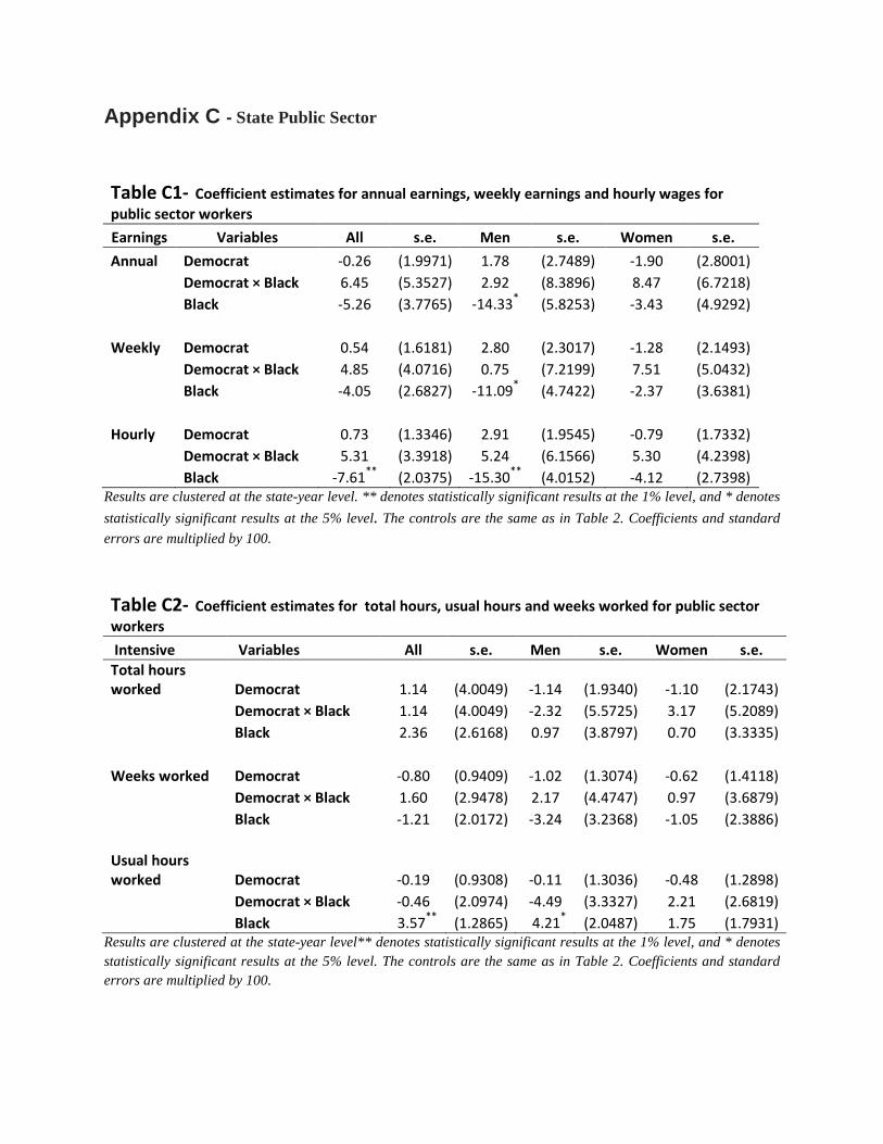
Appendix C - State Public Sector

Table C1- Coefficient estimates for annual earnings, weekly earnings and hourly wages for public sector workers Earnings Variables All s.e. Men s.e. Women s.e. Annual Democrat -0.26 (1.9971) 1.78 (2.7489) -1.90 (2.8001) Democrat × Black 6.45 (5.3527) 2.92 (8.3896) 8.47 (6.7218) Black -5.26 (3.7765) -14.33* (5.8253) -3.43 (4.9292) Weekly Democrat 0.54 (1.6181) 2.80 (2.3017) -1.28 (2.1493) Democrat × Black 4.85 (4.0716) 0.75 (7.2199) 7.51 (5.0432) Black -4.05 (2.6827) -11.09* (4.7422) -2.37 (3.6381) Hourly Democrat 0.73 (1.3346) 2.91 (1.9545) -0.79 (1.7332)

Democrat × Black 5.31 (3.3918) 5.24 (6.1566) 5.30 (4.2398) Black -7.61** (2.0375) -15.30** (4.0152) -4.12 (2.7398)

Results are clustered at the state-year level. ** denotes statistically significant results at the 1% level, and * denotes

statistically significant results at the 5% level. The controls are the same as in Table 2. Coefficients and standard

errors are multiplied by 100.

Table C2- Coefficient estimates for total hours, usual hours and weeks worked for public sector workers Intensive Variables All s.e. Men s.e. Women s.e. Total hours worked Democrat 1.14 (4.0049) -1.14 (1.9340) -1.10 (2.1743) Democrat × Black 1.14 (4.0049) -2.32 (5.5725) 3.17 (5.2089) Black 2.36 (2.6168) 0.97 (3.8797) 0.70 (3.3335) Weeks worked Democrat -0.80 (0.9409) -1.02 (1.3074) -0.62 (1.4118) Democrat × Black 1.60 (2.9478) 2.17 (4.4747) 0.97 (3.6879) Black -1.21 (2.0172) -3.24 (3.2368) -1.05 (2.3886) Usual hours worked Democrat -0.19 (0.9308) -0.11 (1.3036) -0.48 (1.2898)

Democrat × Black -0.46 (2.0974) -4.49 (3.3327) 2.21 (2.6819) Black 3.57** (1.2865) 4.21* (2.0487) 1.75 (1.7931)

Results are clustered at the state-year level** denotes statistically significant results at the 1% level, and * denotes statistically significant results at the 5% level. The controls are the same as in Table 2. Coefficients and standard errors are multiplied by 100.

Table C3- Coefficient estimates for the probability of working in the public sector Extensive Variables All s.e. Men s.e. Women s.e. State Public Democrat 0.23* (0.0988) 0.03 (0.1174) 0.42** (0.1420) sector Democrat × Black -0.15 (0.2951) -0.08 (0.3905) -0.21 (0.4283)

Black 1.25** (0.1801) 0.65** (0.2494) 1.73** (0.2480) Results are clustered at the state-year level. ** denotes statistically significant results at the 1% level, and * denotes statistically significant results at the 5% level. The controls are the same as in Table 2. Estimates are generated using a linear probability model for working in the state public sector. Coefficients and standard errors are multiplied by 100.

Appendix D – Business Sector

Table D1 - Impact of businesses Outcomes Variable All s.e. Establishment entry rate Democrat -20.32 (19.0981) Establishment exit rate Democrat -8.35 (14.4308) Job creation rate Democrat -14.91 (25.7231) Job destruction rate Democrat -26.60 (32.9170) Net job creation rate Democrat -38.70 (56.3691) Top corporate tax rate Democrat -2.94 (1.5786)

Results are clustered at the state-year level. ** denotes statistically significant results at the 1% level, and * denotes statistically significant results at the 5% level. Estimates are generated from Business Dynamics Statistics, using a regression of the aggregate version of specification (1) for the outcomes variables: establishment entry rate, establishment exit rate, job creation rate, job destruction rate and net job creation. Coefficients and standard errors are multiplied by 100.

Table D2 - Impact of businesses by firm size

Firm Size 0-100 100-500 500-1000

1000-2500

2500 & more

Outcomes Variables All All All All All Establishment entry rate Democrat -17.62 -14.94 -17.65 -17.47 -24.56 s.e. (14.9685) (23.3827) (38.4313) (42.2958) (16.7670) Establishment exit rate Democrat -2.63 9.11 15.76 -6.99 4.67 s.e. (10.8389) (17.1895) (31.9755) (40.4646) (13.4679) Job creation rate Democrat 1.74 -18.05 -97.49 -79.46 -43.94 s.e. (24.5423) (34.0811) (61.4491) (71.8663) (43.7873) Job destruction rate Democrat -4.83 -12.51 -84.46 -72.94 -95.10 s.e. (23.6890) (33.2656) (58.2737) (79.6551) (58.4003) Net job creation rate Democrat 6.57 -5.53 -13.02 -6.52 51.16 S.e. (33.6475) (46.1136) (75.5415) (107.9566) (73.8913)

Results are clustered at the state-year level. ** denotes statistically significant results at the 1% level, and * denotes statistically significant results at the 5% level. Estimates are generated from Business Dynamics Statistics, using a regression of specification (1), aggregating by firm size for establishment entry rate, establishment exit rate, job creation rate, job destruction rate and net job creation. The firm size correspond to the number of employee, where 0-100 means 0 to 100 employees. Coefficients and standard errors are multiplied by 100.

Appendix E - Displaced Worker Surveys

Table E1 - Probability of being displaced Outcomes Variables All s.e. Men s.e. Women s.e. Displaced Democrat 0.17 (0.1633) 0.03 (0.2365) 0.33 (0.1950) worker Democrat × Black -0.53 (0.4730) -2.11* (0.8530) 0.82 (0.5790)

Black 1.54** (0.2963) 2.40** (0.6051) 0.87* (0.3577)

Results are clustered at the state-year level. ** denotes statistically significant results at the 1% level, and * denotes statistically significant results at the 5% level. The variables come from DWS, which is available from 1984 to 2008 every two years. The table presents the propensity of having been laid off, using a linear probability model specification. The controls are the same as in Table 2. Coefficients and standard errors are multiplied by 100.

Table E2 - Coefficient estimates by earnings categories, contingent on being displaced

Outcomes Variables All s.e. Men s.e. Women s.e. Low-earnings

workers Democrat -10.65* (4.1741) -7.46 (5.1196) -18.16** (5.8854) Democrat × Black 5.46 (8.7472) 5.59 (10.3891) 16.57 (11.3647) Black 8.19 (6.2144) 8.91 (6.7488) 4.27 (9.0904)

Medium-earnings workers Democrat 1.87 (3.1743) -0.46 (3.5988) 6.83 (3.9730)

Democrat × Black -2.03 (5.6653) -5.62 (7.4354) -0.05 (6.4815) Black -1.72 (3.2279) 2.86 (3.8328) -6.78 (3.7693)

High-earnings workers Democrat 8.79** (3.2144) 7.92 (4.0830) 11.32* (5.4340)

Democrat × Black -3.43 (6.6867) 0.04 (6.9780) -16.52 (9.8053) Black -6.47 (5.4289) -11.77** (5.1909) 2.51 (8.6880)

Results are clustered at the state-year level. ** denotes statistically significant results at the 1% level, and * denotes statistically significant results at the 5% level. The variables come from DWS, which is available from 1984 to 2008 every two years. Estimates are generated using a linear probability model for low-, medium- and high-earnings workers who have been laid off, conditional on having been Displaced. The controls are the same as in Table 2. Coefficients and standard errors are multiplied by 100.

Appendix F- Household Earnings, before and after tax

Table F1 - Household Earnings Outcomes Variables All s.e.

Household earnings Democrat -1.70** (0.6403) before tax Democrat × Black 3.35 (2.0316)

Black -23.21** (1.4150)

Household earnings after Democrat -1.33** (0.5630)

all tax Democrat × Black 4.43* (1.7540) Black -19.22** (1.2251)

Household earnings after Democrat -1.60** (0.6251)

state tax Democrat × Black 3.56 (2.0137) Black -22.94** (1.3999)

Results are clustered at the state-year level. ** denotes statistically significant results at the 1% level, and * denotes statistically significant results at the 5% level. The controls are the same as in Table 2. Outcome variables are in log form. Coefficients

and standard errors are multiplied by 100.

Appendix G - Minimum Wage, Incarceration Rate & State EITC Rate

Table G1 – Coefficient estimates for labour market outcomes of low-earnings workers and low-

wage women Coefficient estimates for labour market outcomes of low-earnings workers, controlling for minimum wage

Variable Total hours Labor force

Participation Employment Minimum Wage 0.75* 0.32* 0.47**

s.e. (0.3526) (0.1460) (0.1554) Coefficient estimates for labour market outcomes of low-earnings workers, controlling for incarceration rate

Variable Total hours Labor force

Participation Employment Incarceration Rate 0.34 -0.46** -0.32*

s.e. (0.3579) (0.1498) (0.1587) Coefficient estimates for labour market outcomes of low-earnings women, controlling for state EITC rate

Variable Total hours Labor force

Participation Employment State EITC Rate 17.14** 5.97 6.75*

s.e. (6.3118) (3.0978) (3.0380)

Results are clustered at the state-year level. ** denotes statistically significant results at the 1% level, and * denotes statistically significant results at the 5% level. The controls are the same as in Table 2. Estimates are generated by regressing total hours on the linear probability model for being in the labor force and being employed, controlling subsequently for minimun wage, incarceration rate (per 1000 habitants and up to 1998, taken from Leigh (2008)) and state EITC rate (starting in 1990). Coefficients and standard errors are multiplied by 100 in the Table.

Table G2 – The impact of partisan allegiance on State EITC rate

Variables Has a State EITC Rate

Level of State EITC Rate

Democratic Governor 9.60** 1.49** s.e. (2.7597) (0.5631)

Results are clustered at the state-year level. ** denotes statistically significant results at the 1% level, and * denotes statistically significant results at the 5% level. The controls are the same as in Table 2. Estimates are generated by regressing partisan allegiance on the presence of a state EITC rate (using a linear probability model) and on the level of the state EITC rate. Coefficients and standard errors are multiplied by 100.