Political Advertising and Election Results - Kellogg … · Political Advertising and Election Results J org L. Spenkuch David Toniatti Northwestern University Analysis Group March

Political Advertising and Election Results∗

Jorg L. Spenkuch David Toniatti

Northwestern University Analysis Group

March 2018

Abstract

We study the persuasive effects of political advertising. Our empirical strategy ex-

ploits FCC regulations that result in plausibly exogenous variation in the number

of impressions across the borders of neighboring counties. Applying this approach

to detailed data on television advertisement broadcasts and viewership patterns

during the 2004—12 presidential campaigns, our results indicate that total political

advertising has almost no impact on aggregate turnout. By contrast, we find a pos-

itive and economically meaningful effect of advertising on candidates’ vote shares.

Taken at face value, our estimates imply that a standard deviation increase in the

partisan difference in advertising raises the partisan difference in vote shares by

about 0.5 percentage points. Evidence from a regression discontinuity design sug-

gests that advertising affects election results by altering the partisan composition

of the electorate.

∗We are grateful to Georgy Egorov, Tim Feddersen, Alan Gerber, Ali Hortacsu, Ethan Kaplan, BrianKnight, Jonathan Krasno, Steven Levitt, Pablo Montagnes, Matt Notowidigdo, Maria Petrova, Jesse Shapiro,Michael Sinkinson, Chad Syverson, Philipp Tillmann, Dan Zou, and numerous seminar participants forhelpful suggestions. Daron Shaw generously shared his data on candidate appearances with us, and ShawnHarmon was instrumental in acquiring the voter registration data. Andy Zhou provided excellent researchassistance. We thank the Wesleyan Media Project and the University of Wisconsin Advertising Projectfor media tracking data from the Campaign Media Analysis Group (CMAG) and TNSMI. The results inthis paper are, in part, calculated (or derived) based on data from The Nielsen Company (US), LLC andmarketing databases provided by the Kilts Center for Marketing Data Center at The University of ChicagoBooth School of Business. The conclusions drawn from the Nielsen data are those of the researchers anddo not reflect the views of Nielsen. Nielsen is not responsible for, had no role in, and was not involved inanalyzing and preparing the results reported herein. Correspondence should be addressed to Spenkuch atMEDS Department, Kellogg School of Management, 2211 Campus Dr, Evanston, IL 60208, or by email:[email protected].

1. Introduction

The advent of television has had a profound impact on how politicians communicate with

their constituents. While Harry S. Truman traveled over thirty thousand miles and shook over

half a million hands during the 1948 presidential campaign, only four years later, Dwight

D. Eisenhower leveraged the power of TV advertisements to reach a far greater audience

at substantially lower cost. Today, political advertising is the primary method by which

candidates reach out to voters in the United States. Leading up to the presidential election

in 2012, candidates and their supporters aired more than 1.1 million TV ads (Wesleyan

Media Project 2012; Washington Post 2012). Even during the preceding off-year congressional

election, TV advertising accounted for between 40% and 50% of campaigns’ budgets (Ridout

et al. 2012).

Social scientists have long been interested in the consequences of political mass communi-

cation. Fearing that voters may be easily manipulated by self-interested agents, some equate

persuasion with propaganda (e.g., Herman and Chomsky 1988; Lippmann 1922). Others

note that even self-serving messages may further the democratic process by providing citi-

zens with potentially valuable information about candidates and their competitors (see, for

example, Bernays 1928 and Downs 1957). Despite the longstanding scholarly interest and

the ubiquity of political advertising in modern democracies, our understanding of its effects

remains incomplete.

A small well-identified literature documents large electoral effects in consolidating democ-

racies (Da Silveira and De Mello 2011; Durante and Gutierrez 2014; Larreguy et al. 2017). As

pointed out by Larreguy et al. (2017), however, political advertising in mature democracies

is typically thought to have only a negligible impact. Commercials appear to be ineffective

at engaging the electorate (Ashworth and Clinton 2007; Krasno and Green 2008), and their

impact on individuals’ opinions is extremely short-lived (Gerber et al. 2011). Taken at face

value, these findings contradict campaigns’ choices. Why allocate close to half of all available

funds to a mode of campaigning that promises only minimal results?

In this paper, we reexamine the impact of political advertising on elections in the United

States. Our findings are at odds with the conventional wisdom of minimal effects. While we

do confirm previous null results with respect to turnout, we present evidence of a positive

and economically meaningful impact of advertising on candidates’ vote shares.

To estimate the causal effect of political advertising, we build on work by Toniatti (2014)

and Shapiro (2018). Specifically, we exploit Federal Communications Commission (FCC) reg-

ulations that result in plausibly exogenous variation in the number of advertisements across

county borders. The FCC grants media companies local broadcast rights for a set of counties

called a demographic market area (DMA) or media market. Candidates, in turn, determine

1

television-advertising strategies at the DMA level. By comparing neighboring counties that

are in the same state but assigned to different media markets, our approach relies on thou-

sands of regulation-induced discontinuities in the advertising exposure of constituents.1

In the political domain, nearly all ads are purchased at the DMA level (Goldstein and

Freedman 2002). Yet, on average, a set of border counties constitutes only about 5% of

markets’ combined population. Since ad prices as well as campaigns’ strategies are likely

determined by aggregate, market-level factors, one would expect that a particular border

county exerts only minimal influence on the decision of how much air time to buy in a

given DMA. If correct, then differences in advertising intensity across neighboring counties

that are assigned to different DMAs should be as good as random, especially after condi-

tioning on counties’ time-invariant features. As a partial test of this assumption, we show

that observables explain only a trivial amount of the variation in advertising intensity across

neighboring border counties. An F -test fails to reject the null hypothesis that electorates’

observable characteristics are jointly uncorrelated with different measures of political adver-

tising, with p-values ranging from 0.349 to 0.655.

We apply our identification strategy to uniquely detailed data for the 2004, 2008, and 2012

presidential elections. Instead of imputing viewership from self-reported media consumption

or noisy cost estimates, we derive measures of how often each political ad was actually seen

by using information on ad broadcasts combined with viewership data provided by The

Nielsen Company. To evaluate existing claims about political advertising’s impact on voter

engagement, we study aggregate turnout as well as vote shares. While naıve estimates suggest

that advertising plays an important role in mobilizing the electorate, our within-border pair

results imply that the positive correlation between the number of advertisements and overall

turnout is spurious. Our results are robust with respect to an array of different specifications,

including alternative measures of advertising intensity and different time windows before the

election.

After demonstrating that our empirical approach has the potential to detect spurious

relationships in the raw data, we explore the impact of political advertising on actual votes.

In stark contrast to the results with respect to aggregate turnout, we find that advertising

has a nontrivial impact on candidates’ vote shares. According to our estimates, a standard

deviation increase in the partisan difference in advertising, i.e., the average citizen seeing

about twenty-two more ads promoting one candidate rather than the other, increases the

partisan difference in vote shares by about half a percentage point.

1Our empirical approach is also closely related to previous work by Ansolabehere et al. (2006) and Snyderand Stromberg (2010), who exploit media market definitions to explore the effect of news-media coverage onthe incumbency advantage and on political accountability, respectively.

2

We study the mechanisms behind this effect in a supplemental analysis relying on official

turnout histories for millions of registered U.S. voters. To gauge the contribution of composi-

tional changes of the electorate (i.e., the extensive margin) relative to effects on individuals’

preferences and opinions (i.e., the intensive margin), we implement a regression discontinuity

(RD) design that compares partisans who live nearby but on opposite sides of media market

borders. Our RD evidence suggests that partisan differences in turnout depend on partisan

differences in political advertising. The size of the RD estimates implies that compositional

changes can explain much of the effect of advertising on vote shares. Although political

advertising does not appear to lead to universally higher voter engagement, it alters the

partisan composition of voters, which, in turn, affects election results.

2. Related Literature

Our paper contributes to a large body of work on the consequences of political mass com-

munication (see, e.g., Zaller 1992). While the minimal effects thesis of Klapper (1960) dom-

inated the literature until the late 1980s, more recent scholarship often reaches different,

contradictory conclusions. Some, for instance, argue that political advertising enlarges the

electorate by informing and engaging citizens (e.g., Freedman et al. 2004). Others, however,

contend that the increasing use of negative advertisements hurts the democratic process, as

it turns voters away from the polls (Ansolabehere and Iyengar 1995; Ansolabehere et al.

1999). Iyengar and Simon (2000) and Geys (2006) provide reviews of this literature, “which

for the most part lacks compelling strategies for identifying causal effects” (DellaVigna and

Gentzkow 2010, p. 650).

There are a handful of exceptions. The first is a large, randomized controlled trial by Gerber

et al. (2011). Eleven months before the 2006 gubernatorial election in Texas, the authors

randomly assigned the timing of an ad campaign across 18 media markets. Relying on a panel

of opinion surveys, the evidence indicates a sizeable but fleeting impact on constituents’

attitudes. Within one to two weeks, the campaign’s effect had all but vanished.

Ultimately, our research design and results complement those of Gerber et al. (2011). Al-

though we lack true randomization, we are able to study real-world election outcomes as

opposed to self-declared attitudes and opinions. Moreover, we explore the effects of cam-

paign advertising in a competitive environment, where average spending per media market

is more than an order of magnitude higher than in the experiment of Gerber et al. (2011).

Importantly, the results in this paper suggest that much of advertising’s impact on vote

shares is due to changes in the partisan composition of the electorate. This may explain why

campaigns advertise so much–often months before the election–despite short-lived effects

on individuals’ opinions.

3

Another exception is a recent field experiment by Kendall et al. (2015), who collaborated

with an Italian mayor to send voters randomized messages. Relative to the control group,

voters who received campaign messages about the mayor’s valence updated their beliefs

and increased their support by about 4.1 percentage points. The effect was smaller when

the message was delivered via mass mailings rather than by phone, or when it contained

information about the mayor’s ideology instead. Like Kendall et al. (2015), we study actual

vote shares. Motivated by the U.S. experience, however, we focus on television commercials

and their quantity rather than on how voters update beliefs when presented with different

information.2

In addition, we contribute to rapidly growing literatures on the political economy of mass

media and persuasion (see Prat and Stromberg 2013 and DellaVigna and Gentzkow 2010 for

reviews). DellaVigna and Kaplan (2007) demonstrate that the addition of Fox News to lo-

cal cable networks increased Republican presidential vote shares by about half a percentage

point, implying a persuasion rate of f = 11.6.3 In a similar vein, Enikolopov et al. (2011)

estimate that Russian voters with access to an independent TV station were significantly

more likely to vote for opposition parties (f = 7.7). In the U.S. context, Gentzkow (2006)

shows that the introduction of television itself reduced voter turnout in congressional elec-

tions by about two percentage points per decade (f = 4.4), while Gentzkow et al. (2011)

find that, historically, availability of at least one newspaper per county increased turnout by

one percentage point (f = 12.8).4

With persuasion rates between 0.01 and 1.1, our estimates of advertising’s effectiveness are

only a fraction of those in existing work. This is not surprising. Seeing a few dozen thirty-

second political ads constitutes an arguably less intense treatment than having year-round

access to newspapers or an additional TV station. Moreover, from a theoretical perspective

the effect of partisan advertising ought to be smaller than that of (slanted) news, at least

if journalists are less biased than campaigns (Gentzkow and Shapiro 2006; Knight and Chi-

ang 2011). Beyond estimating the effects of political advertising on electoral outcomes, we

contribute to this literature by shedding light on the channels through which the persuasive

effects of the media operate.

2Another strand of the literature uses structural techniques to estimate the impact of political advertising.Gordon and Hartmann (2013) argue that advertising increases aggregate turnout as well as the respectivecandidate’s vote share. Martin (2014) concludes that these effects operate primarily by “persuading” ratherthan “informing” constituents.3The persuasion rate should be interpreted as the percentage of individuals who change their behavior in

response to receiving a particular message (DellaVigna and Kaplan 2007).4Other important contributions include Groseclose and Milyo (2005) and Gentzkow and Shapiro (2010)

on measuring media bias, Durante and Knight (2012) on partisan control of the media, Stromberg (2004)on radio’s impact on public spending, Oberholzer-Gee and Waldfogel (2009) on media and Hispanic-voterturnout, and Martin and Yurukoglu (2017) on media bias and polarization.

4

Regarding political advertisements as signals sent by a biased source, the results in this pa-

per also speak to the question of whether such messages can persuade receivers, or whether

they will necessarily be perceived as cheap talk (see, e.g., Kamenica and Gentzkow 2011;

Knight and Chiang 2011). Prat (2002) shows that a ban on campaign advertising may im-

prove welfare, even if voters are perfectly rational. Gentzkow and Kamenica (2016) consider

the impact of competition on information provision. They demonstrate that competition be-

tween different senders may increase or decrease the amount of information that is revealed

in equilibrium. Our findings indicate that voters do react to biased messages from different

senders. Moreover, in an appendix we provide suggestive evidence of approximately constant

returns to scale in the number of messages that voters receive.

3. Media Markets and Political Advertising in the United States

When Dwight D. Eisenhower advertised in the 1952 presidential election, almost all view-

ers received the broadcast signal through over-the-air antennae.5 Whether an advertisement

reached a particular household depended on the strength of the station’s signal, the local

terrain, and the quality of the household’s antenna. The increasing popularity of cable televi-

sion over the next three decades removed these technological barriers and gave viewers access

to the content of any station offered by their cable provider. In response to cable companies’

increasing market power, U.S. Congress and the FCC implemented a series of policies to pro-

tect local TV stations. In particular, the 1992 Cable Act included a “must-carry” provision

that required cable providers to include local broadcast stations.

In order to implement the regulation and to determine which local stations corresponded to

a particular cable subscriber, the FCC adopted Nielsen’s definition of media markets. Accord-

ing to Nielsen’s classification system, U.S. counties are uniquely assigned to a DMA based

on historical viewing patterns.6 DMAs are usually centered around the largest metropolitan

area in the region. For example, the Philadelphia DMA includes eight surrounding counties

in Pennsylvania, eight counties in New Jersey, and two in Delaware. Any cable provider

serving a customer in one of these eighteen counties is required to include local Philadelphia

broadcast stations in the customer’s cable package.

Similar provisions apply to satellite TV providers. If a satellite provider chooses to offer

any of an area’s local stations, such as an affiliate of the major TV networks, then the

Satellite Home Viewer Act of 1998 requires it to carry all of them. By 2010, more than 90%

of households subscribed to either cable or satellite TV (Nielsen 2011).

Importantly for our purposes, local broadcast television is the primary method that po-

5A mere seventy communities had access to cable television in 1950 (FCC 2012).6Only seven counties are assigned to multiple DMAs. These counties are excluded from the analysis.

5

litical candidates use to reach voters. Out of a total of $2.6 billion in political advertising

expenditures leading up to the 2008 general election, approximately $2 billion was directed

at broadcast television, compared to only $200 million for national cable networks, about

$400 million for radio, and less than $25 million for digital media (Borrell Associates 2015;

New York Times 2008). Even in 2012, when, according to Zac Moffat, Digital Director of

Mitt Romney for President, voter engagement via platforms like Twitter, Facebook, and

YouTube constituted the biggest change relative to prior years, online advertising accounted

for less than 15% of the paid media budget of the presidential campaigns (Scola 2012; Wall

Street Journal 2015). TV ads placed through local broadcast networks attract the lion’s

share of funds because they reach a large number of potential voters in key geographic areas.

The coarseness of Nielsen’s DMA definitions, however, limits candidates’ ability to engage

in further location-based targeting. As a consequence, campaigns typically determine their

TV advertising strategies at the DMA level (Goldstein and Freedman 2002; Ridout 2007).

Journalistic accounts suggest that political campaigning has undergone an analytics rev-

olution over the last few election cycles. Its most profound impact, however, has been on

campaigns’ ground operations and digital outreach. Based on the description of one Obama-

campaign insider, prior to 2012, TV ad buys were decided by “guys sitting in a back room

smoking cigars, saying ‘We always buy 60 Minutes’” (Scherer 2012). Only in 2012 did cam-

paigns start to use big data to better target their TV advertisements (Fowler et al. 2016;

Issenberg 2013). Internal estimates of the Obama campaign suggest that these optimization

efforts resulted in efficiency gains of about 14% relative to 2008 (Scherer 2012). If correct,

then improvements in targeting did yield nontrivial cost savings. Yet, relative to the un-

certainty inherent in statistical estimates of advertising’s effectiveness, an improvement of

14% appears to be rather modest–about the same size as the standard errors on our main

result.7

Nonetheless, targeted campaign activities that are correlated with ad buys on local broad-

cast TV pose a threat to our identification strategy. In the appendix, we address this potential

issue in two complementary ways. First, we disaggregate our results by election year. Be-

cause the targeting of advertisements was still in its infancy in 2004 and 2008, we can assess

7To understand why improvements in targeting are likely of minor consequence for estimates of advertis-ing’s effectiveness, let f denote the persuasion rate and let p be the share of persuadable viewers, i.e., theshare of viewers who may change their behavior in response to seeing a particular spot. Advertising’s impactis given by ∆y = fp+ 0(1− p) = fp. According to Scherer (2012), big data enabled the Obama 2012 cam-paign to select programs viewed by a greater number of persuadable voters, e.g., “Miami-Dade women under35.” If the campaign reached, on average, 14% more persuadable voters per ad, then, absent simultaneousimprovements in f , ∆y also increased by 14% relative to 2008–a modest improvement compared to thestandard errors below. We are unaware of anecdotal evidence to suggest that campaigns have also becomebetter at producing more persuasive spots.

6

whether our estimates are sensitive to this change in technology. Second, we present results

that differentiate between battleground and non-battleground states. This is useful because

resource constraints force presidential candidates to focus their efforts on swing states. The

fact that our estimates for non-battleground states, where campaigns have no meaningful

ground game, line up with those for competitive states suggests that unobserved, targeted

voter-mobilization activities are not a first-order concern.

4. Data and Econometric Strategy

4.1. Econometric Approach

As explained above, we exploit the coarseness of Nielsen’s DMA classifications to estimate the

electoral impact of political advertising. At its core, the empirical strategy in this paper builds

on a large literature in labor economics, which uses spatial policy discontinuities to estimate

the economic effects of state-wide minimum wages (see Card and Krueger 1994; Dube et al.

2010), right-to-work laws (Holmes 1998), and school-zoning regulations (e.g., Black 1999).

Our approach is also closely related to several papers that rely on media market definitions

to explore the importance of mass media for the political economy (see Ansolabehere et al.

2006; Campbell et al. 1984; Niemi et al. 1986; Snyder and Stromberg 2010).8 Shapiro (2018)

uses essentially the same identification strategy to estimate a structural model of demand

spillovers from pharmaceutical advertising.

For an intuitive illustration of our approach, consider Figure 1, which displays counties and

DMAs in the state of Illinois. Illinois has 102 counties served by 10 media markets. We define

a “border-county pair” as two neighboring counties that are assigned to different DMAs. In

order to ensure that our results are not contaminated by comparisons across potentially very

different state-level electoral environments (say, due to states’ varying competitiveness), we

restrict attention to border-county pairs in which both counties belong to the same state.

For example, we examine Fayette and Shelby Counties (highlighted in Figure 1). Both

are quite rural. As of the 2010 Census, Fayette County had roughly 22,100 inhabitants and

a median household income of $41,300. Shelby County had about 22,400 residents with a

median household income of $44,600. Importantly for our purposes, they straddle a media

market border. Fayette County is located at the far east of the St. Louis market, whereas

Shelby County is part of the Champaign-Springfield-Decatur DMA. Being assigned to the

former rather than the latter media market has significant consequences for voters’ exposure

to political advertising. Within sixty days leading up to the 2008 election, local broadcast

8Ansolabehere et al. (2006), for instance, compare incumbent vote margins in markets where contentoriginates in the same state as voters with margins in markets where content originates out of state. Snyderand Stromberg (2010) use congruency between newspaper markets and congressional districts to study theimpact of press coverage on political accountability.

7

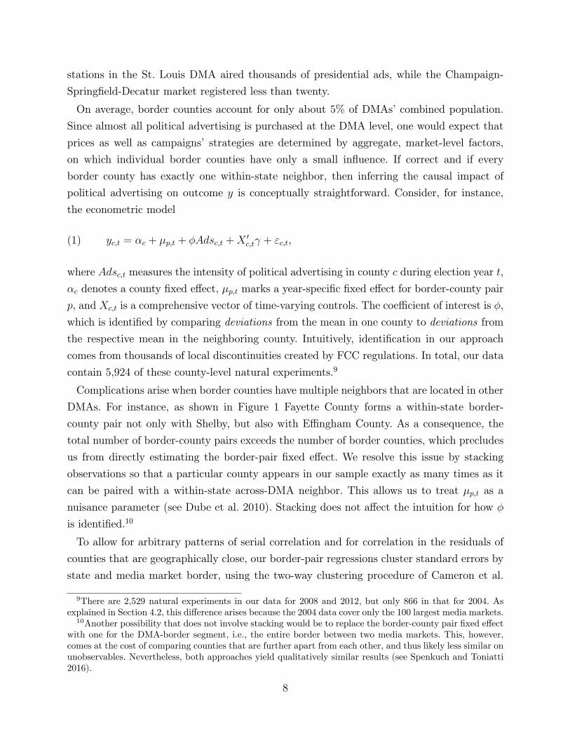
stations in the St. Louis DMA aired thousands of presidential ads, while the Champaign-

Springfield-Decatur market registered less than twenty.

On average, border counties account for only about 5% of DMAs’ combined population.

Since almost all political advertising is purchased at the DMA level, one would expect that

prices as well as campaigns’ strategies are determined by aggregate, market-level factors,

on which individual border counties have only a small influence. If correct and if every

border county has exactly one within-state neighbor, then inferring the causal impact of

political advertising on outcome y is conceptually straightforward. Consider, for instance,

the econometric model

(1) yc,t = αc + µp,t + φAdsc,t +X ′c,tγ + εc,t,

where Adsc,t measures the intensity of political advertising in county c during election year t,

αc denotes a county fixed effect, µp,t marks a year-specific fixed effect for border-county pair

p, and Xc,t is a comprehensive vector of time-varying controls. The coefficient of interest is φ,

which is identified by comparing deviations from the mean in one county to deviations from

the respective mean in the neighboring county. Intuitively, identification in our approach

comes from thousands of local discontinuities created by FCC regulations. In total, our data

contain 5,924 of these county-level natural experiments.9

Complications arise when border counties have multiple neighbors that are located in other

DMAs. For instance, as shown in Figure 1 Fayette County forms a within-state border-

county pair not only with Shelby, but also with Effingham County. As a consequence, the

total number of border-county pairs exceeds the number of border counties, which precludes

us from directly estimating the border-pair fixed effect. We resolve this issue by stacking

observations so that a particular county appears in our sample exactly as many times as it

can be paired with a within-state across-DMA neighbor. This allows us to treat µp,t as a

nuisance parameter (see Dube et al. 2010). Stacking does not affect the intuition for how φ

is identified.10

To allow for arbitrary patterns of serial correlation and for correlation in the residuals of

counties that are geographically close, our border-pair regressions cluster standard errors by

state and media market border, using the two-way clustering procedure of Cameron et al.

9There are 2,529 natural experiments in our data for 2008 and 2012, but only 866 in that for 2004. Asexplained in Section 4.2, this difference arises because the 2004 data cover only the 100 largest media markets.10Another possibility that does not involve stacking would be to replace the border-county pair fixed effect

with one for the DMA-border segment, i.e., the entire border between two media markets. This, however,comes at the cost of comparing counties that are further apart from each other, and thus likely less similar onunobservables. Nevertheless, both approaches yield qualitatively similar results (see Spenkuch and Toniatti2016).

8

(2011). Clustering also corrects for the correlation that is introduced by stacking.

4.2. Data Sources

We apply this estimation strategy to uniquely detailed data on the intensity of political

advertising during the 2004, 2008, and 2012 presidential campaigns. Information on the

broadcast of political advertisements is available through a cooperation between the Cam-

paign Media Analysis Group (CMAG) and the Wesleyan Media and Wisconsin Advertising

Projects (Fowler et al. 2015; Goldstein et al. 2011; Goldstein and Rivlin 2007). According to

CMAG, the data form a complete record of all political ads that aired on any of the national

television or cable networks.11 In 2004, the 100 largest media markets, or about 86% of the

U.S. population, are covered. For 2008-12, coverage was expanded to all 210 DMAs. The

CMAG data include timestamps for each ad, the sponsoring group (i.e., a candidate’s cam-

paign, the national party, independent interest groups, such as PACs, etc.), the candidate it

supported, as well as more detailed, human-coded information on its content.

As political advertisements air at all times of the day and during different programs, the

total number of ads that are broadcast in a particular market makes for a questionable mea-

sure of advertising intensity, i.e., the number of ads that people actually saw. To directly

gauge constituents’ exposure to political advertising, we use detailed viewership information

provided by The Nielsen Company. Nielsen is the market leader in television-audience mea-

surement. At the heart of Nielsen’s efforts is a proprietary technology that tracks the media

consumption of a representative cross section of households. Relying on metering devices

installed in about 30,000 households, Nielsen monitors which channel is being watched at

any particular point in time on all TVs in the home. In addition, each year the company

collects approximately 2 million week-long TV diaries. These data then form the basis of the

so-called Nielsen ratings, which are available by gender and age group for each DMA.

We measure advertising intensity in impressions per capita among voting-aged adults.

An impression is defined as one viewer being exposed to one commercial. Our metric of

advertising intensity thus corresponds to the number of ads seen by the average adult in a

particular DMA. Given that CMAG and Nielsen time stamps do not perfectly match, we

average the Nielsen-reported number of impressions (among all viewers age 18 and older)

over thirty-minute intervals, and assign the corresponding value to the particular instance

in which an ad aired. To assess aggregate presidential advertising, we focus on a 60-day

time window leading up to the election and, for each market, sum impressions over all local

11Small-sample audits have found that the CMAG data are highly correlated with invoice data fromtelevision stations. For example, in an audit of Philadelphia stations, Hagen and Kolodny (2008) report thatless than 2% of ads were missing from the CMAG sample.

9

broadcasts of all presidential ads, including those sponsored by the national parties and other

interest groups.12 In symbols, aggregate presidential advertising in media market d during

year t is defined as Adsd,t ≡∑k

∑Sk,d,ts=1 Imps18+s,k /Pop

18+d,t , where k indexes candidates, and

Sk,d,t denotes the total number of spots in support of candidate k that aired in that market

within 60 days before the election.13

We measure partisan advertising in the same way, except that we sum only over ads that

support a particular candidate–either through positive messaging related to the candidate or

through negative messaging directed at his opponent. Since Nielsen ratings are only available

at the DMA level, we assign the same advertising measures to all counties within a given

market. If viewing habits in border counties differ from those in the remainder of the media

market, then our advertising variable is likely to contain measurement error, which would

bias our estimates towards zero. Yet, we believe that the Nielsen data constitute the best

available source of information on how many potential voters viewed a particular spot.14

County-level information on the total number of voters, votes for each presidential can-

didate, write-ins, etc., come from the CQ Voting and Elections Collection (Congressional

Quarterly 2015). To calculate voter turnout, we combine these data with population esti-

mates from the U.S. Census Bureau. All individuals age 18 and older are considered potential

voters. While this broad categorization includes some who are ineligible to vote (e.g., felons

and non-U.S. citizens), it has the advantage of being robust to endogenous voter registration.

To obtain information on the observable characteristics of counties’ residents, we turn to

the Census Bureau and the Bureau of Labor Statistics. To measure election coverage by the

local press, we count the number of election-related articles in the Factiva database, weighted

by the respective newspapers’ circulation in a particular county. In addition, we use the slant

index of Gentzkow and Shapiro (2010) to proxy for newspapers’ political leanings. Data on

candidate appearances by media market come from Shaw (2007), Huang and Shaw (2009),

and FairVote.org. For more detailed information on the data as well as precise definitions of

all variables used throughout the analysis, see the Data Appendix.

12This includes ads sponsored by PACs and, in the post-Citizens United era, by Super PACs. Althoughindividual point estimates do, of course, vary, our results are qualitatively and quantitatively robust toexcluding these advertisements.13According to CMAG, approximately 0.5% (0.1%) of spots in 2008 (2012) aired on cable channels. Since

the Nielsen data do not contain information on the viewership of cable channels disaggregated by DMA,we exclude these ads from our calculations. Similarly, our baseline measure of advertising intensity doesnot account for spots that aired nationally on any of the major networks because the CMAG data containno information on national ads in 2004. In 2008 (2012), less than 0.2% (0.9%) of ads aired nationally. Therobustness checks in Appendix Tables A.9 and A.11 demonstrate that including national ads has virtuallyno effect on the estimated coefficients for the respective elections.14We have also experimented with other measures of advertising intensity and different time windows,

obtaining qualitatively very similar results (see Appendix Tables A.9 and A.11).

10

4.3. Descriptive Statistics & Tests of the Identifying Assumption

Combining all different sources, Table 1 displays summary statistics for our county-level

data set, by border-pair status. There is considerable variation in advertising intensity. The

average county in our data records 71 impressions per capita. In some areas, however, voting-

aged adults see over 450 spots, whereas other counties have virtually no presidential ads on

TV. Variation with respect to turnout and vote shares is also quite large.

Table 1 further shows that border counties are not perfectly representative of the United

States as a whole. Although turnout is broadly comparable across border and non-border

counties, the former are less populous and have lower median incomes. More important for

our purposes is whether, conditional on constituent characteristics, advertising intensity is

truly as good as random across media market borders. If so, then the estimates below recover

a local treatment effect. That is, we estimate the impact of political advertising on voters

who viewed a given number of ads only because they lived on either side of a DMA border.

Unfortunately, our identifying assumption that differences in advertising intensity are un-

correlated with differences in time-varying unobservables is fundamentally untestable. One

may be willing to judge its plausibility, however, by asking whether differences in observ-

ables predict differences in advertising. A correlation between political advertising and border

counties’ time-varying observable characteristics would raise concern about a similar corre-

lation with unobservables.

Table 2 provides suggestive evidence that this concern is not warranted. The results therein

are based on the estimator in equation (1), using different measures of political advertising

as outcomes. For ease of interpretation, all variables have been standardized, so that the

coefficients refer to the standard deviation change in advertising resulting from a standard

deviation increase in the regressor.

Regardless of which advertising measure we consider, few of the point estimates in Table 2

are economically large or statistically significant. In fact, for each specification a joint F -test

is unable to reject the null hypothesis that all coefficients are exactly equal to zero, with p-

values ranging from 0.349 to 0.655. Remarkably, observable characteristics explain less than

1% of the within-variation in the respective measure of advertising intensity.15

For a subset of thirty-one media markets we have also been able to obtain transcripts of

televised news shows ahead of the 2008 election. In Appendix B, we rely on these transcripts

to measure election coverage by local TV stations. Reassuringly, differences in news coverage

do not predict differences in political advertising. Moreover, Appendix D presents placebo

15In addition, we have used our border-pair estimator to regress each outcome on each covariate separately.Two out of fifty coefficients are statistically significant at the 5%-confidence level, and the distribution ofp-values is statistically indistinguishable from a uniform distribution (cf. Appendix Figure A.5).

11

tests asking whether future advertising “affects” current election results. It does not. Of the

81 point estimates in Appendix Table A.7, only four are statistically significant, most of

which have the “wrong” sign.

Our interpretation of these results is that differences in political advertising between bor-

der counties are essentially random. We hasten to add, however, that it is impossible to

definitively prove the validity of our identifying assumption.

5. Political Advertising and Election Results: Empirical Evidence

5.1. Political Advertising and Turnout

We now explore the effect of total political advertising on voter turnout. Pooling over the

2004—12 presidential elections, Table 3 presents the results, relying on our sample of stacked

border-pair counties.16 The simple OLS estimate in column (1) suggests that an additional

ten impressions per capita raise voter turnout by almost 0.21 percentage points. Put differ-

ently, a standard deviation increase in presidential advertising is associated with an increase

in turnout of about 2.2 percentage points. Adding county fixed effects to control for time-

invarinat unobservables reduces the point estimate by more than a third. Yet, it remains

statistically significant and sizeable. Based on the evidence presented so far, it would appear

that political advertising leads to a nontrivial increase in voter engagement.

Column (4) implements our cross-border pair estimator in equation (1). Remarkably, com-

paring only neighboring counties reduces the coefficient on total advertising to near zero. The

sharp reduction in the point estimate between columns (2) and (4) suggests that campaigns

advertise more in areas and years in which citizens are more likely to vote anyway. Since

counties that are geographically close tend to experience similar shocks, our border-pair

estimator is able to account for this confound, while more naıve approaches cannot.

Column (5) additionally controls for all time-varying covariates shown in Table 2, all non-

presidential political advertising as well as candidate visits as a proxy for campaigns’ ground

operations. The last column in Table 3 controls for the lagged dependent variable in lieu

of county fixed effects. This specification may be more appropriate if campaigns directly

base their advertising decisions on the outcome of the last election. Moreover, the model

in column (6) lets us split the data by year in order to estimate the impact of political

advertising separately for each election (see Appendix D).

The results in the lower panel of Table 3 are based on the same specifications as those

in the upper one, but allow for heterogeneity in the impact of “positive” and “negative”

16In Appendix Table A.8, we show that estimates for the sample of all counties with available advertisingmeasures are qualitatively and quantitatively very similar to those in columns (1)—(3) of Table 3.

12

advertising.17 Although estimates that allow for the effect to vary by tone are less precise,

they are almost equally close to zero. All in all, there is little to no evidence to conclude that

political advertising has a meaningful impact on aggregate turnout.18

In the appendix, we probe the robustness of our findings with respect to the weighting

scheme, different measures of advertising intensity, and various time windows before the

election (cf. Table A.9). We also investigate how the results vary across years. Broadly

summarizing, our robustness checks produce estimates that tend to be close to zero and

statistically insignificant. In particular, we obtain almost identical results when we reweight

border-pair counties by the inverse number of times that they appear in our stacked data

set. Our results are also qualitatively robust to restricting attention to border-pairs that

contain less than 5%, or even 2%, of the respective DMAs’ combined population. We find

this reassuring, as our identifying assumption is most plausible in cases where border counties

are highly unlikely to affect campaigns’ decisions.

Further, our point estimates remain nearly unaffected when we focus on county pairs

that are (almost) entirely contained within the same congressional districts, and we find

similar effect sizes in battleground and non-battleground states. In the former, campaigns’

unobserved ground operations may pose a serious threat to our identification strategy. The

latter set of states, however, remains typically untreated, as finite resources force campaigns

to focus their mobilization efforts. Observing qualitatively similar effects in both sets of

states suggests that campaigns’ ground operations are likely not a significant confounder.19

A remaining worry is measurement error in advertising intensity. Although our measure of

advertising is likely more precise than any in the literature, we cannot rule out that viewing

habits in border counties differ from the respective market average, or that a nontrivial

number of border-county households receive their television signal from the “wrong” DMA.

In 2010, for instance, about 9.5% of U.S. households relied on terrestrial antennae for their

television programming (Nielsen 2011). If a nontrivial number of households watches TV

stations from a neighboring DMA, then our advertising measure overstates the true difference

in treatment intensity, leading to estimates that are biased toward zero.

Under some assumptions, however, it is possible to gauge the severity of the bias. Suppose

17All evaluations of advertisements’ tone are due to human coders of the Wesleyan Media and WisconsinAdvertising Projects. See Freedman and Goldstein (1999) for a detailed description of the coding process.18A clear limitation of our approach is that the estimator in equation (1) imposes constant marginal effects.

Although we find that this is a reasonable assumption given the range of our data (see Appendix C), wecannot completely rule out potentially nontrivial macro effects of advertising on turnout.19Also, if local campaigning increases turnout, and if campaigning is positively correlated with advertising

intensity, then our estimates of the impact of political ads on turnout should be upward biased. The factthat the results are close to zero is consistent with the view that local campaigning does not systematicallyvary across media market borders within the same state.

13

that a fraction of q randomly chosen households receive their television signal from the

neighboring DMA. If these households were to exclusively watch programs originating in the

“wrong” market, then the actual, unattenuated effect of political advertising would equal

(2) φ∗ =1

1− 2qφ,

where φ denotes the original estimate.20 To get a sense of reasonable values for q, consider

the case in which border-county households have the same propensity to rely on antenna TV

as the national average, and further assume that one in two antenna households obtain their

television signal from the “wrong” DMA. In such a case, q ≈ 0.05 and φ∗ ≈ 1.1φ. Even if

households in border counties were twice as likely as the national average to watch antenna

TV, and if every single antenna household watched only programs that originated in the

neighboring DMA, i.e., even if q ≈ 0.2 and φ∗ ≈ 1.67φ, the true effect of political advertising

on voter turnout would still be only a fraction of the variables’ correlation in the raw data.

We, therefore, conclude that political advertising has at best a small impact on aggregate

turnout.

This result is well aligned with Ashworth and Clinton (2007) and Krasno and Green (2008),

who argue that advertising is ineffective at engaging the electorate. The main difference

between our estimates and theirs is that ours are precise enough to rule out moderately large

effect sizes. In our preferred specification in column (6) of Table 3, the 95%-confidence interval

ranges from −0.004 to 0.036 percentage points. By contrast, Ashworth and Clinton (2007)

estimate that having seen “many” campaign advertisements increased survey respondents’

intent to vote by 0.7 percentage points, with a 95%-confidence interval of [−15.7, 17.1].

Krasno and Green (2008) use gross ratings points (GRPs) to measure advertising intensity.

Controlling for the lagged dependent variable and state fixed effects in a cross-section of 128

DMAs, they find that the average TV viewer seeing ten additional ads increases turnout by

0.05 percentage points. The 95%-confidence interval on their coefficient ranges from −0.06

to 0.16, which narrowly excludes the naıve OLS estimate.

5.2. Political Advertising and Vote Shares

The evidence above suggests that our empirical approach is capable of distinguishing between

true effects and relationships that are spurious. We now use it to study advertising’s impact

20To derive (2), let turnout in border counties A and B be denoted by yA and yB , respectively, and letmeasured advertising be given by AdsA and AdsB . Abstracting from differences in covariates, the estimatedeffect of advertising equals φ = (yA − yB) / (AdsA −AdsB). The actual amount of advertising seen by theconstituents in A and B, however, is Ads∗A = (1 − q)AdsA + qAdsB and Ads∗B = (1 − q)AdsB + qAdsA. It

follows that φ∗ ≡ (yA − yB) / (Ads∗A −Ads∗B) = φ/(1− 2q).

14

on vote shares.

Table 4 focuses on the impact of partisan differences in advertising on differences in vote

shares. We define both variables so that positive values indicate an advantage of the Demo-

cratic candidate over his Republican opponent, i.e., ∆Ads ≡ AdsD−AdsR and ∆v ≡ vD−vR.

As in the preceding analysis, column (1) shows a strong, positive raw correlation between de-

pendent and independent variable. The next two sets of columns add county fixed effects as

well as controls for demographics, economic conditions, candidate visits, newspaper report-

ing, and non-presidential advertising. This decreases the estimated correlations substantially,

but does not render them meaningless.

Columns (4)—(6) implement our border-county pair identification strategy. Comparing only

neighboring counties leads to a further reduction in the coefficients. At the same time, the

estimated coefficients become much more precise. Taking the point estimates in columns

(4)—(6) at face value, a standard deviation increase in the partisan difference in presidential

advertising–the equivalent of potential voters seeing an additional twenty-one spots for the

Democratic candidate rather than the Republican one–increases the Democratic candidate’s

vote share by about 0.49 to 0.67 percentage points relative to that of his Republican oppo-

nent. It, therefore, appears that political advertising has a nonnegligible impact on election

results, especially if one suspects that measurement error in advertising intensity attenuates

the coefficients.

In Appendix D, we present results from a battery of sensitivity and robustness checks.

Although the point estimates for the 2004 election are smaller than those for 2008 or 2012,

the baseline estimates for these years are statistically indistinguishable from each other

(p = 0.210). This is noteworthy because 2004 and 2008 predate the analytics revolution in

electioneering, after which narrowly targeted campaign activities may pose a problem for our

identification strategy. It is also reassuring that the estimated effect of political advertising

on vote shares remains qualitatively the same when we limit the sample to counties whose

populations comprise less than 2% of the respective media markets, i.e., counties for which

we believe our approach to be the most credible. Interestingly, there is no evidence to suggest

that advertising was differentially effective in battleground and non-battleground states, or

across states with clear partisan leanings. We do, however, find evidence that political ads

exerted greater effects on less educated populations. Splitting our sample into counties above

and below the median share of college graduates yields point estimates (standard errors) of

0.231 (0.063) and 0.436 (0.081), which are statistically distinguishable at the 5%-confidence

level (cf. Appendix Table A.11).

15

5.3. Instrumental Variables Estimates

As a further robustness check, Tables 5 and 6 present results from an instrumental variables

strategy in the spirit of Krasno and Green (2008) and Huber and Arceneaux (2007). Given

that campaigns tend to focus their resources on states in which the race is likely to be close,

these authors observe that some voters are exposed to more political ads than others simply

because they happen to live in a DMA that partially overlaps with a battleground state.

Going back to the example in Figure 1, Illinois voters living in the St. Louis media market

saw more political ads than those in the Champaign-Springfield-Decatur DMA at least in

part because the former market also serves voters in Missouri, where the 2008 election was

highly competitive. We build on this insight and combine it with our border-pair approach.

Comparing neighboring counties within the same state, Table 5 demonstrates that the

share of a media market’s population that is contained in a battleground state is, indeed, a

strong predictor of advertising intensity. Voters in noncompetitive states see more presiden-

tial ads on TV when their own DMA overlaps to a greater extent with a battleground state

than the neighboring market. Conversely, individuals in competitive states see fewer political

ads when the share of non-battleground voters who reside in the same DMA is larger.21 Im-

portantly, advertising in support of the Democratic candidate is more responsive to DMAs’

“battleground population share” than that supporting the Republican one. Leading up to

the 2008 election, Barack Obama and John McCain pursued different strategies (see, e.g.,

Franz and Ridout 2010). Not only did the former campaign advertise more than the latter,

but it also put greater emphasis on highly competitive states, such as Florida, North Car-

olina, Virginia, and Nevada. As a consequence, our instrument is not only predictive of total

presidential advertising but also of partisan differences therein.

Table 6 displays reduced form as well as two-stage least squares estimates of the impact

of political advertising on turnout and vote shares. Intuitively, the identifying assumption is

that differences in the extent to which neighboring DMAs overlap with battleground states

are uncorrelated with time-varying differences in unobserved determinants of individuals’

voting decisions. If this exclusion restriction is, indeed, satisfied, then the IV estimates have

a causal interpretation.

Relative to their counterparts in Tables 3 and 4, three out of the four two-stage least-

squares coefficients are larger in magnitude but also less precisely estimated. With p-values

of 0.081 and 0.047 the estimated effect on vote shares remains marginally significant. Based

on these estimates, we continue to conclude that political advertising has no appreciable effect

on overall turnout, but skews the outcome of the election in favor of whichever candidate

21As explained in the Data Appendix, we define battleground states according to the classification byRealClearPolitics.com six to eight weeks prior to the election.

16

advertises more.

Notwithstanding the imprecision of the IV results, the estimates in Table 6 are useful for at

least two reasons: (i) they correct for attenuation bias due to measurement error in advertis-

ing intensity, and (ii) they help to address an array of potential confounds. Shapiro (2018),

for instance, documents cross-media market differences in advertising for antidepressants,

and there may well be other, unobserved variables that also vary across DMA borders. For

some unobserved factor to bias our IV estimates, it would not only have to affect the election

result in the respective county, but it would also have to be systematically correlated with

the extent to which the remainder of the media market overlaps with battleground states.

Given that DMA borders were drawn by The Nielsen Company based on historical viewing

patterns, most unobserved determinants of election outcomes seem a priori unlikely to be

correlated with whether or not other counties in the same DMA belong to a competitive

state.

5.4. Partisan Effects

Next, we return to our workhorse empirical model and investigate heterogeneity in the ef-

fect of Democratic and Republican advertising. Table 7 presents results for vote shares that

are defined relative to the entire voting-aged population. This frees us from having to ad-

just for turnout when we calculate persuasion rates in Section 7. More importantly, using

population-based vote shares as dependent variables allows for the theoretical possibility

that one candidate’s advertising has no effect on the (absolute) support for his opponent.

Although some of the estimates in Table 7 are small and lack statistical significance, as

a whole the evidence suggests that own advertising increases support for the respective

candidate, while a rival’s spots are detrimental to it. Of course, this pattern would emerge

automatically had we used regular two-party vote shares as outcomes. With vote shares

defined relative to the entire voting-eligible population, however, there is no mechanical

reason for the apparent symmetry in the estimates.

One plausible explanation–especially in light of our null result with respect to aggregate

turnout–is that the persuasive effects of political advertising operate primarily on the in-

tensive margin. That is, advertising might convince those who would have gone to the polls

anyway to vote for one candidate rather than the other. Another possible rationalization is

that political advertising works on the extensive margin by affecting who turns out to vote.

For instance, advertising by the Democratic candidate might mobilize Democratic support-

ers or left-leaning moderates all the while deterring voters who would choose his Republican

opponent. In the aggregate such compositional effects might happen to offset each other,

which would explain why there appears to be no meaningful impact on overall turnout.

17

6. Political Advertising and the Partisan Composition of the Electorate

Using only aggregate data there is little hope to credibly distinguish between these two ex-

planations. In order to shed at least some light on the mechanism behind our main result, we

have acquired individual-level voter-registration data for the lower forty-eight states and the

District of Columbia. The Help America Vote Act of 2002 requires that all states maintain a

single, computerized voter-registration list that is regularly updated by removing individuals

who are deceased or ineligible, as well as duplicate entries in accordance with the National

Voter Registration Act of 1993. The resulting lists include voters’ residential address, date

of registration, and turnout history.

For a subset of individuals, we also have information on date of birth, gender, and party

affiliation. In particular, thirty-nine states’ voter-registration files have either a dedicated

“party” field, or they contain enough information to determine in which party’s primary (if

any) a given individual participated. We identify individuals as a “registered Democrat” or

“registered Republican” if the state lists them as such, or if they voted in the respective

party’s primary. Voters who are not officially affiliated with any of the two major parties

and did not participate in one of their primaries are classified as “other.”22

6.1. Empirical Approach

To assess whether political advertising leads to changes in the partisan composition of the

electorate, we geocode all addresses and use the information on voters’ precise locations

relative to DMA borders in a regression discontinuity (RD) design (Lee and Lemieux 2010;

Thistlethwaite and Campbell 1960). That is, we compare turnout among registered De-

mocrats and Republicans who live on opposite sides of media market borders. Specifically,

we are interested in whether the partisan difference in turnout varies discontinuously at

the border. In Section 6.3, we show that advertising’s impact on the partisan difference in

turnout is a key parameter in assessing the importance of the compositional channel.

As above, we define the partisan difference in advertising as the number of impressions

per capita in support of the Democratic candidate minus that for his Republican opponent.

We then say that a particular voter lives “left” (“right”) of the border if partisan differences

in presidential advertising are smaller (larger) in the DMA in which she resides than in the

neighboring one.

Interpreting our RD setup through the standard instrumental variables framework (Hahn

et al. 2001), we calculate the impact of partisan differences in political advertising on partisan

22We also classify as “other” individuals whose recent vote history indicates that they had participated indifferent parties’ primaries.

18

differences in turnout by forming the Wald estimator:

(3)

∆(tD−tR) =lim

mi→0+(E [ti|i = D,mi]− E [ti|i = R,mi])− lim

mi→0−(E [ti|i = D,mi]− E [ti|i = R,mi])

limmi→0+

E [AdsD − AdsR|mi]− limmi→0−

E [AdsD − AdsR|mi].

Here, ti is an indicator for whether individual i turned out to vote, and mi denotes her

distance to the nearest media market border, with negative values assigned to voters who

live on the “left.” AdsD and AdsR are the number of Democratic and Republican impressions

per capita, respectively.

While our voter-registration data are well suited to estimate the numerator of equation (3),

our advertising measure varies only at the DMA level and is, therefore, likely to overstate

the true difference in the advertising exposure of voters in the vicinity of media market

borders. This is because individuals who reside close to the border may be more likely to use

terrestrial antennae to watch TV stations from the “wrong” DMA. If true, then our Wald

estimates are biased towards zero.

Even in the absence of this issue, it bears emphasizing that RD methods can only identify

local average treatment effects (Imbens and Angrist 1994). That is, we estimate the impact

of political advertising on the set of voters who live close to media market borders. Since

identification comes from only a small percentage of the electorate, the results below may

not generalize to the U.S. population as a whole.

At the same time, our RD strategy has at least two advantages. First, constituents’ ex-

posure to radio advertising and campaigns’ ground operations is unlikely to exhibit a sharp

discontinuity at within-state media market borders and, therefore, should not bias the RD

estimates. Second, identification in our setting actually comes from differences in discon-

tinuities.23 Thus, unlike traditional RD designs, our estimation strategy allows for other

variables to vary discontinuously across media market borders, as long as these variables do

not differentially affect turnout among Republicans and Democrats (see Grembi et al. 2016

for a discussion of identification in the DRD design).

In the appendix, we present evidence consistent with the more demanding assumption

that there are no discontinuities in other, predetermined variables. Briefly, to check for

irregularities in the running variable, we look at population density in the vicinity of DMA

23To see this, rearrange the numerator of equation (3) to

(lim

mi→0+E [ti|i = D,mi]− lim

mi→0−E [ti|i = D,mi]

)−(

limmi→0+

E [ti|i = R,mi]− limmi→0−

E [ti|i = R,mi]

). The first term denotes the discontinuity in turnout among

Democrats, while the second one gives the discontinuity in turnout among Republicans.

19

borders. Based on the evidence in Figures A.11 and A.12, there is little reason to suspect

that individuals in our sample are more likely to settle on one side of the border than on the

other. Similarly, we find no evidence of meaningful differences in how long voters on either

side of the border have been registered at their current address (cf. Table A.13), which helps

to ameliorate concerns about selective attrition.

We also test for discontinuities in voters’ age, gender, party affiliation, and turnout in

other elections (cf. Tables A.14—A.17). The point estimates are small, and often of vary-

ing sign. In the same vein, Table A.18 shows that partisan differences in non-presidential

political advertising do not systematically vary “left” and “right” of the DMA border. In

particular, the sign of the estimated discontinuity is an order of magnitude smaller than that

in Figure 2 below. Appendix Tables A.19—A.21 test for systematic differences in newspaper

circulation, local-school expenditures, and property values, none of which appear to exhibit

a discontinuity.24

6.2. RD Estimates

Table 8 presents basic, descriptive statistics for our voter-registration data. Given that most

states did not create statewide, digital voter-registration databases until after 2004, turnout

histories for earlier years tend to be incomplete.25 We, therefore, focus on the 2008 and 2012

presidential elections. Another important limitation of our data is that we only observe the

current address at which someone is registered. Since we cannot retrospectively ascertain

individuals’ place of residence, we restrict attention to cases in which a voter’s registration

predates the respective election. For the average individual in our sample, the straight-line

distance between her residence and the nearest media market border is about 71 kilometers.

Eighteen percent, however, live within 25km of a DMA border; and about two percent reside

within 5km.

Pooling over all partisans living within 25km of a media market border, Figures 2 and

3 depict our main RD results. Figure 2 shows raw averages for the partisan difference in

advertising within 2.5 kilometer intervals on either side of the border, i.e., the denominator

in equation (3). Figure 3 does so for the numerator, the partisan difference in turnout.

By construction, media market borders feature a large discontinuity in partisan advertis-

24Data on these outcomes come from the Alliance for Audited Media, the National Center for EducationStatistics, and CoreLogic/DataQuick. See the Data Appendix for details.25In Wisconsin, for instance, voter registration and participation lists were maintained by municipal clerks,

and municipalities with populations of 5,000 or less were exempt from such record keeping. While the stateof Wisconsin does not include turnout information prior to 2006 with its official voter registration data,other states do. These lists provide an accurate picture of turnout in earlier election cycles only where locallymaintained records were thoroughly integrated into the statewide database. In our data, turnout numbersfor 2004 are often substantially lower than what would be expected based on official statistics.

20

ing.26 On average, the size of the gap is a bit more than twenty impressions per capita. That

is, voting-aged adults to the “right” of the border see about twenty additional ads favoring

the Democratic candidate. Partisan differences in turnout also exhibit a discontinuity. Reg-

istered Democrats living just to the “left” of the border are between five and six percentage

points less likely to go to the polls than their Republicans counterparts, but the gap narrows

by almost two percentage points among those living just on the other side. The evidence in

Figures 2 and 3, therefore, suggests that partisan differences in political advertising induce

changes in the partisan composition of the electorate.

Based on the graphical analysis, one would conclude that an increase in the partisan

difference in advertising by ten impressions per capita raises turnout of registered Democrats

by nearly one percentage point relative to their Republican counterparts. Of course, this

simple analysis is subject to a number of limitations. First, there is no a priori reason for

why the true functional relationship between the running variable and differences in turnout

would need to be linear. Second, Figures 2 and 3 pool over different natural experiments and

may, therefore, be affected by unobserved spatial heterogeneity. In what follows, we probe

the results of the graphical analysis by using nonparametric techniques (Hahn et al. 2001;

Porter 2003).

Table 9 presents the results. The estimates in the upper panel refer to the numerator of the

Wald estimator and are based on the following “differences in discontinuities” specification:

yi,p,s,e = αp,s,e + τ1 [p = D]× 1 [mi > 0] + δ1 [mi > 0](4)

+ glp (mi)× 1 [mi < 0] + grp (mi)× 1 [mi > 0] + ξi,p,s,e,

where yi,p,s,e is an indicator variable for whether voter i, who is a registered supporter of

party p ∈ {D,R} and lives close to border segment s, went to the polls in election e. glp (·)and grp (·) are flexibly specified, party-specific polynomials of distance, which are allowed to

differ on either side of the threshold. To control for unobserved spatial heterogeneity, we

divide every DMA border into segments of up to 10km length and include αp,s,e, a party-

and election-specific fixed effect for each of them. The parameter of interest is τ .

All estimates use a rectangular kernel with the respective bandwidth indicated at the top

of each column. Going from left to right, the bandwidth increases from 500 meters to 5

kilometers, with the last column relying on 10-fold cross-validation for bandwidth selection

(Ludwig and Miller 2005). Successive rows use higher-order polynomials to approximate glp (·)and grp (·).

26The fact that the average number of impressions varies across bins on either side of the border is due todifferences in the spatial distribution of voters across DMAs.

21

Our nonparametric estimates of τ range from 0.9 to 2.3 percentage points, which is roughly

inline with the graphical analysis. Appendix Table A.22 decomposes the point estimates into

changes in turnout among registered Democrats and Republicans. The sign pattern suggests

that registered Democrats are more likely to vote–even in absolute terms–the more the

Democratic candidate advertises relative to the Republican one. For registered Republicans

we tend to observe the opposite effect, though the coefficients are more variable from one

specification to the next.

One, admittedly speculative, explanation for why political advertising may also have de-

mobilizing effects is that a substantial share of ads are negative. As in the experiments of

Ansolabehere and Iyengar (1995), attack advertising may diminish the psychological ben-

efits of turning out to support a particular candidate. Unfortunately, RD estimates that

attempt to disentangle the effects of positive and negative advertising are too imprecise to

draw any conclusions. As a whole, however, the reduced form evidence suggests that partisan

differences in presidential advertising alter the partisan composition of the electorate.

The lower panel of Table 9 uses two-stage least squares to implement the Wald estima-

tor.27 To facilitate comparisons with the results in the remainder of the paper, we scale

the coefficients so that they refer to the impact of 10 impressions per capita. The resulting

Wald estimates range from 0.4 to 1.2 percentage points. The median coefficient is about

0.8 percentage points.28 Based on this evidence, we conclude that political advertising has a

detectable impact on the partisan composition of the electorate.

6.3. Assessing the Importance of Compositional Changes

How important are these compositional shifts? Under the assumption that registered par-

tisans are more likely to vote for their own party’s candidate than for his competitor, we

can assess how much of the estimated effect of political advertising on vote shares can be

explained by changes in the partisan composition of the electorate alone.

Formally, let candidates’ vote shares be given by vD and vR, and assume that, conditional

on going to the polls, registered partisans vote for the candidate of their own party with

probability π > 0.5. With vD and vR defined relative to the entire voting-eligible population,

the following accounting identity must always hold:

vD − vR = [πtDsD + (1− π) tRsR + ωtOsO]− [(1− π) tDsD + πtRsR + (1− ω) tOsO] .

27For completeness, Appendix Table A.24 presents the “first stage” estimates, i.e., the denominator of theWald estimator.28Replacing the border segment fixed effect in equation (4) with one for every individual and thus exploiting

only the time series variation in our data yields Wald estimates between 0.4 and 0.6 percentage points.

22

Here, tp denotes turnout among supporters of party p, sp is their population share, and ω

stands for the likelihood that “others” will vote for the Democratic candidate. Noting that

sD ≈ sR among voters close to media market borders, we can decompose changes in the

partisan difference in vote shares into

∆ (vD − vR) ≈ (2π − 1) s∆ (tD − tR) + (2ω − 1) (1− 2s) ∆tO(5)

+ 2s (tD − tR) ∆π + 2 (1− 2s) tO∆ω

+ 2s∆ (tD − tR) ∆π + 2 (1− 2s) ∆tO∆ω.

The first term on the right-hand side of equation (5) denotes the contribution of changes in

turnout among partisans, while the second one refers to turnout of unaffiliated individuals.

The terms in the row beneath constitute the effect of changing preferences (i.e., changes in

the probability of voting for a particular party, conditional on going to the polls), while the

ones in the third row refer to the interaction between shifts in both preferences and turnout.

To assess the importance of the compositional channel, suppose that political advertising

has no effect on preferences and beliefs, and that it leads to no changes in turnout among

unaffiliated voters. Equation (5) then simplifies to

(6) ∆ (vD − vR) ≈ (2π − 1) s∆ (tD − tR) .

Assuming that Democrats and Republicans each represent one-third of the population (i.e.,

s = 0.33), and relying on the range of the Wald estimates for plausible values of ∆ (tD − tR),

Figure 4 plots the right-hand side of equation (6) as a function of π. For comparison, in

Table 7 we estimated that political advertising raises the partisan difference in vote shares

by 0.165 percentage points (horizontal line).

Naturally, as the fraction of partisans who vote for the candidate of their own party in-

creases, differences in turnout explain a greater proportion of the difference in vote shares.

To get a sense of plausible values for π, we turn to the American National Election Survey

(ANES). Among other questions, the 2008—2009 ANES Panel Study elicited respondents’

vote choice in the 2008 presidential election as well as their self-declared party affiliation

prior to election day. Respondents could identify as “strong Republican/Democrat,” “not

very strong Republican/Democrat,” “independent Republican/Democrat,” or as truly “in-

dependent.” Almost 86% of those who self-identified as “strong” or “not very strong” De-

mocrats later indicated that they also voted for Barack Obama. Conversely, about 92% of

self-declared Republicans supported John McCain. Although self-reported votes are noto-

riously unreliable indicators of actual choices, the available evidence suggests that π may

23

exceed 0.8. If correct, then changes in turnout among partisans can explain most, if not all,

of the estimated impact of advertising on vote shares.

6.4. Sensitivity and Robustness Checks

We have conducted an extensive set of sensitivity and robustness checks. To conserve on

space, the corresponding results are presented in Appendix Tables A.25—A.29. The evidence

in these tables indicates that our RD estimates are robust to controlling for voters’ observable

characteristics and advertising related to non-presidential races. We also obtain qualitatively

and quantitatively similar results when we restrict attention to the set of voters for whom

our geocodes are the most precise, i.e., those for whom the geocoding procedure is able to

locate voter’s street address, or when we only compare voters on opposite sides of media

market borders within the same congressional district.

To assess the impact of measurement error in advertising intensity, we turn to the FCC’s

Significantly Viewed List (FCC 2005). In 2005, the FCC issued an updated, comprehensive

assessment of all media markets in the United States. In particular, it released a list of

counties where out-of-market broadcast stations have a nontrivial viewership. In Appendix

Table A.29, we restrict our sample to voters who live in counties where no out-of-market

station appears on the FCC’s list. Consistent with the idea that measurement error intro-

duces attenuation bias, the majority of the resulting Wald estimates are larger than their

counterparts in Table 9. At the same time, we note that the smaller sample size leads to

standard errors that make any quantitative comparisons highly speculative.

6.5. Total Presidential Advertising and Turnout

So far we have restricted attention to registered partisans, as this has allowed us to assess

the importance of the compositional channel. We now provide a partial test of the hypothesis

that political advertising also transmits useful information.

Theoretical work that relates the quality of voters’ information to turnout typically con-

cludes that, in a given election, informed individuals are more likely to vote than the unin-

formed (see Feddersen and Pesendorfer 1996, 1999). The intuition behind this result is that

informed voters are less likely to make a mistake by choosing the ex post worse candidate.

If information does, indeed, increase turnout, and if political advertising does contain new

information, then we would expect that independent voters who see more political ads on

TV are more likely to turn out than those who see fewer spots.

We test this hypothesis using a slight modification of our RD design. Instead of assigning

a particular voter to either side of the DMA border according to the partisan difference

in presidential advertising, we do so based on whether total presidential advertising in her

24

DMA exceeds that in the neighboring one. Despite a large discontinuity in total advertising

(cf. Figure 5), the Wald estimates in the upper panel of Table 10 suggest that unaffiliated

voters who are exposed to more political ads are no more likely to turn out.

For completeness, Figure 6 and the lower panel of Table 10 present results for turnout

among all voters. Again, there is no evidence of a positive discontinuity at the DMA border,

which implies that our previous finding of a minimal effect of presidential advertising on

overall turnout is not an artifact of using aggregate data. While we find no evidence in

favor of the idea that political advertising endows voters with useful information, we readily

acknowledge that a better test would also consider actual votes.

In sum, our RD results suggest that political advertising induces changes in the partisan

composition of the electorate, which offset in the aggregate. To be clear, we do not claim that

changes in the partisan composition of the electorate will always exactly cancel out. However,

in an environment with two candidates who have roughly the same number of supporters,

and if ads have both mobilizing and demobilizing effects, one would expect a considerably

smaller net impact–especially when both campaigns advertise in similar proportions.

7. Discussion

To put the estimated effect of political advertising on vote shares into perspective, we follow

DellaVigna and Kaplan (2007) and calculate persuasion rates. Intuitively, the persuasion

rate measures the percentage of individuals who changed their behavior in response to being

exposed to a particular message. Given that different studies use different left- and right-

hand side variables, and in light of the fact that the share of individuals who are susceptible

to being persuaded varies from one setting to the next, it is useful to rescale effect sizes in

this way in order to make them more comparable. Formally, the persuasion rate is defined

as

(7) fp =1

1− yp∆yp

∆Adsp,

where ∆yp/∆Adsp approximates the change in the outcome of interest induced by seeing

additional advertisements in support of candidate p, and 1− yp is the fraction of individuals

who may be swayed by the respective candidate’s message.29

We take the outcome of interest to be the partisan difference in vote shares defined as a

percentage of the entire voting-aged population. Defining y in this way has two advantages.

First, it is not necessary to adjust for turnout. Second, we capture advertising’s positive

29Appendix E derives equation (7) formally. At the request of a referee, we note that fp is a local measureof the effectiveness of advertisements. With a finite population the marginal impact of a particular messagemust eventually decline to zero.

25

effect on own vote shares as well as any negative impact on the support for political rivals.

If the Democratic candidate, for instance, is purely office motivated, then he should be

indifferent between one more vote for himself and one less for his Republican competitor.

As a consequence, 1− yD, the target audience for his ads, includes everybody who does not

already vote for him, i.e., everybody who would either abstain or vote for his opponent.

First, we calculate the persuasion rate of one additional spot, given the observed overall

level of advertising and candidates’ equilibrium vote shares. To proxy for ∆yp/∆Adsp, we

rely on the point estimates in column (8) of Table 7, divided by ten to account for the fact

that the coefficients refer to the impact of ten impressions per capita. With the respective

numbers in hand, the persuasion rate (and its standard error) is fD ≈ 0.03% (0.004%) for

Democratic spots, and that for Republican advertising equals fR ≈ 0.01% ( 0.005%).30

Next, we consider the share of potential voters who changed their behavior in response to a

candidates’ total advertising. To proxy for yp in the absence of advertising by the respective

candidate, we use the results in columns (2) and (5) of Table 7 and predict counterfactual

vote shares. ∆yp/∆Adsp is, again, given by the appropriately scaled coefficients in column

(8) of the same table. The resulting persuasion rates are fD ≈ 1.1% (0.18%) and fR ≈ 0.4%

(0.14%).31

Regardless of whether we calculate the persuasion rate for a single spot or for all of a

candidates’ combined advertising, the respective numbers are only a fraction of the persua-

sion rates reported in the literature (cf. DellaVigna and Gentzkow 2010). Our findings are,

therefore, consistent with the theoretical prediction that, as long as journalists are less likely

to be biased than campaigns, the effect of partisan advertising ought to be smaller than

that of slanted news (e.g., Knight and Chiang 2011). Assuming constant returns to scale, for

political advertising to be similarly persuasive as being exposed to FOX News (f = 11.6)

or to “alternative facts” during the 2017 French presidential election (f = 10.8, cf. Barrera

et al. 2018), a viewer would need to see about 500 spots. Within two months before the

2012 elections, only one media market registered a similarly high number of impressions per

voting-aged adult. In 2004 and 2008 none did.

However, in light of the large number of viewers who see at least some political ads on

TV, a more relevant metric might be advertising’s aggregate impact. Within 60 days leading

up to the 2008 presidential election, the average voting-aged citizen saw about 45 spots in

support of Barack Obama and almost 30 ads favoring John McCain. According to the U.S.

Census Bureau, about 206 million Americans were eligible to vote that year (File and Crissey

30To account for clustering at the state level, standard errors are calculated using the block bootstrap.31It is important to note that these numbers are based on Nielsen ratings data, which do not correct for

viewer inattention during commercial breaks. Persuasion rates adjusted for inattention may well be higher.

26

2012), which, together with the numbers above, implies that political advertising affected

about 2.2 million voting decisions. Naturally, the effects of Democratic and Republican ads

will partially offset each other, resulting in a smaller net impact. Still, simply eliminating the

partisan difference in advertising by reducing the number of impressions in favor of Barack

Obama to the same level as those for John McCain would have narrowed the difference in

votes by more than half a million. While this would not have made much of a difference in

2008, in years in which the election is close a similar sized shift might well decide the overall

outcome of the race.

To put the effectiveness of political advertising into perspective, we note that, leading up

to the general election, Obama and McCain were estimated to have spent a combined $366

million on TV ads (New York Times 2008), which implies a cost per persuaded voter of

about $170. Experimental evidence from get-out-the-vote studies suggest that direct mail or

high-quality commercial phone banks generate an additional vote at a cost of about $100

to $200 (see, e.g., Green and Gerber 2015). Phone banks staffed with volunteers or door-

to-door canvasing campaigns mobilize supporters at substantially lower cost–about $30

to $50 per vote–but are inherently limited in scale. Based on these back-of-the-envelope

calculations, political advertising appears to be roughly as effective as other scalable modes

of electioneering.

8. Concluding Remarks

In this paper we study the impact of political advertising on electoral outcomes. Our em-

pirical strategy exploits FCC regulations that result in plausibly exogenous variation in

the number of impressions across media market borders. Using aggregate county-level data

as well as individual turnout histories for millions of U.S. voters, we find that advertising

affects elections by altering the partisan composition of the electorate. Because registered

partisans are more likely to vote for their own party’s candidate than his competitor, these

compositional changes give rise to nontrivial effects on actual election results.

We find no evidence, however, that advertising has an impact on overal turnout. In the

aggregate, the mobilizing and demobilizing effects of political ads tend to cancel out. This

may help to explain why a large number of previous studies have detected only minimal

or even no effects. More generally, our findings help to explain why modern campaigns

advertise so much, despite negligible changes in overall voter engagement and individuals’

opinions about candidates. Even if political advertising does not have a lasting impact on

preferences or beliefs, the evidence in this paper suggests that it increases the respective

candidate’s vote share by bringing the “right” set of voters to the polls. Given the size of

our estimates, partisan imbalances in political advertising have the potential to decide close

27

elections.

The findings above have potentially important implications for public policy, especially for

campaign-finance regulation in the post-Citizens United era. Ever since the Supreme Court’s

landmark decision, so-called Super PACs may accept unlimited donations from individuals,

corporations, and unions in order to overtly advocate for or against particular candidates.

As much of Super PACs’ spending directly relates to campaign advertising, our results re-

inforce existing concerns about the ability of deep-pocketed donors to influence democratic

outcomes.

References

Ansolabehere, S., and S. Iyengar (1995). Going Negative: How Political Advertising Shrinks

and Polarizes the Electorate. New York: Free Press.

, , and A. Simon (1999). “Replicating Experiments Using Aggregate and Survey

Data: The Case of Negative Advertising and Turnout.” American Political Science Review, 93(4):

901—909.

, E. Snowberg, and J. Snyder (2006). “Television and Incumbency Advantage in U.S.

Elections.” Legislative Studies Quarterly, 31(4): 4669—490.

Ashworth, S., and J. Clinton (2007). “Does Advertising Affect Turnout?” Quarterly Journal

of Political Science, 2(1): 27—41.

Barrera, O., S. Guriev, E. Henry, and E. Zhuravskaya (2018). “Facts, Alternative Facts,

and Fact Checking in Times of Post-Truth Politics,” unpublished manuscript.

Bernays, E. (1928). Propaganda. New York: Horace Liveright.

Black, S. (1999). “Do Better Schools Matter? Parental Valuation of Elementary Education.”

Quarterly Journal of Economics, 114(2): 577—599.

Borrell Associates (2015). “2015—2016 Political Advertising Outlook.” retrieved from

http://www.borrellassociates.com/industry-papers/archives.

Cameron, A., J. Gelbach, andD. Miller (2011). “Robust Inference with Multiway Clustering.”

Journal of Business & Economic Statistics, 29(2): 238—249.

Campbell, J., J. Alford, and K. Henry (1984). “Television Markets and Congressional Elec-

tions.” Legislative Studies Quarterly, 9(4): 665—678.

Card, D., and A. Krueger (1994). “Minimum Wages and Employment: A Case Study of the New

Jersey and Pennsylvania Fast Food Industries.” American Economic Review, 84(4): 772—793.

Congressional Quarterly. (2015). CQ Voting and Elections Collection. Washington, D.C.: CQ

Press.

Da Silveira, B., and J. De Mello (2011). “Campaign Advertising and Election Outcomes:

Quasi-natural Experiment Evidence from Gubernatorial Elections in Brazil.” Review of Economic

Studies, 78(2): 590—612.

28

DellaVigna, S., and M. Gentzkow (2010). “Persuasion: Empirical Evidence.” Annual Review

of Economics, 2: 643—669.

, and E. Kaplan (2007). “The Fox News Effect: Media Bias and Voting.” Quarterly Journal

of Economics, 122(3): 1187—1234.

Downs, A. (1957). An Economic Theory of Democracy. New York: Harper.

Dube, A., T. Lester, and M. Reich (2010). “Minimum Wage Effects Across State Borders:

Estimates using Contiguous Counties.” Review of Economics and Statistics, 92(4): 945—964.

Durante, R., and B. Knight (2012). “Partisan Control, Media Bias, And Viewer Responses:

Evidence From Berlusconi’s Italy.” Journal of the European Economic Association, 10(3): 451—

481.

, and E. Guitierrez (2014). “Political Advertising and Voting Intentions: Evidence from

Exogenous Variation in Ads Viewership.” mimeographed, Sciences Po.

Enikolopov, R., M. Petrova, and E. Zhuravskaya (2011). “Media and Political Persuasion:

Evidence from Russia.” American Economic Review, 111(7): 3253—3285.

Federal Communications Commission (2005). “Implementation of the Satellite Home Viewer

Extension and Reauthorization Act of 2004.” Report and Order FCC 05-187.

(2012). “Evolution of Cable Television.” retrieved from

http://www.fcc.gov/encyclopedia/evolution-cable-television.

Feddersen, T., and W. Pesendorfer (1996). “The Swing Voter’s Curse.” American Economic

Review, 86(3): 408—424.

, and (1999). “Abstention in Elections with Asymmetric Information and Diverse

Preferences.” American Political Science Review, 93(2): 381—398.

File, T., and S. Crissey (2012). “Voting and Registration in the Election of November 2008.”

U.S. Census Bureau Report No. P20-562RV.

Franz, M., and T. Ridout (2010). “Political Advertising and Persuasion in the 2004 and 2008

Presidential Elections.” American Politics Research, 38(2): 303—329.

Fowler, E., M. Franz, and T. Ridout (2015). “Political Advertising in 2012” [dataset]. Version

1.1. Middletown, CO: Wesleyan Media Project.

, , and (2016). Political Advertising in the United States. Boulder, Co:

Westview Press.

Freedman, P., and K. Goldstein (1999). “Measuring Media Exposure and the Effects of Neg-

ative Campaign Ads.” American Journal of Political Science, 43(4): 1189—1208.

, M. Franz, and K. Goldstein (2004). “Campaign Advertising and Democratic Citizen-

ship.” American Journal of Political Science, 48(4): 723—741.

Gerber, A., J. Gimpel, D. Green, and D. Shaw (2011). “How Large and Long-lasting Are the

Persuasive Effects of Televised Campaign Ads? Results from a Randomized Field Experiment.”

American Political Science Review, 105(1): 135—150.

Gentzkow, M. (2006). “Television and Voter Turnout.” Quarterly Journal of Economics, 121(3):

29

931—972.

, and J. Shapiro (2006). “Media Bias and Reputation.” Journal of Political Economy,

114(2): 280—316.

, and (2010). “What Drives Media Slant? Evidence from U.S. Daily Newspapers.”

Econometrica, 78(1): 37—71.

, , andM. Sinkinson (2011). “The Effect of Newspaper Entry and Exit on Electoral

Politics.” American Economic Review, 101(7): 2980—3018.

, and E. Kamenica (2016). “Competition in Persuasion.” Review of Economic Studies,

forthcoming.

Geys, B. (2006). “Explaining Voter Turnout: A Review of Aggregate-Level Research.” Electoral

Studies, 25: 637-663.

Goldstein, K., and P. Freedman (2002). “Campaign Advertising and Voter Turnout: New

Evidence for a Stimulation Effect.” Journal of Politics, 64(3): 721—740.

, S. Niebler, J. Neiheisel, and M. Holleque (2011). “Presidential, Congressional, and

Gubernatorial Advertising, 2008” [dataset]. Initial release. Madison,WI: University of Wisconsin

Advertising Project.

, and J. Rivlin (2007). “Presidential Advertising, 2003-2004” [dataset]. Final release. Madi-

son, WI: University of Wisconsin Advertising Project.

Gordon, B., and W. Hartmann (2013). “Advertising Effects in Presidential Elections.” Market-

ing Science, 32(1): 19—35.

Green, D., and A. Gerber (2015). Get Out the Vote (3rd ed.). Washington, DC: Brookings

Institution Press.

Grembi, V., T. Nannicini, and U. Troiano (2016). “Do Fiscal Rules Matter?” American Eco-

nomic Journal: Applied Economics, 8(3): 1—30.

Groseclose, T., and J. Milyo (2005). “A Measure of Media Bias.” Quarterly Journal of Eco-

nomics, 120(4): 1191—1237.

Hagen, M., and R. Kolodny (2008). “Finding the Cost of Campaign Advertising.” The Forum,

6(1): 1—14.

Hahn, J., P. Todd, and W. van der Klaauw (2001). “Identification and Estimation of Treat-

ment Effects with a Regression-Discontinuity Design.” Econometrica, 69(1): 201—209.

Herman, E., and N. Chomsky (1988). Manufacturing Consent. New York: Pantheon.

Holmes, T. (1998). “The Effects of State Policies on the Location of Manufacturing: Evidence

from State Borders.” Journal of Political Economy, 106(4): 667—705.

Huang, T., and D. Shaw (2009). “Beyond the Battlegrounds? Electoral College Strategies in the

2008 Presidential Election.” Journal of Political Marketing, 8(4): 272—291.

Huber, G., and K. Arceneaux (2007). “Identifying the Persuasive Effect of Presidential Adver-

tising.” American Journal of Political Science, 51(4): 957—977.

Imbens, G., and J. Angrist (1994). “Identification and Estimation of Local Average Treatment

30

Effects.” Econometrica, 62(2): 467—475.

, andT. Lemieux (2008). “Regression Discontinuity Designs: A Guide to Practice.” Journal

of Econometrics, 142(2): 615—635.

Issenberg, S. (2013) “A More Perfect Union.” MIT Technology Review, 116(1): 38—49.

Iyengar, S., and A. Simon (2000). “New Perspectives and Evidence on Political Communication

and Campaign Effects.” Annual Review of Psychology, 51: 149—169.

Kamenica, E., and M. Gentzkow (2011). “Bayesian Persuasion.” American Economic Review,

101(6): 2590—2615.

Kendall, C., T. Nannicini, and F. Trebbi (2015). “How Do Voters Respond to Information?

Evidence from a Randomized Campaign.” American Economic Review, 105(1): 322—353.

Klapper, J. (1960). The Effects of Mass Communication. New York: Free Press.

Knight, B., and C.-F. Chiang (2011). “Media Bias and Influence: Evidence from Newspaper

Endorsements.” Review of Economic Studies, 78(3): 795—820.

Krasno, J., and D. Green (2008). “Do Televised Presidential Ads Increase Voter Turnout?

Evidence from a Natural Experiment.” Journal of Politics, 70(1): 245—261.

Larreguy, H., J. Marshall, and J. Snyder (2017). “Leveling the Playing Field: How Campaign

Advertising Can Help Non-Dominant Parties,” Journal of the European Economic Association,

forthcoming.

Lee, D., and T. Lemieux (2010). “Regression Discontinuity Designs in Economics.” Journal of

Economic Literature, 48(2): 281—355.

Lippmann, W. (1922). Public Opinion. New York: Harcourt, Brace.

Ludwig, J., and D. Miller (2005). “Does Head Start Improve Children’s Life Chances? Evidence

from a Regression Discontinuity Design.” NBER Working Paper No. 11702.

Martin, G. (2014). “The Informational Content of Campaign Advertising,” mimeographed, Emory

University.

, andA. Yurukoglu (2017). “Bias in Cable News: Persuasion and Polarization,” American

Economic Review, forthcoming.

McCrary, J. (2008). “Manipulation of the Running Variable in the Regression Discontinuity

Design: A Density Test.” Journal of Econometrics, 142(2): 698—714.

New York Times (2008). “About $2.6 Billion Spent on Political Ads in 2008.” retrieved from

http://nyti.ms/1yYC1kb.

Nielsen (2011). “State of the Media: The Cross-Platform Report, Q3 2011.” retrieved from

http://www.nielsen.com/us/en/insights/reports/2012/cross-platform-report-q3-2011.html.

(2013). “Free to Move Between Screens: The Cross-Platform Report, Q4 2012.”

retrieved from http://www.nielsen.com/us/en/insights/reports/2013/the-nielsen-march-2013-

cross-platform-report—free-to-move-betwe.html.

Niemi, R., L. Powell, and P. Bicknell (1986). “The Effects of Congruity between Community

and District on Salience of U.S. House Candidates.” Legislative Studies Quarterly, 11(2): 187—201.

31

Oberholzer-Gee, F., and J. Waldfogel (2009). “Media Markets and Localism: Does Local

News en Espanol Boost Hispanic Voter Turnout?” American Economic Review, 99(5): 2120—

2128.

Porter, J. (2003). “Estimation in the Regression Discontinuity Model.” mimeographed, Harvard

University.

Prat, A. (2002). “Campaign Advertising and Voter Welfare.” Review of Economic Studies, 69(4):

999-1017.

, and D. Stromberg (2013). “The Political Economy of Mass Media” (pp. 135—187) in D.

Acemoglu, M. Arellano, and E. Dekel (eds.), Advances in Economics and Econometrics,

Vol. 2. Cambridge, UK: Cambridge University Press.

Ridout, T. (2007). “Television Advertising during the Presidential Nomination Season,” (pp. 99—

116) in W. Mayer (ed.), The Making of the Presidential Candidates 2008. New York: Rowman

& Littlefield.

Ridout, T., M. Franz, K. Goldstein, and W. Feltus (2012). “Separation by Television Pro-

gram: Understanding the Targeting of Political Advertising in Presidential Elections.” Political

Communication, 29(1): 1—23.

Scherer, M. (2012). “Inside the Secret World of Data Crunchers Who Helped Obama Win.” Time

Magazine, 180(21): 56—60.

Scola, N. (2012). “Doing Digital for Romney: An Interview with Zac Moffatt.” The Atlantic.

retrieved from http://www.theatlantic.com/politics/archive/2012/01/doing-digital-for-romney-

an-interview-with-zac-moffatt/251495/

Shapiro, B. (2018). “Positive Spillovers and Free Riding in Advertising of Prescription Pharma-

ceuticals: The Case of Antidepressants.” Journal of Political Economy, forthcoming.

Shaw, D. (2007). The Race to 270: The Electoral College and the Campaign Strategies of 2000 and

2004. Chicago: University of Chicago Press.

Snyder, J., and D. Stromberg (2010). “Press Coverage and Political Accountability.” Journal

of Political Economy, 118(2): 355—408.

Spenkuch, J., and D. Toniatti (2016). “Political Advertising and Election Outcomes.” Kilts

Center for Marketing at Chicago Booth — Nielsen Dataset Paper Series 1-046.

Stromberg, D. (2004). “Radio’s Impact on Public Spending.” Quarterly Journal of Economics,

119(1): 189—221.

(2008). “How the Electoral College Influences Campaigns and Policy: The Probability of

Being Florida.” American Economic Review, 98(3): 769—807.

Thistlethwaite, D., and D. Campbell (1960). “Regression-Discontinuity Analysis: An Alter-

native to the Ex Post Facto Experiment.” Journal of Educational Psychology, 51(6): 309—317.

Toniatti, D. (2014). “Political Advertising and Voter Turnout.” Dissertation, University of

Chicago.

Wesleyan Media Project (2012). “Presidential Ad War Tops 1M Airings.” retrieved from

32

http://mediaproject.wesleyan.edu/releases/presidential-ad-war-tops-1m-airings/.

Wall Street Journal (2015). “TV Remains King in Political Ad Spending.” retrieved from

http://www.wsj.com/articles/tv-remains-king-in-political-ad-spending-1440978256

Washington Post (2012). “Mad Money: TV Ads in the 2012 Presidential Campaign.” retrieved

from http://www.washingtonpost.com/wp-srv/special/politics/track-presidential-campaign-

ads-2012.

Zaller, J. (1992). The Nature and Origins of Mass Opinion. Cambridge, UK: Cambridge Univer-

sity Press.

33

Figure 1: Counties and Media Markets in the State of Illinois

Notes: Figure displays counties, media markets, and cities with a population of more than

100,000 in the state of Illinois.

Figure 2: Average Partisan Difference in Political Advertising in the RD Setup

Notes: Figure plots the mean partisan difference in advertising within 2.5km-wide bins around media market borders.

Larger values indicate more advertising in support of the Democratic candidate than for his Republican competitor. The

sample consists of all registered Democrats and Republicans for whom our voter-registration data contain a valid

address as of the respective election. As explained in the main text, we use voters' residential addresses to calculate

distance to the nearest within-state media market border, with negative values assigned to individuals who live in a

media market in which the partisan differential in presidential advertising is lower than in the neighboring one. For

precise definitions and the sources of all variables, see the Data Appendix.

Figure 3: Partisan Differences in Turnout around Media Market Borders

Notes: Figure plots the mean partisan difference in turnout within 2.5km-wide bins around media market borders.

Larger values indicate higher turnout among registered Democrats relative to their Republican counterparts. The sample

consists of registered Democrats and Republicans for whom our voter-registration data contain a valid address as of the

respective election. As explained in the main text, we use voters' residential addresses to calculate distance to the nearest

within-state media market border, with negative values assigned to individuals who live in a media market in which the

partisan differential in presidential advertising is lower than in the neighboring one. For precise definitions and the

sources of all variables, see the Data Appendix.

Figure 4: Assessing the Importance of Compositional Changes of the Electorate

Notes: Figure plots the change in the partisan difference in vote shares due to changes in the partisan composition of the

electorate (Δ(vD - vR)) as a function of the probability that a registered partisan votes for her party (π). We use the range

of the Wald estimates in the lower panel of Table 9 as plausible values for Δ(tD - tR), the impact of partisan differences in

advertising on partisan differences in vote shares. The horizontal line indicates the effect size implied by the coefficient

in column (9) of Table 7. For details, see the main text.

( - ) = 0.012 (max)

( - ) = 0.008 (median)

( - ) = 0.004 (min)

0.6 0.7 0.8 0.9 1.0

0.001

0.002

0.003

0.004

( - )

Figure 5: Differences in Total Presidential Advertising across DMA Borders

Notes: Figure plots average total presidential advertising within 2.5km-wide bins around media market borders. We use

voters' residential addresses to calculate distance to the nearest within-state media market border, with negative values

assigned to individuals who live in a media market in which total presidential advertising is lower than in the

neighboring one. For precise definitions and the sources of all variables, see the Data Appendix.

Figure 6: Differences in Overall Turnout across DMA Borders

Notes: Figure plots average turnout among all voters within 2.5km-wide bins around media market borders. We use

voters' residential addresses to calculate distance to the nearest within-state media market border, with negative values

assigned to individuals who live in a media market in which total presidential advertising is lower than in the

neighboring one. For precise definitions and the sources of all variables, see the Data Appendix.

Mean SD Min Max Mean SD Min Max

Media Market Measures:

Presidential Impressions per Capita (in 10s) 7.24 10.76 0.00 46.94 7.49 10.88 0.00 46.94

Partisan Difference in Imps. per Cap. (in 10s) 0.55 2.14 -5.81 9.35 0.57 2.17 -5.81 9.35

Number of Political Ads (in 1,000s) 3.40 5.68 0.00 32.45 3.45 5.62 0.00 32.45

Non-Presidential Political Imps. per Cap. (in 10s) 17.16 14.73 0.00 66.35 16.92 14.73 0.00 66.35

Candidate Visits 2.01 3.52 0.00 19.00 2.00 3.49 0.00 19.00

County-Level Variables:

Turnout (%) 57.58 9.57 15.49 100.00 57.02 9.55 24.93 100.00

Lagged Turnout (%) 57.21 9.65 15.16 100.00 56.67 9.54 24.93 100.00

Democratic Two-Party Vote Share (%) 40.65 14.11 3.47 93.98 40.15 13.15 3.47 90.69

Republican Two-Party Vote Share (%) 59.35 14.11 6.02 96.53 59.85 13.15 9.31 96.53

Percent White (%) 79.30 19.28 1.32 100.00 79.75 19.04 1.32 100.00

Percent Minority (%) 20.70 19.28 0.00 98.68 20.25 19.04 0.00 98.68

Percent High School Dropouts (%) 20.17 8.79 2.45 65.46 21.18 8.99 2.45 65.46

Percent High School Educated (%) 55.54 6.75 17.81 74.30 56.13 6.48 25.82 74.30

Percent College Educated (%) 24.29 9.44 6.45 75.16 22.70 8.68 6.45 65.27

Percent Foreign Born (%) 4.27 5.39 0.00 51.20 3.80 4.95 0.00 51.20

Median Household Income (in $1,000) 43.54 11.54 18.38 122.84 41.82 10.51 18.38 107.82

Percent in Poverty (%) 14.71 6.01 0.00 49.45 15.40 6.04 0.00 49.38

Employment to Population Ratio (%) 93.45 2.48 72.65 98.88 93.16 2.51 72.65 98.37

Total Voting-Aged Population (in 1,000s) 81 249 0 7,622 56 168 0 3,082

Newspaper Slant 0.46 0.04 0.36 0.59 0.46 0.04 0.36 0.59

Newspaper Election Coverage (in 100s) 1.69 3.28 0.01 29.09 1.62 3.23 0.01 29.09

Number of Unique Counties

Number of County-Year Observations

All Counties Border-Pair Counties

Table 1: Descriptive Statistics, Pooling across 2004‒2012

Notes: Entries are descriptive statistics for the most important variables in our county-level data set. For precise definitions and the sources

of all variables, see the Data Appendix.

3,111 2,012

8,260 5,252

Independent Variables

(in Standard Deviation Units)

Total Voting-Aged Population 0.098 0.046 0.153 -0.246 0.210

(0.107) (0.122) (0.130) (0.356) (0.188)

Percent Minority -0.054 -0.050 -0.055 -0.001 0.047

(0.178) (0.189) (0.184) (0.337) (0.240)

Percent Foreign Born -0.019 -0.009 -0.029 0.045 -0.091

(0.080) (0.096) (0.072) (0.180) (0.123)

Percent High School Dropouts 0.019 0.034 0.001 0.090 -0.104

(0.058) (0.060) (0.066) (0.140) (0.098)

Percent College Educated 0.013 0.012 0.013 0.001 -0.001

(0.071) (0.072) (0.072) (0.103) (0.092)

Median Household Income -0.108 -0.143 -0.065 -0.227 0.031

(0.064) (0.073) (0.058) (0.117) (0.092)

Percent in Poverty -0.086 -0.074 -0.096 0.033 -0.035

(0.044) (0.041) (0.052) (0.085) (0.048)

Employment to Population Ratio 0.010 0.014 0.006 0.023 -0.014

(0.040) (0.041) (0.042) (0.070) (0.071)

Newspaper Slant 0.008 0.030 -0.018 0.125 -0.146*

(0.045) (0.054) (0.039) (0.094) (0.060)

Newspaper Election Coverage -0.082 -0.075 -0.088 0.010 0.026

(0.060) (0.059) (0.060) (0.044) (0.038)

H0: All Coefficients = 0

F-Statistic 0.908 1.149 0.771 0.844 1.010

p -value 0.534 0.349 0.655 0.590 0.450

Within-R2 0.007 0.006 0.008 0.007 0.007

Number of Observations 11,848 11,848 11,848 11,848 11,848

Table 2: Political Advertising and Border-County Characteristics

Both Democratic Republican Non-PresidentialPartisan

Presidential Advertising (in Standard Deviation Units)

Candidates Candidate Candidate Political Advertising

Notes: Entries are coefficients and standard errors estimating estimating equation (1) with different measures of political advertising as outcome variable,

as explained in the main text. The respective measure of advertising is given at the top of each column. Heteroskedasticity robust standard errors are two-

way clustered by state and media market border, and reported in parentheses. All variables have been standardized, so that the coefficients refer to the

standard deviation change in the outcome due to a standard deviation change in the respective covariate. For precise definitions and the sources of all

variables, see the Data Appendix. ** and * denote statistical significance at the 1%- and 5%-levels, respectively.

Difference

A. All Presidential Advertising

(1) (2) (3) (4) (5) (6)

Presidential Impressions per Capita (÷10) 0.205** 0.127** 0.140** 0.014 0.013 0.016

(0.060) (0.031) (0.038) (0.014) (0.016) (0.010)

Fixed Effects:

County No Yes Yes Yes Yes No

Year No Yes Yes No No No

Border Pair × Year No No No Yes Yes Yes

Controls:

Baseline Controls No No Yes No Yes Yes

Lagged Dependent Variable No No No No No Yes

Border Border Border Border Border Border

Counties Counties Counties Counties Counties Counties

R2

0.056 0.960 0.962 0.988 0.988 0.960

Number of Observations 11,848 11,848 11,848 11,848 11,848 11,848

B. Positive vs. Negative Presidential Advertising

(7) (8) (9) (10) (11) (12)

Positive Impressions per Capita (÷10) 0.365** 0.116* 0.100* -0.014 -0.002 0.011

(0.105) (0.049) (0.049) (0.035) (0.034) (0.030)

Negative Impressions per Capita (÷10) 0.146* 0.129** 0.156** 0.020 0.018 0.018

(0.058) (0.034) (0.039) (0.014) (0.017) (0.015)

H0: Both Coefficients = 0

F-Statistic 6.744 8.377 8.038 1.135 0.633 1.322

p -value 0.003 0.001 0.001 0.330 0.536 0.277

Fixed Effects:

County No Yes Yes Yes Yes No

Year No Yes Yes No No No

Border Pair × Year No No No Yes Yes Yes

Controls:

Baseline Controls No Yes Yes No Yes Yes

Lagged Dependent Variable No No Yes No No Yes

Border Border Border Border Border Border

Counties Counties Counties Counties Counties Counties

R2

0.060 0.960 0.962 0.988 0.988 0.960

Number of Observations 11,848 11,848 11,848 11,848 11,848 11,848

Sample

Percent Voter Turnout

Sample

Notes: Entries are coefficients and standard errors from estimating φ in equation (1) by ordinary least squares. The outcome variable

in all specifications is voter turnout as percentage of counties' voting-aged population. The upper panel estimates the impact of all

presidential advertising, while the lower panel distinguishes between positive and negative ads. All estimates are based on our sample

of stacked border-pair counties, as explained in the main text. The set of included controls and fixed effects varies across columns.

Our set set of baseline controls includes all covariates shown in Table 2, as well as candidate visits, and total nonpresidential

advertising. Heteroskedasticity robust standard errors are two-way clustered by state and media market border, and reported in

parentheses. ** and * denote statistical significance at the 1%- and 5%-levels, respectively.

Table 3: Estimating the Impact of Political Advertising on Voter Turnout, 2004‒2012 Presidential Elections

Percent Voter Turnout

(1) (2) (3) (4) (5) (6)

Difference between Democratic and 1.054* 0.364 0.391* 0.222** 0.231** 0.304**

Republican Imps. per Cap. (÷10) (0.397) (0.188) (0.176) (0.049) (0.047) (0.041)

Fixed Effects:

County No Yes Yes Yes Yes No

Year No Yes Yes No No No

Border Pair × Year No No No Yes Yes Yes

Controls:

Baseline Controls No No Yes No Yes Yes

Lagged Dependent Variable No No No No No Yes

Border Border Border Border Border Border

Counties Counties Counties Counties Counties Counties

R2 0.007 0.968 0.971 0.996 0.997 0.990

Number of Observations 11,848 11,848 11,848 11,848 11,848 11,848

Table 4: Estimating the Impact of Political Advertising on Two-Party Vote Shares, 2004‒2012 Presidential Elections

Partisan Difference in Presidential Two-Party Vote Shares

Sample

Notes: Entries are coefficients and standard errors from estimating φ in equation (1) by ordinary least squares. The outcome variable in

all specifications is the partisan difference in two-party presidential vote shares (in percentage points), with larger values indicating

more votes for the Democratic candidate. The independent variable of interest is the partisan difference in presidential advertising (in

impressions per capita), defined as the difference between advertising in support of the Democratic candidate and that for his

Republican competitor. All estimates are based on our sample of stacked border-pair counties, as explained in the main text. Our set set

of baseline controls includes all covariates shown in Table 2, as well as partisan differences in candidate visits and nonpresidential

advertising. Heteroskedasticity robust standard errors are two-way clustered by state and media market border, and reported in

parentheses. ** and * denote statistical significance at the 1%- and 5%-levels, respectively.

(1) (2) (3) (4) (5) (6) (7) (8) (9) (10) (11) (12)

Share of DMA's Population 33.016** 56.427** 56.222** 12.137 44.032** 43.890** 45.153* 100.458** 100.112** 20.878* 12.395** 12.332**

in Battleground State (9.579) (8.141) (8.190) (9.893) (7.309) (7.322) (17.616) (14.862) (14.928) (8.303) (4.306) (4.303)

Fixed Effects:

County Yes No No Yes No No Yes No No Yes No No

Border Pair × Year Yes Yes Yes Yes Yes Yes Yes Yes Yes Yes Yes Yes

Baseline Controls Yes Yes Yes Yes Yes Yes Yes Yes Yes Yes Yes Yes

Lagged Turnout No Yes No No Yes No No Yes No No Yes No

Lagged Partisan Diff. in Imps. per Cap. No No Yes No No Yes No No Yes No No Yes

Border Border Border Border Border Border Border Border Border Border Border Border

Counties Counties Counties Counties Counties Counties Counties Counties Counties Counties Counties Counties

R2 0.967 0.918 0.918 0.971 0.919 0.919 0.973 0.926 0.926 0.858 0.744 0.744

Number of Observations 11,848 11,848 11,848 11,848 11,848 11,848 11,848 11,848 11,848 11,848 11,848 11,848

Sample

Notes: Entries are coefficients and standard errors for the first stage of the instrumental variables strategy in Section 5.3. All estimates are based on our sample of stacked border-pair counties,

controlling for the full set of covariates. Heteroskedasticity robust standard errors are two-way clustered by state and media market border, and reported in parentheses. ** and * denote statistical

significance at the 1%- and 5%-levels, respectively.

Table 5: First-Stage Regressions

Partisan Diff. in Imps. per Cap.Total Pres. Imps. per Cap. Republican Imps. per Cap.Democratic Imps. per Cap.

A. Reduced Form

(1) (2) (3) (4)

Share of DMA's Population 0.284 -0.043 1.900 1.181**

in Battleground State (0.342) (0.272) (1.046) (0.353)

Fixed Effects:

County Yes No Yes No

Border Pair × Year Yes Yes Yes Yes

Controls:

Baseline Yes Yes Yes Yes

Lagged Dependent Variable No Yes No Yes

Border Border Border Border

Counties Counties Counties Counties

R2 0.967 0.918 0.918 0.971

Number of Observations 11,848 11,848 11,848 11,848

B. 2SLS

(5) (6) (7) (8)

Total Presidential Impressions 0.063 -0.004

per Capita (÷10) (0.063) (0.027)

Partisan Difference 0.917 0.824*

in Imps. per Cap. (÷10) (0.514) (0.404)

Fixed Effects:

County Yes No Yes No

Border Pair × Year Yes Yes Yes Yes

Controls:

Baseline Yes Yes Yes Yes

Lagged Dependent Variable No Yes No Yes

Border Border Border Border

Counties Counties Counties Counties

First-Stage F-Statistic 6.18 43.39 7.51 11.63

Number of Observations 11,848 11,848 11,848 11,848

Notes: Entries in the upper panel are reduced from estimates for the instrumental variables strategy in

Section 5.3. Entries in the lower panel are two-stage least squares estimates based on the same

instrument. All estimates are based on our sample of stacked border-pair counties, controlling for year-

specific border-pair fixed effects and the full set of covariates. Heteroskedasticity robust standard errors

are two-way clustered by state and media market border, and reported in parentheses. ** and * denote

statistical significance at the 1%- and 5%-levels, respectively.

Turnout Partisan Diff. in Vote Shares

Sample

Table 6: Instrumental Variables Estimates

Turnout Partisan Diff. in Vote Shares

Sample

(1) (2) (3) (4) (5) (6) (7) (8) (9)

Democratic Imps. per Cap. (÷10) 0.089** 0.089** -0.073* -0.087** 0.162** 0.175**

(0.019) (0.017) (0.031) (0.027) (0.035) (0.028)

Republican Imps. per Cap. (÷10) -0.028 -0.033 0.035 0.064* -0.063* -0.098**

(0.025) (0.024) (0.024) (0.031) (0.029) (0.035)

Partisan Difference in Imps. per Cap. (÷10) 0.082** -0.084** 0.165**

(0.019) (0.027) (0.029)

H0: Both Coefficients = 0

F-Statistic 3.407 4.926 -- 1.661 2.863 -- 3.309 6.152 --

p -value 0.009 0.000 -- 0.272 0.030 -- 0.012 0.000 --

Fixed Effects:

County Yes No No Yes No No Yes No No

Border Pair × Year Yes Yes Yes Yes Yes Yes Yes Yes Yes

Controls:

Baseline Yes Yes Yes Yes Yes Yes Yes Yes Yes

Lagged Dependent Variable No Yes Yes No Yes Yes No Yes Yes

Border Border Border Border Border Border Border Border Border

Counties Counties Counties Counties Counties Counties Counties Counties Counties

R2 0.995 0.983 0.983 0.992 0.975 0.975 0.996 0.987 0.987

Number of Observations 11,848 11,848 11,848 11,848 11,848 11,848 11,848 11,848 11,848

Partisan Difference in Vote Shares

Sample

Notes: Entries are coefficients and standard errors from estimating models akin to equation (1) by ordinary least squares. The respective outcome variable is given at the top of each column, with all vote shares defined

with respect to counties' entire voting-aged population. All estimates rely on our sample of stacked border-pair counties and control for year specific border-pair fixed effects. The remaining controls vary across

columns. Heteroskedasticity robust standard errors are two-way clustered by state and media market border, and reported in parentheses. ** and * denote statistical significance at the 1%- and 5%-levels, respectively.

Table 7: Partisan Impacts

(as Percentage of the Voting-Aged Population) (as Percentage of the Voting-Aged Population) (as Percentage of the Voting-Aged Population)

Democratic Vote Share Republican Vote Share

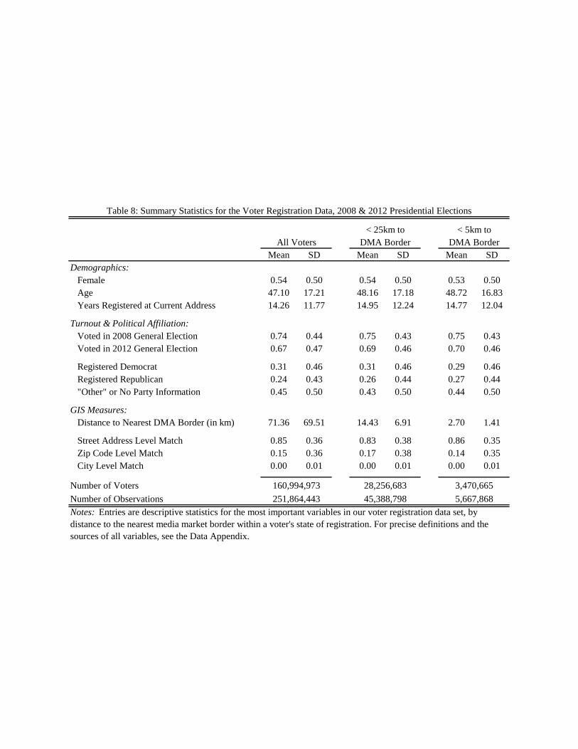
Mean SD Mean SD Mean SD

Demographics:

Female 0.54 0.50 0.54 0.50 0.53 0.50

Age 47.10 17.21 48.16 17.18 48.72 16.83

Years Registered at Current Address 14.26 11.77 14.95 12.24 14.77 12.04

Turnout & Political Affiliation:

Voted in 2008 General Election 0.74 0.44 0.75 0.43 0.75 0.43

Voted in 2012 General Election 0.67 0.47 0.69 0.46 0.70 0.46

Registered Democrat 0.31 0.46 0.31 0.46 0.29 0.46

Registered Republican 0.24 0.43 0.26 0.44 0.27 0.44

"Other" or No Party Information 0.45 0.50 0.43 0.50 0.44 0.50

GIS Measures:

Distance to Nearest DMA Border (in km) 71.36 69.51 14.43 6.91 2.70 1.41

Street Address Level Match 0.85 0.36 0.83 0.38 0.86 0.35

Zip Code Level Match 0.15 0.36 0.17 0.38 0.14 0.35

City Level Match 0.00 0.01 0.00 0.01 0.00 0.01

Number of Voters

Number of Observations

Notes: Entries are descriptive statistics for the most important variables in our voter registration data set, by

distance to the nearest media market border within a voter's state of registration. For precise definitions and the

sources of all variables, see the Data Appendix.

Table 8: Summary Statistics for the Voter Registration Data, 2008 & 2012 Presidential Elections

All Voters DMA BorderDMA Border

251,864,443 45,388,798 5,667,868

< 25km to < 5km to

160,994,973 28,256,683 3,470,665

A. Partisan Difference in Turnout across DMA Borders

Local Polynomial 500 1,000 5,000 10-fold C-V

Linear 0.011 0.015* 0.016** 0.018**

(0.009) (0.007) (0.003) (0.004)

Quadratic 0.014 0.009 0.019** 0.019**

(0.010) (0.009) (0.005) (0.006)

Cubic 0.023 0.012 0.018** 0.018**

(0.012) (0.010) (0.007) (0.007)

Quartic 0.017 0.013 0.019** 0.020**

(0.012) (0.011) (0.007) (0.008)

Number of Observations 214,950 461,645 3,198,904 --

B. Wald Estimator

Local Polynomial 500 1,000 5,000 10-fold C-V

Linear 0.005 0.006 0.006** 0.007**

(0.004) (0.003) (0.002) (0.002)

Quadratic 0.007 0.004 0.008** 0.008*

(0.005) (0.004) (0.003) (0.003)

Cubic 0.012 0.006 0.008* 0.008*

(0.006) (0.005) (0.004) (0.003)

Quartic 0.009 0.007 0.009* 0.009*

(0.006) (0.005) (0.004) (0.004)

Number of Observations 214,950 461,645 3,198,904 --

Table 9: RD Estimates of the Effect of Partisan Differences in Political Advertising on Partisan Differences

in Turnout, 2008 & 2012 Presidential Elections

Bandwidth (in meters)

Notes: Entries in the upper panel are estimates of the discontinuity in the partisan difference in turnout across

media market borders, i.e., τ in equation (4). Larger values indicate an increase in turnout of registered

Democrats relative to registered Republicans. The lower panel displays Wald estimates of the effect of

partisan differences in political advertising on partisan differences in turnout (cf. equation (3)). All Wald

estimates have been scaled so that the coefficients refer to the impact of 10 impressions per capita. As

explained in the main text, the running variable is voters' distance to the nearest within-state media market

border. All estimates are based on local polynomial regressions using a rectangular kernel. The order of the

local polynomial is given on the left of each row, while the respective bandwidth is indicated at the top of

each column. The rightmost column uses 10-fold cross-validation for bandwidth selection, with the holdout

sample consisting of observations that lie within 3km of a media market border. Following Imbens and

Lemieux (2008), we use the optimally chosen bandwidth for the outcome equation for the Wald estimator.

To account for unobserved spatial heterogeneity, every specification includes party-specific fixed effects for

individual border segments of up to 10km length. Heteroskedasticity robust standard errors are clustered by

media market border and reported in parentheses. ** and * denote statistical significance at the 1%- and 5%-

levels, respectively.

Bandwidth (in meters)

A. Wald Estimates for Unaffiliated Voters

Local Polynomial 500 1,000 5,000 10-fold C-V

Linear -0.001 -0.001 -0.001 -0.001

(0.001) (0.001) (0.001) (0.001)

Quadratic -0.001 -0.003* -0.001 0.000

(0.001) (0.001) (0.001) (0.001)

Cubic -0.001 -0.002 -0.001 -0.001

(0.002) (0.001) (0.001) (0.001)

Quartic -0.001 -0.001 -0.001 -0.002

(0.002) (0.001) (0.001) (0.001)

Number of Observations 190,883 383,419 2,468,964 --

B. Wald Estimates for All Voters

Local Polynomial 500 1,000 5,000 10-fold C-V

Linear -0.001 -0.001 -0.001 -0.001

(0.001) (0.001) (0.001) (0.001)

Quadratic -0.001 -0.002* -0.001 0.000

(0.001) (0.001) (0.001) (0.001)

Cubic -0.001 -0.001 0.000 0.000

(0.001) (0.001) (0.001) (0.001)

Quartic -0.001 -0.001 -0.001 -0.001

(0.001) (0.001) (0.001) (0.001)

Number of Observations 405,833 845,064 5,667,868 --

Table 10: Total Political Advertising and Turnout, 2008 & 2012 Presidential Elections

Bandwidth (in meters)

Bandwidth (in meters)

Notes: Entries in the upper panel are Wald estimates of the impact of total presidential advertising on turnout

among voters who are not affiliated with either of the two major parties. The lower panel displays Wald

estimates of the impact of total presidential advertising on all registered voters. All estimates have been

scaled so that the coefficients refer to the impact of 10 impressions per capita. As explained in the text, the

running variable is voters' distance to the nearest within-state media market border. All estimates are based on

local polynomial regressions using a rectangular kernel. The order of the local polynomial is given on the left

of each row, while the respective bandwidth is indicated at the top of each column. The rightmost column

uses 10-fold cross-validation for bandwidth selection, with the holdout sample consisting of observations that

lie within 3km of a media market border. Following Imbens and Lemieux (2008), we use the optimally

chosen bandwidth for the outcome equation of the Wald estimator. To account for unobserved spatial

heterogeneity, every specification includes fixed effects for individual border segments of up to 10km length.

Heteroskedasticity robust standard errors are clustered by media market border and reported in parentheses.

** and * denote statistical significance at the 1%- and 5%-levels, respectively.