Policy Options to Reduce Unemployment: TRYM Simulations

Policy Options to Reduce Unemployment: TRYM Simulations*

Lei Lei Song†, John Freebairn‡ and Don Harding† †Melbourne Institute of Applied Economic and Social Research, The University of Melbourne

‡Department of Economics, The University of Melbourne

Melbourne Institute Working Paper No. 19/01

ISSN 1328-4991 ISBN 0 7340 1523 2

December 2001

* This paper is the result of work being undertaken as part of a collaborative research program entitled 'Unemployment: Economic Analysis and Policy Modelling'. The project is generously

supported by the Australian Research Council and the following collaborative partners: Commonwealth Department of Family and Community Services, Commonwealth Department of Employment, Workplace Relations and Small Business and the Productivity Commission. The views expressed in this paper represent those of the authors and are not necessarily the views of the collaborative partners. The authors wish to thank the Economic Group in Commonwealth Treasury and Peter Downes for helpful discussions. Thanks also due to Peter Dawkins, Peter Dixon and participants at the Melbourne Institute of Applied Economic and Social Research

Conference on Unemployment August 2001 for useful comments.

Melbourne Institute of Applied Economic and Social Research

The University of Melbourne Victoria 3010 Australia

Telephone (03) 8344 5330 Fax (03) 8344 5630

Email [email protected] WWW Address http://www.melbourneinstitute.com

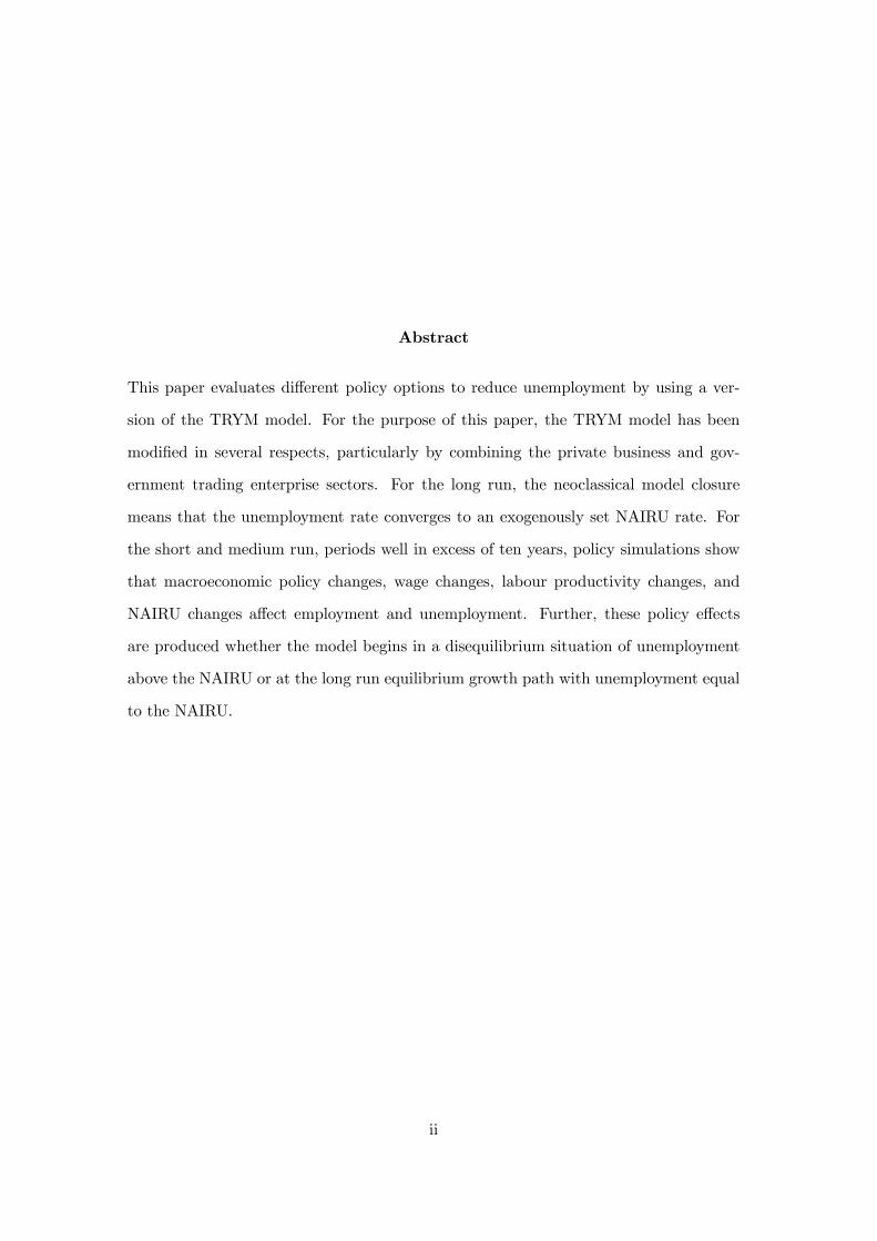
Abstract

This paper evaluates different policy options to reduce unemployment by using a ver-

sion of the TRYM model. For the purpose of this paper, the TRYM model has been

modified in several respects, particularly by combining the private business and gov-

ernment trading enterprise sectors. For the long run, the neoclassical model closure

means that the unemployment rate converges to an exogenously set NAIRU rate. For

the short and medium run, periods well in excess of ten years, policy simulations show

that macroeconomic policy changes, wage changes, labour productivity changes, and

NAIRU changes affect employment and unemployment. Further, these policy effects

are produced whether the model begins in a disequilibrium situation of unemployment

above the NAIRU or at the long run equilibrium growth path with unemployment equal

to the NAIRU.

ii

1 Introduction

This paper is part of the ARC-funded Unemployment SPIRT Research Project. The

broad objective of the Project is to evaluate the pros and cons of different policy

options to reduce unemployment. The purpose of the paper is to use the Treasury

Macroeconomic Model (TRYM ) to simulate various policy changes and to assess the

effects of these changes on employment and unemployment. Specific policy options

investigated with a version of TRYM in this paper are:

• faster economic growth promoted by stimulatory macroeconomic policies:

— monetary policy specified as a period of lower short-term interest rates

— fiscal policy specified as

∗ a period of higher government consumption expenditure, or

∗ a period of higher government investment expenditure, or

∗ a period of lower labour income taxation rates;

• a period of lower average wages than otherwise;

• an increase in labour productivity associated with, for example, better educationand training, or with microeconomic reform;

• a sustained reduction in the non-accelerating-inflation rate of unemployment (NAIRU )associated with, for example, changes to the income tax and social security systems

or the industrial relations system.

The authors have modified the TRYM model for the purpose of the Project. Most

of the research focuses on the employment outcomes, with unemployment being a close

mirror because of low labour supply response elasticities. Only general comments on

the comparative effects of the policy options on other performance measures, such as

GDP, inflation, and the balance of payments, produced in the simulations are discussed

in this paper.

The structure of the paper is as follows. Section 2 provides some overview comments

on the strengths and weaknesses of using a macroeconometric model in general, and

1

TRYM in particular, to evaluate the comparative properties of different policy options

to reduce unemployment. Section 3 describes TRYM in more detail, and in particular

it discusses the modifications to the model which have been made for this study. The

structure and some properties of the model are also discussed. Section 4 outlines policy

options used in the simulations.

Because of the importance of the base case scenario, specifically whether the sim-

ulations start with an economy close to a full employment equilibrium or with high

unemployment, policy simulations are evaluated in sections 5 and 6 for a base case

with unemployment equal to the NAIRU and with unemployment above the NAIRU,

respectively. Sections 5 and 6 note and comment on the underlying model assumptions

and parameters driving the results, and they summarise, compare and contrast TRYM

model estimates of the effects of the different policy options to reduce unemployment.

A final section provides an overall assessment, tentative conclusions, and suggestions for

further work.

2 Macroeconometric modelling

A macroeconometric model, such as TRYM, has a number of advantages and disad-

vantages for policy analysis relative to, say, a qualitative and informal model analysis,

partial equilibrium models and time series models. Here TRYM is used to illustrate

some of these advantages and disadvantages.

The TRYMmodel captures most of the important direct and indirect, or feed forward

and feedback, linkages in the economy. For example, changes in wages affect business

hiring and investment decisions, they affect household incomes and consumption expen-

ditures, they affect pricing decisions, and the model captures interrelationships between

prices and quantities. In TRYM, monetary and fiscal policy settings can be made exoge-

nous or set as endogenous policy reaction functions. These and other general equilibrium

interactions are left out of partial equilibrium models, often they are implicit or ignored

in qualitative analyses, and they are treated in a highly aggregated way in time series

models.

Macroeconometric models, like any formal model, require the investigator to make

2

explicit assumptions about functions and parameters. This has the advantages of fo-

cussing the analyst’s mind, of providing a way of explaining the underlying logic and

transmission processes from policy change to simulated policy responses, and for focus-

ing the debate on key areas of uncertainty and their effects.

The general analytical structure of TRYM, however, imposes a priori a number of

important constraints which in turn partly predetermine the simulated effects of different

policy options to reduce unemployment. TRYM has a long run neoclassical equilibrium

closure. Pre-specified growth rates for labour augmenting technical change and work-

force growth, and an essentially exogenous NAIRU, together with the requirements of

model consistency and identities, determine the long run equilibrium growth rate of

GDP and its components. In the long run monetary policy has no real effects, and

the monetary policy rule determines inflation and nominal wage growth rates. Impor-

tantly, for analysis of policies to reduce unemployment, the long run structure of TRYM,

and assuming a convergent system, means that all policy alternatives have no long run

employment or unemployment effects.

However, in the short and medium term, a period which exceeds ten years, TRYM

simulations of aggregate prices and quantities can and do deviate from the long run equi-

librium growth path. Short run dynamics, usually formulated as error correction models

and estimated using historical time series data, arise from sticky wages and prices, from

adjustment costs and lags, and from private sector expectations and government policy

reaction functions which are in part driven by backward looking adjustments rather

than entirely by rational long run model consistent outcomes. Because of these short

run dynamics, macroeconomic expansion policies, wage interventions, and productivity

changes will have short and medium term effects on employment and unemployment in

TRYM simulations.

Short run dynamics in TRYM simulations show a clear pattern of cycles and oscil-

lations towards the long run equilibrium path. These cycles and oscillations are partly

driven by slow stock adjustments, which result in under- and over-shooting of endoge-

nous flow variables. Backward looking policy responses, and private sector expectations,

are other important model structural characteristics contributing to the cyclical pattern.

3

The model assumptions and estimated parameters for short run adjustments in

TRYM represent a mixture of a priori specification and data estimation. As will be

argued, they affect the simulated effects of policy options, and there can be legitimate

debate as to their appropriateness as a simplified model of the Australian macroeconomy.

Results of TRYM simulations of fiscal and monetary policy stimuli are conditioned by

lagged adjustments built into the model and by crowding out effects. The combination

of backward looking expectations (though forward looking in financial markets) and

sluggish responses of real quantities and some prices can generate cyclical responses and

phases of undershooting and overshooting of responses to changes in policy and other

exogenous variables. Crowding out effects arising from changes in government borrowing

requirements affect interest rates, which in turn have impacts on business investment

and international capital inflows, with the latter affecting the exchange rate and then

net exports. Increases in domestic absorption push up domestic prices which in turn

change real labour costs and international competitiveness.

Labour market effects of the different policy scenarios, directly in the case of wage

cuts and labour productivity improvements and indirectly via macroeconomic policy

expansion effects on inflation and real wages, in TRYM clearly are influenced by the

way in which the labour market is modelled. Labour demand and investment demand in

the business sector come from a profit maximising neoclassical model, with an estimated

long run labour demand elasticity of -0.72 reflecting substitutability of labour and capital

in production. A Phillips curve, or wage offer curve, adjusts wage rates in response to

unemployment deviations from the NAIRU rate. Real wages have no effects on labour

supply, but employment does have an encouraged worker effect in both the short and

long run.

Interesting and important characteristics of TRYM are its inclusion of policy reaction

functions for fiscal and monetary policy. In practice, Treasury modellers have exper-

imented with alternative policy reaction functions, and the default reaction functions

used in this paper are only a particular example chosen from a number of possible func-

tions. Before turning to the discussion of simulation results, the next section discusses

the details of TRYM and of modifications made for the purpose of this project.

4

3 The TRYM model

The TRYM model is a small scale macroeconometric model of the Australian economy

for “macroeconomic forecasting, policy analysis and sensitivity analysis”.1 It has 122

equations, and among them 26 equations are estimated over the period since the late

1960s. There are three financial market identities, and two policy reaction functions.

Treasury modellers describe “the model as broadly new Keynesian in its dynamic struc-

ture but with an equilibrating long run” (Downes and Bernie, 1999, P.i). Economic

activity in TRYM is demand determined in the short run but supply determined in the

long run.

3.1 The host model

The host model used in the paper is the June 2000 release of the TRYM model. This

release, representing the TRYM model in recent years, is different in some aspects from

the public release in 1996. Detailed discussion of the properties of the June 2000 release

(and previous releases) can be found in Harding and Song (2001).

3.1.1 Model structure

The TRYM model is an aggregate, quarterly macroeconometric model. A long run

neoclassical balanced growth path with short run error correction adjustments is imposed

in the model.

In the long run, the real economy will grow at a constant rate equal to the underlying

growth of labour productivity represented as Harrod neutral technical change, plus pop-

ulation growth. All prices in the long run will grow at the rate of inflation exogenously

determined by the growth rate of money set by the monetary authority.

In the short run, however, there exists price stickiness. Product prices are assumed

to adjust slowly toward their equilibrium levels which are derived from a production

function. A homogeneity constraint is imposed so that changes in prices will eventually

be fully reflected in changes in nominal wages.

The TRYM model assumes that the agents in the goods and labour markets are

1The details of the TRYM model are described in Commonwealth Treasury (1996a; 1996b).

5

https://www.researchgate.net/publication/255650452_The_Macroeconomics_of_Unemployment_in_the_Treasury_Macroeconomic_TRYM_Model?el=1_x_8&enrichId=rgreq-8289fdf7b0db0a28624960f29daea21a-XXX&enrichSource=Y292ZXJQYWdlOzUxMDMzNjU7QVM6OTg3NjE2OTUwMzk0OThAMTQwMDU1ODAzMTc5OA==

backward looking, whereas those in the financial markets are assumed to have “quasi-

rational” (or “quasi model consistent”) expectations (Commonwealth Treasury, 1996b,

p.2.7). The agents in the financial markets are assumed to know enough about the

fundamental structure of the economy to form judgements about the equilibrium price

level and the equilibrium exchange rate.

There are three decision units: private business, household, and public; and three

markets: goods (domestic and international), labour and financial.

In the private business sector, a representative competitive or price-taking firm is

assumed to maximise profits. Production of goods and services uses capital and labour

as inputs into a CES production process. Derived decisions determine labour demand,

investment and prices. In the long run, returns to labour and capital are equal to their

marginal products and prices are a function of nominal unit labour costs. Tobin’s Q,

together with capacity utilisation, is a major determinant of business investment in the

short run. In the long run, business investment equates the expected rate of return

on the capital stock (which is the marginal product of capital) to the required rate of

return.

The household sector decides consumption, labour supply and dwelling investment.

Consumption is a function of after-tax labour income and private wealth. Once house-

holds have determined their total level of aggregate consumption, they choose between

the consumption of rental services and non-rental consumption according to relative

prices. The dwellings sector produces rental services from dwelling capital. Similar to

the private business sector, dwelling investment is determined by its Q ratio.

The public sector distinguishes between government enterprises and general govern-

ment. Government enterprises are assumed to have the same underlying production

process as private firms. The general government sub-sector has functions for expendi-

ture, revenue and the public sector borrowing requirement. While expenditure is usually

set exogenously and indirect tax rates are also exogenous, indirect tax revenue fluctuates

with changes in the tax base. The income tax rates respond to movements in public

sector debt, and they are determined endogenously such that the public debt to GDP

ratio returns to an exogenous target value in the long run.

6

The goods market, domestic or international, balances expenditure and output deci-

sions. The price block determines relative prices for the four major expenditure aggre-

gates: non-rental consumption, government market demand, business investment and

investment in dwellings. Exports are separated into commodities and non-commodities.

It is assumed that the world demand for Australian commodity exports is perfectly

elastic, hence commodity exports are determined by supply side factors. In contrast,

non-commodity exports are assumed to face a downward sloping world demand curve

and to have a perfectly elastic supply curve. That is, local non-commodity exports are

determined by world demand given the domestic price of non-commodities.

The basic labour market framework in TRYM bears many similarities with the sys-

tem outlined in Layard, Nickell, and Jackman (1991, Chapter 8).2 Labour supply is

a function of the employment rate (representing an encouraged worker effect) and an

exogenous trend. Labour demand by the private sector depends on output and real

producer wages. A Beveridge curve relates unemployment to vacancies and represents

matching efficiency in the labour market. A long run exogenous NAIRU means that

labour demand ultimately depends on labour supply in equilibrium. A short run Phillips

curve (or wage offer curve) relates changes in the expected real consumer wage to the

unemployment rate and to changes in the unemployment rate, among other things.

The financial market is represented by three financial identities and an inverted

money demand function. The inverted money demand function determines the full

information short-term interest rate as a function of gross national expenditure and

exogenous money supply that is based on a money supply rule. Nominal money supply

is assumed to grow at a constant rate in simulations, equal to the equilibrium real supply

growth rate plus an exogenous long run inflation rate target. The actual short-term

interest rate is decided by a monetary policy reaction function, in terms of the degree

of accommodation for monetary policy (or the extent of interest rate smoothing).

The bond yield identity relates the expected real long-term interest rate, which is

the rate for investment decisions, to the expected real short-term interest rate. The

inflationary expectations identity forms agents’ inflationary expectations from the ten-

2The detailed discussions of the labour market in TRYM can be found in Downes and Bernie (1999)and Thomson (2000).

7

year-ahead equilibrium price level (obtained from simulations using the steady state

version of TRYM). The current exchange rate is determined by uncovered interest rate

parity, which relates the expected deviation of the exchange rate from its long run

equilibrium level (ten years ahead) to the interest rate differential between Australia

and the rest of the world. The future equilibrium exchange rate is derived from the

steady state version of the model, which achieves internal balance and a stable ratio of

net external liabilities to GDP.

The financial markets are said to be “quasi-rational”, that is, “agents in the financial

markets are assumed to have a mixture of forward looking and adaptive behaviour.”

Rather than solving these expectations to be consistent with the dynamic path taken by

the model, the values of the expectation variables, obtained from a corresponding steady

state simulation, act as forward looking expectations in solving short run dynamics of

endogenous variables.

The default fiscal and monetary policy reaction mechanisms are not forward looking

in TRYM. The labour income tax rate and the short-term interest rate react to current

or previous economic conditions. This implies that following a shock, the model adjusts

slowly towards a new equilibrium. The short run partial adjustment in prices and wages

and non-forward-looking policy reactions make adjustments to shocks sluggish and they

help to generate cyclical responses to changes in policies or other exogenous shocks.

3.1.2 Estimation and model solution

Most estimated equations in TRYM are specified in an error correction model (ECM)

format and the rest use a partial adjustment model or other equilibrating mechanisms.

While ECMs imply a cointegration relationship among the variables in the equation,

the TRYM documentation does not report cointegration test results. The use of ECMs

means that the short and long run properties of an equation are clearly distinguished.

The long run (or the equilibrium) part is often guided and restricted by economic the-

ory. The long run parts of the estimated equations, along with identities and policy

reaction functions, comprise the steady state version of the model. The full version

of the model incorporates short run behaviour and adjustment towards the long run

8

equilibrium growth path.

The steady state version of the model is first solved in the projection period to

derive the long run equilibrium growth path for the model. The equilibrium path of

the three expectation variables then are used as exogenous variables in the full version

of the model, which is solved in the projection period to obtain short run dynamics of

the endogenous variables. The solution is not model consistent, in the sense that the

dynamic path of the expectation variables is different from their equilibrium paths. The

use of two versions of the model enables a modeller to clearly distinguish short run and

long run effects of a policy change.

3.2 Modifications

The production function of the private business sector is the centrepiece of TRYM.

Investment demand, labour demand and price setting for the sector are all derived from

the production function. The estimated parameters of the production function from

the private business sector are also used for the government trading enterprise (GTE)

sector. Simulation properties of the model are heavily influenced by the parameters of

this production function.

Harding and Song (2001) identify that the estimated parameters of the host model

(June 2000 release) yield an equilibrium capital (quarterly) output ratio of 7.8 for the

private sector, well above the current value of 4.6 in the first half of 2000. The estimated

Q ratio, which is a key variable for the determination of investment demand, is about

1.3 on average in the last two decades, always greater than the equilibrium value of one.

Although the capital output ratio in the GTE sector is much higher (about 20) than that

in the private sector, the same set of parameters are used for the GTE sector. Moreover,

the host model might not fully adjust for privatisation-induced capital movements from

the GTE sector to the private sector in the 1990s.

The question of stability of TRYM, discussed in Harding and Song (2001), also needs

to be addressed. Persistent oscillations in model dynamic simulations are not desirable

for policy analysis. Though it is believed to be “quasi-model-consistent”, the model is

not solved consistently, in the sense that forward looking variables are not consistent

9

with the dynamic model solutions. In addition, it appears that some estimated equations

fail key diagnostic tests and do not fit the historical data well.

For the above reasons, the host model has been modified to obtain different, and in

our view more reasonable, estimates of the production function and a more desirable

base case scenario run for policy experiment simulations. The major modifications are

outlined as follows:

1. Production functions

The private business and GTE sectors are combined together and only one pro-

duction function is estimated. Subsequently, the GTE sector no long exists in the

modified model. All the variables of the GTE sector are merged into the corre-

sponding variables in the private business sector. Three equations derived from

the production function, labour demand, investment demand and price-setting,

are re-specified and re-estimated. Newly estimated parameters of the production

function such as the productivity parameter are used in other equations.

2. Long-term interest rates

The host model has a short-term (90 day bill) and a long-term (10-year-bond) in-

terest rates. Experiments show that persistent oscillations in dynamic simulations

is also due to the sluggish response of the long-term interest rate to changes in the

short-term interest rate, which in turn significantly slow down the adjustments in

real activities. The long-term interest rate has been deleted in the modified model.

Deletion of the long-term interest rate brings about much quicker adjustments and

cycles in dynamic simulations dampens over time.

3. Uncovered interest rate parity

Rather than ten years in the host model, uncovered interest rate parity is assumed

to hold in a quarter. Experiments show that assuming interest rate parity over

one year has negligible effects on simulation results.

4. Model solution

Similar to the host model, the modified model has two separate sets of equations;

one is for the steady state and the other one is the full version to include short

10

run dynamics. The steady state version of the model is used to obtain the starting

values of the expectation variables and it also provides the terminal conditions

for the three expectation variables for a dynamic simulation. The full version of

the modified model is solved by using the Fair-Taylor (1983) extended path proce-

dure for rational expectations models, generating the dynamic path of endogenous

variables.3 The host TRYM model does not apply the Fair-Taylor procedure.

5. Other modifications

Since the structure of the model is changed, some data series have been re-

constructed, such as the price of business output, the price of non-commodities and

the depreciation rate of business sector capital stock. Apart from the equations de-

rived from the production function, several other equations are re-specified, such as

wage-setting, price of investment, price of imports and hours worked. Some minor

mistakes in the host model have also been corrected. After theses modifications,

the model has been re-estimated.

3.3 Testing the modified model

Treasury modellers have designed two tests of internal consistency for the TRYM model.

The steady state bias test is to test the consistency between the steady state version of

equations and the full version of equations. This is done by simulating the full version

from a point of time on the steady state path. The resulting dynamic path of every

endogenous variable should not be different from its steady state path. The modified

model passes the steady state bias test.

The counter-factual simulation test is to evaluate how well the model tracks history.

This test is made conditioned on the actual path of the interest rates, the exchange rate,

inflationary expectations and nominal wages, and all the estimated equation residuals.

These variables are endogenous in the model when a counter-factual simulation is con-

ducted. Although the money demand function is estimated by using an error correction

equation, only the long run part of the error correction equation is used in the TRYM

3Solving the model by the Fair-Taylor extended path procedure is very time consuming. A dynamicsimulation for 50 years normally takes about one hour to run on an Unix machine (DEC Alpha).

11

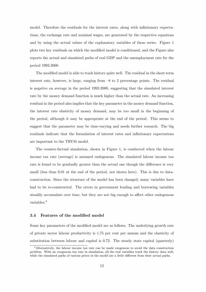
model. Therefore the residuals for the interest rates, along with inflationary expecta-

tions, the exchange rate and nominal wages, are generated by the respective equations

and by using the actual values of the explanatory variables of these series. Figure 1

plots two key residuals on which the modified model is conditioned, and the Figure also

reports the actual and simulated paths of real GDP and the unemployment rate for the

period 1992-2000.

The modified model is able to track history quite well. The residual in the short-term

interest rate, however, is large, ranging from —8 to 2 percentage points. The residual

is negative on average in the period 1992-2000, suggesting that the simulated interest

rate by the money demand function is much higher than the actual rate. An increasing

residual in the period also implies that the key parameter in the money demand function,

the interest rate elasticity of money demand, may be too small in the beginning of

the period, although it may be appropriate at the end of the period. This seems to

suggest that the parameter may be time-varying and needs further research. The big

residuals indicate that the formulation of interest rates and inflationary expectations

are important to the TRYM model.

The counter-factual simulation, shown in Figure 1, is conducted when the labour

income tax rate (average) is assumed endogenous. The simulated labour income tax

rate is found to be gradually greater than the actual one though the difference is very

small (less than 0.01 at the end of the period, not shown here). This is due to data-

construction. Since the structure of the model has been changed, many variables have

had to be re-constructed. The errors in government lending and borrowing variables

steadily accumulate over time, but they are not big enough to affect other endogenous

variables.4

3.4 Features of the modified model

Some key parameters of the modified model are as follows. The underlying growth rate

of private sector labour productivity is 1.75 per cent per annum and the elasticity of

substitution between labour and capital is 0.72. The steady state capital (quarterly)

4Alternatively, the labour income tax rate can be made exogenous to avoid the data constructionproblem. With an exogenous tax rate in simulation, all the real variables track the history data well,while the simulated paths of various prices in the model are a little different from their actual paths.

12

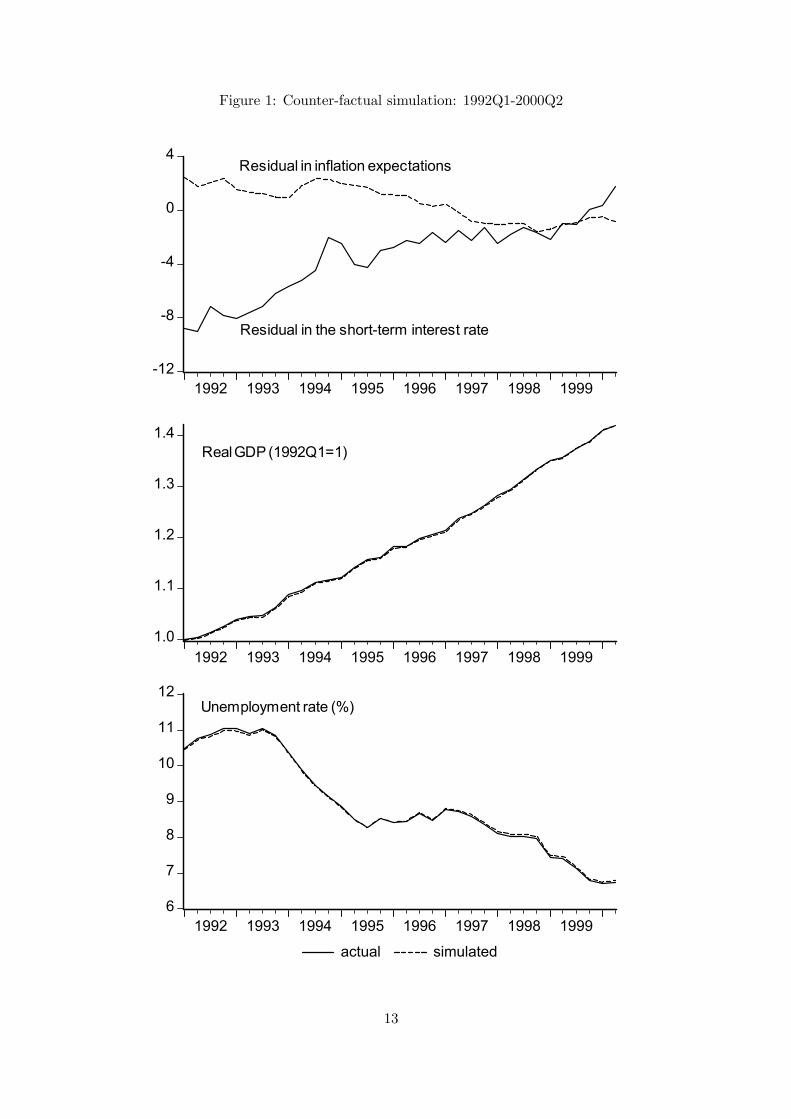
Figure 1: Counter-factual simulation: 1992Q1-2000Q2

-12

-8

-4

0

4

1992 1993 1994 1995 1996 1997 1998 1999

Residual in inflation expectations

Residual in the short-term interest rate

1.0

1.1

1.2

1.3

1.4

1992 1993 1994 1995 1996 1997 1998 1999

Real GDP (1992Q1=1)

6

7

8

9

10

11

12

1992 1993 1994 1995 1996 1997 1998 1999

actual simulated

Unemployment rate (%)

13

output ratio is about 7.1 if the world interest rate is set at 6 per cent per year and the risk

premium for investing in Australia is 1 per cent. Given that the actual capital output

ratio has been about 6.3 in the last two decades, the new estimate is more reasonable

than the host model. The newly estimated Q ratio is 1.08 on average for the last two

decades.

The estimated NAIRU is 6.02 per cent, with a standard error of 0.66 per cent, a

little higher than the host model. A permanent reduction in the level of the NAIRU

of 1 percentage point would lead to a temporary reduction in nominal wage growth of

about 0.19 of a percentage point per quarter, other things being equal. In other words,

if the unemployment rate was 1 percentage point higher than the level of the NAIRU,

this would result in wage deflation of about three quarters of a percentage point per

year. This is, however, a temporary effect as nominal wage growth would return to the

level of price inflation once the unemployment rate had fallen to the new NAIRU. In

the long run, the unemployment rate equals the NAIRU.

The interest rate semi-elasticity of money demand is about 2, suggesting that in-

creasing short term interest rates by 1 percentage point would decrease the demand for

money by around 2 per cent in the long run. Any disequilibrium between the actual

and desired price of non-commodities is eliminated very slowly, by around 4 per cent

each quarter.

The fiscal policy reaction function is assumed to be

∆rtnt = a1 × (debtt − debtt) + a2 × {(debtt − debtt)− (debtt−1 − debtt−1)} (1)

where rtn is the rate of tax on labour income, debt is the ratio of government debt to

nominal GDP and debt is the target level of government debt to GDP. Following the

June 2000 release of TRYM, the target level of the debt to GDP ratio is set at the level

of the second quarter of 2000, which is 1.32663. The default values of a1 and a2 are

0.00233 and 0.04, respectively. The parameter values imply a slow response of fiscal

policy to changes in economic conditions. The following equation determines the full

14

information short-term interest rate

RI90X =1

c1

½− ln

µM1

GNEZ

¶− c0

¾(2)

where RI90X is the so-called full information short term interest rate in TRYM, which

relates the short-term interest rate to both changes in the money supply rule and fluctu-

ations in demand. GNEZ is nominal gross national expenditure. In simulations, money

supply (M1 ) grows at a constant rate equal to the underlying growth rate of real supply

plus an exogenous inflation target.5 The default monetary policy reaction function sets

the short-term interest rate equal to the full information short-term rate.

In the rest of the paper, all simulations (except counter factual simulations) assume

that in equilibrium, the world interest rate is 6 per cent, the risk premium is 1 per cent,

the inflation target set by the domestic and foreign monetary authorities is 2.5 per cent

and population growth is 0.78 per cent per annum. The foreign variables used in the

model, such as real GDP, prices and population growth, are extrapolated by using the

respective growth rates of Australia over the projection period.

3.4.1 Dynamic adjustment towards steady state

Given the assumptions for exogenous variables, the model can be simulated dynamically

over a projection period starting in the quarter immediately after the historical data ends

(i.e., the third quarter of 2000), to compare the results of that simulation with the steady

state path. The steady state path is derived from the steady state version of the model,

which excludes the short run components of the TRYM behavioural equations. The

dynamic simulation is conducted on the assumption that all the exogenous variables

are in long run equilibrium starting at the third quarter of 2000. Figure 2 plots the

percentage deviations of three endogenous variables from the steady state path for the

period from the March quarter of 2000 to the June quarter of 2056.6

The graph clearly shows dampened cycles towards the steady state path. While

there are several cycles, the economy converges to the steady state growth path. The

5M1 is defined in TRYM as “currency in the hands of the non-bank private sector plus non-interestbearing current deposits of all banks plus a fixed proportion of interest bearing current accounts of allbanks” (Commonwealth Treasury, 1996a, p.6.2).

6The actual values of the variables are used for the first two quarters in the graph.

15

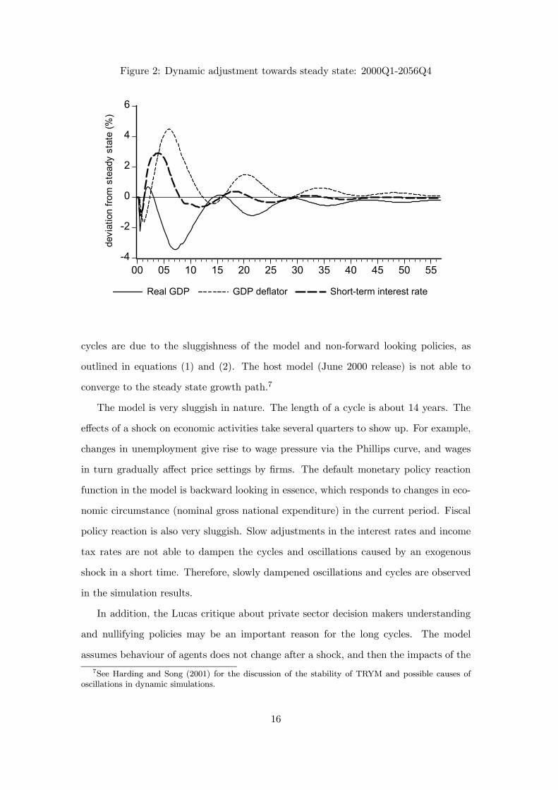
Figure 2: Dynamic adjustment towards steady state: 2000Q1-2056Q4

-4

-2

0

2

4

6

00 05 10 15 20 25 30 35 40 45 50 55

Real GDP GDP deflator Short-term interest rate

devi

atio

n fro

m s

tead

y st

ate

(%)

cycles are due to the sluggishness of the model and non-forward looking policies, as

outlined in equations (1) and (2). The host model (June 2000 release) is not able to

converge to the steady state growth path.7

The model is very sluggish in nature. The length of a cycle is about 14 years. The

effects of a shock on economic activities take several quarters to show up. For example,

changes in unemployment give rise to wage pressure via the Phillips curve, and wages

in turn gradually affect price settings by firms. The default monetary policy reaction

function in the model is backward looking in essence, which responds to changes in eco-

nomic circumstance (nominal gross national expenditure) in the current period. Fiscal

policy reaction is also very sluggish. Slow adjustments in the interest rates and income

tax rates are not able to dampen the cycles and oscillations caused by an exogenous

shock in a short time. Therefore, slowly dampened oscillations and cycles are observed

in the simulation results.

In addition, the Lucas critique about private sector decision makers understanding

and nullifying policies may be an important reason for the long cycles. The model

assumes behaviour of agents does not change after a shock, and then the impacts of the

7See Harding and Song (2001) for the discussion of the stability of TRYM and possible causes ofoscillations in dynamic simulations.

16

shock on the economy gradually factor in.

Treasury modellers have already discarded the default policy reaction functions in

policy analysis, in particular the monetary policy reaction function. Instead, they design

an optimal control algorithm for the short-term interest rate to minimise a loss function

based on inflation, the unemployment rate and changes in the interest rate. The loss

function is forward looking. The aim of the optimal control algorithm is to make mon-

etary policy forward-looking and more responsive to changes in economic conditions.

The algorithm may possibly be able to eliminate oscillations and long cycles and yield

smooth paths of endogenous variables. Unfortunately at this early stage, the Economic

Group has not publicly released satisfactory simulation results from the optimal control

algorithm. Therefore it is hard to compare the algorithm with the default monetary

policy reaction. In addition, the algorithm is complicated and difficult to implement.

Apart from using an optimal control algorithm to specify the monetary policy reac-

tion function, the Treasury modellers alternatively suggest specifying appropriate paths

of the interest rate (or money supply) and/or the income tax rate, to reflect have for-

ward looking monetary and fiscal policies. This approach, to some extent, is a “manual”

optimal control procedure. The procedure may be able to eliminate initial under- and

over-shooting of responses to exogenous shocks in a simulation and therefore to dampen

following cycles. The simulation results using this approach in Downes and Bernie (1999)

show that some variables, such as the unemployment rate, smoothly approach the equi-

librium path; however, still some other variables, such as GDP, cycle substantially.

Following this suggestion, a set of simulations based on accommodating macroeco-

nomic policies was also conducted. In this set of simulations, monetary and fiscal policies

are adjusted at the start of the simulation period to accommodate possible changes in

prices and GDP. The rule for accommodating policy is designed to generate a stable

path of prices in the medium to long run. Either money supply or the interest rate is

adjusted to achieve price stability. It has been found that while the path of endogenous

variables changes, the main outcomes do not. Therefore, the paper does not report the

simulation results based on accommodating macroeconomic policies.

Past history for Australia, and all modern economies, is characterised by cyclical

17


economic behaviour. Many explanations and models have been published. Clearly

there has to be debate about whether the key causal mechanisms in TRYM of cyclical

behaviour, namely sluggish adjustment of prices and quantities to shocks, elements of

backward looking expectations by households, firms and government, and stock-flow

interactions, are the most appropriate causes of Australian cyclical behaviour.

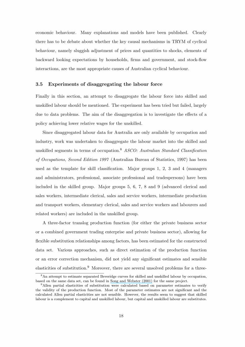
3.5 Experiments of disaggregating the labour force

Finally in this section, an attempt to disaggregate the labour force into skilled and

unskilled labour should be mentioned. The experiment has been tried but failed, largely

due to data problems. The aim of the disaggregation is to investigate the effects of a

policy achieving lower relative wages for the unskilled.

Since disaggregated labour data for Australia are only available by occupation and

industry, work was undertaken to disaggregate the labour market into the skilled and

unskilled segments in terms of occupation.8 ASCO: Australian Standard Classification

of Occupations, Second Edition 1997 (Australian Bureau of Statistics, 1997) has been

used as the template for skill classification. Major groups 1, 2, 3 and 4 (managers

and administrators, professional, associate professional and tradespersons) have been

included in the skilled group. Major groups 5, 6, 7, 8 and 9 (advanced clerical and

sales workers, intermediate clerical, sales and service workers, intermediate production

and transport workers, elementary clerical, sales and service workers and labourers and

related workers) are included in the unskilled group.

A three-factor translog production function (for either the private business sector

or a combined government trading enterprise and private business sector), allowing for

flexible substitution relationships among factors, has been estimated for the constructed

data set. Various approaches, such as direct estimation of the production function

or an error correction mechanism, did not yield any significant estimates and sensible

elasticities of substitution.9 Moreover, there are several unsolved problems for a three-

8An attempt to estimate separated Beveridge curves for skilled and unskilled labour by occupation,based on the same data set, can be found in Song and Webster (2001) for the same project.

9Allen partial elasticities of substitution were calculated based on parameter estimates to verifythe validity of the production function. Most of the parameter estimates are not significant and thecalculated Allen partial elasticities are not sensible. However, the results seem to suggest that skilledlabour is a complement to capital and unskilled labour, but capital and unskilled labour are substitutes.

18

https://www.researchgate.net/publication/5103360_How_Segmented_Are_Skilled_and_Unskilled_Labour_Markets_The_Case_of_Beveridge_Curves?el=1_x_8&enrichId=rgreq-8289fdf7b0db0a28624960f29daea21a-XXX&enrichSource=Y292ZXJQYWdlOzUxMDMzNjU7QVM6OTg3NjE2OTUwMzk0OThAMTQwMDU1ODAzMTc5OA==

factor production function in TRYM, such as technology progress and an under-identified

system of equations about the labour market. While the attempt failed, it points to an

important area for future research.

4 Policy options

The combination of (a) exogeneity of long run effects of different policy scenarios on

macroeconomic performance, including unemployment, and (b) the scope for large short

run and medium run deviations from the long run equilibrium path means that it is

necessary to consider the starting point in TRYM simulations. This paper looks at two

options:

• start at the NAIRU rate of unemployment and assess the comparative short runand any cyclical effects of policy options to reduce unemployment; and

• start at an unemployment rate well above the NAIRU and compare and contrastthe paths of the economy to the long run equilibrium in response to different policy

strategies.

Literally, the second one is chosen at 1992 when the unemployment rate of 10.8 per

cent was well above the TRYM model estimated NAIRU of 6.02 per cent. The policy

simulations starting at 1992 are counter factual simulations to assess the would-be effects

on the economy if there had been a policy change.

Specifically, the following policy options are implemented for each starting point:

1. Monetary expansion: the interest rate is cut by 1 percentage point for each of the

next three years (one and half years for the counter-factual policy simulation). In

equilibrium, the short-term interest rate is cut from 7 per cent to 6 per cent in the

current set-up.

2. Increasing government spending (fiscal expansions): government expenditure in-

creased by 3.62 per cent for each of the next three years (one and half years for

the counter-factual policy simulation). This is equivalent to about an increase of

$2 billion in 1999-2000.

19

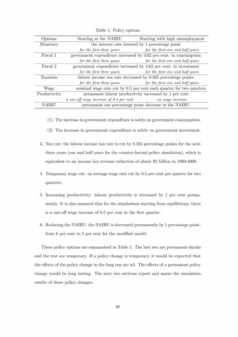
Table 1: Policy options

Options Starting at the NAIRU Starting with high unemployment

Monetary the interest rate lowered by 1 percentage pointfor the first three years for the first one and half years

Fiscal 1 government expenditure increased by 3.62 per cent: in consumptionfor the first three years for the first one and half years

Fiscal 2 government expenditure increased by 3.62 per cent: in investmentfor the first three years for the first one and half years

Taxation labour income tax rate decreased by 0.565 percentage pointsfor the first three years for the first one and half years

Wage nominal wage rate cut by 0.5 per cent each quarter for two quarters

Productivity permanent labour productivity increased by 1 per centa one-off wage increase of 0.5 per cent no wage increase

NAIRU permanent one percentage point decrease in the NAIRU

(1) The increase in government expenditure is solely on government consumption.

(2) The increase in government expenditure is solely on government investment.

3. Tax cut: the labour income tax rate is cut by 0.565 percentage points for the next

three years (one and half years for the counter-factual policy simulation), which is

equivalent to an income tax revenue reduction of about $2 billion in 1999-2000.

4. Temporary wage cut: an average wage rate cut by 0.5 per cent per quarter for two

quarters.

5. Increasing productivity: labour productivity is increased by 1 per cent perma-

nently. It is also assumed that for the simulations starting from equilibrium, there

is a one-off wage increase of 0.5 per cent in the first quarter.

6. Reducing the NAIRU: the NAIRU is decreased permanently by 1 percentage point,

from 6 per cent to 5 per cent for the modified model.

These policy options are summarised in Table 1. The last two are permanent shocks

and the rest are temporary. If a policy change is temporary, it would be expected that

the effects of the policy change in the long run are nil. The effects of a permanent policy

change would be long lasting. The next two sections report and assess the simulation

results of these policy changes.

20

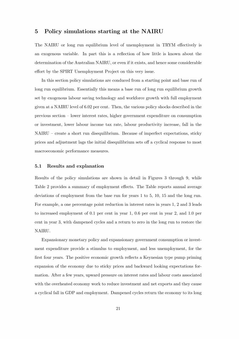
5 Policy simulations starting at the NAIRU

The NAIRU or long run equilibrium level of unemployment in TRYM effectively is

an exogenous variable. In part this is a reflection of how little is known about the

determination of the Australian NAIRU, or even if it exists, and hence some considerable

effort by the SPIRT Unemployment Project on this very issue.

In this section policy simulations are conduced from a starting point and base run of

long run equilibrium. Essentially this means a base run of long run equilibrium growth

set by exogenous labour saving technology and workforce growth with full employment

given at a NAIRU level of 6.02 per cent. Then, the various policy shocks described in the

previous section — lower interest rates, higher government expenditure on consumption

or investment, lower labour income tax rate, labour productivity increase, fall in the

NAIRU — create a short run disequilibrium. Because of imperfect expectations, sticky

prices and adjustment lags the initial disequilibrium sets off a cyclical response to most

macroeconomic performance measures.

5.1 Results and explanation

Results of the policy simulations are shown in detail in Figures 3 through 9, while

Table 2 provides a summary of employment effects. The Table reports annual average

deviations of employment from the base run for years 1 to 5, 10, 15 and the long run.

For example, a one percentage point reduction in interest rates in years 1, 2 and 3 leads

to increased employment of 0.1 per cent in year 1, 0.6 per cent in year 2, and 1.0 per

cent in year 3, with dampened cycles and a return to zero in the long run to restore the

NAIRU.

Expansionary monetary policy and expansionary government consumption or invest-

ment expenditure provide a stimulus to employment, and less unemployment, for the

first four years. The positive economic growth reflects a Keynesian type pump priming

expansion of the economy due to sticky prices and backward looking expectations for-

mation. After a few years, upward pressure on interest rates and labour costs associated

with the overheated economy work to reduce investment and net exports and they cause

a cyclical fall in GDP and employment. Dampened cycles return the economy to its long

21

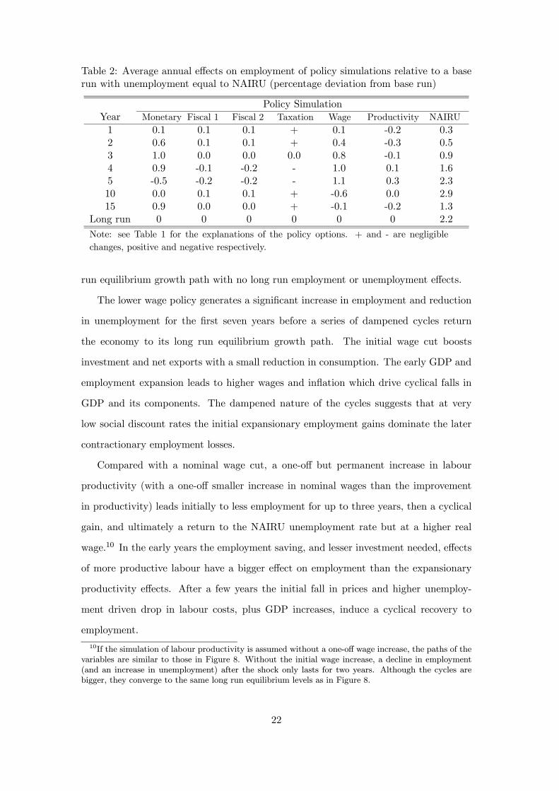
Table 2: Average annual effects on employment of policy simulations relative to a baserun with unemployment equal to NAIRU (percentage deviation from base run)

Policy SimulationYear Monetary Fiscal 1 Fiscal 2 Taxation Wage Productivity NAIRU

1 0.1 0.1 0.1 + 0.1 -0.2 0.32 0.6 0.1 0.1 + 0.4 -0.3 0.53 1.0 0.0 0.0 0.0 0.8 -0.1 0.94 0.9 -0.1 -0.2 - 1.0 0.1 1.65 -0.5 -0.2 -0.2 - 1.1 0.3 2.310 0.0 0.1 0.1 + -0.6 0.0 2.915 0.9 0.0 0.0 + -0.1 -0.2 1.3

Long run 0 0 0 0 0 0 2.2

Note: see Table 1 for the explanations of the policy options. + and - are negligible

changes, positive and negative respectively.

run equilibrium growth path with no long run employment or unemployment effects.

The lower wage policy generates a significant increase in employment and reduction

in unemployment for the first seven years before a series of dampened cycles return

the economy to its long run equilibrium growth path. The initial wage cut boosts

investment and net exports with a small reduction in consumption. The early GDP and

employment expansion leads to higher wages and inflation which drive cyclical falls in

GDP and its components. The dampened nature of the cycles suggests that at very

low social discount rates the initial expansionary employment gains dominate the later

contractionary employment losses.

Compared with a nominal wage cut, a one-off but permanent increase in labour

productivity (with a one-off smaller increase in nominal wages than the improvement

in productivity) leads initially to less employment for up to three years, then a cyclical

gain, and ultimately a return to the NAIRU unemployment rate but at a higher real

wage.10 In the early years the employment saving, and lesser investment needed, effects

of more productive labour have a bigger effect on employment than the expansionary

productivity effects. After a few years the initial fall in prices and higher unemploy-

ment driven drop in labour costs, plus GDP increases, induce a cyclical recovery to

employment.

10If the simulation of labour productivity is assumed without a one-off wage increase, the paths of thevariables are similar to those in Figure 8. Without the initial wage increase, a decline in employment(and an increase in unemployment) after the shock only lasts for two years. Although the cycles arebigger, they converge to the same long run equilibrium levels as in Figure 8.

22

The lower NAIRU policy shock has long run effects of increased employment and

lower unemployment, in contrast to other policies where long run effects are assumed

away. Because of sticky wages and adjustment costs, employment growth is relatively

slow, and these same factors give rise to a series of dampened cycles before converging

to the new long run equilibrium growth path.

Overall, the simulations with TRYM starting from a long run labour market equi-

librium point indicate that significant reductions in unemployment for a few years can

be achieved by wage restraint and expansionary macroeconomic policies. However, the

initial disequilibrium effects of the policy disturbances set off cyclical responses and

ultimately the economy returns to its long run equilibrium growth path where unem-

ployment is constrained to be at its predetermined NAIRU rate.

5.2 Assessment

Supposing policy advisers and makers believe the economy is close to a sustainable full

employment level, or NAIRU, does it make sense to consider policy changes to increase

employment and to reduce unemployment? This question in turn raises questions of

desirability if feasible, and then of feasibility.

It seems reasonable to answer yes to the desirability question. The estimated NAIRU

of TRYM at 6.02 per cent is high, especially when the high numbers of underemployed

and disguised unemployed are recognised. Also, the mean estimate of 6.02 per cent has

a large sampling error of 0.66 per cent, as do estimates reported in other studies, and

there are other models such as the multiple equilibria model with different values. In

this context it is arguable to experiment with policies to nudge unemployment below

the NAIRU, much as was done in the United States in the 1990s.

Provided that TRYM provides a tolerable approximation of the Australian economy,

and its explanatory properties are substantial, the TRYM simulations indicate it is

feasible in the short run - a period of up to about five years - to expand employment.

Further, only if the NAIRU truly is at about current levels will short term employment

gains be fully reversed in the long run.

There is room for legitimate debate about the validity, and certainly about the mag-

23

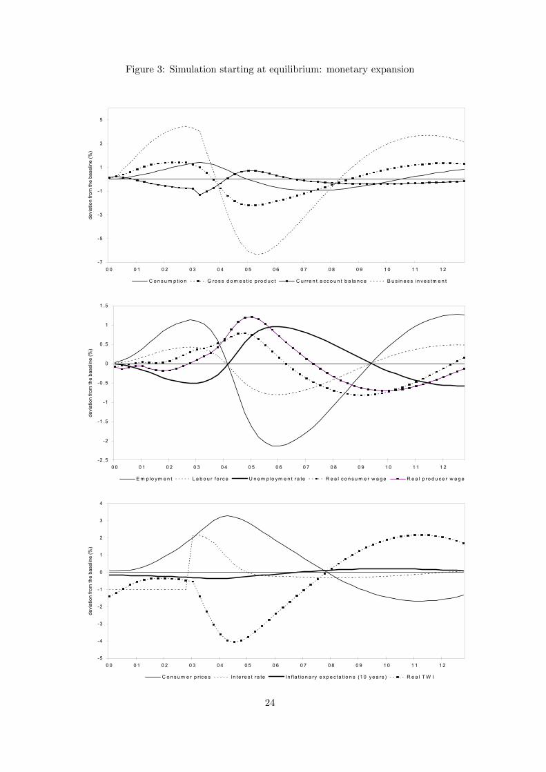
Figure 3: Simulation starting at equilibrium: monetary expansion

-7

-5

-3

-1

1

3

5

0 0 0 1 0 2 0 3 0 4 0 5 0 6 0 7 0 8 0 9 1 0 1 1 1 2

devi

atio

n fro

m th

e ba

selin

e (%

)

C o n s u m p tio n G ro s s d o m e s tic p ro d u c t C u rre n t a c c o u n t b a la n c e B u s in e s s in v e s tm e n t

-2 .5

-2

-1 .5

-1

-0 .5

0

0 .5

1

1 .5

0 0 0 1 0 2 0 3 0 4 0 5 0 6 0 7 0 8 0 9 1 0 1 1 1 2

devi

atio

n fro

m th

e ba

selin

e (%

)

E m p lo y m e n t L a b o u r fo rc e U n e m p lo ym e n t ra te R e a l c o n s u m e r w a g e R e a l p ro d u c e r w a g e

-5

-4

-3

-2

-1

0

1

2

3

4

0 0 0 1 0 2 0 3 0 4 0 5 0 6 0 7 0 8 0 9 1 0 1 1 1 2

devi

atio

n fro

m th

e ba

selin

e (%

)

C o n s u m e r p r ic e s In te re s t ra te In f la t io n a ry e x p e c ta tio n s (1 0 y e a rs ) R e a l T W I

24

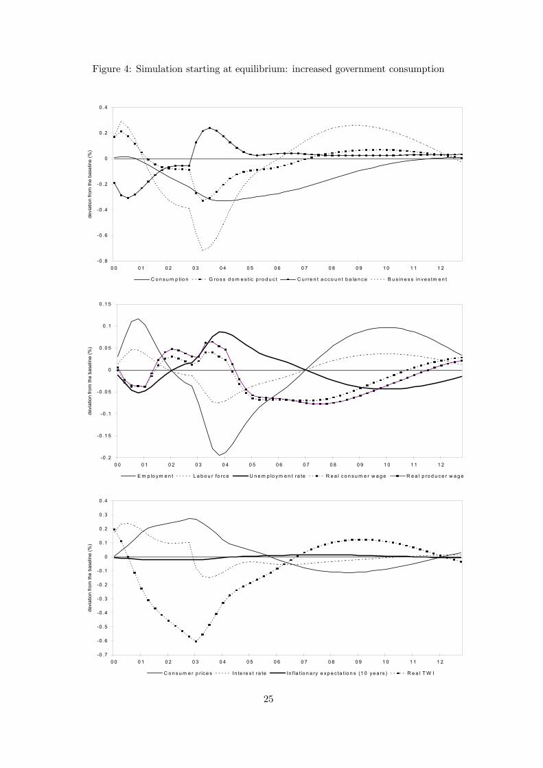
Figure 4: Simulation starting at equilibrium: increased government consumption

-0 .8

-0 .6

-0 .4

-0 .2

0

0 .2

0 .4

0 0 0 1 0 2 0 3 0 4 0 5 0 6 0 7 0 8 0 9 1 0 1 1 1 2

devi

atio

n fro

m th

e ba

selin

e (%

)


-0 .2

-0 .1 5

-0 .1

-0 .0 5

0

0 .0 5

0 .1

0 .1 5

0 0 0 1 0 2 0 3 0 4 0 5 0 6 0 7 0 8 0 9 1 0 1 1 1 2

devi

atio

n fro

m th

e ba

selin

e (%

)

E m p lo ym e n t L a b o u r fo rc e U n e m p lo y m e n t ra te R e a l c o n s u m e r w a g e R e a l p ro d u c e r w a g e

-0 .7

-0 .6

-0 .5

-0 .4

-0 .3

-0 .2

-0 .1

0

0 .1

0 .2

0 .3

0 .4

0 0 0 1 0 2 0 3 0 4 0 5 0 6 0 7 0 8 0 9 1 0 1 1 1 2

devi

atio

n fro

m th

e ba

selin

e (%

)


25

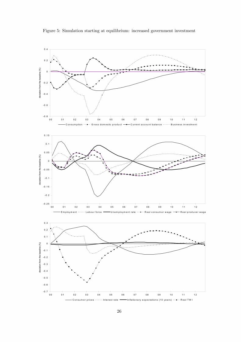
Figure 5: Simulation starting at equilibrium: increased government investment

-0 .8

-0 .6

-0 .4

-0 .2

0

0 .2

0 .4

0 0 0 1 0 2 0 3 0 4 0 5 0 6 0 7 0 8 0 9 1 0 1 1 1 2

devi

atio

n fro

m th

e ba

selin

e (%

)


-0 .2 5

-0 .2

-0 .1 5

-0 .1

-0 .0 5

0

0 .0 5

0 .1

0 .1 5

0 0 0 1 0 2 0 3 0 4 0 5 0 6 0 7 0 8 0 9 1 0 1 1 1 2

devi

atio

n fro

m th

e ba

selin

e (%

)

E m p lo y m e n t L a b o u r fo rc e U n e m p lo y m e n t ra te R e a l c o n s u m e r w a g e R e a l p ro d u c e r w a g e

-0 .7

-0 .6

-0 .5

-0 .4

-0 .3

-0 .2

-0 .1

0

0 .1

0 .2

0 .3

0 0 0 1 0 2 0 3 0 4 0 5 0 6 0 7 0 8 0 9 1 0 1 1 1 2

devi

atio

n fro

m th

e ba

selin

e (%

)


26

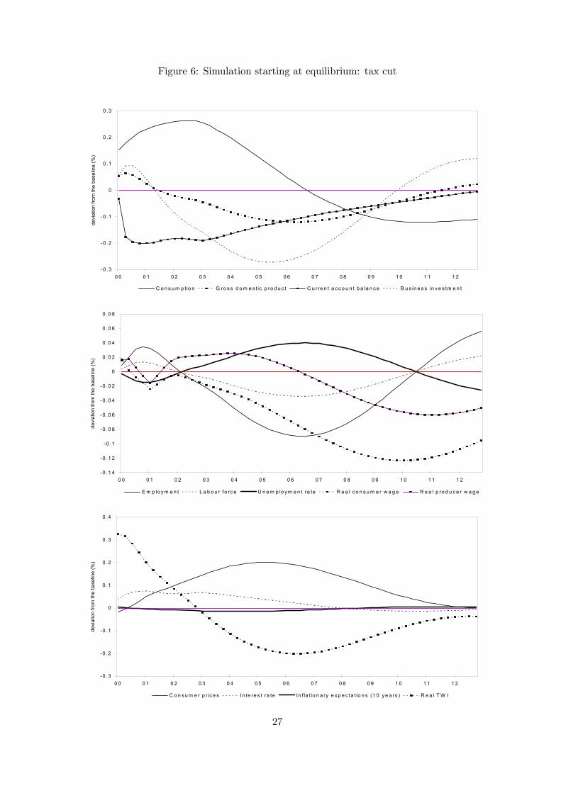
Figure 6: Simulation starting at equilibrium: tax cut

-0 .3

-0 .2

-0 .1

0

0 .1

0 .2

0 .3

0 0 0 1 0 2 0 3 0 4 0 5 0 6 0 7 0 8 0 9 1 0 1 1 1 2

devi

atio

n fro

m th

e ba

selin

e (%

)


-0 .1 4

-0 .1 2

-0 .1

-0 .0 8

-0 .0 6

-0 .0 4

-0 .0 2

0

0 .0 2

0 .0 4

0 .0 6

0 .0 8

0 0 0 1 0 2 0 3 0 4 0 5 0 6 0 7 0 8 0 9 1 0 1 1 1 2

devi

atio

n fro

m th

e ba

selin

e (%

)


-0 .3

-0 .2

-0 .1

0

0 .1

0 .2

0 .3

0 .4

0 0 0 1 0 2 0 3 0 4 0 5 0 6 0 7 0 8 0 9 1 0 1 1 1 2

devi

atio

n fro

m th

e ba

selin

e (%

)


27

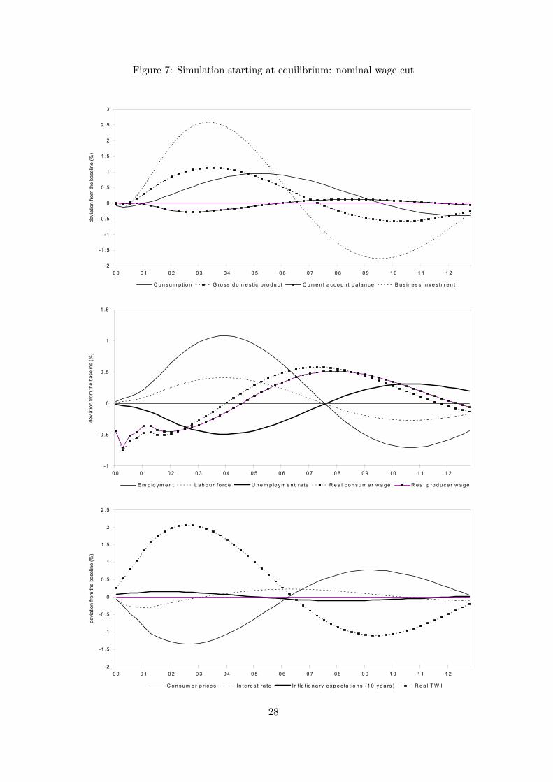
Figure 7: Simulation starting at equilibrium: nominal wage cut

-2

-1 .5

-1

-0 .5

0

0 .5

1

1 .5

2

2 .5

3

0 0 0 1 0 2 0 3 0 4 0 5 0 6 0 7 0 8 0 9 1 0 1 1 1 2

devi

atio

n fro

m th

e ba

selin

e (%

)


-1

-0 .5

0

0 .5

1

1 .5

0 0 0 1 0 2 0 3 0 4 0 5 0 6 0 7 0 8 0 9 1 0 1 1 1 2

devi

atio

n fro

m th

e ba

selin

e (%

)


-2

-1 .5

-1

-0 .5

0

0 .5

1

1 .5

2

2 .5

0 0 0 1 0 2 0 3 0 4 0 5 0 6 0 7 0 8 0 9 1 0 1 1 1 2

devi

atio

n fro

m th

e ba

selin

e (%

)


28

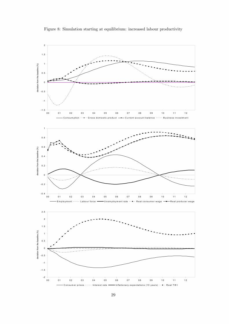
Figure 8: Simulation starting at equilibrium: increased labour productivity

-1 .5

-1

-0 .5

0

0 .5

1

1 .5

2

0 0 0 1 0 2 0 3 0 4 0 5 0 6 0 7 0 8 0 9 1 0 1 1 1 2

devi

atio

n fro

m th

e ba

selin

e (%

)


-0 .4

-0 .2

0

0 .2

0 .4

0 .6

0 .8

1

0 0 0 1 0 2 0 3 0 4 0 5 0 6 0 7 0 8 0 9 1 0 1 1 1 2

devi

atio

n fro

m th

e ba

selin

e (%

)


-2

-1 .5

-1

-0 .5

0

0 .5

1

1 .5

2

2 .5

0 0 0 1 0 2 0 3 0 4 0 5 0 6 0 7 0 8 0 9 1 0 1 1 1 2

devi

atio

n fro

m th

e ba

selin

e (%

)


29

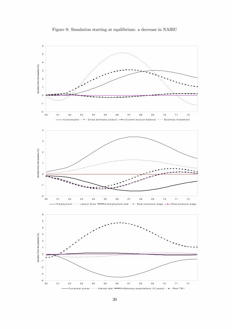
Figure 9: Simulation starting at equilibrium: a decrease in NAIRU

-2

-1

0

1

2

3

4

5

6

0 0 0 1 0 2 0 3 0 4 0 5 0 6 0 7 0 8 0 9 1 0 1 1 1 2

devi

atio

n fro

m th

e ba

selin

e (%

)

C o n s u m p tio n G ro s s d o m e s t ic p ro d u c t C u rre n t a c c o u n t b a la n c e B u s in e s s in v e s tm e n t

-2

-1

0

1

2

3

4

0 0 0 1 0 2 0 3 0 4 0 5 0 6 0 7 0 8 0 9 1 0 1 1 1 2

devi

atio

n fro

m th

e ba

selin

e (%

)


-4

-3

-2

-1

0

1

2

3

4

5

6

0 0 0 1 0 2 0 3 0 4 0 5 0 6 0 7 0 8 0 9 1 0 1 1 1 2

devi

atio

n fro

m th

e ba

selin

e (%

)

C o n s u m e r p r ic e s In te re s t ra te In f la t io n a ry e xp e c ta tio n s (1 0 y e a rs ) R e a l T W I

30

nitude of effect, and the structure of TRYM which lie behind the TRYM simulations

that macroeconomic expansion and wage cuts increase employment in the short run.

Particularly important is the way expectations are modelled. If business, household and

government expectations were fully model consistent rational expectations, the disequi-

librium disturbances caused by the policies would be ignored. In reality forward looking

expectations will vary across decision makers. Sticky wages and prices, and adjustment

costs, extend the disequilibrium period and contribute to cyclical responses driven by

under- and over-shooting the long run equilibrium growth path following policy shocks.

6 Policy simulations starting with high unemployment

This section uses TRYM to simulate the effects of policy options to reduce unemployment

for an economy starting situation with unemployment well above the NAIRU rate. In

particular, it seeks answers to questions of what policy strategies offer a quicker and

more desirable time path of adjustment from a current too high unemployment level to

a longer run equilibrium or NAIRU rate.

In essence, the policy experiments conducted here start with the economy at a dis-

equilibrium point. Since a starting or current unemployment rate above the NAIRU

could be due to many factors, including deficient aggregate demand, too high labour

costs and external and policy shocks, caution will be necessary in drawing general con-

clusions from just one set of simulations. Perhaps more importantly, if the underlying

cause of the starting point disequilibrium is known, one would hypothesise that policy

actions directed at the cause of the disequilibrium would be revealed as better choices.

For example, if the cause of a starting point with too high unemployment was due to a

labour cost increase shock, a priori one would expect simulations to reveal labour cost

restraint to dominate a policy strategy of monetary expansion.

Here we report TRYM policy simulations for the Australian economy from 1992 to

2000. The base or comparison run is the TRYM model estimate of macroeconomic

behaviour over the period with monetary and fiscal policy and international conditions

set at actual values. Simulated GDP, unemployment and consumer and producer prices

closely track actual values. With the base run, unemployment starts at 10.8 per cent

31

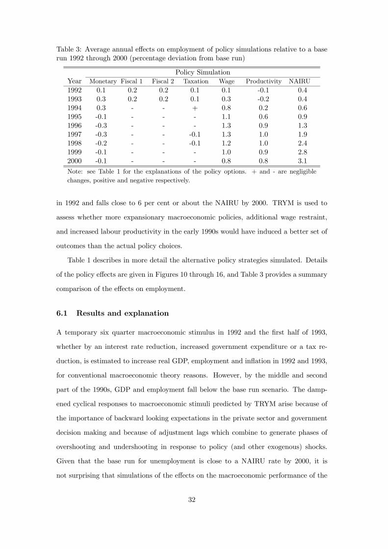
Table 3: Average annual effects on employment of policy simulations relative to a baserun 1992 through 2000 (percentage deviation from base run)

Policy SimulationYear Monetary Fiscal 1 Fiscal 2 Taxation Wage Productivity NAIRU

1992 0.1 0.2 0.2 0.1 0.1 -0.1 0.41993 0.3 0.2 0.2 0.1 0.3 -0.2 0.41994 0.3 - - + 0.8 0.2 0.61995 -0.1 - - - 1.1 0.6 0.91996 -0.3 - - - 1.3 0.9 1.31997 -0.3 - - -0.1 1.3 1.0 1.91998 -0.2 - - -0.1 1.2 1.0 2.41999 -0.1 - - - 1.0 0.9 2.82000 -0.1 - - - 0.8 0.8 3.1

Note: see Table 1 for the explanations of the policy options. + and - are negligible

changes, positive and negative respectively.

in 1992 and falls close to 6 per cent or about the NAIRU by 2000. TRYM is used to

assess whether more expansionary macroeconomic policies, additional wage restraint,

and increased labour productivity in the early 1990s would have induced a better set of

outcomes than the actual policy choices.

Table 1 describes in more detail the alternative policy strategies simulated. Details

of the policy effects are given in Figures 10 through 16, and Table 3 provides a summary

comparison of the effects on employment.

6.1 Results and explanation

A temporary six quarter macroeconomic stimulus in 1992 and the first half of 1993,

whether by an interest rate reduction, increased government expenditure or a tax re-

duction, is estimated to increase real GDP, employment and inflation in 1992 and 1993,

for conventional macroeconomic theory reasons. However, by the middle and second

part of the 1990s, GDP and employment fall below the base run scenario. The damp-

ened cyclical responses to macroeconomic stimuli predicted by TRYM arise because of

the importance of backward looking expectations in the private sector and government

decision making and because of adjustment lags which combine to generate phases of

overshooting and undershooting in response to policy (and other exogenous) shocks.

Given that the base run for unemployment is close to a NAIRU rate by 2000, it is

not surprising that simulations of the effects on the macroeconomic performance of the

32

economy to the different policy packages converge to the base run by 2000.

Lower labour costs are projected to give a large boost to employment for all of the

1990s. Extra employment comes from labour for capital substitution, and also from

greater GDP with increases in investment and net exports which dominate a small

initial fall in private consumption. Adjustment costs and lags mean a slow build-up in

employment through to 1996. By the second part of the 1990s both higher wages and

higher interest rates reduce initial gains in GDP and unemployment and the economy

behaves akin to the base run.

Improved labour productivity initially lowers employment as less employees are re-

quired per unit output, but by 1995 the steady rise in GDP driven by gains in competi-

tiveness lifts employment above the base run. Higher real wages in the late 1990s result

in some fall in the employment gain, but a significant net gain is present in 2000.

The simulation results for the NAIRU shock look strange at the first glance while

all the measures diverge from the base run (see Figure 16). An explanation arises from

the fact that the actual unemployment rate of 10.8 per cent was well above the NAIRU

in 1992. The policy shock is introduced into the wage setting equation (or the Phillips

curve) and the disturbance results in a steady decrease in real wages in the simulation

period. Therefore with a reduction in the NAIRU, employment rises and unemployment

falls constantly. As in the NAIRU simulation starting from the equilibrium path, the

economy should finally settle down at the new NAIRU, but the simulation period is

too short to show cyclical responses converging to the new NAIRU. By the end of the

simulation period (June 2000), the simulated unemployment rate is still 0.4 percentage

points above the new NAIRU, reflecting the very sluggish adjustment properties of the

TRYM model.

A permanent reduction in the NAIRU can be thought of as a permanent wage

cut shock. Since the simulation starts at high unemployment, a wage cut would have

encouraged employers to hire unemployed. As a result, employment and subsequently

economic activity would have risen. The simulation results show the powerfulness of a

NAIRU reduction.

It is difficult to explain the spike in consumer prices in 1992 after several policy

33

shocks. This may be due to residuals or a relative large change in prices.

6.2 Assessment

Policy simulations with TRYM indicate that starting from a high unemployment position

(above its exogenously set NAIRU) active government policy can promote employment

and reduce unemployment. For the particular example of Australia in 1992, our sim-

ulations highlight the virtues of lower labour costs, with production change decisions

dominating a short term loss of household spending power. Expansionary fiscal and

monetary policies help in the short run with the initial expenditure push only partly

crowded out. However, after a few years cyclical responses to macroeconomic policy

stimuli are likely to lead to periods of lower employment and higher unemployment

than otherwise. Small initial falls in employment associated with policies to raise labour

productivity become larger employment gains associated with a larger GDP after three

or so years.

The TRYM simulations point to dampened cyclical responses to the policy changes

rather than a better monotonic adjustment path to the long run equilibrium growth

path. Cyclical responses to policy (and other exogenous) shocks in TRYM simulations

arise because of phases of under- and over-shooting in business and government decisions

associated with imperfect foresight expectations and adjustment costs and lags. While

the precise form and magnitude of cyclical responses will be debatable, nonetheless,

cycles seem more consistent with observed macroeconometric time series than monotonic

responses.

Different responses of the economy to different policy instruments suggest the desir-

ability of a mixture of instruments to assist in reducing unemployment. For example, a

package of programs to raise labour productivity and macroeconomic expansion would

appear to capture important complementarities.

Also important will be choices on the magnitude and timing of the different policy

instruments.

34

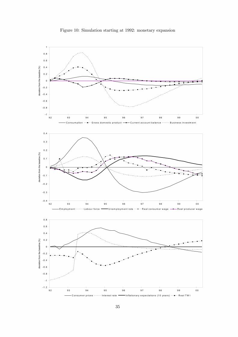
Figure 10: Simulation starting at 1992: monetary expansion

-1

-0 .8

-0 .6

-0 .4

-0 .2

0

0 .2

0 .4

0 .6

0 .8

1

9 2 9 3 9 4 9 5 9 6 9 7 9 8 9 9 0 0

devi

atio

n fro

m th

e ba

selin

e (%

)


-0 .4

-0 .3

-0 .2

-0 .1

0

0 .1

0 .2

0 .3

0 .4

9 2 9 3 9 4 9 5 9 6 9 7 9 8 9 9 0 0

devi

atio

n fro

m th

e ba

selin

e (%

)


-1 .2

-1

-0 .8

-0 .6

-0 .4

-0 .2

0

0 .2

0 .4

0 .6

0 .8

9 2 9 3 9 4 9 5 9 6 9 7 9 8 9 9 0 0

devi

atio

n fro

m th

e ba

selin

e (%

)


35

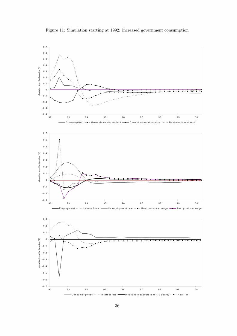
Figure 11: Simulation starting at 1992: increased government consumption

-0 .4

-0 .3

-0 .2

-0 .1

0

0 .1

0 .2

0 .3

0 .4

0 .5

0 .6

0 .7

9 2 9 3 9 4 9 5 9 6 9 7 9 8 9 9 0 0

devi

atio

n fro

m th

e ba

selin

e (%

)


-0 .3

-0 .2

-0 .1

0

0 .1

0 .2

0 .3

0 .4

0 .5

0 .6

0 .7

9 2 9 3 9 4 9 5 9 6 9 7 9 8 9 9 0 0

devi

atio

n fro

m th

e ba

selin

e (%

)


-0 .7

-0 .6

-0 .5

-0 .4

-0 .3

-0 .2

-0 .1

0

0 .1

0 .2

0 .3

9 2 9 3 9 4 9 5 9 6 9 7 9 8 9 9 0 0

devi

atio

n fro

m th

e ba

selin

e (%

)


36

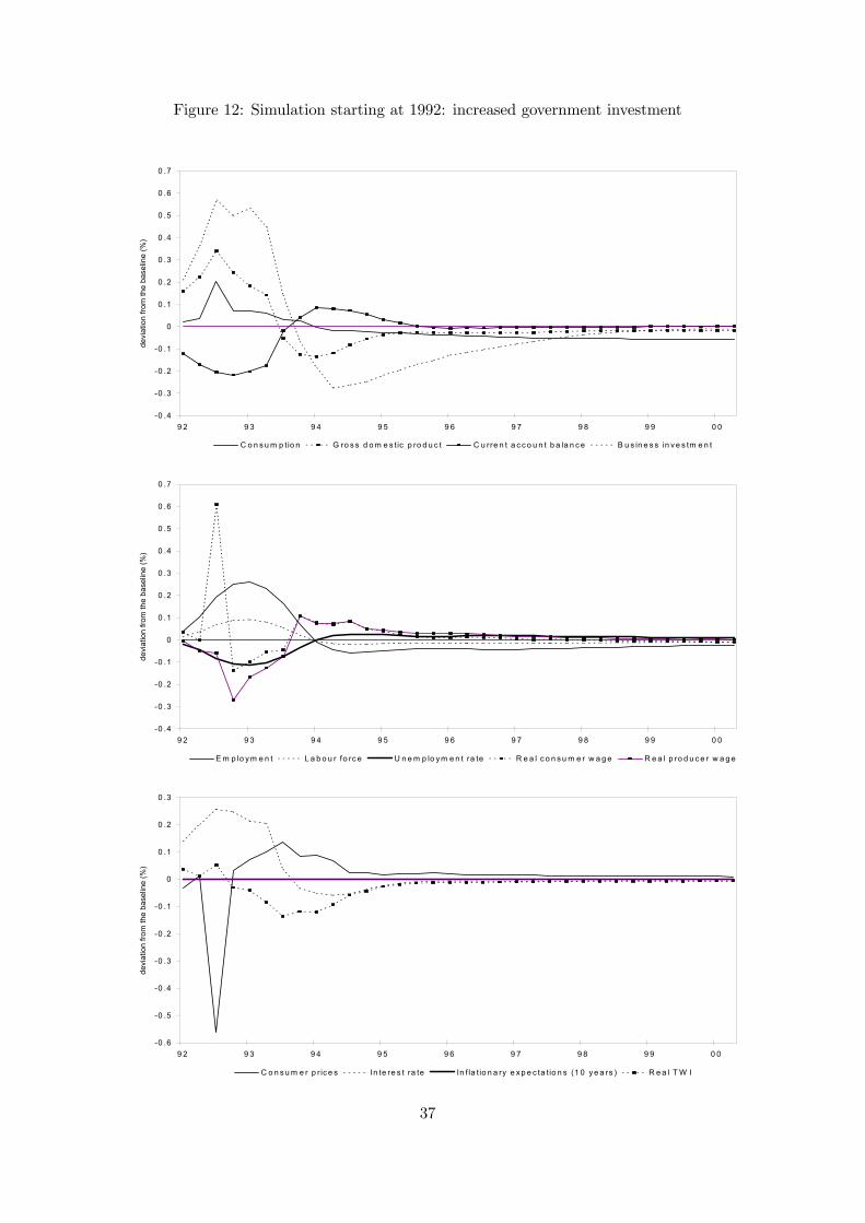
Figure 12: Simulation starting at 1992: increased government investment

-0 .4

-0 .3

-0 .2

-0 .1

0

0 .1

0 .2

0 .3

0 .4

0 .5

0 .6

0 .7

9 2 9 3 9 4 9 5 9 6 9 7 9 8 9 9 0 0

devi

atio

n fro

m th

e ba

selin

e (%

)


-0 .4

-0 .3

-0 .2

-0 .1

0

0 .1

0 .2

0 .3

0 .4

0 .5

0 .6

0 .7

9 2 9 3 9 4 9 5 9 6 9 7 9 8 9 9 0 0

devi

atio

n fro

m th

e ba

selin

e (%

)


-0 .6

-0 .5

-0 .4

-0 .3

-0 .2

-0 .1

0

0 .1

0 .2

0 .3

9 2 9 3 9 4 9 5 9 6 9 7 9 8 9 9 0 0

devi

atio

n fro

m th

e ba

selin

e (%

)


37

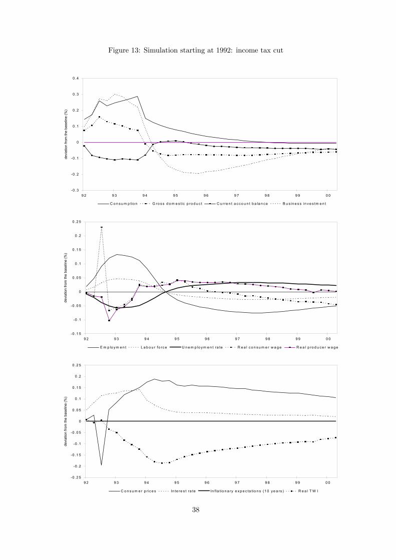
Figure 13: Simulation starting at 1992: income tax cut

-0 .3

-0 .2

-0 .1

0

0 .1

0 .2

0 .3

0 .4

9 2 9 3 9 4 9 5 9 6 9 7 9 8 9 9 0 0

devi

atio

n fro

m th

e ba

selin

e (%

)


-0 .1 5

-0 .1

-0 .0 5

0

0 .0 5

0 .1

0 .1 5

0 .2

0 .2 5

9 2 9 3 9 4 9 5 9 6 9 7 9 8 9 9 0 0

devi

atio

n fro

m th

e ba

selin

e (%

)


-0 .2 5

-0 .2

-0 .1 5

-0 .1

-0 .0 5

0

0 .0 5

0 .1

0 .1 5

0 .2

0 .2 5

9 2 9 3 9 4 9 5 9 6 9 7 9 8 9 9 0 0

devi

atio

n fro

m th

e ba

selin

e (%

)

C o n s u m e r p r ic e s In te re s t ra te In f la t io n a ry e x p e c ta tio n s (1 0 ye a rs ) R e a l T W I

38

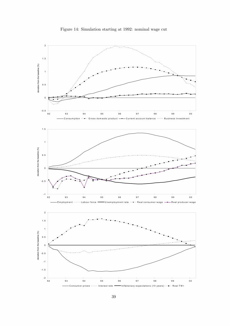
Figure 14: Simulation starting at 1992: nominal wage cut

-0 .5

0

0 .5

1

1 .5

2

9 2 9 3 9 4 9 5 9 6 9 7 9 8 9 9 0 0

devi

atio

n fro

m th

e ba

selin

e (%

)


-1

-0 .5

0

0 .5

1

1 .5

9 2 9 3 9 4 9 5 9 6 9 7 9 8 9 9 0 0

devi

atio

n fro

m th

e ba

selin

e (%

)


-2

-1 .5

-1

-0 .5

0

0 .5

1

1 .5

2

9 2 9 3 9 4 9 5 9 6 9 7 9 8 9 9 0 0

devi

atio

n fro

m th

e ba

selin

e (%

)


39

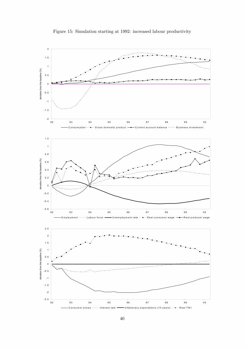
Figure 15: Simulation starting at 1992: increased labour productivity

-2

-1 .5

-1

-0 .5

0

0 .5

1

1 .5

2

9 2 9 3 9 4 9 5 9 6 9 7 9 8 9 9 0 0

devi

atio

n fro

m th

e ba

selin

e (%

)


-0 .6

-0 .4

-0 .2

0

0 .2

0 .4

0 .6

0 .8

1

1 .2

9 2 9 3 9 4 9 5 9 6 9 7 9 8 9 9 0 0

devi

atio

n fro

m th

e ba

selin

e (%

)


-2 .5

-2

-1 .5

-1

-0 .5

0

0 .5

1

1 .5

2

2 .5

9 2 9 3 9 4 9 5 9 6 9 7 9 8 9 9 0 0

devi

atio

n fro

m th

e ba

selin

e (%

)


40

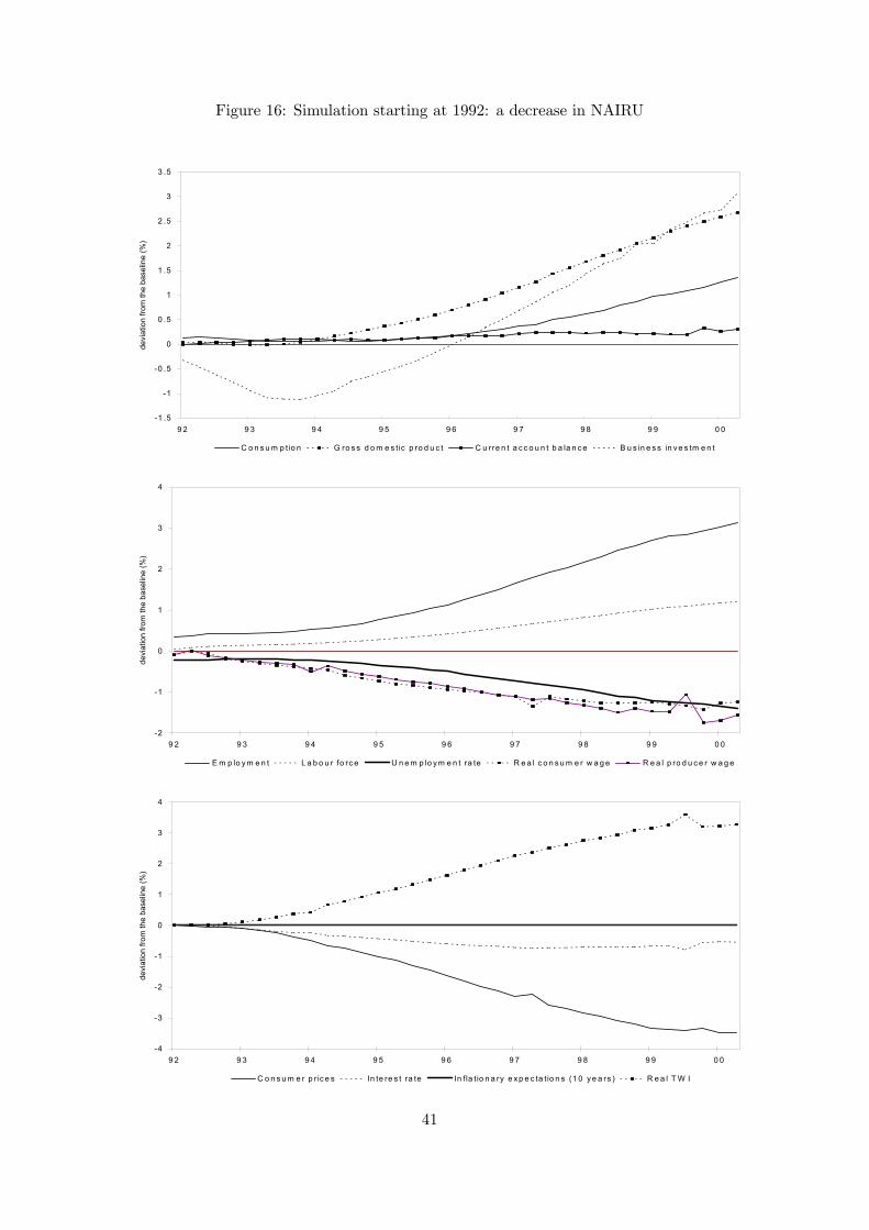
Figure 16: Simulation starting at 1992: a decrease in NAIRU

-1 .5

-1

-0 .5

0

0 .5

1

1 .5

2

2 .5

3

3 .5

9 2 9 3 9 4 9 5 9 6 9 7 9 8 9 9 0 0

devi

atio

n fro

m th

e ba

selin

e (%

)


-2

-1

0

1

2

3

4

9 2 9 3 9 4 9 5 9 6 9 7 9 8 9 9 0 0

devi

atio

n fro

m th

e ba

selin

e (%

)


-4

-3

-2

-1

0

1

2

3

4

9 2 9 3 9 4 9 5 9 6 9 7 9 8 9 9 0 0

devi

atio

n fro

m th

e ba

selin

e (%

)

C o n s u m e r p r ic e s In te re s t ra te In f la t io n a ry e xp e c ta tio n s (1 0 y e a rs ) R e a l T W I

41

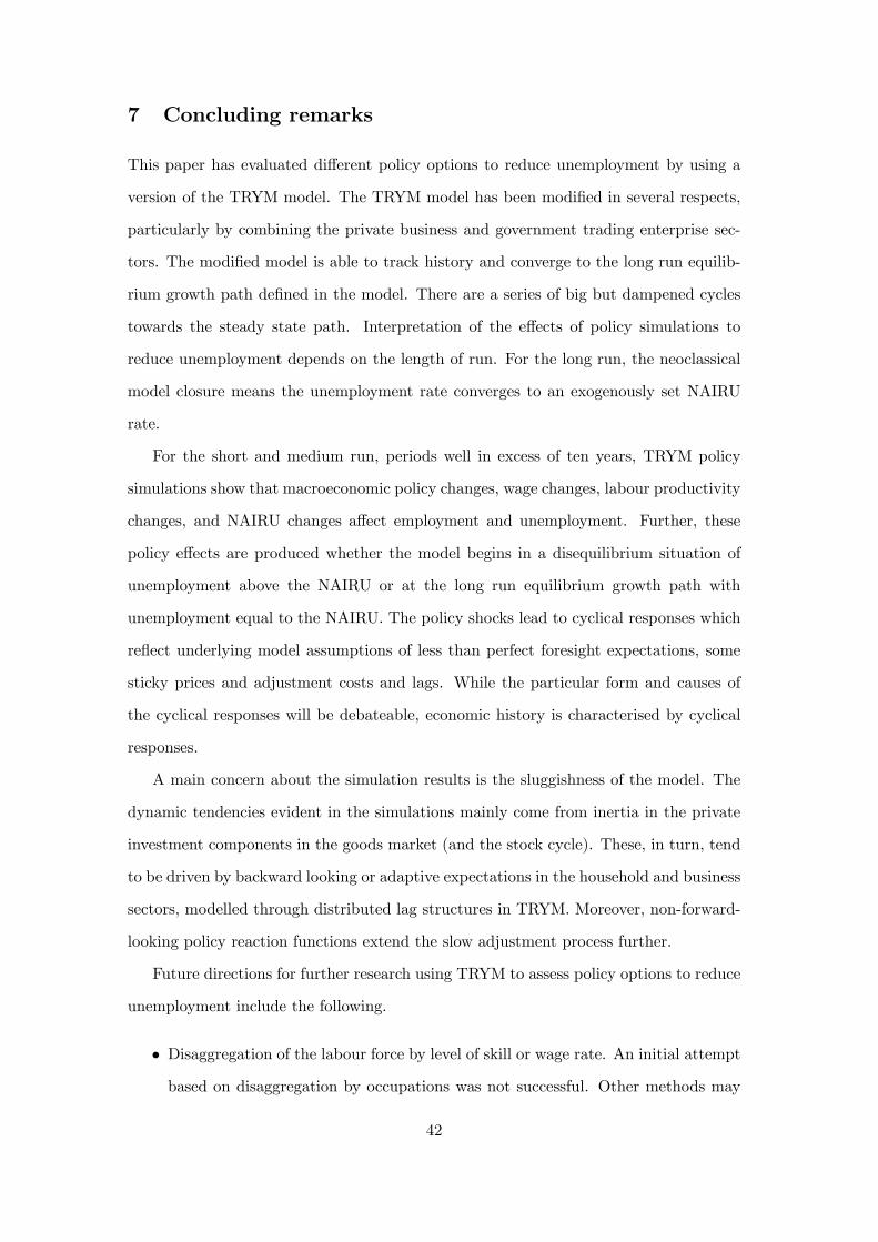
7 Concluding remarks

This paper has evaluated different policy options to reduce unemployment by using a

version of the TRYM model. The TRYM model has been modified in several respects,

particularly by combining the private business and government trading enterprise sec-

tors. The modified model is able to track history and converge to the long run equilib-

rium growth path defined in the model. There are a series of big but dampened cycles

towards the steady state path. Interpretation of the effects of policy simulations to

reduce unemployment depends on the length of run. For the long run, the neoclassical

model closure means the unemployment rate converges to an exogenously set NAIRU

rate.

For the short and medium run, periods well in excess of ten years, TRYM policy

simulations show that macroeconomic policy changes, wage changes, labour productivity

changes, and NAIRU changes affect employment and unemployment. Further, these

policy effects are produced whether the model begins in a disequilibrium situation of

unemployment above the NAIRU or at the long run equilibrium growth path with

unemployment equal to the NAIRU. The policy shocks lead to cyclical responses which

reflect underlying model assumptions of less than perfect foresight expectations, some

sticky prices and adjustment costs and lags. While the particular form and causes of

the cyclical responses will be debateable, economic history is characterised by cyclical

responses.

A main concern about the simulation results is the sluggishness of the model. The

dynamic tendencies evident in the simulations mainly come from inertia in the private

investment components in the goods market (and the stock cycle). These, in turn, tend

to be driven by backward looking or adaptive expectations in the household and business

sectors, modelled through distributed lag structures in TRYM. Moreover, non-forward-

looking policy reaction functions extend the slow adjustment process further.

Future directions for further research using TRYM to assess policy options to reduce

unemployment include the following.

• Disaggregation of the labour force by level of skill or wage rate. An initial attemptbased on disaggregation by occupations was not successful. Other methods may

42

be worthwhile to pursue in the future. One option is to obtain sensible estimates

of the elasticities of substitution among different factors (i.e., capital, skilled and

unskilled labour) from the existing literature, and then to calibrate the labour

market equations in TRYM. The calibrated model can be used to evaluate policy

options.

• Production functions. As identified in Harding and Song (2001), the spill-overeffects of government capital stock in private production needs to be addressed.

• Others. The TRYM model may be improved in other areas. These include the

policy reaction mechanisms, the labour market block and the money demand equa-

tion.

References

Australian Bureau of Statistics (1997): ASCO : Australian Standard Classifica-

tion of Occupations. Australian Bureau of Statistics, Canberra, second edn., Catalogue

no. 1220.0.

Commonwealth Treasury (1996a): “Documentation of the Treasury Macroeconomic

(TRYM) Model of the Australian Economy,” Discussion paper, Macroeconomic Anal-

ysis Branch, Commonwealth Treasury.

(1996b): “The Macroeconomics of the TRYM Model,” Discussion paper,

Macroeconomic Analysis Branch, Commonwealth Treasury.

Downes, P., and K. Bernie (1999): “The Macroeconomics of Unemployment in the

Treasury Macroeconomic (TRYM) Model,” TRYM Related Paper 20, Commonwealth

Treasury.

Dungey, M., and A. Pagan (2000): “A Structural VAR Model of the Australian

Economy,” Economic Record, 76, 321—42.

43




https://www.researchgate.net/publication/5058678_Towards_a_Strucrural_VAR_Model_of_the_Australian_Economy?el=1_x_8&enrichId=rgreq-8289fdf7b0db0a28624960f29daea21a-XXX&enrichSource=Y292ZXJQYWdlOzUxMDMzNjU7QVM6OTg3NjE2OTUwMzk0OThAMTQwMDU1ODAzMTc5OA==

https://www.researchgate.net/publication/5058678_Towards_a_Strucrural_VAR_Model_of_the_Australian_Economy?el=1_x_8&enrichId=rgreq-8289fdf7b0db0a28624960f29daea21a-XXX&enrichSource=Y292ZXJQYWdlOzUxMDMzNjU7QVM6OTg3NjE2OTUwMzk0OThAMTQwMDU1ODAzMTc5OA==

Fair, R. C., and J. Taylor (1983): “Solution and Maximum Likelihood Estimation of

Dynamic Non-Linear Rational Expectations Models,” Econometrica, 51, pp. 139—78.

Harding, D., and L. L. Song (2001): “Simulation Properties of TRYM: Evaluation

and Modification,” unpublished manuscript.

Layard, R., S. Nickell, and R. Jackman (1991): Unemployment: Macroeconomic

Performance and the Labour Market. Oxford University Press, Oxford.

Song, L. L., and E. Webster (2001): “How Segmented Are Skilled and Unskilled

Labour Markets: The Case of Beveridge Curves,” Working paper 14/01, Melbourne

Institute of Applied Economic and Social Research, The University of Melbourne

(http://www.melbourneinstitute.com).

Summers, P. (2001): “Forecasting Australia’s Economic Performance During the Asian

Crisis,” International Journal of Forecasting, 17, 499—515.

Thomson, J. (2000): “The Labour Market in Macroeconomic Models of the Australian

Economy,” Working Paper 18/00, Melbourne Institute of Applied Economic and So-

cial Research, The University of Melbourne (http://www.melbourneinstitute.com).

44

https://www.researchgate.net/publication/222190937_Forecasting_Australia's_economic_performance_during_the_Asian_crisis?el=1_x_8&enrichId=rgreq-8289fdf7b0db0a28624960f29daea21a-XXX&enrichSource=Y292ZXJQYWdlOzUxMDMzNjU7QVM6OTg3NjE2OTUwMzk0OThAMTQwMDU1ODAzMTc5OA==

https://www.researchgate.net/publication/222190937_Forecasting_Australia's_economic_performance_during_the_Asian_crisis?el=1_x_8&enrichId=rgreq-8289fdf7b0db0a28624960f29daea21a-XXX&enrichSource=Y292ZXJQYWdlOzUxMDMzNjU7QVM6OTg3NjE2OTUwMzk0OThAMTQwMDU1ODAzMTc5OA==

https://www.researchgate.net/publication/4895282_Solution_and_Maximum_Likelihood_Estimation_of_Dynamic_Non-Linear_Rational_Expectations_Models?el=1_x_8&enrichId=rgreq-8289fdf7b0db0a28624960f29daea21a-XXX&enrichSource=Y292ZXJQYWdlOzUxMDMzNjU7QVM6OTg3NjE2OTUwMzk0OThAMTQwMDU1ODAzMTc5OA==

https://www.researchgate.net/publication/4895282_Solution_and_Maximum_Likelihood_Estimation_of_Dynamic_Non-Linear_Rational_Expectations_Models?el=1_x_8&enrichId=rgreq-8289fdf7b0db0a28624960f29daea21a-XXX&enrichSource=Y292ZXJQYWdlOzUxMDMzNjU7QVM6OTg3NjE2OTUwMzk0OThAMTQwMDU1ODAzMTc5OA==





https://www.researchgate.net/publication/5103341_The_Labour_Market_in_Macroeconomic_Models_of_the_Australian_Economy?el=1_x_8&enrichId=rgreq-8289fdf7b0db0a28624960f29daea21a-XXX&enrichSource=Y292ZXJQYWdlOzUxMDMzNjU7QVM6OTg3NjE2OTUwMzk0OThAMTQwMDU1ODAzMTc5OA==



https://www.researchgate.net/publication/227467347_Unemployment_Macroeconomic_Performance_and_the_Labour_Market?el=1_x_8&enrichId=rgreq-8289fdf7b0db0a28624960f29daea21a-XXX&enrichSource=Y292ZXJQYWdlOzUxMDMzNjU7QVM6OTg3NjE2OTUwMzk0OThAMTQwMDU1ODAzMTc5OA==

https://www.researchgate.net/publication/227467347_Unemployment_Macroeconomic_Performance_and_the_Labour_Market?el=1_x_8&enrichId=rgreq-8289fdf7b0db0a28624960f29daea21a-XXX&enrichSource=Y292ZXJQYWdlOzUxMDMzNjU7QVM6OTg3NjE2OTUwMzk0OThAMTQwMDU1ODAzMTc5OA==

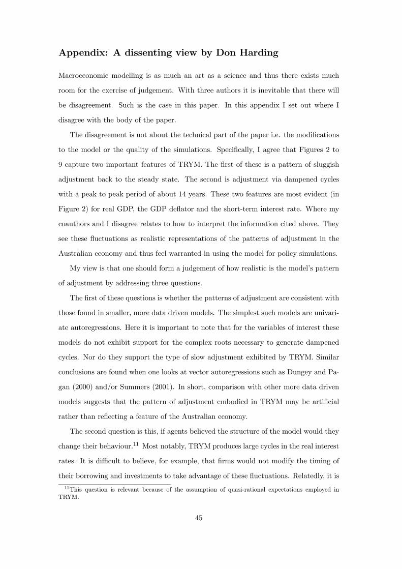
Appendix: A dissenting view by Don Harding

Macroeconomic modelling is as much an art as a science and thus there exists much

room for the exercise of judgement. With three authors it is inevitable that there will

be disagreement. Such is the case in this paper. In this appendix I set out where I

disagree with the body of the paper.

The disagreement is not about the technical part of the paper i.e. the modifications

to the model or the quality of the simulations. Specifically, I agree that Figures 2 to

9 capture two important features of TRYM. The first of these is a pattern of sluggish

adjustment back to the steady state. The second is adjustment via dampened cycles

with a peak to peak period of about 14 years. These two features are most evident (in

Figure 2) for real GDP, the GDP deflator and the short-term interest rate. Where my

coauthors and I disagree relates to how to interpret the information cited above. They

see these fluctuations as realistic representations of the patterns of adjustment in the

Australian economy and thus feel warranted in using the model for policy simulations.

My view is that one should form a judgement of how realistic is the model’s pattern

of adjustment by addressing three questions.

The first of these questions is whether the patterns of adjustment are consistent with

those found in smaller, more data driven models. The simplest such models are univari-

ate autoregressions. Here it is important to note that for the variables of interest these

models do not exhibit support for the complex roots necessary to generate dampened

cycles. Nor do they support the type of slow adjustment exhibited by TRYM. Similar

conclusions are found when one looks at vector autoregressions such as Dungey and Pa-

gan (2000) and/or Summers (2001). In short, comparison with other more data driven

models suggests that the pattern of adjustment embodied in TRYM may be artificial

rather than reflecting a feature of the Australian economy.

The second question is this, if agents believed the structure of the model would they

change their behaviour.11 Most notably, TRYM produces large cycles in the real interest

rates. It is difficult to believe, for example, that firms would not modify the timing of

their borrowing and investments to take advantage of these fluctuations. Relatedly, it is

11This question is relevant because of the assumption of quasi-rational expectations employed inTRYM.

45

difficult to believe that the RBA would be content with the pattern of price movements

shown in Figure 2 and this suggests that the assumed monetary policy reaction function

does not adequately describe that used by the RBA.

The third question to ask is whether the pattern of adjustments is consistent with

broad facts about the economy. One of these is that recessions are difficult to forecast

(see Economics Focus, Say “R”, The Economist, 1-7 Dec 2001 for recent evidence on

this). But inspection of Figure 7 shows that TRYM suggests a sufficiently large deviation

of GDP below trend in about 2007 to be consistent with a recession in 2007. Is it likely

that we can see use models to this far into the future? I think not. And this also leads

me to question whether TRYM adequately represents the dynamics of the Australian

macroeconomy.

46

Policy Options to Reduce Unemployment: TRYM Simulations

Documents