Policy interactions, risk and price formation in carbon markets

1

Policy interactions, risk and price

formation in carbon markets

William Blyth1, Derek Bunn2 , Janne Kettunen2, Tom Wilson3

1. Oxford Energy Associates, Wheatley Road, Forest Hill, Oxford OX33 1EH, UK

2. London Business School, Regent's Park, London NW1 4SA, UK

3. Electric Power Research Institute, 3420 Hillview Avenue, Palo Alto, CA 94304-1395 USA

Abstract Carbon pricing is an important mechanism for signalling to individuals and companies societal

concerns about climate change, and for providing an incentive to invest in carbon abatement. Price

formation in carbon markets involves a complex interplay between policy targets, dynamic

technology costs, and market rules. Carbon pricing may under-deliver investment due to R&D

externalities and so additional policies may be needed which themselves affect carbon price

formation. Also, future abatement costs depend on the extent of technology deployment due to

learning-by-doing, leading to some circularity in the analysis of investment, learning, costs and

prices. This paper introduces an analytical framework based on marginal abatement cost (MAC)

curves with the aim of providing an intuitive (rather than complete) understanding of the key

dynamics and risk factors in carbon markets. The framework extends the usual static MAC

representation of the market to incorporate policy interactions and some technology cost dynamics.

The analysis indicates that supporting large-scale deployment of mature abatement technologies

suppresses the marginal cost of abatement, sometimes to zero, whilst increasing total abatement

costs. However, support for early stage R&D may reduce both total abatement cost and carbon

price risk. It is anticipated that the intuitive framework introduced here may help in policy design

issues around cost containment measures and other market design options such as banking and

borrowing (factors that are not currently incorporated into the model).

Introduction Addressing the twin challenges of energy security and climate change will require a major shift in

investment behaviour in the energy sector over the coming decades (IEA 2003, 2008a). This

represents a significant challenge not only because of the scale of the transformation required away

from the existing energy infrastructure, but also because this has to be undertaken in the context of

substantial additional risks due to policy as well as the enhanced concerns about credit and business

performance. The policy-formation risks relate, inter alia, to the rate at which international collective

actions can be agreed, as well as uncertainties on a range of related factors such as the baseline rate

of growth of unmitigated emissions and the cost and availability of abatement options. Policy-

makers therefore need to be adaptive to changing circumstances, whilst at the same time trying to

2

create conditions in their own jurisdictions for motivating private capital towards low-carbon

investment in a period of enhanced concerns about investment risks in general.

Carbon pricing (either through taxes or tradable permits) is seen as a necessary though not sufficient

element of the policy package to create suitable investment incentives (Stern 2006), since market

externalities mean that carbon pricing on its own may tend to under-deliver investment in research

and development of new technologies (Rosendahl 2004). This means that other policy mechanisms

are required in addition to pricing mechanisms. However, interactions between these multiple

policies can undermine the overall efficiency of climate policy (Sorrell 2003), leading to a number of

open questions as to how to design and coordinate multiple climate policies.

Another important factor to address is price risk. Risk is an inevitable consequence of the underlying

uncertainties in the economics and science of climate change, and the presence of risk in carbon

markets does not equate to a market failure. Nevertheless, risk does affect investment behaviour,

and is affected by market design. Policy-makers therefore need to take risk into account when

designing carbon markets, and when forming expectations about the extent to which investment

decision-makers will respond to carbon market price signals. Likewise, companies will need to

understand the key drivers and risk factors when formulating their investment and trading

strategies.

Two questions this paper aims to address in particular are:

• What is the impact of policy uncertainty and technology cost uncertainty on price risk in a

carbon market?

• How do technology-specific policies interact with carbon price signals?

The first question arises because carbon price risk is an important factor in investment decision-

making by energy companies. Kiriyama 2004 looks at the effects of carbon price and other

uncertainties on the value of nuclear power assets and impacts, and shows that risk raises the

financial threshold for investment decisions. Reedman 2006 looks at the effect of uncertainty on the

timing of various electricity generation technologies, and found that uptake varied significantly

depending on investor’s view of the risks. Roques 2006 identifies that the hedging role of nuclear

power may affect technology choice under conditions of uncertain gas and carbon prices, whilst

Rothwell 2006 identifies a significant risk premium for new investment associated with various

uncertainties in the financial case for nuclear power. Blyth 2007 and Yang 2008 identify the effects

of carbon price risk on investment decisions, showing that, whilst for baseload plant, fuel price risks

are often more significant, that carbon price risks are still significant for the low-carbon technology

options. There is also a significant body of more generalised research on how to manage risks in

market-based mechanisms for pollution control (for a review see Cropper 1992, also Kling 1997).

Some of this research focuses on the choice under uncertainty between price-based instruments

(taxes) vs. quantity-based instruments (emissions trading), for example Weitzman 1974, Newell

2003, Krysiak 2008, Mandell 2008. Another focus is on design options for constraining price risk in

emissions trading schemes, for example price caps and/or price floors (see for example Pizer 2002,

Hepburn 2006).

3

Despite a few studies that look empirically at carbon price risks and the efficacy of the price signal

based on the operation of the EU-ETS since 2005 (e.g. Ellerman 2007), most research on this theme

uses quite a stylised representation of carbon price uncertainty, which limits the practical

application of the policy recommendations. In general, models of price risk in the EU carbon market

have been developed that focus on the abatement options which are expected to be key drivers of

the carbon price. For example Seifert 2008 and Chesney 2008 consider carbon prices to be

determined by the marginal cost of switching fuel, and so model variability as a function of gas and

coal price variability. In contrast, because current carbon allowances are bankable in the EU-ETS,

Lewis 2008 assumes future prices will ultimately be determined by the cost of clean coal technology,

and uses discounting to arrive at an estimate of the current value of allowances.

This paper builds on these approaches by including a more complete description of the different

abatement technologies within the EU-ETS, and including the impact of technology cost dynamics

and policy uncertainty. By taking a more holistic and long-term view of carbon market drivers than

previous studies, this paper shows how the structure of the carbon market will change as the energy

sector evolves, and suggests that the risk characteristics of the carbon market are dependent on

climate policy scenarios. In order to characterise risk it is necessary to account for the range of

values for the various drivers in the market, and the influence of each of these drivers on the range

carbon prices. The problem therefore lends itself to a dynamic stochastic modelling approach,

which we develop below. The model results indicate that a shift from a 20% EU-wide abatement

scenario to a 30% EU-wide abatement scenario (with a corresponding tightening of the level of the

EU-ETS cap) would have a significant effect not only on the expected level of the carbon price, but

would also alter the fundamental drivers of the carbon price, since switching from coal to gas would

no longer be the dominant marginal abatement technology, breaking the link between gas price and

carbon price.

The second question (How do technology-specific policies interact with carbon price signals?) is

crucial because of the need to manage interactions between technology-specific policies such as

standards and subsidies, with nondiscriminatory market mechanisms, such as cap-and trade. Both

types of policy are needed. Clarke 2006 identifies the key mechanisms that drive technological

change, notably learning-by-doing, R&D and spillover effects, and these can have an important

effect in reducing the cost of abatement (Baker 2008, Gillingham 2008). It is difficult, however, for

carbon prices, which are volatile, to credibly guarantee the high future prices that justify current

expenditure on R&D into new technologies (Helm 2003). In consequence, there is evidence that in

the presence of multiple market externalities, multiple policy measures may perform better than

single policy measures. Goulder 2000 shows that the presence of induced technological change will

reduce the cost of achieving a given environmental outcome. This reduction in costs can be used to

justify additional policies to promote knowledge accumulation through R&D and learning-by-doing.

Rosendahl 2004 shows that optimal tax rates should be differentiated to reflect the capacity for

learning, and will therefore not necessarily be the same across all sources, contrary to the standard

assumption of environmental economics; a result also found in Richels 2008 and Otto 2008. Fischer

2008a finds that technology policy is only effective if there is a significant carbon price signal in

place, and shows how different policy instruments perform in terms of the cost of emissions

reductions in the presence of R&D externalities (in particular spillover effects which prevent private

companies appropriating all the benefits of R&D expenditure). They show that an optimal portfolio

4

of policies achieves emission reductions at a significantly lower cost than any single policy, although

the bulk of the emission reductions occur due to the emissions pricing element of the policy

package.

Managing such an optimal portfolio in practice is complicated by interactions between these

policies. Introducing financial support in addition to the carbon price signal in order to stimulate

uptake of new technologies will tend to suppress the carbon price because it reduces the level of

abatement required from emissions sources within the trading scheme. It is therefore possible that

policy-making succumbs to a self-fulfilling prophesy whereby carbon markets are deemed to be

insufficient on their own, justifying more and more additional policy measures which further

undermine the efficacy of the carbon market instrument. A prominent illustration of some of the

problems of policy interactions and risk is provided by the EU (European Commission 2008) which

includes provisions for strengthening the EU emissions trading scheme (EU-ETS), an ambitious target

of 20% of final energy consumption to come from renewable sources by 2020, targets for improved

energy efficiency, as well as a support package for carbon capture and storage. Because they all

tackle emissions from the same key sources, there is significant scope for these wide-ranging and

potentially transformative policies to interact in a way which reduces their individual efficacy

(Stankeviciute 2008). The direction and magnitude of these interactions is taken into account for

example in the EU’s energy modelling exercises (EU Commission 2008a), which shows a relatively

modest depression in the carbon price resulting from the introduction of the 20% renewable energy

target. However, all these scenario analyses are static, and do not take account of the wide range of

uncertainties and path-dependent consequences that drive the carbon price. The results in this

paper show that if there is expected to be significant scope for technological learning, supporting

early stage technology development can reduce the range of uncertainty in future carbon prices as

well as overall abatement costs. On the other hand, supporting large-scale deployment through

separate technology policies will tend not only to suppress the mean expected carbon price, but can

lead to a significant probability of reducing the carbon price to a very low value. Such an occurrence

would tend to widen the price differential between the carbon market and the supplementary

support mechanisms. This would lead investors to become more reliant on the continuation of those

support mechanisms, with consequently greater market fragmentation and reduced scope for policy

integration. .

The authors are aware of a certain circularity in the arguments around price formation, risk,

marginal cost, investment levels and learning. For example, all else equal, an increase in the carbon

price leads to greater levels of investment, increased technological learning, reduced marginal cost

and a reduction in carbon price! Such circularity could formally be resolved in an equilibrium model

that fully endogenised these feedback mechanisms. The approach taken in this paper on the other

hand takes a partial equilibrium approach which does not endogenise technology costs or

abatement quanties, but takes these as exogenous inputs to the model. These limitations mean that

the current model output may best be viewed as ‘raw’ data for input into subsequent analysis,

rather than an end in itself.

For example, the current model is designed to look at underlying price drivers and risk factors, not

actual carbon price risks per se. Carbon prices in real markets will depend on a number of important

additional features of the market such as banking and borrowing of allowances between years, and

5

the inclusion of cost containment measures such as price ceilings and floors which are not included

in the model. By omitting these policy design features, the model output presented here provides

‘raw’ data on underlying marginal cost drivers which can inform subsequent analysis on potential

price behaviour in markets where these policy design features are included.

It should also be noted that the price risks implied by the current model would need to be fed into a

separate investment model to look at the implications for investment risk and technology choice.

These risks are not taken into account inside the current model when calculating the marginal cost

of abatement of a particular technology, but such feedbacks could in principle be incorporated

through iterative model running.

Despite the limitations of partial equilibrium analyses, they do have some advantages in providing

transparency and intuition, and the relatively simple structure of this model facilitates a stochastic

analysis suitable for investigating risk and uncertainty. Providing this intuition, together with ‘raw’

data on the potential dispersion of marginal costs of abatement for subsequent risk analysis is

considered to be the main contribution of this paper.

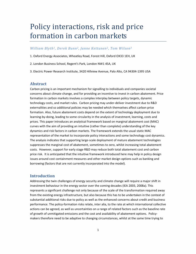
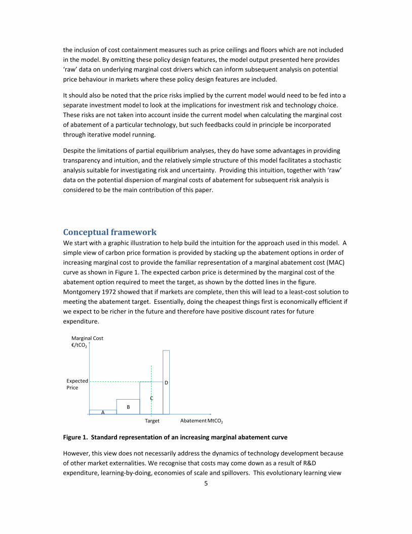
Conceptual framework We start with a graphic illustration to help build the intuition for the approach used in this model. A

simple view of carbon price formation is provided by stacking up the abatement options in order of

increasing marginal cost to provide the familiar representation of a marginal abatement cost (MAC)

curve as shown in Figure 1. The expected carbon price is determined by the marginal cost of the

abatement option required to meet the target, as shown by the dotted lines in the figure.

Montgomery 1972 showed that if markets are complete, then this will lead to a least-cost solution to

meeting the abatement target. Essentially, doing the cheapest things first is economically efficient if

we expect to be richer in the future and therefore have positive discount rates for future

expenditure.

AB

C

D

Abatement MtCO2Target

Marginal Cost

€/tCO2

Expected

Price

Figure 1. Standard representation of an increasing marginal abatement curve

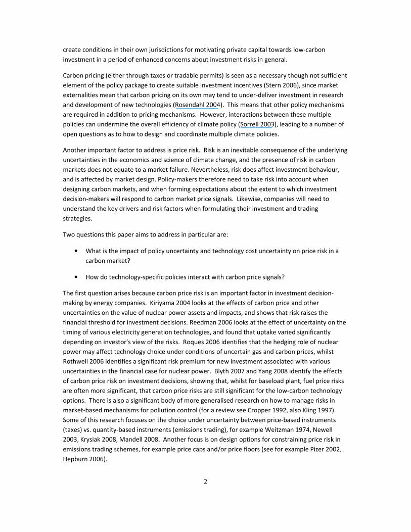
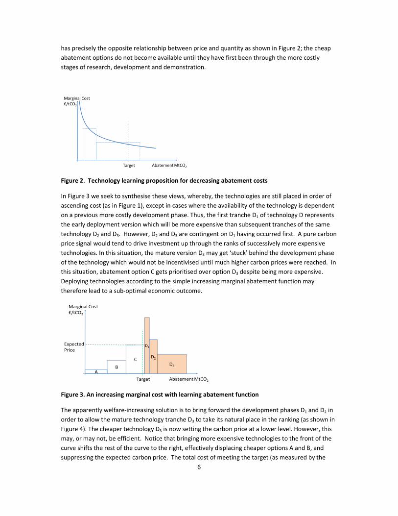
However, this view does not necessarily address the dynamics of technology development because

of other market externalities. We recognise that costs may come down as a result of R&D

expenditure, learning-by-doing, economies of scale and spillovers. This evolutionary learning view

6

has precisely the opposite relationship between price and quantity as shown in Figure 2; the cheap

abatement options do not become available until they have first been through the more costly

stages of research, development and demonstration.

Abatement MtCO2Target

Marginal Cost

€/tCO2

Figure 2. Technology learning proposition for decreasing abatement costs

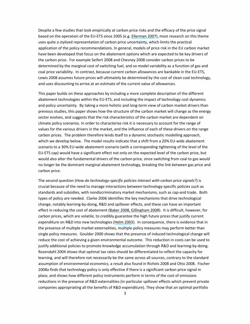
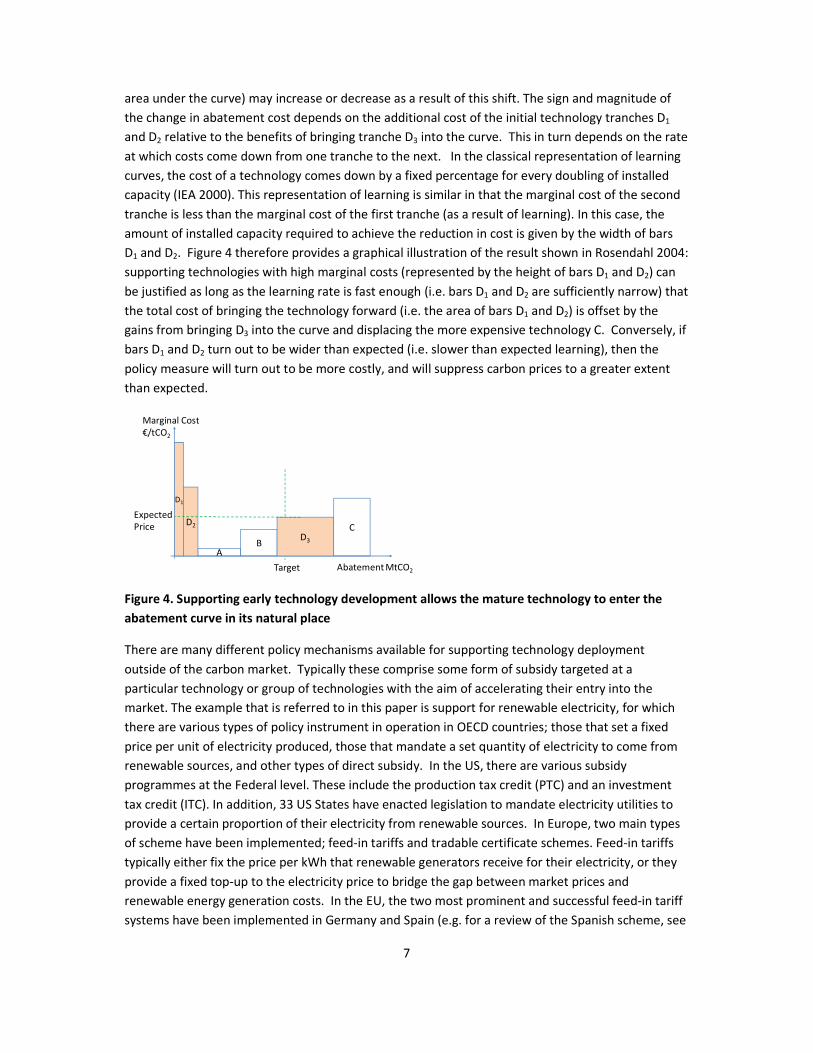
In Figure 3 we seek to synthesise these views, whereby, the technologies are still placed in order of

ascending cost (as in Figure 1), except in cases where the availability of the technology is dependent

on a previous more costly development phase. Thus, the first tranche D1 of technology D represents

the early deployment version which will be more expensive than subsequent tranches of the same

technology D2 and D3. However, D2 and D3 are contingent on D1 having occurred first. A pure carbon

price signal would tend to drive investment up through the ranks of successively more expensive

technologies. In this situation, the mature version D3 may get ‘stuck’ behind the development phase

of the technology which would not be incentivised until much higher carbon prices were reached. In

this situation, abatement option C gets prioritised over option D3 despite being more expensive.

Deploying technologies according to the simple increasing marginal abatement function may

therefore lead to a sub-optimal economic outcome.

AB

C

D1

Abatement MtCO2Target

Marginal Cost

€/tCO2

Expected

Price

D3

D2

Figure 3. An increasing marginal cost with learning abatement function

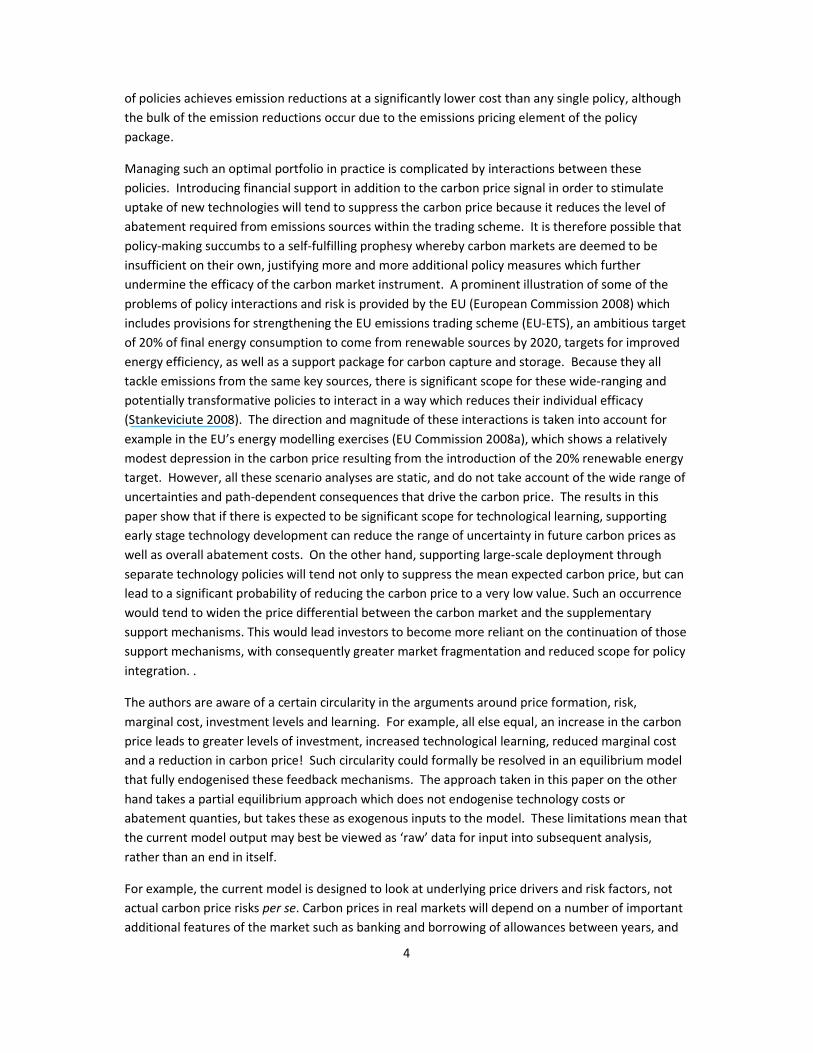
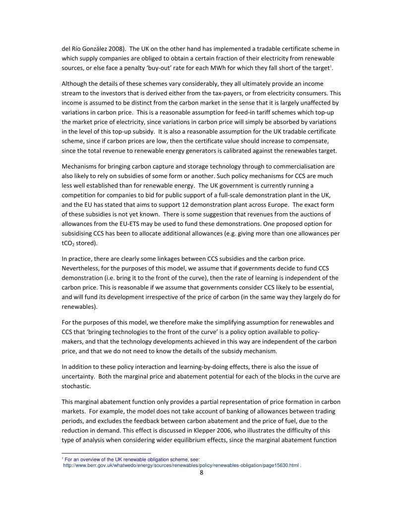
The apparently welfare-increasing solution is to bring forward the development phases D1 and D2 in

order to allow the mature technology tranche D3 to take its natural place in the ranking (as shown in

Figure 4). The cheaper technology D3 is now setting the carbon price at a lower level. However, this

may, or may not, be efficient. Notice that bringing more expensive technologies to the front of the

curve shifts the rest of the curve to the right, effectively displacing cheaper options A and B, and

suppressing the expected carbon price. The total cost of meeting the target (as measured by the

7

area under the curve) may increase or decrease as a result of this shift. The sign and magnitude of

the change in abatement cost depends on the additional cost of the initial technology tranches D1

and D2 relative to the benefits of bringing tranche D3 into the curve. This in turn depends on the rate

at which costs come down from one tranche to the next. In the classical representation of learning

curves, the cost of a technology comes down by a fixed percentage for every doubling of installed

capacity (IEA 2000). This representation of learning is similar in that the marginal cost of the second

tranche is less than the marginal cost of the first tranche (as a result of learning). In this case, the

amount of installed capacity required to achieve the reduction in cost is given by the width of bars

D1 and D2. Figure 4 therefore provides a graphical illustration of the result shown in Rosendahl 2004:

supporting technologies with high marginal costs (represented by the height of bars D1 and D2) can

be justified as long as the learning rate is fast enough (i.e. bars D1 and D2 are sufficiently narrow) that

the total cost of bringing the technology forward (i.e. the area of bars D1 and D2) is offset by the

gains from bringing D3 into the curve and displacing the more expensive technology C. Conversely, if

bars D1 and D2 turn out to be wider than expected (i.e. slower than expected learning), then the

policy measure will turn out to be more costly, and will suppress carbon prices to a greater extent

than expected.

AB

C

Abatement MtCO2Target

Marginal Cost

€/tCO2

Expected

PriceD3

D1

D2

Figure 4. Supporting early technology development allows the mature technology to enter the

abatement curve in its natural place

There are many different policy mechanisms available for supporting technology deployment

outside of the carbon market. Typically these comprise some form of subsidy targeted at a

particular technology or group of technologies with the aim of accelerating their entry into the

market. The example that is referred to in this paper is support for renewable electricity, for which

there are various types of policy instrument in operation in OECD countries; those that set a fixed

price per unit of electricity produced, those that mandate a set quantity of electricity to come from

renewable sources, and other types of direct subsidy. In the US, there are various subsidy

programmes at the Federal level. These include the production tax credit (PTC) and an investment

tax credit (ITC). In addition, 33 US States have enacted legislation to mandate electricity utilities to

provide a certain proportion of their electricity from renewable sources. In Europe, two main types

of scheme have been implemented; feed-in tariffs and tradable certificate schemes. Feed-in tariffs

typically either fix the price per kWh that renewable generators receive for their electricity, or they

provide a fixed top-up to the electricity price to bridge the gap between market prices and

renewable energy generation costs. In the EU, the two most prominent and successful feed-in tariff

systems have been implemented in Germany and Spain (e.g. for a review of the Spanish scheme, see

8

del Río González 2008). The UK on the other hand has implemented a tradable certificate scheme in

which supply companies are obliged to obtain a certain fraction of their electricity from renewable

sources, or else face a penalty ‘buy-out’ rate for each MWh for which they fall short of the target1.

Although the details of these schemes vary considerably, they all ultimately provide an income

stream to the investors that is derived either from the tax-payers, or from electricity consumers. This

income is assumed to be distinct from the carbon market in the sense that it is largely unaffected by

variations in carbon price. This is a reasonable assumption for feed-in tariff schemes which top-up

the market price of electricity, since variations in carbon price will simply be absorbed by variations

in the level of this top-up subsidy. It is also a reasonable assumption for the UK tradable certificate

scheme, since if carbon prices are low, then the certificate value should increase to compensate,

since the total revenue to renewable energy generators is calibrated against the renewables target.

Mechanisms for bringing carbon capture and storage technology through to commercialisation are

also likely to rely on subsidies of some form or another. Such policy mechanisms for CCS are much

less well established than for renewable energy. The UK government is currently running a

competition for companies to bid for public support of a full-scale demonstration plant in the UK,

and the EU has stated that aims to support 12 demonstration plant across Europe. The exact form

of these subsidies is not yet known. There is some suggestion that revenues from the auctions of

allowances from the EU-ETS may be used to fund these demonstrations. One proposed option for

subsidising CCS has been to allocate additional allowances (e.g. giving more than one allowances per

tCO2 stored).

In practice, there are clearly some linkages between CCS subsidies and the carbon price.

Nevertheless, for the purposes of this model, we assume that if governments decide to fund CCS

demonstration (i.e. bring it to the front of the curve), then the rate of learning is independent of the

carbon price. This is reasonable if we assume that governments consider CCS likely to be essential,

and will fund its development irrespective of the price of carbon (in the same way they largely do for

renewables).

For the purposes of this model, we therefore make the simplifying assumption for renewables and

CCS that ‘bringing technologies to the front of the curve’ is a policy option available to policy-

makers, and that the technology developments achieved in this way are independent of the carbon

price, and that we do not need to know the details of the subsidy mechanism.

In addition to these policy interaction and learning-by-doing effects, there is also the issue of

uncertainty. Both the marginal price and abatement potential for each of the blocks in the curve are

stochastic.

This marginal abatement function only provides a partial representation of price formation in carbon

markets. For example, the model does not take account of banking of allowances between trading

periods, and excludes the feedback between carbon abatement and the price of fuel, due to the

reduction in demand. This effect is discussed in Klepper 2006, who illustrates the difficulty of this

type of analysis when considering wider equilibrium effects, since the marginal abatement function

1 For an overview of the UK renewable obligation scheme, see: http://www.berr.gov.uk/whatwedo/energy/sources/renewables/policy/renewables-obligation/page15630.html .

9

is necessarily a simplified snap-shot of abatement opportunities under very particular assumptions.

Another feedback mechanism missing from this approach is the elasticity effect of increased carbon

prices (as implied by the marginal cost of meeting the abatement target) on energy demand. Both

of these effects are likely to reduce the (marginal and total) costs of meeting the abatement target

relative to the results presented in this paper. Inclusion of such feedbacks is left as a topic for further

research. Nevertheless, analysis of a stochastic abatement function with discriminatory policy

interventions can provide useful insights on the interaction of policies their evolutionary

implications.

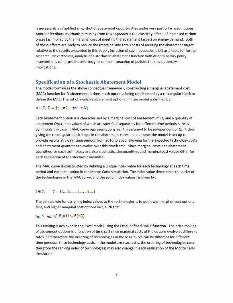
Specification of a Stochastic Abatement Model The model formalises the above conceptual framework, constructing a marginal abatement cost

(MAC) function for N abatement options, each option n being represented by a rectangular block to

define the MAC. The set of available abatement options T in the model is defined by:

Each abatement option n is characterised by a marginal cost of abatement P(n,t) and a quantity of

abatement Q(n,t) the values of which are specified separately for different time periods t. As is

commonly the case in MAC curve representations, P(n) is assumed to be independent of Q(n), thus

giving the rectangular block shape in the abatement curve. In our case, the model is set up to

provide results at 5-year time periods from 2010 to 2030, allowing for the expected technology costs

and abatement quantities to evolve over this timeframe. Since marginal costs and abatement

quantities for each technology are also stochastic, the quantities and marginal cost values differ for

each realisation of the stochastic variables.

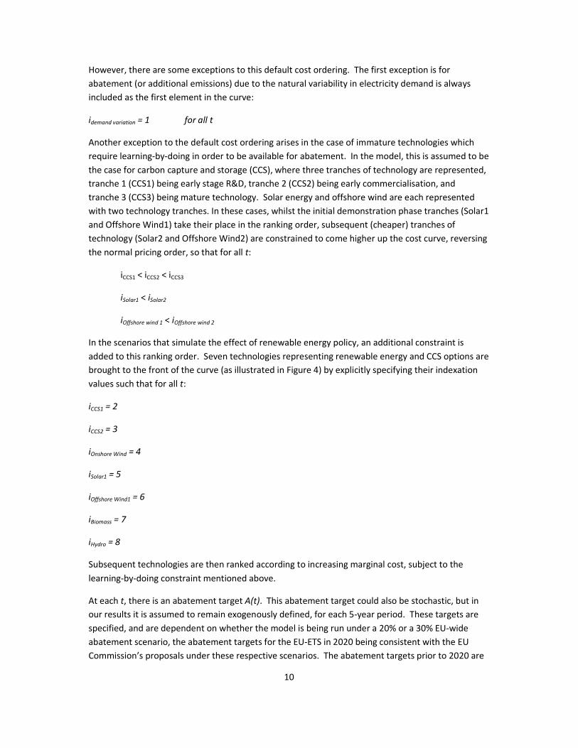
The MAC curve is constructed by defining a unique index value for each technology at each time

period and each realisation in the Monte Carlo simulation. The index value determines the order of

the technologies in the MAC curve, and the set of index values i is given by:

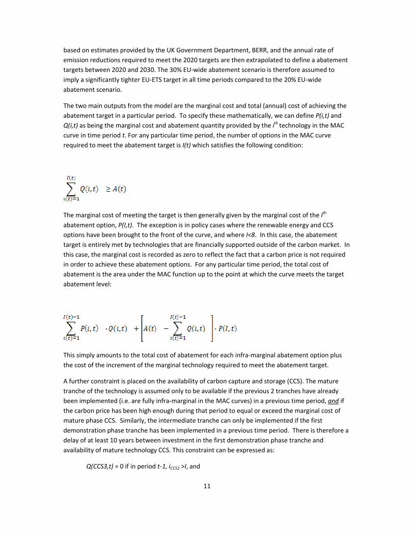
The default rule for assigning index values to the technologies is to put lower marginal cost options

first, and higher marginal cost options last, such that

This ranking is achieved in the Excel model using the Excel-defined RANK function. The price ranking

of abatement options is a function of time in(t) since marginal costs of the options evolve at different

rates, and therefore the ordering of technologies in the MAC curve can be different for different

time periods. Since technology costs in the model are stochastic, the ordering of technologies (and

therefore the ranking index of technologies) may also change in each realisation of the Monte Carlo

simulation.

10

However, there are some exceptions to this default cost ordering. The first exception is for

abatement (or additional emissions) due to the natural variability in electricity demand is always

included as the first element in the curve:

idemand variation = 1 for all t

Another exception to the default cost ordering arises in the case of immature technologies which

require learning-by-doing in order to be available for abatement. In the model, this is assumed to be

the case for carbon capture and storage (CCS), where three tranches of technology are represented,

tranche 1 (CCS1) being early stage R&D, tranche 2 (CCS2) being early commercialisation, and

tranche 3 (CCS3) being mature technology. Solar energy and offshore wind are each represented

with two technology tranches. In these cases, whilst the initial demonstration phase tranches (Solar1

and Offshore Wind1) take their place in the ranking order, subsequent (cheaper) tranches of

technology (Solar2 and Offshore Wind2) are constrained to come higher up the cost curve, reversing

the normal pricing order, so that for all t:

iCCS1 < iCCS2 < iCCS3

iSolar1 < iSolar2

iOffshore wind 1 < iOffshore wind 2

In the scenarios that simulate the effect of renewable energy policy, an additional constraint is

added to this ranking order. Seven technologies representing renewable energy and CCS options are

brought to the front of the curve (as illustrated in Figure 4) by explicitly specifying their indexation

values such that for all t:

iCCS1 = 2

iCCS2 = 3

iOnshore Wind = 4

iSolar1 = 5

iOffshore Wind1 = 6

iBiomass = 7

iHydro = 8

Subsequent technologies are then ranked according to increasing marginal cost, subject to the

learning-by-doing constraint mentioned above.

At each t, there is an abatement target A(t). This abatement target could also be stochastic, but in

our results it is assumed to remain exogenously defined, for each 5-year period. These targets are

specified, and are dependent on whether the model is being run under a 20% or a 30% EU-wide

abatement scenario, the abatement targets for the EU-ETS in 2020 being consistent with the EU

Commission’s proposals under these respective scenarios. The abatement targets prior to 2020 are

11

based on estimates provided by the UK Government Department, BERR, and the annual rate of

emission reductions required to meet the 2020 targets are then extrapolated to define a abatement

targets between 2020 and 2030. The 30% EU-wide abatement scenario is therefore assumed to

imply a significantly tighter EU-ETS target in all time periods compared to the 20% EU-wide

abatement scenario.

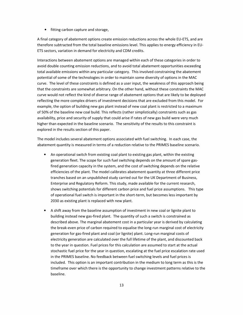
The two main outputs from the model are the marginal cost and total (annual) cost of achieving the

abatement target in a particular period. To specify these mathematically, we can define P(i,t) and

Q(i,t) as being the marginal cost and abatement quantity provided by the ith

technology in the MAC

curve in time period t. For any particular time period, the number of options in the MAC curve

required to meet the abatement target is I(t) which satisfies the following condition:

The marginal cost of meeting the target is then generally given by the marginal cost of the Ith

abatement option, P(I,t). The exception is in policy cases where the renewable energy and CCS

options have been brought to the front of the curve, and where I<8. In this case, the abatement

target is entirely met by technologies that are financially supported outside of the carbon market. In

this case, the marginal cost is recorded as zero to reflect the fact that a carbon price is not required

in order to achieve these abatement options. For any particular time period, the total cost of

abatement is the area under the MAC function up to the point at which the curve meets the target

abatement level:

This simply amounts to the total cost of abatement for each infra-marginal abatement option plus

the cost of the increment of the marginal technology required to meet the abatement target.

A further constraint is placed on the availability of carbon capture and storage (CCS). The mature

tranche of the technology is assumed only to be available if the previous 2 tranches have already

been implemented (i.e. are fully infra-marginal in the MAC curves) in a previous time period, and if

the carbon price has been high enough during that period to equal or exceed the marginal cost of

mature phase CCS. Similarly, the intermediate tranche can only be implemented if the first

demonstration phase tranche has been implemented in a previous time period. There is therefore a

delay of at least 10 years between investment in the first demonstration phase tranche and

availability of mature technology CCS. This constraint can be expressed as:

Q(CCS3,t) = 0 if in period t-1, iCCS2 >I, and

12

Q(CCS2,t) = 0 if in period t-1, iCCS1 >I,

A sensitivity case (labelled CCS+ in the results section) looks at the effect of accelerating CCS

development such that the mature phase of CCS is available 5 years (instead of 10 years) after the

initial demonstration phase. The assumption is still made that the carbon price needs to be

sufficiently high during these 5 years to stimulate commercialisation of the mature phase

technology.

The model includes 16 different abatement options, 5 of which are broken down into multiple price

tranches giving 22 elements in the curve altogether. For each abatement option and for each 5-year

period, the model specifies an expected (mean) value for marginal cost and quantity of abatement,

and then defines a separate stochastic process for each of these values. The stochastic processes

can be either entirely independent from each other, or can be correlated with other processes in the

model. Assumptions about technology cost and abatement potential are derived from the IEA’s

Energy Technology Perspectives (IEA 2008b) study, together with studies undertaken for the UK

government (Redpoint 2007, Poyry 2008).

The abatement options described in the model measure emission reductions relative to a business-

as-usual emissions baseline. The baseline used in this case was the baseline scenario for the EU-27

PRIMES model, as published in April 2008 (European Commission 2008a). The model takes account

of uncertainty in this baseline by including a contribution of uncertainty as the first element in the

cost curve running along the x-axis at zero cost. It can contribute either positively to the cost curve,

with the effect of pushing the whole MAC function to the right in situations where baseline

emissions are lower than expected making achievement of the target easier, or conversely can pull

the whole MAC function to the left representing a situation where baseline emissions are higher

than expected making achievement of the target more costly.

The PRIMES (op cit) emissions baseline was defined at a disaggregated level to provide emissions

levels for both existing plant and new build for each type of generation plant for each 5-year period

to 2030. This disaggregation is important because the different technology options abate emissions

from different parts of the baseline emissions. For example, re-ordering the dispatch (i.e. fuel

switching) from existing coal plant to existing gas plant only reduces emissions from existing coal

plant. As these plants retire over the period to 2030, the potential for abatement from this option

diminishes. On the other hand, renewables and nuclear abate emissions by changing the expected

mix of new plant, so the expected quantity of abatement E[Q]for these options increases over time

as the stock of new2 plant in the baseline increases over time. Some abatement options are fuel-

specific. For example, the following options abate emissions only from new coal build, and therefore

also increase in terms of abatement potential over time in line with expected new coal build in the

PRIMES baseline:

• building new gas plant instead of new coal plant

• building new integrated gasification and combined cycle (IGCC) plant instead of new coal

plant

2 ‘New’ plant here refers to plant build any time after the first year of the simulation.

13

• fitting carbon capture and storage,

A final category of abatement options create emission reductions across the whole EU-ETS, and are

therefore subtracted from the total baseline emissions level. This applies to energy efficiency in EU-

ETS sectors, variation in demand for electricity and CDM credits.

Interactions between abatement options are managed within each of these categories in order to

avoid double counting emission reductions, and to avoid total abatement opportunities exceeding

total available emissions within any particular category. This involved constraining the abatement

potential of some of the technologies in order to maintain some diversity of options in the MAC

curve. The level of these constraints is defined as a user input, the weakness of this approach being

that the constraints are somewhat arbitrary. On the other hand, without these constraints the MAC

curve would not reflect the kind of diverse range of abatement options that are likely to be deployed

reflecting the more complex drivers of investment decisions that are excluded from this model. For

example, the option of building new gas plant instead of new coal plant is restricted to a maximum

of 50% of the baseline new coal build. This reflects (rather simplistically) constraints such as gas

availability, price and security of supply that could arise if rates of new gas build were very much

higher than expected in the baseline scenario. The sensitivity of the results to this constraint is

explored in the results section of this paper.

The model includes several abatement options associated with fuel switching. In each case, the

abatement quantity is measured in terms of a reduction relative to the PRIMES baseline scenario.

• An operational switch from existing coal plant to existing gas plant, within the existing

generation fleet. The scope for such fuel switching depends on the amount of spare gas-

fired generation capacity in the system, and the cost of switching depends on the relative

efficiencies of the plant. The model calibrates abatement quantity at three different price

tranches based on an unpublished study carried out for the UK Department of Business,

Enterprise and Regulatory Reform. This study, made available for the current research,

shows switching potentials for different carbon price and fuel price assumptions. This type

of operational fuel switch is important in the short-term, but becomes less important by

2030 as existing plant is replaced with new plant.

• A shift away from the baseline assumption of investment in new coal or lignite plant to

building instead new gas-fired plant. The quantity of such a switch is constrained as

described above. The marginal abatement cost in a particular year is derived by calculating

the break-even price of carbon required to equalise the long-run marginal cost of electricity

generation for gas-fired plant and coal (or lignite) plant. Long-run marginal costs of

electricity generation are calculated over the full lifetime of the plant, and discounted back

to the year in question. Fuel prices for this calculation are assumed to start at the actual

stochastic fuel price for the year in question, escalating at the fuel price escalation rate used

in the PRIMES baseline. No feedback between fuel switching levels and fuel prices is

included. This option is an important contribution in the medium to long term as this is the

timeframe over which there is the opportunity to change investment patterns relative to the

baseline.

14

• An early replacement of existing coal plant with new gas plant. This option calculates the

break-even price of carbon required to equalise the short-run marginal cost of electricity

generation from coal plant with the long-run marginal cost of generation from gas plant.

This option is only relevant in the short term, and tends to be very expensive, so does not

play a significant role in the results.

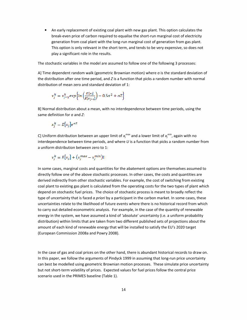
The stochastic variables in the model are assumed to follow one of the following 3 processes:

A] Time dependent random walk (geometric Brownian motion) where σ is the standard deviation of

the distribution after one time period, and Z is a function that picks a random number with normal

distribution of mean zero and standard deviation of 1:

B] Normal distribution about a mean, with no interdependence between time periods, using the

same definition for σ and Z:

C] Uniform distribution between an upper limit of xjmax

and a lower limit of xjmin

, again with no

interdependence between time periods, and where U is a function that picks a random number from

a uniform distribution between zero to 1:

In some cases, marginal costs and quantities for the abatement options are themselves assumed to

directly follow one of the above stochastic processes. In other cases, the costs and quantities are

derived indirectly from other stochastic variables. For example, the cost of switching from existing

coal plant to existing gas plant is calculated from the operating costs for the two types of plant which

depend on stochastic fuel prices. The choice of stochastic process is meant to broadly reflect the

type of uncertainty that is faced a priori by a participant in the carbon market. In some cases, these

uncertainties relate to the likelihood of future events where there is no historical record from which

to carry out detailed econometric analysis. For example, in the case of the quantity of renewable

energy in the system, we have assumed a kind of ‘absolute’ uncertainty (i.e. a uniform probability

distribution) within limits that are taken from two different published sets of projections about the

amount of each kind of renewable energy that will be installed to satisfy the EU’s 2020 target

(European Commission 2008a and Powry 2008).

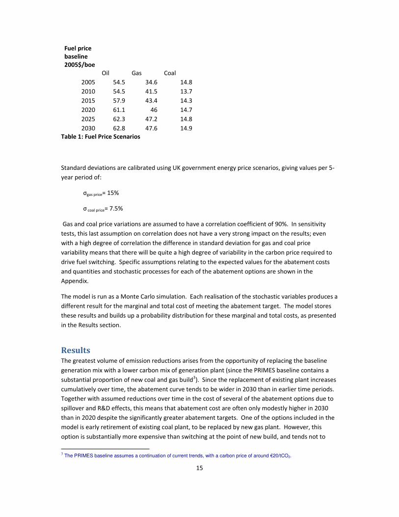
In the case of gas and coal prices on the other hand, there is abundant historical records to draw on.

In this paper, we follow the arguments of Pindyck 1999 in assuming that long-run price uncertainty

can best be modelled using geometric Brownian motion processes. These simulate price uncertainty

but not short-term volatility of prices. Expected values for fuel prices follow the central price

scenario used in the PRIMES baseline (Table 1).

15

Fuel price

baseline

2005$/boe

Oil Gas Coal

2005 54.5 34.6 14.8

2010 54.5 41.5 13.7

2015 57.9 43.4 14.3

2020 61.1 46 14.7

2025 62.3 47.2 14.8

2030 62.8 47.6 14.9

Table 1: Fuel Price Scenarios

Standard deviations are calibrated using UK government energy price scenarios, giving values per 5-

year period of:

σgas price= 15%

σ coal price= 7.5%

Gas and coal price variations are assumed to have a correlation coefficient of 90%. In sensitivity

tests, this last assumption on correlation does not have a very strong impact on the results; even

with a high degree of correlation the difference in standard deviation for gas and coal price

variability means that there will be quite a high degree of variability in the carbon price required to

drive fuel switching. Specific assumptions relating to the expected values for the abatement costs

and quantities and stochastic processes for each of the abatement options are shown in the

Appendix.

The model is run as a Monte Carlo simulation. Each realisation of the stochastic variables produces a

different result for the marginal and total cost of meeting the abatement target. The model stores

these results and builds up a probability distribution for these marginal and total costs, as presented

in the Results section.

Results The greatest volume of emission reductions arises from the opportunity of replacing the baseline

generation mix with a lower carbon mix of generation plant (since the PRIMES baseline contains a

substantial proportion of new coal and gas build3). Since the replacement of existing plant increases

cumulatively over time, the abatement curve tends to be wider in 2030 than in earlier time periods.

Together with assumed reductions over time in the cost of several of the abatement options due to

spillover and R&D effects, this means that abatement cost are often only modestly higher in 2030

than in 2020 despite the significantly greater abatement targets. One of the options included in the

model is early retirement of existing coal plant, to be replaced by new gas plant. However, this

option is substantially more expensive than switching at the point of new build, and tends not to

3 The PRIMES baseline assumes a continuation of current trends, with a carbon price of around €20/tCO2.

16

contribute much to the abatement curves. The most significant abatement options in the early time

periods tend to be fuel switching to gas from existing coal plant, and CDM credits, whilst the later

time period includes a wider range of abatement options as described in the Appendix.

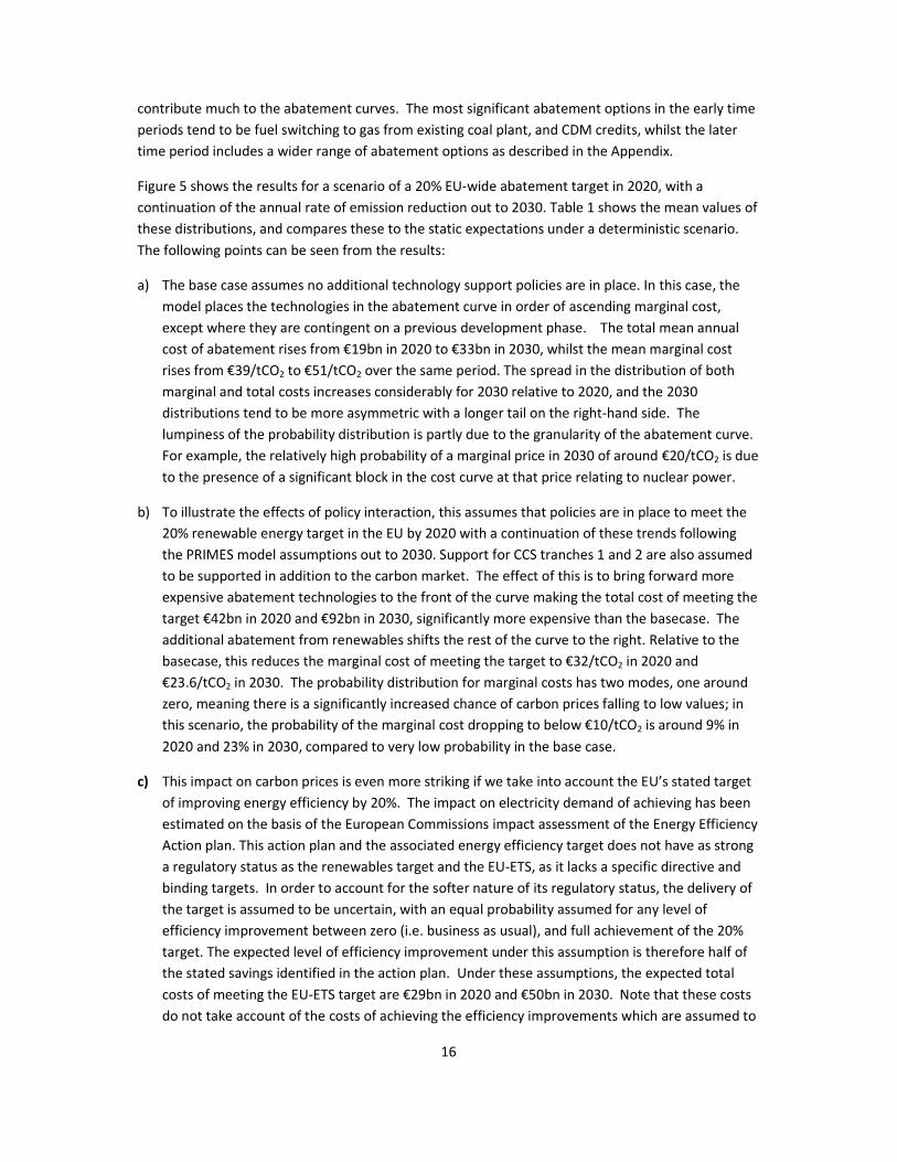
Figure 5 shows the results for a scenario of a 20% EU-wide abatement target in 2020, with a

continuation of the annual rate of emission reduction out to 2030. Table 1 shows the mean values of

these distributions, and compares these to the static expectations under a deterministic scenario.

The following points can be seen from the results:

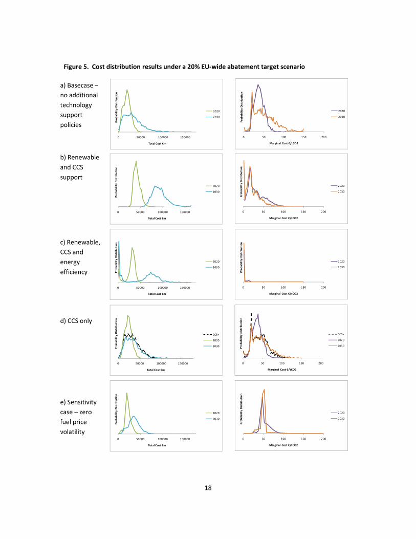
a) The base case assumes no additional technology support policies are in place. In this case, the

model places the technologies in the abatement curve in order of ascending marginal cost,

except where they are contingent on a previous development phase. The total mean annual

cost of abatement rises from €19bn in 2020 to €33bn in 2030, whilst the mean marginal cost

rises from €39/tCO2 to €51/tCO2 over the same period. The spread in the distribution of both

marginal and total costs increases considerably for 2030 relative to 2020, and the 2030

distributions tend to be more asymmetric with a longer tail on the right-hand side. The

lumpiness of the probability distribution is partly due to the granularity of the abatement curve.

For example, the relatively high probability of a marginal price in 2030 of around €20/tCO2 is due

to the presence of a significant block in the cost curve at that price relating to nuclear power.

b) To illustrate the effects of policy interaction, this assumes that policies are in place to meet the

20% renewable energy target in the EU by 2020 with a continuation of these trends following

the PRIMES model assumptions out to 2030. Support for CCS tranches 1 and 2 are also assumed

to be supported in addition to the carbon market. The effect of this is to bring forward more

expensive abatement technologies to the front of the curve making the total cost of meeting the

target €42bn in 2020 and €92bn in 2030, significantly more expensive than the basecase. The

additional abatement from renewables shifts the rest of the curve to the right. Relative to the

basecase, this reduces the marginal cost of meeting the target to €32/tCO2 in 2020 and

€23.6/tCO2 in 2030. The probability distribution for marginal costs has two modes, one around

zero, meaning there is a significantly increased chance of carbon prices falling to low values; in

this scenario, the probability of the marginal cost dropping to below €10/tCO2 is around 9% in

2020 and 23% in 2030, compared to very low probability in the base case.

c) This impact on carbon prices is even more striking if we take into account the EU’s stated target

of improving energy efficiency by 20%. The impact on electricity demand of achieving has been

estimated on the basis of the European Commissions impact assessment of the Energy Efficiency

Action plan. This action plan and the associated energy efficiency target does not have as strong

a regulatory status as the renewables target and the EU-ETS, as it lacks a specific directive and

binding targets. In order to account for the softer nature of its regulatory status, the delivery of

the target is assumed to be uncertain, with an equal probability assumed for any level of

efficiency improvement between zero (i.e. business as usual), and full achievement of the 20%

target. The expected level of efficiency improvement under this assumption is therefore half of

the stated savings identified in the action plan. Under these assumptions, the expected total

costs of meeting the EU-ETS target are €29bn in 2020 and €50bn in 2030. Note that these costs

do not take account of the costs of achieving the efficiency improvements which are assumed to

17

occur outside of the EU-ETS. It is interesting to note that the stochastic mean total cost is

significantly lower than the deterministic expected value. This is because under a deterministic

scenario the abatement target is almost entirely met by energy efficiency and renewable energy

measures. Under the stochastic scenario, costs are lower because in cases where abatement

requirement is greater than expected, low cost measures are available which do not add much

to the total cost of abatement, whereas when abatement requirement is less than expected, the

amount of renewables required to meet the abatement target is lower, reducing the total costs

significantly. The effect on marginal costs of including energy efficiency is dramatic, reducing the

expected values to only €3.5/tCO2 in 2020 and €1.5/tCO2 in 2030. The total costs are also

strongly affected, resulting in a probability distribution with two modes, one around zero. This

suggests that in some states of the world (corresponding to low economic growth, low energy

prices and yet still achieving the 20% efficiency target), the greenhouse gas target would be met

at close to zero cost – i.e. it would be met under business as usual without any additional

abatement required.

d) When only the first and second tranches of CCS are brought to the front of the MAC curve, the

effect is to slightly increase the total costs of meeting the target, and reduce the marginal costs.

There is no significant financial gain to supporting CCS under this scenario since the mature

phase of CCS is not required to meet the target in 2030. Similar results are shown for 2030 for

the additional sensitivity case is illustrated with the label “CCS+” to denote an accelerated

technology development scenario where the mature phase of CCS is available only 5 years after

the initial demonstration phase (i.e. assuming CCS1 is implemented in 2015, CCS3 is available

from 2020 onwards). Again, in the 20% abatement scenario, the availability of CCS does not

significantly alter the results compared to the basecase. This contrasts with the case of a 30%

EU-wide abatement target where CCS availability affects the results strongly, as described

below.

e) Case e) looks at the sensitivity of the cost results to fuel price uncertainty. The results show that

removing fuel price uncertainty from the model produces a major reduction in the uncertainty in

marginal cost. This is because under deterministic fuel prices and a 20% EU-wide abatement

scenario, fuel switching from coal to gas is very often the marginal abatement option, leading to

a much narrower distribution in marginal cost. It should be noted that the actual effect of

removing uncertainty in fuel price would have broader consequences than those indicated in

this analysis since in reality it would change the economics of individual elements of the cost-

curve through changes in the risk profile of investments, an effect that is not modelled here.

Nevertheless, this sensitivity analysis is a useful indication that fuel price uncertainty is a major

source of carbon price uncertainty under this scenario. This contrasts with results in Figure 6e

which indicate a different set of price drivers under a 30% abatement scenario.

18

Figure 5. Cost distribution results under a 20% EU-wide abatement target scenario

0 50000 100000 150000

Pro

ba

bil

ity

Dis

trib

uti

on

Total Cost €m

2020

2030

0 50 100 150 200

Pro

ba

bili

ty D

istr

ibu

tio

n

Marginal Cost €/tCO2

2020

2030

0 50000 100000 150000

Pro

bab

ilit

y D

istr

ibu

tio

n

Total Cost €m

2020

2030

0 50 100 150 200

Pro

bab

ilit

y D

istr

ibu

tio

n

Marginal Cost €/tCO2

2020

2030

0 50000 100000 150000

Pro

ba

bil

ity

Dis

trib

uti

on

Total Cost €m

2020

2030

0 50 100 150 200

Pro

ba

bil

ity

Dis

trib

uti

on

Marginal Cost €/tCO2

2020

2030

0 50000 100000 150000

Pro

ba

bil

ity

Dis

trib

uti

on

Total Cost €m

2020

2030

0 50 100 150 200

Pro

ba

bili

ty D

istr

ibu

tio

n

Marginal Cost €/tCO2

2020

2030

0 50000 100000 150000

Pro

bab

ilit

y D

istr

ibu

tio

n

Total Cost €m

CCS+

2020

2030

0 50 100 150 200

Pro

ba

bili

ty D

istr

ibu

tio

n

Marginal Cost €/tCO2

CCS+

2020

2030

a) Basecase –

no additional

technology

support

policies

b) Renewable

and CCS

support

c) Renewable,

CCS and

energy

efficiency

d) CCS only

e) Sensitivity

case – zero

fuel price

volatility

19

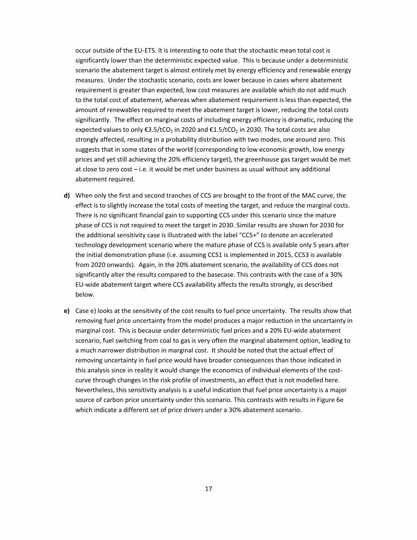
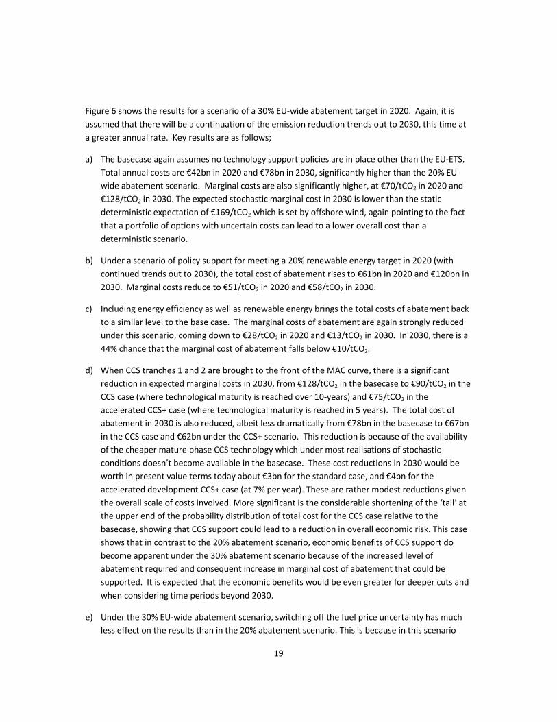
Figure 6 shows the results for a scenario of a 30% EU-wide abatement target in 2020. Again, it is

assumed that there will be a continuation of the emission reduction trends out to 2030, this time at

a greater annual rate. Key results are as follows;

a) The basecase again assumes no technology support policies are in place other than the EU-ETS.

Total annual costs are €42bn in 2020 and €78bn in 2030, significantly higher than the 20% EU-

wide abatement scenario. Marginal costs are also significantly higher, at €70/tCO2 in 2020 and

€128/tCO2 in 2030. The expected stochastic marginal cost in 2030 is lower than the static

deterministic expectation of €169/tCO2 which is set by offshore wind, again pointing to the fact

that a portfolio of options with uncertain costs can lead to a lower overall cost than a

deterministic scenario.

b) Under a scenario of policy support for meeting a 20% renewable energy target in 2020 (with

continued trends out to 2030), the total cost of abatement rises to €61bn in 2020 and €120bn in

2030. Marginal costs reduce to €51/tCO2 in 2020 and €58/tCO2 in 2030.

c) Including energy efficiency as well as renewable energy brings the total costs of abatement back

to a similar level to the base case. The marginal costs of abatement are again strongly reduced

under this scenario, coming down to €28/tCO2 in 2020 and €13/tCO2 in 2030. In 2030, there is a

44% chance that the marginal cost of abatement falls below €10/tCO2.

d) When CCS tranches 1 and 2 are brought to the front of the MAC curve, there is a significant

reduction in expected marginal costs in 2030, from €128/tCO2 in the basecase to €90/tCO2 in the

CCS case (where technological maturity is reached over 10-years) and €75/tCO2 in the

accelerated CCS+ case (where technological maturity is reached in 5 years). The total cost of

abatement in 2030 is also reduced, albeit less dramatically from €78bn in the basecase to €67bn

in the CCS case and €62bn under the CCS+ scenario. This reduction is because of the availability

of the cheaper mature phase CCS technology which under most realisations of stochastic

conditions doesn’t become available in the basecase. These cost reductions in 2030 would be

worth in present value terms today about €3bn for the standard case, and €4bn for the

accelerated development CCS+ case (at 7% per year). These are rather modest reductions given

the overall scale of costs involved. More significant is the considerable shortening of the ‘tail’ at

the upper end of the probability distribution of total cost for the CCS case relative to the

basecase, showing that CCS support could lead to a reduction in overall economic risk. This case

shows that in contrast to the 20% abatement scenario, economic benefits of CCS support do

become apparent under the 30% abatement scenario because of the increased level of

abatement required and consequent increase in marginal cost of abatement that could be

supported. It is expected that the economic benefits would be even greater for deeper cuts and

when considering time periods beyond 2030.

e) Under the 30% EU-wide abatement scenario, switching off the fuel price uncertainty has much

less effect on the results than in the 20% abatement scenario. This is because in this scenario

20

fuel switching is almost always inframarginal. Reduced variability in fuel prices therefore reduces

the variability of total abatement costs, but makes very little difference to the variability in

marginal cost. This is significant from the point of view of understanding carbon-price risks,

since it illustrates that the drivers of carbon price variability could be significantly different under

a 30% abatement scenario compared to a 20% abatement scenario.

21

Figure 6. Cost distribution results under a 30% EU-wide abatement target scenario

0 50000 100000 150000

Pro

ba

bil

ity

Dis

trib

uti

on

Total Cost €m

2020

2030

0 50 100 150 200

Pro

bab

ility

Dis

trib

uti

on

Marginal Cost €/tCO2

2020

2030

0 50000 100000 150000

Pro

bab

ility

Dis

trib

uti

on

Total Cost €m

2020

2030

0 50 100 150 200

Pro

ba

bil

ity

Dis

trib

uti

on

Marginal Cost €/tCO2

2020

2030

0 50000 100000 150000

Pro

ba

bil

ity

Dis

trib

uti

on

Total Cost €m

2020

2030

0 50 100 150 200

Pro

bab

ility

Dis

trib

uti

on

Marginal Cost €/tCO2

2020

2030

0 50000 100000 150000

Pro

ba

bil

ity

Dis

trib

uti

on

Total Cost €m

2020

2030

0 50 100 150 200

Pro

ba

bili

ty D

istr

ibu

tio

n

Marginal Cost €/tCO2

2020

2030

0 50 100 150 200

Pro

bab

ility

Dis

trib

uti

on

Marginal Cost €/tCO2

CCS+

2020

2030

0 50000 100000 150000

Pro

bab

ility

Dis

trib

uti

on

Total Cost €m

CCS+

2020

2030

a) Basecase –

no additional

technology

support

policies

b) Renewable

and CCS

support

c) Renewable,

CCS and

energy

efficiency

d) CCS only

e) Sensitivity

case – zero

fuel price

volatility

22

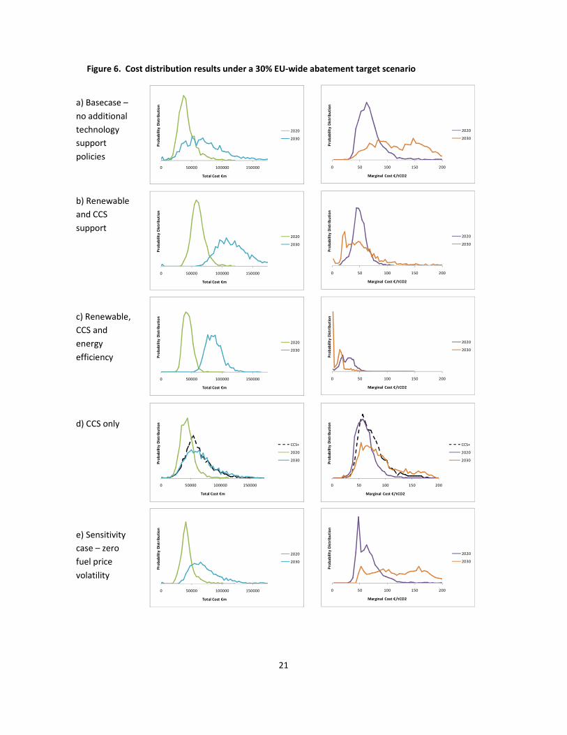
Table 1. Expected values and distributions

Case

Marginal cost results €/tCO2 Total cost €m Deterministic

Marginal Cost

Deterministic

Total Cost

mean

Prob

<€10

Prob. outside

±30% range Mean

Total outside

±30% range €/tCO2 €m

5a) 20% basecase 2020 39.1 0.1% 41% 19451 72% 46 14223

2030 50.6 1.5% 63% 32520 71% 50 21860

5b) 20%+RE+CCS 2020 32.0 9.1% 73% 42260 15% 29 38331

2030 23.6 22.6% 80% 92450 10% 33 86408

5c) 20%+RE+CCS+EE 2020 3.5 88.0% 100% 28881 36% 13 33448

2030 1.5 98.8% #N/A 49611 92% 0 81269

5d) 20% +CCS 2020 36.6 0.5% 42% 23718 59% 40 18556

2030 45.0 3.4% 63% 33861 60% 50 24459

Accelerated CCS+ 2030 42.35 2% 62% 32772 70%

5e) 20% deterministic fuel price 2020 53.2 0.1% 20% 21816 35% 46 14223

2030 50.5 0.0% 15% 35310 46% 50 21860

6a) 30% basecase 2020 69.8 0.0% 35% 42156 30% 60 34587

2030 127.7 0.1% 54% 78596 57% 169 50795

6b) 30% +RE CCS 2020 51.0 0.1% 25% 60926 11% 50 55283

2030 58.1 3.5% 64% 120050 20% 50 102417

6c) 30% +RE CCS EE 2020 27.5 6.2% 66% 43508 10% 46 44497

2030 13.3 44.3% 79% 86537 8% 33 86716

6d) 30% +CCS 2020 62.4 0.0% 29% 44248 27% 60 37901

2030 90.0 0.0% 51% 67374 43% 54 45805

Accelerated CCS+ 2030 74.5 0.0% 32% 62256.3 36% 54 45805

6e) 30% deterministic fuel price 2020 66.5 0.0% 30% 42793 23% 60 34587

2030 126.7 0.0% 55% 76962 39% 169 50795

23

Sensitivity Analyses for the Base Case As for all models, the results are dependent on the assumptions, so a number of model runs were

carried out to try to determine some of the key sensitivities, in addition to the test of sensitivity to

fuel price variability described in the results above. The parameters tested for sensitivity include;

1. Variability in electricity demand. In this sensitivity test, electricity demand was set to its

average value, with no stochastic variation in order to determine the impact on overall cost

variability. This sensitivity test shows that the role of variability in electricity demand is fairly

modest. As expected, the mean values for total and marginal cost are unaffected by

removal of the symmetrical variation in demand. The spread in total cost is reduced by

about 15%, and the range for marginal cost is reduced by about 10% relative to the base

case.

2. Variability of the CDM price. In the base case scenario, it is assumed that the price of CDM

credits would depend on whether a 20% or a 30% EU-wide abatement scenario is being

considered. The logic of this is that switch between a 20% to a 30% EU-wide abatement

target implies a shift towards an international climate policy deal reached under the

UNFCCC implying concerted global abatement effort and a significant increase in demand for

CDM (or some other equivalent international) credits. In the base case 20% abatement

scenario, CDM credit prices vary between €6-19/tCO2 in 2020, and between €34-134/tCO2 in

2030. In the base case 30% EU-wide abatement scenario, CDM prices range from €19-

80/tCO2 in 2020, and €134-210/tCO2 in 2030. These ranges of prices are taken from results

of the GLOCAF model run by the UK Department of Energy and Climate Change. However, a

sensitivity variation to this assumption is that the choice between a 20% or 30% EU-wide

abatement target does not have such a strong causal link to the global demand for and price

of CDM credits. The sensitivity case therefore allows CDM prices to span the full range of

variability shown in the GLOCAF results (i.e. €6-80/tCO2 in 2020, and between €34-210/tCO2

in 2030). This has the effect of increasing the total abatement costs under the 20%

abatement scenario (from €19bn to €31bn in 2020 and from €33bn to €56bn in 2030)

relative to the base case. Although CDM price under the GLOCAF scenario is higher than the

marginal abatement cost under deterministic conditions, under stochastic conditions, CDM

becomes inframarginal less often in the sensitivity case, raising the abatement cost

compared to the base case. Under the 30% abatement scenario, costs are reduced because

of the cheaper average price of CDM credits in the sensitivity case compared to the 30%

abatement base case. However, the reduction is quite small, with total costs only about

€2bn lower than the base case.

3. Remove constraints on building new gas-fired generation. One of the limitations of a cost-

curve model is that it simply chooses the cheapest available option, without taking account

of other indirect benefits associated with diversity. In the base case, a fixed constraint is

included in the model so that no more than 50% of the expected new build of coal plant up

to the period 2030 can be replaced with new gas plant. To test the sensitivity of the results

24

to this assumption, a run was made removing this constraint such that up to 100% of new

coal plant could be replaced by new gas plant if it is cost-effective to do so. This case

illustrates an interesting effect associated with technology interactions. Removing the

constraint on building of new gas-fired plant instead of new coal-fired plant reduces the

expected marginal cost of reaching the abatement target by about 10%. This is not because

a move to gas is expected to be cheaper than the alternatives (it is actually the marginal

abatement option under expected prices in 2020 under the base case assumptions), but

because without the constraint, this option is more likely to be the marginal technology

under realisations of the model when the gas price is low implying a lower marginal cost of

abatement. However, this benefit does not translate into a reduction in total costs. The

mean total cost of abatement is actually higher in Sensitivity Case 4 than under the Base

Case. This is because under the model assumptions, an increase in new gas build competes

with other new build options, notably IGCC plant, which is cost-effective under 2030 fuel

price and technology cost assumptions in the model. Squeezing out IGCC increases total

abatement costs by about 5-10% in this sensitivity case. Clearly, these results on total costs

are dependent on model assumptions on how different technology options compete, and a

more comprehensive capacity expansion model would probably be needed to investigate

such effects in more detail.

Conclusions Carbon markets are subject to a number of risks, not least of which is the level of the cap. For

example, the EU is committed to a unilateral GHG abatement target of 20% in 2020 relative to 1990,

increasing to 30% abatement if other major economies were to take on similar commitments within

an international climate agreement (European Council 2007). Achievement of 30% EU-wide

abatement would require a significant ramp-up of abatement effort, including more stringent EU-

ETS caps, and increased levels of international trading (European Commission 2008). At the same

time, ambitious targets for renewable energy in the EU will themselves achieve considerable

emission reductions, and therefore have important interactions with the carbon market. Previous

research on the price behaviour of the EU-ETS has focused on the role of fuel switching between

coal and gas, as well as the price profile of international credits, the two key short-term abatement

measures available to the market. However, when looking over the longer term, future risk drivers

may be quite different from the past. For example, the capacity for fuel switching is largely an

inherited feature of the electricity system which may not persist as the electricity system evolves

over time in the presence of a carbon price. This paper shows that the marginal technology driving

carbon prices in the future is highly dependent on the abatement target and additional technology

support mechanisms, which implies that climate policy not only has a direct effect on the expected

price, but also strongly affects the risk characteristics of the carbon market.

The model used in this paper is based on a stochastic marginal abatement cost (MAC) function. This

structure allows technology cost uncertainty to be modelled in detail. Each abatement option in the

MAC has separate assumptions about uncertainty in costs and abatement potential used to drive the

stochastic processes. The model also includes uncertainty in the baseline emissions, and uncertainty

25

in fuel prices. This model allows the expected cost of each abatement option to evolve in a number

of ways. Firstly, expected costs can come down over time (as a result of technological learning

through spill-overs or R&D). Secondly, the cost of some abatement options depends on direct

experience of deploying that technology, so that early demonstration plant may be more expensive,

and subsequent abatement from that technology is cheaper (i.e. learning-by-doing). Thirdly, some

abatement options become more expensive over time due to assumed resource constraints.

The model has been implemented in the context of the 2008 EU climate policy package. Key

features of this include: a unilateral EU-wide commitment to achieving 20% abatement in

greenhouse gas emissions to be increased to a 30% abatement target if other major economies take

similar commitments; a directive mandating 20% of the final energy demand in the EU to come from

renewable energy sources; a policy goal of improving energy efficiency by 20%; measures to support

early demonstration of carbon capture and storage technology; and strengthening of the EU

emissions trading scheme.

The model illustrates the following key results and conclusions:

• Supporting large-scale deployment of renewable energy to meet the EU policy of achieving

20% renewable energy supply reduces the abatement effort required in the EU-ETS. This

significantly reduces the expected marginal cost of abatement, increases the probability of

the carbon price dropping close to zero, whilst significantly increasing the overall cost of

achieving the abatement target. Introduction of additional energy efficiency measures

whilst keeping the EU-ETS target unchanged results in a high probability of a very low carbon

price.

• The case for providing support for technology development over and above the carbon price

is illustrated by the case of supporting an initial tranche of more expensive demonstration

plant for carbon capture and storage (CCS). This can reduce overall abatement costs because

it allows the cheaper mature phase of the technology to be introduced at a later date. The

total cost reductions are rather modest in 2030, and are only realised in the more stringent

abatement scenario of a 30% EU-wide abatement target, since the technology is not

required before 2030 under the 20% abatement scenario. The cost reductions beyond 2030

are expected to be greater. They are also sensitive to the assumed rate of technological

development; the sooner the cheaper mature phase of the CCS technology becomes

available, the greater the cost reductions in 2030. The results indicate a considerable

reduction in marginal abatement cost when CCS is made available through early

demonstration of the technology. This result illustrates that it will be important to support

technology development in a timely manner depending on the particular technology

development pathway in question, and depending on the rate at which convergence

between the cost of technology support and carbon prices are expected to occur.

• The model indicates that having a portfolio of different abatement options available can

help to reduce the overall abatement cost uncertainty, even when the costs of individual

abatement options are highly uncertain. This indicates that making available a reasonably

wide range of options from which cost-effective solutions can be chosen could be a useful

risk-reduction strategy, and reinforces the benefits of early-stage technology development.

26

• Sensitivity analyses indicate that the key drivers of marginal cost (and therefore price risk) in

a carbon market depend on what the marginal abatement options are expected to be. So

far in the EU-ETS, the carbon price has been driven strongly by gas price variability because

fuel switching from coal to gas in surplus capacity has been the marginal abatement option.

Under a 20% EU-wide abatement scenario, gas price variability continues to be a strong

driver of variability in the marginal abatement cost. Under a more ambitious 30% EU-wide

abatement scenario, the choice between coal and gas plant is rarely the marginal abatement

option, so fuel price variability has little effect on marginal abatement cost variability. This

result indicates that climate policy affects not only the expected price, but also the risk

characteristics of the carbon market.

• The range of abatement costs in 2030 is considerably wider than in 2020 because of the

accumulation of uncertainty over the longer time period for each of the stochastic variables

in the model. The lower bounds of the probability distribution of marginal cost tend to be

similar for 2020 and 2030, but there tends to be a longer tail towards higher marginal costs

in 2030. The fact that uncertainties can accumulate over time needs to be taken into

account when considering the length of allocation periods. Previous work by the authors

(Blyth et al 2007) indicated that longer allocation periods could reduce the policy risk

element of carbon prices. This conclusion needs to be weighed against the importance of

other risk factors driving the carbon price, and the potential need for policy to be adaptive

to changing circumstances. Further work to enumerate the balance between these various

risk factors is required.

• The expected values of marginal and total costs derived from the stochastic model can

deviate quite strongly from the deterministic values derived from the static marginal cost

curve constructed from the expected marginal costs of each technology. These deviations

occur because of the non-linear nature of the cost curve, and illustrate the additional

insights that can be gained from taking a stochastic rather than a static analytical approach.

As with any model-based analysis, our representation is not a complete model of carbon pricing,

since it excludes banking of permits as well some potentially important feedback mechanisms

between carbon abatement, fuel prices and electricity demand. Nevertheless, the results indicate

that supporting technology development can potentially disrupt market price signals. Policy

formation needs to take account of these effects, and can be informed by the kind of extensive

stochastic modelling of path-dependent abatement interactions presented in this paper.

27

APPENDIX. Base Case Assumptions for abatement options

Technology Expected

Marginal Cost

€/tCO2

Expected

Abatement

Quantity MtCO2

Description of Stochastic Process. Values of σ relate to standard deviation per 5-

year period.

2020 2030 2020 2030 Marginal Cost Quantity

Variation in power demand,

translated into emissions

uncertainty assuming baseline

average emissions factor.

0 0 0 0 Not stochastic Geometric Brownian motion process for total

power generation, σ=4.5%

Fuel Switching from existing coal

to exising gas (Tranche 1)

20 20 0 0 Not stochastic. Results are post-

processed to provide a smooth

probability distribution between

the three price tranches.

The quantity of abatement available at each

price tranche depends on the relative price of

gas and coal and the economics of switching.

These abatement potentials are calibrated

against model results from BERR showing the

level of fuel switching abatement that occurs

under different price scenarios.

Fuel Switching from existing coal

to exising gas (Tranche 2)

40 40 260 210

Fuel Switching from existing coal

to exising gas (Tranche 3)

60 60 400 325

Build new gas instead of new

coal plant. Abatement costs

based on the carbon price

required to equalise the short-

run marginal costs generation

between the two technologies.

46 50 162 307 All elements other than fuel prices

in the marginal cost calculation

(capital, O&M, efficiency, load

factor etc.) are assumed to be

deterministic.

Geometric Brownian motion σ= 10%

Build new gas instead of new

lignite plant, calculated as

above.

29 33 146 241 Based on short-run marginal costs,

with stochastic fuel prices.

Geometric Brownian motion σ= 10%

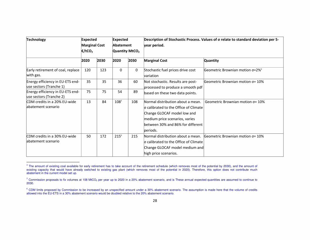
28

Technology Expected

Marginal Cost

€/tCO2

Expected

Abatement

Quantity MtCO2

Description of Stochastic Process. Values of σ relate to standard deviation per 5-

year period.

2020 2030 2020 2030 Marginal Cost Quantity

Early retirement of coal, replace

with gas.

120 123 0 0 Stochastic fuel prices drive cost

variation

Geometric Brownian motion σ=2%4

Energy efficiency in EU-ETS end-

use sectors (Tranche 1)

35 35 36 60 Not stochastic. Results are post-

processed to produce a smooth pdf

based on these two data points.

Geometric Brownian motion σ= 10%

Energy efficiency in EU-ETS end-

use sectors (Tranche 2)

75 75 54 89

CDM credits in a 20% EU-wide

abatement scenario

13

84

1085 108 Normal distribution about a mean.

σ calibrated to the Office of Climate

Change GLOCAF model low and

medium price scenarios, varies

between 30% and 86% for different

periods.

Geometric Brownian motion σ= 10%

CDM credits in a 30% EU-wide

abatement scenario

50 172 2156 215 Normal distribution about a mean.

σ calibrated to the Office of Climate

Change GLOCAF model medium and

high price scenarios.

Geometric Brownian motion σ= 10%

4 The amount of existing coal available for early retirement has to take account of the retirement schedule (which removes most of the potential by 2030), and the amount of

existing capacity that would have already switched to existing gas plant (which removes most of the potential in 2020). Therefore, this option does not contribute much abatement in the current model set up.

5 Commission proposals to fix volumes at 108 MtCO2 per year up to 2020 in a 20% abatement scenario, and is These annual expected quantities are assumed to continue to

2030.

6 CDM limits proposed by Commission to be increased by an unspecified amount under a 30% abatement scenario. The assumption is made here that the volume of credits

allowed into the EU-ETS in a 30% abatement scenario would be doubled relative to the 20% abatement scenario.

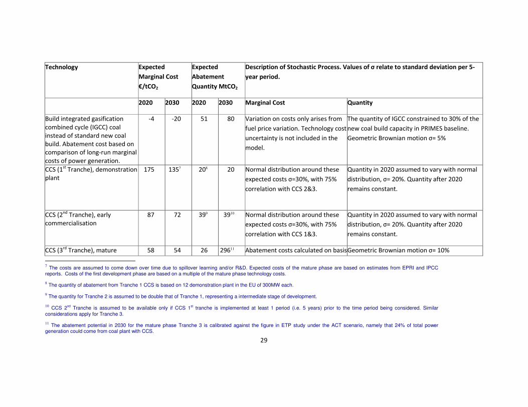
29

Technology Expected

Marginal Cost

€/tCO2

Expected

Abatement

Quantity MtCO2

Description of Stochastic Process. Values of σ relate to standard deviation per 5-

year period.

2020 2030 2020 2030 Marginal Cost Quantity

Build integrated gasification

combined cycle (IGCC) coal

instead of standard new coal

build. Abatement cost based on

comparison of long-run marginal

costs of power generation.

-4 -20 51 80 Variation on costs only arises from

fuel price variation. Technology cost

uncertainty is not included in the

model.

The quantity of IGCC constrained to 30% of the

new coal build capacity in PRIMES baseline.

Geometric Brownian motion σ= 5%

CCS (1st Tranche), demonstration

plant

175 1357 208 20 Normal distribution around these

expected costs σ=30%, with 75%

correlation with CCS 2&3.

Quantity in 2020 assumed to vary with normal

distribution, σ= 20%. Quantity after 2020

remains constant.

CCS (2nd

Tranche), early

commercialisation

87 72 399 3910 Normal distribution around these

expected costs σ=30%, with 75%

correlation with CCS 1&3.

Quantity in 2020 assumed to vary with normal

distribution, σ= 20%. Quantity after 2020

remains constant.

CCS (3rd

Tranche), mature 58 54 26 29611 Abatement costs calculated on basis Geometric Brownian motion σ= 10%

7 The costs are assumed to come down over time due to spillover learning and/or R&D. Expected costs of the mature phase are based on estimates from EPRI and IPCC

reports. Costs of the first development phase are based on a multiple of the mature phase technology costs.

8 The quantity of abatement from Tranche 1 CCS is based on 12 demonstration plant in the EU of 300MW each.

9 The quantity for Tranche 2 is assumed to be double that of Tranche 1, representing a intermediate stage of development.

10 CCS 2

nd Tranche is assumed to be available only if CCS 1

st tranche is implemented at least 1 period (i.e. 5 years) prior to the time period being considered. Similar

considerations apply for Tranche 3.

11 The abatement potential in 2030 for the mature phase Tranche 3 is calibrated against the figure in ETP study under the ACT scenario, namely that 24% of total power

generation could come from coal plant with CCS.

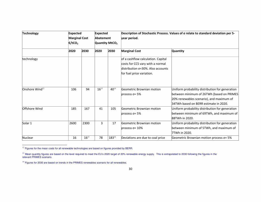
30

Technology Expected

Marginal Cost

€/tCO2

Expected

Abatement

Quantity MtCO2

Description of Stochastic Process. Values of σ relate to standard deviation per 5-

year period.

2020 2030 2020 2030 Marginal Cost Quantity

technology of a cashflow calculation. Capital

costs for CCS vary with a normal

distribution σ=30%. Also accounts

for fuel price variation.

Onshore Wind12 106 94 1613 4014 Geometric Brownian motion

process σ= 5%

Uniform probability distribution for generation

between minimum of 26TWh (based on PRIMES

20% renewables scenario), and maximum of

34TWh based on BERR estimate in 2020.

Offshore Wind 185 167 41 105 Geometric Brownian motion

process σ= 5%

Uniform probability distribution for generation

between minimum of 69TWh, and maximum of

88TWh in 2020.

Solar 1 2600 2300 3 17 Geometric Brownian motion

process σ= 10%

Uniform probability distribution for generation

between minimum of 5TWh, and maximum of

7TWh in 2020.

Nuclear 16 1615 78 18316 Deviations are due to coal price Geometric Brownian motion process σ= 5%

12

Figures for the mean costs for all renewable technologies are based on figures provided by BERR.

13 Mean quantity figures are based on the level required to meet the EU’s 2020 target of 20% renewable energy supply. This is extrapolated to 2030 following the figures in the

relevant PRIMES scenario.

14 Figures for 2030 are based on trends in the PRIMES renewables scenario for all renewables.

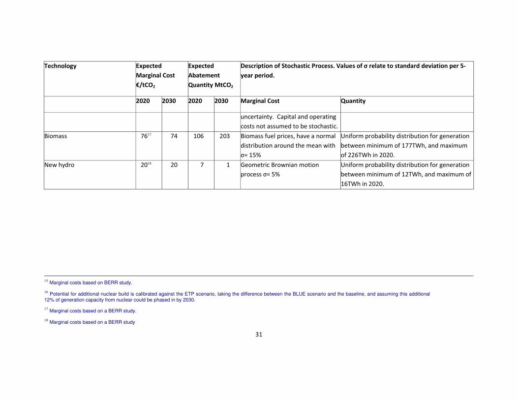
31

Technology Expected

Marginal Cost

€/tCO2

Expected

Abatement

Quantity MtCO2

Description of Stochastic Process. Values of σ relate to standard deviation per 5-

year period.

2020 2030 2020 2030 Marginal Cost Quantity

uncertainty. Capital and operating

costs not assumed to be stochastic.

Biomass 7617 74 106 203 Biomass fuel prices, have a normal

distribution around the mean with

σ= 15%

Uniform probability distribution for generation

between minimum of 177TWh, and maximum

of 226TWh in 2020.

New hydro 2018 20 7 1 Geometric Brownian motion

process σ= 5%

Uniform probability distribution for generation

between minimum of 12TWh, and maximum of

16TWh in 2020.

15

Marginal costs based on BERR study.

16 Potential for additional nuclear build is calibrated against the ETP scenario, taking the difference between the BLUE scenario and the baseline, and assuming this additional

12% of generation capacity from nuclear could be phased in by 2030.

17 Marginal costs based on a BERR study.

18 Marginal costs based on a BERR study

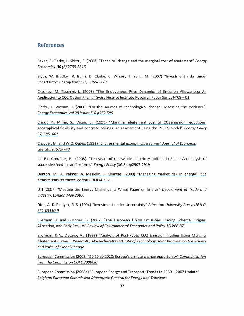
32

References

Baker, E. Clarke, L. Shittu, E. (2008) “Technical change and the marginal cost of abatement” Energy

Economics, 30 (6) 2799-2816

Blyth, W. Bradley, R. Bunn, D. Clarke, C. Wilson, T. Yang, M. (2007) “Investment risks under

uncertainty” Energy Policy 35, 5766-5773

Chesney, M. Taschini, L. (2008) “The Endogenous Price Dynamics of Emission Allowances: An

Application to CO2 Option Pricing” Swiss Finance Institute Research Paper Series N°08 – 02

Clarke, L. Weyant, J. (2006) “On the sources of technological change: Assessing the evidence”,

Energy Economics Vol 28 Issues 5-6 p579-595

Criqui, P., Mima, S., Viguir, L., (1999) “Marginal abatement cost of CO2emission reductions,

geographical flexibility and concrete ceilings: an assessment using the POLES model” Energy Policy

27, 585–601

Cropper, M. and W.O. Oates, (1992) “Environmental economics: a survey” Journal of Economic

Literature, 675-740

del Río González, P. (2008). “Ten years of renewable electricity policies in Spain: An analysis of

successive feed-in tariff reforms” Energy Policy (36:8) pp2907-2919

Denton, M., A. Palmer, A. Masiello, P. Skantze. (2003) “Managing market risk in energy” IEEE

Transactions on Power Systems 18 494-502.

DTI (2007) “Meeting the Energy Challenge; a White Paper on Energy” Department of Trade and

Industry, London May 2007.

Dixit, A. K. Pindyck, R. S. (1994) “Investment under Uncertainty” Princeton University Press, ISBN 0-

691-03410-9

Ellerman D. and Buchner, B. (2007) “The European Union Emissions Trading Scheme: Origins,

Allocation, and Early Results” Review of Environmental Economics and Policy 1(1):66-87

Ellerman, D.A., Decaux, A., (1998) “Analysis of Post-Kyoto CO2 Emission Trading Using Marginal

Abatement Curves” Report 40, Massachusetts Institute of Technology, Joint Program on the Science

and Policy of Global Change

European Commission (2008) “20 20 by 2020: Europe’s climate change opportunity” Communication

from the Commission COM(2008)30

European Commission (2008a) “European Energy and Transport; Trends to 2030 – 2007 Update”

Belgium: European Commission Directorate General for Energy and Transport

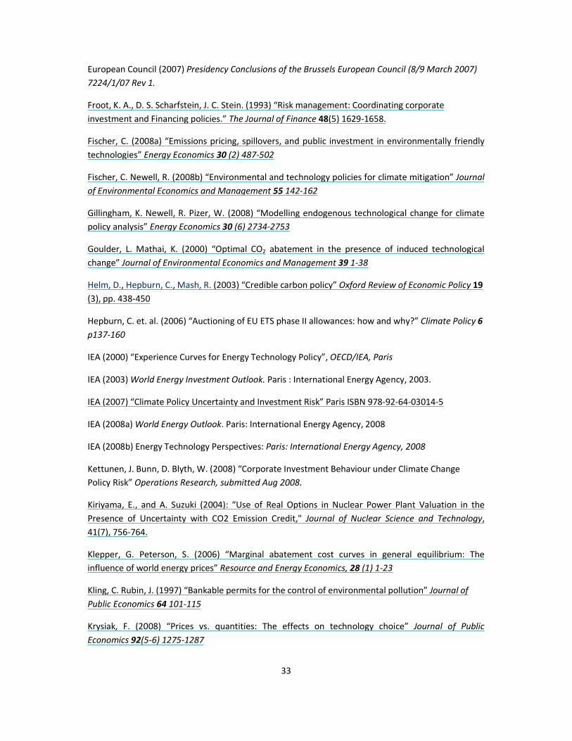
33

European Council (2007) Presidency Conclusions of the Brussels European Council (8/9 March 2007)

7224/1/07 Rev 1.

Froot, K. A., D. S. Scharfstein, J. C. Stein. (1993) “Risk management: Coordinating corporate

investment and Financing policies.” The Journal of Finance 48(5) 1629-1658.

Fischer, C. (2008a) “Emissions pricing, spillovers, and public investment in environmentally friendly

technologies” Energy Economics 30 (2) 487-502

Fischer, C. Newell, R. (2008b) “Environmental and technology policies for climate mitigation” Journal

of Environmental Economics and Management 55 142-162

Gillingham, K. Newell, R. Pizer, W. (2008) “Modelling endogenous technological change for climate

policy analysis” Energy Economics 30 (6) 2734-2753

Goulder, L. Mathai, K. (2000) “Optimal CO2 abatement in the presence of induced technological

change” Journal of Environmental Economics and Management 39 1-38

Helm, D., Hepburn, C., Mash, R. (2003) “Credible carbon policy” Oxford Review of Economic Policy 19

(3), pp. 438-450

Hepburn, C. et. al. (2006) “Auctioning of EU ETS phase II allowances: how and why?” Climate Policy 6

p137-160

IEA (2000) “Experience Curves for Energy Technology Policy”, OECD/IEA, Paris

IEA (2003) World Energy Investment Outlook. Paris : International Energy Agency, 2003.

IEA (2007) “Climate Policy Uncertainty and Investment Risk” Paris ISBN 978-92-64-03014-5

IEA (2008a) World Energy Outlook. Paris: International Energy Agency, 2008

IEA (2008b) Energy Technology Perspectives: Paris: International Energy Agency, 2008

Kettunen, J. Bunn, D. Blyth, W. (2008) “Corporate Investment Behaviour under Climate Change

Policy Risk” Operations Research, submitted Aug 2008.

Kiriyama, E., and A. Suzuki (2004): “Use of Real Options in Nuclear Power Plant Valuation in the

Presence of Uncertainty with CO2 Emission Credit," Journal of Nuclear Science and Technology,

41(7), 756-764.

Klepper, G. Peterson, S. (2006) “Marginal abatement cost curves in general equilibrium: The

influence of world energy prices” Resource and Energy Economics, 28 (1) 1-23

Kling, C. Rubin, J. (1997) “Bankable permits for the control of environmental pollution” Journal of

Public Economics 64 101-115

Krysiak, F. (2008) “Prices vs. quantities: The effects on technology choice” Journal of Public

Economics 92(5-6) 1275-1287

34

Lewis, M. (2008) “It Takes CO2 to Contango” Deutsche Bank Report

Mandell, S. (2008) “Optimal mix of emissions taxes and cap-and-trade” Journal of Environmental

Economics and Management 56 (2), pp. 131-140

Marklund, P. Samakovlis, E. (2007) “What is driving the EU burden-sharing agreement: Efficiency or

equity?” Journal of Environmental Management Volume 85, Issue 2, Pages 317-329

McKinsey & Company (2007) “Reducing U.S. Greenhouse Gas Emissions: How Much at What Cost?”

U.S. Greenhouse Gas Abatement Mapping Initiative, Executive Report December 2007.

Newell, R. Pizer, W. (2003) “Regulating stock externalities under uncertainty” Journal of

Environmental Economics and Management 45 (2 suppl) 416-432

Otto, V.M. Loschel, A. Reilly, J. (2008) “Directed technical change and differentiation of climate

policy” Energy Economics 30 (6) 2855-2878

Pindyck, R. (1999) “The long-run evolution of energy prices” The Energy Journal 20 (2)

Pizer, W. 2002 “Combining price and quantity controls to mitigate global climate change” Journal of

Public Economics 85, pp409-434.

Poyry (2008) “Compliance costs for meeting the 20% renewable energy target in 2020” Report to UK

Department of Business Enterprise and Regulatory Reform, March 2008

http://www.berr.gov.uk/files/file45238.pdf

Redpoint (2007) “Dynamics of GB Electricity Generation Investment” Report to DTI for Energy White

Paper http://www.berr.gov.uk/files/file38972.pdf

Reedman, L., P. Graham, P. Coombes. (2006) “Using a real-options approach to model technology

adoption under carbon price uncertainty: An application to the Australian electricity generation

sector” Economic Record 82 64-73

Richels, R. G. Blanford, G.J. (2008) “The value of technological advance in decarbonising the U.S.

economy” Energy Economics, 30 (6) 2930-2946

Roques, F.A., Nuttall, W.J., Newbery, D.M., de Neufville, R., Connors, S. (2006) “Nuclear power: A

hedge against uncertain gas and carbon prices?” Energy Journal 27 (4), pp. 1-23

Rosendahl, K. E. (2004) “Cost-effective environmental policy: implications of induced technological

change” Journal of Environmental Economics and Management 48 1099-1121

Rothwell, G. (2006) “A real options approach to evaluating new nuclear power plants” Energy

Journal, Vol. 27 No. 1 p37

Seifert, J. Uhrig-Homburg, M. Wagner, M.W. (2008) “Dynamic Behavior of CO2 Spot Prices” Journal

of Environmental Economics and Management, Vol. 56, No. 2, pp. 180-194

Sorrell, S., Sijm, J. (2003) “Carbon trading in the policy mix” Oxford Review of Economic Policy 19 (3),

pp. 420-437

35

Stankeviciute, L., Criqui, P. (2008) “Energy and climate policies to 2020: The impacts of the European

"20/20/20" approach” International Journal of Energy Sector Management 2 (2), pp. 252-273

Stern, N. 2007. The Economics of Climate Change: The Stern Review. Cambridge, UK: Cambridge

University Press

Weitzman, M.L. 1974 “Prices vs. Quantities” Review of Economic Studies 41 (4), 477-491

Yang, M., Blyth, W., Bradley, R., Bunn, D., Clarke, C., Wilson, T. (2008) “Evaluating the power

investment options with uncertainty in climate policy” Energy Economics 30 (4), pp. 1933-1950