Polarization Interactions and Boroxol Ring Formation in Boron Oxide: A Molecular Dynamics Study Janna K. Maranas * , Yingzi Chen Department of Chemical Engineering The Pennsylvania State University University Park, PA 16802 Dorothea K. Stillinger, Frank H. Stillinger Lucent Technologies 600 Mountain Avenue Murray Hill NJ 07974 We employ Molecular Dynamics simulations to study the structure of vitreous boron oxide. Although six- membered boroxol rings have been observed at fractions over 60% by various experimental techniques, simulation methods have not produced similar results.

Welcome message from author
This document is posted to help you gain knowledge. Please leave a comment to let me know what you think about it! Share it to your friends and learn new things together.
Transcript

Polarization Interactions and Boroxol Ring Formation in Boron Oxide:
A Molecular Dynamics Study
Janna K. Maranas*, Yingzi Chen
Department of Chemical Engineering
The Pennsylvania State University
University Park, PA 16802
Dorothea K. Stillinger, Frank H. Stillinger
Lucent Technologies
600 Mountain Avenue
Murray Hill NJ 07974
We employ Molecular Dynamics simulations to study the structure of vitreous
boron oxide. Although six-membered boroxol rings have been observed at
fractions over 60% by various experimental techniques, simulation methods have
not produced similar results. We adapt the polarization model, which includes
many body polarization effects thought to stablize such structures, for boron-
oxygen interactions. This model is then used in MD simulations of boron oxide
glass at various temperatures. We find a variation in the fraction of rings
depending on the temperature of the system during network formation. The
maximum ring fraction [>40%] occurs when the sample is prepared at low
temperatures. At these temperatures, the energy level of boron atoms in rings is

approximately 6% lower than the energies of boron atoms outside of rings. When
higher equlibration temperatures are used, the fraction drops to 11%. Thus, in
order to observe boroxol ring formation in simulations of boron oxide, a model
which incorporates polarization effects must be used and network formation
must occur at temperatures where ring formation is favored.
I. Introduction
Boron oxide [chemical formula B2O3] is a network glass-former. The short-range
structure of B2O3 is the planar BO3 triangle, where each boron atom is bonded to three
oxygen atoms with O-B-O angles of 120°. The intermediate-range structure, or the
arrangement of these triangles, has been established by various experimental techniques
as the planar boroxol ring, illustrated in Figure 1. Boroxol rings at fractions ranging from
f = 0.50 to f = 0.85 have been observed by inelastic neutron scattering (1,2), nuclear
magnetic resonance (3-6), nuclear quadrupole resonance (7-9), Raman scattering (10-20),
electron paramagnetic resonance (21,22) and diffraction techniques (23,24). Despite the
abundant experimental evidence for boroxol rings, the majority of molecular simulation
studies do not reveal such structures (25-33). A reverse Monte Carlo study (34) has shown
that a high percentage of boroxol rings cannot reproduce both structural data and density.
In one simulation study, a small percentage [approx. 12%] of boroxol rings were
observed (35) by including polarization of oxygen atoms. The other studies have
employed various two-body, three-body and in one case (Error: Reference source not
found) four-body potentials. In the four-body case, a ring fraction of 3% was observed.
One study using a three-body potential (36) cites a ring fraction of less than 20%.
No simulation study thus far has found a significant found fraction of boroxol
rings, and the reason for this is uncertain. One suggestion comes from the work of Teter
(Error: Reference source not found). This work used ab initio calculations to calibrate a
model for boron oxide. These calculations revealed that polarization of the oxygen atoms
is crucial in models of this type. Polarization is built into the Teter model by constructing
an oxygen ion as a central charge surrounded by four auxiliary charges in tetrahedral
symmetry. Within this simple representation of oxygen polarizability, the fraction of
boroxol rings increased from less than 1% to a final value of 12% as the magnitude of the
auxiliary charges was increased from zero. Thus for a simple ionic model, negligible ring
formation was observed, but as polarization effects are introduced, the ring concentration
rises.
One of us (37,38) has developed a more realistic model of polarizability. This
model incorporates a many body, non-additive interaction describing the dipole moments
induced by vibrational distortion. Polarization of oxygen ions thus arises from the other
ions present and is dependent upon their locations in the sample and thus its
configuration. Potentials for this model have been developed for Si4+, O2-, H+, and F- (39).
The MD program for this polarization model implements an alternative to periodic
boundary conditions that allows for simulation of chemical reactions. Conservative
external forces are used to provide what can be viewed as a “chemical reactor
containment vessel”. These forces act as semipermeable membranes the selectively pass
or block individual atomic species. This allows for a study of reactive processes with

automatic removal of reaction byproducts. The polarization model has been used to study
reactions and charge transfer processes in water (40-43) and recently has been applied to
silica glass (Error: Reference source not found). A description of the model is given in
Section II.
The current paper describes the application of the polarization model to the
simulation of vitreous boron oxide. We develop the necessary boron-oxygen and boron-
boron potentials by matching structural and energetic data of isolated boron-oxygen and
boron-oxygen-hydrogen molecules. This development is presented in Section III. We
describe in Section IV the application of this model to investigate the structure of boron
oxide. As with experimental preparation, we begin with an initial system of boric acid
[H3BO3] molecules, from which dehydration reactions occur, eventually ending with
boron oxide. The sample is then cooled, and a network structure develops. As expected,
the developing structure consists of BO3 triangles. Whether this network incorporates
boroxol rings is sensitive to the temperature at which the system is held during network
formation. In the temperature range where boroxol rings are energetically favored, we
find an experimentally relevant fraction of boroxol rings, f = 0.45.
II. Polarization Model Format
The task of the polarization model in the present context is to supply a chemically
flexible and realistic set of particle interactions to represent the formation and relaxation
behavior of boron oxide glasses. More generally, it is required to provide an
approximation to , the electronic ground-state potential energy surface for an arbitrary
configuration of N atomic particles that may include several elemental species. The
mathematical format chosen for the model permits full transferability, provided that the
particles remain essentially in the same oxidation (charge) state. In other words, the
model is constructed to allow the same set of basic particles to be assembled into a wide
variety of molecular or ionic species, and are capable of dynamic chemical interchange
between these combinations.
Several previous applications involving polarization model simulations have
appeared in print. These include several studies of water cluster structure and reactive
dynamics (Error: Reference source not found,Error: Reference source not found,Error:
Reference source not found,44), a similar study for hydrogen fluoride (45), and an
examination of phosphoric acid media (46). The present work involves an extension and
generalization of the previous polarization model version (Error: Reference source not
found, Error: Reference source not found), so for clarity and completeness we now
provide a detailed specification of the full mathematical format used for the boron oxide
glass application.
In the following will denote the positions of particles 1…N respectively,
Eq. 1
is the vector distance from to j, and
Eq. 2
is the corresponding scalar distance. Each particle i carries an electrostatic charge and
has a scalar polarizability ; these remain constant as the N-particle configuration of the

system changes. For some species (especially cations) it is expected on physical grounds
that the corresponding are negligibly small and can be set equal to zero, but for all
others it is positive. If particle possesses a nonvanishing polarizability, then generally
it will exhibit an induced dipole moment i that represents its response to the presence of
other particles and their moments, and that will vary as all particles execute their
dynamical motions.
The potential energy function comprises three types of contributions, each
dependent on the set of particle positions :
Eq. 3
The first two of these represent interparticle interactions; the third involves “wall forces”
that can selectively confine particles. Both and are chosen to vanish when all N
particles are far removed from one another.
Conventional applications of the molecular dynamics simulation technique, and of
the related Monte Carlo method (47), typically employ periodic boundary conditions to
eliminate the presence and influence of surfaces. However the simulation program
utilized here takes a different point of view, one in fact that parallels chemical and
chemical engineering practice. Conservative external forces are put in place to provide a
kind of “chemical reactor vessel”. The external forces can be manipulated so as to act as
semipermeable membranes that selectively pass or block individual atomic species. This
capacity permits the simulation of chemical reactions with automatic removal of reaction
byproducts; specific examples will appear below. Although it plays no role in the present

project, the capacity also exists to use appropriate conservative external forces to control
the shape of solid samples.
Central pair potentials compose the contribution :
Eq. 4
Although the subscripts and attached to the ’s nominally refer to specific
particles, it is only those particles’ species that matter in determining which pair function
to use; only three distinct species occur in the present application (boron, oxygen,
hydrogen). Furthermore, the ’s are invariant to subscript permutation:
Eq. 5
By themselves, the pair potentials in cannot realistically produce polyatomic
molecules such as H2O, B2O3, H3BO3, etc. with the correct bonding energies and
geometries. Inclusion of the many-body interaction rectifies the situation, however,
in particular allowing for the possibility of nonlinear and branched molecules (Error:
Reference source not found,Error: Reference source not found). The structure of
closely parallels that for the classical electrostatic interaction of charged, polarizable
point particles, but with short-range modifications that can account for the spatial

extension of electron clouds around the nuclei involved (Error: Reference source not
found,Error: Reference source not found). Specifically we have
.
Eq. 6
In the classical electrostatic precursor, all l’s are identically unity, so in the present
polarization model we therefore require
.
Eq. 7
Furthermore, general considerations require that the l’s should vanish as the cube of r at
the origin (Error: Reference source not found,Error: Reference source not found). Details
of chemical bonding behavior place constraints on the forms of these functions at
intermediate range (see the following Section III).
In contrast to the ’s, the short-range modification functions generally will not
possess subscript interchange symmetry, i.e. may not be the same as . As Eq.
6 above illustrates, we adhere to the convention that the first subscript ( ) refers to a

particle whose electrostatic charge is at issue, while the second subscript ( ) refers to a
particle whose induced moment ( ) is required.
Polarization model equations for determining the set of induced moments
similarly parallel the classical electrostatic formalism (Error: Reference source not
found,Error: Reference source not found). Once again short-range modification factors
(now denoted by ’s) are introduced to account for the spatial extent of electron clouds.
Consequently the induced dipole vectors have values determined by simultaneous linear
relations of the form:
Eq. 8
where
Eq. 9
Here is a dyadic tensor
Eq. 10
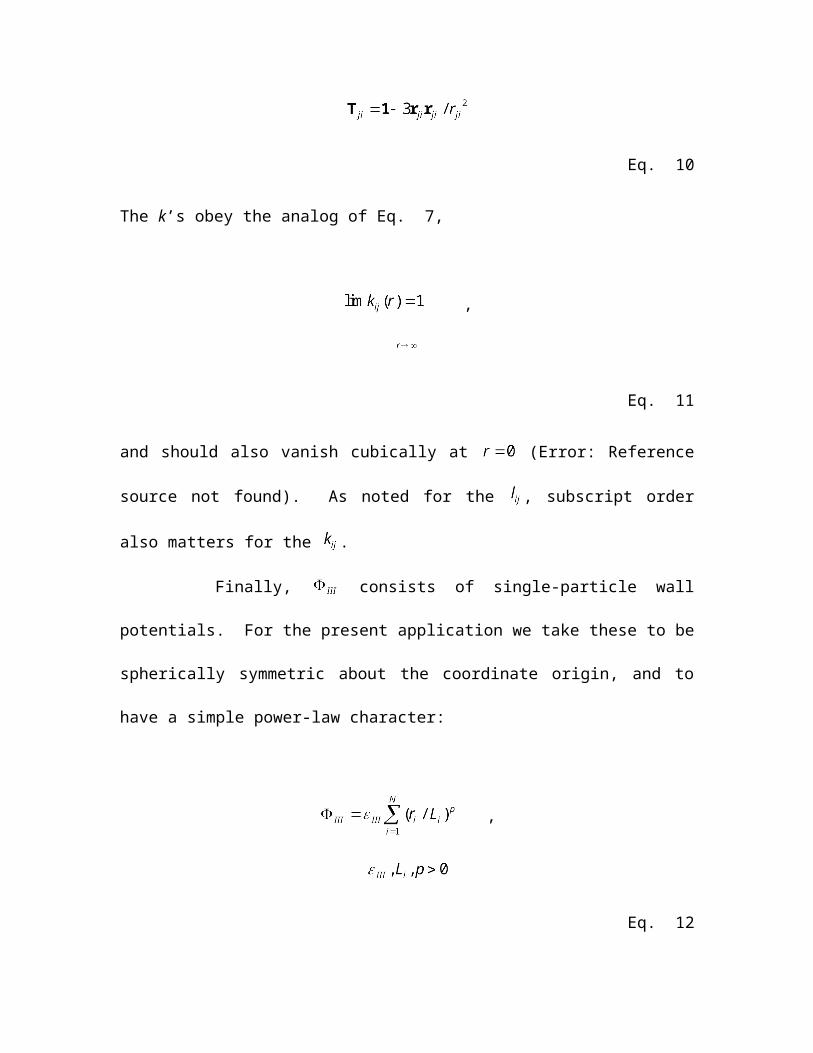
The k’s obey the analog of Eq. 7,

,
Eq. 11
and should also vanish cubically at (Error: Reference source not found). As noted
for the , subscript order also matters for the .
Finally, consists of single-particle wall potentials. For the present application we
take these to be spherically symmetric about the coordinate origin, and to have a simple
power-law character:
,
Eq. 12
The “semi-permeable membrane” feature introduced earlier involves assigning different
values to the for distinct particle species. Those with small remain confined to a
small neighborhood around the origin, while those with large are essentially free to
roam over a larger spherical neighborhood. The choice of positive exponent p determines
the wall steepness.
Classical molecular dynamics simulation follows the time evolution of an N-body
system, utilizing the Newtonian equations of motion,

Eq. 13
along with suitable initial conditions. Here is the mass of particle , and is the
total vector force exerted on particle . In the present context we have
Eq. 14
Because the forces are conservative, total energy remains constant in time, and the extent
to which a numerical integrator for Eq. 13 satisfies this property constitutes a measure of
its accuracy. Furthermore, the potential energy as specified above has full rotational
symmetry about the coordinate origin, so total angular momentum should also be
conserved. This latter attribute would disappear if a different, non-spherical, shape were
to be selected for the “walls”.
The partial forces and have relatively compact expressions when put into
explicit form. The former consists of central pair forces exerted on from all other
particles:
Eq. 15
The latter is directed radially inward toward the origin:

Eq. 16
Obtaining explicit expressions for the is less straightforward. One reason concerns
the fact that the induced moments all depend upon the positions of every particle . The
chain rule for differentiation would seem to imply that operating on with the gradient
requires finding the corresponding gradients of induced moment components.
However, a simple transformation eliminates this complication. The polarization
potential can formally be augmented by an arbitrary linear combination of the
vectors , Eq. 8, to yield the function
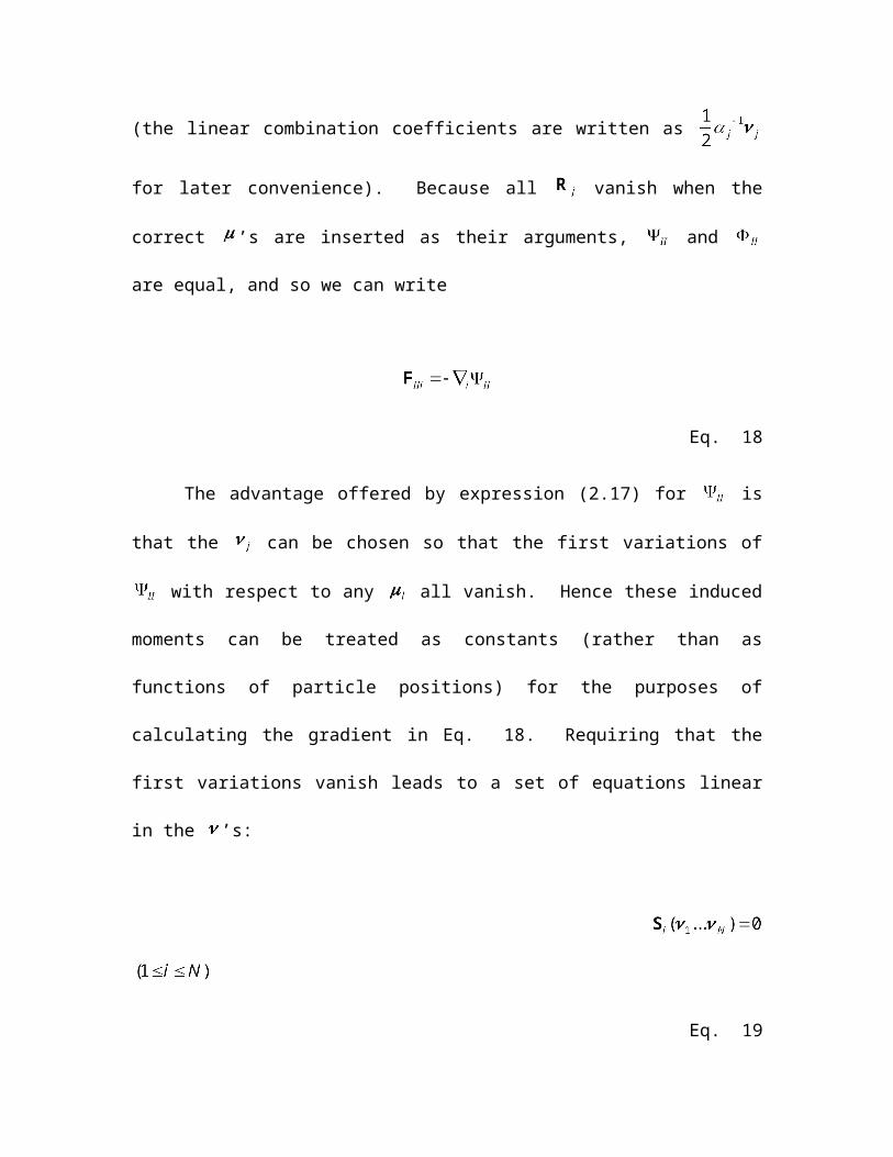
Eq. 17
(the linear combination coefficients are written as for later convenience).
Because all vanish when the correct ’s are inserted as their arguments, and
are equal, and so we can write
Eq. 18

The advantage offered by expression (2.17) for is that the can be chosen
so that the first variations of with respect to any all vanish. Hence these induced
moments can be treated as constants (rather than as functions of particle positions) for the
purposes of calculating the gradient in Eq. 18. Requiring that the first variations vanish
leads to a set of equations linear in the ’s:
Eq. 19
where
Eq. 20
The similarity between this set of equations for the and the prior set Eq. 8 - Eq.
9Eqs. (2.8)-(2.9) for the is inescapable, and invites naming these ’s “pseudo-
dipoles”. But notice that the differ from the by (a) replacement of by in the
sum over charges, and (b) subscript reordering (from to ) in the sum over (pseudo)
dipoles.
Evaluating the right member of Eq. 18 is straightforward but tedious. The resulting
terms can be collected in the following way:

Eq. 21
Notice that each of these contributions to the force on particle has formally been
identified with a specific other particle . Superscripts , , and for each
of these “pair” terms refer respectively to interactions between a charge and a dipole, a
charge and a pseudo-dipole, and a dipole and a pseudo-dipole. We find that the first of
these appears as follows:
Eq. 22
The second type has a similar form, except that ’s replace ’s, and ’s replace ’s:
Eq. 23
The third kind of pair contribution in Eq. 21 is the following:
Eq. 24
The last part of this expression has been displayed explicitly as separate Cartesian
components, with unit vectors along the x, y, and z directions denoted by , , and
respectively. The matrices have forms that appear in Appendix A. This
completes the specification of the forces needed to integrate the Newtonian equations of
motion.
In order to facilitate chemical interpretation of the N-particle configurations
encountered during the molecular dynamics simulations, it is useful to introduce a
geometric convention for the presence of chemical bonds in the system. The two types of
bonds expected in the present context are those involving a pair of particles bearing
opposite charges, namely OH, and OB. For the purposes of bond enumeration and of
graphical presentation we define a bond to exist if the corresponding pair distance is less
than 1.2 Å for OH, and less than 1.55 Å for OB. The reader should note that these cutoff
distances substantially exceed equilibrium bond lengths so as to count interactions that
may have temporarily experienced significant vibrational stretching.
In addition to bond enumeration, the system configurations generated by solving
the Newtonian dynamical equations lead to “inherent structures” (local minima) by
means of a steepest-descent mapping on the hypersurface (48,49). These inherent

structures are mechanically stable arrangements of the N particles in space, and by
construction are free from vibrational deformation. The force expressions presented in
this Section are required in order to carry out the mapping of dynamical configurations to
inherent structures. A significant advantage of the inherent structures over the dynamical
configurations that spawn them is their lesser sensitivity to the arbitrarily-chosen bond
cutoffs in bond enumeration (50).
II. Development of Input Functions for B3+
For the simulations presented here, we require potentials to describe all
interactions between H+, O2-, and B3+. Table 1 shows the charges, polarizabilities and
masses assigned to these species. The masses correspond to the most abundant naturally
occurring isotope. The hydrogen ion is a bare proton, and thus assigning it a vanishing
polarizability is natural. The boron cation carries two electrons, which are tightly bound.
Hence, we have also taken the polarizability of B3+ as zero.
The pairwise potentials, ij(r) are required for all pairs, and the short-range
modification functions kij(r) and lij(r) are required when j has a non-zero polarizability.
The following potential functions have been previously developed (Error: Reference
source not found) and are given in Appendix B: OO(r), HO(r), kOO(r), kHO(r), lOO(r), and
lHO(r). The units used there and in the results to follow are kcal/mol for energy and Å for
length. The fundamental proton charge is these units is e = [322.1669 Å kcal/mole]1/2.
This section describes the development and subsequent testing of the remaining input
functions: BB(r), BO(r), BH(r), kBO(r), and lBO(r). The strategy we employ for
assignment of the functions is to optimize the fitting of properties of isolated molecules.
We have used structural data [bond lengths, bond angles] for BO+ (51), HBO2 (52,53,54)

B2O3 (Error: Reference source not found,Error: Reference source not found,55,56) and
H3BO3 (57,58,59) and the dipole moment, dipole derivative and harmonic force constant for
BO+(Error: Reference source not found). The structures resulting from the model
potentials were assessed by use of the MINOP procedure to determine the minimum
energy structure.
37. F.H. Stillinger, C.W. David; J. Chem. Phys. 69, 1473 (1978).
38. F.H. Stillinger; J. Chem. Phys. 71, 1647 (1979).
39. F.H. Stillinger, D. Stillinger; private communication.
40. F.H. Stillinger, C.W. David; J. Chem. Phys. 73, 3384 (1980).
43. T.A. Weber, F.H. Stillinger; Phys. Rev. Lett. 89, 154 (1982).
47. Simulation of Liquids and Solids, edited by G. Ciccotti, D. Frenkel, and I.R. McDonald (North-Holland, New York, 1987).
48. F.H. Stillinger and T.A. Weber, Phys.Rev. A28, 2408 (1983).
49. F.H. Stillinger, Science 267, 1935 (1995).
50. F.H. Stillinger and T.A. Weber, J. Chem. Phys. 88, 7791 (1988).
1. A.C. Hannon, D.I. Grimley, R.A. Hulme, A.C. Wright, R.N. Sinclair; J. Non-Cryst. Solids 177, 299 (1994).
2. M. Massot, S. Souto, M. Balkanski; J. Non-Cryst. Solids 182, 49 (1995).
3. G.E. Jellison Jr., L.W. Panek, P.J. Bray, G.B. Rouse Jr.; J. Chem. Phys. 66, 802 (1977).
6. J. W. Zwanziger, U. Werner-Zwanzinger, C. Joo; Abstracts of Papers of the Amer. Chem. Soc., 218, 43-GEOC (1999).
7. S. J. Gravina, P.J. Bray, G.L. Petersen; J. Non-Cryst. Solids 132, 165 (1990).
9. P.J. Bray, J.F. Emerson, D. Lee, S.A. Feller, D.L. Bain, D.A. Feil; J. Non-Cryst. Solids 129, 240 (1991).
10. F. Galeener, G. Lucovsky, J.C. Mikkelsen, Jr.; Phys. Rev. B 22, 3983 (1980).

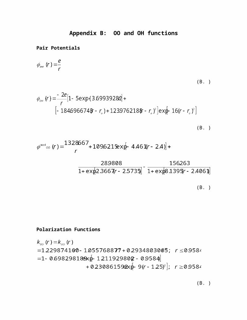
Pairwise Potentials
The pair interactions are dominated at large distances by the Coulomb interaction
between appropriate charges:
20. E.I. Kamitsos, M.A.Karakassides; Phys. Chem. Glasses 30, 19 (1989).
21. Y. Deligiannakis, L. Astrakas, G. Kordas; Phys. Rev. B, 58, 11420 (1998).
22. I.A. Shkrob, B.M. Tadjikov, S. D. Chemerisov, A.D. Trifunac; J. Chem. Phys. 111, 5124 (1999).
23. P.A.V. Johnson, A.C. Wright, R.N. Sinclair; J. Non-Cryst. Solids 50, 281 (1982).
24. R.L. Mozzi, B.E. Warren; J. Appl. Cryst. 3 251 (1970).
25. ?. W. Soppe, C. van der Marel, H.W. den Hartog; J. Non-Cryst. Solids 101, 101 (1988).
33. R. Fernández-Perea, F.J. Bermejo, M.L. Senet; Phys. Rev. B 54 6039 (1996).
34. J. Swenson, L. Börjesson; Phys. Rev. B 55, 11138 (1997).
35. M. Teter; Proc. Second Int. Conf. On Borates Glasses, Crystals and Melts, 407 (1996).
36. R.E. Youngman, J. Kieffer, J.D.Bass, L. Duffrène, Jour. Non.-Cryst. Solids, 222, 190 (1997).
44. T.A. Weber and F.H. Stillinger, J. Chem. Phys. 77, 4150-4155 (1982).
45. F.H. Stillinger, Int. J. Quantum Chem. 14, 649-657 (1978).
46. F.H. Stillinger, T.A. Weber, and C.W. David, J. Chem. Phys. 76, 3131 (1982).
51. K. A. Peterson, J. Chem. Phys. 102, 262 (1994).
52. M. J. S. Dewar, C. Jie and E.G. Zoebisch, Organometallics 7, 513 (1998).
53. M. J. S. Dewar and M.L. McKee, J. Am. Chem. Soc., 99, 5231 (1977).
At short separations, these functions diverge to infinity due to repulsion. For
pairs of species where chemical bond formation is possible, this function should have a
minimum at the equilibrium bond length. The starting point for assignment of pair
potential functions are these limiting features.
The boron-boron interaction is left as:
However, the boron-hydrogen interaction required modification to increase
repulsion at small distances. Without this modification the H-O-B angle in HBO2 was
much smaller than available experimental data suggests is appropriate (Error: Reference
source not found). The final form
represents a compromise between known H-O-B angles in HBO2 and H3BO3.
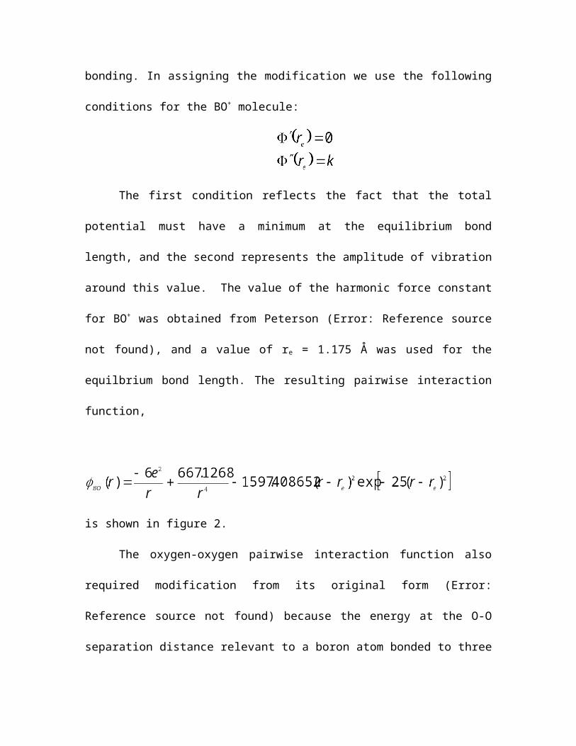
In the oxygen-boron interaction, there must be a modification that reflects the
potential for chemical bonding. In assigning the modification we use the following
conditions for the BO+ molecule:
54. F. Ramondo, L.Bencivenni and C. Sadun, Journal of Molecular Structure, 209, 101 (1990).55. M.T. Nguyen, P Ruelle and T.-K. Ha, Journal of Molecular Structure, 104, 353 (1983).
56. A.V. Nemukhin and F. Weinhold, J. Chem. Phys. 98, 1329 (1993).
57. W.H. Zachariasen, Acta Crystallogr. 16, 385 (1954).
58. T.T. Merzlyak, Journal of Molecular Structure, 344, 171 (1995).59. A.S. Zyubin and S.A. Dembovsky, Glass Physics and Chemistry, 21, 178 (1995).

The first condition reflects the fact that the total potential must have a minimum at
the equilibrium bond length, and the second represents the amplitude of vibration around
this value. The value of the harmonic force constant for BO+ was obtained from Peterson
(Error: Reference source not found), and a value of re = 1.175 Å was used for the
equilbrium bond length. The resulting pairwise interaction function,
is shown in figure 2.
The oxygen-oxygen pairwise interaction function also required modification from
its original form (Error: Reference source not found) because the energy at the O-O
separation distance relevant to a boron atom bonded to three oxygens was large enough to
prevent 3-fold coordinated boron atoms. The O-O repulsion was lessened by an amount
that results in a B-O bond distance in 3-fold coordinated molecules which is as close as
possible to known values (60) [approx. 1.37 Å]. We also required that the geometry of the
water dimer (which was used to make the initial assignment) was changed as little as
possible. This modified function is also given in Appendix B.
Polarization Functions
The polarization functions have been assigned with the limiting values in Section
II: namely that both lBO and kBO approach unity at large distances and vanish cubically at r
= 0. For kBO, we consider the dipole moment of BO+:

Numerical values for the dipole moment and dipole derivative (Error: Reference source
not found) were used to assign the function:
We choose lBO such that the total energy of the B2O3 molecule has a minimum at
the B-O-B angle for which there is the most evidence, = 137º (Error: Reference source
not found,Error: Reference source not found).
Both the k and l functions for BO interactions are plotted in Figure 3.
Verification of Function Choices
The function choices outlined above were confirmed by comparisons of model-
generated minimum energy structures with experimental and ab initio structures for B2O3,
HBO2, and H3BO3, as discussed above, and for H3B3O6 (Error: Reference source not
found,Error: Reference source not found) and H4B2O5 (Error: Reference source not
found). Results for B2O3, H3BO3 and HBO2 are shown in figure 4. In all cases, the
magnitudes of double and single B-O bonds are higher than comparable data suggests.
However, we have preserved the difference between the double and single bond lengths
of approximately 0.1 Å. The single B-O bond also increases in going from 2-fold to 3-
fold coordination, in agreement with available structural data. A comparison of relative
energy values between molecules is given in Table 2. This also indicates reasonable
agreement with available data.

Section IV: Application to Boron Oxide Structure
The polarization model with the function assignments described in Section III was
used to carry out Molecular Dynamics calculations as described in Section II. The initial
system consisted of 81 boric acid [H3BO3] molecules arranged in a regular array of
approximately 10 x 10 x 16 Å. The molecules are spaced by 5 Å along the two directions
paralell to the plane of the molecule and 2 Å perpendicular to this plane. This selection
of initial system allows us to closely follow the normal experimental preparation method
for boric acid glass, namely dehydration of boric acid. All particle velocities were
initially set to zero. In all simulations described here, a time step of 0.2 fs was used. The
wall parameters in III [Eq. 12] were chosen as
LO = LH = 40.0 Å
LB = 20.0 Å
These selctions were made so that as water molecules are formed via dehydration
reactions, they are free to leave the “reaction zone”, while species containing boron
remain. As the gear algorithm began to advance the system in time, the boric acid
molecules quickly decomposed, primarily through the following reactions:
H3BO3 H2O + HBO2 = -211.4
2 HBO2 B2O3 + H2O = -248.6
As these reactions are highly exothermic, the temperature of the system rose strongly and
velocity scaling between runs was used to keep the temperature in the neighborhood of
6000 K. As the simulation proceeded, water molecules accumulated outside of the
reaction zone. These molecules interact only weakly with the inner core, however their
presence places computational demands on the molecular dynamics simulation program.

For this reason, the simulation was periodically stopped for removal of these molecules
from the system. Other reactions occurred to a minor extent, resulting in the formation of
a few OH- groups. These were removed from the outer zone with the water molecules.
As the dehydration reactions proceeded, the L parameter for boron was decreased to
LB = 8Å
in stages.
After 64 ps at these conditions, no hydrogen remained in the system, which
consisted of the 81 boron atoms in the system initially, and 124 oxygen atoms; primarily
in the form of B2O3 molecules. A few linkages between molecules had formed and a few
BO3 triangles were present in the system. At this point, we began cooling the system from
the relatively high temperature [6000 K] used to facilitate dehydration. In this stage, the
L parameters were chosen so that the experimentally relevant density [1.84 g/cm3] was
maintained in the sample. This was chosen by determining the moment of intertia of the
sample and equating it to a hypothetical sphere of radius r and density 1.84 g/cm3. The
resulting radius was used to set the common L parameter for boron and oxygen. It was
then adjusted as necessary during the course of the remaining simulations to maintain the
proper density.
As the temperature was lowered in stages, the molecules began to arrange
themselves in a network formation comprised of BO3 triangles. Figure 5 illustrates the
extent of network formation at a temperature of 3500 K. Depicted in the upper snapshot
is the entire spherical simulation cell, while in the lower snapshot, portions of the cell are
separated to more easily view the forming network structure. As the temperature was
lowered further and network formation continued, two alternate procedures were used. In

procedure 1, the temperature was held at approximately 2000 K until most of the network
had formed[128 ps]. The temperature was then lowered again in stages, but at a much
lower cooling rate, to a final temperature of 1700 K. In this sample, one boroxol ring is
present in the final structure shown in Figure 6, although it did breakup and reform
during the course of the simulation. In procedure 2, the temperature was held at
approximately 1800 K while network formation was completed, and then cooled in stages
until 700 K. The final structure of this sample as illustrated in Figure 7 is markedly
different, with four boroxol rings and one 8-membered ring. Of the boron atoms in the
network structure with 3-fold coordination, this amounts to 44% in ring structures. This
value is consistent with experimental estimates of the fraction of boroxol rings
[approximately 40% at 800 K (Error: Reference source not found)].
To explain these observations, we have calcuated the energies of ring versus non-
ring 3-fold coordinated boron atoms at 2000 K and at 1700 K. These calculations are
summarized in Table 3. We use only 1 and II in determining these energies, as III
reflects the proximity of the structure in question to the hypothetical spherical container.
Since the ring structures are located primarily in the interior of the system, including the
wall energy would unfairly bias the results. These calculations show that ring structures
are energetically favored at 1700 K by about 6%, while at 2000 K, there is little
difference. This suggests that holding the system at high temperatures where ring
formation is not favored energetically as network formation occurs prevents the
formation of boroxol rings. Ring formation does not occur, even if the system is
subsequently cooled into the range where it is energetically favored, perhaps because of
an energy barrier or kinetic limitations for the transformation within the network. This
has obvious implications for simulation work, where high temperatures are often used for
equilibration. It should be noted that surface effects likely play a large role in our
simulations, as a network cluster as small as the one studied here must be dominated by
surface effects. Since the rings in our cluster are all located in the interior, it is likely that
a cluster absent of surface effects would have larger ring concentration.
The pair distribution functions for the high temperature [no rings] and low
temperature structures are compared in Figure 8. The O-O, O-B and B-B correlations are
shown. Differences resulting from the presence of rings are minor. Both the O-O and O-
B distributions have an additional small peak when rings are present. In the O-B
distribution, this peak appears at 2.8 Å, the position of the nearest O-B separation in a
ring [see Figure 1]. In the O-O distribution, this peak appears at 4.2 Å, the next nearest
O-O separation in a ring [see Figure 1].
Figure 9 shows the average energy obtained from the simulation runs as a
function of the average temperature. Also shown in the Figure are the energies of the
“inherent structures”, obtained by subjecting the final system configuration in each run to
the MINOP procedure. There are no obvious differences in the two configurations. At
high temperatures, the energies are relatively insensitive to temperature, but in the range
3000 K – 1500 K, the energies change more rapidly with temperature, eventually
reaching a low temperature plateau. It should be noted that the low temperature runs are
most likely not equilibrium structures due to time limitations of computer simulations.
This type of change in energy is indicative of glass formation, and the small changes
observed here are consistent with a strong glass former, as well as with a fast cooling
rate.

Section V: Discussion and Concluding Remarks
This study has applied the polarization model to investigate the intermediate-
range structure in boron oxide, a network glass-former regarded as strong in the
classification scheme of Angell. This model allows for polarization of oxygen atoms by
the surrounding boron atoms, and is thus inherently a many body potential. The selection
of input functions to the model was made on the basis of isolated molecules containing
boron, oxygen and hydrogen. With these selections, the polarization model predicts
structural properties [ie, bond lengths and angles] within 5% of their known values.
Perhaps more importantly than numerical agreement is the agreement of trends within
structural features; for example the difference in the B-O bond length between 2-fold and
3-fold coordinated boron atoms. One should not expect that any simulation model would
perfectly correlate numerical values of experimental observables, but an accurate
representation of trends among these observables is a good measure of model
performance.
Having set and tested the model input functions, we used the polarization model
to investigate the network structure in boron oxide glass. The formation of a trigonal
network in boron oxide as the temperature is lowered closely parallells experimental
observations of the glass transition. Based on a large number of experimental studies, this
network is thought to consist to a large extent of boroxol rings, with the concentration of
boron atoms in rings increasing through the transition region. However, the presence of
ring fractions in excess of the high temperature limit [approx 20%] has not been
confirmed with computer simulation where direct observation is possible. We prepared
vitreous nanobeads by dehydrating boric acid [a common experimental precursor] and
quenching into the region where significant motion is not observed over the time scale of
our simulations. The temperature range over which a transition to the vitreous state is
observed in these simulations, 1500 – 3000 K, is displaced significantly from the
corresponding range [500 – 1200 K] of experimental observations. This is expected in
light of the extremely short time scales observable via computer simulation [on the order
of nanoseconds] and the even shorter time scales accessible in the present simulations
[approx 0.3 ns total for the longer low T run]. It is likely that the energy drop off in
Figure 9 would continue, were additional computer time available for longer equilibration
at the lower temperatures. Simulations of this nature are currently underway. The onset of
network formation occurs around 3000 K, i.e. it coincides with the onset of the transition
region. As the energy drops through the transition range, network formation becomes
more complete. However, even at the lower end of this transition, the system is not fully
interconnected.
In these simulations, we observe that the creation of boroxol rings occurs at the
time of network formation. Boroxol rings form at temperatures less than about 2000 K,
about 1000 K lower than the onset of network formation. An energetic analysis shows
that ring structures are favored at temperatures lower than this cut-off. If the system is
held above 2000 K as network formation proceeds, ring structures are not incorporated in
the network structure. Subsequent cooling to temperatures where ring formation is
favored does not cause the network in place to rearrange itself into boroxol rings. In
contrast, if the system is held below 2000 K as the network structure forms, a significant
fraction of boroxol rings is incorporated. We find that the fraction of boron atoms in
rings is 44% for two average rates of cooling through the region 2500 – 1700 K. This

suggests that the fraction observed at 1700 K is not an artifact of a fast quench, although
the continuation of the faster cooling rate to lower temperatures likely arrests further ring
formation. The ring fraction of 44% corresponds to that observed experimentally at
approximately half of the temperature interval preceding the glass transition, i.e. at a
temperature around 800 K. We are currently continuing the simulations at lower
temperatures with longer equilibration times to test for additional ring formation.
We have calculated the pair distribution functions of the various types of atoms in
the simulation: O-O, B-B, and O-B, for the system with significant ring formation [44%
of boron atoms in rings], and no ring formation. The differences in the distributions are
minor, with small features appearing in the O-O and O-B distributions that correspond to
the cross-ring distances in boroxol rings. These minor differences may be difficult to
detect in x-ray diffraction measurements, where the O-O and O-B distributions are
smeared together. Evidently, the preferred separation distances in boron oxide networks
can be satisfied by both ring- and non-ring configurations.
We close with a comment on the cause of significant boroxol ring formation in
our simulations. We have employed a model that includes the effect of oxygen
polarization. It is tempting to attribute the observation of significant ring formation to the
level of realism in the model. However, ring formation is obviously sensitive to
temperature. Therefore, one cannot exclude the possibility that the temperature at which
network formation occurs is the primary contributor to ring formation. In other words, a
simulation done with a model that neglects polarization, yet carries out network
formation in the temperature range where ring structures are favored may result in
significant ring formation. This would seem to be the case in the simulations of

Youngman, et al (Error: Reference source not found). In addition, the fact that the major
stabilization in energy comes from the pairwise part of the potential [approx 90%], and
not the polarization part [about 10%], would seem to support this conclusion. However,
the polarization interactions may affect the location of atoms, and thus indirectly the pair
potentials. Further, the simulations of Teter (Error: Reference source not found) clearly
show that the fraction of boroxol rings is related to the extent of polarization of oxygen
atoms.
Appendix A
Equation (2.24) in the text above contains a set of matrices that have the
following explicit forms:
;
(A.1)
;
(A.2)
. (A.3)

Appendix B: OO and OH functions
Pair Potentials
(B. )
(B. )
(B. )
Polarization Functions
(B. )

Table 1: Fundamental properties of species. The polarizability for oxygen was obtained from reference Error: Reference source not found.
Species qi / e i (Å3) mi / mH
B +3 0.0000 11
O -2 1.444 16
H +1 0.0000 1

Table 2: Energies of molecules relative to H3BO3 from the polarization model and ab initio calculations.
Energy Polarization model Reference Reference
(H3B3O6) / (H3BO3) 2.19 2.12 2.027
(H4B2O5) / (H3BO3) 1.716 1.675 ----

Table 3: Energetics of boroxol ring formation. All energies are in kcal/mole.
Potential
T = 1925 K T = 1975 K
rings non-rings rings non-rings
I -1901.5 -1801.5 -1891.28 -1895.54
II -179.39 -157.02 -176.76 -157.09
I + II -2081.24 -1958.52 -2068.04 -2052.51

Figure 1: A schematic illustration of a boroxol ring

Figure 2: The boron-oxygen pair potential, BO(r).

Figure 3: Polarization funtions for boron-oxygen interactions. Solid symbols: lBO(r). Open symbols: kBO(r).

Figure : Structural properties of isolated molecules. a: HBO2, b: B2O3, c: H3BO3.
Figure 4 a: HBO2
Figure 4 b: B2O3
Figure 4 : Structural properties of isolated molecules. a: HBO2, b: B2O3, c: H3BO3.
Property Polarization Model Experiment
x(Å) 1.07 0.9611y(Å) 1.35 1.33z(Å) 1.27 1.22HOB(deg) 118.32 125.7
Figure 4a: HBO2.
Property Polarization Model Experiment
x(Å) 1.26 1.20y(Å) 1.36 1.33BOB (deg) 136 137
Figure 4b : B2O3.

Figure 4 c: H3BO3
Property Polarization Model Experiment
x(Å) 1.038 0.900y(Å) 1.416 1.362
Figure 4c: H3BO3.

Figure 5: The boron-oxygen system at 3440 K. The dark atoms are B3+ and the light are O2-. A boron-oxygen bond is drawn if the separation is less than 1.55 Å.

Figure 6a: The boron-oxygen system formed at high temperature. The dark atoms are B3+
and the light are O2-. A boron-oxygen bond is drawn if the separation is less than 1.55 Å.
Figure 6a: The boron-oxygen system formed at high temperature. The dark atoms are B3+
and the light are O2-. A boron-oxygen bond is drawn if the separation is less than 1.55 Å.

Figure 6 b: The same system as Figure 6a with the large sections pulled apart so their structure may be more easily seen.
Figure 7a: The system formed at low temperature. The dark atoms are B3+ and the light are O2-. A boron-oxygen bond is drawn if the separation is less than 1.55 Å.
Figure 7dummy label

Figure 7 b: The same as Figure 7a with large clusters pulled apart to more easily see their structure. Four boroxol rings and one 8-membered ring are present. This amounts to 44% of boron atoms in ring structures.

0
5
10
15
20
25
30
0 1 2 3 4 5 6 7
r (A)
g(r)
grOBgrOB
low T high T
0
0.5
1
1.5
2
2.5
3
2.5 3 3.5 4
r (A)
g(r)
grOBgrOB
low T high T
Figure 8 a: The boron-oxygen pair distribution function for low temperature (boroxol ring formation) and high temperature (no ring formation) preparations. The inset is a blowup of the region where small differences due to ring formation appear.

0
2
4
6
8
10
0 1 2 3 4 5 6 7r(A)
g(r)
grOOgrOO
high Tlow T
0
2
4
2.5 3 3.5 4 4.5 5
r(A)
g(r)
grOOgrOO
high Tlow T
Figure 8b: The oxygen-oxygen pair distribution function for low temperature (boroxol ring formation) and high temperature (no ring formation) preparations. The inset is a blowup of the region where small differences due to ring formation appear.

0
1
2
3
4
5
6
0 1 2 3 4 5 6 7
r(A)
g(r)
grBBgrBB
high Tlow T
Figure 8c: the boron-boron pair disturbution function for low temperature (boroxol ring formation) and high temperature (no ring formation) preparations.
60. L. Pauling, The Nature of the Chemical Bond, (Cornell University Press, Ithaca, 1960).
Figure 8: Potential energy as a function of temperature. Both the average energy from the simulation run, and the inherent structure energy found by minimizing the energy from the ending coordinates are shown.

Related Documents