POLAR SYMMETRIC FLOW OF A SVISCOUS COMPRESSIBLE … · x-622-74-124 preprint nasa ti xze 72 polar symmetric flow of a sviscous compressible atmosphere; an application to mars joseph

X-622-74-124PREPRINT

NASA TI XZE 72

POLAR SYMMETRIC FLOW OF ASVISCOUS COMPRESSIBLE ATMOSPHERE;

AN APPLICATION TO MARS

JOSEPH A. PIRRAdLIA -

074-26920

(WS-X-70672) ~POLAB SYM gME IC FLOW

OF A VISC3US COPESIBLE ATOSPEBE; nclasAPPLICAII O AiS (IASA) - P HC UnclaS$5I.25 y0 G3/1 3 42164

MAY 1974

GODDARD SPACE FLIGHT CENTERGREENBELT, MARYLAND

https://ntrs.nasa.gov/search.jsp?R=19740018807 2019-08-25T12:18:26+00:00Z

For information concerning availabilityof'this document contact:

Techliical Information Division, Code 250Goddard Space Flight CenterGreenbelt, Maryland 20771

(Telephone 301-982-4488)

POLAR SYMMETRIC FLOW OF A VISCOUS

COMPRESSIBLE ATMOSPHERE;

AN APPLICATION TO MARS

Joseph A. Pirraglia

May 1974

The Laboratory for Planetary Atmospheres

Goddard Space Flight Center

Greenbelt, Maryland

i

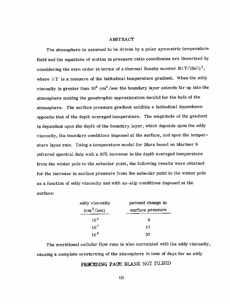
ABSTRACT

The atmosphere is assumed to be driven by a polar symmetric temperature

field and the equations of motion in pressure ratio coordinates are linearized by

considering the zero order in terms of a thermal Rossby number RAT/(2al) 2,

where A T is a measure of the latitudinal temperature gradient. When the eddy

viscosity is greater than 106 cm 2 /sec the boundary layer extends far up into the

atmosphere making the geostrophic approximation invalid for the bulk of the

atmosphere. The surface pressure gradient exhibits a latitudinal dependence

opposite that of the depth averaged temperature. The magnitude of the gradient

is dependent upon the depth of the boundary layer, which depends upon the eddy

viscosity, the boundary conditions imposed at the surface, and upon the temper-

ature lapse rate. Using a temperature model for Mars based on Mariner 9

infrared spectral data with a 30% increase in the depth averaged temperature

from the winter pole to the subsolar point, the following results were obtained

for the increase in surface pressure from the subsolar point to the winter pole

as a function of eddy viscosity and with no-slip conditions imposed at the

surface:

eddy viscosity percent change in

(cm 2/sec) surface pressure

106 9

10 7 17

108 37

The meridional cellular flow rate is also correlated with the eddy viscosity,

causing a complete overturning of the atmosphere in tens of days for an eddy

PRECEDING PAGE BLANK NOT FILMED

iii

viscosity of 10 8cm2 /sec and in hundreds of days for 106 cm 2 /sec. The implica-

tion of this overturning in the dust storm observed during the early part of the

Mariner 9 mission is discussed briefly.

iv

CONTENTS

Page

1. INTRODUCTION .................................... 1

2. DYNAMIC EQUATIONS ............................... 3

3. METHOD OF SOLUTION .............................. 9

4. TEMPERATURE FIELD AND BOUNDARY CONDITIONS ......... 11

5. NUMERICAL RESULTS ............................... 14

6. DISCUSSION OF RESULTS ............................. 20

ACKNOWLEDGMENTS ........ ......................... 23

APPENDIX I ......................................... 24

APPENDIX II ........................................ 26

REFERENCES ......... .............................. 27

V

1. Introduction

Zonal geostrophic motion of the atmosphere is often used as the basic flow

upon which more complex flow regimes are constructed. Its simplicity and, in

many cases, apparent approximation of observational data makes it an attractive

assumption. However, as a basic state a more adequate description may some-

times be desirable. As will be shown, if the atmosphere is vertically unstable

such that a large eddy viscosity is probable, the layer within which the geo-

strophic approximation is valid is confined to the upper regions of the atmos-

phere thereby eliding a large mass of the atmosphere from the assumed basic

state. Differential heating in the latitudinal direction of a rotating inviscid

planetary atmosphere causes zonal geostrophic motion with the result that there

is no latitudinal redistribution of mass. However, when viscosity or damping

are introduced geostrophy is disrupted and there is a resultant meridional flow

with a latitudinal pressure gradient that is no longer arbitrary as in geostrophic

flow which adjusts itself to any imposed pressure field. The linearized dynamic

equations with the viscous terms retained predict Hadley cell circulation in

addition to the zonal motion, the geometry and flow associated with the cells

being dependent upon the temperature gradient and the magnitude of the viscous

terms.

Polar symmetric flow as a limiting case of tidal theory with damping was

considered for Mars by Pirraglia and Conrath (1974). Linear damping propor-

tional to the velocity was assumed and the shearing stress terms were ignored

which precluded the possibility of satisfying the horizontal velocity boundary

conditions at the surface. The latitudinal surface pressure gradient turns out to

be independent of the magnitude of the damping coefficient and dependent upon

1

only the gradient of the vertically mass averaged temperature. On the other hand,

the wind field, in particular the meridional component, is strongly dependent upon

the damping coefficient. The use of a linear damping term gives a poor descrip-

tion of the upper atmosphere where it does not predict predominantly geostrophic

flow.

Differentially heated fluids in rotating annuli have been treated by Robinson

(1959) and Barcilon and Pedlosky (1967a, 1967b) among others. In these papers

the Boussinesq approximation is made and while Robinson discusses a homo-

geneous fluid, Barcilon and Pedlosky discuss a stratified fluid. Robinson ex-

pands the equations in terms of a thermal Rossby number and uses boundary

layer analysis where the Ekman number is the small parameter. Barcilon and

Pedlosky assume that the Rossby number is less than the Ekman number and

expand in 1/2 powers of the Ekman number with the dynamic variables being

sums of interior fields and boundary-layer corrections, which is equivalent to

the boundary-layer analysis. These latter papers indicate the striking effect of

stratification on rotating fluid flow as compared to the homogeneous case. (The

book by Greenspan (1968) gives a fairly extensive treatment of rotating fluids.)

In this paper we shall consider a formal solution to the Navier-Stokes

equations, with eddy viscosity in place of molecular viscosity, for polar sym-

metric flow in which the density is determined from the perfect gas law and the

atmosphere is in approximate hydrostatic equilibrium with vertical velocities

due to horizontal divergence. The problem is not approached as a boundary

layer problem since a substantial part of the total mass of the atmosphere

could be strongly influenced by the boundary conditions if the viscosity is large.

Spiegel and Veronis (1959) point out that a basic assumption of the Boussinesq

2

approximation is that the density variation through the depth of the atmosphere

is small compared to the average density. Since this is not true for the full depth

of the atmosphere, in addition to the fact that to the zero order we will consider

an essentially homogeneous condition, the Boussinesq approximation is not used.

The linearized zero order solution is the first iteration of a set of nonlinear

integrodifferential equations whose resultant flow is a combination of Hadley

cell circulation, an Ekman-like velocity profile and approximate geostrophic

flow at high altitudes.

Specific results are presented in which the temperature field is based upon

temperature data obtained by the infrared spectroscopy experiment on Mariner 9

and the eddy viscosity is assumed to be constant with altitude. The results of this

application show the dependence of latitudinal pressure gradient upon the tem-

perature field, the magnitude of the eddy viscosity and the boundary conditions.

Also shown is the correlation of the thickness of the boundary layer with the

eddy viscosity, independent of the boundary conditions, and the meridional flow

rates associated with the eddy viscosity and boundary conditions. From the re-

sults one can determine the validity of the geostrophic approximation under

differing conditions and the difficulty due to boundary condition uncertainties,

in predicting the flow within the outer boundary layer in even a relatively simple

model. The meridional flow rates lead to speculations concerning the dust storm

observed during the early part of the Mariner 9 mission.

2. Dynamic Equations

The problem to be considered is the time invariant symmetric state of a

rotating shallow viscous atmosphere with an imposed polar symmetric tempera-

ture field. Effects of curvature are neglected and the atmosphere is assumed

3

to be very close to being in vertical hydrostatic equilibrium and to obey the

perfect gas law. To simplify the analysis the equations will be expressed in

o -coordinates (Phillips, 1957) where the vertical coordinate a is the ratio of

the atmospheric pressure at altitudes within a column to the pressure at the

base of the column.

The following symbols are defined:

v horizontal velocity vector on a constant a-plane,

a vertical velocity,

-u surface pressure,

T temperature,

o geopotential,

Te radiative equilibrium temperature,

7 radiative relaxation time,

R gas constant for atmosphere,

c, specific heat of atmosphere at constant pressure,

K R/cp

6 colatitude,

¢ longitude,

a vertical coordinate,

H mean pressure scale height,

KM momentum eddy diffusivity,

KH heat eddy diffusivity,

k unit vertical vector,

L rotational speed of planet,

a radius of planet,

4

6 cosine of the colatitude,

V horizontal gradient operator.

The symbols v, 5 , T, 7, D and V with asterisks are dimensioned variables

and without asterisks are dimensionless variables.

If the eddy diffusivity terms are of the form

1 av*pKm (1)p -z z

1 - P T * (2)p z 3zp

then using the mean pressure scale height H in place of an altitude dependent

scale height (1) and (2) can be written in c -coordinates as

a 2 T* T

L2 * (4)O-H2

If H were the true scale height the expressions (3) and (4) would be exactly

equivalent to (1) and (2) but are reasonable approximations if the mean scale

height is used.

Using (3) and (4), the time invariant equations describing the flow are

2 KV v * * RT* , __ 2 v* (

2 × + x v* + v* v + + V(* + i V * 7T * _ - 2 K m (5)70 -au H 2 0_

- KMV*2 V* = 0

5

* =-R Tds + (D (6)S

= _ * (7*7v*) ds (7)

Q c + T* RT* .*'a [ -2 - (a T* T (8)p- P * PP 0 \ - -I0 (-)

T* - T*- C pV* 2T* +C e

T

where in (6) and (7) s is an integration variable. The vertical velocity 5* is

equal to zero at the planet's surface o- = 1 and at the top of the atmosphere

a = 0 . The boundary conditions on the horizontal velocity will be expressed

as a linear combination of the velocity and its vertical shear equal to v* at-a

a = co and v * at cr = 1. The energy equation (8) is assumed to be radiatively0 -b

damped as expressed in the last term on the right hand side with the radiative

equilibrium temperature specified everywhere and the dynamically induced

temperature specified on the boundaries.

Using the average surface pressure 70 to define the dimensionless pressure

7r = 7T */o, and using the maximum latitudinal temperature difference AT to

define the speed U = RAT/(2aQ), the dimensionless variables v = v*/U, 5 = & *

(a/U) and T = T*/AT are defined. The dimensionless gradient operator is

defined by V = aV *. Using the dimensionless quantities in equations (5) through

(8) and defining a thermal Rossby number P = RAT/(2a f )2 and an Ekman

number E = KM /(2 H 2 ), the dimensionless dynamic equations are

6

6kx v +/3( Vv + o. + V+TV in- e - eV2v= 0 (9)

=-1 V" (7v) ds (10)

D= - Tds. (11)1

With the Prandtl number P = KM /KH and the dimensionless radiative damping

time constant T = 2 f2 7* the dimensionless heat equation is

P =,8P VT 24K T-TP Q=lP~ 'VT+r-K a+ +-- -K t0- Tp-. (12)20c AT a i] "2 7

The temperature field is assumed to be the sum of an imposed temperature

field To = Te independent of the large scale dynamics and the temperature 8 T8

which is due to the dynamics. Then with T = To + 8 T8 (12) can be expressed as

e- -K + 6-- 2 T - - T+CT---KT + v' InP .C a a 2 T T )]13)

The square of the ratio of the scale height to the planet radius being a very

small number, the horizontal diffusion terms in (9) and (13) can be neglected.

With this approximation and using a Green's function involving integration in c-

only, the set of equations (9), (10), (11) and (13) can be expressed as a set of

7

integrodifferential equations which can be solved iteratively. Here we shall be

concerned with the velocity only to the zero order in / and with the temperature

field to the first order. In the zero order approximation To is the temperature

field driving the system and the dynamically induced temperature T is obtained

from (13) using the zero order terms in the right hand side of the equation.

With T = To and using the perfect gas law, equations (10), (11) and the zero

order momentum equation,

k xv - E - 0- + V(+ TV ln T= 0, (14)

form a complete set, sufficient to solve for the horizontal and vertical velocities

and the surface pressure. Equation (14) represents the balance between the

pressure, coriolis force and viscous effects. In regions in which 6 or E are

large compared to P the nonlinear terms of (9) can be neglected. Such regions

would be those sufficiently far from the equator or in the boundary layer where

there is appreciable wind shear. When E is of the order of unity1 equation (14)

is a good approximation over all regions except at very high altitudes in the

equatorial plane. For smaller values of e the linearized equations are a good

approximation in all regions except practically the full depth of the equatorial

zone.

Although the fluid is compressible, the zero order flow is essentially the

same as homogeneous flow since a moving parcel of fluid assumes the ambient

1For example if Mars with a 10 km scale height had an eddy diffusivity of 108 cm2 /sec E wouldbe of the order of .5 and /3approximately .05.

8

temperature imposed by the zero order temperature field. The motion would

be nonisentropic if it were assumed that heat is supplied or extracted so as to

maintain the zero order temperature. However, if it is assumed that the only

heating is that necessary to maintain the zero order temperature without the

flow, as stated above, and if the dynamic contribution Tp is small the flow is

still essentially homogeneous but adiabatic. When Tp is appreciable compared

to T o its effect on the flow must be considered and the phenomena associated

with stratification will become apparent. In our formulation such effects would

be determined iteratively.

3. Method of Solution

Expressing the velocity v in complex form v = v¢ + ive , where v8 is the

meridional velocity and v € is the zonal velocity, and using the symmetry of the

applied temperature field, equation (14) in complex form is

-iL(2 Y) + v : + T In 7T F (15)

The boundary conditions on v(cx) are

(a) v(cr0 ) cos aa + v'(cr0 ) sin aa = v a

(16)

(b) v(1) cos a b + v' (1) sin a b = Vb

where the prime indicates the derivitive with respect to or. The choice of

a a , ab , v and vb allows the boundary conditions to be specified in terms of

the velocity, the velocity shear or a linear combination of the velocity and

shear. The Green's function solution of (15) is discussed in Appendix I.

9

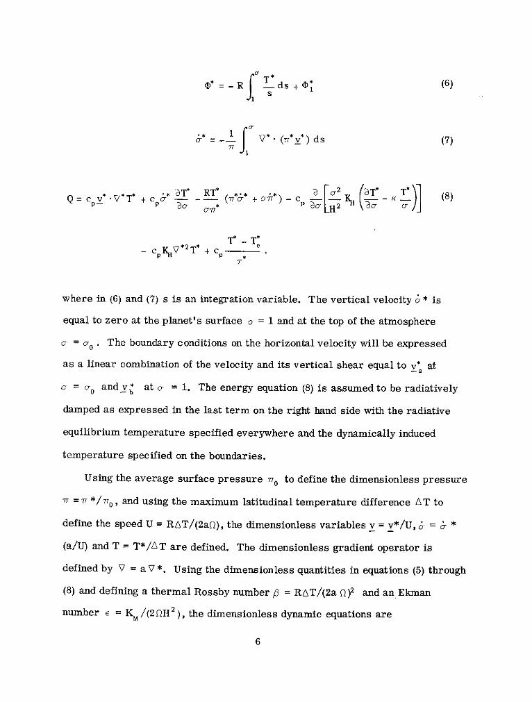
Letting G represent integration over the homogeneous Green's function

and Ga and Gb the boundary contributions, the solution to (15) is

v = G(F) + GbVb + GaV a . (17)

Assuming that any surface velocity will be proportional to the surface pressure

gradient we can write vb = Sb - / e In 7T. Similarly, assuming that conditions

at the top of the atmosphere will be dependent upon the surface pressure and the

geopotential we define va = S a/0 Inn + vaO. The terms Sa, Sb and vao will

be defined below. From the definition of F in (15) and the preceeding discussion,

v = G + TI n 7 T) + GSb n+ a Inn + Vao (18)

The continuity equation (10) for steady symmetric flow is

( v ds = 0 (19)

and implies

S o Vgds = constant, (20)

but since the mass flux across a meridional circle must be zero and ir 7 0

Svds = Im f vds Av = 0 (21)

where A represents taking the imaginary part of the integration over c.

10

Now using (18) in (21) the solution for the gradient of the surface pressure

is obtained;

AG (-30) + AGaV 03 ln a soo(22)

- In 7T = -_ (22)3 AG(T) + AGbSb + AG.S.

Then substituting (22) into (18) the velocity is solved for in terms of the applied

temperature field. Thus, equations (18) and (22) represent the solution to the

zero order dynamic problem once the polar symmetric temperature field and

the boundary conditions have been defined.

4. Temperature field and Boundary Conditions

The dimensionless temperature field is assumed to be of the form

To = Ts + (Tt + T1P1 (O) + T2 P2 (O)) cY (23)

where P1 and P2 are first and second degree Legendre polynominals of the

first kind. T, represents the stratospheric temperature, T t is the globally

averaged temperature at the surface and T P1 and T2 P2 are the equatorially

symmetric and asymmetric parts respectively.

From equations (11) and (23) and with a prime on the Legendre function

indicating differentiation with respect to 0 the colatitudinal derivative of the

geopotential function is

- (T1P, + T2 P2 ) - + . (24)

11

We shall assume that cr = 1 is a constant geopotential surface and define

g1 = 0. Obviously, polar symmetric topology for which all the assumptions

made are still valid can easily be treated, but topology will be considered in a

subsequent paper.

Equation (24) gives the temperature and surface geopotential contributions

to (18) and (22) and all that is required to complete the solution is the velocity

boundary conditions.

At the surface the boundary condition will be imposed on the velocity alone

by taking sin ab = 0 and v(1) = vb in (16b). The surface velocity vb is assumed

to obey the equation

fk x b + TbV in 77 + 8vb = 0. (25)

where Tb is obtained from (23) with c = 1 and 8 is a damping coefficient.'

Defining the complex velocity vb = Vb¢ + ivbe the solution to (25) is

Vb =T i in 7 (26)62 +82 TB

and from the relationship between vb and Sb given preceeding (18)

Sb = Tb (27)62 + 82

ilf we assume the eddy viscosity in a shallow boundry layer of depth zb is equal to k U. Z, wherek is von Karman's constant, U. the friction velocity and z the altitude (Monin and Yaglom, 1971),then by dimensional argument / 2 z (kU.z v */-z),, kU*/zb vbU and 8 =kU./2R zb.

12

At the top of the atmosphere the two most reasonable choices of boundary

conditions are to make the velocity geostrophic or impose a condition of zero

shear. As ob - 0 the two are equivalent. Therefore (16a) with va = 0 and

cos a = 0 will satisfy the shear condition exactly and the geostrophic condition

very closely when a0 is very small. We can in fact take the top off the atmos-

phere and let oo = 0 and both conditions will be satisfied. The geostrophic

condition leads to the existance of a singularity in the velocity at 0 = 0 in the

equatorial plane, but the behavior in regions away from the singularity is not

grossly affected and the pathological behavior at high altitudes in the equatorial

plane will be tolerated. With va equal to zero, both va and Sa appearing in

(18) and (22) are identically zero.

Having defined the temperature field and the boundary conditions the surface

pressure and wind fields can be calculated.- Substituting (23) and (24) into (22)

and (18) we get

- 1 (T 1 P' + 2P2) [AG(1)- AG(or)] (28)

,BI -y TsAG(1) + (Tt + T1 P, + T2P2 ) AG(c&) + AGbSb

and

v = (TP' + T2P 2 G (1) - -G(_) + [TG(1 ) + (T t + T P +T2P2) G(c) + Gb Sb] n . (29)

Using the definition of the operators G and A and the function Gb all the terms

of (28) and (29) are easily calculated and the horizontal velocity and the surface

pressure are expressed in terms of the Ekman number, the parameters of the

13

temperature field and the damping coefficient. The vertical velocity is calculated

from (10) using the results obtained in (28) and (29).

The first order temperature field can be calculated from equation (13) after

the zero order velocities have been determined. Designating the terms in the

brackets on the right hand side of the equation by QD and neglecting the hori-

zontal diffusion term, the first order equation is

a2T aT2 T+ (2 - K) - - (K + (30)aa2 aa- T)T E QD

where

P(T -E)

Assuming Tp is zero at o- = c-0 and - = 1, (30) is solved in a manner similar

to (15). The details are given in Appendix II.

5. Numerical Results

In applying the analysis of the preceeding sections three values of eddy

viscosity KM = 10 6 , 10 and 10 cm2 /sec (E = .006, .06 and .6) are used to

represent what might be from slightly to extremely unstable conditions in the

atmosphere. With each value of eddy viscosity two surface boundary conditions

are considered, the conditions being no-slip (vb = 0) or the surface velocity

controlled by a linear damping term as indicated in (29). The latitudinal

behavior of the surface pressure is calculated under the six combinations of

viscosity and boundary conditions for a model of a temperature field based on

the Mariner 9 infrared spectrometer data (Hanel, et al, 1972).

14

The vertically averaged temperature is shown in the top part of Figure 1. In

accordance with (23) the temperature field is T = 150 + (395/6-45/2P, -85/3 P2 ) o. 4

The parameters chosen give temperatures of 1500, 1650, 2300 and 2100 Kelvin

in the stratosphere and at the base of the atmosphere at the north pole, equator

and south pole respectively. This roughly approximates the diurnally averaged

Martian atmospheric temperatures during the dissipation of the dust storm

(Hanel, et al, 1972). The two lower parts of Figure 1 show the ratios of surface

pressure to globally averaged surface pressure associated with the three values

of eddy viscosity for both boundary conditions. From each section of the figure

the dependence of the pressure on viscosity is apparent while in all cases its

latitudinal behavior is opposite that of the vertically averaged temperature.

The reason for the increase in the pressure gradient resulting from an

increase in eddy viscosity can be seen from a simplification of (28). Assuming

that the vertical and horizontal temperature variations are small compared to T,

and neglecting the boundary term since it is not essential to the argument, (28)

can be expressed as

Im S-1/ 2 (1-x) 1 - S d s

T 1 P1 + T2P 2- n 77 - (31)

STs

IM f S-1/2 (l-x) ds

where Im S - 1/2 (l-x) can be viewed as weighting function. The vertical behavior

of the geopotential function (1 - S )/Y and the weighting function at 450 latitude

for KM = 106, 107 and 108 cm 2 /sec are shown in Figure 2. With the integral in

the denominator acting as a normalizing factor and the numerator being the

integrated product of the weighting and geopotential functions, the more overlap

15

between the two functions the larger the quotient of the two integrals will be.

Thus it is apparent from Figure 2 that larger pressure gradients are associated

with larger viscosities. The weighting function is a measure of the thickness

of the viscous dominated boundary layer. If e << 4 6 the weighting function is of

the form e (2 ') s i n ( 1/( 2 E) In cr) and has a negative one-half power Ekman

number behavior. Larger eddy viscosities cause thicker boundary layers in

which an increase mass of the atmosphere is freed from geostrophic flow and

has a meridional component. The increased shear resistance due to the larger

viscosity coupled with the greater mass in nongeostrophic flow results in an

increased pressure gradient.

Note also that the parameter y in the geopotential function has an effect

on the pressure gradient. Large values of y yield small pressure gradients

through the decrease of the effective depth of the atmosphere in which a hori-

zontal temperature gradient drives the circulation. To the zero order the effect

on surface pressure is not due to a change in the stratification and it is a different

effect than that discussed in Barcilon and Pedlosky (1967a, b). We have implicitly

assumed that eddy diffusion overwhelms convection and the flow is essentially

that of a homogeneous fluid as opposed to stratified flow (Greenspan, 1968,

124-132) as pointed out above. However, if the vertical temperature gradient is

sufficiently large, the higher order terms must be considered as was also

pointed out above.

Comparing the no-slip cases to the cases in which a surface velocity is

permitted indicates that the type of boundary condition also has an appreciable

effect on the surface pressure. The essentially smaller flow resistance in the

cases with non-zero surface velocity allows more mass flow near the surface

resulting in less piling up of the atmosphere at the poles and, consequently, a

smaller surface pressure gradient. The upper atmosphere tends to flow towards

the poles due to the downward slope of the constant pressure surfaces towards

the colder parts of the atmosphere while the surface pressure gradient causes

a return flow from the poles to the subsolar region.

Figure 3 indicates the rate at which the cellular flow turns over the atmos-

phere in the no-slip and finite surface velocity cases. Plotted for three values

of eddy viscosity is the percentage of the atmosphere that is exchanged across

a latitudinal circle normalized to the circumference of the latitudinal circle.

The large flow rates in the equatorial region for K equal to 10 6 and 107 are

not correct since for these cases both E and 6 are small and the non-linear 8

order terms should be included since all the velocity terms of (9) may be of the

same magnitude. Outside of the equatorial region where the coriolis term is of

appreciable magnitude, the results are a good approximation for all the values

of eddy viscosity.

In regions away from the equator there is approximately a tenfold increase

in the flow in going from KM = 106 to KM = 108 cm 2/sec. The implications of this

increase and the flow rates will be addressed later.

The cellular flows associated with the different values of eddy viscosity are

shown in Figures 4, 5, and 6. The atmosphere rises in the latitudinal band of

maximum temperature and descends at the poles, while associated with this

motion is a zonal flow generally geostrophic at high altitudes and oppositly

directed in the boundary layer which causes an atmospheric parcel to spiral

towards and away from the poles, the exact nature depending upon the viscosity

17

and the boundary conditions. As stated previously, the results in the equatorial

region are a poor approximation for K M = 106 and 107 cm 2/sec. The increased

meridional flow associated with a finite surface velocity is apparent when com-

parison is made between the no-slip and finite surface velocity conditions indi-

cated in Figure 3.

A comparison between Figures 4, 5 and 6 indicates the effect of the viscosity

and consequently the boundary layer thickness upon the cellular flow. The pole

to subsolar latitude flow takes place in the boundary layer while the subsolar

latitude to pole flow is in a region of approximate geostrophic flow as seen from

Figure 7. A change in viscosity changes both the altitude at which the north-

south flow changes direction and the latitude at which the ascending-descending

flow changes direction.

Figures 7 and 8 show some representative wind profiles. Figure 7 illustrates

the magnitude and direction of the horizontal flow at 400 north and south for three

values of eddy viscosity and zero-slip boundary conditions. Figure 8 illustrates

the analogous information for the boundary condition which allows a finite surface

velocity based on one day damping, 5 = .5/0. Figures 4 through 6 indicate that

there is always a small meridional flow except at a = 0 where the flow is geo-

strophic, while from Figures 7 and 8 the layers through which geostrophic flow

is dominant are clearly shown from the plots of the directions. Geostrophic flow

is indicated by the east direction and in Figures 7 and 8 it is seen to dominate

the upper 4/5 of the atmosphere when K M = 10 cm 2 /sec and the upper 1/2 and

1/10 when KM = 10 7 and 10s cm 2 /sec respectively. The thickness of the outer

boundary layer depends upon the Ekman number and is independent of the inner

boundary condition as is evident from the comparison of Figures 7 and 8. It

18

should be pointed out that the thickness also depends upon the latitude because

in the Green's function, which determines the influence of adjacent layers upon

one another, there appears exponents of a containing the term /E. Decreasing

the distance from the equator (decreasing 5) is equivalent to increasing the eddy

viscosity (increasing e) and subsequently increasing the boundary layer thickness.

While the thickness of the boundary layer is unaffected by the boundary

condition, the behavior within the layer is changed markedly with a change in

boundary conditions. For example, when KM = 107cm 2 /sec and a zero-slip

boundary condition is imposed, the wind vector rotates counter-clockwise through

approximately 900 with increasing altitude, as seen in Figure 7. When a surface

velocity is permitted, as in Figure 8, the wind vector rotates clockwise through

approximately 1200. In addition, when a surface velocity is permitted, in going

from KM = 106 to KM = 10 7 cm 2 /sec the wind vector rotates in opposite

directions.

Outside the boundary layer the wind profiles for each value of eddy viscosity

are all similar and are dependent upon the temperature field and only weakly

dependent on the boundary conditions through the differences in surface pressures.

Assuming a Prandtl number equal to unity the first order temperature field

was calculated for a variety of conditions. A sketch of the general form of the

isotherms representative of all the cases is shown in Figure 9. Figures 10 and

11 show temperature profiles at ±400 latitude for the three values of eddy vis-

cosity used previously and with radiative damping times of one and ten days.

The results shown are for a no-slip surface boundary condition. Having chosen

a Prandtl number equal to unity, KH = KM and E = K, /(2 Q H 2) = KH/(2 Q H2).

19

The parameter e appears explicitly as a coefficient in the equation for the first

order temperature in Appendix II and implicitly through hl, h 2 , J and the heating

term QD. Thus, as is apparent from Figures 10 and 11, the dependency of the

temperature on the eddy viscosities is not simple. In the regions poleward of

300 the effect of the smaller vertical velocity in decreasing the temperature is

partially offset by a decrease in heat diffusion, both being the result of smaller

eddy diffusion terms.

Comparison of Figures 10 and 11 indicate the larger first order temperature

associated with a decrease in the radiative damping.

When the eddy viscosity is 106 or 107 cm 2/sec the maximum and minimum

temperatures are of the order of tens of degrees and occur at high altitudes in

regions of large vertical velocities seen in Figures 5 and 6. For reasons stated

earlier these results are unrealistic since the nonlinear terms should be con-

sidered and the large gradients would have a significant effect on the dynamics,

but only within a limited region. With an eddy viscosity of 108 cm 2 /sec, the

minimum and maximum temperatures are -8 to +4 K for 7* = 1 and -10 to

+5 K for 7* = 10 and the gradients associated with these temperatures would not

have a significant effect on the dynamics. The main aspects of the flow would

remain unchanged.

6. Discussion of Results

Evidently a better description of the behavior of eddy viscosity with altitude

and an improved simulation of boundary conditions are needed in order to give

a better description of the wind profile, especially in the boundary layer, and

without a more definitive description of the radiative effects, it is difficult to

20

predict the temperature field in anything more than a qualitative manner. More

sophisticated models could have been used in the analysis but would have unduly

complicated the calculations at this stage of its development. In spite of the

simple treatment of the eddy viscosity and the boundary conditions, the latitudinal

pressure gradient and meridional flow rate are obviously correlated with the

boundary condition imposed at the surface and the vertical stability of the atmos-

phere as manifested in the eddy viscosity. In addition, the mechanism for a

polar temperature inversion is present.

For large values of eddy viscosity, the geostrophic approximation is a poor

one for the bulk of the atmosphere, but when the eddy viscosity is of the order

of 106 cm 2/sec or less the geostrophic approximation should be adequate if one

is concerned with the bulk of the atmosphere and not with the boundary layer.

As the equator is approached the approximation becomes poorer because the

boundary layer increases in thickness as pointed out above.

The dependence of the rate of overturning of the atmosphere on the eddy

viscosity has implications in the evolution of the great dust storm observed by

the Mariner 9 experiments at the time of the spacecraft's arrival at Mars in

November of 1971. (See the October 1972 issue of Icarus which is devoted

primarily to results obtained from Mariner 9 and Mars 2 and 3.) The dust storm

appears to have started about the time of maximum solar insolation which,

assuming that at that time the atmosphere was relative clear of dust, was on

the average a time of strong convective instability. Although the temperature

model used is supposedly representative of conditions during the dissipation of

the dust storm it may well represent the temperature structure during the

growth of the storm. In any event it will suffice for our argument since the

21

flow rates would not suffer an order of magnitude change with any reasonable

alteration of the temperature field. If the average eddy viscosity were as large

as 108 cm 2 /sec our model predicts a complete overturning of the atmosphere

on the order of tens of days. This is consistent with the ground based observa-

tions indicating a global spreading of the storm in approximately 15 days. When

dust becomes entrained in the atmosphere, the direct solar heating increases

(Gierasch and Goody, 1972) and the convective instability decreases. There is

evidence of this behavior indicated by the increasing lapse rate as the atmosphere

was clearing as observed by the infrared interferometer on Mariner 9 (Hanel,

et al, 1972). Conrath (1974) shows that an eddy viscosity of 10 7 cm 2 /sec is

consistent with the settling rate of the dust inferred by the secular variation of

the temperature. If the eddy viscosity decreases to 106 cm 2 /se e or less, the

time of overturning increases to hundreds of days. Thus, the most elementary

mode of the global dynamics appears to augment the processes that cause the

sudden growth and slow decay of the dust storm.

If the boundary conditions allow a velocity, as indicated in (32), the surface

winds directions are similar to the diurnal average of the near surface winds

shown in Pirraglia and Conrath (1974), which isn't surprising since both are

calculated in the same way. When the boundary layer is simulated by a thin

layer in which the viscosity is less than the viscosity of the upper layer, the

same type of wind pattern as mentioned above is obtained at the interface. In

the equatorial region this agrees rather well with the wind blown streaks seen

in the Mariner 9 television pictures (Sagan, et al, 1973). When a zero shear

boundary condition is used at the surface of the planet the surface pressure,

while still having the same qualitative behavior as before, then has a magnitude

22

independent of the eddy viscosity. The pressure is in fact identical to that found

using linear damping. The surface wind magnitude and direction are viscosity

dependent but nevertheless always lie in the quadrant giving general agreement

with the Mariner 9 television pictures.

We have compared our results with the numerical study of Leovy and Mintz

(1969) and there is a qualitative agreement of surface pressures in the ±35 O

latitude zone. The disagreement is at the poles, due to their including condensa-

tion and sublimitation of the atmosphere, which could be incorporated into our

model, and in the regions of baroclinic instability, which requires an extension

of our analysis to somehow parameterize the effect.

The approach presented did not consider the nonlinear terms or the possi-

bility of instabilities. In the limit of a very small Rossby number the results

should be a good approximation to the symmetric flow. Nevertheless, at this

time we do not know whether or not our model falls in the region of Rossby-

Ekman number parameter space where instabilities occur, assuming similarities

between a rotating sphere and the "qualitatively inferred" experimental results

shown in Robinson (1959) which indicate symmetrical stable, wave and eddy

regimes.

ACKNOWLEDGEMENTS

The author is grateful to Dr. B. J. Conrath for the many helpful discussions,

to Dr. R. A. Hanel for the suggestions concerning both the subject of this paper

and related areas, and to Prof. P. J. Gierasch for his comments. Part of the

work presented was performed during the author's tenure as a National Academy

of Sciences Resident Research Associate at NASA's Goddard Space Flight Center.

23

APPENDIX I

The solutions to the homogeneous form of (15) designated by w1 and w2 , w,

satisfying the homogeneous boundary condition at a = -o and w satisfying the

condition at - = 1, are

W1 =-1/2 (1- X) + C a-1/2 (I+X)

where

(1 - X) o01 sin aa - 2 cos aa

2 cos as - (1 + X) o 1 sin a

(1 - X) sin a b - 2 cos a bb 2 cos - (1 + X) sin ab

and X = /1 - 4 i/e .E The conjunct of w, and w is defined by

J =- iEo2 (wW 1 - Ww2) = iE(C b - Ca)

where the prime indicates differentiation with respect to -. If the solutions

w1 and w2 are linearly independent then the conjunct J is independent of a0. In

terms of the homogeneous solutions the solution to the inhomogeneous equation

(15) is

24

v -w2 ' y) - w1f I ' wl(°' ) f 1

v(r, ) = w(s, 0) F(s, 6) ds + J(0) w 2 (s, 0) F(s, 0) dsJ(0) J( )

0

w2 (1) sin % - w(1) cos ab+ iE v w, 8)(0-, )

w2 (J 0 ) sin as - wl(r 0 ) cos a.- i~ a 2 9)

where the integrals represent the Green's function solution for homogeneous

boundary conditions and the third and fourth terms are the contributions of the

inhomogeneous boundary condition (see Friedman, 1965).

The solution is dependent upon the choice of the eddy viscosity term (1) and

the particular choice leads to a relatively simple solution but, in fact, the eddy

viscosity terms can be more general and lead to more complicated solutions

than used here.

25

APPENDIX II

The homogeneous solutions to (30) are

h = /-D- (+K)+4 8T -D+

h2 = C-D- _- -D+

where

D+ = 1 [1-K + V(1 + K)2 + 4]

1D = [1 - K - V(1 + K)2 +48].

At both a = 1 and c = o hi and h2 are equal to zero. The conjunct of h1 and

h 2 is

JT = - / (1 + K) 2 + 48T (1 - o /(1 + K) 2 + 48T).

Using the homogeneous solutions to construct a Green's function, the solution

to (30) is

PT(, 2 () h (s) s-KQD(s , ) ds + h ( J ) h (S) S-KQ(S, ) ds0

26

REFERENCES

Barcilon, V., and J. Pedlosky, 1967a; Linear theory of rotating stratified fluid

motions. J. Fluid Mech., 29, 1-16.

Barcilon, V., and J. Pedlosky, 1967b; A unified linear theory of homogeneous

and stratified rotating fluids. J. Fluid Mech., 29, 609-621.

Conrath, B. J., 1974; to be published.

Friedman, B., 1965; Principles and Techniques of Applied Mathematics,

John Wiley & Sons, Inc., New York, 315 pp.

Gierasch, P. J. and R. M. Goody, 1972; The effect of dust on the temperature

of the Martian atmosphere. J. Atmos. Sci., 29, 400-402.

Greenspan, H. P., 1968; The Theory of Rotating Fluids, Cambridge Univ. Press,

London, 325 pp.

Hanel, R., et al., 1972; Investigation of the Martian environment by infrared

spectroscopy on Mariner 9. Icarus, 17, 423-442.

Leovy, C. and Mintz, Y., 1969; Numerical simulation of the atmospheric

circulation and climate of Mars. J. Atmos. Sci., 26, 1167-1190.

Monin, A. S. and A. M. Yaglom, 1971; Statistical Fluid Mechanics, MIT Press,

Cambridge, 769 pp.

Phillips, N. A., 1957; A coordinate system having some special advantages for

numerical forecasting. J. Meteor., 14, 184-185.

Pirraglia, J. A. and B. J. Conrath, 1973; Martian tidal pressure and wind fields

obtained from the Mariner 9 infrared spectroscopy experiment. J. Atmos.

Sci., 31, 318-329.

Robinson, A. R., 1959; The symmetric state of a rotating fluid differentially

heated in the horizontal. J. Fluid Mech., 6, 599-620.

27

Sagan, C., et al., 1973; Variable features on Mars 2, global results. J. Geophys.

Res.,. 78, 4163-4196.

Spiegel, E. A. and G. Veronis, 1960; On the Boussinesq approximation for a

compressible fluid. Astrophys. J., 131, 442-447.

28

225

00

u 175

0KM = 108 cm/se c ZERO SLIP

( 1.25 - BOUNDARY%, -'"... *:: CONDITION

r1.0-0Km = 10'

S .75 _Km = 106"

SI I I I.75 - KM = 1

90 60 30 0 -30 -60 -90

LATITUDE

Figure 1. Depth averaged temperature and surface pressures vs

latitude. Six conditions of eddy viscosity and surface boundaryconditions are represented in the two lower sections of the figure.

29

)Km =10

.2- K -

.4 0 1 2 3 5 .5 1

VALUE OF WEIGHTING FUNCTION 1--/

0- .1 .2 .3 A .5 0 .5 1

VALUE OF WEIGHTING FUNCTION 1 -b y

Figure 2. The influence of the boundary layer and the geopotential function vs altitude at 45'latitude. The surface pressure gradient is proportional to the quotient of the 0 -integratedproduct of the geopotential and weighting functions, and the o-integrated weighting function.

10.0,- ZERO SLIP BOUNDARY

8 \ CONDITION10 /

1.0 -0

1 1 00

.01

I I I I I

FINITE SURFACE10.0 10* VELOCITY

o 1.0

_ 10

.01

90 60 30 0 -30 -60 -90

LATITUDEFigure 3. Meridional cell flow rates as a function of latitude forthree values of eddy viscosity and two different boundary conditions.The flow rates represent the percentage of the total mass of the at-mosphere that is exchanged across a latitudinal circle in one daynormalized to the cosine of the latitude. In all cases, to the Northof -200 the flow at the surface is to the South and South of -200 theflow is to the North.

31

.24w T g ' F' g ~ \a ~ f

1.0 4 O *I 0" - - - 4 -40 -4. _4 D

90 60 30 0 -30 -60 -90

LATITUDE

Figure 4. Cellular flow pattern with no-slip boundary conditions and 10scm 2/sec eddy viscosity.An arrow length equal to the distance between arrow heads represents a velocity of 6.25m/secin the horizontal direction and a velocity of .2/cr cm/sec in the vertical direction.

1.0 * -1 i | 4 1I"'* 4 '" I4 4" " I

90 60 30 0 -30 -60 -90

LATITUDE

Figure 5. Cellular flow pattern with no-slip boundary conditions and 10 7cm 2/sec eddy viscosity.An arrow length equal to the distance between arrow heads represents a velocity of 6.25m/secin the horizontal direction and a velocity of .2/ cm/sec in the vertical direction.in the horizontal direction and a velocity of .2/a cm/sec in the vertical direction.

.2 r r4. 4 O r W 4

-,. 4'

u s p 4 . 4 . N u A' a g I- -- 44 4

4 ! - 4- I B I \ - - i I

1.0 -e. * i *l90 60 30 0 -30 -60 -90

LATITUDE

Figure 6. Cellular flow pattern with no-slip boundary conditions and 10 6 cm 2 /sec eddy viscosity.An arrow length equal to the distance between arrow heads represents a velocity of 6.25m/secin the horizontal direction and a velocity of .2/cr cm/sec in the vertical direction.

PROFILES AT 400 NORTH PROFILES AT 400SOUTH0 i i0 TF " 11 1 0 1 1 1 12 15.05 .2 16.74 .

E .4 -8.81 .4 9.92 w

.6 5.00 .6 5.68

S.8 2.22 .8 - 2.53 -

S10 LL 0 1.0 1 1 1 1 1 I 0

081 0 1 0 W 9"9 %

.2 15.05 .2- 16.74

E .4 8.81 .4 9.92 w.6 5.00 .6 5.68

.8 2.22 .8- 2.53

1.0 1/' 0 1.0 0

0 0 1 11

.2 15.05 .2 16.74

E .4 8.81 .4 9.92 w

S .6 5.00 .6 5.68

.8 2.22 .8 -2.53S 1.0 0 1.0 1 0111

0 20 40 60 80 WS E NW 0 20 40 6080 WS E NW

SPEED (m/sec) DIRECTION SPEED (m/sec) DIRECTION

Figure 7. Wind profiles vs altitude at 400 North and South latitudes with eddy viscositiesof 10 6, 10 7, and 10 cm2/sec and no-slip boundary conditions imposed at the surface.

PROFILES AT 4P NORTH PROFILES AT 40 0SOUTH

0 1 rrrr 0 TYTT i

2 -15.05 .2 -6.74 .

S.4 8.81 .4 - 9.92 w

.6 5.00 .6 5.68

1 222 .8 - n 2.53

01 0 rr r r2 15.05 2 16.74

E A 8.81 A 9.92 w

o .6 5.00 .6 -5.68.8- 2.22 .8- 2.53

1.0 )- l II , 0 1.0 10 1 1 1 I 1 0

0 02 15.05 .2 16.74

E 4 8.81 .4 9.92 w

.6 5.00 .6 5.682 - 22 .8- 2.53

S1.01 0 1.0 R 00 20 40 60 8W S E N W 0 20 40 60 80W S E NW "

SPEED (m/sec) DIRECTION SPEED (m/se) IWRECTON

Figure 8. Same as Figure 7 but with a finite surface velocity as described in the text.

1.0 .

.8 -

.6 -

.4.

90 60 30 0 -30 -60 -90LATITUDE

Figure 9. Isotherms of the first order temperature field. The shaded area is cooled,the rest is heated. The light lines represent .25K intervals the heavy lines 1.0Kintervals. The figure is a sketch of the case with KM = KH = 10 8 cm 2/sec. For smallervalues of eddy viscosities the form remains essentially the same while the magnitudeschange.

' ' ' ~~ '.............'

' ' ' ' ' ' ' ' ' '. ............'' '''............

valuesof ed y visc sitie the frm re ain.............................g itude.... ............

400 NORTH 4W SOUTH

.2-

/

.6

.8

1.0 1 I I

-1 0 1 2 3 4 5 6 7 8 -1 0 1 2

Tp(K) Tp(K)

Figure 10. First order temperatures with a one day radiative damping time constant

at 400 latitudes. The solid lines are for KM = 10 8 cm2 /sec, the dot-dashed for 10 7 and

the dashed for 106.

40 NORTH 400 SOUTH

.4- z

.6

.8 /

1.0 I I I0 1 2 3 4 5 6 7 8 -1 0 1 2

Tp(K) Tp(K)

Figure 11. First order temperatures with a ten day radiative damping time constantat ±40o latitudes. The solid lines are for KM = 10 8cm 2 /sec, the dot-dashed for 107

and the dashed for 106.