Poisson Parameters of Antimicrobial Activity: A Quantitative Structure-Activity Approach

Int. J. Mol. Sci. 2012, 13, 5207-5229; doi:10.3390/ijms13045207

International Journal of

Molecular Sciences ISSN 1422-0067

www.mdpi.com/journal/ijms

Article

Poisson Parameters of Antimicrobial Activity: A Quantitative

Structure-Activity Approach

Radu E. Sestraş 1, Lorentz Jäntschi

1,2,* and Sorana D. Bolboacă

3

1 University of Agricultural Science and Veterinary Medicine Cluj-Napoca, 3-5 Mănăştur,

Cluj-Napoca 400372, Romania; E-Mail: [email protected] 2 Technical University of Cluj-Napoca, 28 Memorandumului, Cluj-Napoca 400114, Romania

3 Department of Medical Informatics and Biostatistics, ―Iuliu Haţieganu‖ University of Medicine and

Pharmacy Cluj-Napoca, 6 Louis Pasteur, Cluj-Napoca 400349, Cluj, Romania;

E-Mail: [email protected]

* Author to whom correspondence should be addressed; E-Mail: [email protected];

Tel.: +4-0264-401775; Fax: +4-0264-401768.

Received: 22 March 2012; in revised form: 17 April 2012 / Accepted: 19 April 2012 /

Published: 24 April 2012

Abstract: A contingency of observed antimicrobial activities measured for several compounds

vs. a series of bacteria was analyzed. A factor analysis revealed the existence of a certain

probability distribution function of the antimicrobial activity. A quantitative structure-activity

relationship analysis for the overall antimicrobial ability was conducted using the population

statistics associated with identified probability distribution function. The antimicrobial activity

proved to follow the Poisson distribution if just one factor varies (such as chemical compound

or bacteria). The Poisson parameter estimating antimicrobial effect, giving both mean and

variance of the antimicrobial activity, was used to develop structure-activity models describing

the effect of compounds on bacteria and fungi species. Two approaches were employed to obtain

the models, and for every approach, a model was selected, further investigated and found to be

statistically significant. The best predictive model for antimicrobial effect on bacteria and fungi

species was identified using graphical representation of observed vs. calculated values as well as

several predictive power parameters.

Keywords: oils compounds; antimicrobial effect; bacteria and fungi species; probability

distribution function; quantitative structure-activity relationship (QSAR); multiple linear

regression (MLR)

OPEN ACCESS

Int. J. Mol. Sci. 2012, 13 5208

1. Introduction

Plant extracts, including oils, have been used as therapeutics from ancient times and have been

reinvented more often in the last years. Important medical effects of plant extracts have been identified

during the time (antioxidant, antimicrobial [1–4]) and some mechanisms of actions were

investigated [5–8]. Research on plant extracts on specific symptoms and diseases is carried out all over

the world [9–11]. New approaches are applied in drug industry in order to identify promising medicinal

plant as source of new drugs and drug leads [12] even if pharmaceutical companies significantly

decreased their activities in natural product discovery during the past few decades [13].

Quantitative Structure-Activity Relationships (QSARs) are mathematical models resulting from the

application of different statistical approaches in correlation analyses of biologic activity and/or

physical or chemical properties of active compounds with descriptors derived from structure and/or

properties [14]. Traditional strategies based on animal models are nowadays replaced by in silico

approaches by moving the experiments into virtual laboratories [15,16]. These in silico approaches are

sustained by the increased power of computers and are widely used due to low costs (no costs for

compounds synthesize), possibility to investigate not synthesized compounds as well as possibility to

investigate huge amount of promising chemicals. Different QSAR approaches demonstrated their

effectiveness in drug design [17,18] and in screening of active compounds [19,20], also with regards to

natural products [21,22]. Several methods like MARCH-INSIDE [23,24], TOPS-MODE [25], and

TOMO-COMD [26] have been used in QSAR investigation of anti-bacterial drugs [27,28] (including

anti-fungi [29], anti-parasite [30], and anti-viral drugs [31]). The MARCH-INSIDE method was

further integrated in the Bio-AIMS online platform and can be used as a prediction tool for new

anti-microbial drugs or their protein targets [32].

Jirovetz et al. investigated the antimicrobial effects of a series of oils components, oils and mixtures

on gram-positive and -negative bacteria (Staphylococcus aureus, Enterococcus faecalis, Escherichia coli,

Pseudomonas aeruginosa, Klebsiella pneumoniae, Proteus vulgaris, Salmonella sp.) and Candida

albicans [33]. In the present research we focused on two major objectives based on the experimental

observations of Jirovetz et al. [33]. The first objective was to identify the probability distribution

function of the antimicrobial effects of compounds, oils and mixtures on above-presented bacteria and

fungus species. Identification of the probability distribution function allows us to compute the

population parameters, an overall estimator of the antimicrobial effect that comprises the antimicrobial

potencies on different species in a single value. The second objective was to find the appropriate

predictivity measures of quantitative structure-activity relationship using the context of the overall

antimicrobial activity of 22 active compounds.

2. Results

2.1. Probability Distribution Analysis

The antimicrobial effects at contingency of compounds, oils and mixtures on bacteria were

investigated to identify the probability distribution function along bacteria series. The Uniform

distribution was rejected at the beginning of the analysis due to unreasonable estimates of the

population parameters. The remained three discrete distributions were compared based on several

Int. J. Mol. Sci. 2012, 13 5209

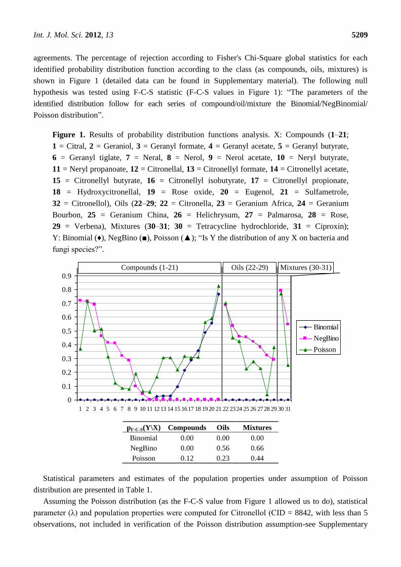
agreements. The percentage of rejection according to Fisher's Chi-Square global statistics for each

identified probability distribution function according to the class (as compounds, oils, mixtures) is

shown in Figure 1 (detailed data can be found in Supplementary material). The following null

hypothesis was tested using F-C-S statistic (F-C-S values in Figure 1): ―The parameters of the

identified distribution follow for each series of compound/oil/mixture the Binomial/NegBinomial/

Poisson distribution‖.

Figure 1. Results of probability distribution functions analysis. X: Compounds (1–21;

1 = Citral, 2 = Geraniol, 3 = Geranyl formate, 4 = Geranyl acetate, 5 = Geranyl butyrate,

6 = Geranyl tiglate, 7 = Neral, 8 = Nerol, 9 = Nerol acetate, 10 = Neryl butyrate,

11 = Neryl propanoate, 12 = Citronellal, 13 = Citronellyl formate, 14 = Citronellyl acetate,

15 = Citronellyl butyrate, 16 = Citronellyl isobutyrate, 17 = Citronellyl propionate,

18 = Hydroxycitronellal, 19 = Rose oxide, 20 = Eugenol, 21 = Sulfametrole,

32 = Citronellol), Oils (22–29; 22 = Citronella, 23 = Geranium Africa, 24 = Geranium

Bourbon, 25 = Geranium China, 26 = Helichrysum, 27 = Palmarosa, 28 = Rose,

29 = Verbena), Mixtures (30–31; 30 = Tetracycline hydrochloride, 31 = Ciproxin);

Y: Binomial (♦), NegBino (■), Poisson (▲); ―Is Y the distribution of any X on bacteria and

fungi species?‖.

0

0.1

0.2

0.3

0.4

0.5

0.6

0.7

0.8

0.9

1 2 3 4 5 6 7 8 9 10 11 1213 14 15 1617 18 1920 21 22 2324 25 26 2728 29 30 31

Binomial

NegBino

Poisson

Compounds (1-21) Oils (22-29) Mixtures (30-31)

pF-C-S(Y\X) Compounds Oils Mixtures

Binomial 0.00 0.00 0.00

NegBino 0.00 0.56 0.66

Poisson 0.12 0.23 0.44

Statistical parameters and estimates of the population properties under assumption of Poisson

distribution are presented in Table 1.

Assuming the Poisson distribution (as the F-C-S value from Figure 1 allowed us to do), statistical

parameter (λ) and population properties were computed for Citronellol (CID = 8842, with less than 5

observations, not included in verification of the Poisson distribution assumption-see Supplementary

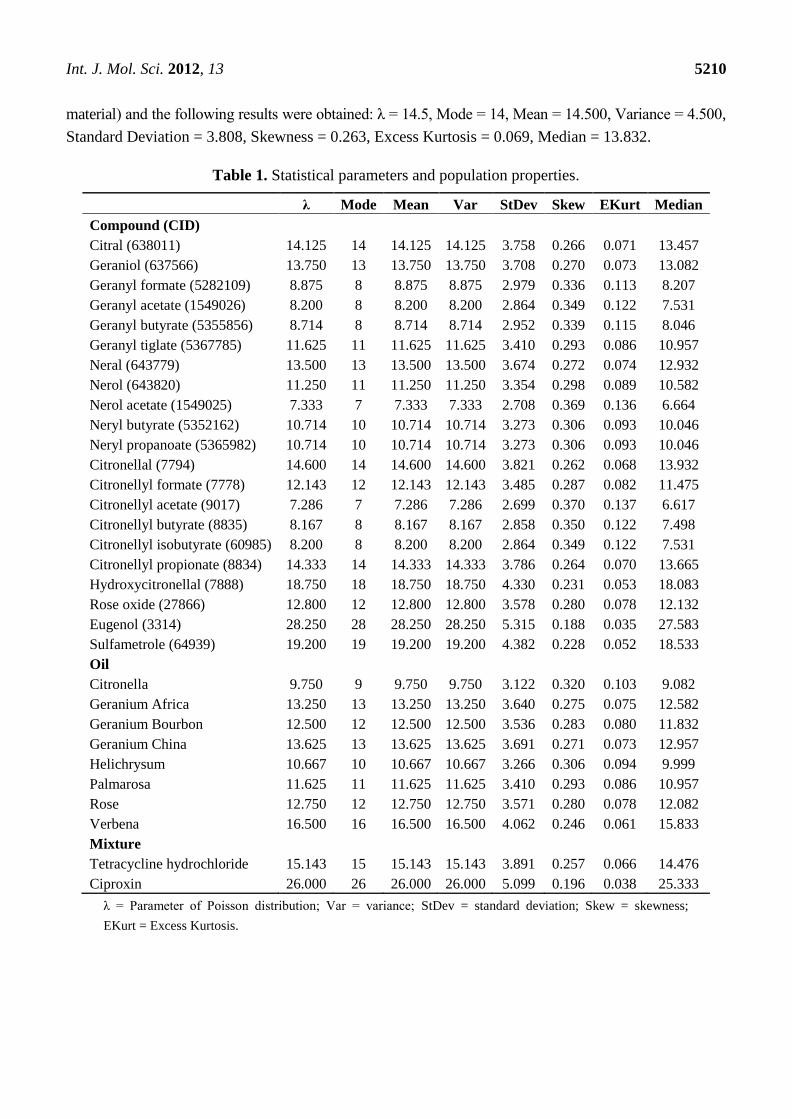
Int. J. Mol. Sci. 2012, 13 5210

material) and the following results were obtained: λ = 14.5, Mode = 14, Mean = 14.500, Variance = 4.500,

Standard Deviation = 3.808, Skewness = 0.263, Excess Kurtosis = 0.069, Median = 13.832.

Table 1. Statistical parameters and population properties.

λ Mode Mean Var StDev Skew EKurt Median

Compound (CID)

Citral (638011) 14.125 14 14.125 14.125 3.758 0.266 0.071 13.457

Geraniol (637566) 13.750 13 13.750 13.750 3.708 0.270 0.073 13.082

Geranyl formate (5282109) 8.875 8 8.875 8.875 2.979 0.336 0.113 8.207

Geranyl acetate (1549026) 8.200 8 8.200 8.200 2.864 0.349 0.122 7.531

Geranyl butyrate (5355856) 8.714 8 8.714 8.714 2.952 0.339 0.115 8.046

Geranyl tiglate (5367785) 11.625 11 11.625 11.625 3.410 0.293 0.086 10.957

Neral (643779) 13.500 13 13.500 13.500 3.674 0.272 0.074 12.932

Nerol (643820) 11.250 11 11.250 11.250 3.354 0.298 0.089 10.582

Nerol acetate (1549025) 7.333 7 7.333 7.333 2.708 0.369 0.136 6.664

Neryl butyrate (5352162) 10.714 10 10.714 10.714 3.273 0.306 0.093 10.046

Neryl propanoate (5365982) 10.714 10 10.714 10.714 3.273 0.306 0.093 10.046

Citronellal (7794) 14.600 14 14.600 14.600 3.821 0.262 0.068 13.932

Citronellyl formate (7778) 12.143 12 12.143 12.143 3.485 0.287 0.082 11.475

Citronellyl acetate (9017) 7.286 7 7.286 7.286 2.699 0.370 0.137 6.617

Citronellyl butyrate (8835) 8.167 8 8.167 8.167 2.858 0.350 0.122 7.498

Citronellyl isobutyrate (60985) 8.200 8 8.200 8.200 2.864 0.349 0.122 7.531

Citronellyl propionate (8834) 14.333 14 14.333 14.333 3.786 0.264 0.070 13.665

Hydroxycitronellal (7888) 18.750 18 18.750 18.750 4.330 0.231 0.053 18.083

Rose oxide (27866) 12.800 12 12.800 12.800 3.578 0.280 0.078 12.132

Eugenol (3314) 28.250 28 28.250 28.250 5.315 0.188 0.035 27.583

Sulfametrole (64939) 19.200 19 19.200 19.200 4.382 0.228 0.052 18.533

Oil

Citronella 9.750 9 9.750 9.750 3.122 0.320 0.103 9.082

Geranium Africa 13.250 13 13.250 13.250 3.640 0.275 0.075 12.582

Geranium Bourbon 12.500 12 12.500 12.500 3.536 0.283 0.080 11.832

Geranium China 13.625 13 13.625 13.625 3.691 0.271 0.073 12.957

Helichrysum 10.667 10 10.667 10.667 3.266 0.306 0.094 9.999

Palmarosa 11.625 11 11.625 11.625 3.410 0.293 0.086 10.957

Rose 12.750 12 12.750 12.750 3.571 0.280 0.078 12.082

Verbena 16.500 16 16.500 16.500 4.062 0.246 0.061 15.833

Mixture

Tetracycline hydrochloride 15.143 15 15.143 15.143 3.891 0.257 0.066 14.476

Ciproxin 26.000 26 26.000 26.000 5.099 0.196 0.038 25.333

λ = Parameter of Poisson distribution; Var = variance; StDev = standard deviation; Skew = skewness;

EKurt = Excess Kurtosis.

Int. J. Mol. Sci. 2012, 13 5211

2.2. QSAR Models

Two requirements were imposed in identification of the proper transformation of Poisson parameter

λ: the absence of outliers and the presence of normality at a significance level of 5%. The global F-C-S

distribution statistic indicated that the Poisson parameter more likely follows a Log-normal distribution

(statistics: K−S = 0.1315; pK−S = 0.7948; A−D = 0.3874; CritA−D5% = 2.5018 (critical values associated

for Anderson-Darling test); C−Sdf = 2 = 0.9403; pC−S = 0.6249).

The Eugenol compound was identified as outlier with Grubbs' test (Z = 3.178, Zcritical−5% = 2.7338).

After natural logarithm transformation of the Poisson parameters, seen as an overall antimicrobial

activity of investigated compounds, no other outlier was identified (the highest Z value was of 2.528;

Zcritical−5% = 2.758) and the normality hypothesis of the ln(λ) values could not be rejected (p > 0.05).

Further testing on ln(λ) under the normal distribution assumption gave no reason to reject the normality

of the data in the training test (K−S = 0.14351, pK−S = 0.917; A−D = 0.37751, pA−D = 0.686;

C−S = 0.62246, pC−S = 0.430; F−C−S = 1.307; pF−C−S = 0.727) nor in test set (K−S = 0.2301, pK−S = 0.779;

A−D = 0.3860, pA−D = 0.679; F−C−S = 0.637; pF−C−S = 0.727).

2.2.1. Based on DRAGON Descriptors

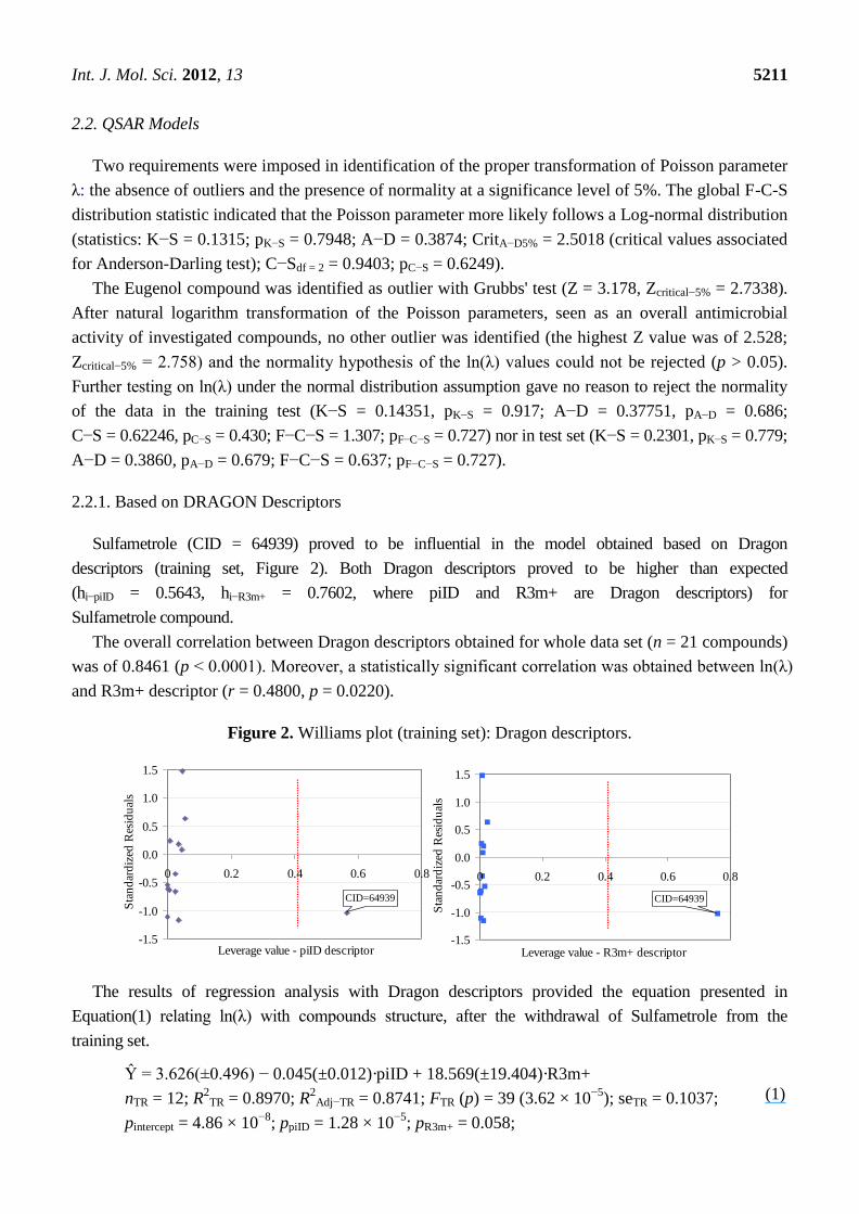
Sulfametrole (CID = 64939) proved to be influential in the model obtained based on Dragon

descriptors (training set, Figure 2). Both Dragon descriptors proved to be higher than expected

(hi−piID = 0.5643, hi−R3m+ = 0.7602, where piID and R3m+ are Dragon descriptors) for

Sulfametrole compound.

The overall correlation between Dragon descriptors obtained for whole data set (n = 21 compounds)

was of 0.8461 (p < 0.0001). Moreover, a statistically significant correlation was obtained between ln(λ)

and R3m+ descriptor (r = 0.4800, p = 0.0220).

Figure 2. Williams plot (training set): Dragon descriptors.

-1.5

-1.0

-0.5

0.0

0.5

1.0

1.5

0 0.2 0.4 0.6 0.8

Leverage value - piID descriptor

Sta

nd

ard

ized

Res

idu

als

CID=64939

-1.5

-1.0

-0.5

0.0

0.5

1.0

1.5

0 0.2 0.4 0.6 0.8

Leverage value - R3m+ descriptor

Sta

nd

ard

ized

Res

idu

als

CID=64939

The results of regression analysis with Dragon descriptors provided the equation presented in

Equation(1) relating ln(λ) with compounds structure, after the withdrawal of Sulfametrole from the

training set.

Ŷ = 3.626(±0.496) − 0.045(±0.012)·piID + 18.569(±19.404)·R3m+

nTR = 12; R2

TR = 0.8970; R2

Adj−TR = 0.8741; FTR (p) = 39 (3.62 × 10−5

); seTR = 0.1037;

pintercept = 4.86 × 10−8

; ppiID = 1.28 × 10−5

; pR3m+ = 0.058;

(1)

Int. J. Mol. Sci. 2012, 13 5212

TpiID = TR3m+ = 0.776; VIFpiID = VIFR3m+ = 1.305;

R(Y−piID)TR = −0.9183 (p-value = 2.50 × 10−5

); R(Y−R3m+)TR = −0.2410 (p-value = 0.4505);

R(piID−R3m+)TR = 0.4833 (p-value = 0.1114);

R2

loo = 0.8452; Floo (p) = 24 (2.35 × 10−4

); seloo = 0.1276;

nTS = 7; R2

TS = 0.6518; FTS (p) = 11 (2.16 × 10−2

);

R(Y−piID)TS = −0.0869 (p-value = 0.8241); R(Y−R3m+)TS = −0.2410 (p-value = 0.0024);

R(piID−R3m+)TS = 0.3469 (p-value = 0.3604)

where Ŷ = ln(λ) estimated by Equation(1); R2 = determination coefficient; TR = training set;

loo = leave-one-out analysis; TS = test set; Ext = external set; R2

Adj = adjusted determination

coefficient; F = F-value (from ANOVA table); p = p-value associated to F-value; se = standard error

of estimate; Dragon descriptors: piID = conventional bond order ID number-walk and path counts;

R3m+ = R maximal autocorrelation of lag 3/weighted by mass GETAWAY descriptors;

T = Tolerance; VIF = Variance Inflation Factor; R = correlation coefficient.

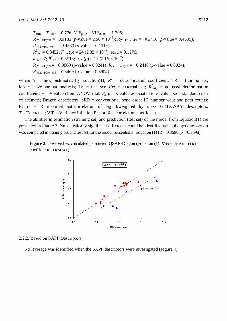
The abilities in estimation (training set) and prediction (test set) of the model from Equation(1) are

presented in Figure 3. No statistically significant difference could be identified when the goodness-of-fit

was compared in training set and test set for the model presented in Equation (1) (Z = 0.3590, p = 0.3598).

Figure 3. Observed vs. calculated parameter: QSAR-Dragon (Equation (1), R2TS = determination

coefficient in test set).

2.2.2. Based on SAPF Descriptors

No leverage was identified when the SAPF descriptors were investigated (Figure 4).

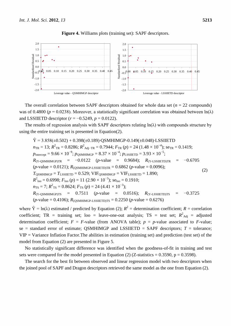
Int. J. Mol. Sci. 2012, 13 5213

Figure 4. Williams plots (training set): SAPF descriptors.

-2.0

-1.5

-1.0

-0.5

0.0

0.5

1.0

1.5

2.0

0.00 0.05 0.10 0.15 0.20 0.25 0.30 0.35 0.40 0.45

Leverage value - QSMHIMGP descriptor

Sta

nd

ard

ized

Res

idu

als

-2.0

-1.5

-1.0

-0.5

0.0

0.5

1.0

1.5

2.0

0.00 0.05 0.10 0.15 0.20 0.25 0.30 0.35 0.40 0.45

Leverage value - LSSIIETD descriptor

Sta

ndar

diz

ed R

esid

ual

s

The overall correlation between SAPF descriptors obtained for whole data set (n = 22 compounds)

was of 0.4800 (p = 0.0238). Moreover, a statistically significant correlation was obtained between ln(λ)

and LSSIIETD descriptor (r = −0.5249, p = 0.0122).

The results of regression analysis with SAPF descriptors relating ln(λ) with compounds structure by

using the entire training set is presented in Equation(2).

Ŷ = 3.858(±0.502) + 0.398(±0.189)·QSMHIMGP-0.149(±0.048)·LSSIIETD

nTR = 13; R2

TR = 0.8286; R2

Adj−TR = 0.7944; FTR (p) = 24 (1.48 × 10−4

); seTR = 0.1419;

pintercept = 9.66 × 10−9

; pQSMHIMGP = 8.37 × 10−4

; pLSSIIETD = 3.93 × 10−5

;

R(Y-QSMHIMGP)TR = −0.0122 (p-value = 0.9684); R(Y-LSSIIETD)TR = −0.6705

(p-value = 0.0121); R(QSMHIMGP-LSSIIETD)TR = 0.6862 (p-value = 0.0096);

TQSMHIMGP = TLSSIIETD = 0.529; VIFQSMHIMGP = VIFLSSIIETD = 1.890;

R2

loo = 0.6998; Floo (p) = 11 (2.90 × 10−3

); seloo = 0.1910;

nTS = 7; R2

TS = 0.8624; FTS (p) = 24 (4.41 × 10−3

);

R(Y-QSMHIMGP)TS = 0.7511 (p-value = 0.0516); R(Y-LSSIIETD)TS = −0.3725

(p-value = 0.4106); R(QSMHIMGP-LSSIIETD)TS = 0.2250 (p-value = 0.6276)

(2)

where Ŷ = ln(λ) estimated / predicted by Equation (2); R2 = determination coefficient; R = correlation

coefficient; TR = training set; loo = leave-one-out analysis; TS = test set; R2

Adj = adjusted

determination coefficient; F = F-value (from ANOVA table); p = p-value associated to F-value;

se = standard error of estimate; QSMHIMGP and LSSIIETD = SAPF descriptors; T = tolerance;

VIP = Variance Inflation Factor.The abilities in estimation (training set) and prediction (test set) of the

model from Equation (2) are presented in Figure 5.

No statistically significant difference was identified when the goodness-of-fit in training and test

sets were compared for the model presented in Equation (2) (Z-statistics = 0.3590, p = 0.3598).

The search for the best fit between observed and linear regression model with two descriptors when

the joined pool of SAPF and Dragon descriptors retrieved the same model as the one from Equation (2).

Int. J. Mol. Sci. 2012, 13 5214

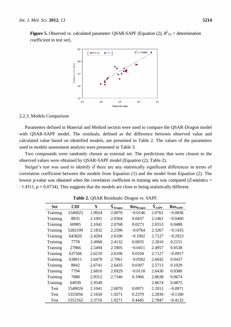
Figure 5. Observed vs. calculated parameter: QSAR-SAPF (Equation (2), R2TS = determination

coefficient in test set).

2.2.3. Models Comparison

Parameters defined in Material and Method section were used to compare the QSAR-Dragon model

with QSAR-SAPF model. The residuals, defined as the difference between observed value and

calculated value based on identified models, are presented in Table 2. The values of the parameters

used in models assessment analysis were presented in Table 3.

Two compounds were randomly chosen as external set. The predictions that were closest to the

observed values were obtained by QSAR-SAPF model (Equation (2); Table 2).

Steiger’s test was used to identify if there are any statistically significant differences in terms of

correlation coefficient between the models from Equation (1) and the model from Equation (2). The

lowest p-value was obtained when the correlation coefficient in training sets was compared (Z-statistics =

−1.4511, p = 0.0734). This suggests that the models are close to being statistically different.

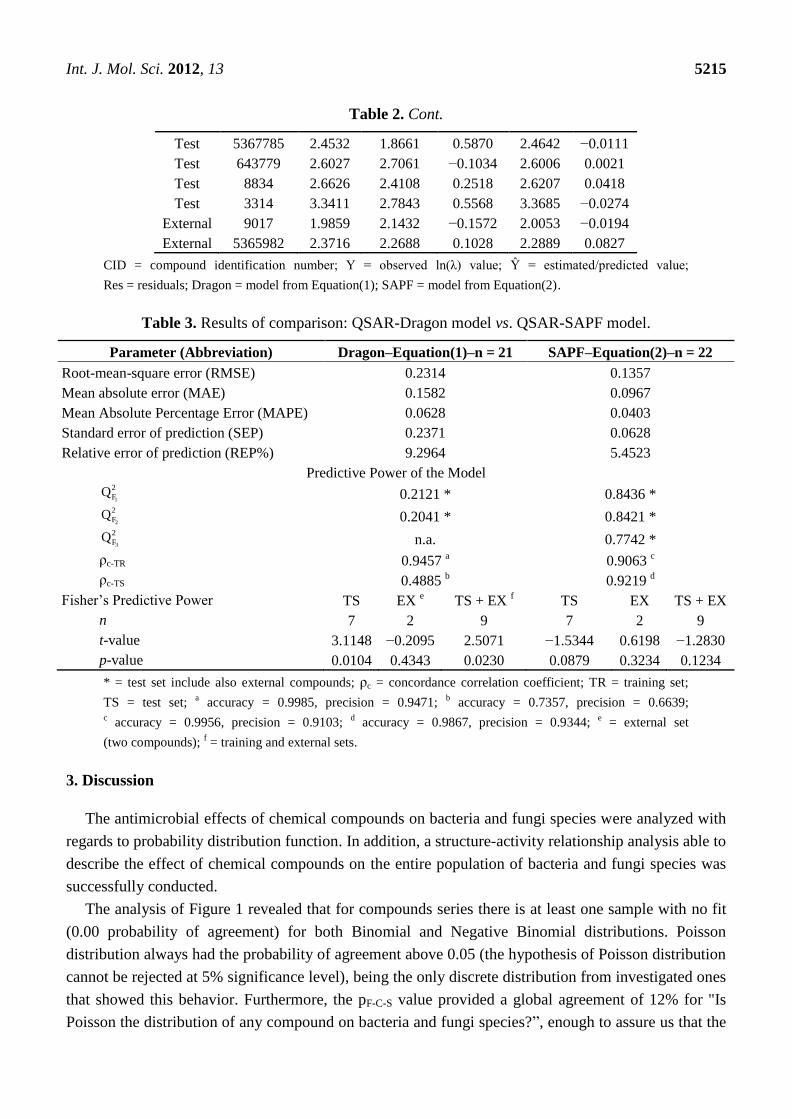
Table 2. QSAR Residuals: Dragon vs. SAPF.

Set CID Y ŶDragon ResDragon ŶSAPF ResSAPF

Training 1549025 1.9924 2.0070 −0.0146 2.0761 −0.0836

Training 8835 2.1001 2.0564 0.0437 2.1461 −0.0460

Training 60985 2.1041 2.0768 0.0273 2.0553 0.0488

Training 5282109 2.1832 2.2596 −0.0764 2.3267 −0.1435

Training 643820 2.4204 2.6106 −0.1902 2.7127 −0.2923

Training 7778 2.4968 2.4132 0.0835 2.2816 0.2151

Training 27866 2.5494 2.5905 −0.0411 2.4957 0.0538

Training 637566 2.6210 2.6106 0.0104 2.7127 −0.0917

Training 638011 2.6479 2.7061 −0.0582 2.6042 0.0437

Training 8842 2.6741 2.6435 0.0307 2.5713 0.1029

Training 7794 2.6810 2.6929 −0.0118 2.6430 0.0380

Training 7888 2.9312 2.7346 0.1966 2.8638 0.0674

Training 64939 2.9549 2.8674 0.0875

Test 1549026 2.1041 2.0070 0.0971 2.2012 −0.0971

Test 5355856 2.1650 1.9271 0.2379 2.2830 −0.1180

Test 5352162 2.3716 1.9271 0.4445 2.7847 −0.4132

Int. J. Mol. Sci. 2012, 13 5215

Table 2. Cont.

Test 5367785 2.4532 1.8661 0.5870 2.4642 −0.0111

Test 643779 2.6027 2.7061 −0.1034 2.6006 0.0021

Test 8834 2.6626 2.4108 0.2518 2.6207 0.0418

Test 3314 3.3411 2.7843 0.5568 3.3685 −0.0274

External 9017 1.9859 2.1432 −0.1572 2.0053 −0.0194

External 5365982 2.3716 2.2688 0.1028 2.2889 0.0827

CID = compound identification number; Y = observed ln(λ) value; Ŷ = estimated/predicted value;

Res = residuals; Dragon = model from Equation(1); SAPF = model from Equation(2).

Table 3. Results of comparison: QSAR-Dragon model vs. QSAR-SAPF model.

Parameter (Abbreviation) Dragon–Equation(1)–n = 21 SAPF–Equation(2)–n = 22

Root-mean-square error (RMSE) 0.2314 0.1357

Mean absolute error (MAE) 0.1582 0.0967

Mean Absolute Percentage Error (MAPE) 0.0628 0.0403

Standard error of prediction (SEP) 0.2371 0.0628

Relative error of prediction (REP%) 9.2964 5.4523

Predictive Power of the Model 2

F1Q 0.2121 *

0.8436 *

2

F2Q 0.2041 * 0.8421 *

2

F3Q n.a. 0.7742 *

ρc-TR 0.9457 a 0.9063

c

ρc-TS 0.4885 b 0.9219

d

Fisher’s Predictive Power TS EX e

TS + EX f

TS EX TS + EX

n 7 2 9 7 2 9

t-value 3.1148 −0.2095 2.5071 −1.5344 0.6198 −1.2830

p-value 0.0104 0.4343 0.0230 0.0879 0.3234 0.1234

* = test set include also external compounds; ρc = concordance correlation coefficient; TR = training set;

TS = test set; a accuracy = 0.9985, precision = 0.9471;

b accuracy = 0.7357, precision = 0.6639;

c accuracy = 0.9956, precision = 0.9103;

d accuracy = 0.9867, precision = 0.9344;

e = external set

(two compounds); f = training and external sets.

3. Discussion

The antimicrobial effects of chemical compounds on bacteria and fungi species were analyzed with

regards to probability distribution function. In addition, a structure-activity relationship analysis able to

describe the effect of chemical compounds on the entire population of bacteria and fungi species was

successfully conducted.

The analysis of Figure 1 revealed that for compounds series there is at least one sample with no fit

(0.00 probability of agreement) for both Binomial and Negative Binomial distributions. Poisson

distribution always had the probability of agreement above 0.05 (the hypothesis of Poisson distribution

cannot be rejected at 5% significance level), being the only discrete distribution from investigated ones

that showed this behavior. Furthermore, the pF-C-S value provided a global agreement of 12% for "Is

Poisson the distribution of any compound on bacteria and fungi species?‖, enough to assure us that the

Int. J. Mol. Sci. 2012, 13 5216

Poisson distribution is the true distribution of compounds’ antimicrobial activities on the studied

bacteria and fungi species. The situation is somehow reversed for oils and mixtures; if the Poisson

distribution is the only one not rejected for compounds, then the Negative Binomial distribution also

cannot be rejected for oils and mixtures. A deeper investigation on factors influencing antimicrobial

activities may reveal that the negative binomial distribution should be rejected for the whole data

presented in Table 4. The reason for this fact should be foundd in the distribution of the compounds

series activities on a given bacteria (columns data in Table 4).

Thus, it was already proven [34] that Negative Binomial distribution occurs when both column and

row data are shaped by Poisson distribution, which is not our case since only rows (a compound

activity) are shaped by Poisson distribution (see Figure 1). Moreover, rows data from Table 4 are more

likely to be Negative Binomial distributed, suggesting that at least two factors coexist in the

compounds’ structure and influence their activity.

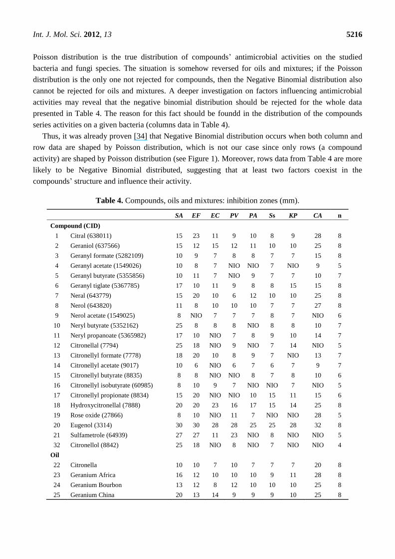
Table 4. Compounds, oils and mixtures: inhibition zones (mm).

SA EF EC PV PA Ss KP CA n

Compound (CID)

1 Citral (638011) 15 23 11 9 10 8 9 28 8

2 Geraniol (637566) 15 12 15 12 11 10 10 25 8

3 Geranyl formate (5282109) 10 9 7 8 8 7 7 15 8

4 Geranyl acetate (1549026) 10 8 7 NIO NIO 7 NIO 9 5

5 Geranyl butyrate (5355856) 10 11 7 NIO 9 7 7 10 7

6 Geranyl tiglate (5367785) 17 10 11 9 8 8 15 15 8

7 Neral (643779) 15 20 10 6 12 10 10 25 8

8 Nerol (643820) 11 8 10 10 10 7 7 27 8

9 Nerol acetate (1549025) 8 NIO 7 7 7 8 7 NIO 6

10 Neryl butyrate (5352162) 25 8 8 8 NIO 8 8 10 7

11 Neryl propanoate (5365982) 17 10 NIO 7 8 9 10 14 7

12 Citronellal (7794) 25 18 NIO 9 NIO 7 14 NIO 5

13 Citronellyl formate (7778) 18 20 10 8 9 7 NIO 13 7

14 Citronellyl acetate (9017) 10 6 NIO 6 7 6 7 9 7

15 Citronellyl butyrate (8835) 8 8 NIO NIO 8 7 8 10 6

16 Citronellyl isobutyrate (60985) 8 10 9 7 NIO NIO 7 NIO 5

17 Citronellyl propionate (8834) 15 20 NIO NIO 10 15 11 15 6

18 Hydroxycitronellal (7888) 20 20 23 16 17 15 14 25 8

19 Rose oxide (27866) 8 10 NIO 11 7 NIO NIO 28 5

20 Eugenol (3314) 30 30 28 28 25 25 28 32 8

21 Sulfametrole (64939) 27 27 11 23 NIO 8 NIO NIO 5

32 Citronellol (8842) 25 18 NIO 8 NIO 7 NIO NIO 4

Oil

22 Citronella 10 10 7 10 7 7 7 20 8

23 Geranium Africa 16 12 10 10 10 9 11 28 8

24 Geranium Bourbon 13 12 8 12 10 10 10 25 8

25 Geranium China 20 13 14 9 9 9 10 25 8

Int. J. Mol. Sci. 2012, 13 5217

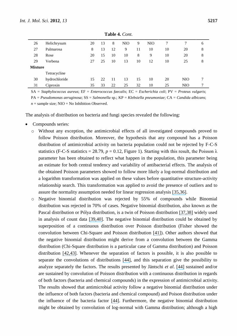
Table 4. Cont.

26 Helichrysum 20 13 8 NIO 9 NIO 7 7 6

27 Palmarosa 8 13 12 9 11 10 10 20 8

28 Rose 20 15 10 10 8 9 10 20 8

29 Verbena 27 25 10 13 10 12 10 25 8

Mixture

30

Tetracycline

hydrochloride 15 22 11 13 15 10 20 NIO 7

31 Ciproxin 35 33 22 25 32 10 25 NIO 7

SA = Staphylococcus aureus; EF = Enterococcus faecalis; EC = Escherichia coli; PV = Proteus vulgaris;

PA = Pseudomonas aeruginosa; SS = Salmonella sp.; KP = Klebsiella pneumoniae; CA = Candida albicans;

n = sample size; NIO = No Inhibition Observed.

The analysis of distribution on bacteria and fungi species revealed the following:

Compounds series:

o Without any exception, the antimicrobial effects of all investigated compounds proved to

follow Poisson distribution. Moreover, the hypothesis that any compound has a Poisson

distribution of antimicrobial activity on bacteria population could not be rejected by F-C-S

statistics (F-C-S statistics = 28.79, p = 0.12, Figure 1). Starting with this result, the Poisson λ

parameter has been obtained to reflect what happen in the population, this parameter being

an estimate for both central tendency and variability of antibacterial effects. The analysis of

the obtained Poisson parameters showed to follow more likely a log-normal distribution and

a logarithm transformation was applied on these values before quantitative structure-activity

relationship search. This transformation was applied to avoid the presence of outliers and to

assure the normality assumption needed for linear regression analysis [35,36].

o Negative binomial distribution was rejected by 55% of compounds while Binomial

distribution was rejected in 70% of cases. Negative binomial distribution, also known as the

Pascal distribution or Pólya distribution, is a twin of Poisson distribution [37,38] widely used

in analysis of count data [39,40]. The negative binomial distribution could be obtained by

superposition of a continuous distribution over Poisson distribution (Fisher showed the

convolution between Chi-Square and Poisson distribution [41]). Other authors showed that

the negative binomial distribution might derive from a convolution between the Gamma

distribution (Chi-Square distribution is a particular case of Gamma distribution) and Poisson

distribution [42,43]. Whenever the separation of factors is possible, it is also possible to

separate the convolutions of distributions [44], and this separation give the possibility to

analyze separately the factors. The results presented by Jäntschi et al. [44] sustained and/or

are sustained by convolution of Poisson distribution with a continuous distribution in regards

of both factors (bacteria and chemical compounds) in the expression of antimicrobial activity.

The results showed that antimicrobial activity follow a negative binomial distribution under

the influence of both factors (bacteria and chemical compound) and Poison distribution under

the influence of the bacteria factor [44]. Furthermore, the negative binomial distribution

might be obtained by convolution of log-normal with Gamma distribution; although a high

Int. J. Mol. Sci. 2012, 13 5218

number of observations are needed (n > 250) in order to statistically assure the difference

between Log-normal and Gamma distributions [45].

Oils and mixture series:

o Negative Binomial distribution cannot be rejected for oils. Moreover, Negative Binomial

distribution for oils had a higher likelihood than Poisson distribution (pF-C-S for Negative

Binomial: 0.56; pF-C-S for Poisson: 0.23) while the Binomial distribution was rejected.

o Negative Binomial distribution cannot be rejected for mixtures either. Moreover, Negative

Binomial distribution for mixtures had also higher likelihood than Poisson distribution (pF-C-S for

Negative Binomial = 0.66; pF-C-S for Poisson = 0.44) while the Binomial distribution was rejected.

o The above-presented facts suggest that in the case of oils and mixtures, the factors of the

antibacterial activity are not completely separated when oil/mixture name are taken as factor;

this appears to be because the Negative Binomial distribution often occurs when a

convolution/superposition of Poisson distributions characterize the observed data [46].

Overall, any investigated compound, oil and mixture proved to have an antimicrobial effect that

follows the Poisson distribution on studied bacteria and fungi species. The λ Poisson parameter, varied

from 7.286 (Nerol acetate) to 28.250 (Eugenol) and represents the mean and variance of inhibition

zone of compound/oil/mixture on investigated species. The obtained parameter of Poisson distribution

proved able to characterize the overall antimicrobial activity (both mean and variance equals to

Poisson parameter λ, Table 1) of the compounds on the investigated bacteria population.

The structure-activity relationships between compounds’ structure and the overall antimicrobial effect

on bacteria population, as well as the suitability of a pool of descriptors (SAPF and Dragon approaches)

for the overall antimicrobial activity estimation and prediction were furthermore investigated.

QSAR model with two descriptors that proved abilities in estimation and prediction was identified

for each approach after the split of compounds in training (13 compounds), test (7 compounds) and

external (2 compounds) sets. Normal distribution of the observations was assured through natural

logarithm transformation (p > 0.05) to allow investigation of structure (of compounds)-activity (overall

antimicrobial activity) relationships using multiple linear regression.

The analysis of QSAR-Dragon model revealed the following:

One compound proved to be influential in the model (CID = 64939, Figure 2). This compound

obtained the value of leverage for both Dragon descriptors higher than the accepted threshold

(0.41). This compound, which belongs to the training set, was withdrawn, and a model based

on 12 compounds in training set was obtained, Equation(1).

Two descriptors were able to describe the linear relation between overall antimicrobial activities

of investigated compounds. One descriptor belongs to the walk and path counts and relates the

conventional bond order ID number while the second descriptor relates the maximal

autocorrelation of lag 3 divided by mass (R3m+). According with associated coefficients, the

R3m+ had a higher contribution in the model compared with piID descriptor, but its contribution

is to the significance level threshold (5.8% compared to imposed 5% significance level).

QSAR-Dragon model proved to be statistically significant (F = 39, p = 3.62 × 10−5

). A low

value of root mean square error was obtained in leave-one-out analysis (0.1276). The

contribution of R3m+ descriptor to the model is questionable since the significance associated

Int. J. Mol. Sci. 2012, 13 5219

to its coefficient is very close to 0.05 but since it has a real contribution in the r2 value its

significance of 5.8% was accepted. Moreover, the R3m+ proved not significantly correlate with

Poisson parameter (r = −0.2410).

Multicollianearity is not present in the model since the tolerance value 0.1 < T < 1 and the

variance inflation factors (VIF) < 10 even if a significant correlation coefficient was obtained

between Dragon descriptors.

The model proved its abilities in estimation (R2

TR = 0.897) as well as in prediction (internal

validity of the model in leave-one-out analysis, R2

loo = 0.845 and external validation in test set

R2

TS = 0.652) with a difference in the goodness-of-fit from 0.052 (training vs. interval

validation - leave one out analysis) to 0.245 (training vs. external validation-test set). However,

the difference of 0.245 proved not statistically significant (p > 0.05).

Unfortunately, external abilities in prediction were away from the expected abilities. The trend

is significant far from the expected line-Figure 3.

The abilities in estimation (training set) proved not statistically significant from the abilities in

prediction (test set) since a probability of 0.3598 was obtained in comparison.

The analysis of QSAR-SAPF model revealed the following:

The values of SAPF descriptors associated to compounds proved that no compound had

significant influence on the model (all leverage values where lower than threshold −0.41, Figure 4).

SAPF model proved statistically significant (F = 24, p = 1.48 × 10−4

). The contribution of both

descriptors to the model proved statistically significant (p-values associated to coefficients <0.05).

According to descriptors from Equation(2), the global model of antibacterial activity is related to

both molecular geometry and topology: one descriptor identified a relation between the geometry

of compounds and the overall antimicrobial activity while the second descriptor identified a

relation with compounds’ topology. Moreover, the atomic mass and electronegativity proved to

be related to the overall antimicrobial activity by the same split ratio in the expression of the

model descriptors.

Multicollianearity was not identified in the QSAR-SAPF model, even if a statistically significant

correlation coefficient between descriptors exists (the tolerance values were higher than 0.1 and

smaller than 1 and the variance inflation factors (VIF) had values smaller than 10).

The model proved its abilities in estimation (R2TR = 0.829) as well as in prediction (internal

validity of the model in leave-one-out analysis, R2

loo = 0.700 and external validation in test set

R2TS = 0.862) with a difference in the goodness-of-fit from −0.034 (training vs. external

validation - test set) to 0.129 (training vs. interval validation-leave one out analysis). Moreover,

none of these differences were statistically significant (p > 0.05).

External abilities in prediction proved to be close to expected abilities for QSAR-SAPF model (Figure 5).

The comparison of the identified models revealed the following:

Dragon model has slightly better abilities in estimation compared to SAPF model, but these

abilities proved not statistically significant. The determination coefficient obtained both in

training set and in leave-one-out analysis was higher compared to SAPF model with 0.068 and

respectively 0.145. Moreover, the abilities of prediction seem to be better for SAPF model

Int. J. Mol. Sci. 2012, 13 5220

compared to Dragon model (a difference of 0.211, not statistically significant p < 0.05). This

observation is also sustained by the lowest value of residuals in training set for Dragon model and

in two compounds from training set and all compounds from test set for SAPF model (Table 2).

The SAPF model systematically obtained smallest values of parameters presented in Table 3: best

explaining the variability in the observation; smallest typical errors; smallest standard error of

prediction as well as smallest relative error of prediction. The highest difference is observed with

regards to standard error of prediction that is almost 4 times higher for Dragon model compared

to SAPF model.

The analysis of predictive power of the models demonstrated that SAPF model had significantly

higher power of prediction (Table 3). According to the obtained results, the Q2 values for Dragon

model are smaller than 0.6, being considered unacceptable while all Q2 values for SAPF model

are higher than 0.77. These results show that the Dragon model can be rejected from a statistical

point of view, taking also into consideration that the relative error of prediction is almost 2 times

higher compared to SAPF model.

Furthermore, the mean of residuals for training, external and external + test set proved not

statistically different by zero when the SAPF model was analyzed. The Fisher’s predictive power

identified statistically difference by zero of the residuals obtained by Dragon model in both

training and test sets (9 compounds) (p < 0.05, Table 3).

The model with a higher concordance between observed and estimated/predicted could be considered

the best model. The analysis of concordance correlation coefficient revealed a substantial strength of

agreement for training set but a very poor agreement in test set for Dragon model. A moderate

strength of agreement was obtained by SAPF model in both training and test sets (Table 3).

Steiger’s test was not able to identify any statistically significant differences between Dragon

and SAPF model regarding goodness-of-fit neither in training set nor in external set.

It can be concluded based on the facts presented above that the SAPF model is a reliable, valid

(internally as well as externally) and stable model useful in characterization of overall antimicrobial

activity on investigated compounds, both in terms of estimation and prediction.

The aim and objectives of the research have been achieved. The antimicrobial effect proved to

follow the Poisson distribution and its parameter was furthermore used to identify those descriptors

from Dragon and SAPF pools able to characterize the link between compounds and overall

antimicrobial activity. Two newly developed models were found statistically valid. However, which of

these QSAR models is better? The analysis of applicability domain of the models obtained in training

sets was able to identify based on the values of descriptors one structurally influential compound in

training set for Dragon model. According to the obtained results, one compound was withdrawn from

further analysis in Dragon modeling. Dragon model was created based on 12 compounds in training set

while the SAPF model was created based on 13 compounds in training set. Graphical representation of

observed vs. calculated values based on identified models as well as the predictive power parameters

showed that the best model to be applied on new chemicals is the SAPF model.

Int. J. Mol. Sci. 2012, 13 5221

4. Experimental Section

4.1. Compounds, Oils and Mixtures

The antimicrobial effects of twenty-two compounds, eight oils and two mixtures on gram-positive

and -negative bacteria (Staphylococcus aureus, Enterococcus faecalis, Escherichia coli, Pseudomonas

aeruginosa, Klebsiella pneumoniae, Proteus vulgaris, Salmonella sp.) and on one fungus (Candida

albicans), expressed as inhibition zone (mm, Agar diffusion disc method [33]), were included in the

analysis (Table 4). The PubChem database was used to retrieve the compounds structure and

associated CIDs (Compound IDentification numbers); the data are presented in Table 4.

4.2. Distribution Analysis

Since all inhibition zones expressed in mm are integer numbers, a search for a discrete distribution

was conducted having as alternatives Uniform, Binomial, Negative Binomial and Poisson distributions

(other alternatives were excluded due to lack of fit with observed data). Kolmogorov-Smirnov (K-S) [47]

and Anderson-Darling (A-D) [48] statistics were used to measure the departure between observations

and a certain probability distribution function (PDF). Fisher’s method combining independent tests for

significance (Fisher’s Chi-Square, abbreviated as F-C-S [49]) was used to obtain a global probability

of agreement between the distribution and the observed samples.

The whole pool (matrix) of data was prior analyzed and none of the above distribution functions

give an acceptable (higher than 5%) agreement with the observations. This fact could be explained by

the heterogeneity of the chemicals/oils/mixtures.

In order to obtain the PDF of antimicrobial effects of compounds, oils and mixtures on bacteria and

fungus population, rows of experimental values were analyzed as independent samples. A number of

five observations in sample qualified the sample for estimation of the distribution parameters, and the

analysis was conducted using maximum likelihood estimation (MLE) [34] procedure. The measure of

the agreement was expressed using the probability of F-C-S test. Also the following hypothesis was

tested: a certain PDF can be accepted for populations of all samples regardless of PDF parameters

values. The identified PDF was further used to estimate the population parameter(s) for sample(s)

without enough data (e.g., Citronellol, see Table 4).

Population statistics of the identified PDF can be seen as an estimator of overall antimicrobial

activity of the investigated compound on the bacteria and fungi population. The series of the

population statistics for all investigated compounds was furthermore subject of a structure-activity

relationship search intended to relate the overall antimicrobial effect with compounds’ structure.

4.3. Molecular Descriptors Calculation

The molecular modeling study was conducted at PM3 semi-empirical level of theory [50] on

chemical compounds series.

A series of home-made programs were used to perform the following tasks: ▪ automate transformation

the *.sdf or *.mol files as *.hin files; ▪ prepare the compounds for modeling (run HyperChem v.8.0 [51]

with HyperChem scripts in order to obtain molecular models) [52]; ▪ calculate the molecular descriptors

Int. J. Mol. Sci. 2012, 13 5222

(SAPF approach) for all compounds (calculate all descriptors; select a relevant subset of descriptors);

▪ split the set randomly in training (for model development, ~2/3 compounds in training set) and two test

sets (for model validation); ▪ search for multiple linear regression (search for two descriptors linear

models) in training set; ▪ validate the model obtained in training set on test sets.

The molecular descriptors for the chemical compounds were calculated using a home-made

software that implemented Structural Atomic Property Family [53,54] (SAPF approach, methodology

of calculation depicted in Figure 6) and the Dragon software [55] (all Dragon descriptors).

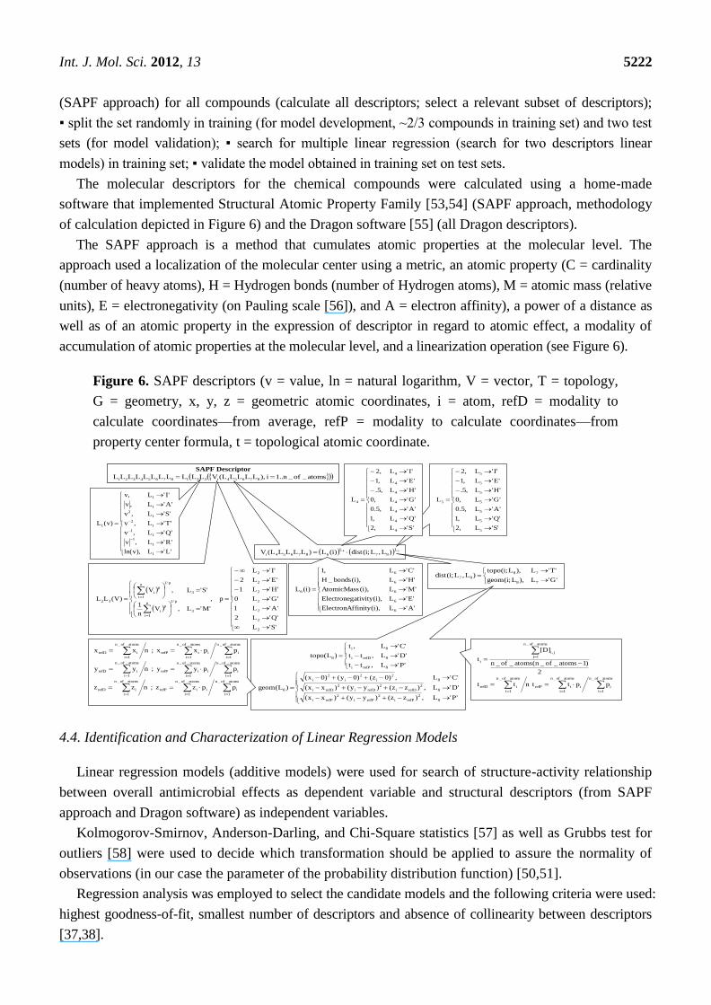
The SAPF approach is a method that cumulates atomic properties at the molecular level. The

approach used a localization of the molecular center using a metric, an atomic property (C = cardinality

(number of heavy atoms), H = Hydrogen bonds (number of Hydrogen atoms), M = atomic mass (relative

units), E = electronegativity (on Pauling scale [56]), and A = electron affinity), a power of a distance as

well as of an atomic property in the expression of descriptor in regard to atomic effect, a modality of

accumulation of atomic properties at the molecular level, and a linearization operation (see Figure 6).

Figure 6. SAPF descriptors (v = value, ln = natural logarithm, V = vector, T = topology,

G = geometry, x, y, z = geometric atomic coordinates, i = atom, refD = modality to

calculate coordinates—from average, refP = modality to calculate coordinates—from

property center formula, t = topological atomic coordinate.

SAPF Descriptor

atoms_of_n..1i),LLLLL(VLLLLLLLLLLL 87654i32187654321

'S'L

'Q'L2

'A'L1

'G'L0

'H'L1

'E'L2

'I'L

p,

'M'L,Vn

1

'S'L,V

)V(LL

2

2

2

2

2

2

2

3

p/1n

1i

p

i

3

p/1n

1i

p

i

32

'L'L),vln(

'R'L,v

'Q'L,v

'T'L,v

'S'L,v

'A'L,v

'I'L,v

)v(L

1

1

11

1

1

2

1

2

1

1

1

54 L

87

L

687654i )L,L;i(dist)i(L)LLLLL(V

'S'L,2

'Q'L,1

'A'L,5.0

'G'L,0

'H'L,5.

'E'L,1

'I'L,2

L

5

5

5

5

5

5

5

5

'G'L),L;i(geom

'T'L),L;i(topo)L,L;i(dist

78

78

87

'S'L,2

'Q'L,1

'A'L,5.0

'G'L,0

'H'L,5.

'E'L,1

'I'L,2

L

4

4

4

4

4

4

4

4

'P'L,tt

'D'L,tt

'C'L,t

)L(topo

8refPi

8refDi

8i

8

'P'L,)zz()yy()xx(

'D'L,)zz()yy()xx(

'C'L,)0z()0y()0x(

)L(geom

8

2

refPi

2

refPi

2

refPi

8

2

refDi

2

refDi

2

refDi

8

2

i

2

i

2

i

8

'A'L),i(finityElectronAf

'E'L),i(ativityElectroneg

'M'L),i(AtomicMass

'H'L),i(bonds_H

'C'L,1

)i(L

6

6

6

6

6

6

2

)1atoms_of_n(atoms_of_n

]D[

t

atoms_of_n

1j

j,i

i

nttatoms_of_n

1i

irefD

atoms_of_n

1i

i

atoms_of_n

1i

iirefP pptt

nxxatoms_of_n

1i

irefD

;

atoms_of_n

1i

i

atoms_of_n

1i

iirefP ppxx

nyyatoms_of_n

1i

irefD

;

atoms_of_n

1i

i

atoms_of_n

1i

iirefP ppyy

nzzatoms_of_n

1i

irefD

;

atoms_of_n

1i

i

atoms_of_n

1i

iirefP ppzz

4.4. Identification and Characterization of Linear Regression Models

Linear regression models (additive models) were used for search of structure-activity relationship

between overall antimicrobial effects as dependent variable and structural descriptors (from SAPF

approach and Dragon software) as independent variables.

Kolmogorov-Smirnov, Anderson-Darling, and Chi-Square statistics [57] as well as Grubbs test for

outliers [58] were used to decide which transformation should be applied to assure the normality of

observations (in our case the parameter of the probability distribution function) [50,51].

Regression analysis was employed to select the candidate models and the following criteria were used:

highest goodness-of-fit, smallest number of descriptors and absence of collinearity between descriptors

[37,38].

Int. J. Mol. Sci. 2012, 13 5223

A complete randomization approach was applied to split of compounds in training (~2/3

compounds, 13 compounds), test (7 compounds: geranyl acetate, geranyl butyrate, geranyl tiglate,

neral, neryl butyrate, neryl propanoate, citronellyl acetate, citronellyl propionate, and eugenol) and

external (2 compounds: citronellyl acetate and neryl propanoate) sets.

Training set was used to identify the model, test set to validate the model and external set to assess

the model external predictive power. The predictive power of identified models is sustained by an

applied strategy; the models were not obtained on measured data which are subject of measurements

errors. Instead, the QSAR models were constructed with population estimates (represented by Poisson

parameter) that are less affected by errors. Thus, the QSAR models reflect the behavior of the

compound on bacteria and fungi not the behavior of compound on a certain bacteria/fungus.

In order to assess the applicability domain of the obtained models, two approaches were involved

on the full model with identified descriptors in the training sets [59]: leverage and identification of

response outliers. A standardized measure of the distance between the descriptor values for the ith

observation and the means of the descriptor-values for all observations was computed to identify the

leverage in descriptors (leverage value, hi). Whenever hi > 3·(k + 1)/n (where k = number of

independent variables in the model, n = sample size) compound was considered influential in the

model [60] and was excluded from further analysis of the model. The response outliers were defined as

compounds with absolute standardized residuals higher than 2.5. Leverage values (hi) vs. standardized

residuals for compounds in training set was plotted to identify response outliers as well as independent

variables with leverage values higher than threshold value (see Figures 2 and 3).

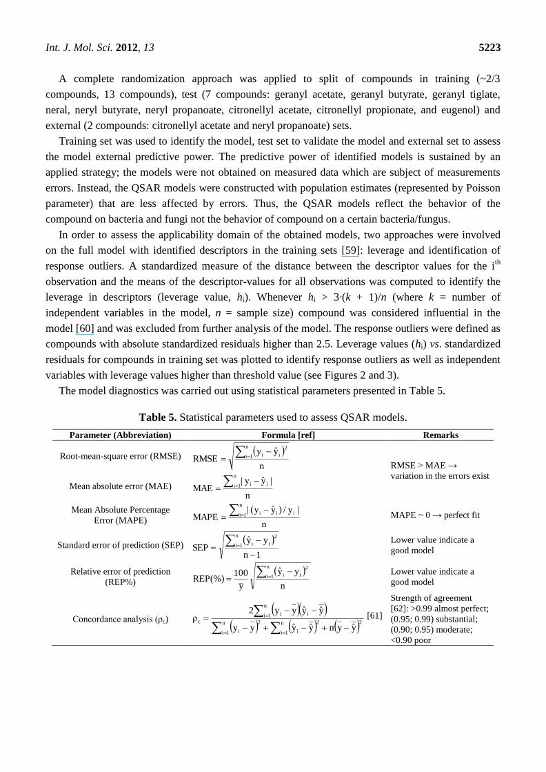
The model diagnostics was carried out using statistical parameters presented in Table 5.

Table 5. Statistical parameters used to assess QSAR models.

Parameter (Abbreviation) Formula [ref] Remarks

Root-mean-square error (RMSE)

n

yyRMSE

n

1i

2

ii

RMSE > MAE →

variation in the errors exist Mean absolute error (MAE)

n

|yy|MAE

n

1i ii

Mean Absolute Percentage

Error (MAPE) n

|y/)yy(|MAPE

n

1i iii

MAPE ~ 0 → perfect fit

Standard error of prediction (SEP)

1n

yySEP

n

1i

2

ii

Lower value indicate a

good model

Relative error of prediction

(REP%)

n

yy

y

100(%)REP

n

1i

2

ii

Lower value indicate a

good model

Concordance analysis (ρc)

n

1i

22

i

n

1i

2

i

n

1i ii

c

yynyyyy

yyyy2ρ [61]

Strength of agreement

[62]: >0.99 almost perfect;

(0.95; 0.99) substantial;

(0.90; 0.95) moderate;

<0.90 poor

Int. J. Mol. Sci. 2012, 13 5224

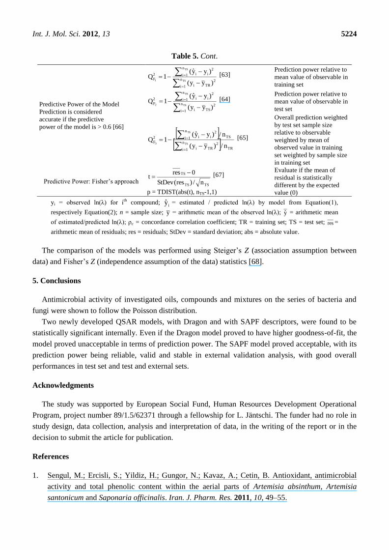
Table 5. Cont.

Predictive Power of the Model

Prediction is considered

accurate if the predictive

power of the model is > 0.6 [66]

TS

TS

1 n

1i

2

TRi

n

1i

2

ii2

F

)yy(

)yy(1Q [63]

Prediction power relative to

mean value of observable in

training set

TS

TS

2 n

1i

2

TSi

n

1i

2

ii2

F

)yy(

)yy(1Q [64]

Prediction power relative to

mean value of observable in

test set

TR

n

1i

2

TRi

TS

n

1i

2

ii2

F

n/)yy(

n/)yy(1Q

TS

TS

3

[65]

Overall prediction weighted

by test set sample size

relative to observable

weighted by mean of

observed value in training

set weighted by sample size

in training set

Predictive Power: Fisher’s approach TSTS

TS

n/)res(StDev

0rest

[67]

p = TDIST(abs(t), nTS-1,1)

Evaluate if the mean of

residual is statistically

different by the expected

value (0)

yi = observed ln(λ) for ith

compound; iy = estimated / predicted ln(λ) by model from Equation(1),

respectively Equation(2); n = sample size; y = arithmetic mean of the observed ln(λ); y = arithmetic mean

of estimated/predicted ln(λ); ρc = concordance correlation coefficient; TR = training set; TS = test set; res =

arithmetic mean of residuals; res = residuals; StDev = standard deviation; abs = absolute value.

The comparison of the models was performed using Steiger’s Z (association assumption between

data) and Fisher’s Z (independence assumption of the data) statistics [68].

5. Conclusions

Antimicrobial activity of investigated oils, compounds and mixtures on the series of bacteria and

fungi were shown to follow the Poisson distribution.

Two newly developed QSAR models, with Dragon and with SAPF descriptors, were found to be

statistically significant internally. Even if the Dragon model proved to have higher goodness-of-fit, the

model proved unacceptable in terms of prediction power. The SAPF model proved acceptable, with its

prediction power being reliable, valid and stable in external validation analysis, with good overall

performances in test set and test and external sets.

Acknowledgments

The study was supported by European Social Fund, Human Resources Development Operational

Program, project number 89/1.5/62371 through a fellowship for L. Jäntschi. The funder had no role in

study design, data collection, analysis and interpretation of data, in the writing of the report or in the

decision to submit the article for publication.

References

1. Sengul, M.; Ercisli, S.; Yildiz, H.; Gungor, N.; Kavaz, A.; Cetin, B. Antioxidant, antimicrobial

activity and total phenolic content within the aerial parts of Artemisia absinthum, Artemisia

santonicum and Saponaria officinalis. Iran. J. Pharm. Res. 2011, 10, 49–55.

Int. J. Mol. Sci. 2012, 13 5225

2. Martini, M.G.; Bizzo, H.R.; Moreira, D.D.; Neufeld, P.M.; Miranda, S.N.; Alviano, C.S.;

Alviano, D.S.; Leitao, S.G. Chemical composition and antimicrobial activities of the essential oils

from Ocimum selloi and hesperozygis myrtoides. Nat. Prod. Commun. 2011, 6, 1027–1030.

3. Serrano, C.; Matos, O.; Teixeira, B.; Ramos, C.; Neng, N.; Nogueira, J.; Nunes, M.L.; Marques, A.

Antioxidant and antimicrobial activity of Satureja montana L. extracts. J. Sci. Food Agric. 2011,

91, 1554–1560.

4. Mothana, R.A.; Alsaid, M.S.; Al-Musayeib, N.M. Phytochemical analysis and in vitro

antimicrobial and free-radical-scavenging activities of the essential oils from Euryops arabicus

and Laggera decurrens. Molecules 2011, 16, 5149–5158.

5. Quintans, L.; da Rocha, R.F.; Caregnato, F.F.; Moreira, J.C.F.; da Silva, F.A.; Araujo, A.A.D.;

dos Santos, J.P.A.; Melo, M.S.; de Sousa, D.P.; Bonjardim, L.R.; Gelain, D.P. Antinociceptive

action and redox properties of citronellal, an essential oil present in lemongrass. J. Med. Food

2011, 14, 630–639.

6. Ito, K.; Ito, M. Sedative effects of vapor inhalation of the essential oil of Microtoena patchoulii

and its related compounds. J. Nat. Med. 2011, 65, 336–343.

7. Garozzo, A.; Timpanaro, R.; Stivala, A.; Bisignano, G.; Castro, A. Activity of Melaleuca

alternifolia (tea tree) oil on influenza virus A/PR/8: Study on the mechanism of action. Antivir.

Res. 2011, 89, 83–88.

8. Pauli, A. Anticandidal low molecular compounds from higher plants with special reference to

compounds from essential oils. Med. Res. Rev. 2011, 26, 223–268.

9. Jaffri, J.M.; Mohamed, S.; Ahmad, I.N.; Mustapha, N.M.; Manap, Y.A.; Rohimi, N. Effects of

catechin-rich oil palm leaf extract on normal and hypertensive rats’ kidney and liver. Food Chem.

2011, 128, 433–441.

10. Yu, F.; Gao, J.; Zeng, Y.; Liu, C.X. Effects of adlay seed oil on blood lipids and antioxidant

capacity in hyperlipidemic rats. J. Sci. Food Agric. 2011, 91, 1843–1848.

11. Zhang, Y.B.; Guo, J.; Dong, H.Y.; Zhao, X.M.; Zhou, L.; Li, X.Y.; Liu, J.C.; Niu, Y.C.

Hydroxysafflor yellow a protects against chronic carbon tetrachloride-induced liver fibrosis.

Eur. J. Pharmacol. 2011, 660, 438–444.

12. Yordi, E.G.; Molina Pérez, E.; Joao Matos, M.; Uriarte Villares, E. Structural alerts for predicting

clastogenic activity of pro-oxidant flavonoid compounds: Quantitative structure-activity

relationship study. J. Biomol. Screen. 2012, 17, 216–224.

13. Rishton, G.M. Natural products as a robust source of new drugs and drug leads: Past successes

and present day issues. Am. J. Cardiol. 2008, 101, 43D–49D.

14. Dunn, W.J., III. Quantitative structure-activity relationships (QSAR). Chemom. Intell. Lab. 1989,

6, 181–190.

15. Khan, F.; Yadav, D.K.; Maurya, A.; Srivastava, S.K. Modern methods & web resources in drug

design & discovery. Lett. Drug Des. Discov. 2011, 8, 469–490.

16. Vedani, A.; Dobler, M.; Spreafico, M.; Peristera, O.; Smiesko, M. VirtualToxLab—in silico

prediction of the toxic potential of drugs and environmental chemicals: Evaluation status and

internet access protocol. Altex 2007, 24, 153–161.

17. Castro, E.A. QSPR-QSAR Studies on Desired Properties for Drug Design; Research Signpost:

Kerala, India, 2010.

Int. J. Mol. Sci. 2012, 13 5226

18. Gasteiger, J.; Engel, T. Chemoinformatics: A Textbook, 1st ed.; Wiley-VCH: Weinheim, Germany,

2003.

19. Alvarez, J.; Shoichet, B. Virtual Screening in Drug Discovery, 1st ed.; CRC Press: Boca Raton,

FL, USA, 2005.

20. Schuster, D.; Wolber, G. Identification of bioactive natural products by pharmacophore-based

virtual screening. Curr. Pharm. Des. 2010, 16, 1666–1681.

21. Bartalis, J.; Halaweish, F.T. In vitro and QSAR studies of cucurbitacins on HepG2 and HSC-T6

liver cell lines. Bioorg. Med. Chem. 2011, 19, 2757–2766.

22. Bolboacă, S.D.; Pică, E.M.; Cimpoiu, C.V.; Jäntschi, L. Statistical assessment of solvent mixture

models used for separation of biological active compounds. Molecules 2008, 13, 1617–1639.

23. González-Díaz, H.; Torres-Gomez, L.A.; Guevara, Y.; Almeida, M.S.; Molina, R.; Castanedo, N.;

Castañedo, N.; Santana, L.; Uriarte, E. Markovian chemicals ―in silico‖ design

(MARCH-INSIDE), a promising approach for computer-aided molecular design III: 2.5D indices

for the discovery of antibacterials. J. Mol. Model. 2005, 11, 116–123.

24. Gonzalez-Diaz, H.; Prado-Prado, F.; Ubeira, F.M. Predicting antimicrobial drugs and targets with

the MARCH-INSIDE approach. Curr. Top. Med. Chem. 2008, 8, 1676–90.

25. Molina, E.; Díaz, H.G.; González, M.P.; Rodríguez, E.; Uriarte, E. Designing antibacterial

compounds through a topological substructural approach. J. Chem. Inf. Comput. Sci. 2004, 44,

515–521.

26. González-Díaz, H.; Romaris, F.; Duardo-Sanchez, A.; Pérez-Montoto, L.G.; Prado-Prado, F.;

Patlewicz, G.; Ubeira, F.M. Predicting drugs and proteins in parasite infections with topological

indices of complex networks: Theoretical backgrounds, applications and legal issues.

Curr. Pharm. Des. 2010, 16, 2737–2764.

27. Prado-Prado, F.J.; Gonzalez-Diaz, H.; Santana, L.; Uriarte, E. Unified QSAR approach to

antimicrobials. Part 2: Predicting activity against more than 90 different species in order to halt

antibacterial resistance. Bioorg. Med. Chem. 2007, 15, 897–902.

28. Prado-Prado, F.J.; Uriarte, E.; Borges, F.; González-Díaz, H. Multi-target spectral moments for

QSAR and complex networks study of antibacterial drugs. Eur. J. Med. Chem. 2009, 44, 4516–4521.

29. Gonzalez-Diaz, H.; Prado-Prado, F.J. Unified QSAR and network-based computational chemistry

approach to antimicrobials, part 1: Multispecies activity models for antifungals. J. Comput. Chem.

2008, 29, 656–667.

30. Prado-Prado, F.J.; Ubeira, F.M.; Borges, F.; Gonzalez-Diaz, H. Unified QSAR & network-based

computational chemistry approach to antimicrobials. II. Multiple distance and triadic census

analysis of antiparasitic drugs complex networks. J. Comput. Chem. 2010, 31, 164–173.

31. Prado-Prado, F.J.; Martinez de la Vega, O.; Uriarte, E.; Ubeira, F.M.; Chou, K.C.; Gonzalez-Diaz, H.

Unified QSAR approach to antimicrobials. 4. Multi-target QSAR modeling and comparative

multi-distance study of the giant components of antiviral drug-drug complex networks.

Bioorg. Med. Chem. 2009, 17, 569–575.

32. Gonzalez-Diaz, H.; Prado-Prado, F.; Sobarzo-Sanchez, E.; Haddad, M.; Maurel Chevalley, S.;

Valentin, A.; Quetin-Leclercq, J.; Dea-Ayuela, M.A.; Teresa Gomez-Muños, M.; Munteanu, C.R.

NL MIND-BEST: A web server for ligands and proteins discovery-theoretic-experimental study

Int. J. Mol. Sci. 2012, 13 5227

of proteins of Giardia lamblia and new compounds active against Plasmodium falciparum.

J. Theor. Biol. 2011, 276, 229–249

33. Jirovetz, L.; Eller, G.; Buchbauer, G.; Schmidt, E.; Denkova, Z.; Stoyanova, A.S.; Nikolova, R.;

Geissler, M. Chemical composition, antimicrobial activities and odor descriptions of some

essential oils with characteristic. Recent Res. Dev. Agron. Hortic. 2006, 2, 1–12.

34. Fisher, R.A. On an absolute criterion for fitting frequency curves. Messenger Math. 1912, 41,

155–160.

35. Sacks, J.; Ylvisaker, D. Designs for regression problems with correlated errors III. Ann. Math.

Stat. 1970, 41, 2057–2074.

36. Jarque, C.M.; Bera, A.K. A test for normality of observations and regression residuals. Int. Stat.

Rev. 1987, 55, 163–172.

37. LeRoy, J.S. Negative Binomial and Poisson Distributions Compared. In Proceedings of the

Casualty Actuarial Society; Casualty Actuarial Society: Arlington, VA, USA, 1960; Volume

XLVII, Numbers 87 & 88, pp. 20–24. Available online: http://www.casact.org/pubs/proceed/

proceed60/60020.pdf (accessed on 6 August 2011).

38. Furman, E. On the convolution of the negative binomial random variables. Stat. Probab. Lett.

2007, 77, 169–172.

39. Jones, A. Health Econometrics. In Handbook of Health Economics; Culyer, A., Newhouse, J., Eds.;

Elsevier: Amsterdam, The Netherland, 2000.

40. Cameron, A.C.; Trivedi, P.K. Regression Analysis of Count Data; Cambridge University Press:

London, UK, 1998.

41. Fisher R.A. A theoretical distribution for the apparent abundance of different species. J. Anim.

Ecol. 1943, 12, 54–58.

42. Shaked, M. A family of concepts of dependence for bivariate distributions. J. Am. Stat. Assoc.

1977, 72, 642–650.

43. Marshall, A.W.; Olkin, I. Multivariate distributions generated from mixtures of convolution and

product families, lecture notes-monograph series. Top. Stat. Depend. 1990, 16, 371–393.

44. Jäntschi, L.; Bolboacă, S.D.; Bălan, M.C.; Sestraş, R.E. Distribution fitting 13. Analysis of

independent, multiplicative effect of factors. Application to effect of essential oils extracts from

plant species on bacterial species. Application to factors of antibacterial activity of plant species.

Bull. Univ. Agric. Sci. Vet. Med. Cluj-Napoca. Anim. Sci. Biotechnol. 2011, 68, 323–331.

45. Kundu, D.; Manglick, A. Discriminating between the log-normal and gamma distributions.

Available online: http://home.iitk.ac.in/~kundu/paper93.pdf (accessed on 1 August 2011).

46. Bolboacă, S.D.; Jäntschi, L. Modelling the property of compounds from structure: Statistical

methods for models validation. Environ. Chem. Lett. 2008, 6, 175–181.

47. Kolmogorov, A. Confidence limits for an unknown distribution function. Ann. Math. Stat. 1941,

12, 461–463.

48. Anderson, T.W.; Darling, D.A. Asymptotic theory of certain ―goodness-of-fit‖ criteria based on

stochastic processes. Ann. Math. Stat. 1952, 23, 193–212.

49. Fisher, R.A. Combining independent tests of significance. Am. Stat. 1948, 2, 30.

Int. J. Mol. Sci. 2012, 13 5228

50. Hobza, P.; Kabeláč, M.; Šponer, J.; Mejzlík, P.; Vondrášek, J. Performance of empirical potentials

(AMBER, CFF95, CVFF, CHARMM, OPLS, POLTEV), semiempirical quantum chemical

methods (AM1, MNDO/M, PM3), and Ab initio Hartree-Fock method for interaction of DNA

bases: Comparison with nonempirical beyond Hartree-Fock results. J. Comput. Chem. 1997, 18,

1136–1150.

51. HyperChem, version 8.0; Hypercube Inc.: Gainesville, FL, USA, 2007.

52. Jäntschi, L. Computer assisted geometry optimization for in silico modeling. Appl. Med. Inform.

2011, 29, 11–18.

53. Jäntschi, L. Genetic Algorithms and Their Applications (in Romanian). Ph.D. Dissertation,

University of Agricultural Sciences and Veterinary Medicine, Cluj-Napoca, Romania, 2010.

54. Jäntschi, L.; Bolboacă, S.D.; Sestraş, R.E. Quantum Mechanics Study on a Series of Steroids

Relating Separation with Structure; In Proceedings of 17th International Symposium on

Separation Sciences: Book of Abstracts, Cluj-Napoca, Romania, September 5–9, 2011;

Casa Cărţii de Ştiinţă: Cluj-Napoca, Romania, 2011; p. 59.

55. DRAGON, version 5.5; Talete srl: Milano, Italy, 2007.

56. Pauling, L. The nature of the chemical bond. IV. The energy of single bonds and the relative

electronegativity of atoms. J. Am. Chem. Soc. 1932, 54, 3570–3582.

57. Jäntschi, L.; Bolboacă, S.D. Distribution Fitting 2. Pearson-Fisher, Kolmogorov-Smirnov,

Anderson-Darling, Wilks-Shapiro, Kramer-von-Misses and Jarque-Bera statistics. Bull. Univ.

Agric. Sci. Vet. Med. Cluj-Napoca. Hortic. 2009, 66, 691–697.

58. Grubbs, F. Procedures for detecting outlying observations in samples. Technometrics 1969, 11, 1–21.

59. Chatterjee, S.; Hadi, A.S. Influential observations, high leverage points, and outliers in linear

regression (with discussion). Stat. Sci. 1986, 1, 379–416.

60. Eriksson, L.; Jaworska, J.; Worth, A.P.; Cronin, M.T.D.; McDowell, R.M.; Gramatica, P.

Methods for reliability and uncertainty assessment and for applicability evaluations of

classification and regression-based QSARs. Environ. Health Perspect. 2003, 111, 1361–1375.

61. Chirico, N.; Gramatica, P. Real external predictivity of QSAR models: How to evaluate it?

Comparison of different validation criteria and proposal of using the concordance correlation

coefficient. J. Chem. Inf. Model. 2011, 51, 2320–2335.

62. McBride, G.B. A Proposal for Strength-of-Agreement Criteria for Lin’S Concordance

Correlation Coefficient; NIWA Client Report: HAM2005-062; National Institute of Water &

Atmospheric Research: Hamilton, New Zeeland, May 2005. Available online:

http://www.medcalc.org/download/pdf/McBride2005.pdf (accessed on 14 March 2012).

63. Shi, L.M.; Fang, H.; Tong, W.; Wu, J.; Perkins, R.; Blair, R.M.; Branham, W.S.; Dial, S.L.;

Moland, C.L.; Sheehan, D.M. QSAR models using a large diverse set of estrogens. J. Chem. Inf.

Comput. Sci. 2001, 41, 186–195.

64. Schüürmann, G.; Ebert, R.U.; Chen, J.; Wang, B.; Kühne, R. External validation and prediction

employing the predictive squared correlation coefficient test set activity mean vs. training set

activity mean. J. Chem. Inf. Model. 2008, 48, 2140–2145.

65. Consonni, V.; Ballabio, D.; Todeschini, R. Comments on the definition of the Q2 parameter for

QSAR validation. J. Chem. Inf. Model. 2009, 49, 1669–1678.

66. Golbraikh, A.; Tropsha, A. Beware of q2! J. Mol. Gr. Mod. 2002, 20, 269–276.

Int. J. Mol. Sci. 2012, 13 5229

67. Fisher, R.A. The goodness of fit of regression formulae, and the distribution of regression

coefficients. J. Royal Stat. Soc. 1922, 85, 597–612.

68. Steiger, J.H. Tests for comparing elements of a correlation matrix. Psychol. Bull. 1980, 87,

245–251.

© 2012 by the authors; licensee MDPI, Basel, Switzerland. This article is an open access article

distributed under the terms and conditions of the Creative Commons Attribution license

(http://creativecommons.org/licenses/by/3.0/).