Point Operations Histogram Processing

BBM 413 ��Fundamentals of ��Image Processing

Erkut Erdem��Dept. of Computer Engineering��

Hacettepe University��

Point Operations Histogram Processing

Today’s topics

•  Point operations

•  Histogram processing

Today’s topics



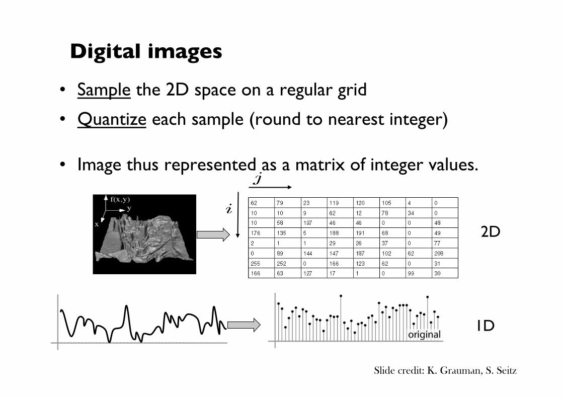
Digital images

•  Sample the 2D space on a regular grid

•  Quantize each sample (round to nearest integer)

•  Image thus represented as a matrix of integer values.

Slide credit: K. Grauman, S. Seitz

2D

1D

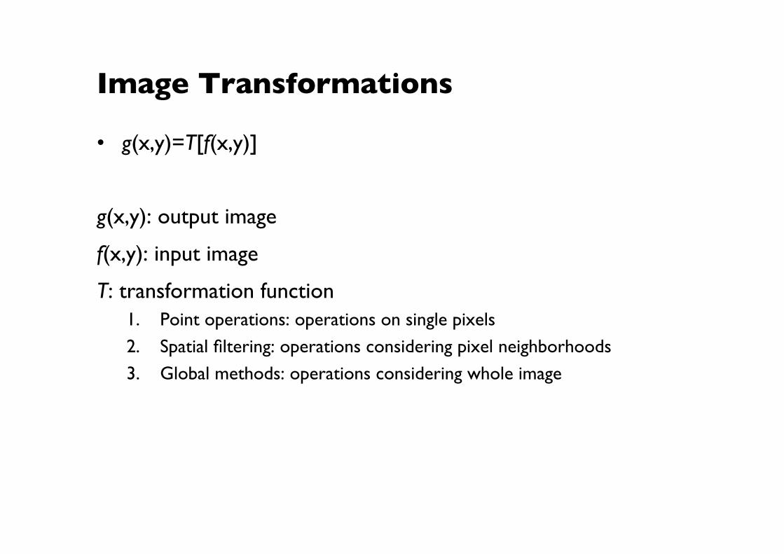
Image Transformations

•  g(x,y)=T[f(x,y)]

g(x,y): output image

f(x,y): input image

T: transformation function 1.  Point operations: operations on single pixels

2.  Spatial filtering: operations considering pixel neighborhoods

3.  Global methods: operations considering whole image

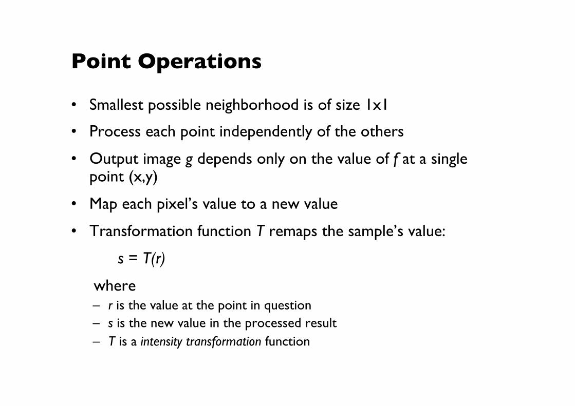
Point Operations

•  Smallest possible neighborhood is of size 1x1

•  Process each point independently of the others

•  Output image g depends only on the value of f at a single point (x,y)

•  Map each pixel’s value to a new value

•  Transformation function T remaps the sample’s value:

s = T(r)

where –  r is the value at the point in question –  s is the new value in the processed result –  T is a intensity transformation function

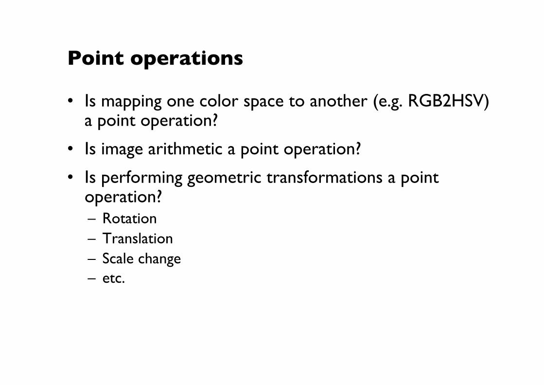
Point operations

•  Is mapping one color space to another (e.g. RGB2HSV) a point operation?

•  Is image arithmetic a point operation?

•  Is performing geometric transformations a point operation? –  Rotation –  Translation –  Scale change –  etc.

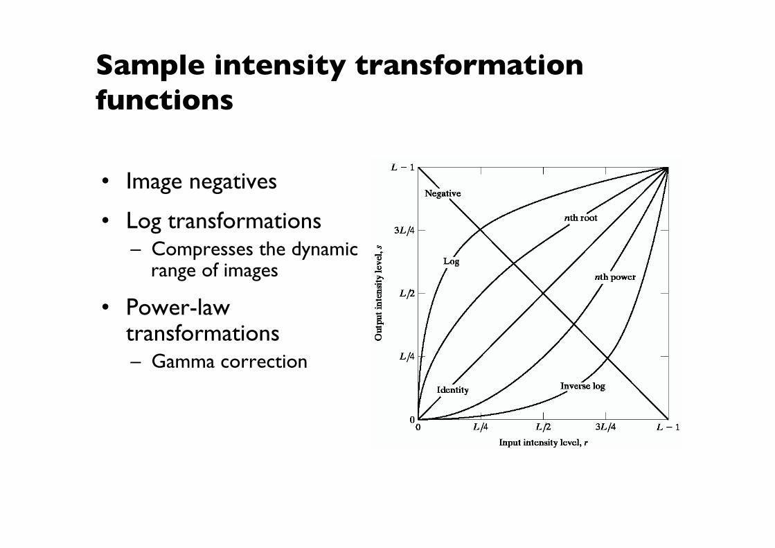
Sample intensity transformation functions

•  Image negatives

•  Log transformations –  Compresses the dynamic

range of images

•  Power-law transformations –  Gamma correction

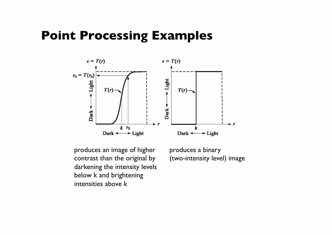
Point Processing Examples

produces an image of higher��contrast than the original by��darkening the intensity levels��below k and brightening ��intensities above k

produces a binary ��(two-intensity level) image

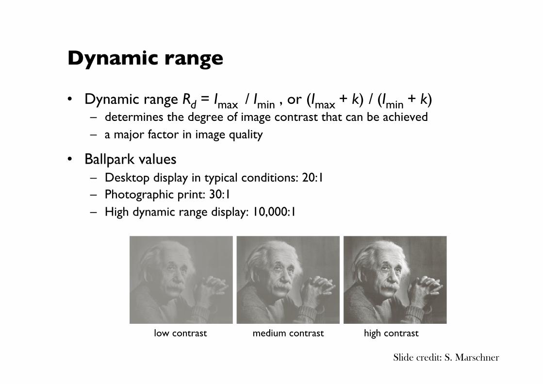
Dynamic range

•  Dynamic range Rd = Imax / Imin , or (Imax + k) / (Imin + k) –  determines the degree of image contrast that can be achieved –  a major factor in image quality

•  Ballpark values –  Desktop display in typical conditions: 20:1 –  Photographic print: 30:1 –  High dynamic range display: 10,000:1

low contrast medium contrast high contrast

Slide credit: S. Marschner

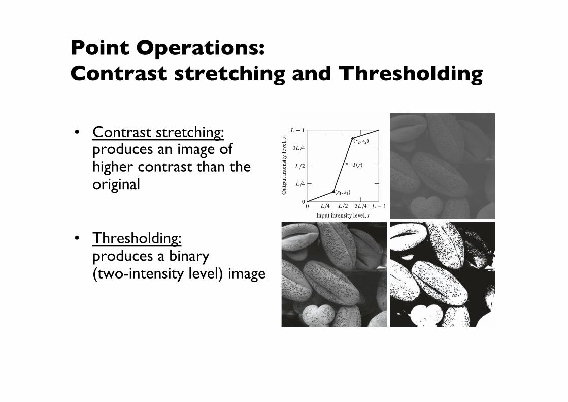
Point Operations: ��Contrast stretching and Thresholding

•  Contrast stretching: produces an image of higher contrast than the original

•  Thresholding: ��produces a binary ��(two-intensity level) image

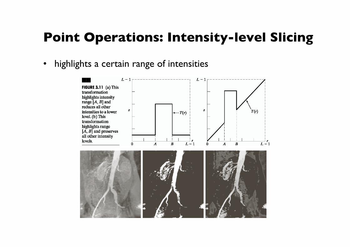
Point Operations: Intensity-level Slicing

•  highlights a certain range of intensities

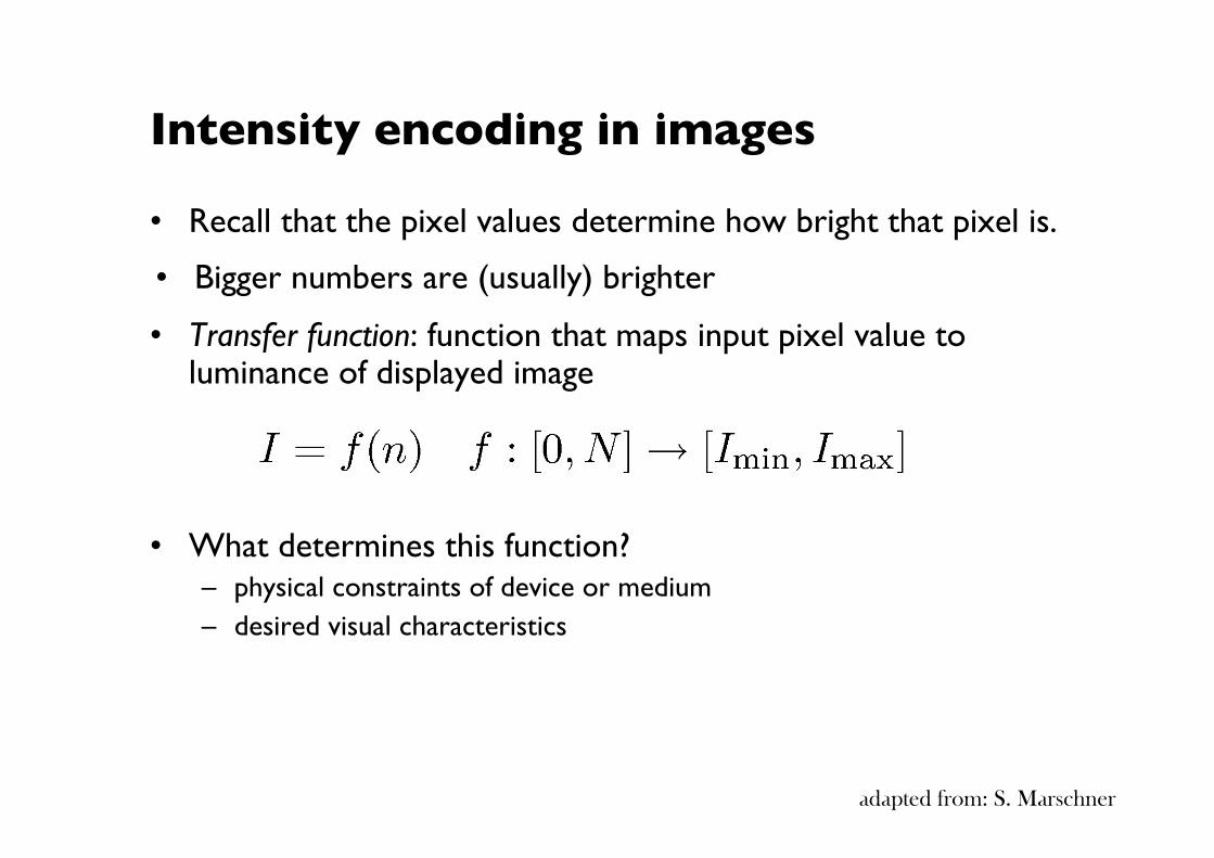
Intensity encoding in images

•  Recall that the pixel values determine how bright that pixel is.

•  Bigger numbers are (usually) brighter

•  Transfer function: function that maps input pixel value to luminance of displayed image

•  What determines this function? –  physical constraints of device or medium –  desired visual characteristics

adapted from: S. Marschner

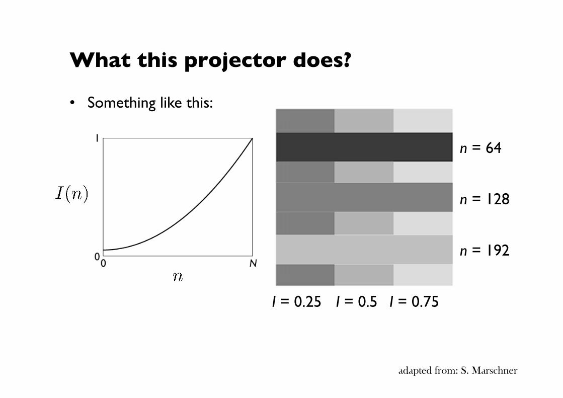
What this projector does?

n = 64

n = 128

n = 192

I = 0.25 I = 0.5 I = 0.75

•  Something like this:

adapted from: S. Marschner

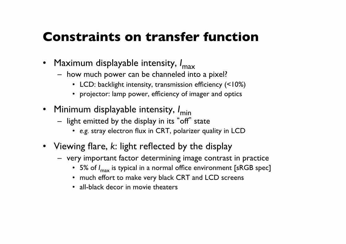
Constraints on transfer function

•  Maximum displayable intensity, Imax –  how much power can be channeled into a pixel?

•  LCD: backlight intensity, transmission efficiency (<10%) •  projector: lamp power, efficiency of imager and optics

•  Minimum displayable intensity, Imin –  light emitted by the display in its “off” state

•  e.g. stray electron flux in CRT, polarizer quality in LCD

•  Viewing flare, k: light reflected by the display –  very important factor determining image contrast in practice

•  5% of Imax is typical in a normal office environment [sRGB spec] •  much effort to make very black CRT and LCD screens •  all-black decor in movie theaters

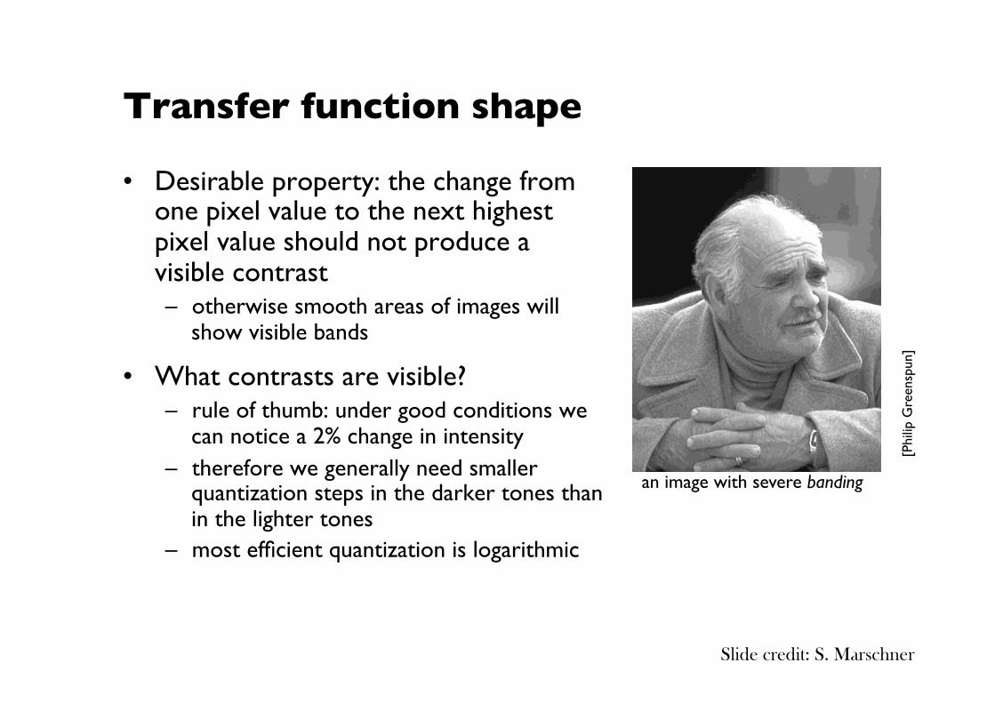
Transfer function shape

•  Desirable property: the change from one pixel value to the next highest pixel value should not produce a visible contrast –  otherwise smooth areas of images will

show visible bands

•  What contrasts are visible? –  rule of thumb: under good conditions we

can notice a 2% change in intensity –  therefore we generally need smaller

quantization steps in the darker tones than in the lighter tones

–  most efficient quantization is logarithmic

an image with severe banding

[Phi

lip G

reen

spun

]


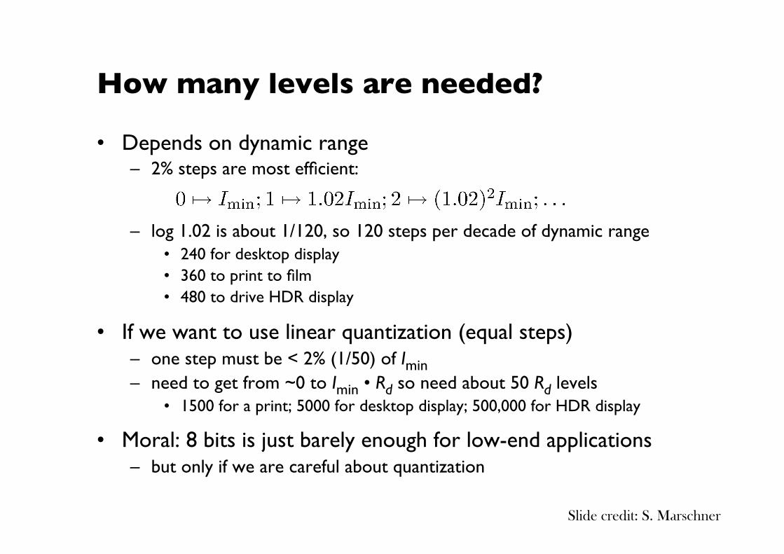
How many levels are needed?

•  Depends on dynamic range –  2% steps are most efficient:

–  log 1.02 is about 1/120, so 120 steps per decade of dynamic range •  240 for desktop display •  360 to print to film •  480 to drive HDR display

•  If we want to use linear quantization (equal steps) –  one step must be < 2% (1/50) of Imin –  need to get from ~0 to Imin • Rd so need about 50 Rd levels

•  1500 for a print; 5000 for desktop display; 500,000 for HDR display

•  Moral: 8 bits is just barely enough for low-end applications –  but only if we are careful about quantization


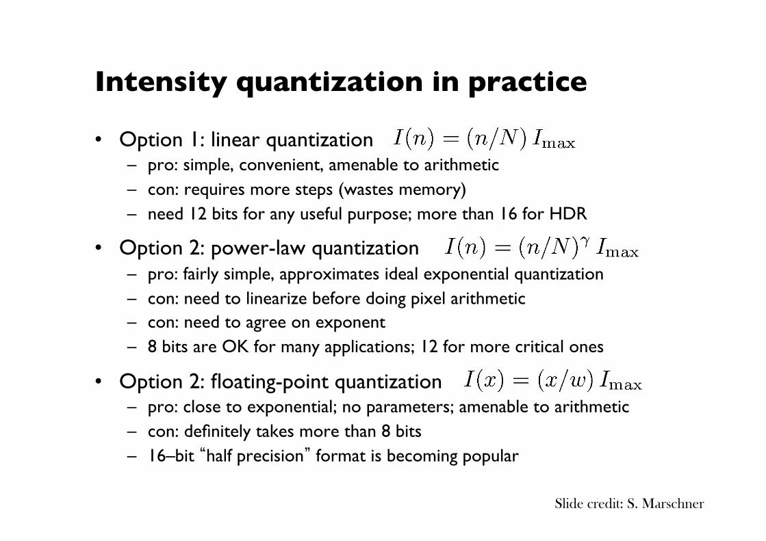
Intensity quantization in practice

•  Option 1: linear quantization –  pro: simple, convenient, amenable to arithmetic –  con: requires more steps (wastes memory) –  need 12 bits for any useful purpose; more than 16 for HDR

•  Option 2: power-law quantization –  pro: fairly simple, approximates ideal exponential quantization –  con: need to linearize before doing pixel arithmetic –  con: need to agree on exponent –  8 bits are OK for many applications; 12 for more critical ones

•  Option 2: floating-point quantization –  pro: close to exponential; no parameters; amenable to arithmetic –  con: definitely takes more than 8 bits –  16–bit “half precision” format is becoming popular


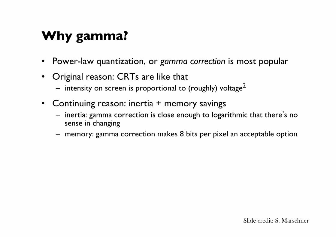
Why gamma?

•  Power-law quantization, or gamma correction is most popular

•  Original reason: CRTs are like that –  intensity on screen is proportional to (roughly) voltage2

•  Continuing reason: inertia + memory savings –  inertia: gamma correction is close enough to logarithmic that there’s no

sense in changing –  memory: gamma correction makes 8 bits per pixel an acceptable option


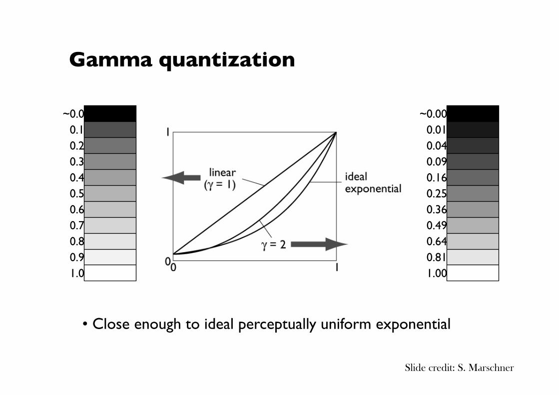
Gamma quantization

~0.00 0.01 0.04 0.09 0.16 0.25 0.36 0.49 0.64 0.81 1.00

~0.0 0.1 0.2 0.3 0.4 0.5 0.6 0.7 0.8 0.9 1.0

• Close enough to ideal perceptually uniform exponential


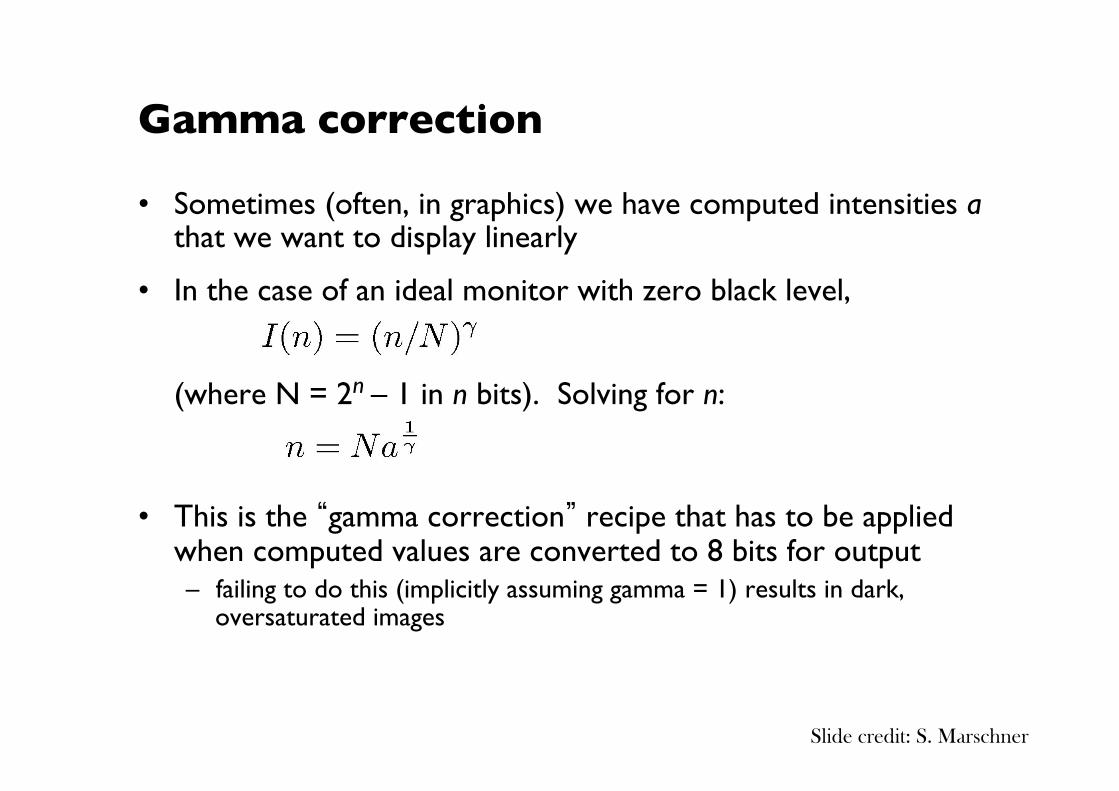
Gamma correction

•  Sometimes (often, in graphics) we have computed intensities a that we want to display linearly

•  In the case of an ideal monitor with zero black level, ��(where N = 2n – 1 in n bits). Solving for n: ��

•  This is the “gamma correction” recipe that has to be applied when computed values are converted to 8 bits for output –  failing to do this (implicitly assuming gamma = 1) results in dark,

oversaturated images


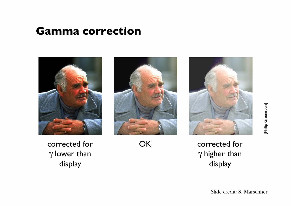
Gamma correction

[Phi

lip G

reen

spun

]

OK corrected for γ lower than

display

corrected for γ higher than

display


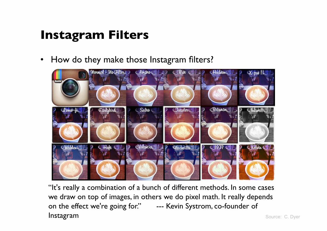
Instagram Filters

•  How do they make those Instagram filters?

“It's really a combination of a bunch of different methods. In some cases we draw on top of images, in others we do pixel math. It really depends on the effect we're going for.” --- Kevin Systrom, co-founder of Instagram��

Source: C. Dyer

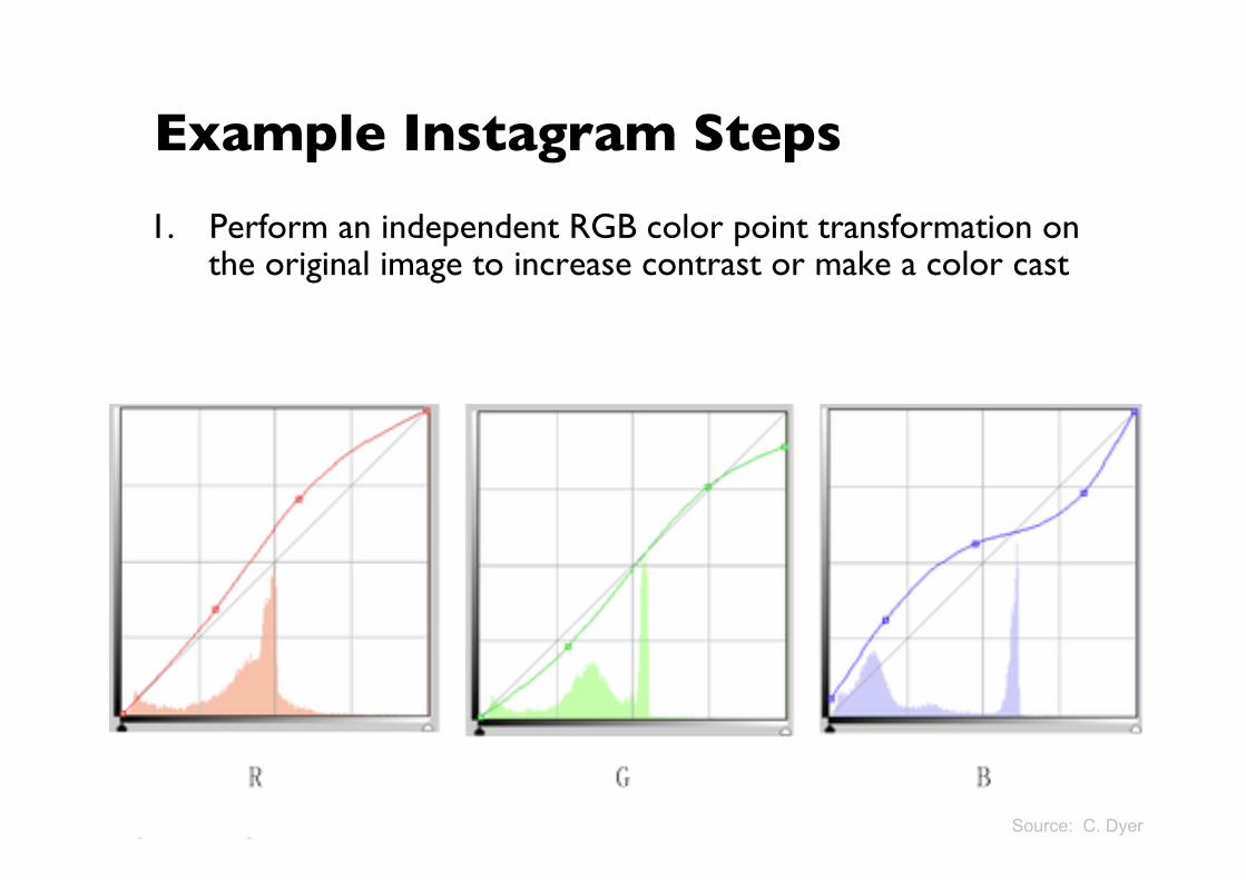
Example Instagram Steps 1.  Perform an independent RGB color point transformation on

the original image to increase contrast or make a color cast

Source: C. Dyer

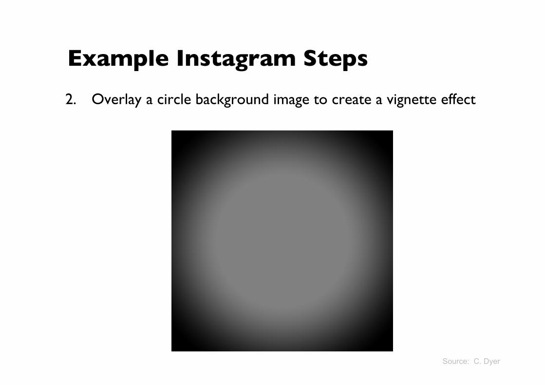
Example Instagram Steps 2.  Overlay a circle background image to create a vignette effect

Source: C. Dyer

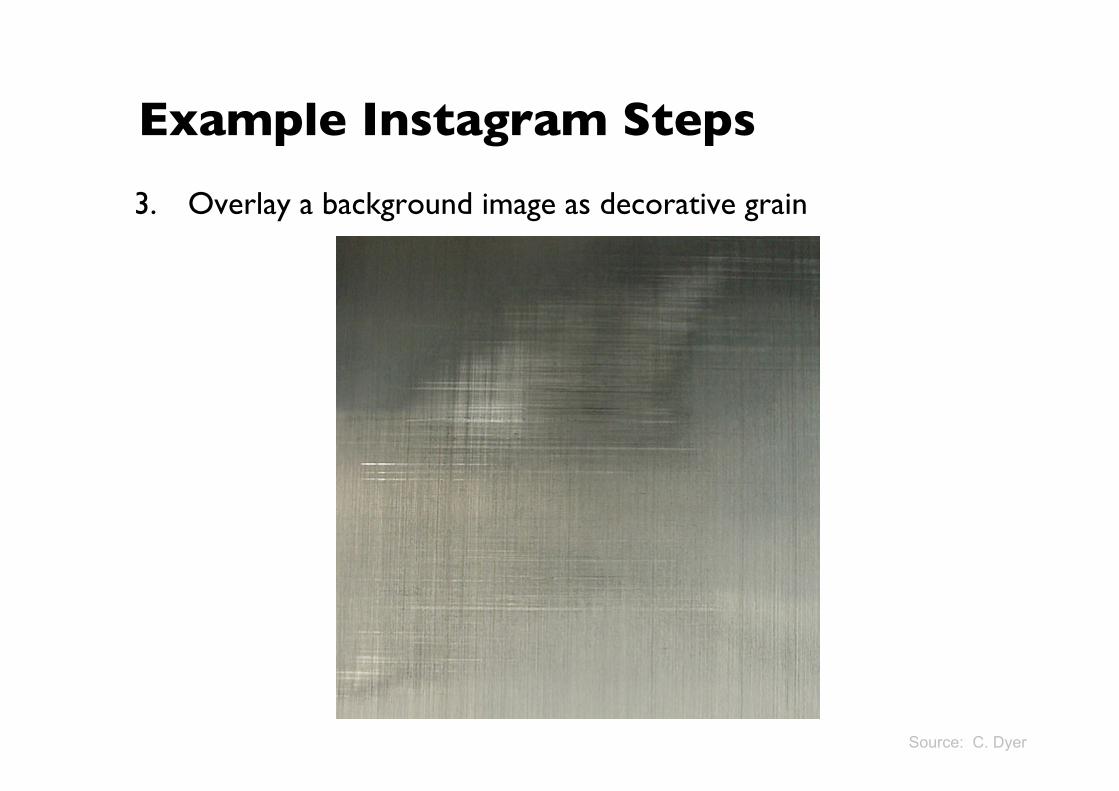
Example Instagram Steps 3.  Overlay a background image as decorative grain

Source: C. Dyer

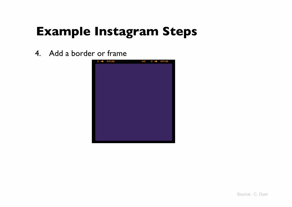
Example Instagram Steps 4.  Add a border or frame

Source: C. Dyer

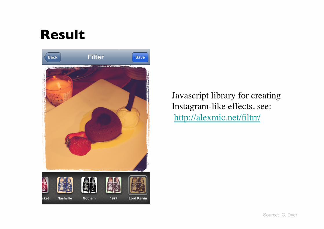
Result

Javascript library for creating Instagram-like effects, see: http://alexmic.net/filtrr/

Source: C. Dyer

Today’s topics



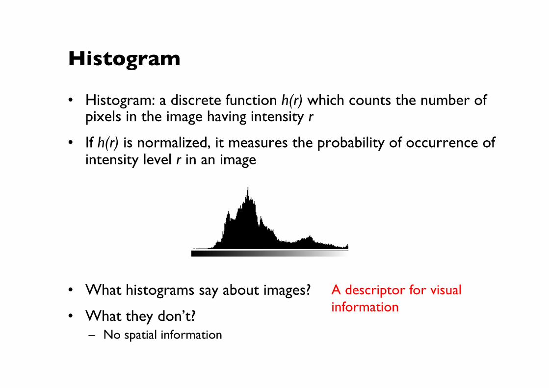
Histogram

•  Histogram: a discrete function h(r) which counts the number of pixels in the image having intensity r

•  If h(r) is normalized, it measures the probability of occurrence of intensity level r in an image

•  What histograms say about images?

•  What they don’t? –  No spatial information

Level Operations (Part 2)

Histograms

Histograms

A histogram H(r) counts how many times each quantized valueoccurs.

Example:

A descriptor for visual ��information

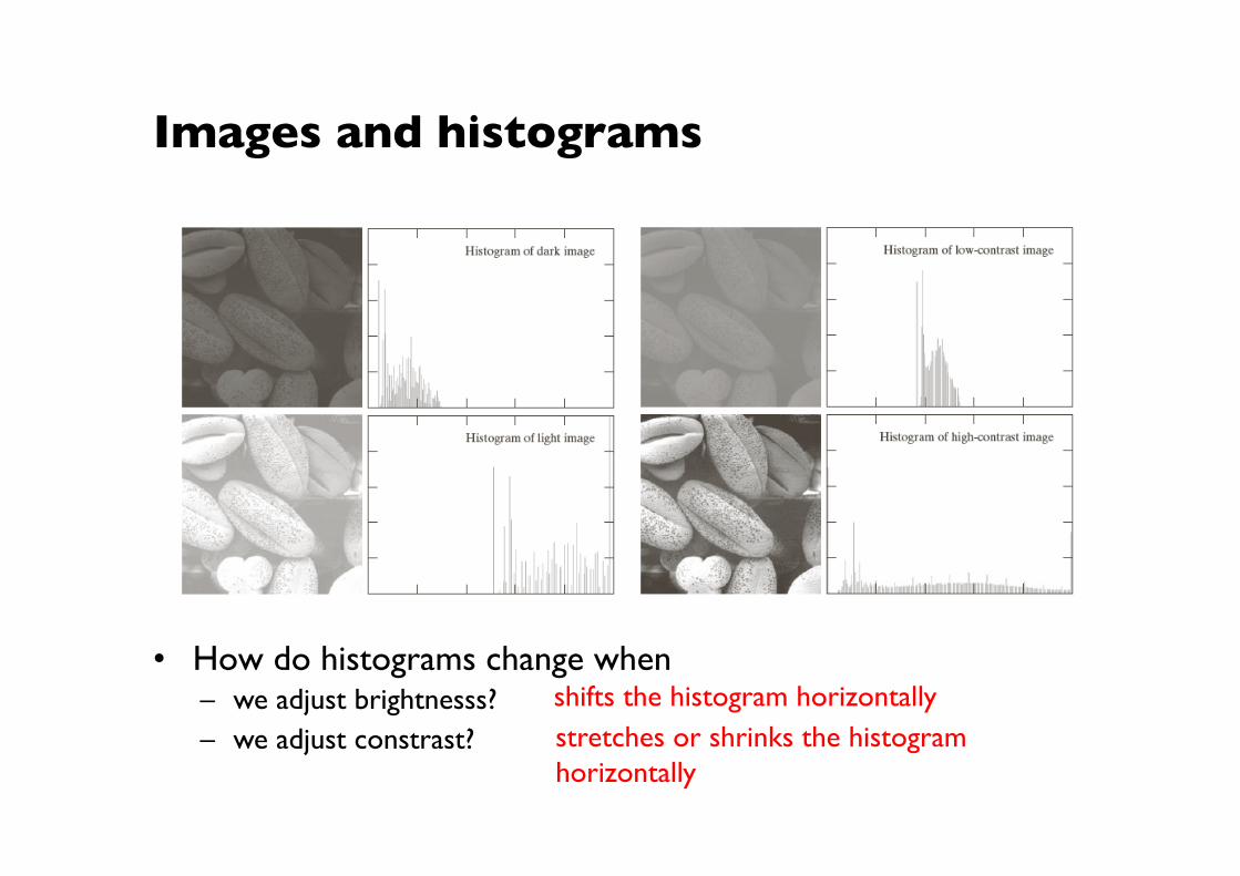
Images and histograms

•  How do histograms change when –  we adjust brightnesss? –  we adjust constrast?

shifts the histogram horizontally stretches or shrinks the histogram horizontally

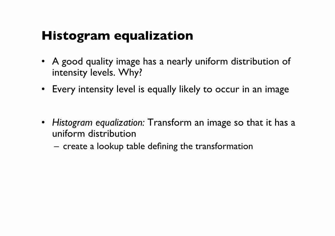
Histogram equalization

•  A good quality image has a nearly uniform distribution of intensity levels. Why?

•  Every intensity level is equally likely to occur in an image

•  Histogram equalization: Transform an image so that it has a uniform distribution –  create a lookup table defining the transformation

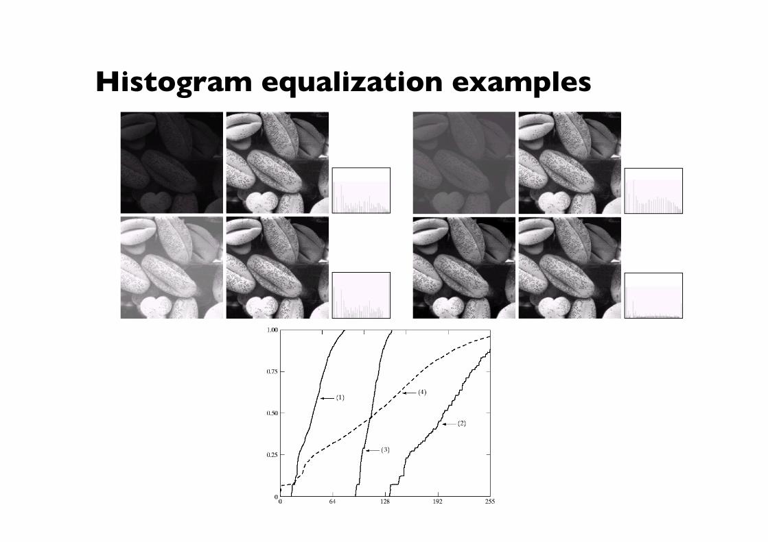
Histogram equalization examples


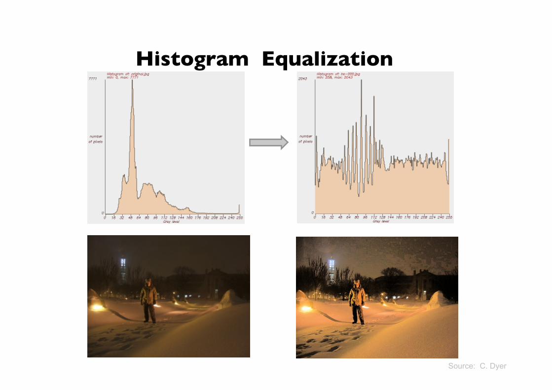
Histogram Equalization

Histogram Equalization: Examples








Source: C. Dyer

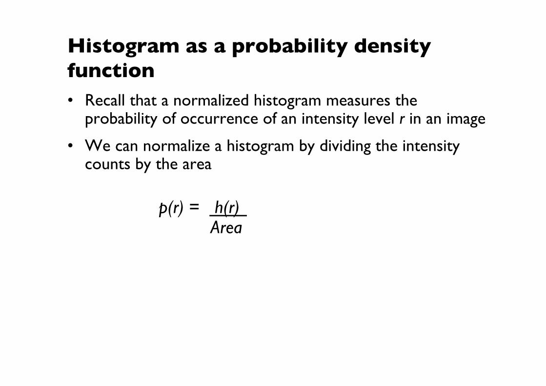
Histogram as a probability density function •  Recall that a normalized histogram measures the

probability of occurrence of an intensity level r in an image

•  We can normalize a histogram by dividing the intensity counts by the area

p(r) = h(r) Area

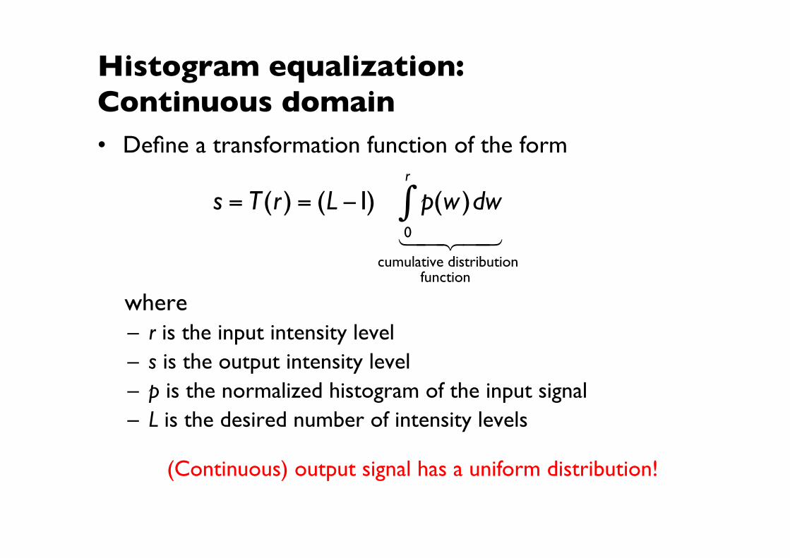
Histogram equalization: ��Continuous domain •  Define a transformation function of the form

where –  r is the input intensity level –  s is the output intensity level –  p is the normalized histogram of the input signal –  L is the desired number of intensity levels

s = T(r) = (L −1) p(w )dw0

r

∫cumulative distribution function

(Continuous) output signal has a uniform distribution!

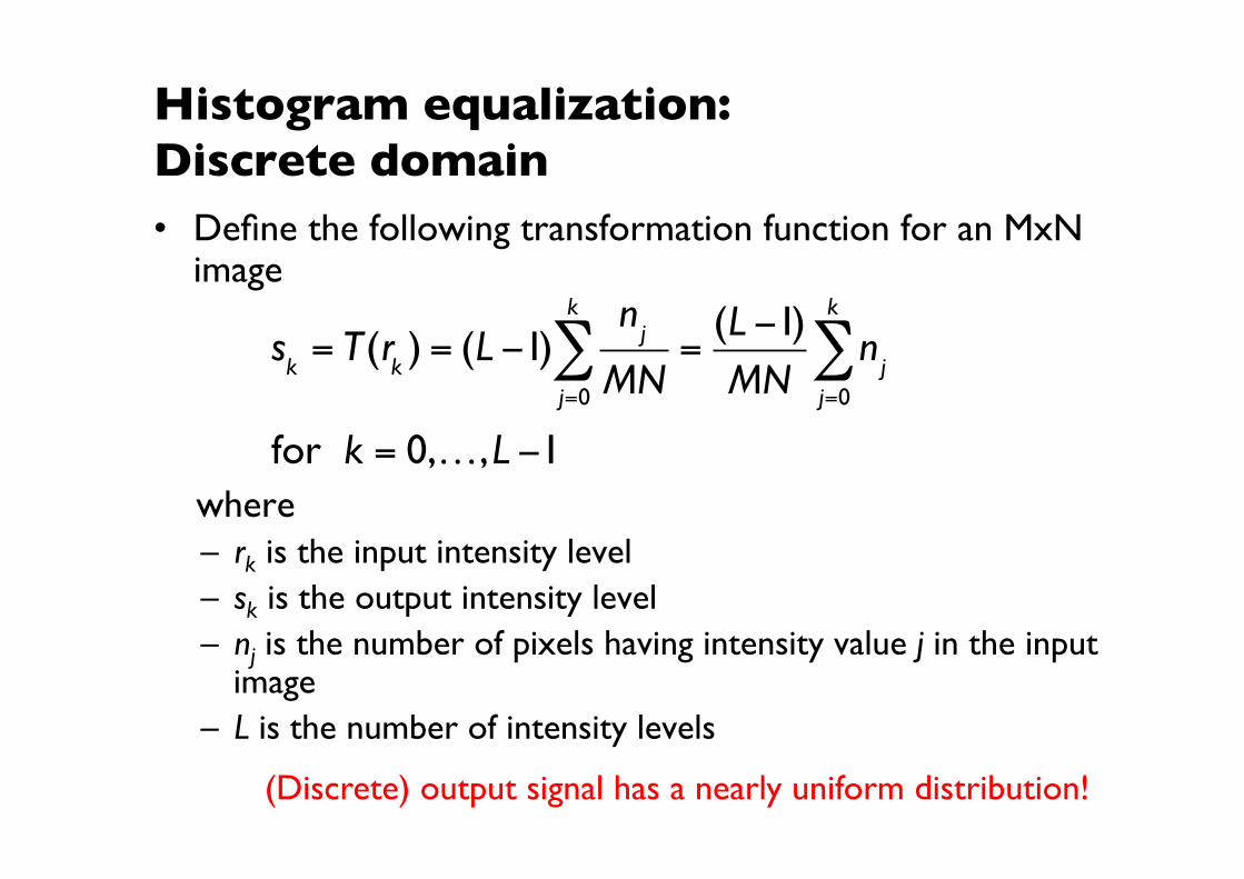
Histogram equalization: ��Discrete domain •  Define the following transformation function for an MxN

image

where –  rk is the input intensity level –  sk is the output intensity level –  nj is the number of pixels having intensity value j in the input

image –  L is the number of intensity levels

sk= T(r

k) = (L −1)

nj

MNj=0

k

∑ =(L −1)MN

nj

j=0

k

∑

for k = 0,…,L −1

(Discrete) output signal has a nearly uniform distribution!

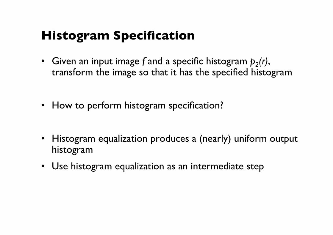
Histogram Specification

•  Given an input image f and a specific histogram p2(r), transform the image so that it has the specified histogram

•  How to perform histogram specification?

•  Histogram equalization produces a (nearly) uniform output histogram

•  Use histogram equalization as an intermediate step

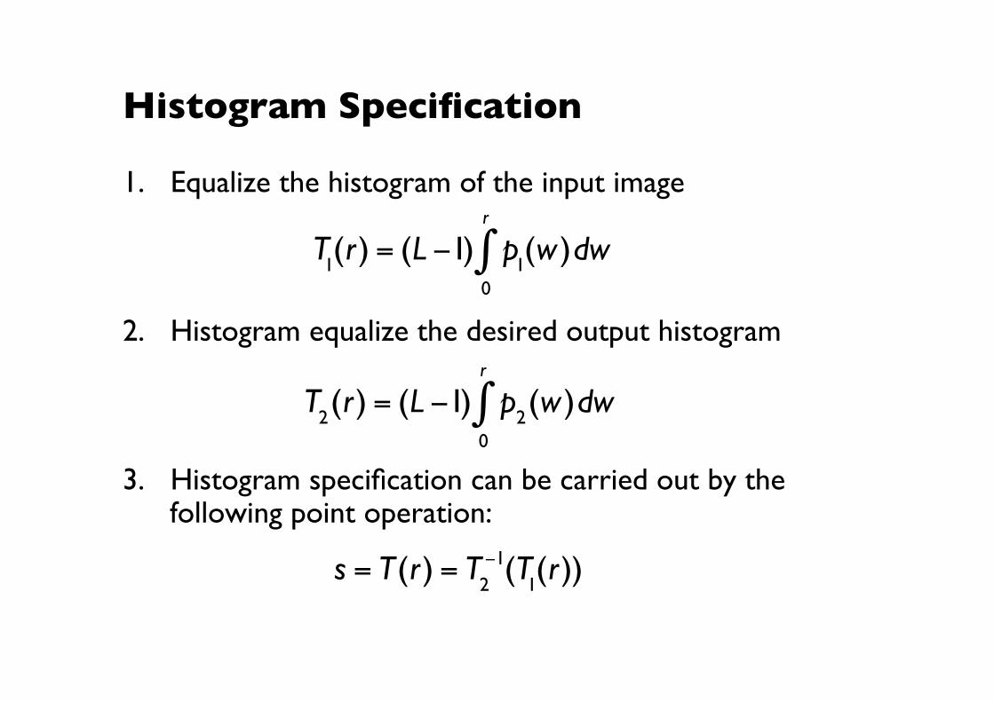
Histogram Specification

1.  Equalize the histogram of the input image

2.  Histogram equalize the desired output histogram

3.  Histogram specification can be carried out by the following point operation:

T1(r) = (L −1) p

1(w )dw

0

r

∫

T2(r) = (L −1) p

2(w )dw

0

r

∫

s = T(r) = T2−1(T

1(r))

Next week

•  Spatial filtering

Point Operations Histogram Processing

Documents