Point approximation of a space-homogeneous transport equation

Numer. Math. 56, 763-774 (1990) Numerische Mathematik �9 Springer-Verlag 1990

Point Approximation of a Space-Homogeneous Transport Equation

Santa Motta 1, Giovanni Russo 1, Hardy Moock 2, and Joachim Wick 2 Dipartimento di Matematica, Citt/t Universitaria, Viale A. Daria 6, 1-95t25 Catania

2 University of Kaiserslautern, Kaiserslautern, Federal Republic of Germany

Summary. We present an approximation method of a space-homogeneous transport equation which we prove is convergent. The method is very promising for numerical computation. Comparison of a numerical computation with an exact solution is given for the Master equation.

Subject Classifications: AMS(MOS): 45K05; 65C20; 82A70; CR: G1.8.

1 Introduction

We consider an one-dimensional, space-homogeneous transport problem in peri- odic geometry. This problem arises from a strong simplification of a model equation for semi-conductors. In the past a drift-diffusion approach was used in the computation of semiconductors [11, 13]. But this model is not satisfactory for the next generation of devices, since the assumption of thermodynamical equilibrium is not longer true. A better description for this case can be given by a kinetic model [16]. Here we consider only the electrostatic case

8f f_V.~x + Of (i) 8~- E.-~=SQ(k, k'){f(t, x, k ' )- f( t , x, k)} dk'

v=g(k), div E= S f (t, x, k) d k-n( t , x).

The 1.h.s. is similar to the Vlasov equation in plasmaphysics, which is treated numerically using particles [i, 6, 9]. The r.h.s, is similar to a collision term in linear transport theory, where completely different methods are used [4, 7]. Our aim is to extend the particle method to (1). Since the situation for the Vlasov-part is well-known, we have concentrated ourself to handle the collision term. We consider (1) in the space homogeneous case with a more general collision term. For this purpose let be Ti~-[0, 1] ~ the j-dimensional torus P, Q: T2 ~ IR +, T> 0 and f : [0, 7] x T1 ~ ]R § the integrable solution of

(2) 8 f (t, k)= S P(k, k')f(t, k ' )dk ' - f ( t , k) ~ Q(k, k')dk', 8 t rl rl

764 s. Motta et al.

where f (0 , k)=fo(k ) with ~ fo(k)dk= 1, is given. TI

For P = Q we get the space-homogeneous case of (1). In addition we require

(3) P(k, k')df(k)= ~ Q(k', k)df(k)=: G(k')e Lip, for a l l f e C ~. TI T1

Then (2) is a conservation equation

d f f(t , k)d k = ~ P(k, k')f(t, k')d k'd k - ~f Q(k, k')f(t, k)d k'd k d t rt T2 T2

= ~ {P(k, k')-Q(k', k)}f(t, k')dkdk'=O. T2

The Eq. (2) is similar to the master equation in the theory of stochastic processes. In this context Nanbu [13] has given a scheme, where the path of the particles is described by a stochastic difference equation. We will compare the numerical results of this stochastic method with those obtained with our deterministic one.

An other deterministic approach has been given in [12] and [15]. We have also implemented this method on a computer [3] and include here some numerical results.

The plan of the paper is the following. In w 2 we describe the method. In w 3 we show the convergence of the Euler scheme; in w 4 we show the convergence of the discrete approximation; in w 5 we apply the method to the space-homogeneous master equation and we compare our numerical results with the exact solution. Finally in w 6 we draw some conclusions.

2 The Method

We discretize (2) with respect to the time t with the timestep A t and indicate the time-levels by superscripts

(4) ff+~(k)=ff(k)(1--At ~ Q(k, k')dk')+ At ~ P(k, k')ff(k')dk' T~, T1

where fn is non-negative, as will be shown in Chap. 3. For this and the conservation property we can interpret fn as a density function of a probability-measure /z ", which can be approximated by a discrete measure. In contrast to the situation in plasmaphysics a discrete measure is not preserved by (4), since the gain term

P(k, k')f"(k')dk' creates a continuous part. Therefore after each time step TI

we must approximate the new measure by an appropriate discrete one.

Point Approximation of a Space-Homogeneous Transport Equation 765

We define for the initial measure/~o an approximation

o i N # N = ~ ~= 6(k-k~

by

i t9 - - = I d/2~ i = 1(1) N

(5) N o

Then we define by application of (4)

(6) v ~ t ~ Q(k, k')dk')#~ I P(k, k') p~ TI TI

which contains a discrete and an absolutely continuous part. In order to built an approximation of v ~ we use the following procedure:

Compute ki via

i k,

(7) ~ - = f dv ~ 0

and then k~ from k,

(8) k~=N f kv~ k , - 1

i=O(1)N

i=I (1)N.

The new k-values are the mean values of the [kl- 1, ki]-intervals. We now extend the definitions (6), (7) and (8) to all time-levels.

3 The Convergence of the Euler Scheme

For an estimation of

we define

(9)

llf'[I "= j" Iff(k)l dk Tl

Then it holds

G(k)..= ~ Q(k, k')dk'= ~ P(k', k)dk'. T1 T1

llf~+~ll < ~ ] l - d tG(k)] Iff(k)[ d k + A t I[P( k, k') f~(k')l dk' d k TI T2

< I]I-A tal[oo II fnll +AtllGllo~ II f"ll

<[li+2AtGl[~o [l f"l[.

766 s. Motta et al.

From the last inequality follows

IlffII~tII+2AtGII~ [I f~

IIf~ exp(ll 1 +2 TGII J .

Now we compare the Euler-solution (4) with the true solution of (2) at t, = nAt.

f"+ l ( k ) - f (t.+ ~, k)=f"(k) - f (t,, k) tn+ l

+ f I P(k,k'){f"(k')-f(v,k')} dk'dz tn T1

In+ I

-- I ~ Q(k, k'){f"(k)-f(z, k)} dk' dz tn T1

Zn+ 1

llf " + ~ - f ( t . + ~)[1 __< [If"-f(t.)l[ +2 S ~ G(k) [f"(k)-f(% k)[ dk dz In T1

in+ 1

<l l f" - f ( t . ) [ [ + 2 f ~ G(k)]ff(k)-ff+~(k)[ dkdr tn T1

tn+ 1

+ 2 f f G(k)[f"+~(k)-f (z ,k)[ dkdz tn T1

< ilf"-f(t.)ll +2A t 2 f G(k)IP(k, k')f"(k') T2

-Q(k, k') f"(k)[ dk' dk tn+ 1

+ 2 I I G(k)]f"+~(k)--f(Lk)I dkdz tn T1

< IIf"-f(t,)[I +2A t 2 ~ { S (G(k') P(k', k) T1 T1

+ G(k) Q(k, k')) dk'} [/"(k)] dk

trz+ l

+ 2 ~ [[G[[~ []f"+~-f(z){[ dz tn

/n+ l

< Nf"--f(t,)[] + 2 C ]If"l[ A t2+2 S [IGll ~o [[f"+1 -f(z)lt dz. tn

Here and in the sequel we use Co, C, C', ... to indicate constant factors in the estimations.

From Gronwall 's Lemma follows

Ilf "+1 - f ( t . + 0] [ <(]]f"-f(t.)][ +CoAt 2) exp(2 I]G]]~ A t)


and finally

since

IJf"-f(t.)lJ ~ Jlf ~ exp(C' nA t) + Co A t 2 ~ exp(C' yA t)

< [1 fo -f(to)I[ exp(C' t.) + C A t exp(C' t.)

= 1 A t exp(C'A t)(exp(C' t . ) - 1) d t 2 ~ exp(C'TA t) C' - t = l

C'A t exp(C'A t ) - 1

This shows the convergence of the Euler-scheme (4). If 1 - A t G(k)>O the Euler-Scheme conserves the non-negativity and

convergence transfers this to (2). the

4 The Convergence of the Discrete Approximation

To show the convergence of the discrete approximation of the measure v} in (6) for all time-levels we introduce the following.

Definition: Let be

U:={qS: T~ ~ [-0, 1]: 14)(x)-dp(y)l<=min(lj+x-yl)} j e Z

and M1 the set of the probability measures on Tt. Then for #, vcM~ we define

p(#, v):=sup Ifq6dft-lqbdvl. ~bEU

We call a sequence {VN}N~N c M1 (weakly) convergent to v, if lim p(vN, v)= 0. N~oo

Remarks. 1) p is the well-known bounded Lipschitz distance [2, 8] on a torus geometry.

2) Our definition of (weak) convergence coincides with the normal one defined by

lira f~dvN=~4~dv forall cI)eC~ N-~oO

In Chap. 2 we have described an algorithm which can be used to obtain succes- sively {/1}}.=o(1), o.

Now we wish to estimate p(#"+ 1, #~+ 1). From the triangle inequality follows

( lo) p(~," + ', ~4, + ~)<p(#"+ ~, v~)+p(v~, ~+ ~).

768 s. Motta et al.

We consider both terms of (10) separatly

p (/~" + ', v~v) = sup I 4)eU TI

+AtS T2

=sup I f d~eU TI

+At~ T1

0(k)(1 --A t I Q(k, k') dk')(#"(dk)-#"N(dk)) Tl

O(k) n(k, k')(l~"(dk')-p~(dk')) dk[

{0(k ) (1 -At ~ Q(k, k')dk') T,

O(k') n(k', k) dk'} (#"(dk)- #~(dk))].

We define

7t(k):=O(k)(1-A t ~ Q(k, k')dk')+At I O(k') P(k', k)dk' T1 T1

A :=max { 7t (k), ke T,}

B:=max (1, the smallest global Lipschitz-constant of 1 ~ i n T 0 .

It follows directly A <(l + 2At llG[Ioo)

and since Ge Lip, and 0 e U we get

17 ' (k0 - 7'(x2)l_-<10(k,)-0(k2)l+A t0(k , ) [ I Q(k,, k') TI

-Q(k2, k')dk'l+ A t [O(k,)-O(k2)[ ~ Q(k2, k')dk' T~

+A t I ~ O(k')(P(k', k,)-P(k', kz))dk'] TI

<=[k,-k2[+ A tL]k,-k2[+ At IIGI[~ [kl-k2[+ A t Lc, lki-k2[.

Where L'.= [[G'IIoo and L~b is the Lip-constant of S O(k')V(k', .)dk'. TI

Therefore it exists a constant C, such that

AB<I+CAt.

1 Now, ~ ~/" �9 U and

(11) P(#"+I'v})<AB ~ L gJ(k)(l~"(dk)-#}(dk))

< ( i + c,~ t) p(se, ~70.


For the second term of(10) it holds

p(vT~, #~+ ')=sup I ~ ~b(k) v~(dk)- ~ dp(k) #~+ '(dk)l OeU T1 TI

= sup I I dp(k) v~(dk)- O(k7 + ~) CeU TI i

=sup r v~(dk)- k7 + x) CeU i = k t - I l = l

with k0 = 0 and kN = 1. Using the mean value theorem:

N kt | N

p(v~v, bt~v+1)----sup ~ @(K',) I v}(dk)-N ~ O(kT+ ') " CeU ~=1 k , - I i = 1

The values K'i are contained in the [k~_ ,, k J-intervals. Furthermore we have:

1 N , k n + 1 p(v~,,#~v+l)=sup ~-~ ~ c~(Ki)-~( i )

CeU Iv i = 1

=<sup i) ~b(i 1)1 q~eU i = 1

_-< sup [ K}-- k7 + OeU i =

<sup [ki-, -k , ] ~eU i -

1 < - - : N "

Together with (11) we have now:

1 p(#,+ 1, #Tv+ 1)<(1 +CA t) p(p", #~,)-~ N

and by iteration

1 p(%~+ ~, #~+')~(1 + CA t) ~+~ p(#o, i~o)+~ ~ (1 + CA ty.

N v = 0

770 S. Motta et al.

Let be t=nA t, te[O, 7] then

p (~", ~4) < (1 + c A t)" p (ito, ~,o) + ~_ ( 1 + C A t)n 1

CAt

Since (1 + C A t)" < exp (C t) < exp (C 7), we showed convergence, if N ~ ~ . We summarize this in the

Theorem. Let be Tj-~[0, 1] j the j-dimensional torus, P, Q: T2"-"r~ + functions with

S P(k, k')df(k)= ~ Q(k, k')df(k)e Lip1 for al l fe C 1. T1 T~

Then the approximation P"N defined by (6), (7) and (8) converges to It", where p"(dk)=f (t, k)dk and f is the solution of

3,f= ~ P(k, k')f(t, k') dk ' - f ( t , k) ~ Q(k, k') dk' T1 T1

f(O, k)=fo(k)>O, Ifo(k) dk= 1 T1

for every finite time interval, if A t --, 0 and N A t ~ oe, provided lim/~o =#o. N~oo

5 Numerical Examples

First we consider the space-homogeneous master-equation [14]

(12) 3g (t, v)= ~o cxp(-(v--v')2)(g( t, v')-g(t , v))dv'. Ot

- - c t 3

Of course, this does not fit in our frame, since the domain in v is unbounded. But with the transformation

v 2k 1 & k . . . . v = - - k e ( - ~ , ~ ) 2 ( l + l v l ) ' 1 - 2 1 k I '

dk 1 dv 2 d~"=2(1 + Ivl) 2 ' d k - ( 1 - 2 l k l ) 2

(12) changes in the desired form. To do this, we multiply (12) with 2( t+lvl) 2 2k'

and substitute v ' - 1 - 2 [k't' then we get

O~g (t,v)'2(l+lv[) 2= f 2(l+lv[)2exp - v (13) c3 t - 1/2

2dk' 2k' )_g(t ,v))(1 Ik'[) 2" .(g(t, 1 - 2 {k', - 2


0 8

~06 g

O2

-20 -16 -1.2 -O.t, 0 K

i i i i

0'4 08 1~2 lt6 20

Fig. 1

Fig.

0.8

-20 -16 -12 -08 -0t~ 0g 08 12. 16 20

2k If we transform v = - - and call

1-21kl

2k ) 2 f ( t ,k ) :=g t, 1-21kl "(1-21kl) 2

n(k, k' ) . '=( l_2lkl) 2 exp - 1 - 2 l k l 1 - 2 1 k ' l ] ]

then (12) reads as

1/2 Of (t, k)= f Ot - 1 / 2

P(k, k')f(t, k') d k ' - i/2

I - - 1 / 2

P(k', k)f(t , k) dk'.

772 S. Motta et al.

0 8

06

~ 0 ~

. ~ . . . . . ~ t . ~ . . . ~ - I ~ ' I 0.2

-2.0 -1.6 -12 -08 - 0 ~ 0 / * 08 12 16 20

K

Fig. 3

08

06

J

-2.0 -1.6 -12 - 08 - 0 ~ o

K

Fig. 4

0~ 08 12 16 20

0.8

06

u-O~,

-20 -16 2 - 0 8 -OJ. ' 0 ' t , ' 0'.8 ~ ' ' 1~ 12 6 2O

Fig. 5


-2

08

06

02

-16 -12 - 08 -0~, 0

K

Fig. 6

0~ 08 12 16 20

The computation of the k~ according to (7) is done by a separate consideration of the discrete and the absolutely continuous part of vTv (cf. 6). For the discrete part the computation is easy. For the absolutely continuous part we use linear interpolation for a fast computation.

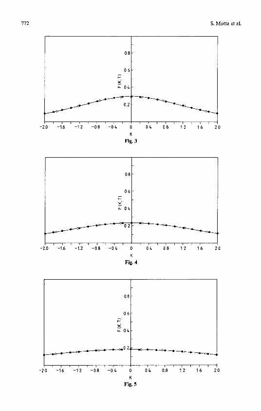
For the numerical computation we have chosen N=127, At=0.1. The Figs. 1-6 shows the results for t=0 , 2, 4, 6, 10, 20 where the lines indicate the true solution and the dots the numerical results, which were obtained by a suitable "linear weighting technique". The percentage error with respect to the exact solution is less then 2%. The circles indicate the results from Geyer [3]. He deals with 20 weighted particles, where the weights come from a Gaus- sian integration formula and a timestep A t = 0.05. The error and the computation time are comparable to our scheme.

Our computation time is about 40 s on a Siemens 7590.

6 Conclusion

We presented a point approximation method of a space homogeneous transport equation. The method is convergent and its computer implementation looks very promising. Results with a relative error less than 2% with respect to an exact solution were obtained only with 127 particles against the 10000 particles of Nanbu [14]. The extension to higher dimensions needs a proper approximation of v~v (cf. 6). In principle this can be done by a technique of Hlawka and Miick [5]. We are working to speed up this method.

R e f e r e n c e s

1. Birdsall, C.K., Langdon, A.B.: Plasma physics via computer simulation, I st Ed. New York: McGraw-Hill 1985

774 S. Motta et al.

2. Dudley, R.M.: Probabilities and metrics. Lecture Notes Series Mathematical Institut Aarhus 1976

3. Geyer, T.: Ober die Implementierung eines deterministischen Partikelverfahrens zur linearisierten Boltzmanngleichung. Kaiserslautern, Diplomarbeit 1987

4. Greenberg, W., van der Mee, C., Protopopescu, V.: Boundary value problems in abstract kinetic theory, 1 st Ed. Basel: Birkh/iuser 1987

5. Hlawka, E., Miick, E.: Qber eine Transformation yon gleichverteilten Folgen II. Computing 9, 127-138 (1972)

6. Hockney, R.W., Eastwood, J.W.: Computer Simulation using Particles. 1 st Ed. New York: McGraw-Hill 198t

7. Kaper, H.G., Lekkerkekker, C.G., Hejtmanek, J.: Spectral methods in linear transport theory, 1 st Ed. Basel: Birkh/iuser 1982

8. Kellerer, H.G.: Markov-Komposition und eine Anwendung auf Martingale. Math. Ann. 198, 99-122 (1972)

9. Kress, R., Wick, J.: Mathematical methods of plasmaphysics. Proc. of a Conference in Oberwolfach, Lang 1979

10. Kuipers, L., Niederreiter, H.: Uniform distribution of sequences, 1st Ed. New York: Wiley 1974 11. Markowitch, P.A.: The stationary semiconductor device equations, computational microelectron-

ics, 1 st Ed. Berlin Heidelberg New York: Springer 1986 12. Mas-Gallic, S.: A deterministic particle method for the linearized Boltzmann equation. Transp.

Theory Stat. Phys. 16, 855-890 (1987) 13. Mock, M.S.: Analysis of mathematical models of semiconductor devices, I st Ed. Dublin: Book

Press 1983 14. Nanbu, K.: Stochastic solution method of the master equation and the model Boltzmann equation.

J. Phys. Soz. Jpn 52, 2654-2658 (1983) 15. Niclot, B., Degond, P., Poupand, F.: Deterministic particle simulations of the Boltzmann transport

equation of semiconductors. Internal Report, Ecole Polytechnique 157, Polaiseau 1987 16. Ziman, J.: Principles of the theory of solids. Cambridge University Press 1972

Received April 13, 1988/March 14, 1989

Point approximation of a space-homogeneous transport equation

Documents