PNiQ: Integration of queuing networks in generalised stochastic Petri nets

PNiQ: Integration of Queuing Networks inGeneralized Stochastic Petri Nets

Matthias Becker and Helena SzczerbickaFB3/Computer Science, University of Bremen

P.O. Box 330440, 28334 Bremen, Germany.Email: matthias,[email protected]

Abstract. We combine generalized stochastic Petri nets (GSPN) and queuing networks at themodeling level by defining Petri Nets including Queuing Networks (PNiQ). The definition isespecially designed to allow approximate analysis by aggregation of the queuing nets andreplacing them with GSPN elements. Usually the aggregation of combined GSPN and queuingnetwork models is carried out manually which limits the use of this technique to experts andfurthermore may easily lead to modeling errors and larger approximation errors than inherent inthe method. This is what we want to avoid by the definition of PNiQ which shows how toincorporate queuing networks into GSPN and provides interfaces between them. This makescombined modeling easier and less error-prone. Steady state analysis of the model can be carriedout automatically: queuing network parts are analyzed with eff icient queuing network-algorithmsfor large nets and replaced by GSPN subnets that model the delay of tokens in the queuingnetwork. The resulting GSPN can then be handled with state-of-the-art tools.

1 Introduction

Queuing nets are widely used for performance analysis of complex systems like computer ormanufacturing systems. Efficient analysis algorithms for large and multi -class systems have beendeveloped over the years. Queuing nets furthermore offer a concise graphical description of theservice station, queue plus queuing discipline and stochastic routing.

Unfortunately queuing nets lack the abili ty to model more complicated structures likeblocking/locking, fork/join, simultaneous resource possession and synchronization. Generalizedstochastic Petri nets (GSPN) are a formalism for both qualitative and quantitative analysis ofsystems. But the quantitative analysis of GSPN via continous time Markov chain (CTMC)suffers from state space explosion (especially for large multi -class systems). Some more efficientanalysis algorithms exist (which for instance avoid exploring the complete state space), howeverthey are limited to restricted classes of GSPN [1,2]. If queuing net-like structures includingqueuing discipline and stochastic routing are modeled with GSPN, the state space grows rapidlyand the resulting GSPN is graphically complex and non comprehensible. Therefore it is desirableto find a combination of GSPN and queuing network which benefits from advantages of bothformalisms for modeling and analysis.

In the following sections we shortly review the literature on combination of GSPN and queuingnetworks and give an overview of the notation of queuing networks and GSPN. Then Petri Netsincluding Queuing Networks (PNiQ) are introduced as well formally as by an example. PNiQallow general combined modeling of systems and use eff icient queuing net analysis algorithmsand notation where possible and GSPN notation where needed. In the last section results ofcomputations show the accuracy and the eff iciency of the approach, an outlook finishes thearticle.

)(: PbagTO →

)(: PbagTI →

R→TW :

)(: PbagTH →

2 Literature Overview

If a system cannot be modeled by queuing networks (for instance if fork/join operations have tobe modeled) the queuing network-model is often extended directly by a CTMC [3] or combinedwith GSPN, which offer a graphical description for such operations and allow automatedgeneration of the underlying Markov chain. There exist some examples for combination ofGSPN and queuing networks as solution for special modeling problems [4,5], mostly based onreplacing one type of net by a flow-equivalent. But no general definition of a combined netstructure is given, which would allow easy and correct modeling of other problems.

Bause developed Queuing Petri Nets [6], where in special places called queuing places a queuingdiscipline can be modeled, according to that tokens are being served. Different to our approachthe solution is exact, based on the solution of the derived CTMC, therefore the complexity oflarge models still remains a problem. Neither queuing net algorithms for analysis nor thegraphical description of queuing networks are exploited.

3 Basic Notation

3.1 Queuing Networks

In this section we give a short description of queuing networks and provide as much of thenotation as is needed for our approach.

A queuing network [7]consists of N basic queuing systems which are the nodes in the graphicaldescription. Each queuing system consists of a waiting room and a server. The jobs waitaccording to a queuing discipline for being processed at the server. The service time is a randomvariable. Between the nodes routing probabiliti es p(i,j) are defined, which denote the probabili tythat a job that just has finished service at node i will next proceed to node j. The routingprobabiliti es of every node i must sum to one, i.e.∑ =

jjip 1),( for all i.Routing probabiliti es are

represented by weighted arcs. iλ denotes the throughput at node i, that is the mean rate with

which jobs leave node i in steady state. λ is the throughput of the whole queuing network. Thevisit ratio of node i is defined as: λλ /: iie = .The visit ratios can be calculated from the routing

probabiliti es. Plenty of eff icient analysis algorithms for the steady state solution exist [8].

3.2 GSPN

We now give the basic notation of a GSPN (cf. [9]). A GSPN is a tuple

where

• P is the set of places.

• T is the set of timed and immediate transitions.

• is the input function (represented by arcs from places to transitions).

• is the output function (represented by arcs from transitions to places).

• is the inhibition function (circle-headed arcs from places totransitions).

• defines the negative exponentially distributed firing rate in case of timed

),,,,,,,( 0mWHOITP Π

N→Π T:

N→Pm :0

Sqni ∈

},...,{ ,0, ikiii qqQ =0,iq 1+ik iqn

transitions and the weight in case of immediate transitions.

• is the priority function. Timed transitions have priority level 0, immediatetransitions have a priority level >0.

• is the initial marking.

The firing semantics of the transitions allows the modeling of fork/join, synchronisation,preemption etc. The analysis is mainly based on the solution of the derived CTMC, for detailssee [9].

4 Combined Modeling

The goal of this work is to provide a formalism for the aggregation of queuing nets in GSPN andthereby help to avoid modeling errors. With PNiQ combined modeling and analysis of generalsystems is possible for modelers without prior knowledge of the concept of aggregation.Informally a PNiQ is a live and bounded GSPN extended by a third node type, which representsmono-class queuing networks consisting of a number of queues. Tokens from the GSPN canenter a queuing network from transitions one by one and only at one specific queue called theinput queue of a queuing network. Tokens in one queuing network can move from queue toqueue within this net or to places of the GSPN or to input queues of other queuing network.Inhibitor arcs can as well be input or output arcs of a whole queuing network.

In the next section the formal definition of a PNiQ is given and afterwards the concept isexplained by means of an example.

4.1 Definition of a PNiQ

A PNiQ is a tuple ),,,,,,,,( 0mWHOISTP Π where

• P is the set of places.

• T is the set of transitions.

• S is the set of mono-class queuing nets.Each queuing net consists of

• a set of queues ,is called input queue, is the number of queues in .

A queue is specified by its queuing discipline and the service –time distribution.

• },...,1{ 0,0 SiqQ i == is the set of all i nput queues.

• ii QQ �= is the set of all queues.

• iyixii qnqqyxp ∈,, ,);,( are the routing probabiliti es within iqn .

)(,);,( ,o

ixii QPpqnqpxp ∪∈∈ are the routing probabiliti es that a job leaves

iqn after service at queue xiq , and moves into place or input queue p.

ir is the number of queues from which tokens can leave iqn . These queues arerefered as output queues.

• )(: PbagTI → is the input function (arcs from places to transitions).

• 0)(: QPbagQTO ∪→∪ is the output function (represented by arcs from transitions andqueues to places and input queues).

• )(: SPbagSTH ∪→∪ is the inhibition function (circle-headed arcs from places orqueuing nets to transitions or queuing nets).

• R→TW : defines the negative exponentially distributed firing rate in case of timedtransitions and the weight in case of immediate transitions.

• N→∪Π QT: is the priority function. Timed transitions and queues have prioritylevel 0, immediate transitions have a priority level >0.

• N→∪ SPm :0 is the initial marking. The initial marking of a queuing network is

defined as the initial total number of tokens in the queuing network.

4.2 Remarks on the Definition

From the definition of the output function follows that arcs from transitions or queues to theinput queue have multiplicity one. That means that tokens from transitions or queues may enter aqueuing network one by one at only one queue, the input queue. From a queue a served tokencan proceed to only one destination out of several possibiliti es given by the routing probabiliti es.That is queues cannot double tokens in the sense that for one served token two tokens are sent todifferent destinations like transitions can do. Furthermore it follows that arcs from queues toplaces have two labels, the arc multiplicity and the routing probabili ty. If such an arc has amultiplicity greater than one then for every token which leaves the queue to a place a number oftokens according to the multiplicity is placed in the destination place.

The explanation of the semantics of the inhibition function is the following: If an inhibitor arcfrom a queuing network to a transition exists then the transition can only fire if the totalpopulation of the queuing network is strictly below the arc multiplicity of the inhibitor arc. If aqueuing network is inhibited by an inhibitor arc then no token in the queuing network can bemoved, every action within the queuing network is inhibited.

The initial marking of a queuing network denotes the initial total population of the queuingnetwork. The initial distribution of these tokens on the queues of one queuing network is notrelevant for the behaviour of the PNiQ.

Some arcs are forbidden by the definition of a PNiQ, e.g. arcs from a place to a queue, arcs froma queue to a transition and inhibitor arcs from or to a single queue are not allowed.

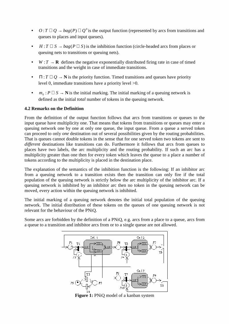
Figure 1: PNiQ model of a kanban system

4.3 Application Example of the Modeling Concept

Before presenting the analysis algorithm of the combined model an example from manufacturingis given for ill ustration of the modeling power. Figure 1 shows the corresponding PNiQ model ofa kanban system in its initial marking. The kanban system cannot be modeled with queuingnetworks because fork and join operations are required. When using GSPN to model the kanbansystem then only small systems can be studied due to state space explosion. The system consistsof three production cells. Within the system a number of pallets given in place P1 circulates. Weassume infinite supply of raw parts, therefore every palette in P1 means that a raw part is readyfor entering the line. In each cell buffer space is a limited resource. Kanbans (literally: cards)circulate within each cell and control the inventory: Whenever a palette wants to enter a cell , afree kanban must be available in the bulletin board (places P3, P4 and P10) of the cell . Onlywhen a free kanban (= token in bulletin board) is available, the kanban is attached to the paletteand the palette can enter the cell . The palette proceeds through the cell and when it leaves thecell , the kanban returns to the bulletin board. The production steps in each cell are modeled by aproduct form queuing network. Some palettes proceed through cell one and two and return to P1after the finished products are removed. In cell one a certain percentage of palettes leave cell oneand proceed to cell three, where the parts undergo a different final production step.

Because of the inhibitor arc from the queuing network of cell one transition T3 can only fire ifcell one is empty. In that case T3 is enabled and its firing inhibits any action in cell one by atoken in P6 until transition T4 fires. This models maintenance of cell one, which can only takeplace if this cell i s empty. During maintenance no parts can be processed in cell one.

5 Analysis

The structure of a PNiQ allows to perform eff icient quantitative analysis and also to usetechniques for structural analysis known from Petri nets. The combined model is transformedinto a pure GSPN in which the queuing network are substituted by GSPN subnets. These GSPNsubnets are said to be flow equivalent to the queuing network, because the subnet models thedelay that the flow of tokens experiences in the queuing network.

The flow equivalent GSPN subnet for a queuing network iqn consists of one input place iip ,

one output place iop , irr ,...,1= immediate routing transitions rirt , and one timed transition ifet

with marking dependent firing rates. The firing rates equal the throughput of the queuingnetwork with a certain population and depend on the number of tokens of the input place. Thenumber of tokens in iip represents the population of iqn . The tokens leaving iqn are gathered in

iop . They can leave the output place by immediate routing transitions rirt , whose weights are

adjusted according to the visit ratio and routing probabiliti es of output queue r.

The visit ratio of an output queue is the same for different populations of the queuing networktherefore the weights of routing transitions are not marking-dependent. Immediate transitions donot contribute to the number of tangible markings. Even if complex dependencies or controlstructures are modeled with immediate transitions in the GSPN part of a PNiQ this does notincrease the computational complexity as much as the complex graphical appearance of thisstructures might suggest.

The substitution of a subnet by a flow equivalent is only exact in product form nets but based onthe concept of near-independence the error of the substitution in non-product form nets will i sexpected to be small i n most cases.

One important restriction is the use of exactly one input queue in each queuing network. If the

arrivals from the outside GSPN into the queuing network could happen to different queues, thereplacement by only one input place and one flow equivalent transition would introduceadditional error because the mean waiting time in a common place would be less than it is indifferent input queues.

The next section shows formally how the substitution of the queuing network is done.

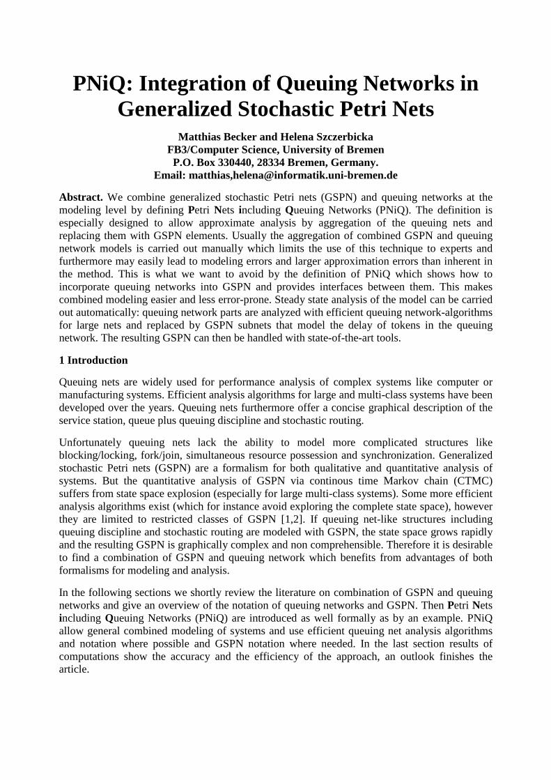
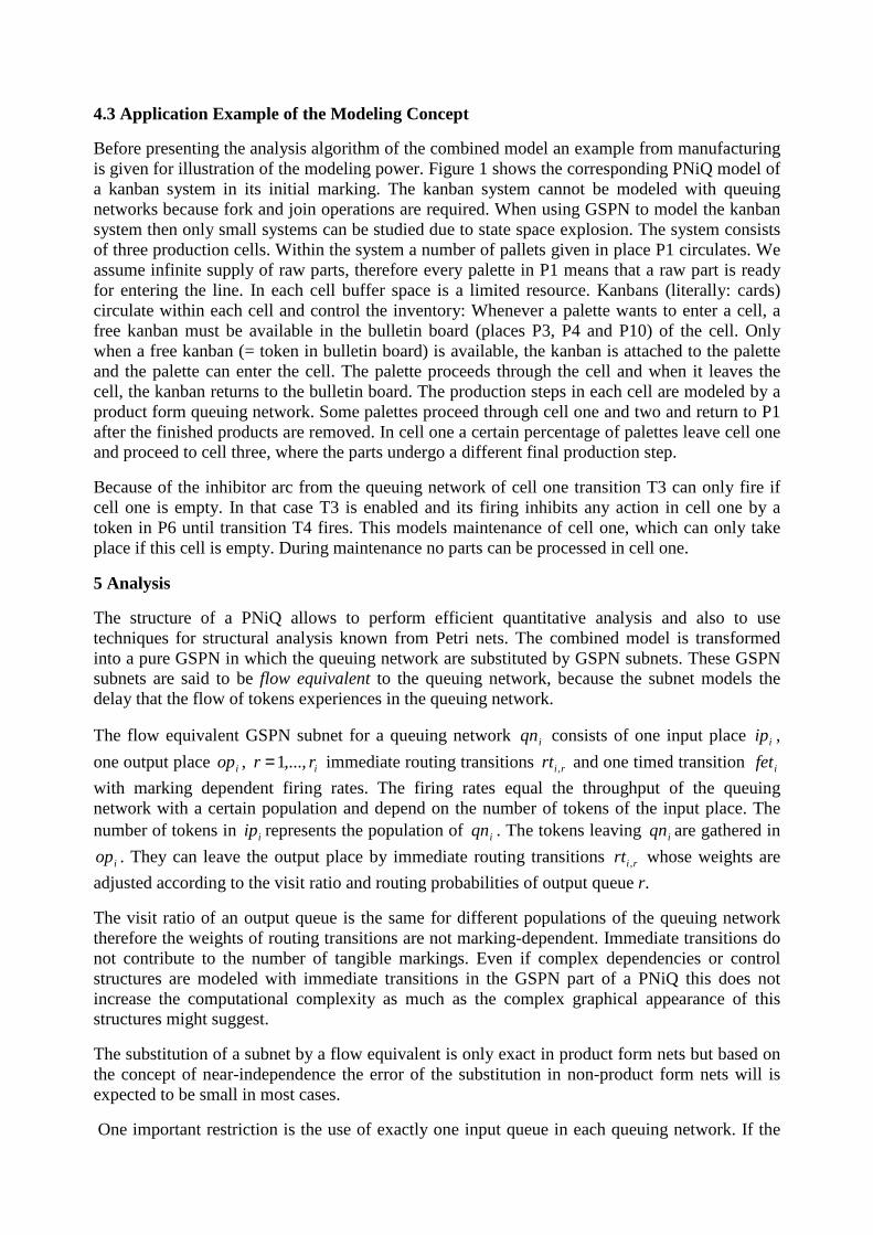
Figure 2: Transformed PNiQ

5.1 Transformation of a PNiQ into a GSPN

In order to solve the PNiQ for steady state, the GSPN PN' is derived from PNiQ),,,,,,,,( 0mWHOISTP Π by substitution of the queuing networks by GSPN elements:

),,,,,,,( 0mWHOITPNP ′Π′′′′′′′=′ with

• },...,1{},...,1{ SiopSiipPP ii =∪=∪=′ is the set of places extended by one input

place iip and one output place iop for each iqn .

• },...,1,,...1{},...,1{ , irii rrSirtSifetTT ==∪=∪=′ is the set of transitions extended by

one flow equivalent transition ( ifet ) and immediate routing transitions ( rirt , ) for each

iqn .

• },...,1,,...,1);,{(},...,1);,{( , iiriii rrSioprtSiipfetII ==∪=∪=′

• },),(),{(}),(),{(

},...,1),{(},,),(),{())}(({

,,0,,,

00,0,

PpOpqprtOqqiprt

SiopfetQqTtOqtiptPbagTOOO

ririiriiri

iiiii

∈∈∪∈∪

=∪∈∈∈∪×∈=′

• },),(),{(

}),(),{(},),(),{())}(({

TtHqntipt

HqnqnipfetPpHpqnpfetPbagTHHH

ii

jiiiii

∈∈∪

∈∪∈∈∪×∈=′

• R→′′ TW :The population dependent firing rate of ifet is:

iiii maxpopkSikkipfetW ,...,1,,...,1),()'#if,( ====′ λ where )(kiλ is the mean

throughput of iqn with a total population of k and imaxpop is the maximal population of

iqn .

The weights of the routing transitions are calculated according to:)();,()( 0

,,, QPppqpertW rrririri ∪∈=′ is the place or queue to which the tokens leave

from output queue riq , . (The calculation of rie , , )(kiλ and imaxpop is explained later.)

• Π′ is the priority function.

ijii kjSirtfet ,...,1;,...,1,1)(,0)( , ===Π′=Π′ .

• N→′′ Pm :0 is the initial marking.

Siopmqnmipm iii ,...,1,0)(),()( 000 ==′=′

Figure 2 shows the GSPN which is obtained by transforming the PNiQ of Fig. 1. In cell two andthree the two routing transitions could be replaced by one because the output place of the tworouting transitions is the same.

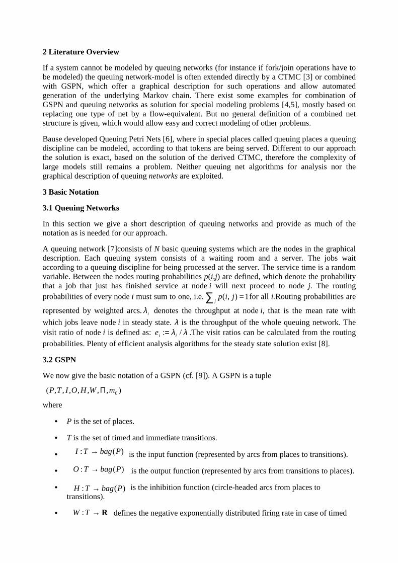
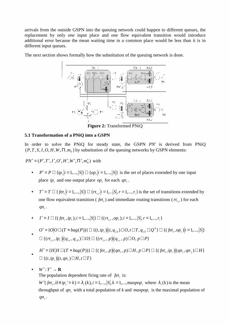
Figure 3: Illustration of the Analysis Algorithm

5.2 Analysis Algorithm

First the PNiQ is transformed into a GSPN PN' according to section 5.1 without the calculationof the weight function W'. Then the P-invariants of PN' are determined, which can be donewithout knowing W'. The maximal population of iqn is calculated from the P-invariants in

which ifet lies: }boundedk is whichinvariant,min{ −−∈= Pfetkmaxpop ii . Then each iqn is

analyzed in isolation as closed queuing network from population imaxpopk ,..,1= by short-

cutting iqn . Short-cutting means that a token that leaves iqn from an output queue, reenters

iqn immediately at the input queue 0,iq . This is done by setting the routing probabiliti es

),()0,( rii prprp = , for all output queues iri rrq ,...,1,, = , of iqn and )( SPpr ∪∈ . From the

analysis of the shortcut queuing network we get the population dependent throughputs )(kiλ of

each iqn and visit ratios jiqe

,of each queue iji qnq ∈, .Then the values of W' can be calculated

according to )()'#,( kkipiffetW iii λ==′ and ),()( ,,, rririri pqpertW =′ . PN' is now completely

defined and structural and quantitative analysis can be done with any tool which can handlepopulation dependent firing rates. Table 1 shows the complete algorithm and Fig. 3 gives anoverview of the analysis procedure.

Algorithm:

1. Transform PNiQ into GSPN NP ′ except W ′ .

2. Calculate P-invariants in NP ′ .

3. Set }boundedk is whichinvariant,min{ −−∈= Pfetkmaxpop ii .

4. Shortcut Siqni ,...,1, = and calculate ii maxpopkk ,...,1),( =λ and iji kje ,...,1,, = .

5. In NP ′ set )()'#if,( kkipfetW iii λ==′ for imaxpopkSi ,...,1,,...,1 == .

6. In NP ′ set ),()( ,,, rririri pqpertW =′ for ir krSiQPp ,...,1,,...,1),( 0 ==∪∈ .

7. Analyze NP ′ .

Table 1: Analysis Algorithm

Steady state analysis of PN' yields the throughput of transitions, the average population of placesand the probabili ty of f inding k tokens in place p, P )(# kp = . Therefore P )(# kipi = is the

probabili ty of f inding a population of k in iqn .

6 Results

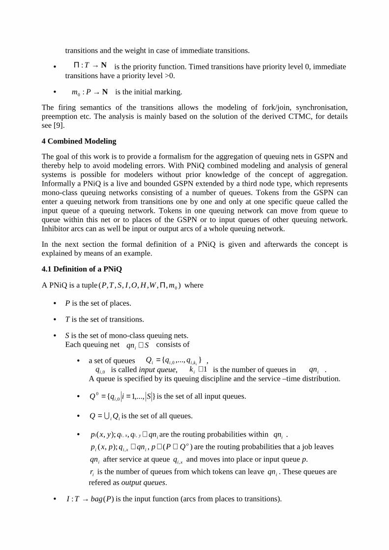
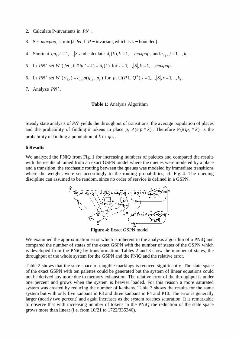
We analyzed the PNiQ from Fig. 1 for increasing numbers of palettes and compared the resultswith the results obtained from an exact GSPN model where the queues were modeled by a placeand a transition, the stochastic routing between the queues was modeled by immediate transitionswhere the weights were set accordingly to the routing probabiliti es, cf. Fig. 4. The queuingdiscipline can assumed to be random, since no order of service is defined in a GSPN.

Figure 4: Exact GSPN model

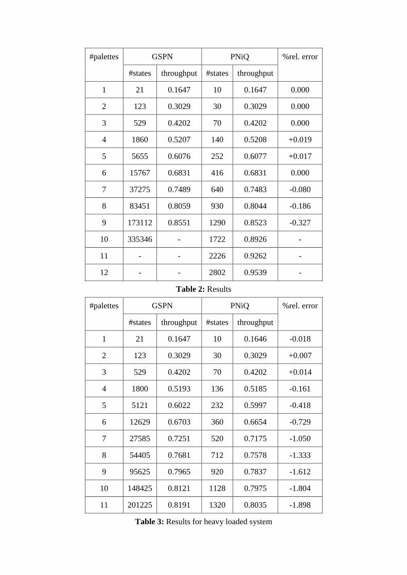
We examined the approximation error which is inherent in the analysis algorithm of a PNiQ andcompared the number of states of the exact GSPN with the number of states of the GSPN whichis developed from the PNiQ by transformation. Tables 2 and 3 show the number of states, thethroughput of the whole system for the GSPN and the PNiQ and the relative error.

Table 2 shows that the state space of tangible markings is reduced significantly. The state spaceof the exact GSPN with ten palettes could be generated but the system of linear equations couldnot be derived any more due to memory exhaustion. The relative error of the throughput is underone percent and grows when the system is heavier loaded. For this reason a more saturatedsystem was created by reducing the number of kanbans. Table 3 shows the results for the samesystem but with only five kanbans in P3 and three kanbans in P4 and P10. The error is generallylarger (nearly two percent) and again increases as the system reaches saturation. It is remarkableto observe that with increasing number of tokens in the PNiQ the reduction of the state spacegrows more than linear (i.e. from 10/21 to 1722/335346).

GSPN PNiQ#palettes

#states throughput #states throughput

%rel. error

1 21 0.1647 10 0.1647 0.000

2 123 0.3029 30 0.3029 0.000

3 529 0.4202 70 0.4202 0.000

4 1860 0.5207 140 0.5208 +0.019

5 5655 0.6076 252 0.6077 +0.017

6 15767 0.6831 416 0.6831 0.000

7 37275 0.7489 640 0.7483 -0.080

8 83451 0.8059 930 0.8044 -0.186

9 173112 0.8551 1290 0.8523 -0.327

10 335346 - 1722 0.8926 -

11 - - 2226 0.9262 -

12 - - 2802 0.9539 -

Table 2: Results

GSPN PNiQ#palettes

#states throughput #states throughput

%rel. error

1 21 0.1647 10 0.1646 -0.018

2 123 0.3029 30 0.3029 +0.007

3 529 0.4202 70 0.4202 +0.014

4 1800 0.5193 136 0.5185 -0.161

5 5121 0.6022 232 0.5997 -0.418

6 12629 0.6703 360 0.6654 -0.729

7 27585 0.7251 520 0.7175 -1.050

8 54405 0.7681 712 0.7578 -1.333

9 95625 0.7965 920 0.7837 -1.612

10 148425 0.8121 1128 0.7975 -1.804

11 201225 0.8191 1320 0.8035 -1.898

Table 3: Results for heavy loaded system

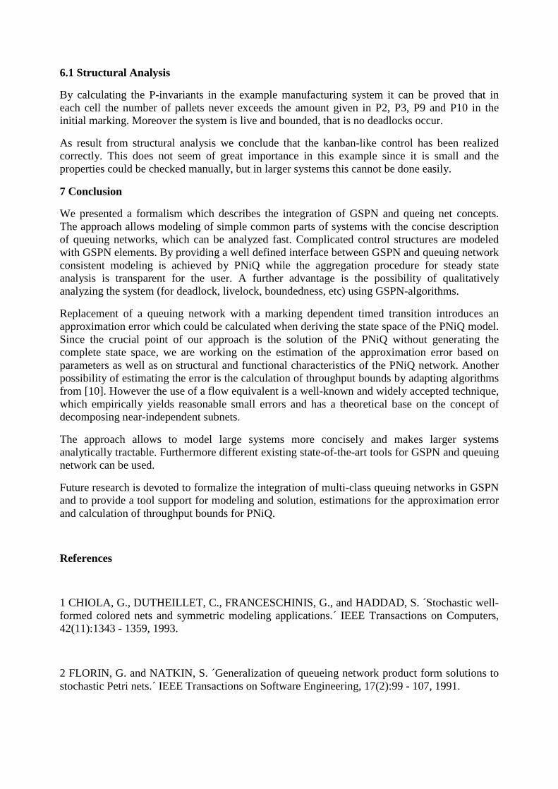
6.1 Structural Analysis

By calculating the P-invariants in the example manufacturing system it can be proved that ineach cell the number of pallets never exceeds the amount given in P2, P3, P9 and P10 in theinitial marking. Moreover the system is li ve and bounded, that is no deadlocks occur.

As result from structural analysis we conclude that the kanban-like control has been realizedcorrectly. This does not seem of great importance in this example since it is small and theproperties could be checked manually, but in larger systems this cannot be done easily.

7 Conclusion

We presented a formalism which describes the integration of GSPN and queing net concepts.The approach allows modeling of simple common parts of systems with the concise descriptionof queuing networks, which can be analyzed fast. Complicated control structures are modeledwith GSPN elements. By providing a well defined interface between GSPN and queuing networkconsistent modeling is achieved by PNiQ while the aggregation procedure for steady stateanalysis is transparent for the user. A further advantage is the possibili ty of qualitativelyanalyzing the system (for deadlock, li velock, boundedness, etc) using GSPN-algorithms.

Replacement of a queuing network with a marking dependent timed transition introduces anapproximation error which could be calculated when deriving the state space of the PNiQ model.Since the crucial point of our approach is the solution of the PNiQ without generating thecomplete state space, we are working on the estimation of the approximation error based onparameters as well as on structural and functional characteristics of the PNiQ network. Anotherpossibili ty of estimating the error is the calculation of throughput bounds by adapting algorithmsfrom [10]. However the use of a flow equivalent is a well -known and widely accepted technique,which empirically yields reasonable small errors and has a theoretical base on the concept ofdecomposing near-independent subnets.

The approach allows to model large systems more concisely and makes larger systemsanalytically tractable. Furthermore different existing state-of-the-art tools for GSPN and queuingnetwork can be used.

Future research is devoted to formalize the integration of multi -class queuing networks in GSPNand to provide a tool support for modeling and solution, estimations for the approximation errorand calculation of throughput bounds for PNiQ.

References

1 CHIOLA, G., DUTHEILLET, C., FRANCESCHINIS, G., and HADDAD, S. ´Stochastic well -formed colored nets and symmetric modeling applications.´ IEEE Transactions on Computers,42(11):1343 - 1359, 1993.

2 FLORIN, G. and NATKIN, S. ´Generalization of queueing network product form solutions tostochastic Petri nets.´ IEEE Transactions on Software Engineering, 17(2):99 - 107, 1991.

3 DE ARAÚJO, S. L., FREIN, Y., and DI MASCOLO, M. ´Efficient procedures for the designof kanban systems.´ International Conference on Industrial Engineering and ProductionManagement, 1993.

4 BALBO, G., BRUELL, S.C. and SUBBARO, G.´Combining queueing networks andgeneralized stochastic Petri nets for the solution of complex models of system behavior´. IEEETransactions on Computers, 37(10):1251 -1268, 1988.

5 SZCZERBICKA, H. ´A combined queuing network and stochastic Petri-net approach forevaluating the performabili ty of fault-tolerant computer systems.´ Performance Evaluation,14:217 - 226, 1992.

6 BAUSE, F. ´Queueing petri nets: A formalism for the combined qualitative and quantitativeanalysis of systems.´ In Proceedings of the International Workshop on Petri Nets andPerformance Models, pages 14-23, Toulouse, France, October 1993. IEEE-Computer SocietyPress.

7 KLEINROCK, L. ́ Queueing Systems Volume I: Theory.´ John Wiley & Sons, 1975.

8 STEWART, W.J. ´Introduction to Numerical Solution of Markov Chains.´ Princton UniversityPress, 1984.

9 MARSAN, M., BALBO, G.,CONTE, G.,DONATELLI, S., and FRANCESCHINIS, G.´Modelli ng with Generalized Stochastic Petri Nets.´ John Wiley and Sons, Chichester England,1995.

10 CHIOLA, G.,ANGLANO, C.,CAMPOS, J.,COLOM, J. M., and SILVA, M. ´Operationalanalysis of timed Petri nets and application to the computation of performance bounds.´ InProceedings of the International Workshop on Petri Nets and Performance Models, pages 128-137, Toulouse, France, October 1993. IEEE-Computer Society Press.