PLS regression on wavelet compressed NIR spectra

Ž .Chemometrics and Intelligent Laboratory Systems 42 1998 209–220

PLS regression on wavelet compressed NIR spectra

Johan Trygg ), Svante WoldResearch Group for Chemometrics, Department of Organic Chemistry, Umea UniÕersity, Umea S-901 87, Sweden˚ ˚

Abstract

Today, good compression methods are more and more needed, due to the ever increasing amount of data that is beingcollected. The mere thought of the computational power demanded to calculate a regression model on a large data set withmany thousands of variables can often be depressing. This paper should be treated as an introduction to how the discretewavelet transform can be used in multivariate calibration. It will be shown that by using the fast wavelet transform on indi-

Ž .vidual signals as a preprocessing method in regression modelling on near-infrared NIR spectra, good compression isachieved with almost no loss of information. No loss of information means that the predictive ability and the diagnostics,together with the graphical displays of the data compressed regression model, are basically the same as for the original un-compressed regression model. The regression method used here is Partial Least Squares, PLS. In a NIR-VIS example, com-pression of the data set to 3% of its original size was achieved. q 1998 Elsevier Science B.V. All rights reserved.

Keywords: Discrete wavelet transform; Partial least squares projections to latent structures; Data compression; NIR spectroscopy; Pre-processing techniques

1. Introduction

The idea of representing a signal as the sum ofanalyzing functions dates back to the days whenJoseph Fourier presented his theories on the Fouriertransform in 1807. Wavelet transformation is no dif-ferent, it is a linear transformation and its trademarksare good compression and denoising of complicatedsignals and images. Wavelets look like small oscillat-ing waves, and they have the ability to analyze a sig-nal according to scale, i.e., inverse frequency. Thesize of the analyzing window in wavelet transformvaries with different scales, and it is this small but still

) Corresponding author. Fax: q46-90-13-88-85; e-mail:[email protected].

very important property, along with the fact thatwavelet functions are local in both time and fre-quency that makes the wavelet transform versatile anduseful.

The analyzing mother wavelet used in this paperis the popular Daubechies-4 wavelet function, whichforms an orthogonal set of basis functions. Wavelettransformation is becoming increasingly more popu-

w xlar in other fields 1,2 , and lately, there has been agrowing number of papers from the chemical societyw x3,4 , where it has been used as a feature extractiontool and for removal of noise. Good tutorials on the

w xwavelet transform have also been given 5,6,24 . Bosw xand Vrielink 7 have reported the use of the wavelet

Ž .transformation in the classification of infrared IRspectra. Alsberg has pointed out many applications

0169-7439r98r$19.00 q 1998 Elsevier Science B.V. All rights reserved.Ž .PII: S0169-7439 98 00013-6

( )J. Trygg, S. WoldrChemometrics and Intelligent Laboratory Systems 42 1998 209–220210

where wavelets could be useful, among those is thew x w xdenoising of IR spectra 8 . Walczak et al. 9 have

used wavelet packet transformation as a feature ex-traction tool for the classification of NIR spectra, andfor simultaneous noise suppression and data com-

w xpression of NIR spectra 6 .The main goal of this report is to present an easy

introduction to how the wavelet transform can be usedas an effective compression tool on NIR spectra foruse in multivariate calibration. NIR spectra are veryredundant by nature, and therefore, suitable for com-pression. Compressing a large data set with thewavelet transform and then performing regressionanalysis on some of the wavelet coefficients is fastcompared to calculating the PLS model on the origi-nal data set.

2. Overview of the wavelet transform

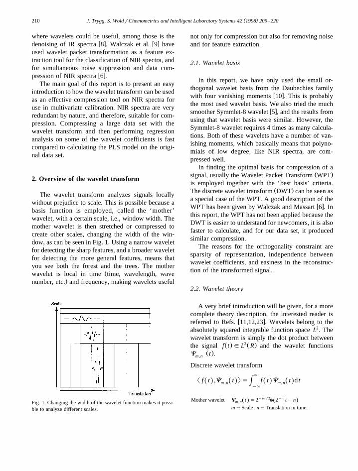
The wavelet transform analyzes signals locallywithout prejudice to scale. This is possible because abasis function is employed, called the ‘mother’wavelet, with a certain scale, i.e., window width. Themother wavelet is then stretched or compressed tocreate other scales, changing the width of the win-dow, as can be seen in Fig. 1. Using a narrow waveletfor detecting the sharp features, and a broader waveletfor detecting the more general features, means thatyou see both the forest and the trees. The mother

Žwavelet is local in time time, wavelength, wave.number, etc. and frequency, making wavelets useful

Fig. 1. Changing the width of the wavelet function makes it possi-ble to analyze different scales.

not only for compression but also for removing noiseand for feature extraction.

2.1. WaÕelet basis

In this report, we have only used the small or-thogonal wavelet basis from the Daubechies family

w xwith four vanishing moments 10 . This is probablythe most used wavelet basis. We also tried the much

w xsmoother Symmlet-8 wavelet 5 , and the results fromusing that wavelet basis were similar. However, theSymmlet-8 wavelet requires 4 times as many calcula-tions. Both of these wavelets have a number of van-ishing moments, which basically means that polyno-mials of low degree, like NIR spectra, are com-pressed well.

In finding the optimal basis for compression of aŽ .signal, usually the Wavelet Packet Transform WPT

is employed together with the ‘best basis’ criteria.Ž .The discrete wavelet transform DWT can be seen as

a special case of the WPT. A good description of thew xWPT has been given by Walczak and Massart 6 . In

this report, the WPT has not been applied because theDWT is easier to understand for newcomers, it is alsofaster to calculate, and for our data set, it producedsimilar compression.

The reasons for the orthogonality constraint aresparsity of representation, independence betweenwavelet coefficients, and easiness in the reconstruc-tion of the transformed signal.

2.2. WaÕelet theory

A very brief introduction will be given, for a morecomplete theory description, the interested reader is

w xreferred to Refs. 11,12,23 . Wavelets belong to theabsolutely squared integrable function space L2. Thewavelet transform is simply the dot product between

Ž . 2Ž .the signal f t g L R and the wavelet functionsŽ .C t .m ,n

Discrete wavelet transform`

² :f t ,C t s f t C t d tŽ . Ž . Ž . Ž .Hm ,n m ,ny`

Mother wavelet C t s2ym r2c 2ym tynŽ . Ž .m ,n

msScale, nsTranslation in time.

( )J. Trygg, S. WoldrChemometrics and Intelligent Laboratory Systems 42 1998 209–220 211

One of the mathematical restrictions that applies tothe wavelet:

The admissibility condition

ˆ 2< <` C vŽ .C s dv-`HC < <vy`

ˆ Ž .for finite energy C v s0 for vF0vsFrequencyˆ Ž .C v sFT on wavelet function.

2.3. Multiresolution analysis, MRA

In 1986, a fast wavelet transformation techniquecalled multiresolution analysis was presented by

w x nMallat 13 . The signal needs to be of length 2 ,where n is an integer. This poses no problems, be-cause the signal can be padded to the nearest 2 n. Inmultiresolution analysis, another function called thescaling function is introduced, which acts as a start-ing point in the analysis and makes it possible tocompute wavelet coefficients fast. From the waveletand scaling function, respectively, filter coefficientsare derived and used in the transformation, and are

Ž .implemented as finite impulse response FIR filters.These filter coefficients are put in a filter coefficientmatrix of size k) k, where k is the length of the sig-nal to be analyzed, and a pyramid algorithm is used.The filter coefficients are normalized to make surethat the energy on each scale is the same, and the

1normalizing constant is . Energy is defined as the'2

squared sum of all the coefficients. The scaling filterS is located on the first kr2 rows, and the waveletfilter D is located on the last kr2 rows. The filtermatrix is constructed by moving the filter coeffi-cients two steps to the right when moving from rowto row, requiring kr2 rows to cover the signal. Thenumber of filter coefficients depends on what waveletfunction is being used. The wavelet filter coefficientscan be derived from the scaling filter coefficients.

Ž . Ž . iWavelet coefficient cy iq1 s y1 . ScalingŽ .coefficient i , is1,2, . . . ,c where c is the number

of filter coefficients. The Daubechies-4 wavelet func-tion has the following four scaling filter coefficients

' ' ' '1q 3 3q 3 3y 3 1y 3w x, , , and wavelet filter coef-4 4 4 4

Ž . Ž .' ' ' '1y 3 3y 3 3q 3 1q 3w xficients ,y , ,y .4 4 4 4

Reconstruction of the original signal from thewavelet coefficients is straightforward, because we

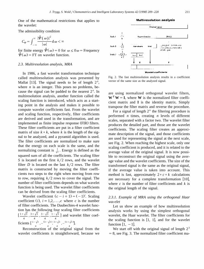
Fig. 2. The fast multiresolution analysis results in a coefficientvector of the same size as the analyzed signal.

are using normalized orthogonal wavelet filters,W T WsI, where W is the normalized filter coeffi-cient matrix and I is the identity matrix. Simplytranspose the filter matrix and reverse the procedure.

For a signal of length 2 n the filtering procedure isperformed n times, creating n levels of differentscales, separated with a factor two. The wavelet filterproduces the detailed part, and those are the waveletcoefficients. The scaling filter creates an approxi-mate description of the signal, and those coefficientsare used for representing the signal at the next scale,see Fig. 2. When reaching the highest scale, only onescaling coefficient is produced, and it is related to theaverage value of the original signal. It is now possi-ble to reconstruct the original signal using the aver-age value and the wavelet coefficients. The size of thetransformed signal is the same as the original signal,if the average value is taken into account. Thismethod is fast, approximately 2)c) k calculations

w xare necessary for a complete transformation 10 ,where c is the number of filter coefficients and k isthe original length of the signal.

2.3.1. Example of MRA using the orthogonal HaarwaÕelet

Let us show an example of how multiresolutionanalysis works by using the simplest orthogonalwavelet, the Haar wavelet. The filter coefficients for

w xthe scaling function is 1, 1 , and for the waveletw xfunction 1, y1 .

We start off with the original signal of length 23

s8, see Fig. 3. The normalized filter coefficient ma-


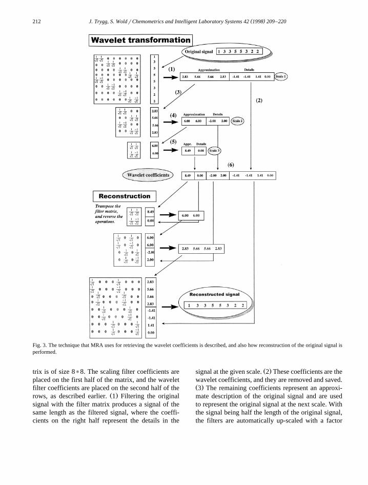
Fig. 3. The technique that MRA uses for retrieving the wavelet coefficients is described, and also how reconstruction of the original signal isperformed.

trix is of size 8)8. The scaling filter coefficients areplaced on the first half of the matrix, and the waveletfilter coefficients are placed on the second half of the

Ž .rows, as described earlier. 1 Filtering the originalsignal with the filter matrix produces a signal of thesame length as the filtered signal, where the coeffi-cients on the right half represent the details in the

Ž .signal at the given scale. 2 These coefficients are thewavelet coefficients, and they are removed and saved.Ž .3 The remaining coefficients represent an approxi-mate description of the original signal and are usedto represent the original signal at the next scale. Withthe signal being half the length of the original signal,the filters are automatically up-scaled with a factor


Ž .two, i.e., changing the width of the filter. 4 Thecoarse signal is then filtered with a reduced filter ma-trix. We repeat the procedure from the last scale, re-moving the right half of the coefficients as waveletcoefficients and using the other half to represent the

Ž .signal at the next scale. 5 With an even more re-duced filter matrix, the filtered output signal of lengthtwo consists of one wavelet coefficient and also the

Ž .normalized average value of the original signal. 6Both of these are put in the wavelet coefficient vec-tor. Now, we are done with the fast wavelet transfor-mation, and the wavelet coefficient vector can be usedfor a complete reconstruction of the original signal,by transposing the normalized filter coefficient ma-trix and reversing the filtering operations previouslydone. It is important to realize that the sum of thecoarse and the detailed signal at a certain scalematches the signal on the scale below, if this is notthe case, we would not be able to recover the origi-nal signal.

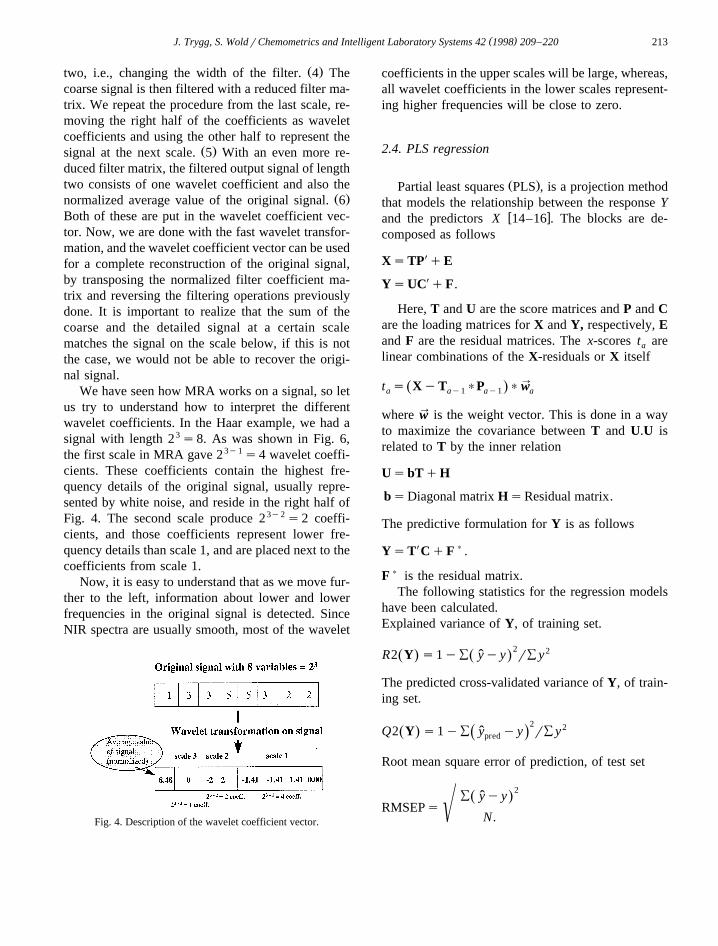
We have seen how MRA works on a signal, so letus try to understand how to interpret the differentwavelet coefficients. In the Haar example, we had asignal with length 23 s8. As was shown in Fig. 6,the first scale in MRA gave 23y1 s4 wavelet coeffi-cients. These coefficients contain the highest fre-quency details of the original signal, usually repre-sented by white noise, and reside in the right half ofFig. 4. The second scale produce 23y2 s2 coeffi-cients, and those coefficients represent lower fre-quency details than scale 1, and are placed next to thecoefficients from scale 1.

Now, it is easy to understand that as we move fur-ther to the left, information about lower and lowerfrequencies in the original signal is detected. SinceNIR spectra are usually smooth, most of the wavelet

Fig. 4. Description of the wavelet coefficient vector.

coefficients in the upper scales will be large, whereas,all wavelet coefficients in the lower scales represent-ing higher frequencies will be close to zero.

2.4. PLS regression

Ž .Partial least squares PLS , is a projection methodthat models the relationship between the response Y

w xand the predictors X 14–16 . The blocks are de-composed as follows

XsTPX qE

YsUCX qF.

Here, T and U are the score matrices and P and Care the loading matrices for X and Y, respectively, Eand F are the residual matrices. The x-scores t area

linear combinations of the X-residuals or X itself

™t s XyT )P )wŽ .a ay1 ay1 a

™where w is the weight vector. This is done in a wayto maximize the covariance between T and U.U isrelated to T by the inner relation

UsbTqH

bsDiagonal matrix HsResidual matrix.

The predictive formulation for Y is as follows

YsTXCqF ) .

F ) is the residual matrix.The following statistics for the regression models

have been calculated.Explained variance of Y, of training set.

2 2R2 Y s1yÝ yyy rÝ yŽ . Ž .ˆ

The predicted cross-validated variance of Y, of train-ing set.

2 2Q2 Y s1yÝ y yy rÝ yŽ . ˆŽ .pred

Root mean square error of prediction, of test set

2Ý yyyŽ .ˆRMSEPs(

N.


For a matrix X of size N) K , the variance vector iscalculated as

2Ý x yxŽ .nk kVariance sk Ny1

Ž . Žks1,2, . . . K column index , ns1,2, . . . N row.index .

2.5. Software

The software used for the wavelet transformationw xis the excellent WaveLab v.701 17 , developed by

Donoho at Stanford University, USA. The platformused for Wavelab is MATLAB for Windows, Ver-

w xsion 4.2c 18 . The software used for the PLS mod-elling is the SIMCA-P 3.01 software, made by Umetri

w xand Erisoft 19 .

3. Compression of a NIR-VIS data set

The example shown here is from the pulp indus-try. NIR-VIS spectra were collected from 227 differ-ent sheets of cellulose-derivative in the wavelengthregion 400–2500 nm, from which the viscosity waswanted. The viscosity was measured with a standardreference method. Measuring the viscosity is bothexpensive and time-consuming, and NIR spec-troscopy has proven useful in this aspect to provide acheap and fast estimation of the viscosity. From theoriginal data set, 64 spectra were randomly removedas a test set, leaving 163 spectra used as a training setfor calibration.

3.1. Method description

3.1.1. Original waÕelength domainThe original NIR data matrix consisted of 163

spectra with 1201 variables, and created a data ma-trix of size 163)1201. The data matrix was variablecentered but not scaled prior to calculating the PLSmodel. Throughout the text, this regression modelwill be referred to as the original PLS model.

3.1.2. WaÕelet domain

3.1.2.1. Padding the signal. The MRA method re-quires that the signal to be analyzed is of length 2 n,

where n is an integer. Usually, this problem is solvedby padding the signal with zeros. However, paddingwith zeros usually introduce unnecessary edge ef-fects which are difficult to compensate for. In thispaper, all padding is done by linear padding, whichsimply means that a straight line is connecting the lastvalue with the first value of the signal. We simplytake advantage of the vanishing moments’ propertymost wavelets possess. In this way, minimal edge ef-fects are introduced.

3.1.2.2. Selection of waÕelet coefficients. The wavelettransform itself does not produce a compressed ver-sion of the original. Compression is achieved byeliminating the wavelet coefficients that do not holdvaluable information. This is a very difficult task, andthe selection of how many and what wavelet coeffi-cients will be used depends on the problem. For re-gression purposes, we are interested in keeping thesystematic information in the data intact, and there-fore, the variance spectrum of the data set is a rea-sonable answer to what coefficients to choose.

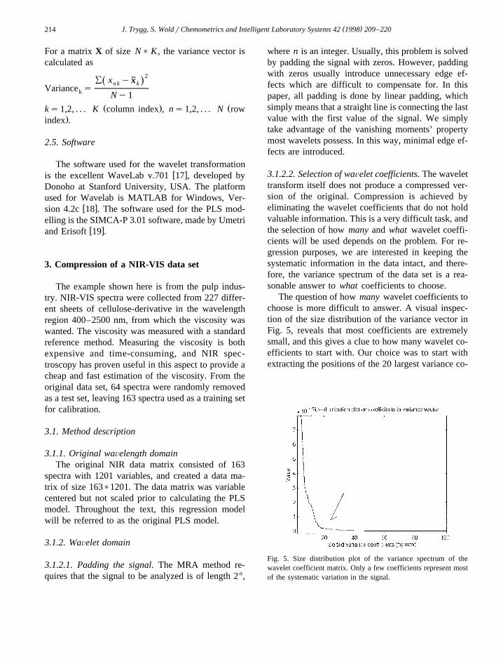
The question of how many wavelet coefficients tochoose is more difficult to answer. A visual inspec-tion of the size distribution of the variance vector inFig. 5, reveals that most coefficients are extremelysmall, and this gives a clue to how many wavelet co-efficients to start with. Our choice was to start withextracting the positions of the 20 largest variance co-

Fig. 5. Size distribution plot of the variance spectrum of thewavelet coefficient matrix. Only a few coefficients represent mostof the systematic variation in the signal.


efficients, and continue from there. It must be clearthat there is no guarantee that 20 coefficients areenough. It is necessary to look for the systematicchange in the data by adding more coefficients andcalculating additional PLS models. The optimal com-pression has most likely been achieved when the PLSmodels are similar.

3.1.2.3. Reconstruction. Wavelet transform is a lin-ear transform, and a complete reconstruction can bemade with all the calculated wavelet coefficients.However, using an orthogonal set of basis functions,which means that each wavelet function is indepen-dent of all the other ones, we can still reconstruct thesignal even if we have discarded some coefficients.This is very useful in our case. It is possible to re-construct the compressed spectra into the originaldomain, and also to reconstruct the original loadingspectrum for each component in the data compressedPLS model. When reconstructing the signal, the cho-sen wavelet coefficients are put back in their originalposition in the transformed vector, setting all othercoefficients to zero, and performing an inverse

Ž .wavelet transformation Fig. 6 .

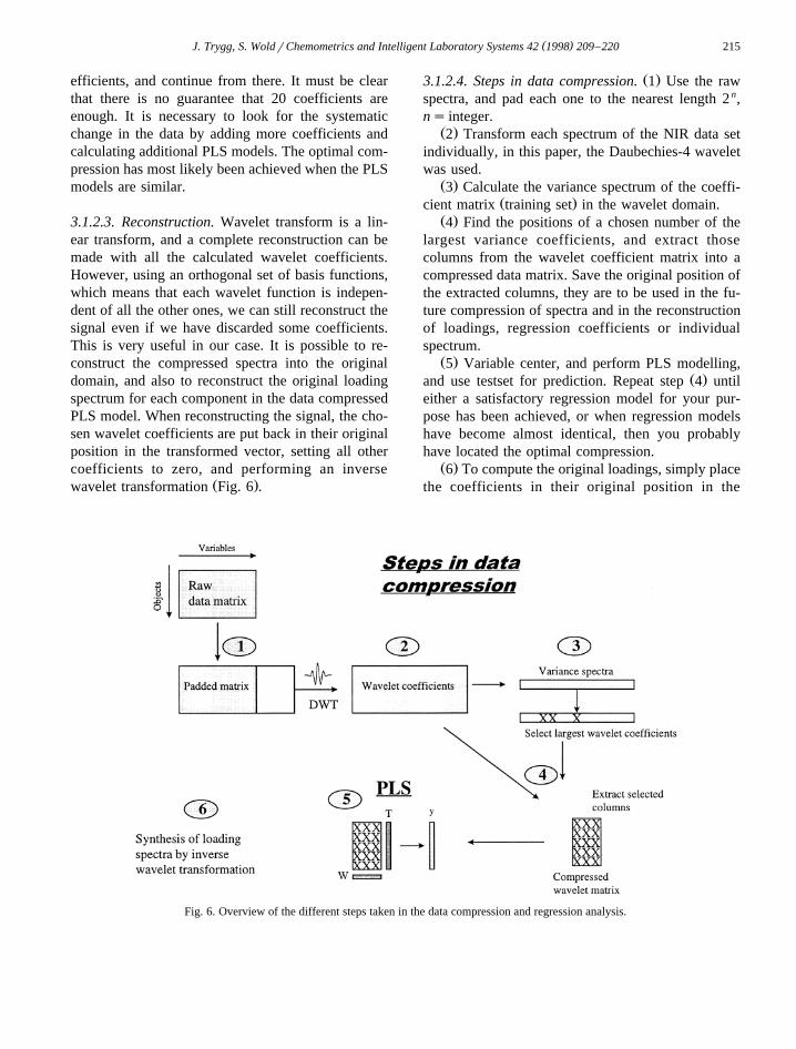
Ž .3.1.2.4. Steps in data compression. 1 Use the rawspectra, and pad each one to the nearest length 2 n,ns integer.

Ž .2 Transform each spectrum of the NIR data setindividually, in this paper, the Daubechies-4 waveletwas used.

Ž .3 Calculate the variance spectrum of the coeffi-Ž .cient matrix training set in the wavelet domain.

Ž .4 Find the positions of a chosen number of thelargest variance coefficients, and extract thosecolumns from the wavelet coefficient matrix into acompressed data matrix. Save the original position ofthe extracted columns, they are to be used in the fu-ture compression of spectra and in the reconstructionof loadings, regression coefficients or individualspectrum.

Ž .5 Variable center, and perform PLS modelling,Ž .and use testset for prediction. Repeat step 4 until

either a satisfactory regression model for your pur-pose has been achieved, or when regression modelshave become almost identical, then you probablyhave located the optimal compression.

Ž .6 To compute the original loadings, simply placethe coefficients in their original position in the

Fig. 6. Overview of the different steps taken in the data compression and regression analysis.


wavelet vector, fill all other positions with zeros, andperform inverse wavelet transformation.

4. Results

The results discussed here will focus on the com-parison between the original PLS model and the datacompressed PLS model.

Applying the wavelet transform as a preprocess-ing method shows promising compression results onnear-infrared spectra. Our choice of padding the sig-nal works, and produces small edge effects. Using thevariance vector from the wavelet coefficient matrix asa starting point in the selection of wavelet coeffi-cients is a good choice. All PLS models have beenvariable centered, and all components included have

w xbeen considered significant by cross-validation 20 .

4.1. Prediction ability

Results from the original PLS model with 1201variables are displayed in Table 1. The best regres-sion model gave 12 PLS components and predictedviscosity with a RMSEPs95 on the test set. Also inTable 1 are the modelling results from the data com-pressed PLS models, using different numbers ofwavelet coefficients. The compressed regressionmodels show similar results compared to the original

Table 1Modelling results for the original PLS model, and for the datacompressed PLS models

The original PLS model

Ž . Ž .No. of variables Total comp. R2 Y Q2 Y RMSEP

1201 12 0.97 0.94 96

The data compressed PLS models

20 12 0.951 0.927 11240 12 0.963 0.942 9960 12 0.964 0.945 9980 12 0.964 0.946 98

100 12 0.964 0.947 98150 12 0.965 0.948 97200 12 0.966 0.948 96

Results from using different numbers of wavelet coefficients aredisplayed. The chosen data compressed PLS model with 40 waveletcoefficients is shown in bold text.

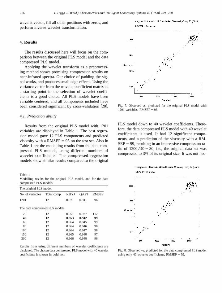
Fig. 7. Observed vs. predicted for the original PLS model with1201 variables, RMSEPs96.

PLS model down to 40 wavelet coefficients. There-fore, the data compressed PLS model with 40 waveletcoefficients is used. It had 12 significant compo-nents, and a prediction of the viscosity with a RM-SEPs99, resulting in an impressive compression ra-tio of 1200r40s30, i.e., the original data set wascompressed to 3% of its original size. It was not nec-

Fig. 8. Observed vs. predicted for the data compressed PLS modelusing only 40 wavelet coefficients, RMSEPs99.


essary to calculate data compressed PLS models withmore than 100 wavelet coefficients, but they werealso computed to show the stability of the PLS model.

The observed vs. predicted plots of the testset forboth the original PLS model and the data com-pressed PLS model with 40 wavelet coefficients, aredisplayed in Figs. 7 and 8. The results are very simi-lar between the original PLS model and the datacompressed PLS model, but remember that thewavelet compressed model has a 30 times smallerdata matrix.

4.2. Model diagnostics

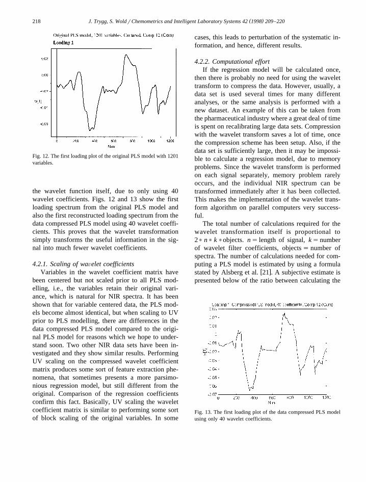
The diagnostics and the graphical displays from aregression model are also very important in order tobe able to understand and interpret the chemical in-formation in the model. All score plots and loadingplots look almost the same as the original PLS model.Figs. 9 and 10 show the similarity between the scoreplots.

A very nice property of the wavelet transforma-tion is the fact that it is possible to reconstruct notonly the NIR spectra themselves, but also individual

Fig. 9. Shows the t1– t2 score plot for the original PLS model with1201 variables.

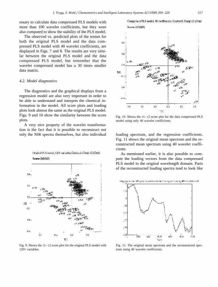
Fig. 10. Shows the t1– t2 score plot for the data compressed PLSmodel using only 40 wavelet coefficients.

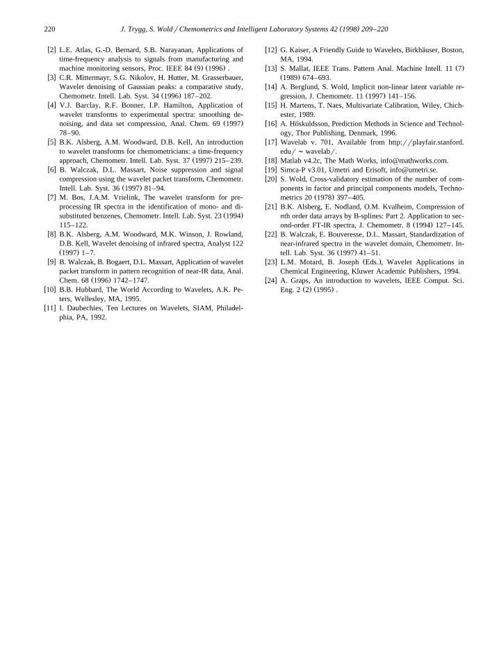
loading spectrum, and the regression coefficients.Fig. 11 shows the original mean spectrum and the re-constructed mean spectrum using 40 wavelet coeffi-cients.

As mentioned earlier, it is also possible to com-pute the loading vectors from the data compressedPLS model to the original wavelength domain. Partsof the reconstructed loading spectra tend to look like

Fig. 11. The original mean spectrum and the reconstructed spec-trum using 40 wavelet coefficients.


Fig. 12. The first loading plot of the original PLS model with 1201variables.

the wavelet function itself, due to only using 40wavelet coefficients. Figs. 12 and 13 show the firstloading spectrum from the original PLS model andalso the first reconstructed loading spectrum from thedata compressed PLS model using 40 wavelet coeffi-cients. This proves that the wavelet transformationsimply transforms the useful information in the sig-nal into much fewer wavelet coefficients.

4.2.1. Scaling of waÕelet coefficientsVariables in the wavelet coefficient matrix have

been centered but not scaled prior to all PLS mod-elling, i.e., the variables retain their original vari-ance, which is natural for NIR spectra. It has beenshown that for variable centered data, the PLS mod-els become almost identical, but when scaling to UVprior to PLS modelling, there are differences in thedata compressed PLS model compared to the origi-nal PLS model for reasons which we hope to under-stand soon. Two other NIR data sets have been in-vestigated and they show similar results. PerformingUV scaling on the compressed wavelet coefficientmatrix produces some sort of feature extraction phe-nomena, that sometimes presents a more parsimo-nious regression model, but still different from theoriginal. Comparison of the regression coefficientsconfirm this fact. Basically, UV scaling the waveletcoefficient matrix is similar to performing some sortof block scaling of the original variables. In some

cases, this leads to perturbation of the systematic in-formation, and hence, different results.

4.2.2. Computational effortIf the regression model will be calculated once,

then there is probably no need for using the wavelettransform to compress the data. However, usually, adata set is used several times for many differentanalyses, or the same analysis is performed with anew dataset. An example of this can be taken fromthe pharmaceutical industry where a great deal of timeis spent on recalibrating large data sets. Compressionwith the wavelet transform saves a lot of time, oncethe compression scheme has been setup. Also, if thedata set is sufficiently large, then it may be impossi-ble to calculate a regression model, due to memoryproblems. Since the wavelet transform is performedon each signal separately, memory problem rarelyoccurs, and the individual NIR spectrum can betransformed immediately after it has been collected.This makes the implementation of the wavelet trans-form algorithm on parallel computers very success-ful.

The total number of calculations required for thewavelet transformation itself is proportional to2) n) k)objects. ns length of signal, ksnumberof wavelet filter coefficients, objects s number ofspectra. The number of calculations needed for com-puting a PLS model is estimated by using a formula

w xstated by Alsberg et al. 21 . A subjective estimate ispresented below of the ratio between calculating the

Fig. 13. The first loading plot of the data compressed PLS modelusing only 40 wavelet coefficients.


data compressed PLS model and the original PLSmodel for the NIR example of 227 spectra includingthe testset.

CompressionqPLSŽ .s0.23

PLS originalŽ .

This ratio would be much less if we would haveused the iterative PCA instead or even PLS with sev-eral y-variables, since PLS with one y-variable iter-ates only once. Also, the wavelet transform is per-formed only once, which means that computing a fewdata compressed PLS models does not change theabove estimated ratio to any extent.

5. Conclusion

The wavelet transformation is a very powerfulmethod for compressing data. It works similar toholograms, which can capture a picture in a few pix-els without distorting it. This report has been a firstinvestigation on how the wavelet transform can beused as an effective compression preprocessing tech-nique in multivariate calibration. Of course, any mul-tivariate method may be employed, PCA, PCR, NN,to name a few. We have only used the popularDaubechies-4 wavelet. We could have used manyother types of wavelets, but the Daubechies wavelethas nice properties and is fast to calculate. Also, theuse of other wavelet functions have shown similarresults as reported here. This indicates that for NIRspectra compression, it is not worth optimizing whatwavelet basis to use, a simple wavelet like theDaubechies-4 works satisfactory.

The discrete wavelet transformation is easy to un-derstand and to implement on computers and will re-duce the computational time needed significantlyonce a compression scheme has been setup. Since thewavelet transform is calculated on each spectrum in-dividually, implementations on parallel computers arevery successful. Our NIR example showed that in-stead of using 1201 variables, the same regressionmodel was produced using only 40 wavelet coeffi-cients, reducing the size of the data set to 3% of itsoriginal size. Reconstructing the loading spectra inthe wavelet domain into the original wavelength do-main is straightforward. The results are almost iden-

tical compared to the loading spectra of the originalPLS model.

In regression analysis, the variance spectrum in thewavelet domain should be a good choice for the se-lection of wavelet coefficients. It is a difficult task tochoose the correct number of coefficients for opti-mum compression, but a good starting estimate canbe achieved by a visual inspection of the size distri-bution of the variance vector, and then a few addi-tional coefficients are added until the PLS model sta-bilizes.

The wavelet transform is of course not unique forNIR spectra. Originally, wavelets were created tobetter represent complicated signal that were sharpand non-stationary. In the near future, we will inves-tigate how the wavelet transform can be used to-gether with other preprocessing techniques, such ascalibration transfer and scatter correction. Initial at-tempts to use the wavelet transform in calibration

w xtransfer has been done by Walczak et al. 22 .The wavelet transform will certainly prove worthy

to many applications not yet found. Knock detectionin engines, diagnosing Alzheimer’s disease fromEEG, discovering underground oil, compression offingerprints, to name a few areas where it has beensuccessful, and it will keep on being successful, butit will not perform miracles.

Acknowledgements

The authors would like to thank Chris Stork,CPAC, Center for Process Analytical Chemistry,University of Washington, Seattle, USA, for givingan introduction to the wavelet transform. Manythanks also to Henrik Antti, University of Umea, for˚providing the NIR data set. Support from the Swedish

Ž .Natural Science Research Council NFR NationalŽ .Graduate School in Scientific Computing NGSSC ,

and Skogsbio-teknik och kemi, is gratefully ac-knowledged.

References

w x1 L.R. Dragonette, D.M. Drumheller, C.F. Gaumond, D.H.Hughes, B.T. O’Connor, N.C. Yen, The application of two-dimensional signal transformations to the analysis and syn-thesis of structural excitations observed in acoustical scatter-

Ž . Ž .ing, Proc. IEEE 84 9 1996 .


w x2 L.E. Atlas, G.-D. Bernard, S.B. Narayanan, Applications oftime-frequency analysis to signals from manufacturing and

Ž . Ž .machine monitoring sensors, Proc. IEEE 84 9 1996 .w x3 C.R. Mittermayr, S.G. Nikolov, H. Hutter, M. Grasserbauer,

Wavelet denoising of Gaussian peaks: a comparative study,Ž .Chemometr. Intell. Lab. Syst. 34 1996 187–202.

w x4 V.J. Barclay, R.F. Bonner, I.P. Hamilton, Application ofwavelet transforms to experimental spectra: smoothing de-

Ž .noising, and data set compression, Anal. Chem. 69 199778–90.

w x5 B.K. Alsberg, A.M. Woodward, D.B. Kell, An introductionto wavelet transforms for chemometricians: a time-frequency

Ž .approach, Chemometr. Intell. Lab. Syst. 37 1997 215–239.w x6 B. Walczak, D.L. Massart, Noise suppression and signal

compression using the wavelet packet transform, Chemometr.Ž .Intell. Lab. Syst. 36 1997 81–94.

w x7 M. Bos, J.A.M. Vrielink, The wavelet transform for pre-processing IR spectra in the identification of mono- and di-

Ž .substituted benzenes, Chemometr. Intell. Lab. Syst. 23 1994115–122.

w x8 B.K. Alsberg, A.M. Woodward, M.K. Winson, J. Rowland,D.B. Kell, Wavelet denoising of infrared spectra, Analyst 122Ž .1997 1–7.

w x9 B. Walczak, B. Bogaert, D.L. Massart, Application of waveletpacket transform in pattern recognition of near-IR data, Anal.

Ž .Chem. 68 1996 1742–1747.w x10 B.B. Hubbard, The World According to Wavelets, A.K. Pe-

ters, Wellesley, MA, 1995.w x11 I. Daubechies, Ten Lectures on Wavelets, SIAM, Philadel-

phia, PA, 1992.

w x12 G. Kaiser, A Friendly Guide to Wavelets, Birkhauser, Boston,¨MA, 1994.

w x Ž .13 S. Mallat, IEEE Trans. Pattern Anal. Machine Intell. 11 7Ž .1989 674–693.

w x14 A. Berglund, S. Wold, Implicit non-linear latent variable re-Ž .gression, J. Chemometr. 11 1997 141–156.

w x15 H. Martens, T. Naes, Multivariate Calibration, Wiley, Chich-ester, 1989.

w x16 A. Hoskuldsson, Prediction Methods in Science and Technol-¨ogy, Thor Publishing, Denmark, 1996.

w x17 Wavelab v. 701, Available from http:rrplayfair.stanford.edur ; wavelabr.

w x18 Matlab v4.2c, The Math Works, [email protected] x19 Simca-P v3.01, Umetri and Erisoft, [email protected] x20 S. Wold, Cross-validatory estimation of the number of com-

ponents in factor and principal components models, Techno-Ž .metrics 20 1978 397–405.

w x21 B.K. Alsberg, E. Nodland, O.M. Kvalheim, Compression ofnth order data arrays by B-splines: Part 2. Application to sec-

Ž .ond-order FT-IR spectra, J. Chemometr. 8 1994 127–145.w x22 B. Walczak, E. Bouveresse, D.L. Massart, Standardization of

near-infrared spectra in the wavelet domain, Chemometr. In-Ž .tell. Lab. Syst. 36 1997 41–51.

w x Ž .23 L.M. Motard, B. Joseph Eds. , Wavelet Applications inChemical Engineering, Kluwer Academic Publishers, 1994.

w x24 A. Graps, An introduction to wavelets, IEEE Comput. Sci.Ž . Ž .Eng. 2 2 1995 .

PLS regression on wavelet compressed NIR spectra

Documents