Plotting II: By the end of this class you should be able to: Create a properly formatted engineering graph Create graphs of a function Place multiple plots.

Plotting II:By the end of this class you should be able

to:

• Create a properly formatted engineering graph• Create graphs of a function • Place multiple plots in one figure• Plot a polynomial functions• Find polynomial roots by graph and by

command• Change the tick marks and tick labels on a

graph

Text: §§ 5.1 - 5.3

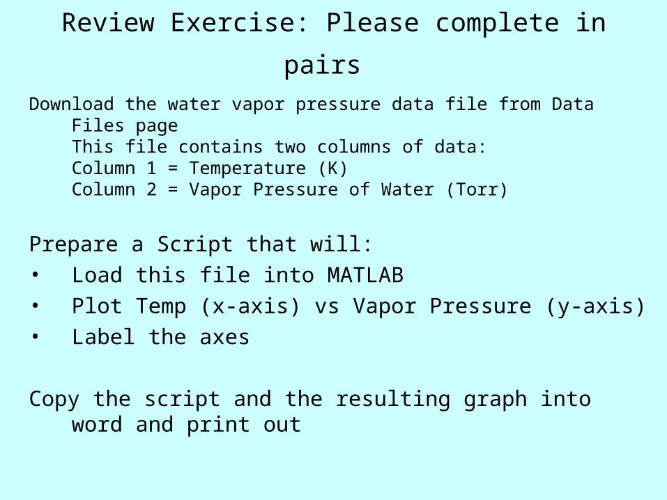
Review Exercise: Please complete in pairs

Download the water vapor pressure data file from Data Files pageThis file contains two columns of data:

Column 1 = Temperature (K)Column 2 = Vapor Pressure of Water (Torr)

Prepare a Script that will:• Load this file into MATLAB• Plot Temp (x-axis) vs Vapor Pressure (y-axis)• Label the axes

Copy the script and the resulting graph into word and print out

Graphing Requirements

( pg 262)

300 400 500 600 700 800 900 10000

2

4

6

8

10

12

14

16

18

20

RCX Raw Value

He

igh

t (cm

)

Level Calibration - data from LegoLevel.mat

Group 1 dataFit: ht=29-0.028*raw

1. axis

label with quantity and units

2. regularly

spaced, easy to interpret tick marks

3. label

multiple curves

4. use title to distinguish

as necessary

5. plot data using a symbol

(6. avoid connection lines)

7. Plot

functions using lines

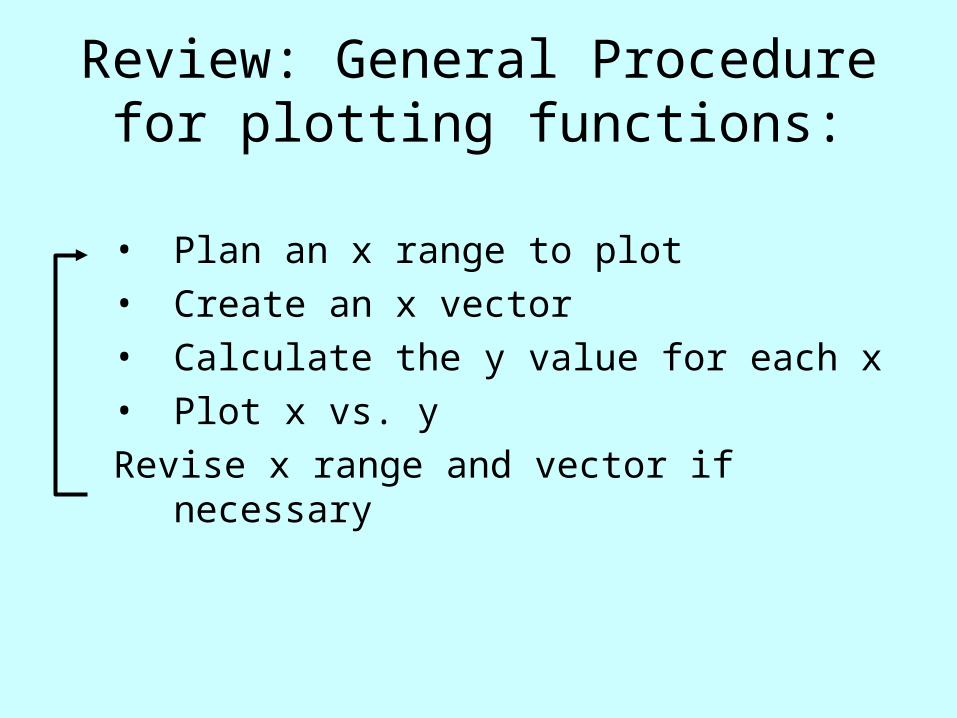
• Plan an x range to plot• Create an x vector • Calculate the y value for each x • Plot x vs. y Revise x range and vector if

necessary

Review: General Procedure for plotting functions:

A projectile is thrown straight upward.It’s height is governed by the formula:

where: h = height of the projectile

v0 = the initial velocity of the projectile

= 50 m/st = the elapsed time in secondsg = the acceleration of gravity = 9.8 m/s2

How would you plot the height of the projectile vs. time?

20 2

1gttvh

Write a function to plot height of projectile vs. time (complete a function development worksheet in the

process)

It’s height is governed by the formula:

where: h = height of the projectile

v0 = the initial velocity of the projectile

= 50 m/st = the elapsed time in secondsg = the acceleration of gravity = 9.8 m/s2

Also Remember:

20 2

1gttvh

g

vtend

02

Graphing Hints( pg 281, 282)

300 400 500 600 700 800 900 10000

2

4

6

8

10

12

14

16

18

20

RCX Raw Value

He

igh

t (cm

)

Level Calibration - data from LegoLevel.mat

Group 1 dataFit: ht=29-0.028*raw

Plan AxesUse sensible

tick mark spacing

Avoid trailing zeros

Start Axes from zero whenever possible

Use different line types for each curve

(plots must be “xeroxible” )

Use same axis range and tick mark spacing for graphs that

will be compared

Avoid clutter (too many

curves in one area)

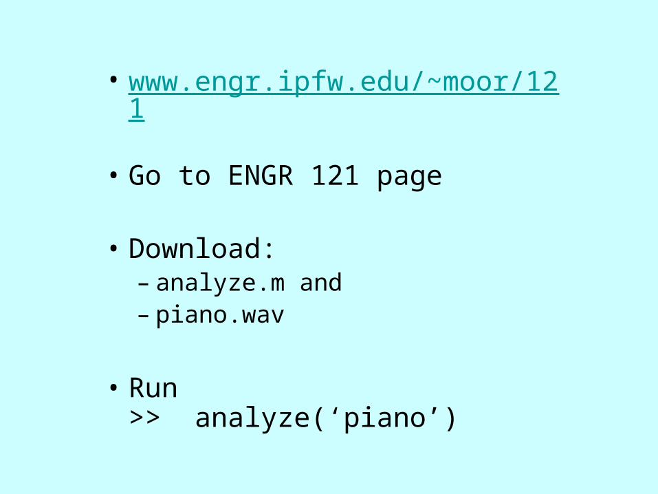
• www.engr.ipfw.edu/~moor/121 • Go to ENGR 121 page

• Download: – analyze.m and – piano.wav

• Run >> analyze(‘piano’)

0.105 0.11 0.115

-0.8

-0.6

-0.4

-0.2

0

0.2

0.4

0.6

Waveform of piano

0 1000 2000 3000 400010

-4

10-3

10-2

10-1

100

Power Spectrum of piano

Analyze.m[y, Fs] = wavread(file); % y is sound data, Fs is sample frequency.t = (1:length(y))/Fs; % time

ind = find(t>0.1 & t<0.12); % set time duration for waveform plotfigure; subplot(1,2,1)plot(t(ind),y(ind)) axis tight title(['Waveform of ' file])

N = 2^12; % number of points to analyzec = fft(y(1:N))/N; % compute fft of sound datap = 2*abs( c(2:N/2)); % compute power at each frequencyf = (1:N/2-1)*Fs/N; % frequency corresponding to p

subplot(1,2,2)semilogy(f,p)axis([0 4000 10^-4 1]) title(['Power Spectrum of ' file])