Plausibility test of conceptual soil maps using relief parameters

(This is a sample cover image for this issue. The actual cover is not yet available at this time.)

This article appeared in a journal published by Elsevier. The attachedcopy is furnished to the author for internal non-commercial researchand education use, including for instruction at the authors institution

and sharing with colleagues.

Other uses, including reproduction and distribution, or selling orlicensing copies, or posting to personal, institutional or third party

websites are prohibited.

In most cases authors are permitted to post their version of thearticle (e.g. in Word or Tex form) to their personal website orinstitutional repository. Authors requiring further information

regarding Elsevier’s archiving and manuscript policies areencouraged to visit:

http://www.elsevier.com/copyright

http://www.elsevier.com/copyright

Author's personal copy

Plausibility test of conceptual soil maps using relief parameters

Markus Möller a,⁎, Thomas Koschitzki b, Klaus-Jörg Hartmann c, Reinhold Jahn d

a University Halle-Wittenberg, Department of Remote Sensing and Cartography, Von-Seckendorff-Platz 4, 06120 Halle (Saale), Germanyb Geoflux GbR, Lessingstr. 37, 06114 Halle (Saale), Germanyc State Institute for Geology and Natural Resources Saxony-Anhalt, Köthener Str. 38, 06118 Halle (Saale), Germanyd University Halle-Wittenberg, Department of Soil Science and Soil Conservation, Von-Seckendorff-Platz 3, 06120 Halle (Saale), Germany

a b s t r a c ta r t i c l e i n f o

Article history:Received 24 August 2010Received in revised form 18 July 2011Accepted 19 August 2011Available online xxxx

Keywords:Digital soil mappingTerrain analysisSegmentationExpert knowledgeCluster analysisKolmogorov Smirnov test

The motivation for this article results from the fact that conceptual soil maps show oftentimes inaccuracieswith regard to soil unit boundaries or misfits between original paper and actual soil-related information.Using the example of a German conceptual soil map (CSM), we introduce a procedure which could be con-sidered as a framework for testing the terrain-related plausibility applied within a genetic based soil-orderingsystem. Framework means that all tests and the underlying methods can be adapted to specific targets. Theprocedure enables both reproducible integration of expert knowledge and application of statistically soundmethods.The CSM of the German Federal State of Saxony-Anhalt was tested regarding the plausibility of colluvialand fluvial process domains. The plausibility test consists of four steps and was exemplified on a studyarea of 100 km2. First, basic relief parameters were combined to the explaining relief parameters FloodplainIndex (FPI) andMass Balance Index (MBI) enabling a classification of process domains by relative descriptions.Second, relief parameters and aggregated CSM soil units were integrated to soil-terrain objects (STO) execut-ing a region-growing segmentation algorithm. In the third step, the one-dimensionalMBI or FPI feature spaceof STO entities were clustered by using the K-means algorithm. The fourth step comprises the expert-basedselection of reference clusters (RC) representing colluvial and fluvial process domains accepted as being true.Then, empirical cumulative distribution functions (ECDF) of RC and remaining soil unit-related STO clusterswere compared by a traditional goodness-of-fit test whose suitability for estimation of terrain-related CSMplausibility is shown. Finally, the resulting ECDF distances were visualized.The testing procedure could also be used for the supervised selection of appropriate samples for automaticclassification algorithms. The data integration approach is generally suitable for adopting existing data incomputer-based systems.

© 2011 Elsevier B.V. All rights reserved.

1. Introduction

Conceptual soil maps (CSM) are the result of an expert-based inte-gration process wherein different soil-related information or alreadyexisting older soil maps are combined by soil surveyors (Dobos andHengl, 2009). The resulting soil maps “are representations of struc-tured knowledge” (Bui, 2004). The data integration process is mainlyguided by the ordering system. Genetic soil-ordering concepts arebased on generally accepted perceptions of soil genesis and allowmore expert-based interpretation than classification systems wherethreshold defined diagnostic horizons, features and the horizon se-quences determine soil units (Albrecht et al., 2005; Buol et al., 2003).

A German CSM example is the preliminary soil map 1:50,000 ofSaxony-Anhalt (in German: “Vorläufige Bodenkarte 1:50,000” orVBK 50; Hartmann, 2005, 2006). The VBK 50 map results from an

expert-based integration process where older soil maps were semanti-cally transferred into the actual (genetic) German soil ordering system(Ad-hoc AG, 2005). The soil map contains typical CSM inaccuracies.First, misfits between original paper and actual, more accurate soil-related information exist. Second, locations of systematic soil unitboundaries are often incorrect due to their subjective delineation.This can be observed especially between areas of fluvial and terres-trial process domains. A special problem is related to the attributestructure of the used older soil maps which were the basis of theCSM creation (Deumlich et al., 1998; Müller and Volk, 2001). The at-tributes describe heterogeneous soil units of genetically linked soils.That means that the occurrence of some – especially colluvial – soilunits are only listed in the attribute table but not represent polygons(Möller, 2008).

The mentioned inaccuracies are mostly terrain-related and concernespecially colluvial and fluvial process domains. Information about sur-face topography can nowadays be derived from easily accessible digitalelevation models (DEM) in different spatial resolutions and accuracies(Hengl and MacMillan, 2009). Thus, the main objective of this study is

Catena 88 (2012) 57–67

⁎ Corresponding author. Tel.: +49 345 5526025; fax: +49 345 2394019.E-mail address: [email protected] (M. Möller).URL: http://www.geo.uni-halle.de/geofern/mitglieder/moeller/ (M. Möller).

0341-8162/$ – see front matter © 2011 Elsevier B.V. All rights reserved.doi:10.1016/j.catena.2011.08.002

Contents lists available at SciVerse ScienceDirect

Catena

j ourna l homepage: www.e lsev ie r .com/ locate /catena


the development and application of a procedure testing the colluvialand fluvial plausibility of VBK 50. Furthermore, heterogeneous soilunits should be geometrically disaggregated regarding the occurrenceof colluvial process domains.

In this study, the plausibility test is demonstrated on the exampleof the German topographic map TK25 4336 Könnern at a scale of1:25,000 with an area of about 100 km2. In a joint project of astate authority, a scientific institution and an engineering office, theprocedure was applied on the total area of the German Federal Stateof Saxony-Anhalt (≈20,000 km2). The project's outcome can be con-sidered as a compromise solution, in which pedological and digitalsoil mapping (DSM) expertise were balanced.

We are using the term plausibility instead of quality or accuracy.Quality and accuracy are related to international standards for geo-data (e.g. ISO 19138, 2006). This should help data producers objec-tively describe the quality of data and determine its quality usingstatistical calculation rather than subjective estimation. Althoughwe support the utilization of statistical quality measures, we also rec-ognize the need for possibilities to deal with expert knowledge in areproducible manner (see Deumlich et al., 2010). The integrating re-sult of subjective and objective quality to assess the soil map's good-ness we refer to as plausibility.

In this study, plausibility is considered as distance between refer-ence and test distributions of explaining relief parameters. We showhow basic relief parameters can be combined to specific indices whichexplain the occurrence of colluvial and fluvial process domains. Further-more, we demonstrate how reference distributions can be defined byexpert-knowledge in a transparent and traceable manner. Finally, thesuitability of a traditional goodness-of-fit-test for comparing relief pa-rameters' distributions is investigated.

2. Materials and methods

2.1. Study site

The study area is situated in the German Federal State of Saxony-Anhalt and represents heterogeneous soil and relief conditions (Fig. 1,Table 1; Möller et al., 2008). The formation of parent materials, reliefand soil formation was connected with glacial and periglacial con-ditions during the Saalian and Weichselian glacial stages where pla-teaus and floodplains were shaped. Plateaus and plateau margins aremainly covered by Weichselian loess and Saalian moraine materi-al. There, calcareous Ah/C and black soils dominate (Pararendzina,Tschernosem). Where older sandstones, clay or limestones of mainly

Fig. 1. Study site location as well as its soil (see Table 1) and terrain conditions (Data sources: Soil units — http://www.lagb.sachsen-anhalt.de | DEM — http://www.lvermgeo.sachsen-anhalt.de).

58 M. Möller et al. / Catena 88 (2012) 57–67


Permian and Carboniferous ages emerge, brown soils and Ah/C soilfrom silicatic rock occur (Braunerde and Ranker). Floodplain andgroundwater affected soils have developed in the fluvial sediments(Vega, Tschernitza, Kalkpaternia, Gley). The occurrence of colluvial soils(Kolluvisol) is favored by the intensive agriculture and intense summerrainstorm events.

2.2. Workflow

The procedure consists of four steps (Fig. 2). On the basis of a dig-ital elevation model (DEM), the starting point of the workflow is the

derivation of appropriate relief parameters (Section 2.2.1). Our basicapproach is to combine several basic relief parameters (DEMRP) toas few as possible combined relief parameters on demand (DEMCP).The parameter combination is guided by the objective of the test. Inthis study, colluvial and fluvial process domains should be character-ized. The combination is carried out in such a way that process do-mains can be classified by relative descriptions. Relative definitionslike minimum or maximum values enable an easier integration of ex-pert knowledge. In addition, classification models can be better trans-ferred to other geomorphologic regions (Dragut and Blaschke, 2006;Möller et al., 2008).

The data integration procedure in the second step of the workflowaims at the coupling of the CSM data set and the predicting relief pa-rameters (DEMCP). For this purpose, the CSM spatial domains weresubdivided into soil-terrain objects (STO) by the application of a seg-mentation algorithm (Section 2.2.2). STOs can be characterized asgroups of pixels of different relief parameters which are aggregatedto landform elements according to a scale-specific homogeneity(Dragut and Eisank, 2011; MacMillan and Shary, 2009; Minár andEvans, 2008) considering already existing soil map boundaries. Instep 3, two STO groups have to be defined:

1. STOP are segmented systematical soil units which should be testedregarding their terrain-related plausibility. In this study, soil unitswere aggregated according to their dominating soil-terrain-related formation (Table 2). The areas of aggregated soil units areshown in Fig. 5a. Accordingly, the aggregated soil units T and R/Bdominate spatially while the units A/G and especially Y are repre-sented by smaller areas.

2. STOR stands for a segmented soil unit which represents the processdomain of interest provided by the original CSM. In Table 2, the as-sociated (here: colluvial and fluvial) CSM soil units are gray em-phasized. While the soil unit YK is affected by colluvial processes,the soil units GG, AB, AT, AZ, GG-AT are mainly influenced by fluvi-al processes. In the following, both groups are classed as Y and A/G.STOA/G and STOY are the basis for the selection of reference clusters(RC).

The clustering procedure can be considered as statistical groupingof a feature space (Section 2.2.3). The grouping refers to the specificDEMCP feature space of STO entities. Each STO entity covers an aggre-gated soil unit and is separately clustered. According to Table 2, fourentities are to be clustered in this study (STOY, STOA/G, STOT,STOR/B). The grouping leads to STOR and STOP clusters which are la-beled as Ri and Pi. Reference clusters (RC) are determined by experts.This crucial operation is supported by the specific DEMCA propertieswhich enable a relative classification (see step 1). The considerationof Ri cluster values, their visualization in feature space and as seg-mented and clustered soil map helps to identify RCs. In other words,RC are STOR (here: STOY or STOA/G) with a representative value distri-bution of the (here: colluvial or fluvial) process domain of interestwhich is accepted as being true.

Fig. 2. Workflow. DEM — digital elevation model | DEMRP — basic relief parameter |DEMCP — combined relief parameter on demand | CSM — conceptual soil map | STO— soil-terrain object | STOP — STOs which should be tested | STOR — STOs representingthe process domain of interest based on CSM | RC — STOR clusters representingterrain-related process domains of interest selected by experts | Ri — STOR clusters |Pi — STOP clusters | Ci — Ri which are confirmed regarding terrain-related processdomains | Ni — Ri which are rejected regarding terrain-related process domainsand have to be newly classified | RPi – STOP clusters which are tested positive re-garding terrain-related process domains.

Table 2Aggregation criteria for soil units. The gray emphasized soil units represent fluvial (A/G)and colluvial process domains of interest (Y).

Aggregated

soil unit

Soil unit Aggregation criterion

A/G GG, AB, AT, AZ, GG-AT* Dominating fluvial processes

R/B BB, RN, RZ Dominating processes of solifluc-

tion, humus layer thickness < 4 dm

T BB-TT, GG-TT, SS-TT,

TT

Dominating processes of solifluc-

tion, humus layer thickness > 4 dm

Y YK Dominating processes of solifluction

and colluvial process domains

⁎ In fact, GG stands for soils with gleyic properties (Gleysols). However, all Gleysolsof the study area are situated within floodplains. Thus, these soils are also characterized byfluvial properties.

Table 1German systematical soil units according to Ad-hoc AG (2005) and the most probablereference soil groups according to IUSS Working Group (2006).

German soilunit

Short description Most probable reference soil group

RN Ranker Ah/C soils fromsilicatic rock

Haplic Leptosol from periglacial layersof sandstone

RZ Pararendzina Calcareous Ah/Csoils

Haplic Regosol Calcaric from periglaciallayers of loess or marly materials

TT Tschernosem Black soils Haplic Chernozem from loessBB Braunerde Brown soils Haplic Cambisol from periglacial layers

of sandstoneYK Kolluvisol Soils from eroded

top soil materialColluvic Regosol from colluvic loessmaterial

AB Vega Brown floodplainsoils

Endofluvic Cambisol from fluvicmaterial

AT Tschernitza Chernozem likefloodplain soils

Endofluvic Chernozem from fluvicmaterial

AT Kalkpaternia Calcareous Ah/Cfloodplain soils

Haplic Fluvisol from fluvic material

GG Gley Groundwateraffected soils

Endofluvic Endogleyic Cambisol fromfluvic material

59M. Möller et al. / Catena 88 (2012) 57–67


Step 4 of the procedure comprises the comparison of RC and Pi dis-tributions by the application of a goodness-of-fit test (Section 2.2.4).As a result, four types of clusters emerge:

1. STOR clusters which are confirmed (Ci),2. STOR clusters which are rejected and have to be newly classified

(Ni),3. STOP clusters which are statistically similar to RC (RPi) and4. STOP clusters which are not similar to RC (Pi).

2.2.1. Digital elevation model and calculation of relief parametersThe used state-wide available digital elevation model (DEM) was

originally generated by the digitalization of elevation contours of to-pographic maps in a scale of 1:10,000. The ANUDEM algorithm byHutchinson (1989) was applied in order to create a hydrologicalsound DEM with a resolution of 20 m (see Fig. 1).

The calculation of basic relief parameters was performed withinSAGA GIS and RSAGA environment using the application rsaga.geoprocessor1 (Brenning, 2008; Olaya and Conrad, 2009). Slope (S)and Total Curvature (TC) are standard relief parameters and were calcu-lated according to Zevenbergen and Thorne (1987). The parameterVertical Distance to Channel Network (VDN) is the difference betweenthe original elevation DEM and the interpolated channel network base

level (DEMBASE,N; Eq. (1)). The calculation of the parameters Vertical Dis-tanceto River Network (VDR) and Vertical Distance to Culmination Net-work (VDC) is similar to Eq. (1) however the reference for the baselevel interpolation differs. VDR uses the river network as reference(DEMBASE,R, Eq. (2)). The comparison of Fig. 3a and b reveals the dif-ference between river and channel network. VDC is referring to theculmination network resulting from a reversed DEM (DEMr). Here,the base level is named as DEMr,BASE,C (Eq. (3)).

VDN ¼ DEM−DEMBASE;N ð1Þ

VDR ¼ DEM−DEMBASE;R ð2Þ

VDC ¼ DEMr−DEMr;BASE;C ð3Þ

In addition, the well-known Topographic Wetness Index (TWI) wascalculated according to Eq. (4) where A is the Specific Catchment and Sthe Slope (Quinn et al., 1995).

TWI ¼ lnA

tan Sð Þ� �

ð4Þ

All relief parameters were transformed into a unique value rangeby the application of Eq. (5). x stands for the corresponding relief pa-rameter and F is a user-defined transfer constant affecting the1 http://cran.r-project.org/web/packages/RSAGA/RSAGA.pdf.

ID 1

ID 24

a) MBI, channel network (blue) and cross section 1 (red)

ID 1

ID 70

b) FPI, river network (blue) and cross section 2 (red)

5 10 15 20

142

146

150

154

Elevation

E [m

]

5 10 15 20

0.0

0.5

1.0

Mass balance index

Grid cell ID

MB

I

c) Cross section 1

0 10 20 30 40 50 60 70

100

140

ElevationE

[m]

0 10 20 30 40 50 60 70

0.0

0.5

1.0

1.5

2.0

Floodplain Index

Grid cell ID

FP

I

d) Cross section 2

Fig. 3. Relations between DEM cross sections and value ranges of MBI (a, c) and FPI (b, d).



parameter's value distribution (Friedrich, 1996; Friedrich, 1998).Here, F values of 15 (S, VDN, VDR, VDC, TWI) and 0.01 (TC) wereused leading to balanced ratio of dominating (e.g. floodplains) andsmaller landforms (e.g. depressions; Möller et al., 2008).

f xð Þ ¼ xxj j þ F

ð5Þ

with x=S, VDN, VDC, VDR, TWI, TC; f(S, VDN, VDC, VDR, TWI)∈ [0, 1];f(TC)∈ [−1, 1]

2.2.2. SegmentationIn this study, the region growing segmentation algorithm Fractal

Net Evolution Approach (FNEA) described in detail by Baatz andSchäpe (2000) was applied to relief parameters. The algorithm relieson seed pixel groups with both the smallest (here: Euclidean) dis-tance in pixel raster and in n-dimensional feature space of the usedrelief parameters. Then, the seeds grow as far as a halting criterionis fulfilled. The halting criterion could be a specific object heterogene-ity or existing boundaries. The segmentation process leads to differ-ent aggregation levels of discrete landform elements. Each levelrepresents a specific target scale consisting of objects with a compara-ble heterogeneity. The segmentation results can be influenced by pa-rameters which allow the adaptation of the target segment'sheterogeneity and shape (Möller et al., 2008).

FNEA has been proven as a suitable algorithm for detecting objectshaving meaning for soil-terrain-related issues (Dragut and Eisank,2011). A crucial point is the determination of an optimal segmenta-tion parameter setting (Dragut et al., 2009). Similar to Dragut andBlaschke (2006), we compared different segmentation results withsignificant known landforms like valleys and slope positions repre-senting minimal object sizes.

2.2.3. Cluster analysisClustering belongs to the standard techniques of unsupervised

learning and aims at the grouping of similar objects. In contrast tothe aforementioned FNE algorithm, similarity only refers to featurespace of data points (here: explaining relief parameters). The appliedK-means algorithm uses the squared Euclidean distance as dissimilar-ity measure. The algorithm is described in detail by Hastie et al.(2009). Starting with a user-defined number of initial K centroids,each data point is iteratively assigned to the nearest cluster centroid.The maximum number of iterations must be specified by the analyst.

2.2.4. Comparing distributionsThe comparison of reference clusters (RC) and clustered soil units

(Pi) is done by the Kolmogorov Smirnov goodness-of-fit (KS) test(Davis, 2002; Thas, 2010). The main advantage of this nonparametrictwo-sample test – especially in dealing with environmental data – isthe fact that any kind of distribution can be compared without requir-ing specific statistical conditions. Based on the empirical cumulativedistribution function (ECDF) the KS test verifies whether two distri-butions are the same (null hypothesis) or significantly differentfrom each other. The degree of difference is expressed by the maximalabsolute difference D between the cumulative distributions of RC andPi (Eq. (6)). Both K-means clustering and KS test were executed with-in the statistical environment R2 using the functions kmeans3 andks.test.4

D ¼ max ECDFRC−ECDFPij j ð6Þ

3. Results

3.1. Step 1: Combination of relief parameters on demand

TheMass Balance Index (MBI) was used to characterize colluvial soilprocess domains. NegativeMBI values represent areas of net depositionsuch as depressions and valleys, positiveMBI values indicate areas of neterosion such as convex hill slopes, MBI values close to 0 refer to areaswith a balance between erosion and deposition such as plain areas(Fig. 3a, c). MBI results from the combination of transformed relief pa-rameters f(S), f(VDN) and f(TC) (Eq. (7), see Section 2.2.1; Möller et al.,2008).

MBI ¼ f TCð Þ× 1−f Sð Þð Þ× 1−f VDNð Þð Þ for f TCð Þ b 0f TCð Þ× 1þ f Sð Þð Þ× 1þ f VDNð Þð Þ for f TCð Þ N 0

�ð7Þ

As the name implies, the Floodplain Index (FPI) enables the detec-tion of floodplains. Floodplains are located lower than their surround-ings which can be expressed by the relief parameter Relative SlopePosition (RSP). RSP is calculated according to Eq. (8) from the quotientof f(VDR) and the sum of f(VDR) and f(VDC) (see Section 2.2.1). Fur-thermore, floodplains are characterized by their maximal flatness orminimal slope and maximal flow accumulation which is representedby the relief parameter TWI. The combination of RSP and f(TWI) re-sults in FPI (Eq. (9)). Floodplains can be detected by minimal FPIvalues regardless of their absolute altitude (Fig. 3b, d).

RSP ¼ f VDRð Þf VDRð Þ þ f VDCð Þ ð8Þ

FPI ¼ RSPf TWIð Þ ð9Þ

3.2. Step 2: Data integration

The segmentation operation was applied to the transformed reliefparameters f(TC), f(S), f(VDN) and f(VDR). The VBK 50 boundariesacted as additional halting criteria. The segmentation led to 34,749soil-terrain objects (STO). This means that the pixel number of324,220 was decreased to about one tenth.

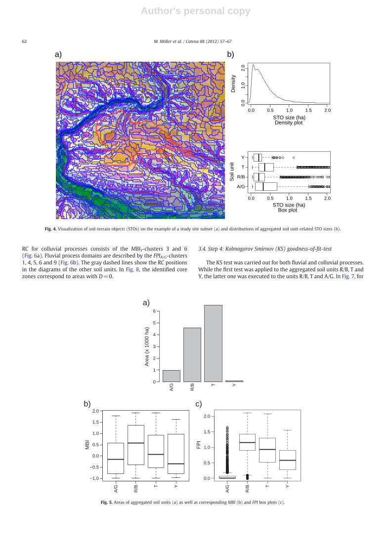
The blue-framed objects in Fig. 4a represent STOs which subdividea red-framed superior VBK 50 unit. The STOs vary in size dependingon their terrain position. This corresponds to the soil unit-related dis-tributions of STO sizes (Fig. 4b): While the units T and A/G occur inrather flat areas (green and orange-colored STOs), the units R/B andY are connected to steeper areas (magenta and blue-colored STOs).

The data integration process results in soil unit-related FPI andMBI distributions (Fig. 5b and c). All medians show typical positionswithin FPI and MBI value ranges. This is particularly true for mediansof A/GFPI and YMBI which are minimal and confirm the assumptions inSection 3.1. However, all distributions are characterized by overlapsand wide value ranges.

3.3. Step 3: Cluster analysis and identification of reference clusters

As already stated in Section 2.2.3, K-means clustering requires de-termination of the desired cluster number. Here, the FPI and MBI fea-ture space of each aggregated soil unit was subdivided into tenclusters, and twenty iterations were run for each clustering. InFig. 6, the associated FPI and MBI box plots as well as their positionswithin FPI and MBI value ranges are visualized. The vertical red andblue solid lines correspond to the upper boundary of MBI and FPIvalue ranges which represent reference clusters (RC). RC can be con-sidered as core zones of fluvial and colluvial process domains. Theyare composed of clusters which were identified by expert knowledge.

2 http://www.r-project.org.3 http://stat.ethz.ch/R-manual/R-devel/library/stats/html/kmeans.html.4 http://stat.ethz.ch/R-manual/R-devel/library/stats/html/ks.test.html.



RC for colluvial processes consists of the MBIY-clusters 3 and 6(Fig. 6a). Fluvial process domains are described by the FPIA/G-clusters1, 4, 5, 6 and 9 (Fig. 6b). The gray dashed lines show the RC positionsin the diagrams of the other soil units. In Fig. 8, the identified corezones correspond to areas with D=0.

3.4. Step 4: Kolmogorov Smirnov (KS) goodness-of-fit-test

The KS test was carried out for both fluvial and colluvial processes.While the first test was applied to the aggregated soil units R/B, T andY, the latter one was executed to the units R/B, T and A/G. In Fig. 7, for

a)

0.0 0.5 1.0 1.5 2.0

0.0

1.0

2.0

Density plotSTO size (ha)

Den

sity

A/G

R/B

T

Y

0.0 0.5 1.0 1.5 2.0

Box plotSTO size (ha)

Soi

l uni

t

b)

Fig. 4. Visualization of soil-terrain objects (STOs) on the example of a study site subset (a) and distributions of aggregated soil unit-related STO sizes (b).

A/G

R/B T Y

Are

a (x

100

0 ha

)

0

1

2

3

4

5

6

a)

A/G

R/B T Y

−1.0

−0.5

0.0

0.5

1.0

1.5

2.0

MB

I

b)

A/G

R/B T Y

0.0

0.5

1.0

1.5

2.0

FP

I

c)

Fig. 5. Areas of aggregated soil units (a) as well as corresponding MBI (b) and FPI box plots (c).



each aggregated soil unit, all cluster-related ECDFs are plotted asblack graphs against the blue and red colored ECDF graphs of RC.ECDFs with differences Db1 are plotted as gray graphs. The associatedcluster number is labeled and can be connected with the listed Dvalues of Table 3. Although all p values denote significant differencesbetween RC and cluster-related distributions, small D values indicatesimilarities to colluvial or fluvial process domains.

In Fig. 8, the resulting D values are joined with STOs and mapped.Four groups of STOs arise (see also Fig. 2 and Section 2.2):

1. Level D=0 denotes STOR which were identified as reference clus-ters (RC). These core zones of colluvial and fluvial process domains(class C) are displayed in dark blue.

2. STOR with D=1 were rejected as reference clusters. They are redhighlighted and have to be newly classified (class Ni).

3. STOP with DN0 and Db1 indicate potential areas affected by fluvialor colluvial processes. With it, users can formulate a basis fordecision-making which STOP should be newly assigned to fluvialor colluvialprocess domains (class RPi). In doing so, the applicationof a classification rule (here DY≤0.38, DA/G≤0.49) would lead to arevised soil map with new soil unit-related FPI and MBI distribu-tions (see Table 3).

The boxplot comparison of the original (Fig. 5b and c) and testedsoil units demonstrates that value ranges of A/G and Y – whichwere identified as implausible – were removed and transferred into

−1.0 0.0 1.0 2.0

0.0

0.2

0.4

A/G

Density plot | N=1825MBI

Den

sity

−1.0 0.0 1.0 2.0

0.0

0.2

0.4

0.6

R/B


Den

sity

−1.0 0.0 1.0 2.0

0.0

0.2

0.4

T


Den

sity

−1.0 0.0 1.0 2.0

0.0

0.2

0.4

Y


Den

sity

RC

13

57

9

−1.0 0.0 1.0 2.0

Box plotMBI

−1.0 0.0 1.0 2.0

Box plotMBI

−1.0 0.0 1.0 2.0

Box plotMBI

−1.0 0.0 1.0 2.0

Box plotMBI

Clu

ster

13

57

9

Clu

ster

13

57

9

Clu

ster

13

57

9

Clu

ster

RC

a) Identification of colluvial reference cluster (RC) within the aggregated soil unit Y

0.0 0.5 1.0 1.5 2.0 0.0 0.5 1.0 1.5 2.0 0.0 0.5 1.0 1.5 2.0 0.0 0.5 1.0 1.5 2.0

05

1015

20

A/G

Density plot | N=1825FPI

Den

sity

RC

0.0

0.4

0.8

R/B


Den

sity

0.0

0.2

0.4

0.6

T


Den

sity

0.0

0.2

0.4

0.6

0.8

Y


Den

sity

13

57

9

0.0 0.5 1.0 1.5 2.0

Box plotFPI

0.0 0.5 1.0 1.5 2.0

Box plotFPI

0.0 0.5 1.0 1.5 2.0

Box plotFPI

0.0 0.5 1.0 1.5 2.0

Box plotFPI

Clu

ster

13

57

9

Clu

ster

13

57

9

Clu

ster

13

57

9

Clu

ster

b) Identification of fluvial reference cluster (RC) within the aggregrated soil unit A/G

Fig. 6. MBI and FPI density plots and cluster-related box plots for each aggregated soil unit. The vertical solid lines indicate reference clusters (RC) of colluvial (red) and fluvial pro-cess domains (blue). The gray dashed lines show the RC positions in the diagrams of the other soil units. (For interpretation of the references to color in this figure legend, the readeris referred to the web version of this article.)



the new classes ‘AG rejected’ and ‘Y rejected’ (Fig. 9b and c). Both cor-respond to class Ni of the workflow (Fig. 2). The classes A/G and Yconsist of confirmed (Ci) and positive tested STO clusters (RPi). Tand R/B correspond to negative tested clusters (Pi). Overlapping dis-tributions between the soil units A/G or Y and R/B or T could be min-imized. However, the remaining aggregated soil units A/G and Y stillshow overlapping distributions which were tested positive regardingboth existence of fluvial and colluvial process domains. This is an ex-pression of situations where both soil forming processes could takeplace and superimpose. This class is labeled as ‘A/G or Y’ and also cor-responds to class RPi of the workflow.

The comparison of original and revised A/G soil unit areas revealsan increase by almost half (Figs. 9a and 5a). The tenfold increase of

colluvial areas is caused by the specific thematic attribute structure ofthe older soil maps which formed the basis for the CSM creation (seeSection 1). There, smaller colluvial soil units are only documented inthe attribute table. This information has got lost during the semantictransformation. This means that the classification result represents ageometric disaggregation revealing semantic terrain-related informa-tion. The main source for the new assigned colluvial soils is the aggre-gated soil unit T (Tschernosem).

4. Discussion and conclusion

A main challenge of digital soil mapping (DSM) is the adoption ofappropriate techniques and input data for operational use. A key togain acceptance and overcome possible resistance is the developmentand application of standardized protocols for producing predictivemaps (Hengl and MacMillan, 2009; MacMillan, 2008). Againstthis background, the presented procedure can be considered as amodular structured framework for terrain-related plausibility testsof conceptual soil maps (CSM; see Fig. 2). Framework means thatall tests and the underlying methods can be adapted to specific testobjectives. In this article, the CSM of the German Federal State ofSaxony-Anhalt should be tested against their colluvial and fluvialplausibility. The applied procedure was exemplified on a test sitewith an area of about 100 km2 and consists of four steps:

1. In the first step, explaining relief parameters on demandwere calcu-lated for the identification offluvial and colluvial process domains. Indoing so, basic relief parameters were combined to the FloodplainIndex (FPI) and Mass Balance Index (MBI) allowing a relative charac-terizing of process domains. As shown by Möller et al. (2008), the

1.0

0.8

0.6

0.4

0.2

0.0

1.0

0.8

0.6

0.4

0.2

0.0

1.0

0.8

0.6

0.4

0.2

0.0

Em

piric

al C

DF

1.0

0.8

0.6

0.4

0.2

0.0

1.0

0.8

0.6

0.4

0.2

0.0

1.0

0.8

0.6

0.4

0.2

0.0

Em

piric

al C

DF

A/G R/B

R/B

T

T

-1.0 0.0 0.5 1.0 1.5 2.0

MBI-1.0 0.0 0.5 1.0 1.5 2.0

MBI-1.0 0.0 0.5 1.0 1.5 2.0

MBI

0.0

0.5

1.0

1.5

2.0 0.0 0.5 1.0 1.5 2.0

FPI FPI

0.0 0.5 1.0 1.5 2.0

FPI

Y

a) Test for colluvial plausibility

b) Test for fluvial plausibility

RC

RCRC RC

4 1 8 4 9 6

RC RC

12 10 7 757 6

Fig. 7. ECDF plot comparison of reference clusters (RC) and soil unit-related MBI and FPI clusters. Blue colored graphs indicate fluvial process domains, and red colored RC graphsstand for colluvial process domains. ECDF plots with Db1 are gray colored and labeled with the associated cluster number of Table 3. (For interpretation of the references to color inthis figure legend, the reader is referred to the web version of this article.)

Table 3D values between reference clusters (RC) and soil unit-related MBI and FPI clusters(see Fig. 7). Values of Db1 are gray and values of Db0.5 are bold emphasized.

Aggregated 1 4 5 6 7 8 9 10

soilunit MBI clusters

A/G 0.38*

2 3

0.68* 1* 1* 0.96* 0.67* 1* 1*

R/B 1* 0.72* 1* 1* 1* 1* 0.31*

T 1*

1*

1* 1* 0.32* 1* 0.69* 1* 1*

1*

1*

1*

1*

1*

FPIclusters

R/B 0.99* 0.39* 1* 1* 1* 1*

T 1* 0.95* 1* 0.30* 1* 1*

Y 1*

1*1*

1* 1* 0.94* 1* 0.49* 1*

1*

1*

1*

1*

1*

1*

1*

1*

1*

⁎ Significance level pb0.01.



MBI value distribution can be affected by changing the transfer con-stant F enabling smoothing and emphasizing of landforms (seeEqs. (5) and (7)). Thus, an adaptation of test results to available inde-pendent reference information is possible.

2. Both CSM spatial domain and the explaining relief parametershad to be integrated in the second step. This was done by theapplication of a hierarchical region-growing segmentation al-gorithm applied on basic relief parameters considering already

existing CSM boundaries. A positive side-effect of segmentationis the reduction of data volume which becomes important forlarge data sets. Here, the data volume was reduced to onetenth.

3. In fact, clustering is a special case of segmentation in which onlyneighboring relations in the feature space are considered. Here,the one-dimensional feature spaces of MBI or FPI were grouped.We have preferred the K-means algorithm because the user can

Fig. 8. Visualization of D value levels resulting from plausibility tests (see Table 3).A

/G

A/G

or

Y

A/G

rej

ecte

d

R/B T Y

Y r

ejec

ted

Are

a (x

100

0 ha

)

0

1

2

3

4

5

6

a)

A/G

A/G

or

Y

R/B T Y

Y r

ejec

ted

−1.0

−0.5

0.0

0.5

1.0

1.5

2.0

MB

I

b)

A/G

A/G

or

Y

A/G

rej

ecte

d

R/B T Y

0.0

0.5

1.0

1.5

2.0

FP

I

c)

Fig. 9. Areas of test result classes (a) as well as corresponding MBI (b) and FPI box plots (c). A/G and Y consist of confirmed (Ci) and positive tested STOR clusters (RPi; see Fig. 2).T and R/B correspond to negative tested STOP clusters (Pi). The classes ‘A/G rejected’ and ‘Y rejected’ are negative tested STOR clusters (Ri) and are equivalent to class (Ni). The class‘A/G or Y’ represents overlapping distributions of A/G or Y which were tested positive regarding both existence of fluvial and colluvial process domains (RPi).



control the degree of feature space aggregation through the deter-mination of the cluster number. However, the algorithm can besubstituted by other approaches which, for instance, enable an au-tomatic determination of cluster number (e.g. Fraley and Raftery,2007).

4. The applied Kolmogorov Smirnov (KS) test is a traditionalgoodness-of-fit test calculating the distance D between two em-pirical cumulative distribution functions (ECDF). Because of itsstatistical robustness the KS test proved to be suitable for thecomparison of soil- and terrain-related distributions. Especially,the insensitiveness to different STO numbers of the comparingdistributions is important for the transfer to larger areas. In thefuture, ECDF-based alternatives to the KS test (see Thas, 2010)will be evaluated.

The presented approach can help to form an impression concern-ing the terrain-related plausibility of CSM or also legacy soil mapswhich oftentimes do not contain any accuracy information. Plausibil-ity is expressed here by the distance between reference clusters (RC)and soil unit-related clusters (Pi) which should be tested (see Fig. 2).The most crucial point of the workflow is the expert-based RC selec-tion representing “true” process domain of interest. However, inspite of the operation's subjectivity, the selection process itself isdone deliberately and controlled and thus, traceable.

In a more general sense, the applied methodology of data integra-tion is suitable for adopting existing data in computer-based systems.The data integration approach is based on the coupling of existingfunctional hierarchies of thematic geodata (here: a CSM) and multi-scale object structures (Möller et al., 2008). Multi-scale object struc-tures arise from the region-based segmentation of continuousdata (here: basic relief parameters). The resulting soil-terrain unitsenable a supervised disaggregation of heterogeneous soil units (seeWielemaker et al., 2001). Supervised disaggregation means that theapplied segmentation algorithm leads to STOs representing a specificgeometric aggregation level. The classification of the testing resultscomplies with a semantic disaggregation.

Finally, the test modules may be used for the supervised selection ofappropriate samples for automatic classification algorithms (Behrensand Scholten, 2006; Grunwald, 2009; MacMillan, 2008; Scull et al.,2003). Similar to instance selection techniques (Behrens et al., 2008;Schmidt et al., 2008), training data sets might be cleaned from noisydata.

Acknowledgements

The authors wish to thank Dr. Martin Volk, Dr. Carsten Dormann(both from Helmholtz Centre for Environmental Research — UFZ, De-partment Computational Landscape Ecology, Leipzig) and MichaelBock (Scilands GmbH/University of Hamburg, Department of PhysicalGeography) for discussion and helpful comments. We are also verygrateful to an unknown reviewer who provided valuable advice onhow to improve significantly the manuscript.

References

Ad-hoc AG, Boden, 2005. Bodenkundliche Kartieranleitung (KA 5), 5th Edition. E.Schweizerbart'sche Verlagsbuchhandlung, Stuttgart, Germany.

Albrecht, C., Jahn, R., Huwe, B., 2005. Bodensystematik und Bodenklassifikation — Teil1: Grundbegriffe. Journal of Plant Nutrition Soil Science 168 (1), 7–20.

Baatz, M., Schäpe, A., 2000. Multiresolution segmentation: an optimization approachfor high quality multi-scale image segmentation. In: Strobl, J., Blaschke, T. (Eds.),Angewandte Geographische Informationsverarbeitung — Beiträge zum AGIT-Syposium. Vol. 12. Salzburg, pp. 12–23.

Behrens, T., Scholten, T., 2006. A comparison of data-mining techniques in predictive soilmapping. In: Lagacherie, P., A.M., Voltz, M. (Eds.), Digital SoilMapping— an Introduc-tory Perspective. Vol. 31 of Developments in Soil Science. Elsevier, pp. 353–364.

Behrens, T., Schmidt, K., Scholten, T., 2008. An approach to removing uncertainties innominal environmental covariates and soil class maps. In: Hartemink, A., McBratney,

A., Mendonça Santos, M. (Eds.), Digital Soil Mapping with Limited Data. Springer,pp. 213–224.

Brenning, A., 2008. Statistical geocomputing combining R and SAGA: the example oflandslide susceptibility analysis with generalized additive models. In: Böhner, J.,Blaschke, T., Montanarella, L. (Eds.), SAGA — seconds out. Vol. 19 of HamburgerBeiträge zur Physischen Geographie und Landschaftsökologie, pp. 23–32.

Bui, E.N., 2004. Soil survey as a knowledge system. Geoderma 120 (1–2), 17–26.Buol, S., Southard, R., Graham, R., McDaniel, P., 2003. Soil Genesis and Classification, 5th

Edition. Iowa State Press, Ames, Iowa.Davis, J., 2002. Statistics and Data Analysis in Geology. John Wiley & Sons, New York.Deumlich, D., Thiere, J., Frielinghaus, M., Voelker, L., 1998. MMK characterisation and

classification of site conditions in the new federal states of Germany. In: Heineke,H., Eckelmann, W., Thomasson, A., Jones, R., Montanarella, L., Buckley, B. (Eds.),Land Information Systems — Developments for planning the sustainable useof land resources. Vol. 4 of European Soil Bureau Research Report, EUR 17729EN. Office for Official Publications of the European Communities, Luxembourg,pp. 473–478.

Deumlich, D., Schmidt, R., Sommer, M., 2010. Amultiscale soil–landform relationship inthe glacial-drift area based on digital terrain analysis and soil attributes. Journal ofPlant Nutrition and Soil Science 173 (6), 843–851.

Dobos, E., Hengl, T., 2009. Soil mapping applications. In: Hengl, T., Reuter, H. (Eds.),Geomorphometry — concepts, Software, Applications. Vol. 33 of Developments inSoil Science. Elsevier, pp. 461–479.

Dragut, L., Blaschke, T., 2006. Automated classification of landform elements usingobject-based image analysis. Geomorphology 81 (3–4), 330–344.

Dragut, L., Eisank, C., 2011. Object representations at multiple scales from digital eleva-tion models. Geomorphology 129 (3–4), 183–189.

Dragut, L., Schauppenlehner, T., Muhar, A., Strobl, J., Blaschke, T., 2009. Optimization ofscale and parametrization for terrain segmentation: an application to soil-landscape modeling. Computers and Geosciences 35 (9), 1875–1883.

Fraley, C., Raftery, A., 2007. Model-based methods of classification: using the mclustSoftware in Chemometrics. Journal of Statistical Software 18, 419–430.

Friedrich, K., 1996. Digitale Reliefgliederungsverfahren zur Ableitung bodenkundlichrelevanter Flächeneinheiten. Vol.21 of Frankfurter Geowissenschaftliche Arbeiten.Frankfurt (Main).

Friedrich, K., 1998. Multivariate distance methods for geomorphographic relief classifi-cation. In: Heinecke, H., Eckelmann, W., Thomasson, A., Jones, J., Montanarella, L.,Buckley, B. (Eds.), Land information systems— developments for planning the sus-tainable use of land resources. Vol. 4 of European Soil Bureau Research Report, EUR17729 EN. Office for official publications of the European Communities, Luxembourg,pp. 259–266.

Grunwald, S., 2009. Multi-criteria characterization of recent digital soil mapping andmodeling approaches. Geoderma 152 (3/4), 195–207.

Hartmann, K.-J., 2005. Bereitstellung von Informationen der bodenkundlichen Lande-saufnahme zur Bewertung von Bodenfunktionen. In: Möller, M., Helbig, H. (Eds.),GIS-gestützte Bewertung von Bodenfunktionen – Datengrundlagen und Lösung-sansätze. Wichmann, Heidelberg, pp. 27–34.

Hartmann, K.-J., 2006. Bodenkundliche Basisinformationen. In: Feldhaus, D., Hartmann, K.-J.(Eds.), Bodenbericht 2006 – Böden und Bodeninformationen in Sachsen-Anhalt. Vol.11ofMitteilungen zuGeologie und Bergwesen in Sachsen-Anhalt. Landesamt für Geologieund Bergwesen Sachsen-Anhalt, Halle (Saale), pp. 71–88.

Hastie, T., Tibshirani, R., Friedman, J., 2009. The Elements of Statistical Learning: DataMining, Inference and Prediction, 2nd Edition. Springer Series in Statistics.Springer, New York.

Hengl, T., MacMillan, R., 2009. Geomorphometry – A key to landscape mapping andmodelling. In: Hengl, T., Reuter, H. (Eds.), Geomorphometry - Concepts, Software,Applications. Vol.33 of Developments in Soil Science. Elsevier, pp. 433–460.

Hutchinson, M., 1989. A new procedure for gridding elevation and stream line datawith automatic removal of spurious pits. Journal of Hydrology 106, 211–232.

ISO 19138, 2006. Geographic information: Data quality measures. Tech. rep. Interna-tional Organization for Standardization, Geneve, Switzerland.

IUSS Working Group WRB, 2006. World Reference Base for Soil Resources, 2nd ed. FAO,Rome.

MacMillan, R., 2008. Experiences with applied DSM: Protocol, availability, quality andcapacity building. In: Hartemink, A., McBratney, A., Mendonça Santos, M. (Eds.),Digital Soil Mapping with limited data. Springer, pp. 113–135.

MacMillan, R., Shary, P., 2009. Landforms and landform elements in geomorphometry.In: Hengl, T., Reuter, H. (Eds.), Geomorphometry - Concepts, Software, Applica-tions. Vol.33 of Developments in Soil Science. Elsevier, pp. 227–254.

Minár, J., Evans, I., 2008. Elementary forms for land surface segmentation: The theoret-ical basis of terrain analysis and geomorphological mapping. Geomorphology 95(3–4), 236–259.

Möller, M., 2008. Scale-specific derivation of thematic basic data for landscape analysis.Ph.D. thesis. University of Tübingen, Tübingen, Germany, in German.

Möller, M., Volk, M., Friedrich, K., Lymburner, L., 2008. Placing soil genesis and trans-port processes into a landscape context: A multi-scale terrain analysis approach.Journal of Plant Nutrition and Soil Science 171, 419–430.

Müller, E., Volk, M., 2001. History of landscape assessment. In: Krönert, R., Steinhardt,U., Volk, M. (Eds.), Landscape balance and landscape assessment. Spinger, Berlin,pp. 23–46.

Olaya, V., Conrad, O., 2009. Geomorphometry in SAGA. In: Hengl, T., Reuter, H. (Eds.),Geomorphometry - Concepts, Software, Applications. Vol.33 of Developments inSoil Science. Elsevier, pp. 293–308.

Quinn, P., Beven, K., Lamb, R., 1995. The ln(a/tan b) index: How to calculate it andhow to use ist within the TOPMODEL framework. Hydrological Processes 9,161–182.



Schmidt, K., Behrens, T., Scholten, T., 2008. Instance selection and classification treeanalysis for large spatial datasets in digital soil mapping. Geoderma 146 (1–2),138–146.

Scull, P., Franklin, J., Chadwick, O.A., McArthur, D., 2003. Predictive soil mapping: A re-view. Progress in Physical Geography 27 (2), 171–197.

Thas, O., 2010. Comparing Distributions. Springer Series in Statistics, Springer,New York.

Wielemaker, W.G., de Bruin, S., Epema, G.F., Veldkamp, A., 2001. Significance and appli-cation of the multi-hierarchical landsystem in soil mapping. Catena 43 (1), 15–34.

Zevenbergen, L., Thorne, C., 1987. Quantitaive analysis of land surface topography.Earth Surface Processes and Landforms 12, 12–56.


Plausibility test of conceptual soil maps using relief parameters

Documents