Welcome message from author
This document is posted to help you gain knowledge. Please leave a comment to let me know what you think about it! Share it to your friends and learn new things together.
Transcript

Abstract
Vehicular Ad Hoc Networks (VANETs) are envisioned to support three types of applications:
safety, traffic management, and commercial applications. By using wireless interfaces to form an
ad hoc network, vehicles will be able to inform other vehicles about traffic accidents, potentially
hazardous road conditions, and traffic congestion. Commercial applications are expected to
provide incentive for faster adoption of the technology.
To date, VANET research efforts have relied heavily on simulations, due to prohibitive
costs of deploying real world testbeds. Furthermore, the characteristics of VANET protocols
and applications, particularly those aimed at preventing dangerous situations, require that the
initial testing and evaluation be performed in a simulation environment before they are tested
in the real world where their malfunctioning can result in a hazardous situation.
Existing channel models implemented in discrete-event VANET simulators are by and large
simple stochastic radio models, based on the statistical properties of the chosen environment,
thus not accounting for the specific obstacles in the region of interest. It was shown in [1] and [2]
that such models are unable to provide satisfactory accuracy for typical VANET scenarios.
While there have been several VANET studies recently that introduced static objects (e.g.,
buildings) into the channel modeling process, modeling of mobile objects (i.e., vehicles) has
been neglected. We performed extensive measurements in different environments (open space,
highway, suburban, urban, parking lot) to characterize in detail the impact that vehicles have
on communication in terms of received power, packet delivery rate, and effective communication
range. Since the impact of vehicles was found to be significant, we developed a model that
accounts for vehicles as three-dimensional obstacles and takes into account their impact on the
line of sight obstruction, received signal power, packet reception rate, and message reachability.
The model is based on the empirically derived vehicle dimensions, accurate vehicle positioning,
i
ii
and realistic mobility patterns. We validate the model against measurements and it exhibits
realistic propagation characteristics while maintaining manageable complexity.
In highway environments, vehicles are the most significant source of signal attenuation and
variation. In urban and suburban environments, apart from vehicles, static objects such as
buildings and foliage have a significant impact on inter-vehicle communication. Therefore, to
enable realistic modeling in urban and suburban environments, we developed a model that
incorporates static objects as well. The model requires minimum geographic information: the
location and the dimensions of modeled objects (vehicles, buildings, and foliage). We validate the
model against measurements and show that it successfully captures both small-scale and large-
scale propagation effects in different environments (highway, urban, suburban, open space).
Finally, we performed experiments which showed that selecting tall vehicles as next-hop re-
lays is beneficial in terms of higher power at the receiver, smaller number of hops to reach the
destination, and increased per-hop communication range. Based on these results, we designed
a technique that utilizes the advantageous position of antennas on tall vehicles (e.g., buses,
trucks) to relay the messages. The technique improves communication performance by decreas-
ing the number of hops needed to reach the destination, thus reducing the end-to-end delay and
increasing the effective communication range.
Resumo
As redes veiculares (VANETs) estao preparadas para suportar pelo menos tres tipos de aplicacoes:
disseminacao de informacoes de seguranca, gestao de trafego, e aplicacoes comerciais. Recor-
rendo a interfaces radio sem fios para formar uma rede ad hoc, os veıculos serao capazes de
informar outros veıculos sobre acidentes, condicoes de estrada potencialmente perigosas, e con-
gestionamentos. Ao mesmo tempo, espera-se que as aplicacoes comerciais fornecam os incentivos
economicos para uma rapida adocao da tecnologia.
Ate agora, as avaliacao do desempenho de redes veiculares basearam-se principalmente em
simulacoes, devido aos custos proibitivos na implementacao de testbeds reais. Alem disso, as
caracterısticas dos protocolos e aplicacoes para redes veiculares, em particular aquelas destinadas
a prevencao de situacoes perigosas, exigem que os testes iniciais se realizem por simulacao antes
de serem aplicadas no mundo real, uma vez que o seu mau funcionamento pode causar situacoes
de perigo.
Os modelos actuais de canais de comunicacao implementados em simuladores sao, no geral,
modelos probabilısticos simplificados que se baseiam numa caracterizacao estatıstica do cenario
a ser analisado e, por consequente, nao incorporam os obstaculos especıficos presentes na regiao
de interesse. Estudos em [1] e [2] mostraram que tais modelos sao incapazes de fornecer uma
precisao satisfatoria em cenarios VANET tıpicos.
Embora varios estudos recentes em VANETs tenham introduzido objetos estaticos (por ex-
emplo, edifıcios) no processo de modelacao do canal, a modelacao de objetos moveis, nomeada-
mente veıculos, tem sido negligenciada. Neste trabalho foram realizadas medicoes em diferentes
ambientes (espaco aberto, autoestrada, suburbano, urbano, parque de estacionamento) para
caracterizar em detalhe o impacto que os veıculos tem na comunicacao em termos do nıvel de
potencia do sinal recebido, da taxa de entrega de pacotes, e do raio de alcance efetivo da comu-
iii
iv
nicacao. Uma vez que o impacto dos veıculos se mostrou significativo, propomos um modelo que
abstrai os veıculos como obstaculos tridimensionais e leva em consideracao o seu impacto sobre
a linha de vista entre o transmissor e o receptor, a potencia do sinal que chega ao receptor, a
taxa de entrega de pacotes, e o alcance dos mesmos na rede. O modelo baseia-se nas dimensoes
do veıculo, no posicionamento do veıculo, e em padroes de mobilidade realistas, todos obtidos
empiricamente. Os resultados previstos pelo modelo sao comparado com os resultados obtidos
atraves de medicoes, sendo observada uma boa concordncia entre ambos.
Em ambientes de estrada, os veıculos sao a fonte mais significativa de atenuacao do sinal.
Em ambientes urbanos e suburbanos, para alem de veıculos, objetos estaticos como edifıcios e a
vegetacao tem um impacto sobre a comunicacao inter-veıculos. Portanto, e para permitir uma
modelacao do canal realista em ambientes urbanos e suburbanos, este trabalho apresenta um
modelo que incorpora os objetos estaticos supracitados. O modelo requer informacao geografica
mınima: 1) informacao sobre a localizacao do veıculos; e 2) informacao sobre os contornos
dos objetos estaticos. O modelo e validado por comparacao com resultados experimentais, e
demonstra-se que e capaz de capturar com sucesso os efeitos da atenuacao e propagacao em
larga escala em diferentes cenarios (autoestrada, urbano, suburbano, espaco aberto).
Finalmente, realizaram-se testes que mostraram que a escolha de veıculos altos como nos
principais para reencaminhamento de mensagens e benefico em termos de uma maior forca de
sinal no receptor, menor nmero de saltos ate atingir o destino, e mais alcance de comunicacao
por salto. Com base nesses resultados, e proposta uma tecnia que tira vantagem da posicao
elevada das antenas em veıculos altos (como autocarros e camioes) para o encaminhamento de
mensagens. A tecnica proposta melhora o desempenho das comunicacoes, diminuindo o nmero de
saltos necessario para chegar ao destino, reduzindo assim o atraso total fim-a-fim e aumentando
o alcance efetivo das comunicacoes.

v
This is for Shesha
Acknowledgements
This thesis was made possible through the selfless support of a great number of people.
First, I would like to thank my advisors, Prof. Ozan K. Tonguz and Prof. Joao Barros.
I joined Ozan’s group at CMU back in 2007 as a Fulbright scholar. I was supposed to spend
eight months at CMU – five years later, here I am writing the acknowledgements for my thesis.
While my journey has been long and winding, Ozan was always there to give me valuable
advice. He instilled in me the scientific method and the rigorous approach to research, while
also encouraging me to pursue out-of-the-box ideas. His ability to scope the problem and express
it in simple terms is the ideal I strive for in my own research. When I officially started my Ph.D.
in early 2009, I joined Joao’s group. With his unique enthusiasm and energy, Joao brought a
new dimension to my research. His unparalleled ability to get things done enabled me to pursue
research directions that would otherwise remain inaccessible to me. Joao’s support was key in
enabling me to perform the experimental part of my work. Furthermore, his open approach to
research allowed me to collaborate with some brilliant people that enriched both my knowledge
and this thesis. Ozan and Joao have also taught me the subtle differences between well-written,
focused, and ambiguous, uninspiring scientific prose.
The ability to identify research problems is the skill that defines an independent researcher.
Since the goal of the Ph.D. is to educate independent researchers, I am most grateful to my
advisors for giving me the complete freedom to find and go after the research problems that I
considered interesting, at the same time keeping a keen eye on me so I do not get sidetracked.
Next, I would like to thank Prof. Peter Steenkiste, Prof. Ana Aguiar and Prof. Vijayakumar
Bhagavatula for agreeing to serve on my defense committee. They provided invaluable advice
which considerably improved the quality of this thesis. I am grateful to Prof. Steenkiste for his
insightful advice during our collaboration over the past two and a half years. This thesis as a
vi
vii
whole, and the experimental work contained within it in particular, has benefited greatly from
his deep knowledge of wireless networking and experimental methods. Prof. Aguiar’s expertise
in the areas of simulation and measurements resulted in a more rigorous performance evaluation
of the models developed in this thesis. Additionally, Prof. Aguiar participated in one of the
measurement campaigns, results of which are used in this thesis. Despite his many obligations,
including acting as a Dean of the College of Engineering, Prof. Bhagavatula kindly accepted to
serve on my committee. I am deeply grateful for his valuable time and technical advice.
I was fortunate to collaborate closely with Dr. Tiago T. V. Vinhoza and Rui Meireles. I
learned a great deal from Tiago about the physical layer, wireless communication, and the
mathematical underpinnings of communications. Tiago is a careful listener with an ability to
explain, in so many words, when the ideas are worth pursuing and also when they are off target.
His incredible attention to detail and encyclopedic knowledge of all things EE made it a real
pleasure to hang out with him at the white board and collaborate on projects that form the core
of this thesis. Also, I am most grateful to him for proofreading the early drafts of this thesis.
Rui was my companion in virtually all measurement campaigns and the cowriter of the ensuing
papers. Driving countless times around the same route during rush hours, in the middle of the
night, and on weekends in cheap rental cars to collect enough measurement data is nobody’s idea
of a good time. Rui’s composure, organizational ability, and extensive knowledge of protocols
and scripting enabled us to stay on track both literally and figuratively.
I would like to express my gratitude to Prof. Michel Ferreira, who provided the aerial pho-
tography which enabled a thorough investigation into the impact of vehicular obstructions. He
also participated in the design of the model for vehicles as obstacles, as well as in the initial
discussions during which the tall vehicle relaying idea was formed.
I am indebted to Prof. Blazenka Divjak and Antun Brumnic at the University of Zagreb,
whose encouragement and support in my decision to study abroad was unwavering. Blazenka
helped me to apply for the Fulbright scholarship and has supported me ever since in more
ways than I could possibly recollect. Even when it meant confronting the powers that be, she
stood by my side. Throughout the past seven years, Antun provided me with constant advice
when I needed it the most. Every time I was at the crossroads and needed to make a difficult
decision, he told me exactly what I needed to hear to make the right decision. His integrity and
uncompromising dedication have been an inspiration for me.
viii
My labmates at the University of Porto were a joy to be around. For countless conversations
next to the coffee machine, ranging from complaints about the daily grind to space travel, but
most often converging to sports and politics, I would like to thank Tiago Vinhoza, Joao Almeida,
Saurabh Shintre, Ian Marsh, Rui Costa, Paulo Oliveira, Pedro Santos, Sergio Crisostomo, and
Diogo Ferreira. For all the pleasant conversations not involving sports and politics, I would like
to thank Joao Paulo Vilela, Maricica Nistor, Gerhard Maierbacher, Traian Abrudan, and Hana
Khamfroush. Special thanks are also due to the my labmates at CMU for helping me to ease the
pressure of graduate life at CMU. In particular, I would like to thank Wantanee Viriyasitavat
(for helping out on numerous occasions, including proofreading my thesis and asking the right
questions during my practice talks), Jiun-Ren Lin (for taking time to provide useful feedback on
my practice talks and helping me with the thesis defense logistics, among many other things),
Hsin-Mu (Michael) Tsai (for his wise advice and brilliantly sharp questions that improved my
research), and Vishnu Naresh Boddeti (for our bike trips to and from DC and for numerous
enjoyable chats over the years). Amir Moghimi, Paisarn Sonthikorn, Yi Zhang, and Xindian
Long were always there when I needed advice during my first year at CMU. I would also like to
thank Paulo Oliveira, Xiaohui (Eeyore) Wang, Carlos Pereira, and Shshank Garg, fellow students
who set time apart from their busy schedules to help perform the experiments by driving a silly
number of times around the same locations. To all the soccer folks that are either listed above or
remain unnamed, I thank for playing the beautiful game, thus keeping me sane by occasionally
taking my mind off research.
My Ph.D. studies were funded by a grant from the Portuguese Foundation for Science and
Technology under the Carnegie Mellon | Portugal program (grant SFRH/BD/33771/2009) and
the DRIVE-IN project (CMU-PT/NGN/0052/2008).
I would have not been able to focus on my graduate studies if it were not for the unconditional
love and support of my family. My sincerest gratitude goes to my mother and father, for instilling
in me the courage and allowing me to take my own path, even at times when they did not agree
with my choice. Despite the physical distance between us during the last five years, I always
felt their support. I would also like to thank my grandparents, in particular my late grandfather
Ljubo. Through the vivid example of his own life, he has showed me the value of hard work,
perseverance, and integrity.
Finally, I would like to thank my wife Sanja. Words cannot express the gratitude I feel for

ix
the love and support she has given me. She was my companion, best friend, and a source of
inspiration throughout the last six and a half years. Every time I was down, she found a way
to lift me up, always with a kind word of support, even during times when she was the one
suffering much more. As a small token of appreciation, with all my love I dedicate this thesis to
Sanja.
Contents
Abstract i
Resumo iii
1 Introduction 1
1.1 Motivation . . . . . . . . . . . . . . . . . . . . . . . . . . . . . . . . . . . . . . . 1
1.2 Thesis Organization . . . . . . . . . . . . . . . . . . . . . . . . . . . . . . . . . . 5
2 Experimental Evaluation of Vehicles as Obstructions 6
2.1 Motivation . . . . . . . . . . . . . . . . . . . . . . . . . . . . . . . . . . . . . . . 6
2.2 Experiment Setup . . . . . . . . . . . . . . . . . . . . . . . . . . . . . . . . . . . 9
2.2.1 Network Configuration . . . . . . . . . . . . . . . . . . . . . . . . . . . . . 9
2.2.2 Scenarios . . . . . . . . . . . . . . . . . . . . . . . . . . . . . . . . . . . . 10
2.3 Results . . . . . . . . . . . . . . . . . . . . . . . . . . . . . . . . . . . . . . . . . . 11
2.3.1 Parking lot experiments . . . . . . . . . . . . . . . . . . . . . . . . . . . . 11
2.3.2 On-the-road experiments . . . . . . . . . . . . . . . . . . . . . . . . . . . 12
2.4 Related Work . . . . . . . . . . . . . . . . . . . . . . . . . . . . . . . . . . . . . . 15
2.5 Conclusions . . . . . . . . . . . . . . . . . . . . . . . . . . . . . . . . . . . . . . . 16
3 Modeling Vehicles as Obstacles in VANETs 22
3.1 Motivation . . . . . . . . . . . . . . . . . . . . . . . . . . . . . . . . . . . . . . . 23
3.2 Related Work . . . . . . . . . . . . . . . . . . . . . . . . . . . . . . . . . . . . . . 25
3.2.1 Non-Geometrical Stochastic Models . . . . . . . . . . . . . . . . . . . . . 26
3.2.2 Geometry-Based Deterministic Models . . . . . . . . . . . . . . . . . . . . 26
3.2.3 Geometry-Based Stochastic Models . . . . . . . . . . . . . . . . . . . . . . 27
x

CONTENTS xi
3.3 Model Analysis . . . . . . . . . . . . . . . . . . . . . . . . . . . . . . . . . . . . . 28
3.3.1 The Impact of Vehicles on Line of Sight . . . . . . . . . . . . . . . . . . . 28
3.3.2 The Impact of Vehicles on Signal Propagation . . . . . . . . . . . . . . . . 31
3.4 Model Requirements . . . . . . . . . . . . . . . . . . . . . . . . . . . . . . . . . . 33
3.4.1 Determining the exact position of vehicles and the inter-vehicle spacing . 33
3.4.2 Determining the speed of vehicles . . . . . . . . . . . . . . . . . . . . . . . 33
3.4.3 Determining the vehicle dimensions . . . . . . . . . . . . . . . . . . . . . 34
3.5 Results . . . . . . . . . . . . . . . . . . . . . . . . . . . . . . . . . . . . . . . . . . 35
3.5.1 Probability of Line of Sight . . . . . . . . . . . . . . . . . . . . . . . . . . 37
3.5.2 Received Power . . . . . . . . . . . . . . . . . . . . . . . . . . . . . . . . . 40
3.5.3 Experimental Evaluation . . . . . . . . . . . . . . . . . . . . . . . . . . . 42
3.6 Conclusions . . . . . . . . . . . . . . . . . . . . . . . . . . . . . . . . . . . . . . . 45
4 Vehicle-to-Vehicle Channel Model for VANET Simulations 47
4.1 Motivation . . . . . . . . . . . . . . . . . . . . . . . . . . . . . . . . . . . . . . . 47
4.2 Experiment Setup . . . . . . . . . . . . . . . . . . . . . . . . . . . . . . . . . . . 49
4.3 Spatial Tree Structure for Efficient Object Manipulation . . . . . . . . . . . . . . 53
4.4 Description of the Channel Model . . . . . . . . . . . . . . . . . . . . . . . . . . . 55
4.4.1 Classification of link types . . . . . . . . . . . . . . . . . . . . . . . . . . . 57
4.4.2 Rules for reducing the computational complexity of the model . . . . . . 57
4.4.3 Transmission through Foliage . . . . . . . . . . . . . . . . . . . . . . . . . 59
4.4.4 Combining multiple paths: E-field and received power calculations . . . . 59
4.4.5 Practical considerations for different link types and propagation mechanisms 61
4.4.6 Small-scale signal variations . . . . . . . . . . . . . . . . . . . . . . . . . . 65
4.4.7 Assumptions . . . . . . . . . . . . . . . . . . . . . . . . . . . . . . . . . . 70
4.4.8 Channel Model Simulation Structure . . . . . . . . . . . . . . . . . . . . . 73
4.5 Results . . . . . . . . . . . . . . . . . . . . . . . . . . . . . . . . . . . . . . . . . . 73
4.5.1 LOS Links . . . . . . . . . . . . . . . . . . . . . . . . . . . . . . . . . . . 74
4.5.2 NLOSv Links . . . . . . . . . . . . . . . . . . . . . . . . . . . . . . . . . . 76
4.5.3 NLOSb Links . . . . . . . . . . . . . . . . . . . . . . . . . . . . . . . . . . 76
4.5.4 Combined large-scale and small-scale signal variation . . . . . . . . . . . . 80

CONTENTS xii
4.6 A Few Notes on the Performance of the Model . . . . . . . . . . . . . . . . . . . 80
4.7 Related Work . . . . . . . . . . . . . . . . . . . . . . . . . . . . . . . . . . . . . . 84
4.8 Conclusions . . . . . . . . . . . . . . . . . . . . . . . . . . . . . . . . . . . . . . . 87
5 TVR – Tall Vehicle Relaying 89
5.1 Motivation . . . . . . . . . . . . . . . . . . . . . . . . . . . . . . . . . . . . . . . 89
5.2 Model-Based Analysis of the Benefits of Tall Vehicles as Relays . . . . . . . . . . 91
5.2.1 Setup . . . . . . . . . . . . . . . . . . . . . . . . . . . . . . . . . . . . . . 91
5.2.2 Impact of Vehicles on Line of Sight . . . . . . . . . . . . . . . . . . . . . . 92
5.2.3 Difference Between Received Signal Strength for Tall and Short Vehicles . 92
5.3 Experimental Analysis of the Benefits of Tall Vehicles as Relays . . . . . . . . . 94
5.3.1 Experimental Scenarios . . . . . . . . . . . . . . . . . . . . . . . . . . . . 94
5.3.2 Hardware Setup . . . . . . . . . . . . . . . . . . . . . . . . . . . . . . . . 99
5.3.3 Experimental Results - One Hop Experiments . . . . . . . . . . . . . . . . 101
5.3.4 Experimental Results - Two Hop Experiments . . . . . . . . . . . . . . . 103
5.4 Large-scale Simulations . . . . . . . . . . . . . . . . . . . . . . . . . . . . . . . . 104
5.4.1 Relay Techniques Under Consideration . . . . . . . . . . . . . . . . . . . . 105
5.4.2 Calculating xmax . . . . . . . . . . . . . . . . . . . . . . . . . . . . . . . . 106
5.4.3 Comparing the Performance of the Relay Techniques . . . . . . . . . . . . 108
5.4.4 Properties of Selected Best-Hop Links . . . . . . . . . . . . . . . . . . . . 110
5.4.5 How Often is a Tall Vehicle Relay Available? . . . . . . . . . . . . . . . . 110
5.4.6 Does TVR Create Bottlenecks on Tall Vehicles? . . . . . . . . . . . . . . 113
5.5 Related Work . . . . . . . . . . . . . . . . . . . . . . . . . . . . . . . . . . . . . . 113
5.6 Conclusions . . . . . . . . . . . . . . . . . . . . . . . . . . . . . . . . . . . . . . . 115
6 Conclusion 117
6.1 Contributions . . . . . . . . . . . . . . . . . . . . . . . . . . . . . . . . . . . . . . 118
6.2 Future Work . . . . . . . . . . . . . . . . . . . . . . . . . . . . . . . . . . . . . . 119
List of Figures
1.1 Structure of the channel modeling subsection of VANET simulation environments 2
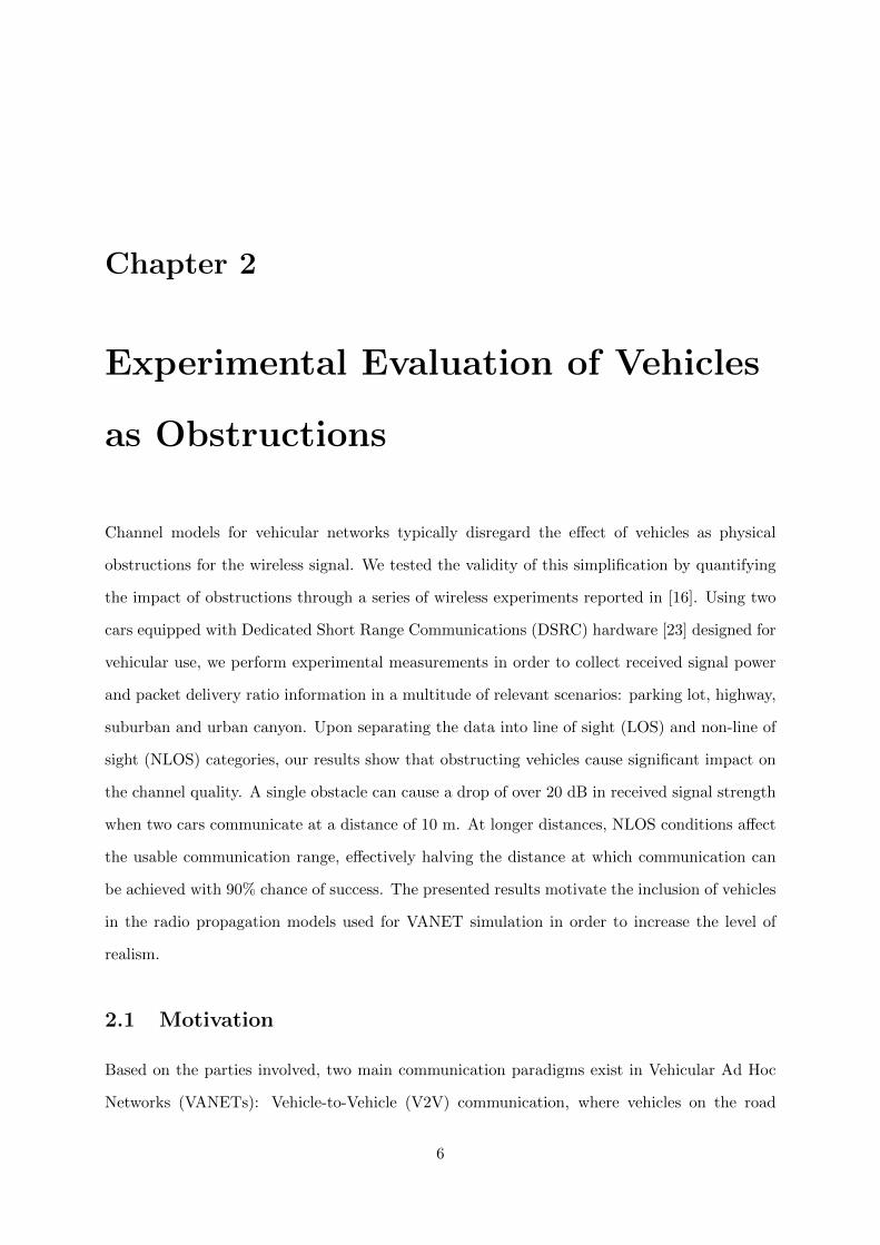
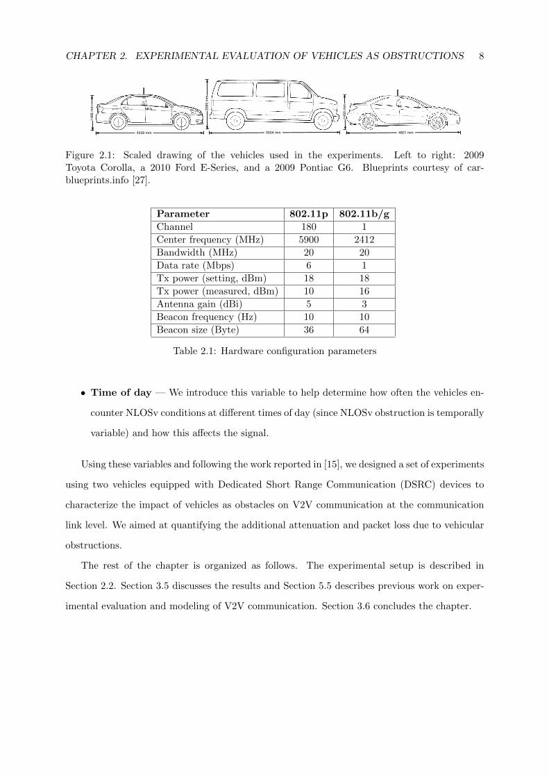
2.1 Scaled drawing of the vehicles used in the experiments . . . . . . . . . . . . . . . 8
2.2 Experimental setup. . . . . . . . . . . . . . . . . . . . . . . . . . . . . . . . . . . 18
2.3 Parking lot experiment results . . . . . . . . . . . . . . . . . . . . . . . . . . . . . 19
2.4 RSSI as a function of distance for LOS and NLOSv conditions . . . . . . . . . . 19
2.5 Packet delivery ratio: on-the-road experiments . . . . . . . . . . . . . . . . . . . 20
2.6 Reliable communication range . . . . . . . . . . . . . . . . . . . . . . . . . . . . . 20
2.7 Difference between the daytime and nighttime experiments . . . . . . . . . . . . 21
2.8 Received signal strength: on-the-road experiments . . . . . . . . . . . . . . . . . 21
3.1 Model for evaluating the impact of vehicles as obstacles on LOS . . . . . . . . . . 28
3.2 Speed and inter-vehicle spacing distribution on highways. . . . . . . . . . . . . . 36
3.3 Average number of neighbors with unobstructed and obstructed LOS on A28
highway. . . . . . . . . . . . . . . . . . . . . . . . . . . . . . . . . . . . . . . . . . 38
3.4 P (LOS) vs. observed range for different time offsets . . . . . . . . . . . . . . . . 40
3.5 The impact of vehicles as obstacles on the received signal power on highway A28. 41
3.6 The impact of vehicles as obstacles on A28 highway . . . . . . . . . . . . . . . . 41
3.7 Experiment setup. . . . . . . . . . . . . . . . . . . . . . . . . . . . . . . . . . . . 42
3.8 RSSI measurements: average RSSI with and without the obstructing vehicle. . . 43
3.9 Distribution of RSSI in case of LOS non-LOS (obstructing van) . . . . . . . . . . 44
4.1 Locations of the experiments . . . . . . . . . . . . . . . . . . . . . . . . . . . . . 51
4.2 Snapshots of the experiment locations . . . . . . . . . . . . . . . . . . . . . . . . 52
4.3 Vehicles used in the experiments . . . . . . . . . . . . . . . . . . . . . . . . . . . 53
xiii
LIST OF FIGURES xiv
4.4 Bounding Volume Hierarchy . . . . . . . . . . . . . . . . . . . . . . . . . . . . . . 54
4.5 Outlines of the buildings and vehicles . . . . . . . . . . . . . . . . . . . . . . . . 55
4.6 Link types and propagation effects captured by the model. White rectangles
represent vehicles; gray rectangles represent buildings. . . . . . . . . . . . . . . . 55
4.7 Explanation of the area used to determine fading, diffractions, and reflections . . 56
4.8 Downtown Porto with reflections and diffractions shown . . . . . . . . . . . . . . 63
4.9 CDF of the received power for two-meter distance bins . . . . . . . . . . . . . . . 67
4.10 Channel model simulation flow. . . . . . . . . . . . . . . . . . . . . . . . . . . . . 72
4.11 Received power for a 30-minute experiment in downtown Porto . . . . . . . . . . 74
4.12 LOS data - model vs experimental measurements . . . . . . . . . . . . . . . . . . 75
4.13 NLOSv data - model vs experimental measurements . . . . . . . . . . . . . . . . 77
4.14 Outlet NLOSb experiment. . . . . . . . . . . . . . . . . . . . . . . . . . . . . . . 78
4.15 NLOSb data - model vs experimental measurements . . . . . . . . . . . . . . . . 79
4.16 Comparison of fading generated by the model and measurements . . . . . . . . . 81
4.17 Values of σ generated by the model for downtown Porto . . . . . . . . . . . . . . 81
4.18 Performance of the Implemented Model . . . . . . . . . . . . . . . . . . . . . . . 83
5.1 CDF of the per-vehicle ratio of LOS links . . . . . . . . . . . . . . . . . . . . . . 93
5.2 CDF of received signal strength for tall and short vehicles . . . . . . . . . . . . . 93
5.3 Vehicles used in the experiments . . . . . . . . . . . . . . . . . . . . . . . . . . . 95
5.4 Types of experiments performed . . . . . . . . . . . . . . . . . . . . . . . . . . . 97
5.5 Tall and short antenna mounted on the relay vehicle . . . . . . . . . . . . . . . . 97
5.6 Highways where the experiments were performed . . . . . . . . . . . . . . . . . . 98
5.7 Packet Delivery Ratio – experiments and model . . . . . . . . . . . . . . . . . . . 100
5.8 Experimental results on the effective communication range . . . . . . . . . . . . . 100
5.9 Overall Packet Delivery Ratio results for the two-hop experiments . . . . . . . . 101
5.10 CDF of the RSSI for the tall and short relay antennas . . . . . . . . . . . . . . . 102
5.11 RSSI gains from the tall relay antenna relative to the short relay antenna . . . . 102
5.12 Inter-vehicle spacing for the simulated vehicular mobility trace . . . . . . . . . . 105
5.13 Relay selection for the three techniques . . . . . . . . . . . . . . . . . . . . . . . 106
LIST OF FIGURES xv
5.14 Probability distributions of distance from transmitter to farthest short and tall
vehicle . . . . . . . . . . . . . . . . . . . . . . . . . . . . . . . . . . . . . . . . . . 108
5.15 Performance of the three techniques . . . . . . . . . . . . . . . . . . . . . . . . . 109
5.16 Difference between the number of obstructing vehicles: all links vs best links . . 110
5.17 Probability of having a tall vehicle neighbor within [R− xmax, R]. . . . . . . . . 112
List of Tables
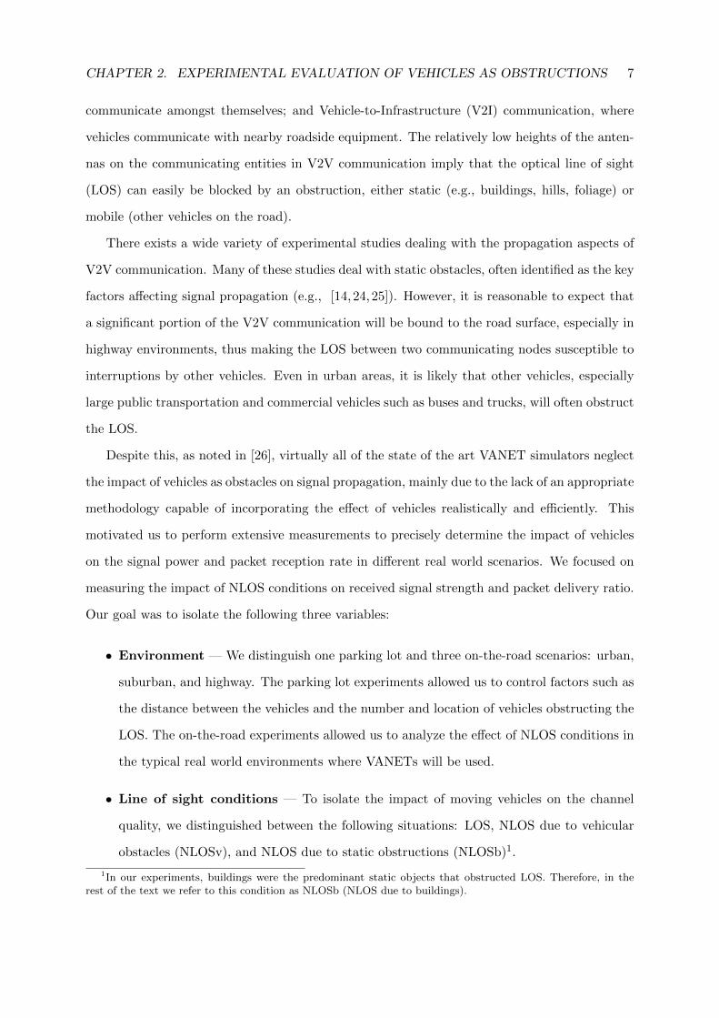
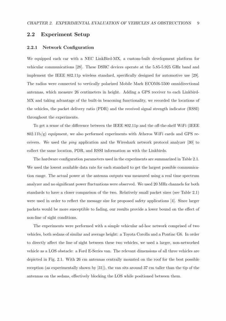
2.1 Hardware configuration parameters . . . . . . . . . . . . . . . . . . . . . . . . . . 8
3.1 Analyzed highway datasets . . . . . . . . . . . . . . . . . . . . . . . . . . . . . . 33
3.2 Parameters of the Best Fit Distributions for Vehicle Speed and Inter-vehicle spacing 34
3.3 Parameters of the Best Fit Distributions for Vehicle Width and Height . . . . . . 35
3.4 P (LOS) for A3 and A28 . . . . . . . . . . . . . . . . . . . . . . . . . . . . . . . . 37
3.5 Variation of P (LOS)i over time for the observed range of 750 m on A28. . . . . . 39
3.6 Requirements for DSRC Receiver Performance . . . . . . . . . . . . . . . . . . . 41
3.7 Dimensions of Vehicles . . . . . . . . . . . . . . . . . . . . . . . . . . . . . . . . . 42
4.1 Porto Downtown Buildings and Vehicle Dataset . . . . . . . . . . . . . . . . . . . 50
4.2 Dimensions of Vehicles Used in the Experiments . . . . . . . . . . . . . . . . . . 50
4.3 Modeling different link types . . . . . . . . . . . . . . . . . . . . . . . . . . . . . 57
4.4 Minimum and fading σ extracted from experimental data . . . . . . . . . . . . . 69
4.5 Max. communication ranges used for different link types . . . . . . . . . . . . . . 73
5.1 Aerial photography dataset (A28 highway) . . . . . . . . . . . . . . . . . . . . . . 92
5.2 Dimensions of Vehicles Used in the Experiments . . . . . . . . . . . . . . . . . . 94
5.3 Percentage of Vehicles Used for Relaying . . . . . . . . . . . . . . . . . . . . . . . 113
xvi
Chapter 1
Introduction
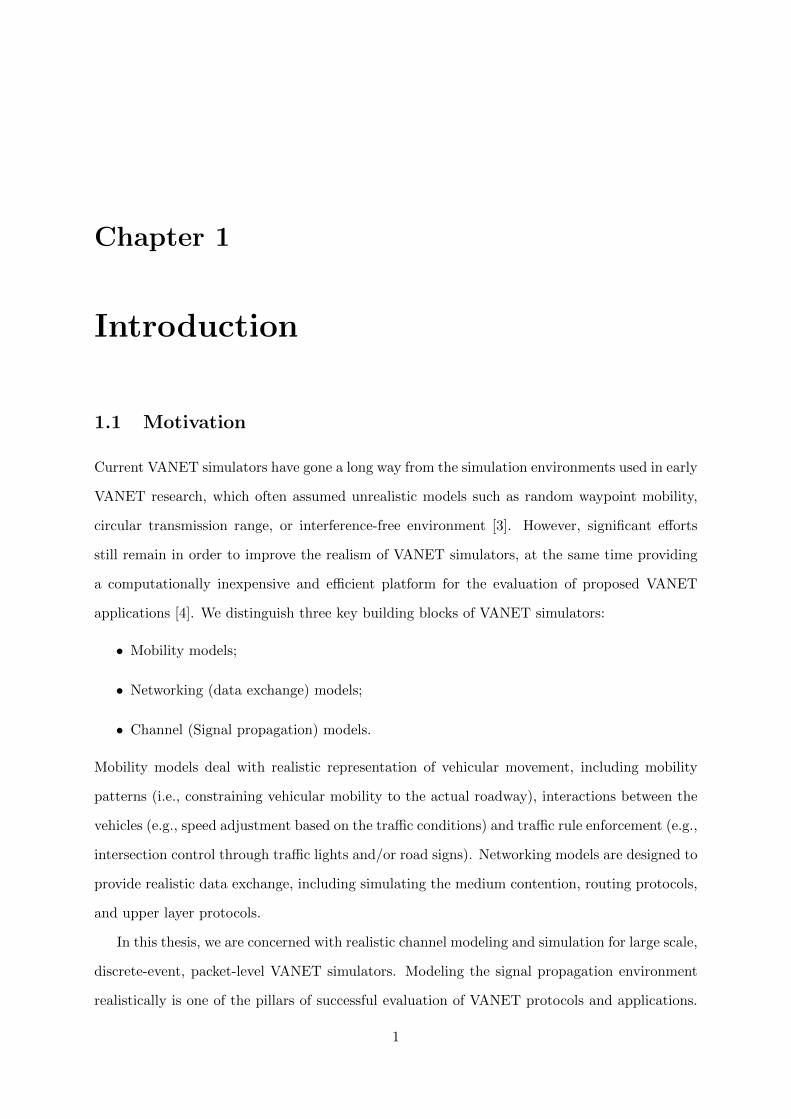
1.1 Motivation
Current VANET simulators have gone a long way from the simulation environments used in early
VANET research, which often assumed unrealistic models such as random waypoint mobility,
circular transmission range, or interference-free environment [3]. However, significant efforts
still remain in order to improve the realism of VANET simulators, at the same time providing
a computationally inexpensive and efficient platform for the evaluation of proposed VANET
applications [4]. We distinguish three key building blocks of VANET simulators:
• Mobility models;
• Networking (data exchange) models;
• Channel (Signal propagation) models.
Mobility models deal with realistic representation of vehicular movement, including mobility
patterns (i.e., constraining vehicular mobility to the actual roadway), interactions between the
vehicles (e.g., speed adjustment based on the traffic conditions) and traffic rule enforcement (e.g.,
intersection control through traffic lights and/or road signs). Networking models are designed to
provide realistic data exchange, including simulating the medium contention, routing protocols,
and upper layer protocols.
In this thesis, we are concerned with realistic channel modeling and simulation for large scale,
discrete-event, packet-level VANET simulators. Modeling the signal propagation environment
realistically is one of the pillars of successful evaluation of VANET protocols and applications.
1
CHAPTER 1. INTRODUCTION 2
Channel Modeling
Large Scale (Macroscopic)
Medium Scale (Mesoscopic)
Small Scale (Microscopic)
Level of Detail
Non-Geometrical Stochastic
Geometrical Stochastic
Environment Modeling
Geometrical Deterministic
Mobile Static
Object Types
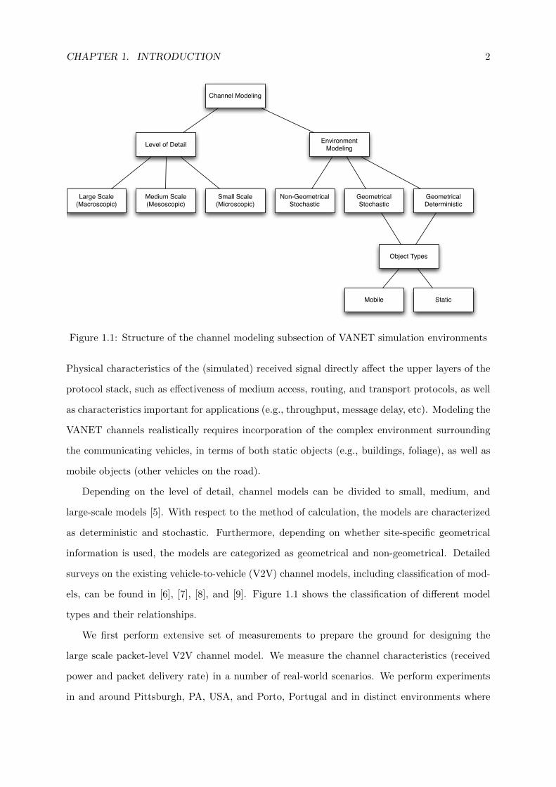
Figure 1.1: Structure of the channel modeling subsection of VANET simulation environments
Physical characteristics of the (simulated) received signal directly affect the upper layers of the
protocol stack, such as effectiveness of medium access, routing, and transport protocols, as well
as characteristics important for applications (e.g., throughput, message delay, etc). Modeling the
VANET channels realistically requires incorporation of the complex environment surrounding
the communicating vehicles, in terms of both static objects (e.g., buildings, foliage), as well as
mobile objects (other vehicles on the road).
Depending on the level of detail, channel models can be divided to small, medium, and
large-scale models [5]. With respect to the method of calculation, the models are characterized
as deterministic and stochastic. Furthermore, depending on whether site-specific geometrical
information is used, the models are categorized as geometrical and non-geometrical. Detailed
surveys on the existing vehicle-to-vehicle (V2V) channel models, including classification of mod-
els, can be found in [6], [7], [8], and [9]. Figure 1.1 shows the classification of different model
types and their relationships.
We first perform extensive set of measurements to prepare the ground for designing the
large scale packet-level V2V channel model. We measure the channel characteristics (received
power and packet delivery rate) in a number of real-world scenarios. We perform experiments
in and around Pittsburgh, PA, USA, and Porto, Portugal and in distinct environments where
CHAPTER 1. INTRODUCTION 3
VANETs will be deployed: highway, suburban, urban, open space, and isolated parking lot.
We characterize the impact of both mobile objects (vehicles) and static objects (buildings and
foliage) on the received power, packet delivery rate, and effective range.
Based on the measurements, in the second part of the thesis we design a computationally
efficient packet-level V2V channel model for simulating vehicular communications in discrete-
event simulators. We first describe existing channel models implemented in large scale packet-
level VANET simulators and motivate the need for more accurate models that are able to
capture the behavior of the signal on a per-link basis, rather than relying solely on the overall
statistical properties of the environment. More specifically, as shown in [1] and [2]), simplified
stochastic radio models (e.g., free space [10], log-distance path loss [11], etc.), which are based
on the statistical properties of the chosen environment and do not account for the specific
obstacles in the region of interest, are unable to provide satisfactory accuracy for typical VANET
scenarios. Contrary to this, topography-specific, highly realistic channel models (e.g., based on
ray-tracing [12]) yield results that are in very good agreement with the real world. However,
these models are: 1) computationally too expensive due to prohibitive computation costs as the
network grows; and 2) most often bound to a specific location for which a detailed geographic
database is required, thus making them impractical for extensive simulation studies. For these
reasons, such models have not been implemented in VANET simulators. We explore how site-
specific models can be used so that both of these caveats are minimized, at the same time
retaining the realism of the model.
With regards to Fig. 1.1, we propose a model that can be considered a hybrid between
geometrical stochastic and geometrical deterministic models. It models the path loss determin-
istically using the geographical descriptors of the objects (namely, object outlines). Additionally,
based on the location and the number of objects, the model stochastically assigns the additional
signal variation (fading) on top of the path loss. The model takes into account both mobile and
static objects.
The model leverages a limited amount of geographical information that is easily available in
order to produce results comparable to those in the real world. Specifically, we use locations of
the vehicles along with the information on the location and shape of the buildings and foliage.
Vehicle locations are available through either real world traces (e.g., via GPS) or traffic mobility
models, whereas the building and foliage outlines and locations are available freely from projects
CHAPTER 1. INTRODUCTION 4
such as the OpenStreetMap (www.openstreetmap.org). The premise of the model is that line of
sight (LOS) and non-LOS (NLOS) links exhibit considerably different channel characteristics.
This is corroborated by numerous studies, both experimental and analytical (e.g., [13], [14],
[15], [16], and [17]), which have shown that the resulting channel characteristics for LOS and
non-LOS links are fundamentally different. For this reason, our approach to modeling is to
use simple geographical descriptors of the simulated environment (outlines of buildings, foliage,
and vehicles on the road) to determine the large-scale signal shadowing effects and classify the
communication links into three groups:
• Line of sight (LOS) – links that have an unobstructed optical path between the transmit-
ting and receiving antennas;
• Non-LOS due to vehicles (NLOSv) – links whose LOS is obstructed by other vehicles;
• Non-LOS due to buildings/foliage (NLOSb) – links whose LOS is obstructed by static
objects (buildings or foliage).
We take a specific approach in estimating the properties for each of these link types. The model is
intended for implementation in packet-level, discrete-event VANET simulators (notable examples
are Jist/SWANS [18], NS-2 [19], NS-3 [20], QualNet [21], etc.). We employ computational
geometry concepts suitable for representation of the geographic data required in simulating
VANETs. We form a bounding volume hierarchy (BVH) structures [22], in which we store
the information about outlines of both the vehicles and buildings. VANET-related geometric
data lends itself to an efficient BVH implementation, due to its inherent geometrical structure
(namely, relatively simple object outlines and no overlapping of building and vehicle outlines).
The model can be used with any discrete-event VANET simulator, provided that: a) location of
vehicles are known (which is a must for VANET simulations); and b) location and the outlines of
buildings and streets are known (this information is freely available from numerous geographical
databases).
In the final part of the thesis, we discuss an application is aimed at alleviating the impact of
vehicular obstructions by selecting the tall vehicles as relaying nodes. We evaluate this applica-
tion using the model we introduced. Specifically, we show that, using small-scale experiments,
significant benefits can be obtained by opting for tall vehicles as next hop relays, as opposed
CHAPTER 1. INTRODUCTION 5
to short (personal) vehicles. We perform simulations with the proposed model and we validate
the results with experiments involving tall and short vehicles. The proposed technique matches
the existing techniques in low vehicle density scenarios and outperforms them in high density
scenarios.
1.2 Thesis Organization
The rest of the thesis is organized as follows. In Chapter 2, we present a set of measurements
which provide insights into the impact of vehicular obstructions on inter-vehicle communication.
Based on the insights of the measurement study, Chapter 3 presents a model that incorporates
the vehicles as three-dimensional objects in the channel modeling. The model takes into account
the impact of vehicles on the line of sight obstruction, received signal power, packet reception
rate, and message reachability. In order to enable realistic channel simulation in urban areas for
VANET simulators, in Chapter 4 we introduce a channel model that incorporates both vehicles
and static objects (namely, buildings and foliage). Furthermore, in Chapter 5 we perform
experiments to determine how much of the adverse effects of vehicular obstructions can be
alleviated using the tall vehicles’ raised antennas to achieve a better channel. Based on the
measurements, we develop a relaying technique that utilizes tall vehicles to improve effective
communication range and packet delivery. Finally, concluding remarks and future research
directions are given in Chapter 6.
Chapter 2
Experimental Evaluation of Vehicles
as Obstructions
Channel models for vehicular networks typically disregard the effect of vehicles as physical
obstructions for the wireless signal. We tested the validity of this simplification by quantifying
the impact of obstructions through a series of wireless experiments reported in [16]. Using two
cars equipped with Dedicated Short Range Communications (DSRC) hardware [23] designed for
vehicular use, we perform experimental measurements in order to collect received signal power
and packet delivery ratio information in a multitude of relevant scenarios: parking lot, highway,
suburban and urban canyon. Upon separating the data into line of sight (LOS) and non-line of
sight (NLOS) categories, our results show that obstructing vehicles cause significant impact on
the channel quality. A single obstacle can cause a drop of over 20 dB in received signal strength
when two cars communicate at a distance of 10 m. At longer distances, NLOS conditions affect
the usable communication range, effectively halving the distance at which communication can
be achieved with 90% chance of success. The presented results motivate the inclusion of vehicles
in the radio propagation models used for VANET simulation in order to increase the level of
realism.
2.1 Motivation
Based on the parties involved, two main communication paradigms exist in Vehicular Ad Hoc
Networks (VANETs): Vehicle-to-Vehicle (V2V) communication, where vehicles on the road
6
CHAPTER 2. EXPERIMENTAL EVALUATION OF VEHICLES AS OBSTRUCTIONS 7
communicate amongst themselves; and Vehicle-to-Infrastructure (V2I) communication, where
vehicles communicate with nearby roadside equipment. The relatively low heights of the anten-
nas on the communicating entities in V2V communication imply that the optical line of sight
(LOS) can easily be blocked by an obstruction, either static (e.g., buildings, hills, foliage) or
mobile (other vehicles on the road).
There exists a wide variety of experimental studies dealing with the propagation aspects of
V2V communication. Many of these studies deal with static obstacles, often identified as the key
factors affecting signal propagation (e.g., [14, 24, 25]). However, it is reasonable to expect that
a significant portion of the V2V communication will be bound to the road surface, especially in
highway environments, thus making the LOS between two communicating nodes susceptible to
interruptions by other vehicles. Even in urban areas, it is likely that other vehicles, especially
large public transportation and commercial vehicles such as buses and trucks, will often obstruct
the LOS.
Despite this, as noted in [26], virtually all of the state of the art VANET simulators neglect
the impact of vehicles as obstacles on signal propagation, mainly due to the lack of an appropriate
methodology capable of incorporating the effect of vehicles realistically and efficiently. This
motivated us to perform extensive measurements to precisely determine the impact of vehicles
on the signal power and packet reception rate in different real world scenarios. We focused on
measuring the impact of NLOS conditions on received signal strength and packet delivery ratio.
Our goal was to isolate the following three variables:
• Environment — We distinguish one parking lot and three on-the-road scenarios: urban,
suburban, and highway. The parking lot experiments allowed us to control factors such as
the distance between the vehicles and the number and location of vehicles obstructing the
LOS. The on-the-road experiments allowed us to analyze the effect of NLOS conditions in
the typical real world environments where VANETs will be used.
• Line of sight conditions — To isolate the impact of moving vehicles on the channel
quality, we distinguished between the following situations: LOS, NLOS due to vehicular
obstacles (NLOSv), and NLOS due to static obstructions (NLOSb)1.
1In our experiments, buildings were the predominant static objects that obstructed LOS. Therefore, in therest of the text we refer to this condition as NLOSb (NLOS due to buildings).
CHAPTER 2. EXPERIMENTAL EVALUATION OF VEHICLES AS OBSTRUCTIONS 8
1450
mm
208
5 m
m
1466
mm
4539 mm 5504 mm 4801 mm
Figure 2.1: Scaled drawing of the vehicles used in the experiments. Left to right: 2009Toyota Corolla, a 2010 Ford E-Series, and a 2009 Pontiac G6. Blueprints courtesy of car-blueprints.info [27].
Parameter 802.11p 802.11b/g
Channel 180 1
Center frequency (MHz) 5900 2412
Bandwidth (MHz) 20 20
Data rate (Mbps) 6 1
Tx power (setting, dBm) 18 18
Tx power (measured, dBm) 10 16
Antenna gain (dBi) 5 3
Beacon frequency (Hz) 10 10
Beacon size (Byte) 36 64
Table 2.1: Hardware configuration parameters
• Time of day — We introduce this variable to help determine how often the vehicles en-
counter NLOSv conditions at different times of day (since NLOSv obstruction is temporally
variable) and how this affects the signal.
Using these variables and following the work reported in [15], we designed a set of experiments
using two vehicles equipped with Dedicated Short Range Communication (DSRC) devices to
characterize the impact of vehicles as obstacles on V2V communication at the communication
link level. We aimed at quantifying the additional attenuation and packet loss due to vehicular
obstructions.
The rest of the chapter is organized as follows. The experimental setup is described in
Section 2.2. Section 3.5 discusses the results and Section 5.5 describes previous work on exper-
imental evaluation and modeling of V2V communication. Section 3.6 concludes the chapter.
CHAPTER 2. EXPERIMENTAL EVALUATION OF VEHICLES AS OBSTRUCTIONS 9
2.2 Experiment Setup
2.2.1 Network Configuration
We equipped each car with a NEC LinkBird-MX, a custom-built development platform for
vehicular communications [28]. These DSRC devices operate at the 5.85-5.925 GHz band and
implement the IEEE 802.11p wireless standard, specifically designed for automotive use [29].
The radios were connected to vertically polarized Mobile Mark ECOM6-5500 omnidirectional
antennas, which measure 26 centimeters in height. Adding a GPS receiver to each Linkbird-
MX and taking advantage of the built-in beaconing functionality, we recorded the locations of
the vehicles, the packet delivery ratio (PDR) and the received signal strength indicator (RSSI)
throughout the experiments.
To get a sense of the difference between the IEEE 802.11p and the off-the-shelf WiFi (IEEE
802.11b/g) equipment, we also performed experiments with Atheros WiFi cards and GPS re-
ceivers. We used the ping application and the Wireshark network protocol analyzer [30] to
collect the same location, PDR, and RSSI information as with the Linkbirds.
The hardware configuration parameters used in the experiments are summarized in Table 2.1.
We used the lowest available data rate for each standard to get the largest possible communica-
tion range. The actual power at the antenna outputs was measured using a real time spectrum
analyzer and no significant power fluctuations were observed. We used 20 MHz channels for both
standards to have a closer comparison of the two. Relatively small packet sizes (see Table 2.1)
were used in order to reflect the message size for proposed safety applications [4]. Since larger
packets would be more susceptible to fading, our results provide a lower bound on the effect of
non-line of sight conditions.
The experiments were performed with a simple vehicular ad-hoc network comprised of two
vehicles, both sedans of similar and average height: a Toyota Corolla and a Pontiac G6. In order
to directly affect the line of sight between these two vehicles, we used a larger, non-networked
vehicle as a LOS obstacle: a Ford E-Series van. The relevant dimensions of all three vehicles are
depicted in Fig. 2.1. With 26 cm antennas centrally mounted on the roof for the best possible
reception (as experimentally shown by [31]), the van sits around 37 cm taller than the tip of the
antennas on the sedans, effectively blocking the LOS while positioned between them.
CHAPTER 2. EXPERIMENTAL EVALUATION OF VEHICLES AS OBSTRUCTIONS 10
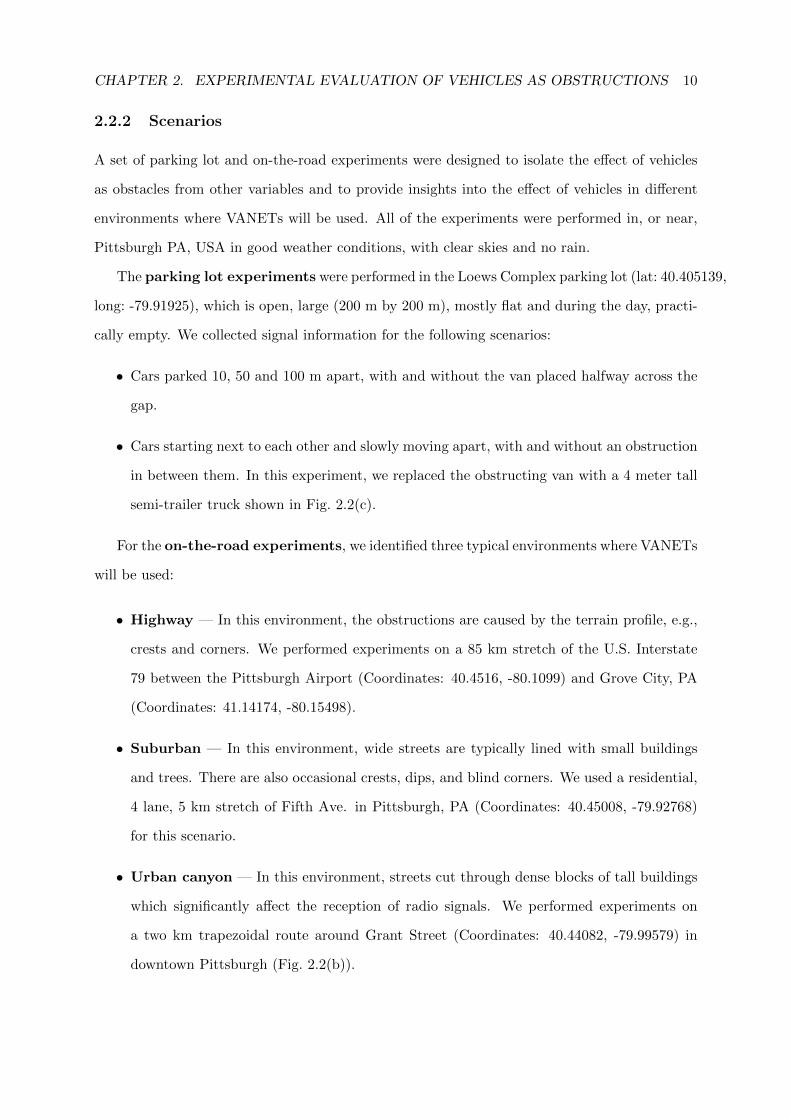
2.2.2 Scenarios
A set of parking lot and on-the-road experiments were designed to isolate the effect of vehicles
as obstacles from other variables and to provide insights into the effect of vehicles in different
environments where VANETs will be used. All of the experiments were performed in, or near,
Pittsburgh PA, USA in good weather conditions, with clear skies and no rain.
The parking lot experiments were performed in the Loews Complex parking lot (lat: 40.405139,
long: -79.91925), which is open, large (200 m by 200 m), mostly flat and during the day, practi-
cally empty. We collected signal information for the following scenarios:
• Cars parked 10, 50 and 100 m apart, with and without the van placed halfway across the
gap.
• Cars starting next to each other and slowly moving apart, with and without an obstruction
in between them. In this experiment, we replaced the obstructing van with a 4 meter tall
semi-trailer truck shown in Fig. 2.2(c).
For the on-the-road experiments, we identified three typical environments where VANETs
will be used:
• Highway — In this environment, the obstructions are caused by the terrain profile, e.g.,
crests and corners. We performed experiments on a 85 km stretch of the U.S. Interstate
79 between the Pittsburgh Airport (Coordinates: 40.4516, -80.1099) and Grove City, PA
(Coordinates: 41.14174, -80.15498).
• Suburban — In this environment, wide streets are typically lined with small buildings
and trees. There are also occasional crests, dips, and blind corners. We used a residential,
4 lane, 5 km stretch of Fifth Ave. in Pittsburgh, PA (Coordinates: 40.45008, -79.92768)
for this scenario.
• Urban canyon — In this environment, streets cut through dense blocks of tall buildings
which significantly affect the reception of radio signals. We performed experiments on
a two km trapezoidal route around Grant Street (Coordinates: 40.44082, -79.99579) in
downtown Pittsburgh (Fig. 2.2(b)).
CHAPTER 2. EXPERIMENTAL EVALUATION OF VEHICLES AS OBSTRUCTIONS 11
For each environment, we performed the experiments by driving the cars for approximately
one hour, all the time collecting GPS and received signal information. Throughout the ex-
periment, we videotaped the view from the car following in the back for later analysis of the
LOS/NLOSv/NLOSb conditions.
We performed two one-hour experiment runs for each on-the-road scenario: one at a rush
hour period with frequent NLOSv conditions, and the other late at night, when the number of
vehicles on the road (and consequently, the frequency of vehicle-induced – NLOSv – conditions)
is substantially lower. This, by itself, worked as a heuristic for the LOS conditions. Furthermore,
to more accurately distinguish between LOS conditions, we used the recorded videos to separate
the LOS, NLOSv, and NLOSb data.
2.3 Results
2.3.1 Parking lot experiments
All of the parking lot experiments were performed at relatively short distances, meaning the
packet delivery ratio was almost always 100%. We therefore focus on RSSI to analyze the effect
of LOS conditions on channel quality. For ease of presentation, we report the RSSI values in dB
as provided by the Atheros cards. The RSSI values can be converted to dBm by subtracting 95
from the presented values.
First, we consider the experiments where the cars were placed at a fixed distance from each
other. Figure 2.3 shows the RSSI results. The standard deviation was under 1 dB and the
95% confidence intervals were too small to represent; we thus focus on the average values. The
difference in absolute RSSI values between the 802.11b/g and 802.11p standards is mainly due
to the difference in antenna gains, hardware calibrations, and the quality of the radios.
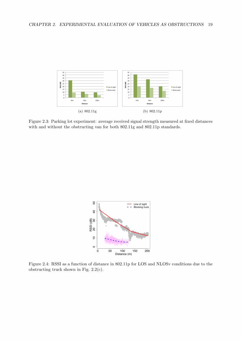
Blocking the LOS has clear negative effects on the RSSI. Even though the absolute values
differ between the standards, the overall impact of NLOSv conditions is quite similar. At 10 m,
the van reduced the RSSI by approximately 20 dB in both cases. As the distance between
communicating nodes increased, the effect of the van was gradually reduced. At 100 m, the
RSSI in the NLOSv case was approximately 5 and 7 dB below the LOS case for 802.11b/g and
802.11p, respectively.
Furthermore, we performed an experiment where, starting with the cars next to each other,
CHAPTER 2. EXPERIMENTAL EVALUATION OF VEHICLES AS OBSTRUCTIONS 12
we slowly moved them apart. We did this experiment without any LOS obstruction and with
a 4 m tall semi-trailer truck parked halfway between the vehicles (Fig. 2.2(c)). Figure 2.4
shows the RSSI as a function of distance. The dots represent individual samples, while the
curves show the result of applying locally weighted scatter plot smoothing (LOWESS) to the
individual points. The truck had a large impact on RSSI, with a loss of approximately 27 dB at
the smallest recorded distance of 26 m (the length of the truck) when compared with the LOS
case. For comparison, the van attenuated the signal by 12 dB at 20 m. The RSSI drop caused
by the truck decreased as the cars move further away from it, an indication that the angle of
the antennas’ field of view that gets blocked makes a difference.
2.3.2 On-the-road experiments
For the on-the-road experiments, we drove the test vehicles in the three scenarios identified in
Section 2.2.2 and collected RSSI and PDR information to use as indicators of channel quality.
To accurately analyze the LOS and NLOS conditions, we placed each data point in one of
the following categories, according to the information we obtained by reviewing the experiment
videos:
• Line of sight (LOS) — no obstacles between the sender and receiver vehicles.
• Vehicular obstructions (NLOSv) — LOS blocked by other vehicles on the road.
• Static obstructions (NLOSb) — LOS blocked by immovable objects, such as buildings
or terrain features, like crests and hills.
To compute the PDR, we counted the number of beacons sent by the sender and the number
of beacons received at the receiver in a given time interval. We used a granularity of 5 seconds
(50 beacons) for the calculations. We use 10 m bins for the distance and show: the mean, its
associated 95% confidence intervals and the 20 and 80% quantiles (dashed lines). To make the
data easier to read, we use LOWESS to smooth the curves.
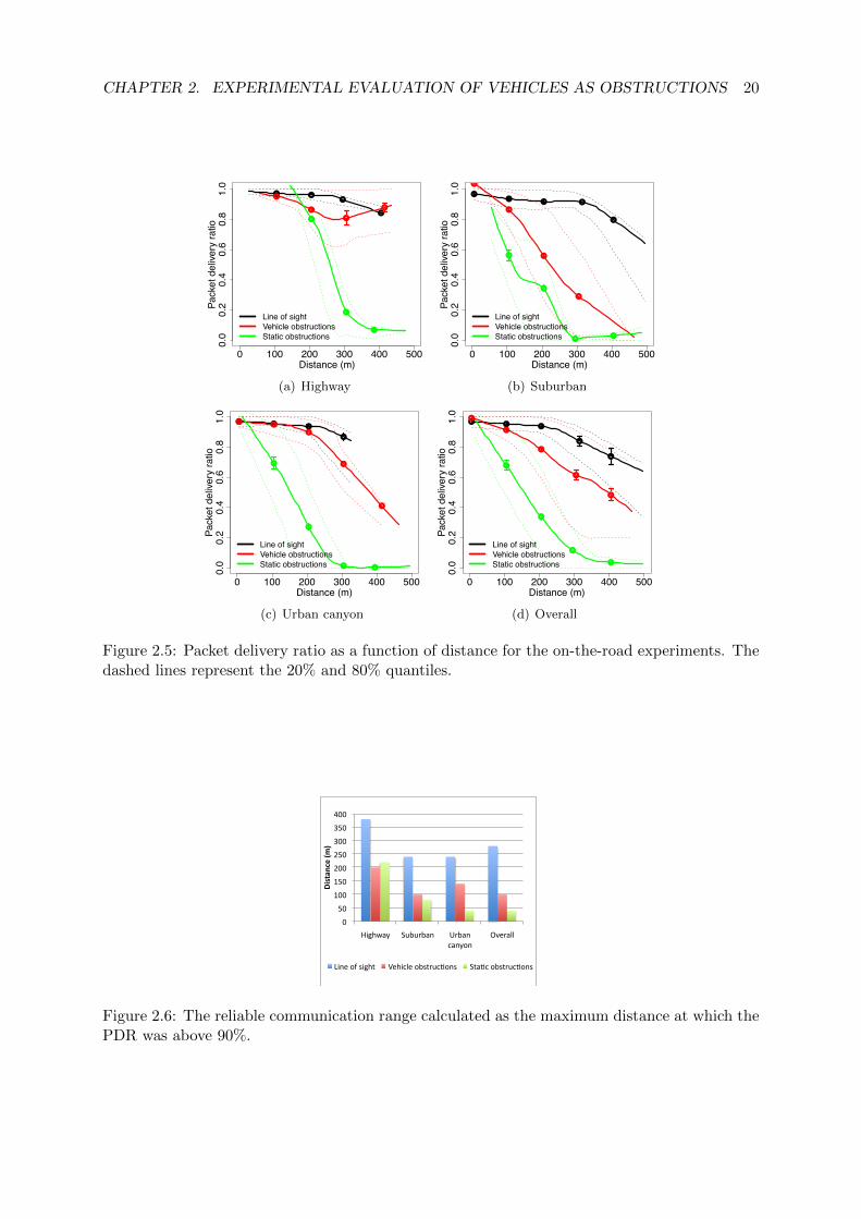
Figure 2.5 shows the PDR as a function of distance separately for each on-the-road scenario,
as well as aggregated over all three. For all scenarios, the PDR for the LOS case is above 80%
even at long distances, only dropping below that threshold in the suburban scenario and only
after 400 m. At short distances, the difference between the PDR for LOS and NLOSv is almost
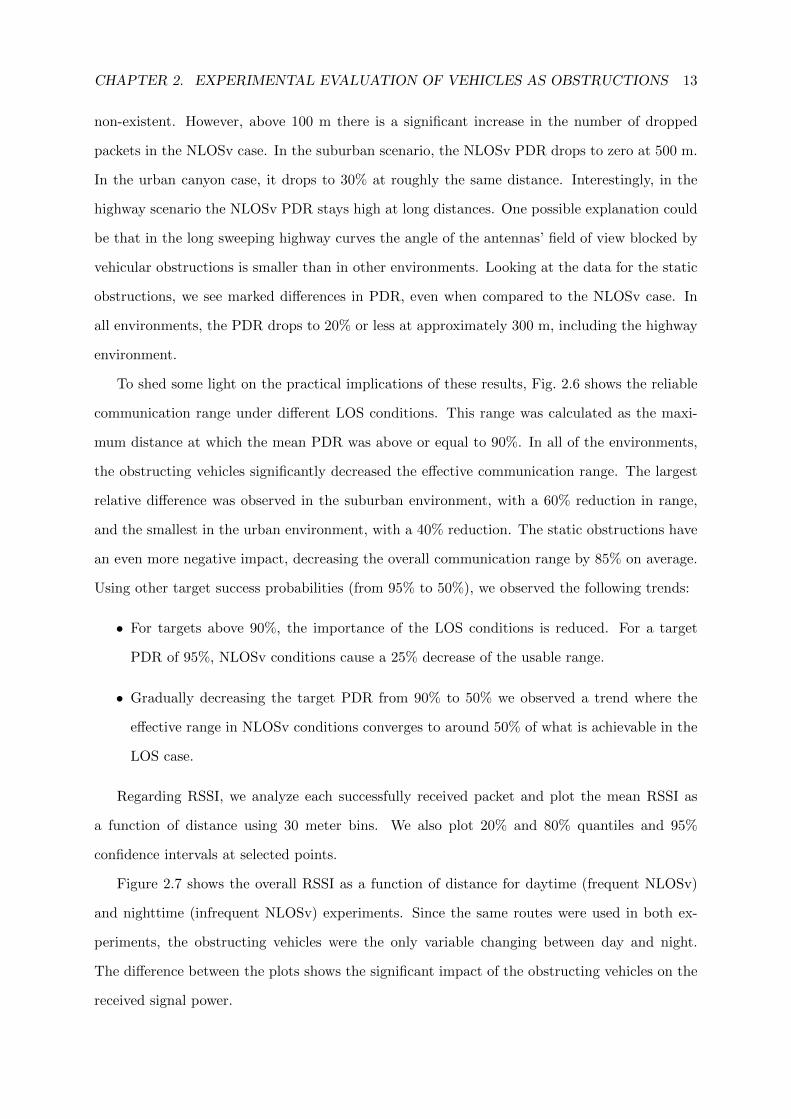
CHAPTER 2. EXPERIMENTAL EVALUATION OF VEHICLES AS OBSTRUCTIONS 13
non-existent. However, above 100 m there is a significant increase in the number of dropped
packets in the NLOSv case. In the suburban scenario, the NLOSv PDR drops to zero at 500 m.
In the urban canyon case, it drops to 30% at roughly the same distance. Interestingly, in the
highway scenario the NLOSv PDR stays high at long distances. One possible explanation could
be that in the long sweeping highway curves the angle of the antennas’ field of view blocked by
vehicular obstructions is smaller than in other environments. Looking at the data for the static
obstructions, we see marked differences in PDR, even when compared to the NLOSv case. In
all environments, the PDR drops to 20% or less at approximately 300 m, including the highway
environment.
To shed some light on the practical implications of these results, Fig. 2.6 shows the reliable
communication range under different LOS conditions. This range was calculated as the maxi-
mum distance at which the mean PDR was above or equal to 90%. In all of the environments,
the obstructing vehicles significantly decreased the effective communication range. The largest
relative difference was observed in the suburban environment, with a 60% reduction in range,
and the smallest in the urban environment, with a 40% reduction. The static obstructions have
an even more negative impact, decreasing the overall communication range by 85% on average.
Using other target success probabilities (from 95% to 50%), we observed the following trends:
• For targets above 90%, the importance of the LOS conditions is reduced. For a target
PDR of 95%, NLOSv conditions cause a 25% decrease of the usable range.
• Gradually decreasing the target PDR from 90% to 50% we observed a trend where the
effective range in NLOSv conditions converges to around 50% of what is achievable in the
LOS case.
Regarding RSSI, we analyze each successfully received packet and plot the mean RSSI as
a function of distance using 30 meter bins. We also plot 20% and 80% quantiles and 95%
confidence intervals at selected points.
Figure 2.7 shows the overall RSSI as a function of distance for daytime (frequent NLOSv)
and nighttime (infrequent NLOSv) experiments. Since the same routes were used in both ex-
periments, the obstructing vehicles were the only variable changing between day and night.
The difference between the plots shows the significant impact of the obstructing vehicles on the
received signal power.
CHAPTER 2. EXPERIMENTAL EVALUATION OF VEHICLES AS OBSTRUCTIONS 14
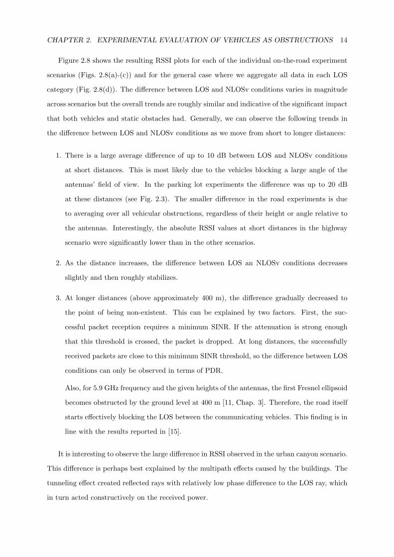
Figure 2.8 shows the resulting RSSI plots for each of the individual on-the-road experiment
scenarios (Figs. 2.8(a)-(c)) and for the general case where we aggregate all data in each LOS
category (Fig. 2.8(d)). The difference between LOS and NLOSv conditions varies in magnitude
across scenarios but the overall trends are roughly similar and indicative of the significant impact
that both vehicles and static obstacles had. Generally, we can observe the following trends in
the difference between LOS and NLOSv conditions as we move from short to longer distances:
1. There is a large average difference of up to 10 dB between LOS and NLOSv conditions
at short distances. This is most likely due to the vehicles blocking a large angle of the
antennas’ field of view. In the parking lot experiments the difference was up to 20 dB
at these distances (see Fig. 2.3). The smaller difference in the road experiments is due
to averaging over all vehicular obstructions, regardless of their height or angle relative to
the antennas. Interestingly, the absolute RSSI values at short distances in the highway
scenario were significantly lower than in the other scenarios.
2. As the distance increases, the difference between LOS an NLOSv conditions decreases
slightly and then roughly stabilizes.
3. At longer distances (above approximately 400 m), the difference gradually decreased to
the point of being non-existent. This can be explained by two factors. First, the suc-
cessful packet reception requires a minimum SINR. If the attenuation is strong enough
that this threshold is crossed, the packet is dropped. At long distances, the successfully
received packets are close to this minimum SINR threshold, so the difference between LOS
conditions can only be observed in terms of PDR.
Also, for 5.9 GHz frequency and the given heights of the antennas, the first Fresnel ellipsoid
becomes obstructed by the ground level at 400 m [11, Chap. 3]. Therefore, the road itself
starts effectively blocking the LOS between the communicating vehicles. This finding is in
line with the results reported in [15].
It is interesting to observe the large difference in RSSI observed in the urban canyon scenario.
This difference is perhaps best explained by the multipath effects caused by the buildings. The
tunneling effect created reflected rays with relatively low phase difference to the LOS ray, which
in turn acted constructively on the received power.
CHAPTER 2. EXPERIMENTAL EVALUATION OF VEHICLES AS OBSTRUCTIONS 15
We also captured data pertaining to the effect of static obstructions on the channel quality.
In the urban canyon the obstructions were mainly buildings, which had a profound impact on
RSSI. A loss of around 15 dB compared with the NLOSv case at shorter distances and around
4 dB at larger distances was observed. In the suburban and highway scenarios, obstructions
were mostly created by crests on the road. The results indicate that they can make a difference
of up to 3 dB of additional attenuation atop the NLOSv attenuation.
The results presented in this section inevitably point to the fact that obstructing vehicles
have to be accounted for in channel modeling. Not modeling the vehicles results in overly
optimistic received signal power, PDR and communication range.
2.4 Related Work
Regarding V2V communication, Otto et al. in [14] performed V2V experiments in the 2.4 GHz
frequency band in an open road environment and reported a significantly worse signal reception
during a traffic heavy, rush hour period in comparison to a no traffic, late night period. A similar
study presented in [32] analyzed the signal propagation in “crowded” and “uncrowded” highway
scenarios (based on the number of vehicles on the road) for the 60 GHz frequency band, and
reported significantly higher path loss for the crowded scenarios.
With regards to experimental evaluation of the impact of vehicles and their incorporation
in channel models, a lightweight model based on Markov chains was proposed in [1]. Based on
experimental measurements, the model extends the stochastic shadowing model and aims at cap-
turing the time-varying nature of the V2V channel based on a set of predetermined parameters
describing the environment. Tan et al. in [33] performed experimental measurements in various
environments (urban, rural, highway) at 5.9 GHz to determine the suitability of DSRC for vehic-
ular environments with respect to delay spread and Doppler shift. The paper distinguishes LOS
and NLOS communication scenarios by coarsely dividing the overall obstruction levels. The
results showed that DSRC provides satisfactory performance of the delay spread and Doppler
shift, provided that the message is below a certain size. A similar study was reported in [34],
where experiments were performed at 5.2 GHz. Path loss, power delay profile, and Doppler
shift were analyzed and statistical parameters, such as path loss exponent, were deduced for
given environments. Based on measurements, a realistic model based on optical ray-tracing was
CHAPTER 2. EXPERIMENTAL EVALUATION OF VEHICLES AS OBSTRUCTIONS 16
presented in [12]. The model encompassed all of the obstructions in a given area, including the
vehicles, and yielded results comparable with the real world measurements. However, the high
realism that the model exhibits is achieved at the expense of high computational complexity.
Experiments in urban, suburban, and highway environments with two levels of traffic density
(high and low) were reported in [35]. The results showed significantly differing channel properties
in low and high traffic scenarios. Based on the measurements, several V2V channel models were
proposed. The presented models are specific for a given environment and vehicle traffic density.
Several other studies [13, 36–38] point out that other vehicles apart from the transmitter and
receiver could be an important factor in modeling the signal propagation by obstructing the
LOS between the communicating vehicles.
Virtually all of the studies mentioned above emphasize that LOS and NLOS for V2V com-
munication have to be modeled differently, and that vehicles act as obstacles and affect signal
propagation to some extent. However, these studies at most quantify the macroscopic impact
of the vehicles by defining V2V communication environments as uncrowded (LOS) or crowded
(NLOS), depending on the relative vehicle density, without analyzing the impact that obstruct-
ing vehicles have on a single communication link.
2.5 Conclusions
In this work we set out to experimentally evaluate the impact of obstructing vehicles on V2V
communication. For this purpose, we ran a set of experiments with near-production 802.11p
hardware in a multitude of relevant scenarios: parking lot, highway, suburban and urban canyon.
Our results indicate that vehicles blocking the line of sight significantly attenuate the signal
when compared to line of sight conditions across all scenarios. Also, the effect appears to be
more pronounced the closer the obstruction is to the sender, with over 20 dB attenuation at
bumper-to-bumper distances. The additional attenuation decreased the packet delivery ratio at
longer distances, halving the effective communication range for target average packet delivery
ratios between 90% and 50%. The effect of static obstacles such as buildings and hills was also
analyzed and shown to be even more pronounced than that of vehicular obstructions.
With respect to channel modeling, even the experimental measurements proposed for certi-
fication testing of DSRC equipment [39] do not directly address the effect of vehicles in the V2V

CHAPTER 2. EXPERIMENTAL EVALUATION OF VEHICLES AS OBSTRUCTIONS 17
environment, thus potentially underestimating the attenuation and packet loss. Our work shows
that not modeling vehicles as physical obstructions takes away from the realism of the channel
models, thus affecting the simulation of both the physical layer and the upper layer protocols.
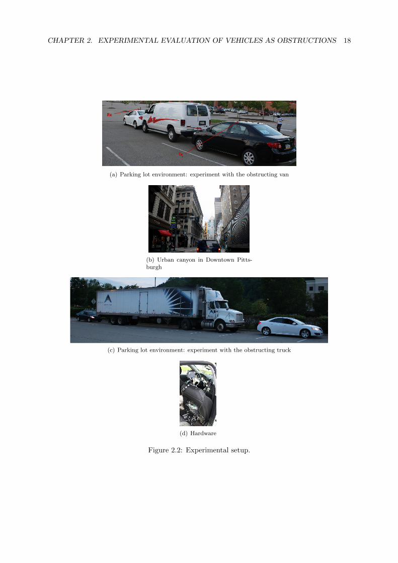
CHAPTER 2. EXPERIMENTAL EVALUATION OF VEHICLES AS OBSTRUCTIONS 18
RxRx
Tx
(a) Parking lot environment: experiment with the obstructing van
(b) Urban canyon in Downtown Pitts-burgh
(c) Parking lot environment: experiment with the obstructing truck
(d) Hardware
Figure 2.2: Experimental setup.
CHAPTER 2. EXPERIMENTAL EVALUATION OF VEHICLES AS OBSTRUCTIONS 19
0
5
10
15
20
25
30
35
40
45
10m 50m 100m
RSSI(d
B)
Distance
Lineofsight
Obstructed
(a) 802.11g
0
5
10
15
20
25
30
35
40
45
10m 50m 100m
RSSI(d
B)
Distance
Lineofsight
Obstructed
(b) 802.11p
Figure 2.3: Parking lot experiment: average received signal strength measured at fixed distanceswith and without the obstructing van for both 802.11g and 802.11p standards.
●●●●●●●●●●●●●●●●●●●●●●●●
●●●●●●●●●●●●●●●●●
●●●●●●
●●●●●●●●●●●●●●●●●
●●●●●●●●●●●●●●
●●●●●●●●●●●●●●●
●●●●●●●●●●●
●
●
●
●
●●●
●
●
●●●●
●
●●●●●●●●●●●●
●
●●●●●●
●
●●
●
●
●
●●
●
●●●●●●●●●●●●●●●●●●●●●●
●●●●●●●
●
●●
●
●●●●●●●●
●●
●
●
●●
●
●
●
●●●●●●●●●●●●●●●●●●●●●●●●●●●●●●●●●●●●●●●●●●●●●●●●
●●●
●
●
●●●●●
●●●●●●●●●●●●●●●●●●●●●●●●●●●●●●●●●
●
●●●●●●●
●●●●●●●●●●●●●●●●●●●●●●●●●●●●●●●●●●●●●●●
●●●●●●●●●●●●●●●●●●●●●●●●●●●●●●●●●●●●●●●●●●●●●●●●●●●●●●●●●●●●●●●●●●●●●●●●●●●●●●●●●●●●●●●●●●●●
●●●●●●●●●●●●●●●●●●●●
●
●●●●●●●●●●●●●●●●●●●●●●●●●●●●●●●●
●
●●●●●●●●●●●
●●●
●●
●●●●●●●●●●●●●●
●
●●
●●●
●●
●●●
●
●●●●●●●●●●●●●●●●●●●●
●
●●●●●●●●●●●●●●●●●●●●●●●●●●●●●●●●●●●●●●●●●●●●●●●●●●●●●●●●
●●●●●●●●●●●●●●●●●●●●●●●●
●●●●●●●●●●●●●●●●●●●●●●●●●●●●●●●●●●●●●
●●
●●
●●●●●●●●●●●●●●●●
●
●●●●●●●●●●●●●●●●●●●●●●●●●●●●●●●
●●●●●●●●●●●●●●●●●●●●●●●●●●●●●●●●●●●
●●●●●●●●●●●●●
●●●●●●●●●●●●
●
●
●●●●●●●●●●●●●●●●●●●●●●●●●●●●●●●●●●●●●●●●●●●●●●●●●
●●●
●●●●●●●●
●
●●●●
●●●●●●●●●●●●
●●●●●●●●●●●●
●
●●●●●●●●●●●●●●●●●●●●
●
●●●●●●●●●●●●●●●●
●
●●●●●●●●
●●●●
●●
●
●
●●●
●
●
●
●
●●●
●
●
●
●
●
●
●
●
●
●
●
●●●●●●●●●●
●●
●●●●●●
●●●
●●●
●●
●
●●●●●●
●●●●●●
●
●
●●
●●●
●●
●●
●●●●
●●●●●●●●●●●●●●●
●
●●●
●●●●
●
●●●●
●●●
●
●●●●●
●
●
●
●
●
●
●
●●●●●
●●●●●●●●
●●●●●●●●●
●●●●●
●●●●●
●
●●●●●●●●●●
●●●
●●●●●●●●●●●
●●●●●●●●●●●
●●●●●●●
●●
●●●●●●●●●●●
●●●●
●
●
●●
●
●
●
●●●●●●●●●●●●●●●●●●●●●●●●●●
●●●●●●●
●
●
●
●
●
●
●
●
●●●●●
●
●●●
●●
●●●●●●●●●
●●●●●●●●
●
●●●●●●●●●●
●●●●●●
●●
●
●
●
●
●
●
●
●
●
●
●
●●●●●
●●●
●
●●●●●●●●●●●●●●●●●
●●●
●
●●●
●●●●●●●●●●●
●●●●●●●●●●●●●●
●
●●●●●●●●●●●●●●●●●●
●●●●●●
●●●
●●●●
●●●●●●●●●●●●●●●●●●●●●●●●●●●●●●●
●●●●●
●●●●●●●●●●●●●●●●●
●●●●●●
●●●●●●●●●●●●●●●●●●●●●●●●●●●●●●●●●●●●●●●●
●
●●●●●●●●●●●●●●●●●●●●●●●●
●●●●●●●●●●●●●●●●●●●●●●●●●●●●●●●●●●●●
●
●●●●●●●●●●●●●●●●●●●●●●●●●●●●●●●●●●●●●●●●●●●●●●●●●●●●●●●●●●●●●●●●●●●●●●●●●●●●●●●●●●●●●●●●●
●
●●●●
●●●●●●●●●●●●●●●●●●●●●●●●●●●●●●●●●●●●●●●●●●●●●●●●●●●●●●●●●
●●●●●●●●●●●●●●●●●●●●●●●●●●●●●●●●●●●●●●●●●●●●●●●●●●●●●●●●●●●●●●●●●●●●●●●●●●●●●●●●●●●●●●●●●●●●●●●●●●●●●●●●●●●●●●●●●●●●●●
●
●●●●●●●●●●●●●●●●●
●●●●●●●●●●●●●●●●●●●●●●●●●●●●●●●●●●●●●●●●●
●
●●●●
●
●
●
●●●●●●
●●●●●●●●●●●●●●●●●●●●●●●
●
●●●
●●●●●●●●●
●
●
●
●
●
●
●
●
●
●●●
●●●●●
●●●●●●●●●
●●
●●●●●●●●●●●●●●●●●●●●●●●●●●●●●●●●●●●●●●●●●●●●●●●●●●●●●●●●●●●●●●●●●●●●●●●●●●●●●●●●●●●●●●●●●●●●●●●●●●●●●●●●●●●●●●
●●
●●●●●●●
●
●
●
●●
●
●
●
●
●●●●●●
●●●●●●●●●●●●●●●●●●●●●
●●●●●●●●●●●●●●●
●●●
●●●●●●●
●●●●●●●
●●●●
●●●●●
●●●●●●●●
●
●●●●●●●●●●●
●●●●●●●●●
●
●●
●
●
●●●
●●
●●
●●
●●●●●●●
●●
●
●●●●●●●●●●●●●●●●●●●
●
●
●●●●●●
●●●
●●
●●●●●
●●●●●●
●●●●●●●●
●●●●●●●●●●●●
●
●●●●●●●●
●
●●
●
●
●●●●●●●●
●●●●●●●●●
●●●
●●●●●●●●●●●●●●●●●●●●●●●●●●●●
●●
●
●●●●●●●●●●●●●●●●●●●●●●●●●●●
●●●●
●●●●●●●●●●
●●●●●●●●●●●●●●●●
●●●●●●●●●●●●●●●●●●●●●●●●
●●●●
●
●●
●
●●●●●●●
●
●●●●●
●●●
●●●
●●●●●●●●●●●●●●●●●●
●●●
●●●●●●●●●●●●●●●●●
●●●●●●●●●●●●●●●
●
●●●●●●
●●●●●●●●●●●●●●●●●●
●
●
●
●●●●●
●
●●
●
●●●●●●●●●●●●●●●●●●
●
●●
●●●●●●●
●●●
●
●●
●●●
●●●●●●●
●
●●●●
●
●●
●
●●
●
●●●●●
●●
●
●●
●●●
●●●
●●●
●
●●●●
●
●●●●●
●●
●
●
●
●
●
●
●●
●
●●●●●●●●●●●●
●●●●
●
●
●●
●
●●●●●●●
●●
●●●●●●●●●
●
●
●●●
●●●●●●●●●●●●●●●●●●●●●●●●●●●●●●
●●●●●●●●●●●
●●●
●
●
●
●●●
●●●●
●●●●●●●
●●●●●●●●●●●●●●●●●
●
●●●●●●●●●●●●●●●
●●
●●
●●●●
●
●
●
●●●
●
●
●●●●●●●
●●●●●●
●●●●●
●●●
●●●●●●●●●●●●●
●
●
●
●
●
●●●●●
●●
●
●●●
●●●●●●●●●●
●●●●●●●●●●●●●●●●●●●●●●●●●●●
●●
●●●●
●●
●●●●●●
●●●●●●●●
●
●●●●●●●●●
●
●●●●●●●●●●●●●●
●●●●●●●●●●
●●●●●●●●●
●●●●●●●●●●●●●●●●
●●●●●●●●●●●●●●●●●●●●●●
●
●
●●●●●●
●●●●●●●●●●●●●●●●●●
●●●●●●●●●
●●●●
●●●●●●●
●●●●
●
●●●●●●
●●●●●
●●
●
●
●
●
●●●●●
●●●●●●●●●●●●●●●●
●●●●
●
●●●●●●●
●●●●●●●
●●●●●●●●●●●●●●●●●●●●●
●●●●●●●●●●
●●●●●●
●●●●●●●●●
●
●●●●●●●●●●●●●●●●●●●●●●●●●●●●●●●●●●●●●
●●●●●●●●●●●●●●●
●●●●●●●●●●
●●●●●●●●●●●●●●●●●
●●●●●
●●
●
●●●●●
●●●●●●●
●
●
●●●●●●●●●●●
●●●●●●●●●●●●●●●●●●●●●●●●●●●●●●
●
●●
●
●●●●
●●
●●●●
●●●●●●●●●●●●●●●●
●●●
●
●
●●
●
●
●●
●●
●●●●
●●
●●
●
●
●
●●●●●●●●●●●●●●●●●●●●●●●
●
●●●●●●●●●●●●
●●●●●●●●●●●●●●●●
●
●●●●●●●●●●●
●●●●●●●●●●●●●●●●●●●●●●●●●●●●●●●●●●●●●●
●●●●●●●●●●●●
●●●●●●●●●●●●●●●●●●●●●●●●●●●●●●●●●●●●●●●●●●●●●●
●●●●●●●●●●●●●●●●●●●●●●●●●●●●●●●●●●●●●●●●●●●●●●
●●●●●●●●●●●●●●●●●●●●●●●●●●●●●●●●●●●●●●●●●●●●●●●●●●●●●●●●●●●●●●●●●●●●●●●●●●●●
●
●●●●●●●●●●●●●●●●●●●●●
●
●●●
●
●●●●●●●●●●●●●●●●●●●●●●
●
●●●●●●●●
●
●●●●●●●●●●●●●●●●●●●●●
●
●●●●●●●●●●●●●●●●●●●●●●●●●●●●●●●●●●●●●●●●●●●●●●●●●●●●●●●●●●●●●●●●●●●●●●●●●●●●●●●●
●
●●●●●●●●●●●●●●●●●●●●●●●
●
●●●●●●●●●●●●●●●●●●●●
●●●●●●●●●●●●●●●●●●●●●
●
●●●●●●●●●●●●●●●●●●●●●●
●
●●●●●●●●●●●●●●●●●●●●
●
●●●●●●●●●●●●●●●●●●●●●●●●●
●
●●●●●●
●
●●●●●●●●●●●●●●●●●●●●●●●●●●●●●●●●●
●
●●●●●●●●●●●●●●●●●●●●●●●●●●●●●●●●●●●●●●●●●●●●●●●●●●●●●●●●●●●●●●●●●●●●●●●●●●●●
0 50 100 150 200
010
2030
4050 Line of sight
Blocking truck
Distance (m)
RSSI
(dB)
Figure 2.4: RSSI as a function of distance in 802.11p for LOS and NLOSv conditions due to theobstructing truck shown in Fig. 2.2(c).
CHAPTER 2. EXPERIMENTAL EVALUATION OF VEHICLES AS OBSTRUCTIONS 20
0 100 200 300 400 500
0.0
0.2
0.4
0.6
0.8
1.0
● ●
●
●
●
●
●
●
●
●
●
Line of sightVehicle obstructionsStatic obstructions
Distance (m)
Pack
et d
elive
ry ra
tio
(a) Highway
0 100 200 300 400 500
0.0
0.2
0.4
0.6
0.8
1.0
●
●● ●
●
●
●
●
●
●
●
●●
Line of sightVehicle obstructionsStatic obstructions
Distance (m)
Pack
et d
elive
ry ra
tio
(b) Suburban
0 100 200 300 400 500
0.0
0.2
0.4
0.6
0.8
1.0
●●
●
●
●●
●
●
●
●
●
●●
Line of sightVehicle obstructionsStatic obstructions
Distance (m)
Pack
et d
elive
ry ra
tio
(c) Urban canyon
0 100 200 300 400 500
0.0
0.2
0.4
0.6
0.8
1.0
●●
●
●
●
●
●
●
●
●
●
●
●
●
Line of sightVehicle obstructionsStatic obstructions
Distance (m)
Pack
et d
elive
ry ra
tio
(d) Overall
Figure 2.5: Packet delivery ratio as a function of distance for the on-the-road experiments. Thedashed lines represent the 20% and 80% quantiles.
0
50
100
150
200
250
300
350
400
Highway Suburban Urbancanyon
Overall
Distance(m
)
Lineofsight Vehicleobstruc@ons Sta@cobstruc@ons
Figure 2.6: The reliable communication range calculated as the maximum distance at which thePDR was above 90%.
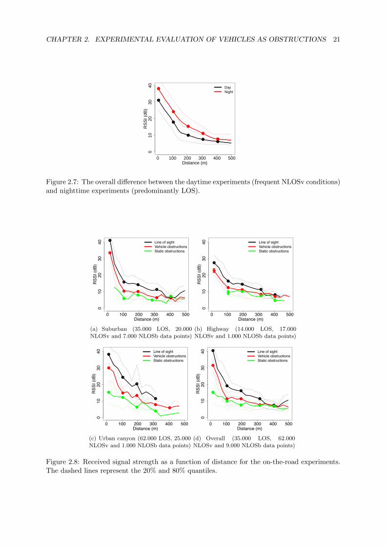
CHAPTER 2. EXPERIMENTAL EVALUATION OF VEHICLES AS OBSTRUCTIONS 21
0 100 200 300 400 500
010
2030
40
●
●
●
●
●
●
●
●
●
●
DayNight
Distance (m)
RS
SI (
dB)
Figure 2.7: The overall difference between the daytime experiments (frequent NLOSv conditions)and nighttime experiments (predominantly LOS).
0 100 200 300 400 500
010
2030
40
●
●
●
●
●
●
● ●
● ●●
●
●
●
Line of sightVehicle obstructionsStatic obstructions
Distance (m)
RSSI
(dB)
(a) Suburban (35.000 LOS, 20.000NLOSv and 7.000 NLOSb data points)
0 100 200 300 400 500
010
2030
40
●
●
●
●
●
●
●
●
●
●
●●
●
●
Line of sightVehicle obstructionsStatic obstructions
Distance (m)
RSSI
(dB)
(b) Highway (14.000 LOS, 17.000NLOSv and 1.000 NLOSb data points)
0 100 200 300 400 500
010
2030
40
●
●
●
●
●
●
●
●
●
●
●
●
●
Line of sightVehicle obstructionsStatic obstructions
Distance (m)
RSSI
(dB)
(c) Urban canyon (62.000 LOS, 25.000NLOSv and 1.000 NLOSb data points)
0 100 200 300 400 500
010
2030
40 ●
●
●
●
●
●
● ●
●●
●
●
● ● ●
Line of sightVehicle obstructionsStatic obstructions
Distance (m)
RSSI
(dB)
(d) Overall (35.000 LOS, 62.000NLOSv and 9.000 NLOSb data points)
Figure 2.8: Received signal strength as a function of distance for the on-the-road experiments.The dashed lines represent the 20% and 80% quantiles.
Chapter 3
Modeling Vehicles as Obstacles in
VANETs
A thorough understanding of the communications channel between vehicles is essential for real-
istic modeling of Vehicular Ad Hoc Networks (VANETs) and the development of related tech-
nology and applications. The impact of vehicles as obstacles on vehicle-to-vehicle (V2V) com-
munication has been largely neglected in VANET research, especially in simulations. Useful
models accounting for vehicles as obstacles must satisfy a number of requirements, most notably
accurate positioning, realistic mobility patterns, realistic propagation characteristics, and man-
ageable complexity. We present a model that satisfies all of these requirements [15]. Vehicles are
modeled as physical obstacles affecting the V2V communication. The proposed model accounts
for vehicles as three-dimensional obstacles and takes into account their impact on the LOS
obstruction, received signal power, and the packet reception rate. We utilize the experiments
reported in Chapter 2 along with two highway datasets containing vehicle locations collected
via stereoscopic aerial photography to test our proposed model. We confirm the importance of
modeling the effects of obstructing vehicles through experimental measurements. By obstruct-
ing the LOS, vehicles induce significant attenuation and packet loss. The algorithm behind the
proposed model allows for computationally efficient implementation in VANET simulators. It
is also shown that by modeling the vehicles as obstacles, significant realism can be added to
existing simulators with relevant implications on the design of upper layer protocols.
22
CHAPTER 3. MODELING VEHICLES AS OBSTACLES IN VANETS 23
3.1 Motivation
Vehicle to vehicle (V2V) communication is proposed as the communication paradigm for a
number of traffic safety ( [4, 40], traffic management ( [41]), and infotainment applications
( [4, 42, 43]). In the previous chapter we have shown that in V2V communication, due to
the relatively low elevation of the antennas on the communicating vehicles, other vehicles act as
obstacles to the signal, often affecting propagation even more than static obstacles (e.g., buildings
or hills), especially in the case of an open road. As noted in a recent survey on Vehicular Ad
Hoc Network (VANET) simulators [26], state of the art VANET simulators such as NS-2 [19],
JiST/SWANS/STRAW [44], and NCTU-NS [45], consider the vehicles as dimensionless entities
that have no influence on signal propagation. One reason lies in the fact that realistic propagation
models for such highly dynamic networks are generally deemed to be computationally expensive
(e.g., ray-tracing [46]), and mobile obstacles increase the complexity even further. Simplified
stochastic radio models, which rely on the statistical properties of the chosen environment and
do not account for the specific obstacles in the region of interest, are thus preferred for use in
simulators, and are believed to offer reasonable approximations at low computational cost [1]. A
recent study showed, however, that stochastic radio models do not provide satisfying accuracy for
typical VANET scenarios [2]. On the other extreme, topography-specific, highly realistic channel
models (such as the one presented in [12]) yield results that are in very good agreement with the
real world, albeit at a price. These models are computationally too expensive and bound to a
specific location (e.g., a particular neighborhood in a city, such as in [12]) to be practically useful
for simulations. For these reasons, such models are not implemented in VANET simulators.
Hence, there exists a need for accurate and efficient V2V channel models. To provide such
a model, we incorporate vehicles as obstacles and present a method to analyze the existence
of the LOS component of the signal for each communicating pair. The focus on the existence
of the LOS component was motivated by the recent experimental V2V studies reported in [47]
and [34]. These studies showed that, when existent, the LOS component of the signal carries
orders of magnitude more energy than the remaining components (e.g., due to reflection or
diffraction). This effect was shown to be particularly pronounced in highway environments. We
therefore analyze the data collected on Portuguese highways to show that, as physical obstacles,
vehicles have a significant impact on signal propagation, by frequently obstructing the LOS

CHAPTER 3. MODELING VEHICLES AS OBSTACLES IN VANETS 24
between the communicating vehicles. Based on the (non-)existence of LOS, we implemented a
simple and efficient model for vehicles as obstacles and showed that for the proposed VANET
communication standard, the Dedicated Short Range Communication (DSRC) [23], the signal
attenuation due to the obstructing vehicles is significant. To further verify the predictions
of the proposed model, we conducted empirical measurements which corroborated the results
regarding the signal attenuation due to vehicles. Not modeling the vehicles as obstacles thus
leads to unrealistic assumptions about the physical layer, and this was shown to have significant
implications on the behavior of the upper layers of the protocol stack (e.g., [1], [14], and [31]).
Our main contributions are as follows.
1. By analyzing the real-world data, we quantify the impact of vehicles as obstacles on V2V
communication in terms of LOS obstruction. The results show that the obstructing vehicles
have a significant impact on LOS in both sparse and dense vehicular networks and should
therefore be included in V2V channel modeling in order to obtain more realistic simulation
results.
2. Based on the LOS obstruction analysis, we develop a model for incorporating the vehicles as
obstacles in VANET simulators. The model encompasses calculation of LOS obstruction,
as well as a simple signal propagation model to characterize the effects of obstructing
vehicles on the received signal power and the packet reception ratio. We confirm the
results of the model by performing empirical V2V measurements.
3. In order to make the proposed model suitable for implementation in VANET simulation
environments, we designed it with the following characteristics in mind:
• suitability for any VANET environment (e.g., urban, suburban, highway) with any
vehicle density;
• topology/location independence;
• feasible implementation in VANET simulators; and
• complementarity and compatibility with VANET signal propagation models for static
obstacles (e.g., buildings, foliage, etc).
The results obtained by employing the proposed model show that significant improvements
can be obtained with regards to the realism of the simulation results, at the same time
CHAPTER 3. MODELING VEHICLES AS OBSTACLES IN VANETS 25
maintaining relatively low computational cost. For this reason, we argue that such model
needs to be implemented in VANET simulators in order to increase the credibility of
simulation results.
The rest of the chapter is organized as follows. Section 3.2 describes previous work on
channel characterization in V2V communication. The methodology for evaluating the impact
of vehicles on LOS and signal behavior is described in Section 3.3, whereas Section 3.4 presents
the requirements of the proposed model and the means to obtain the required data. Section 3.5
highlights the obtained results. Finally, Section 3.6 concludes the chapter.
3.2 Related Work
Our approach towards V2V communication is based on the following hypothesis: the low heights
of the antennas in V2V communication system suggests that other vehicles can act as obsta-
cles for signal propagation, most notably by obstructing the LOS between the communicating
vehicles. Numerous studies, both experimental and analytical (e.g., [13] and [17]), have shown
that LOS and non-LOS (NLOS) scenarios must be separately modeled in VANETs, because the
resulting channel characteristics are fundamentally different.
Several other experimental studies point out that other vehicles apart from the transmitter
and receiver could be an important factor for the signal propagation (mainly by obstructing the
LOS, thus decreasing the received signal power) and therefore should be included in channel
modeling (e.g., [32, 36,38]).
Wang et al. in [6] analyzed the state of the art in V2V channel measurement and modeling.
Based on the approach of modeling the environment (geometrically or non-geometrically), and
the distribution of objects in the environment (stochastic or deterministic), three main types of
models were identified: non-geometrical stochastic models, geometry-based deterministic mod-
els, and geometry-based stochastic models. Using this classification, we present an overview of
the existing research on V2V communication and channel modeling with respect to vehicles as
obstacles.
CHAPTER 3. MODELING VEHICLES AS OBSTACLES IN VANETS 26
3.2.1 Non-Geometrical Stochastic Models
Otto et al. in [14] performed experiments at the 2.4 GHz frequency band in urban, suburban,
and open road environments. Although the study focused on static obstacles such as buildings,
the results showed a significantly worse signal reception on the same open road during the traffic
heavy, rush hour period when compared to a no traffic, late night period. The measurements for
the rush hour period showed a mean path loss exponent of 3.31 and a shadowing deviation of
4.84 dB, whereas in the late night period the mean path loss exponent was 3.1 with a shadowing
deviation of 3.23 dB. The observed difference can only be attributed to other vehicles obstructing
the signal, since all other system parameters remained the same.
Cheng et al. in [24] performed measurements of the V2V channel in the 5.9 GHz frequency
band and pointed out that vehicles as obstacles are the most probable cause for the difference
in received signal power between the obtained experimental measurements and the dual slope
piecewise linear channel model used in that study. Extensive measurement campaigns reported in
[35] analyzed urban, suburban, and highway environments with two levels of traffic density (high
and low). The measurements showed significantly differing channel properties in low and high
traffic scenarios. Based on the measurements, several V2V channel models were proposed. The
presented models are specific for a given environment and vehicle traffic density. A simple error
model for V2V communication was presented in [48], where the authors differentiate the LOS
and NLOS communication due to vehicles using a highly abstracted model where a threshold
distance is used to separate the LOS and NLOS communication. As noted in the same paper,
higher realism requires a more detailed channel model that differentiates between the LOS and
NLOS communication induced by vehicles.
3.2.2 Geometry-Based Deterministic Models
A highly realistic model, based on optical ray-tracing was presented in [12]. The model encom-
passes all objects in the analyzed environment (both static and mobile) and evaluates the signal
behavior by analyzing the 50 strongest propagation paths between the communicating pair. The
model was compared against experimental measurements and showed close agreement. However,
the realism of the model is achieved at the cost of high computational complexity and location-
specific modeling. Even with the recent advances in optimizing the execution of ray-tracing
CHAPTER 3. MODELING VEHICLES AS OBSTACLES IN VANETS 27
models [49], the method remains computationally too expensive to be implemented in VANET
simulators. Additionally, detailed knowledge about the topology of the analyzed environment is
necessary in order to accurately model the channel.
3.2.3 Geometry-Based Stochastic Models
Karedal et al. in [50] designed a model for the V2V channel based on extensive measurements
performed in highway and suburban environment at the 5.2 GHz frequency band. The model
distributes the vehicles as well as other objects at random locations and analyzes four distinct
signal components: LOS, discrete components from mobile objects, discrete components from
static objects, and diffuse scattering. Based on the obtained measurement data, a set of model
parameters for the two environments is prescribed, and the non-stationarity of the V2V channel
can be captured by employing a mobility model for the vehicles (it was shown in [51] that the
wide-sense stationary uncorrelated scattering assumption does not hold for the V2V channel).
Cheng et al. in [52] presented a MIMO channel model that takes into account the LOS, single-
bounced rays, and double-bounced rays by employing a combined two-ring and ellipse model.
By properly defining the parameters, the model can be used in various V2V environments with
varying vehicle densities. Due to the static nature of the employed geometric model, the non-
stationarity of the V2V channel can not be captured.
With regards to the implementation of vehicles as obstacles in simulators, virtually all of
the state of the art VANET simulators neglect the impact of vehicles as obstacles on signal
propagation, mainly due to the lack of an appropriate methodology capable of incorporating the
effect of vehicles both realistically and efficiently.
To the best of our knowledge, up to now there has been no study that focused on vehicles as
obstacles by systematically quantifying their impact on LOS and consequently on the received
signal power. Apart from quantifying the impact of vehicles, we present a computationally
efficient model for the implementation of vehicles as obstacles in VANET simulators. Our
model can be seen as a simplified geometry-based deterministic model.
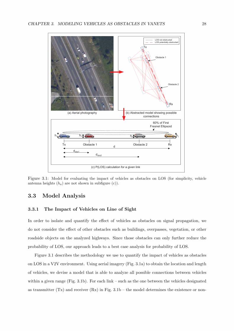
CHAPTER 3. MODELING VEHICLES AS OBSTACLES IN VANETS 28
Tx
Rx
Obstacle 1
Obstacle 2
(a) Aerial photography (b) Abstracted model showing possible
connections
LOS not obstructed
LOS potentially obstructed
60% of First
Fresnel Ellipsoid
Tx RxObstacle 1 Obstacle 2d
dobs1
dobs2
h1h i h jh2
(c) P(LOS) calculation for a given link
Figure 3.1: Model for evaluating the impact of vehicles as obstacles on LOS (for simplicity, vehicleantenna heights (ha) are not shown in subfigure (c)).
3.3 Model Analysis
3.3.1 The Impact of Vehicles on Line of Sight
In order to isolate and quantify the effect of vehicles as obstacles on signal propagation, we
do not consider the effect of other obstacles such as buildings, overpasses, vegetation, or other
roadside objects on the analyzed highways. Since those obstacles can only further reduce the
probability of LOS, our approach leads to a best case analysis for probability of LOS.
Figure 3.1 describes the methodology we use to quantify the impact of vehicles as obstacles
on LOS in a V2V environment. Using aerial imagery (Fig. 3.1a) to obtain the location and length
of vehicles, we devise a model that is able to analyze all possible connections between vehicles
within a given range (Fig. 3.1b). For each link – such as the one between the vehicles designated
as transmitter (Tx) and receiver (Rx) in Fig. 3.1b – the model determines the existence or non-
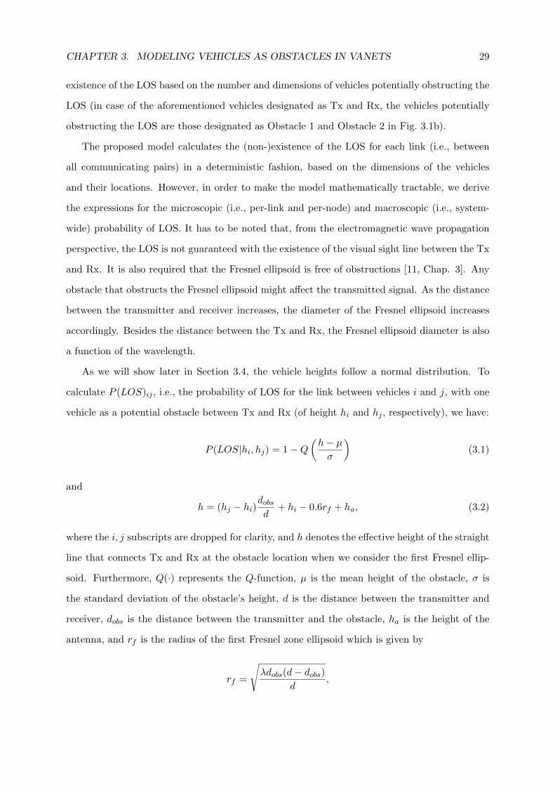
CHAPTER 3. MODELING VEHICLES AS OBSTACLES IN VANETS 29
existence of the LOS based on the number and dimensions of vehicles potentially obstructing the
LOS (in case of the aforementioned vehicles designated as Tx and Rx, the vehicles potentially
obstructing the LOS are those designated as Obstacle 1 and Obstacle 2 in Fig. 3.1b).
The proposed model calculates the (non-)existence of the LOS for each link (i.e., between
all communicating pairs) in a deterministic fashion, based on the dimensions of the vehicles
and their locations. However, in order to make the model mathematically tractable, we derive
the expressions for the microscopic (i.e., per-link and per-node) and macroscopic (i.e., system-
wide) probability of LOS. It has to be noted that, from the electromagnetic wave propagation
perspective, the LOS is not guaranteed with the existence of the visual sight line between the Tx
and Rx. It is also required that the Fresnel ellipsoid is free of obstructions [11, Chap. 3]. Any
obstacle that obstructs the Fresnel ellipsoid might affect the transmitted signal. As the distance
between the transmitter and receiver increases, the diameter of the Fresnel ellipsoid increases
accordingly. Besides the distance between the Tx and Rx, the Fresnel ellipsoid diameter is also
a function of the wavelength.
As we will show later in Section 3.4, the vehicle heights follow a normal distribution. To
calculate P (LOS)ij , i.e., the probability of LOS for the link between vehicles i and j, with one
vehicle as a potential obstacle between Tx and Rx (of height hi and hj , respectively), we have:
P (LOS|hi, hj) = 1−Q(h− µσ
)(3.1)
and
h = (hj − hi)dobsd
+ hi − 0.6rf + ha, (3.2)
where the i, j subscripts are dropped for clarity, and h denotes the effective height of the straight
line that connects Tx and Rx at the obstacle location when we consider the first Fresnel ellip-
soid. Furthermore, Q(·) represents the Q-function, µ is the mean height of the obstacle, σ is
the standard deviation of the obstacle’s height, d is the distance between the transmitter and
receiver, dobs is the distance between the transmitter and the obstacle, ha is the height of the
antenna, and rf is the radius of the first Fresnel zone ellipsoid which is given by
rf =
√λdobs(d− dobs)
d,

CHAPTER 3. MODELING VEHICLES AS OBSTACLES IN VANETS 30
with λ denoting the wavelength. We use the appropriate λ for the proposed standard for VANET
communication (DSRC), which operates in the 5.9 GHz frequency band. In our studies, we
assume that the antennas are located on top of the vehicles in the middle of the roof (which
was experimentally shown to be the overall optimum placement of the antenna [31]), and we
set the ha to 10 cm. As a general rule commonly used in literature, LOS is considered to be
unobstructed if intermediate vehicles obstruct the first Fresnel ellipsoid by less than 40% [11,
Chap. 3]. Furthermore, for No vehicles as potential obstacles between the Tx and Rx, we get
(see Fig. 3.1c)
P (LOS|hi, hj) =No∏k=1
[1−Q
(hk − µkσk
)], (3.3)
where hk is the effective height of the straight line that connects Tx and Rx at the location
of the k-th obstacle considering the first Fresnel ellipsoid, µk is the mean height of the k-th
obstacle, and σk is the standard deviation of the height of the k-th obstacle.
Averaging over the transmitter and receiver antenna heights with respect to the road, we
obtain the unconditional P (LOS)ij
P (LOS)ij =
∫ ∫P (LOS|hi, hj)p(hi)p(hj)dhidhj , (3.4)
where p(hi) and p(hj) are the probability density functions for the transmitter and receiver
antenna heights with respect to the road, respectively.
The average probability of LOS for a given vehicle i, P (LOS)i, and all its Ni neighbors is
defined as
P (LOS)i =1
Ni
Ni∑j=1
P (LOS)ij (3.5)
To determine the system-wide ratio of LOS paths blocked by other vehicles, we average P (LOS)i
over all Nv vehicles in the system, yielding
P (LOS) =1
Nv
Nv∑i=1
P (LOS)i. (3.6)
Furthermore, we analyze the behavior of the probability of LOS for a given vehicle i over
time. Let us denote the i-th vehicle probability of LOS at a given time t as P (LOS)ti. We define
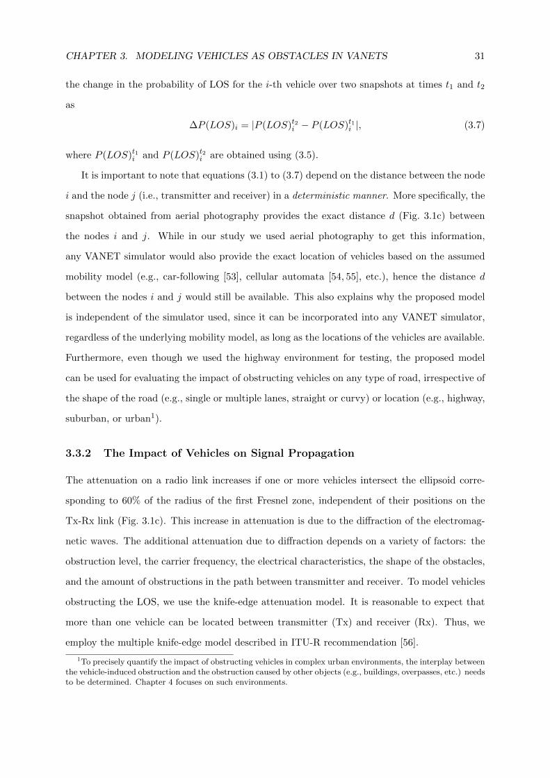
CHAPTER 3. MODELING VEHICLES AS OBSTACLES IN VANETS 31
the change in the probability of LOS for the i-th vehicle over two snapshots at times t1 and t2
as
∆P (LOS)i = |P (LOS)t2i − P (LOS)t1i |, (3.7)
where P (LOS)t1i and P (LOS)t2i are obtained using (3.5).
It is important to note that equations (3.1) to (3.7) depend on the distance between the node
i and the node j (i.e., transmitter and receiver) in a deterministic manner. More specifically, the
snapshot obtained from aerial photography provides the exact distance d (Fig. 3.1c) between
the nodes i and j. While in our study we used aerial photography to get this information,
any VANET simulator would also provide the exact location of vehicles based on the assumed
mobility model (e.g., car-following [53], cellular automata [54, 55], etc.), hence the distance d
between the nodes i and j would still be available. This also explains why the proposed model
is independent of the simulator used, since it can be incorporated into any VANET simulator,
regardless of the underlying mobility model, as long as the locations of the vehicles are available.
Furthermore, even though we used the highway environment for testing, the proposed model
can be used for evaluating the impact of obstructing vehicles on any type of road, irrespective of
the shape of the road (e.g., single or multiple lanes, straight or curvy) or location (e.g., highway,
suburban, or urban1).
3.3.2 The Impact of Vehicles on Signal Propagation
The attenuation on a radio link increases if one or more vehicles intersect the ellipsoid corre-
sponding to 60% of the radius of the first Fresnel zone, independent of their positions on the
Tx-Rx link (Fig. 3.1c). This increase in attenuation is due to the diffraction of the electromag-
netic waves. The additional attenuation due to diffraction depends on a variety of factors: the
obstruction level, the carrier frequency, the electrical characteristics, the shape of the obstacles,
and the amount of obstructions in the path between transmitter and receiver. To model vehicles
obstructing the LOS, we use the knife-edge attenuation model. It is reasonable to expect that
more than one vehicle can be located between transmitter (Tx) and receiver (Rx). Thus, we
employ the multiple knife-edge model described in ITU-R recommendation [56].
1To precisely quantify the impact of obstructing vehicles in complex urban environments, the interplay betweenthe vehicle-induced obstruction and the obstruction caused by other objects (e.g., buildings, overpasses, etc.) needsto be determined. Chapter 4 focuses on such environments.
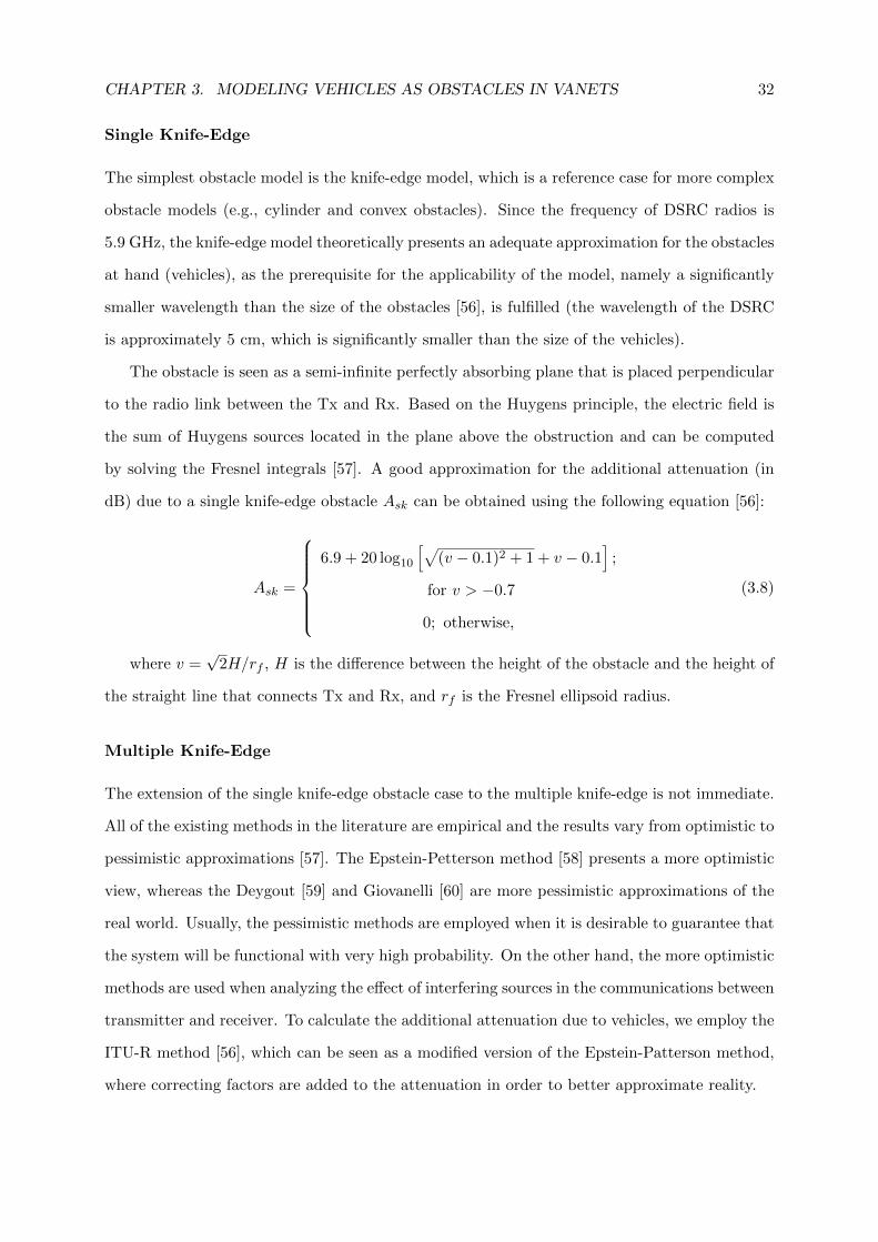
CHAPTER 3. MODELING VEHICLES AS OBSTACLES IN VANETS 32
Single Knife-Edge
The simplest obstacle model is the knife-edge model, which is a reference case for more complex
obstacle models (e.g., cylinder and convex obstacles). Since the frequency of DSRC radios is
5.9 GHz, the knife-edge model theoretically presents an adequate approximation for the obstacles
at hand (vehicles), as the prerequisite for the applicability of the model, namely a significantly
smaller wavelength than the size of the obstacles [56], is fulfilled (the wavelength of the DSRC
is approximately 5 cm, which is significantly smaller than the size of the vehicles).
The obstacle is seen as a semi-infinite perfectly absorbing plane that is placed perpendicular
to the radio link between the Tx and Rx. Based on the Huygens principle, the electric field is
the sum of Huygens sources located in the plane above the obstruction and can be computed
by solving the Fresnel integrals [57]. A good approximation for the additional attenuation (in
dB) due to a single knife-edge obstacle Ask can be obtained using the following equation [56]:
Ask =
6.9 + 20 log10
[√(v − 0.1)2 + 1 + v − 0.1
];
for v > −0.7
0; otherwise,
(3.8)
where v =√
2H/rf , H is the difference between the height of the obstacle and the height of
the straight line that connects Tx and Rx, and rf is the Fresnel ellipsoid radius.
Multiple Knife-Edge
The extension of the single knife-edge obstacle case to the multiple knife-edge is not immediate.
All of the existing methods in the literature are empirical and the results vary from optimistic to
pessimistic approximations [57]. The Epstein-Petterson method [58] presents a more optimistic
view, whereas the Deygout [59] and Giovanelli [60] are more pessimistic approximations of the
real world. Usually, the pessimistic methods are employed when it is desirable to guarantee that
the system will be functional with very high probability. On the other hand, the more optimistic
methods are used when analyzing the effect of interfering sources in the communications between
transmitter and receiver. To calculate the additional attenuation due to vehicles, we employ the
ITU-R method [56], which can be seen as a modified version of the Epstein-Patterson method,
where correcting factors are added to the attenuation in order to better approximate reality.
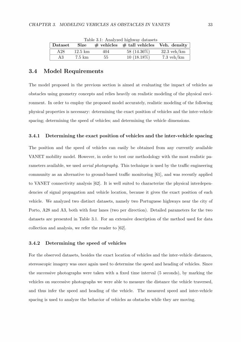
CHAPTER 3. MODELING VEHICLES AS OBSTACLES IN VANETS 33
Table 3.1: Analyzed highway datasetsDataset Size # vehicles # tall vehicles Veh. density
A28 12.5 km 404 58 (14.36%) 32.3 veh/km
A3 7.5 km 55 10 (18.18%) 7.3 veh/km
3.4 Model Requirements
The model proposed in the previous section is aimed at evaluating the impact of vehicles as
obstacles using geometry concepts and relies heavily on realistic modeling of the physical envi-
ronment. In order to employ the proposed model accurately, realistic modeling of the following
physical properties is necessary: determining the exact position of vehicles and the inter-vehicle
spacing; determining the speed of vehicles; and determining the vehicle dimensions.
3.4.1 Determining the exact position of vehicles and the inter-vehicle spacing
The position and the speed of vehicles can easily be obtained from any currently available
VANET mobility model. However, in order to test our methodology with the most realistic pa-
rameters available, we used aerial photography. This technique is used by the traffic engineering
community as an alternative to ground-based traffic monitoring [61], and was recently applied
to VANET connectivity analysis [62]. It is well suited to characterize the physical interdepen-
dencies of signal propagation and vehicle location, because it gives the exact position of each
vehicle. We analyzed two distinct datasets, namely two Portuguese highways near the city of
Porto, A28 and A3, both with four lanes (two per direction). Detailed parameters for the two
datasets are presented in Table 3.1. For an extensive description of the method used for data
collection and analysis, we refer the reader to [62].
3.4.2 Determining the speed of vehicles
For the observed datasets, besides the exact location of vehicles and the inter-vehicle distances,
stereoscopic imagery was once again used to determine the speed and heading of vehicles. Since
the successive photographs were taken with a fixed time interval (5 seconds), by marking the
vehicles on successive photographs we were able to measure the distance the vehicle traversed,
and thus infer the speed and heading of the vehicle. The measured speed and inter-vehicle
spacing is used to analyze the behavior of vehicles as obstacles while they are moving.
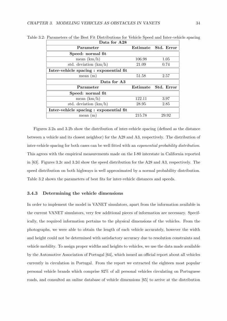
CHAPTER 3. MODELING VEHICLES AS OBSTACLES IN VANETS 34
Table 3.2: Parameters of the Best Fit Distributions for Vehicle Speed and Inter-vehicle spacingData for A28
Parameter Estimate Std. Error
Speed: normal fit
mean (km/h) 106.98 1.05
std. deviation (km/h) 21.09 0.74
Inter-vehicle spacing : exponential fit
mean (m) 51.58 2.57
Data for A3
Parameter Estimate Std. Error
Speed: normal fit
mean (km/h) 122.11 3.97
std. deviation (km/h) 28.95 2.85
Inter-vehicle spacing : exponential fit
mean (m) 215.78 29.92
Figures 3.2a and 3.2b show the distribution of inter-vehicle spacing (defined as the distance
between a vehicle and its closest neighbor) for the A28 and A3, respectively. The distribution of
inter-vehicle spacing for both cases can be well fitted with an exponential probability distribution.
This agrees with the empirical measurements made on the I-80 interstate in California reported
in [63]. Figures 3.2c and 3.2d show the speed distribution for the A28 and A3, respectively. The
speed distribution on both highways is well approximated by a normal probability distribution.
Table 3.2 shows the parameters of best fits for inter-vehicle distances and speeds.
3.4.3 Determining the vehicle dimensions
In order to implement the model in VANET simulators, apart from the information available in
the current VANET simulators, very few additional pieces of information are necessary. Specif-
ically, the required information pertains to the physical dimensions of the vehicles. From the
photographs, we were able to obtain the length of each vehicle accurately, however the width
and height could not be determined with satisfactory accuracy due to resolution constraints and
vehicle mobility. To assign proper widths and heights to vehicles, we use the data made available
by the Automotive Association of Portugal [64], which issued an official report about all vehicles
currently in circulation in Portugal. From the report we extracted the eighteen most popular
personal vehicle brands which comprise 92% of all personal vehicles circulating on Portuguese
roads, and consulted an online database of vehicle dimensions [65] to arrive at the distribution
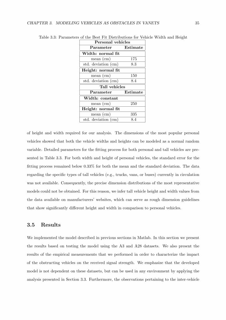
CHAPTER 3. MODELING VEHICLES AS OBSTACLES IN VANETS 35
Table 3.3: Parameters of the Best Fit Distributions for Vehicle Width and HeightPersonal vehicles
Parameter Estimate
Width: normal fit
mean (cm) 175
std. deviation (cm) 8.3
Height: normal fit
mean (cm) 150
std. deviation (cm) 8.4
Tall vehicles
Parameter Estimate
Width: constant
mean (cm) 250
Height: normal fit
mean (cm) 335
std. deviation (cm) 8.4
of height and width required for our analysis. The dimensions of the most popular personal
vehicles showed that both the vehicle widths and heights can be modeled as a normal random
variable. Detailed parameters for the fitting process for both personal and tall vehicles are pre-
sented in Table 3.3. For both width and height of personal vehicles, the standard error for the
fitting process remained below 0.33% for both the mean and the standard deviation. The data
regarding the specific types of tall vehicles (e.g., trucks, vans, or buses) currently in circulation
was not available. Consequently, the precise dimension distributions of the most representative
models could not be obtained. For this reason, we infer tall vehicle height and width values from
the data available on manufacturers’ websites, which can serve as rough dimension guidelines
that show significantly different height and width in comparison to personal vehicles.
3.5 Results
We implemented the model described in previous sections in Matlab. In this section we present
the results based on testing the model using the A3 and A28 datasets. We also present the
results of the empirical measurements that we performed in order to characterize the impact
of the obstructing vehicles on the received signal strength. We emphasize that the developed
model is not dependent on these datasets, but can be used in any environment by applying the
analysis presented in Section 3.3. Furthermore, the observations pertaining to the inter-vehicle
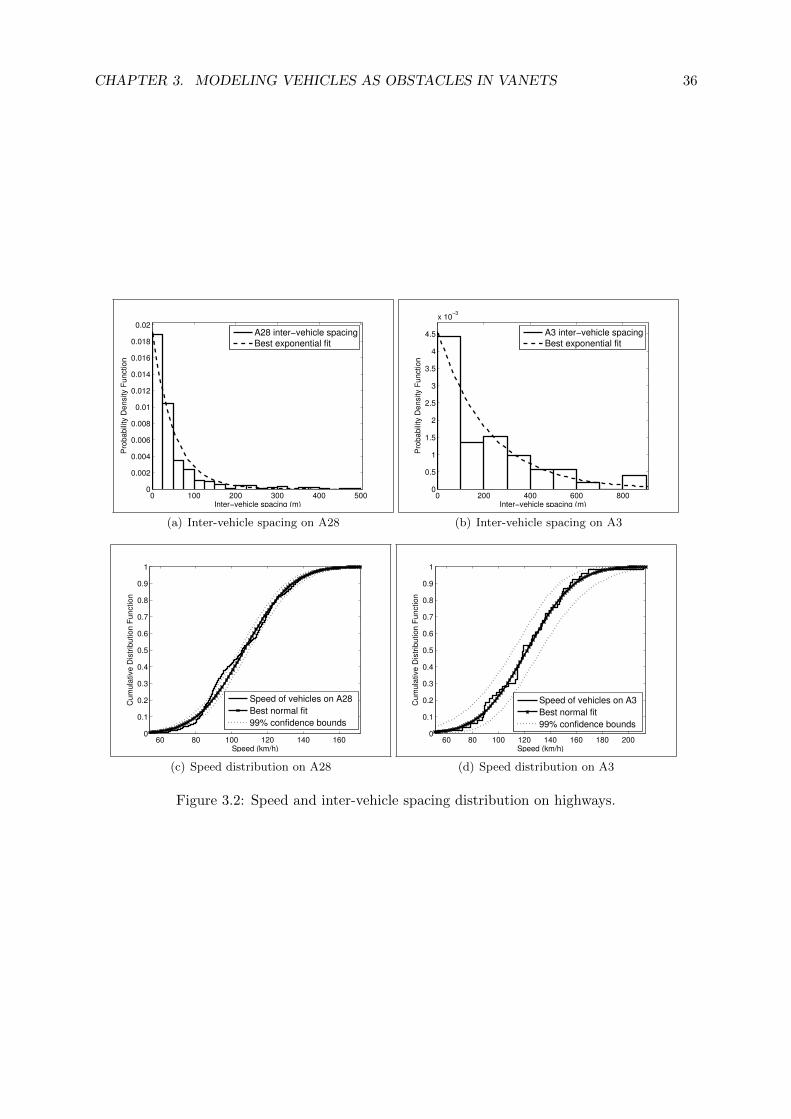
CHAPTER 3. MODELING VEHICLES AS OBSTACLES IN VANETS 36
0 100 200 300 400 5000
0.002
0.004
0.006
0.008
0.01
0.012
0.014
0.016
0.018
0.02
Inter−vehicle spacing (m)
Pro
ba
bili
ty D
en
sity F
un
ctio
n
A28 inter−vehicle spacing
Best exponential fit
(a) Inter-vehicle spacing on A28
0 200 400 600 8000
0.5
1
1.5
2
2.5
3
3.5
4
4.5
x 10−3
Inter−vehicle spacing (m)
Pro
ba
bili
ty D
en
sity F
un
ctio
n
A3 inter−vehicle spacing
Best exponential fit
(b) Inter-vehicle spacing on A3
60 80 100 120 140 1600
0.1
0.2
0.3
0.4
0.5
0.6
0.7
0.8
0.9
1
Speed (km/h)
Cu
mu
lative
Dis
trib
utio
n F
un
ctio
n
Speed of vehicles on A28
Best normal fit
99% confidence bounds
(c) Speed distribution on A28
60 80 100 120 140 160 180 2000
0.1
0.2
0.3
0.4
0.5
0.6
0.7
0.8
0.9
1
Speed (km/h)
Cu
mu
lative
Dis
trib
utio
n F
un
ctio
n
Speed of vehicles on A3
Best normal fit
99% confidence bounds
(d) Speed distribution on A3
Figure 3.2: Speed and inter-vehicle spacing distribution on highways.
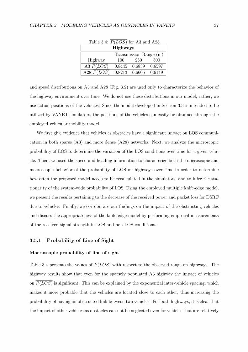
CHAPTER 3. MODELING VEHICLES AS OBSTACLES IN VANETS 37
Table 3.4: P (LOS) for A3 and A28Highways
Transmission Range (m)Highway 100 250 500
A3 P (LOS) 0.8445 0.6839 0.6597
A28 P (LOS) 0.8213 0.6605 0.6149
and speed distributions on A3 and A28 (Fig. 3.2) are used only to characterize the behavior of
the highway environment over time. We do not use these distributions in our model; rather, we
use actual positions of the vehicles. Since the model developed in Section 3.3 is intended to be
utilized by VANET simulators, the positions of the vehicles can easily be obtained through the
employed vehicular mobility model.
We first give evidence that vehicles as obstacles have a significant impact on LOS communi-
cation in both sparse (A3) and more dense (A28) networks. Next, we analyze the microscopic
probability of LOS to determine the variation of the LOS conditions over time for a given vehi-
cle. Then, we used the speed and heading information to characterize both the microscopic and
macroscopic behavior of the probability of LOS on highways over time in order to determine
how often the proposed model needs to be recalculated in the simulators, and to infer the sta-
tionarity of the system-wide probability of LOS. Using the employed multiple knife-edge model,
we present the results pertaining to the decrease of the received power and packet loss for DSRC
due to vehicles. Finally, we corroborate our findings on the impact of the obstructing vehicles
and discuss the appropriateness of the knife-edge model by performing empirical measurements
of the received signal strength in LOS and non-LOS conditions.
3.5.1 Probability of Line of Sight
Macroscopic probability of line of sight
Table 3.4 presents the values of P (LOS) with respect to the observed range on highways. The
highway results show that even for the sparsely populated A3 highway the impact of vehicles
on P (LOS) is significant. This can be explained by the exponential inter-vehicle spacing, which
makes it more probable that the vehicles are located close to each other, thus increasing the
probability of having an obstructed link between two vehicles. For both highways, it is clear that
the impact of other vehicles as obstacles can not be neglected even for vehicles that are relatively
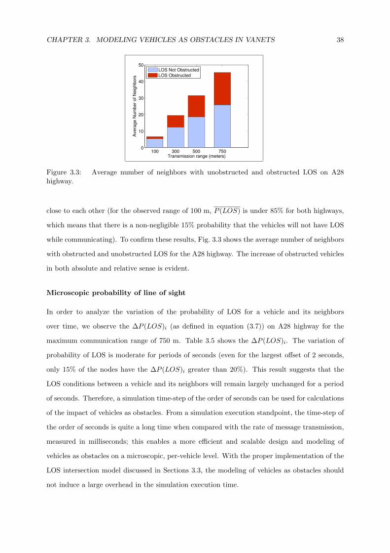
CHAPTER 3. MODELING VEHICLES AS OBSTACLES IN VANETS 38
100 300 500 7500
10
20
30
40
50
Transmission range (meters)
Ave
rag
e N
um
be
r o
f N
eig
hb
ors
LOS Not Obstructed
LOS Obstructed
Figure 3.3: Average number of neighbors with unobstructed and obstructed LOS on A28highway.
close to each other (for the observed range of 100 m, P (LOS) is under 85% for both highways,
which means that there is a non-negligible 15% probability that the vehicles will not have LOS
while communicating). To confirm these results, Fig. 3.3 shows the average number of neighbors
with obstructed and unobstructed LOS for the A28 highway. The increase of obstructed vehicles
in both absolute and relative sense is evident.
Microscopic probability of line of sight
In order to analyze the variation of the probability of LOS for a vehicle and its neighbors
over time, we observe the ∆P (LOS)i (as defined in equation (3.7)) on A28 highway for the
maximum communication range of 750 m. Table 3.5 shows the ∆P (LOS)i. The variation of
probability of LOS is moderate for periods of seconds (even for the largest offset of 2 seconds,
only 15% of the nodes have the ∆P (LOS)i greater than 20%). This result suggests that the
LOS conditions between a vehicle and its neighbors will remain largely unchanged for a period
of seconds. Therefore, a simulation time-step of the order of seconds can be used for calculations
of the impact of vehicles as obstacles. From a simulation execution standpoint, the time-step of
the order of seconds is quite a long time when compared with the rate of message transmission,
measured in milliseconds; this enables a more efficient and scalable design and modeling of
vehicles as obstacles on a microscopic, per-vehicle level. With the proper implementation of the
LOS intersection model discussed in Sections 3.3, the modeling of vehicles as obstacles should
not induce a large overhead in the simulation execution time.

CHAPTER 3. MODELING VEHICLES AS OBSTACLES IN VANETS 39
Table 3.5: Variation of P (LOS)i over time for the observed range of 750 m on A28.∆P (LOS)i in %
Time offset < 5% 5-10% 10-20% >20%
1ms 100% 0% 0% 0%
10ms 99% 1% 0% 0%
100ms 82% 15% 3% 0%
1s 35% 33% 22% 10%
2s 31% 25% 29% 15%
Stochastic properties of line of sight in mobile vehicular network
Figs. 3.2a and 3.2b show that a Poisson process with parameter α can be used to describe the
distribution of vehicles on highways at a given time t. It is reasonable to assume that, for
a vehicular traffic in the free-flow phase, the rate of change of the parameter α over time is
quite slow, thus the Poisson process can be considered homogeneous for a certain amount of
time. This allows us to utilize one of the key properties of homogeneous Poisson processes,
namely stationary increments, which says that if two road segments are of the same length,
the probability distribution function of the number of vehicles over those segments is equal [66].
Therefore, we can conclude that for a certain period of time, the probability distribution function
of the number of vehicles on two road segments will only depend on the size of the segments.
Based on the homogeneity assumption, applying this property on the same segment of the road
but at different times results in identical probability distribution for the number of vehicles.
Therefore, it is expected that the P (LOS) over the observed road segment will not change over
time, as long as the arrival rate α remains constant.
In order to confirm these results, we performed tests using two snapshots of A28 highway
taken on the same road interval 5 seconds one after another. By inferring the speed and heading
of the vehicles from the snapshots, it was possible to accurately interpolate the positions of the
vehicles for 1 ms, 10 ms, 100 ms, 1 s, and 2 s offsets from the first snapshot.
The obtained results showed that the average inter-vehicle spacing remains invariant for the
observed time offsets, thus confirming the first-order stationarity of the underlying Poisson pro-
cess. Similarly, Fig. 3.4 shows that for various communication radii (100 - 750 m), the P (LOS)
does not change for the observed time offsets. Therefore, we can conclude that P (LOS) remains
constant on the observed road interval as long as the arrival rate of the generating Poisson
process remains constant. Thus, the presented P (LOS) results hold for both the instantaneous
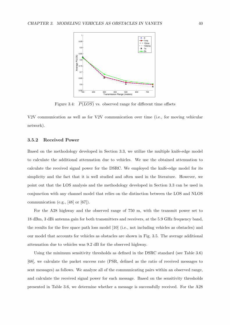
CHAPTER 3. MODELING VEHICLES AS OBSTACLES IN VANETS 40
100 200 300 400 500 600 7000.55
0.6
0.65
0.7
0.75
0.8
0.85
0.9
0.95
1
Transmission Range (meters)
Ave
rag
e P
(LO
S)
0
1ms
10ms100ms
1s
2s
Figure 3.4: P (LOS) vs. observed range for different time offsets
V2V communication as well as for V2V communication over time (i.e., for moving vehicular
network).
3.5.2 Received Power
Based on the methodology developed in Section 3.3, we utilize the multiple knife-edge model
to calculate the additional attenuation due to vehicles. We use the obtained attenuation to
calculate the received signal power for the DSRC. We employed the knife-edge model for its
simplicity and the fact that it is well studied and often used in the literature. However, we
point out that the LOS analysis and the methodology developed in Section 3.3 can be used in
conjunction with any channel model that relies on the distinction between the LOS and NLOS
communication (e.g., [48] or [67]).
For the A28 highway and the observed range of 750 m, with the transmit power set to
18 dBm, 3 dBi antenna gain for both transmitters and receivers, at the 5.9 GHz frequency band,
the results for the free space path loss model [10] (i.e., not including vehicles as obstacles) and
our model that accounts for vehicles as obstacles are shown in Fig. 3.5. The average additional
attenuation due to vehicles was 9.2 dB for the observed highway.
Using the minimum sensitivity thresholds as defined in the DSRC standard (see Table 3.6)
[68], we calculate the packet success rate (PSR, defined as the ratio of received messages to
sent messages) as follows. We analyze all of the communicating pairs within an observed range,
and calculate the received signal power for each message. Based on the sensitivity thresholds
presented in Table 3.6, we determine whether a message is successfully received. For the A28
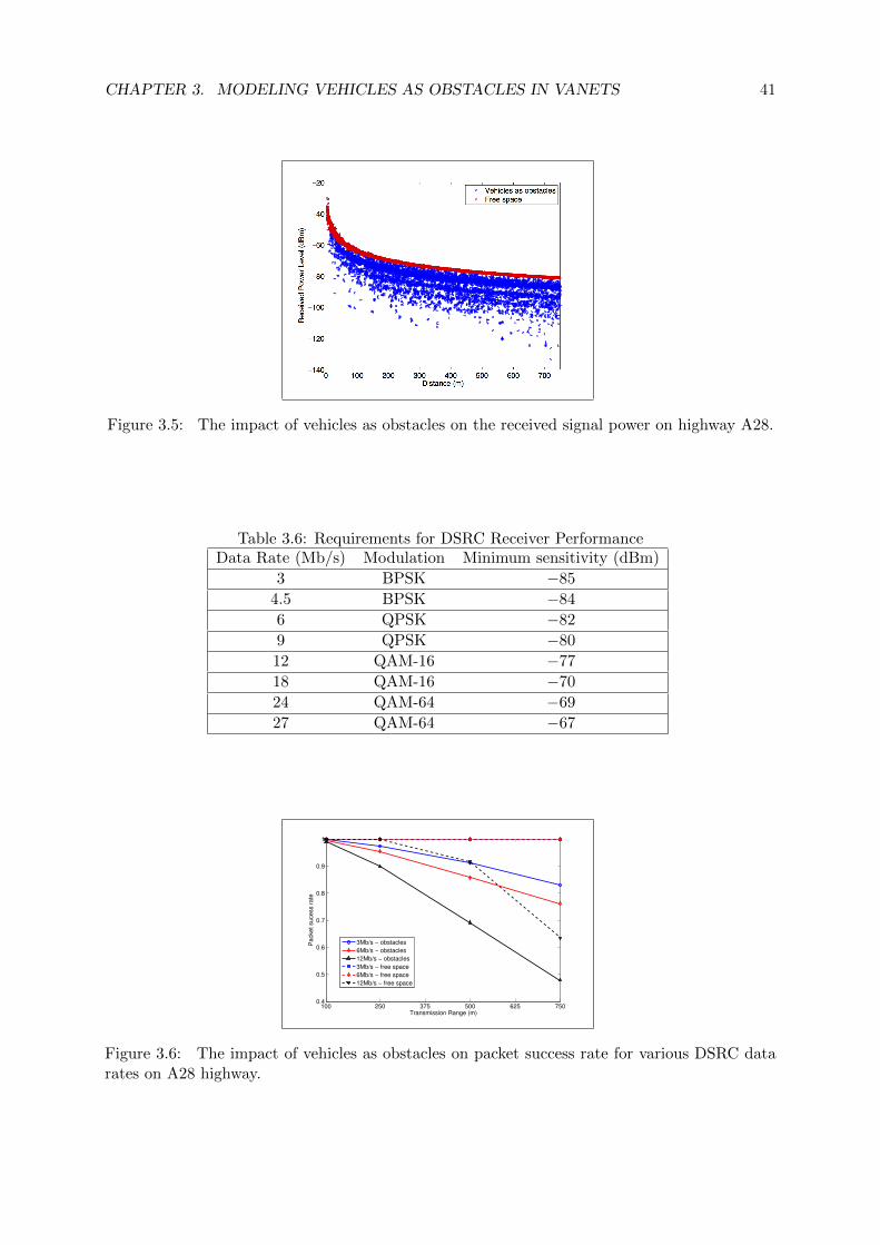
CHAPTER 3. MODELING VEHICLES AS OBSTACLES IN VANETS 41
Figure 3.5: The impact of vehicles as obstacles on the received signal power on highway A28.
Table 3.6: Requirements for DSRC Receiver PerformanceData Rate (Mb/s) Modulation Minimum sensitivity (dBm)
3 BPSK −85
4.5 BPSK −84
6 QPSK −82
9 QPSK −80
12 QAM-16 −77
18 QAM-16 −70
24 QAM-64 −69
27 QAM-64 −67
100 250 375 500 625 7500.4
0.5
0.6
0.7
0.8
0.9
1
Transmission Range (m)
Pa
cke
t su
ce
ss r
ate
3Mb/s − obstacles
6Mb/s − obstacles
12Mb/s − obstacles
3Mb/s − free space
6Mb/s − free space
12Mb/s − free space
Figure 3.6: The impact of vehicles as obstacles on packet success rate for various DSRC datarates on A28 highway.
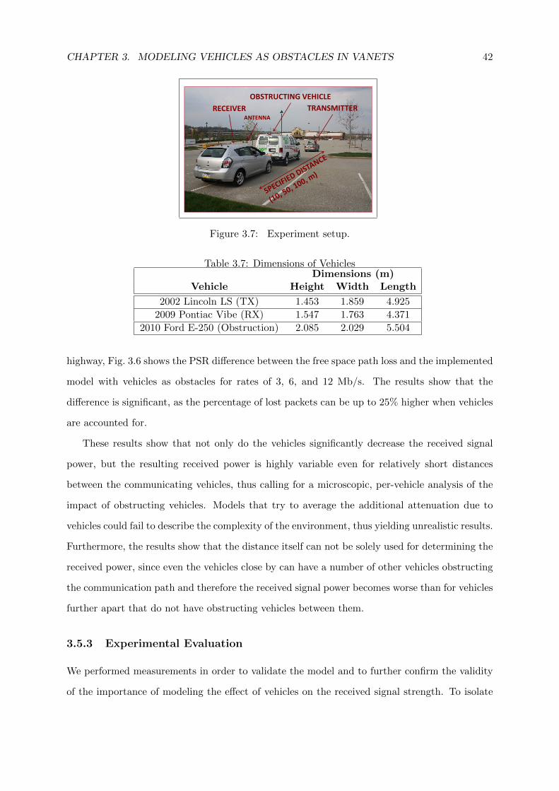
CHAPTER 3. MODELING VEHICLES AS OBSTACLES IN VANETS 42
OBSTRUCTING VEHICLE
TRANSMITTERRECEIVER TRANSMITTERRECEIVER
ANTENNA
Figure 2. Static experiment.
Figure 3.7: Experiment setup.
Table 3.7: Dimensions of VehiclesDimensions (m)
Vehicle Height Width Length
2002 Lincoln LS (TX) 1.453 1.859 4.925
2009 Pontiac Vibe (RX) 1.547 1.763 4.371
2010 Ford E-250 (Obstruction) 2.085 2.029 5.504
highway, Fig. 3.6 shows the PSR difference between the free space path loss and the implemented
model with vehicles as obstacles for rates of 3, 6, and 12 Mb/s. The results show that the
difference is significant, as the percentage of lost packets can be up to 25% higher when vehicles
are accounted for.
These results show that not only do the vehicles significantly decrease the received signal
power, but the resulting received power is highly variable even for relatively short distances
between the communicating vehicles, thus calling for a microscopic, per-vehicle analysis of the
impact of obstructing vehicles. Models that try to average the additional attenuation due to
vehicles could fail to describe the complexity of the environment, thus yielding unrealistic results.
Furthermore, the results show that the distance itself can not be solely used for determining the
received power, since even the vehicles close by can have a number of other vehicles obstructing
the communication path and therefore the received signal power becomes worse than for vehicles
further apart that do not have obstructing vehicles between them.
3.5.3 Experimental Evaluation
We performed measurements in order to validate the model and to further confirm the validity
of the importance of modeling the effect of vehicles on the received signal strength. To isolate
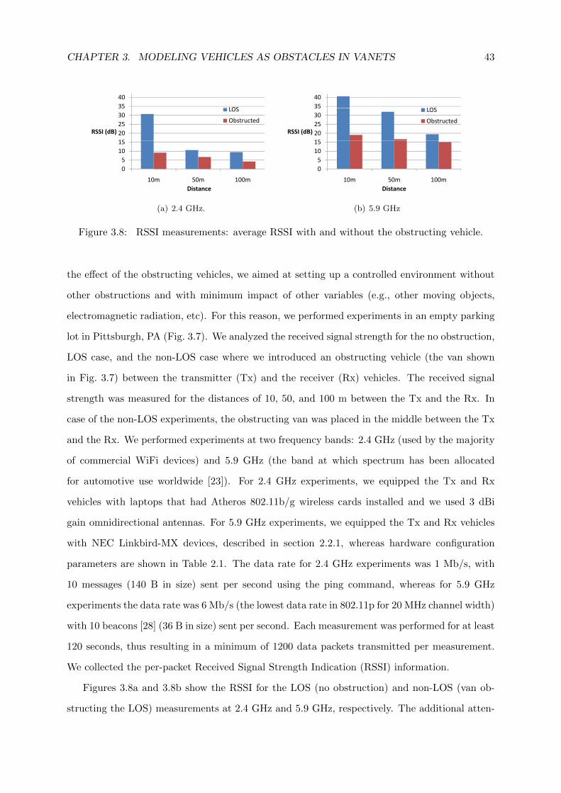
CHAPTER 3. MODELING VEHICLES AS OBSTACLES IN VANETS 43
35
40
LOS
15
20
25
30
35
RSSI (dB)
LOS
Obstructed
0
5
10
15
10m 50m 100m
Distance
(a) 2.4 GHz.
35
40
LOS
15
20
25
30
35
RSSI (dB)
LOS
Obstructed
0
5
10
15
10m 50m 100m
Distance
(b) 5.9 GHz
Figure 3.8: RSSI measurements: average RSSI with and without the obstructing vehicle.
the effect of the obstructing vehicles, we aimed at setting up a controlled environment without
other obstructions and with minimum impact of other variables (e.g., other moving objects,
electromagnetic radiation, etc). For this reason, we performed experiments in an empty parking
lot in Pittsburgh, PA (Fig. 3.7). We analyzed the received signal strength for the no obstruction,
LOS case, and the non-LOS case where we introduced an obstructing vehicle (the van shown
in Fig. 3.7) between the transmitter (Tx) and the receiver (Rx) vehicles. The received signal
strength was measured for the distances of 10, 50, and 100 m between the Tx and the Rx. In
case of the non-LOS experiments, the obstructing van was placed in the middle between the Tx
and the Rx. We performed experiments at two frequency bands: 2.4 GHz (used by the majority
of commercial WiFi devices) and 5.9 GHz (the band at which spectrum has been allocated
for automotive use worldwide [23]). For 2.4 GHz experiments, we equipped the Tx and Rx
vehicles with laptops that had Atheros 802.11b/g wireless cards installed and we used 3 dBi
gain omnidirectional antennas. For 5.9 GHz experiments, we equipped the Tx and Rx vehicles
with NEC Linkbird-MX devices, described in section 2.2.1, whereas hardware configuration
parameters are shown in Table 2.1. The data rate for 2.4 GHz experiments was 1 Mb/s, with
10 messages (140 B in size) sent per second using the ping command, whereas for 5.9 GHz
experiments the data rate was 6 Mb/s (the lowest data rate in 802.11p for 20 MHz channel width)
with 10 beacons [28] (36 B in size) sent per second. Each measurement was performed for at least
120 seconds, thus resulting in a minimum of 1200 data packets transmitted per measurement.
We collected the per-packet Received Signal Strength Indication (RSSI) information.
Figures 3.8a and 3.8b show the RSSI for the LOS (no obstruction) and non-LOS (van ob-
structing the LOS) measurements at 2.4 GHz and 5.9 GHz, respectively. The additional atten-
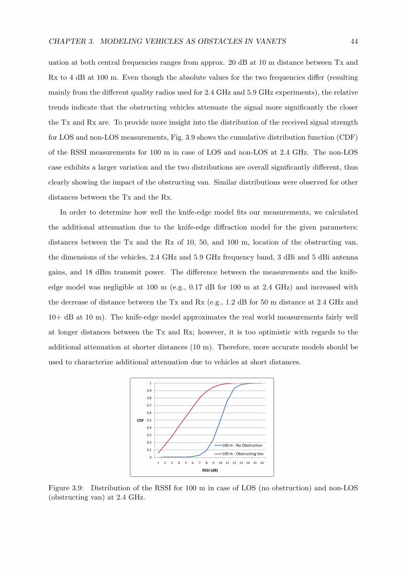
CHAPTER 3. MODELING VEHICLES AS OBSTACLES IN VANETS 44
uation at both central frequencies ranges from approx. 20 dB at 10 m distance between Tx and
Rx to 4 dB at 100 m. Even though the absolute values for the two frequencies differ (resulting
mainly from the different quality radios used for 2.4 GHz and 5.9 GHz experiments), the relative
trends indicate that the obstructing vehicles attenuate the signal more significantly the closer
the Tx and Rx are. To provide more insight into the distribution of the received signal strength
for LOS and non-LOS measurements, Fig. 3.9 shows the cumulative distribution function (CDF)
of the RSSI measurements for 100 m in case of LOS and non-LOS at 2.4 GHz. The non-LOS
case exhibits a larger variation and the two distributions are overall significantly different, thus
clearly showing the impact of the obstructing van. Similar distributions were observed for other
distances between the Tx and the Rx.
In order to determine how well the knife-edge model fits our measurements, we calculated
the additional attenuation due to the knife-edge diffraction model for the given parameters:
distances between the Tx and the Rx of 10, 50, and 100 m, location of the obstructing van,
the dimensions of the vehicles, 2.4 GHz and 5.9 GHz frequency band, 3 dBi and 5 dBi antenna
gains, and 18 dBm transmit power. The difference between the measurements and the knife-
edge model was negligible at 100 m (e.g., 0.17 dB for 100 m at 2.4 GHz) and increased with
the decrease of distance between the Tx and Rx (e.g., 1.2 dB for 50 m distance at 2.4 GHz and
10+ dB at 10 m). The knife-edge model approximates the real world measurements fairly well
at longer distances between the Tx and Rx; however, it is too optimistic with regards to the
additional attenuation at shorter distances (10 m). Therefore, more accurate models should be
used to characterize additional attenuation due to vehicles at short distances.
0
0,1
0,2
0,3
0,4
0,5
0,6
0,7
0,8
0,9
1
1 2 3 4 5 6 7 8 9 10 11 12 13 14 15 16
CDF
RSSI (dB)
100 m - No Obstruction
100 m - Obstructing Van
Figure 3.9: Distribution of the RSSI for 100 m in case of LOS (no obstruction) and non-LOS(obstructing van) at 2.4 GHz.
CHAPTER 3. MODELING VEHICLES AS OBSTACLES IN VANETS 45
3.6 Conclusions
We proposed a new model for incorporating vehicles as obstacles in VANET simulation en-
vironments. First, we analyzed the real world data collected by means of stereoscopic aerial
photography and showed that vehicles as obstacles have a significant impact on LOS obstruc-
tion in both dense and sparse vehicular networks, and should therefore be included in V2V
channel modeling. Then, based on the concepts of computational geometry, we modeled the
vehicles as three-dimensional objects that can act as LOS obstructions between other commu-
nicating vehicles. Next, we designed a mechanism for calculating additional attenuation due
to vehicles as obstacles, and we showed that the obstructing vehicles significantly decrease the
received signal power and the packet success rate. We also performed experimental measure-
ments in order to confirm the significance of the impact of obstructing vehicles on the received
signal strength. clearly indicate that vehicles as obstacles have a significant impact on signal
propagation (see Fig. 3.5 and 3.8); therefore, in order to properly model V2V communication, it
is imperative to account for vehicles as obstacles. Furthermore, the effect of vehicles as obstacles
can not be neglected even in the case of relatively sparse vehicular networks, as the analyzed
A3 highway dataset showed.
Furthermore, neglecting vehicles as obstacles in VANET simulation and modeling has pro-
found effects on the performance evaluation of upper layers of the communication stack. The
expected effects on the data link layer are twofold: a) the medium contention is overestimated in
models that do not include vehicles as obstacles in the calculation, thus potentially representing
a more pessimistic situation than the real-world with regards to contention and collision; and
b) the network reachability is bound to be overestimated, due to the fact that the signal is
considered to reach more neighbors and at a higher power than in the real world. These results
have important implications for vehicular Medium Access Control (MAC) protocol design; MAC
protocols will have to cope with an increased number of hidden vehicles due to other vehicles
obstructing them.
The algorithm behind the proposed model, even though microscopically evaluating the atten-
uation due to vehicles (i.e., calculating additional attenuation due to vehicles for each communi-
cating pair separately), remains computationally efficient, location independent, and compatible
with models that evaluate the effect of other types of obstacles. By implementing the proposed
CHAPTER 3. MODELING VEHICLES AS OBSTACLES IN VANETS 46
model in VANET simulators, significant benefits can be obtained with respect to increased
credibility of simulation results, at the expense of a relatively small computational overhead.

Chapter 4
Vehicle-to-Vehicle Channel Model
for VANET Simulations
4.1 Motivation
In the previous chapter, we proposed a model for incorporating the impact of vehicles as ob-
structions in vehicle-to-vehicle (V2V) communication. In highway environments, we showed
that vehicles are the predominant source of shadowing [16, 69]. To realistically characterize
the channel in environments where other objects have a significant impact on the signal (e.g.,
buildings and foliage in urban and suburban areas), we need to model these objects as well. To
that end, in this chapter we design a model that, apart from vehicles, also takes into account
buildings and foliage1.
Our main goal is to design a computationally manageable channel model for implementa-
tion in discrete-event packet-level Vehicular Ad Hoc Network (VANET) simulators. To better
estimate the channel conditions, we account for specific objects in the region around the com-
municating vehicles. Previous studies have shown that simplified statistical channel models
are unable to simulate VANET channels accurately [1, 2]. On the other hand, location-specific
channel models such as those based on ray-tracing [12] yield results that are in a very good
agreement with the real world. However, these models are computationally too expensive due
to prohibitive computation costs as the network grows. Another notable problem of ray-tracing
1Throughout the text, due to the lack of a more appropriate all-encompassing term, we use the term “foliage”for vegetation such as trees, bushes, shrubbery, etc.
47
CHAPTER 4. VEHICLE-TO-VEHICLE CHANNELMODEL FOR VANET SIMULATIONS48
models is the need for detailed object database (e.g., location of doors and windows on build-
ings), as well as the sensitivity to the inaccuracies of the object database, which make it difficult
to correctly predict the path of the reflecting and diffracting rays interacting with the building..
For these reasons, ray-tracing models have not been implemented in large-scale, packet-level
VANET simulators.
We aim to bridge the gap between overly simplified statistical models and computationally
expensive ray-tracing models by performing location-specific channel modeling with respect
to large objects in the vicinity of the communicating vehicles, at the same time limiting the
calculations by using only the simple representation of the objects (i.e., outlines). We use the
real-world locations and dimensions of the buildings, foliage, and vehicles to determine the line
of sight conditions for each link. To provide the baseline for the validation of our model, we
start by performing a set of experiments in different environments (highway, urban, suburban,
open space). Using the measurements, we characterize the most important factors impacting
V2V links in each of the environments, which we then use to design a more efficient and accurate
channel model. We implement spatial tree structures for efficient manipulation of geographic
data to discriminate between three different link types: line of sight (LOS), non-LOS due to
vehicles (NLOSv), and non-LOS due to static objects (NLOSb). Apart from large-scale signal
variations due to shadowing, we also calculate the small-scale effects using the information
about the number and size of the objects around the communicating vehicles. We validate our
model using the collected experimental data. The results generated by the model match the
measurements well in terms of both the large-scale effects (shadowing) as well as small-scale
(multipath). We provide the complete simulation recipe for the implementation of the model
in simulators and we implement the model in Matlab. We show that the model scales well
by simulating networks of different size, with up to tens of thousands of objects in the scene
and hundred thousand communicating pairs. Since the model requires only the locations and
outlines of the modeled objects (buildings, foliage, and vehicles), all of which are easy to obtain,
it is well suited for the implementation in discrete-event VANET simulators.
The rest of the chapter is organized as follows. The details of the experimental setup are
shown in Section 4.2. Section 4.3 explains the spatial tree structures we use to efficiently
implement the model. Section 4.4 describes the proposed channel model, along with the recipe
for implementation of the model in VANET simulators. Results validating the proposed model
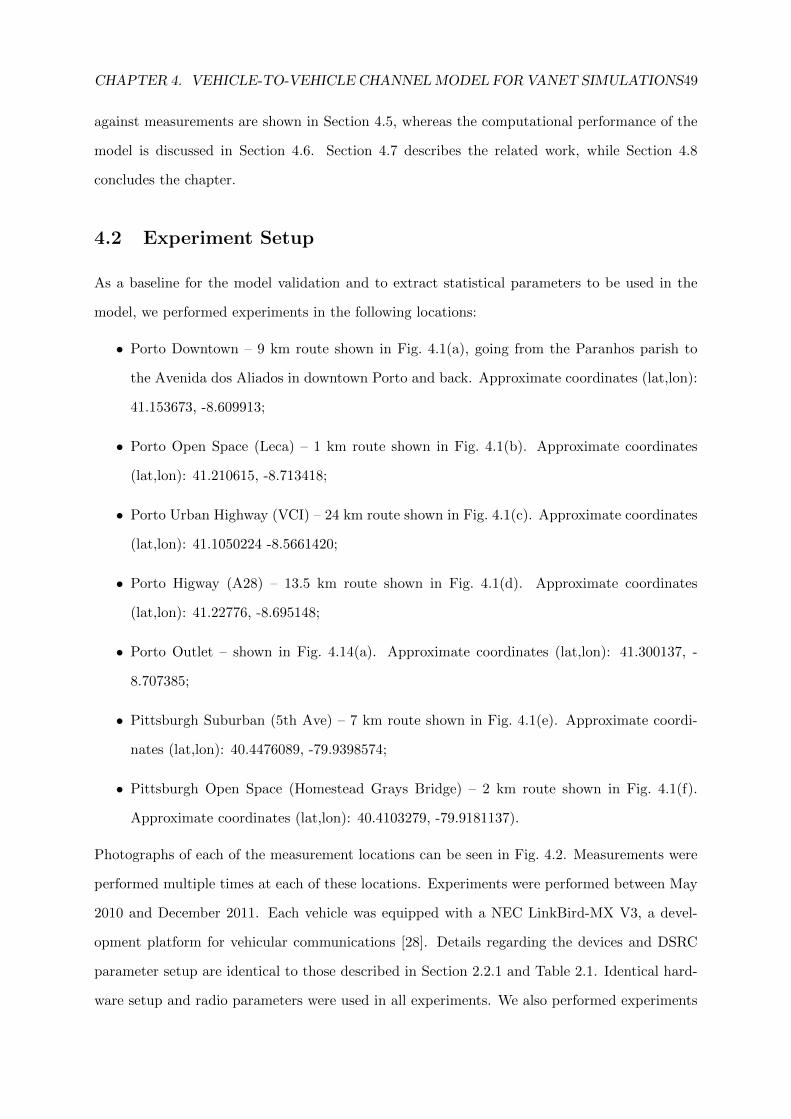
CHAPTER 4. VEHICLE-TO-VEHICLE CHANNELMODEL FOR VANET SIMULATIONS49
against measurements are shown in Section 4.5, whereas the computational performance of the
model is discussed in Section 4.6. Section 4.7 describes the related work, while Section 4.8
concludes the chapter.
4.2 Experiment Setup
As a baseline for the model validation and to extract statistical parameters to be used in the
model, we performed experiments in the following locations:
• Porto Downtown – 9 km route shown in Fig. 4.1(a), going from the Paranhos parish to
the Avenida dos Aliados in downtown Porto and back. Approximate coordinates (lat,lon):
41.153673, -8.609913;
• Porto Open Space (Leca) – 1 km route shown in Fig. 4.1(b). Approximate coordinates
(lat,lon): 41.210615, -8.713418;
• Porto Urban Highway (VCI) – 24 km route shown in Fig. 4.1(c). Approximate coordinates
(lat,lon): 41.1050224 -8.5661420;
• Porto Higway (A28) – 13.5 km route shown in Fig. 4.1(d). Approximate coordinates
(lat,lon): 41.22776, -8.695148;
• Porto Outlet – shown in Fig. 4.14(a). Approximate coordinates (lat,lon): 41.300137, -
8.707385;
• Pittsburgh Suburban (5th Ave) – 7 km route shown in Fig. 4.1(e). Approximate coordi-
nates (lat,lon): 40.4476089, -79.9398574;
• Pittsburgh Open Space (Homestead Grays Bridge) – 2 km route shown in Fig. 4.1(f).
Approximate coordinates (lat,lon): 40.4103279, -79.9181137).
Photographs of each of the measurement locations can be seen in Fig. 4.2. Measurements were
performed multiple times at each of these locations. Experiments were performed between May
2010 and December 2011. Each vehicle was equipped with a NEC LinkBird-MX V3, a devel-
opment platform for vehicular communications [28]. Details regarding the devices and DSRC
parameter setup are identical to those described in Section 2.2.1 and Table 2.1. Identical hard-
ware setup and radio parameters were used in all experiments. We also performed experiments
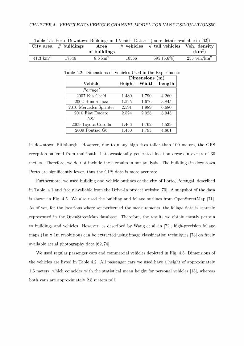
CHAPTER 4. VEHICLE-TO-VEHICLE CHANNELMODEL FOR VANET SIMULATIONS50
Table 4.1: Porto Downtown Buildings and Vehicle Dataset (more details available in [62])City area # buildings Area # vehicles # tall vehicles Veh. density
of buildings (km2)
41.3 km2 17346 8.6 km2 10566 595 (5.6%) 255 veh/km2
Table 4.2: Dimensions of Vehicles Used in the ExperimentsDimensions (m)
Vehicle Height Width Length
Portugal
2007 Kia Cee’d 1.480 1.790 4.260
2002 Honda Jazz 1.525 1.676 3.845
2010 Mercedes Sprinter 2.591 1.989 6.680
2010 Fiat Ducato 2.524 2.025 5.943
USA
2009 Toyota Corolla 1.466 1.762 4.539
2009 Pontiac G6 1.450 1.793 4.801
in downtown Pittsburgh. However, due to many high-rises taller than 100 meters, the GPS
reception suffered from multipath that occasionally generated location errors in excess of 30
meters. Therefore, we do not include these results in our analysis. The buildings in downtown
Porto are significantly lower, thus the GPS data is more accurate.
Furthermore, we used building and vehicle outlines of the city of Porto, Portugal, described
in Table. 4.1 and freely available from the Drive-In project website [70]. A snapshot of the data
is shown in Fig. 4.5. We also used the building and foliage outlines from OpenStreetMap [71].
As of yet, for the locations where we performed the measurements, the foliage data is scarcely
represented in the OpenStreetMap database. Therefore, the results we obtain mostly pertain
to buildings and vehicles. However, as described by Wang et al. in [72], high-precision foliage
maps (1m x 1m resolution) can be extracted using image classification techniques [73] on freely
available aerial photography data [62,74].
We used regular passenger cars and commercial vehicles depicted in Fig. 4.3. Dimensions of
the vehicles are listed in Table 4.2. All passenger cars we used have a height of approximately
1.5 meters, which coincides with the statistical mean height for personal vehicles [15], whereas
both vans are approximately 2.5 meters tall.
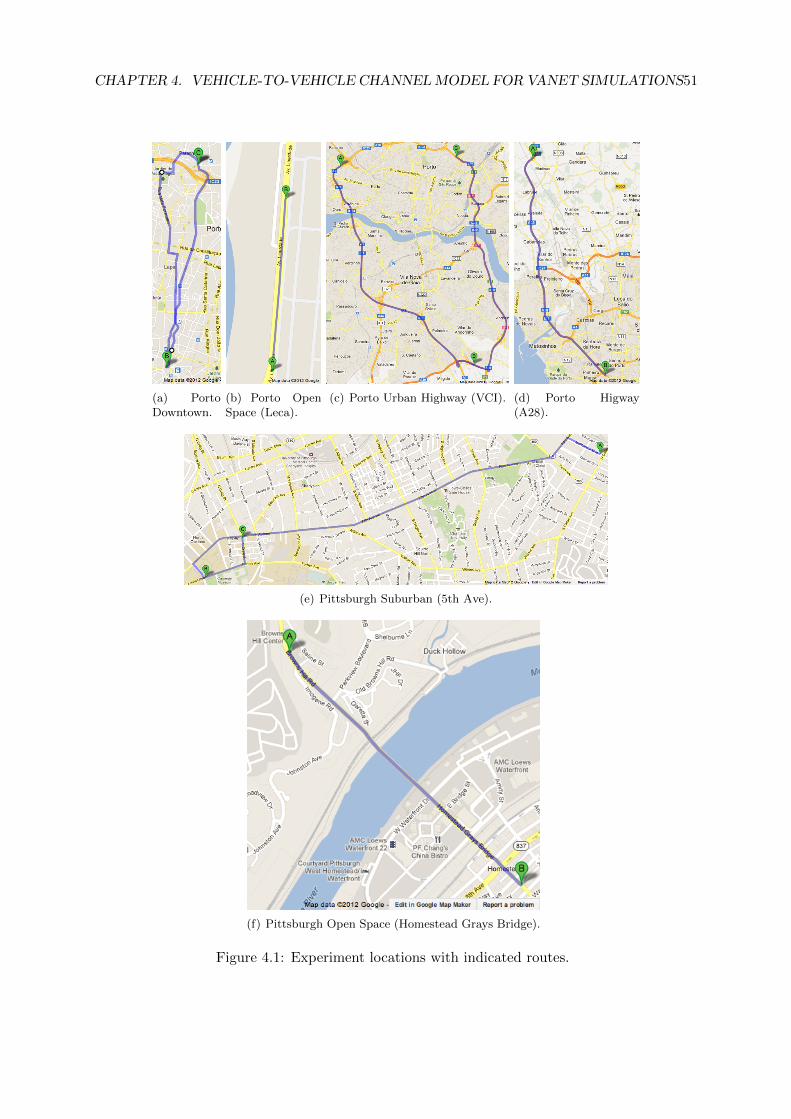
CHAPTER 4. VEHICLE-TO-VEHICLE CHANNELMODEL FOR VANET SIMULATIONS51
(a) PortoDowntown.
(b) Porto OpenSpace (Leca).
(c) Porto Urban Highway (VCI). (d) Porto Higway(A28).
(e) Pittsburgh Suburban (5th Ave).
(f) Pittsburgh Open Space (Homestead Grays Bridge).
Figure 4.1: Experiment locations with indicated routes.
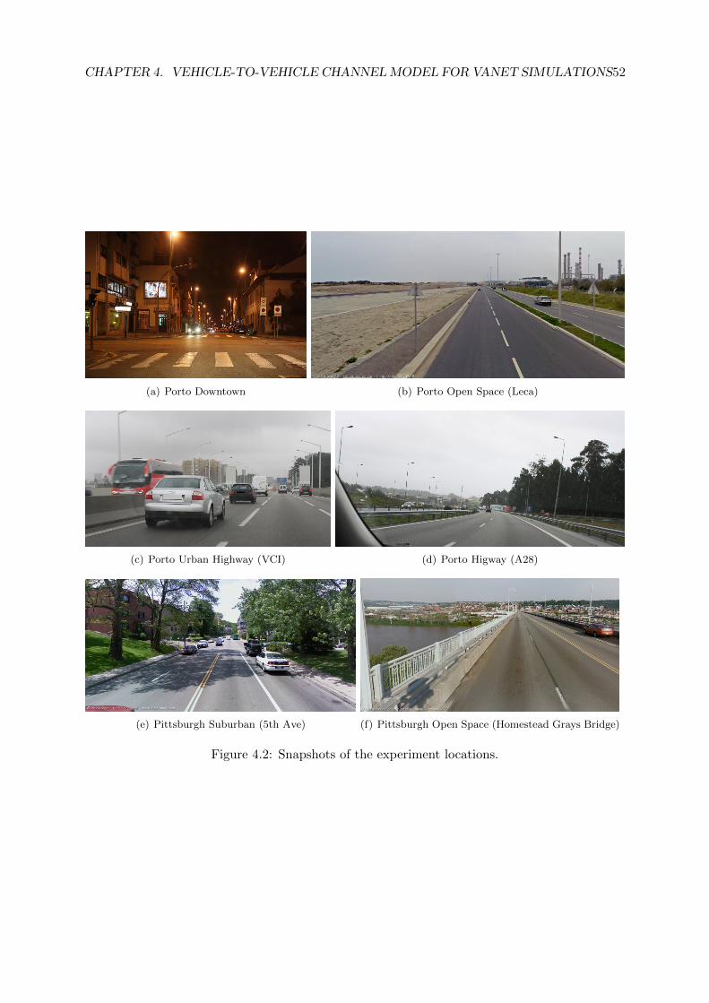
CHAPTER 4. VEHICLE-TO-VEHICLE CHANNELMODEL FOR VANET SIMULATIONS52
(a) Porto Downtown (b) Porto Open Space (Leca)
(c) Porto Urban Highway (VCI) (d) Porto Higway (A28)
(e) Pittsburgh Suburban (5th Ave) (f) Pittsburgh Open Space (Homestead Grays Bridge)
Figure 4.2: Snapshots of the experiment locations.
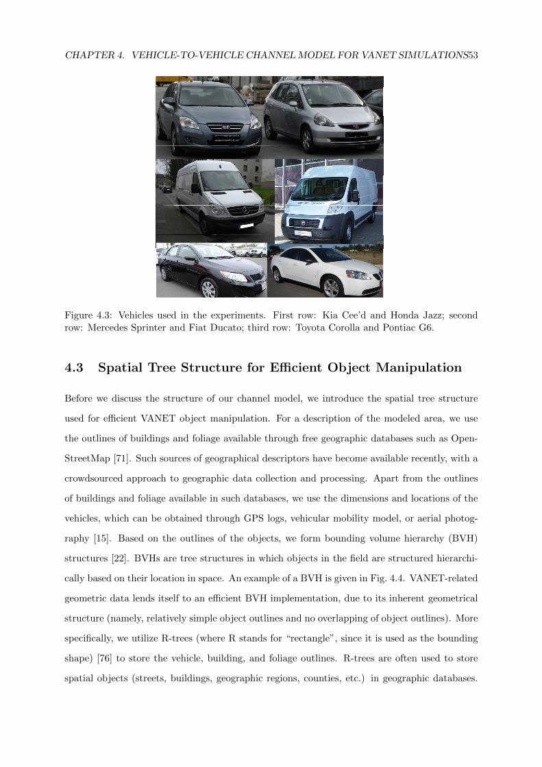
CHAPTER 4. VEHICLE-TO-VEHICLE CHANNELMODEL FOR VANET SIMULATIONS53
3
Friday, October 14, 11
Figure 4.3: Vehicles used in the experiments. First row: Kia Cee’d and Honda Jazz; secondrow: Mercedes Sprinter and Fiat Ducato; third row: Toyota Corolla and Pontiac G6.
4.3 Spatial Tree Structure for Efficient Object Manipulation
Before we discuss the structure of our channel model, we introduce the spatial tree structure
used for efficient VANET object manipulation. For a description of the modeled area, we use
the outlines of buildings and foliage available through free geographic databases such as Open-
StreetMap [71]. Such sources of geographical descriptors have become available recently, with a
crowdsourced approach to geographic data collection and processing. Apart from the outlines
of buildings and foliage available in such databases, we use the dimensions and locations of the
vehicles, which can be obtained through GPS logs, vehicular mobility model, or aerial photog-
raphy [15]. Based on the outlines of the objects, we form bounding volume hierarchy (BVH)
structures [22]. BVHs are tree structures in which objects in the field are structured hierarchi-
cally based on their location in space. An example of a BVH is given in Fig. 4.4. VANET-related
geometric data lends itself to an efficient BVH implementation, due to its inherent geometrical
structure (namely, relatively simple object outlines and no overlapping of object outlines). More
specifically, we utilize R-trees (where R stands for “rectangle”, since it is used as the bounding
shape) [76] to store the vehicle, building, and foliage outlines. R-trees are often used to store
spatial objects (streets, buildings, geographic regions, counties, etc.) in geographic databases.
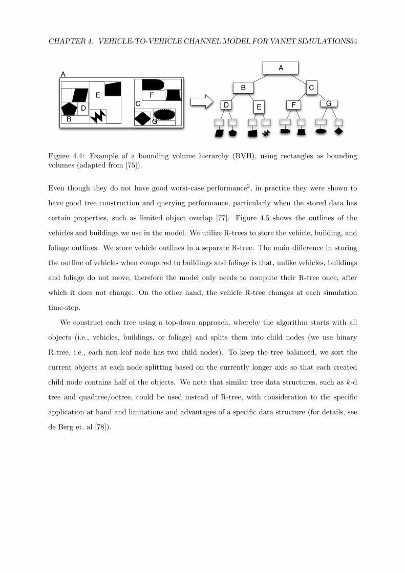
CHAPTER 4. VEHICLE-TO-VEHICLE CHANNELMODEL FOR VANET SIMULATIONS54
A
B
CD
E F
G
A
B C
D E F G
Figure 4.4: Example of a bounding volume hierarchy (BVH), using rectangles as boundingvolumes (adapted from [75]).
Even though they do not have good worst-case performance2, in practice they were shown to
have good tree construction and querying performance, particularly when the stored data has
certain properties, such as limited object overlap [77]. Figure 4.5 shows the outlines of the
vehicles and buildings we use in the model. We utilize R-trees to store the vehicle, building, and
foliage outlines. We store vehicle outlines in a separate R-tree. The main difference in storing
the outline of vehicles when compared to buildings and foliage is that, unlike vehicles, buildings
and foliage do not move, therefore the model only needs to compute their R-tree once, after
which it does not change. On the other hand, the vehicle R-tree changes at each simulation
time-step.
We construct each tree using a top-down approach, whereby the algorithm starts with all
objects (i.e., vehicles, buildings, or foliage) and splits them into child nodes (we use binary
R-tree, i.e., each non-leaf node has two child nodes). To keep the tree balanced, we sort the
current objects at each node splitting based on the currently longer axis so that each created
child node contains half of the objects. We note that similar tree data structures, such as k -d
tree and quadtree/octree, could be used instead of R-tree, with consideration to the specific
application at hand and limitations and advantages of a specific data structure (for details, see
de Berg et. al [78]).
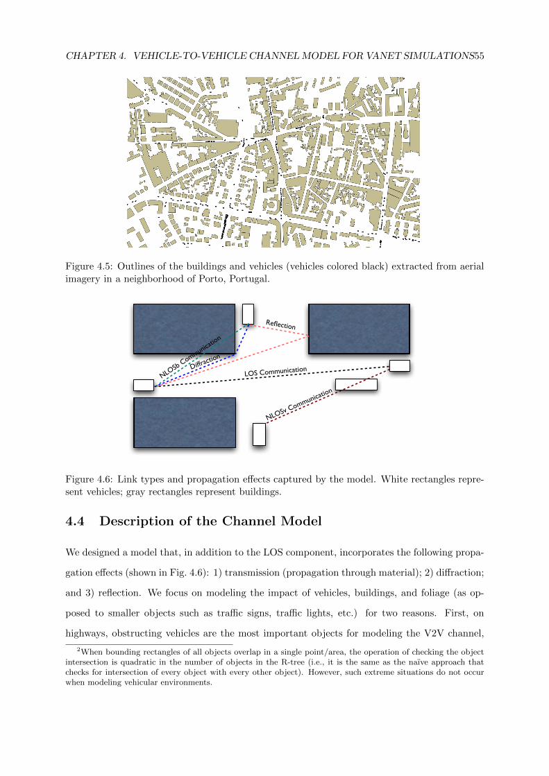
CHAPTER 4. VEHICLE-TO-VEHICLE CHANNELMODEL FOR VANET SIMULATIONS55
Figure 4.5: Outlines of the buildings and vehicles (vehicles colored black) extracted from aerialimagery in a neighborhood of Porto, Portugal.
NLOSv Communication
Diffraction
Reflection
LOS CommunicationNLO
Sb Communi
cation
Tuesday, November 27, 12
Figure 4.6: Link types and propagation effects captured by the model. White rectangles repre-sent vehicles; gray rectangles represent buildings.
4.4 Description of the Channel Model
We designed a model that, in addition to the LOS component, incorporates the following propa-
gation effects (shown in Fig. 4.6): 1) transmission (propagation through material); 2) diffraction;
and 3) reflection. We focus on modeling the impact of vehicles, buildings, and foliage (as op-
posed to smaller objects such as traffic signs, traffic lights, etc.) for two reasons. First, on
highways, obstructing vehicles are the most important objects for modeling the V2V channel,
2When bounding rectangles of all objects overlap in a single point/area, the operation of checking the objectintersection is quadratic in the number of objects in the R-tree (i.e., it is the same as the naıve approach thatchecks for intersection of every object with every other object). However, such extreme situations do not occurwhen modeling vehicular environments.
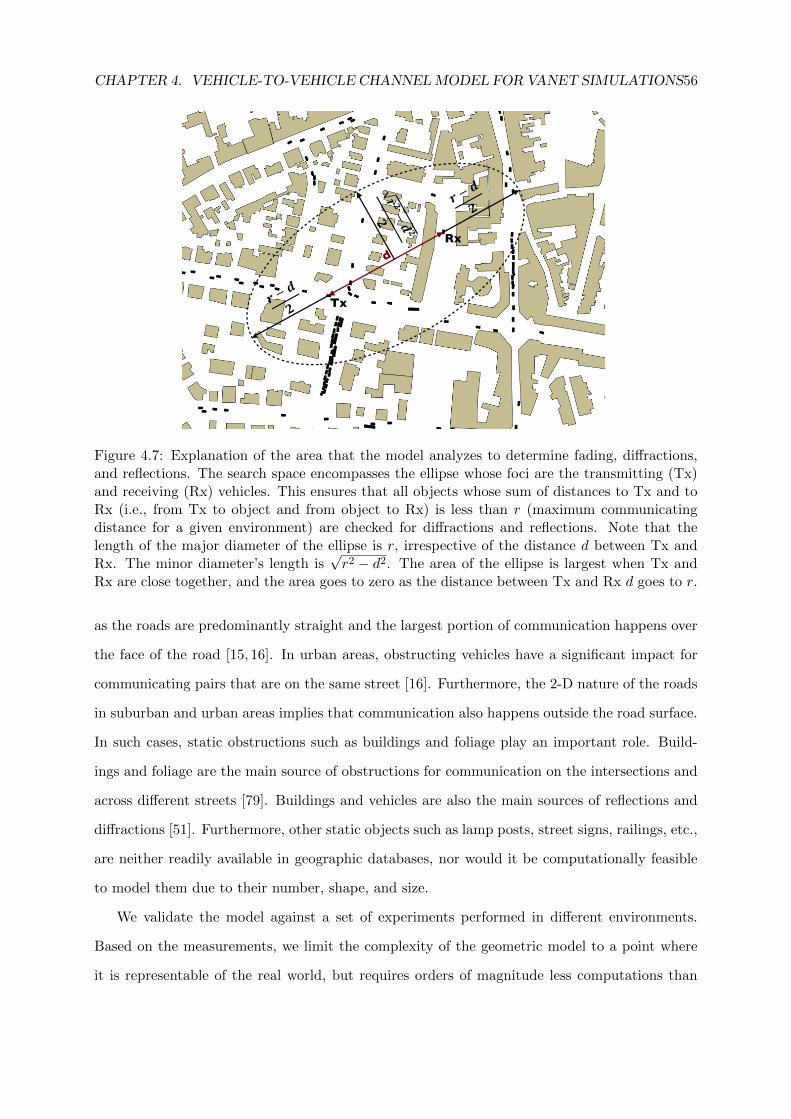
CHAPTER 4. VEHICLE-TO-VEHICLE CHANNELMODEL FOR VANET SIMULATIONS56
Tx
Rx
d
! !−! !!
!
!− !!!
!− !!!
Monday, October 24, 11
Figure 4.7: Explanation of the area that the model analyzes to determine fading, diffractions,and reflections. The search space encompasses the ellipse whose foci are the transmitting (Tx)and receiving (Rx) vehicles. This ensures that all objects whose sum of distances to Tx and toRx (i.e., from Tx to object and from object to Rx) is less than r (maximum communicatingdistance for a given environment) are checked for diffractions and reflections. Note that thelength of the major diameter of the ellipse is r, irrespective of the distance d between Tx andRx. The minor diameter’s length is
√r2 − d2. The area of the ellipse is largest when Tx and
Rx are close together, and the area goes to zero as the distance between Tx and Rx d goes to r.
as the roads are predominantly straight and the largest portion of communication happens over
the face of the road [15, 16]. In urban areas, obstructing vehicles have a significant impact for
communicating pairs that are on the same street [16]. Furthermore, the 2-D nature of the roads
in suburban and urban areas implies that communication also happens outside the road surface.
In such cases, static obstructions such as buildings and foliage play an important role. Build-
ings and foliage are the main source of obstructions for communication on the intersections and
across different streets [79]. Buildings and vehicles are also the main sources of reflections and
diffractions [51]. Furthermore, other static objects such as lamp posts, street signs, railings, etc.,
are neither readily available in geographic databases, nor would it be computationally feasible
to model them due to their number, shape, and size.
We validate the model against a set of experiments performed in different environments.
Based on the measurements, we limit the complexity of the geometric model to a point where
it is representable of the real world, but requires orders of magnitude less computations than
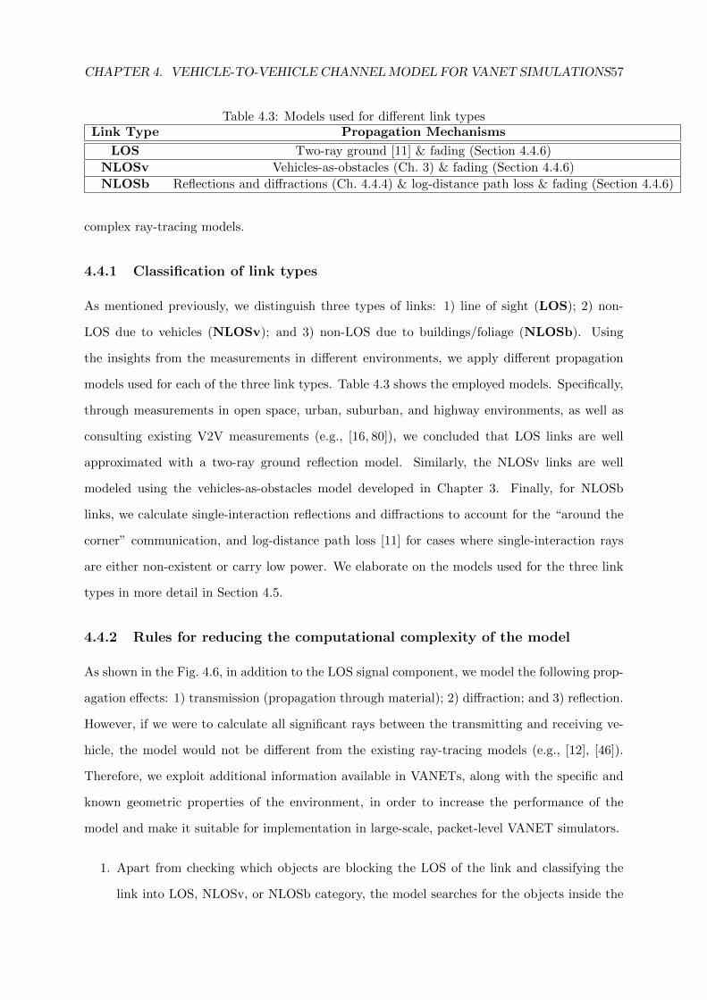
CHAPTER 4. VEHICLE-TO-VEHICLE CHANNELMODEL FOR VANET SIMULATIONS57
Table 4.3: Models used for different link typesLink Type Propagation Mechanisms
LOS Two-ray ground [11] & fading (Section 4.4.6)
NLOSv Vehicles-as-obstacles (Ch. 3) & fading (Section 4.4.6)
NLOSb Reflections and diffractions (Ch. 4.4.4) & log-distance path loss & fading (Section 4.4.6)
complex ray-tracing models.
4.4.1 Classification of link types
As mentioned previously, we distinguish three types of links: 1) line of sight (LOS); 2) non-
LOS due to vehicles (NLOSv); and 3) non-LOS due to buildings/foliage (NLOSb). Using
the insights from the measurements in different environments, we apply different propagation
models used for each of the three link types. Table 4.3 shows the employed models. Specifically,
through measurements in open space, urban, suburban, and highway environments, as well as
consulting existing V2V measurements (e.g., [16, 80]), we concluded that LOS links are well
approximated with a two-ray ground reflection model. Similarly, the NLOSv links are well
modeled using the vehicles-as-obstacles model developed in Chapter 3. Finally, for NLOSb
links, we calculate single-interaction reflections and diffractions to account for the “around the
corner” communication, and log-distance path loss [11] for cases where single-interaction rays
are either non-existent or carry low power. We elaborate on the models used for the three link
types in more detail in Section 4.5.
4.4.2 Rules for reducing the computational complexity of the model
As shown in the Fig. 4.6, in addition to the LOS signal component, we model the following prop-
agation effects: 1) transmission (propagation through material); 2) diffraction; and 3) reflection.
However, if we were to calculate all significant rays between the transmitting and receiving ve-
hicle, the model would not be different from the existing ray-tracing models (e.g., [12], [46]).
Therefore, we exploit additional information available in VANETs, along with the specific and
known geometric properties of the environment, in order to increase the performance of the
model and make it suitable for implementation in large-scale, packet-level VANET simulators.
1. Apart from checking which objects are blocking the LOS of the link and classifying the
link into LOS, NLOSv, or NLOSb category, the model searches for the objects inside the
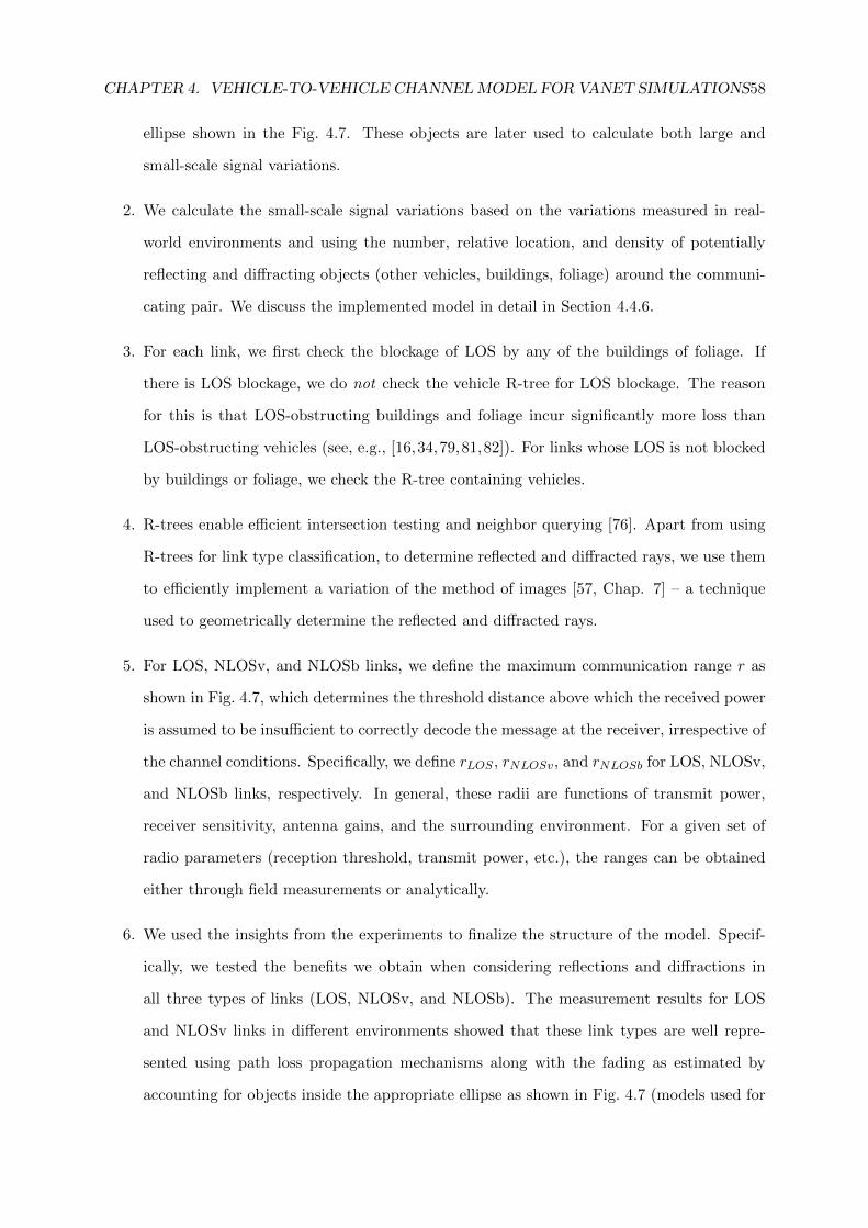
CHAPTER 4. VEHICLE-TO-VEHICLE CHANNELMODEL FOR VANET SIMULATIONS58
ellipse shown in the Fig. 4.7. These objects are later used to calculate both large and
small-scale signal variations.
2. We calculate the small-scale signal variations based on the variations measured in real-
world environments and using the number, relative location, and density of potentially
reflecting and diffracting objects (other vehicles, buildings, foliage) around the communi-
cating pair. We discuss the implemented model in detail in Section 4.4.6.
3. For each link, we first check the blockage of LOS by any of the buildings of foliage. If
there is LOS blockage, we do not check the vehicle R-tree for LOS blockage. The reason
for this is that LOS-obstructing buildings and foliage incur significantly more loss than
LOS-obstructing vehicles (see, e.g., [16,34,79,81,82]). For links whose LOS is not blocked
by buildings or foliage, we check the R-tree containing vehicles.
4. R-trees enable efficient intersection testing and neighbor querying [76]. Apart from using
R-trees for link type classification, to determine reflected and diffracted rays, we use them
to efficiently implement a variation of the method of images [57, Chap. 7] – a technique
used to geometrically determine the reflected and diffracted rays.
5. For LOS, NLOSv, and NLOSb links, we define the maximum communication range r as
shown in Fig. 4.7, which determines the threshold distance above which the received power
is assumed to be insufficient to correctly decode the message at the receiver, irrespective of
the channel conditions. Specifically, we define rLOS , rNLOSv, and rNLOSb for LOS, NLOSv,
and NLOSb links, respectively. In general, these radii are functions of transmit power,
receiver sensitivity, antenna gains, and the surrounding environment. For a given set of
radio parameters (reception threshold, transmit power, etc.), the ranges can be obtained
either through field measurements or analytically.
6. We used the insights from the experiments to finalize the structure of the model. Specif-
ically, we tested the benefits we obtain when considering reflections and diffractions in
all three types of links (LOS, NLOSv, and NLOSb). The measurement results for LOS
and NLOSv links in different environments showed that these link types are well repre-
sented using path loss propagation mechanisms along with the fading as estimated by
accounting for objects inside the appropriate ellipse as shown in Fig. 4.7 (models used for
CHAPTER 4. VEHICLE-TO-VEHICLE CHANNELMODEL FOR VANET SIMULATIONS59
link types are shown in Table 4.3, whereas details on the match between the model and
measurements for these links are shown in Section 4.5). Furthermore, adding reflections
and diffractions resulted in minimal benefits in terms of accuracy, while incurring a high
computational overhead. On the other hand, for NLOSb links, reflected and diffracted
rays account for a significant portion of the received power. Therefore, we explicitly model
the single interaction reflections and diffractions for NLOSb links only.
4.4.3 Transmission through Foliage
For foliage, we use the attenuation-through-transmission model based on the measurements
described in [82–85]. Specifically, we use the empirically-derived formulation from [83] where
attenuation for deciduous trees is calculated per meter of transmission using
MEL = 0.79f0.61, (4.1)
where MEL is mean excess loss per meter of transmission through trees and f is frequency
in GHz [85]. For DSRC frequency centered at 5.9 GHz, this results in attenuation of 2.3 dB
per meter of transmission through trees, which is in line with the measurement results in the
5.85 GHz band reported in [82]. Similar calculations can be performed for coniferous trees as
well as for seasonal changes when trees are not in full foliage [83]. Decision on which kind of
trees to model (deciduous or coniferous) and the level of foliage (e.g., due to the time of the year)
needs to be determined for the location where the simulations are carried out. Furthermore,
geographic databases such as OpenStreetMap have tagging systems that allow for specification
of such characterstics [71]; provided that the different types of vegetation are tagged properly,
they can be distinguished and modeled accordingly. Finally, we do not model any reflections or
diffractions off foliage (i.e., only transmission attenuation is accounted for); rather, we implicitly
encompass their scattering effects in the fading calculations.
4.4.4 Combining multiple paths: E-field and received power calculations
Once all contributing rays (LOS, reflected, diffracted, and transmitted) have been obtained, we
calculate their contributions in terms of the E-field and the received power for each link. We
CHAPTER 4. VEHICLE-TO-VEHICLE CHANNELMODEL FOR VANET SIMULATIONS60
obtain the resultant E-field envelope as follows [11, Chap. 3.]:
|ETOT | = |ELOS +∑j
EReflj +∑k
Ediffrk |, (4.2)
where ELOS , ERefl, and Ediffr are E-fieds of line or sight, reflected, and diffracted rays, respec-
tively. Expanding eq. 4.2, we get
ETOT =E0d0
dLOScos
(ωc
(t− dLOS
c
))+∑j
RjE0d0
djcos
(ωc
(t− dj
c
))+∑k
DkE0d0
dkcos
(ωc
(t− dk
c
)),
(4.3)
where E0d0dLOS
is the envelope E-field at a reference distance d0, ωc is the angular frequency
(ωc = 2πf), t is the time at which the E-field is evaluated, dx represents distance traversed by ray
x, Rj is the reflection coefficient of reflected ray j, Dk is the diffraction coefficient of diffracted
ray k. When the originating medium is free space, the reflected coefficient R is calculated as
follows for vertical and horizontal polarization, respectively [11, Chap. 3.]:
R|| =−εr sin θi +
√εr − cos2 θi
εr sin θi +√εr − cos2 θi
(4.4)
and
R⊥ =sin θi −
√εr − cos2 θi
sin θi +√εr − cos2 θi
, (4.5)
where θi is the incident angle, and εr is the relative permittivity of the material.
Regarding diffractions, we do not calculate the diffraction coefficient directly; we approximate
the E-field for diffracted rays using the knife-edge model [56]. However, the model contains all
the geographical information to calculate the diffraction parameter for single diffractions using
uniform theory of diffraction (UTD) [86].
The ensuing received power Pr (in watts), assuming unit antenna gains, is calculated as
follows:
Pr =|ETOT |2λ2
480π2, (4.6)
where λ is the wavelength. Note that Pr accounts for the slow fading signal component of LOS
CHAPTER 4. VEHICLE-TO-VEHICLE CHANNELMODEL FOR VANET SIMULATIONS61
links, whereas for NLOSv and NLOSb links there are also contributions in terms of multipath
generated by multiple diffractions around vehicles in case of NLOSv (horizontal and vertical
multiple knife-edge diffractions) and single interaction reflections and diffractions in case of
NLOSb.
Furthermore, in cases where the accuracy of the geographic database is not sufficiently high
for correct calculation of the phase shift – this might often be the case for DSRC systems,
since the wavelength is approximately 5 cm, thus requiring centimeter-grade database precision
– the phase shift component in the eq. 4.3 for different incoming rays can be approximated
using a distribution that represents the given environment well (e.g., uniform in case of isotropic
scattering or based on the predominant angles of arrival in case of non-isotropic scattering [50,
87]).
4.4.5 Practical considerations for different link types and propagation mech-
anisms
LOS communication
For LOS links, we implement the complete two-ray ground reflection model given by the following
equation [11, Chap. 3]:
ETOT =E0d0
dLOScos
(ωc
(t− dLOS
c
))+Rground
E0d0
dgroundcos
(ωc
(t− dground
c
)), (4.7)
where the reflection coefficient Rground and distance dground for the ground-reflected ray are
calculated according to the exact antenna heights (i.e., we do not assume that the distance
between transmitter and receiver is large compared to heights of the vehicles, as is often done
in simulators [19], [20]). As will become apparent from our results (Section 4.5), using the exact
height of the antennas is important, since even a 10 cm difference in height of either Tx or Rx
results in significantly different interference relationship between the LOS and ground-reflected
ray.
In calculating Rground, we model the relative permittivity εr to obtain the “effective” range
of the reflection coefficient for the road. It was pointed out in [88] that the idealized two-ray
model is an approximation of the actual V2V channel, since the reflection coefficient is affected
CHAPTER 4. VEHICLE-TO-VEHICLE CHANNELMODEL FOR VANET SIMULATIONS62
by the antenna location, diffraction over the vehicle roof below antenna, and the roughness of
the road, among other. Therefore, we set the er value used to generate the LOS results to 1.003,
as this value minimized the mean square error for Leca dataset (see Section 4.5). Then, we
use the same er value for LOS links in all environments. Similar concept of effective reflection
coefficient range calculation was used in the following studies: [89], [80], and [88].
Reflections
With respect to the reflection coefficients off building walls, we apply similar reasoning on the
“effective” range of reflection coefficients as with the two-ray ground reflection model. We match
the reflection coefficient distribution to the values empirically derived in [90], where the authors
extract the reflection coefficients for brick building walls from controlled measurements. In
the measurement locations, walls of reflecting buildings were predominantly made of brick and
concrete.
The reflections are calculated from buildings and from vehicles. Since all buildings are
significantly taller than any vehicle, any building can reflect the signal for any communicating
pair. On the other hand, in order to be a reflector, a vehicle needs to be taller than both
communicating vehicles’ antennas, since otherwise the reflected ray does not exist. In practice,
this means that tall vehicles are predominant among reflecting vehicles. Furthermore, as can be
seen in Fig. 4.8, tall vehicles are more likely to block reflections coming off the building walls or
other vehicles, whereas short vehicles are less likely to do so, since their height is often shorter
than the height of the line between the communicating antennas discounted for the 60% of the
first Fresnel zone.
Diffractions
For building diffractions, we use the same multiple knife-edge method on the building corners
that we used for vehicle diffraction in Chapter 3 (eq. 3.8). The difference is that in the case
of buildings, the only diffraction in the horizontal plane is accounted for (we assume that the
buildings are too tall for diffraction over the rooftops), whereas in case of vehicles, the diffraction
is calculated for both the vertical plane (i.e., over the vehicle roofs) and the horizontal plane
(on the sides of the vehicles). In all cases, we perform the multiple knife-edge diffraction as
described in [56].
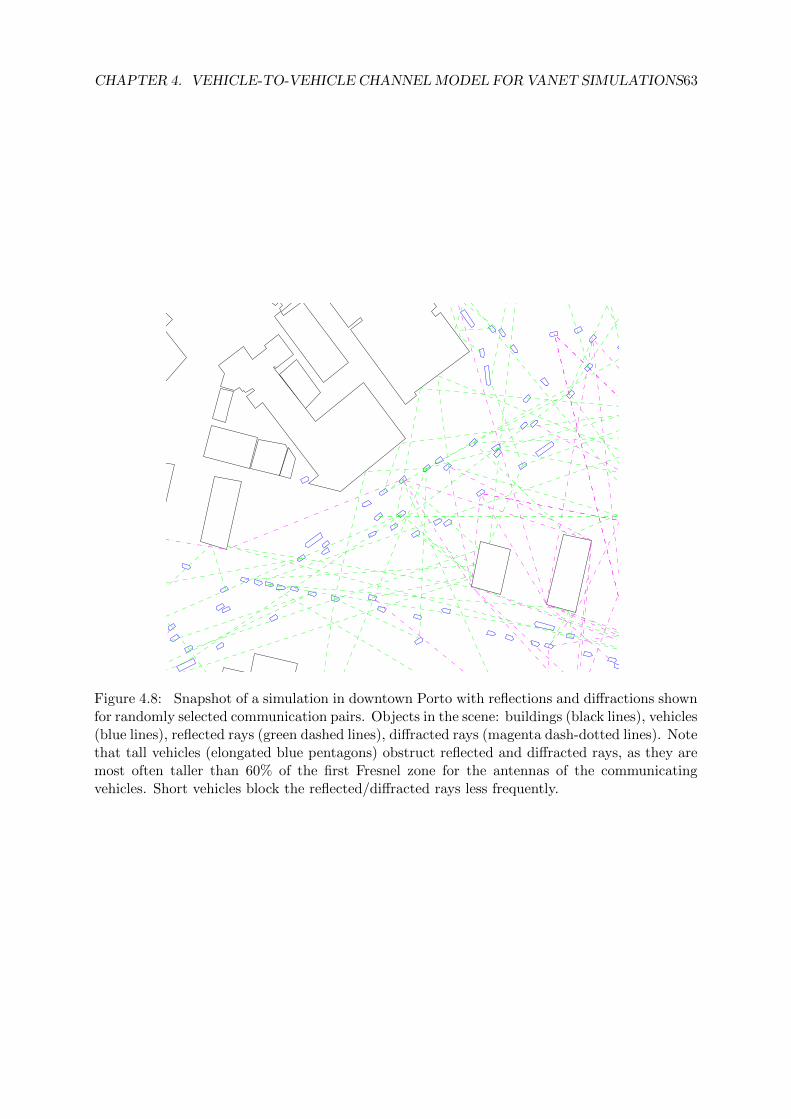
CHAPTER 4. VEHICLE-TO-VEHICLE CHANNELMODEL FOR VANET SIMULATIONS63
5.297 5.2975 5.298 5.2985 5.299 5.2995 5.3
Figure 4.8: Snapshot of a simulation in downtown Porto with reflections and diffractions shownfor randomly selected communication pairs. Objects in the scene: buildings (black lines), vehicles(blue lines), reflected rays (green dashed lines), diffracted rays (magenta dash-dotted lines). Notethat tall vehicles (elongated blue pentagons) obstruct reflected and diffracted rays, as they aremost often taller than 60% of the first Fresnel zone for the antennas of the communicatingvehicles. Short vehicles block the reflected/diffracted rays less frequently.
CHAPTER 4. VEHICLE-TO-VEHICLE CHANNELMODEL FOR VANET SIMULATIONS64
Log-distance path loss in deep-fade areas
Reflections and diffractions off buildings and vehicles are used for NLOSb links. We limit the
calculation of diffracted and reflected rays to single-interaction (single-bounce) rays, except for
multiple diffraction due to vehicles. It was recently shown by Abbas et al. in [91] that single-
interaction reflections and diffractions are most often the dominating propagation mechanisms in
the absence of LOS. The authors conclude that “single-bounce reflections with static objects e.g.,
buildings, roadsigns, and streetlights, often are the dominating propagation mechanisms in the
absence of line of sight whereas the reflections from other vehicles contribute little unless these
vehicles are tall enough.” Similar findings are reported by Paier et al. in [92]. By determining
the LOS conditions and modeling LOS and single-interaction rays, we aim to design a model
that accounts for the most important rays, at the same time keeping the computational load
manageable3.
However, communicating pairs that are not located on the same street or adjacent orthogonal
streets (e.g., vehicles in parallel streets with contiguous buildings between the streets or vehicles
several streets apart) most often do not have strong single-interaction reflected or diffracted rays,
but are still occasionally able to communicate. For such communicating pairs, multiple interac-
tion reflections and scattering are the dominant contributors of the power at the receiver [57];
calculating such rays incurs prohibitively high computations and a geographical database with
a high level of detail. Furthermore, our measurement results and those reported in similar stud-
ies (e.g., [16, 81, 93, 94]) show that communication range in NLOSb (i.e., building-obstructed)
conditions using DSRC-enabled radios operating in the 5.9 GHz frequency band is limited to
approximately 200 meters, even with the maximum transmit power. Thus, in order to avoid
costly geometric computations which often yield power levels below reception threshold, at the
same time allowing for communication in deeply faded areas, we determine the received power
as follows. We calculate the received power using both the single-interaction diffractions and
reflections through the described model and using the log-distance path loss model [57]. We use
the maximum received power of the two. The log-distance path loss PL (in dB) for distance d
3The model is easily extensible to (recursively) account for the higher order interactions, however at a pro-hibitively increasing computational cost. Furthermore, a more detailed geographical database is required in orderto model multiple interaction rays correctly.
CHAPTER 4. VEHICLE-TO-VEHICLE CHANNELMODEL FOR VANET SIMULATIONS65
is given by [57]
PL(d) = PL(d0) + 10γ log10
(d
d0
), (4.8)
where γ is the path loss exponent and PL(d0) is the path loss at a reference distance d0. For
the log-distance path loss model, the received power PrPL (in dB) at a distance d is given by
PrPL(d) = Pt − PL(d), (4.9)
where Pt is the transmitted power in dB (where Pt encompasses the transmit and receive
antenna gains).
In the simulations, we used γ=2.9, which we extracted from the Porto urban dataset for
the NLOSb conditions where there were no significant single-interaction reflections/diffractions.
Previous studies reported similar values: γ=2.9 by Durgin et. al in [82] (NLOSb environment),
2.3 ≤ γ ≤ 2.75 by Cheng et al. in [24] (suburban environment), and 2.44 ≤ γ ≤ 3.39 by
Paschalidis et al. in [95] (urban environment – various LOS conditions). Therefore, for NLOSb
links, we determine the received power as the maximum of the received power calculated by the
implemented model (using eq. 4.6 in dB) and the log-distance path loss (eq. 4.9):
PrNLOSb = max(Pr, PrPL). (4.10)
4.4.6 Small-scale signal variations
The model described above captures signal variations at different scales for different link cat-
egories (LOS, NLOSv, and NLOSb). For LOS links, the model accounts for large-scale signal
variation due to distance and ground-reflection. NLOSv and NLOSb links, on the other hand,
are by definition shadowed, albeit at different levels of obstruction within each category (in case
of NLOSv, a small or a large blocking vehicle, or one or more vehicles; in case of NLOSb, deep or
slight building obstruction). Thus, for NLOSv and NLOSb links, the variation captured by the
proposed model accounts for shadowing variation as well as part of fast fading as follows. For
NLOSv links, multiple diffraction paths around vehicles are accounted for (i.e., one path over
the vehicle roofs and two potential paths on the sides of the vehicles). For NLOSb links, the
multipath is partially accounted for by calculating the single-interaction reflections and diffrac-
tions. Therefore, the model accounts for the most significant rays in case of all three types of
CHAPTER 4. VEHICLE-TO-VEHICLE CHANNELMODEL FOR VANET SIMULATIONS66
links (LOS, NLOSv, and NLOSb). To account for additional (smaller scale) signal variation
inherent in V2V communication (e.g., due to effects such as scattering and higher order diffrac-
tions and reflections), using the insights obtained through experiments we designed a small-scale
signal variation model that captures the richness of the propagation environment surrounding
the communicating pair.
We first characterize the small-scale signal variations in the collected measurements; using
the insights from the measurements, we design a simple model that complements the previously
described components of the model that deal with large-scale signal variations.
Small-scale variations in the experimental datasets
We used the collected measurements to characterize small-scale variation in different LOS con-
ditions, environments, and with different levels of vehicular traffic (i.e., temporal variation). For
each collected measurement, we separate the data into LOS, NLOSv, and NLOSb category using
the video recorded during the experiments. Then, we divide the collected data into two-meter
distance bins. We selected two meter bins because we assume that the two meter window is
small enough not to incur significant distance-related path loss dependence, at the same time
containing enough data points to allow for a meaningful statistical characterization. Figure 4.9
shows the distribution of received power for two-meter distance bins. For the LOS datasets, the
normal distribution seems to fit the data reasonably well, with a better fit for the open space
environment LOS data (Fig. 4.9(a)) than the urban LOS data (Fig. 4.9(b)) due to the richer
reflection environment in the case of the latter. Normal fit for the NLOSv and NLOSb data is
less accurate due to the variety of conditions that are encompassed by the data (e.g., different
number of obstructing vehicles in case of NLOSv, deep or slight building obstruction in case
of NLOSb). Based on the measured data, we elect to use normal distribution to describe the
small-scale variation process in all three LOS conditions4. Therefore, the empirically determined
small-scale variation is a zero-mean normal distribution N(0, σ) (normal in dB; log-normal in
terms of power in Watts).
4This is in line with the results reported by recent V2V experimental studies described in [81] and [96].
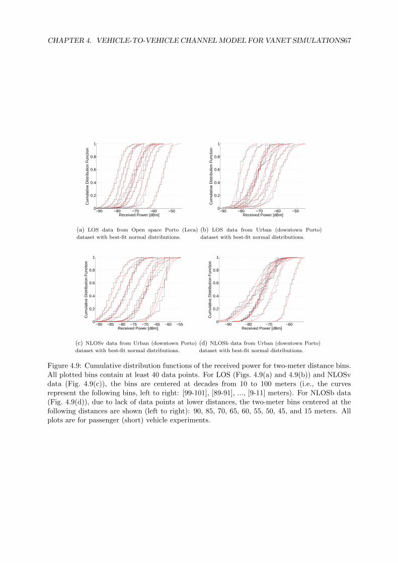
CHAPTER 4. VEHICLE-TO-VEHICLE CHANNELMODEL FOR VANET SIMULATIONS67
−90 −80 −70 −60 −500
0.2
0.4
0.6
0.8
1
Received Power [dBm]
Cum
ulat
ive
Dis
trib
utio
n F
unct
ion
(a) LOS data from Open space Porto (Leca)
dataset with best-fit normal distributions.
−90 −80 −70 −60 −500
0.2
0.4
0.6
0.8
1
Received Power [dBm]C
umul
ativ
e D
istr
ibut
ion
Fun
ctio
n
(b) LOS data from Urban (downtown Porto)
dataset with best-fit normal distributions.
−90 −85 −80 −75 −70 −65 −60 −550
0.2
0.4
0.6
0.8
1
Received Power [dBm]
Cum
ulat
ive
Dis
trib
utio
n F
unct
ion
(c) NLOSv data from Urban (downtown Porto)
dataset with best-fit normal distributions.
−90 −80 −70 −600
0.2
0.4
0.6
0.8
1
Received Power [dBm]
Cum
ulat
ive
Dis
trib
utio
n F
unct
ion
(d) NLOSb data from Urban (downtown Porto)
dataset with best-fit normal distributions.
Figure 4.9: Cumulative distribution functions of the received power for two-meter distance bins.All plotted bins contain at least 40 data points. For LOS (Figs. 4.9(a) and 4.9(b)) and NLOSvdata (Fig. 4.9(c)), the bins are centered at decades from 10 to 100 meters (i.e., the curvesrepresent the following bins, left to right: [99-101], [89-91], ..., [9-11] meters). For NLOSb data(Fig. 4.9(d)), due to lack of data points at lower distances, the two-meter bins centered at thefollowing distances are shown (left to right): 90, 85, 70, 65, 60, 55, 50, 45, and 15 meters. Allplots are for passenger (short) vehicle experiments.
CHAPTER 4. VEHICLE-TO-VEHICLE CHANNELMODEL FOR VANET SIMULATIONS68
Accounting for additional small-scale signal variation
Apart from establishing the distribution of signal variation, we also need to determine its pa-
rameter – i.e., the standard deviation σ of the normal distribution – since different environments
and LOS conditions experience different levels of signal variation, as shown in Fig. 4.9. There-
fore, we implement a simple model that accounts for the additional small-scale fading due to
the objects in the area around the communicating pair as follows. Using the communication
ellipse for each pair as explained in Fig. 4.7, we count the number of vehicles and sum the area
of static objects in the ellipse. We chose the area of the static objects, rather than their number
because, unlike the size of vehicles, their area varies greatly (see Fig. 4.5). Since a large-area
building/foliage is more likely to impact the communication than a smaller one, we use their
area instead of their number in the calculations. In terms of different link types, the objects
in the ellipse have the following effects: 1) for the communicating pairs located on the same
street (i.e., LOS or NLOSv links), the objects inside the ellipse will include the vehicles along
that street and buildings and foliage lining the street – arguably, these are the most important
sources of scattering, diffractions, and reflections that generate multipath fading for such links
(see Fig. 4.8); 2) similarly, for NLOSb links (i.e., links between vehicles on different streets and
with buildings/foliage blocking the LOS), the ellipse will include buildings, foliage, and vehicles
that generate significant reflecting, diffracting, and scattering rays (Fig. 4.8).
Next, we set the minimum and maximum σ for a given LOS condition based on the collected
measurements. We do not extract the minimum and maximum for each experiment location,
since we aim to determine a single minimum-maximum pair for the three LOS environments
(LOS, NLOSv, and NLOSb), which could then be used across a number of different locations.
Therefore, we utilize minimum and maximum σ as calculated from the experiments and shown
in Table 4.4. For simplicity, we use a single set of minimum/maximum values for both short
and tall vehicles. The minimum σ for NLOSv and NLOSb links is set to zero, since the most
significant reflected and diffracted rays for these links are already accounted. For LOS links, on
the other hand, we calculate the minimum σ from the least variable environment in terms of
small-scale fading (i.e., the open space). The maximum values for all three LOS link types have
been calculated by finding the most variable fading environment from all the collected datasets.
By averaging the standard deviation of the received power for all two-meter bins with more than
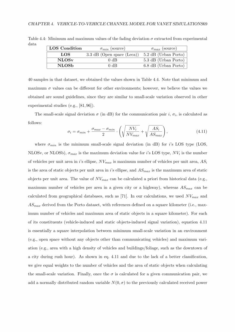
CHAPTER 4. VEHICLE-TO-VEHICLE CHANNELMODEL FOR VANET SIMULATIONS69
Table 4.4: Minimum and maximum values of the fading deviation σ extracted from experimentaldata
LOS Condition σmin (source) σmax (source)
LOS 3.3 dB (Open space (Leca)) 5.2 dB (Urban Porto)
NLOSv 0 dB 5.3 dB (Urban Porto)
NLOSb 0 dB 6.8 dB (Urban Porto)
40 samples in that dataset, we obtained the values shown in Table 4.4. Note that minimum and
maximum σ values can be different for other environments; however, we believe the values we
obtained are sound guidelines, since they are similar to small-scale variation observed in other
experimental studies (e.g., [81, 96]).
The small-scale signal deviation σ (in dB) for the communication pair i, σi, is calculated as
follows:
σi = σmin +σmax − σmin
2·(√
NViNVmax
+
√ASiASmax
), (4.11)
where σmin is the minimum small-scale signal deviation (in dB) for i’s LOS type (LOS,
NLOSv, or NLOSb), σmax is the maximum deviation value for i’s LOS type, NVi is the number
of vehicles per unit area in i’s ellipse, NVmax is maximum number of vehicles per unit area, ASi
is the area of static objects per unit area in i’s ellipse, and ASmax is the maximum area of static
objects per unit area. The value of NVmax can be calculated a priori from historical data (e.g.,
maximum number of vehicles per area in a given city or a highway), whereas ASmax can be
calculated from geographical databases, such as [71]. In our calculations, we used NVmax and
ASmax derived from the Porto dataset, with references defined on a square kilometer (i.e., max-
imum number of vehicles and maximum area of static objects in a square kilometer). For each
of its constituents (vehicle-induced and static objects-induced signal variation), equation 4.11
is essentially a square interpolation between minimum small-scale variation in an environment
(e.g., open space without any objects other than communicating vehicles) and maximum vari-
ation (e.g., area with a high density of vehicles and buildings/foliage, such as the downtown of
a city during rush hour). As shown in eq. 4.11 and due to the lack of a better classification,
we give equal weights to the number of vehicles and the area of static objects when calculating
the small-scale variation. Finally, once the σ is calculated for a given communication pair, we
add a normally distributed random variable N(0, σ) to the previously calculated received power
CHAPTER 4. VEHICLE-TO-VEHICLE CHANNELMODEL FOR VANET SIMULATIONS70
(eq. 4.6):
PrTOTi = 10 log10(Pri) +N(0, σi). (4.12)
4.4.7 Assumptions
Since we are designing a channel model with a specific application in mind – V2V communication
using IEEE 802.11p (DSRC) radios [23] or similar technology – the model relies on several
IEEE 802.11p protocol characteristics in order to simplify the implementation of our model.
Additionally, here we list other assumptions and simplifications we made when designing our
model.
1. IEEE 802.11p has been designed to cope with severe channel conditions [13]. The channel
bandwidth (10 MHz), symbol length (8 µs), guard time (1.6 µs), and Adjacent Channel
Rejection (ACR) have all been designed so that the multipath fading/Doppler spread and
Inter-Symbol Interference (ISI) do not affect the communication even in the harshest chan-
nel conditions [68]. In combination with Orthogonal Frequency-Division Multiplexing, it
is envisioned to enable flat and ISI-free channels. For this reason, in our model we assume
that the channel coherence bandwidth is sufficiently high so as not to cause frequency
selective fading on OFDM subcarriers. Experimental studies by Acosta-Marum and In-
gram in [39] and by Paier et al. in [51] confirm this assumption. However, a recent study
by Fernandez et al. in [97] point out that the proposed IEEE 802.11p physical (PHY)
layer (due to suboptimal equalization in particular) can suffer high packet error rates in
highly-faded V2V environments. In case the PHY layer of IEEE 802.11p is unable to cope
with the channel variations (thus resulting in the packet errors), the results generated by
the model above would represent the upper bound of the performance in terms of packet
delivery rate.
2. We limit the calculation of diffracted and reflected rays for NLOSb links to single-interaction
(single-bounce) rays. It was recently shown in [91] and [92] that single-interaction re-
flections and diffractions are most often the dominating propagation mechanisms in the
absence of LOS on urban intersections. However, even though communicating vehicles in
parallel streets with contiguous buildings between the streets or vehicles several streets
apart most often do not have strong single-interaction reflected or diffracted rays, they
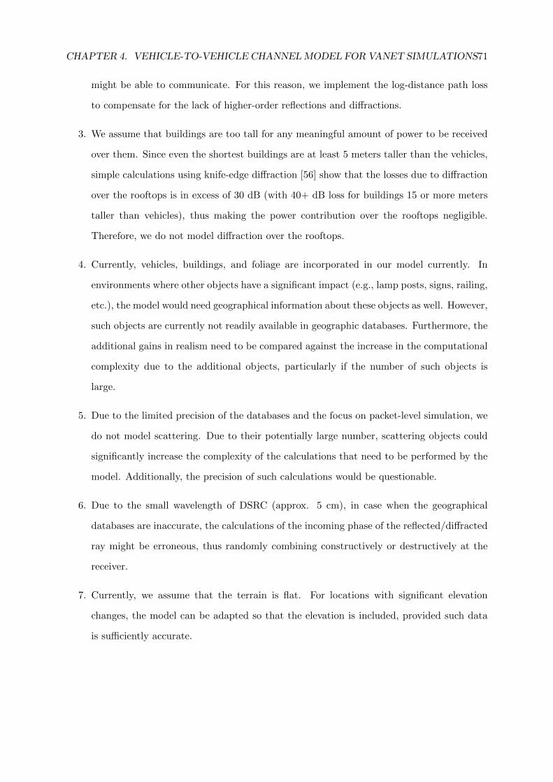
CHAPTER 4. VEHICLE-TO-VEHICLE CHANNELMODEL FOR VANET SIMULATIONS71
might be able to communicate. For this reason, we implement the log-distance path loss
to compensate for the lack of higher-order reflections and diffractions.
3. We assume that buildings are too tall for any meaningful amount of power to be received
over them. Since even the shortest buildings are at least 5 meters taller than the vehicles,
simple calculations using knife-edge diffraction [56] show that the losses due to diffraction
over the rooftops is in excess of 30 dB (with 40+ dB loss for buildings 15 or more meters
taller than vehicles), thus making the power contribution over the rooftops negligible.
Therefore, we do not model diffraction over the rooftops.
4. Currently, vehicles, buildings, and foliage are incorporated in our model currently. In
environments where other objects have a significant impact (e.g., lamp posts, signs, railing,
etc.), the model would need geographical information about these objects as well. However,
such objects are currently not readily available in geographic databases. Furthermore, the
additional gains in realism need to be compared against the increase in the computational
complexity due to the additional objects, particularly if the number of such objects is
large.
5. Due to the limited precision of the databases and the focus on packet-level simulation, we
do not model scattering. Due to their potentially large number, scattering objects could
significantly increase the complexity of the calculations that need to be performed by the
model. Additionally, the precision of such calculations would be questionable.
6. Due to the small wavelength of DSRC (approx. 5 cm), in case when the geographical
databases are inaccurate, the calculations of the incoming phase of the reflected/diffracted
ray might be erroneous, thus randomly combining constructively or destructively at the
receiver.
7. Currently, we assume that the terrain is flat. For locations with significant elevation
changes, the model can be adapted so that the elevation is included, provided such data
is sufficiently accurate.
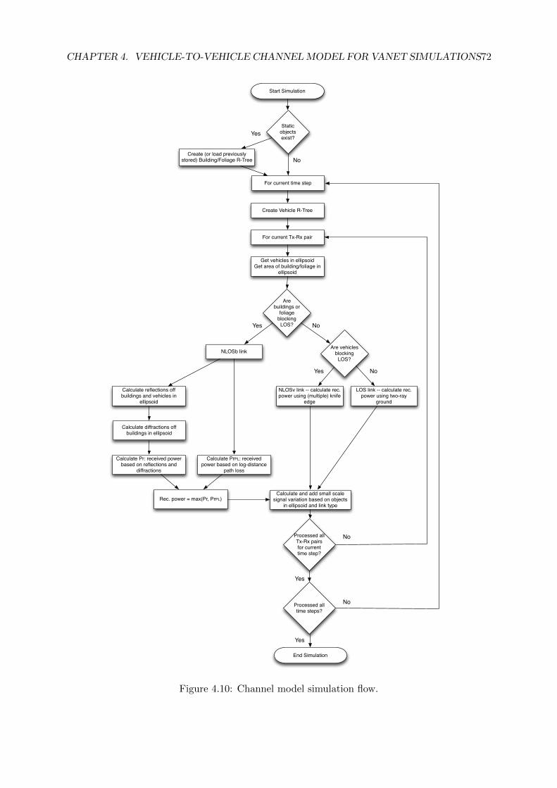
CHAPTER 4. VEHICLE-TO-VEHICLE CHANNELMODEL FOR VANET SIMULATIONS72
For current Tx-Rx pair
NLOSb link
LOS link -- calculate rec. power using two-ray
ground
NLOSv link -- calculate rec. power using (multiple) knife
edge
Create (or load previously stored) Building/Foliage R-Tree
Create Vehicle R-Tree
For current time step
Get vehicles in ellipsoidGet area of building/foliage in
ellipsoid
Yes
No
Yes No
Calculate reflections off buildings and vehicles in
ellipsoid
Calculate and add small scale signal variation based on objects
in ellipsoid and link type
Calculate PrPL: received power based on log-distance
path loss
Rec. power = max(Pr, PrPL)
Calculate diffractions off buildings in ellipsoid
Calculate Pr: received power based on reflections and
diffractions
Static objects exist?
Are buildings or
foliage blocking LOS?
Are vehicles blocking LOS?
Yes No
Processed all Tx-Rx pairs for current time step?
No
Yes
Processed all time steps?
No
Yes
Start Simulation
End Simulation
Figure 4.10: Channel model simulation flow.
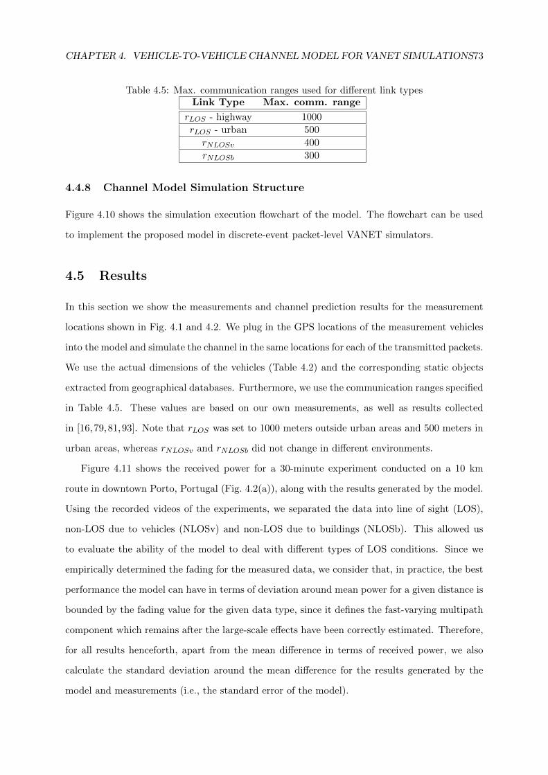
CHAPTER 4. VEHICLE-TO-VEHICLE CHANNELMODEL FOR VANET SIMULATIONS73
Table 4.5: Max. communication ranges used for different link typesLink Type Max. comm. range
rLOS - highway 1000
rLOS - urban 500
rNLOSv 400
rNLOSb 300
4.4.8 Channel Model Simulation Structure
Figure 4.10 shows the simulation execution flowchart of the model. The flowchart can be used
to implement the proposed model in discrete-event packet-level VANET simulators.
4.5 Results
In this section we show the measurements and channel prediction results for the measurement
locations shown in Fig. 4.1 and 4.2. We plug in the GPS locations of the measurement vehicles
into the model and simulate the channel in the same locations for each of the transmitted packets.
We use the actual dimensions of the vehicles (Table 4.2) and the corresponding static objects
extracted from geographical databases. Furthermore, we use the communication ranges specified
in Table 4.5. These values are based on our own measurements, as well as results collected
in [16,79,81,93]. Note that rLOS was set to 1000 meters outside urban areas and 500 meters in
urban areas, whereas rNLOSv and rNLOSb did not change in different environments.
Figure 4.11 shows the received power for a 30-minute experiment conducted on a 10 km
route in downtown Porto, Portugal (Fig. 4.2(a)), along with the results generated by the model.
Using the recorded videos of the experiments, we separated the data into line of sight (LOS),
non-LOS due to vehicles (NLOSv) and non-LOS due to buildings (NLOSb). This allowed us
to evaluate the ability of the model to deal with different types of LOS conditions. Since we
empirically determined the fading for the measured data, we consider that, in practice, the best
performance the model can have in terms of deviation around mean power for a given distance is
bounded by the fading value for the given data type, since it defines the fast-varying multipath
component which remains after the large-scale effects have been correctly estimated. Therefore,
for all results henceforth, apart from the mean difference in terms of received power, we also
calculate the standard deviation around the mean difference for the results generated by the
model and measurements (i.e., the standard error of the model).
CHAPTER 4. VEHICLE-TO-VEHICLE CHANNELMODEL FOR VANET SIMULATIONS74
Figure 4.11: Received power for a single 30-minute experiment in downtown Porto, Portugal,along with the received power predicted by the model. Number of data points: 16500.
4.5.1 LOS Links
Figure 4.12 shows the results for the LOS data in different environments. The model fits the
experimental data quite well in all environments, with the mean difference between model and
measurements within 0.6 dB for each of the environments. Similarly, the standard error for
all LOS datasets (shown in a text box in each of the subfigures of Fig. 4.12) is within 0.5 dB
of the small-scale fading for that dataset (noted in the caption of each subfigure). Regard-
ing the open space LOS results, we attribute the higher fading of the Open space Pittsburgh
dataset (Fig. 4.12(c)) compared to the Open space Porto dataset (Fig. 4.12(b)) to the guard
rails and metal fence (visible in Fig. 4.2(f)), which did not exist in the Open space Porto loca-
tion (Fig. 4.2(b)). The daytime suburban (5th Ave.) measurements (Fig. 4.12(e)) and urban
measurements in downtown Porto (Fig. 4.12(f)) have a significantly richer reflection/diffraction
environments due to the nearby vehicles in case of the former and both vehicles and buildings
in case of the latter. This results in the increase of both the fading (σ) and the standard error.
It is important to note that the mean and standard deviation of the difference in received power
between the model and experiments is performed on a per-packet basis; for each collected mea-
surement datapoint, we calculate the mean and standard deviation using the per-packet received
power difference between the model and experiments. Furthermore, we use the same value of
relative permittivity (εr=1.003) in all environments to calculate the reflection coefficient for the
ground reflection (i.e., we do not fit the value to a given dataset).
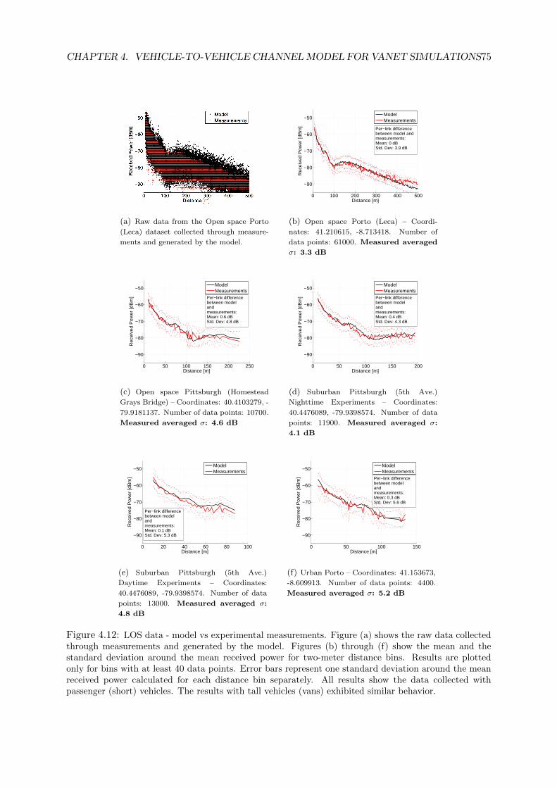
CHAPTER 4. VEHICLE-TO-VEHICLE CHANNELMODEL FOR VANET SIMULATIONS75
(a) Raw data from the Open space Porto
(Leca) dataset collected through measure-
ments and generated by the model.
0 100 200 300 400 500
−90
−80
−70
−60
−50
Distance [m]
Rec
eive
d P
ower
[dB
m]
ModelMeasurements
Per−link difference between model andmeasurements:Mean: 0 dBStd. Dev: 3.9 dB
(b) Open space Porto (Leca) – Coordi-
nates: 41.210615, -8.713418. Number of
data points: 61000. Measured averaged
σ: 3.3 dB
0 50 100 150 200 250
−90
−80
−70
−60
−50
Distance [m]
Rec
eive
d P
ower
[dB
m]
ModelMeasurements
Per−link differencebetween modelandmeasurements:Mean: 0.6 dBStd. Dev: 4.8 dB
(c) Open space Pittsburgh (Homestead
Grays Bridge) – Coordinates: 40.4103279, -
79.9181137. Number of data points: 10700.
Measured averaged σ: 4.6 dB
0 50 100 150 200
−90
−80
−70
−60
−50
Distance [m]
Rec
eive
d P
ower
[dB
m]
ModelMeasurements
Per−link differencebetween modelandmeasurements:Mean: 0.4 dBStd. Dev: 4.3 dB
(d) Suburban Pittsburgh (5th Ave.)
Nighttime Experiments – Coordinates:
40.4476089, -79.9398574. Number of data
points: 11900. Measured averaged σ:
4.1 dB
0 20 40 60 80 100
−90
−80
−70
−60
−50
Distance [m]
Rec
eive
d P
ower
[dB
m]
ModelMeasurements
Per−link differencebetween modelandmeasurements:Mean: 0.1 dBStd. Dev: 5.3 dB
(e) Suburban Pittsburgh (5th Ave.)
Daytime Experiments – Coordinates:
40.4476089, -79.9398574. Number of data
points: 13000. Measured averaged σ:
4.8 dB
0 50 100 150
−90
−80
−70
−60
−50
Distance [m]
Rec
eive
d P
ower
[dB
m]
ModelMeasurements
Per−link differencebetween modelandmeasurements:Mean: 0.3 dBStd. Dev: 5.6 dB
(f) Urban Porto – Coordinates: 41.153673,
-8.609913. Number of data points: 4400.
Measured averaged σ: 5.2 dB
Figure 4.12: LOS data - model vs experimental measurements. Figure (a) shows the raw data collectedthrough measurements and generated by the model. Figures (b) through (f) show the mean and thestandard deviation around the mean received power for two-meter distance bins. Results are plottedonly for bins with at least 40 data points. Error bars represent one standard deviation around the meanreceived power calculated for each distance bin separately. All results show the data collected withpassenger (short) vehicles. The results with tall vehicles (vans) exhibited similar behavior.
CHAPTER 4. VEHICLE-TO-VEHICLE CHANNELMODEL FOR VANET SIMULATIONS76
4.5.2 NLOSv Links
Figure 4.13 shows the results for the NLOSv data in different environments and with both pas-
senger (short) and tall vehicles. The model fits the experimental data well in all environments,
with the mean difference between model and measurements within 1.3 dB in each of the envi-
ronments. Again, the standard error for NLOSv datasets (shown in a text box in each of the
subfigures of Fig. 4.13) is within 0.9 dB of the small-scale fading of that dataset (noted in the
caption of each subfigure). It is interesting to see that NLOSv results for tall vehicles (vans)
experience both lower fading and lower standard error. This is due to the advantageous position
of the antennas on top of the vans, which are shadowed less frequently than the antennas on the
shorter vehicles. This results in a more stable channel with less fading.
4.5.3 NLOSb Links
Figure 4.14(a) shows the Porto Outlet location with the overlaid reflecting and diffracting rays
as generated by the model. Once the vehicles are not in LOS, the predominant propagation
mechanisms become single-interaction reflections and diffractions. Figure 4.14(b) shows distinct
transitions of the received power as the vehicles transition from LOS to NLOSb. The model is
able to capture the steep drop in the received power once the LOS is obstructed by building. At
the same time, the log-distance path loss, because it is unable to capture the transition between
LOS and NLOSb, underestimates the received power in LOS conditions and overestimates it in
NLOSb conditions. This result points out the importance of location-specific channel modeling:
the transitions between different LOS conditions at exact times when they occur can only be
accounted for by taking into account the objects in the location. On the other hand, models
relying on the common parameters of a large environment (such as the overall path-loss exponent
in the case of log-distance path loss) are unable to model such transitions, which results in
“averaging” of the received power between different LOS conditions. Therefore, for such models
to be useful for calculation of per-link channel characteristics, at minimum the different LOS
conditions need to be identified and modeled separately.
Furthermore, a good match between experiments and model shows that transmission through
the building does not play an important role. This confirms previous measurement studies that
made similar observations: Anderson in [86] performed experiments at 1.8 GHz and modeled the
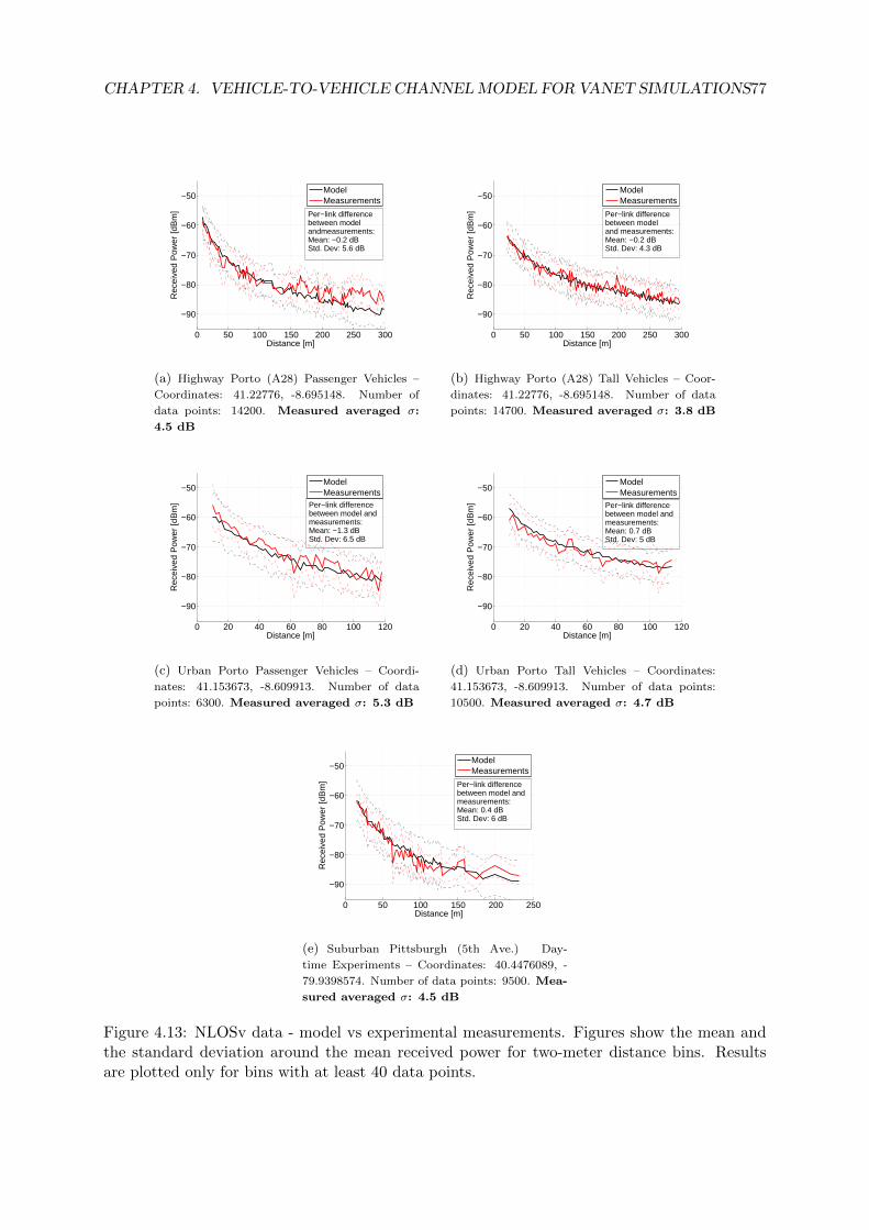
CHAPTER 4. VEHICLE-TO-VEHICLE CHANNELMODEL FOR VANET SIMULATIONS77
0 50 100 150 200 250 300
−90
−80
−70
−60
−50
Distance [m]
Rec
eive
d P
ower
[dB
m]
ModelMeasurements
Per−link differencebetween modelandmeasurements:Mean: −0.2 dBStd. Dev: 5.6 dB
(a) Highway Porto (A28) Passenger Vehicles –
Coordinates: 41.22776, -8.695148. Number of
data points: 14200. Measured averaged σ:
4.5 dB
0 50 100 150 200 250 300
−90
−80
−70
−60
−50
Distance [m]
Rec
eive
d P
ower
[dB
m]
ModelMeasurements
Per−link differencebetween modeland measurements:Mean: −0.2 dBStd. Dev: 4.3 dB
(b) Highway Porto (A28) Tall Vehicles – Coor-
dinates: 41.22776, -8.695148. Number of data
points: 14700. Measured averaged σ: 3.8 dB
0 20 40 60 80 100 120
−90
−80
−70
−60
−50
Distance [m]
Rec
eive
d P
ower
[dB
m]
ModelMeasurements
Per−link difference between model and measurements:Mean: −1.3 dBStd. Dev: 6.5 dB
(c) Urban Porto Passenger Vehicles – Coordi-
nates: 41.153673, -8.609913. Number of data
points: 6300. Measured averaged σ: 5.3 dB
0 20 40 60 80 100 120
−90
−80
−70
−60
−50
Distance [m]
Rec
eive
d P
ower
[dB
m]
ModelMeasurements
Per−link difference between model andmeasurements:Mean: 0.7 dBStd. Dev: 5 dB
(d) Urban Porto Tall Vehicles – Coordinates:
41.153673, -8.609913. Number of data points:
10500. Measured averaged σ: 4.7 dB
0 50 100 150 200 250
−90
−80
−70
−60
−50
Distance [m]
Rec
eive
d P
ower
[dB
m]
ModelMeasurements
Per−link difference between model andmeasurements:Mean: 0.4 dBStd. Dev: 6 dB
(e) Suburban Pittsburgh (5th Ave.) Day-
time Experiments – Coordinates: 40.4476089, -
79.9398574. Number of data points: 9500. Mea-
sured averaged σ: 4.5 dB
Figure 4.13: NLOSv data - model vs experimental measurements. Figures show the mean andthe standard deviation around the mean received power for two-meter distance bins. Resultsare plotted only for bins with at least 40 data points.
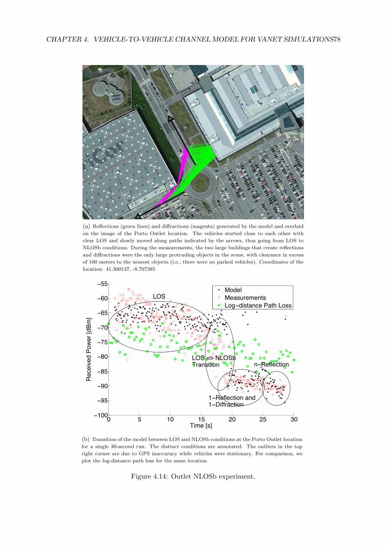
CHAPTER 4. VEHICLE-TO-VEHICLE CHANNELMODEL FOR VANET SIMULATIONS78
5.2425 5.243 5.2435 5.244 5.2445 5.245 5.2455 5.246 5.2465 5.247 5.24754.572
4.5721
4.5721
4.5722
4.5723
4.5723
4.5724x 10⁶
Wednesday, October 24, 12
(a) Reflections (green lines) and diffractions (magenta) generated by the model and overlaid
on the image of the Porto Outlet location. The vehicles started close to each other with
clear LOS and slowly moved along paths indicated by the arrows, thus going from LOS to
NLOSb conditions. During the measurements, the two large buildings that create reflections
and diffractions were the only large protruding objects in the scene, with clearance in excess
of 100 meters to the nearest objects (i.e., there were no parked vehicles). Coordinates of the
location: 41.300137, -8.707385
0 5 10 15 20 25 30−100
−95
−90
−85
−80
−75
−70
−65
−60
−55
Time [s]
Rec
eive
d Po
wer
[dBm
]
ModelMeasurementsLog−distance Path Loss
n−Reflection
1−Reflection and1−Diffraction
LOS => NLOSbTransition
LOS
(b) Transition of the model between LOS and NLOSb conditions at the Porto Outlet location
for a single 30-second run. The distinct conditions are annotated. The outliers in the top
right corner are due to GPS inaccuracy while vehicles were stationary. For comparison, we
plot the log-distance path loss for the same location.
Figure 4.14: Outlet NLOSb experiment.
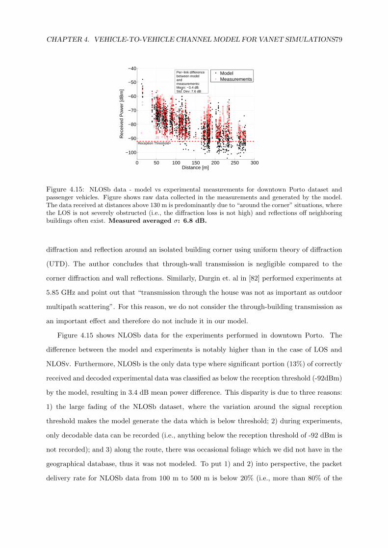
CHAPTER 4. VEHICLE-TO-VEHICLE CHANNELMODEL FOR VANET SIMULATIONS79
0 50 100 150 200 250 300
−100
−90
−80
−70
−60
−50
−40
Distance [m]
Rec
eive
d P
ower
[dB
m]
ModelMeasurements
Per−link difference between modelandmeasurements:Mean: −3.4 dBStd. Dev: 7.6 dB
Reception Threshold
Figure 4.15: NLOSb data - model vs experimental measurements for downtown Porto dataset andpassenger vehicles. Figure shows raw data collected in the measurements and generated by the model.The data received at distances above 130 m is predominantly due to “around the corner” situations, wherethe LOS is not severely obstructed (i.e., the diffraction loss is not high) and reflections off neighboringbuildings often exist. Measured averaged σ: 6.8 dB.
diffraction and reflection around an isolated building corner using uniform theory of diffraction
(UTD). The author concludes that through-wall transmission is negligible compared to the
corner diffraction and wall reflections. Similarly, Durgin et. al in [82] performed experiments at
5.85 GHz and point out that “transmission through the house was not as important as outdoor
multipath scattering”. For this reason, we do not consider the through-building transmission as
an important effect and therefore do not include it in our model.
Figure 4.15 shows NLOSb data for the experiments performed in downtown Porto. The
difference between the model and experiments is notably higher than in the case of LOS and
NLOSv. Furthermore, NLOSb is the only data type where significant portion (13%) of correctly
received and decoded experimental data was classified as below the reception threshold (-92dBm)
by the model, resulting in 3.4 dB mean power difference. This disparity is due to three reasons:
1) the large fading of the NLOSb dataset, where the variation around the signal reception
threshold makes the model generate the data which is below threshold; 2) during experiments,
only decodable data can be recorded (i.e., anything below the reception threshold of -92 dBm is
not recorded); and 3) along the route, there was occasional foliage which we did not have in the
geographical database, thus it was not modeled. To put 1) and 2) into perspective, the packet
delivery rate for NLOSb data from 100 m to 500 m is below 20% (i.e., more than 80% of the
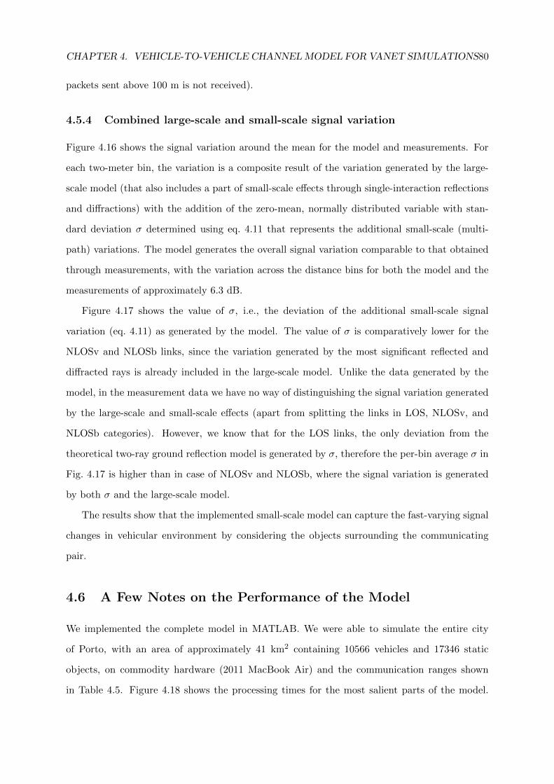
CHAPTER 4. VEHICLE-TO-VEHICLE CHANNELMODEL FOR VANET SIMULATIONS80
packets sent above 100 m is not received).
4.5.4 Combined large-scale and small-scale signal variation
Figure 4.16 shows the signal variation around the mean for the model and measurements. For
each two-meter bin, the variation is a composite result of the variation generated by the large-
scale model (that also includes a part of small-scale effects through single-interaction reflections
and diffractions) with the addition of the zero-mean, normally distributed variable with stan-
dard deviation σ determined using eq. 4.11 that represents the additional small-scale (multi-
path) variations. The model generates the overall signal variation comparable to that obtained
through measurements, with the variation across the distance bins for both the model and the
measurements of approximately 6.3 dB.
Figure 4.17 shows the value of σ, i.e., the deviation of the additional small-scale signal
variation (eq. 4.11) as generated by the model. The value of σ is comparatively lower for the
NLOSv and NLOSb links, since the variation generated by the most significant reflected and
diffracted rays is already included in the large-scale model. Unlike the data generated by the
model, in the measurement data we have no way of distinguishing the signal variation generated
by the large-scale and small-scale effects (apart from splitting the links in LOS, NLOSv, and
NLOSb categories). However, we know that for the LOS links, the only deviation from the
theoretical two-ray ground reflection model is generated by σ, therefore the per-bin average σ in
Fig. 4.17 is higher than in case of NLOSv and NLOSb, where the signal variation is generated
by both σ and the large-scale model.
The results show that the implemented small-scale model can capture the fast-varying signal
changes in vehicular environment by considering the objects surrounding the communicating
pair.
4.6 A Few Notes on the Performance of the Model
We implemented the complete model in MATLAB. We were able to simulate the entire city
of Porto, with an area of approximately 41 km2 containing 10566 vehicles and 17346 static
objects, on commodity hardware (2011 MacBook Air) and the communication ranges shown
in Table 4.5. Figure 4.18 shows the processing times for the most salient parts of the model.
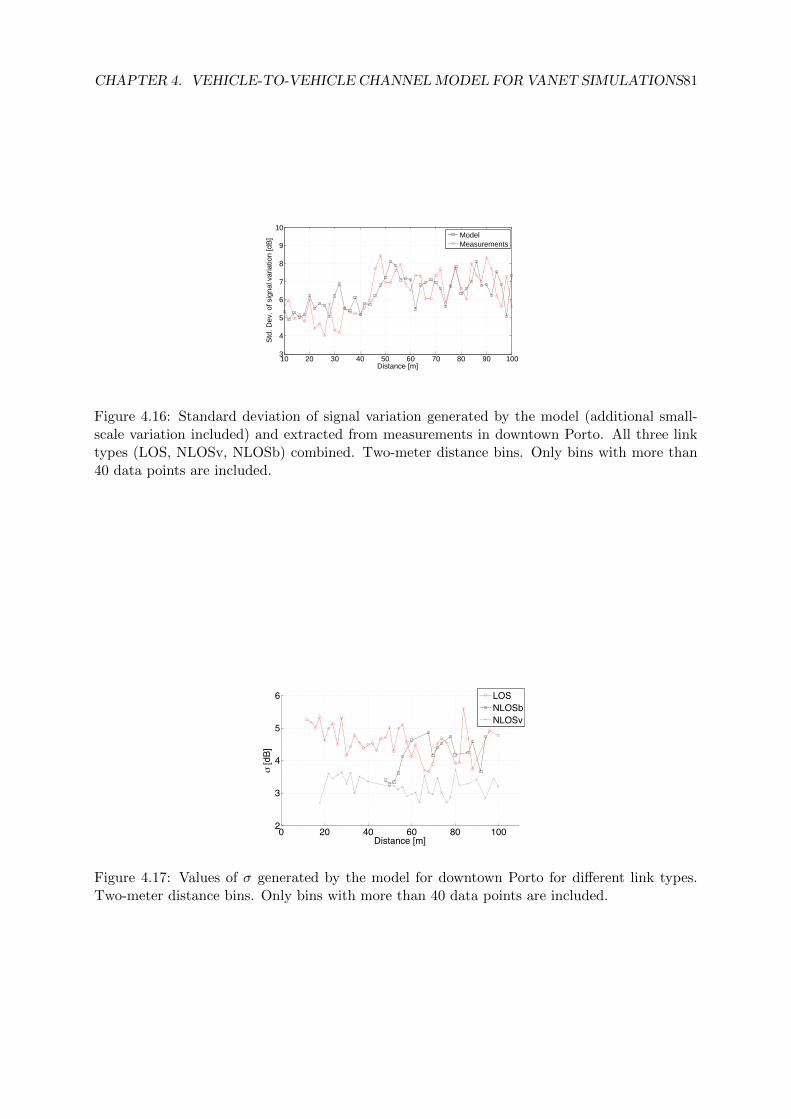
CHAPTER 4. VEHICLE-TO-VEHICLE CHANNELMODEL FOR VANET SIMULATIONS81
10 20 30 40 50 60 70 80 90 1003
4
5
6
7
8
9
10
Distance [m]
Std
. Dev
. of s
igna
l var
iatio
n [d
B]
ModelMeasurements
Figure 4.16: Standard deviation of signal variation generated by the model (additional small-scale variation included) and extracted from measurements in downtown Porto. All three linktypes (LOS, NLOSv, NLOSb) combined. Two-meter distance bins. Only bins with more than40 data points are included.
0 20 40 60 80 1002
3
4
5
6
Distance [m]
σ [d
B]
LOSNLOSbNLOSv
Figure 4.17: Values of σ generated by the model for downtown Porto for different link types.Two-meter distance bins. Only bins with more than 40 data points are included.
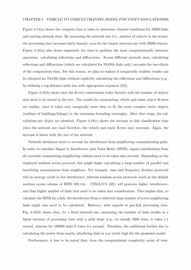
CHAPTER 4. VEHICLE-TO-VEHICLE CHANNELMODEL FOR VANET SIMULATIONS82
Figure 4.18(a) shows the complete time it takes to determine channel conditions for 10000 links
and varying network sizes. By increasing the network size (i.e., number of objects in the scene),
the processing time increases fairly linearly, even for the largest network size with 28000 objects.
Figure 4.18(a) also shows separately the time to perform the most computationally intensive
operation: calculating reflections and diffractions. Across different network sizes, calculating
reflections and diffractions (which are calculated for NLOSb links only) accounts for two-thirds
of the computation time. For this reason, we plan to explore if comparably realistic results can
be obtained for NLOSb links without explicitly calculating the reflections and diffractions (e.g.,
by utilizing a log-distance path loss with appropriate exponent [24]).
Figure 4.18(b) shows that the R-tree construction scales linearly with the number of objects
that need to be stored in the tree. The results for constructing vehicle and static object R-trees
are similar, since it takes only marginally more time to fit the more complex static objects
(outlines of buildings/foliage) in the minimum bounding rectangles. After that stage, the cal-
culations per object are identical. Figure 4.18(c) shows the increase in link classification time
when the network size (and therefore, the vehicle and static R-tree size) increases. Again, the
increase is linear with the size of the network.
Network simulators need to account for interference from neighboring communicating pairs.
In order to calculate Signal to Interference plus Noise Ratio (SINR), signal contributions from
all currently transmitting neighboring vehicles need to be taken into account. Depending on the
employed medium access protocol, this might imply calculating a large number of parallel and
interfering transmissions from neighbors. For example, time and frequency division protocols
will on average result in low interference, whereas random access protocols (such as the default
medium access scheme of IEEE 802.11p – CSMA/CA [68]) will generate higher interference,
and thus higher number of links that need to be taken into consideration. This implies that, to
calculate the SINR for a link, the interference from a relatively large number of active neighboring
links might also need to be calculated. However, with regards to per-link processing time,
Fig. 4.18(d) shows that, for a fixed network size, increasing the number of links results in a
linear increase of processing time with a mild slope (e.g., to classify 5000 links, it takes 1.1
second, whereas for 100000 links it takes 3.1 second). Therefore, the additional burden due to
calculating the power from nearby interfering links is not overly high for the proposed model.
Furthermore, it has to be noted that, from the computational complexity point of view,
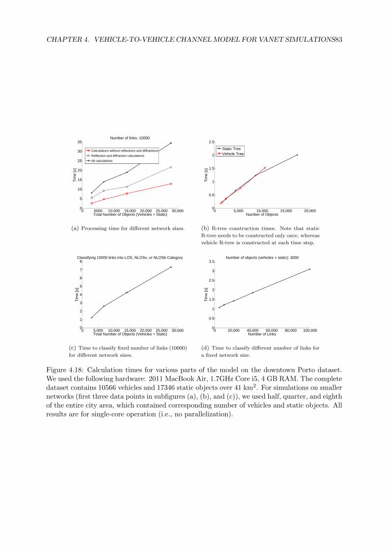
CHAPTER 4. VEHICLE-TO-VEHICLE CHANNELMODEL FOR VANET SIMULATIONS83
0 5000 10,000 15,000 20,000 25,000 30,0000
5
10
15
20
25
30
35
Tim
e [s
]
Total Number of Objects (Vehicles + Static)
Number of links: 10000
Calculations without reflections and diffractions
Reflection and diffraction calculations
All calculations
(a) Processing time for different network sizes.
0 5,000 10,000 15,000 20,0000
0.5
1
1.5
2
2.5
Number of Objects
Tim
e [s
]
Static TreeVehicle Tree
(b) R-tree construction times. Note that static
R-tree needs to be constructed only once, whereas
vehicle R-tree is constructed at each time step.
0 5,000 10,000 15,000 20,000 25,000 30,0000
1
2
3
4
5
6
7
8
Total Number of Objects (Vehicles + Static)
Tim
e [s
]
Classifying 10000 links into LOS, NLOSv, or NLOSb Category
(c) Time to classify fixed number of links (10000)
for different network sizes.
0 20,000 40,000 60,000 80,000 100,0000
0.5
1
1.5
2
2.5
3
3.5
Number of Links
Tim
e [s
]
Number of objects (vehicles + static): 3000
(d) Time to classify different number of links for
a fixed network size.
Figure 4.18: Calculation times for various parts of the model on the downtown Porto dataset.We used the following hardware: 2011 MacBook Air, 1.7GHz Core i5, 4 GB RAM. The completedataset contains 10566 vehicles and 17346 static objects over 41 km2. For simulations on smallernetworks (first three data points in subfigures (a), (b), and (c)), we used half, quarter, and eighthof the entire city area, which contained corresponding number of vehicles and static objects. Allresults are for single-core operation (i.e., no parallelization).
CHAPTER 4. VEHICLE-TO-VEHICLE CHANNELMODEL FOR VANET SIMULATIONS84
selecting the correct communication range if quite important. Increasing the range results in
quadratic increase in the number of objects neighboring a given communication pair. By design,
in the extreme case, if the communication range is equal to the size of the simulated area,
the number of neighboring objects (and therefore calculations) is quadratic with the number
of communicating pairs. Therefore, the communication range for each of the LOS types needs
to be carefully chosen so that it is minimized while accounting for potentially communicating
pairs.
With regards to the scalability of the model, the trends shown in Fig. 4.18 are far more
important than the actual processing times. The result show linear behavior even for large
networks comprising tens of thousands of objects and communicating pairs. We also point
out that the operations required by the model (R-tree construction and classification of links
through object querying and intersection tests) are inherently parallelizable. Since the model
relies on geometric manipulations of the objects that impact the channel, analogies can be made
to computer graphics domain, where parallel rendering techniques are utilized to perform oc-
clusion/visibility and intersection testing [98,99]. Parallelization techniques can be employed in
both the object querying and intersection testing, as well as the R-tree construction. Since there
is no dependency between different communication pairs (links), parallelizing the computations
across different links is straightforward. Furthermore, recent advances in parallel R-tree con-
struction, querying, and intersection testing (e.g., see Luo et. al in [100]) indicate that significant
speed increase can be obtained by using multicore graphics processing units.
4.7 Related Work
Several recent studies tackled efficient and realistic simulation of vehicle-to-vehicle channels
in different VANET environments. Karedal et al. in [79] and Mangel et al. in [101] designed
channel models focused on street intersections, where buildings create non-LOS (NLOSb) con-
ditions. Both studies selected representative urban intersections and performed measurements
which were then used to design channel models and calibrate the path loss and fading param-
eters. Karedal et al. in [50] designed a V2V channel model based on measurements performed
in highway and suburban environment at the 5.2 GHz frequency band. The model distributes
the vehicles and static objects randomly and analyzes four distinct signal components: LOS,
CHAPTER 4. VEHICLE-TO-VEHICLE CHANNELMODEL FOR VANET SIMULATIONS85
discrete components from vehicles, discrete components from static objects, and diffuse scatter-
ing. Based on the measurements, the authors propose a set of model parameters for highway
and suburban environment. While it enables modeling of different propagation characteristics
(path loss, multipath, Doppler spread, etc.), the proposed model assumes the LOS component
exists, therefore it does not specify how to determine the LOS conditions of the channel and the
transitions between LOS, NLOSv, and NLOSb. Figure 4.14 shows that modeling the transitions
between the LOS conditions is essential for obtaining realistic results, since the ensuing path
loss is the most important component in determining the received power and, consequently, the
decodability of the packet.
Sommer et al. in [102] perform measurements based on which they calibrate a computation-
ally efficient path loss model aimed at distinguishing between the LOS and NLOSb conditions.
The authors design the model based on the assumption that transmission through buildings is
the main propagation mechanism, while diffractions and reflections are not modeled. This goes
against previous experimental and modeling studies reported by Anderson in [86] and Durgin
et al. in [82], which concluded that reflections and diffractions are the dominant propagation
mechanisms in the 1.9 and 5.9 GHz frequency bands. Furthermore, the results we obtained in
isolated experiments (Fig. 4.14) show that the V2V channel obstructed by buildings for DSRC
systems in the 5.9 GHz band is well represented by accounting for diffractions and reflections
only, thus indicating that the transmission through buildings plays a minor role.
In terms of channel modeling on a city-wide scale, studies reported by Giordano et al. in [94],
Martinez et al. in [103], and Cozzetti et al. in [104] focus on computationally efficient channel
modeling in grid-like urban environments, where streets are assumed to be straight and inter-
secting at a right angle. While such assumptions hold for certain urban areas, in others they
might be overly simple (e.g., in the city of Porto – Fig. 4.5).
With regards to improving the channel modeling using location-specific information, Wang
et al. in [72] utilize aerial photography to determine the density of scatterers in the simulated
area. By processing the aerial data to infer the scatterer density, the authors determine the
fading level for a given location on the road.
A number of studies were performed in various VANET environments to estimate the chan-
nel by performing measurements and fitting the measured data using well-known models (e.g.,
log-distance path loss [57]). Cheng et al. in [24] performed measurements in suburban Pitts-
CHAPTER 4. VEHICLE-TO-VEHICLE CHANNELMODEL FOR VANET SIMULATIONS86
burgh, PA, USA, in the 5.9 GHz frequency band. The authors fit the measurement data to a
dual slope piecewise log-distance path loss model (i.e., they use two path loss exponents and
two fading deviations). They also make an observation that buildings and vehicles significantly
impact the received power and that there exists a need for “a multi-state model, with different
states being applicable when a line of sight does and does not exist between the vehicles”. Sim-
ilarly, Paschalidis et al. in [95] make measurements in different environments (urban, suburban,
rural, highway) and fit the measurements data to the log-distance path loss model. Again, the
path loss exponent varies considerably (between 1.83 and 3.59) for different locations and LOS
conditions. The large range of path loss exponent reported in these studies goes to show that
a single path loss exponent can not capture the characteristics of a channel, even for a single
location/environment. Therefore, different LOS conditions (LOS, NLOSv, NLOSb) need to be
distinguished and modeled separately.
When it comes to evaluating the impact of vehicular obstructions, several experimental
studies emphasized the importance of obstructing vehicles. Sepulcre et al. in [105] and Gallagher
et al. in [106] quantified the impact of vehicular obstructions on different parameters, such as
packet reception, throughput, and communication range. Interestingly, Gonzalvez et al. in [107]
perform experiments where the impact of vehicular traffic and tall vehicles (buses) also heavily
influenced the vehicle-to-infrastructure (V2I) links, where roadside units are placed at elevated
positions (between 3 and 10 meters) next to or above the roads. Tall vehicles decreased the
effective communication range by 40%, whereas the dense traffic reduced the range by more
than 50%. Furthermore, other studies suggested that obstructing vehicles could be an important
factor in channel modeling (e.g., [14, 32,36,38]).
The studies above were aimed at measuring the channel characteristics and fitting the channel
models to the already collected measurements. However, research aimed at incorporating the
vehicles in the channel model and therefore predicting their effect has been scarce. Apart from
our previous work reported in [15], to the best of our knowledge, there have only been two studies
aimed at explicitly introducing vehicular obstruction in channel modeling. Abbas et al. in [96]
performed V2V measurements and showed that a single vehicle can incur more than 10 dB
attenuation, which is in line with the results reported in [15]. Based on the measurements, the
authors design a stochastic channel model for highway environments that incorporates vehicular
obstructions and determines the time duration of the LOS, NLOSv, and NLOSb states using
CHAPTER 4. VEHICLE-TO-VEHICLE CHANNELMODEL FOR VANET SIMULATIONS87
the measured probability distributions of each state. Wang et al. in [108] perform isolated
(“parking lot”) measurements and characterize the loss due to vehicles obstructing the LOS.
Furthermore, they model the loss due to vehicles by employing a three-ray knife-edge model,
where diffraction loss is calculated over the vehicles and on the vehicle sides using the modified
Bullington method [109]. The results show a good agreement between the isolated measurement
results and the proposed method.
4.8 Conclusions
We proposed a computationally efficient channel model that can be used in large scale packet-
level VANET simulators. Compared to the simple statistical channel models currently used in
VANET simulators, the proposed model utilizes the geographic descriptors to enable location-
specific per-link modeling of the channel. Furthermore, the time-dependent component of the
channel is accounted for: depending on the density of the vehicles in an area, the channel be-
tween two vehicles can change considerably as the surrounding vehicles create LOS obstruction,
reflections, and diffractions. Compared to the ray-tracing methods, the model is beneficial in
terms of: 1) computational complexity, since it performs only a subset of complex calculations
required for full ray-tracing models; and 2) reduced requirements for geographical information –
the only information required are outlines and type of buildings and foliage, and locations and
dimensions of vehicles – these are freely available through geographical databases and mobility
traces.
Furthermore, with limited (and often imperfect) geographical description of the simulated
area, at a certain level of simulation detail, there is a point of diminishing returns, where a
marginal improvement in the realism requires a large computational effort. For this reason, we
used VANET-specific information (e.g., number of surrounding objects, dimensions of vehicles,
different attenuation levels due to different object types, etc.) to limit the complexity of the
model. To enable a more efficient channel modeling, we separated the links into three cate-
gories: 1) line of sight (LOS); 2) non-LOS due to vehicles (NLOSv); and 3) non-LOS due to
buildings/foliage (NLOSb). The results regarding LOS and NLOSv conditions shown in figs. 4.12
and 4.13 indicate that, in order to correctly model LOS and NLOSv scenarios, it is sufficient
to consider the main type of propagation mechanism for respective link type (two-ray for LOS
CHAPTER 4. VEHICLE-TO-VEHICLE CHANNELMODEL FOR VANET SIMULATIONS88
and vehicles-as-obstacles for NLOSv), with added fading proportional to the number of vehicles
and area of the static objects (buildings, foliage) in the communicating pair’s ellipse (as defined
in Fig. 4.7). This allows for an efficient implementation in the simulation environments, as the
only operations required are LOS classification and determining the number and area of objects
in the communication pair’s ellipse (both of which can be performed efficiently using bounding
volume hierarchies). On the other hand, for NLOSb cases, it is beneficial to consider reflections
and diffractions, as they enable for a better estimation of the received power, particularly when
vehicles are communicating “around the corner” (i.e., where vehicles are on two sides of a corner
of a single building, as shown in Figs. 4.14(a) and 4.14(b)). In such scenarios, not accounting
for reflected and diffracted rays would imply that the level of obstruction (i.e., the “depth” of
the building corner with respect to LOS path) is not important. However, due to reflections and
diffractions accounting for two thirds of the computation time, as part of our future work, we
will look for alternative techniques for channel estimation for NLOSb links.
We implemented the model and showed that it can be used to simulate networks containing
thousands of communicating vehicles across different environments (highway, suburban, urban).
The model is able to simulate city-wide areas containing buildings and foliage. The results
showed that the model behaves linearly with the increase of both the network size (i.e., number
of objects in the simulation) and the number of communicating pairs.

Chapter 5
TVR – Tall Vehicle Relaying
In Chapters 2 and 3, we have shown that line of sight (LOS) conditions have a direct influence on
V2V link quality. LOS is influenced by both mobile objects (vehicles) and static objects (build-
ings, foliage) located between and around the communicating nodes. We have shown experimen-
tally that vehicles can obstruct the LOS communication up to 50% of the time; furthermore, a
single obstructing vehicle can reduce the power at the receiver by more than 20 dB. Similarly,
buildings obstructing the LOS severely impede communication, with under 20% of packets suc-
cessfully delivered when the distance between the communicating pair is above 100 m. Based on
both experimental measurements (Ch. 2) and simulations performed using the proposed chan-
nel model (Ch. 3 and 4), in this chapter we show that the elevated position of the antennas on
tall vehicles significantly improves communication performance. Tall vehicles can increase the
effective communication range, with an improvement of up to 50% in certain scenarios [69,110].
Using these findings, we propose a new V2V relaying scheme called Tall Vehicle Relaying (TVR)
that takes advantage of the better channel characteristics provided by tall vehicles. TVR distin-
guishes between tall and short vehicles and, where appropriate, chooses tall vehicles as next hop
relays. We investigate TVR’s system-level performance through a combination of small-scale
experiments and large-scale simulations and show that it outperforms existing techniques.
5.1 Motivation
The relatively low height of the antennas located on the vehicles makes V2V communication
susceptible to line of sight (LOS) obstruction by non-communicating vehicles. The probability
89
CHAPTER 5. TVR – TALL VEHICLE RELAYING 90
of having LOS communication decreases with distance, with less than a 50% chance of LOS
near the maximum V2V communication range [15]. Furthermore, the Dedicated Short-Range
Communications (DSRC) [23] frequency band reserved for VANET communication is in the
5.9 GHz band. As noted by Parsons in [57], in this frequency band the “propagation paths must
have line of sight between the transmitting and receiving antennas, otherwise losses are extremely
high”. This has been empirically shown to be the case for V2V links in [16], where a single
large truck attenuated the received power between two passenger cars by 27 dB. Consequently,
obstructing vehicles cause a reduction of the effective communication range of up to 60% and
Packet Delivery Ratio (PDR) of up to 30%, depending on the environment.
Motivated by these findings, we explore how the adverse effects of vehicular obstructions
can be ameliorated by opting for the taller vehicles as next hop relays. We distinguish between
tall vehicles, such as commercial and public transportation vehicles (vans, buses, trucks, etc.)
and short vehicles (passenger cars). We base this distinction on the analysis performed in [15],
which showed that the dimensions of the most popular passenger cars differ significantly from
the dimensions of commercial freight and public transportation vehicles. Specifically, it was
observed that the latter are, on average, more than 1.5 meters taller than personal vehicles. By
separating the vehicles in this manner, we showed in [69,110] that the antennas mounted on top
of tall vehicles experience a significantly better communication channel, which is not as affected
by obstruction from other vehicles as is the case for short vehicles (i.e., the probability of having
LOS increases).
We perform small-scale experiments and large-scale simulations that provide insights into the
end-to-end benefits of tall vehicle relaying. Based on the benefits we observed while performing
experiments, we introduce the Tall Vehicle Relaying (TVR) technique, a paradigm shift from
the farthest relay technique, which selects the farthest tall vehicle in the direction of message
destination. We compare the performance of TVR with two techniques: i) Farthest Neighbor,
which selects the farthest neighbor with which communication is possible; and ii) and Most New
Neighbors, which selects the vehicle with the largest number of new neighbors in the direction of
message dissemination. The results show that TVR matches these techniques in lower vehicle
density scenarios and outperforms them in high density scenarios in terms of the number of hops
required to reach a destination and end-to-end delay.
The main contributions of this work can be summarized as follows:
CHAPTER 5. TVR – TALL VEHICLE RELAYING 91
• Leveraging previous results based on aerial photography and a validated channel model, we
quantify the benefits of using tall vehicles as next hops in terms of: 1) LOS communication;
2) received signal power; and 3) effective communication range;
• We perform real-world experiments to determine the benefits of using tall vehicles as relays;
the results show that selecting tall vehicles is beneficial in terms of higher received power,
smaller number of hops to reach the destination (thus decreasing end-to-end delay), and
increased per-hop communication range;
• We introduce the Tall Vehicle Relay (TVR) technique, which matches existing techniques
in low vehicle density scenarios and outperforms them in high density scenarios in terms
of the number of hops needed to reach the destination, delay, and medium contention.
The rest of the chapter is organized as follows. Model-based analysis of selecting tall vehi-
cles as relays is presented in Section 5.2. The experimental setup and results are described in
Section 5.3. Section 5.4 describes the TVR technique and the results of the large-scale simula-
tions, whereas Section 5.5 describes related work. Finally, Section 5.6 provides conclusions and
discusses possible future work.
5.2 Model-Based Analysis of the Benefits of Tall Vehicles as
Relays
In this section we analyze the effect of vehicle height on the probability of line of sight and on
the received signal strength. The discussion on Packet Delivery Ratio (PDR) is deferred to the
next section in order to facilitate comparison with the experimentally obtained data.
5.2.1 Setup
To assess the effect of tall vehicles on communication performance, apart from experimental
evaluation, we also designed a large-scale simulative study. For the study to be credible, we
require the following: 1) accurate information on vehicle positions and dimensions; and 2) a
realistic channel model.
For accurate vehicle positioning, we leverage a dataset of real vehicle positions obtained from
aerial photography of the A28 highway located near Porto, Portugal. The 404 vehicle dataset is
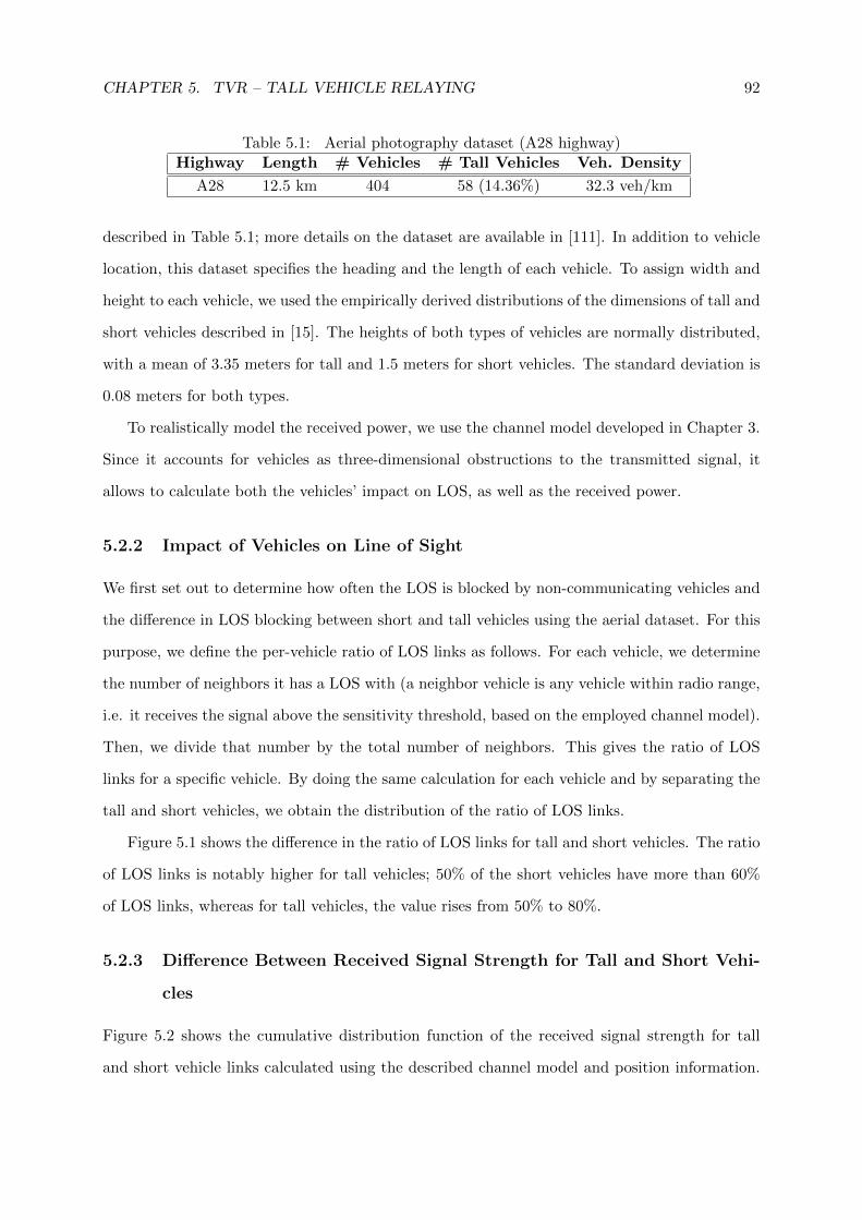
CHAPTER 5. TVR – TALL VEHICLE RELAYING 92
Table 5.1: Aerial photography dataset (A28 highway)Highway Length # Vehicles # Tall Vehicles Veh. Density
A28 12.5 km 404 58 (14.36%) 32.3 veh/km
described in Table 5.1; more details on the dataset are available in [111]. In addition to vehicle
location, this dataset specifies the heading and the length of each vehicle. To assign width and
height to each vehicle, we used the empirically derived distributions of the dimensions of tall and
short vehicles described in [15]. The heights of both types of vehicles are normally distributed,
with a mean of 3.35 meters for tall and 1.5 meters for short vehicles. The standard deviation is
0.08 meters for both types.
To realistically model the received power, we use the channel model developed in Chapter 3.
Since it accounts for vehicles as three-dimensional obstructions to the transmitted signal, it
allows to calculate both the vehicles’ impact on LOS, as well as the received power.
5.2.2 Impact of Vehicles on Line of Sight
We first set out to determine how often the LOS is blocked by non-communicating vehicles and
the difference in LOS blocking between short and tall vehicles using the aerial dataset. For this
purpose, we define the per-vehicle ratio of LOS links as follows. For each vehicle, we determine
the number of neighbors it has a LOS with (a neighbor vehicle is any vehicle within radio range,
i.e. it receives the signal above the sensitivity threshold, based on the employed channel model).
Then, we divide that number by the total number of neighbors. This gives the ratio of LOS
links for a specific vehicle. By doing the same calculation for each vehicle and by separating the
tall and short vehicles, we obtain the distribution of the ratio of LOS links.
Figure 5.1 shows the difference in the ratio of LOS links for tall and short vehicles. The ratio
of LOS links is notably higher for tall vehicles; 50% of the short vehicles have more than 60%
of LOS links, whereas for tall vehicles, the value rises from 50% to 80%.
5.2.3 Difference Between Received Signal Strength for Tall and Short Vehi-
cles
Figure 5.2 shows the cumulative distribution function of the received signal strength for tall
and short vehicle links calculated using the described channel model and position information.
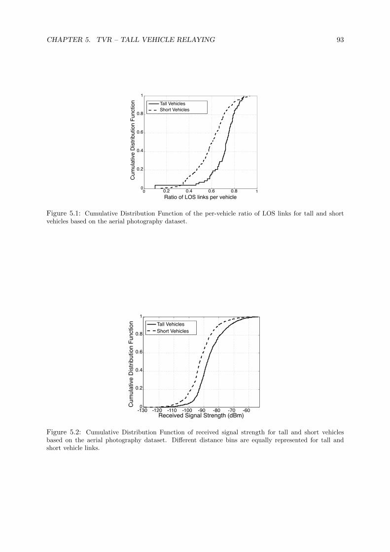
CHAPTER 5. TVR – TALL VEHICLE RELAYING 93
0 0.2 0.4 0.6 0.8 10
0.2
0.4
0.6
0.8
1
Ratio of LOS links per vehicle
Cum
ulat
ive D
istrib
utio
n Fu
nctio
n
Tall VehiclesShort Vehicles
Figure 5.1: Cumulative Distribution Function of the per-vehicle ratio of LOS links for tall and shortvehicles based on the aerial photography dataset.
-130 -120 -110 -100 -90 -80 70 -600
0.2
0.4
0.6
0.8
1
Received Signal Strength (dBm)
Cum
ulat
ive
Dis
tribu
tion
Func
tion
Tall VehiclesShort Vehicles
-
Figure 5.2: Cumulative Distribution Function of received signal strength for tall and short vehiclesbased on the aerial photography dataset. Different distance bins are equally represented for tall andshort vehicle links.
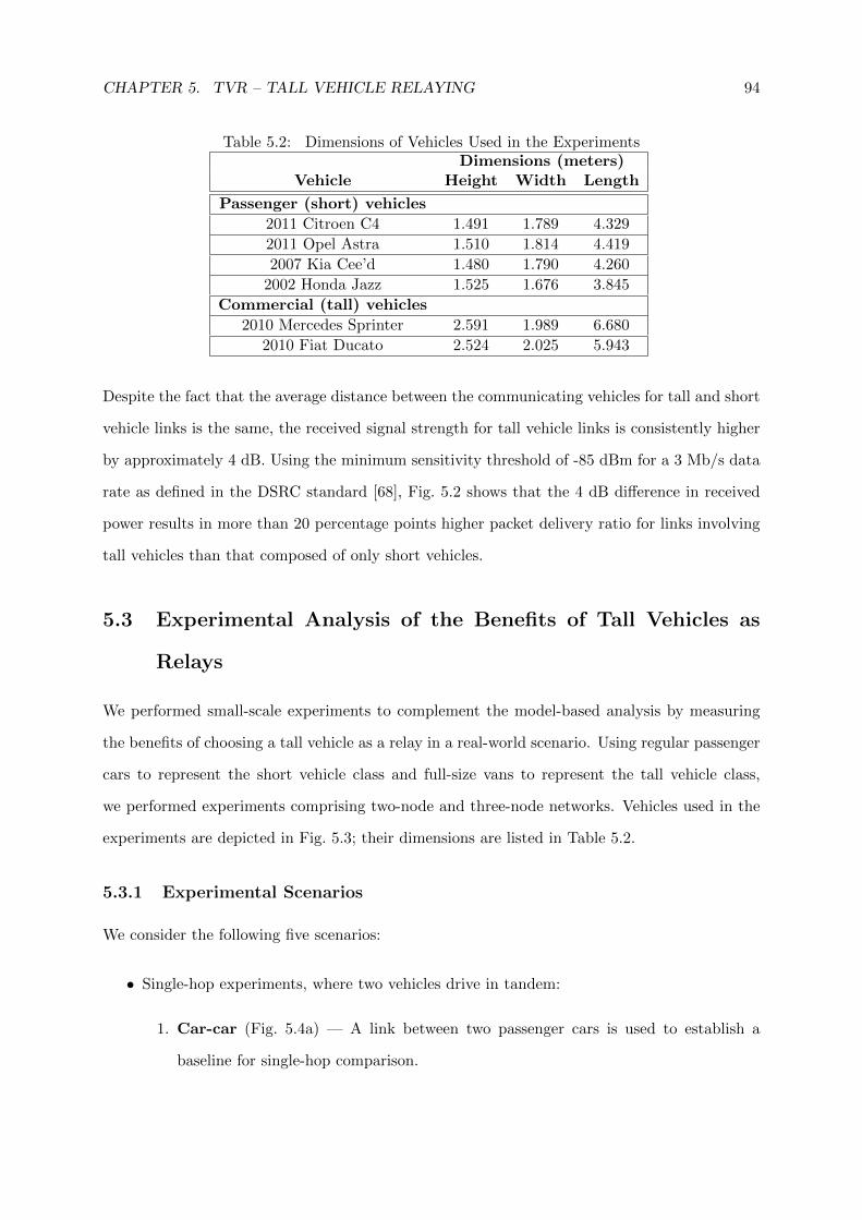
CHAPTER 5. TVR – TALL VEHICLE RELAYING 94
Table 5.2: Dimensions of Vehicles Used in the ExperimentsDimensions (meters)
Vehicle Height Width Length
Passenger (short) vehicles
2011 Citroen C4 1.491 1.789 4.329
2011 Opel Astra 1.510 1.814 4.419
2007 Kia Cee’d 1.480 1.790 4.260
2002 Honda Jazz 1.525 1.676 3.845
Commercial (tall) vehicles
2010 Mercedes Sprinter 2.591 1.989 6.680
2010 Fiat Ducato 2.524 2.025 5.943
Despite the fact that the average distance between the communicating vehicles for tall and short
vehicle links is the same, the received signal strength for tall vehicle links is consistently higher
by approximately 4 dB. Using the minimum sensitivity threshold of -85 dBm for a 3 Mb/s data
rate as defined in the DSRC standard [68], Fig. 5.2 shows that the 4 dB difference in received
power results in more than 20 percentage points higher packet delivery ratio for links involving
tall vehicles than that composed of only short vehicles.
5.3 Experimental Analysis of the Benefits of Tall Vehicles as
Relays
We performed small-scale experiments to complement the model-based analysis by measuring
the benefits of choosing a tall vehicle as a relay in a real-world scenario. Using regular passenger
cars to represent the short vehicle class and full-size vans to represent the tall vehicle class,
we performed experiments comprising two-node and three-node networks. Vehicles used in the
experiments are depicted in Fig. 5.3; their dimensions are listed in Table 5.2.
5.3.1 Experimental Scenarios
We consider the following five scenarios:
• Single-hop experiments, where two vehicles drive in tandem:
1. Car-car (Fig. 5.4a) — A link between two passenger cars is used to establish a
baseline for single-hop comparison.
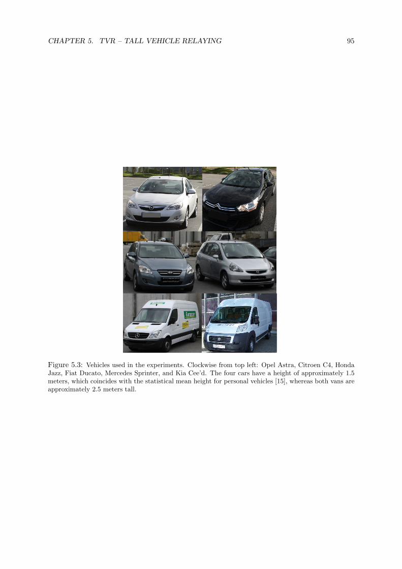
CHAPTER 5. TVR – TALL VEHICLE RELAYING 95
4$
Figure 5.3: Vehicles used in the experiments. Clockwise from top left: Opel Astra, Citroen C4, HondaJazz, Fiat Ducato, Mercedes Sprinter, and Kia Cee’d. The four cars have a height of approximately 1.5meters, which coincides with the statistical mean height for personal vehicles [15], whereas both vans areapproximately 2.5 meters tall.
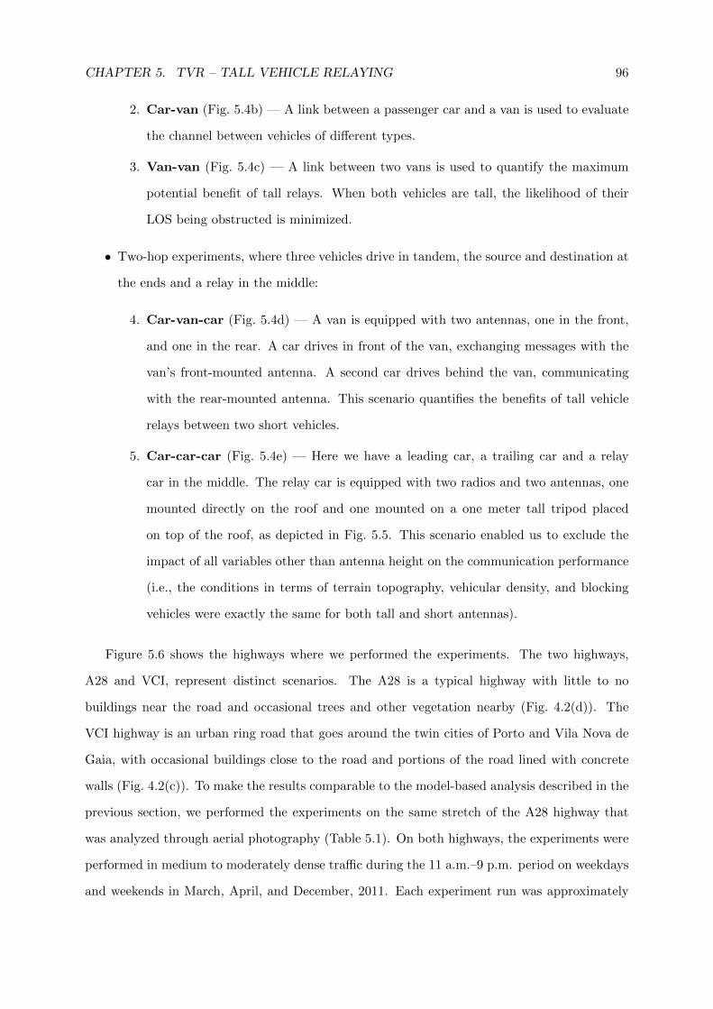
CHAPTER 5. TVR – TALL VEHICLE RELAYING 96
2. Car-van (Fig. 5.4b) — A link between a passenger car and a van is used to evaluate
the channel between vehicles of different types.
3. Van-van (Fig. 5.4c) — A link between two vans is used to quantify the maximum
potential benefit of tall relays. When both vehicles are tall, the likelihood of their
LOS being obstructed is minimized.
• Two-hop experiments, where three vehicles drive in tandem, the source and destination at
the ends and a relay in the middle:
4. Car-van-car (Fig. 5.4d) — A van is equipped with two antennas, one in the front,
and one in the rear. A car drives in front of the van, exchanging messages with the
van’s front-mounted antenna. A second car drives behind the van, communicating
with the rear-mounted antenna. This scenario quantifies the benefits of tall vehicle
relays between two short vehicles.
5. Car-car-car (Fig. 5.4e) — Here we have a leading car, a trailing car and a relay
car in the middle. The relay car is equipped with two radios and two antennas, one
mounted directly on the roof and one mounted on a one meter tall tripod placed
on top of the roof, as depicted in Fig. 5.5. This scenario enabled us to exclude the
impact of all variables other than antenna height on the communication performance
(i.e., the conditions in terms of terrain topography, vehicular density, and blocking
vehicles were exactly the same for both tall and short antennas).
Figure 5.6 shows the highways where we performed the experiments. The two highways,
A28 and VCI, represent distinct scenarios. The A28 is a typical highway with little to no
buildings near the road and occasional trees and other vegetation nearby (Fig. 4.2(d)). The
VCI highway is an urban ring road that goes around the twin cities of Porto and Vila Nova de
Gaia, with occasional buildings close to the road and portions of the road lined with concrete
walls (Fig. 4.2(c)). To make the results comparable to the model-based analysis described in the
previous section, we performed the experiments on the same stretch of the A28 highway that
was analyzed through aerial photography (Table 5.1). On both highways, the experiments were
performed in medium to moderately dense traffic during the 11 a.m.–9 p.m. period on weekdays
and weekends in March, April, and December, 2011. Each experiment run was approximately
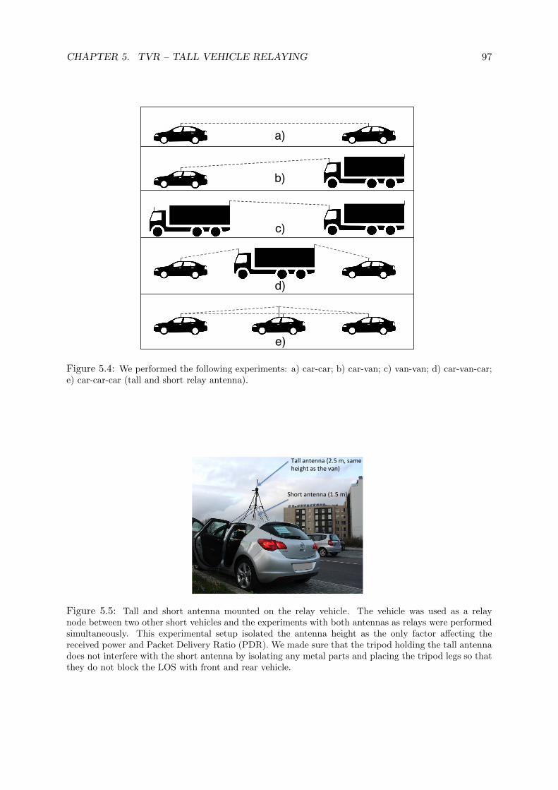
CHAPTER 5. TVR – TALL VEHICLE RELAYING 97
a)
b)
c)
d)
e)
Figure 5.4: We performed the following experiments: a) car-car; b) car-van; c) van-van; d) car-van-car;e) car-car-car (tall and short relay antenna).
Tall$antenna$(2.5$m,$same$$height$as$the$van)$
Short$antenna$(1.5$m)$
Monday, March 19, 12
Figure 5.5: Tall and short antenna mounted on the relay vehicle. The vehicle was used as a relaynode between two other short vehicles and the experiments with both antennas as relays were performedsimultaneously. This experimental setup isolated the antenna height as the only factor affecting thereceived power and Packet Delivery Ratio (PDR). We made sure that the tripod holding the tall antennadoes not interfere with the short antenna by isolating any metal parts and placing the tripod legs so thatthey do not block the LOS with front and rear vehicle.
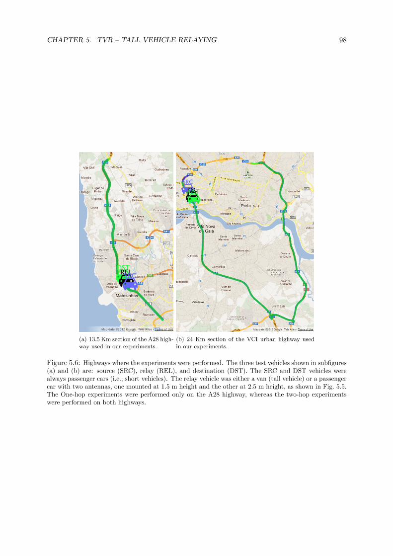
CHAPTER 5. TVR – TALL VEHICLE RELAYING 98
(a) 13.5 Km section of the A28 high-way used in our experiments.
(b) 24 Km section of the VCI urban highway usedin our experiments.
Figure 5.6: Highways where the experiments were performed. The three test vehicles shown in subfigures(a) and (b) are: source (SRC), relay (REL), and destination (DST). The SRC and DST vehicles werealways passenger cars (i.e., short vehicles). The relay vehicle was either a van (tall vehicle) or a passengercar with two antennas, one mounted at 1.5 m height and the other at 2.5 m height, as shown in Fig. 5.5.The One-hop experiments were performed only on the A28 highway, whereas the two-hop experimentswere performed on both highways.
CHAPTER 5. TVR – TALL VEHICLE RELAYING 99
one hour long, with the vehicles traversing the A28 highway south to north and vice versa and
making an incomplete loop on the VCI highway as shown in Fig. 5.6. Speeds ranged from 40
to 120 km/h, in accordance with traffic conditions. The single-hop experiments were performed
on A28, whereas the two-hop experiments were performed on both A28 and VCI.
5.3.2 Hardware Setup
Vehicles were equipped with NEC LinkBird-MXs V3, a development platform for vehicular
communications, described in section 2.2.1. Each node was configured to send periodic position
beacons that were then used to record Received Signal Strength Indicator (RSSI) and Packet
Delivery Ratio (PDR) information during the experiments (PDR is defined as the the ratio
between the number of received messages and the number of sent messages). The position
information was obtained from an external GPS receiver connected to each LinkBird. The
system parameters are shown in Table 2.1.
On the passenger cars, the antenna was positioned at the center of the roof, which has been
empirically shown to be the overall optimal position [31]. On the vans, we used two antennas:
one at the front of the roof, and another at the back (shown in Fig. 5.4). This prevents the
van itself from significantly deteriorating the channel characteristics by blocking the LOS path
between its own antenna and the antenna of the vehicle it is communicating with.
We distinguish two types of links: 1) line of sight (LOS); and 2) non-LOS due to vehicles
(NLOSv)1. To help us distinguish between LOS and NLOSv conditions, we recorded videos of
the experiments from the vehicle following in the rear in case of single-hop, and from both the
leading and trailing vehicles in case of two-hop experiments (two videos were required in two-
hop experiments to determine LOS conditions for each link). We then synchronized the videos
to the experimental data using a custom web-based visualization suite [112] and classified each
part of the experiment as LOS or NLOSv with a one second resolution. We classified the
conditions as NLOSv when one or more vehicles, short or tall, were present between the two
communicating vehicles. Given that the experiments were performed on highways, the number
of static obstructions such as buildings was negligible and thus not considered.
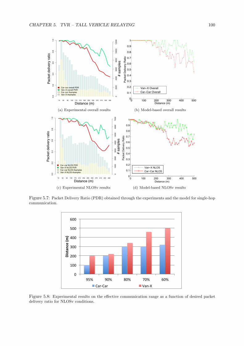
CHAPTER 5. TVR – TALL VEHICLE RELAYING 100
10 50 90 130 170 210 250 290 330 370 410 450 490
020
0040
0060
0080
0010
000
1200
0
0.0
0.2
0.4
0.6
0.8
1.0
Distance (m)
Pack
et d
elive
ry ra
tio
# sa
mpl
es
Car−car overall PDRVan−X overall PDRCar−car #samplesVan−X #samples
(a) Experimental overall results
0 100 200 300 400 5000
0.1
0.2
0.3
0.4
0.5
0.6
0.7
0.8
0.9
1
Distance (m)
Pack
et D
eliv
ery
Rat
io
Van−X Overall Car−Car Overall
(b) Model-based overall results
10 50 90 130 170 210 250 290 330 370 410 450 490
010
0020
0030
0040
0050
0060
0070
00
0.0
0.2
0.4
0.6
0.8
1.0
Distance (m)
Pack
et d
elive
ry ra
tio
# sa
mpl
es
Car−car NLOS PDRVan−X NLOS PDRCar−car NLOS #samplesVan−X NLOS #samples
(c) Experimental NLOSv results
! "!! #!! $!! %!! &!!!
!'"
!'#
!'$
!'%
!'&
!'(
!')
!'*
!'+
"
,-./01234567
80293/4,3:-;3<=4>0/-?
4
4
@01AB4CDEFG0<AG0<4CDEF
(d) Model-based NLOSv results
Figure 5.7: Packet Delivery Ratio (PDR) obtained through the experiments and the model for single-hopcommunication.
0
100
200
300
400
500
600
95% 90% 80% 70% 60%
Distan
ce (m
)
Car-‐Car Van-‐X
Figure 5.8: Experimental results on the effective communication range as a function of desired packetdelivery ratio for NLOSv conditions.
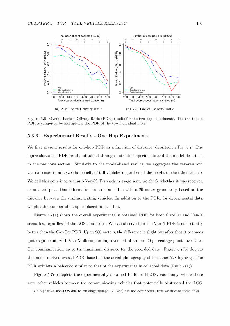
CHAPTER 5. TVR – TALL VEHICLE RELAYING 101
200 300 400 500 600 700 800 900
0.0
0.2
0.4
0.6
0.8
1.0
7 32 29 36 29 18 11 12
Total source−destination distance (m)
Pac
ket D
eliv
ery
Rat
io (
PD
R)
Number of sent packets (x1000)
VanCar short antennaCar tall antenna
(a) A28 Packet Delivery Ratio
200 300 400 500 600 700 800 900
0.0
0.2
0.4
0.6
0.8
1.0
29 32 27 14 15 16 4 4
Total source−destination distance (m)
Pac
ket D
eliv
ery
Rat
io (
PD
R)
Number of sent packets (x1000)
VanCar short antennaCar tall antenna
(b) VCI Packet Delivery Ratio
Figure 5.9: Overall Packet Delivery Ratio (PDR) results for the two-hop experiments. The end-to-endPDR is computed by multiplying the PDR of the two individual links.
5.3.3 Experimental Results - One Hop Experiments
We first present results for one-hop PDR as a function of distance, depicted in Fig. 5.7. The
figure shows the PDR results obtained through both the experiments and the model described
in the previous section. Similarly to the model-based results, we aggregate the van-van and
van-car cases to analyze the benefit of tall vehicles regardless of the height of the other vehicle.
We call this combined scenario Van-X. For each message sent, we check whether it was received
or not and place that information in a distance bin with a 20 meter granularity based on the
distance between the communicating vehicles. In addition to the PDR, for experimental data
we plot the number of samples placed in each bin.
Figure 5.7(a) shows the overall experimentally obtained PDR for both Car-Car and Van-X
scenarios, regardless of the LOS conditions. We can observe that the Van-X PDR is consistently
better than the Car-Car PDR. Up to 280 meters, the difference is slight but after that it becomes
quite significant, with Van-X offering an improvement of around 20 percentage points over Car-
Car communication up to the maximum distance for the recorded data. Figure 5.7(b) depicts
the model-derived overall PDR, based on the aerial photography of the same A28 highway. The
PDR exhibits a behavior similar to that of the experimentally collected data (Fig 5.7(a)).
Figure 5.7(c) depicts the experimentally obtained PDR for NLOSv cases only, where there
were other vehicles between the communicating vehicles that potentially obstructed the LOS.
1On highways, non-LOS due to buildings/foliage (NLOSb) did not occur often, thus we discard these links.
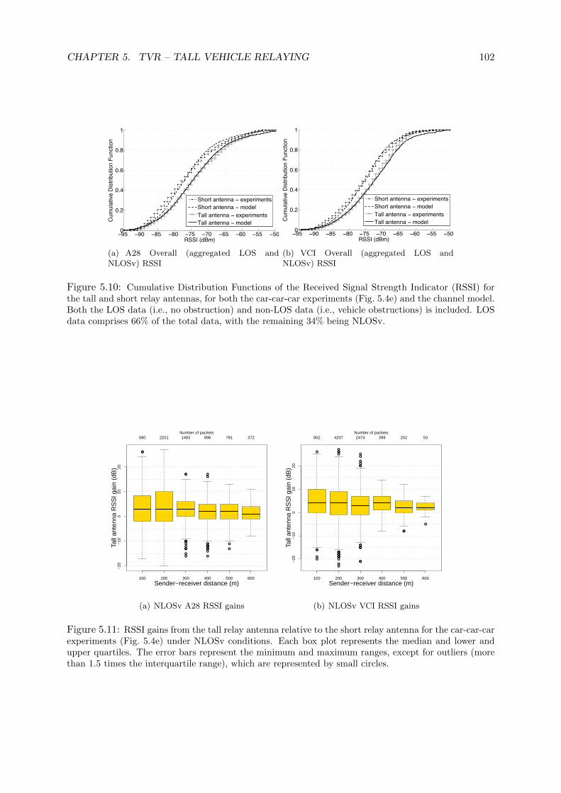
CHAPTER 5. TVR – TALL VEHICLE RELAYING 102
−95 −90 −85 −80 −75 −70 −65 −60 −55 −500
0.2
0.4
0.6
0.8
1
RSSI (dBm)
Cum
ulat
ive
Dis
tribu
tion
Func
tion
A28 RSSI
Short antenna − experimentsShort antenna − modelTall antenna − experimentsTall antenna − model
(a) A28 Overall (aggregated LOS andNLOSv) RSSI
−95 −90 −85 −80 −75 −70 −65 −60 −55 −500
0.2
0.4
0.6
0.8
1
RSSI (dBm)
Cum
ulat
ive
Dis
tribu
tion
Func
tion
VCI RSSI
Short antenna − experimentsShort antenna − modelTall antenna − experimentsTall antenna − model
(b) VCI Overall (aggregated LOS andNLOSv) RSSI
Figure 5.10: Cumulative Distribution Functions of the Received Signal Strength Indicator (RSSI) forthe tall and short relay antennas, for both the car-car-car experiments (Fig. 5.4e) and the channel model.Both the LOS data (i.e., no obstruction) and non-LOS data (i.e., vehicle obstructions) is included. LOSdata comprises 66% of the total data, with the remaining 34% being NLOSv.
●●
●
●●
●
●
●
●
●
●
●
●●
●
●
●●●●●●●●
●
●
●
●●
●
●
●
100 200 300 400 500 600
−20
−10
010
20
580 2251 1483 896 781 372
Sender−receiver distance (m)
Tall
ante
nna
RS
SI g
ain
(dB
)
Number of packets
(a) NLOSv A28 RSSI gains
●
●
●●
●
●
●●●
●
●
●
●
●●
●
●●
●
●
●
●●
●
●
●
●●
●
●●
●●
●
●
●●●
●
●
●●
●
100 200 300 400 500 600
−20
−10
010
20
852 4207 2474 399 252 53
Sender−receiver distance (m)
Tall
ante
nna
RS
SI g
ain
(dB
)
Number of packets
(b) NLOSv VCI RSSI gains
Figure 5.11: RSSI gains from the tall relay antenna relative to the short relay antenna for the car-car-carexperiments (Fig. 5.4e) under NLOSv conditions. Each box plot represents the median and lower andupper quartiles. The error bars represent the minimum and maximum ranges, except for outliers (morethan 1.5 times the interquartile range), which are represented by small circles.
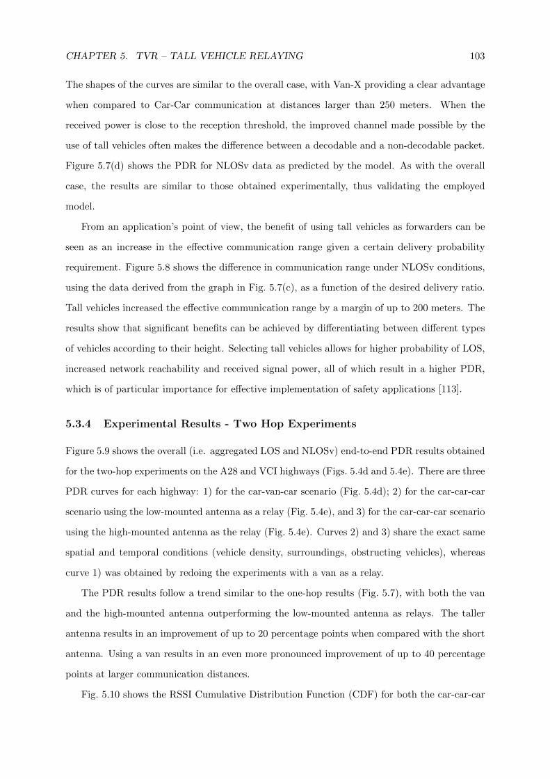
CHAPTER 5. TVR – TALL VEHICLE RELAYING 103
The shapes of the curves are similar to the overall case, with Van-X providing a clear advantage
when compared to Car-Car communication at distances larger than 250 meters. When the
received power is close to the reception threshold, the improved channel made possible by the
use of tall vehicles often makes the difference between a decodable and a non-decodable packet.
Figure 5.7(d) shows the PDR for NLOSv data as predicted by the model. As with the overall
case, the results are similar to those obtained experimentally, thus validating the employed
model.
From an application’s point of view, the benefit of using tall vehicles as forwarders can be
seen as an increase in the effective communication range given a certain delivery probability
requirement. Figure 5.8 shows the difference in communication range under NLOSv conditions,
using the data derived from the graph in Fig. 5.7(c), as a function of the desired delivery ratio.
Tall vehicles increased the effective communication range by a margin of up to 200 meters. The
results show that significant benefits can be achieved by differentiating between different types
of vehicles according to their height. Selecting tall vehicles allows for higher probability of LOS,
increased network reachability and received signal power, all of which result in a higher PDR,
which is of particular importance for effective implementation of safety applications [113].
5.3.4 Experimental Results - Two Hop Experiments
Figure 5.9 shows the overall (i.e. aggregated LOS and NLOSv) end-to-end PDR results obtained
for the two-hop experiments on the A28 and VCI highways (Figs. 5.4d and 5.4e). There are three
PDR curves for each highway: 1) for the car-van-car scenario (Fig. 5.4d); 2) for the car-car-car
scenario using the low-mounted antenna as a relay (Fig. 5.4e), and 3) for the car-car-car scenario
using the high-mounted antenna as the relay (Fig. 5.4e). Curves 2) and 3) share the exact same
spatial and temporal conditions (vehicle density, surroundings, obstructing vehicles), whereas
curve 1) was obtained by redoing the experiments with a van as a relay.
The PDR results follow a trend similar to the one-hop results (Fig. 5.7), with both the van
and the high-mounted antenna outperforming the low-mounted antenna as relays. The taller
antenna results in an improvement of up to 20 percentage points when compared with the short
antenna. Using a van results in an even more pronounced improvement of up to 40 percentage
points at larger communication distances.
Fig. 5.10 shows the RSSI Cumulative Distribution Function (CDF) for both the car-car-car
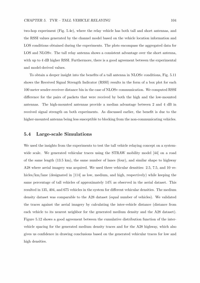
CHAPTER 5. TVR – TALL VEHICLE RELAYING 104
two-hop experiment (Fig. 5.4e), where the relay vehicle has both tall and short antennas, and
the RSSI values generated by the channel model based on the vehicle location information and
LOS conditions obtained during the experiments. The plots encompass the aggregated data for
LOS and NLOSv. The tall relay antenna shows a consistent advantage over the short antenna,
with up to 4 dB higher RSSI. Furthermore, there is a good agreement between the experimental
and model-derived values.
To obtain a deeper insight into the benefits of a tall antenna in NLOSv conditions, Fig. 5.11
shows the Received Signal Strength Indicator (RSSI) results in the form of a box plot for each
100 meter sender-receiver distance bin in the case of NLOSv communication. We computed RSSI
difference for the pairs of packets that were received by both the high and the low-mounted
antennas. The high-mounted antennas provide a median advantage between 2 and 4 dB in
received signal strength on both experiments. As discussed earlier, the benefit is due to the
higher-mounted antenna being less susceptible to blocking from the non-communicating vehicles.
5.4 Large-scale Simulations
We used the insights from the experiments to test the tall vehicle relaying concept on a system-
wide scale. We generated vehicular traces using the STRAW mobility model [44] on a road
of the same length (13.5 km), the same number of lanes (four), and similar shape to highway
A28 where aerial imagery was acquired. We used three vehicular densities: 2.5, 7.5, and 10 ve-
hicles/km/lane (designated in [114] as low, medium, and high, respectively) while keeping the
same percentage of tall vehicles of approximately 14% as observed in the aerial dataset. This
resulted in 135, 404, and 675 vehicles in the system for different vehicular densities. The medium
density dataset was comparable to the A28 dataset (equal number of vehicles). We validated
the traces against the aerial imagery by calculating the inter-vehicle distance (distance from
each vehicle to its nearest neighbor for the generated medium density and the A28 dataset).
Figure 5.12 shows a good agreement between the cumulative distribution function of the inter-
vehicle spacing for the generated medium density traces and for the A28 highway, which also
gives us confidence in drawing conclusions based on the generated vehicular traces for low and
high densities.
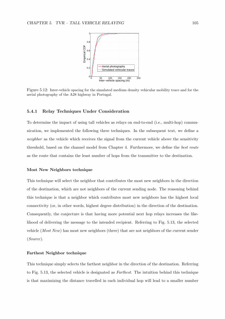
CHAPTER 5. TVR – TALL VEHICLE RELAYING 105
0 50 100 150 200 2500
0.2
0.4
0.6
0.8
1
Inter−vehicle spacing (m)E
mpi
rical
CD
F
Aerial photographySimulated vehicular traces
Figure 5.12: Inter-vehicle spacing for the simulated medium density vehicular mobility trace and for theaerial photography of the A28 highway in Portugal.
5.4.1 Relay Techniques Under Consideration
To determine the impact of using tall vehicles as relays on end-to-end (i.e., multi-hop) commu-
nication, we implemented the following three techniques. In the subsequent text, we define a
neighbor as the vehicle which receives the signal from the current vehicle above the sensitivity
threshold, based on the channel model from Chapter 4. Furthermore, we define the best route
as the route that contains the least number of hops from the transmitter to the destination.
Most New Neighbors technique
This technique will select the neighbor that contributes the most new neighbors in the direction
of the destination, which are not neighbors of the current sending node. The reasoning behind
this technique is that a neighbor which contributes most new neighbors has the highest local
connectivity (or, in other words, highest degree distribution) in the direction of the destination.
Consequently, the conjecture is that having more potential next hop relays increases the like-
lihood of delivering the message to the intended recipient. Referring to Fig. 5.13, the selected
vehicle (Most New) has most new neighbors (three) that are not neighbors of the current sender
(Source).
Farthest Neighbor technique
This technique simply selects the farthest neighbor in the direction of the destination. Referring
to Fig. 5.13, the selected vehicle is designated as Farthest. The intuition behind this technique
is that maximizing the distance travelled in each individual hop will lead to a smaller number
CHAPTER 5. TVR – TALL VEHICLE RELAYING 106
FARTHEST
MOST NEW
FARTHEST TALL
SOURCE
DESTINATION
Figure 5.13: Relay selection for the three techniques. In case of Most New Neighbors relay technique,the vehicle designated Most New Neighbors will be selected, as it has most new neighbors (three) in thedirection of the destination (designated Destination) that are not neighbors of the current sending node(designated Source). In case of Farthest Neighbor relay technique, vehicle designated Farthest Neighborwill be selected, as it is farthest from the current sending node, and in the direction of the destinationDest. In the case of TVR, the tall vehicle designated Farthest Tall will be selected. Note that a singlevehicle can be selected by multiple techniques (e.g., farthest vehicle might have most new neighbors, andit can also be a tall vehicle, which would make it the best relay for all three techniques)
of hops to reach the destination. This technique has often been used in the literature (e.g.,
see [63]).
TVR technique
Based on the benefits we observed when performing the tall vehicle experiments (see Figs. 5.7, 5.8, 5.9),
we implemented a technique that selects the farthest tall vehicle in the direction of the mes-
sage destination (Fig. 5.13), provided that dist(Tx, FarShort)−dist(Tx, FarTall) ≤ xmax, where
dist(x, y) is the Euclidean distance between points x and y, xmax is the maximum distance dif-
ference at which a tall vehicle is still a better relay, Tx is the location of the transmitter, and
FarShort and FarTall are the locations of the farthest reachable short and tall neighbors, respec-
tively. In other words, TVR selects a tall vehicle if the distance difference between the farthest
tall vehicle and the current transmitter and the farthest short vehicle and the transmitter is less
than a threshold xmax; otherwise, the farthest short node is selected.
At each hop, we define the vehicle selected by a given technique as the best relay for that
technique.
5.4.2 Calculating xmax
In order to calculate xmax, we first look at the distribution of distance difference dist(Tx, FarShort)−
dist(Tx, FarTall), as shown in Fig. 5.14, which was derived from aerial photography. The case
when a tall vehicle is the best relay (in terms of least number of end-to-end hops) is the distri-
CHAPTER 5. TVR – TALL VEHICLE RELAYING 107
bution colored red, whereas the case when a short vehicle is the best relay is colored black. To
determine when a tall vehicle is more likely to be a better relay, let us define a binary random
variable θ as being one when a tall vehicle is more likely to be a better relay, and zero otherwise:
θ =
1, when
∫ x−∞ fT (t)dt∫+∞x fS(s)ds
> 1;
0, otherwise,
(5.1)
where fT (t) and fS(s) are probability distributions of dist(Tx, FarShort) − dist(Tx, FarTall)
for best tall vehicle and best short vehicle case, respectively. In other words, we can interpret
eq. 5.1 as θ = 1 when the cumulative distribution FT (t) for a given value x is larger than the
complementary cumulative distribution of FS(s) and θ = 0 otherwise.
In order to calculate the maximum distance difference xmax at which a tall vehicle is still
a better relay, we need to solve FT (t) = 1 − FS(s). In the specific case of our collected data,
for tractability purposes we approximate the distance difference distributions of s and t with
normal distributions (normal fits shown in Fig. 5.14). In this case, xmax can be calculated by
solving
1−Q(xmax − µs
σs
)= Q
(xmax − µt
σt
), (5.2)
where µs, σs, µt, and σt are the means and variances of s and t, respectively, and Q(·) is the
Q-function, defined as Q(x) = 1√2π
∫∞x exp
(−u2
2
)du.
Figure 5.14 shows the distributions of s and t for a single transmit power (10 dBm); to
analyze the behavior of s and t with different communication ranges, we vary the transmission
power from 1 to 20 dBm. Distributions of s and t are readily available in simulators by im-
plementing an appropriate channel model (such as [15]), since the global network knowledge
(“oracle”) is available. However, obtaining these distributions is not straightforward without
global knowledge, which means that the distributions of s and t will not be available to the
routing protocols in the real world. Therefore, we set a fixed value for xmax. We used a value
of xmax calculated based on the aerial photography dataset in Table 5.1 as follows. We choose
xmax to be the average value of t across transmission powers from 1 to 20 dBm (typical transmit
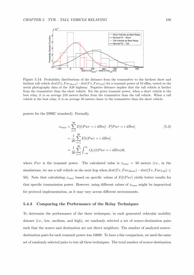
CHAPTER 5. TVR – TALL VEHICLE RELAYING 108
−100 0 100 200 300 400 500 6000
1
2
3
4
5
x 10−3
dist(Tx,FarShort) − dist(Tx,FarTall) [m]
Prob
abilit
y D
ensi
ty F
unct
ion Short Vehicle as Best Relay
Normal Fit − ShortTall Vehicle as Best RelayNormal Fit − Tall
Figure 5.14: Probability distributions of the distance from the transmitter to the farthest short andfarthest tall vehicle dist(Tx, FarShort)−dist(Tx, FarTall) for a transmit power of 10 dBm, tested on theaerial photography data of the A28 highway. Negative distance implies that the tall vehicle is fartherfrom the transmitter than the short vehicle. For the given transmit power, when a short vehicle is thebest relay, it is on average 210 meters farther from the transmitter than the tall vehicle. When a tallvehicle is the best relay, it is on average 50 meters closer to the transmitter than the short vehicle.
powers for the DSRC standard). Formally,
xmax =20∑i=1
E[t|Pwr = i dBm] · P [Pwr = i dBm] (5.3)
=1
20
20∑i=1
E[t|Pwr = i dBm]
=1
20
20∑i=1
∫ ∞−∞
tfT (t|Pwr = i dBm)dt,
where Pwr is the transmit power. The calculated value is xmax = 50 meters (i.e., in the
simulations, we use a tall vehicle as the next hop when dist(Tx, FarShort)−dist(Tx, FarTall) ≤
50). Note that calculating xmax based on specific values of E[t|Pwr] yields better results for
that specific transmission power. However, using different values of xmax might be impractical
for protocol implementation, as it may vary across different environments.
5.4.3 Comparing the Performance of the Relay Techniques
To determine the performance of the three techniques, in each generated vehicular mobility
dataset (i.e., low, medium, and high), we randomly selected a set of source-destination pairs
such that the source and destination are not direct neighbors. The number of analyzed source-
destination pairs for each transmit power was 10000. To have a fair comparison, we used the same
set of randomly selected pairs to test all three techniques. The total number of source-destination
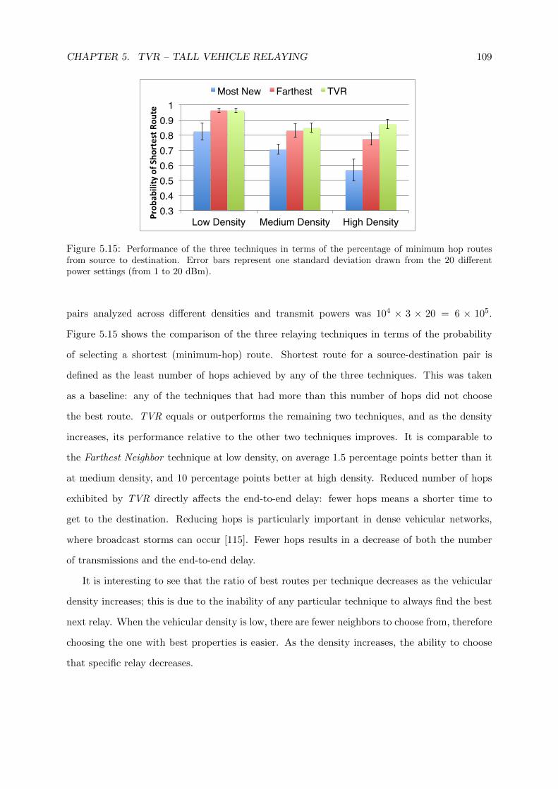
CHAPTER 5. TVR – TALL VEHICLE RELAYING 109
0.3!0.4!0.5!0.6!0.7!0.8!0.9!
1!
Low Density! Medium Density! High Density!Prob
ability of S
hortest R
oute
Most New! Farthest! TVR!
Figure 5.15: Performance of the three techniques in terms of the percentage of minimum hop routesfrom source to destination. Error bars represent one standard deviation drawn from the 20 differentpower settings (from 1 to 20 dBm).
pairs analyzed across different densities and transmit powers was 104 × 3 × 20 = 6 × 10⁵.
Figure 5.15 shows the comparison of the three relaying techniques in terms of the probability
of selecting a shortest (minimum-hop) route. Shortest route for a source-destination pair is
defined as the least number of hops achieved by any of the three techniques. This was taken
as a baseline: any of the techniques that had more than this number of hops did not choose
the best route. TVR equals or outperforms the remaining two techniques, and as the density
increases, its performance relative to the other two techniques improves. It is comparable to
the Farthest Neighbor technique at low density, on average 1.5 percentage points better than it
at medium density, and 10 percentage points better at high density. Reduced number of hops
exhibited by TVR directly affects the end-to-end delay: fewer hops means a shorter time to
get to the destination. Reducing hops is particularly important in dense vehicular networks,
where broadcast storms can occur [115]. Fewer hops results in a decrease of both the number
of transmissions and the end-to-end delay.
It is interesting to see that the ratio of best routes per technique decreases as the vehicular
density increases; this is due to the inability of any particular technique to always find the best
next relay. When the vehicular density is low, there are fewer neighbors to choose from, therefore
choosing the one with best properties is easier. As the density increases, the ability to choose
that specific relay decreases.
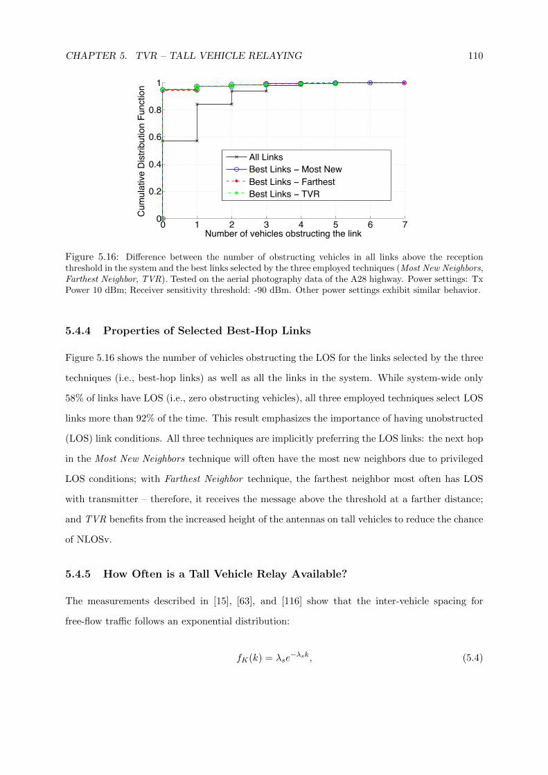
CHAPTER 5. TVR – TALL VEHICLE RELAYING 110
0 1 2 3 4 5 6 70
0.2
0.4
0.6
0.8
1
Number of vehicles obstructing the link
Cum
ulat
ive
Dis
tribu
tion
Func
tion
All LinksBest Links − Most NewBest Links − FarthestBest Links − TVR
Figure 5.16: Difference between the number of obstructing vehicles in all links above the receptionthreshold in the system and the best links selected by the three employed techniques (Most New Neighbors,Farthest Neighbor, TVR). Tested on the aerial photography data of the A28 highway. Power settings: TxPower 10 dBm; Receiver sensitivity threshold: -90 dBm. Other power settings exhibit similar behavior.
5.4.4 Properties of Selected Best-Hop Links
Figure 5.16 shows the number of vehicles obstructing the LOS for the links selected by the three
techniques (i.e., best-hop links) as well as all the links in the system. While system-wide only
58% of links have LOS (i.e., zero obstructing vehicles), all three employed techniques select LOS
links more than 92% of the time. This result emphasizes the importance of having unobstructed
(LOS) link conditions. All three techniques are implicitly preferring the LOS links: the next hop
in the Most New Neighbors technique will often have the most new neighbors due to privileged
LOS conditions; with Farthest Neighbor technique, the farthest neighbor most often has LOS
with transmitter – therefore, it receives the message above the threshold at a farther distance;
and TVR benefits from the increased height of the antennas on tall vehicles to reduce the chance
of NLOSv.
5.4.5 How Often is a Tall Vehicle Relay Available?
The measurements described in [15], [63], and [116] show that the inter-vehicle spacing for
free-flow traffic follows an exponential distribution:
fK(k) = λse−λsk, (5.4)
CHAPTER 5. TVR – TALL VEHICLE RELAYING 111
where λs is the inverse of the average inter-vehicle spacing in meters. For a certain ratio γ of tall
vehicles (0 ≤ γ ≤ 1), we have the following inter-vehicle spacing distribution for tall vehicles:
fK(k) = γλse−γλsk. (5.5)
To calculate the probability PT of there being at least one tall vehicle relay within a certain
average communication range R, we calculate the complement of the probability of having zero
tall vehicles within R:
PT = 1− Pr(k ≥ R) (5.6)
= FK(R)
= 1− e−γλsR,
where FK(·) is the Cumulative Distribution Function (CDF) of the inter-vehicle spacing between
tall vehicles. It has to be noted that, in real situations, R is going to be a variable that is
dependent on many factors (transmission power, road surroundings, etc.), including the vehicle
density, since the increased vehicular density will decrease the transmission range, as shown
in [16]. Therefore, we consider R as an average communication range for which the value can be
determined from experimental data such as that in Fig. 5.8. However, for the employed TVR
technique we are not interested in the existence of a tall vehicle within the entire R; rather,
we are interested in a distance interval [R − xmax, R], where xmax is calculated as described in
eq. 5.2 and eq. 3 and xmax ≤ R. Therefore, we have the following probability of having at least
one tall vehicle relay within [R− xmax, R]:
PT [R−xmax,R] = PT [0,xmax] (5.7)
= 1− Pr(k > xmax)
= FK(xmax)
= 1− e−γλsxmax ,
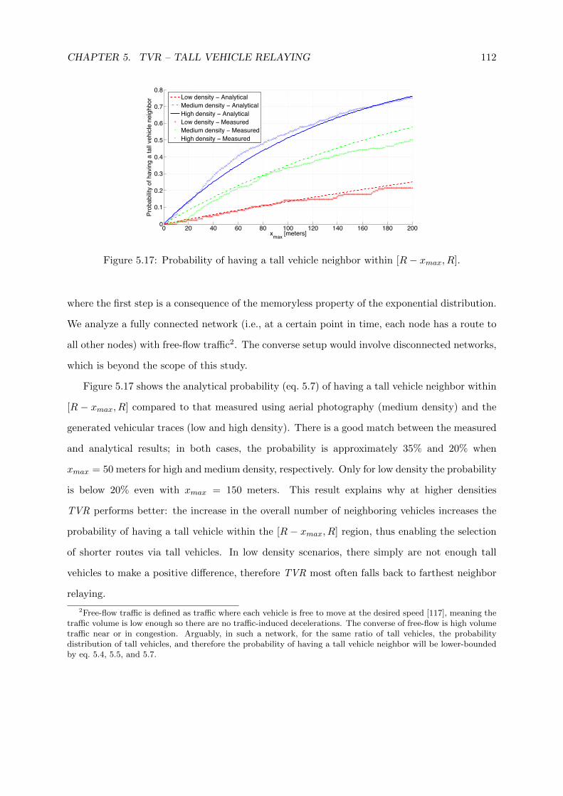
CHAPTER 5. TVR – TALL VEHICLE RELAYING 112
0 20 40 60 80 100 120 140 160 180 2000
0.1
0.2
0.3
0.4
0.5
0.6
0.7
0.8
xmax [meters]
Prob
abilit
y of
hav
ing
a ta
ll ve
hicl
e ne
ighb
or
Low density − AnalyticalMedium density − AnalyticalHigh density − AnalyticalLow density − MeasuredMedium density − MeasuredHigh density − Measured
Figure 5.17: Probability of having a tall vehicle neighbor within [R− xmax, R].
where the first step is a consequence of the memoryless property of the exponential distribution.
We analyze a fully connected network (i.e., at a certain point in time, each node has a route to
all other nodes) with free-flow traffic2. The converse setup would involve disconnected networks,
which is beyond the scope of this study.
Figure 5.17 shows the analytical probability (eq. 5.7) of having a tall vehicle neighbor within
[R − xmax, R] compared to that measured using aerial photography (medium density) and the
generated vehicular traces (low and high density). There is a good match between the measured
and analytical results; in both cases, the probability is approximately 35% and 20% when
xmax = 50 meters for high and medium density, respectively. Only for low density the probability
is below 20% even with xmax = 150 meters. This result explains why at higher densities
TVR performs better: the increase in the overall number of neighboring vehicles increases the
probability of having a tall vehicle within the [R − xmax, R] region, thus enabling the selection
of shorter routes via tall vehicles. In low density scenarios, there simply are not enough tall
vehicles to make a positive difference, therefore TVR most often falls back to farthest neighbor
relaying.
2Free-flow traffic is defined as traffic where each vehicle is free to move at the desired speed [117], meaning thetraffic volume is low enough so there are no traffic-induced decelerations. The converse of free-flow is high volumetraffic near or in congestion. Arguably, in such a network, for the same ratio of tall vehicles, the probabilitydistribution of tall vehicles, and therefore the probability of having a tall vehicle neighbor will be lower-boundedby eq. 5.4, 5.5, and 5.7.
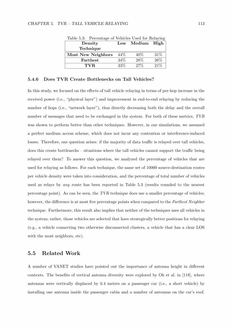
CHAPTER 5. TVR – TALL VEHICLE RELAYING 113
Table 5.3: Percentage of Vehicles Used for RelayingDensity Low Medium High
Technique
Most New Neighbors 44% 40% 31%
Farthest 34% 28% 26%
TVR 33% 27% 21%
5.4.6 Does TVR Create Bottlenecks on Tall Vehicles?
In this study, we focused on the effects of tall vehicle relaying in terms of per-hop increase in the
received power (i.e., “physical layer”) and improvement in end-to-end relaying by reducing the
number of hops (i.e., “network layer”), thus directly decreasing both the delay and the overall
number of messages that need to be exchanged in the system. For both of these metrics, TVR
was shown to perform better than other techniques. However, in our simulations, we assumed
a perfect medium access scheme, which does not incur any contention or interference-induced
losses. Therefore, one question arises: if the majority of data traffic is relayed over tall vehicles,
does this create bottlenecks – situations where the tall vehicles cannot support the traffic being
relayed over them? To answer this question, we analyzed the percentage of vehicles that are
used for relaying as follows. For each technique, the same set of 10000 source-destination routes
per vehicle density were taken into consideration, and the percentage of total number of vehicles
used as relays by any route has been reported in Table 5.3 (results rounded to the nearest
percentage point). As can be seen, the TVR technique does use a smaller percentage of vehicles;
however, the difference is at most five percentage points when compared to the Farthest Neighbor
technique. Furthermore, this result also implies that neither of the techniques uses all vehicles in
the system; rather, those vehicles are selected that have strategically better positions for relaying
(e.g., a vehicle connecting two otherwise disconnected clusters, a vehicle that has a clear LOS
with the most neighbors, etc).
5.5 Related Work
A number of VANET studies have pointed out the importance of antenna height in different
contexts. The benefits of vertical antenna diversity were explored by Oh et al. in [118], where
antennas were vertically displaced by 0.4 meters on a passenger car (i.e., a short vehicle) by
installing one antenna inside the passenger cabin and a number of antennas on the car’s roof.
CHAPTER 5. TVR – TALL VEHICLE RELAYING 114
Both parking lot and on-road experiments were conducted using IEEE 802.11a radios operating
in the 5.2 GHz frequency band. While mainly focusing on mitigating the negative effects of
ground reflections rather than dealing with vehicular obstructions, the results show that the
vertical diversity increases the effective communication range by more than 100 meters in certain
scenarios. Kaul et al. reported a similar study in [31], with a focus on determining the single best
location for an antenna in a passenger car. By performing parking lot and on-road experiments
using IEEE 802.11a radios operating in the 5.2 GHz frequency band, the center of the roof was
found to be the best overall position, with significant variation in reception patterns when the
antenna was displaced horizontally and vertically. On the other hand, two simulation studies
based on detailed ray-optical channel models (Reichardt et al. in [119] and Kornek et al. in [120])
indicate that antenna positions other than those on the roof (e.g., on side mirrors) can be
preferable in certain scenarios.
With respect to Vehicle-to-Infrastructure (V2I) links and the impact of antenna placement,
Paier et al. in [121] performed experiments which showed significantly better results with a
road-side unit (RSU) that was placed above the height of the tallest vehicles. Placing the RSUs
higher up results in a more reliable communication channel, which is particularly important for
safety related applications. Since the RSU radio design is similar to the on-board unit (OBU)
radios in vehicles, this finding suggests that the same applies for V2V communication; i.e.,
placing the antennas on taller vehicles is likely to result in improved radio channel. A similar
study was reported in [122], where the authors analyzed the performance of a downlink between
an RSU and an OBU installed in a vehicle. Antenna heights and traffic had a severe impact
on the downlink performance, and the authors pointed out that “shadowing effects caused by
trucks lead to a strongly fluctuating transmission performance, particularly for settings with
long packet lengths and higher speeds.” This reinforces the findings reported by Meireles et
al. in [16], where high losses were observed when obstructing vehicles were present between
communicating vehicles.
Regarding the performance analysis and modeling of LOS and non-LOS (NLOS) Tan et
al. in [33] performed V2V and V2I measurements in urban, rural, and highway environments at
5.9 GHz. The results point out significant differences with respect to delay spread and Doppler
shift in case of LOS and NLOS channels (NLOS was often induced by trucks obstructing the
LOS). The paper distinguishes LOS and NLOS communication scenarios by coarsely dividing
CHAPTER 5. TVR – TALL VEHICLE RELAYING 115
the overall obstruction levels. Similarly, Otto et al. in [14] performed V2V experiments in the
2.4 GHz frequency band in an open road environment and reported a significantly worse signal
reception during a heavy traffic, rush hour period in comparison to a no traffic, late night period.
In the WINNER project [123], a series of 5.3 GHz wireless experiments were performed with a
stationary base station and a moving node. The results were then used to derive channel models
for use in simulation. Higher antenna heights were found to be beneficial to communication: the
higher the antenna, the lower the path loss exponent. Several other experimental studies and
surveys discuss potential impact of vehicles on the channel quality: [1, 8, 9, 13,34,36,38,91].
Many relay selection metrics have been proposed for vehicular networks. The most common
can be divided into: 1) hop-count metrics (e.g., [124]); 2) received power metrics (e.g., [114]);
3) metrics based on geographic characteristics such as vehicle position, direction, or map infor-
mation, etc. (e.g., [125], [126]); and 4) vehicular density based metrics (e.g., [63]). Combination
of two or more of these metrics is also common in the literature. We have shown that relay-
ing messages over tall vehicles is beneficial in terms of the hop count metrics (TVR results in
fewer hops, particularly in dense vehicular networks) and received power metrics (tall vehicles
exhibit higher received power, PDR, and communication range). Apart from our preliminary
study reported in [69], to the best of our knowledge, none of the existing studies proposed uti-
lizing the information about the type and height of vehicles to improve the performance of V2V
communication.
5.6 Conclusions
We have determined the benefits of utilizing the height of vehicles to enable more efficient V2V
communication. We have shown that using knowledge about vehicle type/height to appropriately
select the next hop vehicle consistently results in increased effective communication range and
larger per-hop message reachability. Through both experiments and simulations that use a
validated model, we have shown that tall vehicles are significantly better relay candidates than
short vehicles when tall vehicles are within a certain distance of the farthest vehicle. Selecting
tall vehicles in such situations results in a higher received signal power, increased packet delivery
ratio, and larger effective communication range.
Furthermore, we characterized the properties of preferred next hops in an experimental set-
CHAPTER 5. TVR – TALL VEHICLE RELAYING 116
ting and by evaluating three relay techniques through large-scale simulations. Both experiments
and simulations showed that, when available, LOS links are preferred, regardless of the specific
environment or relaying technique. However, since the distinction between LOS and NLOS links
is not straightforward at the transmitter, we propose the tall vehicle relay (TVR) technique,
which increases the likelihood of having a LOS link. We have shown that by selecting tall instead
of farthest vehicles, TVR outperforms other techniques in terms of the number of hops to reach
the destination, which in turn reduces the end-to-end delay. Therefore, the farthest neighbor
metric might not be the best solution for selecting the next-hop relay where heterogeneous vehi-
cle types exist (i.e., tall and short). The type of potential relay candidate can play an important
role in deciding which next hop to select. Additionally, since TVR increases the received power
level and reduces hop count, it can be used to improve performance of existing routing protocols
by adding binary information on the type of vehicle (tall or short).
It is important to note that our findings can be used to enhance different types of routing
protocols, be it unicast [127, 128], broadcast [129, 130], geocast [126] or multicast [131]. On
highways, trucks and other tall commercial vehicles can be used as moving hotspots that relay
the messages between the shorter vehicles. In urban environments, public transportation vehicles
such as buses and streetcars can be used for the same purpose.
Chapter 6
Conclusion
The main goals of this thesis were to realistically and efficiently model the vehicle-to-vehicle
(V2V) channel and to design protocols that improve V2V communication. Towards this goal,
we started by performing an extensive set of experiments in order to set up the “ground truth”
regarding the following: 1) the impact of vehicular obstructions on inter-vehicle communication;
2) the impact of static objects (buildings and foliage); and 3) the performance characteristics
of different vertical antenna displacements. The measurements confirmed our hypothesis that
vehicles have a significant impact on signal propagation. Next, using the insights from mea-
surements, we designed a computationally efficient model that enables realistic modeling of the
impact of vehicles. Then, in order to enable simulating the channel in areas where static ob-
jects play an important role (e.g., urban and suburban areas), we introduced an efficient and
simplified geometry-based model that incorporates the effects of both vehicles and static objects
(namely, buildings and foliage) in terms of large-scale propagation effects (shadowing) as well
as small-scale (multipath fading). The model exhibits realistic behavior as validated using the
measurements. At the same time, the model is computationally efficient and requires minimum
geographic descriptors (namely, outlines of the modeled objects) that are readily available. This
makes it suitable for implementation in large scale, discrete-event VANET simulators. Finally,
in order to alleviate the shadowing effects caused by vehicles, we proposed a technique that
selects tall vehicles (e.g., buses, trucks) as next-hop relays where appropriate. The technique
improves communication performance in terms of the number of hops, end-to-end delay, and
effective communication range.
117
CHAPTER 6. CONCLUSION 118
6.1 Contributions
The main contributions of this thesis are as follows.
• Experimental evaluation of the impact of vehicular obstructions on inter-
vehicle communication. We characterized in detail the impact that LOS-obstructing
vehicles have on inter-vehicle communication in terms of received power, packet delivery
rate, and effective communication range by performing extensive measurements in different
environments (open space, highway, suburban, urban, parking lot).
• Model for incorporating vehicles as obstacles in channel models. We present a
model that accounts for vehicles as three-dimensional obstacles and takes into account their
impact on the line of sight obstruction, received signal power, and packet reception rate.
The model is based on the empirically derived vehicle dimensions, accurate vehicle posi-
tioning, and realistic mobility patterns. We validate the model against measurements and
it exhibits realistic propagation characteristics while maintaining manageable complexity.
• Computationally efficient, geometry-based, validated channel model for vehic-
ular communications. The model incorporates both static objects (buildings, foliage)
and mobile (vehicles on the road). It requires minimum geographic information: 1) In-
formation about the location of the vehicles on the road; and 2) Information about the
outline of static objects. We validate the model against measurements and show that it
successfully captures both the large-scale propagation effects as well as fading in different
environments (highway, urban, suburban, open space).
• Tall Vehicle Relaying technique. We performed an experimental study to determine
the benefits of using tall vehicles as next-hop relays. The results showed that selecting tall
vehicles is beneficial in terms of higher power at the receiver, smaller number of hops to
reach the destination, and increased per-hop communication range. Based on these results,
we proposed a technique that improves the inter-vehicle communication by selecting tall
vehicles (e.g., buses, trucks) as next-hop relays. The technique improves communication
performance by reducing the number of hops needed to reach the destination and increasing
the effective communication range.
CHAPTER 6. CONCLUSION 119
6.2 Future Work
The following are possible directions in which the work done in this thesis could be extended.
• Currently, we assume that the terrain is flat. With mainly flat terrains, this simplification
does not have a significant bearing on the results. For locations with significant elevation
changes, the model can be adapted so that the elevation is included, provided such data
is sufficiently accurate. To this end, we will explore using publicly available topography
data from sources such as Global Digital Elevation Model (http://asterweb.jpl.nasa.
gov/gdem.asp) and Shuttle Radar Topography Mission (http://wiki.openstreetmap.
org/wiki/SRTM).
• We limit the discussion to single antenna systems at both the transmitter and the re-
ceiver, with a note that the extension of the model to multiple antenna systems can be
incorporated through techniques such as the one presented by Reichardt et al. in [132].
• Interference from other nearby communicating pairs can be introduced using our model.
By simulating multiple communication sessions between nearby pairs of vehicles using the
developed model, the following can be evaluated: 1) the signal to interference ratio (SIR);
2) the impact on channel access (e.g., channel availability, back-off times, etc.); and 3) the
effect of interference on the upper layers of the protocol stack.
Bibliography
[1] D. Dhoutaut, A. Regis, and F. Spies, “Impact of radio propagation models in vehicular
ad hoc networks simulations,” VANET 06: Proceedings of the 3rd international workshop
on Vehicular ad hoc networks, pp. 69–78, 2006.
[2] J. Koberstein, S. Witt, and N. Luttenberger, “Model complexity vs. better parameter
value estimation: comparing four topography-independent radio models,” in Simutools
’09: Proceedings of the 2nd International Conference on Simulation Tools and Techniques,
ICST, Brussels, Belgium, 2009, pp. 1–8.
[3] D. Kotz, C. Newport, R. S. Gray, J. Liu, Y. Yuan, and C. Elliott, “Experimental evaluation
of wireless simulation assumptions,” in Proc. ACM MSWiM ’04. New York, NY, USA:
ACM, 2004, pp. 78–82.
[4] F. Bai, T. Elbatt, G. Hollan, H. Krishnan, and V. Sadekar, “Towards characterizing
and classifying communication-based automotive applications from a wireless networking
perspective,” 1st IEEE Workshop on Automotive Networking and Applications (AutoNet),
2006.
[5] M. Boban and T. T. V. Vinhoza, “Modeling and simulation of vehicular networks: Towards
realistic and efficient models,” in Mobile Ad-Hoc Networks: Applications. InTech, January
2011.
[6] C.-X. Wang, X. Cheng, and D. I. Laurenson, “Vehicle-to-vehicle channel modeling and
measurements: Recent advances and future challenges,” IEEE Communications Magazine,
vol. 47, no. 11, pp. 96–103, November 2009.
120

BIBLIOGRAPHY 121
[7] A. Molisch, F. Tufvesson, J. Karedal, and C. Mecklenbrauker, “Propagation aspects of
vehicle-to-vehicle communications - an overview,” in IEEE Radio and Wireless Sympo-
sium, 2009. RWS ’09., Jan. 2009, pp. 179 –182.
[8] D. Matolak and Q. Wu, “Vehicle-to-vehicle channels: Are we done yet?” in IEEE GLOBE-
COM Workshops, 2009, pp. 1 –6.
[9] D. Matolak, “Channel modeling for vehicle-to-vehicle communications,” IEEE Communi-
cations Magazine, vol. 46, no. 5, pp. 76 –83, may 2008.
[10] A. J. Goldsmith, Wireless Communications. Cambridge University Press, 2006.
[11] T. S. Rappaport, Wireless Communications: Principles and Practice. Prentice Hall, 1996.
[12] J. Maurer, T. Fugen, T. Schafer, and W. Wiesbeck, “A new inter-vehicle communications
(IVC) channel model,” in IEEE Vehicular Technology Conference, 2004, VTC2004-Fall,
September 2004, pp. 9–13.
[13] “Vehicle safety communications project, final report,” U.S. Department of Transportation,
NHTSA, Crash Avoidance Metrics Partnership, Tech. Rep. DOT HS 810 591, 2006.
[14] J. Otto, F. Bustamante, and R. Berry, “Down the block and around the corner the impact
of radio propagation on inter-vehicle wireless communication,” in 29th IEEE International
Conference on Distributed Computing Systems, ICDCS ’09., June 2009, pp. 605–614.
[15] M. Boban, T. T. V. Vinhoza, J. Barros, M. Ferreira, and O. K. Tonguz, “Impact of
vehicles as obstacles in vehicular ad hoc networks,” IEEE Journal on Selected Areas in
Communications, vol. 29, no. 1, pp. 15–28, January 2011.
[16] R. Meireles, M. Boban, P. Steenkiste, O. K. Tonguz, and J. Barros, “Experimental study
on the impact of vehicular obstructions in VANETs,” in IEEE Vehicular Networking Con-
ference (VNC 2010), Jersey City, NJ, USA, December 2010, pp. 338–345.
[17] H. Masui, T. Kobayashi, and M. Akaike, “Microwave path-loss modeling in urban line-of-
sight environments,” IEEE Journal on Selected Areas in Communications, vol. 20, no. 6,
pp. 1151–1155, Aug 2002.
[18] “JiST/SWANS homepage.” [Online]. Available: http://jist.ece.cornell.edu/
BIBLIOGRAPHY 122
[19] “Network Simulator 2.” [Online]. Available: http://nsnam.isi.edu/nsnam/index.php/
Main Page
[20] “Network Simulator 3.” [Online]. Available: www.nsnam.org
[21] “Qualnet.” [Online]. Available: http://www.qualnet.com
[22] J. Klosowski, M. Held, J. Mitchell, H. Sowizral, and K. Zikan, “Efficient collision detection
using bounding volume hierarchies of k-DOPs,” IEEE Transactions on Visualization and
Computer Graphics, vol. 4, no. 1, pp. 21 –36, January 1998.
[23] “IEEE Draft Standard IEEE P802.11p/D9.0,” Tech. Rep., July 2009.
[24] L. Cheng, B. E. Henty, D. D. Stancil, F. Bai, and P. Mudalige, “Mobile vehicle-to-vehicle
narrow-band channel measurement and characterization of the 5.9 ghz dedicated short
range communication (DSRC) frequency band,” IEEE Journal on Selected Areas in Com-
munications, vol. 25, no. 8, pp. 1501–1516, Oct. 2007.
[25] J. Andersen, T. Rappaport, and S. Yoshida, “Propagation measurements and models for
wireless communications channels,” IEEE Communications Magazine, vol. 33, no. 1, pp.
42–49, Jan 1995.
[26] F. J. Martinez, C. K. Toh, J.-C. Cano, C. T. Calafate, and P. Manzoni, “A survey and
comparative study of simulators for vehicular ad hoc networks (VANETs),” Wireless Com-
munications and Mobile Computing, vol. 11, no. 7, pp. 813 – 828, July 2011.
[27] “Car blueprints database.” [Online]. Available: http://carblueprints.info
[28] A. Festag, R. Baldessari, W. Zhang, L. Le, A. Sarma, and M. Fukukawa, “CAR-2-X
communication for safety and infotainment in Europe,” NEC Technical Journal, vol. 3,
no. 1, 2008.
[29] “IEEE Draft Standard IEEE P802.11p,” Tech. Rep., June 2010.
[30] G. Combs et al., “Wireshark-network protocol analyzer.” [Online]. Available:
http://www.wireshark.org
BIBLIOGRAPHY 123
[31] S. Kaul, K. Ramachandran, P. Shankar, S. Oh, M. Gruteser, I. Seskar, and T. Nadeem,
“Effect of antenna placement and diversity on vehicular network communications,” in 4th
Annual IEEE Communications Society Conference on Sensor, Mesh and Ad Hoc Commu-
nications and Networks, SECON ’07, june 2007, pp. 112–121.
[32] S. Takahashi, A. Kato, K. Sato, and M. Fujise, “Distance dependence of path loss for
millimeter wave inter-vehicle communications,” in Proc. IEEE 58th Vehicular Technology
Conference (VTC 2003-Fall), vol. 1, Oct. 2003, pp. 26–30.
[33] I. Tan, W. Tang, K. Laberteaux, and A. Bahai, “Measurement and analysis of wireless
channel impairments in DSRC vehicular communications,” in IEEE International Confer-
ence on Communications, ICC ’08., May 2008, pp. 4882–4888.
[34] A. Paier, J. Karedal, N. Czink, H. Hofstetter, C. Dumard, T. Zemen, F. Tufvesson,
A. Molisch, and C. Mecklenbrauker, “Car-to-car radio channel measurements at 5 GHz:
Pathloss, power-delay profile, and delay-Doppler spectrum,” in 4th International Sympo-
sium on Wireless Communication Systems, ISWCS 2007., Oct. 2007, pp. 224–228.
[35] I. Sen and D. Matolak, “Vehicle-Vehicle Channel Models for the 5-GHz Band,” IEEE
Transactions on Intelligent Transportation Systems, vol. 9, no. 2, pp. 235–245, June 2008.
[36] M. Jerbi, P. Marlier, and S. M. Senouci, “Experimental assessment of V2V and I2V com-
munications,” in Proc. IEEE Internatonal Conference on Mobile Adhoc and Sensor Sys-
tems (MASS 2007), Oct. 2007, pp. 1–6.
[37] H. Wu, M. Palekar, R. Fujimoto, R. Guensler, M. Hunter, J. Lee, and J. Ko, “An empirical
study of short range communications for vehicles,” in Proc. of the 2nd ACM International
workshop on Vehicular ad hoc networks, 2005, pp. 83–84.
[38] D. Matolak, I. Sen, W. Xiong, and N. Yaskoff, “5 GHz wireless channel characterization for
vehicle to vehicle communications,” in Proc. IEEE Military Communications Conference
(MILCOM 2005), October 2005, pp. 3016–3022.
[39] G. Acosta-Marum and M. Ingram, “Six time- and frequency-selective empirical channel
models for vehicular wireless LANs,” IEEE Vehicular Technology Magazine, vol. 2, no. 4,
pp. 4 –11, December 2007.
BIBLIOGRAPHY 124
[40] M. Boban, T. T. V. Vinhoza, O. K. Tonguz, and J. Barros, “Seeing is believing – enhancing
message dissemination in vehicular networks through visual cues,” IEEE Communications
Letters, vol. 16, no. 2, pp. 238–241, Feb. 2012.
[41] T. Nadeem, S. Dashtinezhad, C. Liao, and L. Iftode, “Trafficview: traffic data dissemina-
tion using car-to-car communication,” SIGMOBILE Mob. Comput. Commun. Rev., vol. 8,
no. 3, pp. 6–19, 2004.
[42] W. Chen and S. Cai, “Ad hoc peer-to-peer network architecture for vehicle safety com-
munications,” IEEE Communications Magazine, vol. 43, no. 4, pp. 100–107, April 2005.
[43] O. K. Tonguz and M. Boban, “Multiplayer games over vehicular ad hoc networks: A new
application,” Ad Hoc Networks, vol. 8, no. 5, pp. 531 – 543, 2010.
[44] D. R. Choffnes and F. E. Bustamante, “An integrated mobility and traffic model for
vehicular wireless networks,” in VANET ’05: Proceedings of the 2nd ACM international
workshop on Vehicular ad hoc networks. New York, NY, USA: ACM, 2005, pp. 69–78.
[45] “NCTUns 6.0 network simulator and emulator.” [Online]. Available: http://nsl.csie.nctu.
edu.tw/nctuns.html
[46] A. Glassner, Ed., An Introduction to Ray Tracing. Academic Press, 1989.
[47] G. Acosta and M. Ingram, “Model development for the wideband expressway vehicle-to-
vehicle 2.4 GHz channel,” in IEEE Wireless Communications and Networking Conference,
2006. WCNC 2006., vol. 3, April 2006, pp. 1283–1288.
[48] Y. Zang, L. Stibor, G. Orfanos, S. Guo, and H.-J. Reumerman, “An error model for inter-
vehicle communications in highway scenarios at 5.9ghz,” in PE-WASUN ’05: Proceedings
of the 2nd ACM international workshop on Performance evaluation of wireless ad hoc,
sensor, and ubiquitous networks. New York, NY, USA: ACM, 2005, pp. 49–56.
[49] H. Kim and H.-S. Lee, “Accelerated three dimensional ray tracing techniques using ray
frustums for wireless propagation models,” Progress In Electromagnetics Research, PIER,
no. 96, pp. 595–611, 2009.
BIBLIOGRAPHY 125
[50] J. Karedal, F. Tufvesson, N. Czink, A. Paier, C. Dumard, T. Zemen, C. Mecklenbrauker,
and A. Molisch, “A geometry-based stochastic MIMO model for vehicle-to-vehicle commu-
nications,” IEEE Transactions on Wireless Communications, vol. 8, no. 7, pp. 3646–3657,
July 2009.
[51] A. Paier, J. Karedal, N. Czink, H. Hofstetter, C. Dumard, T. Zemen, F. Tufvesson,
C. Mecklenbrauker, and A. Molisch, “First results from car-to-car and car-to-infrastructure
radio channel measurements at 5.2 GHz,” in IEEE 18th International Symposium on Per-
sonal, Indoor and Mobile Radio Communications, 2007. PIMRC 2007., September 2007,
pp. 1–5.
[52] X. Cheng, C.-X. Wang, D. I. Laurenson, S. Salous, and A. V. Vasilakos, “An adap-
tive geometry-based stochastic model for non-isotropic mimo mobile-to-mobile channels,”
IEEE Transactions on Wireless Communications, vol. 8, no. 9, pp. 4824–4835, 2009.
[53] R. W. Rothery, “Car following models,” In Trac Flow Theory, 1992.
[54] O. K. Tonguz, W. Viriyasitavat, and F. Bai, “Modeling urban traffic: a cellular automata
approach,” IEEE Communications Magazine, vol. 47, no. 5, pp. 142–150, 2009.
[55] O. Shih, H. Tsai, H. Lin, and A. Pang, “A rule-based mixed mobility model for cars and
scooters (poster),” in IEEE Vehicular Networking Conference (VNC), 2011, pp. 198–205.
[56] ITU-R, “Propagation by diffraction,” International Telecommunication Union Radiocom-
munication Sector, Geneva, Recommendation P.526, February 2007.
[57] J. D. Parsons, The Mobile Radio Propagation Channel. John Wiley & Sons, 2000.
[58] J. Epstein and D. W. Peterson, “An experimental study of wave propagatin at 850MC,”
Proceedings of the IRE, vol. 41, no. 5, pp. 595–611, 1953.
[59] J. Deygout, “Multiple knife-edge diffraction of microwaves,” IEEE Transactions on An-
tennas and Propagation, vol. 14, no. 4, pp. 480–489, 1966.
[60] C. L. Giovaneli, “An analysis of simplified solutions for multiple knife-edge diffraction,”
IEEE Transactions on Antennas and Propagation, vol. 32, no. 3, pp. 297–301, 1984.
BIBLIOGRAPHY 126
[61] McCasland, W T, “Comparison of Two Techniques of Aerial Photography for Application
in Freeway Traffic Operations Studies,” Photogrammetry and Aerial Surveys, 1965.
[62] M. Ferreira, H. Conceicao, R. Fernandes, and O. K. Tonguz, “Stereoscopic aerial pho-
tography: an alternative to model-based urban mobility approaches,” in Proceedings of
the Sixth ACM International Workshop on VehiculAr Inter-NETworking (VANET 2009).
ACM New York, NY, USA, 2009.
[63] N. Wisitpongphan, F. Bai, P. Mudalige, V. Sadekar, and O. K. Tonguz, “Routing in sparse
vehicular ad hoc wireless networks,” IEEE Journal on Selected Areas in Communications,
vol. 25, no. 8, pp. 1538–1556, Oct. 2007.
[64] “Associacao Automovel de Portugal.” [Online]. Available: http://www.acap.pt/
[65] “Automotive Technical Data and Specifications.” [Online]. Available: http://www.
carfolio.com/
[66] A. Papoulis, Probability, Random Variables and Stochastic Processes, 2nd ed. McGraw-
Hill, 1984.
[67] Z. Wang, E. Tameh, and A. Nix, “Statistical peer-to-peer channel models for outdoor
urban environments at 2 ghz and 5 ghz,” in IEEE Vehicular Technology Conference, 2004.
VTC2004-Fall. 2004, vol. 7, Sept. 2004, pp. 5101–5105 Vol. 7.
[68] “Standard Specification for Telecommunications and Information Exchange Between
Roadside and Vehicle Systems - 5GHz Band Dedicated Short Range Communications
(DSRC) Medium Access Control (MAC) and Physical Layer (PHY) Specifications,” ASTM
E2213-03, Sep. 2003.
[69] M. Boban, R. Meireles, J. Barros, O. K. Tonguz, and P. Steenkiste, “Exploiting the height
of vehicles in vehicular communication,” in IEEE Vehicular Networking Conference (VNC
2011), Amsterdam, The Netherlands, November 2011, pp. 284–291.
[70] “DRIVE-IN (Distributed Routing and Infotainment through VEhicular Inter-
Networking).” [Online]. Available: http://drive-in.cmuportugal.org
BIBLIOGRAPHY 127
[71] M. Haklay and P. Weber, “OpenStreetMap: User-generated street maps,” IEEE Pervasive
Computing, vol. 7, no. 4, pp. 12–18, 2008.
[72] X. Wang, E. Anderson, P. Steenkiste, and F. Bai, “Improving the accuracy of environment-
specific vehicular channel modeling,” in Proceedings of the seventh ACM international
workshop on Wireless network testbeds, experimental evaluation and characterization,
WiNTECH ’12. New York, NY, USA: ACM, 2012, pp. 43–50.
[73] T. Blaschke, “Object based image analysis for remote sensing,” ISPRS Journal of Pho-
togrammetry and Remote Sensing, vol. 65, no. 1, pp. 2–16, 2010.
[74] “National Agriculture Imagery Program (NAIP).” [Online]. Available: http://www.fsa.
usda.gov/FSA/apfoapp?area=home&subject=prog&topic=nai
[75] H. J. Haverkort, “Results on geometric networks and data structures,” Ph.D. dissertation,
Utrecht University, 2004.
[76] A. Guttman, “R-trees: a dynamic index structure for spatial searching,” SIGMOD Rec.,
vol. 14, pp. 47–57, June 1984.
[77] Y. Theodoridis and T. Sellis, “A model for the prediction of R-tree performance,” in
Proceedings of the fifteenth ACM SIGACT-SIGMOD-SIGART symposium on Principles
of database systems, ser. PODS ’96. New York, NY, USA: ACM, 1996, pp. 161–171.
[78] M. de Berg, M. van Kreveld, M. Overmars, and O. Schwarzkopf, Computational Geometry
Algorithms and Applications. Springer-Verlag, 1997.
[79] J. Karedal, F. Tufvesson, T. Abbas, O. Klemp, A. Paier, L. Bernado and, and A. Molisch,
“Radio channel measurements at street intersections for vehicle-to-vehicle safety applica-
tions,” in IEEE Vehicular Technology Conference (VTC 2010-Spring), May 2010, pp. 1
–5.
[80] C. Sommer and F. Dressler, “Using the Right Two-Ray Model? A Measurement based
Evaluation of PHY Models in VANETs,” in 17th ACM International Conference on Mobile
Computing and Networking (MobiCom 2011), Poster Session. Las Vegas, NV: ACM,
September 2011.
BIBLIOGRAPHY 128
[81] T. Mangel, M. Michl, O. Klemp, and H. Hartenstein, “Real-world measurements of Non-
Line-of-Sight reception quality for 5.9 GHz IEEE 802.11p at intersections,” in Proceedings
of the Third international conference on Communication technologies for vehicles, ser.
Nets4Cars/Nets4Trains’11. Berlin, Heidelberg: Springer-Verlag, 2011, pp. 189–202.
[82] G. Durgin, T. Rappaport, and H. Xu, “Measurements and models for radio path loss and
penetration loss in and around homes and trees at 5.85 GHz,” IEEE Transactions on
Communications, vol. 46, no. 11, pp. 1484–1496, November 1998.
[83] J. Goldhirsh and W. J. Vogel, “Handbook of propagation effects for vehicular and personal
mobile satellite systems – overview of experimental and modeling results,” The Johns
Hopkins University, Applied Physics Laboratory and The University of Texas at Austin,
Electrical Engineering Research Laboratory, Tech. Rep. A2A-98-U-0-021 (APL), EERL-
98-12A (EERL), December 1998.
[84] F. Ulaby, M. Whitt, and M. Dobson, “Measuring the propagation properties of a forest
canopy using a polarimetric scatterometer,” IEEE Transactions on Antennas and Propa-
gation, vol. 38, no. 2, pp. 251 –258, feb 1990.
[85] B. Benzair, H. Smith, and J. Norbury, “Tree attenuation measurements at 1-4 GHz for
mobile radio systems,” in Sixth International Conference on Mobile Radio and Personal
Communications, December 1991, pp. 16–20.
[86] H. Anderson, “Building corner diffraction measurements and predictions using UTD,”
IEEE Transactions on Antennas and Propagation, vol. 46, no. 2, pp. 292 –293, February
1998.
[87] A. Abdi, J. Barger, and M. Kaveh, “A parametric model for the distribution of the angle of
arrival and the associated correlation function and power spectrum at the mobile station,”
IEEE Transactions on Vehicular Technology, vol. 51, no. 3, pp. 425–434, 2002.
[88] J. Kunisch and J. Pamp, “Wideband car-to-car radio channel measurements and model
at 5.9 GHz,” in IEEE Vehicular Technology Conference, 2008. VTC 2008-Fall, September
2008, pp. 1 –5.
BIBLIOGRAPHY 129
[89] J. Karedal, N. Czink, A. Paier, F. Tufvesson, and A. Molisch, “Path loss modeling for
vehicle-to-vehicle communications,” IEEE Transactions on Vehicular Technology, vol. 60,
no. 1, pp. 323–328, January 2011.
[90] O. Landron, M. Feuerstein, and T. Rappaport, “A comparison of theoretical and empirical
reflection coefficients for typical exterior wall surfaces in a mobile radio environment,”
IEEE Transactions on Antennas and Propagation, vol. 44, no. 3, pp. 341–351, March
1996.
[91] T. Abbas, J. Karedal, F. Tufvesson, A. Paier, L. Bernado, and A. Molisch, “Directional
analysis of vehicle-to-vehicle propagation channels,” in 73rd IEEE Vehicular Technology
Conference (VTC Spring), May 2011, pp. 1–5.
[92] A. Paier, J. Karedal, N. Czink, C. Dumard, T. Zemen, F. Tufvesson, A. Molisch, and
C. Mecklenbrauker, “Characterization of vehicle-to-vehicle radio channels from measure-
ments at 5.2 GHz,” Wireless Personal Communications, vol. 50, pp. 19–32, 2009.
[93] F. Neves, A. Cardote, R. Moreira, and S. Sargento, “Real-world evaluation of IEEE 802.11p
for vehicular networks,” in Proceedings of the Eighth ACM international workshop on
Vehicular inter-networking (VANET ’11). New York, NY, USA: ACM, 2011, pp. 89–90.
[94] E. Giordano, R. Frank, G. Pau, and M. Gerla, “CORNER: a realistic urban propagation
model for VANET,” in Proceedings of the 7th international conference on Wireless on-
demand network systems and services (WONS), 2010, pp. 57–60.
[95] P. Paschalidis, K. Mahler, A. Kortke, M. Peter, and W. Keusgen, “Pathloss and multipath
power decay of the wideband car-to-car channel at 5.7 GHz,” in IEEE Vehicular Technology
Conference (VTC Spring), May 2011, pp. 1–5.
[96] T. Abbas, F. Tufvesson, and J. Karedal, “Measurement based shadow fading model for
vehicle-to-vehicle network simulations,” arXiv preprint arXiv:1203.3370v2, 2012.
[97] J. Fernandez, K. Borries, L. Cheng, B. Kumar, D. Stancil, and F. Bai, “Performance
of the 802.11p physical layer in vehicle-to-vehicle environments,” IEEE Transactions on
Vehicular Technology, vol. 61, no. 1, pp. 3 –14, January 2012.
BIBLIOGRAPHY 130
[98] B. Chazelle and L. Guibas, “Visibility and intersection problems in plane geometry,”
Discrete & Computational Geometry, vol. 4, no. 1, pp. 551–581, 1989.
[99] S. Molnar, M. Cox, D. Ellsworth, and H. Fuchs, “A sorting classification of parallel ren-
dering,” IEEE Computer Graphics and Applications, vol. 14, no. 4, pp. 23–32, 1994.
[100] L. Luo, M. Wong, and L. Leong, “Parallel implementation of R-trees on the GPU,” in
17th IEEE Asia and South Pacific Design Automation Conference (ASP-DAC), 2012, pp.
353–358.
[101] T. Mangel, O. Klemp, and H. Hartenstein, “A validated 5.9 GHz Non-Line-of-Sight path-
loss and fading model for inter-vehicle communication,” in 11th International Conference
on ITS Telecommunications (ITST), August 2011, pp. 75 –80.
[102] C. Sommer, D. Eckhoff, R. German, and F. Dressler, “A computationally inexpensive
empirical model of IEEE 802.11p radio shadowing in urban environments,” in Eighth In-
ternational Conference on Wireless On-Demand Network Systems and Services (WONS),
2011, pp. 84 –90.
[103] F. J. Martinez, C.-K. Toh, J.-C. Cano, C. T. Calafate, and P. Manzoni, “Realistic radio
propagation models (RPMs) for VANET simulations,” in Wireless Communications and
Networking Conference, 2009. WCNC 2009. IEEE, April 2009, pp. 1–6.
[104] H. Cozzetti, C. Campolo, R. Scopigno, and A. Molinaro, “Urban VANETs and hidden
terminals: evaluation through a realistic urban grid propagation model,” in IEEE In-
ternational Conference on Vehicular Electronics and Safety (ICVES), July 2012, pp. 93
–98.
[105] M. Sepulcre and J. Gozalvez, “Experimental evaluation of cooperative active safety appli-
cations based on V2V communications,” in Proceedings of the ninth ACM international
workshop on Vehicular inter-networking, systems, and applications, ser. VANET ’12. New
York, NY, USA: ACM, 2012, pp. 13–20.
[106] B. Gallagher, H. Akatsuka, and H. Suzuki, “Wireless communications for vehicle safety:
radio link performance and wireless connectivity methods,” IEEE Vehicular Technology
Magazine, vol. 1, no. 4, pp. 4 –24, December 2006.
BIBLIOGRAPHY 131
[107] J. Gozalvez, M. Sepulcre, and R. Bauza, “IEEE 802.11p vehicle to infrastructure commu-
nications in urban environments,” IEEE Communications Magazine, vol. 50, no. 5, pp.
176 –183, May 2012.
[108] P.-J. Wang, C.-M. Li, and H.-J. Li, “Influence of the shadowing on the information trans-
mission distance in inter-vehicle communications,” in IEEE International Symposium on
Personal, Indoor and Mobile Radio Communications (PIMRC), September 2009, pp. 3015
–3019.
[109] K. Bullington, “Radio propagation for vehicular communications,” IEEE Transactions on
Vehicular Technology, vol. 26, no. 4, pp. 295 – 308, nov 1977.
[110] M. Boban, R. Meireles, J. Barros, P. A. Steenkiste, and O. K. Tonguz, “TVR - tall vehicle
relaying in vehicular networks,” IEEE Transactions on Mobile Computing, vol. 99, p. 1,
2013.
[111] M. Ferreira, H. Conceicao, R. Fernandes, and O. Tonguz, “Urban connectivity analy-
sis of VANETs through stereoscopic aerial photography,” in IEEE Vehicular Technology
Conference Fall (VTC 2009-Fall), Sept. 2009, pp. 1–3.
[112] “802.11p Line of Sight Experiment website.” [Online]. Available: http://drive-in.
cmuportugal.org/los
[113] M. Torrent-Moreno, P. Santi, and H. Hartenstein, “Distributed fair transmit power ad-
justment for vehicular ad hoc networks,” in 3rd Annual IEEE Communications Society
Conference on Sensor and Ad Hoc Communications and Networks, SECON ’06, vol. 2,
sept. 2006, pp. 479 –488.
[114] V. Naumov, R. Baumann, and T. Gross, “An evaluation of inter-vehicle ad hoc networks
based on realistic vehicular traces,” in MobiHoc ’06: Proceedings of the 7th ACM inter-
national symposium on Mobile ad hoc networking and computing, New York, NY, USA,
2006, pp. 108–119.
[115] N. Wisitpongphan, O. K. Tonguz, J. Parikh, P. Mudalige, F. Bai, and V. Sadekar, “Broad-
cast storm mitigation techniques in vehicular ad hoc networks,” IEEE Wireless Commu-
nications, vol. 14, no. 6, pp. 84–94, Dec. 2007.
BIBLIOGRAPHY 132
[116] F. Bai and B. Krishnamachari, “Spatio-temporal variations of vehicle traffic in VANETs:
facts and implications,” in VANET ’09: Proceedings of the sixth ACM international work-
shop on VehiculAr InterNETworking. New York, NY, USA: ACM, 2009, pp. 43–52.
[117] A. D. May, Traffic flow fundamentals. Prentice Hall, 1990.
[118] S. Oh, S. Kaul, and M. Gruteser, “Exploiting vertical diversity in vehicular channel envi-
ronments,” in IEEE 20th International Symposium on Personal, Indoor and Mobile Radio
Communications, Sept. 2009, pp. 958 –962.
[119] L. Reichardt, T. Fugen, and T. Zwick, “Influence of antennas placement on car to car
communications channel,” in 3rd European Conference on Antennas and Propagation,
EuCAP 2009., march 2009, pp. 630–634.
[120] D. Kornek, M. Schack, E. Slottke, O. Klemp, I. Rolfes, and T. K andrner, “Effects of
antenna characteristics and placements on a vehicle-to-vehicle channel scenario,” in IEEE
International Conference on Communications Workshops, May 2010, pp. 1–5.
[121] A. Paier, D. Faetani, and C. Mecklenbrauker, “Performance evaluation of IEEE 802.11p
physical layer infrastructure-to-vehicle real-world measurements,” in Proceedings of IS-
ABEL 2010, Rome, Italy, November 2010.
[122] A. Paier, R. Tresch, A. Alonso, D. Smely, P. Meckel, Y. Zhou, and N. Czink, “Average
downstream performance of measured IEEE 802.11p infrastructure-to-vehicle links,” in
IEEE International Conference on Communications Workshops, 2010, may 2010, pp. 1
–5.
[123] D. S. Baum et al., “IST-2003-507581 WINNER I, D5.4, Final report on link level and
system level channel models,” Information Society Technologies, Tech. Rep., 2005.
[124] V. Namboodiri, M. Agarwal, and L. Gao, “A study on the feasibility of mobile gateways
for vehicular ad-hoc networks,” in VANET ’04: Proceedings of the 1st ACM international
workshop on Vehicular ad hoc networks. New York, NY, USA: ACM, 2004, pp. 66–75.
[125] V. Naumov and T. Gross, “Connectivity-aware routing (CAR) in vehicular ad-hoc net-
works,” in 26th IEEE International Conference on Computer Communications, INFO-
COM 2007., May 2007, pp. 1919–1927.
BIBLIOGRAPHY 133
[126] C. Lochert, H. Hartenstein, J. Tian, H. Fussler, D. Hermann, and M. Mauve, “A routing
strategy for vehicular ad hoc networks in city environments,” Proceedings of the IEEE
Intelligent Vehicles Symposium, 2003., pp. 156–161, June 2003.
[127] M. Boban, G. Misek, and O. K. Tonguz, “What is the best achievable QoS for unicast
routing in VANETs?” in IEEE GLOBECOM, 3rd Workshop on Automotive Networking
and Applications (AutoNet), New Orleans, LA, USA, November 2008, pp. 1–10.
[128] M. Boban, O. K. Tonguz, and J. Barros, “Unicast communication in vehicular ad hoc
networks: a reality check,” IEEE Communications Letters, vol. 13, no. 12, pp. 995–997,
December 2009.
[129] W. Viriyasitavat, O. K. Tonguz, and F. Bai, “UV-CAST: an urban vehicular broadcast
protocol,” IEEE Communications Magazine, vol. 49, no. 11, pp. 116–124, November 2011.
[130] O. K. Tonguz, N. Wisitpongphan, and F. Bai, “DV-CAST: A distributed vehicular broad-
cast protocol for vehicular ad hoc networks,” IEEE Wireless Communications, vol. 17,
no. 2, pp. 47–57, April 2010.
[131] M. Kihl, M. Sichitiu, T. Ekeroth, and M. Rozenberg, “Reliable geographical multicast
routing in vehicular ad-hoc networks,” in Wired/Wireless Internet Communications, ser.
Lecture Notes in Computer Science, F. Boavida, E. Monteiro, S. Mascolo, and Y. Kouch-
eryavy, Eds. Springer Berlin / Heidelberg, 2007, vol. 4517, pp. 315–325.
[132] L. Reichardt, J. Pontes, W. Wiesbeck, and T. Zwick, “Virtual drives in vehicular commu-
nication,” IEEE Vehicular Technology Magazine, vol. 6, no. 2, pp. 54 –62, june 2011.
Related Documents