Planning and Operation of DSTATCOM in Electrical ... - ethesis

Planning and Operation of DSTATCOM in Electrical Distribution Systems

Joseph Sanam

Department of Electrical Engineering National Institute of Technology Rourkela

Planning and Operation of DSTATCOM

in Electrical Distribution Systems

Dissertation Submitted in partial fulfillment

of the requirements for the degree of

Doctor of Philosophy

in

Electrical Engineering

by

Joseph Sanam (Roll Number: 513EE1016)

Under the supervision of

Prof. Anup Kumar Panda

And

Prof. Sanjib Ganguly

June 2017

Department of Electrical Engineering

National Institute of Technology Rourkela, India

Department of Electrical Engineering

National Institute of Technology Rourkela 16th Sept 2017

Certificate of Examination

Roll Number: 513EE1016

Name: Joseph Sanam

Title of Dissertation: Planning and Operation of DSTATCOM in Electrical Distribution

Systems

We the below signed, after checking the dissertation mentioned above and the official record book(s) of the student, hereby state our approval of the dissertation submitted in partial fulfillment of the requirements of the degree of Doctor of Philosophy in Electrical Engineering at National Institute of Technology Rourkela. We are satisfied with the volume, quality, correctness, and originality of the work.

Prof. Monalisa Pattnaik Member, DSC

Prof. S.K.Behera Member, DSC

External Examiner

Prof. K. B. Mohanty (Chairman, DSC)

Jitendriya Kumar Satapathy Head of the Department

Pro. Sanjib Ganguly Co- Supervisor

Prof. Anup Kumar Panda Principal Supervisor

Prof. Subrata Karmakar Member, DSC

Department of Electrical Engineering National Institute of Technology Rourkela

16th Sept 2017

Supervisor's Certificate

This is to certify that the work presented in this dissertation entitled “Planning and

Operation of DSTATCOM in Electrical Distribution Systems” submitted by Joseph

Sanam, Roll Number 513EE1016, is a record of original research carried out by him under

our supervision and guidance in partial fulfillment of the requirements of the degree of

Doctor of Philosophy in Electrical Engineering. Neither this dissertation nor any part of it

has been submitted for any degree or diploma to any institute or university in India or

abroad.

Dr. Sanjib Ganguly (Co-Supervisor)

Prof. Anup Kumar Panda (Principal Supervisor)

Assistant Professor Department of Electronics and Electrical

Engineering Indian Institute of Technology

Guwahati, Assam, India, Pin Code: 781039

Professor Department of Electrical Engineering

National Institute of Technology Rourkela, Orissa, and India

Pin Code: 769008

Declaration of Originality

I, Joseph Sanam, Roll Number 513EE1016 hereby declare that this dissertation entitled

“Planning and Operation of DSTATCOM in Electrical Distribution Systems” represents

my original work carried out as a doctoral student of NIT Rourkela and, to the best of my

knowledge, it contains no material previously published or written by another person, nor

any material presented for the award of any other degree or diploma of NIT Rourkela or

any other institution. Any contribution made to this research by others, with whom I have

worked at NIT Rourkela or elsewhere, is explicitly acknowledged in the dissertation. The

works of other authors cited in this dissertation have been duly acknowledged under the

section ''Bibliography''. I have also submitted my original research records to the doctoral

scrutiny committee for evaluation of my dissertation.

I am fully aware that in case of any non-compliance detected in the future, the Senate

of NIT Rourkela may withdraw the degree awarded to me on the basis of the present

dissertation.

16th Sept 2017

NIT Rourkela Joseph Sanam

Acknowledgement

I express my profound gratitude to Prof. Anup Kumar Panda, Department of Electrical

Engineering, NIT Rourklea and Prof. Sanjib Ganguly, Department of Electronics and

Electrical Engineering, IIT Guwahati for accepting as a student in the Power systems group

and suggesting me the research topic. I am deeply indebted for their continuous support

and encouragement given during the research work. I consider myself fortunate to have

worked under their guidance. I am indebted to them for providing all official and

laboratory facilities.

I am grateful to the Director, Prof. S.K. Sarangi and Prof. Jitendriya Kumar Satpathy,

Head of Electrical Engineering Department, National Institute of Technology, Rourkela,

for their kind support and concern regarding my academic requirements.

I gratefully thank to my Doctoral Scrutiny Committee members, Prof. Kanungo Barada

Mohanty, Prof. Subrata Karmakar , Prof. Monalisa Pattnaik and Prof. S.K. Behera, for

their valuable suggestions and contributions of this dissertation. I express my thankfulness

to the faculty and staff members of the Electrical Engineering Department for their

continuous encouragement and suggestions.

At this point, I wish to specifically emphasize my gratitude for all the help and

encouragement I received from my supervisor Prof. Anup Kumar Panda Prof. Sanjib

Ganguly. During communication of the journal publications, their guidance and insight

gave me encouragement to proceed with confidence towards publishing in the reputed

journals of this work. Also, personally at hard times my supervisors provided great moral

support.

I am especially indebted to all my colleagues in the power systems group. I would like

to thank my colleagues Mr. Damodar Panigrahi and Mr. Chaduvula Hemanth for their help

and support throughout my research work.

I am especially grateful to Power Electronics Laboratory staff Mr. Rabindra Nayak. I

would also like to thank my friends, Mr. Hhussain, Mr. Padarabinda Samal, Mr. Srihari

Nayak, Mr. Maheswar Behra, Mr. Nobby George, Mr. Kondal Rao, Mr. K. Vinay Sagar,

Mr. Siva Kumar, Mr. Muralidhar Killi, Mr. Nishanth Patnaik, Mr. Mrutyunjay, Mr.

Trilochan, Mr. Pratap, Mr. Ashish, Mr. Kishore thakre, Ms. Sneha Prava Swain, Ms.

Jyothi, Ms. Richa Patnaik, Ms. C. Aditi, Ms. Snigtha, and Ms. Ranjeeta Patel etc. for

extending their technical and personal support.

I express my deep sense of gratitude and reverence to my beloved father Sri. Samuel

Sanam, Mother Smt. Ratnamma Sanam, Brothers Mr. Timothy Sanam, Mr. Immanuel

Sanam. Mr. Mephibosheth Sanam, Mr. Benjamin Sanam, Sister Ms. Sarah Sanam, sister-

in-laws, Hadassa Sanam, and Sharon Sanam. I can never forget my father-in-law Sri.

Phiroz Kumar and mother-in law Smt. Snehalata Roshni Soy because their help and

support during my Ph.D work is so great, and they helped me lot all the time no matter

what difficulties I encountered. I especially thank my wife Jolly Rachel Sanam, her

support, encouragement, patience and unwavering love, provided strength to focus on the

work. I would like to express my greatest admiration to all my family members and

relatives for their positive encouragement that they showered on me throughout this

research work. Without my family’s sacrifice and support, this research work would not

have been possible. It is a great pleasure for me to acknowledge and express my

appreciation to all my well-wishers for their understanding, relentless supports, and

encouragement during my research work. Last but not the least, I wish to express my

sincere thanks to all those who helped me directly or indirectly at various stages of this

work.

Above all, I would like to thank The Almighty God for the wisdom and perseverance

that he has been bestowed upon me during this research work, and indeed, throughout my

life.

16th Sept, 2017 Joseph Sanam NIT Rourkela Roll Number: 513EE1016

Contents

Certificate of Examination

Supervisor's Certificate

Declaration of Originality

Acknowledgement

Contents

List of figures

List of tables

Abbreviations

Notations

Abstract

Chapter 1: Introduction 1

1.1. Brief description of Electric Power System 1

1.1.1. Networks involved in electric power system 3

1.1.2. Planning, and operation of electric power systems 6

1.2. Overview of Electrical Distribution Systems 8

1.2.1. Primary distribution 10

1.2.2. Secondary distribution 11

1.2.3. Two-wire D.C. distribution system 11

1.2.4. Three-wire D.C. distribution system 13

1.2.5. Radial distribution system 14

1.2.6. Loop distribution system 15

1.2.7. Network distribution system 16

1.2.8. Classification of buses in distribution systems 17

1.3. Research background on electrical distribution systems 18

1.4. Motivation 21

1.5. Objectives of thesis 22

1.6. Work done 22

1.7. Thesis organization 23

Chapter 2: Phase angle model of DSTATCOM and its Incorporation in FBS algorithm

25

2.1. Introduction 25

2.2. DSTATCOM in the proposed approach 26

2.2.1. What is DSTATCOM? 26

2.2.2. Components involved in DSTATCOM design 26

2.2.3. Working principle of DSTATCOM 27

2.2.4. Limitations in the operation of DSTATCOM 32

2.2.5. Advantages of DSTATCOM 32

2.3. The new phase angle Model of DSTATOCM 33

2.4.

Incorporation of phase angle model of DSTATCOM in FBS algorithm

37

2.4.1. FBS Load flow technique 37

2.4.2 Incorporation of a new phase angle model of DSTATCOM in FBS Load flow algorithm

40

2.5. Conclusion 44

Chapter 3: Reactive Power Compensation in Radial Distribution Systems with the Optimal Phase Angle Injection Model of Single Distribution STATCOM

45

3.1. Introduction 45

3.2. Optimal allocation of DSTATCOM in RDS using exhaustive search algorithm

45

3.2.1. Objective Function 46

3.2.1.1. Voltage constraint 46

3.2.1.2. Thermal constraint 46

3.2.2. Exhaustive search optimization method (ESM) 47

3.2.3. 69-bus RDS 49

3.2.3.1. DSTATCOM allocation strategy 49

3.2.3.2. Simulation Result 49

3.2.4. 30-bus RDS 52

3.2.4.1. DSTATCOM placement scheme 52

3.2.4.2. Simulation Results 52

3.3. DSTATCOM Allocation Using DE 55

3.3.1. DE: an overview 55

3.3.2. Proposed Solution Strategy Using DE 57

3.3.3. Proposed DE algorithm 58

3.4. Simulation Results 59

3.4.1. Results of Exhaustive Search 61

3.4.2. Results of DSTATCOM allocation using DE 64

3.4.3. Comparative results with some of the previous works 66

3.5. Conclusion 67

Chapter 4: Optimization of Planning Cost of Distribution Systems with the Optimal Placement and Sizing of DSTATCOM Using Differential Evolution Algorithm

68

4.1. Introduction 68

4.2. Importance of Planning 68

4.3. Planning for Industrial Distribution Systems 69

4.4. Mathematical problem formulation 70

4.3.1. Objective function (F) 70

4.3.2. Real power loss 72

4.3.3. Present worth factor (PWF) analysis 72

4.3.4. TNP/Savings 73

4.5. Constraints 73

4.6. Solution Strategy Using DEA 78

4.7. Simulation results 79

4.7.1. Impact of DSTATCOM allocation 81

4.7.2. Analysis of power loss reduction 84

4.7.3. Analysis of planning cost 91

4.7.4. Analysis of ELC 93

4.7. Conclusion 94

Appendix 95

Chapter 5 Optimal Phase Angle injection for Reactive Power Compensation of Distribution Systems with the Allocation of Multiple DSTATCOM and DG

98

5.1. Introduction 98

5.2. Multiple DSTATCOM allocation 98

5.2.1. Proposed Solution Strategy Using DE 99

5.2.2. Simulation Results 100

5.3. Allocation of DSTATCOM and DG 105

5.3.1. Importance of DSTATCOM and DG allocation in RDS 105

5.3.2. Problem Formulation 106

5.3.3. Integration of DSTATCOM and DG 107

5.3.4. Analysis of Simulation Results 110

5.3.4.1. Power loss reduction 111

5.3.4.2. Benefit analysis of the proposed approach 113

5.4. Conclusion 114

Chapter 6 Conclusion and Future Scope 115

6.1. Conclusion 115

6.2. Future Scope 116

References 117

Thesis Disseminations 132

Author’s Biography 133

List of Figures

S. No Figure. No Figure Tittle Page.

No 1 1.1 The block diagram of electric power system 1

2 1.2 A simple layout of electric power system 2

3 1.3 The line diagram of radial distribution system 8

4 1.4 Two-wire D.C. distribution system 12

5 1.5 Three-wire D.C. distribution system 13

6 1.6 The typical diagram of radial distribution system 14

7 1.7 The typical diagram of loop distribution system 15

8 1.8 The typical diagram of Network distribution system 17

9 2.1 A simple line diagram of an electric line connected between two consecutive voltage sources

27

10 2.2 A simple Radial distribution line with the allocation of DSTATCOM

29

11 2.3 The time diagram of DSTATCOM voltage and current in inductive mode of operation (absorption of Q)

30

12 2.4 The time diagram of DSTATCOM voltage and current in capacitive mode of operation (generation of Q)

31

13 2.5 Two successive buses of DN drawn as a single line diagram 33

14 2.6 Phasor diagram for the network shown in Fig.2.5 33

15 2.7 Single line diagram with a DSTATCOM placed at bus n+1 34

16 2.8 Phasor diagram for the network shown in Fig.2.7 35

17 2.9 Simple RDS considered for FBS load flow studies 38

18 2.10 Forward backward sweep algorithm flow chart integrating the DSTATCOM mathematical model

43

19 3.1 Active power loss after installation of DSTATCOM in RDS

51

20 3.2 Voltage magnitude in different cases with DSTATCOM at bus 61

51

21 3.3 Figure.3.3: VA rating required for DSTATCOM in different locations of RDS

51

22 3.4 Variation of power loss with increment of DSTATCOM size in each node

53

23 3.5 DSTATCOM size corresponding to minimum power loss 53

24 3.6 minimum power loss in each node due to integration of DSTATCOM

54

25 3.7 minimum node voltage due to the integration of DSTATCOM

54

26 3.8 Voltage magnitude with DSTATCOM at node 5 55

27 3.9 Flow chart of proposed DE algorithm 60

28 3.10 Variation of active power loss with increment of phase angle β'n+1 in each bus

61

29 3.11 DSTATCOM rating in kVAr corresponding to minimum active and reactive power loss

62

30 3.12 Minimum active power loss in each node due to DSTATCOM

62

31 3.13 Minimum bus voltage due to DSTATCOM integration 63

32 3.14 Minimum reactive power loss in each node due to DSTATCOM

63

33 3.15 Minimum active power loss of each generation with single DSTATCOM allocation

64

34 3.16 Mean active power loss of each generation with DSTATCOM allocation

65

35 3.17 Mean reactive power loss of each generation with DSTATCOM allocation

65

36 4.1 Time Duration Curve 70

37 4.2 A typical string for DEA 75

38 4.3 Typical IEEE 30-bus DN 76

39 4.4 Typical IEEE 33-bus DN 77

40 4.5 Typical IEEE 69-bus DN 77

41 4.6 Cost analysis per annum 82

42 4.7 Cost analysis of total PH of DSTATCOM installation scheme

82

43 4.8 Total scheme mean cost of IEEE 30-bus distribution network

83

44 4.9 Total scheme mean cost of IEEE 33-bus network 83

45 4.10 Total scheme mean cost of IEEE 69-bus distribution network

84

46 4.11 Power loss at different loads with DSTATCOM at each bus of IEEE 30-bus distribution network

85

47 4.12 Minimum bus voltage at different loads with DSTATCOM at each bus of IEEE 30-bus distribution network

86

48 4.13 Voltage magnitude at various loads with DSTATCOM at bus 5 of IEEE 30-bus distribution network

86

49 4.14 Size of DSTATCOM at each bus of IEEE 30-bus distribution network at various loads

87

50 4.15 Power loss at different loads with DSTATCOM at each bus of IEEE 33-bus distribution network

87

51 4.16 Minimum bus voltage at various loads with DSTATCOM at each bus of IEEE 33-bus distribution network

88

52 4.17 Voltage magnitude at various loads with DSTATCOM at bus 30 of IEEE 33-bus distribution network

88

53 4.18 The size of DSTATCOM at each bus of IEEE 33-bus distribution network at different loads

89

54 4.19 Power loss at different loads with DSTATCOM at each bus of IEEE 69-bus distribution network

89

55 4.20 Minimum bus voltage at various loads with DSTATCOM at each bus of IEEE 69-bus distribution network

90

56 4.21 Voltage magnitude at various loads with DSTATCOM at bus 61 of IEEE 69-bus distribution network

90

57 4.22 Size of DSTATCOM at each bus of IEEE 69-bus distribution network at different loads

91

58 5.1 A typical string for DE for the allocation multiple DSTATCOMs

100

59 5.2 Power loss corresponding to the best solution with single DSTATCOM allocation

102

60 5.3 Mean power loss of each generation with multiple DSTATCOM allocation

102

61 5.4 Voltage profile with and without allocation of multiple DSTATCOM

103

62 5.5 Flow chart of load flow algorithm with ESM 109

63 5.6 Variation of power loss with increment of DG size in each node

111

64 5.7 Minimum power loss in each node due to integration of DSTATCOM or DG

112

65 5.8 DSTATCOM or DG size corresponding to minimum power loss

112

66 5.9 Voltage magnitude with DSTATCOM and DG at node 5 113

List of Tables S. No Table.

No Table Tittle Page.

No

1 2.1 FBS load flow algorithm 41

2 3.1 A generalized pseudocode for the exhaustive search algorithm

47

3 3.2 ESM Algorithm for proposed approach 48

4 3.3 Results obtained with DSTATCOM allocation at bus 61 50

5 3.4 Results obtained with DSTATCOM allocation at node 5 using exhaustive search

52

6 3.5 Parameters of DE algorithm 59

7 3.6 Comparative results with single DSTATCOM allocation 66

8 4.1 Constraints considered in proposed approach 75

9 4.2 Parameters of DEA for cost optimization problem 75

10 4.3 Load duration time and load level 78

11 4.4 Parameters of objective function 79

12 4.5 Comparative results of reactive power compensation with DSTATCOM for three load levels

80

13 4.6 Comparative results of annual cost of RDS with DSTATCOM installation without considering operational and maintenance cost of DSTATCOM

81

14 4.7 Results of total costs considering PWF for PH of DSTATCOM installation scheme ,including operational and maintenance cost of DSTATCOM

81

15 4.8 Comparison of TNP of proposed approach with the capacitor placement approaches

92

16 4.9 The solution obtained with proposed de algorithm in 50 run considering PWF for planning horizon including operational and maintenance cost of DSTATCOM

92

17 4.10 Comparison of convergence of mean curve of F 93

18 A Data of 33 bus DN 95

19 B Data of 69 bus DN 96

20 5.1 Parameters of DE algorithm for multiple DSTATCOM problem

100

21 5.2 Comparative results of multiple DSTATCOMs allocation 101

22 5.3 Reactive power compensation of RDS with the optimal allocation of multiple DSTATCOMs using DEA

104

23 5.4 ESM Algorithm for the allocation of DSTATCOM and DG 108

24 5.5 Results obtained after the allocation of single DSTATCOM or DG

110

25 5.6 Results obtained with the allocation of DG and DSTATCOM simultaneously

110

List of Abbreviations S. No Acronym Abbreviation

1 DSTATCOM Distribution Static Synchronous Compensator

2 DEA Differential Evolution Algorithm

3 ELC Energy loss cost

4 PWF Present worth factor

5 DN Distribution networks

6 DISCO Distribution companies

7 DG Distribution generators

8 NPV Net present value

9 PV Photovoltaic

10 ACO Ant colony optimization

11 O&M Operating and maintenance

12 FBS Forward-Backward sweep

13 VSC Voltage source converter

14 PCC Point of common coupling

15 TNP Total net profit

16 PH Planning horizon

17 RDN Radial distribution network

18 DG Distributed generation

19 ESM Exhaustive search method

20 AVR Automatic voltage regulator

21 DFACTS Distribution network flexible AC transmission

22 UPQC Unified power flow conditioner

23 SSSC Static synchronous series compensator

24 RDS Radial distribution systems

25 DVR Dynamic voltage restorer

26 NP Number of population

27 D String dimension

28 CR Crossover rate

29 F Scaling factor

30 TPC Total planning cost

31 PV Photovoltaic

32 ACO Ant colony otimization

33 O&M Operational and maintenance

34 kVAr Kilo volt ampere

35 kW Kilo watt

36 IA Immune algorithm

37 CPU Central processing unit

38 PSO Particle swarm optimization

39 TG Target vector

40 MUT Mutant vector

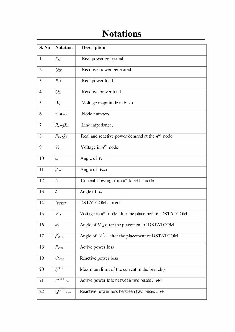
Notations S. No Notation Description

1 PGi Real power generated

2 QGi Reactive power generated

3 PLi Real power load

4 QLi Reactive power load

5 |Vi| Voltage magnitude at bus i

6 n, n+1 Node numbers

7 Rn+jXn Line impedance,

8 Pn, Qn Real and reactive power demand at the nth node

9 Vn Voltage in nth node

10 αn Angle of Vn

11 βn+1 Angle of Vn+1

12 In Current flowing from nth to n+1th node

13 δ Angle of In

14 IDSTAT DSTATCOM current

15 V 'n Voltage in nth node after the placement of DSTATCOM

16 αn' Angle of V 'n after the placement of DSTATCOM

17 β'n+1 Angle of V 'n+1 after the placement of DSTATCOM

18 Ploss Active power loss

19 Qloss Reactive power loss

20 Ijmax Maximum limit of the current in the branch j.

21 Pi,i+1 loss Active power loss between two buses i, i+1

22 Qi,i+1 loss Reactive power loss between two buses i, i+1

23 Ri,i+1 loss Resistance between two buses i, i+1

24 Iline Line current

25 Iload Load current

26 Xi,i+1 loss Reactance between two buses i, i+1

27 Ce Energy cost per kWh

28 f21 Total initial capital investment cost the DSTATCOM

29 f22 Total operational cost of the DSTATCOM

30 f23 Total maintenance costs of the DSTATCOM

31 Tk Duration of time in kth load level

32 Cin Initial capital investment cost of DSTATCOM per kVAr

33 Cop Operational cost of the DSTATCOM per kWh

34 Cma DSTATCOM maintenance cost which in terms of the % of initial cost

35 QkDSTAT Size of the DSTATCOM placed at optimal location during kth

load level

36 kck Proportionality constant of kth load level

37 Active power loss during kth load level after DSTATCOM is installed

38 k

Load level

39 Ib (j) Line current of jth branch

40 Rb (j) Resistance of jth branch

41 Vimin Minimum limits of the voltage at bus number i

42 Vimax Maximum limits of the voltage at bus number i

k

DSTATlossP

Abstract In present day scenario, it is most essential to consider the maximum asset performance

of the power distribution systems to reach the major goals to meet customer demands. To

reach the goals, the planning optimization becomes crucial, aiming at the right level of

reliability, maintaining the system at a low total cost while keeping good power quality.

There are some problems encountered which are hindering the effective and efficient

performance of the distribution systems to maintain power quality. These problems are

higher power losses, poor voltage profile near to the end customers, harmonics in load

currents, sags and swells in source voltage etc. All these problems may arise due to the

presence of nonlinear loads, unpredictable loads, pulse loads, sensor and other energy

loads, propulsion loads and DG connections etc. Hence, in order to improve the power

quality of power distribution systems, it is required to set up some power quality mitigating

devices, for example, distribution static synchronous compensator (DSTATCOM),

dynamic voltage restorer (DVR), and unified power quality conditioner (UPQC) etc. The

goal of this project work is to devise a planning of optimal allocation of DSTATCOM in

distribution systems using optimization techniques so as to provide reactive power

compensation and improve the power quality.

Keywords: Distribution Systems; Power Loss; Voltage Profile; Forward- Backward

Load flow algorithm; Phase angle Model of DSTATCOM; Differential Evolution

Algorithms, Total Planning Cost; Total Net Profit; Planning Horizon; Present Worth

Factor etc.

1

Chapter 1

Introduction

1.1. Brief description of Electric Power System

An electric power system is a network of various electrical Components(equipment)

installed for the generation, transmission, distribution and utilization of electrical power.

Power system consists of alternators that are driven by prime movers, grid, substations,

transformers, circuit breakers, bus bars, and other auxiliary devices, etc. that are used to

transfer power from generating stations to load in most reliable, economical and efficient

manner [1] and [2].

Figure.1.1: The block diagram of electric power system

Fig. 1.1 signifies the block diagram of electric power system. In the block diagram, it

can be seen that the power system comprises the various stages of operations such as

generation, transmission, distribution, and utilization along with the measurement of the

monitoring system and protection system. The simple layout of the electric power system

is shown in Fig. 1.2.

Power System

Measurement and Monitoring System

Protection System

Generation

Transmission Distribution

Utilization

2

Figure.1.2: A simple layout of electric power system

11/132kV

G

Gen

erat

ion

Tra

nsm

issi

on

Dis

trib

utio

n

Util

izat

ion

Generating Station

Voltage is stepped up to 132kV/275kV/500kV etc.

Primary transmission

Very large consumers

132/33kV Voltage is stepped down to

33kV/66kV etc.

Receiving station

Secondary transmission Large consumers

33/11kV Voltage is stepped down to distribution level ‘11kV’

Sub station

Secondary distribution

Medium consumers/ Industrial consumers

11kV/400V Distribution transformer (Voltage step-down to

400V/230V)

Primary distribution

Smaller consumers/Residential consumers/Commercial consumers

3

In Fig.1.2, it is very clear that the power generated by generating stations flows through

four stages to reach consumer’s load such as generation, transmission, distribution and

utilization. The transmission of power low has two steps i.e. primary and secondary

transmission. Similarly, the distribution has two steps i.e. primary and secondary

distribution. The power generating stations are usually located at a dam site where hydro

energy is available, near a fuel source e.g. nuclear fuels such as uranium-235 or plutonium-

239 and thermal energy fuels such as coal, natural gas, wood waste, etc., according to the

availability of renewable energy sources such as solar, wind, rain, tides, waves, and

geothermal heat etc. and in lightly populated areas [3] and [4].

The electric power which is generated by generating stations is at a low voltage around

11kV to 33kV depending on the output power rating of the generator. This voltage is

stepped up to higher voltages such as 132kv or 275kV or 500kV etc. as shown in Fig. 1.2.

The voltage which is stepped up is connected to the transmission system. The transmission

system then will carry the electric power for long distances, now and then it flows through

international boundaries too through two stages i.e. primary and secondary transmission,

until it reaches the electric power distribution system. Very large loads are connected to

the primary transmission system [5] and [6]. After the primary transmission, the voltage

is stepped down to 132kV or 33kV and is connected to the receiving station where the

large loads are being fed through the secondary transmission system [7]. At the end of

secondary transmission, the power arrives the distribution system. In the distribution

system, the voltage is stepped down to the voltage level of utilization through primary end

secondary distribution system stages. The detailed discussion on distribution system is

given in section 1.2.

1.1.1. Networks involved in electric power system

As it is discussed in above section, the power flow in electric power system happens

through four stages to reach a consumer’s load. These four stages are comprised with the

combinatorial operation of various networks such as power grid, transmission network,

substation network, and distribution network, etc.

4

I. Power Grid: The power grid is an interconnected system of several generating stations

with the same relative frequency for delivering electricity from suppliers to

consumers. The power grid can also be called as the combined operation of

transmission and distribution systems. Power grid involves three things generating

stations, transmission lines, and distribution lines [8].

II. Transmission system: The network/system which carries the bulk amount of electric

power from generating stations to the distribution station and then to load station is

called as the transmission system [9].

III. Substation: Substation is the part of the power system where the high transmission

voltage is stepped down to lower distribution voltages suitable for the voltage levels

required for industrial, commercial and residential consumers. The substation can also

be called as the interconnection of two dissimilar transmission system voltages[10].

The substations are supervised and controlled using SCADA (supervisory control and

data acquisition). When the electric power generated by the generating station flows

to the consumer's load, it flows through various substations at different of voltages.

Hence, the substations are classified as follows [11]:

a) Transmission Substation

b) Distribution Substation

c) Collector Substations

d) Converter Substation

e) Switching Substation

f) Traction Substation

a) Transmission Substation

The substation which connects two or more than two transmission lines at one point

is nothing but transmission substation. This substation consists transformers to

transform voltage from one transmission line to another, capacitors to improve the

power factor, voltage controller to control the voltage at different frequencies,

phase shifting transformers which control the power stream between two power

systems that are adjacent to each other, and static VAR compensators. The large

transmission substations are constructed with, several circuit breakers, multiple

5

voltage levels and many numbers of control and protection and equipment

(SCADA systems, relays, current and voltage transformers) to transmit the electric

power to a large region in hectares [12].

b) Distribution Substation

The substation which transfers electric power from the transmission system to the

distribution system of a region or zone is nothing but distribution substation. The

voltages of this substation are medium voltage based on the size of the load area

and the customs of indigenous utility. The more details of the distribution

substations are given in section 1.2.

c) Collector Substation

The substation which is used in wind farm based distributed generations projects

is called as collector substation. This substation collects power from several wind

turbines and moves it to the transmission grid. The flow of power is in opposite

direction though it resembles a distribution substation. The collector substation

operates the voltage around 33kV or 35 kV only because of the economy of

construction. This voltage gets stepped up to the level of grid voltage by the

collector substation. These substations are also used in hydroelectric and thermal

power plants whose output power almost same. This substation can correct the

power factor and control the wind turbines etc [13].

d) Converter Substations

It’s a substation which converts the power from A.C. to D.C. and vice versa using

power electronic devices [14]. These substations are complex to operate but are

required for transmitting HVDC (high voltage direct current) or interconnection of

two A.C. networks or interconnection of non-synchronous networks. The main

equipment includes the capacitors, filters, reactors and valves. The valves of the

converter substations are located in the large transformers.

e) Switching Substation

The substation which operates the single voltage level without any transformer is

known as switching substation. The switching substation can also be called as the

switchyard and is connected to the power station directly or located just adjacent

6

to the power station. The switch yard has two sides in which one side is the

generator bus, and another side is the feeder bus. The power generated from the

power station is supplied to the generator bus through one side of the switchyard,

and the transmission lines take that power from the feeder bus through the other

side of the switch yard. Hence, the switch yard connects and disconnects the

transmission lines to and from the power station or other elements for switching

the current to parallelizing circuits or backup lines in case of maintenance or

failure, or new construction occurs, i.e., removing or adding transformers or

transmission lines or some other elements. So, the switching substation causes the

reliability of power supply [15].

f) Traction(railway) substation

Traction Substation is one which converts AC currents to DC currents to electrify

DC trains and AC currents to AC currents at the different frequencies to electrify

the AC trains. Hence the traction substations have the both the rectifier and inverter

circuits. However, the output frequency of inverter circuit to electrify the AC trains

is other than the that of the local(public) grid. If the railways operate their

generators and grid, then the traction substation will also work as converter

substation or transmission substation [16].

1.1.2. Planning, and operation of electric power systems

The planning, operation, and control of entire power systems are quite complex and

crucial task since it is a large system which involves four stages of operation such as the

generation, transmission, distribution, and utilization. There are two reasons why it is so

complex, firstly, the entire system must be operated in synchronism. Secondly, the many

various companies and organizations are involved in different portions of the entire system

where they are needed to be more responsible. Hence, the optimal planning, operation, and

control or power system are required to minimize the operational cost and delivering the

secure and reliable power to the consumers. The whole operation of the power system is

divided into three stages [17]-[20]:

a) Planning

7

b) Control

c) Accounting

a) Planning: The demand of the load varies in each hour, week, and month. As the

load varies, the generation of the power varies to meet the anticipated demand. The

generation fo the power depends on the availability of resources such as hydro

energy (Water head), thermal energy fuels, nuclear energy fuels and renewable

energy fuels. Hence, to meet the load demand in various periods of time, it is

required to plan(schedule) the resources optimally. The optimal

planning(scheduling) is nothing but the planning of resources, maintenance of

equipment and the start-up and shutdown of generating units over many hours,

weeks, and months [21].

b) Control: To respond the current demand of the load and some unexpected

equipment outages the real time control of the power system is necessary. The real

time control system helps to maintain the system security to avoid the disruptions

in power supply due to unexpected equipment outages (contingency) [22].

c) Accounting: Accounting is nothing but “after-the-fact accounting” which tracks

the sales and purchase of electrical energy among companies and organizations to

generate the bills. These bills are useful to forecast the power demand and the

corresponding requirement of generation fuels, also, to forecast the quality of

power so that the shunt and series compensating devices can be added to the system

to improve the power quality.

1.2. Overview of Electrical Distribution Systems

The electric power distribution system is the point where the power gets delivered from

the transmission system to the costumer’s Load (Utilization). The distribution system

starts from the third stage of power systems as shown in Fig.1.2. On arrival of power at

distribution systems from the secondary transmission, the voltage gets stepped down from

the level of transmission to the level of distribution voltage (medium voltage) i.e. 33kV or

11kV using step-down transformers. This medium voltage is then transferred to the

distribution transformers through the primary distribution system. Some consumer’s loads

8

such as medium loads or industrial loads that demand a large amount of power supply are

directly connected to the primary distribution systems or the sub-transmission systems.

After the primary distribution, the power enters into the distribution wiring through a

substation and then finally arrives the service location where the power stopped down to

the level of utilization at the voltage of 3.3kV or 400V or 230V which is called the

secondary distribution. The secondary distribution system feeds smaller loads or

commercial loads or residential loads [23]-[26].

Figure.1.3: The line diagram of radial distribution system

It can be understood from Figs 1.2 and 1.3 that the distribution substation has at least two

sub-transmission or transmission lines as input and the several feeders as output. The

distribution feeders run along the roads underground or overhead lines and carry the power

to the consumer’s load through the distribution transformers. Many at times the

distribution substations not only transforming the voltage but isolate faults in either

distribution or transmission systems. A simple line diagram of the radial distribution

system is shown in Fig.1.3. The transference of electric power from the transmission

system to the distribution system is done by using following equipment[27]-[31]:

a) Substation,

b) Transformers

c) Radial feeders,

d) Bus bar or node and

Step-down transformer

S

Radial Feeders Bus or Node

Radial Distributor

Sub Station

9

e) Radial distributor.

f) Service mains

g) Circuit breakers etc.

a) Substation: The system, which transfer’s power from the transmission system to

the distribution system of a zone or region is called as a substation. The consumer’s

loads except very large loads can not be connected directly to the main

transmission system since it is uneconomical. Hence, the substation is required to

be used to step down the voltage to a level, which is appropriate for local service

distribution.

b) Transformers: Transformers are located in distribution substation are used to step

down the voltages in transmission lines down to primary distribution voltages.

Important pieces of equipment that reduce the voltage of electricity from a high

level to a level that can be safely distributed to an area, or a residence/business.

c) Radial Feeder: It is a medium voltage line(conductor) used to delivers electric

power from a substation to consumer to small substations. The current in the

feeders remains constant since there is no tapping of current from the feeder. The

current carrying capacity has to be considered to design a feeder.

d) Switch: Control the flow of electricity and steer the current to the correct circuits.

It avoids the short circuits between circuits.

e) Busbar: A thick rigid bars of copper strips, which works as a common connection

between many circuits and splits the electric power off in multiple directions in

distribution lines.

f) Radial distributor: Radial distributor is a line (conductor), which distributes the

electric power from bus bar to the consumers along with a single path. The current

in the radial distributor is not constant since it taps the current at many locations

along its length. The voltage drop along its length is the main consideration while

designing a distributor.

g) Service Mains: It is a small line (cable) which carries power from distributor to the

terminals of the consumer’s load.

10

h) Circuit Breakers: A circuit breaker is an automatic electric switch which interrupts

the flow of current into the distribution substation from the transmission system

and distribution lines to protect distribution substation from the damage caused by

overload and short circuit currents when a fault occurs.

The electrical distribution system is broadly classified as follows: [32]-[36]

1. According to the nature of current:

a) A.C. distribution system: these are subclassified into two types

1). Primary distribution system

2). Secondary distribution system

b) D.C. distribution system: these are subclassified into two types

1). Two-wire DC distribution system

2). Three-wire DC distribution system

A.C. distribution system is more economical and simpler than D.C. distribution

system. Hence, in recent days, A.C. distribution systems are adopted universally.

2. According to the scheme of connection:

a) Radial distribution system

b) Loop distribution system

c) Network distribution system

3. According to the type of construction:

a) Overhead distribution system

b) Underground distribution system

1.1.1. Primary distribution

The primary distribution is one which supplies electric power to various substations per

a region or zone. These substations distribute 230 V of power directly to the consumer's

load. The primary distribution systems are operated at the voltages higher than the

secondary distribution system and handle the energy of the huge block. The voltage levels

of the primary distribution system depend on two factors, firstly, the amount of electric

power to be carried to the substation and secondly, the distance of the substation. The

voltage level of most of the primary distribution systems is ranged between 3.3 kV to

11

33 kV phase-to-phase and 2.4 kV to 20 kV phase-to-neutral. A single phase and three

phase power are drawn by the load from three-phase service. Distribution of Single-phase

power happens by primary distribution for light load motors.The primary distribution

system usually carried out by three phase three wire system because of the economic

considerations. The main advantage of primary distribution is, it distributes power directly

to the medium load consumers. Maximum service consumers are connected to the

transformers, which step down the distribution voltage to the mains(supply) voltage

utilized by interior and lighting wiring systems. The voltage of the primary distribution

systems varies according to the need of power supply to the load [37] and [38].

1.1.2. Secondary distribution

It is the part of an A.C. distribution systems which delivers the electrical energy from

primary distribution to the ultimate consumer’s utilization whose voltage is of 400V and

230V. It is the combination of several distribution substations fed by the primary

distribution system. The distribution substations are allocated nearer to the consumer’s

area or locality and comprise step down transformers. Each substation steps down the

voltage to 400V and delivers power to the load by a three phase, four-wire system. The

voltage between two phases is 400V and between phase and neutral is 230V. All single-

phase residential, commercial and smaller loads are connected between any phase and

neutral. However, the large electric motor loads, clothes dryers, and electric stoves are

connected between any two phases directly since the three-phase energy is extra capable

regarding power delivered per cable. It is necessary to provide a ground connection for the

consumer's equipment and the equipment maintained by the utility to shun the

consequences abnormal voltages that are occurred due to the occurrence of a fault in

distribution transformer and the fall of high voltage lines on the low voltage lines [39-40].

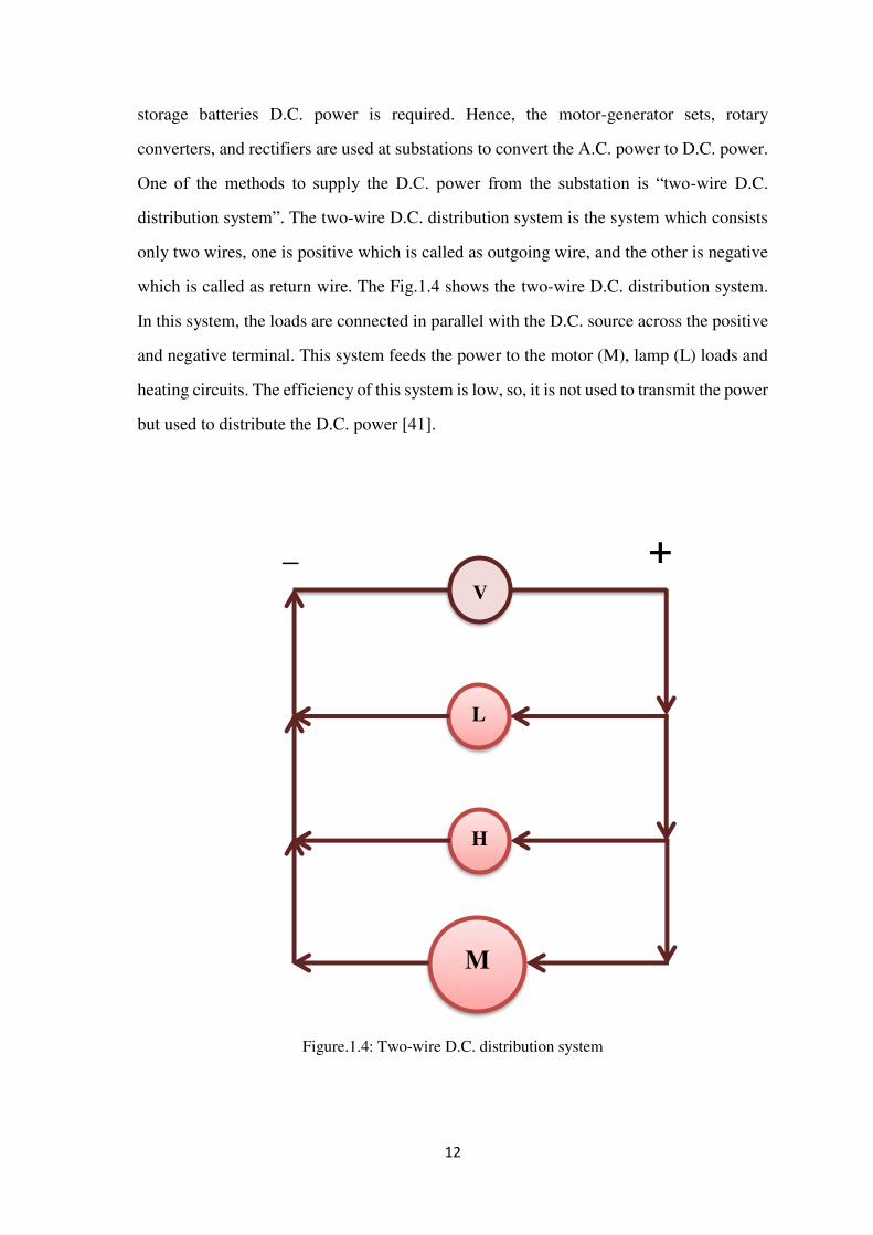
1.1.3. Two-wire D.C. distribution system

It is well known that nowadays, the electric power is virtually generated, transmitted

and distributed as A.C. because the magnitude of alternating voltage can be easily and

expediently changed using transformers. However, D.C. power is unequivocally required

for some applications. For example, for the variable speed D.C. motors, and the industrial

12

storage batteries D.C. power is required. Hence, the motor-generator sets, rotary

converters, and rectifiers are used at substations to convert the A.C. power to D.C. power.

One of the methods to supply the D.C. power from the substation is “two-wire D.C.

distribution system”. The two-wire D.C. distribution system is the system which consists

only two wires, one is positive which is called as outgoing wire, and the other is negative

which is called as return wire. The Fig.1.4 shows the two-wire D.C. distribution system.

In this system, the loads are connected in parallel with the D.C. source across the positive

and negative terminal. This system feeds the power to the motor (M), lamp (L) loads and

heating circuits. The efficiency of this system is low, so, it is not used to transmit the power

but used to distribute the D.C. power [41].

Figure.1.4: Two-wire D.C. distribution system

_ +

V

L

H

M

13

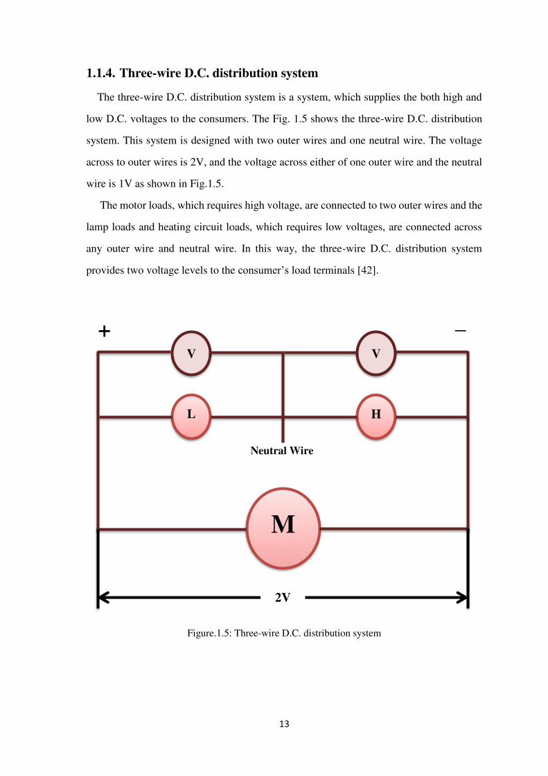
1.1.4. Three-wire D.C. distribution system

The three-wire D.C. distribution system is a system, which supplies the both high and

low D.C. voltages to the consumers. The Fig. 1.5 shows the three-wire D.C. distribution

system. This system is designed with two outer wires and one neutral wire. The voltage

across to outer wires is 2V, and the voltage across either of one outer wire and the neutral

wire is 1V as shown in Fig.1.5.

The motor loads, which requires high voltage, are connected to two outer wires and the

lamp loads and heating circuit loads, which requires low voltages, are connected across

any outer wire and neutral wire. In this way, the three-wire D.C. distribution system

provides two voltage levels to the consumer’s load terminals [42].

Figure.1.5: Three-wire D.C. distribution system

_ +

H

V V

M

Neutral Wire

2V

L

14

1.1.5. Radial distribution system

The typical block diagram of the radial distribution system is shown Fig. 1.6. This

system is the most economical to establish and is extensively used in lightly populated

regions. The radial distribution system has a single electric power source for several

consumer’s loads as shown in Fig. 1.6. The power flows from the substation to the load

along a single path. In this system, the distributors are fed at only one end by a feeder that

is radiated from the only one substation. This system is useful only when the substation

is located at the midpoint of the loads and generating the low voltage power [43].

Figure.1.6: The typical diagram of radial distribution system

Advantages of radial distribution system:

1) Simple in designing, planning, and operation

2) Low initial investment cost and economic system

Disadvantages of radial distribution system:

1) A short-circuit, power failure and downed power line will cause power interruption to

all consumers who are on the fault side from afar the substation since they are

dependent on single distributor and feeder.

Sub Station

Consumer’s Load

15

2) The end of a distributor gets heavily loaded since it very near to the distribution

substation.

3) The consumers connected to the distributors’ would face severe voltage variations

when the load on the distributor changes.

1.1.6. Loop distribution system

The loop distribution system, as the name designates, makes a loop circuit from the

substation, bus bars, primary windings of distribution transformers and through the whole

load area to be supplied and returns to the original point(substation). In this system, two

substations or power sources are tied in the loop to supply the power to the consumers

from both(either) directions by the placement of switches in planned locations. The loop

distribution system can also be called as ring distribution systems. The Fig.1.7 shows the

loop distribution system [44].

Figure.1.7: The typical diagram of loop distribution system

Sub Station

Consumer’s Load

Sub Station

16

Advantages of loop distribution system:

1) This system is more reliable than radial distribution system as the consumers are fed

by from another source in the loop by automatic or manual operation of switches when

one source in the loop gets failed to supply power.

2) This system offers better continuity of service than the radial distribution system,

except the presence of short power interruptions while switches are being operated

during the power failures due to faults occurred on the line.

3) As it happened that power fails because of faults, the utility can restore the power

supply as soon as it finds the fault because the fault can be revamped immediately with

short power interruption to the consumers.

Disadvantages of loop distribution system:

1) The initial investment cost of the system is high compared to radial distribution

systems since this system requires many conductors and switches.

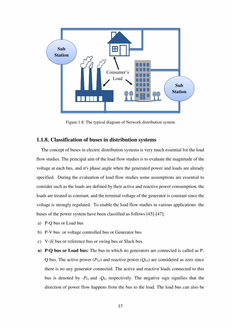
1.1.7. Network distribution system

Network distribution system is the system in which the feeder loop is

powered(energized) by two or more substations or generating stations. Network

distribution system is an interlocking loop system and is more complicated compared to

remaining systems. These systems used only in downtown regions, congested, and high

load municipal areas. The typical diagram of network distribution system is shown Fig.

1.8. Any area can be fed from two generating stations simultaneously during peak load

hours which causes the efficiency of the system to be increased and the reserve power

capacity of the network distribution system to be reduced.

Advantages of network distribution system:

1) This system is more reliable than radial and loop distribution systems since this system

comprised with two or more substations.

2) The efficiency of this system is high compared to radial and loop distribution systems.

Disadvantages of network distribution system:

1) This system is more expensive than radial and loop distribution systems.

2) This system is not simple in designing, planning, and operation.

17

Figure.1.8: The typical diagram of Network distribution system

1.1.8. Classification of buses in distribution systems

The concept of buses in electric distribution systems is very much essential for the load

flow studies. The principal aim of the load flow studies is to evaluate the magnitude of the

voltage at each bus, and it's phase angle when the generated power and loads are already

specified. During the evaluation of load flow studies some assumptions are essential to

consider such as the loads are defined by their active and reactive power consumption, the

loads are treated as constant, and the terminal voltage of the generator is constant since the

voltage is strongly regulated. To enable the load flow studies in various applications the

buses of the power system have been classified as follows [45]-[47]:

a) P-Q bus or Load bus

b) P-V bus or voltage controlled bus or Generator bus

c) V-|δ| bus or reference bus or swing bus or Slack bus

a) P-Q bus or Load bus: The bus in which no generators are connected is called as P-

Q bus. The active power (PGi) and reactive power (QGi) are considered as zero since

there is no any generator connected. The active and reactive loads connected to this

bus is denoted by -PLi and -QLi respectively. The negative sign signifies that the

direction of power flow happens from the bus to the load. The load bus can also be

Sub Station

Sub Station

Consumer’s Load

18

called as load bus. The principal aim of the load flow in this bus system is to evaluate

the magnitude of bus voltage |Vi| and its phase angle δi.

b) P-V bus or voltage controlled bus or Generator bus: The bus in which the

generators are connected is called as P-V bus. The power generation and terminal

voltage in P-V bus system are controlled by using prime mover and the generator

field excitation respectively. In these bus system the value of PGi and | Vi | can be

specified constant by keeping the bus voltage and input power constant using an

automatic voltage regulator and turbine governor control respectively. Hence, these

bus system is called as P-V bus. The p-v bus is also be called as voltage controlled

bus or generator bus. The reactive power(QGi) supplied by the generator can not be

specified in advance since it depends on the configuration of the system. The principal

aim of the load flow in this bus system is to find the unknown bus voltage phase

angle (δi).

c) V-|δ| bus or reference bus or swing bus or Slack bus: The bus, which sets the

reference angle for all remaining buses in the system, is known as V, |δ| bus. This bus

is also called as a slack bus or reference bus. This bus is the very essential for the load

flow studies without which load flow studies are meaningless. However, the angle of

the slack bus is not important for load flow studies since the active and reactive power

between two voltage sources can be dictated by the difference between the phase angle

of the two voltage sources. Hence, the angle of the slack bus is preferred as 0°. Also,

the voltage magnitude of the slack bus is assumed as prespecified value.

1.3. Research background on electrical distribution systems

Recent years the planning of distribution systems are prominently essential in power

system because of the wide variations in the strategies of the power supply [48], [49]. The

operation of electrical power distribution system is subjected to high power losses due to

high resistance to reactance ratio [50] as compared to high voltage transmission systems,

i.e. due to lower operating voltage and hence high current [51]. Also, suffers from line

loadability, poor voltage profile at the end nodes and poor voltage stability, etc. [52]-[56].

Since distribution systems are suffering from high power losses, it is a challenge to the

19

utilities to plan distribution systems to provide power for the cheapest possible rate and to

serve reliable and good quality of electrical power to the distributed consumers in the

present competitive environment [57]. Hence, it is important that the distribution

companies (DISCOs) should design RDNs properly to optimize their operation and the

energy loss, voltage profile, and voltage stability, etc. [58], [59]. Thus, the utilities are

adopting various advanced strategies to mitigate these problems by compensating the

reactive power in the distribution system.

The reactive power compensation schemes, such as capacitor bank placement [60], on

load tap changers [61], combinatorial operation of capacitor banks and on load tap changer

[62] and [63], incorporation of DG (distributed generation) [64] and [65], etc. can reduce

the power loss and improve the voltage profile and stability etc. Switched shunt capacitors

are optimally placed in a radial distribution system in a fuzzy multi-objective approach by

using a genetic algorithm (GA) to maximize the net savings and to minimize energy loss

and voltage drop [66]. Capacitor banks are optimally placed in the distribution systems to

reduce power loss in [67]. The optimal capacitor placement using particle swarm

optimization is reported in [68]. Cuckoo search optimization technique applied to capacitor

placement on distribution system problem [69]. However, capacitors are not capable of

providing smooth reactive power compensation and suffering from inevitable oscillations

along with the inductive elements in a system [70]. The optimally distributed generation

allocation and sizing in distribution systems via artificial bee colony algorithm has been

investigated in [71]. DGs are used for the DN to optimize the energy loss and benefit–cost

analysis of DG installation by optimally sizing and allocating it on DN [72] - [75].

However, DG sources are relatively high costs, and intermittency [76] - [79].

Nowadays, DFACTS (distribution FACTS) devices such as Unified Power Quality

Conditioner (UPQU), static VAR compensators (SVC), Distribution static synchronous

series compensator (DSSSC) and distribution static synchronous compensator

(DSTATCOM) etc. [56] and [122] are used for the reactive power compensation, because

of the rapid advancement of power electronic devices. A comprehensive review has been

done on optimization techniques for the placement and sizing of custom power devices in

RDNs [80]. UPQC is used to compensate the reactive power in radial distribution systems

20

[81], and the impact of its online allocation loading, losses, and voltage stability is

investigated in [82]. A multi-objective planning strategy for UPQC allocation by

minimizing three objective functions, such as the rating of UPQC, system power loss, and

percentage of nodes with under voltage problem is provided in [83] to determine its

optimal location(s) and size(s). A state-of-art review on the different reactive power

compensation techniques including the allocation strategies of custom power devices, such

as SVC is reported in [84]. DSSSC (distribution static synchronous series compensator) is

used to reduce the power loss and to enhance the voltage profile in RDNs [85]. Some of

the power quality issues of electrical distribution systems influenced by the allocation of

DSTATCOM with distribution generator are given in [86]. These devices are optimally

sized and allocated in the radial distribution system by using a particle swarm optimization

algorithm to compensate the reactive power for the reduction of power loss [87]. The

optimal allocation of DSTATCOM along with network reconfiguration by using

differential evolution algorithm is carried to minimize the power loss of radial distribution

systems in [57]. Modeling and optimal allocation for DSTATCOM for the compensation

of reactive power in radial distribution systems are presented in [88]. The reactive power

is compensated by using DSTATCOM for distribution systems with wind energy in [89].

By using the combination of both DVR & DSTATCOM, the voltage sag is mitigated with

and without injection of real and apparent power in RDN when faults are occurred [90].

The combination of optimal operation and network reconfiguration of the distribution

system is a complicated problem [92] since the network reconfiguration results in a change

in topology of feeder structure by opening or closing of sectionalizers. Moreover, the

control of DSTATCOM with DG in the distribution systems is complex, and a DVR is

costlier as compared to a DSTATCOM [57]. However, the installation and maintenance

costs of combinatorial schemes are high and complexity in operation [91].

Among all these devices discussed above DSTATCOM has several advantages such as

reduces the system power loss with reactive power exchange, high regulatory capability,

low compact size and low cost and less harmonic production and does not have any

transient harmonic operational problems. Also, DSTATCOM mitigates the power quality

problems such as voltage fluctuations, voltage sag, unbalanced load, and voltage

21

unbalance and. [123] and [124]. A distribution static compensator (DSTATCOM) is a

power electronic based synchronous VSC (voltage source converter) that generates an AC

voltage by a short-term energy stored in a DC capacitor. The reactive power exchange

between the device and the distribution system can be controlled by controlling the

magnitude of the voltage at D-STATCOM [125] and [126].

Hence, In view of all these problems, it is interesting to investigate the impact of

optimal allocation of single and multiple DSTATCOM in RDS to optimize voltage profile,

power loss, total planning cost of energy loss per annum or energy loss cost (ELC).

Modeling, sizing, and allocation of single DSTATCOM on radial distribution systems to

optimize the power loss and improve the voltage profile by compensating the reactive

power are investigated in [56], [68], [70], [73], and [93]-[96].

1.4. Motivation

There are several factors that encouraged deciding this topic for the thesis. Still, the

primary sources of motivation for this work are:

1. Distribution systems are traditionally suffering from high power loss compared to

transmission systems, poor voltage profile. These problems are causing the poor

power quality in the supply of power to the consumers.

2. Most of the previous investigations introduced the allocation of capacitors and

combinatorial devices to compensate the reactive power in RDS to reduce power

loss and improve voltage profile. But, capacitors are incapable of providing smooth

reactive power compensation and suffering from inevitable oscillations along with

the inductive elements in a system.

3. Combinatorial devices as mentioned in section 1.2 used for the reactive power

compensation in radial distribution systems to minimize power loss are not

economical and increases the complexity of control and operation of the device

and system.

4. Very few investigations have been contributed in recent days to optimize the

energy loss cost of RDS per annum and PH with the optimal allocation of

appropriate DSTATCOM model.

22

5. New work on Multiple DSTATCOM required to be investigated since the distinct

combinatorial devices are not economical and increase the complexity of control

and operation.

In view of all these problems, it is interesting to investigate the impact of optimal

allocation of single and multiple DSTATCOM on RDS to optimize the voltage profile,

power loss, the energy loss cost, total net profit or economic benefit per annum and PH.

1.5. Objectives of thesis

1. Devising a new modeling of DSTATCOM to incorporate it in RDS.

2. Developing FBS load flow algorithm and incorporation of DSTATOM in FBS

algorithm.

3. Formulation of the objective function to evaluate the objectives of proposed

approach such as the power loss, voltage profile, energy loss cost, total net profit

per annum and PH.

4. Development of ESM algorithm to find the optimal allocation and rating of

DSTATCOM in radial distribution systems to optimize the power loss, voltage

profile, energy loss cost, total net profit per annum and PH.

5. Development of DEA algorithm to find the optimal allocation and rating of

DSTATCOM in radial distribution systems to optimize the power loss, voltage

profile, energy loss cost, total net profit per annum and PH.

1.6. Work done

In this Thesis, a new phase angle model for DSTATCOM based on optimal angle

injection (DSTATCOM-OAI) is developed. In the proposed model, the rating of the

DSTATCOM is determined with the injection of the optimal phase angle of the voltage

phasor at the location, in which a DSTATCOM is placed. The DSTATCOM model is

suitably incorporated into the FBS load flow algorithm [97] to minimize total active power

loss. Exhaustive search and Differential Evolution (DE) algorithm [98] - [101] is used to

determine the optimal locations and sizes for DSTATCOM, ELC, and total net profit

(TNP) in RDS. The IEEE-30, 33 and 69 node radial distribution system are used as test

systems o demonstrate the proposed approach, and it is noteworthy that there is a

23

significant reduction in power loss and ELC and improvement of voltage profile and TNP

after the placement of DSTATCOM on the radial distribution system. The results of the

proposed approach are found to be better as compared to approaches reported in [51], [31],

[87], [88], [102], and [103].

1.7. Thesis organization

The entire thesis is divided into seven chapters. The organization of the thesis and a

brief chapter wise description of the work presented are as follows:

Chapter 1 provides the overview of electrical distribution systems and their classifications

with merits and demerits. The different power quality issues occurring in electrical

distributions systems are discussed. The previous investigations upon solving some of the

power quality issues are discussed. Why the need for research in electrical distribution

systems has been studied based on previous research background. This chapter provides

the strong reasons that what motivates the author to opt the proposed approach. The

objectives and contributions of the proposed approach are mentioned in this chapter.

Chapter 2 discussed the development of new phase angle model of DSTATCOM and its

incorporation in FBS algorithm. The FBS algorithm and flow chart developed are provided

in this chapter. Also, the principle of operation of DSTATCOM is described.

Chapter 3 proposes the distribution STATCOM with optimal phase angle injection model

for reactive power compensation of radial distribution systems using DEA and ESm

techiniques. Firstly, the brief disruption on ESM and is algorithm in proposed approach

are described. Secondly, Overview and flow chart of DEA and the optimal allocation of

DSTATCOM using DEA are provided in this chapter. The solution strategy of DEA and

the comparative simulation results and exhaustive search results are discussed in this

chapter.

Chapter 4 deals with the optimization of energy loss cost of distribution systems with the

optimal placement and sizing of DSTATCOM using differential evolution algorithm.

mathematical problem formulation i.e. objective function (F), real power loss, present

worth factor (PWF) analysis, TNP/Savings, constraints, solution strategy using DEA,

24

simulation results, impact of DSTATCOM allocation, analysis of power loss reduction,

analysis of ELC are discussed.

Chapter 5 investigates optimal phase angle injection for reactive power compensation of

distribution systems with the allocation of multiple distribution STATCOM and the

combination of DSTATCOM and DG. Why for multiple DSTATCOM allocations, results

of multiple-DSTATCOM allocation using DE, Comparative results with some of the

previous works, and the solution obtained with proposed de algorithm, in 50 runs for the

69-node system are discussed.

Chapter 6 concludes the thesis by summarizing the contributions and conclusions of all

the chapters. Ultimately, the final section explores future directions of research that

emerged as an outcome of the work presented in this thesis.

25

Chapter 2

Phase angle model of DSTATCOM and its Incorporation in FBS algorithm

2.1. Introduction

This chapter presents the principle of operation of DSTATCOM and the new phase

angle model of DSTATCOM devised and its incorporation in FBS algorithm to investigate

the impact of its placement on power loss reduction, cost of energy loss and voltage profile.

In a distribution system, there may be several different compensating devices.

However, in a radial distribution system, the voltage profile of a particular bus can be poor

or distorted or unbalanced if the demand is increased suddenly or loads in any part of the

system are nonlinear or unbalanced. The power quality problems in the DS usually

originate from voltage disturbances and power loss. In DS the maximum amount of power

gets consumed by the reactive loads, as a result there is increase in lagging power factor

current drawn by these loads. Hence, the demand of excessive reactive power increases,

which causes the reduction in the capability of active power flow, increase in power loss

and poor voltage profile. Therefore, in recent days the voltage profile and power loss

predominantly play vital role in the planning and operation of DS. Thus, the main reason

of poor voltage profile and power loss in DS is the excessive demand of reactive power

and increase in load. The DSTATCOM, which belongs to the family of DFACTS devices

can compensates the reactive power statically in the DS to minimize the power loss and

improve the voltage profile.

Before entering into the discussion of the new phase angle model of DSTATCOM and

its incorporation in load flow algorithm for achieving the objectives of the proposed

approach, it is very much essential to know what is the operation of FBS load flow

algorithm, and why and how it’s used in the proposed approach and what is DSTATCOM,

what are the components used in the design of DSTATCOM, how the working principle

of DSTACOM involved in proposed approach.

26

2.2. DSTATCOM in the proposed approach

2.2.1. What is DSTATCOM?

DSTATCOM is a fast response solid-state power electronic based shunt controlled

voltage source converter (VSC) which injects the current to the utility feeder or nodes in

distribution systems for the smooth reactive power compensation to improve the power

quality in DS such as enhancement of the voltage profile and minimization of the power

loss of the DS [104]-[106]. Mainly it consists of an inverter, which works on the principle

of self-commutation control. The output voltage of the DSTATCOM can be controlled

according to the requirement of the reactive power since it is a voltage-sourced converter.

The DSTATCOM can be called in other words that it is a distribution static synchronous

condenser (DSTATCON). Usually, this device is sustained by a DC energy storage

capacitor. It generates the inductive and capacitive reactive power according to the load

demand to meet the specifications of utility[104].

2.2.2. Components involved in DSTATCOM design

The DSTATCOM consists of an IGBT based VSC (voltage source converter), DC

storage capacitor and a coupling transformer as shown in Fig. 2.2

1) Voltage Source Converter(VSC):

VSC is used to convert the DC input voltage to an AC output voltage at fundamental

frequency and generates or absorbs the reactive power.

2) DC storage capacitor or energy storage device:

DC storage is used to supply constant DC voltage to the voltage source converter

(VSC) via a DC link capacitor for the generation of injected voltages.

3) Coupling transformer:

A coupling transformer is one, which couples two different voltage signals. It couples

the output voltage of VSC and bus voltage of DS voltage through the reactance. In

addition, the inductive reactance of transformer minimizes ripples contained in the

compensating currents produced by VSC. The inductive reactance of transformer can

also be called as interfacing reactance. Coupling transformer used at AC side of VSC

as shown in Fig. 2.2. The coupling transformer can also provide isolation between the

27

inverters of multilevel inverter structure, which avoids the DC storage capacitor from

being short-circuited with the inverters through switches.

2.2.3. Working principle of DSTATCOM

In this section, the working principle of DSTATCOM according to its application in

the approach proposed in thesis is elaborately discussed. In the proposed approach,

DSTATCOM is used for reactive power compensation in DS to reduce power loss and

improve voltage profile.

The Basic Arrangement of DSTATCOM is as shown in Fig.2.2. The reactive power

exchange between the DSTATCOM and DS can be regulated by varying the output

voltage of DSTATCOM (VSC), so that the DS voltage profile be improved. DSTATCOM

in general is an IGBT based VSC. The principle of operation of DSTATCOM is same as

to the operation of a rotating synchronous electrical machine without the mechanical

inertia, which either absorbs or generates the reactive power in synchronization according

to the demand. Hence, DSTATCOM is called as a distribution static synchronous

compensator.

Figure.2.1: A simple line diagram of an electric line connected between two consecutive voltage

sources

First of all the phenomenon of the reactive power transfer equation is described before

the principle of operation of DSTATCOM is discussed so that it would be understood very

easily. As shown in Fig. 2.1 two voltage sources VS and VR that are connected each other

through an impedance Z = R + jX, and the current flowing through the impedance branch

is Ib are considered. The resistance R is assumed to be as zero and the difference of angle

between VS and VR is ‘δ’ expressed by Eq. (2.1).

S R (2.1)

28

The active power flow exists between the two voltage as shown in Fig.2.1 is expressed by

Eq. (2.2)

S RV VP Sin

X (2.2)

Similarly, the reactive power flow exists between the two voltage is given in Eq. (2.3)

RS R

VQ V Cos V

X (2.3)

If the ‘δ’ is ‘zero’ then the active and reactive, power becomes as given Eqs. (2.4) and

(2.5) respectively:

0P (2.4)

RS R

VQ V V

X (2.5)

From Eqs (2.4) and (2.5) it is very clear that if the difference of angle between VS and VR

is zero, the active power (P) flow becomes zero and the reactive power (Q) flow depends

on ‘VS -VR’. Hence, the reactive power flow in the system happens in two ways. Firstly, if

the voltage VS is greater than VR, then the reactive power flow happens from the source VS

to VR. Secondly, if VR is greater than VS, then reactive power flow happens from the source

VR to VS. This same principle is applied in the working principle of DSTATCOM.

Now it is very easy to understand how the working principle of DSTATCOM. A typical

RDS, as shown in Fig. 2.2. is considered for the implementation of DSTATCOM

operation. It consists of ‘n’ number of buses connected to a stiff voltage source at bus ‘V1’.

There is a load connected at each bus and are supplied by respective buses. Based on the

reactive power need of utility or particular customer the DSTATCOM is subjected to be

connected in any bus. E.g. if the voltage ‘V3 (BUS)’ is disturbed, all buses except slack bus

will be affected, and then the utility installs a DSTATCOM at ‘bus 3’ to mitigate the

voltage problem. If the same happens with consumers load then the consumer installs the

DSTATCOM in the premises of the problem occurred.

Let ‘V3 (BUS)’ be the bus voltage of DS and ‘VDSTATCOM’ be the output voltage of the

DSTATCOM as shown in Fig. 2.2. The reactive power flows only when the angle between

two voltages is zero i.e. ‘VDSTATCOM’ is in phase with ‘V3 (BUS)’ during steady state condition.

29

The reactive power exchange is zero if the magnitude of ‘V3 (BUS)’ is equal to ‘VDSTATCOM’,

as a result the DSTATCOM neither generate nor absorb the reactive power. The flow of

reactive power is discussed in two modes of operations, which is also called as voltage

regulation mode such as:

Figure.2.2: A simple Radial distribution line with the allocation of DSTATCOM

1) Inductive mode or Q-generation

2) Capacitive mode or Q-absorption.

1) Inductive mode or Q-absorption

If the magnitude ‘VDSTATCOM’ is less than ‘V3 (BUS)’, the DSTATCOM, feels the

capacitive reactance connected at its output terminals, simultaneously the DS feels the

inductive reactance at the PCC where the DSTATCOM is connected. Hence, the

S2-load S3-load Sn-load S1-load

V1 V2 V3 Vn

VS

IS

IDSTATCOM

Coupling Transformer

DC Storage

VSC

DSTATCOM

VDSTATCOM

30

DSTATCOM current ‘IDSTATCOM’ lags behind the voltage of DS exactly by an angle of

90º as shown in Fig.2.3 and allows the DS currents to flow into it, which causes the

DSTATCOM to absorb reactive power. That is how, the reactive power flows from

DS to DSTATCOM through the coupling transformer. Thus, the DSTATCOM absorbs

the reactive power. Generally, this mode occurs when the bus voltage of DS increased

due to load throw off or some other abnormal situations. At this situation,

DSTATCOM reduces ‘VDSTATCOM’ and therefore absorbs the reactive power so that the

voltage reaches to its normal value. The time diagram of the DSTATCOM voltage and

current during this mode of operation is shown in Fig.2.3

Figure.2.3: The time diagram of DSTATCOM voltage and current in inductive mode of operation (absorption of Q)

2) Capacitive mode or Q-generation

If ‘VDSTATCOM’ is greater than ‘V3 (BUS)’ the DSTATCOM, feels the inductive reactance

connected at its output terminals, simultaneously the DS feels the capacitive reactance

at the PCC where the DSTATCOM is connected. Hence, the DSTATCOM current

‘IDSTATCOM’ leads the voltage of DS exactly by an angle of 90º as shown in Fig.2.4 and

gets injected into the DS which causes the DSTATCOM to generate reactive power.

That is how, the reactive power flows from DSTATCOM to DS through the coupling

transformer. Thus, the DSTATCOM behaves like as reactive power (Q) generator.

Usually, this mode occurs when the reactive power demand increased in the DS. At

this situation, DSTATCOM increases its output voltage ‘VDSTATCOM’. The time diagram

IDSTATCOM V3 (BUS) VDSTATCOM

Phase angle

V or I

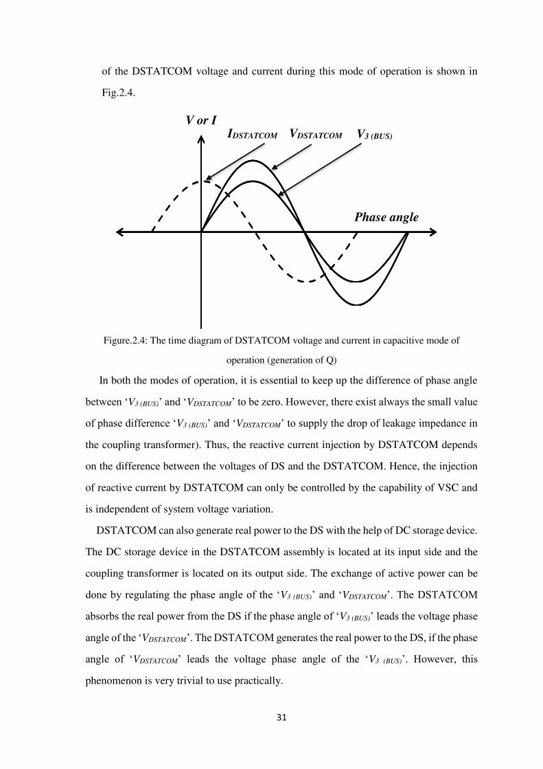
31

of the DSTATCOM voltage and current during this mode of operation is shown in

Fig.2.4.

Figure.2.4: The time diagram of DSTATCOM voltage and current in capacitive mode of

operation (generation of Q)

In both the modes of operation, it is essential to keep up the difference of phase angle

between ‘V3 (BUS)’ and ‘VDSTATCOM’ to be zero. However, there exist always the small value

of phase difference ‘V3 (BUS)’ and ‘VDSTATCOM’ to supply the drop of leakage impedance in

the coupling transformer). Thus, the reactive current injection by DSTATCOM depends

on the difference between the voltages of DS and the DSTATCOM. Hence, the injection

of reactive current by DSTATCOM can only be controlled by the capability of VSC and

is independent of system voltage variation.

DSTATCOM can also generate real power to the DS with the help of DC storage device.

The DC storage device in the DSTATCOM assembly is located at its input side and the

coupling transformer is located on its output side. The exchange of active power can be

done by regulating the phase angle of the ‘V3 (BUS)’ and ‘VDSTATCOM’. The DSTATCOM

absorbs the real power from the DS if the phase angle of ‘V3 (BUS)’ leads the voltage phase

angle of the ‘VDSTATCOM’. The DSTATCOM generates the real power to the DS, if the phase

angle of ‘VDSTATCOM’ leads the voltage phase angle of the ‘V3 (BUS)’. However, this

phenomenon is very trivial to use practically.

VDSTATCOM V3 (BUS) IDSTATCOM

Phase angle

V or I

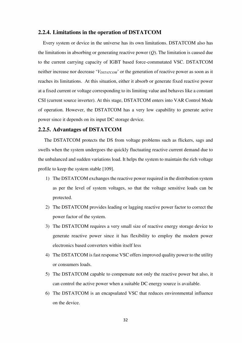
32

2.2.4. Limitations in the operation of DSTATCOM

Every system or device in the universe has its own limitations. DSTATCOM also has

the limitations in absorbing or generating reactive power (Q). The limitation is caused due

to the current carrying capacity of IGBT based force-commutated VSC. DSTATCOM

neither increase nor decrease ‘VDSTATCOM’ or the generation of reactive power as soon as it

reaches its limitations. At this situation, either it absorb or generate fixed reactive power

at a fixed current or voltage corresponding to its limiting value and behaves like a constant

CSI (current source inverter). At this stage, DSTATCOM enters into VAR Control Mode

of operation. However, the DSTATCOM has a very low capability to generate active

power since it depends on its input DC storage device.

2.2.5. Advantages of DSTATCOM

The DSTATCOM protects the DS from voltage problems such as flickers, sags and

swells when the system undergoes the quickly fluctuating reactive current demand due to

the unbalanced and sudden variations load. It helps the system to maintain the rich voltage

profile to keep the system stable [109].

1) The DSTATCOM exchanges the reactive power required in the distribution system

as per the level of system voltages, so that the voltage sensitive loads can be

protected.

2) The DSTATCOM provides leading or lagging reactive power factor to correct the

power factor of the system.

3) The DSTATCOM requires a very small size of reactive energy storage device to

generate reactive power since it has flexibility to employ the modern power

electronics based converters within itself less

4) The DSTATCOM is fast response VSC offers improved quality power to the utility

or consumers loads.

5) The DSTATCOM capable to compensate not only the reactive power but also, it

can control the active power when a suitable DC energy source is available.

6) The DSTATCOM is an encapsulated VSC that reduces environmental influence

on the device.

33

2.3. The new phase angle Model of DSTATOCM

As discussed above the DSTATCOM is a shunt connected VSC device that absorbs or

injects both active and reactive current respectively through PCC [70]. In the proposed

approach, DSTATCOM is used only for reactive power compensation in DN to improve

the voltage profile and minimize the power loss and coast of energy loss cost.

Figure.2.5: Two successive buses of DN drawn as a single line diagram

Figure.2.6: Phasor diagram for the network shown in Fig.2.5

Fig. 2.5. is the single line diagram of two successive buses n and n+1 of DN and there

are real and reactive power demands connected to these buses, and it is used to place the

DSTATCOM in DN. The Kirchhoff’s voltage law equation of the Fig.2.5. is given by

Eq.(2.6).

Ib

P jQn n

1 1P jQn n

Rb

jXb

nV 1nV

Vn

jX Ib b

1V

n

R Ib b

Ib

Reference axis

1n

n

34

1 1V V R jX Ibn nn n b b (2.6)

In above Eq. (2.6), Rb+jXb is the line impedance between two nodes, Vn is the voltage at

the nth node, αn is the phase angle of Vn, Ib is the line current between the two nodes n and

n+1, and θ is the phase angle of Ib. Pn and Qn are the active and reactive power loads at

node n. Fig. 2 is the phasor representation of the Eq. (2.6).

Figure.2.7: Single line diagram with a DSTATCOM placed at bus n+1

To develop the phase angle model of DSTATCOM, it is allocated at node n+1 as shown

in Fig. 2.7. The KVL of single line diagram after the placement of DSTATCOM is

expressed in Eq. (2.7).

' '' ' '1 1 12

V V R jX I Ibn n DSTATn n b b n

(2.7)

The phasor diagram corresponding to the Eq. (2.7) is shown in Fig. 2.8. With the allocation

of DSTATCOM at node n+1 through PCC, the voltage at node n+1 is reformed as V 'n+1

due to the injection of phase angle. The Eq. (2.7) is the main essence for developing the

phase angle model of DSTATCOM. The angle of the IDSTAT is expressed as follows

'12

I DSTAT n (2.8)

PCC

Ib

P jQn n

1 1P jQn n

IDSTAT

DSTATCOM

Rb

jXb

( )VSC

Energy Storage

'1nV

'nV

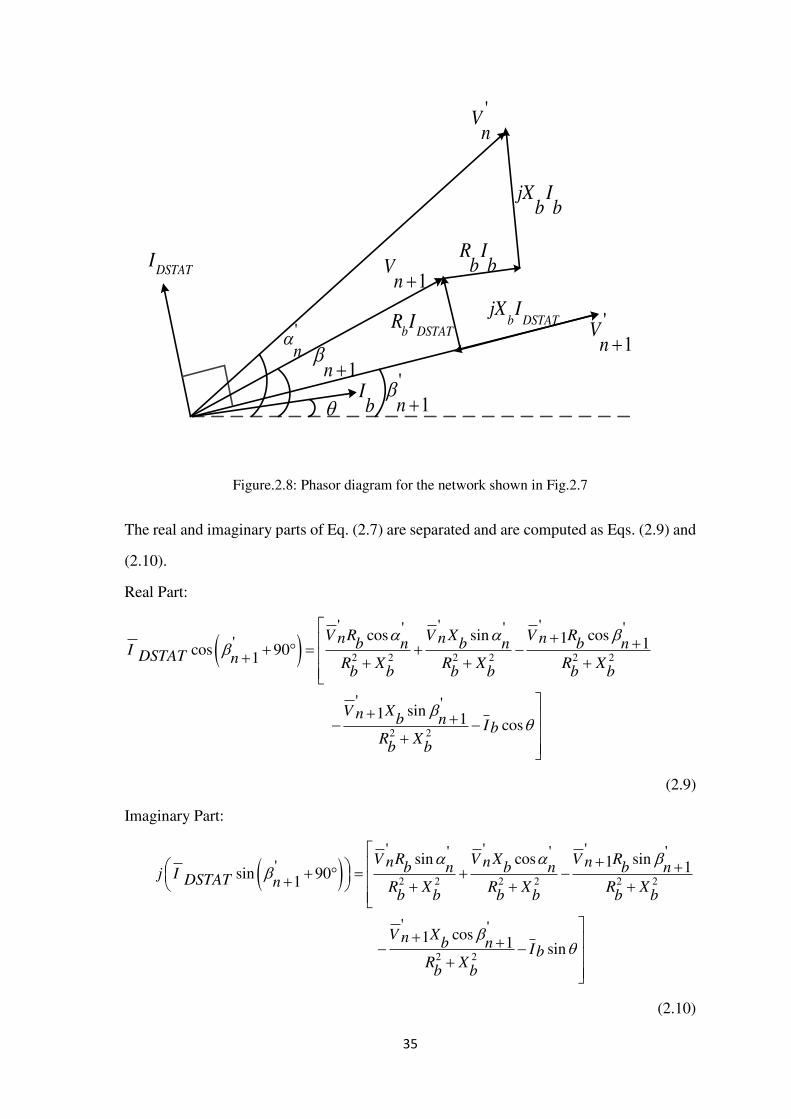
35

The real and imaginary parts of Eq. (2.7) are separated and are computed as Eqs. (2.9) and

(2.10).

Real Part:

2 2 2 2 2 2

2 2

' ' '' ' 'cos sin cos1' 1cos 901

' 'sin1 1 cos

V R V X V Rn n nb n b n b nI DSTAT n R X R X R Xb b b b b b

V Xn b n IbR Xb b

(2.9)

Imaginary Part:

2 2 2 2 2 2

2 2

' ' '' ' 'sin cos sin1' 1sin 901

' 'cos1 1 sin

V R V X V Rn n nb n b n b nj I DSTAT n R X R X R Xb b b b b b

V Xn b n IbR Xb b

(2.10)

Figure.2.8: Phasor diagram for the network shown in Fig.2.7

'Vn

Reference axisReference axis

'1

Vn

DSTATI R Ib b

jX Ib b

1V

n

1n

'1n

b DSTATR I b DSTATjX I

'n

Ib

36

Let,

2 2 2 2 2 2 2 2

' ' ' '1 1

, , , , ,

' 90 ,1

V R V X V R V Xn n n nb b b ba b c d e I DSTATR X R X R X R Xb b b b b b b b

and Ibn

By replacing these parameters in Eqs. (2.9) and (2.10), the magnitude of the injected

current of DSTATCOM has obtained as:

1 2'sin

sin

K K nI DSTAT

(2.11)

Where, , ,

“φ” is a unique angle satisfying the following conditions:

Finally, Eq. (2.11) is the current which must be injected at a required n+1th bus of DN to

compensate the reactive power to reduce the power loss. Hence the reactive power that

can be provided by the DSTATCOM is expressed as follows:

(2.12)

The symbol ‘*’ in Eq. (2.12) designates the complex conjugate. Eq. (2.12) is integrated

into the load flow algorithm through the DEA to compute the load flow parameters voltage

magnitude of each bus and the total power loss of the network. There are certain variables

K1, K2, α'n, β'

n+1, θ, φ, and ψ In Eq. (2.11). These variables decide IDSTAT, and the value of

IDSTAT gets varied if the location of DSTATCOM is changed. Since the phase angle (β'i+1)

injection by DSTATCOM in node n+1 of RDS impacts the power loss to be reduced

optimally, the phase angle (β'i+1) injected in that node has been considered as an optimal

variable. All the variables, except the optimal variable phase angle ‘β'i+1’ are evaluated by

the forward-backward sweep (FBS) load flow algorithm provided in next section.

1' 'sin cos1 1K a bn n

2 22

'

2 2V nK c d

R Xb b

) ,

) , 0, 0

i

Xd bii tan Since d cc Rb

'.1DSTAT DSTATjQ V In

37

However, for the very first iteration of the operation of FBS load flow algorithm, initially,

a constant voltage of all nodes is assumed to be l p.u.∠0. The phase angle ‘β'i+1’ selected

by DE algorithm is injected into the reactive power load of the bus data of RDS in each

iteration of the FBS load flow algorithm [99].

2.4. Incorporation of phase angle model of DSTATCOM in

FBS algorithm

In the proposed approach, the best location and size of the DSTATCOM in RDS at

different load levels have been found using the differential evolution optimization

technique when the FBS algorithm is integrated in DEA. The DEA is worthless in the

proposed approach without FBS algorithm. Line currents, bus voltages and power loss of

RDS in each generation of DEA have been evaluated by FBS algorithm only when the size

of the DSTATCOM is incorporated in FBS load flow algorithm through the data of RDS.

Before discussing how the new phase angle model of DSTATCOM is incorporated in FBS

load flow algorithm in the proposed approach, it is necessary to discuss how the FBS load

flow technique works.

2.4.1. FBS Load flow technique

The proposed FBS load flow technique works based on to stages of evaluation, first

stage is backward sweep and second stage is forward sweep. In first stage, all load and line

currents are calculated and in second stage, all node voltages are determined using the

results of first stage, these two stages depend on each other to perform the load flow

calculations. Before these stages are started, initially each node voltage is assumed to be

constant l p.u.∠0º. At the end of second stage, convergence condition is checked. If the

convergence condition is not satisfied, then again first stage calculations are done using

the most recent results of second stage, and this process reappears till the convergence

condition is satisfied. The convergence condition is set as the value 1X10-3 p.u. is greater

than the maximum voltage magnitude difference in the successive iterations. This

operation of FBS load flow technique in RDS is discussed below.

First of all, a simple RDS has been considered as shown in Fig. 2.9 for the application

of FBS load flow technique. As it can be seen in Fig. 2.9 that all node voltages are assumed

38

as l p.u.∠0º. The loads at each node are represented by S1-load S2-load S3-load and S4-load

respectively, and I12, I23, and I34 are the line currents and I1, I2, and I3 are the load currents

and IS is the source current and Z12, Z23, and Z34 are the line impedances of the RDS.

Figure.2.9: Simple RDS considered for FBS load flow studies

a) Backward Sweep operation

As discussed above in this operation the line currents of RDS are evaluated. Initially,

the load current are calculated as shown in below Eqs. (2.13) to (2.16).

* *1 1 1 1 1

11 1 1 0

S P jQ P jQI

V V

(2.13)

* *2 2 2 2 2

22 2 1 0

S P jQ P jQI

V V

(2.14)

* *

3 3 3 3 33

3 3 1 0S P jQ P jQ

IV V

(2.15)

* *4 4 4 4 4

44 4 1 0

S P jQ P jQI

V V

(2.16)

In above equations each value of active and reactive loads are taken from the data of RDS.

Since this operation speaks about backward sweep, the line currents are calculated in

backward direction from last bus using KCL applied at the buses 4, 3, and 2 and are

expressed as given in Eqs. (2.17) to (2.20).

34 4I I (2.17)

S2-load S3-load S4-load S1-load

IS

VS = 1 0º

I34 I23 I12

V1 = 1 0º V2 = 1 0º V3 = 1 0º V4 = 1 0º

I1 I2 I3 I4

Z12 Z34 Z23

39

23 34 3I I I (2.18)

12 23 2I I I (2.19)

12 1SI I I (2.20)

b) Backward Sweep operation

In this operation, the all bus voltages except the substation bus voltage ‘V1’of RDS are

evaluated since the substation bus is referred as slack bus as discussed in ‘section 1.1.8’ of

‘chapter 1’. Since this operation speaks about forward sweep the voltages are evaluated in

forward direction from ‘bus 2’ using the equations expressed in Eqs. (2.21) to (2.23).

2 1 12 12V V I Z (2.21)

3 2 23 23V V I Z (2.22)

4 3 34 34V V I Z (2.23)

c) Convergence criteria

The convergence criteria is one which checks the accuracy of the values obtained in the

operation of FBS load flow technique and checks it with the prespecified value set for the

convergence condition. If the condition is satisfied, it stops the operation and display the

results. To check the convergence the reference value of accuracy is set to a prespecified

value 0.0001 p.u. in proposed approach. The evaluation of accuracy involves with the

difference between the previous and present bus voltage obtained in iterative operations

as shown below Eqs. (2.24) to (2.26).

2 2 2old newV V V (2.24)

3 3 3old newV V V (2.25)

4 4 4old newV V V (2.26)

If the ΔV2 or ΔV3 or ΔV4 ≤ 0001 then the FBS load flow gets stopped, or else the operations

shall be repeated toll the convergence condition is satisfied.

Note: The load flow calculations are under per unit values.

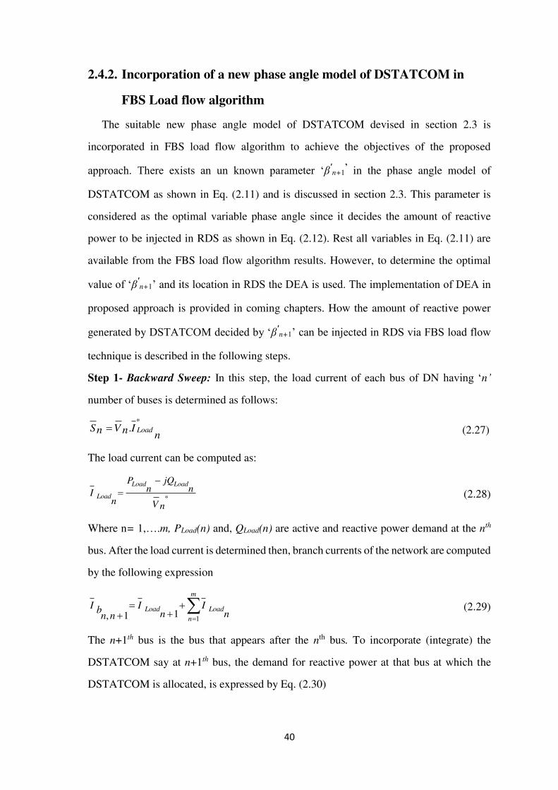
40

2.4.2. Incorporation of a new phase angle model of DSTATCOM in

FBS Load flow algorithm

The suitable new phase angle model of DSTATCOM devised in section 2.3 is

incorporated in FBS load flow algorithm to achieve the objectives of the proposed

approach. There exists an un known parameter ‘β'n+1

’ in the phase angle model of

DSTATCOM as shown in Eq. (2.11) and is discussed in section 2.3. This parameter is

considered as the optimal variable phase angle since it decides the amount of reactive

power to be injected in RDS as shown in Eq. (2.12). Rest all variables in Eq. (2.11) are

available from the FBS load flow algorithm results. However, to determine the optimal

value of ‘β'n+1’ and its location in RDS the DEA is used. The implementation of DEA in

proposed approach is provided in coming chapters. How the amount of reactive power

generated by DSTATCOM decided by ‘β'n+1’ can be injected in RDS via FBS load flow

technique is described in the following steps.

Step 1- Backward Sweep: In this step, the load current of each bus of DN having ‘n’

number of buses is determined as follows:

(2.27)

The load current can be computed as:

(2.28)

Where n= 1,….m, PLoad(n) and, QLoad(n) are active and reactive power demand at the nth

bus. After the load current is determined then, branch currents of the network are computed

by the following expression

(2.29)

The n+1th bus is the bus that appears after the nth bus. To incorporate (integrate) the

DSTATCOM say at n+1th bus, the demand for reactive power at that bus at which the

DSTATCOM is allocated, is expressed by Eq. (2.30)

*. LoadS V In n n

*

Load Load

Load

P jQn nI

n V n

11, 1

m

Load Loadn

I I Ib n nn n

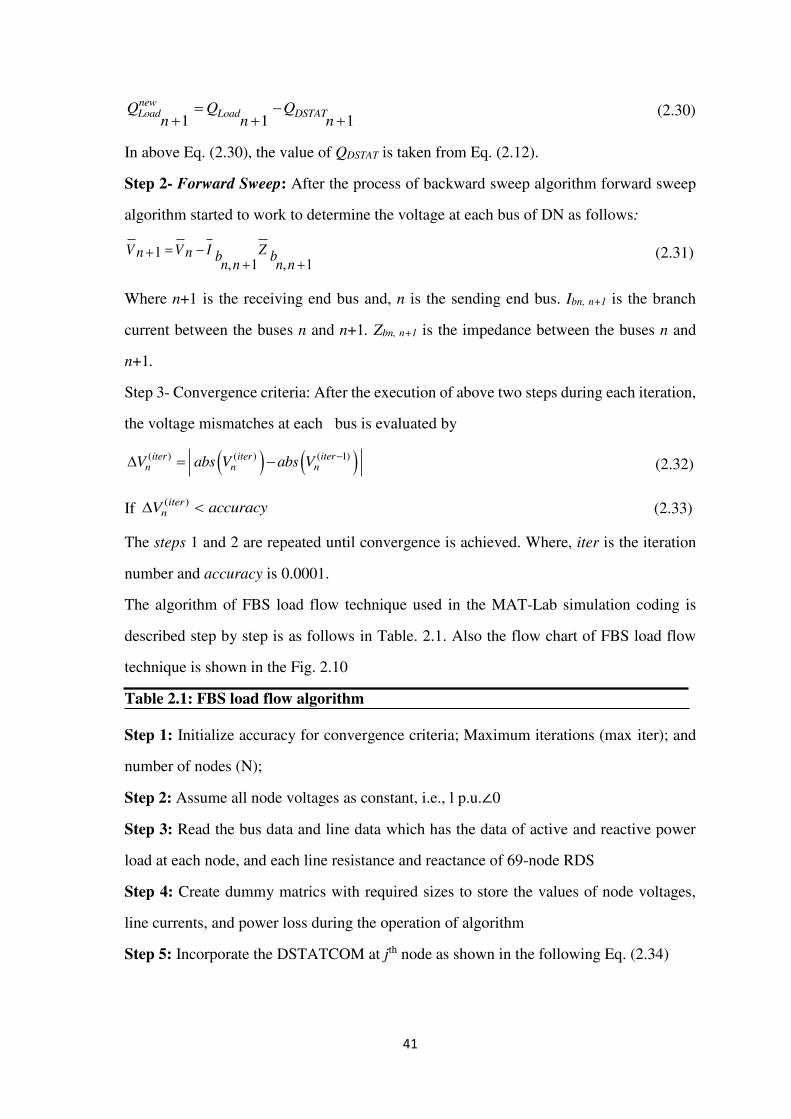
41

(2.30)

In above Eq. (2.30), the value of QDSTAT is taken from Eq. (2.12).

Step 2- Forward Sweep: After the process of backward sweep algorithm forward sweep

algorithm started to work to determine the voltage at each bus of DN as follows:

(2.31)

Where n+1 is the receiving end bus and, n is the sending end bus. Ibn, n+1 is the branch

current between the buses n and n+1. Zbn, n+1 is the impedance between the buses n and

n+1.

Step 3- Convergence criteria: After the execution of above two steps during each iteration,

the voltage mismatches at each bus is evaluated by

(2.32)

If (2.33)

The steps 1 and 2 are repeated until convergence is achieved. Where, iter is the iteration

number and accuracy is 0.0001.

The algorithm of FBS load flow technique used in the MAT-Lab simulation coding is

described step by step is as follows in Table. 2.1. Also the flow chart of FBS load flow

technique is shown in the Fig. 2.10

Table 2.1: FBS load flow algorithm

Step 1: Initialize accuracy for convergence criteria; Maximum iterations (max iter); and

number of nodes (N);

Step 2: Assume all node voltages as constant, i.e., l p.u.∠0

Step 3: Read the bus data and line data which has the data of active and reactive power

load at each node, and each line resistance and reactance of 69-node RDS

Step 4: Create dummy matrics with required sizes to store the values of node voltages,

line currents, and power loss during the operation of algorithm

Step 5: Incorporate the DSTATCOM at jth node as shown in the following Eq. (2.34)

1 1 1newLoad Load DSTATQ Q Q

n n n

1, 1 , 1

V V I Zn n b bn n n n

( ) ( ) ( 1)iter iter itern n nV abs V abs V

( )iternV accuracy

42

Reactive power load Reactive power load

Reactive power load

newj j

DSTATCOMj

(2.34)

Where, Reactive power loadDSTATCOMj = DSTATCOMjQ which is given in Eq. (2.12).

Step 6: Perform the operation of backward sweep to evaluate the line currents with the

help of following Eqs. (2.35), (2.36), and (2.37)

*Apparent power load Voltage Load currentnewj jj (2.35)

Active power load Reactive power loadLoad current

*Voltage

jj jj

j

(2.36)

Line current Load current Load current1

N

ij i ji

(2.37)

Step 7: Perform the operation of forward sweep to evaluate the node voltages using the

following Eq. (2.38).

Voltage Voltage Line current Line Impedancej i ij ij (2.38)

Step 8: Check the convergence criteria using the following Eqs. (2.39) and (2.40)

( ) ( ) ( 1)Voltage Voltage Voltagek k kabs absi i i

(2.39)

If ( )Voltage k accuracyi (2.40)

Step 9: Evaluate power loss (according to the power loss formulation in next chapter)

Step 10: If convergence criteria are not satisfied repeat from Step 5 to 9 until it gets

satisfied

Step 11: End the program after convergence criteria are satisfied

Step 12: Print load flow results such as line current, node voltages, and the power loss

Note: Max Iter = 100, N = 69, accuracy = 0.00001, k = iteration count, i = Node number

which appears before jth node, j = Node number where the DSTATCOM is placed

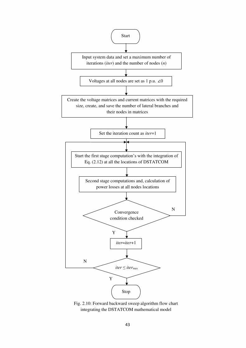
43

N

Y

N

Y

Start

Input system data and set a maximum number of iterations (iter) and the number of nodes (n)

Voltages at all nodes are set as 1 p.u. ∠0

Create the voltage matrices and current matrices with the required size, create, and save the number of lateral branches and

their nodes in matrices

Set the iteration count as iter=1

Start the first stage computation’s with the integration of Eq. (2.12) at all the locations of DSTATCOM

Second stage computations and, calculation of power losses at all nodes locations

Convergence condition checked

iter=iter+1

iter ≤ itermax

Stop

Fig. 2.10: Forward backward sweep algorithm flow chart integrating the DSTATCOM mathematical model

44

2.5. Conclusion

The essence of this chapter is devising a new phase angle model of DSTATCOM and

incorporating it in RDS to compensate the reactive power in the RDS. To understand the

modeling of DSTATCOM this chapter describes why DSTATCOM is required in RDS

and how it works to compensate the reactive power in RDS. The FBS load flow technique

is described clearly and its algorithm and flow chart are provided in this chapter. Mainly,

how the phase angle model of DSTATCOM can be injected in RDS via FBS load flow

algorithm is described elaborately in this chapter. This model is used in next all chapters

to solve the objectives the thesis.

45

Chapter 3 Reactive Power Compensation in Radial Distribution Systems with the Optimal Phase Angle Injection Model of Single

Distribution STATCOM 3.1. Introduction In this chapter, a distribution STATCOM (DSTATCOM) model based on optimal angle

injection is allocated optimally in RDS to compensate the reactive power. A DSTATCOM

is allocated at each bus of a distribution system, one at a time, and its impact on system

power loss and voltage profile are investigated. In the proposed DSTATCOM model, the

rating of the DSTATCOM is determined with the injection of optimal phase angle of the

voltage at the location, in which a DSTATCOM is placed. The proposed DSTATCOM

model is suitably incorporated in the forward-backward sweep load flow algorithm as

discussed in chapter 2. The optimal location and rating for DSTATCOM are determined

by minimizing the active power loss of a distribution network. Exhaustive search and

differential evolution algorithms are used as the solution strategy. The 30 and 69-bus radial

distribution system is used in the case study. The results show that the proposed approach

is more efficient in active power loss reduction as compared to some of the previously

published approaches.

3.2. Optimal allocation of DSTATCOM in RDS using exhaustive search algorithm

In this section, the optimal allocation of proposed phase angle model of DSTATCOM

in two different 30 and 69-bus RDS using exhaustive search method is presented. Firstly,

the objective function is formulated required in the approach proposed in this chapter.

Secondly, the operation of exhaustive search algorithm in proposed approach is described.

The incorporation of DSTATCOM in FBS load flow algorithm discussed in chapter 2 is

the main strategy to evaluate the load flow studies in this approach.

46

3.2.1. Objective Function

The placement of DSTATCOM is carried out to provide optimal reactive power

compensation by considering the operational constraints of the network. The modelling of

the DSTATCOM which is derived in chapter 2 is used to determine the optimizing

variables, such as optimal location(s) for DSTATCOM and the corresponding angle β'i+1

so as to get the lowest total active power loss as given below.

12

1

( ) ( )n

DSTATloss Brach

j

P I j R j

(3.1)

Where I Branch (j) and R (j) represent the branch/line current and the resistance of the branch

j, n is total number of buses in the RDS. This objective function is to be minimized under

the following constraints:

3.2.1.1.Voltage constraint

Voltage at each bus must be remained within the permissible range.

maxmini i iV V V (3.2)

Where Vi is the magnitude of the voltage at bus number i, Vimin min and Vi

max are the

minimum and maximum limits of the voltage at bus number i. Minimum voltage is taken

as 0.9 pu and maximum voltage limit is take as 1.05. If the voltage at bus i cross these

limits a penalty factor is added with the objective function given in Eq. (3.1)

3.2.1.2.Thermal constraint

The current flowing through each branch must be within maximum current carrying

capacity of the conductor.

maxj jI I (3.3)

Where Ij is the magnitude of the current flowing through the branch j and Ijmax is the

maximum limit of the current in the branch j. Maximum limit of the current is taken as 1.2

times the base current of the branch j. If the voltage and current of any bus or branch

violates these constraints, a penalty factor is added with the objective function in Eq. (3.1).

Hard constraints principle is used in this chapter.

47

3.2.2. Exhaustive search optimization method (ESM)

Exhaustive search technique is a general problem solving technique, which enumerates

each possible candidate systematically for the problem solution while keeping a check

whether each candidate solution is satisfying the statement of the problem or not [109].

Generally, this technique is used in discrete problems since these problems have no other

efficient techniques. However, the proposed problem has many techniques to solve. This

method can also be called as brute force method or direct search method or generate and

test method or British museum algorithm. Exhaustive search has two requirements that it

should be able to generate all candidate solutions and to check a candidate solution [110].

Also, generating and checking candidates should be efficient. A generalized pseudocode

for the exhaustive search method (ESM) is given in Table. 3.1 and ESM algorithm for the

proposed approach is given is Table. 3.2. ESM algorithm has the following advantages:

1) Its operation is simple

2) It can reduce the search space

3) It allows randomization so that the runtime gets improved

4) It is widely applicable, particularly to search-oriented problems

5) It is correct search method and gives correct generation and checking

Table.3.1: A generalized pseudocode for the exhaustive search algorithm:

Joseph (int NIT, int RKL)

If (is solution (NIT))

Print solution (NIT)

Else

NIT generated = generate solution ( )

Joseph (NIT generated, RKL+1)

48

Table.3.2: ESM Algorithm for proposed approach:

Require: Initialization of accuracy; maxiter; no. of nodes;

Require: Read the bus data and line data

Require: Create dummy matrices mat, V, X, and Rosh with required sizes in zeros/ones

for location=1:n

for cap=1:1:pahse angle or specified maximum limit of QDSTATCOM rating

for iter=1:maxiter

for j=n:-1:2

Ij=conj (complex(s (j, 1), s (j, 2)-QDSTATCOM)/V (1, j));

while (j<=n)

count=0;

if (count==1)

end node = j;

elseif (count==2)

end

break

end

end

if (max (abs (DIF))<=accuracy) %( check convergence)%

break

end

end

P loss /Q loss =0;

for b=1:n-1

Evaluate (P loss /Q loss)

end

Rosh (location, cap) = P loss /Q loss;

end

end

Print size of DSTATCOM; Plot minimum P loss /Q loss and voltage;

49

3.2.3. 69-bus RDS

Optimal allocation of phase angle model of DSTATCOM in 12.66kV, 100MVA, 69-bus RDS

[68] and [103] using exhaustive search algorithm is presented in this section.

3.2.3.1. DSTATCOM allocation strategy

In the modelling of the DSTATCOM derived in chapter 2 there is an unknown

parameter, i.e., the angle β' .This is the angular displacement of the voltage at the location

where a DSTATCOM is placed. This angle can vary between the limits 0 to 90 degrees.

In this work, three different values of β' are chosen to design to determine the current to

be injected by a DSTATCOM. They are:

Case A: Design of DSTATCOM with β'=18.4°

Case B: Design of DSTATCOM with β'=32.1°

Case C: Design of DSTATCOM with β'=68.4°

The respective reactive power to be injected by the DSTATCOM is obtained from Eq.

(2.12), chapter 2. In this work, a DSTATCOM is placed at each bus of the RDS one at

time and the system power loss is computed by incorporating the proposed model in the

forward-backward sweep load flow algorithm.

Initially, a constant voltage of all buses is assumed to be l p.u.∠0. Then, load currents

that are connected at all buses are calculated and line currents are determined by using in

backward sweeps. Thereafter, the voltage at each bus is computed in forward sweeps. Once

the new voltages at all buses are computed, the convergence criterion is checked. If it does

not converge, then load currents are evaluated using the most recent values of voltages and

the whole process is repeated till the convergence criterion is satisfied. The convergence

criterion is set as the maximum difference in magnitude of voltages in the consecutive

iterations is less than 1X10-3 p.u.

3.2.3.2.Simulation Result

In this section, the results of the computer simulation study are given to show the impact

of the allocation of phase angle model of DSTATCOM on RDS. The base case power loss

of the 69-bus RDS is 224.98 kW.

50

A. Impact of DSTATCOM Allocation on Network Loss

To study the impact of the DSTATCOM, it is placed in each bus, one at a time and the

power loss due to the DSTATCOM allocation is shown in Fig. 3.1. It is observed that there

is significant reduction in power loss at certain buses, for example at buses 11-20 and buses

52-61. The DSTATCOM location corresponding to the minimum power loss is found to

be bus 61. Thus, the voltage profile of the network with and without DSTATCOM

allocation at bus 61 is shown in Fig. 3.2. It is also observed that both power loss and voltage

profile are improved with a DSTATCOM designed with higher β'. Hence, better results

are found in Case C design of DSTATCOM. The power loss and percentage reduction in

power loss due to the DSTATCOM allocation at bus 61 are given in Table 3.1.

Table 3.3: Results obtained with DSTATCOM allocation at bus 61

B. Analysis of the VA rating of DSTATCOM

The VA rating for the DSTATCOM placed in different locations of the 69 bus test

system, one at a time is shown in Fig. 3.3. The results illustrate that higher-rated

DSTATCOM is required if it is to be placed closer to the substation. It is expected because

the branches located closer to the substation carry higher load current. It is also observed

that increase in angle of β' causes the requirement of a higher amount of shunt

compensating current in the compensation of reactive power. This is the reason of higher

VA rating of the DSTATCOM in planning Case C as shown in Table 3.1. Installation of

DSTATCOM by the proposed approach leads to 30.8% of power loss reduction in the 69-

bus RDS. The load flow results shows that power loss and voltage profile can be

significantly improved due to a DSTATCOM allocation.

Location

Case

β' (deg)

MVA rating

Power Loss (kW)

Power Loss reduction

(%)

61

Case A 8.4° 0.931 159.04 29.3%

Case B 32.1° 0.958 157.77 29.8%

Case C 68.4° 0.969 155.63 30.8%

51

Figure.3.1: Active power loss after installation of DSTATCOM in RDS

Figure.3.2: Voltage magnitude in different cases with DSTATCOM at bus 61

Figure.3.3: VA rating required for DSTATCOM in different locations of RDS

0 10 20 30 40 50 60 70150

200

250

300

DSTATCOM location

Act

ive

pow

er lo

ss (k

W)

Case ACase BCase C

0 10 20 30 40 50 60 700.9

0.92

0.94

0.96

0.98

1

Bus Number

Bus

Vol

tage

(p.u

.)

Base VoltageCase ACase BCase C

0 10 20 30 40 50 60 700

2

4

6

8

10

12

14

DSTATCOM location

VA

rat

ing

(p.u

.)

Case ACase BCase C

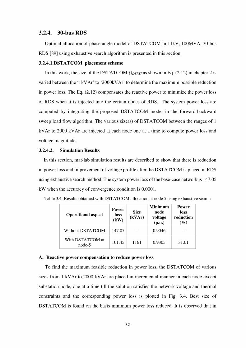
52

3.2.4. 30-bus RDS

Optimal allocation of phase angle model of DSTATCOM in 11kV, 100MVA, 30-bus

RDS [89] using exhaustive search algorithm is presented in this section.

3.2.4.1.DSTATCOM placement scheme

In this work, the size of the DSTATCOM QDSTAT as shown in Eq. (2.12) in chapter 2 is

varied between the ‘1kVAr’ to ‘2000kVAr’ to determine the maximum possible reduction

in power loss. The Eq. (2.12) compensates the reactive power to minimize the power loss

of RDS when it is injected into the certain nodes of RDS. The system power loss are

computed by integrating the proposed DSTATCOM model in the forward-backward

sweep load flow algorithm. The various size(s) of DSTATCOM between the ranges of 1

kVAr to 2000 kVAr are injected at each node one at a time to compute power loss and

voltage magnitude.

3.2.4.2. Simulation Results

In this section, mat-lab simulation results are described to show that there is reduction

in power loss and improvement of voltage profile after the DSTATCOM is placed in RDS

using exhaustive search method. The system power loss of the base-case network is 147.05

kW when the accuracy of convergence condition is 0.0001.

Table 3.4: Results obtained with DSTATCOM allocation at node 5 using exhaustive search

A. Reactive power compensation to reduce power loss

To find the maximum feasible reduction in power loss, the DSTATCOM of various

sizes from 1 kVAr to 2000 kVAr are placed in incremental manner in each node except

substation node, one at a time till the solution satisfies the network voltage and thermal

constraints and the corresponding power loss is plotted in Fig. 3.4. Best size of

DSTATCOM is found on the basis minimum power loss reduced. It is observed that in

Operational aspect Power

loss (kW)

Size (kVAr)

Minimum node

voltage (p.u.)

Power loss

reduction (%)

Without DSTATCOM 147.05 -- 0.9046 --

With DSTATCOM at node-5 101.45 1161 0.9305 31.01

53

Fig. 3.4 there exists a certain value of reactive power injected, in which power loss is

minimum, and it starts increasing beyond the value. The size of the DSTATCOM

corresponding to the minimum power loss, and the minimum node voltages due to

DSTATCOM integration in all nodes are given in Fig. 3.5, 3.6, and 3.7 respectively. The

results show that the minimum power loss is obtained at node 5 of IEEE-30 node RDN.

Figure.3.4: Variation of power loss with increment of DSTATCOM size in each node

Figure.3.5: DSTATCOM size corresponding to minimum power loss

B. Analysis of the power loss and voltage profile

There is an apparent impact of DSTATCOM on the network power loss as shown Fig.

3.4 and 3.6. Network power loss significantly reduced at almost all nodes. Mainly at the

0 5 10 15 20 25 30 350

500

1000

1500

2000

DST

AT

CO

M si

ze (k

VA

r)

DSTATCOM location (node)

54

nodes 3 to 7, 10 to 15, 20, 21, 28, and 30, power loss reduced between the range 19.75%

to 31.01%. It is observed that the highest percentage reduction in power loss occurred at

node 5 as 101.45 kW with the DSTATCOM size of 1161 kVAr as shown in Table.3.4.

Moreover, it is noteworthy that voltage also improved significantly compared to base case

voltage as shown in Fig. 3.8 after the placement of DTSTCOM at node 5. The

improvement in minimum node voltage and reduction in power loss due to the impact of

DSTATCOM placement at node 5 are provided in Table 3.4.

Figure.3.6: minimum power loss in each node due to integration of DSTATCOM

Figure.3.7: minimum node voltage due to the integration of DSTATCOM

0 5 10 15 20 25 30100

110

120

130

140

150

Pow

er lo

ss (k

W)

DSTATCOM location

0 5 10 15 20 25 300.905

0.91

0.915

0.92

0.925

0.93

0.935

0.94

Min

imum

m v

olta

ge m

agni

tude

(p.

u.)

DSTATCOM location (node)

55

Figure.3.8: Voltage magnitude with DSTATCOM at node 5

C. Analysis of the size of DSTATCOM

The size (rating) of the DSTATCOM placed in different locations of the 30 node RDN,

one at a time is shown in Fig. 3.5. This graph demonstrates that the size of DSTATCOM

is to be higher when it is placed nearby substation. Generally the branches of the RDN

which are near to substation carries higher load current and hence, it is estimated that the

shunt current that must be injected for the compensation of reactive power is to be higher

which consequently increases the size of the compensation device. Placement of

DSTATCOM by the proposed approach leads to 31.01 % of power loss reduction in the

IEEE-30 node RDN.

3.3. DSTATCOM Allocation Using DE

This section provides the objective function for the proposed planning problem for single

DSTATCOM allocation and the detailed solution strategy using DE.

3.3.1. DE: an overview

In this subsection, a brief overview on DE [98] is provided. DE is an efficient population-

based meta-heuristic search technique for solving problems of the global optimization by

using the operator’s mutation, crossover, and selection [99] - [101]. Firstly, the parameters

of DE algorithm are initialized, and then the target vector is generated. Secondly, the

mutant vector corresponding to each string of the target vector is produced by the operation

0 5 10 15 20 25 300.9

0.92

0.94

0.96

0.98

1

Node Number

Nod

e V

olta

ge (p

.u.)

Base voltage magnitudeVoltage magnitude with DSTATCOM

56

of mutation. Thirdly, the trial vector is generated by performing the crossover operation

between the target vector and its corresponding mutant vector. Fourthly, the trail vector is

generated after that, an operation of selection is executed. The population consists of Np

individual strings and each individual has a dimension D equals to the number of

optimizing variables. The initial population generated is randomly generated under the

limits of optimizing variables. The population in subsequent generations are evolved by

the application of evolutionary operators, such as mutation, crossover, and selection till

the termination criterion is satisfied. The evolutionary operators are briefly described

below. The flow chart of DEA is shown in Fig. 3.9.

Step 1. Initialization: Number of strings as population Np, and the dimension (D) of

optimization variables in each individual string, so called target vector (TG) are initialized

and randomly generated by

max, min min . ( )j j jji GenTG round TG TG TG rand (3.4)

Where, i = 1,2,…,Np ; j = 1, 2,…,D and Gen is the generation number.

Step 2. Mutation: In each generation, for each target vector TG ji,Gen

, a mutant vector

MUTi,Gen is produced by the following equation:

1 2, , , , . i Gen best Gen r Gen r GenMUT TG F TG TG (3.5)

r1, r2 are individual integers that are generated randomly between the ranges [1, Np]. These

integers are generated once for each mutant vector. The weighting factor F is a positive

number for scaling the difference vector which is constant in the range 0 to 2. TG best is the

best target vector according to the objective (fitness) function value in the population at

that particular generation Gen.

Step 3. Crossover: after the accomplishment of operation of mutation, the operation of

crossover is required to be performed on each and every pair of the target vector TGi,Gen

and its corresponding mutant vector MUTi,Gen for the generating a trial vector CROSji,Gen

using the following equation:

57

,,

,

j i Genj i Gen

j i Gen

MUT if rand CRCROS

TG otherwise

(3.6)

where, CR is the cross over rate which is called as crossing factor and it is an user-defined

parameter between range of [0, 1]. Crossing factor controls values that are available from

the mutant vector.

Step 4. Selection: Selection is an operation which will be performed after the crossover. .

Before this operation is performed, it is an important thing to be noted that, “If the values

of string variables of a newly generated trial vector exceed the corresponding upper and

lower limits, then these variables are reinitialized randomly within the pre specified limits.

Then, the fitness function values of all trial vectors are computed. After that, a selection

operation is performed. The fitness (objective) function value of each trial vector f (CROS

j i, Gen) is compared with the respective target vector f (TG j i, Gen) in the current population.

If the trial vector has less or equal fitness (objective) function value than the respective

target vector, then the target vector will be replaced by the trial vector and entered the

population of the coming generation. Otherwise, in the coming generation the target vector

would be remained in the population. The operation of selection is as follows:

, , ,, 1

,

( ) ( )i Gen i Gen i Geni Gen

i Gen

CROS if f CROS f TGTG

TG otherwise

(3.7)

Where f is the fitness function, i.e., the objective function shown in Eq. (3.1). The above

steps, i.e., mutation, crossover and selection are repeated in each generation until the

population is converged to an optimum value.

3.3.2. Proposed Solution Strategy Using DE

In the proposed scheme, a typical string for DE consists of the information of location

for DSTATCOM and the phase angle β'i+1 (derived in chapter 2). All the busses except the

substation bus are considered as candidate location for DSTATCOM and the range for the

phase angle β'i+1 should lie in between 0 to 90 degrees.

58

3.3.3. Proposed DE algorithm

Algorithm:

Step 1: Initialize number of population=NP=50; size of the string=D=7; maximum

generation=100; F= 0.5; CR= 0.6;

Step 2: Create dummy matrices to save the results of optimal location, optimal phase

angle, and optimal power loss during the operation of Target vector (TG), Mutant vector

(MUT) and trail vector (U).

Step 3: Initialize the lower limit (LT) and upper limit (UL) of optimal location and phase

angle.

Step 4: Generate ‘TG’ (populations) with 50 strings in the format as shown in Fig.4.2

whose variables are randomly chosen according to the following equation

TG (POP, D) = round (LT+ ((UT-LT)* rand ()));

Step 5: Run the FBS load flow algorithm as described in “Algorithm” given in chapter 2

for each string of ‘TG’ and evaluate the power loss according to the Eq. (3.1)

Step 6: Generate ‘MUT’ (population) using the operation of mutation by mutating the

variables in each string of ‘TG’ for ‘100’ generations according to the following equation

MUT (POP, Variable) =abs (floor (TG (R0, Variable) +F*((TG (R1,

Variable))-(T (R2, Variable)))));

Where R0 =ceil (NP*rand ()); while (R0=POP)

R1=ceil (NP*rand ()); while (R1=R0||R1=POP)

R2=ceil (NP*rand ()); while (R2=R1||R2=R0||R2=POP)

F= weighting factor

Step 7: Repeat step 5 for each string of ‘MUT’

Step 8: Generate ‘U’ (population) using the operation of crossover for ‘100’

generations according to the following statements

if ((rand()<=CR)||(D=Drand))

U(POP,D)=MUT(POP,D);

else U(POP,D)=TG(POP,D);

end

Where Drand=ceil(1+(rand*3));

CR=Crossover Rate

Step 9: Repeat step 5 for each string of ‘U’.

59

Step 10: Select the best (optimal) location, value of phase angle based on the best

minimum power loss through the operation of ‘selection’ as given below

if (U_Ploss(POP) <= TG_Ploss(POP))

TG (POP, :) = U (pop, :);

else TG (POP, :) = T (POP, :);

end

Where U_Ploss = Power loss corresponding to each string of

Trial vector (MUT)

TG_Ploss = Power loss corresponding to each string of

Target vector (TG)

Step 11: End

Step 12: Print optimal result

3.4. Simulation Results

In this section, the simulation results are presented to show the impact of the allocations

of single DSTATCOM in the network to minimize the active power loss. The active and

reactive power loss of the base-case network is 224.98 kW and 102.1 kVAr respectively.

The parameters of DE algorithm are optimized by taking repetitive runs and the optimal

parameters are shown in Table 3.5. Firstly, the ESM algorithm is applied to know the

optimal location and rating of DSTATCOM. In this method the optimal variable phase

angle β'i+1 is injected in RDS through FBS from 0º to 90º in an incremental manner. The

corresponding powerless to injection of each angle of β'i+1 have been recorded. Secondly,

the DE algorithm is used to optimize the objectives of the proposed approach in this

chapter.

Table 3.5: Parameters of DE algorithm

DE parameters Values

Population size 50

Maximum Generation 100

Crossover rate 0.6

Weighting factor 0.5

60

Figure.3.9: Flow chart of proposed DE algorithm

N

Y

Initialize the variables and parameters of DE and generate target vector (TG) using Eq. (3.4)

Run the forward-backward load flow algorithm and compute the fitness (power loss) for each string of ‘TG’

Generate mutant vector (MUT) using Eq. (3.5) and compute fitness function (power loss) using load flow algorithm

TGen+1 = UGen

Gen > Max Gen

Gen=Gen+1

Start

k=1

k=NP

Print the optimal solution

k=k+1

f(UGen) ≤ f(TGen)

TGen = TGen+1

N

Y N

Generate trial vector (U) using Eq. (3.6) and compute fitness function (power loss) using load flow algorithm

Stop

Y

61

3.4.1. Results of Exhaustive Search

Firstly, an exhaustive search, in which a DSTATCOM is placed in each node, except

the substation node, one at a time, is carried out. To determine the optimal DSTATCOM

location and rating, the phase angle β'i+1 is varied from zero to 90 degree and the

corresponding active power loss is plotted in Fig. 3.10. It is observed that the active power

loss initially decreases with increase in phase angle β'i+1 and there exists a certain value of

phase angle for DSTATCOM, in which the network active power loss is minimum and it

starts increasing beyond the value. This shows the need of considering the phase angle β'i+1

as an optimizing variable.

Figure.3.10: Variation of active power loss with increment of phase angle β'i+1 in each bus

The rating of DSTATCOM corresponding to the minimum active power loss, the value

of minimum active power loss, the minimum bus voltages with DSTATCOM allocation

in all buses and the value of minimum reactive power loss are given in Figs. 3.11, 3.12,

3.13, and 3.14 respectively. The phase angle corresponding to the minimum active power

loss varies depending on DSTATCOM locations. In most of the locations, the variation

lies between 20-30 degrees. The results show that the minimum active power loss can be

obtained if a DSTATCOM is placed in bus 61.

0 10 20 30 40 50 60 70 80 90 100150

200

250

300

Variable phase angle (degree)

Pow

er l

oss

(kW

)

62

Figure.3.11: DSTATCOM rating in kVAr corresponding to minimum active and reactive power loss

Figure.3.12: Minimum active power loss in each node due to DSTATCOM

0 10 20 30 40 50 60 700

500

1000

1500

2000

2500

3000

3500

DSTATCOM location

DST

ATC

OM

rat

ing

(kV

Ar)

0 10 20 30 40 50 60 70150

160

170

180

190

200

210

220

230

DSTATCOM Location

Min

imum

act

ive p

ower

loss

(kW

)

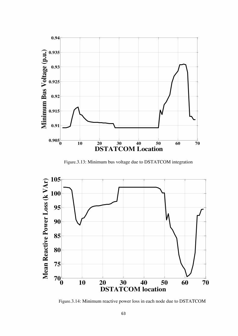
63

Figure.3.13: Minimum bus voltage due to DSTATCOM integration

Figure.3.14: Minimum reactive power loss in each node due to DSTATCOM

0 10 20 30 40 50 60 700.905

0.91

0.915

0.92

0.925

0.93

0.935

0.94

DSTATCOM Location

Min

imum

Bus

Vol

tage

(p.u

.)

0 10 20 30 40 50 60 7070

75

80

85

90

95

100

105

Mea

n R

eact

ive

Pow

er L

oss (

k V

Ar)

DSTATCOM location

64

3.4.2. Results of DSTATCOM allocation using DE

The proposed algorithm is used in the determination of the optimal allocation of single

DSTATCOM. The active power loss corresponding to the best solution in each generation

of DE with single DSTATCOM allocation is shown in Fig. 3.15. It is observed that the

minimum power loss from generation to generation from 1st to 11th generation has been

reduced. After the 11th generation minimum power are converged beyond which the

minimum power loss remains same. The time to get convergence of an objective function

seems very less in DE algorithm. The same can be observed in the rest of the DE based

simulation results. Therefore, DEA is very fast and effective evolutionary algorithm to

optimize the variable of fitness function. The mean active and reactive power loss of the

population in each generation of DE is shown in Fig. 3.16. and Fig. 3.17 respectively. The

minimum active and reactive power loss are found to be 152.04 kW and 70.56 kVAr

respectively with a 27.49º optimal phase angle injected by DSTATCOM allocation at bus

61. It is attention grabbing that the optimal phase angle obtained by ESM algorithm found

to be almost same in Fig. 3.10 compared to the DE based algorithm.

Figure.3.15: Minimum active power loss of each generation with single DSTATCOM allocation

65

Fig. 3.16: Mean active power loss of each generation with DSTATCOM allocation

Fig. 3.17: Mean reactive power loss of each generation with DSTATCOM allocation

0 10 20 30 40 50 60 70 80 90 100150

160

170

180

190

200

210

220

230

240

250

Generation (iteration)

Mea

n A

ctiv

e P

ow

er L

oss

(k

W)

0 10 20 30 40 50 60 70 80 90 10070

75

80

85

90

95

100

105

110

115

Mea

n R

eact

ive

Pow

er L

oss

(k V

Ar)

Generation (iteration)

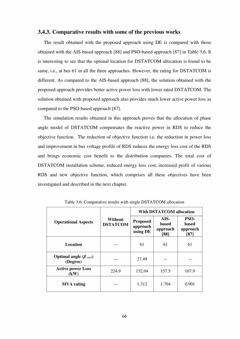
66

3.4.3. Comparative results with some of the previous works

The result obtained with the proposed approach using DE is compared with those

obtained with the AIS-based approach [88] and PSO-based approach [87] in Table 3.6. It

is interesting to see that the optimal location for DSTATCOM allocation is found to be

same, i.e., at bus 61 in all the three approaches. However, the rating for DSTATCOM is

different. As compared to the AIS-based approach [88], the solution obtained with the

proposed approach provides better active power loss with lower rated DSTATCOM. The

solution obtained with proposed approach also provides much lower active power loss as

compared to the PSO-based approach [87].

The simulation results obtained in this approach proves that the allocation of phase

angle model of DSTATCOM compensates the reactive power in RDS to reduce the

objective function. The reduction of objective function i.e. the reduction in power loss

and improvement in bus voltage profile of RDS reduces the energy loss cost of the RDS

and brings economic cost benefit to the distribution companies. The total cost of

DSTATCOM installation scheme, reduced energy loss cost, increased profit of various

RDS and new objective function, which comprises all these objectives have been

investigated and described in the next chapter.

Table 3.6: Comparative results with single DSTATCOM allocation

Operational Aspects Without DSTATCOM

With DSTATCOM allocation

Proposed approach using DE

AIS-based

approach [88]

PSO-based

approach [87]

Location --- 61

61

61

Optimal angle (β' n+1)

(Degree) --- 27.49 -- --

Active power Loss (kW) 224.9 152.04 157.5 167.9

MVA rating --- 1.312

1.704

0.901

67

3.5. Conclusion

In this paper, the proposed DSTATCOM model is incorporated into the

Forward/backward sweep load flow algorithm so as to study its impact on the network

active and reactive power loss and voltage profile. The 30, 69-bus RDS are used in the

case study. The study shows that the network active and reactive power loss can

significantly be reduced with a DSTATCOM placement at optimal location with optimal

phase angle. Two-optimization approaches ESM and DE have been proposed to determine

the optimal location and size for DSTATCOM. The study reveals that significant active

and reactive power loss reduction is possible with a DSTATCOM allocation at optimal

location with optimal phase angle in a distribution systems. In comparison with some of

the previously published works, the allocation of the proposed DSTATCOM model results

in comparatively lower active power loss.

68

Chapter 4 Optimization of Planning Cost of

Distribution Systems with the Optimal Placement and Sizing of DSTATCOM Using Differential Evolution Algorithm

4.1. Introduction

This chapter presents an optimization of planning cost of DS with the optimal allocation

and sizing of DSTATCOM using DEA. In this appraoch the optimization of planninng

cost of DS comprises optimization of energy loss cost (ELC) of DS, and the optimal

allocation and sizing of DSTATCOM to maximizing the total net profit (TNP)/cost savings

per annum and planning horizon (PH) of DSTATCOM installation scheme. In this

approach, the optimal reactive power compensation is the main vital role in solving the

objective function. The optimal reactive power compensation with the optimal placement

and sizing of DSTATCOM and the improvement in voltage profile of the DN are obtained

based on certain objectives such as best reduction in network power loss and the total ELC

and the maximization of TNP. A new phase angle modeling on the size of DSTATCOM

was incorporated in DN through the forward-backward sweep load flow technique as

described in chapter 2 to evaluate the parameters of load flows in DN. Present worth factor

(PWF) is instigated to evaluate the TNP of the DSTATCOM installation scheme. The

proposed method is validated on the 30-bus, 33-bus, and 69-bus RDS. The simulation

results obtained in this approach are compared with the some of the previous investigations

and found to better.

4.2. Importance of Planning

In order for the industry to remain profitable, the principal company must obtain the

least amount of total cost of ownership. This means selecting system configurations with

low cost by also accounting for cost of operation, maintenance & upgrades, and system

decommissioning. Planning is necessary to design a system for optimum performance.

69

While ensuring supply continuity, minimizing power losses, ensuring power quality, and

obtaining trouble free operation by selecting appropriate sizing equipment based on

surrounding influences. The planning of electric power distribution in buildings and

infrastructure facilities is subject to constant transformation. The search for an assignment-

compliant, dependable solution should fulfil those usual requirements placed on cost

optimization, efficiency, and time needs.

4.3. Planning for Industrial Distribution Systems

Planning begins with assessing the predetermined energy demand for the facility. To

understand what the facility would require for energy consumption prior information of

other facilities projects with similar equipment and processes is a good starting point. This

only provides a starting point, where a better approximation can be determined based on

facility machinery and equipment. Data required to be collected for power estimation

include:

1. List of connections loads and locations

2. Pattern of loading (process variations)

3. Separating critical load from non-critical loads

4. Loads with high harmonics

5. Inclusion of future growth plans

6. Utility interfacing

A list of load locations and pattern of equipment loading will aid in assessing the load

factor, demand factor, and diversity factor. Application of these factors is crucial in

accurately estimating power requirements for any facility and designing distribution

systems.

Power distribution systems require large amounts of funds for investments in any industry

and a sizeable amount for operational costs. Proper planning for designing a distribution

system with optimum performance requires several steps from collecting data, selecting

proper configurations, and selecting appropriate equipment using planning tools, and

software for modeling and documenting important aspects of the distribution system.

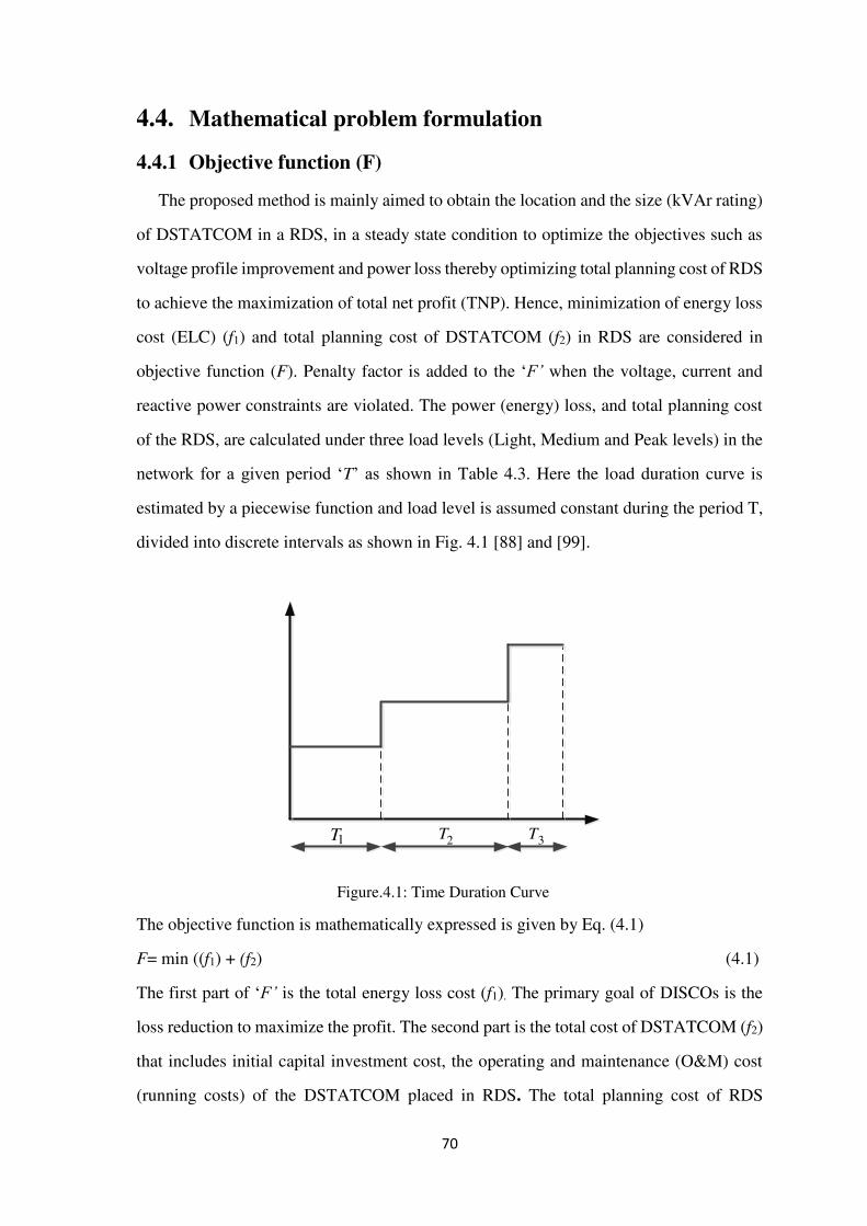
70

4.4. Mathematical problem formulation

4.4.1 Objective function (F)

The proposed method is mainly aimed to obtain the location and the size (kVAr rating)

of DSTATCOM in a RDS, in a steady state condition to optimize the objectives such as

voltage profile improvement and power loss thereby optimizing total planning cost of RDS

to achieve the maximization of total net profit (TNP). Hence, minimization of energy loss

cost (ELC) (f1) and total planning cost of DSTATCOM (f2) in RDS are considered in

objective function (F). Penalty factor is added to the ‘F’ when the voltage, current and

reactive power constraints are violated. The power (energy) loss, and total planning cost

of the RDS, are calculated under three load levels (Light, Medium and Peak levels) in the

network for a given period ‘T’ as shown in Table 4.3. Here the load duration curve is

estimated by a piecewise function and load level is assumed constant during the period T,

divided into discrete intervals as shown in Fig. 4.1 [88] and [99].

Figure.4.1: Time Duration Curve

The objective function is mathematically expressed is given by Eq. (4.1)

F= min ((f1) + (f2) (4.1)

The first part of ‘F’ is the total energy loss cost (f1). The primary goal of DISCOs is the

loss reduction to maximize the profit. The second part is the total cost of DSTATCOM (f2)

that includes initial capital investment cost, the operating and maintenance (O&M) cost

(running costs) of the DSTATCOM placed in RDS. The total planning cost of RDS

1T 2T 3T

Light load levelMedium load levelPeak load levelTime (hour/year)Power (kW)

71

depends on the amount of power loss reduction, which is absolutely depended on the size

of DSTATCOM allocated optimally on the network. However, the installation of

DSTATCOM increases the planning cost. Therefore, the objective of optimal

DSTATCOM placement problem, in this case, is to minimize the total cost for planning

the RDS and is defined by the Eq. (4.2). [83], [111]

Objective function= F =( f1 + f2 ) × [PF] (4.2)

1 1 1

ph nlDSTAT DSTATf E C P T PWF PFLoss Cost e Loss kky k

(4.3)

2 21 22 23f DSTAT f f f PFTotal Cost (4.4)

( )21 1

nl DSTATf k C Q PWFck in kk

(4.5)

( )22 1 1

ph nl DSTATf k C Q PWFck op ky k

(4.6)

( )23 1 1

ph nl DSTATf k C Q C PWFck in k may k

(4.7)

Where ‘PF’ is the penalty factor shown in Eq. (4.12), f21, and f22 and f23 are the total initial

capital investment cost and the total operational cost and the total maintenance costs of the

DSTATCOM respectively in the whole PH of DSTATCOM installation scheme. The f21

is considered per year in three load levels since it is installed only once for the total

planning horizon. Ce is the energy cost per kWh; Tk is the duration of time in kth load level;

Cin is the initial capital investment cost(purchase cost) of DSTATCOM per kVAr; Cop is

the operational cost of the DSTATCOM per kWh; Cma is the DSTATCOM maintenance

cost which in terms of the % of initial cost of DSTATCOM per a year; QkDSTAT is the size

of the DSTATCOM placed at optimal location during kth load level ; kck is the

proportionality constant of kth load level time duration to the total duration of the time

formulated as following Eq. (4.8)

72

1

Tkkck nlTkk

(4.8)

4.4.2 Real power loss

The optimal variables, such as optimal location for DSTATCOM and the

corresponding size through the optimal angle β'n+1 are determined by Eq. (2.11) to get the

lowest total power loss and improvement in the voltage profile. The real power loss

encountered in Eq.(3.1) is expressed by Eq. (4.9). [97].

1 2( ) ( )1 1

nl nDSTATP I j R jLoss b bk k j

(4.9)

Where is the active power loss during kth load level after DSTATCOM is

installed, nl is the number of load levels given in Table 4.3, k is the load level, n is the total

number of buses in the DN, Ib (j) and Rb (j) are the line current and the resistance of jth

branch respectively.

4.4.3 Present worth factor (PWF) analysis

To evaluate the economic value of the DSTATCOM installation scheme, it is required

to compare the expected revenue and investment costs over the whole PH of DSTATCOM

installation scheme. In the proposed objective function as given in Eq. (4.3), the PWF

principle is adopted for cost-benefit analysis of the scheme. The PWF offers a net worth

of the scheme in today’s dollars by discounting each year’s cash flow back to the present

and then, deducing the initial investment. The mathematical expression of PWF is

expressed by Eq. (4.10): [112]-[114].

1

1 1

yPWF

y

(4.10)

Where y is the total planning horizon, γ is the discount rate of interest considered as 10%

for each annual period. The total cost of energy loss, initial capital investment, operational

and maintenance costs of DSTATCOM placed at interest, compounded annually at γ

percent for ‘y’ years equals to the PWF. In another words, the PWF is simply the reciprocal

k

DSTATlossP

73

of the foregoing compounding factor. It is inescapable that if we provide for a return we

must also discount all future costs. It must be noted that the PWF does not imply an

appraisal of assets in terms of present day reproduction costs. The PWF principle can

appraise a long-term plan with the following advantages.

It can compare the costs and benefits in a logical manner by recognizing the time

value of money

It can adjust the discount rate or expected cash flows in order to incorporate any

risk into the valuation of a planning

4.4.4 TNP/Savings:

The TNP which is to be maximized is the difference between the expenditure of the

energy loss cost of a DN without DSTATCOM and the total expenditure of the energy loss

cost of a DN with the scheme of DSTATCOM. It is given by the Eq. (4.11). [88]

1/

11 1

ph nl w o DSTATTNP C P T Fe Loss k yky k

(4.11)

TNP, in fact, yields an economic savings or benefit in the DN with DSTATCOM for the

total PH of DSTATCOM installation scheme, [99] and [102]. Therefore, the purchasing

cost of power from substation according to the customer's demand can be reduced.

4.5 Constraints

The proposed Eq. (4.3) is bounded by various active constraints to meet the limitations

on DSTATCOM operation and electrical requirements for the DS. Penalty factor is

considered when the objective functions f1 and f2 are converged as a single objective

function and the operating variables such as bus voltages, line currents and the capacity of

the DSTATCOM violates the desired safe limits. The soft constraints princple is used in

this appraoch to to introduce penalty factor. The minimum and maximum voltages are

considered as 0.9 p.u. and 1.1 p.u. respectively[88] as shown in Table 4.1. If the voltage

at bus i cross these limits the penalty factor is considered in objective function Eq. (4.3).

Maximum limit of the current in the network is taken as 1.2 times the base current of the

branch j. The line will be melted if the maximum limit of the current exceeds. The

74

maximum capacity of is considered as 10000 kVAr beyond which the penalty factor is

considered. The constraints are taken in steady state. The penalty factor used in proposed

objective function is given by Eq. (4.12).

1( )

1 1 1

nl n nover overPF Penalty Factor I j Vb nk j j

(4.12)

Where

1; ( ) ( )

( ) ( )exp 1 ; ( ) ( )

( )

Maxif I j I jb boverI j I jb Maxb if I j I jb bMaxI jb

(4.13)

1;

exp 1 ;

Min Maxif V V Vn n noverVn V Orelsen

(4.14)

Penalty factor is used to minimize the deviation of node voltage and line current.

‘Ibover(j)’ is the factor of over current flowing through the branches (lines) and ‘Vn

over ’ is

the over voltage factor. λ and µ are small positive constants. If branch currents ‘Ib (j)’ are

less than ‘Ibmax(j)’, then ‘Ib

over(j)’ will be equal to one. Similarly, ‘Vnover ’ will be equal to

unity when bus voltages are within the desired limits. In all other conditions, ‘Ibover(j)’ or

‘Vnover ’ shall attain a value (greater than unity) that acts as a penalty factor in objective

function Eq. (4.3).

The penalty factor method is an effective constraint handling technique, and it can

guide infeasible solutions to move to feasible solutions [115] i.e. it convert a constraint

optimization problem into a non-constrained optimization problem when it was added for

violation of constraints. In this paper, we adopt a common penalty function method [88]

and [116] to handle constrained optimization problems as shown in Eqs (4.12)-(4.14). The

75

λ and µ in Eqs (4.13) and (4.14) are the small positive constant, and represents the tolerated

violation, which imposes penalty on unfeasible solutions. These both constants are set to

0.1 to punish constraint violations [88]. If the penalty value is very high, the feasible region

will be approached mostly at random and the feasible global optimum will be hard to get.

On the other hand, if the penalty is too low, the probability of not reaching the feasible

region will be high. Therefore, the penalty factors must be carefully tuned, as they are

problem-dependent. The penalty factor used in proposed approach is taken from IA

approach [88] since the effectiveness and performance of proposed approach is compared

mainly with IA approach [88].

Table 4.1: Constraints considered in proposed approach

S.No Name of the constraint Range Min

limit Max limit

1 Voltage maxminkk kV V V 0.9 p.u. 1.1 p.u.

2 Current maxk kI I -- 1.2 times base

Ij p.u.

3 Reactive power min

11 1max

DSTAT DSTATkk kQ Q Q -- 10000kVAr

Table 4.2: Parameters of DEA

NP D F CR Generations

50 2 1 0.8 100

Figure.4.2: A typical string for DEA

Value of θ'i+1 corresponding to the

location of DSTATCOM

N β'n+1, N (which yields QDSTAT)

Location of DSTATCOM

76

The final aim is to minimize the proposed objective function so that all boundary

conditions be satisfied. If the solution violates the proposed constraints for the particular

candidate locations to obtain the best solution, then it will cause the drastic increase in the

value of objective function, which lead to an inappropriate solution [88]. The minimization

of objective function enhances the bus voltage profile. However, it should not be enhanced

beyond the magnitude of 1p.u. because the power loss in distribution systems are more

than transmission systems, which cause the huge drop in the magnitude of the bus voltage

as mentioned in section I. Thus, the compensation of reactive power in distribution systems

can never enhances the magnitude of the voltage to the value beyond the magnitude of

source voltage of the distribution system. However, it may happen when the concept of

constraints optimization is not considered in the optimization algorithm, which results the

requirement of higher amount of reactive power compensation. Hence, the magnitude of

bus voltages obtained in the proposed approach are found to be appropriate since the

constraints are imposed. For example, the magnitude of bus voltages as shown in Figs.

(4.12), (4.13), (4.16), (4.17), (4.20), and (4.21) have not crossed the voltage magnitude of

1p.u.

Figure.4.3: Typical IEEE 30-bus DN

14 15 16 17

18

87 96543

1920 21 22

21

2524

23

26 27

121110 13

302928

77

Figure.4.4: Typical IEEE 33-bus DN

121110 1413 15 16 17 1887 96543

302928 33

5251

3231

19 20 21 222

47 4948

1 252423

66 67

34

26 27

35

53 54 55 56 57 58 59 60 61 62 63 64 65

68 69

50

36 37 38 39 40 41 42 43 44 45 46

Figure.4.5: Typical IEEE 69-bus DN

121110 1413 15 16 17 1887 96543

302928 3326 27 3231

19 20 21 22

2

24 2523

1

78

4.6 Solution Strategy Using DEA

The main purpose of the DEA in this approach is the minimization of an objective

function given in Eq. (4.2) by determining the capacity of the DSTATCOM at the

candidate locations. A typical string structure is shown in Fig. 4.2. The candidate locations

for DSTATCOM are considered to be all the busses for each load level except the

substation bus and the range for the angle β'n+1 should lie in between 0 to 90 degrees. The

optimal value of β'n+1 decides the optimal size of DSTATCOM with the help of Eqs. (2.11)

and (2.12) in chapter 2.

Table 4.3: Load duration time and load level

Load level Light load Medium load Peak load

Time duration (hour/year) 2000 5260 1500

Total Load (kVA)

30-Bus 1603.2+j1196.4 2084.1+j1196.4 2306.7+j1196.4

33-bus 3715+j2300 4829.5+j2300 5944+j2300

69-bus 3802+j2694.6 4942.8+j2694.6 6083.5+j2694.6

Total power loss (kW)

30-bus 146.07 220.32 320.02

33-bus 202.66 305.81 442.39

69-bus 224.97 342.96 502.47

To study the validity of the proposed approach, three standard sample RDS such as 30,

33 and 69 bus networks are taken [117], [88] and their typical single line diagrams are

shown in Figs. 4.3, 4.4 and 4.5 respectively. To assess the virtue of DEA it has been

compared with an approach based on IA [88] in view of performance and run on the same

parametrical basis. The DEA parameters initial population size (NP), dimension of each

population (D), weighting factor (F), crossover rate(CR), and maximum generations, are

taken as mentioned in Table 4.2. Initial strings that are produced randomly, contains bus

location for compensation as well as optimal variable angle β'n+1 of DSTATCOM for the

respective location at all(three) load levels. The objective function is calculated for each

string by running Load flow algorithm at all load levels. The fitness (objective) function

parameters used in this work are shown in Table 4.4 [88], [118]. The mutation can not

guarantee the solutions with the specified range of two different string variables since there

is a strong mutual dependence of two variables while encoding the problem. Moreover,

79

the proposed algorithm is a probabilistic algorithm. Hence, to evaluate the performance of

proposed algorithm, 50 runs are performed and corresponding suboptimal solutions are

obtained. Thus, after the statistical computations the mean value and standard deviation of

the total energy loss cost with DSATCOM (f1) and the total planning cost (F) for the

optimal solution obtained with 50 runs are obtained and are given in Table 4.9. The best

values of the active power loss, the total energy loss cost with DSATCOM (f1), and the

total planning cost (F) among these 50 runs have been considered respectively as the best

solution as shown in Figs. (4.8), (4.9), (4.10), and Tables 4.5, 4.6, and 4.7. In IA algorithm

[88], the number of populations, generations and runs are taken as 50, 100, and 50

respectively. The same parameters have been considered in this approach as given in Table

4.2 to show the performance of proposed approach. The computing time of these two

algorithms are compared in Table 4.10. It should be noted that the constraint of injected

reactive power by DSTATCOM, voltage at each bus and current in each line are

considered as steady state as mentioned in subsection 4.4.1 of section 4.4.

4.7 Simulation results

In this section, the impact of DSTATCOM on total ELC of the DN per annum and PH

of DSTATCOM installation scheme, under three load levels are analyzed. The usefulness

of proposed approach is demonstrated on three RDS as mentioned in section 4.6. Three

load levels are selected as referred in subsection 4.4.1 of section 4.4 to model the annual

load profile. The time duration, total load for each load level, and base power loss in three

load levels are shown in Table 4.3.

Table 4.4: Parameters of objective function

Objective function parameter Value

Number of load levels 3

Cost of energy loss(ke) US($/kWh) 0.06

Cost of DSTATCOM(kin) US($/kVAr) 50

Operational cost of DSTACOM(kop) US($/kWh) 0.02

Maintenance cost of DSTACOM(kma) US($/kWh) 0.05

Discount rate of interest (γ) 0.1

PH (years) 30

80

Table 4.5: Comparative results of reactive power compensation with DSTATCOM for three load levels

Test network Approach

Light load level Medium load level Peak load level

Optimal location

Optimal size

(kVAr)

Power Loss (kW)

Min voltage (p.u.)

Optimal location

Optimal size

(kVAr)

Power Loss (kW)

Min voltage (p.u.)

Optimal location

Optimal size

(kVAr)

Power Loss (kW)

Min voltage (p.u.)

30-bus Proposed 5 1159.6 100.8 0.9358 5 1204.9 166.7 0.9189 5 1271.3 261.2 0.8888

33-bus

Proposed 30 1252.7 143.5 0.9256 30 1278.4 241.2 0.9058 30 1314.0 370.4 0.8832

IA [88] 12 962.4 171.8 -- 12 1008.1 272.0 -- 12 1222.6 407.7 --

GA [88] 12 1114.2 173.9 0.9272 12 1376.9 281.4 0.9120 12 1845.4 440.5 0.8977

69-bus

Proposed 61 1312.1 152.0 0.9338 61 1360.8 261.9 0.9124 61 1404.0 410.5 0.8899

IA [88] 61 1704.4 157.5 -- 61 1911.2 274.4 -- 61 2606.8 472 --

DE [57] 61 924.0 158.6 0.9246 -- -- -- -- -- -- -- --

GA [88] 61 1918.3 165.4 0.9392 61 2223.2 292.1 0.9209 61 2883.0 502.6 0.9061

PSO [87] 61 1901.0 167.9 0.9389 -- -- -- -- -- -- -- --

81

4.7.1 Impact of DSTATCOM allocation

When DSTSTCOM is allocated one at a time at each bus except substation bus, there

is a significant reduction in power loss and an improvement in minimum bus voltage of

the DS at some certain buses. Figs. 4.11 and 4.12 show the impact of DSTATCOM on

power loss and minimum bus voltage of IEEE 30-bus DN respectively, and It is observed

that these parameters have been affected much when DSTATCOM is placed at buses 3-7,

10, 14, 20 and 21. The DSTATCOM location corresponding to the minimum power loss

is found to be bus 5. Thus, the voltage profile of the network with and without

DSTATCOM allocation at bus 5 is shown in Fig. 4.13. Similarly, Figs. 4.15 and 4.16

demonstrate the impact of DSTATCOM on power loss in IEEE 33-bus DN respectively.

Table 4.6: Comparative results of annual cost of RDS with DSTATCOM installation without

considering operational and maintenance cost of DSTATCOM

Test network

Total energy loss cost without DSTATCOM($)

Approach F ($) TNP

($) f1 ($) f21 ($)

30-bus 1,16,374 Proposed 89,127 6,399 20,848

33-bus 1,60,670

Proposed 1,26,679 6,780 27,211

IA [88] 1,43,160 5,989 11,521

GSA [119] -- -- 12389

69-bus 1,80,470

Proposed 1,37,841 7,198 35,431

IA [88] 1,47,980 10,518 21,972

GSA [119] -- -- 12837

Table 4.7: Results of total costs considering PWF for PH of DSTATCOM installation scheme,

including operational and maintenance cost of DSTATCOM

Test network

Total energy loss cost without

DSTATCOM($)

F($) TNP ($)

TNP (%) f1($) f2($)

30-bus 6,99,570 5,32,630 6,861 1,60,078 22.88%

33-bus 9,69,976 7,64,873 7,275 1,97,827 20.39%

69-bus 10,89,530 8,32,268 7,722 2,49,540 22.90%

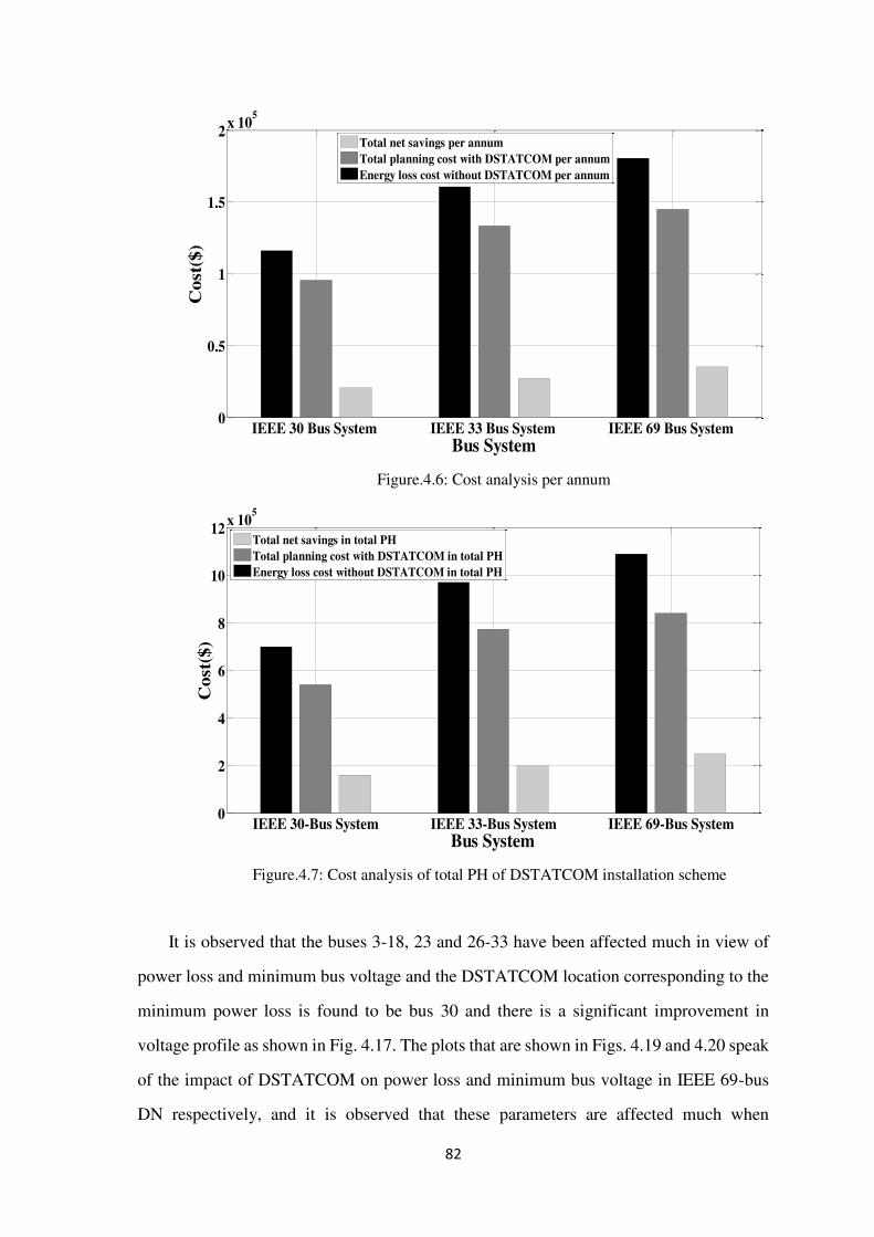
82

Figure.4.6: Cost analysis per annum

Figure.4.7: Cost analysis of total PH of DSTATCOM installation scheme

It is observed that the buses 3-18, 23 and 26-33 have been affected much in view of

power loss and minimum bus voltage and the DSTATCOM location corresponding to the

minimum power loss is found to be bus 30 and there is a significant improvement in

voltage profile as shown in Fig. 4.17. The plots that are shown in Figs. 4.19 and 4.20 speak

of the impact of DSTATCOM on power loss and minimum bus voltage in IEEE 69-bus

DN respectively, and it is observed that these parameters are affected much when

IEEE 30 Bus System IEEE 33 Bus System IEEE 69 Bus System 0

0.5

1

1.5

2 x 105

Bus System

Cos

t($)

Total net savings per annumTotal planning cost with DSTATCOM per annumEnergy loss cost without DSTATCOM per annum

IEEE 30-Bus System IEEE 33-Bus System IEEE 69-Bus System0

2

4

6

8

10

12 x 105

Bus System

Cos

t($)

Total net savings in total PHTotal planning cost with DSTATCOM in total PHEnergy loss cost without DSTATCOM in total PH

83

DSTATCOM is placed at the buses 6-27 and 51-69. The DSTATCOM location

corresponding to the minimum power loss is found to be bus 61 and accordingly the

voltage profile of the network with and without DSTATCOM is shown in Fig. 4.21.

Figure.4.8: Total scheme mean cost of IEEE 30-bus distribution network

Figure.4.9: Total scheme mean cost of IEEE 33-bus network

0 10 20 30 40 50 60 70 80 90 1005

6

7

8

9

10

11

12

13 x 105

Generation

Cos

t ($

)

Total planning CostTotal Eloss Cost With DSTATCOMTotal Eloss Cost Without DSTATCOM

0 10 20 30 40 50 60 70 80 90 1000.7

0.8

0.9

1

1.1

1.2

1.3

1.4 x 106

Generation

Cos

t ($

)

Total planning CostTotal Eloss Cost With DSTATCOMTotal Eloss Cost Without DSTATCOM

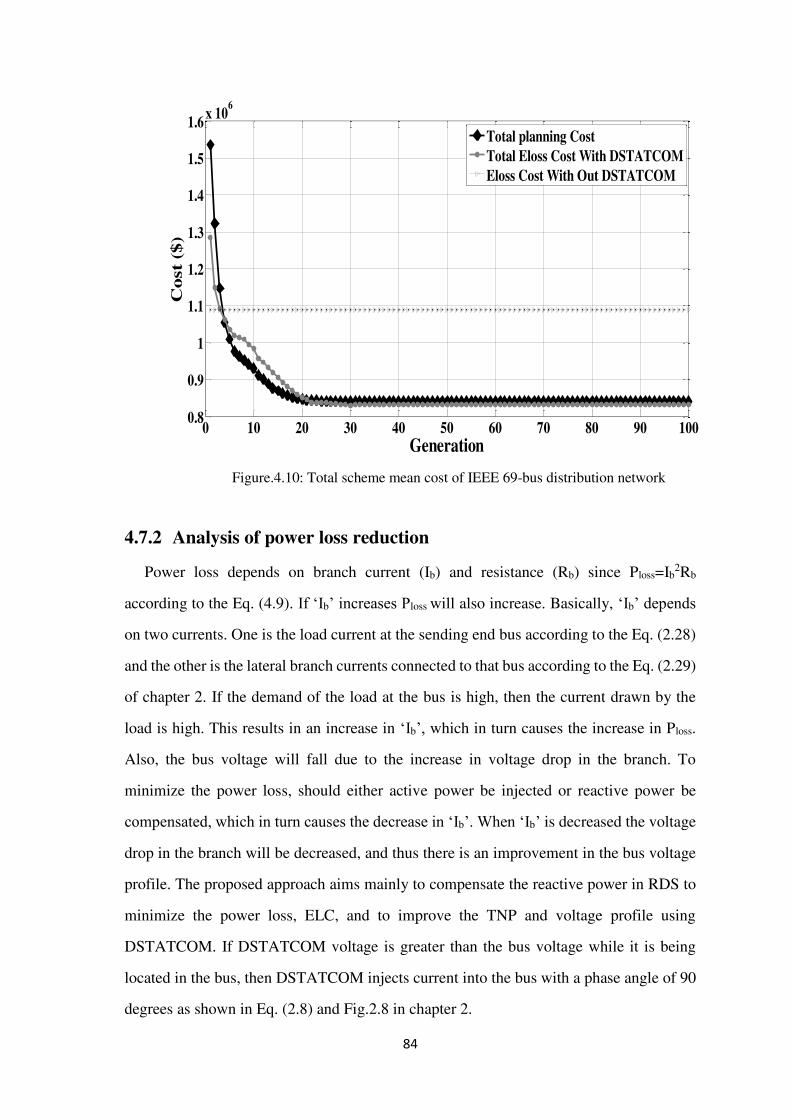
84

Figure.4.10: Total scheme mean cost of IEEE 69-bus distribution network

4.7.2 Analysis of power loss reduction

Power loss depends on branch current (Ib) and resistance (Rb) since Ploss=Ib2Rb

according to the Eq. (4.9). If ‘Ib’ increases Ploss will also increase. Basically, ‘Ib’ depends

on two currents. One is the load current at the sending end bus according to the Eq. (2.28)

and the other is the lateral branch currents connected to that bus according to the Eq. (2.29)

of chapter 2. If the demand of the load at the bus is high, then the current drawn by the

load is high. This results in an increase in ‘Ib’, which in turn causes the increase in Ploss.

Also, the bus voltage will fall due to the increase in voltage drop in the branch. To

minimize the power loss, should either active power be injected or reactive power be

compensated, which in turn causes the decrease in ‘Ib’. When ‘Ib’ is decreased the voltage

drop in the branch will be decreased, and thus there is an improvement in the bus voltage

profile. The proposed approach aims mainly to compensate the reactive power in RDS to

minimize the power loss, ELC, and to improve the TNP and voltage profile using

DSTATCOM. If DSTATCOM voltage is greater than the bus voltage while it is being

located in the bus, then DSTATCOM injects current into the bus with a phase angle of 90

degrees as shown in Eq. (2.8) and Fig.2.8 in chapter 2.

0 10 20 30 40 50 60 70 80 90 1000.8

0.9

1

1.1

1.2

1.3

1.4

1.5

1.6 x 106

Generation

Cos

t ($

)

Total planning CostTotal Eloss Cost With DSTATCOMEloss Cost With Out DSTATCOM

85

Thus, the reactive power demand shall be compensated which minimizes the power

loss and improves the bus voltage eventually. In the case of the 33-bus DN the complex

load power demand (P+jQ) at “bus 30” is higher than the load demand in remaining buses

as shown in the network data given in “Table A” in “Appendix.”

Mainly, the reactive power demand in “bus 30” is higher than all loads connected in

remaining buses. Hence, it is quite natural that the compensation of reactive power highly

occurs at “bus 30”. Thus, in proposed approach, the best location for DSTATCOM

allocation is found to be “bus 30” with the size of 1252.7 kVAr as shown in “Table 4.5.”

Hence, there is certain impact on network power loss when DSTATCOM is located at

buses 3-18, 23 and 26-33. In case of the 69-bus DN, the load power demand at “Bus 61”

is higher than those of the remaining buses as shown in the network data in “Table B” in

“Appendix.” Hence, the best location for DSTATCOM allocation is found to be at “bus

61” with the size of 1312.1 kVAr as shown in “Table 4.5.” There is the certain impact on

network power loss when DSTATCOM is located at buses 6-27 and 51-69 as mentioned

in section 6.1.

Figure.4.11: Power loss at different loads with DSTATCOM at each bus of IEEE 30-bus distribution network

0 5 10 15 20 25 30100

150

200

250

300

350

Bus Number

Pow

er lo

ss (k

W)

Power loss at light load with DSTATCOMPower loss at medium load with DSTATCOMPower loss at peak load with DSTATCOM

86

Figure.4.12: Minimum bus voltage at different loads with DSTATCOM at each bus of IEEE 30-bus distribution network

Figure.4.13: Voltage magnitude at various loads with DSTATCOM at bus 5 of

IEEE 30-bus distribution network

0 5 10 15 20 25 300.85

0.86

0.87

0.88

0.89

0.9

0.91

0.92

0.93

0.94

Bus Number

Min

imu

m v

olta

ge (

p.u

.)

Minimum voltage at light load with DSTATCOMMinimum voltage at medium load with DSTATCOMMinimum voltage at peak load with DSTATCOM

0 5 10 15 20 25 300.86

0.88

0.9

0.92

0.94

0.96

0.98

1

Bus Number

Bu

s V

olta

ge (

p.u

.)

Light load base voltageLigh load voltage with DSTATCOMMedium load base voltageMedium load voltage with DSTATCOMPeak load base voltagePeak load voltage with DSTATCOM

87

Figure.4.14: Size of DSTATCOM at each bus of IEEE 30-busdistribution

network at various loads

Figure.4.15: Power loss at different loads with DSTATCOM at each bus of IEEE 33-bus distribution network

0 5 10 15 20 25 30 350

500

1000

1500

2000

2500

3000

3500

4000

Bus Number

Siz

e (k

VA

r)

Size of DSTATCOM at light loadSize of DSTATCOM at medium loadSize of DSTATCOM at peak load

0 5 10 15 20 25 30 35100

150

200

250

300

350

400

450

Bus Number

Pow

er lo

ss (

kW

)

Power loss at light load with DSTATCOMPower loss at medium load with DSTATCOMPower loss at peak load with DSTATCOM

88

Figure.4.16: Minimum bus voltage at various loads with DSTATCOM at each bus of IEEE 33-bus distribution network

Figure.4.17: Voltage magnitude at various loads with DSTATCOM at bus 30 of IEEE 33-bus distribution network

0 5 10 15 20 25 30 350.87

0.88

0.89

0.9

0.91

0.92

0.93

0.94

Bus Number

Min

imu

m v

olta

ge (

p.u

.)

Minimum voltage at light load with DSTATCOMMinimum voltage at medium load with DSTATCOMMinimum voltage at peak load with DSTATCOM

0 5 10 15 20 25 30 350.86

0.88

0.9

0.92

0.94

0.96

0.98

1

Bus Number

Bu

s V

olta

ge (

p.u

.)

Light load base voltageLigh load voltage with DSTATCOMMedium load base voltageMedium load voltage with DSTATCOMPeak load base voltagePeak load voltage with DSTATCOM

89

Figure.4.18: The size of DSTATCOM at each bus of IEEE 33-bus distribution network at different loads

Figure.4.19: Power loss at different loads with DSTATCOM at each bus of IEEE 69-bus distribution network

0 5 10 15 20 25 30 350

1000

2000

3000

4000

5000

6000

Bus Number

Siz

e (k

VA

r)

Size of DSTATCOM at light loadSize of DSTATCOM at medium loadSize of DSTATCOM at peak load

0 10 20 30 40 50 60 70150

200

250

300

350

400

450

500

550

Bus Number

Pow

er lo

ss (

kW

)

Power loss at light load with DSTATCOMPower loss at medium load with DSTATCOMPower loss at peak load with DSTATCOM

90

Figure.4.20: Minimum bus voltage at various loads with DSTATCOM at each bus of IEEE

69-bus distribution network

Figure.4.21: Voltage magnitude at various loads with DSTATCOM at bus 61 of

IEEE 69-bus distribution network

0 10 20 30 40 50 60 700.86

0.87

0.88

0.89

0.9

0.91

0.92

0.93

0.94

Bus Number

Min

imu

m v

olta

ge (

p.u

.)

Minimum voltage at light load with DSTATCOMMinimum voltage at medium load with DSTATCOMMinimum voltage at peak load with DSTATCOM

0 10 20 30 40 50 60 700.86

0.88

0.9

0.92

0.94

0.96

0.98

1

Bus Number

Bu

s V

olta

ge (

p.u

.)

Light load base voltageLigh load voltage with DSTATCOMMedium load base voltageMedium load voltage with DSTATCOMPeak load base voltagePeak load voltage with DSTATCOM

91

Figure.4.22: Size of DSTATCOM at each bus of IEEE 69-bus distribution

network at different loads

4.7.3 Analysis of planning cost

The total planning cost of the all three bus RDNs are described in this section. Table

4.6 shows the comparative results of the total annual planning cost of the RDNs with

DSTACOM installation. In the approach of [88] to evaluate the TNP/TCS the planning

horizon as shown in Table III is considered only for the evaluation of the DSTATCOM

initial capital investment cost (f21) but not for remaining costs such as energy (power) loss

cost (f1), operational and maintenance cost (f22 and f23) of the DSTATCOM, so to compare

the effectiveness of proposed approach the same scenario is considered along with same

PWF which is used in existed approach [88]. As can be seen, compared with IA, DE offers

an improved optimal solution with its lower F and higher TNP/TCS. It is noteworthy that

the value of F and TNP/TCS are minimized and maximized by 10.5% and 136.18%

respectively in the planning of IEEE 33-bus RDN and 8.49% and 61.25% respectively in

the planning of IEEE 69-bus RDN using DE compared with IA [88] method. As a result

of this approach the TNP/TCS per annum with respect to total energy (power) loss cost

without DSTATCOM are valued to be of the order of 17.91%, 16.93% and 19.63%, in 30,

33 and 69 buses RDNs, respectively.

0 10 20 30 40 50 60 700

1000

2000

3000

4000

5000

6000

Bus Number

Size

(kV

Ar)

Size of DSTATCOM at light loadSize of DSTATCOM at medium loadSize of DSTATCOM at peak load

92

Table 4.8: Comparison of TNP of proposed approach

with the capacitor placement approaches

Test network Approach TNP or

TCS ($)

33 bus

IP [119] 6085

SA [119] 6183

GA [120] 10737

FRCGA 121] 11222

GSA [119] 12389

Proposed 26748

69 bus

IP [119] 9851

DE–PS [127] 12052

GA [120] 12461

CSA [128] 12653

DSA [129] 12712

TLBO [58] 12767

GSA [119] 12837

Proposed 35327

Table 4.9: The solution obtained with proposed de algorithm in 50 run considering

PWF for planning horizon including operational and maintenance cost of DSTATCOM

Test network

Total energy loss cost with DSATCOM (f1)

Total planning cost (F)

Mean ($) Standard deviation Mean ($) Standard

deviation 30-bus 599,630 3.8907 606,646 3.9987

33-bus 833,712 4.0253 847,484 4.7672

69-bus 915,495 6.2860 928,017 6.5719

Table 4.7 shows the economic evaluation of total planning cost result per PH of RDNs

including f22 and f23 considering the PWF as given in Eq. (4.6) and (4.7) in the total

planning horizon. As can be seen in both Table 4.7 and Figs. 4.6 and 4.7 there is an obvious

rise in TNP/TCS by using proposed approach compared to IA approach [88]. The mean

93

curves of F obtained by DE in IEEE 30, 33, and 69-bus RDNs are presented in Figs. 4.8,

4.9 and 4.10 respectively. As shown in Table 4.10 the solution convergence takes place in

DE after 21st, 25th and 28th generation in 30, 33, and 69-bus RDNs respectively which

ascertains that the computational time of proposed algorithm is very faster than the IA,

even after 50th iteration. Also, DE has reached a better answer (i.e. lower F and nearer to

the global optima) compared with IA and GA. The performance comparison of the TNP

with some previous investigations with capacitor allocation has been compared in Table

4.9 and it is observed that the proposed approach with DSTATCOM allocation found

better in achieving higher TNP compared to IP, SA, and TLBO [58], GSA[119], GA[120],

FRCGA[121], DE-PS[127], CSA[128] and DSA[129].

4.7.4 Analysis of ELC

The total ELC of the all three RDS is described in this section. Table 4.6 shows the

comparative results of the total annual ELC of the RDS with DSTATCOM installation

scheme. In the approach of [88] to evaluate TNP the whole PH, is considered only for the

evaluation of the DSTATCOM initial capital investment cost (f21) but not for remaining

costs such as energy (power) loss cost (f1), operational and maintenance cost (f22 and f23)

of the DSTATCOM, so to compare the effectiveness of proposed approach the same

scenario is considered along with same PWF which is used in existed approach [88]. As

can be seen, compared with IA, DEA offers an improved optimal solution with its lower

F and higher TNP.

Table 4.10: Comparison of convergence of mean curve of F

Test network Approach Convergence of F

occurred CPU

Time(s)

30-bus Proposed After 21st generation 175.38

IA [88] -- --

33-bus

Proposed After 25th generation 200.02

IA [88] After 50th generation 21,220

GA [88] After 75th generation 24,157

69-bus

Proposed After 28th generation 789.25

IA [88] After 50th generation 32,305

GA [88] -- 45,588

94

It is noteworthy that the value of F and TNP are minimized and maximized by 10.5%

and 136.18% respectively in the scheme of IEEE 33-bus DN and 8.49% and 61.25%

respectively in the scheme of IEEE 69-bus DN using DEA compared with IA [88] method.

As a result of this approach the TNP per annum with respect to total ELC with

DSTATCOM are valued to be of the order of 17.91%, 16.93%, and 19.63%, in 30, 33 and

69 buses DN, respectively. Similarly, for the total PH of DSTATCOM installation scheme

(30 years), 22.88%, 20.39%, and 22.90% of TNP has been achieved by proposed approach

in 30, 33 and 69 bus system respectively as shown in “Tables 4.7” which is quite profitable

and useful for "DISCOs" (distribution companies).

4.8 Conclusion

This paper presents optimization of total ELC of DS with DSTATCOM allocation. In

this scheme minimization of Ploss, improvement in voltage profile, minimization of ELC

and installation cost of the DSTATCOM and, the maximization of TNP are obtained by

sizing and allocating the DSTATCOM optimally in RDS using DEA. The objective

function is defined by using energy losses and its associated cost after the installation of

DSTATCOM. Forward- backward sweep load flow algorithm is used for the solution of

the network. Simulation results show that the objective function is optimized with

DSTATCOM using DEA. Compared with IA, DEA technique offers minimum power loss,

CPU time, objective function and maximum TNP. The reduction in total ELC after the

installation of DSTATCOM by the proposed approach for the whole PH of DSTATCOM

installation scheme leads to 23.86%, 21.14% and 23.61% in 30, 33 and 69 buses DN,

respectively. TNP as a result of this approach is valued to be of the order of 22.88%,

20.39%, and 22.90%, in 30, 33 and 69 buses DN, respectively. The simulation results in

Table 4.5, and 4.7 of proposed work are found better compared to [88] and [119]. The

voltage at each bus and current in each line are within the permissible boundaries. This is

all about the allocation of single DSTATCOM in RDS. However, the next chapter

investigates and describes what happens to the system power loss and bus voltage if the

reactive power is compensated by the multiple DSTATCOMs and the combination of

DSTATCOM and DG.

95

Appendix:

Tables A and B show the line and bus data of 33 and 69 bus radial distribution systems

under light load condition. Medium load condition is considered as the sum of light load

and 30% of light load. Peak load condition is considered as the sum of light load and 60%

of the light load according to the reference [88]. The three load conditions have been

considered from reference [88] since the simulation results of proposed approach in this

chapter has been compered mainly with the ref [88].

Table A: Data of 33 bus RDS

Bus Line Data Bus Data

Send Receive Line

Resistance (Ω)

Line Reactance

(Ω)

Active Load power (kW)

Reactive Load power (kVAr)

1 2 0.0922 0.0470 100 60 2 3 0.4930 0.2511 90 40 3 4 0.3660 0.1864 120 80 4 5 0.3811 0.1941 60 30 5 6 0.8190 0.7070 60 20 6 7 0.1872 0.6188 200 100 7 8 0.7114 0.2351 200 100 8 9 1.0300 0.7400 60 20 9 10 1.0440 0.7400 60 20

10 11 0.1966 0.0650 45 30 11 12 0.3744 0.1238 60 35 12 13 1.4680 1.1550 60 35 13 14 0.5416 0.7129 120 80 14 15 0.5910 0.5260 60 10 15 16 0.7463 0.5450 60 20 16 17 1.2890 1.7210 60 20 17 18 0.7320 0.5740 90 40 2 19 0.1640 0.1565 90 40

19 20 1.5042 1.3554 90 40 20 21 0.4095 0.4784 90 40 21 22 0.7089 0.9373 90 40 3 23 0.4512 0.3083 90 50

23 24 0.8980 0.7091 420 200 24 25 0.8960 0.7011 420 200 6 26 0.2030 0.1034 60 25

26 27 0.2842 0.1447 60 25 27 28 1.0590 0.9337 60 20 28 29 0.8042 0.7006 120 70 29 30 0.5075 0.2585 200 600 30 31 0.9744 0.9630 150 70 31 32 0.3105 0.3619 210 100 32 33 0.3410 0.5302 60 40

96

Table B: Data of 369 bus RDS

Bus Line Data Bus Data

Send Receive Line

Resistance (Ω)

Line Reactance

(Ω)

Active Load power (kW)

Reactive Load power (kVAr)

1 2 0.0005 0.0012 0 0 2 3 0.0005 0.0012 0 0 3 4 0.0015 0.0036 0 0 4 5 0.0251 0.0294 0 0 5 6 0.366 0.1864 2.6 2.2 6 7 0.3811 0.1941 40.4 30 7 8 0.0922 0.047 75 54 8 9 0.0493 0.0251 30 22 9 10 0.819 0.2707 28 19

10 11 0.1872 0.0691 145 104 11 12 0.7114 0.2351 145 104 12 13 1.03 0.34 8 5.5 13 14 1.044 0.345 8 5.5 14 15 1.058 0.3496 0 0 15 16 0.1966 0.065 45.5 30 16 17 0.3744 0.1238 60 35 17 18 0.0047 0.0016 60 35 18 19 0.3276 0.1083 0 0 19 20 0.2106 0.0696 1 0.6 20 21 0.3416 0.1129 114 81 21 22 0.014 0.0046 5.3 3.5 22 23 0.1591 0.0526 0 0 23 24 0.3463 0.1145 28 20 24 25 0.7488 0.2745 0 0 25 26 0.3089 0.1021 14 10 26 27 0.1732 0.0572 14 10 3 28 0.0044 0.0108 26 18.6

28 29 0.064 0.1565 26 18.6 29 30 0.3978 0.1315 0 0 30 31 0.0702 0.0232 0 0 31 32 0.351 0.116 0 0 32 33 0.839 0.2816 14 10 33 34 1.708 0.5646 19.5 14 34 35 1.474 0.4873 6 4 3 36 0.0044 0.0108 26 18.55

36 37 0.064 0.1565 26 18.55 37 38 0.1053 0.123 0 0 38 39 0.0304 0.0355 24 17 39 40 0.0018 0.0021 24 17 40 41 0.7283 0.8509 1.2 1 41 42 0.31 0.3623 0 0 42 43 0.041 0.0478 6 4.3 43 44 0.0092 0.0116 0 0 44 45 0.1089 0.1373 39.22 26.3 45 46 0.0009 0.0012 39.22 26.3 4 47 0.0034 0.0084 0 0

97

47 48 0.0851 0.2083 79 56.4 48 49 0.2898 0.7091 384.7 274.5 49 50 0.0822 0.2011 384.7 274.5 8 51 0.0928 0.0473 40.5 28.3

51 52 0.3319 0.1114 3.6 2.7 9 53 0.174 0.0886 4.35 3.5

53 54 0.203 0.1034 26.4 19 54 55 0.2842 0.1447 24 17.2 55 56 0.2813 0.1433 0 0 56 57 1.59 0.5337 0 0 57 58 0.7837 0.263 0 0 58 59 0.3042 0.1006 100 72 59 60 0.3861 0.1172 0 0 60 61 0.5075 0.2585 1244 888 61 62 0.0974 0.0496 32 23 62 63 0.145 0.0738 0 0 63 64 0.7105 0.3619 227 162 64 65 1.041 0.5302 59 42 11 66 0.2012 0.0611 18 13 66 67 0.0047 0.0014 18 13 12 68 0.7394 0.2444 28 20 68 69 0.0047 0.0016 28 20

98

Chapter 5

Optimal Phase Angle injection for Reactive Power Compensation of

Distribution Systems with the Allocation of Multiple DSTATCOM and DG

5.1. Introduction

In this chapter, the allocation of optimal phase angle model of multiple distribution

STATCOM (DSTATCOM) and the combination of both DSTATCOM and DG

(distributed generation) in RDS for the optimal reactive power compensation is presented.

The objective function used in this approach is same as that of the objective function used

in chapter 3, which is Eq. (3.1). The optimal location(s), optimal phase angle(s), and

rating(s) for DSTATCOM and DG, are determined based on the best reduction in

minimum power loss of radial distribution systems (RDS). The role of DSTATCOM in

this chapter is injecting reactive power and the role of DG is injecting active power in to

the RDS. Firstly, the impact of multiple DSTATCOM allocation on system power loss and

voltage have been studied. Secondly, the impact of combination of single DSTATCOM

and DG allocation on RDS have been studied.

5.2. Multiple DSTATCOM allocation

In this section, the new modeling of DSTATCOM developed in chapter 2 is allocated

in multiples of single DSTATCOM in RDS to compensate the reactive power. Multiple

DSTATCOMs are suitably incorporated in the forward-backward sweep (FBS) load flow

algorithm in the same manner discussed in chapter 2 so as to determine the line currents,

node voltages and the power loss of RDS. Differential evolution (DE) algorithm is used as

the optimal solution scheme for the optimization of the power loss. The 69-bus RDS is

used to validate the efficacy of the proposed approach. The results demonstrate that the

99

proposed technique is more effective in compensating the reactive power to reduce the

power loss compared to some of the previous approaches.

As discussed in chapter 1.2 the previous studies investigated that the higher reduction

of power loss is possible with simultaneous use of different reactive power compensation

techniques, for example, DSTATCOM allocation along with network reconfiguration, DG

placement with network reconfiguration, DSTATCOM placement for supplying reactive

power to the DG units, a combination of DVR (dynamic voltage restorer) and D-

STATCOM etc. However, there are certain problems with the use of combinatorial devices

and methods. The combination of optimal operation and network reconfiguration of the

distribution system is a complicated problem since the network reconfiguration results in

a change in topology of feeder structure by opening or closing of sectionalizes. Moreover,

the control of DSTATCOM with DG in the distribution systems is complex, and a DVR

is costlier as compared to a DSTATCOM. In view of all these difficulties, it is interesting

to investigate the impact of optimal allocation of multiple DSTATCOM in RDS.

5.2.1. Proposed Solution Strategy Using DE

The parameter values and optimal problem variables for this case are mentioned in

Table. 5.1. A typical string structure is shown in Fig. 5.1 used in this approach. The

dimension of each string is seven in this approach. The first variable NDSTAT in the string

represents the number of DSTATCOMs considered in the string. The DSTATCOM 1,

DSTATCOM 2, and DSTATCOM 3 in the string are represented by the variables n1, n2,

and n3 respectively. The corresponding phase angle variables of DSTATCOMs are

represented by β'n+1,n1, β'

n+1,n1, and β'n+1,n1. The locations for DSTATCOM are engaged in the

same manner of the approach in chapter 3. Multiple DSTATCOMs are allocated one at a

time at all the nodes except the substation node the range of the angle β'n+1 lies in between

0 to 90 degrees. The DEA discussed in chapter 3 is the solution strategy in this approach

to optimize the locations and sizes for the DSTATCOM in RDS in order to optimize the

power loss and voltage profile.

100

Table 5.1: Parameters of DE algorithm

NP D F CR Generations

50 7 0.7 0.8 100

5.2.2. Simulation Results

In this section, the simulation results are presented to show the impact of the allocations

of multiple DSTATCOM in the network in minimizing the power loss. To alleviate the

effectiveness of the proposed approach a 69 bus RDS is considered as the test system. The

data of 69 bus RDS is taken from the ‘appendix B’ in 4th chapter. The active and reactive

power loss of the system before the installation of DSTATCOM(s) are 224.98 kW and

102.1kVAr respectively. The simulation results obtained with the allocation two

DSTATCOMs proposed work have been compared with BFOA approach [130] and

reconfiguration and DSTATCOM allocation scheme [57] in Table 5.2. The Table 5.3

provides the reactive power compensation in RDS using multiple DSTATCOMs i.e.

allocation of three, four, five and six combinations of DSTATCOM in RDS. To simplify

the explanation of the proposed approach in this section has been considered as different

cases operations and each combination is named with a case number as follows:

Case-1: Allocation of two DSTATCOMs

Case-2: Allocation of three DSTATCOMs

Case-3: Allocation of four DSTATCOMs

Case-4: Allocation of five DSTATCOMs

Case-5: Allocation of six DSTATCOMs

Number of DSTATCOMs

Location of DSTATCOMs

Value of β'n+1 corresponding

to the location of DSTATCOM

NDSTAT n1 n2 n3 β'n+1,n1 β'n+1,n2 β'n+1,n3

Figure.5.1: A typical string for DE

101

5.2.2.1. Results of Multiple-DSTATCOM allocation using DE

This section explains the simulation results of DEA based multiple DSTATCOM

approach. The minimum power loss corresponding to the best solution in each generation

with multiple DSTATCOM allocation is shown in Fig. 5.2. The mean power loss of the

population in each generation is shown in Fig. 5.3. The optimal locations and sizes for the

DSTATCOM are given in Table 5.2. The minimum power loss is found to be 146.4kW

with the 31.52° and 42.24° of optimal phase angles injection by the DSTATCOMs at buses

17, 61 respectively. The corresponding rating of DSTATCOM 1, and DSTATCOM 2 are

361.1 kVAr and 1275.1 respectively. Fig. 5.4 represents the voltage profile of the RDS

before and after the allocation of multiple DSTATCOMs i.e. two DSTATCOMs. Before

the installation DSTATCOMs, the minimum voltage of the system is recorded as 0.9092

p. u. and after the installation of multiple DSTATCOMs, it has been improved to 0.9312

p. u. The voltage profile of the systems is improved by 2.41% with the proposed approach.

The voltage profile is the main parameter to maintain properly at each moment in the RDS

since RDS delivers the power to the consumers.

Table 5.2: Comparative results of multiple DSTATCOMs allocation

Parameter Base Case

Ref [57] - DSTATCOM with

reconfiguration (Example-1, Case-4)

Ref [130]

BFOA

Proposed Approach with

two DSTATCOMs (Case-1)

Optimal phase angle (β'

n+1) --

-- -- 31.52°

-- -- 42.24°

Optimal sizes (kVAr) and

locations --

Reconfiguration 480(15) 361.1(17)

2680(61) 1430(61) 1275.1(61)

Total kVAr -- 2680 1910 1636

Power loss (kW) 224.9 137.49 148.0 146.4

% Reduction in power loss -- 38.8 34.1 35.0

Reactive power loss (kVAr) 102.1 128.74 68.7 68.2

% Reduction in reactive power loss -- -26.1 32.7 33.2

Minimum voltage 0.9092 -- -- 0.9312

102

Figure.5.2: Power loss corresponding to the best solution with multiple DSTATCOM

allocation

Figure.5.3: Mean power loss of each generation with multiple DSTATCOM allocation

0 20 40 60 80 100145

150

155

160

165

Generation

Min

imum

Act

ive

Pow

er L

oss (

kW)

0 20 40 60 80 100140

160

180

200

220

Generation

Mea

n A

ctiv

e Po

wer

Los

s (kW

)

103

Figure.5.4: Voltage profile with and without allocation of multiple DSTATCOM

5.2.2.2. Comparative results with some of the previous works

Table 5.2 shows the comparison of power loss with previous methods in reducing the

power loss of 69-bus RDS when the combinatorial devices are allocated to the system. In

the proposed approach the active and reactive power loss of the network are found to be

146.4 kW and 68.2 kVAr when two DSTATCOMs(case-1) are optimally placed in the

system simultaneously in the locations 17, and 61 with 31.52°, and 42.24° of optimal phase

angle injection respectively. The active and reactive power loss are reduced by 35.0% and

33.2% respectively in the proposed approach, whereas, in BFOA approach the active and

reactive power loss are reduced by 34.1% and 32.7% respectively with the placement of

two DSTATCOMs in different locations respectively. In ref [57], 38.8% of power loss

are reduced with DSTATCOM and reconfiguration technique. However, the size of the

DSTATCOM is very high compared to the total optimal size of multiple DSTATCOM in

the proposed approach. Moreover, the reactive power loss are increased by 26.1% (-

26.1%) compared to base case reactive power loss. As discussed in section ‘1.2 in chapter

0 20 40 60 800.9

0.92

0.94

0.96

0.98

1

Bus

Vol

tage

(p.u

.)

Base case voltage

Voltage with Multiple DSTATCOMallocation

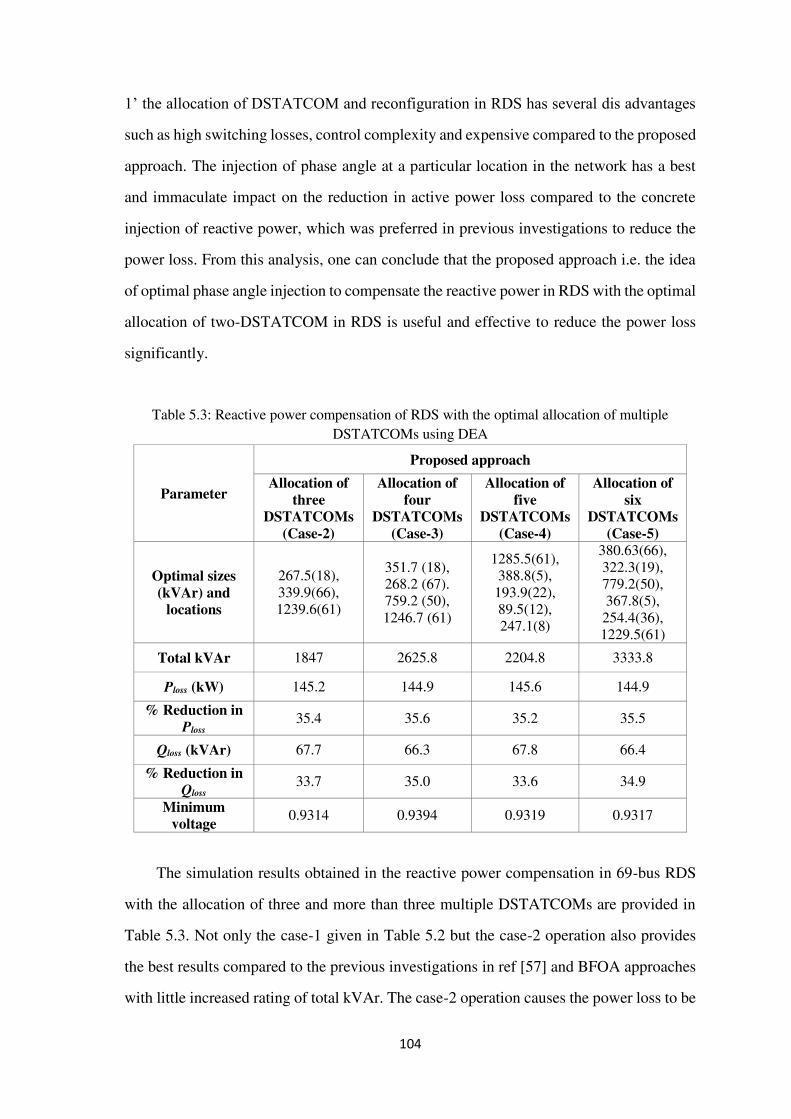
104

1’ the allocation of DSTATCOM and reconfiguration in RDS has several dis advantages

such as high switching losses, control complexity and expensive compared to the proposed

approach. The injection of phase angle at a particular location in the network has a best

and immaculate impact on the reduction in active power loss compared to the concrete

injection of reactive power, which was preferred in previous investigations to reduce the

power loss. From this analysis, one can conclude that the proposed approach i.e. the idea

of optimal phase angle injection to compensate the reactive power in RDS with the optimal

allocation of two-DSTATCOM in RDS is useful and effective to reduce the power loss

significantly.

Table 5.3: Reactive power compensation of RDS with the optimal allocation of multiple DSTATCOMs using DEA

Parameter

Proposed approach Allocation of

three DSTATCOMs

(Case-2)

Allocation of four

DSTATCOMs (Case-3)

Allocation of five

DSTATCOMs (Case-4)

Allocation of six

DSTATCOMs (Case-5)

Optimal sizes (kVAr) and

locations

267.5(18), 339.9(66), 1239.6(61)

351.7 (18), 268.2 (67). 759.2 (50), 1246.7 (61)

1285.5(61), 388.8(5),

193.9(22), 89.5(12), 247.1(8)

380.63(66), 322.3(19), 779.2(50), 367.8(5),

254.4(36), 1229.5(61)

Total kVAr 1847 2625.8 2204.8 3333.8

Ploss (kW) 145.2 144.9 145.6 144.9

% Reduction in Ploss

35.4 35.6 35.2 35.5

Qloss (kVAr) 67.7 66.3 67.8 66.4

% Reduction in Qloss

33.7 35.0 33.6 34.9

Minimum voltage 0.9314 0.9394 0.9319 0.9317

The simulation results obtained in the reactive power compensation in 69-bus RDS

with the allocation of three and more than three multiple DSTATCOMs are provided in

Table 5.3. Not only the case-1 given in Table 5.2 but the case-2 operation also provides

the best results compared to the previous investigations in ref [57] and BFOA approaches

with little increased rating of total kVAr. The case-2 operation causes the power loss to be

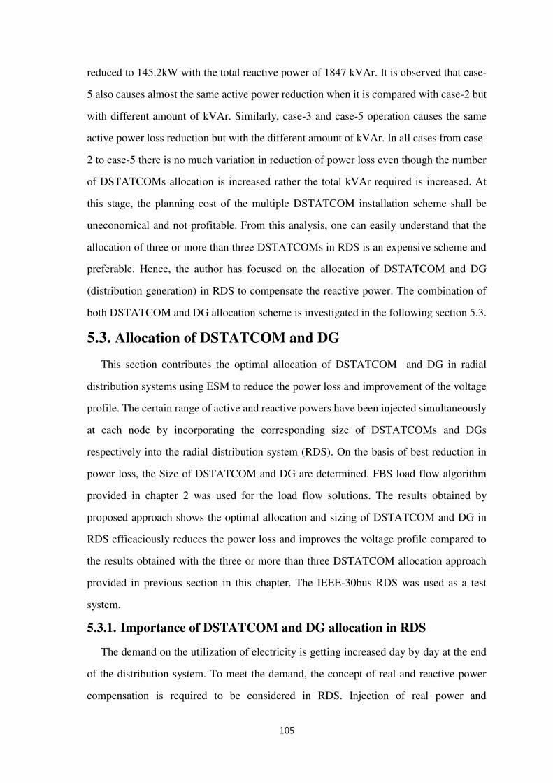
105

reduced to 145.2kW with the total reactive power of 1847 kVAr. It is observed that case-

5 also causes almost the same active power reduction when it is compared with case-2 but

with different amount of kVAr. Similarly, case-3 and case-5 operation causes the same

active power loss reduction but with the different amount of kVAr. In all cases from case-

2 to case-5 there is no much variation in reduction of power loss even though the number

of DSTATCOMs allocation is increased rather the total kVAr required is increased. At

this stage, the planning cost of the multiple DSTATCOM installation scheme shall be

uneconomical and not profitable. From this analysis, one can easily understand that the

allocation of three or more than three DSTATCOMs in RDS is an expensive scheme and

preferable. Hence, the author has focused on the allocation of DSTATCOM and DG

(distribution generation) in RDS to compensate the reactive power. The combination of

both DSTATCOM and DG allocation scheme is investigated in the following section 5.3.

5.3. Allocation of DSTATCOM and DG

This section contributes the optimal allocation of DSTATCOM and DG in radial

distribution systems using ESM to reduce the power loss and improvement of the voltage

profile. The certain range of active and reactive powers have been injected simultaneously

at each node by incorporating the corresponding size of DSTATCOMs and DGs

respectively into the radial distribution system (RDS). On the basis of best reduction in

power loss, the Size of DSTATCOM and DG are determined. FBS load flow algorithm

provided in chapter 2 was used for the load flow solutions. The results obtained by

proposed approach shows the optimal allocation and sizing of DSTATCOM and DG in

RDS efficaciously reduces the power loss and improves the voltage profile compared to

the results obtained with the three or more than three DSTATCOM allocation approach

provided in previous section in this chapter. The IEEE-30bus RDS was used as a test

system.

5.3.1. Importance of DSTATCOM and DG allocation in RDS

The demand on the utilization of electricity is getting increased day by day at the end

of the distribution system. To meet the demand, the concept of real and reactive power

compensation is required to be considered in RDS. Injection of real power and

106

compensation of reactive power in RDS causes the reduction in total power loss and

improvement in the voltage profile [131]. The real power can be generated by using DG,

so DG’s are also called as the small-scale electricity generators that have become more

prevalent in the present day scenario [87]. The allocation of DG in RDS reduces the power

loss and improves the voltage profile thereby providing the energy security, reduction in

the emission of greenhouse gas [116] and the deregulation of electricity market [117]. The

optimal allocation and the sizing of DG to reduce the power loss using analytical method

was proposed in [118]. The authors of [119] and [120] have proposed the optimal

allocation of multiple DG’s for the reduction of power loss and mitigation of the voltage

problems to improve the efficiency of the system thereby achieving cost profit. However,

the main functioning of DG is generating the active power thus behaving like a real power

source but not reactive power compensator [121]. Hence, the proposed approach in this

chapter consider a DG along with DSTATCOM to compensate the reactive power in RDS.

5.3.2. Problem Formulation

A simple distribution system has a line connected between two nodes i, i+1. It is

considered that there is a load connected at each node. The line real and reactive power

loss between two buses i, i+1 can be evaluated by the following Eq. (5.1) and (5.2)

2 2, 1 , 1

2i i i ii i

loss linei

P QP R

v (5.1)

2 2, 1 , 1

2i i i ii i

loss linei

P QQ X

v (5.2)

The real and reactive power was injected at node i/i+1 by the allocation of DG and

DSTATCOM respectively, then the total power loss in the system can be evaluated by the

following Eq. (5.3)

12

1

nwith DG and DSTATCOM

line linelossi

P I R

(5.3)

DGline load DSTATCOMI I I (5.4)

107

', 1

DG DG DSTATCOMDSTATCOM

P jQI

V i i

(5.5)

The % reduction in power loss after the allocation of both DSTATCOM and DG is defined

as “the ratio of power loss after and before the allocation of DSTATCOM and DG” and it

expressed by the Eq. (5.6).

100with DG and DSTATCOM

total lossloss without DG and DSTATCOM

loss

PP

P (5.6)

5.3.3. Integration of DSTATCOM and DG

The sizes of the both DSTATCOM and DG are chosen between the range of 1 to 2000

kW and kVAr respectively per each division of abscissa. At each node both devices are

allocated simultaneously in an incremental mental way using the ESM algorithm provided

in chapter 3, section 3.2.2. At the value of each division of abscissa, there is a certain

change in the power loss of the system. In addition, it is observed that ESM algorithm

found an optimal reduction in the power loss and improvement in voltage profile in RDS

at the end of final iteration with the integration of optimal size of DSTATCOM and DG at

particular nodes. Generally, Distribution systems suffer from high power loss due to high

R/X ratio, so the traditional load flow studies such as Newton-Raphson method, Gauss-

Seidel and fast-decoupled methods cannot be used to find the load flows and voltages in

RDS. There are several load flow techniques have been proposed by researchers for

distributions systems [132-134]. In this approach, forward-backward load flow algorithm

provided in chapter 2 is used for the load flow solutions. Table 5.4 described the algorithm

developed for the allocation of DSTATCOM and DG. Fig. 5.5 shows a generalized flow

chart of forward-backward sweep algorithm integrating the DSTATCOM and DG in ESM

algorithm. In this approach both ESM and FBS, algorithms have considered the injection

of active power also by using DG. Hence, in 7th line of algorithm it can be seen that the

QDG is injected into the active load power of the RDS. So, it is reflected in load current

evaluation.

108

Table.5.4: ESM Algorithm for the allocation of DSTATCOM and DG:

Require: Initialization of accuracy; maxiter; no. of nodes;

Require: Read the bus data and line data

Require: Create dummy matrices mat, V, X, and Rosh with required sizes in zeros/ones

for location=1:n

for cap=1:1:pahse angle or specified maximum limit of QDSTATCOM and QDG rating

for iter=1:maxiter

for j=n:-1:2

Ij=conj (complex(s (j, 1)-QDG, s (j, 2)-QDSTATCOM)/V (1, j));

while (j<=n)

count=0;

if (count==1)

end node = j;

elseif (count==2)

end

break

end

end

if (max (abs (DIF))<=accuracy) %( check convergence)%

break

end

end

P loss /Q loss =0;

for b=1:n-1

Evaluate (P loss /Q loss)

end

Rosh (location, cap) = P loss /Q loss;

end

end

Print size of DSTATCOM; Plot minimum P loss /Q loss and voltage;

109

N

Y

N

Y

Start

Initialize the system parameters and Read the System data

Save the information of radial structure in matrix ‘X’

Construction of matrix ‘Y’ and ‘Z’, which has the information of laterals of radial structure and the values of, branch currents

respectively

Gen=1: iteration

Start the Forward sweep computation’s with the integration of DG and DSTATCOM sizes according to the range of values

Backward sweep computations and, ccalculation of voltage magnitude at all nodes, and real power loss of the system

Convergence condition fulfilled?

Gen=Gen+1

Gen ≤ Gen max

Stop

Figure.5.5: Flow chart of load flow algorithm with ESM

110

5.3.4. Analysis of Simulation Results

To evaluate the proposed work the 11kV, 100MVA, IEEE 30-node RDS has been

considered [135] and [136]. The accuracy of convergence criteria has been considered as

10-3. The simulation results are not compared with any previous investigations since no

work has considered IEEE 30-bus RDS for the allocation of DSTATCOM and DG.

However, the simulation results obtained in this approach say that this approach is useful

to implement practically in DISCOs to compensate the reactive power to improve the

power quality of the customer.

Table 5.5: Results obtained after the allocation of single DSTATCOM or DG

Parameter Operational aspect

Without DSTATCOM

With Single DSTATCOM at node-5

With Single DG at Node-5

Size kVAr -- 1152 --

kW -- -- 1537

Active Power loss (kW) 147.2 101.4 67.14

Reactive Power Loss (kVA) 89.9 59.5 36.7

Minimum node voltage (p.u.) 0.9046 0.9303 0.9546

Active Power loss reduction (%) 00.00 31.01 54.38

Table 5.6: Results obtained with the allocation of DG and DSTATCOM simultaneously

Operational aspect Same location Different location

Node number for DG allocation 5 11

Node number for DSTATCOM allocation 5 5

Size of DG (kW) 1413 815

Size of DSTATCOM (kVAr) 1152 1152

Active power loss(kW) 28.88 46.4

Reactive power loss (kVA) 11.3 22.5

Minimum node voltage(p.u.) 0.9740 0.9548

Active power loss reduction (%) 80.38 68.47

111

5.3.4.1. Power loss reduction

Fig.5.6 shows power loss reduction with the different sizes of DSTATCOM and DG

from 1 to 2000 kW and kVAr respectively at all nodes of RDS. Also from Fig.5.6 it is

clear that the maximum feasible reduction in power loss was achieved, at a particular

location with the certain size of DSTATCOM/DG. As mentioned in Table 5.5 the base

case power loss of the system i.e. 147.2 kW was reduced to 67.14 kW and 101.4 kW when

the 1537 kW size of DG and 1152 kVAr size of DSTATCOM are respectively allocated

at node-5 individually alone.

Figure: 5.6: Variation of power loss with increment of DG size in each node

Table 5.5, and Fig.5.7 show that the allocation of DG causes a better reduction in power

loss and improvement in voltage profile compared to the allocation of DSTATCOM in

RDS. Fig.5.8 describes the various sizes of DSTATCOM and DG corresponding to the

minimum power loss. It is observed that the sizes of DG compared to DSTATCOM are

higher at all times to reduce the power loss when they are allocated in the system

individually alone. Normally, the cost of DG is higher than the DSTATCOM, so it is an

interest to allocate the DSTATCOM and DG together simultaneously in the system so as

to reduce the size and cost of DG to achieve the maximum possible reduction in power

0500

10001500

2000

6080

100120

140160

180200

-1

0

1

DG Size (kW)

Power Loss (kW)

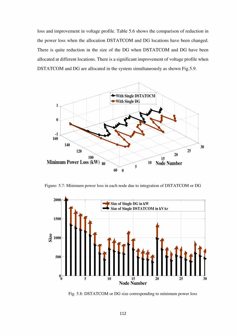
112

loss and improvement in voltage profile. Table 5.6 shows the comparison of reduction in

the power loss when the allocation DSTATCOM and DG locations have been changed.

There is quite reduction in the size of the DG when DSTATCOM and DG have been

allocated at different locations. There is a significant improvement of voltage profile when

DSTATCOM and DG are allocated in the system simultaneously as shown Fig.5.9.

Figure: 5.7: Minimum power loss in each node due to integration of DSTATCOM or DG

Fig. 5.8: DSTATCOM or DG size corresponding to minimum power loss

05

1015

2025

30

6080

100120

140160

-1

0

1

Minimum Power Loss (kW) Node Number

With Single DSTATOCMWith Single DG

0 5 10 15 20 25 300

500

1000

1500

2000

Node Number

Size

Size of Single DG in kWSize of Single DSTATCOM in kVAr

113

Figure.5.9: Voltage magnitude with DSTATCOM and DG at node 5

5.3.4.2.Benefit analysis of the proposed approach

Table 5.5 and 5.6 shows the benefit of proposed approach. 31.01% and 54.38 % power

losses are reduced when single DSTATCOM and DG alone have been respectively

allocated in RDS. When both the devices are allocated simultaneously in RDS at same

location, the 80.53% of power losses are reduced respectively. Also, it is seen in Fig.5.7

the system power losses are affected significantly when the devices are allocated at the

nodes 5, 10, 14 and 20.

5.4. Conclusion

This paper presents the reactive power compensation in RDS by integrating the

multiple-DSTATCOM and the combination of both DSTATCOM and DG in the system.

FBS load flow technique is applied for the calculation of power flow and losses in the

system. The amount of phase angle injection by the DSTATCOM that must be injected

into the system to compensate the reactive power to reduce the power loss is considered

from the modeling of DSTATCOM provided in chapter 3. The 69-bus, and 30-bus RDS

are used as a test systems to illustrate the incorporation of multiple-DSTATCOM and

DSTATCOM and DG combination. DEA provided in chapter 3 is used to optimize the

location and phase angle injection of DSTATCOM to compensate the required amount of

05

1015

2025

30

0.90.92

0.940.96

0.981

-1

0

1

Node NumberVoltage (p.u.)

Base VoltageVoltage With Single DSTATOCMVoltage With Single DSTATOCM and DG

114

reactive power in 69-bus RDS. The ESM algorithm is used to optimize the The optimal

allocation of DSTATCOM and DG to compensate the required amount of reactive power

in IEEE-30 bus RDS. The load flow results in MATLAB shows the impact of Multiple-

DSTATCOM and DSTATCOM and DG to reduce the power loss. Installation of multiple

DSTATCOMs leads maximum of 35.6% of power loss reduction in this approach. The

problem formulated for the allocation of DSTATCOM and DG is integrated into the

forward-Backward sweep load flow algorithm to study the impact of the allocation of these

devices. The ESM algorithm is used to determine the best size and location of

DSTATCOM and DG to achieve the best possible reduction in power loss. The

combination of both DSTATCOM and DG allocation in IEEE 30-bus RDS minimizes the

80.53% of system active power loss, which provides great benefit to the utility customers

and consumers.

115

Chapter 6

Conclusion and Future Scope

6.1. Conclusion

This thesis is focused on the optimal planning of Distribution STATCOM in

distribution systems to optimize the total energy loss cost and the total net profit (total

economic cost benefit) per annum and planning horizon. These objectives are achieved

by compensating the reactive power in DS by allocating the DSTATCOM optimally.

The new phase angle model of DSTATCOM is devolved to determine the rating of

DSTATCOM to generate reactive power. The reactive power is compensated by

injecting the phase angle.

The forward-backward sweep load flow algorithm is developed to suitably incorporate

the DSTATCOM in distribution systems and to evaluate the power loss, line current

and node voltages of distribution systems.

A new objective function is formulated to evaluate the objectives of the thesis such as

optimization of power loss, energy loss cost, total net profit and voltage profile.

The PWF and PH have been considered in objective function since the planning of

DSTATCOM in distribution system occurs once for planning era.

The ESM and DEA optimizing techniques are used to find the optimal size and

location(s) of DSTATCOM. The soft constraints method has been implemented in

optimization technique to avoid the abnormal conditions in the operation of

distribution system. Line currents, node voltages and the size of the DSTATCOM are

maintained in safe limits using soft constraints technique.

The multiple DSTATCOMs and the combination of both DSTATCOM and DG have

also been allocated optimally to compensate the reactive power in the DS so that the

best approach to compensate the reactive power in DS can be opted.

To validate the proposed approach 30, 33, and 69 bus RDNs are considered as test

systems. The results performance of proposed approach are compared with several

116

previous investigations and it is observed that the proposed approach is better and

profitable to implement practically in DISCO’s.

6.2. Future Scope

Research work presented in this thesis can be extended in following dimensions in future.

1) Control strategy of single and multiple DSTATCOM(s) can be investigated to

control the DSTATCOM according to the requirements of the distribution systems

to mitigate the power quality issues.

2) Multi objective fuzzy based Pareto optimization technique can be developed to

allocate DSTATCOM in distribution systems to mitigate high power loss,

harmonics, voltage stability and linelodabilty at different load conditions etc.

3) The combinatorial allocation of DSTATCOM and DVR in distribution systems can

fulfill the purpose of both shunt and series compensations to mitigate power quality

issues.

4) Modeling of multiple DSTATCOM

117

References

[1] S.W. Blume, “Electric power system basics for the nonelectrical professional.” John

Wiley & Sons, 2016.

[2] Y. Del Valle, G. K. Venayagamoorthy, S. Mohagheghi, J. C. Hernandez, and R. G.

Harley, “Particle swarm optimization: basic concepts, variants and applications in

power systems.” IEEE Transactions on evolutionary computation. vol.12, no.2, pp:

171-195, 2008.

[3] A. Demirbas, “Biodiesel: a realistic fuel alternative for diesel engines.” Springer

Science & Business Media, 2007.

[4] I. Hore-Lacy, “Nuclear electricity.” Uranium Information Centre, Ltd., GPO Box

1649N, Melbourne 3001, Australia. 1999.

[5] I. Krikidis, N. Devroye, and J. S. Thompson, “Stability analysis for cognitive radio

with multi-access primary transmission.” IEEE Transactions on Wireless

Communications., vol.9, no.1, 2010.

[6] J. Maeng, P. V. Tischler, and B. Clements, “U.S. Patent No. 5,991,277.

Washington.” DC: U.S. Patent and Trademark Office. 1999.

[7] E. H. Shin, and D. Kim, “Time and power allocation for collaborative primary-

secondary transmission using superposition coding.” IEEE Communications

Letters, vol.15, no.2, pp: 196-198, 2011

[8] M. Liserre, T. Sauter, and J. Y. Hung, “Future energy systems: Integrating renewable

energy sources into the smart power grid through industrial electronics.” IEEE

industrial electronics magazine. vol.4, no.1, pp: 18-37, 2010.

[9] P. Kundur, N. J. Balu, and M. G. Lauby, “Power system stability and control”. New

York: McGraw-hill., vol.7, 1994.

[10] S. Nordström, E. Birke, and L. Gustavsson, “Reproductive hazards among workers

at high voltage substations.” Bio electromagnetics. vol.4, no.1, pp: 91-101, 1983.

[11] M. Hikita, H. Yamashita, T. Hoshino, T. Kato, N. Hayakawa, T. Ueda, and H.

Okubo, “Electromagnetic noise spectrum caused by partial discharge in air at high

118

voltage substations.” IEEE transactions on power delivery. vol.13, no. 2 pp: 434-

439, 1998.

[12] M. Kezunovic, P. Spasojevic, C. W. Fromen, and D. R. Sevcik. “An expert system

for transmission substation event analysis.” IEEE Transactions on Power

Delivery., vol.8, no. 4, 1942-1949, 1993

[13] N. D. Sadanandan, M. E. Needham, D. W. Hilson, K. W. Morris, and Musoke

Sendaula. “Impact assessment of wind generation on the operations of a power

system.” IEEE transactions on power apparatus and systems, vol. 9, pp: 2905-2911,

1983.

[14] Filimonov. Nikolaevich, Kegeles. Alexei, Borisovich. Mark and Malkin Pavel

Aronovich. “Converter substation for direct current power transmission.” U.S.

Patent 3,530,362, issued September 22, 1970.

[15] M. S. Grover and R. Billinton. “A computerized approach to substation and

switching station reliability evaluation.” IEEE Transactions on Power Apparatus

and Systems, vol.5, pp: 1488-1497, 1974.

[16] T.H. Chen and H.Y. Kuo. “Network modelling of traction substation transformers

for studying unbalance effects.” IEE Proceedings-Generation, Transmission and

Distribution., vol.142, no.2, pp:103-108, 1995

[17] A.J. Wood and B.F. Wollenberg. “Power generation, operation, and control.” John

Wiley & Sons. 2012

[18] S. Stoft, “Power system economics.” Journal of Energy Literature., vol.8, pp.94-99,

2002.

[19] M.L. Markus and J. Pfeffer. “Power and the design and implementation of

accounting and control systems.” Accounting, Organizations and Society, vol.8,

no.2-3, pp.205-218, 1983.

[20] L.K. Kirchmayer, “Economic operation of power systems.” John Wiley & Sons,

1958.

[21] R.D. Zimmerman, C.E. Murillo-Sánchez, and R.J. Thomas. “MATPOWER: Steady-

state operations, planning, and analysis tools for power systems research and

education.” IEEE Transactions on power systems, vol.26, no.1, pp: 12-19, 2011.

119

[22] F.F. Wu, K. Moslehi, and A. Bose, “Power system control centers: Past, present, and

future.” Proceedings of the IEEE, vol.93, no.11, pp.1890-1908, 2005.

[23] D.R. Patrick, and S.W. Fardo, “Electrical Distribution Systems.” The Fairmont

Press, Inc, 2009.

[24] S. Favuzza, G. Graditi, M.G. Ippolito, and E.R. Sanseverino, “Optimal electrical

distribution systems reinforcement planning using gas micro turbines by dynamic

ant colony search algorithm.” IEEE Transactions on Power Systems., vol.22, no.2,

pp.580-587, 2007

[25] J.Z. Zhu, “Optimal reconfiguration of electrical distribution network using the

refined genetic algorithm.” Electric Power Systems Research, vol.62, no.1, pp.37-

42, 2002.

[26] A.G. Ter-Gazarian, and N. Kagan. “Design model for electrical distribution systems

considering renewable, conventional and energy storage units.’ In IEE Proceedings

C (Generation, Transmission and Distribution), Vol.139, No.6, pp. 499-504, 1992.

[27] R.A. Walling, R. Saint, R.C. Dugan, J. Burke, and L.A. Kojovic, “Summary of

distributed resources impact on power delivery systems.” IEEE Transactions on

power delivery, vol.23, no.3, pp: 1636-1644, 2008.

[28] W.H. Kersting, “Radial distribution test feeders.” IEEE Transactions on Power

Systems, vol.6, no.3, pp.975-985, 1991.

[29] N.G. Hingorani, “Introducing custom power”. IEEE spectrum, vol.32, no.6, pp.41-

48, 1995.

[30] A.A. Mazi, B.F. Wollenberg and M.H. Hesse. “Corrective control of power system

flows by line and bus-bar switching.” IEEE Transactions on Power Systems, vol.1,

no.3, pp.258-264, 1986.

[31] M.T. Glinkowski, M.R. Gutierrez, and D. Braun, “Voltage escalation and reignition

behavior of vacuum generator circuit breakers during load shedding.” IEEE

Transactions on Power Delivery, vol.12, no.1, pp.219-226, 1997.

[32] T. Gönen, “Electric power distribution system engineering.” McGraw-Hill College,

1986.

120

[33] L. Xu, and M.Y. Chow, “A classification approach for power distribution systems

fault cause identification.” IEEE Transactions on Power Systems, vol.21, no.1,

pp.53-60, 2006.

[34] A. Mutanen, M. Ruska, S. Repo, and P. Jarventausta, “Customer classification and

load profiling method for distribution systems.” IEEE Transactions on Power

Delivery, vol.26, no.3, pp.1755-1763, 2011.

[35] A.F. Naiem, Y. Hegazy, A.Y. Abdelaziz, and M.A. Elsharkawy. “A classification

technique for recloser-fuse coordination in distribution systems with distributed

generation.” IEEE Transactions on Power Delivery, vol.27, no.1, pp.176-185, 2012.

[36] D.J. Hammerstrom, “AC versus DC distribution systemsdid we get it right.”

In Power Engineering Society General Meeting, IEEE, pp. 1-5, June. 2007,

[37] R.E. Brown, S. Gupta, R.D. Christie, S.S. Venkata, and R. Fletcher, “Automated

primary distribution system design: reliability and cost optimization.” IEEE

Transactions on Power Delivery, vol.12, no.2, pp.1017-1022, 1997.

[38] E.C. Senger, G. Manassero, C. Goldemberg, and E.L. Pellini, “Automated fault

location system for primary distribution networks.” IEEE Transactions on Power

Delivery, vol.20, no.2, pp.1332-1340, 2005.

[39] P.C. Paiva, H.M. Khodr, J.A. Domínguez-Navarro, J.M. Yusta, and A.J. Urdaneta,

‘Integral planning of primary-secondary distribution systems using mixed integer

linear programming.’ IEEE Transactions on Power systems, vol.20, no.2, pp.1134-

1143, 2005

[40] A.M. Cossi, R. Romero, and, J.R.S. Mantovani, “Planning of secondary distribution

circuits through evolutionary algorithms.” IEEE Transactions on power

delivery, vol.20, no.1, pp.205-213, 2005.

[41] H. Kakigano, Y. Miura, and T. Ise, “Distribution voltage control for dc microgrids

using fuzzy control and gain-scheduling technique.” IEEE transactions on power

electronics, vol.28, no.5, pp.2246-2258, 2013.

[42] H. Kakigano, Y. Miura, and T. Ise, “Low-voltage bipolar-type DC microgrid for

super high quality distribution.” IEEE transactions on power electronics, vol.25,

no.12, pp.3066-3075, 2010.

121

[43] R.A. Jabr, “Radial distribution load flow using conic programming.” IEEE

transactions on power systems, vol.21, no.3, pp.1458-1459, 2006.

[44] C.S. Cheng and D. Shirmohammadi. “A three-phase power flow method for real-

time distribution system analysis.” IEEE Transactions on Power Systems, vol.10,

no.2, pp.671-679, 1995.

[45] P. Linares. “Multiple criteria decision making and risk analysis as risk management

tools for power systems planning.” IEEE Transactions on Power Systems, vol.17,

no.3, pp.895-900, 2002.

[46] Wu, Vancouver, Q.H. and J.T. Ma, “Power system optimal reactive power dispatch

using evolutionary programming.” IEEE Transactions on power systems, vol.10,

no.3, pp.1243-1249, 1995.

[47] D.J. Gotham, and G.T. Heydt, “Power flow control and power flow studies for

systems with FACTS devices. IEEE Transactions on power systems, vol.13, no.1,

pp.60-65, 1998.

[48] F. Blaabjerg, R. Teodorescu, M. Liserre, and A.V. Timbus, “Overview of control

and grid synchronization for distributed power generation systems.” IEEE

Transactions on industrial electronics, vol.53, no.5, pp.1398-1409, 2006.

[49] F. Katiraei, R. Iravani, N. Hatziargyriou, and A. Dimeas, “Microgrids

management.” IEEE power and energy magazine, vol.6, no.3, 2008.

[50] J. Sanam, A.K. Panda, and S. Ganguly, “Optimal Phase Angle Injection for Reactive

Power Compensation of Distribution Systems with the Allocation of Multiple

Distribution STATCOM”. Arabian Journal for Science and Engineering, pp.1-9,

2016.

[51] J. Sanam, and S. Ganguly, “Impact of distribution STATCOM allocation on radial

distribution networks.” In Energy, Power and Environment: Towards Sustainable

Growth (ICEPE), 2015 International Conference on (pp. 1-6), June 2015.

[52] P.Kumar, and S. Singh, “Energy efficiency performance of reconfigured radial

networks with reactive power injection.” IEEE 6th India International Conference

in Power Electronics (IICPE), pp.1-6, December 2014.

122

[53] A. T. Davda, B. R. Parekh, and M. D. Desai “Reduction of losses and improvement

in voltage profile for a 2.8 MVA distribution network with Dispersed Generation,”

IEEE International Conference on Power System Technology (POWERCON), pp.1-

5, October 2012.

[54] S. M. Kannan, and S. Slochanal, “Fuzzy logic based optimal capacitor placement on

radial distribution feeders,” IEEE Power India Joint International Conference on

Power System Technology (POWERCON), pp.1-6), October 2008.

[55] P. Raja, M. P. Selvan, and N. Kumaresan, “Enhancement of voltage stability margin

in the radial distribution system with squirrel cage induction generator based

distributed generators,” IET Generation, Transmission & Distribution, vol.7, no.8,

pp.898-906, 2013.

[56] J. Sanam, S. Ganguly, and A.K. Panda, “Placement of DSTATCOM in radial

distribution systems for the compensation of reactive power.” In Innovative Smart

Grid Technologies-Asia (ISGT ASIA), 2015 IEEE, pp.1-6. November 2015.

[57] S.Jazebi, S. H. Hosseinian, and B. Vahidi, “DSTATCOM allocation in distribution

networks considering reconfiguration using differential evolution algorithm.”

Energy Conversion and Management, vol.52, no.7, pp: 2777-2783, 2011.

[58] S.Sultana, and P. K.Roy, “Optimal capacitor placement in radial distribution systems

using teaching learning-based optimization,” International Journal of Electrical

Power & Energy Systems., vol.54, pp.387-398, 2014.

[59] P.S.Georgilakis, and N.D.Hatziargyriou, “A review of power distribution planning

in the modern power systems era: Models, methods and future research,” Electric

Power Systems Research., vol.121, pp.89-100, 2015.

[60] J. Vuletić, and M. Todorovski, “Optimal capacitor placement in radial distribution

systems using clustering based optimization,” International Journal of Electrical

Power & Energy Systems., vol.62, pp.229-236, 2014.

[61] F. M.Dias, B.Canizes, H.Khodr, and M. Cordeiro, “Distribution networks planning

using decomposition optimization technique,” Generation, Transmission &

Distribution, IET, vol.9, no.12, pp.1409-1420, 2015.

123

[62] C. J. Bridenbaugh, D. A. DiMascio, and R. D.Aquila, “Voltage control improvement

through capacitor and transformer tap optimization,” IEEE Transactions on Power

Systems., vol.7, no.1, pp.222-227, 1992.

[63] Gu, Zhenghui, and D. Tom Rizy, “Neural networks for combined control of capacitor

banks and voltage regulators in distribution systems,” IEEE Transactions on Power

Delivery., vol.11, no.4, pp.1921-1928, 1996.

[64] W. El-Khattam, Y. G. Hegazy, and M. M. A. Salama, “An integrated distributed

generation optimization model for distribution system planning,” IEEE Transactions

on Power Systems., vol.20, no.2, pp.1158-1165,2005.

[65] I. Hussain, and A. K. Roy, “Optimal distributed generation allocation in distribution

systems employing modified artificial bee colony algorithm to reduce losses and

improve voltage profile,” IEEE International Conference on Advances in

Engineering, Science and Management (ICAESM), pp.565-570, March 2012.

[66] D. Das, “Optimal placement of capacitors in radial distribution system using a

Fuzzy-GA method,” International Journal of Electrical Power & Energy Systems.,

vol.30, no. 6, pp. 361-367, 2008.

[67] Xu, Yan, Z.Y.Dong, K.P.Wong, L.Evan, and Y. Benjamin, “Optimal capacitor

placement to distribution transformers for power loss reduction in radial distribution

systems,” IEEE Transactions on Power Systems., vol.28, no.4, pp.1-8, Nov.2013.

[68] T. M. Khalil, and A. V. Gorpinich, “Optimal conductor selection and capacitor

placement for loss reduction of radial distribution systems by selective particle

swarm optimization,” In Computer Engineering & Systems (ICCES) Seventh IEEE

International Conference., pp. 215-220, Nov.2012.

[69] D. Arcanjo, J.Pereira, E .Oliveira, W .Peres, L .De. Oliveira, and I.Da.S.Junior,

“Cuckoo search optimization technique applied to capacitor placement on

distribution system problem.” IEEE/IAS international conference on industry

applications (INDUSCON), pp: 1–6, 2012.

[70] S. M. S.Hussain, and M. Subbaramiah, “An analytical approach for optimal location

of DSTATCOM in the radial distribution system,” Energy-Efficient Technologies for

Sustainability (ICEETS), International Conference on IEEE. , pp.1365-1369, 2013.

124

[71] A.Mount, S.Fahad, and M. E. El-Hawary, “Optimal distributed generation allocation

and sizing in distribution systems via artificial bee colony algorithm,” IEEE Trans.

Power Del., vol.26, no. 4, pp.2090-2101, 2011.

[72] D.Q. Hung, N. Mithulananthan, and R. C. Bansal, “An optimal investment planning

framework for multiple distributed generation units in industrial distribution

systems,” Applied Energy., vol.124, pp.62-72, 2014.

[73] T. Niknam, S. I. Taheri, J. Aghaei, S. Tabatabaei, and M. Nayeripour, “A modified

honey bee mating optimization algorithm for multiobjective placement of renewable

energy resources,” Applied Energy., vol.88, no.12, pp.4817-4830, 2011.

[74] A. Soroudi, M. Ehsan, and H. Zareipour, “A practical eco-environmental distribution

network planning model including fuel cells and non-renewable distributed energy

resources,” Renewable Energy., vol.36, no.1, pp.179–188, 2011.

[75] S. Kucuksari, A.M. Khaleghi, M. Hamidi, Y. Zhang, F. Szidarovszky, G. Bayraksan,

and Y. J. Son, “An Integrated GIS, optimization and simulation framework for

optimal PV size and location in campus area environments,” Applied Energy.,

vol.113, pp.1601-1613, 2014.

[76] D.Q. Hung, and N. Mithulananthan, “Multiple distributed generator placement in

primary distribution networks for loss reduction,” IEEE Transactions on Industrial

Electronics., vol.60, no. 4, pp.1700-1708, 2013.

[77] P. S. Georgilakis, and N.D. Hatziargyriou, “Optimal distributed generation

placement in power distribution networks: Models, methods, and future research,”

IEEE Trans. Power Syst., vol.28, no.3, pp.3420-3428, 2013.

[78] W. Li, G. Joos, and J. Belanger, “Real-time simulation of a wind turbine generator

coupled with a battery supercapacitor energy storage system,” IEEE Trans. Ind.

Electron., vol.57, no.4, pp. 1137–1145, Apr. 2010.

[79] A. Pigazo, M. Liserre, R. A. Mastromauro, V. M. Moreno, and A. Dell’Aquila,

“Wavelet-based islanding detection in grid-connected PV systems,” IEEE Trans.

Ind. Electron., vol.56, no.11, p.4445–4455, Nov. 2009.

[80] M. Farhoodnea, A. Mohamed, H. Shareef, and H. Zayandehroodi, “A

Comprehensive Review of Optimization Techniques Applied for Placement and

125

Sizing of Custom Power Devices in Distribution Networks,” Przegląd

Elektrotechniczny., vol. 88, pp.261-265, 2012.

[81] S.Ganguly, “Unified power quality conditioner allocation for reactive power

compensation of radial distribution networks,” IET Generation, Transmission &

Distribution., vol.8, no.8, pp.1418-1429, 2014.

[82] S.Ganguly, “Impact of Unified Power-Quality Conditioner Allocation on Line

Loading, Losses and Voltage Stability of Radial Distribution Systems,” IEEE

Transactions Power Delivery., vol.29, no.4, pp.1859-1867, May 2014.

[83] S.Ganguly, “Multi-Objective Planning for Reactive Power Compensation of Radial

Distribution Networks with Unified Power Quality Conditioner Allocation Using

Particle Swarm Optimization,” IEEE Transactions on Power Systems., vol.29, no.4,

pp.1801-1810, dec.2013.

[84] J.Dixon, M.Luis, J.Rodriguez, and D. Ricardo, “Reactive power compensation

technologies: State-of-the-art review,” Proceedings of the IEEE. , vol.93, no. 12,

pp.2144-2164, 2005.

[85] S. Devi, and M. Geethanjali, “Optimal location and sizing of Distribution Static

Synchronous Series Compensator using Particle Swarm Optimization.”

International Journal of Electrical Power & Energy Systems., vol.62, pp. 646-653,

2014.

[86] M. A. Eldery, E. F. El-Saadany, and M. M. A. Salama, “Effect of distributed

generator on the allocation D-STATCOM in distribution network,” In Power

Engineering Society IEEE General Meeting, pp. 2360-2364, 2005.

[87] S.Devi and M. Geethanjali, “Optimal location and sizing determination of

Distributed Generation and DSTATCOM using Particle Swarm Optimization

algorithm,” International Journal of Electrical Power & Energy Systems., Vol.62,

pp.562-570, 2014.

[88] S. A. Taher and S. A. Afsari, “Optimal location and sizing of DSTATCOM in

distribution systems by immune algorithm,” International Journal of Electrical

Power & Energy Systems., vol.60, pp.34-44, 2014.

126

[89] S.P. Gawande, N.A. Kubde, M.S.Joshi and B.S.Sudame, “Reactive Power

Compensation of Wind Energy Distribution System using Distribution Static

Compensator (DSTATCOM).” IEEE International Conference. , pp. 2160-3162,

2012.

[90] M. H. Haque, “Compensation of distribution system voltage sag by DVR and D-

STATCOM,” Power Tech Proceedings, IEEE Porto., vol.1, 2001.

[91] J. Sanam, S. Ganguly, A.K. Panda, and D. Panigrahy, “Forecasting of AELC and

TESC of distribution systems with the optimal allocation of DSTATCOM.” In

Innovative Smart Grid Technologies-Asia (ISGT-Asia), IEEE, pp. 1100-1103,

November 2016.

[92] MN. Mojdehi, A. Kazemi, and M. Barati, “Network operation and reconfiguration

to maximize social welfare with distributed generations,” In IEEE International

Conference EUROCON. , pp.552–557, 2009.

[93] M. Hosseini, H. A. Shayanfar, and M. Fotuhi-Firuzabad, “Modeling of D-

STATCOM in distribution systems load flow,” journal of Zhejiang university

SCIENCE A., vol.8, no.10, pp.1532-1542, 2007.

[94] A. Jain, A.R. Gupta, and A. Kumar, “An efficient method for D-STATCOM

placement in the radial distribution system,” IEEE 6th India International

Conference in Power Electronics (IICPE), pp.1-6, December 2014.

[95] S. Joseph, S. Ganguly, A. K. Panda. “Distribution STATCOM with optimal phase

angle injection model for reactive power compensation of radial distribution

networks.” Int J Numer Model, https://doi.org/10.1002/jnm.2240, 2017.

[96] S. Joseph, A. K. Panda, and S. Ganguly “Optimization of Energy Loss Cost of

Distribution Networks with the Optimal Placement and Sizing of DSTATCOM

Using Differential Evolution Algorithm.” Arabian Journal for Science and

Engineering, (201t): DOI: 10.1007/s13369-017-2518-y, 2017.

[97] S. Singh and T. Ghose, “Improved radial load flow method,” International Journal

of Electrical Power & Energy Systems., vol.44, no.1, pp.721-727, 2013.

[98] S. Das, and P. N. Suganthan, “Differential evolution: A survey of the state-of-the-

art.” IEEE Trans. Evolutionary Computation., vol.15, no.1, pp: 4-31, 2011.

127

[99] M. Varadarajan, and K. S. Swarup, “Differential evolutionary algorithm for optimal

reactive power dispatch.” International Journal of Electrical Power & Energy

Systems., vol.30, no.8, pp: 435-441, 2008.

[100] J.P. Chiou, C.F. Chang, and C.T. Su, “Ant direction hybrid differential evolution for

solving large capacitor placement problems,” IEEE Trans. Power Syst., vol.19, no.4,

pp.1794–1800, Nov.2004.

[101] M.R. Haghifam, and O.P. Malik, “Genetic algorithm-based approach for fixed and

switchable capacitors placement in distribution systems with uncertainty and time

varying loads,” IET Gen. Trans. Dist., vol.1, pp. 244–252, 2007.

[102] M. H. Moradi, A. Zeinalzadeh, Y. Mohammadi, and, M. Abedini “An efficient

hybrid method for solving the optimal sitting and sizing problem of DG and shunt

capacitor banks simultaneously based on imperialist competitive algorithm and

genetic algorithm,” International Journal of Electrical Power & Energy Systems.,

vol.54, pp.101-111,2014.

[103] M. H. Moradi, and M. Abedini, “A combination of genetic algorithm and particle

swarm optimization for optimal DG location and sizing in distribution systems,”

International Journal of Electrical Power & Energy Systems., vol.34, no.1, pp.66-

74, 2012.

[104] M.K. Mishra, A.Ghosh, and A. Joshi, “Operation of a DSTATCOM in voltage

control mode.” IEEE transactions on power delivery, vol.18, no.1, pp.258-264.

2003.

[105] H. Buch, R.D. Bhagiya, B.A. Shah, and B. Suthar, December. “Voltage profile

management in restructured power system using STATCOM.” In Engineering

(NUiCONE), 2011 Nirma University International Conference on IEEE, pp.1-7,

2011.

[106] M.A. Kamarposhti, and M. Alinezhad, “Comparison of SVC and STATCOM in

static voltage stability margin enhancement.” system, vol.9, p.1, 2010.

[107] D.M. Lee, T.G. Habetler, R.G. Harley, T.L. Keister, and J.R. Rostron, “A voltage

sag supporter utilizing a PWM-switched autotransformer.” IEEE transactions on

power electronics, vol.22, no.2, pp.626-635, 2007.

128

[108] M. Hosseini, and H.A. Shayanfar, “Regular paper modeling of Series and Shunt

Distribution FACTS Devices in Distribution Systems Load Flow.” J. Electrical

Systems, vol. 4, no.4, pp.1-12, 2008.

[109] M.Z. Coban, and R.M. Mersereau, “A fast exhaustive search algorithm for rate-

constrained motion estimation.” IEEE Transactions on Image Processing, vol.7,

no.5, pp.769-773, 1998.

[110] G. Coxson, and J. Russo, “Efficient exhaustive search for optimal-peak-sidelobe

binary codes.” IEEE Transactions on Aerospace and Electronic Systems, vol.41,

no.1, pp.302-308, 2005.

[111] S.M. Sajjadi, M.R. Haghifam, and J. Salehi, “Simultaneous placement of distributed

generation and capacitors in distribution networks considering voltage stability

index,” International Journal of Electrical Power & Energy Systems., vol.46,

pp.366-375, 2013.

[112] E. Naderi, H. Seifi, and M.S.Sepasian, “A dynamic approach for distribution system

planning considering distributed generation,” IEEE Transactions on Power

Delivery., vol.27, no.3, pp.1313-1322, 2012.

[113] M. Ramalinga Raju, K.V.S. Ramachandra Murthy, and K. Ravindra, “Direct search

algorithm for capacitive compensation in radial distribution systems,” International

Journal of Electrical Power & Energy Systems., vol.42, no.1, pp.24-30, 2012.

[114] S. Sundhararajan, and A. Pahwa, “Optimal selection of capacitors for radial

distribution systems using a genetic algorithm,” IEEE Transactions on Power

Systems., vol.9, no.3, pp.1499-1507, 1994.

[115] D. Zou, H. Liu, L. Gao, and S. Li, “A novel modified differential evolution algorithm

for constrained optimization problems.” Computers & Mathematics with

Applications, vol. 61, no.6, pp.1608-1623, 2011

[116] M. Saravanan, S. Mary Raja Slochanal, P. Venkatesh, and J. Prince Stephen

Abraham. “Application of particle swarm optimization technique for optimal

location of FACTS devices considering cost of installation and system loadability.”

Electr. Power Sys. Research, vol.77, no.3, pp: 276-283, 2007.

129

[117] J. S. Savier, and D. Das, “Energy loss allocation in radial distribution systems: A

comparison of practical algorithms,” IEEE Transactions on Power Delivery., vol.24,

no.1, pp.260-267, 2009.

[118] P.H. Jeynes, “Present Worth, or the Time Cost of Money, as a Factor in the Economic

Comparison of Alternative Facilities,” Transactions of the American Institute of

Electrical Engineers. , vol.70, no.2, pp.1951.

[119] Y.M. Shuaib, M. Surya Kalavathi, and Christober Asir Rajan, C. “Optimal capacitor

placement in radial distribution system using gravitational search algorithm,”

International Journal of Electrical Power & Energy Systems., vol.64, pp. 384-397,

2015.

[120] A. R. Abul’Wafa. “Optimal capacitor allocation in radial distribution systems for

loss reduction: a two-stage method.” Electric Power Syst. Res, vol.95, 168-74, 2013.

[121] A. R. Abul’Wafa. “Optimal capacitor placement for enhancing voltage stability in

distribution systems using analytical algorithm and Fuzzy-Real Coded GA.” Int

Journal Electr Power Energy Syst, vol.55, pp: 246–52, 2014.

[122] S. K. Injeti, & N. P. Kumar, “A novel approach to identify optimal access point and

capacity of multiple DGs in a small, medium and large scale radial distribution

systems,” International Journal of Electrical Power & Energy Systems., vol.45,

no.1, pp.142-151, 2013.

[123] RK. Singh, and S. K. Goswami, “Optimum allocation of distributed generations

based on nodal pricing for profit, loss reduction, and voltage improvement including

voltage rise issue,” International Journal of Electrical Power & Energy Systems.,

vol.32, no.6, pp.637-644, 2010.

[124] T. Ackermann, G. Thomas, Andersson, and L. Söder, “Distributed generation: a

definition,” Electric power systems research. vol.57, no.3, pp.195-204, 2001.

[125] T. Yuvaraj, K. Ravi and K. R. Devabalaji. “DSTATCOM allocation in distribution

networks considering load variations using bat algorithm,” Ain Shams Engineering

Journal., 2015.

[126] D.M. Divan, W.E. Brumsickle, R.S. Schneider, B. Kranz, R.W. Gascoigne, D.T.

Bradshaw, M.R. Ingram, and I.S. Grant, “A distributed static series compensator

130

system for realizing active power flow control on existing power lines.” IEEE

Transactions on Power Delivery, vol.22, no.1, pp.642-649, 2007.

[127] A. Elfergany. “Optimal capacitor allocations using evolutionary algorithm.” IET

Proc Gener Transm Distrib, vol.7, pp.593–601, 2013.

[128] A. A. El-Fergany and A. Y. Abdelaziz. “Capacitor allocations in radial distribution

networks using cuckoo search algorithm.” IET Gener. Transm. Distrib, vol.8, no.2,

pp: 223–232, 2014.

[129] M. R. Raju, K. R. Murthy, and K. Ravindra. “Direct search algorithm for capacitive

compensation in radial distribution systems.” Int. J. Electr. Power Energy Syst,

vol.42, pp.24–30, 2012.

[130] H.B. Tolabi, M.H. Ali, and M. Rizwan, “Simultaneous reconfiguration, optimal

placement of DSTATCOM, and photovoltaic array in a distribution system based on

fuzzy-ACO approach.” IEEE Transactions on sustainable Energy, vol.6, no.1,

pp.210-218, 2015.

[131] J. Sanam, S. Ganguly, and A.K. Panda, “Allocation of DSTATCOM and DG in

distribution systems to reduce power loss using ESM algorithm.” In Power

Electronics, Intelligent Control and Energy Systems (ICPEICES), IEEE

International Conference on, pp. 1-5, July 2016.

[132] F. Zhang, and C.S. Chen, “A modified Newton method for radial distribution system

power flow analysis,” IEEE Transactions on Power Systems., vol.12, no.1, pp.389-

397, 1997.

[133] R.D. Zimmerman, and H.D. Chiang, “Fast decoupled power flow for unbalanced

radial distribution systems,” IEEE Trans Power Syst., vol.10, pp.2045–2052, 1995.

[134] GW. Chang, SY. Chu and HL. Wang, “An improved backward/forward sweep load

flow algorithm for radial distribution systems,” IEEE Trans Power Syst., vol.22,

pp.882-884, 2007.

[135] N. Acharya, P. Mahat, & N. Mithulananthan, “An analytical approach for DG

allocation in primary distribution network,” International Journal of Electrical

Power & Energy Systems., vol.28, no.10, pp.669-678, 2006.

131

[136] C. Wang, & M. H. Nehrir, “Analytical approaches for optimal placement of

distributed generation sources in power systems,” IEEE Transactions on Power

Systems., vol.19, no.4, pp.2068-2076, 2004.

132

Thesis Disseminations

Publications [1] Sanam Joseph, A. K. Panda, and Sanjib Ganguly. "Optimal Phase Angle Injection

for Reactive Power Compensation of Distribution Systems with the Allocation of

Multiple Distribution STATCOM." Arabian Journal for Science and Engineering,

pp.1-9, 2016. (Springer, SCI Expanded Journal)

[2] Sanam Joseph, Sanjib Ganguly, A. K. Panda. “Distribution STATCOM with

optimal phase angle injection model for reactive power compensation of radial

distribution networks.” Int J Numer Model, https://doi.org/10.1002/jnm.2240,

2017. (Wiley, SCI Expanded Journal)

[3] Sanam, Joseph, A. K. Panda, and Sanjib Ganguly “Optimization of Energy Loss

Cost of Distribution Networks with the Optimal Placement and Sizing of

DSTATCOM Using Differential Evolution Algorithm.” Arabian Journal for

Science and Engineering, (201t): DOI: 10.1007/s13369-017-2518-y, 2017.

(Springer, SCI Expanded Journal)

[4] Sanam, Joseph, A. K. Panda, and Sanjib Ganguly. “Optimization of Planning Cost

of Radial Distribution Networks at Different Loads with the Optimal Placement of

Distribution STATCOM Using Differential Evolution Algorithm.” Soft

Computing. (under communication after two revisions) (Springer, SCI Expanded)

[5] Sanam, Joseph, Sanjib Ganguly, and A. K. Panda. "Placement of DSTATCOM in

radial distribution systems for the compensation of reactive power." Innovative

Smart Grid Technologies-Asia (ISGT ASIA), IEEE, pp. 1-6, 2015.

[6] Sanam, Joseph, Sanjib Ganguly, A. K. Panda, and Damodar Panigrahy.

"Forecasting of AELC and TESC of distribution systems with the optimal

allocation of DSTATCOM." Innovative Smart Grid Technologies-Asia (ISGT-

Asia), IEEE, pp. 1100-1103, 2016.

[7] Sanam, Joseph, and Sanjib Ganguly. "Impact of distribution STATCOM allocation

on radial distribution networks." Energy, Power and Environment: Towards

Sustainable Growth (ICEPE), IEEE, pp. 1-6, 2015.

[8] Sanam, Joseph, Sanjib Ganguly, and A. K. Panda. "Allocation of DSTATCOM

and DG in distribution systems to reduce power loss using ESM algorithm." Power

Electronics, Intelligent Control and Energy Systems (ICPEICES), IEEE, pp. 1-5,

2016.

133

Author’s Biography

Joseph Sanam was born to Sri. Samuel Sanam and Smt. Ratnamma Sanam, on 28th

October, 1982 in Guntur, Andhra Pradesh, India. he obtained B. Tech degree in Electrical

and Electronics Engineering from JNTU, Hyderabad, Andhra Pradesh in 2006 and M.

Tech degree in Electrical Engineering from ANU, Guntur, Andhra Pradesh, India in 2009.

He is presently pursuing his Ph.D. as an Institute Research Scholar in the Department of

Electrical Engineering at National Institute of Technology Rourkela since July 2013. His

research interests include power quality improvement in power systems, distribution

systems, and optimization techniques.

Communication Address: Department of Electrical Engineering,

National Institute of Technology Rourkela,

Odisha, India.

E-mail : [email protected]

Phone : +91 9439284123