Planning Ahead for Better Neighborhoods: Long Run Evidence ...

SERC DISCUSSION PAPER 222

Planning Ahead for Better Neighborhoods: Long Run Evidence from Tanzania

Guy Michaels (LSE and CEP) Dzhamilya Nigmatulina (LSE and CEP)Ferdinand Rauch (Oxford)Tanner Regan (LSE and CEP)Neeraj Baruah (LSE and CEP)Amanda Dahlstrand-Rudin (LSE and CEP)

September 2017

This work is part of the research programme of the Urban Research Programme of the Centre for Economic Performance funded by a grant from the Economic and Social Research Council (ESRC). The views expressed are those of the authors and do not represent the views of the ESRC.

© G. Michaels, D. Nigmatulian, F. Rauch, T. Regan, N. Baruah and A. Dahlstrand-Rudin, submitted 2017.

Planning Ahead for Better Neighborhoods: Long Run Evidence from Tanzania

Guy Michaels*, Dzhamilya Nigmatulina* Ferdinand Rauch**, Tanner Regan*

Neeraj Baruah*, Amanda Dahlstrand-Rudin*

September 2017

* London School of Economics and Centre for Economic Performance** University of Oxford

We thank Richard Bakubiye, Chyi-Yun Huang, Ezron Kilamhama, George Miringay, Hans Omary, Elizabeth Talbert and the Tanzanian President’s Office Regional Administration and Local Government, and especially Charles Mariki, for help in obtaining the data. For helpful comments and discussions we thank Julia Bird, Paul Collier, Matt Collin, Gilles Duranton, Simon Franklin, Ed Glaeser, Vernon Henderson, Wilbard Kombe, Sarah Kyessi, Somik Lall, Joseph Mukasa Lusugga Kironde, Amulike Mahenge, Alan Manning, Anna Mtani, Ally Hassan Namangaya, Steve Pischke, Shaaban Sheuya, Tony Venables, and Sameh Wahba. We also thank participants in the World Bank Annual Bank Conference on Africa in Oxford; World Bank Land and Poverty Conference 2016: Scaling up Responsible Land Governance, in Washington, DC; World Bank conference on Spatial Development of African Cities,Washington, DC; and workshop and seminar participants at LSE, Queen Mary, and Stanford. We gratefully acknowledge the generous support of a Global Research Program on Spatial Development of Cities, funded by the Multi Donor Trust Fund on Sustainable Urbanization of theWorld Bank and supported by the UK Department for International Development. The usual disclaimer applies.

Abstract What are the long run consequences of planning and providing basic infrastructure in neighborhoods, where people build their own homes? We study "Sites and Services" projects implemented in seven Tanzanian cities during the 1970s and 1980s, half of which provided infrastructure in previously unpopulated areas (de novo neighborhoods), while the other half upgraded squatter settlements. Using satellite images and surveys from the 2010s, we find that de novo neighborhoods developed better housing than adjacent residential areas (control areas) that were also initially unpopulated. Specifically, de novo neighborhood are more orderly and their buildings have larger footprint areas and are more likely to have multiple stories, as well as connections to electricity and water, basic sanitation and access to roads. And though de novo neighborhoods generally attracted better educated residents than control areas, the educational difference is too small to account for the large difference in residential quality that we find. While we have no natural counterfactual for the upgrading areas, descriptive evidence suggests that they are if anything worse than the control areas. Keywords: urban economics, economic development, slums, Africa JEL Classifications: R31; O18; R14

1 Introduction

Africa’s cities are growing rapidly. The continent’s total population is currently around 1.2 billion,

and it is expected to roughly double by 2050 (United Nations 2015). At the same time, Africa’s rate

of urbanization is expected to rise from around 40 to 60 percent from 2010-2050 (Freire et al. 2014).

Consequently by 2050 almost a billion people are expected to join the roughly half a billion people

who currently populate Africa’s cities. But many of these cities, particularly in Sub-Saharan Africa,

face considerable challenges, including poor infrastructure and low quality housing (see Henderson

et al. 2016 and Castells-Quintana 2017). According to UN Habitat (2013), as many as 62% of this

region’s urban dwellers live in slums, whose population is expected to double within 15 years. Marx

et al. (2013) argue that these slums are the result of a myriad of policy failures, and they may be the

physical locus of a poverty trap.

There are various policy options for dealing with the challenges posed by African urbanization.

One option is to allow neighborhoods to develop organically without much enforced planning. A

second option is for the state to not only plan but actually build public housing. This option is ex-

pensive for cash-strapped governments in much of Sub-Saharan Africa, but it has been implemented

in South Africa (e.g. Franklin 2015). Between these two alternatives lies a third option of laying out

basic infrastructure on the fringes of cities, and allowing people to build their own homes. Develop-

ment along these lines has been advocated by Romer and Angel at the World Bank.1 A fourth option

is to step in and improve infrastructure in areas where low quality housing develops.2

Despite the immense scale of the problem, we have relatively little systematic evidence on the

long run implications of these different approaches to urban neighborhood development, and the

gap in our knowledge is particularly acute when it comes to the third approach of basic infrastructure

provision before people build their own homes. Moreover, we know very little about the long run

merits of the different approaches in Sub-Saharan Africa, and especially in its secondary cities, which

are home to the majority of its urban population.3

We focus our paper on understanding the long run consequences of the third approach compared

to the first ("default") option. Specifically, we study de novo neighborhoods, which were planned and

developed in greenfield areas on the fringes of existing Tanzanian cities. The development included

the delineation of residential plots and the provision of basic infrastructure, such as roads, roadside

drainage, and (in some cases) water mains and public buildings with nearby streetlights. People

were then offered the opportunity to pay a fee for the servicing of the plots and build their own

homes.4 To provide a counterfactual, we select nearby control areas that were greenfields before the

1See for example:http://www.oecd.org/cfe/regional-policy/Urbanization%20as%20Opportunity%20-%20Paul%20Romer.pdfand http://financingcities.ifmr.co.in/blog/tag/dr-shlomo-angel/.

2This fourth approach has recently been studied in the context of Indonesia (Harari and Wong 2017).3A few databases shed light on secondary cities in Africa, including are Brinkhoff (2017), Agence Française de

Développement (2011), National Oceanic and Atmospheric Administration (2012), and Tanzania National Bureau of Sta-tistics (2011).

4The land remained the property of the Tanzanian state.

2

projects we study began. With this counterfactual in hand, we compare long run outcomes in the

resulting de novo neighborhoods to those in the control areas.

In addition, we provide descriptive evidence on the fourth approach by studying the conditions

in nearby upgrading areas, which received infrastructure investments similar to those in the de novo

areas, but only after people built homes on undeveloped land. We do not have a causal interpretation

for the effects of upgrading because, for these areas, we do not have a suitable counterfactual as we

do in the de novo case.

We investigate how these neighborhoods develop in the long run, and we ask a number of ques-

tions. First, does early infrastructure investment lead to complementary investments in housing

quality? Second, to what extent does the initial infrastructure persist in the long run? Third, what

are the sorting patterns of people with different schooling levels into the resulting neighborhoods?

And fourth, to what extent are housing quality differences accounted for by the sorting of owners

and residents?5

We begin with a model, which considers how de novo infrastructure investments incentivize peo-

ple to capitalize on the complementarity between infrastructure and housing, and invest in housing

quality. But in other areas, people invest in housing when infrastructure is underdeveloped and not

expected to improve, so they build low quality housing. When they unexpectedly receive better in-

frastructure, they can either rebuild better housing (foregoing their initial investments), or relinquish

the opportunity to take full advantage of the improved infrastructure.6

The model accounts for exogenous rebuilding of houses which takes place over time. This gen-

erates a process of continuous improvement outside the de novo areas, and our baseline analysis

suggests that after 30 years the gap in housing quality between de novo and other areas narrows

considerably.7 We then consider alternative scenarios where people outside de novo areas: (a) are

poor and credit constrained so they cannot invest in high quality housing; (b) face higher expropria-

tion risk because de novo areas better protect property rights through the surveying and delineation

of plots; or (c) face a risk of infrastructure deterioration if not enough neighbors invest in housing

quality. We find that this last scenario is particularly informative, since it can account for large dif-

ferences in housing quality and land values after 30 years, which we document in our empirical

analysis.

In our empirical analysis, we study an ambitious set of basic infrastructure projects that were

designed to improve the quality of residential neighborhoods. These projects, called “Sites and Ser-

vices”, were co-funded by the World Bank and formed an important part of its urban development

strategy during the 1970s and 1980s in several countries. In Tanzania, “Sites and Services” were also

co-funded by the Tanzanian government and they were implemented in two rounds – the first one

began in the 1970s (World Bank 1974a, World Bank 1974b and 1984) and the second in the 1980s

5Throughout this paper we refer to "owners" as those with de-facto rights to reside on a parcel of land or rent it out.6If the government could credibly commit to upgrading this problem might be mitigated, but in practice it is often

difficult to achieve such firm commitments.730 years is approximately the time that elapsed from the early 1980s until the time we measure the outcomes.

3

(World Bank 1977a, 1977b and 1987). For reasons that we discuss below, Sites and Services ceased to

be an important channel for the World Bank’s urban development strategy from the late 1980s.

The Sites and Services projects in Tanzania fell into two broad classes. One involved de novo de-

velopment of previously unpopulated areas. The other involved upgrading of pre-existing squatter

settlements. Both project types benefitted from varying degrees of basic infrastructure. These typi-

cally included the construction of (often unpaved) roads and roadside drainage, and in some places

also water mains.8 Together, these projects laid the groundwork for 12 de novo neighborhoods and

12 upgrading neighborhoods. Dar es Salaam accounted for just over half of the area covered by the

two neighborhood types, and the rest of the neighborhoods were spread across six secondary cities -

Iringa, Morogoro, Mbeya, Mwanza, Tabora, and Tanga. (World Bank 1974b, 1977b, 1984, and 1987).

Our study compares de novo neighborhoods to nearby control areas, which were greenfield areas

before the Sites and Services projects began, but were not part of the Sites and Services projects.9 To

address potential concerns about selection in the location of the treated areas, we control for distance

to the central business district (CBD) of the city in which each area lies, and also report estimates that

restrict the analysis to within 500 meters (and even 250 meters) of the boundary between each type

of treated area and the control areas.

Since we cannot pinpoint untreated squatter areas, we also compare the upgrading neighbor-

hoods to the same control areas mentioned above. Though this analysis is descriptive rather than

causal, it does tell us how upgrading neighborhoods developed with investments similar to the de

novo neighborhoods taking place after squatters had already settled.

One important aspect of neighborhood development is the sorting of owners and residents with

different characteristics into different areas. The target population for both de novo and upgrading

areas were the (mostly poor) local residents. Some of the poorest, however, could not afford the de

novo plots, which ended up with those who could, and over time there were further sales as the

ownership and residence patterns changed endogenously. We study the implications of this sorting

in two ways. First, in cities where the data permit we include specifications with owner fixed effects,

and we find that our results are robust to these controls. Second, when it comes to residents, we

cannot include person fixed effects since people typically live in just one home at any point in time.

Therefore, we instead we report the sorting of residents by schooling, which is a common proxy for

lifetime earnings. And as we explain below, we also show that our findings on residential quality are

robust to conditioning on residents’ schooling.

We begin our empirical analysis with a description of the population and density of the different

treatment areas. We find that as of 2002, Sites and Services neighborhoods were home to a little over

half a million people. Almost 80 percent of them lived in upgrading neighborhoods and the rest in

de novo neighborhoods. This reflects the fact that upgrading neighborhoods covered a total area that

was roughly 50 percent larger, and their population density was approximately 140 percent higher

8In some places a small number of public buildings such as markets and schools, along with surrounding streetlights,were also constructed.

9Where the data permit, we also use the rest of the city area as an alternative control group.

4

than the de novo neighborhoods.10

We study the quality of residential infrastructure in the Sites and Services neighborhoods and

their nearby surroundings using high resolution daylight satellite images (DigitalGlobe 2016). We

find that compared to the untreated areas nearby, which were (like the de novo neighborhoods)

greenfield areas in the 1960s, buildings in de novo neighborhoods now have a significantly larger

footprint. Buildings in de novo neighborhoods are more likely to be close neighboring ones, but they

are also more similarly aligned to them, reflecting a more regular neighborhood layout. We also find

some evidence that buildings in de novo areas may have higher quality roofs. In contrast, upgrading

neighborhood buildings are quite similar to those in control areas in terms of their footprint size,

and they are much more likely to have closely packed buildings. A "family of outcomes" Z-index

suggests that de novo neighborhoods have significantly higher residential quality than those in the

control areas, which are in turn better than those in the upgrading areas. We also find that both de

novo and upgrading areas are less likely to be empty than the control areas, and that on average the

upgrading areas have almost twice as many buildings per unit of land as the control and de novo

areas.

We further examine the Sites and Services neighborhoods using detailed building-level survey

data on three of the cities, which are located in different corners of Tanzania: Mbeya (in the south-

west), Tanga (in the northeast), and Mwanza (in the northwest).11 We find that residential buildings

in de novo neighborhoods not only have larger footprints, but they are also more likely to have

multiple stories. In addition, they are more likely to be connected to electricity and to have better

sanitation. At the same time, their roof materials are no better than those in the control areas. In

contrast, buildings in upgrading neighborhoods are similar to those in the control areas and in some

respects even worse.12 These findings are robust to including owner fixed effects, which compare

housing units with the same owner located in different treatment and control areas. All these results

suggest that the early infrastructure investments in de novo areas were complemented by private

investments.

We also examine whether the initial infrastructure investments persisted differently in de novo

and upgrading areas. Using both the imagery and survey data, we find that buildings in de novo

areas are significantly more likely to have access to roads than those in control and upgrading areas.

For two cities (Mbeya and Mwanza), where the investment included the provision of water mains,

we also find that buildings in de novo areas also have better access to water supply.

We further examine whether the size of the initial infrastructure investment mattered for present

day outcomes. To that end, we explore differences between the First Round Sites and Services in-

vestments (from the late 1970s), which included not only roads and roadside drainage, water mains,

10The overall scale of Sites and Services projects means that we cannot rule out general equilibrium effects across neigh-borhoods, but as of 2002 the population of Sites and Services neighborhoods was typically less than 15% of each city’s totalpopulation. This mitigates potential concerns about the role of general equilibrium effects in the setting we study.

11As we explain below, we do not have survey data for the other four cities where Sites and Services were implemented.12Of course, upgrading areas might have been even worse had it not been for the infrastructure investment.

5

and public buildings with nearby street lighting; and the Second Round Sites and Services invest-

ments (from the early 1980s), which mostly involved roads and roadside drainage and in the case of

upgrading areas also water mains. We find that de novo neighborhoods set up in the First Round,

which involved larger investments, stand out as having the highest residential quality. Among the

rest, de novo neighborhoods from the Second Round (which involved fewer investments than the

First Round) do better than the upgrading neighborhoods, including the First Round upgrading

neighborhoods, which received larger investments. Overall, these findings suggest that the size of

the initial infrastructure investments matters, at least for de novo neighborhoods.

To get another perspective on the difference in outcomes across the two types of Sites and Ser-

vices neighborhoods, we compare data on land values from Tanzania’s largest city, Dar es Salaam

(Tanzania Ministry of Lands, 2012). We find that the mean land value per square meter of land in de

novo neighborhoods was in the range of $160-220, compared to about $30-40 in upgrading neighbor-

hoods (in 2017 USD). The project reports indicate that the total infrastructure investment costs per

area in de novo and upgrading were very similar; $2.20 and $2.37 per square meter respectively (in

2017 USD). Both de novo and upgrading areas generally received similar infrastructure investments,

although there were local variations and it is possible that on average de novo areas received some-

what higher investment per land area of plot, because of a greater density of public amenities (such

as roads). In order to compare with present day land values (per plot area, excluding any public

space) we get an upper bound estimate on the cost of $8 per square meter of treated plot area (in

2017 USD).13

Finally, we report evidence on the sorting of households headed by people with different levels

of schooling into neighborhoods. We find that adults in de novo neighborhoods have about two

years of schooling more than those in control areas, while those in upgrading areas are not signif-

icantly different in their schooling from those in control areas. The sorting patterns for heads of

households are similar, as are the patterns that we observe when restricting the sample to Dar es

Salaam. Nonetheless, if we use typical estimates of returns to schooling, the observed differences in

education between neighborhoods account for little of the land value differential between de novo

and upgrading neighborhoods in Dar es Salaam. A regression of housing quality across all seven

cities that controls for residents’ schooling by census enumeration area confirms that while educated

people reside in better quality housing, sorting of residents on schooling accounts for little of the

housing quality advantage of de novo neighborhoods.

Another way to look at the schooling differences is to consider how they reflect different shares

of the adult population with more than primary school education. This group accounts for just over

60 percent of adults in de novo neighborhoods, and around 35-40 percent in de novo and upgrading

neighborhoods. This suggests that despite significant sorting, almost 40 percent of adults in de novo

neighborhoods had no more than primary school education. And as mentioned above, even condi-

tional on their schooling those living in de novo neighborhoods benefit from better housing. Fur-

13See Data Appendix for per unit area cost calculations.

6

thermore, even less educated people who initially owned de novo plots and eventually sold them,

likely gained from some of the land value appreciation.14 Together, these findings indicate that the

de novo neighborhoods provide benefits even for those with lower levels of education.

The remainder of our paper is organized as follows. Section 2 discusses the related literature.

Section 3 presents a model of investments in infrastructure and housing in different neighborhoods.

Section 4 discusses the institutional details of the Sites and Services projects and their implementa-

tion. Section 5 describes the data that we use. Section 6 presents our empirical analysis. Finally,

Section 7 concludes.

2 Related Literature

Our work is related to the literature on the economics of African cities (Freire et al. 2014). Like Gollin

et al. (2016) we study not only the largest African cities (such as Dar es Salaam in Tanzania), but also

secondary cities, which usually receive less attention. Our contribution to this literature is that we

look within these cities at a fine spatial scale, examining individual neighborhoods and buildings,

using a combination of high resolution daylight satellite images, building-level survey data, and

precisely located census data.

A few recent papers study outcomes not only across African cities but within them (see for ex-

ample Henderson et al. 2016) . Our study differs not only in our focus on secondary African cities,

but also in the longer time horizon we cover. We use historical satellite images and highly detailed

maps going back over 50 years, which allow us to evaluate long run changes in response to spe-

cific infrastructure investments. By combining these with data on individuals, we also provide more

evidence about the sorting of individuals across neighborhoods.

Methodologically, we contribute to the recent literature using high resolution daylight images

and geographical precision (Jean et al. 2016). Like Marx et al. (2017) we study roof quality as a

measure of residential quality. Our measure of quality relies not only on luminosity, but on a detailed

image showing whether roofs are painted (paint reduces the risk of rust and marks roofs as being of

higher quality). We also develop a comprehensive set of measures of residential quality, including

building size, access to roads, and measures of building congestion and regularity of neighborhood

layout.

Our paper is also related to the long run study of neighborhood development. A recent contribu-

tion - in the context of nineteenth century Boston - is Hornbeck and Keniston (2017). The focus of our

paper, however, is on de novo neighborhood developments rather than the development of existing

ones, and our study examines more recent experiences in a developing country.

Previous studies of Sites and Services around the world include surveys (e.g. Laquian 1983) and

critical discussions of the cost and affordability of these projects (Mayo and Gross 1987, Buckley and

14As we discuss below, a few years after Sites and Services were implemented, most of the residents in de novo neigh-borhoods in Dar es Salaam were still those targeted by the policy, many of whom were poor.

7

Kalarickal 2006). There is also some descriptive work on Sites and Services locations in Dar es Salaam

(Kironde 1991 and 1992), which describes the sorting of residents into Sites and Services locations, as

we further discuss below. Other contributions include descriptive work on Sites and Services in Dar

es Salaam (Owens 2012) and an evaluation of the short term impact of more recent slum upgrading

projects in the same city on health, schooling, and income (Coville and Su 2014). There is also short-

run analysis of more recent de novo projects in Dar es Salaam (Kironde 2015). But we are not aware of

any systematic analytical evaluation of the World Bank’s historical Sites and Services projects across

Tanzania as a whole, and their implications on building and neighborhood quality and value.

One recent and closely related paper - on Indonesia rather than Tanzania - is Harari and Wong

(2017). Our findings corroborate theirs that upgrading neighborhoods do not do particularly well in

the long run. Our paper differs from theirs, however, in our focus on de novo neighborhoods, which

they do not study. Our work also differs in documenting the selection of owners and residents into

different neighborhoods.

Also related to our paper is a broader literature on slums (Castells-Quintana 2017, Marx et al.

2017). Our contribution here is to illustrate conditions under which areas of poor quality housing

form (or do not form) and persist. In the context of Dar es Salaam, Ali et al. (2016) study willing-

ness to pay for land titling in poor neighborhoods. Our paper differs from theirs by focusing at the

formation of neighborhoods, rather than at ex-post interventions to title existing ones.

Poor neighborhoods have also been studied in other settings, especially in Latin America and

South Asia. For example, Field (2005) and Galiani and Schargrodsky (2010) find that providing more

secure property rights to slum dwellers in Latin America increases their investments in residential

quality.15 Apart from the difference in setting (we study Tanzania, which is considerably poorer than

Latin America), our focus is on the effects of infrastructure provision to slum dwellers, rather than

on the protection of property rights.

While our paper’s focus is on neighborhoods rather than cities, it is also related to Romer (2010),

who investigates the potential for new Charter cities as pathways for urban development in poor

countries. Specifically, we provide evidence related to Romer’s idea that starting afresh can provide

opportunities for sustained growth. In this respect, our contribution is also related to the position

advocated by Angel, that Sites and Services may be a relevant model for residential development.16

3 Model

To frame our empirical analysis we present a partial equilibrium model of investment in infrastruc-

ture and housing. The model formalizes the intuition that early investment in infrastructure incen-

tivizes people to build higher quality housing. This allows us to explore conditions under which

15In another paper, Galiani et al. (2013) study an intervention that provides pre-fabricated homes costing aroundUS$1,000 each in Latin America, but come without any infrastructure.

16See for example this interview with Angel, which discusses this idea:http://www.smartcitiesdive.com/ex/sustainablecitiescollective/conversation-dr-shlomo-angel/216636/

8

the differences between early and late investments may or may not affect housing quality and land

values in the long run.17

We consider a discrete time model with a population of infinitely lived, profit maximizing people.

In each neighborhood there is a continuum of people, each of whom has a single plot of land.18 In

every period of the model (corresponding to a year), each person faces a sequence of events. First

she decides whether to build (or rebuild) a house. Following Hornbeck and Keniston (2017) and

Henderson et al. (2017), we assume that owners cannot renovate incrementally, and that houses

do not depreciate.19 Second, each person gets a payoff which is a function of house quality and

infrastructure quality. Finally, there is an exogenous probability that the house is destroyed and

needs to be rebuilt in the following period.

We consider three different types of neighborhoods. First, the control areas can be thought of

as locations where infrastructure investment remains at a low level, which we define as I1. Second,

there are de novo areas with a higher level of investment, I2 > I1. Finally, there are upgrading

neighborhoods, where the initial level of investment is low (I1), but after one period it is unexpectedly

upgraded to the higher level of the de novo areas (I2).20 We also consider other possible differences

between de novo and upgrading that may potentially affect long run outcomes. First, people in

upgrading areas may be poorer and more credit constrained, and this could affect their investment

decisions. Second, by surveying plots in advance the de novo intervention may reduce ownership

uncertainty and the risk of expropriation, which could also affect investment decisions. Finally, there

may be feedback from the overall level of neighborhood investment back to infrastructure quality,

and we examine the implications that this may have for housing quality and land values.

In this model, people maximize profits by solving the following Bellman equation:

V (q, I) = Max

{r (q, I) + δE [V (q, I)]

r (q∗, I) + δE [V (q∗, I)− c (q∗)], (1)

where r is return on house (e.g. rent), q is the current house quality, I is infrastructure quality, δ

reflects the time preference, q∗ is the optimal house quality and c (q∗) is the cost of building a house

of quality q∗. We assume that the rent function is r (q, I) = qα I 1−α, and the construction cost function

17Though our model looks at different aspects of neighborhood quality, we discipline our analysis by adapting severalmodelling assumptions from Hornbeck and Keniston (2017).

18As discussed above, we refer to these colloquially as "owners", by which we mean those who de-facto get the rent fromthe house built on each plot, while not necessarily being an owner in the formal sense. We further discuss issues related toproperty rights and expropriation risk below.

19The assumption that rebuilding a higher quality house requires a fresh start is particularly relevant for low qualityhousing that characterizes poorer neighborhoods in East African cities. It may be possible to make minor improvements toa house built of tin or mud walls, by for instance, replacing a thatched roof with tin. However, demolition and constructionfrom scratch is required to make meaningful improvements in housing quality to what Henderson et al. (2017) call formalbuilding technology that is durable. For instance, brick walls, a foundation, multiple stories, or plumbing would all bevery difficult to add to a small house of tin or mud. For simplicity, we maintain the assumption that no incrementalimprovement is possible. Relaxing this would reduce the benefit of early (de novo) investments.

20In the Institutional Background section below we discuss the investments that were made as part of the Sites andServices projects. These suggest that though the investment per total land areas in de novo and upgrading were similar,upgrading plot were more numerous but also likely smaller. We do not reflect this difference in the model, which can bethought of as considering costs and values holding plot size fixed.

9

is c (q) = cq2.

The model reflects a tradeoff between keeping the current quality q and upgrading to the optimal

quality q∗. If a house is exogenously destroyed it is always rebuilt at the optimal quality q∗. But if a

person faces a change in infrastructure quality I, she may also prefer to rebuild the house of quality

q∗.

To solve the model, note that starting from an empty plot, the optimal house quality is:

q (I) =[

αI1−α

2c (1− δ+ dδ)

] 12−α

, (2)

where d is the exogenous rebuilding rate.

This means that in the first period we see housing quality q1 ≡ q (I1) in control and upgrading

neighborhoods, and q2 ≡ q (I2) in de novo neighborhoods. But before the second period begins,

people in upgrading neighborhoods see an unexpected increase in infrastructure quality, which rises

to I2. As a result, people in upgrading neighborhoods have two options. They can upgrade right

away, in which case their expected payoff from that point on is:

π2 ≡ π (q2, I2) =qα

2 I1−α2 − cdqα

21− δ

− (1− d) cq22. (3)

Alternatively, they can keep the current quality q1 and only upgrade to q2 when their house needs

rebuilding. In this case their expected payoff is:

π1,I2 ≡ π (q1, I2) =qα

1 I1−α2 + dδπ (q2, I2)

1− δ+ dδ. (4)

To make further progress we calculate these payoffs for a number of different parameter combi-

nations. In our baseline specification we normalize I = 1, and c = 1, and we use a time preference

parameter δ = 0.95. We use a specification that places equal weight on housing and infrastructure

(α = 0.5). One parameter which deserves more discussion is the exogenous rebuilding rate, d. We

use the building replacement rate of around 5 percent per year that we observe in our data, instead

of the 1 percent rate that Hornbeck and Keniston (2017) use in their study of Boston.21 The building

replacement rate that we observe in our data and use in our model is also higher than the rate of 3.2

found for recent Kenyan data (Henderson et al. 2017).

As Appendix Figure A1 illustrates, there is a critical value Icrit2 , such that π

(q1, Icrit

2)= π

(q2, Icrit

2).

If the improvement in infrastructure is not very large(

I1 < I2 < Icrit2)

then people do not upgrade

their houses right away, but only as houses require rebuilding. In this case there is a waste involved in

upgrading because people do not make immediate use of the complementarity between infrastruc-

ture and housing. But if the investment is large enough, people in upgrading areas rebuild right

away. In this case the waste induced by upgrading is different, and it comes from scrapping the first

period investment. For poor people in particular this waste can be non-trivial, which is one reason

21We estimate the rebuilding rate from the data, as we describe below.

10

to prefer de novo investments over upgrading wherever possible.

We move on from discussing the relative merits of early and late investments to examine their

implications for building quality and land values after 30 years, corresponding roughly to the period

that has elapsed since the end of the Sites and Services projects until our data were collected. Specif-

ically, we compare the level of infrastructure investment I2 that is just below the critical threshold

Icrit2 , and is therefore most likely to explain the large differences that we observe empirically between

de novo and upgrading locations. The first column of Appendix Table A1 shows that in our base-

line Scenario 1a, building quality in upgrading locations is around 91 percent of building quality in

de novo locations. This reflects the fairly rapid rebuilding rate of 5 percent per year, which means

that even though no upgrading takes place right away, within 30 years most buildings are replaced.

This finding suggests that while early investment has benefits (as discussed above), it’s unlikely to

explain large and persistent gaps in housing quality. Moreover, because this scenario assumes that

infrastructure is of the same quality in both locations, the value of an empty parcel of land, V (0, I),

should be identical in de novo and upgrading.

The next few columns of Appendix Table A1 show what happens when we vary the key parame-

ters. In Scenario 1b we reduce the weight of infrastructure in the rent function, increasing the weight

on house quality from 0.5 to 0.8, but our results above are largely unchanged. This is also the case

in the next column (which corresponds to Scenario 1c), where people are assumed to be less patient.

In the following column, which corresponds to Scenario 1d, we see that reducing the rate of build-

ing replacement from 5 percent (as we see in our data) to 1 percent (which Hornbeck and Keniston

2017 use for Boston) reduces the ratio of housing quality in upgrading compared to de novo to 0.68,

because more buildings do not get replaced within 30 years. The fifth column, which corresponds to

Scenario 1e, shows that increasing construction costs does not matter for our outcomes compared to

the baseline, since both change proportionately.

Having introduced the baseline and the variations of the parameter values, we now consider

augmenting the model in three additional ways, reflecting potential differences between de novo

and upgrading neighborhoods other than the timing of investment. In Scenario 2 we consider the

possibility that people in upgrading neighborhoods are poor and credit constrained. To maximize the

potential impact of credit constraints, we assume that the maximum quality of housing that people

in upgrading neighborhoods can afford is q1, so they cannot afford to rebuild at a higher standard

following the infrastructure improvement. The residents still benefit to some extent from the better

infrastructure, however, and in this case we assume that they can sell their land to other individuals,

who are not credit constrained. The results in the sixth column of Appendix Table A1 show that this

matters for relative housing quality in upgrading locations, but of course this cannot explain any

differences in land values.22

In Scenario 3 we consider the possibility that people in upgrading areas face risk of expropriation.

22Owners in de novo areas may also be credit constrained. Such constraints may lead to a slow process of construction.In the empirical analysis we study whether this process still left empty areas in the long run.

11

This may be because the origin of squatter settlements makes their property rights less secure. Or

perhaps one of the virtues of the de novo investment is that it clearly delineates the plots, reducing

concerns that ownership may be contested. In this case we assume that the risk of expropriation in

upgrading areas is 5 percent per year.23 The results in the seventh column, which correspond to this

scenario, suggest that in practice even this change does not result in large gaps in housing quality

and land prices between de novo and upgrading.

Finally, in Scenario 4 we consider the possibility that there is feedback from the average neigh-

borhood housing quality to the infrastructure. This reflects the possibility that poor quality housing

may increase the risk that infrastructure deteriorates. Kironde (1994, page 464) discusses evidence

that infrastructure did in fact deteriorate in one of the upgrading slums in Dar es Salaam. He specif-

ically mentions (i) deterioration of roadside drainage due to lack of maintenance, and (ii) private

construction on land that was earmarked for public use. In the model we assume that infrastructure

quality remains at I2 if the majority of the neighborhood residents invest in housing, and otherwise

it reverts back to I1, so that people benefit from the improved infrastructure for one period only. As

the final column of the table shows, in this case the quantitative implications are large, because the

upgrading neighborhood quality and land prices fall back to what they would have been without

any infrastructure investment.24 This result suggests that spillovers from neighboring houses, either

in the from of infrastructure deterioration or through other channels that we do not model, could

play an important role in determining long run outcomes.

We summarize our main takeaways from the model for our empirical analysis as follows. First,

the model assumes that there is a complementarity between infrastructure and private investments.

In practice, this suggests that we should expect to see better housing (e.g. better amenities, multi-

story buildings) in areas that received early investment, that is de-novo areas. Second, we expect

to see better quality housing in locations that received more infrastructure investments. Third, the

model suggests that in absence of spillovers the initial presence of poor and credit constrained own-

ers in some neighborhoods is not in itself likely to explain large and persistent differences in housing

quality. In our analysis we shed light on the role of differences in ownership patterns by incorpo-

rating owner fixed effects in at least some of our regressions. Fourth, in the model the persistence

or deterioration of initial infrastructure investments may play an important role in shaping hous-

ing quality, and we examine the extent of persistence across neighborhoods empirically. Finally, the

model suggests that different investment strategies may affect land prices. To the extent that these

effects are large, we study the degree to which households with different earnings capacities, as prox-

ied by the schooling of household heads, sort into the different neighborhoods. But before we turn

to the empirical analysis, we first describe the institutional setting of the Sites and Services projects

23Our chosen parameter value is not too different from Collin et al. (2015). They elicit owners’ perceived expropriationrisk in Temeke slums, close to the CBD of Dar es Salaam, which implies a risk of around 8% per year. The same paper alsodocuments positive but modest effects of titling on housing investments.

24The list of scenarios described above does not, of course, exhaust the possible differences between de novo and up-grading neighborhoods, since there could well be other factors or combinations of factors (see related informal discussionin Marx et al. 2013).

12

in Tanzania.

4 Institutional Background

This paper studies the long term effects of an ambitious set of projects that were designed to improve

the quality of residential neighborhoods in Tanzania. These projects, called “Sites and Services”,

were co-funded by the World Bank and were an important part of its urban development strategy

during the 1970s and 1980s. Their goal was to encourage the poor to construct their own homes on

vacant land and improve squatter settlements. Sites and Services projects were spread across cities

in the developing world, including in countries such as Senegal, Jamaica, Zambia, El Salvador, Peru,

Thailand, and Brazil, as well as Tanzania (Cohen et al. 1983). Of a total World Bank Shelter Lending

of $4.4 billion (2001 US$) from 1972-1986, Sites and Services accounted for almost 50 percent and

separate slum upgrading accounted for over 20 percent.

In Tanzania, Sites and Services were implemented in two rounds – the first in began in the 1970s

(World Bank 1974b and 1984) and the second in the 1980s (World Bank 1977b and 1987). These

projects were financed by the World Bank and the Tanzanian government (World Bank 1974a and

1977a).

The Sites and Services projects in Tanzania fell into two broad classes. The first involved de

novo development of previously unpopulated areas. The second involved upgrading of pre-existing

squatter settlements (sometimes referred to colloquially as “slum upgrading”). Both project types

benefitted from systematic planning, and varying degrees of public infrastructure. The most preva-

lent investments included the survey and delineation of plots, construction of roads (of varying

types, but mostly unpaved), and roadside drainage. In some cases water mains and public build-

ings were also provided. In general, investment in the Second Round was lower. Nevertheless,

taken together, these projects laid the groundwork for 12 de novo neighborhoods and 12 upgrading

neighborhoods spread across seven cities. (World Bank 1974b, 1977b, 1984, and 1987).25 For one

of the 12 de novo neighborhoods (the one in Tanga), we have some uncertainty as to the extent of

infrastructure that was actually provided (World Bank 1987).

In trying to improve urban living in poor countries, Sites and Services projects faced various

challenges, including in the recruitment of staff, acquisition of land, and recovery of costs (Cohen,

Madavo, and Dunkerley 1983). When discussing Sites and Services projects around the world, Mayo

and Gross (1987) and Buckley and Kalarickal (2006) conclude that the standards which these pro-

grams aimed for excluded the poorest urban residents. In addition, in some cases the poor recovery

rates for investment meant that the programs were in practice not self-financed.

For the purpose of our paper we are especially interested in Sites and Services in Tanzania.

25An additional upgrade was planned for the area Hanna Nassif in Dar es Salaam, but it was not implemented as partof Sites and Services. This area was nevertheless upgraded later on in a separate intervention (Lupala et al. 1997), but it isexcluded from our analysis. Two additional areas, Mbagala and Tabata, were considered for the Second Round of Sites andServices, but it appears that they were eventually excluded from the project (World Bank 1987 and authors’ conversationswith Kironde).

13

Laquian (1983) points out that the de novo projects were meant for income groups between the

20th and 60th income percentile of a country - for the poor, but not for the poorest. Kironde (1991)

concurs and explains that eligibility for de novo sites in Dar es Salaam excluded the poorest and rich-

est households, but targeted an intermediate range of earners which covered over 60% of all urban

households. While we do not have a precise picture of who was awarded the de novo plots, it seems

that the offer to buy into de novo plots was initially given to low income households, including

those displaced from upgrading areas, presumably as a result of building new infrastructure (World

Bank 1984 and Kironde 1991). There is some disagreement as to how this process was implemented

in practice. One key report (World Bank 1984) argues that there were irregularities in this process,

which allowed some richer households to sort into de novo neighborhoods. But in discussing the de

novo sites in Dar es Salaam in the late 1980s, Kironde (1991) argues that most plots were awarded to

the targeted income groups, and that as of the late 1980s "The majority of the occupants (57.9 percent)

are still the original inhabitants but there are many ‘new’ ones who were either given plots after the

original awardees had failed to develop them, or who were given ‘created’ plots. A few, however,

obtained plots through purchase or bequeathment". Taken together, the evidence suggests that de

novo locations did attract some richer households alongside those with more modest means. But

if de novo neighborhoods developed better housing standards (as we discuss below), such sorting

over time was to be expected even if the project had been flawlessly administered.

When it comes to assessing the costs of the Sites and Services projects in Tanzania, we rely mostly

on cost breakdowns of World Bank reports (World Bank 1974b, 1977b, 1984, and 1987), and we cau-

tion that the process of inferring the costs likely involved some measurement error. Translated into

US$2017, our best estimate is that the total costs of Sites and Services in Tanzania were around $83

million (excluding house loan scheme, which later failed, and a few other indirect costs). The First

Round project reports (World Bank 1974a and 1984) indicate that the total infrastructure investment

costs per total area in de novo and upgrading were very similar: $2.20 and $2.37 per square meter re-

spectively (in 2017 USD). Both de novo and upgrading areas generally received similar infrastructure

investments, although there were differences in the way these investments were implemented, as we

explain below. Further, in order to compare with present day land values (per plot area, excluding

public areas) we want an estimate of costs per unit of treated plot area. Due to data limitations,

we could only calculate this for de novo neighborhoods, and our estimate suggests an upper bound

cost of $8 per square meter of treated plot area (in 2017 USD). In the Data Appendix we explain our

estimates of the cost breakdowns in greater detail.

The costs of Sites and Services and the difficulty of recouping them appear to have played a role

in the ending of World Bank financed Sites and Services projects in Tanzania and in other countries

during the 1980s (World Bank 1987). As a result, the share of Sites and Services (including slum

upgrading) in the World Bank’s Shelter Lending fell from around 70% from 1972-1986 to around 15%

from 1987-2005 (Buckley and Kalarickal 2006).

Despite the decline in their policy importance for the World Bank in recent decades, Sites and

14

Services projects deserve renewed attention for at least three important reasons. First, as mentioned

above, Africa’s urban population is expected to grow rapidly, adding pressure to its congested cities,

which are struggling to cope with infrastructure requirements. Second, cost recoupment and admin-

istration have become more practical through increased use of digital record keeping as evidenced

by Tanzanian Strategic Cities Project (TSCP) and other recent programs in Tanzania.26 This may also

make it easier to ensure that the program is administered fairly, and benefits the target population.

Finally, Africa’s GDP per capita has grown in recent decades, so it is likely that more people can now

afford better housing, and an important question is how to deliver on this. The historical cost of a

de novo plot is around 2017 US$2,200. If implemented today, some of the costs may be higher (since

labor costs have risen), but land on the fringes of Tanzanian cities is still inexpensive.27 Moreover, al-

ternative programs to deal with the housing problems of Africa’s poor by constructing housing seem

considerably more expensive than a de novo approach of the type we study.28 In the next section, we

describe how we use these and other data to learn about Sites and Services in Tanzania.

5 Data Description

This section explains how we construct the datasets that we use in the empirical analysis (further

details are included in the Data Appendix). First we introduce the main data sources that identify

the Sites and Services locations across all seven cities. Second, we explain how we used these to

outline the treatment and control areas. Third, we explain our choice of units of analysis. Fourth, we

explain how we construct the variables that we use in our analysis. Fifth, we describe auxiliary data

and measures that we use. Lastly, we discuss summary statistics for our main outcomes.

The starting point for our data construction is a series of World Bank reports. We have detailed

information about the plan for First Tanzanian Sites and Services projects, which began in the 1970s

(World Bank 1974b) and its financing (World Bank 1974a) and the subsequent project report (World

Bank 1977b). Similarly, we have detailed information about the Second Tanzanian Sites and Services

project (World Bank 1984) and its financing (World Bank 1977a), and again the subsequent project

report (World Bank 1987). These include detailed descriptions and maps showing the locations of

the treatments in five of the seven cities. For these five cities (Dar es Salaam, Iringa, Tabora, Tanga,

and Morogoro) we used the maps to trace out the de novo and upgrading areas.29

For the two remaining cities, the maps from the project appraisal were unavailable. Therefore, for

26The TSCP was approved by the World Bank in May 2010 (see http://projects.worldbank.org/P111153/tanzania-strategic-cities-project?lang=en)

27From the authors’ conversation with Wilbard Kombe it seems that the prices per square meter in more recent Tanzaniangovernment projects with similar attributes to the de novo plots we study were in fact not very different from the priceswe document above.

28According to correspondence with Simon Franklin, from the experience of housing programs in cities such as Addis-Ababa, four room apartments (with a bathroom) in five-storey blocks entail construction cost of around $10,000, plus afurther $3,000-4,000 for infrastructure and administration. This figure excludes land costs.

29In Dar, two maps were available, 1974 and 1977, differing slightly for Mikocheni area. For all areas, except Tandikaand Mtoni we chose to use the 1974 map, as it appeared more precise in following terrain and roads. However, we had touse the 1977 map for Tandika and Mtoni, because the 1974 map did not extend as far to the South of Dar.

15

Mbeya we asked three local experts to draw the boundaries of treatment.30 For Mwanza we obtained

cadastral maps dating back to 1973 from Mwanza municipality. Since in Mwanza the treatment

was only the de novo plots, the cadastral map was sufficient to get the information for the intended

treatment areas. We defined the treatment area as covering the numbered plots that were of a size that

(approximately) fitted the project descriptions; we also included public buildings into the treatment

areas, to be consistent with the procedure in other cities. This procedure gives us a comprehensive

picture of the 12 de novo and 12 upgrading neighborhoods across all seven cities.

Having defined the treated areas, we now explain how we construct our control areas. Our goal

was to use as controls all greenfield areas within 500 meters of any treatment areas. Starting with all

areas within 500 meters of Sites and Services locations, we exclude areas that were, to the best of our

understanding, either uninhabitable (e.g. off the coast), or built up or designated for non-residential

use prior to the start of the Sites and Services projects. In order to infer what had been previously

developed, we used any historical maps and imagery collected as close as possible to the start of the

Sites and Services project, and where possible before its start date. We used all planned treatment

maps (i.e. 1974 and 1977 maps for Dar es Salaam, and 1977 maps for Morogoro, Iringa, Tanga and

Tabora), the 1973 cadastral map of Mwanza, satellite images from 1966, aerial imagery for Tabora

from 1978, and topographic maps (1967, 1974, and 1978 for Tabora, Iringa, and Morogoro). These

data are derived from United States Geological Survey (2015) and Directorate of Overseas Surveys

(2015). All the areas (with very minor exceptions) were covered by at least one source.

First, we use building outcomes on a grid of 50 x 50 meter blocks, assigning each block to de

novo, upgrading, or control area depending on where its centroid falls. This allows us to measure

non-built up areas within each block, as well as the share of area built and the number of buildings

per area of land. Measuring outcomes in this way relates them to the treatment which took place on

land, rather than buildings.

Second, we use individual building level outcomes (as we describe below) and present these in

the appendix tables. This is in some ways simpler, but the complication is that the buildings are

themselves outcomes.

To study the quality of housing across all 24 Sites and Services locations we use WorldView

satellite images (DigitalGlobe 2016), which provide greyscale data at resolution of approximately

0.5 meters along with multispectral data at a resolution of approximately 2.5 meters. We employed

a company (Ramani Geosystems) to trace out the building footprints from these data for six of the

seven cities. For the final city, Dar es Salaam, we used separate building outlines from a different,

freely available, source - Dar Ramani Huria (2016).

For all seven cities we also used road data from Openstreetmap (2016). We had to clean these data,

so that we only use roads that seem wide enough for a single car to pass through. In this process we

eliminated "roads" between buildings that were close together - in some cases less than one meter

30The experts who kindly helped us were: Anna Mtani and Shaoban Sheuya from Ardhi University, who both wereworking on the first round of Sites and Services project; and Amulike Mahenge from the Ministry of Land, who was a pastMunicipal Director of Mbeya.

16

apart. We also added roads that were visible from the imagery but not reported in Openstreetmap.

For the purpose of constructing our measure of housing quality for all seven cities, we think of

slum areas as typically containing small, low quality, tightly packed, and irregularly laid out build-

ings, with poor access to roads. We therefore define as positive outcomes those opposite of this image

of slums: buildings that are large (and possibly multi-story), have good quality amenities, they are

spaced apart, regularly laid out, and with good access to roads. Our first outcome is the logarithm

of building footprint size, derived directly from the building shapefiles. Second, we use the color

satellite imagery to assess whether each roof is likely painted, and therefore less prone to rust. We

use this as a measure of high quality. Being able to identify whether the roof is colored provides us

with an extra cut on the roof quality spectrum, a measure typically not available in standard sur-

veys of building quality. Next, we use the building shapefiles to compute the distance between each

building and its neighboring building, and create an indicator for buildings whose nearest neighbor

is no less than one meter apart. We also calculate the orientation of each building using the main

axis of the minimum bounding box that contains it. We then calculate the difference in orientation

between each building and its neighboring building, modulo 90 degrees, with more similar orienta-

tions representing a more regular layout.31 Finally, we construct an indicator for buildings that are

within no more than 10 meters from the nearest road. As we discuss below, however, we think of

the road measure as largely representing persistence of infrastructure investments, whereas the other

measures largely reflect complementary investments by the owners.32

For three cities, Mbeya (in southwest Tanzania), Tanga (in northeast Tanzania), and Mwanza (in

northwest Tanzania) we have detailed building-level data from the TSCP survey, which are derived

from a recent a World Bank project implemented by the Prime Minister’s Office of Regional Admin-

istration and Local Government (World Bank 2010). These surveys were carried out by the Tanzanian

government from 2010-2013 and span entire cities, rather than just the Sites and Services areas and

their vicinity. We use these data to build a more detailed picture of building quality in the areas

we study. The TSCP data identify which buildings are outbuildings - including sheds, garages, and

animal pens - and we exclude all these outbuildings from the analysis.33 This leaves us with a sam-

ple of buildings that are used mostly for residential purposes, although a small fraction also serve

commercial or public uses.

For these buildings we construct measures of: the logarithm of building footprint; connection to

electricity; connection to water mains; having at least basic sanitation (usually a septic tank and in

rare cases sewerage); having good (durable) roof materials; having more than one story; and having

road access.34

31If buildings are quite far apart from each other they score higher on our measure of building proximity, but may bepenalized if their orientation is very different from the nearest (but still far) neighboring building.

32Where applicable we then standardize and pool the quality measures together to construct a "family of outcomes"Z-index (Kling et al. 2007; Banerjee et al. 2015).

33Outbuildings account for around 10-30% of buildings in the areas we consider, where the fraction varies by city. Theirmean size is typically around one third that of the average regular building size.

34We again construct a "family of outcomes" measure based on non-missing observations for each variable.

17

In addition to the main dataset, we also use the TSCP data to calculate the rate at which buildings

are rebuilt, which we use in the model section. We use a dataset that includes the construction year

and latest rebuilding year for a sample of houses up to the year 2013.35 In this dataset we only observe

the last reconstruction of a house. For this reason, we use short time intervals to infer the constant

hazard rate. For every year t we know the number of houses standing in that year. For this sample

we compute the share of houses reconstructed since t− 1. We average this replacement rate over all

years t. The average number we get from this exercise is close to five percent. One potential bias

would be if the constant hazard assumption does not apply. To address this point, we can verify that

the constant hazard model is consistent with replacement rates we observe for 2 and 3 years going

backwards. Another potential bias might be that this procedure selects for more robust houses as we

go back in time. We observe however that the average observed replacement rate seems similar as

we go back in time in this exercise. The numbers in Henderson, Regan and Venables (2017) imply a

constant hazard of 0.039 for housing in Kenya.

To calculate the population density in each of the neighborhoods, we use data on full population

by enumeration areas (EAs) from the 2002 Tanzanian Census (Tanzania National Bureau of Statistics

2011). In cases where an entire EA falls into a Sites and Services neighborhood, we assign its entire

population to that neighborhood. When only a fraction of an EA falls into a Sites and Services neigh-

borhood, we assign to the neighborhood the fraction of the EA’s population that corresponds to the

fraction of the land area that lies within the neighborhood. The mean number of EAs matched to

each neighborhood is 33 for de novo areas and 35 for upgrading areas.36

In addition to the population count from 2002 we have more detailed census data on schooling for

EAs in 2012, albeit only for a 10 percent sample. To use these data we follow a procedure similar to the

one outlined above: we partition each EA that intersects different treatment areas into its constituent

parts. For example, if an EA is divided between de novo, upgrading, and control areas, then we

divide it into three "cut" EAs, each of which lies exclusively within either de novo, upgrading, or the

control areas.37

A separate source of data that we use to work out land values in Sites and Services locations in

Dar es Salaam comes from the Tanzanian Ministry of Lands (2012). These data include estimates of

the value of land at a local area, which is typically smaller than the Sites and Services areas. We use

the names in the data to match the land values to neighborhoods, and then compute a simple mean

of land values within each neighborhood.38

We conclude our discussion of the data that we use with a description of the neighborhoods that

35The construction and reconstruction years are available only for around 10 percent of the houses in the TSCP data.36We also have population data from the 2012 Tanzanian census, but these data are reported in coarser areas, and using

these to measure population likely results in more measurement error.37In some cases only a small part of an EA lies inside a treatment or control area, because of a small misalignment

between the observed boundaries of EAs and treatment areas. When this cut EA part is less than 5 percent of the entire EAarea, we exclude this small part of the EA from the analysis.

38We use the same census 2002 boundaries, but at a geographic level between ward and EA that is called ’streets’ inthe land values table and ’village/streets’ in the census. There are typically 2-10 of these in each Treatment area in Dar esSalaam.

18

we study. Appendix Table A2 describes the 12 de novo neighborhoods, which are located in seven

cities. Five of these were part in the First Round of Sites and Services (started in the late 1970s), and

included roads, roadside drainage, water mains, and in some cases also a small number of public

buildings with nearby streetlights. The other seven were part of the Second Round of Sites and

Services (started in the early 1980s), and for the most part included only roads and water mains.

Appendix Table A3 describes the 12 upgrading neighborhoods, which are located in six cities.39

Three of these neighborhoods were upgraded as part of the First Round of Sites and Services, and

they all received roads, roadside drainage, water mains, and again in some cases public buildings

with nearby streetlights. The Second Round upgrading provided similar investments, although with

fewer public buildings.

6 Empirical Analysis

We begin our empirical analysis by describing the number of plots, area covered, and population

density across the different types and rounds of Sites and Services. As Appendix Table A4 shows,

a total of over 45,000 plots were completed by the time Sites and Services projects were concluded

in the 1980s. Of these, about 10,500 plots (just over 23%) were in de novo areas, and the remainder

were in upgrading areas. In total, a little over half a million people lived in Sites and Services areas

in 2002, of which about 107,000 (just over 21 percent) lived in de novo neighborhoods, and the rest

in upgrading neighborhoods. The 2012 population census data that we have access to contain only a

10 percent sample of the population, but they give a generally similar picture to the 2002 census, and

suggest some subsequent population growth.

One takeaway from Table A4 is that the mean number of people per plot in de novo neighbor-

hoods (just over 10) is not very different from the number in upgrading neighborhoods (11). But there

is a sizeable difference between the area taken up by an average plot and its surrounding vicinity:

in de novo areas this was just over 1,000 square meters, compared to just under 500 square meters

in upgrading areas.40 As a result, the mean population density in de novo areas in 2002 was just

under 10,000 people per square kilometer, compared to over 23,000 in upgrading areas. These are

high population densities by international standards, and they are even higher once we take into

account that there is little in the way of high rise buildings in these areas, especially in the upgrading

neighborhoods (more on that below).

The difference in population density mentioned above suggests that de novo and upgrading

neighborhoods developed along different trajectories. To examine the impact of both policy types

on the quality of residential outcomes we compare their outcomes to the control areas. Summary

statistics for our main outcomes are described in Appendix Table A5. The table shows that more

there are more than 20,000 blocks of land and 140,000 individual buildings in the imagery data for

39The seventh city, Mwanza, received a de novo neighborhood but no upgrading neighborhood.40The actual (present day) plots in First Round neighborhoods in Dar es Salaam appear to be roughly on the order of

half the area, while the rest is taken up by roads and other public areas.

19

the seven cities. The number of de novo blocks is about 35 percent smaller than the number of

upgrading blocks, which in turn is a little more than half the number of control blocks. Table A5 also

reports summary statistics for the TSCP survey data, which cover three entire cities (Mbeya, Mwanza

and Tanga). These data cover a richer set of outcomes than the imagery, and allow us to compare

Sites and Services areas not only to nearby control areas but to the rest of the cities that contain them.

At the same time, we do not have survey data for the remaining four Sites and Services cities, so the

TSCP data complement the imagery rather than substitute for it.

Comparing the mean building footprint in the two datasets shows a larger figure in TSCP than

in the imagery (about 132 compared to 85 square meters). This reflects not only a different sample of

cities, but also as mentioned above our exclusion of the (typically much smaller) outbuildings in the

TSCP data. In the TSCP data, only 7 percent have more than a single story; about half are connected

to water mains and about 45 percent are connected to electricity; just over a third have at least basic

sanitation (sewerage connection, or more commonly a septic tank); about 94 percent have "good" roof

materials41; and about 62 percent have some road access. Taken together this suggests that residential

quality is not particularly high by world standards, as the UN Habitat (2013) suggests. Compared

to Tanzania as a whole, however, the areas we study do not seem particularly impoverished (see for

example Minnesota Population Center 2017).

To explore how the outcomes vary by Sites and Services intervention, we begin by estimating

regressions of the form:

yic = βDenovoi + γUpgi + Ctyc + Dist_CBDic + εic, (5)

where yi denotes the outcomes, as in appendix Table A5; Denovoi and Upgi indicate whether unit i is

in de novo or upgrading areas (control areas are the omitted category); Ctyc is a vector of city fixed

effects42; Dist_CBDic measures the distance in kilometers of unit i from the Central Business District

(CBD) in city c, in which it is located; and εic denotes the error term. In our baseline specification we

use 50 x 50 meter blocks as our units of analysis, but later on we use buildings or in some cases units

within buildings, or even cut EAs for different purposes.

Panel A of Table 1 shows regressions using our full baseline sample, spanning all seven cities.

These results indicate that de novo buildings are approximately 37 percent (0.32 log points) larger

than the controls and about 3.7 percentage points (or 28 percent) more likely to have good qual-

ity roofs (which are less prone to rust). These two direct measures of quality suggest that people

in de novo areas made investments in their housing to complement the infrastructure investments

that they received. The next two outcomes show that de novo areas do not differ much from con-

trol buildings in the likelihood of being close to each other (within not more than 1 meter). The de

novo buildings are, however, more similarly aligned to their neighbors, suggesting a more orderly

41Good roof materials include: concrete, metal sheets, clay tiles, and cement tiles. The remaining roofs are made from:grass/palm, asbestos, timber or other materials.

42In Dar es Salaam, which is made up of three different municipalities (Kinondoni, Temeke, and Ilala), we also includefixed effects for those municipalities.

20

neighborhood organization. Overall, these results suggest that de novo areas have higher quality

residences. In addition, when compared to the control areas, land blocks in de novo areas are signifi-

cantly less likely to be empty of buildings, and have a higher fraction of land that is built, but still do

not have significantly more buildings per unit of land. This all suggests that de novo areas benefit

from high land utilization without suffering from too much congestion.

The equivalent figures for upgrading areas should be interpreted with more caution. This is be-

cause we are still comparing them to the same control areas, which are proper control areas for de

novo but less suitable for upgrading since they were not squatter settlements before the Sites and

Services investment, but instead uninhabited greenfields.43 This caveat notwithstanding, we can

still look at descriptive evidence of the difference between upgrading and control areas. When com-

pared to the control areas, the upgrading areas have slightly smaller buildings, with worse quality

roofs, more tightly packed buildings, very few empty areas, a higher fraction of area that is built up

and more buildings per area. This finding is consistent with our earlier descriptives showing that

population density in upgrading areas tends to be high.44

While the estimates above compare areas that are geographically proximate, there is still a con-

cern that de novo (or upgrading) areas differ from the controls in their locational fundamentals. To

mitigate this concern, the remainder (Panels B-E) of Table 1 reports estimates using only the areas

that are very close to the boundary between the de novo (upgrading) areas and the control areas.

The estimates are similar to those discussed above when we look within 500 meters or even 250 me-

ters of the boundary between de novo and control areas, although the estimates for building size are

smaller (but still significant) and those for roof quality are smaller and imprecise. When we look close

to the boundary between upgrading and control areas (Panels D and E), upgrading areas still look

a bit worse, but some of the differences attenuate. The attenuation of the estimates when we look

close to the boundaries (in Panels B-E) may reflect, at least in part, spillovers between neighboring

buildings with different treatments.45

In Appendix Table A6 we repeat the regressions reported in Table 1, but this time using individual

buildings rather than blocks of land. The results are again quite similar, and perhaps a little stronger:

they again suggest that buildings in de novo areas are of better quality than those in the control areas,

while buildings in upgrading areas look fairly similar to their counterparts in the control areas.

One potential concern that we address has to do with spatial correlations. In our baseline esti-

mates we cluster the standard errors on 500 x 500 meter blocks, in the spirit of Bester et al. (2011) and

Bleakly and Lin (2012), although our data are at a much finer spatial scale than theirs and we cluster

on smaller spatial units than they do. To mitigate concerns about other forms of spatial correlations,

we also estimate standard errors using the methodology of Conley (1999), and the results are again

43As we mention above, we cannot pinpoint the location of untreated squatter areas, which would have been morenatural control areas for upgrading neighborhoods.

44Given our caveat above, we keep in mind that the fact that upgrading are denser than control areas may be a result ofupgrading areas being older squatter settlements than control areas.

45See for example Hornbeck and Keniston (2017) and Redding and Sturm (2016).

21

similar (results available on request).

In sum, results for all seven cities using the satellite image data suggest that de novo areas have

larger and more regularly oriented buildings, and possibly have better quality roofs. To get a more

detailed picture of the differences in residential quality we turn to the TSCP data for Mbeya, Mwanza,

and Tanga. In Table 2 we report results again using specification (5), but this time excluding out-

buildings. The resulting picture from the survey data is broadly consistent with our findings from

the imagery data, and indeed even stronger. As Panel A shows, buildings in de novo areas have

a footprint that is larger (by 58 percent or 0.46 log points) than the control areas. They are also 11

percentage points (or about 124 percent) more likely to be multi-story buildings. This multi-story

result is important, because building up is a type of investment that cannot be easily changed in

low-quality residential buildings in Africa (see for example Henderson et al. 2016). This finding is

also consistent with our model’s assumption of irreversible investments.

Turning to other measures of housing quality, de novo areas in TSCP cities do not have sig-

nificantly better roof materials (though the variation in this measure is limited, because very few

buildings in our sample have poor materials). However they are 30 percentage points (64 percent)

more likely to be connected to electricity and 20 percentage points (55 percent) more likely to have

some sanitation (at least a septic tank, or in rare instances sewerage). All this adds up to much

higher overall building quality in de novo areas, consistent with the hypothesis of complementarity

between early infrastructure investments and subsequent private investments. Once again we see

that de novo areas are less empty and more built up than the control areas.

The picture for upgrading areas is similar to the one we find using the satellite images: by most

measures upgrading areas are either similar to the controls or worse, and they contain the most

buildings per unit of land.

In Panels B and C we show that de novo areas look better than controls even when we restrict

attention to areas that are within 500 meters or 250 meters of the boundary between de novo and

control areas. In Panel D we take the opposite approach, comparing de novo areas to the rest of the

buildings in the city, not just our baseline control areas. Again the results are similar, suggesting that

our choice of control areas is not driving our results.46 Panels E-G repeat the comparisons of Panels

B-D but this time for upgrading areas, and again the results are similar to those described for Panel

A.47

Though the differences in residential quality that we document are economically large and statis-

tically significant, a lingering concern is that these differences might be affected by different owner-

ship patterns between de novo, upgrading, and control neighborhoods. Fortunately, the TSCP data

contain information on the ownership of building units. Building units can be thought of as houses

or apartments - some building units take up entire buildings (e.g. detached single family homes),

46Unfortunately it was impractical to try something similar with the imagery data, which were expensive to purchaseand process, and we could not afford to use them to cover entire cities.

47We also show that our findings are robust to using individual buildings rather than blocks of land (Appendix TableA7) or using Conley standard errors (available on request).

22

while others are subdivisions of buildings (e.g. apartments). We match to these building units to

the building level characteristics we analyzed above, and estimate regressions of the same specifica-

tion as (5), but this time at the building unit level. We note that owners of multiple housing units

overwhelmingly own a small number of units (the mean is 2.5).

The results in Panel A of Table 3 are similar to the building-level results in Panel A of Table 2.

In Panel B of Table 3 we add fixed effects for (anonymized) last names of owners, and although the

sample is cut by about half the results are largely unchanged.48 In Panel C we add fixed effects for

full owner name. The estimates remain similar and statistically significant, except for the sanitation

measure.49Taken together, these results indicate that while sorting of owners account for some of the

differences between de novo and control neighborhoods, they do not account for all the differences.

And of course, present day ownership is an outcome (this would have been the case even if the

treatment had been assigned in a randomized controlled trial), so even some of the attenuation that

we do find when controlling for full name fixed effects might be due to a "bad control" problem.

The main takeaway is that observed and unobserved differences in owner characteristics between

neighborhoods are unlikely to fully explain the quality gap that we document in favor of de novo

neighborhoods. This still leaves the possibility that the sorting of residents, as opposed to owners,

matters, and we return to this issue below.50

Having established that the higher quality of buildings in de novo areas is not driven entirely by

the selection of owners, we now examine another potential channel discussed in the model, namely

that de novo areas’ infrastructure persists better over time due to feedback from the (private) housing

quality to the infrastructure. While we do not have ideal data to study this question, we make a start

in Table 4 by looking at access to roads. Roads were provided in all Sites and Services neighborhoods,

although the task of constructing very local roads to connect to the main ones was apparently left to

the residents. Using the Worldview data and cleaned Openstreetmap data on roads, Table 4 shows

de novo areas are about 10 percentage points more likely (or roughly 66 percent more likely) to have

a road within 10 meters compared to the control areas. We find a similar pattern for the three TSCP

cities, where the survey data again indicate that de novo areas are significantly more likely to have

road access than the control areas.

In the last two columns we use connection to water mains as our outcome of interest. Again

the coefficient is large and positive when we look at all three cities, and when we look at Mbeya

and Mwanza, where we know that water mains connection were provided to both de novo and

upgrading areas.

48To be precise, we consider a full name (last name) as different if it appears in more than one city. In practice this doesnot seem to make much difference.

49The number of units is roughly halved because in Panel B we drop buildings with unique owner last names. It roughlyhalves for the same reason as we move from Panel B to Panel C. Comparing the results in Panel C to those using the samesample (not reported) shows a drop of about one third in the Z-index when we include full name fixed effects in the samesample.

50As a robustness check, we re-estimate the same specification but this time weighting by the inverse number of buildingunits per building (Appendix Table A8) or using Conley standard errors (results available on request from the authors),and in both cases the results are similar.

23

Table 4 also shows that the estimates for upgrading areas are similar to those of the control ar-

eas. This may reflect low persistence of water and road investments in upgrading areas, though we

cannot rule out that similar investments were also carried out in the control areas. As we mention

above, though, we have direct evidence from Kironde (1994) on poor survival rates of infrastructure

in at least one upgrading neighborhood in Dar es Salaam.51

In addition to the study of persistence of infrastructure, another question we examine is whether

there is a difference in outcomes between the First Round of Sites and Services, which included more

infrastructure investment than the Second Round. We therefore estimate equation (5) again, but we

now allow for the effect of de novo and upgrading to vary by round. The results, reported in Table 5,

show that buildings in First-Round de novo neighborhoods look much better than the rest - they are

the largest, the most likely to be near roads, and the most regularly organized. Next come the Second

Round de novo buildings, which overall do not look significantly different from those in the control

areas, although these areas are still more regular and less empty than the control areas. In contrast,

the buildings in the upgrading areas look worse for both rounds. Interestingly, even the First Round

upgrading areas do not look particularly well, even though they received more investments than the

Second Round de novo areas. In fact, First Round upgrading areas look even worse than those in

the Second Round of upgrading. One way to rationalize this finding is to go back to Appendix Table

A3, which shows that they are currently more densely populated (almost 31,000 people per square

kilometer in First Round upgrading compared to around 19,000 people per square kilometer in Sec-

ond Round upgrading). We conjecture that people are willing to live in these cramped conditions

to benefit from proximity to employment, since much of the first round of upgrading took place in

Dar es Salaam. In a robustness check (Appendix Table A10) we report building-level results, which

are similar but suggest that Second Round de novo buildings may be larger than those in the control

areas. Taken together, our findings suggest that the size of the investment makes a big difference,

although even the modest investments in the Second Round lead to more intensive use of land for

residential use, and possibly larger buildings.52

A related question is whether the effect that we find from de novo neighborhoods varies much

by city. In Appendix Table A11 we re-estimate equation (5) using the Worldview data, but this time

allowing for the effects of de novo and upgrading neighborhoods to vary by city. The results show

that de novo areas generally do better in Dar es Salaam (which is by far the largest of the cities),

and in most respects also in Mbeya, and Mwanza. In Iringa de novo areas have larger buildings

and less empty areas, but in most respects they are similar to the control areas. In Morogoro and

Tabora the de novo areas are similar to the controls, but more built up. In Tanga they are statistically

indistinguishable from the control areas in all the measures we have.53

51Appendix Table A9 repeats the same analysis using building level data, with similar results; the results are againsimilar when we use Conley s.e. (results available upon request).

52As before, our results are robust to using Conley standard errors.53As mentioned above, we have some uncertainty over the extent of infrastructure that was actually provided. It is

also worth noting that the three cities where de novo areas look best compared to control areas, Dar es Salaam, Mbeya,and Mwanza, were also the fastest growing of the seven cities we study from 1988-2002, and the largest at the end of this

24

The upgrading areas look denser than the control areas in most cities, and their housing quality

is worse overall in five of the six cities. The only exception is Iringa, where upgrading areas look

similar to control and de novo areas.

Since we find that de novo neighborhoods enjoy, at least on average, better residential quality, it

is natural to ask to what extent this translates into higher land values. To address this question we

use data from the Tanzania Ministry of Lands (2012) to estimate land values in Sites and Services

neighborhoods in Dar es Salaam. The data we have contain verbal and often imprecise descriptions

of locations within cities. Nevertheless, these data suggest that the mean land value in that city’s de

novo neighborhoods is in the range of $160-220 per square meter, while in its upgrading neighbor-

hoods it is about 2017 US$30-40 per square meter. These values are large compared to the cost of

investments per unit of treated plot area which we estimate above to be no more than $8 per square

meter of plot area (in 2017 USD). While these data should be interpreted with caution, they suggest

that the gains from de novo investments were large, at least in Dar es Salaam. We interpret this as

broadly consistent with Scenario 4 of the model, where feedback from housing quality to infrastruc-

ture quality magnifies the long run gains from de novo investments. That said, we acknowledge that

the picture for other cities might differ, because Dar es Salaam has both high land values and large

estimated gains from de novo (see Appendix Table A11) compared to other cities.54

The next step in our analysis is to examine the sorting of residents into the de novo, control, and

upgrading areas. Our findings that de novo areas have better housing quality and (at least in Dar es

Salaam) much higher land prices suggests that those who can afford to live in them would be richer.

Our best proxy for lifetime income in the 2012 census data are measures of schooling. In Table 6

we report regression estimates using specification (5), but this time using schooling measures as the

dependent variable. As discussed above, the units of observation here are (cut) enumeration areas

that fall entirely within de novo, upgrading, or control areas. These are available for all seven cities.

Table 6 shows that adult heads of household (and adults overall) in de novo neighborhoods have

about two years of schooling more than those in control areas, while those in upgrading areas have

about 0.2-0.6 fewer years of schooling than those in control areas (the estimates for upgrading areas

are not all precise).55 The estimates are similar when we use entire cities as control areas (instead

of our baseline control areas).56 The sorting patterns are again quite similar when we restrict the

analysis to Dar es Salaam (results available upon request). Table A12 repeats the analysis using

weights reflecting the proportion of the cut EA piece that lies inside each treatment or control area

multiplied by the number of people (adult head of households for columns 1-3, adults for columns

period. It is possible that de novo neighborhoods are particularly beneficial for large and growing cities, or that in thosecities areas that did not receive the de novo treatment became more congested. That said, our small sample of cities limitsour ability to draw firm conclusions.

54Unfortunately, our land value data for other cities are either missing or not detailed enough to give a credible picture.55The regressions in Table 6 are weighted using each cut EA’s share of the total area in the EA. In practice this weighting

makes little difference.56Since the cut EAs are generally larger than the blocks we study above and often span treatment area boundaries, we do

not attempt to replicate the analysis in the close vicinity of the boundaries between de novo and control areas or upgradingand control areas.

25

4-6) contributing to the EA mean of the outcome variable. Once again the results are similar.

If we take the usual estimates of the returns to schooling around the world, which translate each

additional year of schooling into approximately 10 percent higher earnings (e.g. Montenegro and Pa-

trino 2014), the difference in earnings potential between residents of de novo and upgrading neigh-

borhoods in Dar es Salaam account for little of the roughly five-fold difference in land values. This

suggests that early investments (de novo) yield considerable gains over and above those reflected by

individuals’ sorting.

This can be further seen in Table A13, where we estimate the same specification as the first five

columns of Table 1 but this time using cut EAs as units of analysis, with the same weights as in Table

A12.57 The results in Panel A are similar to those in Table 1. In Panel B we control for the years of

schooling of adults in each cut EA. The coefficients on schooling are positive and significant, but the

estimated housing quality advantage of de novo declines only marginally, and remains positive and

significant in most cases.

Another way to look at the schooling differences is to consider how they reflect different shares

of the adult population with more than primary school education. This group accounts for approx-

imately 58 percent of adults in de novo neighborhoods, 38 percent in control neighborhoods, and

36 percent in upgrading neighborhoods. This suggests that despite significant sorting, more than 40

percent of adults in de novo neighborhoods had no more than primary school education. And as

mentioned above, even conditional on their schooling, those living in de novo neighborhoods bene-

fit from better housing. Furthermore, even less educated people who initially owned de novo plots

and eventually sold them, likely gained from some of the land value appreciation.58 Together, these

findings indicate that the de novo neighborhoods provide benefits even for those with lower levels

of education.

7 Concluding Remarks

This paper examines consequences of different strategies for developing basic infrastructure for res-

idential neighborhoods. Specifically, we study the Sites and Services projects in 24 neighborhoods

in seven Tanzanian cities during the 1970s and 1980s. These projects provided basic infrastructure,

leaving it to the residents to build their own homes. We examine the long run development of these

neighborhoods, emphasizing the comparison between de novo neighborhoods and other nearby ar-

eas that were greenfields when the Sites and Services program started. We also provide descriptive

evidence on the development of upgrading neighborhoods.

We develop a simple quantitative model that allows us to examine the implications of early in-

vestments. The model shows that in the presence of complementarity between infrastructure and

57One difference is that upgrading areas look a bit better than the control areas when we aggregate to the coarser cut EAlevel.

58As we discuss in Section 4, a few years after Sites and Services were implemented, most of the residents in de novoneighborhoods in Dar es Salaam were still those targeted by the policy, many of whom were poor.

26

housing quality, early investment in infrastructure both prevents waste and can lead to better hous-

ing quality in the long run. But early investment, even when coupled with differences in household

income and credit constraints that work against upgrading neighborhoods, cannot explain large long

run differences in housing quality and land values in our baseline model. Even if early infrastruc-

ture investment improves property rights protection, it still cannot account for large and persistent

differences in these outcomes when houses get replaced quite often, as seems to be the case in Sub-

Saharan Africa. In contrast, one mechanism that can lead to large differences in housing quality

and land prices in the long run is feedback from the quality of private homes back to infrastructure

quality.

We then use satellite images and survey data to study housing quality and infrastructure in the

affected neighborhoods and their vicinity. We find that the de novo neighborhoods developed much

better housing than other nearby areas, while the upgrading neighborhoods did not. Our findings

are robust to focusing on a narrow area close to the boundary between de novo and control areas. In

the case of the three cities for which we have survey data, we find similar effects when we control

for owner fixed effects. The differences in quality between de novo and upgrading are particularly

pronounced in the First Round, where the de novo investments were larger. We also find that in Dar

es Salaam, differences in land values between de novo and upgrading neighborhoods are sizeable.

We document the sorting patterns across neighborhoods in the long run, and show that more ed-

ucated workers eventually sorted into the de novo neighborhoods, where housing quality is higher.

But we also show that over 40 percent of the adult residents in de novo neighborhoods have no

more than primary school education. Moreover, the differences in schooling can account for little of

the differences in land values that we find in Dar es Salaam. Finally, we show that across all seven

cities, accounting for residents’ schooling levels explains little of the housing quality differences. This

suggests that at least some less-educated people benefitted considerably from the de novo develop-

ments. And even among those who eventually sold the land, we report suggestive evidence that

they likely gained from at least some of the land value appreciation.

That does not mean that the story of Sites and Services in Tanzania is entirely rosy. The upgrading

neighborhoods presently look a bit worse (and much denser) than nearby areas, though admittedly

they may have looked even worse without the Sites and Services investments. Our findings do not

imply that upgrading slums is futile. Informal neighborhoods provide an affordable entry point for

poor people who often migrate from rural areas or locations of conflict, and their high population

density means that their infrastructure can serve many people at once. But in order to provide long

lasting benefits, upgrading programs should aim to do better than the Sites and Services program.

Specifically, our paper suggests preventing the deterioration of infrastructure in those areas is impor-

tant.

As we discuss above, our findings suggest that de novo neighborhoods provide important bene-

fits, including for less educated people. At the same time, we also report (in Section 4) evidence that

the very poorest residents were excluded from these neighborhoods because they could not afford

27

to pay. Designing de novo projects that are more affordable for the poor, perhaps with smaller plot

sizes, seems like a policy that merits further consideration.

Our findings also suggest that, at least for de novo neighborhoods, larger early investments lead

to higher quality neighborhoods in the long run, since in the long run owners complement invest-

ments in better infrastructure (such as water supply) with more investments in private housing.

Taken together, our findings suggest that de novo infrastructure investments may be a useful

policy tool for growing African cities. These investments are cheaper than building homes, so they

impose less financial burden on poor governments. They also offer important advantages to resi-

dents, who can plan their homes accordingly, and invest in higher quality housing that can persist

for decades. Our findings also suggest that it is important to ensure that the infrastructure invest-

ments are sustainable, and do not depreciate as a result of poor private investments. While the im-

plementation of Sites and Services projects in Tanzania in the 1970s and 1980s was far from flawless,

these projects taught us important lessons. We hope that these lessons can inform future planning

and investment decisions in a continent that is growing in both population and income per capita,

but where many poor people still live in poor quality buildings and neighborhoods.

References

Agence Française de Développement. 2011. "Africapolis: Urbanization Study in West Africa."

http://www.afd.fr/lang/en/home/publications/travaux-de-recherche/archives-anciennes-collections/

(accessed May 05, 2017).

Ali, Daniel Ayalew, Matthew Collin, Klaus Deininger, Stefan Dercon, Justin Sandefur, and

Andrew Zeitlin. 2016. "Small Price Incentives Increase Women’s Access to Land Titles in Tanzania."

Journal of Development Economics, 123: 107-122.

Banerjee, Abhijit, Esther Duflo, Rachel Glennerster, and Cynthia Kinnan. 2015. "The Mira-

cle of Microfinance? Evidence from a Randomized Evaluation." American Economic Journal: Applied

Economics, 7(1): 22-53.

Bester, C Alan, Timothy G Conley, and Christian B Hansen. 2011. "Inference with Dependent

Data Using Cluster Covariance Estimators." Journal of Econometrics, 165(2): 137-151.

Bleakley, Hoyt, and Jeffrey Lin. 2012. "Portage and Path Dependence." The Quarterly Journal of

Economics, 127(2): 587-644.

Brinkhoff, Thomas. 2017. "City Population." https://www.citypopulation.de (accessed May 25,

2017).

Buckley, Robert M, and Jerry Kalarickal. 2006. Thirty Years of World Bank Shelter Lending: What

Have We Learned? Washington, DC:World Bank Publications.

Castells-Quintana, David. 2017. "Malthus Living in a Slum: Urban Concentration, Infrastructure

and Economic Growth." Journal of Urban Economics, 98: 158-173.

Cohen, Michael, Callisto E. Madavo, and Harold Dunkerley. 1983. "Learning by Doing: World

28

Bank Lending for Urban Development 1972-82."

Collin, Matthew, Justin Sandefur, and Andrew Zeitlin. 2015. "Falling off the Map: The Impact

of Formalizing (Some) Informal Settlements in Tanzania." Centre for the Study of African Economies

Working Paper, University of Oxford.

Conley, Timothy G. 1999. "GMM Estimation with Cross Sectional Dependence." Journal of Econo-

metrics, 92(1): 1-45.

Coville, Aidan, and Yu-hsuan Su. 2014. "From the Ground Up: An Impact Evaluation of the

Community Infrastructure Upgrading Programme in Dar-es-Salaam." World Bank, mimeo.

Dar Ramani Huria. 2016. "Community-Based Mapping Project in Dar-es-Salaam."

http://ramanihuria.org/data/ (accessed May 25, 2017).

DigitalGlobe. 2016. "Worldview Satellite Imagery."

Directorate of Overseas Surveys. 2015. "Aerial Imagery and Topographic maps from 1:2,500 to

1:50,000."

Field, Erica. 2005. "Property Rights and Investment in Urban Slums." Journal of the European

Economic Association, 3(2-3): 279-290.

Franklin, Simon. 2015. "Enabled to Work: The Impact of Government Housing on Slum Dwellers

in South Africa." Centre for the Study of African Economies Working Paper, University of Oxford.

Freire, Maria E, Somik Lall, and Danny Leipziger. 2014. "Africa’s Urbanization: Challenges and

Opportunities." The Growth Dialogue, 1-30.

Galiani, Sebastian, Paul J. Gertler, Raimundo Undurraga, Ryan Cooper, Sebastian Martinez,

and Adam Ross. 2016. "Publisher’s note on Shelter from the storm: Upgrading housing infrastruc-

ture in Latin American slums." Journal of Urban Economics, 96: 166-194.

Galiani, Sebastian, and Ernesto Schargrodsky. 2010. "Property Rights for the Poor: Effects of

Land Titling." Journal of Public Economics, 94(9): 700-729.

Gollin, Douglas, Remi Jedwab, and Dietrich Vollrath. 2016. "Urbanization with and without

Industrialization." Journal of Economic Growth, 21(1): 35-70.

Harari, Mariaflavia, Maisy Wong. 2017. "Long-term Impacts of Slum Upgrading: Evidence from

the Kampung Improvement Program in Indonesia." NBER Working Paper.

Henderson, J Vernon, Anthony J Venables, Tanner Regan, and Ilia Samsonov. 2016. "Building

Functional Cities." Science, 352(6288): 946-947.

Henderson, J Vernon, Tanner Regan, and Anthony J Venables. 2017. "Building the City: Urban

Transition and Institutional Frictions." Centre for Economic Policy Research Discussion Paper 11211.

Hornbeck, Richard, and Daniel Keniston. 2017. "Creative Destruction: Barriers to Urban Growth

and the Great Boston Fire of 1872". National Bureau of Economic Research WP 20467.

IPUMS International. 2017. “Tanzania Population Census 2012”

https://international.ipums.org/international/ (accessed June 20, 2017)

Jean, Neal, Marshall Burke, Michael Xie, W Matthew Davis, David B Lobell, and Stefano

Ermon. 2016. "Combining Satellite Imagery and Machine Learning to Predict Poverty." Science,

29

353(6301): 790-794.

Kironde, J M Lusugga. 1991. "Sites-and-Services in Tanzania: The Case of Sinza, Kijitonyama

and Mikocheni Areas in Dar-es-Salaam." Habitat International, 15(1-2): 27-38.

Kironde, J M Lusugga. 1992. "Creations in Dar-es-Salaam and Extensions in Nairobi: The Defi-

ance of Inappropriate Planning Standards." Cities, 9(3): 220-231.

Kironde, J M Lusugga. 1994. "The Evolution of the Land Use Structure of Dar es Salaam 1890-

1990: A Study in the Effects of Land Policy." PhD dissertation, University of Nairobi.

Kironde, J M Lusugga. 2015. "Good Governance, Efficiency and the Provision of Planned Land

for Orderly Development in African Cities: The Case of the 20,000 Planned Land Plots Project in Dar

es Salaam, Tanzania." Current Urban Studies, 3: 348-367.

Kling, Jeffrey R, Jeffrey B Liebman, and Lawrence F Katz. 2007. "Experimental Analysis of

Neighborhood Effects." Econometrica, 75(1): 83-119.

Laquian, Aprodicio A. 1983. "Sites, Services and Shelter - an Evaluation." Habitat International,

7(5-6): 211-225.

Lupala, J, J Malombe, and A Könye. 1997. "Evaluation of Hanna Nassif Community-Based

Urban Upgrading Project Phase I." Government of Tanzania/UNDP/NIGP/Ford Foundation/ILO

Evaluation Mission Team Report, Dar-es-Salaam.

Marx, Benjamin, Thomas M Stoker, and Tavneet Suri. 2017. "There is no Free House: Ethnic

Patronage in a Kenyan Slum." Unpublished.

Marx, Benjamin, Thomas Stoker, and Tavneet Suri. 2013. "The Economics of Slums in the

Developing World." The Journal of Economic Perspectives, 27(4): 187-210.

Mayo, Stephen K, and David J Gross. 1987. "Sites and Services and Subsidies: The Economics

of Low-Cost Housing in Developing Countries." The World Bank Economic Review, 1(2): 301-335.

Mwanza City Municipality. 1973. “Mwanza Cadastral Maps”.

Minnesota Population Center. 2017. "Integrated Public Use Microdata Series, International:

Version 6.5 [dataset]." Minneapolis: University of Minnesota.

Montenegro, Claudio E. and Harry Anthony Patrino. 2014. Comparable Estimates of Returns to

Schooling Around the World. World Bank Policy Research Working Paper 7020

National Oceanic and Atmospheric Administration. National Geophysical Data Center. 2012.

"Version 4 DMSP-OLS Nighttime Lights Time Series."

https://ngdc.noaa.gov/eog/dmsp/downloadV4composites.html (accessed May 22, 2017).

OpenStreetMap 2016. https://www.openstreetmap.org/

Owens, Kathryn. 2012. "Enabling Sustainable Markets? The Redevelopment of Dar-es-Salaam."

Unipublished.

Redding, Stephen J, and Daniel M Sturm. 2016. "Estimating Neighborhood Effects: Evidence

from War-time Destruction in London." Princeton University, mimeograph.

Romer, Paul. 2010. "Technologies, Rules, and Progress: The Case for Charter Cities." Center for

Global Development Essay.

30

United States Geological Survey. 2015. "Declassified Satellite Imagery from 1960-1972." United

States Geological Survey, Reston, VA.

Tanzania Ministry of Lands. 2012. "Rates Land Value Mikoa (Regions) 10 2012."

Tanzania National Bureau of Statistics. 2011. "Tanzania Population and Housing Census 2002."

Tanzania National Bureau of Statistics. 2014. "Tanzania Population and Housing Census 2012."

Tanzania National Bureau of Statistics. 2017. “2012 Census Shapefiles (machine readable data

files)”

UN Habitat. 2013. State of the World’s Cities 2012/2013. Prosperity of cities: Nairobi. United

Nations Human Settlements Programme.

United Nations, Economic and Social Affairs, Population Division. 2015. "World Population

Prospects."

World Bank. 1974a. "Appraisal of National Sites and Services Project." Report No. 337a-TA,

Washington, DC: Urban Projects Department.

World Bank. 1974b. "Development Credit Agreement between United Republic of Tanzania and

International Development Association (Conformed Copy)." Credit No. 495 TA, Washington, DC.

World Bank. 1977a. "Development Credit Agreement between United Republic of Tanzania and

International Development Association (Conformed Copy)." Credit No. 732 TA, Washington, DC.

World Bank. 1977b. "Tanzania: The Second National Sites and Project." Report No. 1518a-TA,

Washington, DC: Urban Projects Department.

World Bank. 1984. "Completion Report: Tanzania - First National Sites and Services Project."

Report No. 4941, Washington, DC: Eastern Africa Regional Office.

World Bank. 1987. "Tanzania: The Second National Sites and Project." Report No. 6828, Wash-

ington, DC: Operations Evaluation Department.

World Bank. 2010. "Project Appraisal Document for a Tanzania Strategic Cities Project." Report

No. 51881-TZ, Washington, DC: Urban and Water Department.

World Bank. 2013. “Tanzania Strategic Cities Project Housing Survey”. Produced by President’s

Office - Regional Administration and Local Government.

31

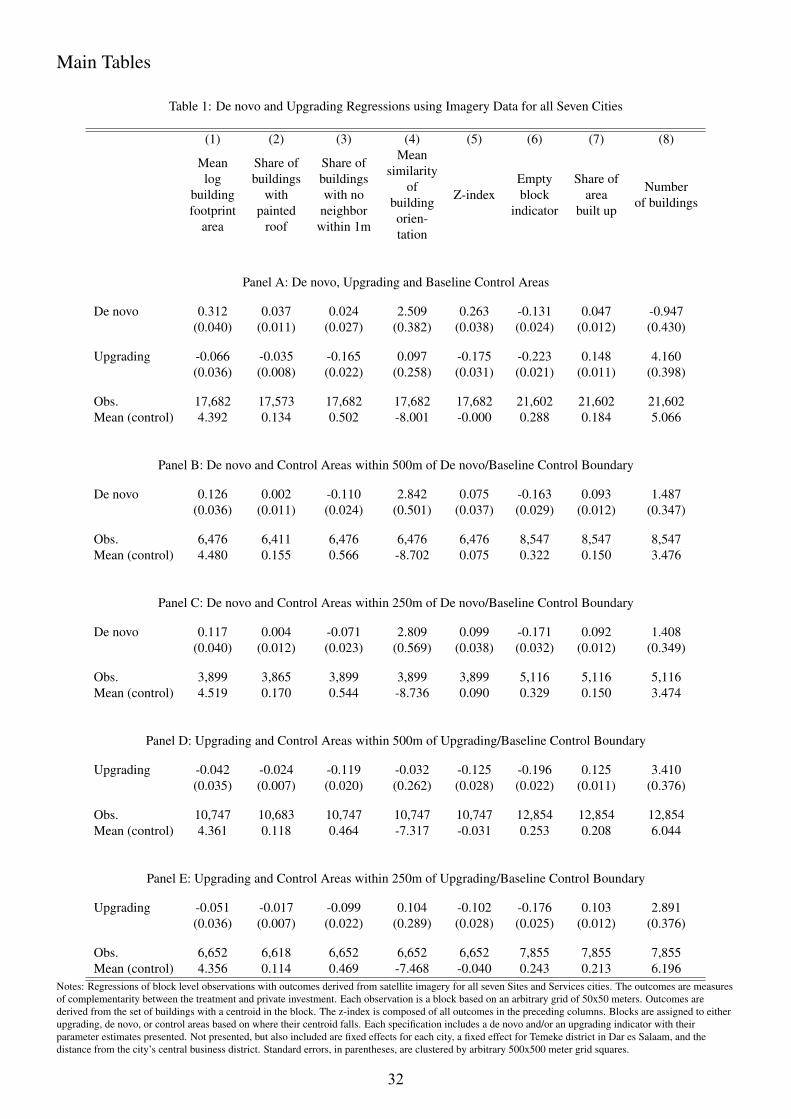
Main Tables

Table 1: De novo and Upgrading Regressions using Imagery Data for all Seven Cities

(1) (2) (3) (4) (5) (6) (7) (8)

Meanlog

buildingfootprint

area

Share ofbuildings

withpainted

roof

Share ofbuildingswith no

neighborwithin 1m

Meansimilarity

ofbuildingorien-tation

Z-indexEmptyblock

indicator

Share ofarea

built up

Numberof buildings

Panel A: De novo, Upgrading and Baseline Control Areas

De novo 0.312 0.037 0.024 2.509 0.263 -0.131 0.047 -0.947(0.040) (0.011) (0.027) (0.382) (0.038) (0.024) (0.012) (0.430)

Upgrading -0.066 -0.035 -0.165 0.097 -0.175 -0.223 0.148 4.160(0.036) (0.008) (0.022) (0.258) (0.031) (0.021) (0.011) (0.398)

Obs. 17,682 17,573 17,682 17,682 17,682 21,602 21,602 21,602Mean (control) 4.392 0.134 0.502 -8.001 -0.000 0.288 0.184 5.066

Panel B: De novo and Control Areas within 500m of De novo/Baseline Control Boundary

De novo 0.126 0.002 -0.110 2.842 0.075 -0.163 0.093 1.487(0.036) (0.011) (0.024) (0.501) (0.037) (0.029) (0.012) (0.347)

Obs. 6,476 6,411 6,476 6,476 6,476 8,547 8,547 8,547Mean (control) 4.480 0.155 0.566 -8.702 0.075 0.322 0.150 3.476

Panel C: De novo and Control Areas within 250m of De novo/Baseline Control Boundary

De novo 0.117 0.004 -0.071 2.809 0.099 -0.171 0.092 1.408(0.040) (0.012) (0.023) (0.569) (0.038) (0.032) (0.012) (0.349)

Obs. 3,899 3,865 3,899 3,899 3,899 5,116 5,116 5,116Mean (control) 4.519 0.170 0.544 -8.736 0.090 0.329 0.150 3.474

Panel D: Upgrading and Control Areas within 500m of Upgrading/Baseline Control Boundary

Upgrading -0.042 -0.024 -0.119 -0.032 -0.125 -0.196 0.125 3.410(0.035) (0.007) (0.020) (0.262) (0.028) (0.022) (0.011) (0.376)

Obs. 10,747 10,683 10,747 10,747 10,747 12,854 12,854 12,854Mean (control) 4.361 0.118 0.464 -7.317 -0.031 0.253 0.208 6.044

Panel E: Upgrading and Control Areas within 250m of Upgrading/Baseline Control Boundary

Upgrading -0.051 -0.017 -0.099 0.104 -0.102 -0.176 0.103 2.891(0.036) (0.007) (0.022) (0.289) (0.028) (0.025) (0.012) (0.376)

Obs. 6,652 6,618 6,652 6,652 6,652 7,855 7,855 7,855Mean (control) 4.356 0.114 0.469 -7.468 -0.040 0.243 0.213 6.196

Notes: Regressions of block level observations with outcomes derived from satellite imagery for all seven Sites and Services cities. The outcomes are measuresof complementarity between the treatment and private investment. Each observation is a block based on an arbitrary grid of 50x50 meters. Outcomes arederived from the set of buildings with a centroid in the block. The z-index is composed of all outcomes in the preceding columns. Blocks are assigned to eitherupgrading, de novo, or control areas based on where their centroid falls. Each specification includes a de novo and/or an upgrading indicator with theirparameter estimates presented. Not presented, but also included are fixed effects for each city, a fixed effect for Temeke district in Dar es Salaam, and thedistance from the city’s central business district. Standard errors, in parentheses, are clustered by arbitrary 500x500 meter grid squares.

32

Table 2: De novo and Upgrading Regressions using TSCP Survey Data for Mbeya, Mwanza, and Tanga

(1) (2) (3) (4) (5) (6) (7) (8) (9)Meanlog

buildingfootprint

area

Share ofbuildings

withmultiplestoreys

Share ofbuildings

witha good roof

Share ofbuildings

connected toelectricity

Share ofbuildings

with sewerageor septic

tank

Z-indexEmptyblock

indicator

Shareof

built uparea

Numberof

buildings

Panel A: De novo, Upgrading and Baseline Control Areas

De novo 0.456 0.114 -0.003 0.296 0.195 0.461 -0.138 0.110 0.715(0.055) (0.054) (0.008) (0.035) (0.049) (0.058) (0.041) (0.014) (0.304)

Upgrading -0.128 -0.088 -0.095 -0.076 -0.099 -0.344 -0.178 0.091 2.342(0.090) (0.027) (0.034) (0.049) (0.053) (0.104) (0.042) (0.018) (0.447)

Obs. 3,813 3,583 3,810 3,813 3,804 3,813 4,959 4,959 4,959Mean (control) 4.801 0.092 0.975 0.464 0.352 -0.000 0.289 0.127 2.549

Panel B: De novo and Control Areas within 500m of De novo/Baseline Control Boundary

De novo 0.469 0.096 -0.002 0.270 0.188 0.438 -0.130 0.113 0.864(0.057) (0.055) (0.006) (0.041) (0.049) (0.064) (0.037) (0.015) (0.280)

Obs. 2,031 1,995 2,031 2,031 2,028 2,031 2,715 2,715 2,715Mean (control) 4.782 0.099 0.981 0.468 0.389 0.030 0.300 0.104 2.012

Panel C: De novo and Control Areas within 250m of De novo/Baseline Control Boundary

De novo 0.451 0.072 -0.003 0.238 0.178 0.388 -0.139 0.104 0.847(0.060) (0.067) (0.008) (0.050) (0.059) (0.080) (0.044) (0.016) (0.276)

Obs. 1,223 1,203 1,223 1,223 1,220 1,223 1,644 1,644 1,644Mean (control) 4.766 0.145 0.983 0.479 0.382 0.064 0.322 0.100 1.926

Panel D: De novo and Entire City Control Areas

De novo 0.465 0.118 0.018 0.345 0.202 0.529 -0.359 0.152 1.637(0.046) (0.051) (0.008) (0.033) (0.044) (0.057) (0.039) (0.015) (0.223)

Obs. 23,173 22,126 23,146 23,173 23,037 23,173 42,409 42,409 42,409Mean (control) 4.876 0.110 0.946 0.488 0.399 0.022 0.461 0.096 1.707

Panel E: Upgrading and Control Areas within 500m to Upgrading/Baseline Control Boundary

Upgrading -0.166 -0.082 -0.100 -0.093 -0.121 -0.380 -0.156 0.078 2.123(0.094) (0.025) (0.035) (0.051) (0.055) (0.108) (0.044) (0.019) (0.470)

Obs. 2,062 1,851 2,059 2,062 2,056 2,062 2,583 2,583 2,583Mean (control) 4.864 0.098 0.970 0.522 0.347 0.042 0.246 0.163 3.275

Panel F: Upgrading and Control Areas within 250m to Upgrading/Baseline Control Boundary

Upgrading -0.157 -0.092 -0.126 -0.108 -0.164 -0.461 -0.162 0.075 1.874(0.105) (0.031) (0.044) (0.057) (0.057) (0.135) (0.053) (0.022) (0.528)

Obs. 1,189 1,069 1,188 1,189 1,185 1,189 1,515 1,515 1,515Mean (control) 4.808 0.127 0.967 0.499 0.379 0.043 0.270 0.152 3.309

Panel G: Upgrading Areas and Entire City Control Areas

Upgrading -0.220 -0.141 -0.080 -0.107 -0.122 -0.411 -0.301 0.123 3.252(0.078) (0.021) (0.035) (0.047) (0.039) (0.091) (0.041) (0.020) (0.420)

Obs. 23,090 21,977 23,063 23,090 22,956 23,090 42,251 42,251 42,251Mean (control) 4.876 0.110 0.946 0.488 0.399 0.022 0.461 0.096 1.707

Notes: Regressions of block level observations with outcomes derived from TSCP survey data for Mbeya, Mwanza, and Tanga. The outcomes are measures ofcomplementarity between the treatment and private investment. Each observation is a block based on an arbitrary grid of 50x50 meters. Outcomes are derivedfrom the set of buildings with a centroid in the block. The z-index is composed of all outcomes in the preceding columns. Blocks are assigned to eitherupgrading, de novo, or control areas based on where their centroid falls. Each specification includes a de novo and/or an upgrading indicator with theirparameter estimates presented. Not presented, but also included are fixed effects for each city and the distance from the city’s central business district. Standarderrors, in parentheses, are clustered by arbitrary 500x500 meter grid squares. Panels E and G display results for the sample of blocks covering the whole cityexcluding upgrading and de novo areas respectively.

33

Table 3: De novo and Upgrading Regressions using TSCP Survey Data for Mbeya, Mwanza, and Tanga with Owner Name FixedEffects

(1) (2) (3) (4) (5) (6)Log

buildingfootprint

area

Multistoreybuilding

Goodroof

Connectedto

electricity

Sewerage orseptic tank

Z-index

Panel A: Baseline Model without Name Fixed Effects

De novo 0.613 0.190 -0.022 0.355 0.219 0.502(0.078) (0.086) (0.018) (0.028) (0.050) (0.055)

Upgrading -0.009 -0.117 -0.044 0.029 -0.061 -0.136(0.094) (0.033) (0.020) (0.052) (0.039) (0.070)

Obs. 23,921 20,351 23,858 23,921 23,627 23,921Mean (control) 4.626 0.103 0.975 0.448 0.265 -0.000

Panel B: Owner Last Name Fixed Effects

De novo 0.798 0.191 -0.043 0.402 0.260 0.568(0.072) (0.107) (0.021) (0.032) (0.061) (0.065)

Upgrading 0.049 -0.158 -0.035 0.066 -0.028 -0.097(0.082) (0.050) (0.015) (0.050) (0.031) (0.065)

Obs. 11,122 8,698 11,082 11,122 10,899 11,122Mean (control) 4.626 0.103 0.975 0.448 0.265 -0.000

Panel C: Owner Full Name Fixed Effects

De novo 0.545 0.180 0.022 0.249 0.035 0.419(0.113) (0.101) (0.043) (0.089) (0.109) (0.135)

Upgrading -0.008 -0.053 -0.008 0.309 0.025 0.078(0.109) (0.052) (0.027) (0.079) (0.081) (0.082)

Obs. 6,493 4,655 6,457 6,493 6,311 6,493Mean (control) 4.626 0.103 0.975 0.448 0.265 -0.000

Notes: Regressions of unit level observations with outcomes derived from TSCP survey data for Mbeya, Mwanza, and Tanga. The outcomes are measures ofcomplementarity between the treatment and private investment. Each observation is a unit in a building. Outcomes are measured at the building level. Thez-index is composed of all outcomes in the preceding columns. Units are assigned to either upgrading, de novo, or control areas based on where their building’scentroid falls. Each specification includes a de novo and/or an upgrading indicator with their parameter estimates presented. Not presented, but also includedare fixed effects for each city and the distance from the city’s central business district. Standard errors, in parentheses, are clustered by arbitrary 500x500 metergrid squares. Panel A displays results for the full sample of units inside de novo, upgrading, and baseline control areas. Panel B displays results adding unitowner last name fixed effects and further restricting the sample by dropping singletons; keeping only last name owners that appear more than once in thesample. Panel C displays results adding owner full (first and last) name fixed effects and further restricting the sample by dropping singletons; keeping only fullname owners that appear more than once in the sample.

34

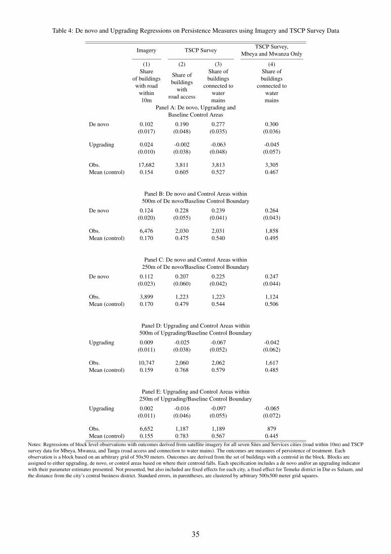
Table 4: De novo and Upgrading Regressions on Persistence Measures using Imagery and TSCP Survey Data

Imagery TSCP SurveyTSCP Survey,

Mbeya and Mwanza Only

(1) (2) (3) (4)Share

of buildingswith road

within10m

Share ofbuildings

withroad access

Share ofbuildings

connected towatermains

Share ofbuildings

connected towatermains

Panel A: De novo, Upgrading andBaseline Control Areas

De novo 0.102 0.190 0.277 0.300(0.017) (0.048) (0.035) (0.036)

Upgrading 0.024 -0.002 -0.063 -0.045(0.010) (0.038) (0.048) (0.057)

Obs. 17,682 3,811 3,813 3,305Mean (control) 0.154 0.605 0.527 0.467

Panel B: De novo and Control Areas within500m of De novo/Baseline Control Boundary

De novo 0.124 0.228 0.239 0.264(0.020) (0.055) (0.041) (0.043)

Obs. 6,476 2,030 2,031 1,858Mean (control) 0.170 0.475 0.540 0.495

Panel C: De novo and Control Areas within250m of De novo/Baseline Control Boundary

De novo 0.112 0.207 0.225 0.247(0.023) (0.060) (0.042) (0.044)

Obs. 3,899 1,223 1,223 1,124Mean (control) 0.170 0.479 0.544 0.506

Panel D: Upgrading and Control Areas within500m of Upgrading/Baseline Control Boundary

Upgrading 0.009 -0.025 -0.067 -0.042(0.011) (0.038) (0.052) (0.062)

Obs. 10,747 2,060 2,062 1,617Mean (control) 0.159 0.768 0.579 0.485

Panel E: Upgrading and Control Areas within250m of Upgrading/Baseline Control Boundary

Upgrading 0.002 -0.016 -0.097 -0.065(0.011) (0.046) (0.055) (0.072)

Obs. 6,652 1,187 1,189 879Mean (control) 0.155 0.783 0.567 0.445

Notes: Regressions of block level observations with outcomes derived from satellite imagery for all seven Sites and Services cities (road within 10m) and TSCPsurvey data for Mbeya, Mwanza, and Tanga (road access and connection to water mains). The outcomes are measures of persistence of treatment. Eachobservation is a block based on an arbitrary grid of 50x50 meters. Outcomes are derived from the set of buildings with a centroid in the block. Blocks areassigned to either upgrading, de novo, or control areas based on where their centroid falls. Each specification includes a de novo and/or an upgrading indicatorwith their parameter estimates presented. Not presented, but also included are fixed effects for each city, a fixed effect for Temeke district in Dar es Salaam, andthe distance from the city’s central business district. Standard errors, in parentheses, are clustered by arbitrary 500x500 meter grid squares.

35

Table 5: De novo and Upgrading Regressions for Rounds 1 and 2 using Imagery Data for all Seven Cities

Meanlog

buildingfootprint

area

Share ofbuildingswith no

neighborwithin 1m

Meansimilarity

ofbuildingorien-tation

Shareof buildingswith road

within10m

Z-index(including

roads)

Emptyblock

indicator

Share ofarea

built up

Numberof buildings

De novo 1 0.372 0.042 3.082 0.137 0.378 -0.066 0.040 -1.532(0.051) (0.034) (0.450) (0.022) (0.043) (0.029) (0.016) (0.599)

De novo 2 0.041 -0.110 1.556 0.015 -0.015 -0.209 0.079 1.677(0.043) (0.034) (0.814) (0.015) (0.031) (0.046) (0.018) (0.394)

Upgrading 1 -0.208 -0.270 0.734 0.029 -0.211 -0.128 0.171 6.028(0.059) (0.034) (0.304) (0.018) (0.042) (0.024) (0.018) (0.747)

Upgrading 2 0.025 -0.096 -0.400 0.017 -0.071 -0.282 0.133 2.993(0.039) (0.024) (0.389) (0.011) (0.028) (0.028) (0.013) (0.368)

Obs. 17,682 17,682 17,682 17,682 17,682 21,602 21,602 21,602Mean (control) 4.392 0.502 -8.001 0.154 -0.000 0.288 0.184 5.066

Notes: Regressions of block level observations with outcomes derived from satellite imagery for all seven Sites and Services cities. The outcomes are measuresof complementarity between the treatment and private investment. Each observation is a block based on an arbitrary grid of 50x50 meters. Outcomes arederived from the set of buildings with a centroid in the block. The z-index is composed of all outcomes in the preceding columns. Blocks are assigned to eitherupgrading, de novo, or control areas based on where their centroid falls. Each specification includes de novo round 1, de novo round 2, upgrading round 1, andupgrading round 2 indicators with their parameter estimates presented. Not presented, but also included are fixed effects for each city, a fixed effect for Temekedistrict in Dar es Salaam, and the distance from the city’s central business district. Standard errors, in parentheses, are clustered by arbitrary 500x500 meter gridsquares.

36

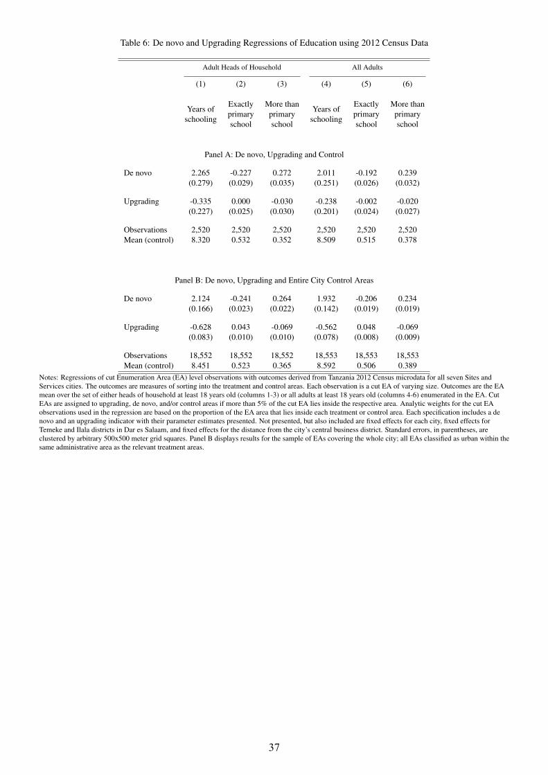
Table 6: De novo and Upgrading Regressions of Education using 2012 Census Data

Adult Heads of Household All Adults

(1) (2) (3) (4) (5) (6)

Years ofschooling

Exactlyprimaryschool

More thanprimaryschool

Years ofschooling

Exactlyprimaryschool

More thanprimaryschool

Panel A: De novo, Upgrading and Control

De novo 2.265 -0.227 0.272 2.011 -0.192 0.239(0.279) (0.029) (0.035) (0.251) (0.026) (0.032)

Upgrading -0.335 0.000 -0.030 -0.238 -0.002 -0.020(0.227) (0.025) (0.030) (0.201) (0.024) (0.027)

Observations 2,520 2,520 2,520 2,520 2,520 2,520Mean (control) 8.320 0.532 0.352 8.509 0.515 0.378

Panel B: De novo, Upgrading and Entire City Control Areas

De novo 2.124 -0.241 0.264 1.932 -0.206 0.234(0.166) (0.023) (0.022) (0.142) (0.019) (0.019)

Upgrading -0.628 0.043 -0.069 -0.562 0.048 -0.069(0.083) (0.010) (0.010) (0.078) (0.008) (0.009)

Observations 18,552 18,552 18,552 18,553 18,553 18,553Mean (control) 8.451 0.523 0.365 8.592 0.506 0.389

Notes: Regressions of cut Enumeration Area (EA) level observations with outcomes derived from Tanzania 2012 Census microdata for all seven Sites andServices cities. The outcomes are measures of sorting into the treatment and control areas. Each observation is a cut EA of varying size. Outcomes are the EAmean over the set of either heads of household at least 18 years old (columns 1-3) or all adults at least 18 years old (columns 4-6) enumerated in the EA. CutEAs are assigned to upgrading, de novo, and/or control areas if more than 5% of the cut EA lies inside the respective area. Analytic weights for the cut EAobservations used in the regression are based on the proportion of the EA area that lies inside each treatment or control area. Each specification includes a denovo and an upgrading indicator with their parameter estimates presented. Not presented, but also included are fixed effects for each city, fixed effects forTemeke and Ilala districts in Dar es Salaam, and fixed effects for the distance from the city’s central business district. Standard errors, in parentheses, areclustered by arbitrary 500x500 meter grid squares. Panel B displays results for the sample of EAs covering the whole city; all EAs classified as urban within thesame administrative area as the relevant treatment areas.

37

For Online Publication - Data Appendix for:

Planning Ahead for Better Neighborhoods: Long RunEvidence from Tanzania

Guy Michaels (LSE) Dzhamilya Nigmatulina (LSE) Ferdinand Rauch (Oxford)

Tanner Regan (LSE) Neeraj Baruah (LSE) Amanda Dahlstrand-Rudin (LSE)

This data appendix is organized as follows. We begin with a short description of the background

for the Sites and Services projects and a discussion of how the de novo plots were allocated. We then

explain how we measure the treatment and control areas in the different cities. We then describe

the three main datasets: the first comes from imagery data; the second from the Tanzania Strategic

Cities Project Survey (TSCP); and the third comes from Tanzanian census micro data. Finally, we

discuss other auxiliary datasets, including additional census data (at a coarser level of aggregation);

land values data; data on project costs; population data for 2002; Finally, we explain how we make

currency conversions.

Project Background and treatment

Background

The Sites and Services projects took place in seven Tanzanian cities. Twelve de novo areas (greenfield

investments) and twelve slum upgrading areas (upgraded squatter settlements). The project was

rolled out in two rounds - the first in 1974-1977 and the second 1977-1984. In the First Round, the

World Bank treated the northwest of Dar es Salaam (Kinondoni) and Mbeya with both de novo

and upgrading and Mwanza with de novo investment only. In the Second Round the two types

of treatment took place in the southeast of Dar es Salaam (Temeke), Tanga, Tabora, Morogoro and

Iringa. The number of de novo and upgrading plot surveyed in each round is reported in Appendix

Table A4. Both stages included investments in roads and roadside drainage (open earth ditches)

along them and a mix of public buildings (typically schools, dispensaries and health centers). In

some cases street lights near the public buildings were also provided. Round 1 areas and Round 2

upgrading areas (but not Round 2 de novo areas) also benefitted from water mains.

Allocation of de novo plots

Plots were allocated to beneficiaries according whose i) houses were demolished in the upgrading

areas ii) income was in the range of 400-1000 Tanzanian shilling (Tsh) a month. The income range

was meant to target the 20th-60th percentiles of countrywide incomes (Kironde, 1991). According

to project completion reports (World Bank, 1984 and World Bank, 1987), between 50% and 70% of

all project beneficiaries belonged to the target population. There was some evidence (World Bank,

38

1987) that a number of more affluent individuals obtained some of the plots after they had not been

developed by initial beneficiaries.

Selection of Treatment and Control Areas

We use a variety of historical maps, satellite and aerial photos to define the exact boundaries of

treatment. For Dar, Iringa, Tabora, Tanga, and Morogoro, the World Bank Project Appraisals (World

Bank, 1974a and World Bank, 1977b) provided maps of the planned boundaries of the upgrading and

de novo sites. In Dar, two maps were available, from 1974 and 1977, differing slightly for Mikocheni

area. For all areas except Tandika and Mtoni, we chose to use the 1974 map, as it appeared more

precise in following the terrain and the roads. However, for Tandika and Mtoni we had to use the

1977 map, because these areas were part of the Second Round which was not included in the earlier

1974 map.

For the two remaining cities, Mbeya and Mwanza, the maps from the project appraisal were not

available. Therefore, for Mbeya we asked three experts to draw the boundaries of treatment. These

experts were Anna Mtani and Shaoban Sheuya from Ardhi University, who both worked on the first

round of Sites and Services project, and Amulike Mahenge from the Ministry of Land, who was the

Municipal Director in Mbeya.

To delineate the treatment areas in Mwanza we obtained cadastral maps dating back to 1973 from

the city municipality. Since in Mwanza the treatment included only de novo plots, the cadastral map

was sufficient to get the information for the intended treatment areas. We define the treatment area

as covering the numbered plots that were of a size that (approximately) fitted the project descriptions

(288 square meters); we also include public buildings into the treatment areas, to be consistent with

the procedure in other cities. This procedure gives us a comprehensive picture of the twelve de novo

and twelve upgrading neighborhoods across all seven cities.

To define our control areas, along with the historical World Bank maps from the Appraisal reports

(World Bank, 1974a and World Bank, 1977b), we use historical topographic maps, and satellite and

aerial images taken just before the dates of the treatment. We assign all undeveloped ("greenfield")

land within 500 meters of any treatment border to our set of control areas. However, as we explain

in more detail below, we exclude areas that were either designated for non-residential use, or that

were developed prior to treatment, or that are uninhabitable. Our rationale for looking at greenfield

areas as controls because we want a clear counterfactual for the de novo areas. We have no “nat-

ural” counterfactual for the upgraded squatter areas, because we do not observe untreated squatter

areas in the vicinity. The 500 meter cut-off reduces the risk of substantial heterogeneity in locational

fundamentals. As part of our analysis we also focus on areas that are even closer to the boundaries

between areas.

In order to know what had been previously developed, we used any historical maps or imagery

as close to the treatment date as we could find. We used all planned treatment maps. These include

the 1974 and 1977 maps for Dar es Salaam and the 1977 maps for Morogoro, Iringa, Tanga and Tabora

39

(World Bank 1987); the 1973 cadastral map of Mwanza (Mwanza City Municipality, 1973); satellite

images from 1966 (United States Geological Survey 2015); aerial imagery from 1978 for Tabora and

topographic maps from 1967 1974, and 1978 for Tabora, Iringa and Morogoro (Directorate of Overseas

Surveys 2015). All areas (with some minor exceptions described below) were covered by at least one

source. Satellite images and maps also confirm that the areas designated as de novo were indeed

unbuilt before the Sites and Services program was implemented.

We use all these data to determine which areas within 500 meter of Sites and Services areas to

exclude from our baseline control group. Our rules for exclusion from the control areas are as fol-

lows. First, we exclude areas that were planned for non-residential use. These were indicated on

the planned treatment map for industrial or governmental use. Second, we exclude areas that were

developed before the Sites and Services projects began. These were either indicated as houses or

industrial areas on topographic maps, or visibly built in the historical satellite images. Third, we ex-

clude uninhabitable areas, for example, those off the coast. Finally, in the case of Mwanza (where we

had to infer the treatment areas) we applied additional criteria for exclusion. In this case we exclude

large numbered plots and all unnumbered plots, which do not seem to fit the description of de novo

plots. We also exclude areas where the treatment areas are truncated at the edge, since we do not

know where the exact boundary of treatment is. In this case we drew rectangles perpendicular to the

map edge where the treatment area is truncated, and exclude the area within them.59 Further details

on defining exclusion areas are outlined in Table A14.

Thus, our treatment maps show upgrading, de novo and control areas, as well as excluded areas.

Moreover, with these appropriately defined control areas net of excluded locations, we can analyze

present day outcomes using boundaries between control areas and de novo areas, and between con-

trol areas and upgrading areas.

Dataset 1: Imagery data

Buildings

To study the quality of housing we use Worldview satellite images (DigitalGlobe 2016), which pro-

vide grayscale data at resolution of approximately 0.5 meters along with multispectral data at a

resolution of approximately 2.5 meters. 60 We employed a company (Ramani Geosystems) to trace

out the building footprints from these data for six of the seven cities. For the final city, Dar es Salaam,

we used building outlines from a different, freely available, source - Dar Ramani Huria (2016).

We derive the following indicators of building quality using the building outlines: the logarithm

of building footprint, the distance between each building and its neighbor, building orientation rel-

59We include in the baseline control areas (minor) areas where there is no pre-treatment data, because they are verysparse and are located near other empty areas.

60The images were taken at different dates: Iringa (2013), Mbeya (2014), Morogoro (2012), Mwanza (2014), Tabora (2011),Tanga (2012) and there are two separate images for two districts in Dar es Salaam: Kinondoni (2015) and Temeke(2014)

40

ative to its neighbors and, finally the distance to the nearest road using ArcGIS tools. Details on the

derivation of these variables are described in Appendix Table A15.

We use two different approaches to analyze the data: building level outcomes and outcomes at

the level of 50 x 50 meter blocks. For building level outcomes each variable is simply the measure for

that given building. For grid cell outcomes we average each measure and indicator to get averages

and shares. To do that, we begin with an arbitrary grid of 50 x 50 meter blocks. If a block is divided

between de novo, upgrading, and control areas, we attribute the cell to the area where its centroid

lies. Finally, we match into each cell the buildings whose centroids fall within it. This allows us to

additionally measure three variables: the share of built up area in the cell, the count of buildings in a

cell and whether the cell is empty. These variable descriptions are summarized in Table A15.

Roofs

To study the quality of roofs, we use the same Worldview satellite images as we did for the build-

ing outcomes above. The objective is to separate painted roofs (which are less prone to rust) from

unpainted tin roofs (rusted or not), in order to get a measure for roof quality that captures more

variation than the TSCP survey indicator for good roofs. The cut-off between painted and unpainted

roofs was chosen also because we had evidence from our initial field investigation that the painted

roofs are considerably more expensive.

To this end, we create an algorithm through which ArcGIS and Python can separate painted from

unpainted roofs for each satellite image of the seven Sites and Services cities. Before running the

algorithm, we created unique color bins which would identify each type of roof material. These bins

are three-dimensional sections of the red-green-blue space that correspond to different colors, which

we think of as either painted roofs (e.g. painted red, green, blue 61) or unpainted ones (e.g. tin,

rusted, and bright tin 62). We defined the bins through a process of sampling pixels from each roof

material type, identifying the color bins to which the pixels belong, and iteratively narrowing the

bins for each roof type until they were mutually exclusive. Since each satellite image was slightly

different in terms of sharpness, brightness and saturation, we sampled pixels from each image and

created city-specific bands.

The algorithm is then applied to each city with its unique color bins. The algorithm works by

reading the values of the color spectrum for red, green and blue of each pixel of a roof, and comparing

these values to the above-mentioned unique bands of the color spectrum identifying painted, rusted

and tin roofs. We assign to each roof the color bin that contains the plurality of pixels, and this

indicates whether we classify it as a painted roof or not.

61Apart from red, green and blue we also had a bin for brown painted roofs in Kinondoni, since only in that imagewe noticed a large number of painted roofs that had a brown color, either due to image particularities or geographicallyvarying preferences for brown painted roofs.

62In Iringa and Mwanza we did not have the category bright tin since the particularities of the image or the conditionsof the day when the image was taken resulted in other roofs than tin also being very bright in these cities.

41

Roads

For all seven cities we used road data from Openstreetmap (2017). We had to clean these data in

some locations using ArcGIS and Python, so that we only use roads that seem wide enough for a

single car to pass through (we eliminated "roads" between buildings that were less than one meter

apart). Following this automated procedure, we cleaned the road data manually to identify roads

that appear passable to a single car.

Dataset 2: Tanzanian Strategic Cities Project Survey

For three cities, Mbeya (in southwest Tanzania), Tanga (in northeast Tanzania), and Mwanza (in

northwest Tanzania) we have detailed building-level data from the Tanzanian Strategic Cities Project

(TSCP) which is a World Bank project implemented by the Prime Minister’s Office of Regional Ad-

ministration and Local Government (World Bank 2010). These surveys were carried out by the Tan-

zanian government from 2010-2013. We use these data to build a more detailed picture of building

quality in the areas we study.

The data arrived in raw format, with multiple duplicated records of each building and unit and

many of these duplicate observations with missing data. We used the following ruled to identify the

unique observations. Buildings are identified by ‘Building Reference Numbers’ (BRN) and building

units by BRN-units.

Rules for Excluding Buildings

1. Drop exact duplicates. i.e. if multiple buildings have all the same variables (including IDs)

only keep one of them (dropped 1,202,669 observations).

2. Of all remaining observations with a duplicate BRN, drop all where all ‘variables of interest’

are missing. Variables of interest are an extensive list and comprise much more than what is

used in the analysis of this paper (dropped 166,131 observations).

3. Of all remaining observations with a duplicate BRN, keep the observations with strictly more

non-missing variables of interest (dropped 12,842 observations).

4. Of all remaining observations with a duplicate BRN, rank by ‘information provider’ and keep

the observations with a strictly higher rank (dropped 15,486 observations).

5. Of all remaining observations with a duplicate BRN, for a set of observations with the same

BRN, replace with missing all variables where the records are inconsistent. For example, if

there are two observations with the same BRN and both have ‘2’ for number of stories there is

no inconsistency. But if one has ‘1’ number of rooms while the other has ‘2’: replace the number

of rooms with missing for both.

42

6. Of all remaining observations with a duplicate BRN all duplicate BRNs will have exactly the

same records, keep only one record for each BRN (dropped 27,483 observations).

7. There are no longer any duplicate BRNs. We drop 35,912 unique buildings from the records

that do not match a building in one of the city shapefiles of building footprints.

8. We drop 38,180 buildings from the records that are coded as outbuildings.

9. We drop 596 buildings that do not match to a unit.

10. Finally, we are left with 119,914 buildings all with at least one corresponding unit.

Rules for Excluding Building Units

1. Drop exact duplicates, for example, if multiple units have all the same variables (including IDs)

only keep one of them (dropped 1,288,430 observations).

2. Of all remaining observations with a duplicate BRN-unit, drop all where all variables of interest

are missing. Variables of interest are an extensive list and comprise much more than what is

used in the analysis of this paper (dropped 221,134 observations).

3. Of all remaining observations with a duplicate BRN-unit, keep the observations with strictly

more non-missing variables of interest (dropped 6,383 observations)

4. Of all remaining observations with a duplicate BRN-unit, for a set of observations with the

same BRN-unit, replace with missing all variables with mismatched records within the set. i.e.

if there are two observations with the same BRN-unit and both have ‘2’ for number of toilets:

do nothing, if one has ‘1’ number of rooms while the other has ‘2’: replace the number of rooms

with missing for both.

5. There are no longer any duplicate BRN-units. We drop 32,322 units from the records that do

not match a building in one of the city shapefiles of building footprints.

6. We drop 3,216 units from the records that are coded as outbuildings.

7. We do not need to drop any more units, since all remaining units match to a building.

8. Finally, we are left with 154,734 units all with a corresponding building.

From the building data set we exclude all buildings categorized as “Outbuildings” (sheds, garages,

and animal pens) from the analysis. This leaves us with a sample of buildings that are used mostly

for residential purposes, although a small fraction also serve commercial or public uses.

For these buildings in analysis we use the logarithm of building footprint; connection to elec-

tricity; connection to water mains; having at least basic sanitation (usually a septic tank and in rare

cases sewerage); having good (durable) roof materials; having more than one story; and having road

access. These variables and the explanation of how they are constructed are outlined in Table A16.

43

Rebuilding Rate

In addition to using TSCP data for the main analysis, we also use the TSCP data to calculate the rate

at which buildings are rebuilt, which we use in the model section. We use a dataset that includes the

construction year and latest rebuilding year for a sample of houses up to the year 2013.

In all three cities the default value for the "Year Built" and "Year Rebuilt" variables was apparently

2000, hence we had no way to distinguish whether the building was truly rebuilt in 2000, or the data

was missing. We therefore drop all observations with year 2000 for both of these variables from the

analysis and are left with 10% of total observations of buildings. Further, we only observe the latest

reconstruction year, rather than all reconstruction years.

Dataset 3: 2012 Tanzanian Census Micro Data Extract

This extract was obtained through a contact from Tanzanian Census Bureau. As opposed to the Tan-

zanian census data that can be obtained online at the IPUMS repository, this data was on individual

level. We matched these census observations from this extract to geographical areas using EA iden-

tifiers in the census extract. Using shapefiles of EAs (with the same identifiers) from the Tanzanian

Census 2012, also obtained from the same contact, we could match the census data observations to

our treatment and control areas. The process of matching EAs to treatment areas (de novo, control

and upgrading) was done through Python and ArcGIS.

In case an EA straddled two (or more) of the treatment and control areas, we performed a cut of

that EA in ArcGIS so that two (or more) parts were created, each part belonging to each treatment

and control area. We could then use this information to weight remove the census data observations

which belonged to an EA whose area inside a treatment and control area was less than 5% of the

entire EA area. We also used the information on how large a part of the EA was inside a treatment

or control area to create analytic weights based on included EA proportion for Table 6, as well as for

the adjusted population numbers used for analytic weights in Table A12.

We then took means of the variables of interest (mainly three variables which were all different

codings of the variable for educational attainment) over the cut EAs. We counted the number of

observations that contributed to the mean, to be used in the robustness check of Table 6 with analytic

weights. We also created variables for the longitude and latitude coordinates of the centroids of the

cut EAs in both degrees and meters, using ArcGIS and Python.

To create the dataset where we use entire cities as controls, we used Python and ArcGIS to select

the EAs that belonged to the same administrative district and region as the treatment areas. Then

we created means of the education variables also in these EAs, as well as counted the number of

observations that contributed to the mean, to be used in the robustness check of Table 6 with analytic

weights (Table A17).

44

IPUMS 2012 Tanzanian Census by Region

We used this data, downloaded from the IPUMS online repository of country censuses, in order

to check the above-mentioned microdata extract from the same census for correctness. This was

done in particular for the education variable which had been cleaned by IPUMS staff to include

many observations recorded as having “never attended” school. The microdata that we had received

directly from the Tanzanian Census Bureau had many missing values for the education variable, and

none coded as never having attended school. The missing values in the micro-data followed the

same pattern as the “never attended” in the IPUMS data, which contributed to our decision to code

them as “Zero years of schooling”. We also checked age and gender patterns in the microdata which

also confirmed this.

Land Values

Matching Land Value Data to Enumeration Areas

We have an Excel sheet titled “RATES LAND VALUE MIKOA 10 2012.xls”, which we received from

the Kinondoni Municipal council, but were told that it was created by the Ministry of Lands, with

min, mean, and max land values for different neighborhoods in Tanzania. We can identify these

neighborhoods by four string identifiers: region, district, location, and streets. To locate neighbor-

hoods we match them based on the 2002 enumeration area (EA) shapefile, which contains string iden-

tifiers for region, district, location, and vill_stree (we consider ‘vill_stree’ comparable with ‘streets’

from the land values table).

Land Use

The Excel table has different min, mean, and max land values by land use. There are typically four

categories: Residential, commercial, commercial/residential, and institutional. Though the differen-

tiation of land values across uses is mechanical (commercial is 1.4* res, com/res is 1.1*res, institu-

tional is the same as res). Sometimes there is also a category for ‘beach plots’. Throughout we use

mean land values from the residential categories only.

Spatially Mapping Land Values

We merge EA boundaries to land value observations using the four identifiers: region, district, lo-

cation, and streets. Each entry in the land value table I treat as an observation, often this contains a

group of ‘streets’. Typically there are many EAs per land value observation, so each observation in

the land values table is matched to a large group of EA boundaries. Then we dissolve the EA bound-

aries to have a single spatial unit for each entry in the land value sheet. I plot the mean residential

land rate for each spatial unit.

45

Results

The merged areas are quite large. Some roughly match our treatment areas:

1. Sinza – one unit at 240,000TSh

2. Manzese A – three partial units all at 65,000TSh

3. Manzese B – split in half, one at 65,000TSh the other at 50,000TSh

4. Kijitonyama – one unit at 325,000TSh

The other two do not match as well:

1. Mikocheni – contained by a much larger unit at 125,000TSh

2. Tandika/Mtoni – overlaps many areas of values; 40,000TSh, 30,000TSh, 50,000TSh, and 18,000TSh

These values per square meter put us in the ballpark of 125,000-325,000 TSh (2017 US$80-220) in

de novo and 18,000-65,000 TSh (2017 US$10-40) in upgrading. For the areas where we have better

matched data the ranges are 240,000-325,000 TSh (2016 US$160-220) in de novo and 50,000-65,000

TSh (2017 US$30-40) in upgrading.

Project Costs

The total cost of Round 1 was $15 million in 1977 USD ($60m in 2017 USD) where 53% was spent on

direct costs (World Bank 1984). Direct costs payed for infrastructure (largest cost component, 62%),

consultants (16%), land compensation (11%) and a few other costs. This investment covered a total of

23,161 plots: 8,527 de novo plots and 14,634 upgrading plots. This excludes the loans scheme, which

later failed because of poor repayment rates, and loan allocation.63

Round 2 cost $27 million in 1982 USD ($70m in 2017 USD) where 70% was spent on direct costs,

paying for a total of 22,106 plots: 1,978 de novo plots and 20,128 upgrading plots (World Bank 1987).

The First Round project reports (World Bank 1974a and 1984) indicate that the total infrastructure

investment costs per area in de novo and upgrading were very similar. The project report for Round

1 provided costs separately for de novo and upgrading areas (World Bank, 1984). However only

infrastructure investment differed for the two types of treatment, while land compensation, equip-

ment, and consultancy costs were reported as split 50-50 between de novo and upgrading. Direct

costs by treatment were $19 million in de novo and $15 million in upgrading areas (in 2017 USD).

To get costs per unit area we normalize by total area covered by each treatment type in Round 1 (8.5

63House improvement & construction loans (Tsh 4,000-10,000 in 1977 or 2017 US$2,000-5,000) were also arranged for tohelp beneficiaries build and improve their existing houses. However, only about 4,500 loans were allocated, most to thebeneficiaries of the first stage of the project. Beneficiaries had to meet strict national building codes and a minimum valueor cost of Tsh 15,000 or 2017 US$8,000, in high density areas) and THB did not have funds to meet demand in a timelymanner.

46

square kilometers in de novo and 6.5 square kilometers in upgrading). This gave costs for de novo

and upgrading areas of $2.20 and $2.37 per square meter respectively (in 2017 USD).

Further, in order to compare with present day land values (per plot area) we would like an esti-

mate of costs per unit of treated plot area. Due to data limitations we can only do that for de novo

neighborhoods where the reports give both plot counts and plot areas. Our calculations suggest an

upper bound cost of $8 per square meter of treated plot area (in 2017 USD).64

An alternative way to look at costs is to break them down by plot which we can do for both

de novo and upgrading areas. According to the report there were 8,527 de novo plots and 14,634

upgrading plots in Round 1. We can divide the direct costs of de novo and upgrading areas by

their plot counts to get $2,200 and $1,000 per plot respectively (in 2017 USD). The difference in costs

reflects both the larger size of the de novo plots and the larger share of allocated to public amenities

(such as roads).

Most of the costs were, unsurprisingly, due to infrastructure investment, which accounted for

around 60-70 percent of the First Round costs and around 55 percent of the Second Round costs. Land

compensation accounted for 10-12 percent in the First Round and 25 percent in the Second Round.

The remainder - around 20-25 percent - covered equipment and consultancy.65 Second Round costs

per plot were similar to those of the First Round, but the reports do not separate the respective shares

of de novo and upgrading (World Bank 1977b and 1987).

Cost Recovery

Costs were meant to be recovered through land rent (4% of land value a year) and service charge (the

cost of infrastructure provider), but assessment of parcels was long and interim charge well below

the adequate amount to cover the costs (100 Tsh/year or 2017 US$51) was imposed. Collection rates

were low and not timely.

Population data for 2002

To calculate the population density in each of the neighborhoods, we use data on population by

enumeration areas from the 2002 Tanzanian Census (Tanzania National Bureau of Statistics 2011).

In cases where an entire enumeration area falls into a Sites and Services neighborhood, we assign

its entire population to that neighborhood. When only a fraction of an enumeration area falls into

a Sites and Services neighborhood, we assign to the neighborhood the fraction of the enumeration

area population that corresponds to the fraction of the land area that lies within the neighborhood.

The mean number of enumeration areas matched to each neighborhood is 33 for de novo areas and

64To calculate the costs per square meter of each plot, we use the planned areas of de novo plots from Appraisal report 1(World Bank, 1974a); the planned area was 288 square meters, except for 8.56% of the plots (those in Mikocheni) where itwas 370 square meters. Taking the weighted average at 295 square meters, we can divide the de novo direct costs by totalplot area treated to get $7.5 per square meter.

65In addition, approximately 4,500 loans were allocated, over 90 percent of which were given to First Round plot owners.It seems that cost recoupment progressed slowly, and we do not know exactly how much was eventually paid back.

47

35 for upgrading areas. We also have complete population counts from the 2012 Tanzanian census,

but these data are reported in coarser, areas, and using these to measure population likely results in

more measurement error. Population counts are outlined in Table A4.

Conversion to 2017 US Dollars

All monetary values in the paper are reported in their source units and also converted to 2017 US

dollars (2017 US$). To calculate the dollar values we used the exchange rates to contemporaneous

year US$ from Penn World Tables 9.0 (Feenstra et al., 2015). Then we used the US CPI factors to bring

the value to 2017 US$.

References for the Data Appendix

DigitalGlobe. 2016. "Worldview Satellite Imagery." (Worldview satellite images on the slums

in the Tanzanian cities Iringa (2013), Mbeya (2014), Morogoro (2012), Mwanza (2014), Tabora (2011),

Tanga (2012) and two districts of Dar es Salaam: Kinondoni (2015) and Temeke (2014))

Dar Ramani Huria. 2016. "Community-Based Mapping Project in Dar es Salaam."

http://ramanihuria.org/data/ (accessed May 25, 2017).

Directorate of Overseas Surveys. 2015. "Aerial Imagery and Topographic maps from 1:2,500 to

1:50,000."

Feenstra, Robert C., Robert Inklaar and Marcel P. Timmer. 2015, "The Next Generation of the

Penn World Table" American Economic Review, 105(10), 3150-3182. www.ggdc.net/pwt (accessed

September 12, 2017)

IPUMS International. 2017. “Tanzania Population Census 2012”

https://international.ipums.org/international/ (accessed June 20, 2017)

Kinondoni Municipality. Dar es Salaam, Tanzania. 2013. "Tax registry and plot shapefile, Dar es

Salaam: Kinondoni Municipality GIS department."

Lusugga Kironde, JM. 2017. Interview with authors, Dar es Salaam, August 2, 2017.

Mwanza City Municipality. 1973. “Mwanza Cadastral Maps”

Openstreetmap. 2017. “Road Shapefiles of Dar es Salaam, Iringa, Mbeya, Morogoro, Mwanza,

Tabora and Tanga” https://www.openstreetmap.org (accessed June 20, 2017)

Tanzania Ministry of Lands. 2012. "Rates Land Value Mikoa (Regions) 10 2012."

Tanzania National Bureau of Statistics. 2011. "Tanzania Population and Housing Census 2002."

Tanzania National Bureau of Statistics. 2014. "Tanzania Population and Housing Census 2012."

Tanzania National Bureau of Statistics. 2017. “2012 Census Shapefiles (machine readable data

files)”

United States Geological Survey. 2015. "Declassified Satellite Imagery from 1960-1972." United

States Geological Survey, Reston, VA.

World Bank. 1974a. "Appraisal of National Sites and Services Project." Report No. 337a-TA,

Washington, DC: Urban Projects Department.

48

World Bank. 1977b. "Tanzania: The Second National Sites and Project." Report No. 1518a-TA,

Washington, DC: Urban Projects Department.

World Bank. 1984. "Completion Report: Tanzania - First National Sites and Services Project."

Re-port No. 4941, Washington, DC: Eastern Africa Regional Office.

World Bank. 1987. "Tanzania: The Second National Sites and Project." Report No. 6828, Washing-

ton, DC: Operations Evaluation Department.

World Bank. 2010. "Project Appraisal Document for a Tanzania Strategic Cities Project." Report

No. 51881-TZ, Washington, DC: Urban and Water Department.

World Bank. 2013. “Tanzania Strategic Cities Project Housing Survey”. Produced and shared by

President’s Office - Regional Administration and Local Government.

49

Appendix Tables and Figures

Figure A1. Payoffs as Functions of I2

Notes: This figure depicts three payoffs as functions of the levels of new public infrastructure, I2. The vertical axis is payoffs, the horizontal axis is the level ofinvestment I2. The thick blue line is the payoff, Pi1, from the initial level of infrastructure, I1, therefore it does not vary with I2. The red line, Pi1I2, is thepayoff from not rebuilding one’s house as I2 grows. The dashed green line is the payoff, Pi2, from upgrading your house as I2 grows. Although initially thepayoff of not rebuilding is higher, it soon reaches a critical point (I2crit), where the red and dashed green lines intersect and an agent is indifferent betweenupgrading and not.

50

Table A1: Model Table

Scenario1a:

(Baseline)

Scenario1b:

Baselinewith lessweight on

infra-structure

Scenario1c:

Baselinewith lesspatience

Scenario1d:

Baselinewith

Boston-level

rebuilding

Scenario1e:

Baselinewith much

higherbuilding

costs

Scenario 2:credit

constraintsincumbents

inupgrading

cannotbuild any

better thanq1

Scenario 3:land expro-

priationrisk of 5%per year

Scenario 4:Baseline

withfeedback

(infrastruc-ture

deteriorateswithouthouse

upgrading;pessimism)

I1 1 1 1 1 1 1 1 1

alpha 0.5 0.8 0.5 0.5 0.5 0.5 0.5 0.5

delta 0.95 0.95 0.9 0.95 0.95 0.95 0.95 0.95

d 0.05 0.05 0.05 0.01 0.05 0.05 0.05 0.05

c 1 1 1 1 10 1 1 1

criticalvalue 5.6 21 5.6 5.6 5.6 N/A 5.6 5.6

At critical value after 30 periods:

landvalueratio (up-grading/de novo)

1 1 1 1 1 1 0.92 0.32

buildingqualityratio (up-grading/de novo)

0.91 0.91 0.91 0.68 0.91 0.56 0.91 0.56

Notes: see model section for a description of the model parameters and the different scenarios.

51

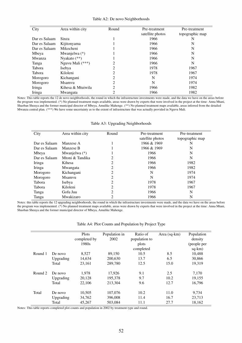
Table A2: De novo Neighborhoods

City Area within city Round Pre-treatmentsatellite photos

Pre-treatmenttopographic map

Dar es Salaam Sinza 1 1966 NDar es Salaam Kijitonyama 1 1966 NDar es Salaam Mikocheni 1 1966 NMbeya Mwanjelwa (*) 1 1966 NMwanza Nyakato (**) 1 1966 NTanga Nguvu Mali (***) 2 1966 NTabora Isebya 2 1978 1967Tabora Kiloleni 2 1978 1967Morogoro Kichangani 2 N 1974Morogoro Msamvu 2 N 1974Iringa Kihesa & Mtuiwila 2 1966 1982Iringa Mwangata 2 1966 1982

Notes: This table reports the 12 de novo neighborhoods, the round in which the infrastructure investments were made, and the data we have on the areas beforethe program was implemented. (*) No planned treatment maps available, areas were drawn by experts that were involved in the project at the time: Anna Mtani,Shaoban Sheuya and the former municipal director of Mbeya, Amulike Mahenge. (**) No planned treatment maps available, areas inferred from the detailedMwanza central plan. (***) We have some uncertainty as to the extent of infrastructure that was actually provided in Nguvu Mali.

Table A3: Upgrading Neighborhoods

City Area within city Round Pre-treatmentsatellite photos

Pre-treatmenttopographic map

Dar es Salaam Manzese A 1 1966 & 1969 NDar es Salaam Manzese B 1 1966 & 1969 NMbeya Mwanjelwa (*) 1 1966 NDar es Salaam Mtoni & Tandika 2 1966 NIringa Kihesa 2 1966 1982Iringa Mwangata 2 1966 1982Morogoro Kichangani 2 N 1974Morogoro Msamvu 2 N 1974Tabora Isebya 2 1978 1967Tabora Kiloleni 2 1978 1967Tanga Gofu Juu 2 1966 NTanga Mwakizaro 2 1966 N

Notes: this table reports the 12 upgrading neighborhoods, the round in which the infrastructure investments were made, and the data we have on the areas beforethe program was implemented. (*) No planned treatment maps available, areas were drawn by experts that were involved in the project at the time: Anna Mtani,Shaoban Sheuya and the former municipal director of Mbeya, Amulike Mahenge.

Table A4: Plot Counts and Population by Project Type

Plotscompleted by

1980s

Population in2002

Ratio ofpopulation to

plotscompleted

Area (sq-km) Populationdensity

(people persq-km)

Round 1 De novo 8,527 89,150 10.5 8.5 10,488Upgrading 14,634 200,630 13.7 6.5 30,866Total 23,161 289,780 12.5 15.0 19,319

Round 2 De novo 1,978 17,926 9.1 2.5 7,170Upgrading 20,128 195,378 9.7 10.2 19,155Total 22,106 213,304 9.6 12.7 16,796

Total De novo 10,505 107,076 10.2 11.0 9,734Upgrading 34,762 396,008 11.4 16.7 23,713Total 45,267 503,084 11.1 27.7 18,162

Notes: This table reports completed plot counts and population in 2002 by treatment type and round.

52

Table A5: Summary Statistics

Imagerydata

(Blocks)

Imagerydata

(Buildings)

TSCP(Blocks)

TSCP(Buildings)

TSCP(Units)

De novo 0.206(0.404)

0.163(0.369)

0.022(0.148)

0.024(0.154)

0.027(0.161)

Upgrading 0.314(0.464)

0.468(0.499)

0.019(0.136)

0.037(0.188)

0.057(0.231)

Control 0.480(0.500)

0.369(0.483)

0.073(0.261)

0.068(0.251)

0.071(0.257)

Mean log building footprint area 4.443(0.596)

4.235(0.848)

4.882(0.650)

4.628(0.696)

4.692(0.724)

Share of buildings with paintedroof 0.155

(0.230)0.155

(0.362)Share of buildings with noneighbor within 1m 0.451

(0.353)0.309

(0.462)Mean similarity of buildingorientation -6.944

(6.203)-6.555(8.301)

Share of buildings with road within10m 0.170

(0.268)0.184

(0.387)Share of buildings with multiplestoreys 0.111

(0.294)0.070

(0.254)0.088

(0.283)

Share of buildings with a good roof 0.945(0.180)

0.944(0.229)

0.952(0.214)

Share of buildings connected toelectricity 0.494

(0.422)0.446

(0.497)0.482

(0.500)

Share of buildings with sewerageor septic tank 0.399

(0.425)0.366

(0.482)0.353

(0.478)

Share of buildings connected towater mains 0.556

(0.417)0.500

(0.500)0.518

(0.500)

Share of buildings with road access 0.674(0.428)

0.617(0.486)

0.655(0.475)

Obs. 21,602 143,343 43,222 119,914 154,734Notes: Summary statistics are estimates of the sample mean and its standard deviation in parentheses. Columns 1-2 display summary statistics for outcomesderived from satellite imagery for all seven Sites and Services cities over the sample of observations with their centroid in either a de novo, upgrading, or controlarea. Columns 3-5 display summary statistics for outcomes derived from TSCP survey data for Mbeya, Mwanza, and Tanga over the whole city sample.Observations are blocks based on an arbitrary grid of 50x50 meters for columns 1 and 3, buildings for columns 2 and 4, and units for column 5. All columnsreport the maximum populated number of observations. Block outcomes are derived from all buildings with a centroid in the block. Blocks that fall betweentwo treatment types are assigned according to where their centroid falls. Variable Good Roof Materials has 3068 fewer observations due to measurement errorin assigning roof type to a building (outlines of the building in Dar es Salaam did not correspond to an actual building on the satellite image). Similarly, LogBuilding Size and Similarity of Orientation have 4 and 14 fewer observations respectively, because of measurement error.

53

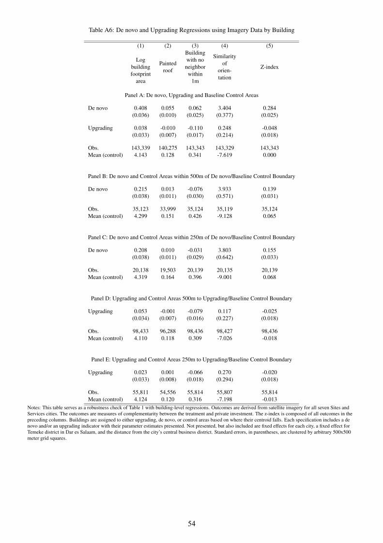
Table A6: De novo and Upgrading Regressions using Imagery Data by Building

(1) (2) (3) (4) (5)

Logbuildingfootprint

area

Paintedroof

Buildingwith no

neighborwithin

1m

Similarityof

orien-tation

Z-index

Panel A: De novo, Upgrading and Baseline Control Areas

De novo 0.408 0.055 0.062 3.404 0.284(0.036) (0.010) (0.025) (0.377) (0.025)

Upgrading 0.038 -0.010 -0.110 0.248 -0.048(0.033) (0.007) (0.017) (0.214) (0.018)

Obs. 143,339 140,275 143,343 143,329 143,343Mean (control) 4.143 0.128 0.341 -7.619 0.000

Panel B: De novo and Control Areas within 500m of De novo/Baseline Control Boundary

De novo 0.215 0.013 -0.076 3.933 0.139(0.038) (0.011) (0.030) (0.571) (0.031)

Obs. 35,123 33,999 35,124 35,119 35,124Mean (control) 4.299 0.151 0.426 -9.128 0.065

Panel C: De novo and Control Areas within 250m of De novo/Baseline Control Boundary

De novo 0.208 0.010 -0.031 3.803 0.155(0.038) (0.011) (0.029) (0.642) (0.033)

Obs. 20,138 19,503 20,139 20,135 20,139Mean (control) 4.319 0.164 0.396 -9.001 0.068

Panel D: Upgrading and Control Areas 500m to Upgrading/Baseline Control Boundary

Upgrading 0.053 -0.001 -0.079 0.117 -0.025(0.034) (0.007) (0.016) (0.227) (0.018)

Obs. 98,433 96,288 98,436 98,427 98,436Mean (control) 4.110 0.118 0.309 -7.026 -0.018

Panel E: Upgrading and Control Areas 250m to Upgrading/Baseline Control Boundary

Upgrading 0.023 0.001 -0.066 0.270 -0.020(0.033) (0.008) (0.018) (0.294) (0.018)

Obs. 55,811 54,556 55,814 55,807 55,814Mean (control) 4.124 0.120 0.316 -7.198 -0.013

Notes: This table serves as a robustness check of Table 1 with building-level regressions. Outcomes are derived from satellite imagery for all seven Sites andServices cities. The outcomes are measures of complementarity between the treatment and private investment. The z-index is composed of all outcomes in thepreceding columns. Buildings are assigned to either upgrading, de novo, or control areas based on where their centroid falls. Each specification includes a denovo and/or an upgrading indicator with their parameter estimates presented. Not presented, but also included are fixed effects for each city, a fixed effect forTemeke district in Dar es Salaam, and the distance from the city’s central business district. Standard errors, in parentheses, are clustered by arbitrary 500x500meter grid squares.

54

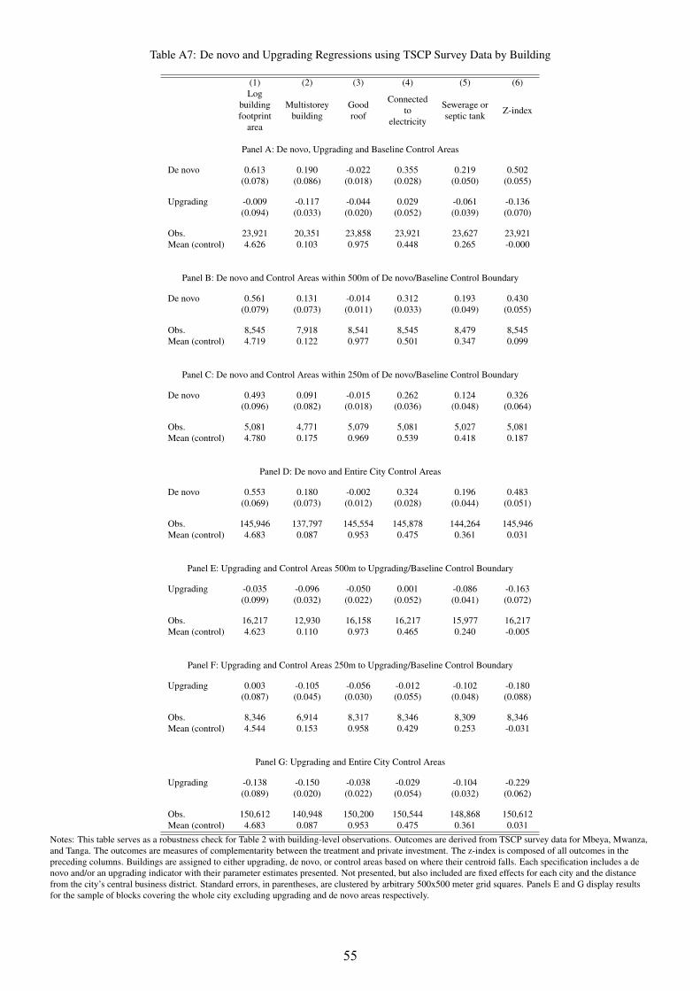
Table A7: De novo and Upgrading Regressions using TSCP Survey Data by Building

(1) (2) (3) (4) (5) (6)Log

buildingfootprint

area

Multistoreybuilding

Goodroof

Connectedto

electricity

Sewerage orseptic tank Z-index

Panel A: De novo, Upgrading and Baseline Control Areas

De novo 0.613 0.190 -0.022 0.355 0.219 0.502(0.078) (0.086) (0.018) (0.028) (0.050) (0.055)

Upgrading -0.009 -0.117 -0.044 0.029 -0.061 -0.136(0.094) (0.033) (0.020) (0.052) (0.039) (0.070)

Obs. 23,921 20,351 23,858 23,921 23,627 23,921Mean (control) 4.626 0.103 0.975 0.448 0.265 -0.000

Panel B: De novo and Control Areas within 500m of De novo/Baseline Control Boundary

De novo 0.561 0.131 -0.014 0.312 0.193 0.430(0.079) (0.073) (0.011) (0.033) (0.049) (0.055)

Obs. 8,545 7,918 8,541 8,545 8,479 8,545Mean (control) 4.719 0.122 0.977 0.501 0.347 0.099

Panel C: De novo and Control Areas within 250m of De novo/Baseline Control Boundary

De novo 0.493 0.091 -0.015 0.262 0.124 0.326(0.096) (0.082) (0.018) (0.036) (0.048) (0.064)

Obs. 5,081 4,771 5,079 5,081 5,027 5,081Mean (control) 4.780 0.175 0.969 0.539 0.418 0.187

Panel D: De novo and Entire City Control Areas

De novo 0.553 0.180 -0.002 0.324 0.196 0.483(0.069) (0.073) (0.012) (0.028) (0.044) (0.051)

Obs. 145,946 137,797 145,554 145,878 144,264 145,946Mean (control) 4.683 0.087 0.953 0.475 0.361 0.031

Panel E: Upgrading and Control Areas 500m to Upgrading/Baseline Control Boundary

Upgrading -0.035 -0.096 -0.050 0.001 -0.086 -0.163(0.099) (0.032) (0.022) (0.052) (0.041) (0.072)

Obs. 16,217 12,930 16,158 16,217 15,977 16,217Mean (control) 4.623 0.110 0.973 0.465 0.240 -0.005

Panel F: Upgrading and Control Areas 250m to Upgrading/Baseline Control Boundary

Upgrading 0.003 -0.105 -0.056 -0.012 -0.102 -0.180(0.087) (0.045) (0.030) (0.055) (0.048) (0.088)

Obs. 8,346 6,914 8,317 8,346 8,309 8,346Mean (control) 4.544 0.153 0.958 0.429 0.253 -0.031

Panel G: Upgrading and Entire City Control Areas

Upgrading -0.138 -0.150 -0.038 -0.029 -0.104 -0.229(0.089) (0.020) (0.022) (0.054) (0.032) (0.062)

Obs. 150,612 140,948 150,200 150,544 148,868 150,612Mean (control) 4.683 0.087 0.953 0.475 0.361 0.031

Notes: This table serves as a robustness check for Table 2 with building-level observations. Outcomes are derived from TSCP survey data for Mbeya, Mwanza,and Tanga. The outcomes are measures of complementarity between the treatment and private investment. The z-index is composed of all outcomes in thepreceding columns. Buildings are assigned to either upgrading, de novo, or control areas based on where their centroid falls. Each specification includes a denovo and/or an upgrading indicator with their parameter estimates presented. Not presented, but also included are fixed effects for each city and the distancefrom the city’s central business district. Standard errors, in parentheses, are clustered by arbitrary 500x500 meter grid squares. Panels E and G display resultsfor the sample of blocks covering the whole city excluding upgrading and de novo areas respectively.

55

Table A8: De novo and Upgrading Regressions using TSCP Survey Data (Weighted by Units per Building) with Owner FullName Fixed Effects

(1) (2) (3) (4) (5) (6)Log

buildingfootprint

area

Multistoreybuilding

Goodroof

Connectedto

electricity

Sewerage orseptic tank

Z-index

Panel A: Baseline Model without Name Fixed Effects (Weighted by Inverse Number of Units in Each Buiding)

De novo 0.520 0.119 0.002 0.357 0.232 0.473(0.062) (0.053) (0.013) (0.027) (0.049) (0.050)

Upgrading -0.035 -0.080 -0.083 -0.029 -0.053 -0.195(0.080) (0.026) (0.032) (0.047) (0.051) (0.081)

Obs. 23,921 20,351 23,858 23,921 23,627 23,921Mean (control) 4.626 0.103 0.975 0.448 0.265 -0.000

Panel B: Owner Last Name Fixed Effects (Weighted by Inverse Number of Units in Each Buiding)

De novo 0.658 0.111 -0.016 0.382 0.250 0.503(0.066) (0.066) (0.014) (0.029) (0.064) (0.054)

Upgrading 0.029 -0.108 -0.058 0.009 -0.033 -0.134(0.075) (0.038) (0.024) (0.046) (0.038) (0.072)

Obs. 11,122 8,698 11,082 11,122 10,899 11,122Mean (control) 4.626 0.103 0.975 0.448 0.265 -0.000

Panel C: Owner Full Name Fixed Effects (Weighted by Inverse Number of Units in Each Buiding)

De novo 0.296 0.134 0.035 0.182 0.109 0.344(0.104) (0.096) (0.038) (0.106) (0.130) (0.145)

Upgrading -0.020 -0.021 -0.013 0.280 0.041 0.086(0.108) (0.043) (0.042) (0.079) (0.085) (0.117)

Obs. 6,493 4,655 6,457 6,493 6,311 6,493Mean (control) 4.626 0.103 0.975 0.448 0.265 -0.000

Notes: This table serves as a robustness check for Table 3 with unit-level observations weighted by the number of units in each building. Outcomes are at thebuilding level and derived from TSCP survey data for Mbeya, Mwanza, and Tanga. The outcomes are measures of complementarity between the treatment andprivate investment. The z-index is composed of all outcomes in the preceding columns. Units are assigned to either upgrading, de novo, or control areas basedon where their building’s centroid falls. Each specification includes a de novo and/or an upgrading indicator with their parameter estimates presented. Notpresented, but also included are fixed effects for each city and the distance from the city’s central business district. Standard errors, in parentheses, are clusteredby arbitrary 500x500 meter grid squares. Panel A displays results for the full sample of units inside de novo, upgrading, and baseline control areas. Panel Bdisplays results adding unit owner last name fixed effects and further restricting the sample by dropping singletons; keeping only last name owners that appearmore than once in the sample. Panel C displays results adding owner full (first and last) name fixed effects and further restricting the sample by droppingsingletons; keeping only full name owners that appear more than once in the sample.

56

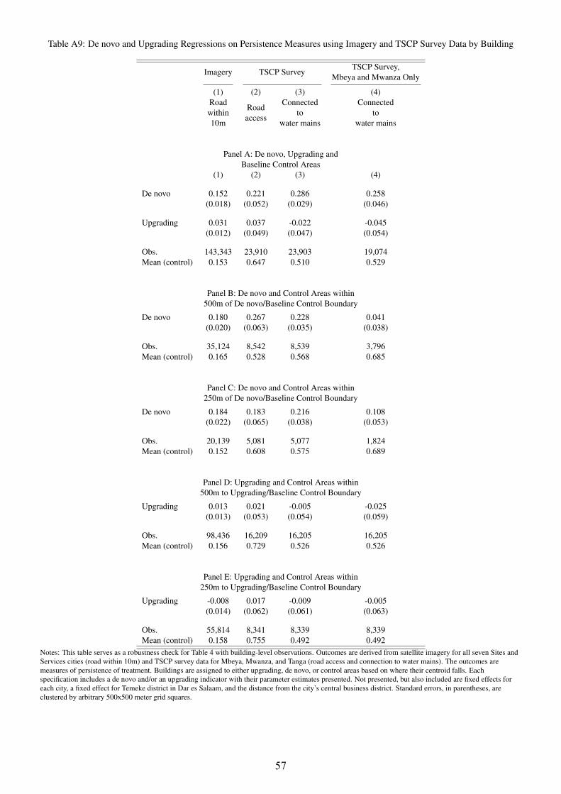
Table A9: De novo and Upgrading Regressions on Persistence Measures using Imagery and TSCP Survey Data by Building

Imagery TSCP SurveyTSCP Survey,

Mbeya and Mwanza Only

(1) (2) (3) (4)Roadwithin10m

Roadaccess

Connectedto

water mains

Connectedto

water mains

Panel A: De novo, Upgrading andBaseline Control Areas

(1) (2) (3) (4)

De novo 0.152 0.221 0.286 0.258(0.018) (0.052) (0.029) (0.046)

Upgrading 0.031 0.037 -0.022 -0.045(0.012) (0.049) (0.047) (0.054)

Obs. 143,343 23,910 23,903 19,074Mean (control) 0.153 0.647 0.510 0.529

Panel B: De novo and Control Areas within500m of De novo/Baseline Control Boundary

De novo 0.180 0.267 0.228 0.041(0.020) (0.063) (0.035) (0.038)

Obs. 35,124 8,542 8,539 3,796Mean (control) 0.165 0.528 0.568 0.685

Panel C: De novo and Control Areas within250m of De novo/Baseline Control Boundary

De novo 0.184 0.183 0.216 0.108(0.022) (0.065) (0.038) (0.053)

Obs. 20,139 5,081 5,077 1,824Mean (control) 0.152 0.608 0.575 0.689

Panel D: Upgrading and Control Areas within500m to Upgrading/Baseline Control Boundary

Upgrading 0.013 0.021 -0.005 -0.025(0.013) (0.053) (0.054) (0.059)

Obs. 98,436 16,209 16,205 16,205Mean (control) 0.156 0.729 0.526 0.526

Panel E: Upgrading and Control Areas within250m to Upgrading/Baseline Control Boundary

Upgrading -0.008 0.017 -0.009 -0.005(0.014) (0.062) (0.061) (0.063)

Obs. 55,814 8,341 8,339 8,339Mean (control) 0.158 0.755 0.492 0.492

Notes: This table serves as a robustness check for Table 4 with building-level observations. Outcomes are derived from satellite imagery for all seven Sites andServices cities (road within 10m) and TSCP survey data for Mbeya, Mwanza, and Tanga (road access and connection to water mains). The outcomes aremeasures of persistence of treatment. Buildings are assigned to either upgrading, de novo, or control areas based on where their centroid falls. Eachspecification includes a de novo and/or an upgrading indicator with their parameter estimates presented. Not presented, but also included are fixed effects foreach city, a fixed effect for Temeke district in Dar es Salaam, and the distance from the city’s central business district. Standard errors, in parentheses, areclustered by arbitrary 500x500 meter grid squares.

57

Table A10: De novo and Upgrading Regressions for Rounds 1 and 2 using Imagery Data by Building

(1) (2) (3) (4) (5) (6)

Logbuildingfootprint

area

Paintedroof

Buildingwith no

neighborwithin

1m

Similarityof

orien-tation

Roadwithin10m

Z-index

De novo 1 0.470 0.074 0.090 3.830 0.167 0.343(0.044) (0.013) (0.031) (0.465) (0.022) (0.029)

De novo 2 0.113 -0.011 -0.082 2.410 0.070 0.047(0.034) (0.007) (0.030) (0.693) (0.024) (0.023)

Upgrading 1 -0.007 -0.005 -0.139 0.684 0.012 -0.061(0.051) (0.011) (0.024) (0.279) (0.015) (0.026)

Upgrading 2 0.088 -0.021 -0.075 -0.432 0.054 -0.041(0.028) (0.006) (0.023) (0.350) (0.018) (0.022)

Obs. 143,339 140,275 143,343 143,329 143,343 143,343Mean (control) 4.143 0.128 0.341 -7.619 0.153 0.000

Notes: This table serves as a robustness check for Table 5 with building-level observations. Outcomes are derived from satellite imagery for all seven Sites andServices cities. The outcomes are measures of complementarity between the treatment and private investment. The z-index is composed of all outcomes in thepreceding columns. Blocks are assigned to either upgrading, de novo, or control areas based on where their centroid falls. Each specification includes de novoround 1, de novo round 2, upgrading round 1, and upgrading round 2 indicators with their parameter estimates presented. Not presented, but also included arefixed effects for each city, a fixed effect for Temeke district in Dar es Salaam, and the distance from the city’s central business district. Standard errors, inparentheses, are clustered by arbitrary 500x500 meter grid squares.

58

Table A11: Program Estimates by City

(1) (2) (3) (4) (5) (6) (7) (8) (9)

Meanlog

buildingfootprint

area

Share ofbuildingswith no

neighborwithin 1m

Meansimilarity

ofbuildingorien-tation

Shareof buildingswith road

within10m

Z-index(including

roads)

Emptyblock

indicator

Share ofarea

built up

Numberof buildings

Dar-es-Salaam × De novo 0.476 0.210 1.166 0.059 0.416 -0.048 -0.034 -3.630(0.074) (0.047) (0.363) (0.027) (0.062) (0.038) (0.019) (0.773)

Iringa × De novo 0.193 0.010 0.374 -0.003 0.047 -0.164 0.069 0.902(0.055) (0.051) (1.557) (0.040) (0.100) (0.081) (0.035) (0.679)

Mbeya × De novo 0.517 -0.061 2.091 0.200 0.274 -0.138 0.132 -2.995(0.087) (0.037) (0.662) (0.028) (0.070) (0.035) (0.033) (1.481)

Morogoro × De novo -0.068 -0.261 0.526 0.006 -0.216 -0.287 0.125 2.575(0.086) (0.060) (1.154) (0.003) (0.054) (0.084) (0.031) (0.601)

Mwanza × De novo 0.265 -0.164 7.326 0.273 0.450 -0.130 0.149 2.043(0.057) (0.026) (0.538) (0.029) (0.041) (0.038) (0.015) (0.469)

Tabora × De novo -0.020 -0.141 2.369 0.033 0.002 -0.339 0.088 2.225(0.053) (0.040) (0.583) (0.033) (0.046) (0.060) (0.018) (0.431)

Tanga × De novo -0.079 -0.048 0.272 0.040 0.009 -0.017 0.016 1.094(0.149) (0.099) (3.397) (0.041) (0.051) (0.118) (0.051) (1.419)

Dar-es-Salaam × Upgrading -0.078 -0.165 -0.055 0.003 -0.146 -0.169 0.134 4.310(0.055) (0.034) (0.230) (0.014) (0.039) (0.029) (0.014) (0.605)

Iringa × Upgrading 0.095 -0.135 2.937 0.059 0.045 -0.279 0.174 3.008(0.054) (0.052) (0.766) (0.037) (0.059) (0.054) (0.028) (0.496)

Mbeya × Upgrading -0.035 -0.169 0.291 0.010 -0.107 -0.086 0.155 4.234(0.107) (0.040) (0.661) (0.018) (0.065) (0.043) (0.040) (1.421)

Morogoro × Upgrading -0.173 -0.337 -3.955 0.020 -0.421 -0.467 0.244 5.598(0.082) (0.050) (1.235) (0.010) (0.061) (0.053) (0.035) (0.613)

Tabora × Upgrading -0.090 -0.113 -1.268 0.042 -0.109 -0.357 0.102 2.985(0.059) (0.027) (0.701) (0.027) (0.042) (0.062) (0.014) (0.458)

Tanga × Upgrading -0.227 0.021 -2.440 -0.049 -0.185 -0.233 0.090 3.392(0.063) (0.054) (1.036) (0.034) (0.036) (0.071) (0.045) (1.247)

Obs. 17,682 17,682 17,682 17,682 17,682 21,602 21,602 21,602Mean (control) 4.392 0.502 -8.001 0.154 -0.000 0.288 0.184 5.066

Notes: This table serves as a robustness check of Table 1 breaking down treatment effects for each city. Regressions of block level observations with outcomesderived from satellite imagery for all seven Sites and Services cities. The outcomes are measures of complementarity between the treatment and privateinvestment. Each observation is a block based on an arbitrary grid of 50x50 meters. Outcomes are derived from the set of buildings with a centroid in the block.The z-index is composed of all outcomes in the preceding columns. Blocks are assigned to either upgrading, de novo, or control areas based on where theircentroid falls. Each specification includes de novo by city and upgrading by city indicators with their parameter estimates presented. Not presented, but alsoincluded are a fixed effect for Temeke district in Dar es Salaam, and the distance from the city’s central business district. Standard errors, in parentheses, areclustered by arbitrary 500x500 meter grid squares.

59

Table A12: De novo and Upgrading Population Weighted Regressions of Education Using 2012 Census Data

Adult Heads of Household All Adults

(1) (2) (3) (4) (5) (6)

Years ofschooling

Exactlyprimaryschool

More thanprimaryschool

Years ofschooling

Exactlyprimaryschool

More thanprimaryschool

Panel A: Denovo, Upgrading and Control

De novo 2.087 -0.211 0.257 1.821 -0.180 0.222(0.247) (0.028) (0.031) (0.209) (0.023) (0.027)

Upgrading -0.446 0.004 -0.040 -0.342 0.002 -0.031(0.207) (0.022) (0.026) (0.183) (0.021) (0.024)

Observations 2,520 2,520 2,520 2,520 2,520 2,520Mean (control) 8.320 0.532 0.352 8.509 0.515 0.378

Panel B: Denovo, Upgrading and Entire City Control Areas

De novo 2.091 -0.224 0.258 1.830 -0.194 0.223(0.179) (0.026) (0.025) (0.136) (0.018) (0.018)

Upgrading -0.613 0.043 -0.069 -0.612 0.054 -0.075(0.078) (0.009) (0.010) (0.076) (0.007) (0.009)

Observations 18,552 18,552 18,552 18,553 18,553 18,553Mean (control) 8.451 0.523 0.365 8.592 0.506 0.389

Notes: This table serves as a robustness check of Table 6 using population weighted observations. Regressions of cut Enumeration Area (EA) level observationswith outcomes derived from Tanzania 2012 Census microdata for all seven Sites and Services cities. The outcomes are measures of sorting into the treatmentand control areas. Each observation is a cut EA of varying size. Outcomes are the EA mean over the set of either heads of household at least 18 years old(columns 1-3) or all adults at least 18 years old (columns 4-6) enumerated in the EA. Cut EAs are assigned to upgrading, de novo, and/or control areas if morethan 5% of the cut EA lies inside the respective area. Analytic weights for the cut EA observations used in the regression are based on the proportion of the EAarea that lies inside each treatment or control area, multiplied by the number of people (adult head of households for columns 1-3, adults for columns 4-6)contributing to the EA mean of the outcome variable. Each specification includes a de novo and an upgrading indicator with their parameter estimatespresented. Not presented, but also included are fixed effects for each city, fixed effects for Temeke and Ilala districts in Dar es Salaam, and fixed effects for thedistance from the city’s central business district. Standard errors, in parentheses, are clustered by arbitrary 500x500 meter grid squares. Panel B displays resultsfor the sample of EAs covering the whole city, which means all urban EAs within the same administrative area as the relevant treatment areas.

60

Table A13: De novo and Upgrading Regressions of Building Outcomes on EA level

(1) (2) (3) (4) (5)

Meanlog

buildingfootprint

area

Share ofbuildings

withpainted

roof

Share ofbuildingswith no

neighborwithin 1m

Meansimilarity

ofbuildingorien-tation

Shareof buildingswith road

within10m

Panel A: De novo, Upgrading and Control, not Controlling for Years of Schooling

De novo 0.360 0.054 0.041 2.779 0.099(0.069) (0.018) (0.043) (0.347) (0.022)

Upgrading 0.118 -0.027 -0.010 -0.325 0.032(0.041) (0.012) (0.029) (0.324) (0.009)

Observations 2,454 2,454 2,454 2,454 2,454Mean (control) 4.269 0.169 0.397 -6.742 0.117

Panel B: Controlling for Years of Schooling of Household Head

De novo 0.290 0.039 0.012 2.545 0.092(0.071) (0.017) (0.044) (0.350) (0.023)

Upgrading 0.130 -0.024 -0.006 -0.287 0.033(0.037) (0.011) (0.028) (0.315) (0.009)

Years of schooling 0.038 0.008 0.016 0.128 0.004(0.007) (0.002) (0.004) (0.044) (0.002)

Observations 2,454 2,454 2,454 2,454 2,454Mean (control) 4.269 0.169 0.397 -6.742 0.117

Notes: This table serves as a robustness check of Table 1 using cut EA observations and demographic controls. Regressions of cut Enumeration Area (EA) levelobservations with outcomes derived from satellite imagery, for all seven Sites and Services cities. Each observation is a cut EA of varying size, with the mean ofthe building level indicators taken over all the buildings present in the cut EA. Cut EAs are assigned to upgrading, de novo, and/or control areas if more than 5%of the cut EA lies inside the respective area. Each specification includes de novo and upgrading indicators with their parameter estimates presented, while inPanel B we also control for years of schooling. The years of schooling variable is derived from the 2012 Tanzanian census data by taking the EA mean of allenumerated adult heads of household. Not presented, but also included are fixed effects for each city, fixed effects for Temeke and Ilala districts in Dar esSalaam, and fixed effects for the distance from the city’s central business district. Standard errors, in parentheses, are clustered by arbitrary 500x500 meter gridsquares.

61

Table A14. Details on the Selection of Control Areas by City

Dar esSalaam

• Sources: the 1974 (World Bank 1974a) and 1977 (World Bank 1977b) project proposal maps.• De novo and upgrading: the 1974 map is used to trace areas in the north of Dar es Salaam (KinondoniMunicipality), and the 1977 map is used in the south of Dar es Salaam (Temeke municipality).• Exclusions: the 1974 map is used to exclude areas in Kinondoni where we identify previously establishedresidential areas and land reserved for special institutions and industry. The 1977 map is used to excludeareas in Temeke where there are low density residential areas and special institutions.

Iringa • Sources: the 1977 project proposal map (World Bank 1977b), and a 1978 topographic map (Directorateof Overseas Surveys, 2015).• De novo and upgrading: the 1977 project proposal map is used to trace areas.• Exclusions: the 1977 project proposal map is used to exclude industrial and established residential areaseast of Mwangata. The 1978 topographic map is used to exclude already developed areas west and east ofMwangata, and also north, south and east of Kihesa. Additionally, north of Mwangata is excluded becauseof a power plant.

Mbeya• Sources: a 1966 satellite image (United States Geological Survey, 2015), and drawings by experts onthe Sites and Services projects in Mbeya. Those experts are Shaoban Sheuya, Anna Mtani, and AmulikeMahenge and were all interviewed by the authors in Dar es Salaam, June 30, 2016.• De novo and upgrading: the drawings from our experts were used to trace areas.• Exclusions: the 1966 satellite image is used to exclude areas with shops along the highway south east ofMwanjelwa, already developed areas north west of Mwanjelwa, and the airport.

Morogoro • Sources: the 1977 project proposal map (World Bank 1977b), and a 1974 topographic map (Directorateof Overseas Surveys, 2015).• De novo and upgrading: the 1977 project proposal map is used to trace areas.• Exclusions: the 1977 project proposal map is used to exclude a large industrial area south west of Msamvuand a large previously developed area to the south of Msamvu. The 1974 topographic map is used toexclude a previously developed area south of Kichangani, and to confirm the exclusions from the 1977project proposal map.

Mwanza • Sources: a 1973 cadastral map (Mwanza City Municipality, 1973).• De novo: the cadastral map is used to trace areas, it delineates all surveyed plots and so contains a fewthat are outside of the actual Sites and Services treatment. We include plots that are small (288m2 is theknown treated plot area) and recorded with a plot number, and community buildings. We do not includeplots that are large or that are small but do not have a recorded plot number.• Exclusions: the cadastral map is used to exclude areas with large plots or plots without a recorded number.Also excluded are previously developed areas along the road in the south east of Mwanza, as well as areasto the north that are off of the map.

Tabora • Sources: the 1977 project proposal map (World Bank 1977b), a 1967 topographic map (Directorate ofOverseas Surveys, 2015), and 1978 aerial imagery (Directorate of Overseas Surveys, 2015).• De novo and upgrading: the 1977 project proposal map is used to trace areas.• Exclusions: the project proposal map is used to excluded previously built areas to the west and south westof the Kiloleni. The 1967 topographic map is used to exclude an industrial area to the south of Isebeya inbetween the two of upgrading area. The 1978 aerial image is used to confirm the exclusions.

Tanga • Sources: the 1977 project proposal map (World Bank 1977b), and a 1966 satellite image (United StatesGeological Survey, 2015).• De novo and upgrading: the 1977 project proposal map is used to trace areas.• Exclusions from control areas: the 1966 satellite image is used to exclude already developed areas south,south west, north and east of Gofu Juu and east of Mwakizaro. The 1977 project proposal map is used toexclude industrial area between Gofu Juu and Mwakizaro.

Notes: This table explains what imagery and maps were used to (a) delineate the de novo and upgrading areas, and (b) create exclusion areas (ie. areas to beexcluded from the control areas) among areas that are within 500 meters of Sites and Services, as explained in the Data Appendix. Sources are all georeferencedmaps of the city in question. Almost all areas in the studied cities were covered by these maps, with minor exceptions in the western areas of Tabora, and northof the northern treatment area (Kihesa neighborhood) in Iringa.

62

Table A15. Description of Variables Derived from Imagery Data

Variable label Definition

Building-level and grid-cell outcomes

Log building footprint area Calculated directly for the shape file (calculated as a direct measure forthe building, or a sample average of that measure for each grid-cell).

Painted roof Indicator for painted or clay as opposed to tin or rusted tin (an indicatorfor the building or a share of buildings with painted roofs for each grid-cell).

Building with no neighborwithin 1m

Distance to the nearest building calculated using the nearest two pointsno the border of the building outlines is less than or equal to 1m (calcu-lated as an indicator for the building or a share of buildings with nearestbuilding 1 m away for each grid-cell).

Similarity of orientation Calculated using the main axis of the minimum bounding box that con-tains each building. We then calculated the difference in orientation be-tween each building and its neighboring building, modulo 90 degrees,with more similar orientations representing a more regular layout (anindicator for the building or a sample average for each grid-cell).

Z-index Kling et al. 2007; Banerjee et al. 2014. We integrate all “good” vari-ables into one index. We subtract the mean in the control group and di-vide the result by the standard deviation in the control group. Then wecreate the index by taking a simple average of the normalized variables(a measure for the building or a sample average for each grid-cell).

Road within 10m An indicator that the distance form the boundary of the building to thenearest roads is no more than 10m).

Distance to the CBD The CBD for each city is the centroid of the most lit pixel in 1992 fromthe NOAA “Average Visible and Stable Lights, Cloud Free Coverage”dataset. The distance to the CBD is calculated from the centroids ofeach building or grid-cell.

Grid-cell outcomes only

Empty Indicator for a grid cell that has no buildings.

Share of area built Share of the area of the grid cell that is built.

Number of buildings per50x50m

Count of buildings in a grid cell.

Note: this table describes the variables derived from Worldview and Ramani Huria building shapefiles.

63

Table A16. Description of TSCP variables and how they are created

Variable label Definition

Building-level outcomes

Connected to electricity Indicator for whether a building is connected to electricity.

Sewerage or septic tank Indicator for good sanitation, i.e. having sewerage or a septic tank asopposed to an alternative of pit latrine, no sanitation at all, or other.

Good roof Indicator for roof being made of concrete, metal sheets, clay tiles orcement tiles as opposed to an alternative of grass/palm, asbestos, timberor other. This is a different measure from the ”Painted roof” variable inTable A15.

Multistorey building Indicator for one or more storeys above the ground floor.

Z-index Kling et al. 2007; Banerjee et al. 2014. We integrate all “good” vari-ables into one index. We subtract the mean in the control group anddivide the result by the standard deviation in the control group. Thenwe create the index by taking a simple average of the normalized vari-ables.

Connected to water mains Indicator for good water supply (metered/mains as opposed to borehole;stand tap; river; rain; water trucks; or other/none).

Road access Indicator for access to tarmac; gravel; or earth road.

Note: this table describes the variables the we derived from TSCP building data.

64

Table A17. Description of Variables from Tanzanian Census 2012

Variable label Definition

Years of schooling How many years of schooling the respondent (adult or head of house-hold adult) has obtained. Missing values in the microdata are coded as 0since there was no category for ”Never attended school”, and since themissing values were found to match reasonably well with the propor-tion of people with no schooling in the IPUMS 2012 Tanzanian Censusdata (which does not, however, have low level geographical identifiers).Moreover, the proportion of missing values in the microdata increasedwith age and with gender and age, which corresponds to the pattern ofpeople lacking any schooling in Tanzania. Respondents with Trainingafter primary school/Pre-secondary school or Training after secondaryschool are coded as 8 or 12 years respectively, i.e. one more year thanprimary or secondary schooling. Respondents with university educa-tion, are coded as 15, i.e. one more year than the maximum number ofsecondary schooling.

Exactly primary school Binary indicator that takes the value 1 if the respondent (adult or headof household adult) has completed exactly 7 years of schooling, 0 oth-erwise. Missing values coded as 0 as in the variable above.

More than primary school Binary indicator that takes the value 1 if the respondent has completedmore than 7 years of schooling, 0 otherwise. Missing values coded as 0as in the variables above.

Note: this table describes the variables derived from the Tanzanian Census 2012 microdata.

65

Spatial Economics Research Centre (SERC)London School of EconomicsHoughton StreetLondon WC2A 2AE

Web: www.spatialeconomics.ac.uk