Planck intermediate results. XVII. Emission of dust in the diffuse interstellar medium from the far-infared to microwave frequencies

A&A 566, A55 (2014)DOI: 10.1051/0004-6361/201323270c© ESO 2014

Astronomy&

Astrophysics

Planck intermediate resultsXVII. Emission of dust in the diffuse interstellar medium from the far-infrared

to microwave frequencies�

Planck Collaboration: A. Abergel56, P. A. R. Ade79, N. Aghanim56, M. I. R. Alves56, G. Aniano56, M. Arnaud68, M. Ashdown65,7, J. Aumont56,C. Baccigalupi78, A. J. Banday81,11, R. B. Barreiro62, J. G. Bartlett1,63, E. Battaner83, K. Benabed57,80, A. Benoit-Lévy24,57,80, J.-P. Bernard81,11,

M. Bersanelli33,48, P. Bielewicz81,11,78, J. Bobin68, A. Bonaldi64, J. R. Bond10, F. R. Bouchet57,80, F. Boulanger56,��, C. Burigana47,31,J.-F. Cardoso69,1,57, A. Catalano70,67, A. Chamballu68,16,56, H. C. Chiang27,8, P. R. Christensen75,36, D. L. Clements53, S. Colombi57,80,

L. P. L. Colombo23,63, F. Couchot66, B. P. Crill63,76, F. Cuttaia47, L. Danese78, R. J. Davis64, P. de Bernardis32, A. de Rosa47, G. de Zotti43,78,J. Delabrouille1, F.-X. Désert51, C. Dickinson64, J. M. Diego62, H. Dole56,55, S. Donzelli48, O. Doré63,12, M. Douspis56, X. Dupac39,

G. Efstathiou59, T. A. Enßlin73, H. K. Eriksen60, E. Falgarone67, F. Finelli47,49, O. Forni81,11, M. Frailis45, E. Franceschi47, S. Galeotta45,K. Ganga1, T. Ghosh56, M. Giard81,11, Y. Giraud-Héraud1, J. González-Nuevo62,78, K. M. Górski63,84, A. Gregorio34,45, A. Gruppuso47,

V. Guillet56, F. K. Hansen60, D. Harrison59,65, G. Helou12, S. Henrot-Versillé66, C. Hernández-Monteagudo13,73 , D. Herranz62, S. R. Hildebrandt12,E. Hivon57,80, M. Hobson7, W. A. Holmes63, A. Hornstrup17, W. Hovest73, K. M. Huffenberger25, A. H. Jaffe53, T. R. Jaffe81,11, G. Joncas19,A. Jones56, W. C. Jones27, M. Juvela26, P. Kalberla6, E. Keihänen26, J. Kerp6, R. Keskitalo22,14, T. S. Kisner72, R. Kneissl38,9, J. Knoche73,

M. Kunz18,56,3, H. Kurki-Suonio26,41, G. Lagache56, A. Lähteenmäki2,41, J.-M. Lamarre67, A. Lasenby7,65, C. R. Lawrence63, R. Leonardi39,F. Levrier67, M. Liguori30, P. B. Lilje60, M. Linden-Vørnle17, M. López-Caniego62, P. M. Lubin28, J. F. Macías-Pérez70, B. Maffei64,D. Maino33,48, N. Mandolesi47,5,31, M. Maris45, D. J. Marshall68, P. G. Martin10, E. Martínez-González62, S. Masi32, M. Massardi46,

S. Matarrese30, P. Mazzotta35, A. Melchiorri32,50, L. Mendes39, A. Mennella33,48, M. Migliaccio59,65, S. Mitra52,63, M.-A. Miville-Deschênes56,10,A. Moneti57, L. Montier81,11, G. Morgante47, D. Mortlock53, D. Munshi79, J. A. Murphy74, P. Naselsky75,36, F. Nati32, P. Natoli31,4,47, F. Noviello64,D. Novikov53, I. Novikov75, C. A. Oxborrow17, L. Pagano32,50, F. Pajot56, D. Paoletti47,49, F. Pasian45, O. Perdereau66, L. Perotto70, F. Perrotta78,

F. Piacentini32, M. Piat1, E. Pierpaoli23, D. Pietrobon63, S. Plaszczynski66, E. Pointecouteau81,11, G. Polenta4,44, N. Ponthieu56,51, L. Popa58,G. W. Pratt68, S. Prunet57,80, J.-L. Puget56, J. P. Rachen21,73, W. T. Reach82, R. Rebolo61,15,37, M. Reinecke73, M. Remazeilles64,56,1, C. Renault70,

S. Ricciardi47, T. Riller73, I. Ristorcelli81,11, G. Rocha63,12, C. Rosset1, G. Roudier1,67,63, B. Rusholme54, M. Sandri47, G. Savini77, L. D. Spencer79,J.-L. Starck68, F. Sureau68, D. Sutton59,65, A.-S. Suur-Uski26,41, J.-F. Sygnet57, J. A. Tauber40, L. Terenzi47, L. Toffolatti20,62, M. Tomasi48,

M. Tristram66, M. Tucci18,66, G. Umana42, L. Valenziano47, J. Valiviita41,26,60, B. Van Tent71, L. Verstraete56, P. Vielva62, F. Villa47, L. A. Wade63,B. D. Wandelt57,80,29, B. Winkel6, D. Yvon16, A. Zacchei45, and A. Zonca28

(Affiliations can be found after the references)

Received 18 December 2013 / Accepted 29 January 2014

ABSTRACT

The dust-H i correlation is used to characterize the emission properties of dust in the diffuse interstellar medium (ISM) from far infrared wave-lengths to microwave frequencies. The field of this investigation encompasses the part of the southern sky best suited to study the cosmic infraredand microwave backgrounds. We cross-correlate sky maps from Planck, the Wilkinson Microwave Anisotropy Probe (WMAP), and the diffuseinfrared background experiment (DIRBE), at 17 frequencies from 23 to 3000 GHz, with the Parkes survey of the 21 cm line emission of neu-tral atomic hydrogen, over a contiguous area of 7500 deg2 centred on the southern Galactic pole. We present a general methodology to studythe dust-H i correlation over the sky, including simulations to quantify uncertainties. Our analysis yields four specific results. (1) We map thetemperature, submillimetre emissivity, and opacity of the dust per H-atom. The dust temperature is observed to be anti-correlated with the dustemissivity and opacity. We interpret this result as evidence of dust evolution within the diffuse ISM. The mean dust opacity is measured to be(7.1 ± 0.6) × 10−27 cm2 H−1 × (ν/353 GHz)1.53± 0.03 for 100 ≤ ν ≤ 353 GHz. This is a reference value to estimate hydrogen column densitiesfrom dust emission at submillimetre and millimetre wavelengths. (2) We map the spectral index βmm of dust emission at millimetre wavelengths(defined here as ν ≤ 353 GHz), and find it to be remarkably constant at βmm = 1.51 ± 0.13. We compare it with the far infrared spectral index βFIR

derived from greybody fits at higher frequencies, and find a systematic difference, βmm−βFIR = −0.15, which suggests that the dust spectral energydistribution (SED) flattens at ν ≤ 353 GHz. (3) We present spectral fits of the microwave emission correlated with H i from 23 to 353 GHz, whichseparate dust and anomalous microwave emission (AME). We show that the flattening of the dust SED can be accounted for with an additionalcomponent with a blackbody spectrum. This additional component, which accounts for (26 ± 6)% of the dust emission at 100 GHz, could repre-sent magnetic dipole emission. Alternatively, it could account for an increasing contribution of carbon dust, or a flattening of the emissivity ofamorphous silicates, at millimetre wavelengths. These interpretations make different predictions for the dust polarization SED. (4) We analyse theresiduals of the dust-H i correlation. We identify a Galactic contribution to these residuals, which we model with variations of the dust emissivityon angular scales smaller than that of our correlation analysis. This model of the residuals is used to quantify uncertainties of the CIB powerspectrum in a companion Planck paper.

Key words. dust, extinction – submillimeter: ISM – local insterstellar matter – infrared: diffuse background – cosmic background radiation

� Appendices are available in electronic form at http://www.aanda.org�� Corresponding author: F. Boulanger, e-mail: [email protected]

Article published by EDP Sciences A55, page 1 of 23

A&A 566, A55 (2014)

1. Introduction

Understanding interstellar dust is a major challenge in astro-physics related to physical and chemical processes in interstel-lar space. The composition of interstellar dust reflects the pro-cesses that contribute to breaking down and rebuilding grainsover timescales much shorter than that of the injection of newlyformed circumstellar or supernova dust. While there is wideconsensus on this view, the composition of interstellar dust andthe processes that drive its evolution are still poorly understood(Zhukovska et al. 2008; Draine 2009; Jones & Nuth 2011).Observations of dust emission are essential in constraining thenature of interstellar grains and their size distribution.

The Planck1 all-sky survey has opened a new era in duststudies by extending to submillimetre wavelengths and mi-crowave frequencies the detailed mapping of the interstellar dustemission provided by past infrared space missions. For the firsttime we have the sensitivity to map the long wavelength emis-sion of dust in the diffuse interstellar medium (ISM). Large dustgrains (size >10 nm) dominate the dust mass. Far from lumi-nous stars, the grains are cold (10–20 K) so that a significantfraction of their emission is over the Planck frequency range.Dipolar emission from small, rapidly spinning, dust particles isan additional emission component accounting for the so-calledanomalous microwave emission (AME) revealed by observa-tions of the cosmic microwave background (CMB) (e.g. Leitchet al. 1997; Banday et al. 2003; Davies et al. 2006; Ghosh et al.2012; Planck Collaboration XX 2011). Magnetic dipole radia-tion from thermal fluctuations in magnetic nano-particles mayalso be a significant emission component over the frequencyrange relevant to CMB studies (Draine & Lazarian 1999; Draine& Hensley 2013), a possibility that has yet to be tested.

The separation of the dust emission from anisotropies ofthe cosmic infrared background (CIB) and the CMB is a diffi-culty for both dust and background studies. The dust-gas corre-lation provides a means to separate these emission componentsfrom an astrophysics perspective, complementary to mathemat-ical component separation methods (Planck Collaboration XII2014). At high Galactic latitudes, the dust emission is known tobe correlated with the 21 cm line emission from neutral atomichydrogen (Boulanger & Perault 1988). This correlation hasbeen used to separate the dust emission from CIB anisotropiesand characterize the emission properties of dust in the diffuseISM using data from the cosmic background explorer (COBE,Boulanger et al. 1996; Dwek et al. 1997; Arendt et al. 1998),the Wilkinson Microwave Anisotropy Probe (WMAP, Lagache2003), and Planck (Planck Collaboration XXIV 2011). Theresidual maps obtained after subtraction of the dust emissioncorrelated with H i have been used successfully to study CIBanisotropies (Puget et al. 1996; Fixsen et al. 1998; Hauser et al.1998; Planck Collaboration XVIII 2011). The correlation analy-sis also yields the spectral energy distribution (SED) of the dustemission normalized per unit hydrogen column density, whichis an essential input to dust models, and a prerequisite for deter-mining the dust temperature and opacity (i.e. the optical depthper hydrogen atom).

The COBE satellite provided the first data on the thermalemission from large dust grains at long wavelengths. These data

1 Planck (http://www.esa.int/Planck) is a project of theEuropean Space Agency (ESA) with instruments provided by two sci-entific consortia funded by ESA member states (in particular the leadcountries France and Italy), with contributions from NASA (USA) andtelescope reflectors provided by a collaboration between ESA and a sci-entific consortium led and funded by Denmark.

were used to define the dust models of Draine & Li (2007),Compiègne et al. (2011) and Siebenmorgen et al. (2014), andthe analytical fit proposed by Finkbeiner et al. (1999), whichhas been widely used by the CMB community to extrapolatethe IRAS all-sky survey to microwave frequencies. Today thePlanck data allow us to characterize the dust emission at mil-limetre wavelengths directly from observations. A first analy-sis of the correlation between Planck and H i observations waspresented in Planck Collaboration XXIV (2011). In that study,the IRAS 100 μm and the 857, 545, and 353 GHz Planck mapswere correlated with H i observations made with the Green BankTelescope (GBT) for a set of fields sampling a range of H i col-umn densities. We extend this early work to microwave frequen-cies, and to a total sky area more than an order of magnitudehigher.

The goal of this paper is to characterize the emission prop-erties of dust in the diffuse ISM, from far infrared to microwavefrequencies, for dust, CIB, and CMB studies. We achieve this bycross-correlating the Planck data with atomic hydrogen emissionsurveyed over the southern sky with the Parkes telescope (theGalactic All Sky Survey, hereafter GASS; McClure-Griffithset al. 2009; Kalberla et al. 2010). We focus on the southernGalactic polar cap (b < −25◦) where the dust-gas correlationis most easily characterized using H i data because the fractionof the sky with significant H2 column density is low (Gillmonet al. 2006). This is also the cleanest part of the southern sky forCIB and CMB studies.

The paper is organized as follows. We start by presenting thePlanck and the ancillary data from the COBE diffuse infraredbackground experiment (DIRBE) and WMAP that we are corre-lating with the H i GASS survey (Sect. 2). The methodology wefollow to quantify the dust-gas correlation is described in Sect. 3.We use the results from the correlation analysis to characterizethe variations of the dust emission properties across the southernGalactic polar cap in Sect. 4 and determine the spectral indexof the thermal dust emission from submm to millimetre wave-lengths in Sect. 5. In Sect. 6, we present the mean SED of dustfrom far infrared to millimetre wavelengths, and a comparisonwith models of the thermal dust emission. Section 7 focuses onthe SED of the H i correlated emission at microwave frequen-cies, which we quantify and model over the full spectral rangerelevant to CMB studies from 23 to 353 GHz. The main resultsof the paper are summarized in Sect. 8. The paper contains fourappendices where we detail specific aspects of the data analysis.In Appendix A, we describe how maps of dust emission are builtfrom the results of the H i correlation analysis. We explain howwe separate dust and CMB emission at microwave frequencies inAppendix B. We detail how we quantify the uncertainties of theresults of the dust-H i correlation in Appendix C. Appendix Dpresents simulations of the dust emission that we use to quantifyuncertainties.

2. Data sets

In this section, we introduce the Planck, H i, and ancillary skymaps we use in the paper.

2.1. Planck data

Planck is the third generation space mission to characterize theanisotropies of the CMB. It observed the sky in nine frequencybands from 30 to 857 GHz with an angular resolution from33′ to 5′ (Planck Collaboration I 2014). The Low FrequencyInstrument (LFI, Mandolesi et al. 2010; Bersanelli et al. 2010;Mennella et al. 2010) observed the 30, 44, and 70 GHz bands

A55, page 2 of 23

Planck Collaboration: Dust emission from the diffuse interstellar medium

0.0 4.5

[MJy sr-1]

-180

-150

-120

-90

-60

-30

0

30

60

90

120

150

-60

-30

0

0.0 10.0

[1020 cm-2]

-180

-150

-120

-90

-60

-30

0

30

60

90

120

150

-60

-30

0

Fig. 1. Left: Planck map at 857 GHz over the area where we have H i data from the GASS survey. The center of the orthographic projection is thesouthern Galactic pole. Galactic longitudes and latitudes are marked by lines and circles, respectively. The Planck image has been smoothed to the16′ resolution of the GASS NHI map. Right: GASS NHI map of Galactic disk emission, obtained by integrating over the velocity range defined byGalactic rotation (Sect. 2.2.2).

with amplifiers cooled to 20 K. The High Frequency Instrument(HFI, Lamarre et al. 2010) observed the 100, 143, 217, 353,545, and 857 GHz bands with bolometers cooled to 0.1 K. Inthis paper, we use the nine Planck frequency maps made fromthe first 15.5 months of the mission (Planck Collaboration I2014) in HEALPix format2. Maps at 70 GHz and below areat Nside = 1024 (pixel size 3.′4); those at 100 GHz and aboveare at Nside = 2048 (1.′7). We refer to previous Planck publi-cations for the data processing, map-making, photometric cali-bration, and photometric uncertainties (Planck Collaboration II2014; Planck Collaboration VI 2014; Planck Collaboration V2014; Planck Collaboration VIII 2014). At HFI frequencies,we analyse maps produced both with and without subtractionof the zodiacal emission (Planck Collaboration XIV 2014). Toquantify uncertainties associated with noise, we use maps madefrom the first and second halves of each stable pointing period(Planck Collaboration VI 2014).

As an example, Fig. 1 shows the 857 GHz map for the areaof the H i GASS survey.

2.2. The GASS H I survey

In this section we explain how we produce the column densitymap of Galactic H i gas that we will use as a spatial template inour dust-gas correlation analysis.

2.2.1. H I observations

We make use of data from the GASS H i survey obtained withthe Parkes telescope (McClure-Griffiths et al. 2009). The 21 cmline emission was mapped over the southern sky (δ < 1◦)with 14.′5 FWHM angular resolution and a velocity resolutionof 1 km s−1. At high Galactic latitudes, the average noise for in-dividual emission-free channel maps is 50 mK (1σ). GASS is

2 Górski et al. (2005), http://healpix.sf.net

the most sensitive, highest angular resolution survey of GalacticH i emission over the southern sky. We use data corrected forinstrumental effects, stray radiation, and radio-frequency inter-ference from Kalberla et al. (2010).

Maps of H i emission integrated over velocities were gener-ated from spectra in the 3D data cube. To minimize uncertaintiesfrom instrumental noise and to eliminate residual instrumentalproblems we do not integrate the emission over all velocities.The problem is that weak systematic biases over a large num-ber of channels can add up to a significant error. We select thechannels on a smoothed data cube to ensure that weak emissionaround H i clouds is not affected. Specifically, we calculate asecond data cube smoothed to angular and velocity resolutionsof 30′ and 8 km s−1. Velocity channels where the emission inthis smoothed data cube is below a 5σ level of 30 mK are notused in the integration. This brightness threshold is applied toeach smoothed spectrum to define the velocity ranges, not nec-essarily contiguous, over which to integrate the signal in the full-resolution data cube. The impact on the HI column density mapof the selection of channels is small and noticeable only in theregions of lowest column densities. The magnitude of the differ-ence between maps produced with and without the 5σ selectionof the channels is a few 1018 H cm−2. This small difference is notcritical for our analysis.

2.2.2. Separation of H I emission from the Galaxyand Magellanic Stream

The southern polar cap contains Galactic H i emission with typ-ical column densities NHI from one to a few times 1020 cm−2,plus a significant contribution from the Magellanic Stream (MS;Nidever et al. 2008). We need to separate the Galactic andMS gas because the dust-to-gas mass ratio of the low metallicityMS gas is lower than that of the Galactic H i.

A55, page 3 of 23

A&A 566, A55 (2014)

0.0 1.0

[1020 cm-2]

-180

-150

-120

-90

-60

-30

0

30

60

90

120

150

-60

-30

0

0.0 1.0

[1020 cm-2]

-180

-150

-120

-90

-60

-30

0

30

60

90

120

150

-60

-30

0

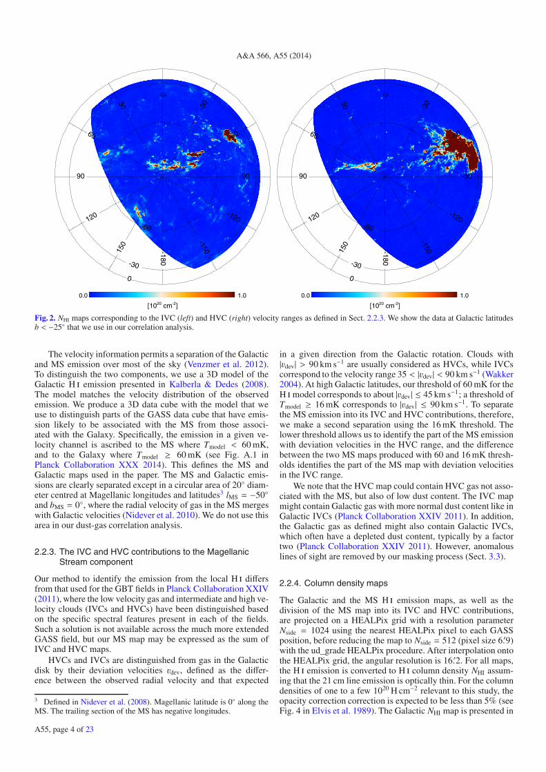
Fig. 2. NHI maps corresponding to the IVC (left) and HVC (right) velocity ranges as defined in Sect. 2.2.3. We show the data at Galactic latitudesb < −25◦ that we use in our correlation analysis.

The velocity information permits a separation of the Galacticand MS emission over most of the sky (Venzmer et al. 2012).To distinguish the two components, we use a 3D model of theGalactic H i emission presented in Kalberla & Dedes (2008).The model matches the velocity distribution of the observedemission. We produce a 3D data cube with the model that weuse to distinguish parts of the GASS data cube that have emis-sion likely to be associated with the MS from those associ-ated with the Galaxy. Specifically, the emission in a given ve-locity channel is ascribed to the MS where Tmodel < 60 mK,and to the Galaxy where Tmodel ≥ 60 mK (see Fig. A.1 inPlanck Collaboration XXX 2014). This defines the MS andGalactic maps used in the paper. The MS and Galactic emis-sions are clearly separated except in a circular area of 20◦ diam-eter centred at Magellanic longitudes and latitudes3 lMS = −50◦and bMS = 0◦, where the radial velocity of gas in the MS mergeswith Galactic velocities (Nidever et al. 2010). We do not use thisarea in our dust-gas correlation analysis.

2.2.3. The IVC and HVC contributions to the MagellanicStream component

Our method to identify the emission from the local H i differsfrom that used for the GBT fields in Planck Collaboration XXIV(2011), where the low velocity gas and intermediate and high ve-locity clouds (IVCs and HVCs) have been distinguished basedon the specific spectral features present in each of the fields.Such a solution is not available across the much more extendedGASS field, but our MS map may be expressed as the sum ofIVC and HVC maps.

HVCs and IVCs are distinguished from gas in the Galacticdisk by their deviation velocities vdev, defined as the differ-ence between the observed radial velocity and that expected

3 Defined in Nidever et al. (2008). Magellanic latitude is 0◦ along theMS. The trailing section of the MS has negative longitudes.

in a given direction from the Galactic rotation. Clouds with|vdev| > 90 km s−1 are usually considered as HVCs, while IVCscorrespond to the velocity range 35 < |vdev| < 90 km s−1 (Wakker2004). At high Galactic latitudes, our threshold of 60 mK for theH i model corresponds to about |vdev| ≤ 45 km s−1; a threshold ofTmodel ≥ 16 mK corresponds to |vdev| ≤ 90 km s−1. To separatethe MS emission into its IVC and HVC contributions, therefore,we make a second separation using the 16 mK threshold. Thelower threshold allows us to identify the part of the MS emissionwith deviation velocities in the HVC range, and the differencebetween the two MS maps produced with 60 and 16 mK thresh-olds identifies the part of the MS map with deviation velocitiesin the IVC range.

We note that the HVC map could contain HVC gas not asso-ciated with the MS, but also of low dust content. The IVC mapmight contain Galactic gas with more normal dust content like inGalactic IVCs (Planck Collaboration XXIV 2011). In addition,the Galactic gas as defined might also contain Galactic IVCs,which often have a depleted dust content, typically by a factortwo (Planck Collaboration XXIV 2011). However, anomalouslines of sight are removed by our masking process (Sect. 3.3).

2.2.4. Column density maps

The Galactic and the MS H i emission maps, as well as thedivision of the MS map into its IVC and HVC contributions,are projected on a HEALPix grid with a resolution parameterNside = 1024 using the nearest HEALPix pixel to each GASSposition, before reducing the map to Nside = 512 (pixel size 6.′9)with the ud_grade HEALPix procedure. After interpolation ontothe HEALPix grid, the angular resolution is 16.′2. For all maps,the H i emission is converted to H i column density NHI assum-ing that the 21 cm line emission is optically thin. For the columndensities of one to a few 1020 H cm−2 relevant to this study, theopacity correction correction is expected to be less than 5% (seeFig. 4 in Elvis et al. 1989). The Galactic NHI map is presented in

A55, page 4 of 23

Planck Collaboration: Dust emission from the diffuse interstellar medium

Fig. 1. Figure 2 shows the NHI maps corresponding to the IVCand HVC velocity ranges.

We use the Galactic NHI map as a spatial template in ourdust-gas correlation analysis. The IVC and HVC maps are usedto quantify how the separation of the H i emission into itsGalactic and MS contributions affects the results of our analysis.

2.3. Ancillary sky maps

In addition to the Planck maps, we use the DIRBE sky mapsat 100, 140, and 240 μm (Hauser et al. 1998), and the WMAP9-year sky maps at frequencies 23, 33, 41, 61, and 94 GHz(Bennett et al. 2013). The DIRBE maps allow us to extend ourH i correlation analysis to the peak of the dust SED in the far in-frared. The WMAP maps complement the LFI data, giving finerfrequency sampling of the SED at microwave frequencies. Wealso use the 408 MHz map of Haslam et al. (1982) to correctour dust-gas correlation for chance correlations of the H i tem-plate with synchrotron emission. These chance correlations arenon-negligible for the lowest Planck and WMAP frequencies.

The DIRBE, WMAP, and 408 MHz data are available fromthe Legacy Archive for Microwave Background Data4. We usethe DIRBE data corrected for zodiacal emission. We projectthe data on a HEALPix grid at Nside = 512 with a Gaussianinterpolation kernel that reduces the angular resolution to 50′.We compute maps of uncertainties that take into account thisslight smoothing of the data. The photometric uncertainties ofthe DIRBE maps at 100, 140, and 240μm are 13.6, 10.6, and11.6%, respectively (Hauser et al. 1998).

3. The dust-gas correlation

Figure 1 illustrates the general correlation between the dustemission and H i column density over the southern Galactic cap.In this section we describe how we quantify this correspondenceby cross correlating locally the spatial structure in the dust andH i maps. Section 3.1 describes the method that we use to crosscorrelate maps; Sects. 3.2 and 3.3 describe its implementation.Residuals to the dust-H i correlation are discussed in Sect. 3.4.

3.1. Methodology

We follow the early Planck study (Planck Collaboration XXIV2011) in cross correlating spatially the Planck maps with theGalactic H i map (Sect. 2.2). For a set of sky positions, we per-form a linear fit between the data and the H i template. We com-pute the slope (αν) and offset (ων) of the fit minimizing the χ2

χ2 =

N∑i=1

[Tν(i) − αν IHI(i) − ων]2, (1)

where Tν and IHI are the data and template values from maps at acommon resolution. The sum is computed over N pixels withinsky patches centred on the positions at which the correlation isperformed. The minimization yields the following expressionsfor αν and ων

αν =

∑Ni=1 Tν(i) . IHI(i)∑N

i=1 IHI(i)2(2)

ων =1N

N∑i=1

(Tν(i) − αν IHI(i)), (3)

4 http://lambda.gsfc.nasa.gov/

where Tν and IHI are the data and H i template vectors with meanvalues, computed over the N pixels, subtracted. The slope of thelinear regression αν, hereafter referred to as the correlation mea-sure, is used to compute the dust emission at frequency ν perunit NHI. The offset of the linear regression ων is used in build-ing a model of the dust emission that is correlated with the H itemplate in Appendix A.

We write the sky emission as the sum of five contributions

Tν = TD(ν) + TC + TCIB(ν) + TG(ν) + TN(ν), (4)

where TD(ν) is the map of dust emission associated with theGalactic H i emission, TC and TCIB(ν) are the cosmic microwaveand infrared backgrounds, TG(ν) represents Galactic emissioncomponents unrelated to H i emission (dust associated with H2and H ii gas, synchrotron emission, and free-free), and TN(ν) isthe data noise. These five terms are expressed in units of thermo-dynamic CMB temperature.

Combining Eqs. (2) and (4), we write the cross-correlationmeasure as the sum of five contributions

αν =

⎛⎜⎜⎜⎜⎝ 1∑Ni=1 IHI(i)2

⎞⎟⎟⎟⎟⎠N∑

i=1

[TD(ν, i) + TC(i) + TCIB(ν, i)

+ TG(ν, i) + TN(ν, i)]. IHI(i) (5)

αν = αν(DHI) + α(CHI) + αν(CIBHI) + αν(GHI) + αν(N), (6)

where the subscript HI refers to the H i template used in this pa-per. The first term αν(DHI) is the dust emission at frequency νper unit NHI, hereafter referred to as the dust emissivity εH(ν).The second term α(CHI) is the chance correlation between theCMB and the H i template. It is independent of the frequency νbecause Eqs. (4) and (5) are written in units of thermodynamicCMB temperature. The last terms in Eq. (6) represent the cross-correlation of the H i map with the CIB, the Galactic emissioncomponents unrelated with H i emission, and the data noise. Wetake these terms as uncertainties on εH(ν). In Appendix B, we de-tail how we estimate α(CHI) to get εH(ν) from αν. For part of ouranalysis, we circumvent the calculation of α(CHI) by computingthe difference α100

ν = αν − α100 GHz.We write the standard deviation on the dust emissivity

εH(ν) as

σ(εH(ν)) =(σ2

CIB + σ2G + σ

2N + (δC × α(CHI))2

)0.5, (7)

where the first three terms represent the contributions from CIBanisotropies, the Galactic residuals, and the data noise. Here andsubsequently, Galactic residuals refer to the difference betweenthe dust emission and the model derived from the correlationanalysis (Appendix A). They arise from Galactic emission unre-lated with H i (TG(ν) in Eq. (4)), and also from variations of thedust emissivity on angular scales smaller than the size of the skypatch used in computing the correlation measure. The last termin Eq. (7) is the uncertainty associated with the subtraction ofthe CMB, quantified by an uncertainty factor δCMB that we esti-mate in Appendix B to be 3%. For α100

ν and a given experiment,the CMB subtraction is limited only by the relative uncertaintyof the photometric calibration, which is 0.2–0.3% at microwavefrequencies for both Planck and WMAP (Planck Collaboration I2014; Bennett et al. 2013).

3.2. Implementation

We perform the cross-correlation analysis at two angular resolu-tions. First, we correlate the H i template with the seven Planckmaps at frequencies of 70 GHz and greater and the 94 GHz

A55, page 5 of 23

A&A 566, A55 (2014)

channel of WMAP, all smoothed to the 16′ resolution of theH i map, i.e. Nside = 512, with 6.′9 pixels. The map smooth-ing uses a Gaussian approximation for the Planck beams. Thecross-correlation with the DIRBE maps is done at a single 50′resolution. Second, to extend our analysis to frequencies lowerthan 70 GHz, we also perform the data analysis using all of thePlanck and WMAP maps smoothed to a common 60′ Gaussianbeam (Planck Collaboration VI 2014) at a HEALPix resolutionNside = 128 (27.′5 pixels), combined with a smoothed and repro-jected H i template. At frequencies ν ≤ 353 GHz, we also per-form a simultaneous linear correlation of the Planck and WMAPmaps with two templates, the GASS H i map and the 408 MHzmap of Haslam et al. (1982). This corrects the results of the dust-H i correlation for any chance correlation of the H i spatial tem-plate with synchrotron emission. Peel et al. (2012) have shownthat, at high Galactic latitudes, the level of the dust-correlatedemission in the WMAP bands does not depend significantly onthe frequency of the synchrotron template.

We perform the cross-correlation over circular skypatches 15◦ in diameter centred on HEALPix pixels. Theanalysis of sky simulations presented in Appendix C shows thatthe size of the sky patches is not critical. We require the numberof unmasked pixels used to compute the correlation measureand the offset to be higher than one third of the total numberof pixels within a sky patch. For input maps at 16′ angularresolution projected on HEALPix grid with Nside = 512, thiscorresponds to a threshold of 4500 pixels.

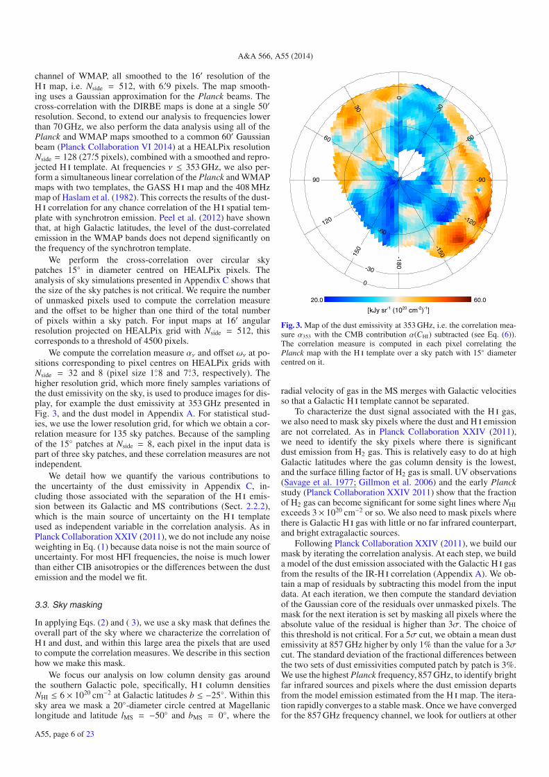
We compute the correlation measure αν and offset ων at po-sitions corresponding to pixel centres on HEALPix grids withNside = 32 and 8 (pixel size 1.◦8 and 7.◦3, respectively). Thehigher resolution grid, which more finely samples variations ofthe dust emissivity on the sky, is used to produce images for dis-play, for example the dust emissivity at 353 GHz presented inFig. 3, and the dust model in Appendix A. For statistical stud-ies, we use the lower resolution grid, for which we obtain a cor-relation measure for 135 sky patches. Because of the samplingof the 15◦ patches at Nside = 8, each pixel in the input data ispart of three sky patches, and these correlation measures are notindependent.

We detail how we quantify the various contributions tothe uncertainty of the dust emissivity in Appendix C, in-cluding those associated with the separation of the H i emis-sion between its Galactic and MS contributions (Sect. 2.2.2),which is the main source of uncertainty on the H i templateused as independent variable in the correlation analysis. As inPlanck Collaboration XXIV (2011), we do not include any noiseweighting in Eq. (1) because data noise is not the main source ofuncertainty. For most HFI frequencies, the noise is much lowerthan either CIB anisotropies or the differences between the dustemission and the model we fit.

3.3. Sky masking

In applying Eqs. (2) and ( 3), we use a sky mask that defines theoverall part of the sky where we characterize the correlation ofH i and dust, and within this large area the pixels that are usedto compute the correlation measures. We describe in this sectionhow we make this mask.

We focus our analysis on low column density gas aroundthe southern Galactic pole, specifically, H i column densitiesNHI ≤ 6 × 1020 cm−2 at Galactic latitudes b ≤ −25◦. Within thissky area we mask a 20◦-diameter circle centred at Magellaniclongitude and latitude lMS = −50◦ and bMS = 0◦, where the

20.0 60.0

[kJy sr-1 (1020 cm-2)-1]

-180

-150

-120

-90

-60

-30

0

30

60

90

120

150

-60

-30

0

Fig. 3. Map of the dust emissivity at 353 GHz, i.e. the correlation mea-sure α353 with the CMB contribution α(CHI) subtracted (see Eq. (6)).The correlation measure is computed in each pixel correlating thePlanck map with the H i template over a sky patch with 15◦ diametercentred on it.

radial velocity of gas in the MS merges with Galactic velocitiesso that a Galactic H i template cannot be separated.

To characterize the dust signal associated with the H i gas,we also need to mask sky pixels where the dust and H i emissionare not correlated. As in Planck Collaboration XXIV (2011),we need to identify the sky pixels where there is significantdust emission from H2 gas. This is relatively easy to do at highGalactic latitudes where the gas column density is the lowest,and the surface filling factor of H2 gas is small. UV observations(Savage et al. 1977; Gillmon et al. 2006) and the early Planckstudy (Planck Collaboration XXIV 2011) show that the fractionof H2 gas can become significant for some sight lines where NHIexceeds 3× 1020 cm−2 or so. We also need to mask pixels wherethere is Galactic H i gas with little or no far infrared counterpart,and bright extragalactic sources.

Following Planck Collaboration XXIV (2011), we build ourmask by iterating the correlation analysis. At each step, we builda model of the dust emission associated with the Galactic H i gasfrom the results of the IR-H i correlation (Appendix A). We ob-tain a map of residuals by subtracting this model from the inputdata. At each iteration, we then compute the standard deviationof the Gaussian core of the residuals over unmasked pixels. Themask for the next iteration is set by masking all pixels where theabsolute value of the residual is higher than 3σ. The choice ofthis threshold is not critical. For a 5σ cut, we obtain a mean dustemissivity at 857 GHz higher by only 1% than the value for a 3σcut. The standard deviation of the fractional differences betweenthe two sets of dust emissivities computed patch by patch is 3%.We use the highest Planck frequency, 857 GHz, to identify brightfar infrared sources and pixels where the dust emission departsfrom the model emission estimated from the H i map. The itera-tion rapidly converges to a stable mask. Once we have convergedfor the 857 GHz frequency channel, we look for outliers at other

A55, page 6 of 23

Planck Collaboration: Dust emission from the diffuse interstellar medium

-0.4 -0.2 0.0 0.2 0.4 0.6Residual emission at 857 GHz [MJy sr-1]

0

5.0•103

1.0•104

1.5•104

2.0•104

2.5•104

3.0•104

Num

ber

of s

ky p

ixel

s

Fig. 4. Histogram of residual emission at 857 GHz after subtractionof the dust emission associated with HI gas. The blue solid line isa Gaussian fit to the core of the histogram, with dispersion σ =0.07 MJy sr−1. We mask pixels where the absolute value of the resid-ual emission is higher than 3σ. The positve (negative) wing of the his-togram beyond this threshold represents 7% (2%) of the data.

frequencies. This is necessary to mask a few infrared galaxies at100 μm and bright radio sources at microwave frequencies. Weperform this procedure with the maps at 16′, 50′, and 60′ reso-lution, obtaining a separate mask for each resolution.

Figure 4 presents the histogram of the residual map at857 GHz with 16′ resolution. The mask discards the positive andnegative tails that depart from the Gaussian fit of the central coreof the histogram. These tails amount to 9% of the total area ofthe residual map.

A sky image of the mask used in the analysis of HFI mapsat 16′ resolution is shown in Fig. 5. The total area not masked is7500 deg2 (18% of the sky). The median NHI is 2.1×1020 H cm−2,and NHI < 3 × 1020 H cm−2 for 74% of the unmasked pixels.

3.4. Galactic residuals with respect to the dust-H I correlation

In this section, we describe the Galactic residuals with respect tothe dust-H i correlation. A power spectrum analysis of the CIBanisotropies over the cleanest part of the southern Galactic capis presented in Planck Collaboration XXX (2014).

Figure 6 shows the map of residual emission at 857 GHz to-gether with the map of H i emission in the MS. The first strikingresult from Fig. 6 is that the residual map shows no evidence ofdust emission from the MS. This result indicates that the MS isdust poor; it will be detailed in a dedicated paper.

The residual map shows localized regions, both positive andnegative, that produce the non-Gaussian wings of the histogramin Fig. 4. The positive residuals are likely to trace dust emis-sion associated with molecular gas (Desert et al. 1988; Reachet al. 1998; Planck Collaboration XXIV 2011). In addition, some

-180

-150

-120

-90

-60

-30

0

30

60

90

120

150

-60

-30

0

Fig. 5. Mask for our analysis of the Planck-H i correlation. The colouredarea that is not blue defines the data used to compute the correlationmeasures. Within this area, the median NHI is 2.1 × 1020 H cm−2, andNHI < 3 × 1020 H cm−2 for 74% of the pixels. The blue patches corre-spond to regions where the absolute value of the residual emission ishigher than 3σ at 857 GHz (Fig. 4). The circular hole near the SouthernGalactic pole corresponds to the area where H i gas in the Galaxy can-not be well separated because the mean radial velocity of the gas in theMS is within the Galactic range of velocities.

positive residuals may be from dust emission associated withGalactic IVC gas not in the Galactic H i template.

The non-Gaussian tail toward negative residuals was not sig-nificant in the earlier higher resolution Planck study that anal-ysed a much smaller sky area at low H i column densities.However, that analysis deduced emissivities for low velocity gasand IVC gas independently, and did find many examples of IVCswith less than half the typical emissivity. If such gas were in-cluded in the Galactic H i template for |vdev| ≤ 45 km s−1, thennegative residuals could arise. Another interesting possible in-terpretation, which needs to be tested, is that negative residualscorrespond to H i gas at Galactic velocities with no or deficientdust emission, akin to the MS, or to typical HVC gas (Peek et al.2009; Planck Collaboration XXIV 2011). We do not discuss fur-ther these regions that are masked in our data analysis. Instead,we focus our analysis on the fainter residuals of Galactic emis-sion that together with CIB anisotropies make the Gaussian coreof the histogram in Fig. 4.

To characterize the Gaussian component of the residualswith respect to the dust-H i correlation, we compute the stan-dard deviation σ857 of the residual map at 857 GHz within cir-cular apertures of 5◦ diameter centred on Nside = 16 pixels. Wechoose this aperture size to be smaller than the sky patches usedto compute the dust emissivity so as to sample more finely σ857.Within each 5◦ aperture, we compute the standard deviation ofthe residual 857 GHz map and the mean NHI over unmasked pix-els, requiring at least 1000 of the maximum 1500 pixels avail-able at Nside = 512. In Fig. 7, σ857 is plotted versus the meanNHI. The hatched strip in the figure indicates the contribution to

A55, page 7 of 23

A&A 566, A55 (2014)

−0.30 0.30

[MJy sr-1]

-180

-150

-120

-90

-60

-30

0

30

60

90

120

150

-60

-30

0

0.0 2.0

[1020 cm-2]

-180

-150

-120

-90

-60

-30

0

30

60

90

120

150

-60

-30

0

Fig. 6. Left: image of the residual emission at 857 GHz obtained by subtracting the H i-based model of the dust emission from the input Planckmap. Right: image of NHI from the Magellanic Stream (see Sect. 2.2.2), the sum of the IVC and HVC maps in Fig. 2.

1 2 3 4NHI [1020 H cm-2]

0.00

0.02

0.04

0.06

0.08

0.10

0.12

0.14

σ 857

[MJy

sr-1

]

CIBAnisotropies

Fig. 7. Standard deviation σ857 of the residuals with respect to thePlanck-H i correlation at 857 GHz versus the mean NHI, both computedwithin circular sky patches with 5◦ diameter and over unmasked pix-els. The red hatched strip marks the contribution of CIB anisotropiesto the residuals at 16′ resolution, computed from the CIB model inPlanck Collaboration XXX (2014). The width of the strip representsthe expected scatter (±1σ) of this contribution. Both the scattered dis-tribution of data points above CIB anisotropies strip and the increasein the mean σ857 with NHI arise from residuals with a Galactic origin(Appendix D).

σ857 from CIB anisotropies at 16′ resolution, as computed usingthe model power spectrum in Planck Collaboration XXX (2014).Most values of σ857 are above the strip. Since the contribution ofnoise to σ857 is negligible, there is a significant contribution toσ857 from residuals with a Galactic origin. The statistical prop-erties of σ857 – the mean trend with increasing NHI and the largescatter around this trend in Fig. 7 – can be accounted for by asimple model where the Galactic residuals arise from variations

of the dust emissivity on scales lower than the 15◦ diameter ofthe patches in our correlation analysis. In Appendix D, we quan-tify this interpretation with simulations.

The ratio of the dispersions from Galactic residuals and fromCIB anisotropies increases towards higher frequencies, but it de-creases with decreasing patch size used in the underlying corre-lation analysis and with better angular resolution of the H i tem-plate map (Appendix C). Thereby an obvious Galactic contri-bution in the faintest fields was not noticed in the earlier studywith the GBT of Planck Collaboration XXIV (2011), but theydid find an increase in the standard deviation of the residualswith the mean column density (see their Fig. 12).

Unlike the localized features that make the non-Gaussianpart of the histogram in Fig. 4, the Gaussian contribution cannotbe masked out. As discussed in Planck Collaboration XXX(2014), it significantly biases the power spectrum ofCIB anisotropies at � < 100, depending on the range ofNHI within the part of the sky used for the analysis.

4. Dust emission properties across the southernGalactic cap

In this section, we use the results from our analysis of the dust-H i correlation to describe how dust emission properties varyacross the southern Galactic cap.

4.1. Dust temperature and opacity

At frequencies higher than 353 GHz, our analysis extends thatof Planck Collaboration XXIV (2011) to a wider area. The dustemissivities are consistent with earlier values, once we correctthem for the change in calibration of the 857 and 545 GHzdata that occurred after the publication of the Planck EarlyPapers (Planck Collaboration VIII 2014). The dust emissivityis observed to vary over the sky in a correlated way between

A55, page 8 of 23

Planck Collaboration: Dust emission from the diffuse interstellar medium

1.5 12.0

10-27 [cm2 H-1]

-180

-150

-120

-90

-60

-30

0

30

60

90

120

150

-60

-30

0

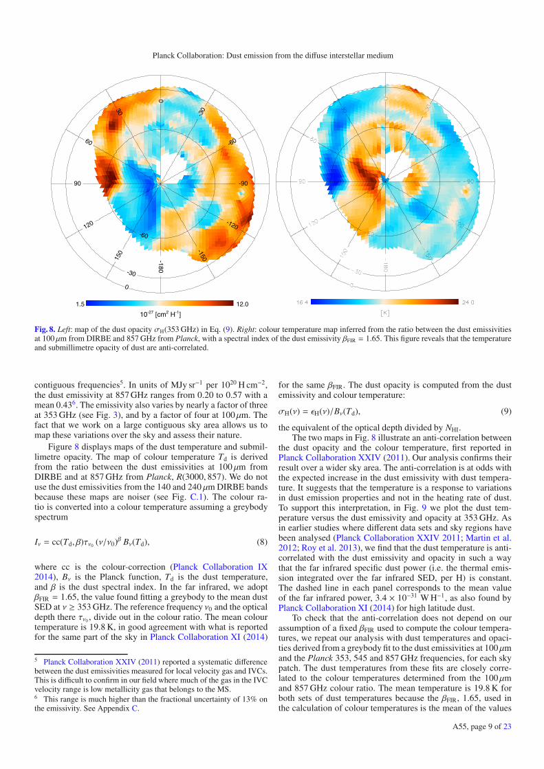
Fig. 8. Left: map of the dust opacity σH(353 GHz) in Eq. (9). Right: colour temperature map inferred from the ratio between the dust emissivitiesat 100 μm from DIRBE and 857 GHz from Planck, with a spectral index of the dust emissivity βFIR = 1.65. This figure reveals that the temperatureand submillimetre opacity of dust are anti-correlated.

contiguous frequencies5. In units of MJy sr−1 per 1020 H cm−2,the dust emissivity at 857 GHz ranges from 0.20 to 0.57 with amean 0.436. The emissivity also varies by nearly a factor of threeat 353 GHz (see Fig. 3), and by a factor of four at 100μm. Thefact that we work on a large contiguous sky area allows us tomap these variations over the sky and assess their nature.

Figure 8 displays maps of the dust temperature and submil-limetre opacity. The map of colour temperature Td is derivedfrom the ratio between the dust emissivities at 100 μm fromDIRBE and at 857 GHz from Planck, R(3000, 857). We do notuse the dust emissivities from the 140 and 240 μm DIRBE bandsbecause these maps are noiser (see Fig. C.1). The colour ra-tio is converted into a colour temperature assuming a greybodyspectrum

Iν = cc(Td, β)τν0 (ν/ν0)β Bν(Td), (8)

where cc is the colour-correction (Planck Collaboration IX2014), Bν is the Planck function, Td is the dust temperature,and β is the dust spectral index. In the far infrared, we adoptβFIR = 1.65, the value found fitting a greybody to the mean dustSED at ν ≥ 353 GHz. The reference frequency ν0 and the opticaldepth there τν0 , divide out in the colour ratio. The mean colourtemperature is 19.8 K, in good agreement with what is reportedfor the same part of the sky in Planck Collaboration XI (2014)

5 Planck Collaboration XXIV (2011) reported a systematic differencebetween the dust emissivities measured for local velocity gas and IVCs.This is difficult to confirm in our field where much of the gas in the IVCvelocity range is low metallicity gas that belongs to the MS.6 This range is much higher than the fractional uncertainty of 13% onthe emissivity. See Appendix C.

for the same βFIR. The dust opacity is computed from the dustemissivity and colour temperature:

σH(ν) = εH(ν)/Bν(Td), (9)

the equivalent of the optical depth divided by NHI.The two maps in Fig. 8 illustrate an anti-correlation between

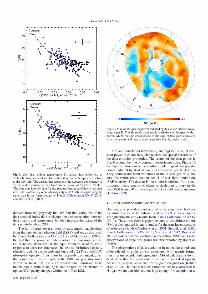
the dust opacity and the colour temperature, first reported inPlanck Collaboration XXIV (2011). Our analysis confirms theirresult over a wider sky area. The anti-correlation is at odds withthe expected increase in the dust emissivity with dust tempera-ture. It suggests that the temperature is a response to variationsin dust emission properties and not in the heating rate of dust.To support this interpretation, in Fig. 9 we plot the dust tem-perature versus the dust emissivity and opacity at 353 GHz. Asin earlier studies where different data sets and sky regions havebeen analysed (Planck Collaboration XXIV 2011; Martin et al.2012; Roy et al. 2013), we find that the dust temperature is anti-correlated with the dust emissivity and opacity in such a waythat the far infrared specific dust power (i.e. the thermal emis-sion integrated over the far infrared SED, per H) is constant.The dashed line in each panel corresponds to the mean valueof the far infrared power, 3.4 × 10−31 W H−1, as also found byPlanck Collaboration XI (2014) for high latitude dust.

To check that the anti-correlation does not depend on ourassumption of a fixed βFIR used to compute the colour tempera-tures, we repeat our analysis with dust temperatures and opaci-ties derived from a greybody fit to the dust emissivities at 100μmand the Planck 353, 545 and 857 GHz frequencies, for each skypatch. The dust temperatures from these fits are closely corre-lated to the colour temperatures determined from the 100μmand 857 GHz colour ratio. The mean temperature is 19.8 K forboth sets of dust temperatures because the βFIR, 1.65, used inthe calculation of colour temperatures is the mean of the values

A55, page 9 of 23

A&A 566, A55 (2014)

0.01 0.02 0.03 0.04 0.05 0.06εH(353GHz) [MJy sr-1 for 1020 H cm-2]

16

18

20

22

24

Td

[K]

ConstantPower

2 4 6 8 10 12σH(353GHz) [10-27 cm2 H-1]

16

18

20

22

24

Td

[K]

ConstantPower

Fig. 9. Top: dust colour temperature Td versus dust emissivity at353 GHz, two independent observables (Fig. 3), with typical error barsat the top right. The dashed line represents the expected dependency ofTd on the dust emissivity for a fixed emitted power of 3.4×10−31 W H−1.The blue dots identify data for sky patches centred at Galactic latitudesb ≤ −60◦. Bottom: Td versus dust opacity at 353 GHz, re-expressing thesame data in the form plotted by Planck Collaboration XXIV (2011)and Martin et al. (2012).

derived from the greybody fits. We find that variations of thedust spectral index do not change the anti-correlation betweendust opacity and temperature, but they increase the scatter of thedata points by about 20%.

The far infrared power emitted by dust equals that absorbedfrom the interstellar radiation field (ISRF) and so, as discussedby Planck Collaboration XXIV (2011) and Martin et al. (2012),the fact that the power is quite constant has two implications.(1) Increases (decreases) in the equilibrium value of Td are aresponse to decreases (increases) in the dust far infrared opacity(the ability of the dust to emit and thus cool). (2) The optical/UVabsorption opacity of dust must be relatively unchanged, giventhat variations in the strength of the ISRF are probably smallwithin the local ISM. Thus, an observational constraint to beunderstood in grain modeling is that the ratio of far infrared tooptical/UV opacity changes within the diffuse ISM.

1.5 4.5

10-31 [W H-1]

-180

-150

-120

-90

-60

-30

0

30

60

90

120

150

-60

-30

0

Fig. 10. Map of the specific power radiated by dust at far infrared wave-lengths per H. This figure displays spatial variations of the specific dustpower, which may be decomposed as the sum of two parts correlatedwith the opacity and temperature maps (see Fig. 8), respectively.

The anti-correlation between Td and σH(353 GHz) at con-stant power does not fully characterize the spatial variations ofthe dust emission properties. The scatter of the data points inFig. 9 around the line of constant power is not noise. Figure 10displays variations over the southern polar cap of the specificpower radiated by dust at far-IR wavelengths per H (Fig. 8).They could result from variations in the dust-to-gas ratio, thedust absorption cross section per H of star light, and/or theISRF intensity. The dust-to-H mass ratio is inferred from spec-troscopic measurements of elements depletions to vary in thelocal ISM from 0.4% in warm gas to 1% in cold neutral medium(Jenkins 2009).

4.2. Dust evolution within the diffuse ISM

Our analysis provides evidence of a varying ratio betweenthe dust opacity at far infrared and visible/UV wavelengths,strengthening the early results from Planck Collaboration XXIV(2011). These two Planck papers extend to the diffuse atomicISM results reported in many studies for the translucent sectionsof molecular clouds (Cambrésy et al. 2001; Stepnik et al. 2003;Planck Collaboration XXV 2011; Martin et al. 2012; Roy et al.2013). Evidence of dust evolution in the diffuse ISM from far-IRobservations of large dust grains was first reported by Bot et al.(2009).

The observations of dust evolution in molecular clouds areoften related to grain growth associated with mantle forma-tion or grain coagulation/aggregation. Model calculations do in-deed show that the variations in the far infrared dust opacityper unit Av may be accounted for by grain coagulation (Köhleret al. 2012). The fact that such variations are now observed inH i gas, where densities are not high enough for coagulation to

A55, page 10 of 23

Planck Collaboration: Dust emission from the diffuse interstellar medium

occur, challenges this interpretation. It would be more satisfac-tory to propose an interpretation that would account for opacityvariations in both the diffuse ISM and molecular clouds. Jones(2012) and Jones et al. (2013) take steps in this direction by in-troducing evolution of carbon dust composition and propertiesinto their dust model. A quantitative modeling of the data hasyet to be done within this new framework, but the results pre-sented by Jones et al. (2013) are encouraging. The variations inthe far infrared opacity and temperature of dust could trace thedegree of processing by UV photons of hydrocarbon dust formedwithin the ISM.

Alternatively, the variations of the far infrared dust opacitycould result from changes in the composition and structure of sil-icate dust. At the temperature of interstellar dust grains in the dif-fuse ISM, low energy transitions, associated with disorder in thestructure of amorphous solids on atomic scales, contribute to thefar infrared dust opacity. This contribution depends on the dusttemperature and on the composition and structure of the grains(Meny et al. 2007). The dust opacity of silicates is observed inlaboratory experiments (Coupeaud et al. 2011) to depend on pa-rameters describing the amorphous structure of the grains, whichmay evolve in interstellar space through, for example, exposureto cosmic rays.

A different perspective is considered in Martin et al. (2012).Dust evolution might not be ongoing now within the diffuse ISM.Instead, the observations might reflect the varying compositionof interstellar dust after evolution both within molecular cloudsand while recyling back to the diffuse ISM, reaching differentend points.

5. The dust spectral index from submillimetreto millimetre wavelengths

Our analysis of the Planck data allows us to measure the spec-tral index of the thermal dust emission from submillimetreto millimetre wavelengths βmm. This complements measure-ments of the spectral index at far infrared wavelengths βFIR inPlanck Collaboration XI (2014) and many earlier studies (e.g.Dupac et al. 2003).

5.1. Measuring the spectral index

For each circular sky patch, we compute the colour ratioR100(353, 217) = α100

353 GHz/α100217 GHz, where α100

ν is the correlationmeasure at frequency ν corrected for the CMB contribution bysubtracting the correlation measure at 100 GHz (Sect. 3.1). Thecolour ratio is converted into a spectral index using a greybodyspectrum (Eq. (8)). We compute R100(353, 217) for a grid of val-ues of βmm and Td. For each sky patch, adopting the colour tem-perature determined above independently from the R(3000, 857)colour ratio, we find the value of βmm that gives a match withthe observed R100(353, 217). We obtain the βmm map presentedin Fig. 11.

The mean value and standard deviation (dispersion) of βmmare 1.51 and 0.13 for Planck maps without subtraction of themodel of zodiacal emission, and 1.51 and 0.16 for maps with themodel subtracted. The standard deviation of the patch by patchdifference between these two βmm values is 0.10, only slightlylower than the dispersion of each. The mean βmm is in goodagreement with the value of 1.53 estimated for the more dif-fuse atomic regions of the Galactic disk by Planck CollaborationInt. XIV (2014), but it is lower than values close to 2 de-rived from the analysis of COBE data at higher frequencies(Boulanger et al. 1996; Finkbeiner et al. 1999). For comparison,

1.0 2.0

-180

-150

-120

-90

-60

-30

0

30

60

90

120

150

-60

-30

0

Fig. 11. Spectral index βmm of the dust emission derived from the ra-tio between correlation measures at 353 and 217 GHz (both correctedfor the CMB contribution by subtracting the correlation measure at100 GHz) and the colour temperature map in Fig. 8.

we computed a value of βFIR for each sky patch by fitting a grey-body to the dust emissivities at the high frequency Planck chan-nels (ν ≥ 353 GHz) and at 100 μm. The difference βFIR−βmm hasa median value of 0.15, and shows no systematic dependence onthe colour temperature Td.

For the derivation of βmm, we have assumed that the dustemission at 100 GHz is well approximated by a greybody ex-trapolation from 353 to 100 GHz. To check that this assumptiondoes not introduce a bias, we repeat the data analysis on Planckmaps in which the CMB anisotropies have been subtracted usingthe CMB map obtained with SMICA (Planck Collaboration XII2014). This allows us to compute the spectral index βmm(SMICA)directly from the ratio between the 353 and 217 GHz correlationmeasures. The mean value of the differences βmm − βmm(SMICA)is negligible, i.e. there is no bias.

5.2. Variations with dust temperature

Many studies, starting with the early work of Dupac et al. (2003),have reported an anti-correlation between βFIR and dust tempera-ture. Laboratory data on amorphous silicates indicate that, at thetemperature of dust grains in the diffuse ISM, it is at millime-tre wavelengths that the variations of the spectral index may bethe largest (Coupeaud et al. 2011). These laboratory results andastronomical data, have been interpreted within a model wherevariations in the dust spectral index stem from the contribution oflow energy transitions, associated with disorder in the structureof amorphous solids on atomic scales, to the dust opacity (Menyet al. 2007; Paradis et al. 2011). Variations of βmm are also pre-dicted to be possible signatures of the evolution of carbon dust(Jones et al. 2013).

Our analysis allows us to look for such variations over a fre-quency range where the determination of the spectral index isto a large extent decoupled from that of the dust temperature.We determine the dust colour temperature Td and the spectral

A55, page 11 of 23

A&A 566, A55 (2014)

16 18 20 22 24Td [K]

1.0

1.5

2.0

β mm

Fig. 12. Spectral index βmm versus Td for the 135 sky patches. The bluedots distinguish patches centred at Galactic latitude b ≤ −60◦. The un-certainties are derived from simulations. The dashed line is a linear re-gression of βmm on Td, slope (−0.043 ± 0.009) K−1.

index βmm from two independent colour ratios, whereas in farinfrared studies the spectral index βFIR and temperature Td aredetermined simultaneously from a spectral fit of the SED (Shettyet al. 2009; Planck Collaboration XI 2014). Althought Td is usedin the conversion of R100(353, 217) into βmm, the uncertaintyof Td has a marginal impact. Furthermore, the photometric un-certainty of far infrared data is higher than that at ν ≤ 353 GHz,where the data calibration is done on the CMB dipole.

We start quantifying the uncertainties of βmm using the nu-merical simulations presented in the companion Planck paper(Planck Collaboration Int. XXI 2014) that extends this work todust polarization. These simulations include H i correlated dustemission with a fixed spectral index 1.5, dust emission uncorre-lated with H i with a spectral index of 2, noise, CIB anisotropies,and free-free emission. We analyse 800 realizations of simulatedmaps at 100, 143, 217, and 353 GHz with the same procedure asused on the Planck data. For each sky patch, we obtain 800 val-ues of βmm. The additional components do not bias the estimateof βmm, but introduce scatter around the mean input value of 1.5.We use the standard deviation of the extracted βmm values as anoise estimate σβ for each sky patch.

The noise on βmm shows a systematic increase towards lowNHI, something that we also observe for the Planck analysis. Wealso measure the standard deviation of βmm over sky patches foreach simulation. We find a value of 0.079 ± 0.01, lower than thedispersion 0.13 measured on the Planck data. If the simulationsprovide a good estimate of the uncertainties, the higher disper-sion for the data shows that βmm has some variance. This can beappreciated in Fig. 12, where the values of βmm with their un-certainties are plotted versus the dust temperature Td. The plotalso displays the result of a linear regression, which has a slopeof (−0.043± 0.009) K−1. Using the set of temperatures obtainedfrom the greybody fits increases the spread of the data pointsin Fig. 12. The slope is changed to (−0.053 ± 0.007) K−1. Thenon-zero slope implies some variation of βmm, and also suggeststhat βmm and Td are anti-correlated. This would extend to themillimetre range a result that has been reported in many studiesfor βFIR versus Td, but the variations here are small and perhapsonly marginally significant. The constancy of βmm is an obser-vational constraint on the nature of the process at the origin ofvariations of the far-IR dust opacity (Sect. 4.2). We note thatPlanck Collaboration Int. XIV (2014) do not find evidence of ananti-correlation in their analysis of Planck observations of thediffuse emission in the Galactic disk.

6. The spectral energy distribution of Galactic dustin the diffuse ISM

At the Planck-LFI and WMAP frequencies, the signal-to-noiseratio on the dust emissivity for a given sky patch is very low be-cause the signal is very faint compared to CMB anisotropies andnoise. However, by averaging the emissivities over sky patches,we obtain an SED of dust emission spanning the full spectralrange and computed consistently at all frequencies (Sect. 6.1).We present greybody fits of the thermal emission of dust atν ≥ 100 GHz in Sect. 6.2. The SED is compared with existingmodels in Sect. 6.3.

6.1. The SED of the mean dust emissivity

We produce a mean SED of dust in the diffuse ISM by averagingthe correlation measures, after correction for the CMB contri-bution as described in Appendix B, over the 135 sky patcheson our lower resolution grid (Sect. 3.2). This SED characterizesthe mean emission properties of dust in atomic gas in the localISM. The statistical uncertainty of the mean SED is computedfrom the standard deviation of individual measurements dividedby the square root of the number of independent sky patches(135/3) used. On average, each pixel of the images is part of3 sky patches. This is why we consider that the number of inde-pendent sky patches is the total number divided by 3. This stan-dard estimate is appropriate for the noisier low frequency data.For the emissivities at higher frequencies, we observe large vari-ations over the sky (Sect. 4.1). However, analysis of our simu-lations (Appendix C) shows that the uncertainties, including thevariations of the emission properties over the sky, average outwhen we compute the mean dust emissivity over sky patches.Mean emissivities with statistical and photometric uncertaintiesare listed in Table 1 for the 16′ resolution maps at ν ≥ 70 GHz.

6.2. Greybody fits

We characterize the dust SED with greybody fits. The meanemissivities are weighted using uncertainties that are thequadratic combination of the statistical and photometric uncer-tainties. We map the χ2 for greybody spectra over the parameterspace to determine the best fit parameters listed in Table 3. Wereport parameters from data without and with subtraction of thezodiacal emission model (Planck Collaboration XIV 2014). Thedifferences in fit parameters are within the uncertainties. This isto be expected because the zodiacal emission is a slowly varyingfunction uncorrelated with the spatial fluctuations of the H i tem-plate within the 15◦ patches.

All of the best fits have χ2 per degree of freedom muchlower than 1, because the statistical and photometric uncertain-ties are correlated across frequencies. To test our fits and to esti-mate error bars on the parameters, we run a Monte-Carlo sim-ulation that takes these correlations into account. We assumethat the photometric uncertainties are correlated for the threeDIRBE frequencies, for the two highest HFI frequencies cali-brated on planets, and for the four lowest HFI frequencies cal-ibrated on the CMB dipole. For the statistical errors, we usethe frequency-dependent decomposition into Galactic, CMB,CIB, and noise contributions inferred from the sky simulationsin Appendix C. The sky simulations ignore the decorrelationfrom far infrared to microwave frequencies of CIB anisotropies(Planck Collaboration XXX 2014) and of Galactic residuals dueto variations in dust temperature. These two shortcomings arenot an issue, because they mainly impact the modeling of the

A55, page 12 of 23

Planck Collaboration: Dust emission from the diffuse interstellar medium

Table 1. Mean SED of dust emissivity from H i correlation.

Frequency [GHz]Experiment

70 94 100 143 217 353 545 857 1249 2143 2997Quantity LFI WMAP HFI HFI HFI HFI HFI HFI DIRBE DIRBE DIRBE

εH(ν) [MJy sr−1 (1020 H cm−2)−1] . . . 0.00027 0.00045 0.00067 0.0020 0.0086 0.039 0.14 0.43 0.84 1.1 0.63σstat [MJy sr−1 (1020 H cm−2)−1] . . . . 2.8 × 10−5 8.9 × 10−5 2.8 × 10−5 7.9 × 10−5 3.0 × 10−4 0.0013 0.0045 0.013 0.027 0.048 0.022photunc [%] . . . . . . . . . . . . . . . . . 0.5 0.2 0.5 0.5 0.5 1.2 10.0 10.0 11.6 10.6 13.6σtot [MJy sr−1 (1020 H cm−2)−1] . . . . 2.8 × 10−5 8.9 × 10−5 2.8 × 10−5 7.9 × 10−5 3.0 × 10−4 0.0014 0.015 0.045 0.10 0.13 0.088cc . . . . . . . . . . . . . . . . . . . . . . . 0.96 0.98 1.09 1.02 1.12 1.11 1.10 1.02 1.00 0.94 0.92uc . . . . . . . . . . . . . . . . . . . . . . . 7.54 4.63 4.10 2.69 2.07 3.48 . . . . . . . . . . . . . . .

Notes. εH(ν) ≡ Mean dust emissivity εH(ν) expressed as monochromatic brightness at the reference frequencies, derived from correlation of themaps with the Galactic H i template. Not colour corrected. σstat ≡ Statistical uncertainty (1σ) of the mean emissivities. photunc (%) ≡ Uncertaintiesof the absolute calibration [%] from Planck Collaboration I (2014), Bennett et al. (2013), and Hauser et al. (1998). σtot ≡ Total uncertaintycombining statistical and photometric uncertainties [MJy sr−1 per 1020 H cm−2]. cc ≡ Colour-correction factors in Eq. (8) computed with thegreybody parameters listed in Table 3. uc ≡ Unit conversion factors from MJy sr−1 to thermodynamic (CMB) temperatures in mK.

Table 2. Mean microwave SED from H i correlation.

Frequency [GHz]Experiment

23 28.4 33 41 44.1 61 70.4 94 100 143 217 353Quantity WMAP LFI WMAP WMAP LFI WMAP LFI WMAP HFI HFI HFI HFI

εH(ν) [μKRJ (1020 H cm−2)−1] . . . . . . . . . . . . . . . . . . 17. 9.6 6.7 3.7 3.0 2.0 1.7 1.8 2.1 3.2 6.0 10.4σstat [μKRJ (1020 H cm−2)−1] . . . . . . . . . . . . . . . . . . . 1.4 0.92 0.60 0.38 0.31 0.23 0.17 0.26 0.087 0.12 0.19 0.31ε′H(ν) [μKRJ (1020 H cm−2)−1] . . . . . . . . . . . . . . . . . . 14. 7.8 5.4 3.1 2.5 1.9 1.6 1.6 2.2 3.2 6.0 10.3σ′stat [μKRJ (1020 H cm−2)−1] . . . . . . . . . . . . . . . . . . . 1.2 0.72 0.64 0.42 0.34 0.27 0.20 0.27 0.11 0.12 0.19 0.31ucK . . . . . . . . . . . . . . . . . . . . . . . . . . . . . . . . . . . 1.01 0.92 1.03 1.04 1.06 1.10 1.15 1.26 1.26 1.69 2.99 13.3

Notes. εH and ε′H ≡ Mean dust emissivity expressed as monochromatic brightness at the reference frequencies from the correlation of the mapswith the Galactic H i template alone, and with both the Galactic H i template and the 408 MHz map, respectively. Not colour corrected. σstat andσ′stat ≡ Statistical uncertainty (1σ) of the brightness temperatures Tb and T ′b. ucK ≡ Unit conversion factors from brightness (Rayleigh-Jeans)to thermodynamic (CMB) temperature. For WMAP the conversion factors are computed at the reference frequency, while for Planck they arecomputed assuming a constant ν Iν within the spectral band.

Table 3. Parameters from greybody fits of the mean dust SED.

Model parameters

σH(353 GHz) Td βFIR βmm χ2/d.o.f.Model [cm2 H−1] [K]

Without subtraction of zodiacal emission . . .ν ≥ 353 GHz . . . . . . . . . . . . . . . . . . . . . . (7.3 ± 0.65) × 10−27 19.8 ± 1.0 1.65 ± 0.10 . . . 0.05ν ≥ 100 GHz . . . . . . . . . . . . . . . . . . . . . . (6.9 ± 0.5 ) × 10−27 21.0 ± 0.7 1.52 ± 0.03 . . . 0.22ν ≥ 100 GHz with 2 β . . . . . . . . . . . . . . . . (7.3 ± 0.6 ) × 10−27 19.8 ± 1.0 1.65 ± 0.10 1.52 ± 0.03 0.041

With subtraction of zodiacal emission . . . .ν ≥ 353 GHz . . . . . . . . . . . . . . . . . . . . . . (7.1 ± 0.65) × 10−27 19.9 ± 1.0 1.65 ± 0.10 . . . 0.07ν ≥ 100 GHz . . . . . . . . . . . . . . . . . . . . . . (6.8 ± 0.5 ) × 10−27 21.0 ± 0.7 1.53 ± 0.03 . . . 0.19ν ≥ 100 GHz with 2 β . . . . . . . . . . . . . . . . (7.2 ± 0.6 ) × 10−27 19.9 ± 1.0 1.65 ± 0.10 1.54 ± 0.03 0.060

Notes. σH(353 GHz) ≡ Dust opacity at 353 GHz from greybody fit. Td ≡ Dust temperature from greybody fit. βFIR ≡ Spectral index for ν ≥353 GHz for models 1 and 3, and for ν ≥ 100 GHz for model 2. βmm ≡ Spectral index for ν ≤ 353 GHz for model 3. χ2/d.o.f. ≡ χ2 of the fit perdegree of freedom.

statistical uncertainties at far infrared frequencies where the pho-tometric uncertainties are dominant. We apply our fits to a grey-body spectrum with βFIR = βmm = 1.55 and Td = 19.8 K, com-bined with 1000 realizations of the statistical and photometricuncertainties. For each realization, we obtain a set of values forthe parameters of the fit. For each of the three fits in Table 3,we compute the average and standard deviation of the param-eters. The average values match the input values, showing thatcorrelated uncertainties do not bias the fit. We list the standarddeviations from the Monte Carlo simulation as error bars for the

fit parameters in Table 3. We are confident about this estimate ofthe errors because the χ2 values obtained for the data fits are inthe core of the χ2 distribution for the Monte Carlo simulation. Inother words, the simulation accounts for the low values of the χ2

per degree of freedom in Table 3.The first fit is for frequencies ν ≥ 353 GHz. It is di-

rectly comparable to the fits presented in the all-sky analysisof Planck Collaboration XI (2014). The spectral index that wefind, β = 1.65± 0.10, agrees with the mean value used in Sect. 4to compute colour temperatures, but it is greater than the values

A55, page 13 of 23

A&A 566, A55 (2014)

of βmm = 1.51 ± 0.13 derived from the R100(353, 217) ratio inSect. 5. The second fit extends the greybody fit with a singlespectral index down to 100 GHz. This fit yields a spectral in-dex of 1.52 ± 0.03 in agreement with the mean value inferredfrom the above R100(353, 217) ratio. For the latter, the dispersionabout the mean is higher than the uncertainty from the fit, whichis more like an uncertainty of the mean.

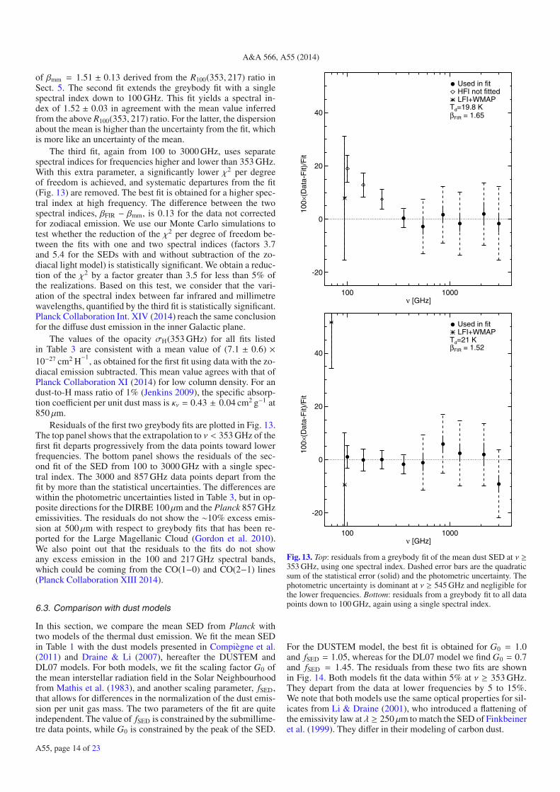
The third fit, again from 100 to 3000 GHz, uses separatespectral indices for frequencies higher and lower than 353 GHz.With this extra parameter, a significantly lower χ2 per degreeof freedom is achieved, and systematic departures from the fit(Fig. 13) are removed. The best fit is obtained for a higher spec-tral index at high frequency. The difference between the twospectral indices, βFIR − βmm, is 0.13 for the data not correctedfor zodiacal emission. We use our Monte Carlo simulations totest whether the reduction of the χ2 per degree of freedom be-tween the fits with one and two spectral indices (factors 3.7and 5.4 for the SEDs with and without subtraction of the zo-diacal light model) is statistically significant. We obtain a reduc-tion of the χ2 by a factor greater than 3.5 for less than 5% ofthe realizations. Based on this test, we consider that the vari-ation of the spectral index between far infrared and millimetrewavelengths, quantified by the third fit is statistically significant.Planck Collaboration Int. XIV (2014) reach the same conclusionfor the diffuse dust emission in the inner Galactic plane.

The values of the opacity σH(353 GHz) for all fits listedin Table 3 are consistent with a mean value of (7.1 ± 0.6) ×10−27 cm2 H−1, as obtained for the first fit using data with the zo-diacal emission subtracted. This mean value agrees with that ofPlanck Collaboration XI (2014) for low column density. For andust-to-H mass ratio of 1% (Jenkins 2009), the specific absorp-tion coefficient per unit dust mass is κν = 0.43 ± 0.04 cm2 g−1 at850 μm.

Residuals of the first two greybody fits are plotted in Fig. 13.The top panel shows that the extrapolation to ν < 353 GHz of thefirst fit departs progressively from the data points toward lowerfrequencies. The bottom panel shows the residuals of the sec-ond fit of the SED from 100 to 3000 GHz with a single spec-tral index. The 3000 and 857 GHz data points depart from thefit by more than the statistical uncertainties. The differences arewithin the photometric uncertainties listed in Table 3, but in op-posite directions for the DIRBE 100μm and the Planck 857 GHzemissivities. The residuals do not show the ∼10% excess emis-sion at 500 μm with respect to greybody fits that has been re-ported for the Large Magellanic Cloud (Gordon et al. 2010).We also point out that the residuals to the fits do not showany excess emission in the 100 and 217 GHz spectral bands,which could be coming from the CO(1−0) and CO(2−1) lines(Planck Collaboration XIII 2014).

6.3. Comparison with dust models

In this section, we compare the mean SED from Planck withtwo models of the thermal dust emission. We fit the mean SEDin Table 1 with the dust models presented in Compiègne et al.(2011) and Draine & Li (2007), hereafter the DUSTEM andDL07 models. For both models, we fit the scaling factor G0 ofthe mean interstellar radiation field in the Solar Neighbourhoodfrom Mathis et al. (1983), and another scaling parameter, fSED,that allows for differences in the normalization of the dust emis-sion per unit gas mass. The two parameters of the fit are quiteindependent. The value of fSED is constrained by the submillime-tre data points, while G0 is constrained by the peak of the SED.

100 1000ν [GHz]

-20

0

20

40

100×

(Dat

a-F

it)/F

it

Used in fitHFI not fittedLFI+WMAP

Td=19.8 KβFIR = 1.65

100 1000ν [GHz]

-20

0

20

40

100×

(Dat

a-F

it)/F

it

Used in fitLFI+WMAP

Td=21 KβFIR = 1.52

Fig. 13. Top: residuals from a greybody fit of the mean dust SED at ν ≥353 GHz, using one spectral index. Dashed error bars are the quadraticsum of the statistical error (solid) and the photometric uncertainty. Thephotometric uncertainty is dominant at ν ≥ 545 GHz and negligible forthe lower frequencies. Bottom: residuals from a greybody fit to all datapoints down to 100 GHz, again using a single spectral index.

For the DUSTEM model, the best fit is obtained for G0 = 1.0and fSED = 1.05, whereas for the DL07 model we find G0 = 0.7and fSED = 1.45. The residuals from these two fits are shownin Fig. 14. Both models fit the data within 5% at ν ≥ 353 GHz.They depart from the data at lower frequencies by 5 to 15%.We note that both models use the same optical properties for sil-icates from Li & Draine (2001), who introduced a flattening ofthe emissivity law at λ ≥ 250 μm to match the SED of Finkbeineret al. (1999). They differ in their modeling of carbon dust.

A55, page 14 of 23

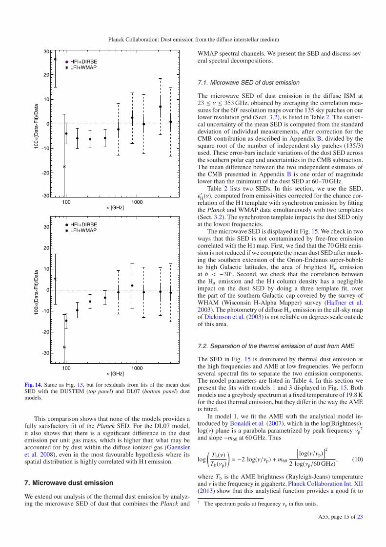
Planck Collaboration: Dust emission from the diffuse interstellar medium

100 1000ν [GHz]

-30

-20

-10

0

10

20

30

100×

(Dat

a-F

it)/D

ata

HFI+DIRBELFI+WMAP

100 1000ν [GHz]

-30

-20

-10

0

10

20

30

100×

(Dat

a-F

it)/D

ata

HFI+DIRBELFI+WMAP

Fig. 14. Same as Fig. 13, but for residuals from fits of the mean dustSED with the DUSTEM (top panel) and DL07 (bottom panel) dustmodels.

This comparison shows that none of the models provides afully satisfactory fit of the Planck SED. For the DL07 model,it also shows that there is a significant difference in the dustemission per unit gas mass, which is higher than what may beaccounted for by dust within the diffuse ionized gas (Gaensleret al. 2008), even in the most favourable hypothesis where itsspatial distribution is highly correlated with H i emission.

7. Microwave dust emission

We extend our analysis of the thermal dust emission by analyz-ing the microwave SED of dust that combines the Planck and

WMAP spectral channels. We present the SED and discuss sev-eral spectral decompositions.

7.1. Microwave SED of dust emission

The microwave SED of dust emission in the diffuse ISM at23 ≤ ν ≤ 353 GHz, obtained by averaging the correlation mea-sures for the 60′ resolution maps over the 135 sky patches on ourlower resolution grid (Sect. 3.2), is listed in Table 2. The statisti-cal uncertainty of the mean SED is computed from the standarddeviation of individual measurements, after correction for theCMB contribution as described in Appendix B, divided by thesquare root of the number of independent sky patches (135/3)used. These error-bars include variations of the dust SED acrossthe southern polar cap and uncertainties in the CMB subtraction.The mean difference between the two independent estimates ofthe CMB presented in Appendix B is one order of magnitudelower than the minimum of the dust SED at 60–70 GHz.

Table 2 lists two SEDs. In this section, we use the SED,ε′H(ν), computed from emissivities corrected for the chance cor-relation of the H i template with synchrotron emission by fittingthe Planck and WMAP data simultaneously with two templates(Sect. 3.2). The synchrotron template impacts the dust SED onlyat the lowest frequencies.

The microwave SED is displayed in Fig. 15. We check in twoways that this SED is not contaminated by free-free emissioncorrelated with the H i map. First, we find that the 70 GHz emis-sion is not reduced if we compute the mean dust SED after mask-ing the southern extension of the Orion-Eridanus super-bubbleto high Galactic latitudes, the area of brightest Hα emissionat b < −30◦. Second, we check that the correlation betweenthe Hα emission and the H i column density has a negligibleimpact on the dust SED by doing a three template fit, overthe part of the southern Galactic cap covered by the survey ofWHAM (Wisconsin H-Alpha Mapper) survey (Haffner et al.2003). The photometry of diffuse Hα emission in the all-sky mapof Dickinson et al. (2003) is not reliable on degrees scale outsideof this area.

7.2. Separation of the thermal emission of dust from AME

The SED in Fig. 15 is dominated by thermal dust emission atthe high frequencies and AME at low frequencies. We performseveral spectral fits to separate the two emission components.The model parameters are listed in Table 4. In this section wepresent the fits with models 1 and 3 displayed in Fig. 15. Bothmodels use a greybody spectrum at a fixed temperature of 19.8 Kfor the dust thermal emission, but they differ in the way the AMEis fitted.

In model 1, we fit the AME with the analytical model in-troduced by Bonaldi et al. (2007), which in the log(Brightness)-log(ν) plane is a parabola parametrized by peak frequency νp7

and slope −m60 at 60 GHz. Thus

log

(Tb(ν)Tb(νp)

)= −2 log(ν/νp) + m60

[log(ν/νp)

]2

2 log(νp/60 GHz), (10)

where Tb is the AME brightness (Rayleigh-Jeans) temperatureand ν is the frequency in gigahertz. Planck Collaboration Int. XII(2013) show that this analytical function provides a good fit to

7 The spectrum peaks at frequency νp in flux units.

A55, page 15 of 23

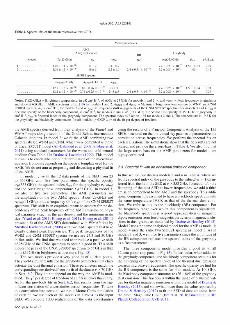
A&A 566, A55 (2014)

Table 4. Spectral fits of the mean microwave dust SED.

Model parameters

AMEAnalytical model Greybody

BBModel Tb(23 GHz) νp −m60 τBB σH(353 GHz) βmm χ2/d.o.f.

1 . . . . . . . . . . . . . . 13.0 ± 1.1 × 10−20 11 ± 7 1.4 ± 0.7 . . . 7.4 ± 0.23 × 10−27 1.52 ± 0.03 0.272 . . . . . . . . . . . . . . 12.6 ± 1.2 × 10−20 19 ± 6 2.2 ± 1.0 2.4 ± 0.51 × 10−28 7.3 ± 0.24 × 10−27 1.65 0.42

SPDUST spectra

AWNM(23 GHz) ACNM(41 GHz) νshift

3 . . . . . . . . . . . . . . 12.8 ± 1.3 × 10−20 0.88 ± 0.26 × 10−20 25 ± 3 . . . 7.4 ± 0.26 × 10−27 1.50 ± 0.04 0.214 . . . . . . . . . . . . . . 12.2 ± 1.2 × 10−20 0.71 ± 0.25 × 10−20 24.5 ± 3 2.4 ± 0.54 × 10−28 7.3 ± 0.26 × 10−27 1.65 0.34

Notes. Tb(23 GHz) ≡ Brightness temperature, in μK cm2 H−1, of AME at 23 GHz for models 1 and 2. νp and −m60 ≡ Peak frequency in gigahertzand slope at 60 GHz of AME spectrum in Eq. (10) for models 1 and 2. AWNM and ACNM ≡Maximum brightness temperature of WNM and CNMSPDUST spectra, in μK cm2 H−1, for models 3 and 4. νshift ≡ Frequency shift in gigahertz of the CNM SPDUST spectrum for models 3 and 4. τBB ≡Specific opacity of the blackbody component, in cm2 H−1, for models 2 and 4. σH(353 GHz) ≡ Specific dust opacity at 353 GHz of greybody incm2 H−1. βmm ≡ Spectral index of the greybody component. The spectral index is fixed to 1.65 for models 2 and 4. The temperature is 19.8 K forthe greybody and blackbody components for all models. χ2/DOF ≡ χ2 of the fit per degree of freedom.

the AME spectra derived from their analysis of the Planck andWMAP maps along a section of the Gould Belt at intermediateGalactic latitudes. In model 3, we fit the AME combining twospectra labeled WNM and CNM, which were computed with thephysical SPDUST model (Ali-Haïmoud et al. 2009; Silsbee et al.2011) using standard parameters for the warm and cold neutralmedium from Table 1 in Draine & Lazarian (1999). This modelallows us to check whether our determination of the microwaveemission from dust depends on the spectral template used for theAME. We do not aim at proposing and discussing a physical fitof the AME.

In model 1, we fit the 12 data points of the SED from 23to 353 GHz with five free parameters: the specific opacityσH(353 GHz); the spectral index βmm for the greybody; νp; m60;and the AME brightness temperature Tb(23 GHz). In model 3,we also fit five free parameters. The AME parameters arethe amplitudes of the two AME spectra, AWNM(23 GHz) andACNM(41 GHz), plus a frequency shift νshift of the CNM SPDUSTspectrum. This shift is an empirical means to account for the de-pendency of the peak frequency of the AME emission on phys-ical parameters such as the gas density and the minimum grainsize (Ysard et al. 2011; Hoang et al. 2011). Hoang et al. (2011)present a fit of the AME SED determined with WMAP data byMiville-Deschênes et al. (2008) with two AME spectra that haveclearly distinct peak frequencies. The peak frequencies of theWNM and CNM SPDUST spectra we use are 24.3 and 30 GHzin flux units. We find that we need to introduce a positive shiftof 25 GHz of the CNM spectrum to obtain a good fit. This shiftmoves the peak of the CNM SPDUST spectrum to 55 GHz in fluxunits (51 GHz in brightness temperature, Fig. 15).

The two models provide a very good fit of all data points.They yield similar results for the greybody parameters that char-acterize the dust thermal emission. These parameters match thecorresponding ones derived from the fit of the data at ν ≥ 70 GHzin Sect. 6.2. They do not depend on the way the AME is mod-elled. The χ2 per degree of freedom of all fits is lower than unity.As for the greybody fits in Sect. 6.2, this results from the sig-nificant correlation of uncertainties across frequencies. To takethis correlation into account, we run a Monte-Carlo simulationof each fit. We use each of the models in Table 4 as the inputSED. We compute 1000 realizations of the data uncertainties

using the results of a Principal Component Analysis of the 135SEDs measured on the individual sky patches to parametrize thecorrelation across frequencies. We perform the spectral fits oneach realization. The simulations show that the fit results are notbiased, and provide the errors-bars in Table 4. We also find thatthe large errors-bars on the AME parameters for model 1 arehighly correlated.

7.3. Spectral fit with an additional emission component

In this section, we discuss models 2 and 4 in Table 4, where wefix the spectral index of the greybody to the value βFIR = 1.65 in-ferred from the fit of the SED at ν ≥ 353 GHz. To account for theflattening of the dust SED at lower frequencies, we add a thirdemission component to the AME and the greybody. This addi-tional component is assumed to have a blackbody spectrum withthe same temperature 19.8 K as that of the thermal dust emis-sion. We refer to this as the blackbody (BB) component. Forthe frequency range over which this component is significant,the blackbody spectrum is a good approximation of magneticdipole emission from ferro-magnetic particles or magnetic inclu-sions in dust grains, as modelled by Draine & Hensley (2013).Model 2 uses the same analytical model for the AME as model 1;model 4 uses the same two SPDUST spectra as model 3. As inmodels 1 and 3, we fit for five parameters since the amplitude ofthe BB component replaces the spectral index of the greybodyas a free parameter.

The three components model provides a good fit to all12 data points (top panel in Fig.15). In particular, when added tothe greybody component, the blackbody component accounts forthe flattening of the spectral index of the thermal dust emissiontowards microwave frequencies. The specific opacity we find forthe BB component is the same for both models. At 100 GHz,the blackbody component amounts to (26±6)% of the greybodydust emission. This fraction is within the range of plausible val-ues for dipolar magnetic emission within the model of Draine &Hensley (2013), and somewhat lower than the value reported byDraine & Hensley (2012) to fit the SED of dust emission fromthe Small Magellanic Cloud (Bot et al. 2010; Israel et al. 2010;Planck Collaboration XVII 2011).

A55, page 16 of 23

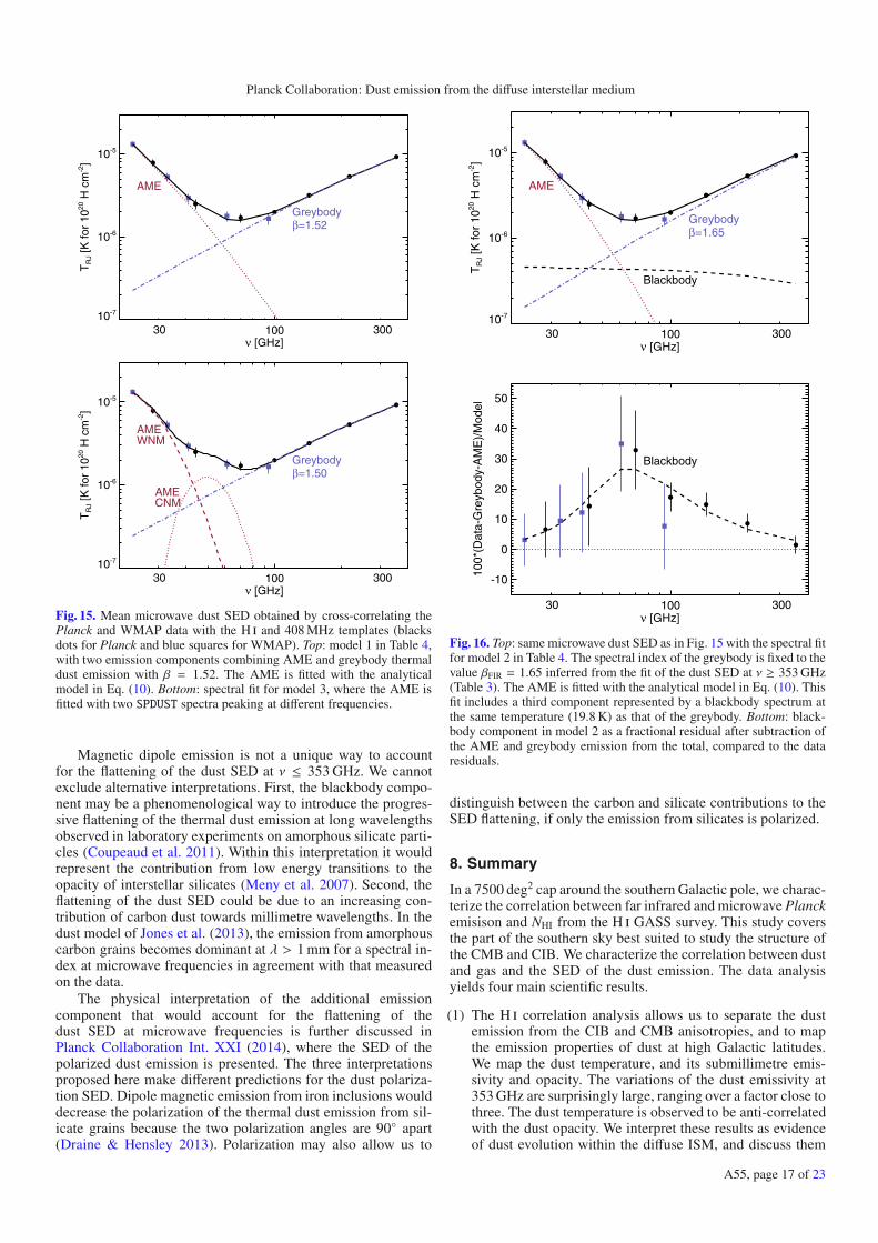
Planck Collaboration: Dust emission from the diffuse interstellar medium

100ν [GHz]

10-7

10-6

10-5

TR

J [K

for

1020

H c

m-2]

30 300

AME

Greybodyβ=1.52

100ν [GHz]

10-7

10-6

10-5

TR

J [K

for

1020

H c

m-2]

30 300

AMEWNM

AMECNM

Greybodyβ=1.50

Fig. 15. Mean microwave dust SED obtained by cross-correlating thePlanck and WMAP data with the H i and 408 MHz templates (blacksdots for Planck and blue squares for WMAP). Top: model 1 in Table 4,with two emission components combining AME and greybody thermaldust emission with β = 1.52. The AME is fitted with the analyticalmodel in Eq. (10). Bottom: spectral fit for model 3, where the AME isfitted with two SPDUST spectra peaking at different frequencies.

Magnetic dipole emission is not a unique way to accountfor the flattening of the dust SED at ν ≤ 353 GHz. We cannotexclude alternative interpretations. First, the blackbody compo-nent may be a phenomenological way to introduce the progres-sive flattening of the thermal dust emission at long wavelengthsobserved in laboratory experiments on amorphous silicate parti-cles (Coupeaud et al. 2011). Within this interpretation it wouldrepresent the contribution from low energy transitions to theopacity of interstellar silicates (Meny et al. 2007). Second, theflattening of the dust SED could be due to an increasing con-tribution of carbon dust towards millimetre wavelengths. In thedust model of Jones et al. (2013), the emission from amorphouscarbon grains becomes dominant at λ > 1 mm for a spectral in-dex at microwave frequencies in agreement with that measuredon the data.

The physical interpretation of the additional emissioncomponent that would account for the flattening of thedust SED at microwave frequencies is further discussed inPlanck Collaboration Int. XXI (2014), where the SED of thepolarized dust emission is presented. The three interpretationsproposed here make different predictions for the dust polariza-tion SED. Dipole magnetic emission from iron inclusions woulddecrease the polarization of the thermal dust emission from sil-icate grains because the two polarization angles are 90◦ apart(Draine & Hensley 2013). Polarization may also allow us to

100ν [GHz]

10-7

10-6

10-5

TR

J [K

for

1020

H c

m-2]

30 300

AME

Blackbody

Greybodyβ=1.65

100ν [GHz]

-10

0

10

20

30

40

50

100*

(Dat

a-G

reyb

ody-

AM

E)/

Mod

el

30 300

Blackbody

Fig. 16. Top: same microwave dust SED as in Fig. 15 with the spectral fitfor model 2 in Table 4. The spectral index of the greybody is fixed to thevalue βFIR = 1.65 inferred from the fit of the dust SED at ν ≥ 353 GHz(Table 3). The AME is fitted with the analytical model in Eq. (10). Thisfit includes a third component represented by a blackbody spectrum atthe same temperature (19.8 K) as that of the greybody. Bottom: black-body component in model 2 as a fractional residual after subtraction ofthe AME and greybody emission from the total, compared to the dataresiduals.

distinguish between the carbon and silicate contributions to theSED flattening, if only the emission from silicates is polarized.

8. Summary

In a 7500 deg2 cap around the southern Galactic pole, we charac-terize the correlation between far infrared and microwave Planckemisison and NHI from the H i GASS survey. This study coversthe part of the southern sky best suited to study the structure ofthe CMB and CIB. We characterize the correlation between dustand gas and the SED of the dust emission. The data analysisyields four main scientific results.

(1) The H i correlation analysis allows us to separate the dustemission from the CIB and CMB anisotropies, and to mapthe emission properties of dust at high Galactic latitudes.We map the dust temperature, and its submillimetre emis-sivity and opacity. The variations of the dust emissivity at353 GHz are surprisingly large, ranging over a factor close tothree. The dust temperature is observed to be anti-correlatedwith the dust opacity. We interpret these results as evidenceof dust evolution within the diffuse ISM, and discuss them

A55, page 17 of 23

A&A 566, A55 (2014)

within the context of existing models of dust. The meandust opacity is measured to be (7.1± 0.6)× 10−27 cm2 H

−1 ×(ν/353 GHz)1.53±0.03, for 100 ≤ ν ≤ 353 GHz. This is a refer-ence value to estimate hydrogen masses from dust emissionat submillimetre and millimetre wavelengths.

(2) Using a colour ratio between 353 and 217 GHz that is freefrom CMB, we determine the spectral index βmm of the dustemission. We find a mean value of 1.51 that is remarkablyconstant over the field of our investigation; the standard de-viation is 0.13. Variations of βmm show no clear trend withthe 353 GHz dust emissivity, nor with the dust temperature.We compare βmm with the spectral index βFIR derived fromgreybody fits at ν ≥ 353 GHz. We find a systematic differ-ence of βmm − βFIR = 0.15.

(3) We fit the SED of the microwave emission correlated withH i from 23 to 353 GHz with two components, a parametricmodel or SPDUST spectra for AME, and a greybody for thethermal dust emission. We show that the flattening of the dustSED at ν ≤ 353 GHz can be accounted for with an additionalblackbody component. This additional component, whichaccounts for (26 ± 6)% of the dust emission at 100 GHz,could represent magnetic dipole emission. Alternatively, itcould represent the contribution from low energy transitionsin amorphous solids to the opacity of interstellar silicates, oran increasing contribution from carbon dust. These interpre-tations make different predictions for the dust polarizationSED measured by Planck.

(4) We analyse the residuals with respect to the dust-H i corre-lation. We identify a Galactic contribution to these residuals,which we model with variations of the dust emissivity onangular scales smaller than the 15◦ patches of our correla-tion analysis. This model of the residuals is used to quan-tify uncertainties of the CIB power spectrum in a companionPlanck paper (Planck Collaboration XXX 2014).

These results are important for defining future models ofdust emission. Such models will need to include the evo-lution/variation of dust properties within the diffuse ISM.They are also valuable inputs to CIB and CMB studies. InPlanck Collaboration XXX (2014), our analysis is used to deter-mine the power spectrum of CIB anisotropies over a field morethan an order of magnitude higher than in earlier studies. Thespectral characterization of the dust emission is being combinedwith the all-sky analysis in Planck Collaboration XI (2014) toprepare a model of dust emission at microwave frequencies forCMB studies.

This paper opens the way to additional studies of the dust-H icorrelation. The methodology introduced in this paper is of gen-eral use to studies of the dust-H i correlation with diverse scienceobjectives. We have focused our scientific analysis on the emis-sion properties of Galactic dust, leaving for further studies sev-eral aspects of the dust-gas correlation. In a future paper we willuse the same data and method to quantify an upper limit on thedust-to-gas mass ratio in the MS gas, and to characterize H i gasat Galactic velocities with no or only a faint counterpart in thePlanck maps. The clouds of excess dust emission with respect tothe H imodel also deserve further attention, to investigate whereH2 forms within the diffuse ISM.

Acknowledgements. The development of Planck has been supported by:ESA; CNES and CNRS/INSU-IN2P3-INP (France); ASI, CNR, and INAF(Italy); NASA and DoE (USA); STFC and UKSA (UK); CSIC, MICINN,JA and RES (Spain); Tekes, AoF and CSC (Finland); DLR and MPG(Germany); CSA (Canada); DTU Space (Denmark); SER/SSO (Switzerland);RCN (Norway); SFI (Ireland); FCT/MCTES (Portugal); and PRACE (EU).

A description of the Planck Collaboration and a list of its members, includ-ing the technical or scientific activities in which they have been involved, canbe found at http://www.sciops.esa.int/index.php?project=planck&page=Planck_Collaboration. The Parkes Radio Telescope is part of theAustralia Telescope, which is funded by the Commonwealth of Australia foroperation as a National Facility managed by CSIRO. The research leading tothese results has received funding from the European Research Council underthe European Union’s Seventh Framework Programme (FP7/2007-2013)/ERCgrant agreement n◦ 267934.

ReferencesAli-Haïmoud, Y., Hirata, C. M., & Dickinson, C. 2009, MNRAS, 395, 1055Arendt, R. G., Odegard, N., Weiland, J. L., et al. 1998, ApJ, 508, 74Banday, A. J., Dickinson, C., Davies, R. D., Davis, R. J., & Górski, K. M. 2003,

MNRAS, 345, 897Bennett, C. L., Larson, D., Weiland, J. L., et al. 2013, ApJS, 208, 20Bersanelli, M., Mandolesi, N., Butler, R. C., et al. 2010, A&A, 520, A4Bonaldi, A., Ricciardi, S., Leach, S., et al. 2007, MNRAS, 382, 1791Bot, C., Helou, G., Boulanger, F., et al. 2009, ApJ, 695, 469Bot, C., Ysard, N., Paradis, D., et al. 2010, A&A, 523, A20Boulanger, F., & Perault, M. 1988, ApJ, 330, 964Boulanger, F., Abergel, A., Bernard, J.-P., et al. 1996, A&A, 312, 256Cambrésy, L., Boulanger, F., Lagache, G., & Stepnik, B. 2001, A&A, 375, 999Compiègne, M., Verstraete, L., Jones, A., et al. 2011, A&A, 525, A103Coupeaud, A., Demyk, K., Meny, C., et al. 2011, A&A, 535, A124Davies, R. D., Dickinson, C., Banday, A. J., et al. 2006, MNRAS, 370, 1125Desert, F. X., Bazell, D., & Boulanger, F. 1988, ApJ, 334, 815Dickinson, C., Davies, R. D., & Davis, R. J. 2003, MNRAS, 341, 369Draine, B. T. 2009, in Cosmic Dust – Near and Far, eds. T. Henning, E. Grün, &

J. Steinacker, ASP Conf. Ser., 414, 453Draine, B. T., & Hensley, B. 2012, ApJ, 757, 103Draine, B. T., & Hensley, B. 2013, ApJ, 765, 159Draine, B. T., & Lazarian, A. 1999, ApJ, 512, 740Draine, B. T., & Li, A. 2007, ApJ, 657, 810Dupac, X., Bernard, J.-P., Boudet, N., et al. 2003, A&A, 404, L11Dwek, E., Arendt, R. G., Fixsen, D. J., et al. 1997, ApJ, 475, 565Elvis, M., Wilkes, B. J., & Lockman, F. J. 1989, AJ, 97, 777Finkbeiner, D. P., Davis, M., & Schlegel, D. J. 1999, ApJ, 524, 867Fixsen, D. J., Dwek, E., Mather, J. C., Bennett, C. L., & Shafer, R. A. 1998, ApJ,

508, 123Gaensler, B. M., Madsen, G. J., Chatterjee, S., & Mao, S. A. 2008, PASA, 25,

184Ghosh, T., Banday, A. J., Jaffe, T., et al. 2012, MNRAS, 422, 3617Gillmon, K., Shull, J. M., Tumlinson, J., & Danforth, C. 2006, ApJ, 636, 891Gordon, K. D., Galliano, F., Hony, S., et al. 2010, A&A, 518, L89Górski, K. M., Hivon, E., Banday, A. J., et al. 2005, ApJ, 622, 759Haffner, L. M., Reynolds, R. J., Tufte, S. L., et al. 2003, ApJS, 149, 405Haslam, C. G. T., Salter, C. J., Stoffel, H., & Wilson, W. E. 1982, A&AS, 47, 1Hauser, M. G., Arendt, R. G., Kelsall, T., et al. 1998, ApJ, 508, 25Hoang, T., Lazarian, A., & Draine, B. T. 2011, ApJ, 741, 87Israel, F. P., Wall, W. F., Raban, D., et al. 2010, A&A, 519, A67Jenkins, E. B. 2009, ApJ, 700, 1299Jones, A. P. 2012, A&A, 542, A98Jones, A. P., & Nuth, J. A. 2011, A&A, 530, A44Jones, A. P., Fanciullo, L., Köhler, M., et al. 2013, A&A, 558, A62Kalberla, P. M. W., & Dedes, L. 2008, A&A, 487, 951Kalberla, P. M. W., McClure-Griffiths, N. M., Pisano, D. J., et al. 2010, A&A,

521, A17Köhler, M., Stepnik, B., Jones, A. P., et al. 2012, A&A, 548, A61Lagache, G. 2003, A&A, 405, 813Lamarre, J.-M., Puget, J.-L., Ade, P. A. R., et al. 2010, A&A, 520, A9Leitch, E. M., Readhead, A. C. S., Pearson, T. J., & Myers, S. T. 1997, ApJ, 486,

L23Li, A., & Draine, B. T. 2001, ApJ, 554, 778Mandolesi, N., Bersanelli, M., Butler, R. C., et al. 2010, A&A, 520, A3Martin, P. G., Roy, A., Bontemps, S., et al. 2012, ApJ, 751, 28Mathis, J. S., Mezger, P. G., & Panagia, N. 1983, A&A, 128, 212McClure-Griffiths, N. M., Pisano, D. J., Calabretta, M. R., et al. 2009, ApJS,

181, 398Mennella, A., Bersanelli, M., Butler, R. C., et al. 2010, A&A, 520, A5Meny, C., Gromov, V., Boudet, N., et al. 2007, A&A, 468, 171Miville-Deschênes, M.-A., Ysard, N., Lavabre, A., et al. 2008, A&A, 490, 1093Nidever, D. L., Majewski, S. R., & Burton, W. B. 2008, ApJ, 679, 432Nidever, D. L., Majewski, S. R., Butler Burton, W., & Nigra, L. 2010, ApJ, 723,

1618Paradis, D., Bernard, J.-P., Mény, C., & Gromov, V. 2011, A&A, 534, A118Peek, J. E. G., Heiles, C., Putman, M. E., & Douglas, K. 2009, ApJ, 692, 827

A55, page 18 of 23

Planck Collaboration: Dust emission from the diffuse interstellar medium

Peel, M. W., Dickinson, C., Davies, R. D., et al. 2012, MNRAS, 424, 2676Planck Collaboration XVII. 2011, A&A, 536, A17Planck Collaboration XVIII. 2011, A&A, 536, A18Planck Collaboration XX. 2011, A&A, 536, A20Planck Collaboration XXIV. 2011, A&A, 536, A24Planck Collaboration XXV. 2011, A&A, 536, A25Planck Collaboration Int. XII. 2013, A&A, 557, A53Planck Collaboration Int. XIV. 2014, A&A, 564, A45Planck Collaboration Int. XXI. 2014, A&A, submittedPlanck Collaboration I. 2014, A&A, in press,

DOI: 10.1051/0004-6361/201321529Planck Collaboration II. 2014, A&A, in press,

DOI:10.1051/0004-6361/201321550Planck Collaboration V. 2014, A&A, submitted [arXiv:1303.5066]Planck Collaboration VI. 2014, A&A, submitted [arXiv:1303.5067]Planck Collaboration VIII. 2014, A&A, in press,

DOI:10.1051/0004-6361/201321538Planck Collaboration IX. 2014, A&A, in press,

DOI:10.1051/0004-6361/201321531Planck Collaboration XI. 2014, A&A, submitted [arXiv:1312.1300]Planck Collaboration XII. 2014, A&A, in press,

DOI:10.1051/0004-6361/201321580Planck Collaboration XIII. 2014, A&A, in press,

DOI:10.1051/0004-6361/201321553Planck Collaboration XIV. 2014, A&A, in press,

DOI:10.1051/0004-6361/201321562Planck Collaboration XV. 2014, A&A, in press,

DOI: 10.1051/0004-6361/201321573Planck Collaboration XXX. 2014, A&A, in press,

DOI:10.1051/0004-6361/201322093Puget, J.-L., Abergel, A., Bernard, J.-P., et al. 1996, A&A, 308, L5Reach, W. T., Wall, W. F., & Odegard, N. 1998, ApJ, 507, 507Roy, A., Martin, P. G., Polychroni, D., et al. 2013, ApJ, 763, 55Savage, B. D., Bohlin, R. C., Drake, J. F., & Budich, W. 1977, ApJ, 216, 291Shetty, R., Kauffmann, J., Schnee, S., Goodman, A. A., & Ercolano, B. 2009,

ApJ, 696, 2234Siebenmorgen, R., Voshchinnikov, N. V., & Bagnulo, S. 2014, A&A, 561, A82Silsbee, K., Ali-Haïmoud, Y., & Hirata, C. M. 2011, MNRAS, 411, 2750Stepnik, B., Abergel, A., Bernard, J.-P., et al. 2003, A&A, 398, 551Venzmer, M. S., Kerp, J., & Kalberla, P. M. W. 2012, A&A, 547, A12Wakker, B. P. 2004, in Recycling Intergalactic and Interstellar Matter, eds. P.-A.

Duc, J. Braine, & E. Brinks, IAU Symp., 217, 2Ysard, N., Juvela, M., & Verstraete, L. 2011, A&A, 535, A89Zhukovska, S., Gail, H.-P., & Trieloff, M. 2008, A&A, 479, 453

1 APC, AstroParticule et Cosmologie, Université Paris Diderot,CNRS/IN2P3, CEA/lrfu, Observatoire de Paris, Sorbonne ParisCité, 10 rue Alice Domon et Léonie Duquet, 75205 Paris Cedex 13,France

2 Aalto University Metsähovi Radio Observatory and Dept of RadioScience and Engineering, PO Box 13000, 00076 Aalto, Finland

3 African Institute for Mathematical Sciences, 6-8 Melrose Road,Muizenberg, 7945 Cape Town, South Africa

4 Agenzia Spaziale Italiana Science Data Center, via del Politecnicosnc, 00133 Roma, Italy

5 Agenzia Spaziale Italiana, Viale Liegi 26, 00198 Roma, Italy6 Argelander-Institut für Astronomie, Universität Bonn, Auf dem

Hügel 71, 53121 Bonn, Germany7 Astrophysics Group, Cavendish Laboratory, University of

Cambridge, J J Thomson Avenue, Cambridge CB3 0HE, UK8 Astrophysics & Cosmology Research Unit, School of Mathematics,

Statistics & Computer Science, University of KwaZulu-Natal,Westville Campus, Private Bag X54001, 4000 Durban, South Africa

9 Atacama Large Millimeter/submillimeter Array, ALMA SantiagoCentral Offices, Alonso de Cordova 3107, Vitacura, 763 0355Casilla Santiago, Chile

10 CITA, University of Toronto, 60 St. George St., Toronto ON M5S3H8, Canada

11 CNRS, IRAP, 9 Av. colonel Roche, BP 44346, 31028 ToulouseCedex 4, France

12 California Institute of Technology, Pasadena, California, USA13 Centro de Estudios de Física del Cosmos de Aragón (CEFCA), plaza

San Juan, 1, planta 2, 44001 Teruel, Spain14 Computational Cosmology Center, Lawrence Berkeley National

Laboratory, Berkeley, California, USA15 Consejo Superior de Investigaciones Científicas (CSIC), 28006

Madrid, Spain16 DSM/Irfu/SPP, CEA-Saclay, 91191 Gif-sur-Yvette Cedex, France17 DTU Space, National Space Institute, Technical University of

Denmark, Elektrovej 327, 2800 Kgs. Lyngby, Denmark18 Département de Physique Théorique, Université de Genève, 24,

Quai E. Ansermet, 1211 Genève 4, Switzerland19 Département de physique, de génie physique et d’optique,

Université Laval, Québec, Canada20 Departamento de Física, Universidad de Oviedo, Avda. Calvo Sotelo

s/n, 33007 Oviedo, Spain21 Department of Astrophysics/IMAPP, Radboud University

Nijmegen, PO Box 9010, 6500 GL Nijmegen, The Netherlands22 Department of Electrical Engineering and Computer Sciences,

University of California, Berkeley, California, USA23 Department of Physics and Astronomy, Dana and David Dornsife

College of Letter, Arts and Sciences, University of SouthernCalifornia, Los Angeles CA 90089, USA

24 Department of Physics and Astronomy, University College London,London WC1E 6BT, UK

25 Department of Physics, Florida State University, Keen PhysicsBuilding, 77 Chieftan Way, Tallahassee, Florida, USA

26 Department of Physics, Gustaf Hällströmin katu 2a, University ofHelsinki, 00014 Helsinki, Finland

27 Department of Physics, Princeton University, Princeton, New Jersey,USA

28 Department of Physics, University of California, Santa Barbara,California, USA

29 Department of Physics, University of Illinois at Urbana-Champaign,1110 West Green Street, Urbana, Illinois, USA

30 Dipartimento di Fisica e Astronomia G. Galilei, Università degliStudi di Padova, via Marzolo 8, 35131 Padova, Italy

31 Dipartimento di Fisica e Scienze della Terra, Università di Ferrara,via Saragat 1, 44122 Ferrara, Italy

32 Dipartimento di Fisica, Università La Sapienza, P. le A. Moro 2,00185 Roma, Italy

33 Dipartimento di Fisica, Università degli Studi di Milano, via Celoria,16, 20133 Milano, Italy

34 Dipartimento di Fisica, Università degli Studi di Trieste, via A.Valerio 2, 34127 Trieste, Italy

35 Dipartimento di Fisica, Università di Roma Tor Vergata, via dellaRicerca Scientifica, 1, 00133 Roma, Italy

36 Discovery Center, Niels Bohr Institute, Blegdamsvej 17, 2100Copenhagen, Denmark

37 Dpto. Astrofísica, Universidad de La Laguna (ULL), 38206La Laguna, Tenerife, Spain

38 European Southern Observatory, ESO Vitacura, Alonso de Cordova3107, Vitacura, Casilla 19001, Santiago, Chile

39 European Space Agency, ESAC, Planck Science Office, Caminobajo del Castillo, s/n, Urbanización Villafranca del Castillo,Villanueva de la Cañada, 28692 Madrid, Spain

40 European Space Agency, ESTEC, Keplerlaan 1, 2201AZ Noordwijk, The Netherlands

41 Helsinki Institute of Physics, Gustaf Hällströmin katu 2, Universityof Helsinki, 00014 Helsinki, Finland

42 INAF – Osservatorio Astrofisico di Catania, via S. Sofia 78, 95123Catania, Italy

A55, page 19 of 23

A&A 566, A55 (2014)

43 INAF – Osservatorio Astronomico di Padova, Vicolodell’Osservatorio 5, 35122 Padova, Italy

44 INAF – Osservatorio Astronomico di Roma, via di Frascati 33,00040 Monte Porzio Catone, Italy

45 INAF – Osservatorio Astronomico di Trieste, via G.B. Tiepolo 11,34143 Trieste, Italy

46 INAF Istituto di Radioastronomia, via P. Gobetti 101, 40129Bologna, Italy

47 INAF/IASF Bologna, via Gobetti 101, 40129 Bologna, Italy48 INAF/IASF Milano, via E. Bassini 15, 20133 Milano, Italy49 INFN, Sezione di Bologna, via Irnerio 46, 40126 Bologna, Italy50 INFN, Sezione di Roma 1, Università di Roma Sapienza, Piazzale

Aldo Moro 2, 00185 Roma, Italy51 IPAG: Institut de Planétologie et d’Astrophysique de Grenoble,

Université Joseph Fourier, Grenoble 1/CNRS-INSU, UMR 5274,38041 Grenoble, France

52 IUCAA, Post Bag 4, Ganeshkhind, Pune University Campus,411 007 Pune, India

53 Imperial College London, Astrophysics group, Blackett Laboratory,Prince Consort Road, London, SW7 2AZ, UK

54 Infrared Processing and Analysis Center, California Institute ofTechnology, Pasadena CA 91125, USA

55 Institut Universitaire de France, 103, bd Saint-Michel, 75005 Paris,France

56 Institut d’Astrophysique Spatiale, CNRS (UMR8617) UniversitéParis-Sud 11, Bâtiment 121, 91405 Orsay, France

57 Institut d’Astrophysique de Paris, CNRS (UMR7095), 98 bisBoulevard Arago, 75014 Paris, France

58 Institute for Space Sciences, Bucharest-Magurale, Romania59 Institute of Astronomy, University of Cambridge, Madingley Road,

Cambridge CB3 0HA, UK60 Institute of Theoretical Astrophysics, University of Oslo, Blindern,

Oslo, Norway61 Instituto de Astrofísica de Canarias, C/Vía Láctea s/n, La Laguna,

38205 Tenerife, Spain62 Instituto de Física de Cantabria (CSIC-Universidad de Cantabria),

Avda. de los Castros s/n, 39005 Santander, Spain63 Jet Propulsion Laboratory, California Institute of Technology, 4800

Oak Grove Drive, Pasadena, California, USA64 Jodrell Bank Centre for Astrophysics, Alan Turing Building, School

of Physics and Astronomy, The University of Manchester, OxfordRoad, Manchester, M13 9PL, UK

65 Kavli Institute for Cosmology Cambridge, Madingley Road,Cambridge, CB3 0HA, UK

66 LAL, Université Paris-Sud, CNRS/IN2P3, 91405 Orsay, France67 LERMA, CNRS, Observatoire de Paris, 61 Avenue de

l’Observatoire, 75014 Paris, France68 Laboratoire AIM, IRFU/Service d’Astrophysique – CEA/DSM –

CNRS – Université Paris Diderot, Bât. 709, CEA-Saclay, 91191Gif-sur-Yvette Cedex, France

69 Laboratoire Traitement et Communication de l’Information, CNRS(UMR 5141) and Télécom ParisTech, 46 rue Barrault, 75634 ParisCedex 13, France

70 Laboratoire de Physique Subatomique et de Cosmologie, UniversitéJoseph Fourier Grenoble I, CNRS/IN2P3, Institut NationalPolytechnique de Grenoble, 53 rue des Martyrs, 38026 GrenobleCedex, France

71 Laboratoire de Physique Théorique, Université Paris-Sud 11 &CNRS, Bâtiment 210, 91405 Orsay, France

72 Lawrence Berkeley National Laboratory, Berkeley, California, USA73 Max-Planck-Institut für Astrophysik, Karl-Schwarzschild-Str. 1,

85741 Garching, Germany74 National University of Ireland, Department of Experimental

Physics, 12 Maynooth, Co. Kildare, Ireland75 Niels Bohr Institute, Blegdamsvej 17, 2100 Copenhagen, Denmark76 Observational Cosmology, Mail Stop 367-17, California Institute of

Technology, Pasadena CA 91125, USA77 Optical Science Laboratory, University College London, Gower

Street, London, UK78 SISSA, Astrophysics Sector, via Bonomea 265, 34136 Trieste, Italy79 School of Physics and Astronomy, Cardiff University, Queens

Buildings, The Parade, Cardiff, CF24 3AA, UK80 UPMC Univ Paris 06, UMR7095, 98 bis Boulevard Arago, 75014

Paris, France81 Université de Toulouse, UPS-OMP, IRAP, 31028 Toulouse Cedex

4, France82 Universities Space Research Association, Stratospheric

Observatory for Infrared Astronomy, MS 232-11, MoffettField CA 94035, USA

83 University of Granada, Departamento de Física Teórica y delCosmos, Facultad de Ciencias, 411007 Granada, Spain

84 Warsaw University Observatory, Aleje Ujazdowskie 4, 00-478Warszawa, Poland

Pages 21 to 23 are available in the electronic edition of the journal at http://www.aanda.org

A55, page 20 of 23

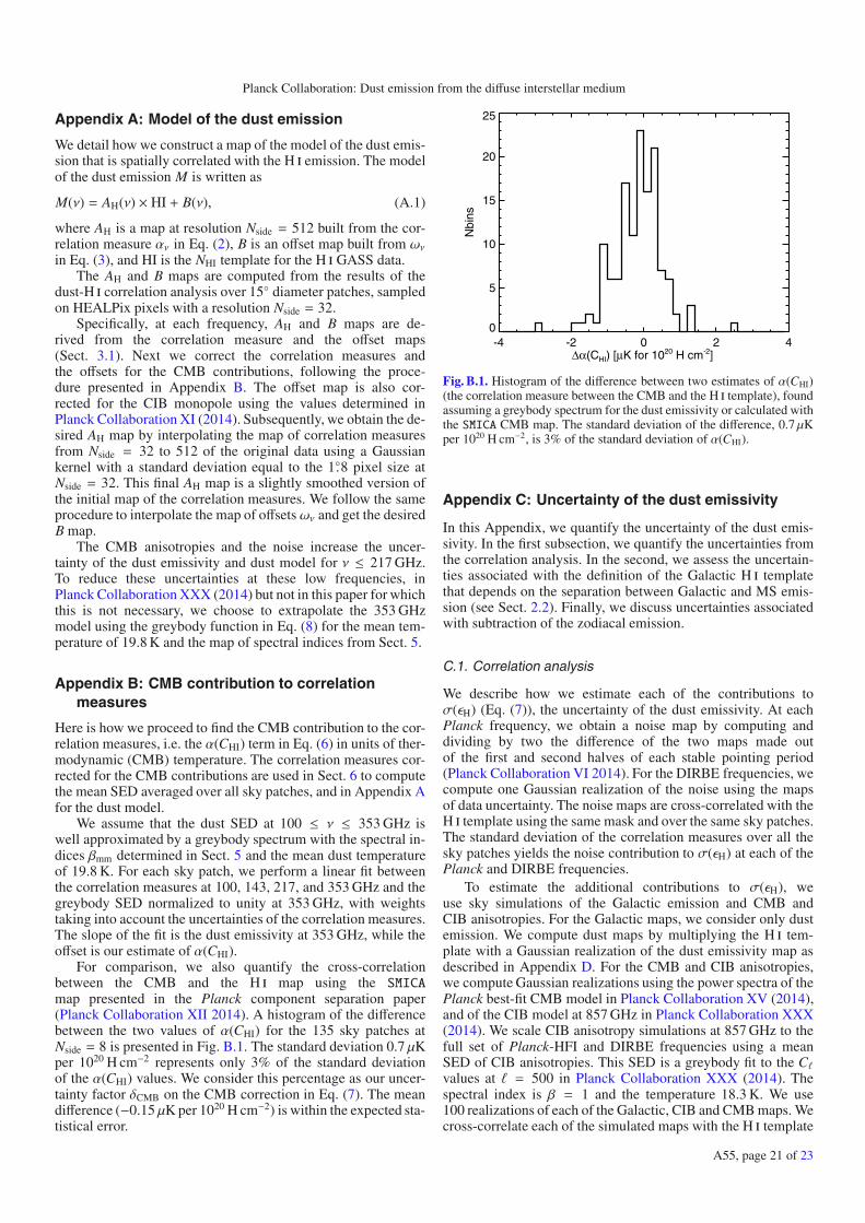
Planck Collaboration: Dust emission from the diffuse interstellar medium

Appendix A: Model of the dust emission

We detail how we construct a map of the model of the dust emis-sion that is spatially correlated with the H i emission. The modelof the dust emission M is written as

M(ν) = AH(ν) × HI + B(ν), (A.1)

where AH is a map at resolution Nside = 512 built from the cor-relation measure αν in Eq. (2), B is an offset map built from ωνin Eq. (3), and HI is the NHI template for the H i GASS data.

The AH and B maps are computed from the results of thedust-H i correlation analysis over 15◦ diameter patches, sampledon HEALPix pixels with a resolution Nside = 32.

Specifically, at each frequency, AH and B maps are de-rived from the correlation measure and the offset maps(Sect. 3.1). Next we correct the correlation measures andthe offsets for the CMB contributions, following the proce-dure presented in Appendix B. The offset map is also cor-rected for the CIB monopole using the values determined inPlanck Collaboration XI (2014). Subsequently, we obtain the de-sired AH map by interpolating the map of correlation measuresfrom Nside = 32 to 512 of the original data using a Gaussiankernel with a standard deviation equal to the 1.◦8 pixel size atNside = 32. This final AH map is a slightly smoothed version ofthe initial map of the correlation measures. We follow the sameprocedure to interpolate the map of offsets ων and get the desiredB map.

The CMB anisotropies and the noise increase the uncer-tainty of the dust emissivity and dust model for ν ≤ 217 GHz.To reduce these uncertainties at these low frequencies, inPlanck Collaboration XXX (2014) but not in this paper for whichthis is not necessary, we choose to extrapolate the 353 GHzmodel using the greybody function in Eq. (8) for the mean tem-perature of 19.8 K and the map of spectral indices from Sect. 5.

Appendix B: CMB contribution to correlationmeasures

Here is how we proceed to find the CMB contribution to the cor-relation measures, i.e. the α(CHI) term in Eq. (6) in units of ther-modynamic (CMB) temperature. The correlation measures cor-rected for the CMB contributions are used in Sect. 6 to computethe mean SED averaged over all sky patches, and in Appendix Afor the dust model.

We assume that the dust SED at 100 ≤ ν ≤ 353 GHz iswell approximated by a greybody spectrum with the spectral in-dices βmm determined in Sect. 5 and the mean dust temperatureof 19.8 K. For each sky patch, we perform a linear fit betweenthe correlation measures at 100, 143, 217, and 353 GHz and thegreybody SED normalized to unity at 353 GHz, with weightstaking into account the uncertainties of the correlation measures.The slope of the fit is the dust emissivity at 353 GHz, while theoffset is our estimate of α(CHI).

For comparison, we also quantify the cross-correlationbetween the CMB and the H i map using the SMICAmap presented in the Planck component separation paper(Planck Collaboration XII 2014). A histogram of the differencebetween the two values of α(CHI) for the 135 sky patches atNside = 8 is presented in Fig. B.1. The standard deviation 0.7 μKper 1020 H cm−2 represents only 3% of the standard deviationof the α(CHI) values. We consider this percentage as our uncer-tainty factor δCMB on the CMB correction in Eq. (7). The meandifference (−0.15 μK per 1020 H cm−2) is within the expected sta-tistical error.

-4 -2 0 2 4Δα(CHI) [μK for 1020 H cm-2]

0

5

10

15

20

25

Nbi

ns

Fig. B.1. Histogram of the difference between two estimates of α(CHI)(the correlation measure between the CMB and the H i template), foundassuming a greybody spectrum for the dust emissivity or calculated withthe SMICA CMB map. The standard deviation of the difference, 0.7μKper 1020 H cm−2, is 3% of the standard deviation of α(CHI).

Appendix C: Uncertainty of the dust emissivity

In this Appendix, we quantify the uncertainty of the dust emis-sivity. In the first subsection, we quantify the uncertainties fromthe correlation analysis. In the second, we assess the uncertain-ties associated with the definition of the Galactic H i templatethat depends on the separation between Galactic and MS emis-sion (see Sect. 2.2). Finally, we discuss uncertainties associatedwith subtraction of the zodiacal emission.

C.1. Correlation analysis

We describe how we estimate each of the contributions toσ(εH) (Eq. (7)), the uncertainty of the dust emissivity. At eachPlanck frequency, we obtain a noise map by computing anddividing by two the difference of the two maps made outof the first and second halves of each stable pointing period(Planck Collaboration VI 2014). For the DIRBE frequencies, wecompute one Gaussian realization of the noise using the mapsof data uncertainty. The noise maps are cross-correlated with theH i template using the same mask and over the same sky patches.The standard deviation of the correlation measures over all thesky patches yields the noise contribution to σ(εH) at each of thePlanck and DIRBE frequencies.

To estimate the additional contributions to σ(εH), weuse sky simulations of the Galactic emission and CMB andCIB anisotropies. For the Galactic maps, we consider only dustemission. We compute dust maps by multiplying the H i tem-plate with a Gaussian realization of the dust emissivity map asdescribed in Appendix D. For the CMB and CIB anisotropies,we compute Gaussian realizations using the power spectra of thePlanck best-fit CMB model in Planck Collaboration XV (2014),and of the CIB model at 857 GHz in Planck Collaboration XXX(2014). We scale CIB anisotropy simulations at 857 GHz to thefull set of Planck-HFI and DIRBE frequencies using a meanSED of CIB anisotropies. This SED is a greybody fit to the C�values at � = 500 in Planck Collaboration XXX (2014). Thespectral index is β = 1 and the temperature 18.3 K. We use100 realizations of each of the Galactic, CIB and CMB maps. Wecross-correlate each of the simulated maps with the H i template

A55, page 21 of 23

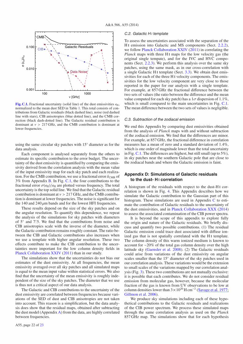
A&A 566, A55 (2014)

100 1000ν [GHz]

0.001

0.010

0.100

σ (ε

H)/

ε H

CMB

CIB

Data Noise

Galactic Residuals

Fig. C.1. Fractional uncertainty (solid line) of the dust emissivities εH,normalized to the mean dust SED in Table 1. This total consists of con-tributions from Galactic residuals (black dashed line), noise (red dashedline with stars), CIB anisotropies (blue dotted line), and the CMB cor-rection (black dash-dotted line). The Galactic residual contribution isdominant at ν > 217 GHz, and the CMB contribution is dominant atlower frequencies.

using the same circular sky patches with 15◦ diameter as for thedata analysis.

Each component is analysed separately from the others toestimate its specific contribution to the error budget. The uncer-tainty of the dust emissivity is quantified by comparing the emis-sivity derived from the correlation analysis with the mean valueof the input emissivity map for each sky patch and each realiza-tion. For the CMB contribution, we use a fractional error δCMB of3% from Appendix B. In Fig. C.1, the four contributions to thefractional error σ(εH)/εH are plotted versus frequency. The totaluncertainty is the top solid line. We find that the Galactic residualcontribution is dominant at ν > 217 GHz, and the CMB contribu-tion is dominant at lower frequencies. The noise is significant forthe 140 and 240 μm bands and for the lowest HFI frequencies.

These results depend on the size of the sky patches and onthe angular resolution. To quantify this dependence, we repeatthe analysis of the simulations for sky patches with diametersof 5◦ and 7.◦5. We find that the contributions from noise andCIB anisotropies scale with the inverse of the diameter, whilethe Galactic contribution remains roughly constant. The ratio be-tween the CIB and Galactic contributions also increases whenwe use a template with higher angular resolution. These twoeffects contribute to make the CIB contribution to the uncer-tainties more important for the low column density fields inPlanck Collaboration XXIV (2011) than in our study.

The simulations show that the uncertainties do not bias ourestimates of the dust emissivity. At all frequencies, the meanemissivity averaged over all sky patches and all simulated mapsis equal to the mean input value within statistical errors. We alsofind that the uncertainty of the mean emissivity is roughly inde-pendent of the size of the sky patches. The diameter that we useis thus not a critical aspect of our data analysis.

The Galactic and CIB contributions to the uncertainty of thedust emissivity are correlated between frequencies because vari-ations of the SED of dust and CIB anisotropies are not takeninto account. This reason is a simplification, but the data analy-sis does show that the residual maps, obtained after subtractingthe dust model (Appendix A) from the data, are highly correlatedbetween frequencies.

C.2. Galactic H I template

To assess the uncertainties associated with the separation of theH i emission into Galactic and MS components (Sect. 2.2.2),we follow Planck Collaboration XXIV (2011) in correlating thePlanck maps with three H i maps for the low velocity gas (theoriginal single tempate), and for the IVC and HVC compo-nents (Sect. 2.2.3). We perform this analysis over the same skypatches, using the same mask, as in our cross-correlation witha single Galactic H i template (Sect. 3.3). We obtain dust emis-sivities for each of the three H i velocity components. The emis-sivities for the low velocity component are very close to thosereported in the paper for our analysis with a single template.For example, at 857 GHz the fractional difference between thetwo sets of values (the ratio between the difference and the meanvalue computed for each sky patch) has a 1σ dispersion of 1.1%,which is small compared to the main uncertainties in Fig. C.1.The mean difference between the two sets of values is negligible.

C.3. Subtraction of the zodiacal emission

We end this Appendix by comparing dust emissivities obtainedfrom the analysis of Planck maps with and without subtractionof the zodiacal emission. We find that the differences are minor.For example, at 857 GHz, the fractional difference in correlationmeasures has a mean of zero and a standard deviation of 1.4%,which is one order of magnitude lower than the total uncertaintyin Fig. C.1. The differences are highest, but still small (up to 5%),in sky patches near the southern Galactic pole that are close tothe zodiacal bands and where the Galactic emission is faint.

Appendix D: Simulations of Galactic residualsto the dust- H I correlation

A histogram of the residuals with respect to the dust-H i cor-relation is shown in Fig. 4. This Appendix describes how wesimulate the Galactic contribution to the Gaussian part of thishistogram. These simulations are used in Appendix C to esti-mate the contribution of Galactic residuals to the uncertainty ofthe dust emissivities, and in Planck Collaboration XXX (2014)to assess the associated contamination of the CIB power spectra.

It is beyond the scope of this appendix to explore fullythe origin and nature of the Galactic residuals. We briefly dis-cuss and quantify two possible contributions. (1) The residualGalactic emission could trace dust associated with diffuse ion-ized gas that is not spatially correlated with the H i template.The column density of this warm ionized medium is known toaccount for ∼20% of the total gas column density over the highlatitude sky (Gaensler et al. 2008). (2) The Galactic residualscould arise from variations of the dust emissivity on angularscales smaller than the 15◦ diameter of the sky patches used inour correlation analysis. These variations would be the extensionto small scales of the variations mapped by our correlation anal-ysis (Fig. 3). These two contributions are not mutually exclusive:it is possible that each contributes. We do not consider residualemission from molecular gas, however, because the molecularfraction of the gas is known from UV observations to be low atcolumn densities lower than 3×1020 H cm−2 (Savage et al. 1977;Gillmon et al. 2006).

We produce sky simulations including each of these hypo-thetical contributions to the Galactic residuals and realizationsof the CIB power spectrum. We process these simulated mapsthrough the same correlation analysis as used on the Planck857 GHz map. The simulations show that for each hypothesis

A55, page 22 of 23

Planck Collaboration: Dust emission from the diffuse interstellar medium

we can match the amplitude and scatter of the values of σ857in Fig. 7; however, it is only when the simulated maps includesignificant variations in the dust emissivity that the simulationsmatch the systematic trend of σ857 growing with increasing NHI.We find that simulations can account for the main statisticalproperties of the Galactic residuals at 857 GHz when the map ofvariable dust emissivty is a Gaussian realization of a k−2.8 powerspectrum, without needing any contribution from the warmionized medium. The map of the dust emissivity is normalized to

reproduce the mean value and the standard deviation measuredfrom the correlation of the 857 GHz map and the H i template.We make multiple realizations of this specific model that areused in Appendix C and Planck Collaboration XXX (2014). Thesimulated maps at 857 GHz are scaled to other frequencies us-ing the mean SED in Table 1. The simulations do not take intoaccount the anti-correlation between the dust temperature andopacity.

A55, page 23 of 23