Planck 2013 results. XI. All-sky model of thermal dust emission

A&A 571, A11 (2014)DOI: 10.1051/0004-6361/201323195c© ESO 2014

Astronomy&

AstrophysicsPlanck 2013 results Special feature

Planck 2013 results. XI. All-sky model of thermal dust emissionPlanck Collaboration: A. Abergel62, P. A. R. Ade90, N. Aghanim62, M. I. R. Alves62, G. Aniano62, C. Armitage-Caplan95, M. Arnaud75,

M. Ashdown72,6, F. Atrio-Barandela19, J. Aumont62, C. Baccigalupi89, A. J. Banday98,9, R. B. Barreiro69, J. G. Bartlett1,70, E. Battaner100,K. Benabed63,97, A. Benoît60, A. Benoit-Lévy26,63,97, J.-P. Bernard98,9, M. Bersanelli36,51, P. Bielewicz98,9,89, J. Bobin75, J. J. Bock70,10,

A. Bonaldi71, J. R. Bond8, J. Borrill13,92, F. R. Bouchet63,97, F. Boulanger62, M. Bridges72,6,66, M. Bucher1, C. Burigana50,34, R. C. Butler50,J.-F. Cardoso76,1,63, A. Catalano77,74, A. Chamballu75,15,62, R.-R. Chary59, H. C. Chiang29,7, L.-Y Chiang65, P. R. Christensen84,39, S. Church94,M. Clemens46, D. L. Clements58, S. Colombi63,97, L. P. L. Colombo25,70, C. Combet77, F. Couchot73, A. Coulais74, B. P. Crill70,85, A. Curto6,69,F. Cuttaia50, L. Danese89, R. D. Davies71, R. J. Davis71, P. de Bernardis35, A. de Rosa50, G. de Zotti46,89, J. Delabrouille1, J.-M. Delouis63,97,

F.-X. Désert55, C. Dickinson71, J. M. Diego69, H. Dole62,61, S. Donzelli51, O. Doré70,10, M. Douspis62, B. T. Draine87, X. Dupac41, G. Efstathiou66,T. A. Enßlin80, H. K. Eriksen67, E. Falgarone74, F. Finelli50,52, O. Forni98,9, M. Frailis48, A. A. Fraisse29, E. Franceschi50, S. Galeotta48, K. Ganga1,

T. Ghosh62, M. Giard98,9, G. Giardino42, Y. Giraud-Héraud1, J. González-Nuevo69,89, K. M. Górski70,101, S. Gratton72,66, A. Gregorio37,48,54,I. A. Grenier75, A. Gruppuso50, V. Guillet62, F. K. Hansen67, D. Hanson81,70,8, D. L. Harrison66,72, G. Helou10, S. Henrot-Versillé73,

C. Hernández-Monteagudo12,80, D. Herranz69, S. R. Hildebrandt10, E. Hivon63,97, M. Hobson6, W. A. Holmes70, A. Hornstrup16, W. Hovest80,K. M. Huffenberger27, A. H. Jaffe58, T. R. Jaffe98,9, J. Jewell70, G. Joncas18, W. C. Jones29, M. Juvela28, E. Keihänen28, R. Keskitalo23,13,

T. S. Kisner79, J. Knoche80, L. Knox30, M. Kunz17,62,3, H. Kurki-Suonio28,44, G. Lagache62, A. Lähteenmäki2,44, J.-M. Lamarre74, A. Lasenby6,72,R. J. Laureijs42, C. R. Lawrence70, R. Leonardi41, J. León-Tavares43,2, J. Lesgourgues96,88, F. Levrier74, M. Liguori33, P. B. Lilje67,

M. Linden-Vørnle16, M. López-Caniego69, P. M. Lubin31, J. F. Macías-Pérez77, B. Maffei71, D. Maino36,51, N. Mandolesi50,5,34, M. Maris48,D. J. Marshall75, P. G. Martin8, E. Martínez-González69, S. Masi35, M. Massardi49, S. Matarrese33, F. Matthai80, P. Mazzotta38, P. McGehee59,A. Melchiorri35,53, L. Mendes41, A. Mennella36,51, M. Migliaccio66,72, S. Mitra57,70, M.-A. Miville-Deschênes62,8,∗, A. Moneti63, L. Montier98,9,

G. Morgante50, D. Mortlock58, D. Munshi90, J. A. Murphy83, P. Naselsky84,39, F. Nati35, P. Natoli34,4,50, C. B. Netterfield21,H. U. Nørgaard-Nielsen16, F. Noviello71, D. Novikov58, I. Novikov84, S. Osborne94, C. A. Oxborrow16, F. Paci89, L. Pagano35,53, F. Pajot62,

R. Paladini59, D. Paoletti50,52, F. Pasian48, G. Patanchon1, O. Perdereau73, L. Perotto77, F. Perrotta89, F. Piacentini35, M. Piat1, E. Pierpaoli25,D. Pietrobon70, S. Plaszczynski73, E. Pointecouteau98,9, G. Polenta4,47, N. Ponthieu62,55, L. Popa64, T. Poutanen44,28,2, G. W. Pratt75,

G. Prézeau10,70, S. Prunet63,97, J.-L. Puget62, J. P. Rachen22,80, W. T. Reach99, R. Rebolo68,14,40, M. Reinecke80, M. Remazeilles71,62,1, C. Renault77,S. Ricciardi50, T. Riller80, I. Ristorcelli98,9, G. Rocha70,10, C. Rosset1, G. Roudier1,74,70, M. Rowan-Robinson58, J. A. Rubiño-Martín68,40,B. Rusholme59, M. Sandri50, D. Santos77, G. Savini86, D. Scott24, M. D. Seiffert70,10, E. P. S. Shellard11, L. D. Spencer90, J.-L. Starck75,

V. Stolyarov6,72,93, R. Stompor1, R. Sudiwala90, R. Sunyaev80,91, F. Sureau75, D. Sutton66,72, A.-S. Suur-Uski28,44, J.-F. Sygnet63, J. A. Tauber42,D. Tavagnacco48,37, L. Terenzi50, L. Toffolatti20,69, M. Tomasi51, M. Tristram73, M. Tucci17,73, J. Tuovinen82, M. Türler56, G. Umana45,

L. Valenziano50, J. Valiviita44,28,67, B. Van Tent78, L. Verstraete62, P. Vielva69, F. Villa50, N. Vittorio38, L. A. Wade70, B. D. Wandelt63,97,32,N. Welikala1, N. Ysard28, D. Yvon15, A. Zacchei48, and A. Zonca31

(Affiliations can be found after the references)

Received 4 December 2013 / Accepted 4 September 2014

ABSTRACT

This paper presents an all-sky model of dust emission from the Planck 353, 545, and 857 GHz, and IRAS 100 µm data. Using a modified blackbodyfit to the data we present all-sky maps of the dust optical depth, temperature, and spectral index over the 353–3000 GHz range. This model is a goodrepresentation of the IRAS and Planck data at 5′ between 353 and 3000 GHz (850 and 100 µm). It shows variations of the order of 30% comparedwith the widely-used model of Finkbeiner, Davis, and Schlegel. The Planck data allow us to estimate the dust temperature uniformly over thewhole sky, down to an angular resolution of 5′, providing an improved estimate of the dust optical depth compared to previous all-sky dust model,especially in high-contrast molecular regions where the dust temperature varies strongly at small scales in response to dust evolution, extinction,and/or local production of heating photons. An increase of the dust opacity at 353 GHz, τ353/NH, from the diffuse to the denser interstellar medium(ISM) is reported. It is associated with a decrease in the observed dust temperature, Tobs, that could be due at least in part to the increaseddust opacity. We also report an excess of dust emission at H column densities lower than 1020 cm−2 that could be the signature of dust in thewarm ionized medium. In the diffuse ISM at high Galactic latitude, we report an anticorrelation between τ353/NH and Tobs while the dust specificluminosity, i.e., the total dust emission integrated over frequency (the radiance) per hydrogen atom, stays about constant, confirming one of thePlanck Early Results obtained on selected fields. This effect is compatible with the view that, in the diffuse ISM, Tobs responds to spatial variationsof the dust opacity, due to variations of dust properties, in addition to (small) variations of the radiation field strength. The implication is that inthe diffuse high-latitude ISM τ353 is not as reliable a tracer of dust column density as we conclude it is in molecular clouds where the correlationof τ353 with dust extinction estimated using colour excess measurements on stars is strong. To estimate Galactic E(B− V) in extragalactic fields athigh latitude we develop a new method based on the thermal dust radiance, instead of the dust optical depth, calibrated to E(B−V) using reddeningmeasurements of quasars deduced from Sloan Digital Sky Survey data.

Key words. methods: data analysis – ISM: general – dust, extinction – infrared: ISM – submillimeter: ISM – opacity

∗ Corresponding author: Marc-Antoine Miville-Deschênes, e-mail: [email protected]

Article published by EDP Sciences A11, page 1 of 37

A&A 571, A11 (2014)

1. Introduction

This paper, one of a set associated with the 2013 release ofdata from the Planck1 mission (Planck Collaboration I 2014),presents a new parametrization of dust emission that covers thewhole sky, at 5′ resolution, based on data from 353 to 3000 GHz(100 to 850 µm).

Because it is well mixed with the gas and because of its di-rect reaction to UV photons from stars, dust is a great tracer ofthe interstellar medium (ISM) and of star formation activity. Onthe other hand, for many studies in extragalactic astrophysicsand cosmology, Galactic interstellar dust is a nuisance, a sourceof extinction and reddening for UV to near-infrared observationsand a contaminating emission in the infrared to millimetre wave-lengths. Thanks to the sensitivity, spectral coverage, and angularresolution of Planck, this model of dust emission brings newconstraints on the dust spectral energy distribution (SED), on itsvariations across the sky, and on the relationships between dustemission, dust extinction, and gas column density. In particular,this model of dust emission provides a new map of dust extinc-tion at 5′ resolution, aimed at helping extragalactic studies.

The emission in the submillimetre range arises from the big-ger dust grains that are in thermal equilibrium with the ambientradiation field. Thermal dust emission is influenced by a combi-nation of the dust column density, radiation field strength, anddust properties (size distribution, chemical composition, and thegrain structure). When the effect of the radiation field can be esti-mated (using the dust temperature as a probe) and the dust prop-erties assumed, the dust optical depth is possibly the most reli-able tracer of interstellar column density, and therefore of massfor objects at known distances. Dust optical depth is used to es-timate the mass of interstellar clumps and cores (Ossenkopf &Henning 1994) in particular with the higher resolution Herscheldata (Launhardt et al. 2013), to study the statistical propertiesof the ISM structure and its link with gravity, interstellar turbu-lence, and stellar feedback (Peretto et al. 2012; Kainulainen et al.2013), and as a way to sample the mass of the ISM in general(Planck Collaboration XIX 2011). The accuracy of these deter-minations depends on, among other things, the frequency rangeover which the dust spectrum is observed. The combination ofPlanck and IRAS data offers a new view on interstellar dust byallowing us to sample the dust spectrum from the Wien to theRayleigh-Jeans sides, at 5′ resolution over the whole sky.

Dust emission, with extinction and polarization, is a key el-ement to constrain the properties of interstellar dust (Draine &Li 2007; Compiègne et al. 2011). The dust emissivity (i.e., theamount of emission per unit of gas column density) and theshape of the dust SED provide information on the nature ofthe dust particles, in particular their structure, composition, andabundance, related to the dust-to-gas ratio.

Changes in the dust emissivity and the shape of the dustSED can be related to dust evolutionary processes. Interstellardust grains are thought to be the seeds from which larger par-ticles form in the ISM, up to planetesimals in circumstellar en-vironments (Brauer et al. 2008; Beckwith et al. 2000; Birnstielet al. 2012). This growth of solids can be followed in earlierphases of the star-formation process, at the protostellar phaseand even before, in molecular clouds and in the diffuse ISM.

1 Planck (http://www.esa.int/Planck) is a project of theEuropean Space Agency (ESA) with instruments provided by two sci-entific consortia funded by ESA member states (in particular the leadcountries France and Italy), with contributions from NASA (USA) andtelescope reflectors provided by a collaboration between ESA and a sci-entific consortium led and funded by Denmark.

Many studies have revealed increases of the dust emissivity with(column) density in molecular clouds accompanied by a de-crease in dust temperature (Stepnik et al. 2003; Schnee et al.2008; Planck Collaboration XXV 2011; Arab et al. 2012; Martinet al. 2012; Roy et al. 2013). One explanation is that grainstructure is changing through aggregation of smaller particles,enhancing the opacity (Köhler et al. 2011). Planck’s spectralcoverage allows us to model the big grain thermal emission, inparticular its spectral index that is related to the grain composi-tion and structure (Ormel et al. 2011; Meny et al. 2007; Köhleret al. 2012). Because of its full-sky coverage, Planck can also re-veal variations of the dust SED with environment, enabling us tobetter understand the evolutionary track of dust grains throughthe ISM phases.

Dust emission is one of the major foregrounds hampering thestudy of the cosmic microwave background (CMB). The ther-mal dust emission peaks at a frequency close to 2000 GHz butits emission is still a fair fraction of the CMB anisotropies in the20–200 GHz range where they are measured. This is even morethe case in polarization (Miville-Deschênes 2011). The modelof dust emission proposed by Finkbeiner et al. (1999) based ondata from previous satellite missions (IRAS and COBE) madean important contribution to the field, in guiding the design ofCMB experiments and in helping the data analysis by providinga spatial template and a spectral dependence of the dust emis-sion at CMB frequencies. It is still the basis of recent models ofGalactic foreground emission (Delabrouille et al. 2013). With itsfrequency coverage that bridges the gap between IRAS and theCMB range, its high sensitivity, and its better angular resolution,Planck offers the opportunity to develop a new model of thermaldust emission.

Estimating reddening and extinction by foreground interstel-lar dust is a major issue for observations of extragalactic objectsin the UV to near-infrared range. Major efforts have been madetoward producing sky maps that provide a way to correct for thechromatic extinction of light by Galactic interstellar dust on anyline of sight. First Burstein & Heiles (1978) used H as a proxyfor dust extinction by correlating integrated 21 cm line emis-sion with extinction estimated from galaxy counts. It was subse-quently discovered that H is not a reliable tracer of total columndensity NH for NH greater than a few 1020 cm−2 due to molec-ular gas contributions (Lebrun et al. 1982; Boulanger & Pérault1988; Désert et al. 1988; Heiles et al. 1988; Blitz et al. 1990;Reach et al. 1994; Boulanger et al. 1996). It was then proposedto use dust emission as a more direct way to estimate dust ex-tinction. By combining 100, 140, and 240 µm data (DIRBE andIRAS) Schlegel et al. (1998) produced an all-sky map of dust op-tical depth at 100 µm that was then calibrated into dust reddeningby correlating with colour excesses measured for galaxies. Thework presented here is the direct continuation of these studies.Like Schlegel et al. (1998) we also propose a map of E(B − V)based on a model of dust emission calibrated using colour excessmeasurements of extragalactic objects, here quasars.

The paper is organized as follows. The data used and thepreprocessing steps are presented in Sect. 2. The model of thedust emission, SED fit methodology, the exploration of potentialbiases, and the all-sky maps of dust parameters are describedin Sect. 3. The results of the Galactic dust model are analysedin Sect. 4. Sections 5 and 6 describe specifically how the dustemission model compares to other tracers of column density. ThePlanck dust products, the dust model maps, and the E(B−V) mapaimed at helping extragalactic studies to estimate Galactic ex-tinction are detailed in Sect. 7 and compared with similar prod-ucts in the literature. Concluding remarks are given in Sect. 8.

A11, page 2 of 37

Planck collaboration: Planck 2013 results. XI.

2. Data and preprocessing

The analysis presented here relies on the combination of thePlanck data from the HFI instrument at 857, 545, and 353 GHz(respectively 350, 550, and 850 µm) with the IRAS 100 µm(3000 GHz) data.

2.1. Planck data

For Planck we used the HFI 2013 delivery maps (PlanckCollaboration VI 2014), corrected for zodiacal emission (ZE –see Planck Collaboration XIV 2014). Each map was smoothedto a common resolution of 5′, assuming a Gaussian beam2.The 353 GHz map, natively built in units of KCMB, was trans-formed to MJy sr−1 using the conversion factor given by PlanckCollaboration IX (2014). The CMB anisotropies map providedby the SMICA algorithm (Planck Collaboration XII 2014), whichhas an angular resolution of 5′, was removed from each PlanckHFI map.

As shown in Planck Collaboration XIII (2014), 12CO and13CO rotational lines fall in each of the Planck HFI filters, ex-cept at 143 GHz. At 857 and 545 GHz the CO lines (J = 5 → 4and J = 4→ 3, respectively) are very faint compared to the dustemission and they are not considered here. On the other hand,emission from the 12CO J = 3 → 2 line was detected in the353 GHz band (Planck Collaboration XIII 2014). Nevertheless,this emission is still faint compared to the dust emission whereasthe noise on the Planck CO emission estimate in the 353 GHzband is quite high (see Planck Collaboration XIII 2014 for de-tails). The detection of the 12CO J = 3 → 2 line emission byPlanck is above 3σ for only 2.6% of the sky. When detectedabove 3σ, this emission is on average 2% of the 353 GHz spe-cific intensity. It contributes 5% or more of the 353 GHz specificintensity for only 0.3% of the sky. Given such a relatively smallcontribution we did not subtract CO emission from the data so asnot to compromise the 353 GHz map through the adverse impactof the noise of the 12CO J = 3→ 2 product.

2.2. The 100 µm map

The 100 µm map used in this analysis is a combination of theIRIS map (Miville-Deschênes & Lagache 2005) and the mapof Schlegel et al. (1998, hereafter SFD), both projected on theHEALPix3 grid (Górski et al. 2005) at Nside = 2048. BothIRIS and SFD maps were built by combining IRAS and DIRBE100 µm data. Nevertheless these two maps show differences atlarge scales due to the different assumptions used for the ZE re-moval. Miville-Deschênes & Lagache (2005) used the DIRBE100 µm map from which ZE was removed by the DIRBE team,using the model of Kelsall et al. (1998). On the other hand,Schlegel et al. (1998) used their own empirical approach to re-move ZE based on a scaling of the DIRBE 25 µm data. Becauseit is based on data and not on a model, the SFD correction iscloser to the complex structure of the ZE and provides a bet-ter result. This can be assessed by looking at the correlation ofthe IRIS and SFD maps with H in the diffuse areas of the sky(1 < NH < 2 × 1020 cm−2), as detailed in Appendix A.1. Theuncertainty of the slope of the correlation with NH and the stan-dard deviation of the residual is about 30% lower for the SFD

2 Each map was smoothed using a Gaussian beam of FWHM, fs, thatcomplements the native FWHM, fi (Table 1), of the map to bring it to

5′: fs =

√52 − f 2

i .3 http://healpix.sourceforge.net

map compared to the IRIS map. For that reason (and others de-scribed in Appendix A.1) we favour the use of the SFD map atlarge scales.

At scales smaller than 30′, the IRIS map has several advan-tages over the SFD map4. The IRIS map is at the original angularresolution (4.′3) of the IRAS data while SFD smoothed the mapto 6.′1. IRIS also benefits from a non-linear gain correction thatis coherent for point sources and diffuse emission. Finally pointsources were kept in the IRIS map whereas SFD removed someof them (mostly galaxies but also ISM clumps). To combine theadvantages of the two maps, we built a 100 µm map, I100, thatis compatible with SFD at scales larger than 30′ and compatiblewith IRIS at smaller scales:

I100 = IIRIS − IIRIS ⊗ f 30IRIS + ISFD ⊗ f 30

SFD , (1)

where IIRIS and ISFD are, respectively, the IRIS and the SFDmaps, and f 30

i is the complementary Gaussian kernel needed tobring the maps to 30′ resolution.

2.3. Zero level

The fit of the dust emission requires that the specific intensityat each frequency and at each sky position is free of any otheremission. In particular the zero level of each map should be setin such a way that it contains only Galactic dust emission. Inorder to set the zero level of the maps to a meaningful Galacticreference we applied a method based on a correlation with H ,as described in Planck Collaboration VIII (2014).

Some precautions need to be taken here because the ratioof dust to H emission might vary locally due to variations ofthe radiation field or of the dust optical properties. Locally the21 cm emission might not be a perfect tracer of the column den-sity due to H self-absorption effects or to the presence of ion-ized or molecular gas. Nevertheless, the correlation between dustand H emission is known to be tight in the diffuse ISM wheremost of the gas is atomic. This correlation has been used sev-eral times to establish the dust SED (Boulanger et al. 1996;Planck Collaboration XXIV 2011), to isolate the cosmic infraredbackground (CIB; Puget et al. 1996; Planck Collaboration XVIII2011; Pénin et al. 2012), and to establish a Galactic reference fordust maps (Burstein & Heiles 1978; Schlegel et al. 1998).

The excess of dust emission with respect to the H correla-tion has been used to reveal gas in molecular form, even in re-gions where CO emission was not detected (Désert et al. 1988;Blitz et al. 1990; Reach et al. 1998; Planck Collaboration XIX2011). Such an excess can be observed at column densities aslow as NH = 2 × 1020 cm−2. Using this as an upper limit forour correlation studies also ensures that self-absorption in the21 cm line emission is not important. Note that this is also belowthe threshold at which significant H2 is seen in the diffuse ISM(Gillmon et al. 2006; Wakker 2006; Rachford et al. 2002, 2009).

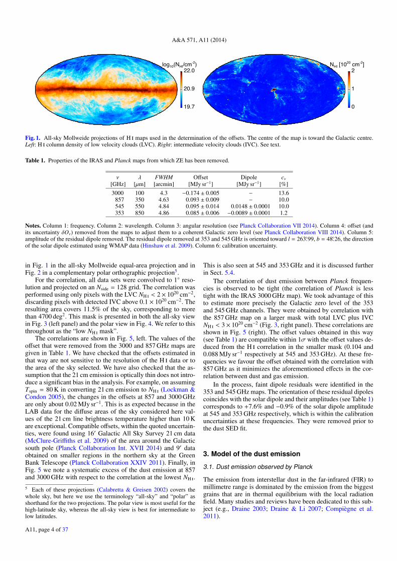
To estimate the Galactic reference of the IRAS and Planckdata, the maps were correlated against the 21 cm LAB data(Kalberla et al. 2005), integrated in velocity. The ranges are re-ferred to as LVC, low velocity gas with |vLSR| < 35 km s−1, andIVC, intermediate velocity gas with 35 < |vLSR| < 70 km s−1

(Albert & Danly 2004). HVC, high-velocity clouds with |vLSR| >70 km s−1 are excluded. For LVC and IVC separately, columndensity maps NH assuming optically thin emission are given

4 It is at 30′ that both maps match in power – see Fig. 15 ofMiville-Deschênes & Lagache (2005). This scale is close to the reso-lution of the DIRBE data (42′) that were used in both products to setthe large-scale emission.

A11, page 3 of 37

A&A 571, A11 (2014)

19.7

20.9

22.0log10(NHI/cm-2)

0

1

2NHI [1020 cm-2]

Fig. 1. All-sky Mollweide projections of H maps used in the determination of the offsets. The centre of the map is toward the Galactic centre.Left: H column density of low velocity clouds (LVC). Right: intermediate velocity clouds (IVC). See text.

Table 1. Properties of the IRAS and Planck maps from which ZE has been removed.

ν λ FWHM Offset Dipole cν[GHz] [µm] [arcmin] [MJy sr−1] [MJy sr−1] [%]3000 100 4.3 −0.174 ± 0.005 − 13.6

857 350 4.63 0.093 ± 0.009 − 10.0545 550 4.84 0.095 ± 0.014 0.0148 ± 0.0001 10.0353 850 4.86 0.085 ± 0.006 −0.0089 ± 0.0001 1.2

Notes. Column 1: frequency. Column 2: wavelength. Column 3: angular resolution (see Planck Collaboration VII 2014). Column 4: offset (andits uncertainty δOν) removed from the maps to adjust them to a coherent Galactic zero level (see Planck Collaboration VIII 2014). Column 5:amplitude of the residual dipole removed. The residual dipole removed at 353 and 545 GHz is oriented toward l = 263.◦99, b = 48.◦26, the directionof the solar dipole estimated using WMAP data (Hinshaw et al. 2009). Column 6: calibration uncertainty.

in Fig. 1 in the all-sky Mollweide equal-area projection and inFig. 2 in a complementary polar orthographic projection5.

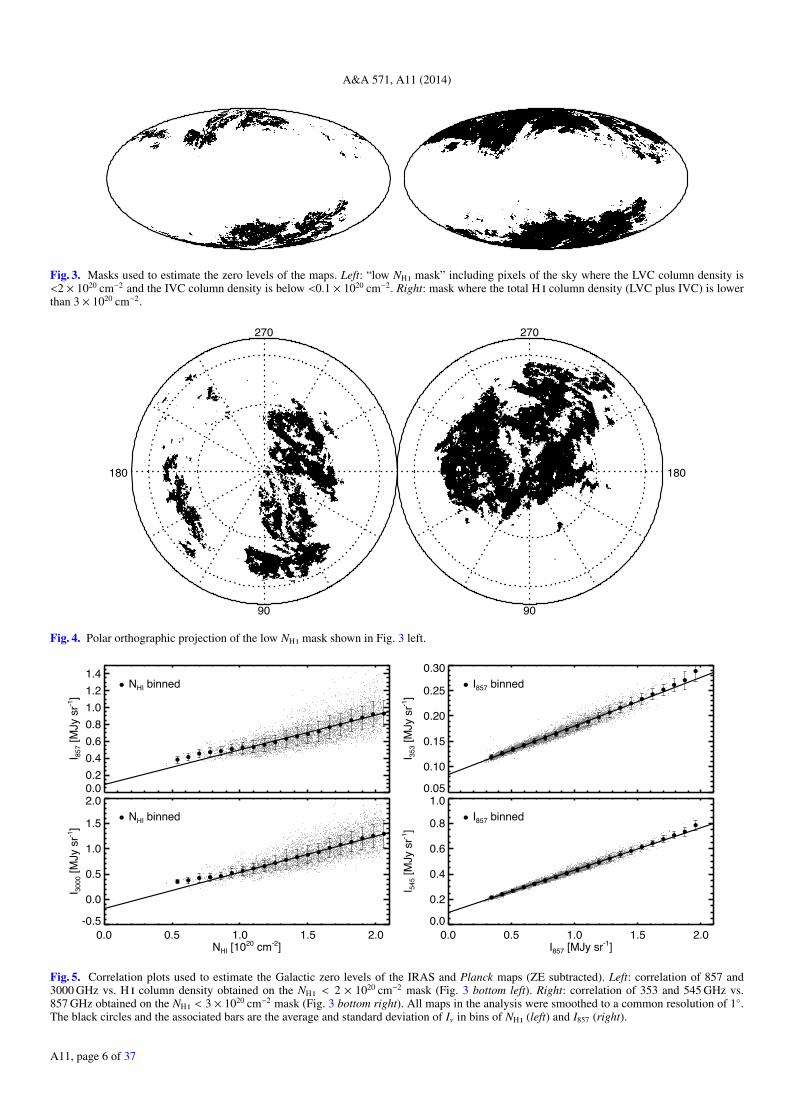
For the correlation, all data sets were convolved to 1◦ reso-lution and projected on an Nside = 128 grid. The correlation wasperformed using only pixels with the LVC NH < 2× 1020 cm−2,discarding pixels with detected IVC above 0.1 × 1020 cm−2. Theresulting area covers 11.5% of the sky, corresponding to morethan 4700 deg2. This mask is presented in both the all-sky viewin Fig. 3 (left panel) and the polar view in Fig. 4. We refer to thisthroughout as the “low NH mask”.

The correlations are shown in Fig. 5, left. The values of theoffset that were removed from the 3000 and 857 GHz maps aregiven in Table 1. We have checked that the offsets estimated inthat way are not sensitive to the resolution of the H data or tothe area of the sky selected. We have also checked that the as-sumption that the 21 cm emission is optically thin does not intro-duce a significant bias in the analysis. For example, on assumingTspin = 80 K in converting 21 cm emission to NH (Lockman &Condon 2005), the changes in the offsets at 857 and 3000 GHzare only about 0.02 MJy sr−1. This is as expected because in theLAB data for the diffuse areas of the sky considered here val-ues of the 21 cm line brightness temperature higher than 10 Kare exceptional. Compatible offsets, within the quoted uncertain-ties, were found using 16′ Galactic All Sky Survey 21 cm data(McClure-Griffiths et al. 2009) of the area around the Galacticsouth pole (Planck Collaboration Int. XVII 2014) and 9′ dataobtained on smaller regions in the northern sky at the GreenBank Telescope (Planck Collaboration XXIV 2011). Finally, inFig. 5 we note a systematic excess of the dust emission at 857and 3000 GHz with respect to the correlation at the lowest NH .

5 Each of these projections (Calabretta & Greisen 2002) covers thewhole sky, but here we use the terminology “all-sky” and “polar” asshorthand for the two projections. The polar view is most useful for thehigh-latitude sky, whereas the all-sky view is best for intermediate tolow latitudes.

This is also seen at 545 and 353 GHz and it is discussed furtherin Sect. 5.4.

The correlation of dust emission between Planck frequen-cies is observed to be tight (the correlation of Planck is lesstight with the IRAS 3000 GHz map). We took advantage of thisto estimate more precisely the Galactic zero level of the 353and 545 GHz channels. They were obtained by correlation withthe 857 GHz map on a larger mask with total LVC plus IVCNH < 3× 1020 cm−2 (Fig. 3, right panel). These correlations areshown in Fig. 5 (right). The offset values obtained in this way(see Table 1) are compatible within 1σ with the offset values de-duced from the H correlation in the smaller mask (0.104 and0.088 MJy sr−1 respectively at 545 and 353 GHz). At these fre-quencies we favour the offset obtained with the correlation with857 GHz as it minimizes the aforementioned effects in the cor-relation between dust and gas emission.

In the process, faint dipole residuals were identified in the353 and 545 GHz maps. The orientation of these residual dipolescoincides with the solar dipole and their amplitudes (see Table 1)corresponds to +7.6% and −0.9% of the solar dipole amplitudeat 545 and 353 GHz respectively, which is within the calibrationuncertainties at these frequencies. They were removed prior tothe dust SED fit.

3. Model of the dust emission

3.1. Dust emission observed by Planck

The emission from interstellar dust in the far-infrared (FIR) tomillimetre range is dominated by the emission from the biggestgrains that are in thermal equilibrium with the local radiationfield. Many studies and reviews have been dedicated to this sub-ject (e.g., Draine 2003; Draine & Li 2007; Compiègne et al.2011).

A11, page 4 of 37

Planck collaboration: Planck 2013 results. XI.

20

21

90

180

270

90

180

270

log10(NHI/cm-2)

0

1

2

90

180

270

90

180

270

NHI [1020 cm-2]

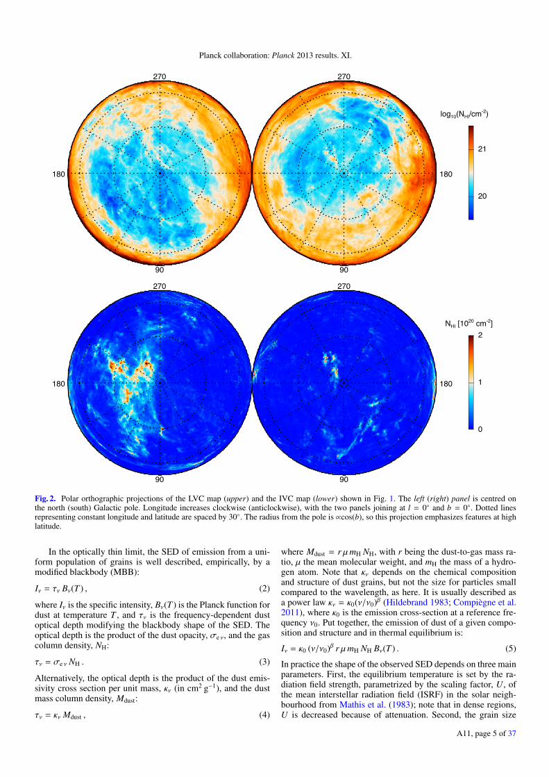
Fig. 2. Polar orthographic projections of the LVC map (upper) and the IVC map (lower) shown in Fig. 1. The left (right) panel is centred onthe north (south) Galactic pole. Longitude increases clockwise (anticlockwise), with the two panels joining at l = 0◦ and b = 0◦. Dotted linesrepresenting constant longitude and latitude are spaced by 30◦. The radius from the pole is ∝cos(b), so this projection emphasizes features at highlatitude.

In the optically thin limit, the SED of emission from a uni-form population of grains is well described, empirically, by amodified blackbody (MBB):

Iν = τν Bν(T ) , (2)

where Iν is the specific intensity, Bν(T ) is the Planck function fordust at temperature T , and τν is the frequency-dependent dustoptical depth modifying the blackbody shape of the SED. Theoptical depth is the product of the dust opacity, σe ν, and the gascolumn density, NH:

τν = σe ν NH . (3)

Alternatively, the optical depth is the product of the dust emis-sivity cross section per unit mass, κν (in cm2 g−1), and the dustmass column density, Mdust:

τν = κν Mdust , (4)

where Mdust = r µmH NH, with r being the dust-to-gas mass ra-tio, µ the mean molecular weight, and mH the mass of a hydro-gen atom. Note that κν depends on the chemical compositionand structure of dust grains, but not the size for particles smallcompared to the wavelength, as here. It is usually described asa power law κν = κ0(ν/ν0)β (Hildebrand 1983; Compiègne et al.2011), where κ0 is the emission cross-section at a reference fre-quency ν0. Put together, the emission of dust of a given compo-sition and structure and in thermal equilibrium is:

Iν = κ0 (ν/ν0)β r µmH NH Bν(T ) . (5)

In practice the shape of the observed SED depends on three mainparameters. First, the equilibrium temperature is set by the ra-diation field strength, parametrized by the scaling factor, U, ofthe mean interstellar radiation field (ISRF) in the solar neigh-bourhood from Mathis et al. (1983); note that in dense regions,U is decreased because of attenuation. Second, the grain size

A11, page 5 of 37

A&A 571, A11 (2014)

Fig. 3. Masks used to estimate the zero levels of the maps. Left: “low NH mask” including pixels of the sky where the LVC column density is<2 × 1020 cm−2 and the IVC column density is below <0.1 × 1020 cm−2. Right: mask where the total H column density (LVC plus IVC) is lowerthan 3 × 1020 cm−2.

90

180

270

90

180

270

Fig. 4. Polar orthographic projection of the low NH mask shown in Fig. 3 left.

0.0 0.5 1.0 1.5 2.0NHI [1020 cm-2]

-0.5

0.0

0.5

1.0

1.5

2.0NHI binned

I 3000

[MJy

sr-1

]

0.00.20.40.60.81.01.21.4

NHI binned

I 857 [

MJy

sr-1

]

0.0 0.5 1.0 1.5 2.0I857 [MJy sr-1]

0.0

0.2

0.4

0.6

0.8

1.0I857 binned

I 545 [

MJy

sr-1

]

0.05

0.10

0.15

0.20

0.25

0.30I857 binned

I 353 [

MJy

sr-1

]

Fig. 5. Correlation plots used to estimate the Galactic zero levels of the IRAS and Planck maps (ZE subtracted). Left: correlation of 857 and3000 GHz vs. H column density obtained on the NH < 2 × 1020 cm−2 mask (Fig. 3 bottom left). Right: correlation of 353 and 545 GHz vs.857 GHz obtained on the NH < 3 × 1020 cm−2 mask (Fig. 3 bottom right). All maps in the analysis were smoothed to a common resolution of 1◦.The black circles and the associated bars are the average and standard deviation of Iν in bins of NH (left) and I857 (right).

A11, page 6 of 37

Planck collaboration: Planck 2013 results. XI.

distribution (Mathis et al. 1977; Weingartner & Draine 2001) isimportant; exposed to the same ISRF, bigger grains have a lowerequilibrium temperature than smaller ones. Third, the dust struc-ture and composition determine not only the optical and UV ab-sorption cross section, but also the emission cross-section, thefrequency-dependent efficiency to emit radiation, usually mod-elled as above as a power law (κ0 ν

β) but possibly more com-plex depending on dust properties (β could vary with frequencyand/or grain size and/or grain temperature). In a given volumeelement along the line of sight, the distribution of dust grainsizes will naturally create a distribution of equilibrium temper-atures. In addition, dust properties might vary along the line ofsight. Furthermore, U might also change along some lines ofsight. Therefore, the observed dust SED is a mixture of emissionmodified by these effects, the sum of several different MBBs.Nevertheless, the simplification of fitting a single MBB is of-ten adopted and indeed here, with only four photometric bandsavailable, is unavoidable. The parametrization of the MBB forthe empirical fit is:

Iν = τν0 Bν(Tobs)(ν

ν0

)βobs

, (6)

where ν0 is a reference frequency at which the optical depth τν0 isestimated (ν0 = 353 GHz in our SED applications in this paper).

The main challenge is then to relate the parameters of thefit to physical quantities. It has been shown by many authors(Blain et al. 2003; Schnee et al. 2007; Shetty et al. 2009b; Kellyet al. 2012; Juvela & Ysard 2012a,b; Ysard et al. 2012) that, ingeneral, the values of Tobs and βobs recovered from an MBB fitcannot be related simply to the mass-weighted average along theline of sight of the dust temperature and spectral index. Evenfor dust with a spectral index constant in frequency (i.e., β doesnot depend on ν), the distribution of grain sizes and the varia-tions of U along the line of sight could introduce a broadeningof the SED relative to the case of a single dust size and sin-gle U. In addition, the dust luminosity is proportional to T 4+β

and so dust that is hotter for any reason, including efficiencyof absorption, will contribute more to the emission at all fre-quencies than colder dust. Therefore, the observed SED is not aquantity weighted by mass alone. The dust SED is wider than asingle MBB due to the distribution of T , and so the fit is boundto find a solution where βobs < β and, in consequence, whereTobs is biased toward higher values. This results in dust opti-cal depth that is generally underestimated: τobs < τ. This ef-fect is somewhat mitigated when lower frequency data are in-cluded. In the Rayleigh-Jeans limit the effect of temperature islow and the shape of the spectrum is dominated by the true β.For T = 15–25 K dust, this range is at frequencies lower thanν = k T/h = 310–520 GHz.

Models like the ones of Draine & Li (2007) and Compiègneet al. (2011) go beyond the simple MBB parametrization byincorporating the variation of the equilibrium temperature ofgrains due to the size distribution. The model of Draine & Li(2007) also includes a prescription for the variation of U alongthe line of sight, but assumes fixed dust properties. Nevertheless,there are still many uncertainties in the properties of dust (the ex-act size distribution of big grains, the optical properties, and thestructure of grains), in the evolution of these properties from dif-fuse to denser clouds, and in the variation of the radiation fieldstrength along the line of sight.

Therefore, for our early exploration of the dust SED over thewhole sky, at 5′ resolution and down to 353 GHz (850 µm), webelieve that it is useful to fit the dust SED using the empiricalMBB approach, before attempting to use more physical models

that rest on specific hypotheses. The three parameters τν0 , Tobsand βobs obtained from the MBB fit should be regarded as away to fit the data empirically; the complex relationship betweenthese recovered parameters and physical quantities needs to beinvestigated in detail with dedicated simulations (e.g., Ysardet al. 2012), but is beyond the scope of this paper.

3.2. Implementation of the SED fit

The fit of the dust SED with a MBB model has been carriedout traditionally using a χ2 minimization approach. Recently,alternative methods for fitting observational data with limitedspectral coverage have been proposed, based on Bayesian orhierarchical models (Veneziani et al. 2010, 2013; Kelly et al.2012; Juvela et al. 2013). These new methods were developedspecifically to limit the impact of instrumental noise on the es-timated parameters. Even though these methods offer interest-ing avenues, we developed our own strategy to fit the dust SEDover the whole sky because of another challenge to be mitigated,arising from the cosmic infrared background anisotropies (theCIBA). Although this has been overlooked, it can be dominantin the faint diffuse areas of the sky, as we demonstrate. We pro-ceeded with a method based on the standard χ2 minimization(see Appendix B) but implemented a two-step approach thatlimits the fluctuations of the estimated parameters at small an-gular scales induced by noise and the CIBA. In developing themethodology we have explored using data degraded to lower res-olution and smaller Nside.

3.2.1. Frequency coverageOne possible source of bias in the fit is the number of bandsand their central frequency. The combination of Planck 353 to857 GHz and IRIS 3000 GHz data allows us to sample the lowand high frequency sides of the dust SED. For a typical tem-perature of 20 K, the peak of the emission is at a frequency of2070 GHz. This falls in a gap in the frequency coverage, be-tween 857 GHz and 3000 GHz. It is thus a concern that a fit ofthe Planck and IRIS data might bias the recovered parametersTobs and βobs. To explore this we combined the Planck data withthe DIRBE data at 1250, 2143, and 3000 GHz (100, 140, and240 µm), all smoothed to 60′, providing a better sample of thedust SED near its peak. We found that the recovered dust param-eters are stable whether DIRBE data are used or not; no bias isobserved in Tobs, βobs, and τ353 compared with results obtainedusing just Planck and IRIS data.

We also evaluated the potential advantage of fitting the SEDwith only the Planck 353 to 857 GHz data, a more coherentdataset not relying on the IRIS data. However, because the Wienpart of the SED is not sampled the results showed a clear biasof Tobs, toward lower values; consequently, when extrapolatedto 100 µm, the fits greatly underestimate the emission detectedin the IRIS data. Therefore, in the following the χ2 minimiza-tion fit was carried out on the data described in Sect. 2: the 857,545, and 353 GHz Planck maps, corrected for zodiacal emission,and the new 100 µm map obtained by combining the IRIS andSFD maps.

3.2.2. Noise and cosmic infrared background anisotropies

Degeneracy (anticorrelation) of the estimated Tobs and βobs, in-herent to the MBB fit of dust emission in the presence of noise,has had dedicated specific study (Shetty et al. 2009a; Juvela &Ysard 2012a). As mentioned above, the CIBA is also a contam-inating source in the estimate of the MBB parameters.

A11, page 7 of 37

A&A 571, A11 (2014)

16 18 20 22 24 26 28Tobs [K]

0

0.01

0.02

0.03

0.04

0.05

ND

F

120’60’30’15’

5’

1.2 1.4 1.6 1.8 2.0 2.2 2.4`obs

0

0.01

0.02

0.03

0.04

NDF

120’60’30’15’5’

-6.6 -6.4 -6.2 -6.0 -5.8 -5.6 -5.4log10(o353)

0

0.01

0.02

0.03

NDF

120’60’30’15’5’

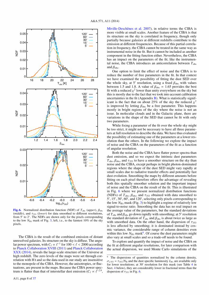
Fig. 6. Normalized distribution function (NDF) of Tobs (upper), βobs(middle), and τ353 (lower) for data smoothed to different resolutions,from 5′ to 2◦. The NDFs are shown only for the pixels correspondingto the low NH mask of Fig. 3, left, i.e., to the faintest 10% of the skypixels.

The CIBA is the result of the combined emission of distantunresolved galaxies. Its structure on the sky is diffuse. The angu-lar power spectrum, with C` ∝ `

−1 for 100 < ` < 2000 accordingto Planck Collaboration XVIII (2011) and Planck CollaborationXXX (2014), reveals the large-scale structure of the Universe athigh redshift. The zero levels of the maps were set through cor-relation with H and so the data used in our study are insensitiveto the monopole of the CIBA. However, the anisotropies, or fluc-tuations, are present in the maps. Because the CIBA power spec-trum is flatter than that of interstellar dust emission (C` ∝ `

−2.9,

Miville-Deschênes et al. 2007), in relative terms the CIBA ismore visible at small scales. Another feature of the CIBA is thatits structure on the sky is correlated in frequency, though onlypartially because galaxies at different redshifts contribute to theemission at different frequencies. Because of this partial correla-tion in frequency, the CIBA cannot be treated in the same way asinstrumental noise in the fit. But it cannot be included as anothercomponent in the fitting function either. Nevertheless, the CIBAhas an impact on the parameters of the fit; like the instrumen-tal noise, the CIBA introduces an anticorrelation between Tobsand βobs.

One option to limit the effect of noise and the CIBA is toreduce the number of free parameters in the fit. In that contextwe have examined the possibility of fitting the dust SED overthe whole sky, at 5′ resolution, using a fixed βobs with valuesbetween 1.5 and 1.8. A value of βobs = 1.65 provides the bestfit with a reduced χ2 lower than unity everywhere on the sky butthis is mostly due to the fact that we took into account calibrationuncertainties in the fit (Appendix B). What is statistically signif-icant is the fact that on about 25% of the sky the reduced χ2

is improved by letting βobs be a free parameter. This happensmostly in bright regions of the sky where the noise is not anissue. In molecular clouds and in the Galactic plane, there arevariations in the shape of the SED that cannot be fit with onlytwo parameters.

While fixing a parameter of the fit over the whole sky mightbe too strict, it might not be necessary to have all three parame-ters at full resolution to describe the data. We have thus evaluatedthe possibility of estimating one of the parameters at a lower res-olution than the others. In the following we explore the impactof noise and the CIBA on the parameters of the fit as a functionof angular resolution.

Both the noise and the CIBA have flatter power spectra thandust emission, and so we expect the intrinsic dust parametersTobs, βobs, and τ353 to have a smoother structure on the sky thannoise and the CIBA, except perhaps in bright photon-dominatedregions where the shape of the dust SED might vary rapidly atsmall scales due to radiative transfer effects and potentially fastdust evolution. Smoothing the maps by different amounts beforefitting on each pixel therefore offers the advantage of revealingboth this spatially smoother solution and the important impactof noise and the CIBA on the result of the fit. This is illustratedin Fig. 6 where we present normalized distribution functions(NDFs) of Tobs, βobs, and τ353 obtained with data smoothed to5′, 15′, 30′, 60′, and 120′, selecting only pixels corresponding tothe low NH mask (Fig. 3) to highlight a regime of relatively lowsignal-to-noise ratio. Smoothing the data has no real impact onthe average value of the parameters, but the standard deviationsof Tobs and βobs go down rapidly with smoothing; at 5′ resolutionthe standard deviation of Tobs and βobs is about twice as large aswith smoothed data. On the other hand, the dispersion of τ353is less affected by smoothing; it is dominated instead by cos-mic variance, the considerable range of column densities evenwithin this low NH mask6. Of course the dust parameters mightalso vary at small scales and so a trade-off needs to be found.

To explore and quantify the impact of noise and the CIBA onthe fit at different angular resolutions, for later comparison withthe actual dispersion, we used Monte Carlo simulations of the

6 The dispersions of quantities normalized by the column density,σe 353 = τ353/NH and the dust specific luminosity LH, are available onlyfor lower resolutions; at 30′ resolution for this mask (see Table 4 inSect. 4 below), they are considerably lower in fractional terms than thedispersion of τ353 in Fig. 6.

A11, page 8 of 37

Planck collaboration: Planck 2013 results. XI.

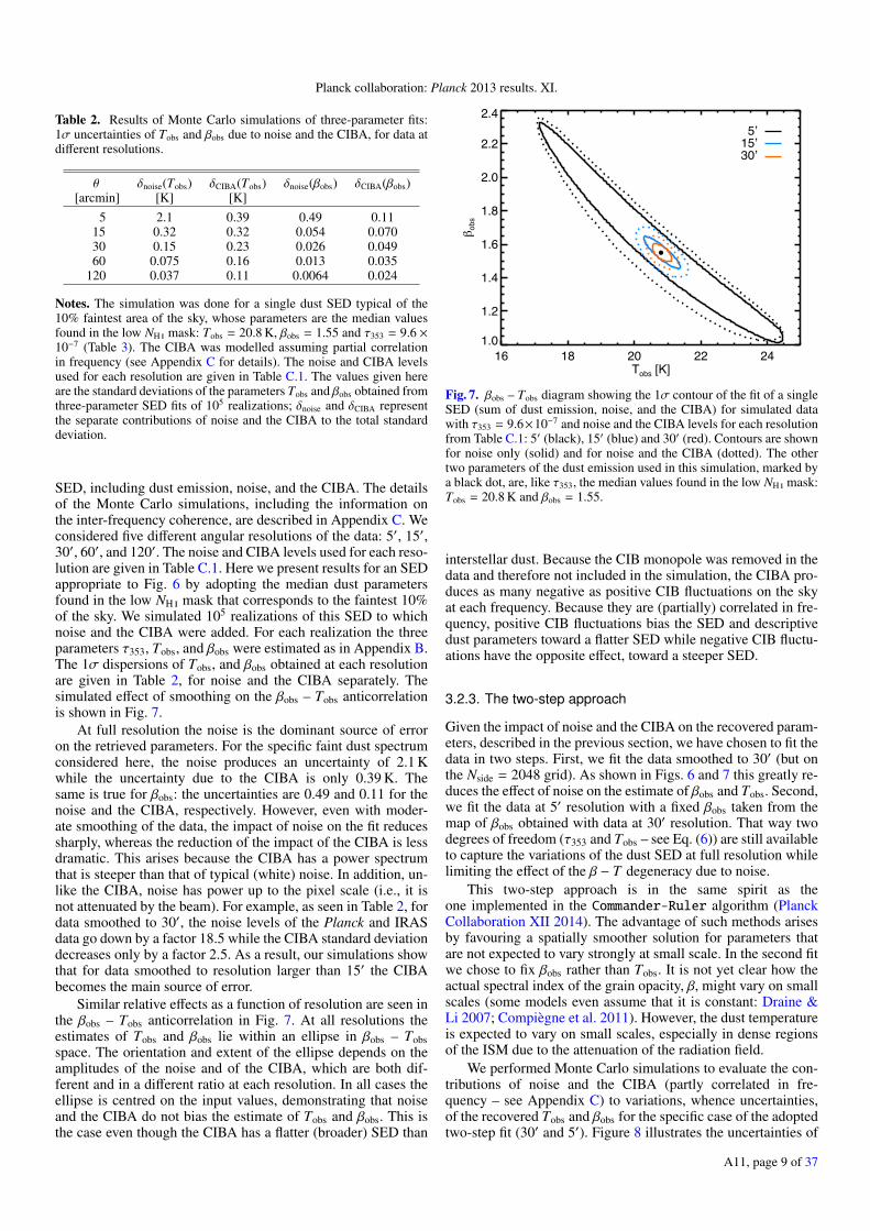
Table 2. Results of Monte Carlo simulations of three-parameter fits:1σ uncertainties of Tobs and βobs due to noise and the CIBA, for data atdifferent resolutions.

θ δnoise(Tobs) δCIBA(Tobs) δnoise(βobs) δCIBA(βobs)[arcmin] [K] [K]

5 2.1 0.39 0.49 0.1115 0.32 0.32 0.054 0.07030 0.15 0.23 0.026 0.04960 0.075 0.16 0.013 0.035

120 0.037 0.11 0.0064 0.024

Notes. The simulation was done for a single dust SED typical of the10% faintest area of the sky, whose parameters are the median valuesfound in the low NH mask: Tobs = 20.8 K, βobs = 1.55 and τ353 = 9.6 ×10−7 (Table 3). The CIBA was modelled assuming partial correlationin frequency (see Appendix C for details). The noise and CIBA levelsused for each resolution are given in Table C.1. The values given hereare the standard deviations of the parameters Tobs and βobs obtained fromthree-parameter SED fits of 105 realizations; δnoise and δCIBA representthe separate contributions of noise and the CIBA to the total standarddeviation.

SED, including dust emission, noise, and the CIBA. The detailsof the Monte Carlo simulations, including the information onthe inter-frequency coherence, are described in Appendix C. Weconsidered five different angular resolutions of the data: 5′, 15′,30′, 60′, and 120′. The noise and CIBA levels used for each reso-lution are given in Table C.1. Here we present results for an SEDappropriate to Fig. 6 by adopting the median dust parametersfound in the low NH mask that corresponds to the faintest 10%of the sky. We simulated 105 realizations of this SED to whichnoise and the CIBA were added. For each realization the threeparameters τ353, Tobs, and βobs were estimated as in Appendix B.The 1σ dispersions of Tobs, and βobs obtained at each resolutionare given in Table 2, for noise and the CIBA separately. Thesimulated effect of smoothing on the βobs – Tobs anticorrelationis shown in Fig. 7.

At full resolution the noise is the dominant source of erroron the retrieved parameters. For the specific faint dust spectrumconsidered here, the noise produces an uncertainty of 2.1 Kwhile the uncertainty due to the CIBA is only 0.39 K. Thesame is true for βobs: the uncertainties are 0.49 and 0.11 for thenoise and the CIBA, respectively. However, even with moder-ate smoothing of the data, the impact of noise on the fit reducessharply, whereas the reduction of the impact of the CIBA is lessdramatic. This arises because the CIBA has a power spectrumthat is steeper than that of typical (white) noise. In addition, un-like the CIBA, noise has power up to the pixel scale (i.e., it isnot attenuated by the beam). For example, as seen in Table 2, fordata smoothed to 30′, the noise levels of the Planck and IRASdata go down by a factor 18.5 while the CIBA standard deviationdecreases only by a factor 2.5. As a result, our simulations showthat for data smoothed to resolution larger than 15′ the CIBAbecomes the main source of error.

Similar relative effects as a function of resolution are seen inthe βobs – Tobs anticorrelation in Fig. 7. At all resolutions theestimates of Tobs and βobs lie within an ellipse in βobs – Tobsspace. The orientation and extent of the ellipse depends on theamplitudes of the noise and of the CIBA, which are both dif-ferent and in a different ratio at each resolution. In all cases theellipse is centred on the input values, demonstrating that noiseand the CIBA do not bias the estimate of Tobs and βobs. This isthe case even though the CIBA has a flatter (broader) SED than

16 18 20 22 24Tobs [K]

1.0

1.2

1.4

1.6

1.8

2.0

2.2

2.4

` obs

5’15’30’

Fig. 7. βobs – Tobs diagram showing the 1σ contour of the fit of a singleSED (sum of dust emission, noise, and the CIBA) for simulated datawith τ353 = 9.6×10−7 and noise and the CIBA levels for each resolutionfrom Table C.1: 5′ (black), 15′ (blue) and 30′ (red). Contours are shownfor noise only (solid) and for noise and the CIBA (dotted). The othertwo parameters of the dust emission used in this simulation, marked bya black dot, are, like τ353, the median values found in the low NH mask:Tobs = 20.8 K and βobs = 1.55.

interstellar dust. Because the CIB monopole was removed in thedata and therefore not included in the simulation, the CIBA pro-duces as many negative as positive CIB fluctuations on the skyat each frequency. Because they are (partially) correlated in fre-quency, positive CIB fluctuations bias the SED and descriptivedust parameters toward a flatter SED while negative CIB fluctu-ations have the opposite effect, toward a steeper SED.

3.2.3. The two-step approach

Given the impact of noise and the CIBA on the recovered param-eters, described in the previous section, we have chosen to fit thedata in two steps. First, we fit the data smoothed to 30′ (but onthe Nside = 2048 grid). As shown in Figs. 6 and 7 this greatly re-duces the effect of noise on the estimate of βobs and Tobs. Second,we fit the data at 5′ resolution with a fixed βobs taken from themap of βobs obtained with data at 30′ resolution. That way twodegrees of freedom (τ353 and Tobs – see Eq. (6)) are still availableto capture the variations of the dust SED at full resolution whilelimiting the effect of the β − T degeneracy due to noise.

This two-step approach is in the same spirit as theone implemented in the Commander-Ruler algorithm (PlanckCollaboration XII 2014). The advantage of such methods arisesby favouring a spatially smoother solution for parameters thatare not expected to vary strongly at small scale. In the second fitwe chose to fix βobs rather than Tobs. It is not yet clear how theactual spectral index of the grain opacity, β, might vary on smallscales (some models even assume that it is constant: Draine &Li 2007; Compiègne et al. 2011). However, the dust temperatureis expected to vary on small scales, especially in dense regionsof the ISM due to the attenuation of the radiation field.

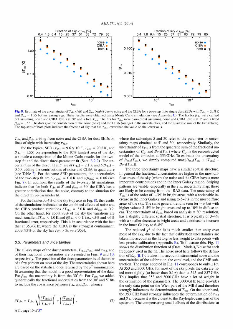
We performed Monte Carlo simulations to evaluate the con-tributions of noise and the CIBA (partly correlated in fre-quency – see Appendix C) to variations, whence uncertainties,of the recovered Tobs and βobs for the specific case of the adoptedtwo-step fit (30′ and 5′). Figure 8 illustrates the uncertainties of

A11, page 9 of 37

A&A 571, A11 (2014)

10-6 10-5

o353

0.01

0.10

1.00

bTob

s [K]

0.4 1.8 6.4 15 25 37 51 63 72 79 85Fraction of sky < o353 [%]

noiseCIBAboth

10-6 10-5

o353

0.001

0.010

0.100

b`ob

s

0.4 1.8 6.4 15 25 37 51 63 72 79 85Fraction of sky < o353 [%]

noiseCIBAboth

Fig. 8. Estimate of the uncertainties of Tobs (left) and βobs (right) due to noise and the CIBA for a two-step fit to single dust SEDs with Tobs = 20.8 Kand βobs = 1.55 but increasing τ353. These results were obtained using Monte Carlo simulations (see Appendix C). The fits for βobs were carriedout assuming noise and CIBA levels at 30′ and a free Tobs. The fits for Tobs were carried out assuming noise and CIBA levels at 5′ and a fixedβobs = 1.55. The dots give the contribution of the noise (blue) and the CIBA (orange) to the uncertainties, and the quadratic sum of the two (black).The top axes of both plots indicate the fraction of sky that has τ353 lower than the value on the lower axis.

Tobs and βobs arising from noise and the CIBA for dust SEDs onlines of sight with increasing τ353.

For the typical SED (τ353 = 9.6 × 10−7, Tobs = 20.8 K, andβobs = 1.55) corresponding to the 10% faintest area of the sky,we made a comparison of the Monte-Carlo results for the two-step fit and the direct three-parameter fit (Sect. 3.2.2). The un-certainties of the direct fit at 5′ are δ(Tobs) = 2.1 K and δ(βobs) =0.50, adding the contributions of noise and CIBA in quadrature(see Table 2). For the same SED parameters, the uncertaintiesof the two-step fit are δ(Tobs) = 0.8 K and δ(βobs) = 0.06 (seeFig. 8). In addition, the results of the two-step fit simulationsindicate that for both Tobs at 5′ and βobs at 30′ the CIBA has agreater contribution than the noise, contrary to the situation forthe direct three-parameter fit.

For the faintest 0.4% of the sky (top axis in Fig. 8), the resultsof the simulations indicate that the combined effects of noise andthe CIBA produce variations δTobs = 3.0 K and δβobs = 0.2.On the other hand, for about 93% of the sky the variations aremuch smaller, δTobs < 1.0 K and δβobs < 0.1, i.e., <5% and <6%fractional error, respectively. This is in accordance with the factthat at 353 GHz, where the CIBA is the strongest contaminant,about 93% of the sky has I353 > 3σCIBA(353).

3.3. Parameters and uncertainties

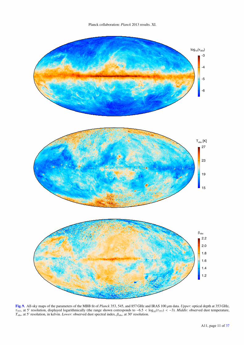
The all-sky maps of the dust parameters, Tobs, βobs, and τ353, andof their fractional uncertainties are presented in Figs. 9 and 10,respectively. The precision of the three parameters is of the orderof a few percent on most of the sky. The uncertainties shown hereare based on the statistical ones returned by the χ2 minimizationfit assuming that the model is a good representation of the data.For βobs the uncertainty is from the 30′ fit. For Tobs we addedquadratically the fractional uncertainties from the 30′ and 5′ fitsto include the covariance between Tobs and βobs, whence

δTobs = Tobs

√(δTobs,30

Tobs,30

)2

+

(δTobs,5

Tobs,5

)2

, (7)

where the subscripts 5 and 30 refer to the parameter or uncer-tainty maps obtained at 5′ and 30′, respectively. Similarly, theuncertainty of τ353 is from the quadratic sum of the fractional un-certainties of Im

353 and B353(Tobs) where Im353 is the reconstructed

model of the emission at 353 GHz. To estimate the uncertaintyof B353(Tobs), we simply computed max |B353(Tobs ± δTobs) −B353(Tobs)|.

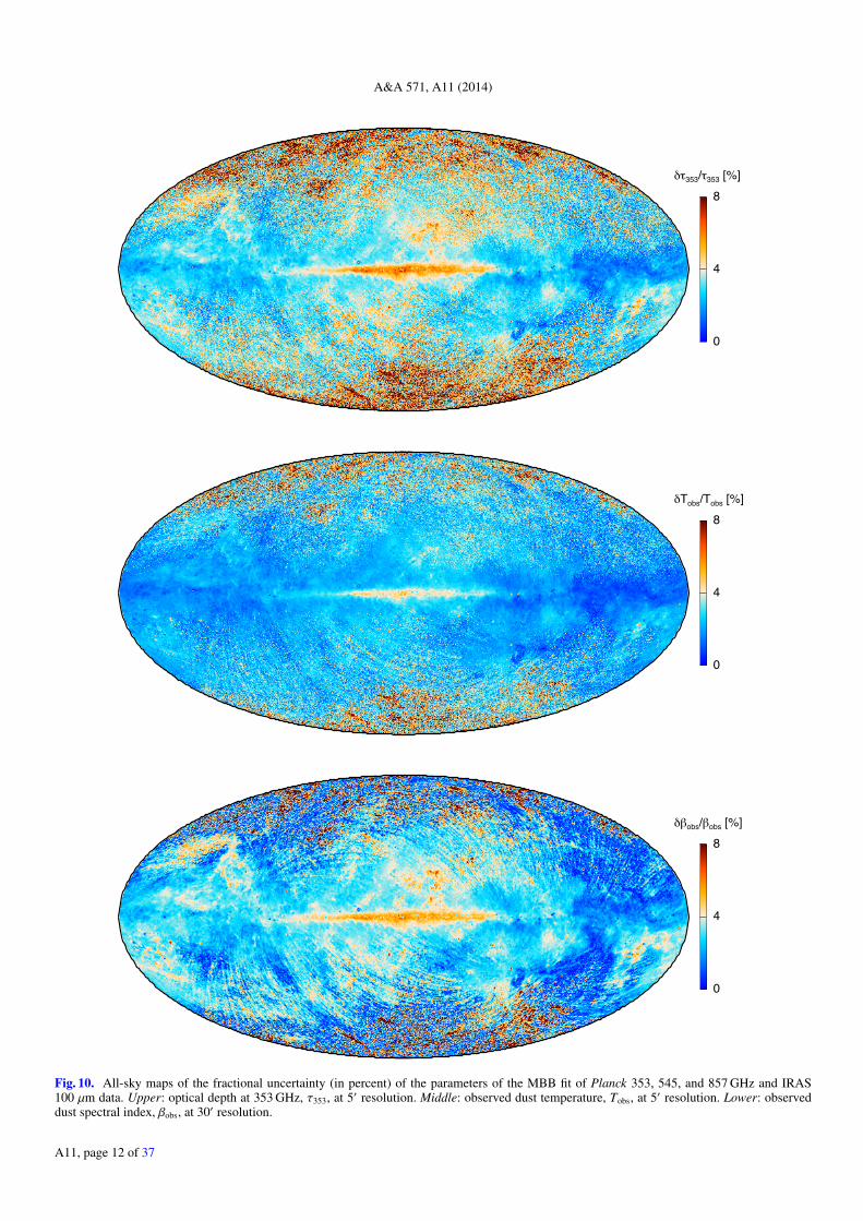
The three uncertainty maps have a similar spatial structure.In general the fractional uncertainties are higher in the most dif-fuse areas of the sky (where the noise and the CIBA have a moreimportant contribution) and in the inner Galaxy region. Stripingpatterns are visible, especially in the Tobs uncertainty map; theseare likely to be coming from the IRAS data. The uncertainty ofTobs is of the order of 1–3% in bright areas, with a noticeable in-crease in the inner Galaxy and rising to 5–8% in the most diffuseareas of the sky. The same general trend is seen for τ353 but withhigher values: 2–5% in bright areas and up to 10% in diffuse ar-eas. The uncertainty of βobs, based on analysis at 30′ resolution,has a slightly different spatial structure. It is typically of 3–4%with a smaller decrease in bright areas and a noticeable increasein the inner Galaxy to 6–8%.

The reduced χ2 of the fit is much smaller than unity overmost of the sky, due to the fact that calibration uncertainties aretaken into account in the fit to give less weight to data points withless precise calibration (Appendix B). To illustrate this, Fig. 11shows the distribution function of (Data−Model)/Noise for eachfrequency used in the fit. The noise used here follows the defini-tion of Eq. (B.1); it takes into account instrumental noise and theuncertainties of the calibration, the zero level, and the CMB sub-traction. The range adopted in Fig. 11 corresponds to only ±1σ.At 353 and 3000 GHz, for most of the sky pixels the data are fit-ted more tightly (to better than 0.1σ) than at 545 and 857 GHz.This implies that 353 and 3000 GHz have a lot of weight inthe estimation of the parameters. The 3000 GHz band providesthe only data point on the Wien part of the MBB and thereforestrongly influences the determination of Tobs. On the other hand,the 353 GHz band strongly influences the determination of τ353and βobs because it is the closest to the Rayleigh-Jeans part of thespectrum. The compensating small offsets of the distributions at

A11, page 10 of 37

Planck collaboration: Planck 2013 results. XI.

-6

-5

-4

-3log10(o353)

15

19

23

27Tobs [K]

1.2

1.4

1.6

1.8

2.0

2.2`obs

Fig. 9. All-sky maps of the parameters of the MBB fit of Planck 353, 545, and 857 GHz and IRAS 100 µm data. Upper: optical depth at 353 GHz,τ353, at 5′ resolution, displayed logarithmically (the range shown corresponds to −6.5 < log10(τ353) < −3). Middle: observed dust temperature,Tobs, at 5′ resolution, in kelvin. Lower: observed dust spectral index, βobs, at 30′ resolution.

A11, page 11 of 37

A&A 571, A11 (2014)

0

4

8bo353/o353 [%]

0

4

8bTobs/Tobs [%]

0

4

8b`obs/`obs [%]

Fig. 10. All-sky maps of the fractional uncertainty (in percent) of the parameters of the MBB fit of Planck 353, 545, and 857 GHz and IRAS100 µm data. Upper: optical depth at 353 GHz, τ353, at 5′ resolution. Middle: observed dust temperature, Tobs, at 5′ resolution. Lower: observeddust spectral index, βobs, at 30′ resolution.

A11, page 12 of 37

Planck collaboration: Planck 2013 results. XI.

-1.0 -0.5 0.0 0.5 1.0(Data-Model)/Noise

0.0

0.2

0.4

0.6

0.8

1.0

ND

F

353 GHz545 GHz857 GHz

3000 GHz

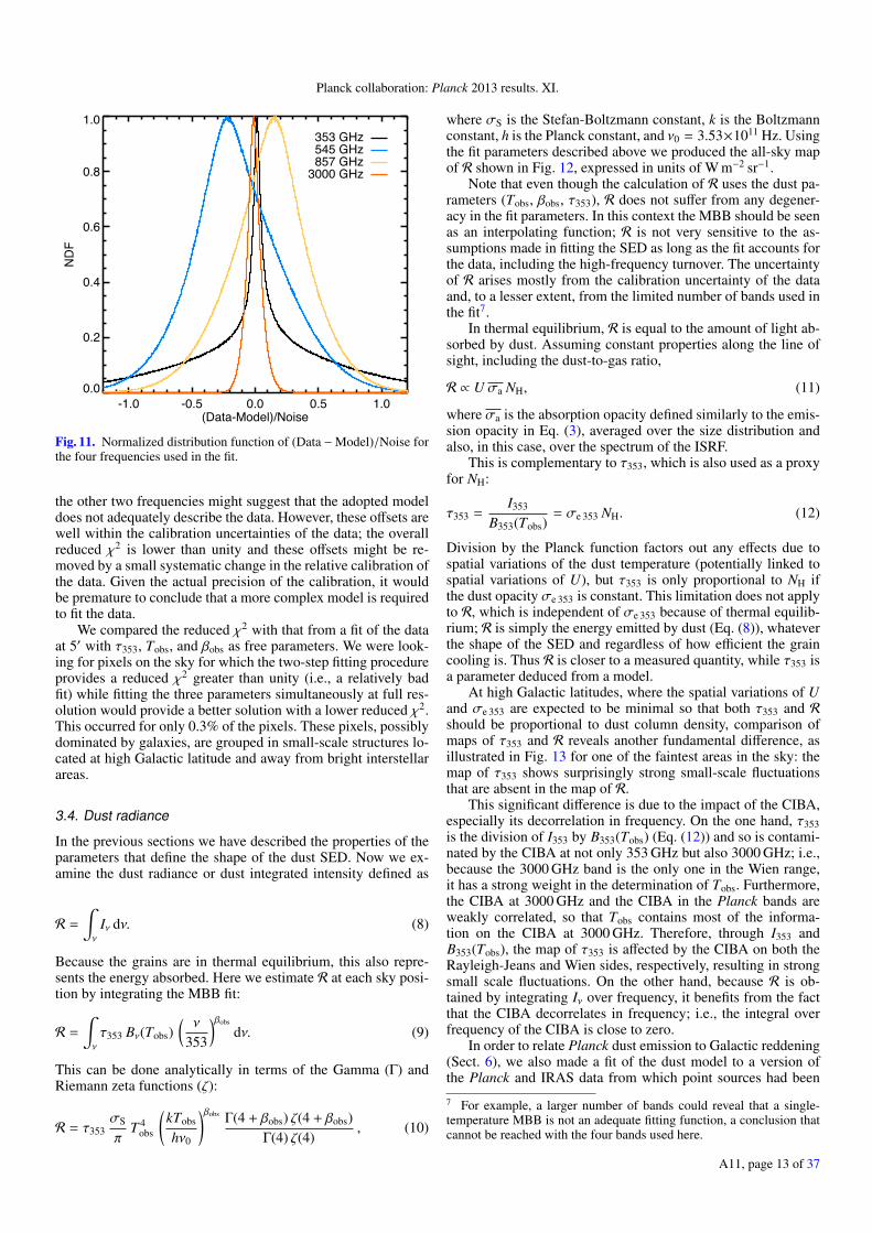
Fig. 11. Normalized distribution function of (Data −Model)/Noise forthe four frequencies used in the fit.

the other two frequencies might suggest that the adopted modeldoes not adequately describe the data. However, these offsets arewell within the calibration uncertainties of the data; the overallreduced χ2 is lower than unity and these offsets might be re-moved by a small systematic change in the relative calibration ofthe data. Given the actual precision of the calibration, it wouldbe premature to conclude that a more complex model is requiredto fit the data.

We compared the reduced χ2 with that from a fit of the dataat 5′ with τ353, Tobs, and βobs as free parameters. We were look-ing for pixels on the sky for which the two-step fitting procedureprovides a reduced χ2 greater than unity (i.e., a relatively badfit) while fitting the three parameters simultaneously at full res-olution would provide a better solution with a lower reduced χ2.This occurred for only 0.3% of the pixels. These pixels, possiblydominated by galaxies, are grouped in small-scale structures lo-cated at high Galactic latitude and away from bright interstellarareas.

3.4. Dust radiance

In the previous sections we have described the properties of theparameters that define the shape of the dust SED. Now we ex-amine the dust radiance or dust integrated intensity defined as

R =

∫ν

Iν dν. (8)

Because the grains are in thermal equilibrium, this also repre-sents the energy absorbed. Here we estimate R at each sky posi-tion by integrating the MBB fit:

R =

∫ν

τ353 Bν(Tobs)(ν

353

)βobs

dν. (9)

This can be done analytically in terms of the Gamma (Γ) andRiemann zeta functions (ζ):

R = τ353σS

πT 4

obs

(kTobs

hν0

)βobs Γ(4 + βobs) ζ(4 + βobs)Γ(4) ζ(4)

, (10)

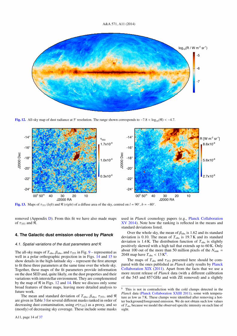
where σS is the Stefan-Boltzmann constant, k is the Boltzmannconstant, h is the Planck constant, and ν0 = 3.53×1011 Hz. Usingthe fit parameters described above we produced the all-sky mapof R shown in Fig. 12, expressed in units of W m−2 sr−1.

Note that even though the calculation of R uses the dust pa-rameters (Tobs, βobs, τ353), R does not suffer from any degener-acy in the fit parameters. In this context the MBB should be seenas an interpolating function; R is not very sensitive to the as-sumptions made in fitting the SED as long as the fit accounts forthe data, including the high-frequency turnover. The uncertaintyof R arises mostly from the calibration uncertainty of the dataand, to a lesser extent, from the limited number of bands used inthe fit7.

In thermal equilibrium, R is equal to the amount of light ab-sorbed by dust. Assuming constant properties along the line ofsight, including the dust-to-gas ratio,

R ∝ U σa NH, (11)

where σa is the absorption opacity defined similarly to the emis-sion opacity in Eq. (3), averaged over the size distribution andalso, in this case, over the spectrum of the ISRF.

This is complementary to τ353, which is also used as a proxyfor NH:

τ353 =I353

B353(Tobs)= σe 353 NH. (12)

Division by the Planck function factors out any effects due tospatial variations of the dust temperature (potentially linked tospatial variations of U), but τ353 is only proportional to NH ifthe dust opacity σe 353 is constant. This limitation does not applyto R, which is independent of σe 353 because of thermal equilib-rium; R is simply the energy emitted by dust (Eq. (8)), whateverthe shape of the SED and regardless of how efficient the graincooling is. Thus R is closer to a measured quantity, while τ353 isa parameter deduced from a model.

At high Galactic latitudes, where the spatial variations of Uand σe 353 are expected to be minimal so that both τ353 and Rshould be proportional to dust column density, comparison ofmaps of τ353 and R reveals another fundamental difference, asillustrated in Fig. 13 for one of the faintest areas in the sky: themap of τ353 shows surprisingly strong small-scale fluctuationsthat are absent in the map of R.

This significant difference is due to the impact of the CIBA,especially its decorrelation in frequency. On the one hand, τ353is the division of I353 by B353(Tobs) (Eq. (12)) and so is contami-nated by the CIBA at not only 353 GHz but also 3000 GHz; i.e.,because the 3000 GHz band is the only one in the Wien range,it has a strong weight in the determination of Tobs. Furthermore,the CIBA at 3000 GHz and the CIBA in the Planck bands areweakly correlated, so that Tobs contains most of the informa-tion on the CIBA at 3000 GHz. Therefore, through I353 andB353(Tobs), the map of τ353 is affected by the CIBA on both theRayleigh-Jeans and Wien sides, respectively, resulting in strongsmall scale fluctuations. On the other hand, because R is ob-tained by integrating Iν over frequency, it benefits from the factthat the CIBA decorrelates in frequency; i.e., the integral overfrequency of the CIBA is close to zero.

In order to relate Planck dust emission to Galactic reddening(Sect. 6), we also made a fit of the dust model to a version ofthe Planck and IRAS data from which point sources had been

7 For example, a larger number of bands could reveal that a single-temperature MBB is not an adequate fitting function, a conclusion thatcannot be reached with the four bands used here.

A11, page 13 of 37

A&A 571, A11 (2014)

-7

-6

-5

log10(R / W m-2 sr-1)

Fig. 12. All-sky map of dust radiance at 5′ resolution. The range shown corresponds to −7.8 < log10(R) < −4.7.

00h 50m 40 30 20 10 J2000 RA

-24°

-22°

-20°

-18°

-16°

-14°

J200

0 D

ec

0.3x10-6

1.0x10-6

1.7x10-6

o353

00h 50m 40 30 20 10 J2000 RA

-24°

-22°

-20°

-18°

-16°

-14°

J200

0 D

ec

2.7x10-8

5.6x10-8

8.6x10-8

R [W m-2 sr-1]

Fig. 13. Maps of τ353 (left) and R (right) of a diffuse area of the sky, centred on l = 90◦, b = −80◦.

removed (Appendix D). From this fit we have also made mapsof τ353 and R.

4. The Galactic dust emission observed by Planck

4.1. Spatial variations of the dust parameters and R

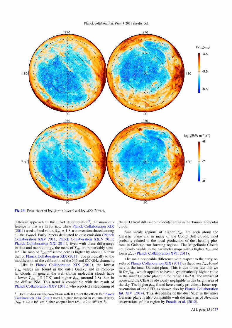
The all-sky maps of Tobs, βobs, and τ353 in Fig. 9 – represented aswell in a polar orthographic projection in in Figs. 14 and 15 toshow details in the high-latitude sky – represent the first attemptto fit these three parameters at the same time over the whole sky.Together, these maps of the fit parameters provide informationon the dust SED and, quite likely, on the dust properties and theirvariations with interstellar environment. They are complementedby the map of R in Figs. 12 and 14. Here we discuss only somebroad features of these maps, leaving more detailed analysis tofuture work.

The mean and standard deviation of Tobs, βobs, τ353, and Rare given in Table 3 for several different masks ranked in order ofdecreasing dust contamination, using σ(τ353) as a proxy, and so(mostly) of decreasing sky coverage. These include some masks

used in Planck cosmology papers (e.g., Planck CollaborationXV 2014). Note how the ranking is reflected in the means andstandard deviations listed.

Over the whole sky, the mean of βobs is 1.62 and its standarddeviation is 0.10. The mean of Tobs is 19.7 K and its standarddeviation is 1.4 K. The distribution function of Tobs is slightlypositively skewed with a high tail that extends up to 60 K. Onlyabout 100 out of the more than 50 million pixels of the Nside =2048 map have Tobs < 13 K8.

The maps of Tobs and τ353 presented here should be com-pared with the ones published as Planck early results by PlanckCollaboration XIX (2011). Apart from the facts that we use amore recent release of Planck data (with a different calibrationof the 545 and 857 GHz and with ZE removed) and a slightly

8 This is not in contradiction with the cold clumps detected in thePlanck data (Planck Collaboration XXIII 2011), some with tempera-ture as low as 7 K. These clumps were identified after removing a hot-ter background/foreground emission. We do not obtain such low valuesof Tobs because we model the observed specific intensity on each line ofsight.

A11, page 14 of 37

Planck collaboration: Planck 2013 results. XI.

-6.5

-5.5

-4.5

90

180

270

90

180

270

log10(o353)

-8

-7

-6

90

180

270

90

180

270

log10(R/W m-2 sr-1)

Fig. 14. Polar views of log10(τ353) (upper) and log10(R) (lower).

different approach to the offset determination9, the main dif-ference is that we fit for βobs while Planck Collaboration XIX(2011) used a fixed value, βobs = 1.8, a convention shared amongall the Planck Early Papers dedicated to dust emission (PlanckCollaboration XXV 2011; Planck Collaboration XXIV 2011;Planck Collaboration XXI 2011). Even with these differencesin data and methodology, the maps of Tobs are remarkably simi-lar. The map of Tobs presented here is higher by about 1 K thanthat of Planck Collaboration XIX (2011), due principally to themodification of the calibration of the 545 and 857 GHz channels.

Like in Planck Collaboration XIX (2011), the lowestTobs values are found in the outer Galaxy and in molecu-lar clouds. In general the well-known molecular clouds havea lower Tobs (15–17 K) and higher βobs (around 1.8) than inthe diffuse ISM. This trend is compatible with the result ofPlanck Collaboration XXV (2011) who reported a steepening of

9 Both studies use the correlation with H to set the offsets but PlanckCollaboration XIX (2011) used a higher threshold in column density(NH < 1.2 × 1021 cm−2) than adopted here (NH < 2 × 1020 cm−2).

the SED from diffuse to molecular areas in the Taurus molecularcloud.

Small-scale regions of higher Tobs are seen along theGalactic plane and in many of the Gould Belt clouds, mostprobably related to the local production of dust-heating pho-tons in Galactic star forming regions. The Magellanic Cloudsare clearly visible in the parameter maps with a higher Tobs andlower βobs (Planck Collaboration XVII 2011).

The main noticeable difference with respect to the early re-sults of Planck Collaboration XIX (2011) is the lower Tobs foundhere in the inner Galactic plane. This is due to the fact that wefit for βobs, which appears to have a systematically higher valuein the inner Galactic plane, in the range 1.8–2.0. The impact ofnoise and the CIBA is obviously negligible in this bright area ofthe sky. The higher βobs found here clearly provides a better rep-resentation of the SED, as shown also by Planck CollaborationInt. XIV (2014). This steepening of the dust SED in the innerGalactic plane is also compatible with the analysis of Herschelobservations of that region by Paradis et al. (2012).

A11, page 15 of 37

A&A 571, A11 (2014)

15

19

23

27

90

180

270

90

180

270

Tobs [K]

1.2

1.4

1.6

1.8

2.0

90

180

270

90

180

270

`obs

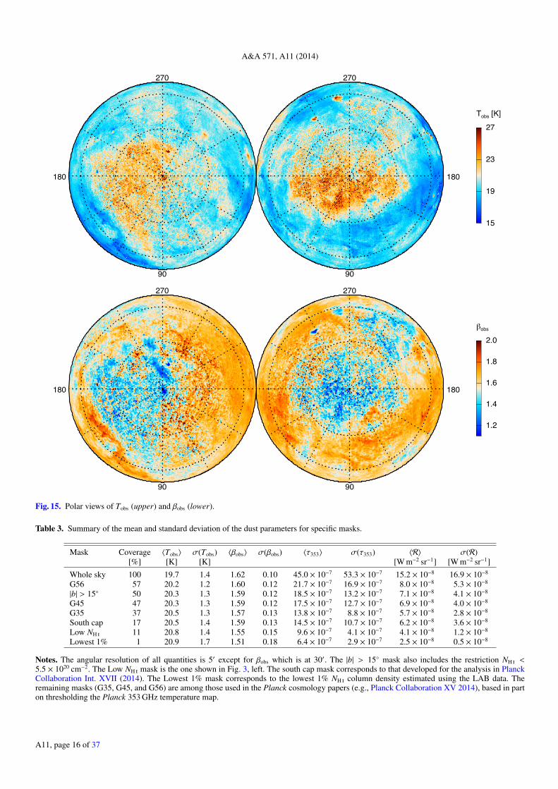
Fig. 15. Polar views of Tobs (upper) and βobs (lower).

Table 3. Summary of the mean and standard deviation of the dust parameters for specific masks.

Mask Coverage 〈Tobs〉 σ(Tobs) 〈βobs〉 σ(βobs) 〈τ353〉 σ(τ353) 〈R〉 σ(R)[%] [K] [K] [W m−2 sr−1] [W m−2 sr−1]

Whole sky 100 19.7 1.4 1.62 0.10 45.0 × 10−7 53.3 × 10−7 15.2 × 10−8 16.9 × 10−8

G56 57 20.2 1.2 1.60 0.12 21.7 × 10−7 16.9 × 10−7 8.0 × 10−8 5.3 × 10−8

|b| > 15◦ 50 20.3 1.3 1.59 0.12 18.5 × 10−7 13.2 × 10−7 7.1 × 10−8 4.1 × 10−8

G45 47 20.3 1.3 1.59 0.12 17.5 × 10−7 12.7 × 10−7 6.9 × 10−8 4.0 × 10−8

G35 37 20.5 1.3 1.57 0.13 13.8 × 10−7 8.8 × 10−7 5.7 × 10−8 2.8 × 10−8

South cap 17 20.5 1.4 1.59 0.13 14.5 × 10−7 10.7 × 10−7 6.2 × 10−8 3.6 × 10−8

Low NH 11 20.8 1.4 1.55 0.15 9.6 × 10−7 4.1 × 10−7 4.1 × 10−8 1.2 × 10−8

Lowest 1% 1 20.9 1.7 1.51 0.18 6.4 × 10−7 2.9 × 10−7 2.5 × 10−8 0.5 × 10−8

Notes. The angular resolution of all quantities is 5′ except for βobs which is at 30′. The |b| > 15◦ mask also includes the restriction NH <5.5 × 1020 cm−2. The Low NH mask is the one shown in Fig. 3, left. The south cap mask corresponds to that developed for the analysis in PlanckCollaboration Int. XVII (2014). The Lowest 1% mask corresponds to the lowest 1% NH column density estimated using the LAB data. Theremaining masks (G35, G45, and G56) are among those used in the Planck cosmology papers (e.g., Planck Collaboration XV 2014), based in parton thresholding the Planck 353 GHz temperature map.

A11, page 16 of 37

Planck collaboration: Planck 2013 results. XI.

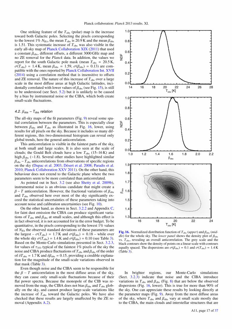
One striking feature of the Tobs (polar) map is the increasetoward both Galactic poles. Selecting the pixels correspondingto the lowest 1% NH , the mean Tobs is 20.9 K and the mean βobsis 1.51. This systematic increase of Tobs was also visible in theearly all-sky map of Planck Collaboration XIX (2011) that useda constant βobs, different offsets, a different 3000 GHz map andno ZE removal for the Planck data. In addition, the values wereport for the south Galactic pole mask (mean Tobs = 20.5 K,σ(Tobs) = 1.4 K, mean βobs = 1.59, σ(βobs) = 0.13) are com-patible with the ones reported by Planck Collaboration Int. XVII(2014) using a correlation method that is insensitive to offsetsand ZE removal. The nature of this increase of Tobs over a largescale in the most diffuse areas at high Galactic latitudes, inci-dentally correlated with lower values of βobs (see Fig. 15), is stillto be understood (see Sect. 5.2) but it is unlikely to be causedby a bias by instrumental noise or the CIBA, which both createsmall-scale fluctuations.

4.2. βobs – Tobs relation

The all-sky maps of the fit parameters (Fig. 9) reveal some spa-tial correlation between the parameters. This is especially clearbetween βobs and Tobs as illustrated in Fig. 16, lower, usingresults for all pixels on the sky. Because it includes so many dif-ferent regions, this two-dimensional histogram can reveal onlyglobal trends, here the general anticorrelation.

This anticorrelation is visible in the faintest parts of the sky,at both small and large scales. It is also seen at the scale ofclouds; the Gould Belt clouds have a low Tobs (15–16 K) andhigh βobs (∼1.8). Several other studies have highlighted similarβobs − Tobs anticorrelations from observations of specific regionson the sky (Dupac et al. 2003; Désert et al. 2008; Paradis et al.2010; Planck Collaboration XXV 2011). On the other hand, thisbehaviour does not extend to the Galactic plane where the twoparameters seem to be more correlated than anticorrelated.

As pointed out in Sect. 3.2 (see also Shetty et al. 2009b),instrumental noise is an obvious candidate that might create aβ − T anticorrelation. However, the fractional variations of βobsand Tobs observed here over most of the sky significantly ex-ceed the statistical uncertainties of these parameters taking intoaccount noise and calibration uncertainties (see Fig. 10).

On the other hand, as shown in Sect. 3.2.2 and Appendix C,for faint dust emission the CIBA can produce significant varia-tions of Tobs and βobs at small scales, and although this effect isin fact observed, it is not accounted for in the error budget. To bequantitative, in the pixels corresponding to the lowest 1% valuesof NH the observed standard deviations of these parameters arethe largest – σ(Tobs) = 1.7 K and σ(βobs) = 0.18 – while overthe whole sky σ(Tobs) = 1.4 K and σ(βobs) = 0.10 (see Table 3).Based on the Monte-Carlo simulations presented in Sect. 3.2.3,for values of τ353 typical of the faintest 1% pixels of the sky thenoise and CIBA produce fluctuations of Tobs and βobs of the orderof δTobs = 1.7 K and δβobs = 0.15, providing a credible explana-tion for the magnitude of the small-scale variations observed inthat mask (Table 3).

Even though noise and the CIBA seem to be responsible forthe β − T anticorrelation in the most diffuse areas of the sky,they can cause only small-scale fluctuations because of theirflat power spectra. Because the monopole of the CIB was re-moved from the map, the CIBA does not bias βobs and Tobs glob-ally on the sky, and cannot produce large-scale variations likethe increase of Tobs toward the Galactic poles. We have alsochecked that these results are largely unaffected by the ZE re-moval (Appendix A.2).

14 16 18 20 22 24 26 28Tobs [K]

0.0

0.2

0.4

0.6

0.8

1.0

ND

F

1.0 1.2 1.4 1.6 1.8 2.0 2.2`obs

0.0

0.2

0.4

0.6

0.8

1.0

NDF

16 18 20 22 24Tobs [K]

1.3

1.4

1.5

1.6

1.7

1.8

1.9

` obs

Fig. 16. Normalized distribution function of Tobs (upper) and βobs (mid-dle) for the whole sky. The lower panel shows the density plot of βobsvs. Tobs, revealing an overall anticorrelation. The grey scale and theblack contours show the density of points on a linear scale with contoursequally spaced. The dispersions are σ(βobs) = 0.1 and σ(Tobs) = 1.4 K(Table 3).

In brighter regions, our Monte-Carlo simulations(Sect. 3.2.3) indicate that noise and the CIBA introducevariations in Tobs and βobs (Fig. 8) that are below the observeddispersions (Fig. 16, lower). This is true for more than 90% ofthe sky. One can appreciate these results by looking directly atthe parameter maps (Fig. 9). Away from the most diffuse areasof the sky, where Tobs and βobs vary at small scale mostly dueto the CIBA, the main clouds and interstellar structures that are

A11, page 17 of 37

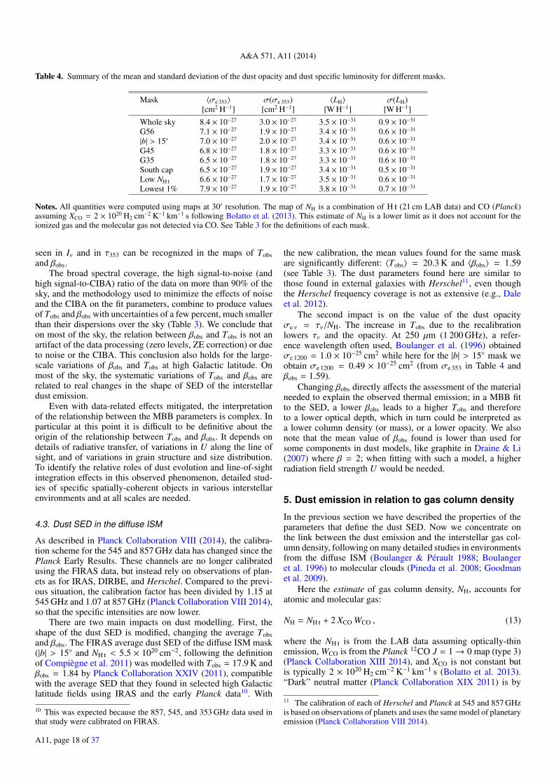
A&A 571, A11 (2014)

Table 4. Summary of the mean and standard deviation of the dust opacity and dust specific luminosity for different masks.

Mask 〈σe 353〉 σ(σe 353) 〈LH〉 σ(LH)[cm2 H−1] [cm2 H−1] [W H−1] [W H−1]

Whole sky 8.4 × 10−27 3.0 × 10−27 3.5 × 10−31 0.9 × 10−31

G56 7.1 × 10−27 1.9 × 10−27 3.4 × 10−31 0.6 × 10−31

|b| > 15◦ 7.0 × 10−27 2.0 × 10−27 3.4 × 10−31 0.6 × 10−31

G45 6.8 × 10−27 1.8 × 10−27 3.3 × 10−31 0.6 × 10−31

G35 6.5 × 10−27 1.8 × 10−27 3.3 × 10−31 0.6 × 10−31

South cap 6.5 × 10−27 1.9 × 10−27 3.4 × 10−31 0.5 × 10−31

Low NH 6.6 × 10−27 1.7 × 10−27 3.5 × 10−31 0.6 × 10−31

Lowest 1% 7.9 × 10−27 1.9 × 10−27 3.8 × 10−31 0.7 × 10−31

Notes. All quantities were computed using maps at 30′ resolution. The map of NH is a combination of H (21 cm LAB data) and CO (Planck)assuming XCO = 2 × 1020 H2 cm−2 K−1 km−1 s following Bolatto et al. (2013). This estimate of NH is a lower limit as it does not account for theionized gas and the molecular gas not detected via CO. See Table 3 for the definitions of each mask.

seen in Iν and in τ353 can be recognized in the maps of Tobsand βobs.

The broad spectral coverage, the high signal-to-noise (andhigh signal-to-CIBA) ratio of the data on more than 90% of thesky, and the methodology used to minimize the effects of noiseand the CIBA on the fit parameters, combine to produce valuesof Tobs and βobs with uncertainties of a few percent, much smallerthan their dispersions over the sky (Table 3). We conclude thaton most of the sky, the relation between βobs and Tobs is not anartifact of the data processing (zero levels, ZE correction) or dueto noise or the CIBA. This conclusion also holds for the large-scale variations of βobs and Tobs at high Galactic latitude. Onmost of the sky, the systematic variations of Tobs and βobs arerelated to real changes in the shape of SED of the interstellardust emission.

Even with data-related effects mitigated, the interpretationof the relationship between the MBB parameters is complex. Inparticular at this point it is difficult to be definitive about theorigin of the relationship between Tobs and βobs. It depends ondetails of radiative transfer, of variations in U along the line ofsight, and of variations in grain structure and size distribution.To identify the relative roles of dust evolution and line-of-sightintegration effects in this observed phenomenon, detailed stud-ies of specific spatially-coherent objects in various interstellarenvironments and at all scales are needed.

4.3. Dust SED in the diffuse ISM

As described in Planck Collaboration VIII (2014), the calibra-tion scheme for the 545 and 857 GHz data has changed since thePlanck Early Results. These channels are no longer calibratedusing the FIRAS data, but instead rely on observations of plan-ets as for IRAS, DIRBE, and Herschel. Compared to the previ-ous situation, the calibration factor has been divided by 1.15 at545 GHz and 1.07 at 857 GHz (Planck Collaboration VIII 2014),so that the specific intensities are now lower.

There are two main impacts on dust modelling. First, theshape of the dust SED is modified, changing the average Tobsand βobs. The FIRAS average dust SED of the diffuse ISM mask(|b| > 15◦ and NH < 5.5 × 1020 cm−2, following the definitionof Compiègne et al. 2011) was modelled with Tobs = 17.9 K andβobs = 1.84 by Planck Collaboration XXIV (2011), compatiblewith the average SED that they found in selected high Galacticlatitude fields using IRAS and the early Planck data10. With

10 This was expected because the 857, 545, and 353 GHz data used inthat study were calibrated on FIRAS.

the new calibration, the mean values found for the same maskare significantly different: 〈Tobs〉 = 20.3 K and 〈βobs〉 = 1.59(see Table 3). The dust parameters found here are similar tothose found in external galaxies with Herschel11, even thoughthe Herschel frequency coverage is not as extensive (e.g., Daleet al. 2012).

The second impact is on the value of the dust opacityσe ν = τν/NH. The increase in Tobs due to the recalibrationlowers τν and the opacity. At 250 µm (1 200 GHz), a refer-ence wavelength often used, Boulanger et al. (1996) obtainedσe 1200 = 1.0 × 10−25 cm2 while here for the |b| > 15◦ mask weobtain σe 1200 = 0.49 × 10−25 cm2 (from σe 353 in Table 4 andβobs = 1.59).

Changing βobs directly affects the assessment of the materialneeded to explain the observed thermal emission; in a MBB fitto the SED, a lower βobs leads to a higher Tobs and thereforeto a lower optical depth, which in turn could be interpreted asa lower column density (or mass), or a lower opacity. We alsonote that the mean value of βobs found is lower than used forsome components in dust models, like graphite in Draine & Li(2007) where β = 2; when fitting with such a model, a higherradiation field strength U would be needed.

5. Dust emission in relation to gas column density

In the previous section we have described the properties of theparameters that define the dust SED. Now we concentrate onthe link between the dust emission and the interstellar gas col-umn density, following on many detailed studies in environmentsfrom the diffuse ISM (Boulanger & Pérault 1988; Boulangeret al. 1996) to molecular clouds (Pineda et al. 2008; Goodmanet al. 2009).

Here the estimate of gas column density, NH, accounts foratomic and molecular gas:

NH = NH + 2 XCO WCO , (13)

where the NH is from the LAB data assuming optically-thinemission, WCO is from the Planck 12CO J = 1→ 0 map (type 3)(Planck Collaboration XIII 2014), and XCO is not constant butis typically 2 × 1020 H2 cm−2 K−1 km−1 s (Bolatto et al. 2013).“Dark” neutral matter (Planck Collaboration XIX 2011) is by

11 The calibration of each of Herschel and Planck at 545 and 857 GHzis based on observations of planets and uses the same model of planetaryemission (Planck Collaboration VIII 2014).

A11, page 18 of 37

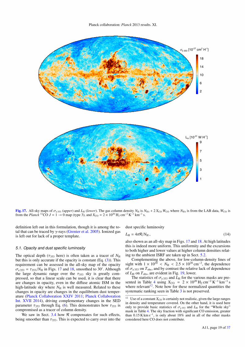
Planck collaboration: Planck 2013 results. XI.

2

6

10

14

18

me 353 [10-27 cm2 H-1]

1

3

5

7

9LH [10-31 W H-1]

Fig. 17. All-sky maps of σe 353 (upper) and LH (lower). The gas column density NH is NH + 2 XCO WCO where NH is from the LAB data, WCO isfrom the Planck 12CO J = 1→ 0 map (type 3), and XCO = 2 × 1020 H2 cm−2 K−1 km−1 s.

definition left out in this formulation, though it is among the to-tal that can be traced by γ-rays (Grenier et al. 2005). Ionized gasis left out for lack of a proper template.

5.1. Opacity and dust specific luminosity

The optical depth (τ353 here) is often taken as a tracer of NHbut this is only accurate if the opacity is constant (Eq. (3)). Thisrequirement can be assessed in the all-sky map of the opacityσe 353 = τ353/NH in Figs. 17 and 18, smoothed to 30′. Althoughthe large dynamic range over the τ353 sky is greatly com-pressed, so that a linear scale can be used, it is clear that thereare changes in opacity, even in the diffuse atomic ISM in thehigh-latitude sky where NH is well measured. Related to thesechanges in opacity are changes in the equilibrium dust temper-ature (Planck Collaboration XXIV 2011; Planck CollaborationInt. XVII 2014), driving complementary changes in the SEDparameter τ353 through Eq. (6). This demonstrates how τ353 iscompromised as a tracer of column density.

We saw in Sect. 3.4 how R compensates for such effects,being smoother than τ353. This is expected to carry over into the

dust specific luminosity

LH = 4πR/NH , (14)

also shown as an all-sky map in Figs. 17 and 18. At high latitudesthis is indeed more uniform. This uniformity and the excursionsto both higher and lower values at higher column densities relat-ing to the ambient ISRF are taken up in Sect. 5.2.

Complementing the above, for low-column-density lines ofsight with 1 × 1020 < NH < 2.5 × 1020 cm−2, the dependenceof σe 353 on Tobs, and by contrast the relative lack of dependenceof LH on Tobs, are evident in Fig. 19, lower.

The statistics of σe 353 and LH for the various masks are pre-sented in Table 4 using XCO = 2 × 1020 H2 cm−2 K−1 km−1 swhere relevant12. Note how for these normalized quantities thesystematic ranking seen in Table 3 is not preserved.

12 Use of a constant XCO is certainly not realistic, given the large rangesin density and temperature covered. On the other hand, it is used hereonly to provide basic statistics of σe 353 and LH for the “Whole sky”mask in Table 4. The sky fraction with significant CO emission, greaterthan 0.15 K km s−1, is only about 18% and in all of the other masksconsidered here CO does not contribute.

A11, page 19 of 37

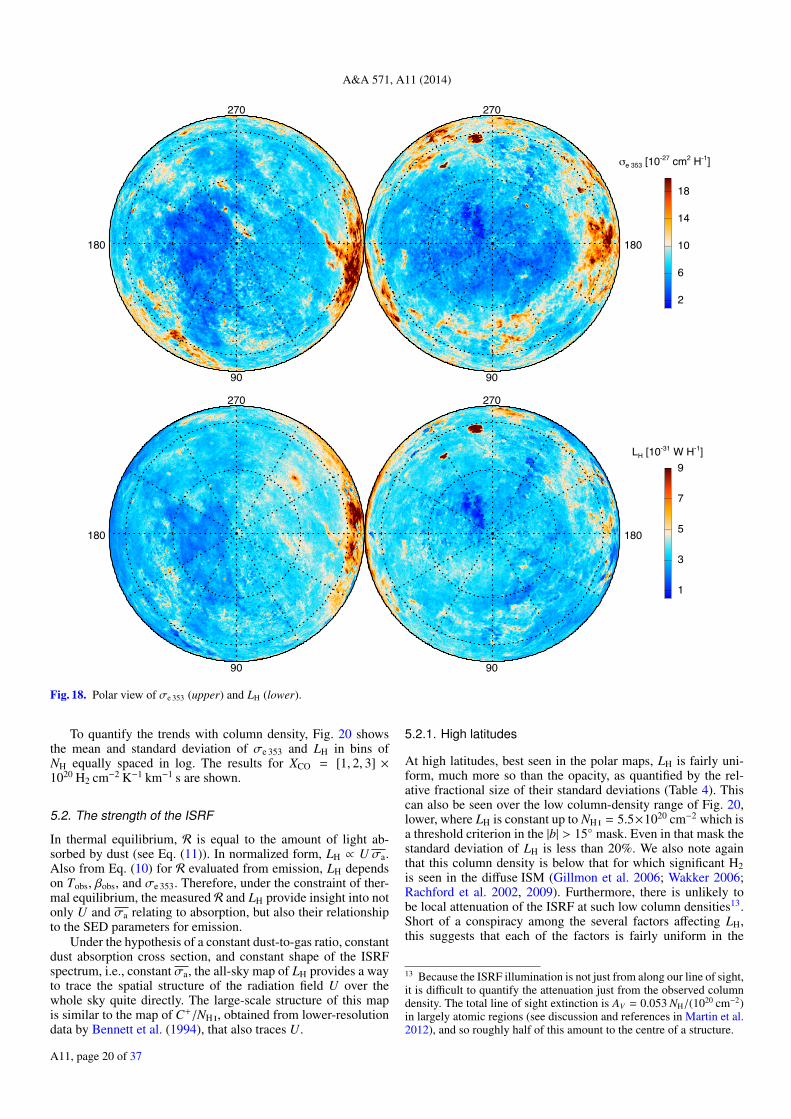
A&A 571, A11 (2014)

2

6

10

14

18

90

180

270

90

180

270

me 353 [10-27 cm2 H-1]

1

3

5

7

9

90

180

270

90

180

270

LH [10-31 W H-1]

Fig. 18. Polar view of σe 353 (upper) and LH (lower).

To quantify the trends with column density, Fig. 20 showsthe mean and standard deviation of σe 353 and LH in bins ofNH equally spaced in log. The results for XCO = [1, 2, 3] ×1020 H2 cm−2 K−1 km−1 s are shown.

5.2. The strength of the ISRF

In thermal equilibrium, R is equal to the amount of light ab-sorbed by dust (see Eq. (11)). In normalized form, LH ∝ U σa.Also from Eq. (10) for R evaluated from emission, LH dependson Tobs, βobs, and σe 353. Therefore, under the constraint of ther-mal equilibrium, the measured R and LH provide insight into notonly U and σa relating to absorption, but also their relationshipto the SED parameters for emission.

Under the hypothesis of a constant dust-to-gas ratio, constantdust absorption cross section, and constant shape of the ISRFspectrum, i.e., constant σa, the all-sky map of LH provides a wayto trace the spatial structure of the radiation field U over thewhole sky quite directly. The large-scale structure of this mapis similar to the map of C+/NH , obtained from lower-resolutiondata by Bennett et al. (1994), that also traces U.

5.2.1. High latitudes

At high latitudes, best seen in the polar maps, LH is fairly uni-form, much more so than the opacity, as quantified by the rel-ative fractional size of their standard deviations (Table 4). Thiscan also be seen over the low column-density range of Fig. 20,lower, where LH is constant up to NH = 5.5×1020 cm−2 which isa threshold criterion in the |b| > 15◦ mask. Even in that mask thestandard deviation of LH is less than 20%. We also note againthat this column density is below that for which significant H2is seen in the diffuse ISM (Gillmon et al. 2006; Wakker 2006;Rachford et al. 2002, 2009). Furthermore, there is unlikely tobe local attenuation of the ISRF at such low column densities13.Short of a conspiracy among the several factors affecting LH,this suggests that each of the factors is fairly uniform in the

13 Because the ISRF illumination is not just from along our line of sight,it is difficult to quantify the attenuation just from the observed columndensity. The total line of sight extinction is AV = 0.053 NH/(1020 cm−2)in largely atomic regions (see discussion and references in Martin et al.2012), and so roughly half of this amount to the centre of a structure.

A11, page 20 of 37

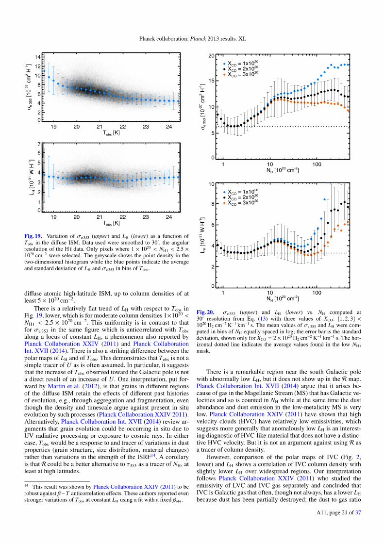
Planck collaboration: Planck 2013 results. XI.

19 20 21 22 23 24Tobs [K]

02468

101214

me

353 [

10-2

7 cm

2 H-1]

19 20 21 22 23 24Tobs [K]

01

2

3

4

5

67

L H [1

0-31 W

H-1]

Fig. 19. Variation of σe 353 (upper) and LH (lower) as a function ofTobs in the diffuse ISM. Data used were smoothed to 30′, the angularresolution of the H data. Only pixels where 1 × 1020 < NH < 2.5 ×1020 cm−2 were selected. The greyscale shows the point density in thetwo-dimensional histogram while the blue points indicate the averageand standard deviation of LH and σe 353 in bins of Tobs.

diffuse atomic high-latitude ISM, up to column densities of atleast 5 × 1020 cm−2.

There is a relatively flat trend of LH with respect to Tobs inFig. 19, lower, which is for moderate column densities 1×1020 <NH < 2.5 × 1020 cm−2. This uniformity is in contrast to thatfor σe 353 in the same figure which is anticorrelated with Tobsalong a locus of constant LH, a phenomenon also reported byPlanck Collaboration XXIV (2011) and Planck CollaborationInt. XVII (2014). There is also a striking difference between thepolar maps of LH and of Tobs. This demonstrates that Tobs is not asimple tracer of U as is often assumed. In particular, it suggeststhat the increase of Tobs observed toward the Galactic pole is nota direct result of an increase of U. One interpretation, put for-ward by Martin et al. (2012), is that grains in different regionsof the diffuse ISM retain the effects of different past historiesof evolution, e.g., through aggregation and fragmentation, eventhough the density and timescale argue against present in situevolution by such processes (Planck Collaboration XXIV 2011).Alternatively, Planck Collaboration Int. XVII (2014) review ar-guments that grain evolution could be occurring in situ due toUV radiative processing or exposure to cosmic rays. In eithercase, Tobs would be a response to and tracer of variations in dustproperties (grain structure, size distribution, material changes)rather than variations in the strength of the ISRF14. A corollaryis that R could be a better alternative to τ353 as a tracer of NH, atleast at high latitudes.

14 This result was shown by Planck Collaboration XXIV (2011) to berobust against β−T anticorrelation effects. These authors reported evenstronger variations of Tobs at constant LH using a fit with a fixed βobs.

1 10 100NH [1020 cm-2]

0

5

10

15

20

me

353 [

10-2

7 cm

2 H-1]

XCO = 1x1020 XCO = 2x1020 XCO = 3x1020

1 10 100NH [1020 cm-2]

0

2

4

6

8

10

L H [1

0-31 W

H-1]

XCO = 1x1020 XCO = 2x1020 XCO = 3x1020

Fig. 20. σe 353 (upper) and LH (lower) vs. NH computed at30′ resolution from Eq. (13) with three values of XCO: [1, 2, 3] ×1020 H2 cm−2 K−1 km−1 s. The mean values of σe 353 and LH were com-puted in bins of NH equally spaced in log; the error bar is the standarddeviation, shown only for XCO = 2× 1020 H2 cm−2 K−1 km−1 s. The hor-izontal dotted line indicates the average values found in the low NH mask.

There is a remarkable region near the south Galactic polewith abnormally low LH, but it does not show up in the R map.Planck Collaboration Int. XVII (2014) argue that it arises be-cause of gas in the Magellanic Stream (MS) that has Galactic ve-locities and so is counted in NH while at the same time the dustabundance and dust emission in the low-metalicity MS is verylow. Planck Collaboration XXIV (2011) have shown that highvelocity clouds (HVC) have relatively low emissivities, whichsuggests more generally that anomalously low LH is an interest-ing diagnostic of HVC-like material that does not have a distinc-tive HVC velocity. But it is not an argument against using R asa tracer of column density.

However, comparison of the polar maps of IVC (Fig. 2,lower) and LH shows a correlation of IVC column density withslightly lower LH over widespread regions. Our interpretationfollows Planck Collaboration XXIV (2011) who studied theemissivity of LVC and IVC gas separately and concluded thatIVC is Galactic gas that often, though not always, has a lower LHbecause dust has been partially destroyed; the dust-to-gas ratio

A11, page 21 of 37

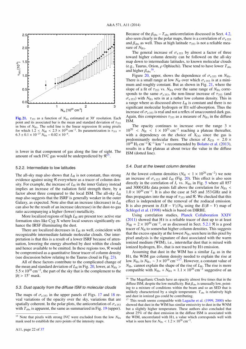
A&A 571, A11 (2014)

0 1 2 3NHI [1020 cm-2]

0.0

0.5

1.0

1.5

2.0

2.5

o 353

[10-6

]

Fig. 21. τ353 as a function of NH estimated at 30′ resolution. Eachpoint and its associated bar is the mean and standard deviation of τ353in bins of NH . The solid line is the linear regression fit using pixelsfor which 1.2 < NHI < 2.5 × 1020 cm−2. Its parametrization is τ353 =6.3 ± 0.1 × 10−27 NH − 0.02 × 10−6.

is lower in that component of gas along the line of sight. Theamount of such IVC gas would be underpredicted by R15.

5.2.2. Intermediate to low latitudes

The all-sky map also shows that LH is not constant, thus strongevidence against using R everywhere as a tracer of column den-sity. For example, the increase of LH in the inner Galaxy insteadimplies an increase of the radiation field strength there, by afactor about three compared to the local ISM. The all-sky LHmap also suggests that the ISRF is generally weaker in the outerGalaxy, as expected. Note also that an increase (decrease) in LHcan also be the result of an increase (decrease) in the dust-to-gasratio accompanying a higher (lower) metallicity.

More localized regions of high LH are present too: active starformation sites like Cyg X where local sources significantly en-hance the IRSF illuminating the dust.

There are localized decreases in LH as well, coincident withrecognizable intermediate-latitude molecular clouds. Our inter-pretation is that this is a result of a lower ISRF because of atten-uation, lowering the energy absorbed by dust within the cloudsand hence available to be emitted. In these regions too, R wouldbe compromised as a quantitative linear tracer of column density(see discussion below relating to the Taurus cloud in Fig. 23).

All of these factors contribute to the complicated change ofthe mean and standard deviation of LH in Fig. 20, lower, at NH >5.5× 1020 cm−2, the part of the sky that is the complement to the|b| > 15◦ mask.

5.3. Dust opacity from the diffuse ISM to molecular clouds

The maps of σe 353 in the upper panels of Figs. 17 and 18 re-veal variations of the opacity over the sky, variations that arespatially coherent. In the polar plots, the anticorrelation of σe 353with Tobs is apparent, the same as summarized in Fig. 19 (upper).

15 Note that pixels with strong IVC were excluded from the low NH mask used to establish the zero points of the intensity maps.

Because of the βobs − Tobs anticorrelation discussed in Sect. 4.2,also seen clearly in the polar maps, there is a correlation of σe 353and βobs as well. Thus at high latitude τ353 is not a reliable mea-sure of NH .

The general increase of σe 353 by almost a factor of threetoward higher column density can be followed on the all-skymap down to intermediate latitudes, to known molecular clouds(e.g., Taurus, Orion, ρ Ophiuchi). These tend to have lower Tobsand higher βobs

16.Figure 20, upper, shows the dependence of σe 353 on NH .

There is a small range at low NH over which σe 353 is at a mini-mum and roughly constant. But as shown in Fig. 21, where theslope of a fit of τ353 vs. NH over the same range of NH corre-sponds to the same σe 353, the non-linear increase of τ353 (andσe 353) with NH sets in at a rather low column density. This ina range where as discussed above LH is constant and there is nosignificant molecular hydrogen or H self-absorption. Thus theincrease ofσe 353 is real and not a reflex of unaccounted dark gas.Again, this compromises τ353 as a measure of NH in the diffuseISM.

The opacity continues to increase over the range 3 ×1020 < NH < 1 × 1021 cm−2 reaching a plateau thereafter,with a dependency on the choice of XCO since the gas ispredominantly molecular there. The choice of XCO = 2.0 ×1020 H2 cm−2 K−1 km−1 s recommended by Bolatto et al. (2013),results in a flat plateau at about twice the value in the diffuseISM (dotted line).

5.4. Dust at the lowest column densities

At the lowest column densities (NH < 1 × 1020 cm−2) we notean increase of σe 353 and LH (Fig. 20). This effect is also seendirectly in the correlation of Iν vs. NH in Fig. 5 where all 857and 3000 GHz data points fall above the correlation for NH <1.0 × 1020 cm−2. It is also the case at 545 and 353 GHz and itthus propagates into the map of τ353 and R. We checked that thiseffect is independent of the removal of the zodiacal emission.It is also present in E(B − V)/NH using the E(B − V) map ofSchlegel et al. (1998) which is based on DIRBE.

Using correlation studies, Planck Collaboration XXIV(2011) showed that H is a reliable tracer of dust up to at leastNHI = 2 × 1020 cm−2, or as discussed in Sect. 5.2.1 R is a goodtracer of NH to somewhat higher column densities. This suggeststhat the excess opacity at the lowest NH seen here in this pixel bypixel analysis is the signature of dust associated with the warmionized medium (WIM), i.e., interstellar dust that is mixed withionized hydrogen, H+, that is not traced by H emission.

Assuming that dust in the WIM has a similar LH as in theH , the WIM gas column density needed to explain the rise atlow NH is NH+ ∼ 3× 1019 cm−217. However, a constant value ofNH+ cannot explain the shape of the rise of LH. The rise is morecompatible with NH+ + NH ≈ 1.1 × 1020 cm−2 suggestive of an

16 The Magellanic Clouds have an opacity almost five times that in thediffuse ISM, despite the low metallicity. But βobs is unusually low, point-ing to a mixture of conditions within the beam and so an SED that isunlikely characterized by a single temperature. Tobs is relatively highand dust in ionized gas could be contributing.17 This result seems compatible with Lagache et al. (1999, 2000) whoshowed that dust in the WIM has similar emissivity to dust in the WNMbut a slightly higher temperature. These authors also concluded thatabout 25% of the dust emission in the diffuse ISM is associated withthe WIM, uncorrelated with H , a value which corresponds well withwhat is seen here for NH < 1.2 × 1020 cm−2.

A11, page 22 of 37

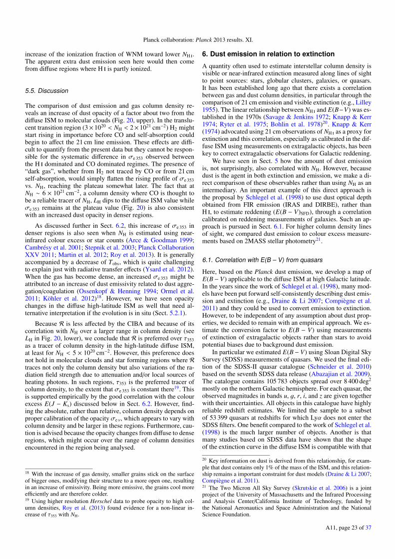
Planck collaboration: Planck 2013 results. XI.

increase of the ionization fraction of WNM toward lower NH .The apparent extra dust emission seen here would then comefrom diffuse regions where H is partly ionized.

5.5. Discussion

The comparison of dust emission and gas column density re-veals an increase of dust opacity of a factor about two from thediffuse ISM to molecular clouds (Fig. 20, upper). In the translu-cent transition region (3× 1020 < NH < 2× 1021 cm−2) H2 mightstart rising in importance before CO and self-absorption couldbegin to affect the 21 cm line emission. These effects are diffi-cult to quantify from the present data but they cannot be respon-sible for the systematic difference in σe 353 observed betweenthe H dominated and CO dominated regimes. The presence of“dark gas”, whether from H2 not traced by CO or from 21 cmself-absorption, would simply flatten the rising profile of σe 353vs. NH, reaching the plateau somewhat later. The fact that atNH ∼ 6 × 1021 cm−2, a column density where CO is thought tobe a reliable tracer of NH, LH dips to the diffuse ISM value whileσe 353 remains at the plateau value (Fig. 20) is also consistentwith an increased dust opacity in denser regions.

As discussed further in Sect. 6.2, this increase of σe 353 indenser regions is also seen when NH is estimated using near-infrared colour excess or star counts (Arce & Goodman 1999;Cambrésy et al. 2001; Stepnik et al. 2003; Planck CollaborationXXV 2011; Martin et al. 2012; Roy et al. 2013). It is generallyaccompanied by a decrease of Tobs, which is quite challengingto explain just with radiative transfer effects (Ysard et al. 2012).When the gas has become dense, an increased σe 353 might beattributed to an increase of dust emissivity related to dust aggre-gation/coagulation (Ossenkopf & Henning 1994; Ormel et al.2011; Köhler et al. 2012)18. However, we have seen opacitychanges in the diffuse high-latitude ISM as well that need al-ternative interpretation if the evolution is in situ (Sect. 5.2.1).

Because R is less affected by the CIBA and because of itscorrelation with NH over a larger range in column density (seeLH in Fig. 20, lower), we conclude that R is preferred over τ353as a tracer of column density in the high-latitude diffuse ISM,at least for NH < 5 × 1020 cm−2. However, this preference doesnot hold in molecular clouds and star forming regions where Rtraces not only the column density but also variations of the ra-diation field strength due to attenuation and/or local sources ofheating photons. In such regions, τ353 is the preferred tracer ofcolumn density, to the extent that σe 353 is constant there19. Thisis supported empirically by the good correlation with the colourexcess E(J − Ks) discussed below in Sect. 6.2. However, find-ing the absolute, rather than relative, column density depends onproper calibration of the opacity σe ν, which appears to vary withcolumn density and be larger in these regions. Furthermore, cau-tion is advised because the opacity changes from diffuse to denseregions, which might occur over the range of column densitiesencountered in the region being analysed.

18 With the increase of gas density, smaller grains stick on the surfaceof bigger ones, modifying their structure to a more open one, resultingin an increase of emissivity. Being more emissive, the grains cool moreefficiently and are therefore colder.19 Using higher resolution Herschel data to probe opacity to high col-umn densities, Roy et al. (2013) found evidence for a non-linear in-crease of τ353 with NH.

6. Dust emission in relation to extinction

A quantity often used to estimate interstellar column density isvisible or near-infrared extinction measured along lines of sightto point sources: stars, globular clusters, galaxies, or quasars.It has been established long ago that there exists a correlationbetween gas and dust column densities, in particular through thecomparison of 21 cm emission and visible extinction (e.g., Lilley1955). The linear relationship between NH and E(B−V) was es-tablished in the 1970s (Savage & Jenkins 1972; Knapp & Kerr1974; Ryter et al. 1975; Bohlin et al. 1978)20. Knapp & Kerr(1974) advocated using 21 cm observations of NH as a proxy forextinction and this correlation, especially as calibrated in the dif-fuse ISM using measurements on extragalactic objects, has beenkey to correct extragalactic observations for Galactic reddening.

We have seen in Sect. 5 how the amount of dust emissionis, not surprisingly, also correlated with NH. However, becausedust is the agent in both extinction and emission, we make a di-rect comparison of these observables rather than using NH as anintermediary. An important example of this direct approach isthe proposal by Schlegel et al. (1998) to use dust optical depthobtained from FIR emission (IRAS and DIRBE), rather thanH , to estimate reddening (E(B − V)SFD), through a correlationcalibrated on reddening measurements of galaxies. Such an ap-proach is pursued in Sect. 6.1. For higher column density linesof sight, we compared dust emission to colour excess measure-ments based on 2MASS stellar photometry21.

6.1. Correlation with E(B – V) from quasars

Here, based on the Planck dust emission, we develop a map ofE(B− V) applicable to the diffuse ISM at high Galactic latitude.In the years since the work of Schlegel et al. (1998), many mod-els have been put forward self-consistently describing dust emis-sion and extinction (e.g., Draine & Li 2007; Compiègne et al.2011) and they could be used to convert emission to extinction.However, to be independent of any assumption about dust prop-erties, we decided to remain with an empirical approach. We es-timate the conversion factor to E(B − V) using measurementsof extinction of extragalactic objects rather than stars to avoidpotential biases due to background dust emission.

In particular we estimated E(B− V) using Sloan Digital SkySurvey (SDSS) measurements of quasars. We used the final edi-tion of the SDSS-II quasar catalogue (Schneider et al. 2010)based on the seventh SDSS data release (Abazajian et al. 2009).The catalogue contains 105 783 objects spread over 8 400 deg2

mostly on the northern Galactic hemisphere. For each quasar, theobserved magnitudes in bands u, g, r, i, and z are given togetherwith their uncertainties. All objects in this catalogue have highlyreliable redshift estimates. We limited the sample to a subsetof 53 399 quasars at redshifts for which Lyα does not enter theSDSS filters. One benefit compared to the work of Schlegel et al.(1998) is the much larger number of objects. Another is thatmany studies based on SDSS data have shown that the shapeof the extinction curve in the diffuse ISM is compatible with that

20 Key information on dust is derived from this relationship, for exam-ple that dust contains only 1% of the mass of the ISM, and this relation-ship remains a important constraint for dust models (Draine & Li 2007;Compiègne et al. 2011).21 The Two Micron All Sky Survey (Skrutskie et al. 2006) is a jointproject of the University of Massachusetts and the Infrared Processingand Analysis Center/California Institute of Technology, funded bythe National Aeronautics and Space Administration and the NationalScience Foundation.

A11, page 23 of 37

A&A 571, A11 (2014)

for stars from Fitzpatrick (1999) with RV = 3.1 (Jones et al.2011; Schlafly & Finkbeiner 2011; Mörtsell 2013), so that wecan take advantage of all of the multi-colour measurements. Thedetails of how we estimate E(B−V) for each quasar are given inAppendix E.

The correlations of E(B − V) with Planck R and τ353, fromwhich point sources have been removed (Sect. 3.4), are shownin Fig. 2222. Each is strongly correlated: E(B − V)/R = (5.40 ±0.09)×105 and E(B−V)/τ353 = (1.49±0.03)×104. The fractionaluncertainty of the slope of the correlation with R is about 20%lower than that for τ353. This is not unexpected, both from ourdiscussion of Fig. 13 and, in Sect. 5.2.1, of the factors that in-fluence τ353 but not R. This leads us to prefer the solution basedon R, E(B−V)R, to that based on τ353, E(B−V)τ353, for the lowcolumn density regions of the sky (see also Sect. 5.5).

The product of E(B−V)/R and the diffuse ISM estimates ofLH gives the ratio E(B−V)/NH = (1.42–1.46)×10−22 mag cm2, afactor just 0.82–0.85 lower than that measured using backgroundstars for lines of sight with considerably larger E(B−V) (Bohlinet al. 1978; Rachford et al. 2009). Given all the potential fordifferences, this agreement is remarkable. On the other hand, thesame ratio found using E(B−V)/τ353 and the low value of σe 353in Figs. 20, upper, and 21 and in Table 4 results in a factor 0.55–0.60 lower. Using the E(B − V) map derived from dust emissionτ3000 by Schlegel et al. (1998), Liszt (2014) also found a lowerratio, by a factor 0.7, for lines of sight with E(B − V) < 0.1.

6.2. Comparing to E(J – Ks) from star colours in molecularclouds

We have investigated how to estimate E(B−V) for nearby molec-ular clouds from Planck dust emission. A point of comparisonfor such regions is mapping of colour excesses E(J − H) andE(H − Ks), or their sum E(J − Ks), based on stellar colours(e.g., Goodman et al. 2009). Here we use maps produced withthe AvMAP technique and based on colour excesses from the2MASS data base (Schneider et al. 2011). Similar maps canbe obtained with the NICER and NICEST techniques (e.g.,Lombardi et al. 2011). The effective angular resolution of the2MASS extinction maps used here is a few minutes of arc (see,e.g., Roy et al. 2013), close to that of Planck.

Although the optical extinction is rarely directly measuredin the same high column density regions (Martin et al. 2012;Roy et al. 2013), these near-infrared colour excesses are usuallyexpressed as E(B − V)2MASS after conversion using an assumedshape of the extinction curve, that for stars with Rv = 3.1. Thisconversion might be inappropriate, and even variable across afield, because of dust evolution affecting all of the colour excessratios for a given column of dust. Nevertheless, it is still very in-teresting to compare the spatial details of the dust column den-sity revealed by dust extinction and by dust emission, becauseeach is affected by different systematic effects.

For the Taurus and ρ Ophiuchi molecular clouds, Figs. 23and 24 present a comparison of four different estimates of E(B−V): E(B − V)2MASS, E(B − V)τ353, E(B − V)SFD, and E(B − V)R.The Pearson correlation coefficients of E(B − V)2MASS with thethree other maps are given in Table 5. The correlation of E(B −V)τ353 map with E(B− V)2MASS is excellent (Pearson coefficientof 0.86 for Taurus and 0.95 for ρ Ophiuchi); this agreement is

22 Although not an explicit selection criterion, the range of τ353 sampledby the selected quasars corresponds the conditions in the low NH mask,Fig. 3, whose NDF for τ353 is shown in Fig. 6. The positions of the binsalong the x-axes in Fig. 22 reflect this NDF.

0 5 10 15 20R [10-8 W m-2 sr-1]

0.00

0.02

0.04

0.06

0.08

0.10

E(B-

V)

0 1 2 3 4 5 6o353 [10-6]

0.00

0.02

0.04

0.06

0.08

0.10

E(B-

V)

Fig. 22. E(B − V) measured with quasars in the diffuse ISM at highGalactic latitude as a function of R (upper) and τ353 (lower). Each pointis the average of E(B−V) values in a bin of τ353 or R. The bin size variesfor each bin such that there is always the same number of samples perbin (N = 1000). The error bar is the standard deviation of E(B − V)values in the bin, divided by

√N. The solid line is the linear regres-

sion fit to the whole sample; E(B − V)/R = (5.40 ± 0.09) × 105 andE(B−V)/τ353 = (1.49± 0.03)× 104. In each case, the intercept is small(–0.0040 for R and 0.0048 for τ353), in accordance with the fact that thezero levels of E(B−V) (i.e., the intrinsic colours) and of the Planck andIRIS data were estimated using a correlation with NH .

remarkable given that very different methods and data sets wereused to build these two maps. However, notice how the brightestfilamentary structures appear with more contrast in E(B−V)τ353than in E(B − V)2MASS, a point to which we shall return.

The Schlegel et al. (1998) map E(B − V)SFD was also pro-duced from a dust optical depth map (at 3000 GHz in that case;see Sect. 7.3 for details) and so the scale is similar. However, thecorrelation coefficient with E(B−V)2MASS is lower and it is clearthat a lot of spatial detail is absent. This arises because they esti-mated Tobs using the lower resolution DIRBE data, thus missingthe dust temperature decrease at small scales that accompaniesthe increase of column density in molecular clouds, and so theirmap of optical depth which underlies E(B − V)SFD has lowercontrast as well as lower resolution. Being able to follow thesmall-scale variations of Tobs appears to be essential to gaugeproperly the full structural details of the molecular clouds. This

A11, page 24 of 37

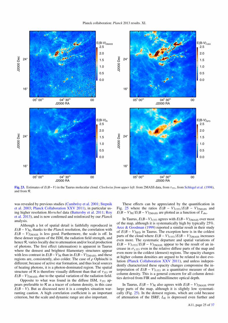
Planck collaboration: Planck 2013 results. XI.

05h 00m 04h 30m 00 J2000 RA

16°

24°

J200

0 D

ec

0.0

0.5

1.0

1.5

2.0

2.5E(B-V)2MASS

05h 00m 04h 30m 00 J2000 RA

16°

24°

J200

0 D

ec

0.0

0.5

1.0

1.5

2.0

2.5E(B-V)o353

05h 00m 04h 30m 00 J2000 RA

16°

24°

J200

0 D

ec

0.0

0.5

1.0

1.5

2.0

2.5E(B-V)R

05h 00m 04h 30m 00 J2000 RA

16°

24°

J200

0 D

ec

0.0

0.5

1.0

1.5

2.0

2.5E(B-V)SFD

Fig. 23. Estimates of E(B−V) in the Taurus molecular cloud. Clockwise from upper left: from 2MASS data, from τ353, from Schlegel et al. (1998),and from R.

was revealed by previous studies (Cambrésy et al. 2001; Stepniket al. 2003; Planck Collaboration XXV 2011), in particular us-ing higher resolution Herschel data (Battersby et al. 2011; Royet al. 2013), and is now confirmed and reinforced by our Planckanalysis.

Although a lot of spatial detail is faithfully reproduced inE(B − V)R, thanks to the Planck resolution, the correlation withE(B − V)2MASS is less good. Furthermore, the scale is off. Inthese denser regions of the ISM, the radiation field strength, andhenceR, varies locally due to attenuation and/or local productionof photons. The first effect (attenuation) is apparent in Tauruswhere the densest and brightest filamentary structures appearwith less contrast in E(B−V)R than in E(B−V)2MASS, and theseregions are, consistently, also colder. The case of ρ Ophiuchi isdifferent; because of active star formation, and thus local sourcesof heating photons, it is a photon-dominated region. The spatialstructure of R is therefore visually different than that of τ353 orE(B−V)2MASS, due to the spatial variation of the radiation field.

Opposite to what was found in the diffuse ISM, τ353 ap-pears preferable to R as a tracer of column density, in this caseE(B − V). But as discussed next it is a complex situation war-ranting caution. A high correlation coefficient is an importantcriterion, but the scale and dynamic range are also important.

These effects can be appreciated by the quantification inFig. 25 where the ratios E(B − V)τ353/E(B − V)2MASS andE(B − V)R/E(B − V)2MASS are plotted as a function of Tobs.

In Taurus, E(B−V)τ353 agrees with E(B−V)2MASS over mostof the map, although it is systematically high by typically 25%.Arce & Goodman (1999) reported a similar result in their studyof E(B − V)SFD in Taurus. The exception here is in the coldestparts of the cloud where E(B − V)τ353/E(B − V)2MASS increaseseven more. The systematic departure and spatial variations ofE(B − V)τ353/E(B − V)2MASS appear to be the result of an in-crease in σe 353 even in the relative diffuse parts of the map andeven more in the coldest (densest) regions. The opacity changesat higher column densities are argued to be related to dust evo-lution (Planck Collaboration XXV 2011), and unless indepen-dently characterized these opacity changes compromise the in-terpretation of E(B − V)τ353 as a quantitative measure of dustcolumn density. This is a general concern for all column densi-ties derived from FIR and submillimetre optical depth.

In Taurus, E(B − V)R also agrees with E(B − V)2MASS overlarge parts of the map, although it is slightly low systemati-cally (Fig. 25). In the densest regions, which are cold becauseof attenuation of the ISRF, LH is depressed even further and

A11, page 25 of 37

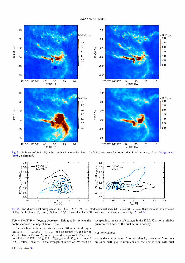
A&A 571, A11 (2014)

17h 00m 16h 50m 40 30 20 10 J2000 RA

-28°

-26°

-24°

-22°

-20°

-18°

J200

0 D

ec

0.00.51.01.52.02.53.0

E(B-V)2MASS

17h 00m 16h 50m 40 30 20 10 J2000 RA

-28°

-26°

-24°

-22°

-20°

-18°

J200

0 D

ec

0.00.51.01.52.02.53.0

E(B-V)o353

17h 00m 16h 50m 40 30 20 10 J2000 RA

-28°

-26°

-24°

-22°

-20°

-18°

J200

0 D

ec

0.00.51.01.52.02.53.0

E(B-V)R

17h 00m 16h 50m 40 30 20 10 J2000 RA

-28°

-26°

-24°

-22°

-20°

-18° J2

000

Dec

0.00.51.01.52.02.53.0

E(B-V)SFD

Fig. 24. Estimates of E(B − V) in the ρ Ophiuchi molecular cloud. Clockwise from upper left: from 2MASS data, from τ353, from Schlegel et al.(1998), and from R.

14 15 16 17 18 19 20Tobs [K]

0.00.5

1.0

1.5

2.0

2.5

3.03.5

E(B-

V)Pl

anck

/ E(

B-V)

2MAS

S E(B-V)o 353E(B-V)R

17 18 19 20 21 22 23Tobs [K]

0.00.5

1.0

1.5

2.0

2.5

3.03.5

E(B-

V)Pl

anck

/ E(

B-V)

2MAS

S E(B-V)o 353E(B-V)R

Fig. 25. Two-dimensional histogram of E(B−V)τ353/E(B−V)2MASS (black contours) and E(B−V)R/E(B−V)2MASS (blue contours) as a functionof Tobs, for the Taurus (left) and ρ Ophiuchi (right) molecular clouds. The maps used are those shown in Figs. 23 and 24.

E(B − V)R/E(B − V)2MASS decreases. This greatly reduces thecontrast across the map of E(B − V)R.

In ρ Ophiuchi, there is a similar scale difference in the typ-ical E(B − V)τ353/E(B − V)2MASS and an upturn toward lowerTobs. Unlike in Taurus, LH is not generally depressed. There is acorrelation of E(B − V)R/E(B − V)2MASS with Tobs as expectedif Tobs reflects changes in the strength of radiation. Without an

independent measure of changes in the ISRF, R is not a reliablequantitative tracer of the dust column density.

6.3. Discussion

As in the comparison of column density measures from dustemission with gas column density, the comparison with dust

A11, page 26 of 37

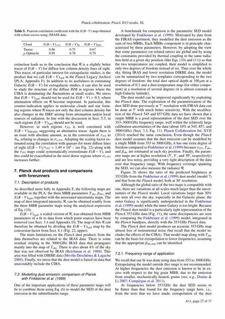
Planck collaboration: Planck 2013 results. XI.

Table 5. Pearson correlation coefficient with the E(B−V) map obtainedwith colour excess using 2MASS data.

Cloud E(B − V)τ353 E(B − V)R E(B − V)SFD

Taurus 0.86 0.75 0.67ρ Ophiuchi 0.95 0.70 0.79

extinction leads us to the conclusion that R is a slightly bettertracer of E(B − V) for diffuse low column density lines of sight.This tracer, of particular interest for extragalactic studies, is theproduct that we call E(B − V)xgal in the Planck Legacy Archive(PLA; Appendix F). In addition to its usefulness in estimatingGalactic E(B − V) for extragalactic studies, it can also be usedto study the structure of the diffuse ISM in regions where theCIBA is dominating the fluctuations at small scales. We stressthat E(B − V)xgal should not be used for E(B − V) > 0.3, whereattenuation effects on R become important. In particular, thiscounter-indication applies in molecular clouds and star form-ing regions where R traces not only the dust column density butalso changes in the ISRF arising from attenuation and/or localsources of radiation. In line with the discussion in Sect. 5.5, insuch regions E(B − V)xgal should not be used.

However, in such regions τ353 is well correlated withE(B − V)2MASS, suggesting an alternative tracer. Again there isan issue with absolute amount, as in the conversion of τ353 toNH, relating to changes in σe 353. Adopting the scaling factor es-timated using the correlation with quasars for more diffuse linesof sight (E(B − V)/τ353 = 1.49 × 104 – see Fig. 22) along withthe τ353 maps could systematically overestimate E(B − V), andthis could be exacerbated in the most dense regions where σe 353increases further.

7. Planck dust products and comparisonswith forerunners

7.1. Description of products

As described more fully in Appendix F, the following maps areavailable in the PLA: the three MBB parameters Tobs, βobs, andE(B−V)xgal, together with the associated uncertainty maps. Themap of dust integrated intensity, R, can be obtained readily fromthe three MBB parameter maps using the analytical expressionof Eq. (10).

E(B−V)xgal, a scaled version of R, was obtained from MBBparameters of a fit to data from which point sources have beenremoved (see Sect. 3.4 and Appendix D). The map of this R cantherefore be obtained by dividing the E(B − V)xgal map by theconversion factor from Sect. 6.1 (Fig. 22, upper).

The main limitations on the Planck dust products from thedata themselves are related to the IRAS data. There is someresidual striping in the 3000 GHz IRAS data that propagatesmainly into the map of Tobs. There is also about 4% of the skythat was not observed by IRAS (Beichman et al. 1988). Thisarea was filled with DIRBE data (Miville-Deschênes & Lagache2005). Finally, we stress that the dust model is based on data thatunavoidably include the CIBA.

7.2. Modelling dust emission: comparison of Planckwith Finkbeiner et al. (1999)

One of the important applications of these parameter maps willbe to combine them using Eq. (6) to model the SED of the dustemission in the submillimetre range.

A benchmark for comparison is the parametric SED modeldeveloped by Finkbeiner et al. (1999). Motivated by data fromthe FIRAS experiment, they modelled the dust emission as thesum of two MBBs. Each MBBs component is in principle char-acterized by three parameters. However, by adopting the viewthat some parameters (or related ratios) are global and by usingthe constraints provided by thermal coupling to the same radia-tion field at a given sky position (like Eqs. (10) and (11)) so thatthe two temperatures are coupled, their model is simplified toonly two degrees of freedom instead of six. Thus over the wholesky, fitting IRAS and lower resolution DIRBE data, the modelcan be summarized by two templates corresponding to the twodegrees of freedom: the total dust optical depth at 100 µm at aresolution of 6.′1 and a dust temperature map (for either compo-nent) at a resolution of several degrees (it is almost constant athigh Galactic latitude).

The dust model can be improved significantly by exploitingthe Planck data. The exploration of the parametrization of thedust SED done previously at 7◦ resolution with FIRAS data canbe done at 5′ with much better sensitivity. With the recalibra-tion of the Planck 545 and 857 GHz data we have shown that asingle MBB is a good representation of the dust SED over the353–3000 GHz frequency range, well within the relatively largecalibration uncertainties of the data (about 10% at 545, 857, and3000 GHz) (Sect. 3.3, Fig. 11). Planck Collaboration Int. XVII(2014) reached the same conclusion. Even though the Planckdust model assumes that the dust emission can be modelled bya single MBB from 353 to 3000 GHz, it has one extra degree offreedom compared to Finkbeiner et al. (1999) because τ353, Tobs,and βobs are estimated at each sky position. Finally, the param-eter maps are at higher resolution (5′, 5′, and 30′, respectively)and are less noisy, providing a very tight description of the dataover that frequency range. With frequency coverage spanningthe SED, we can also measure the radiance R.

Figure 26 shows the ratio of the predicted brightness at353 GHz from the Finkbeiner et al. (1999) dust model (model 7)and that from the Planck model, both at 30′ resolution.

Although the global ratio of the two maps is compatible withone, there are variations at all scales much larger than the uncer-tainties of the Planck model. Local variations larger than 30%are seen all over the sky, especially in the Galactic plane; theouter Galaxy is significantly underpredicted in the Finkbeineret al. (1999) model while the inner Galaxy is too bright. Becausethe Planck dust model is a particularly tight representation of thePlanck 353 GHz data (Fig. 11), the same discrepancies are seenby comparing the Finkbeiner et al. (1999) model, integrated inthe Planck bandpass, directly with the 353 GHz Planck data.

The Planck dust model produces an accurate 353 GHz mapalmost free of instrumental noise (but recall that the model in-cludes the effects of the CIBA). That model map along with Tobscan be the basis for extrapolation to lower frequencies, assumingthat the appropriate βobs,mm can be identified.

7.2.1. Frequency range of application

We recall that our fit was done using data from 353 to 3000 GHz.Extrapolating the model outside this range is not recommended.At higher frequencies the dust emission is known to be in ex-cess with respect to the big grain MBB, due to the emissionfrom smaller, stochastically heated, grains (see, e.g., Draine &Li 2007; Compiègne et al. 2011).

At frequencies below 353 GHz the dust SED seems tobe flatter than that found for the frequency range here, i.e.,from the tests that we have made, extrapolation of the dust

A11, page 27 of 37

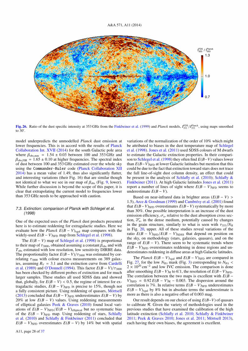
A&A 571, A11 (2014)

0.7

1.0

1.3IFDS / IPlanck353 353

Fig. 26. Ratio of the dust specific intensity at 353 GHz from the Finkbeiner et al. (1999) and Planck models, IFDS353 /I

Planck353 , using maps smoothed

to 30′.

model underpredicts the unmodelled Planck dust emission atlower frequencies. This is in accord with the results of PlanckCollaboration Int. XVII (2014) for the south Galactic pole areawhere βobs,mm = 1.54 ± 0.03 between 100 and 353 GHz andβobs,FIR = 1.65 ± 0.10 at higher frequencies. The spectral indexof dust between 100 and 353 GHz estimated over the whole skyusing the Commander-Ruler code (Planck Collaboration XII2014) has a mean value of 1.49, thus also significantly flatter,and interesting variations (their Fig. 16) that are similar thoughnot identical to what we see in our map of βobs (Fig. 9, lower).While further discussion is beyond the scope of this paper, it isclear that extrapolating the current model to frequencies lowerthan 353 GHz needs to be approached with caution.

7.3. Extinction: comparison of Planck with Schlegel et al.(1998)

One of the expected uses of the Planck dust products presentedhere is to estimate reddening for extragalactic studies. Here weevaluate how the Planck E(B − V)xgal map compares with thewidely-used E(B − V)SFD map from Schlegel et al. (1998).

The E(B − V) map of Schlegel et al. (1998) is proportionalto their map of τ3000, obtained assuming a constant βobs and withTobs estimated with low resolution, low sensitivity DIRBE data.The proportionality factor E(B− V)/τ3000 was estimated by cor-relating τ3000 with colour excess measurements on 389 galax-ies, assuming RV = 3.1 and the extinction curve from Cardelliet al. (1989) and O’Donnell (1994). This factor E(B − V)/τ3000has been checked by different probes of extinction and for muchlarger samples. These studies all used SDSS data and showedthat, globally, for E(B − V) < 0.5, the regime of interest for ex-tragalactic studies, E(B − V)SFD is precise to 15%, though nota fully consistent picture. Using reddening of quasars, Mörtsell(2013) concluded that E(B − V)SFD underestimates E(B − V) by20% at low E(B − V) values. Using reddening measurementsof elliptical galaxies Peek & Graves (2010) found local vari-ations of E(B − V)SFD/E(B − V)elliptical but no systematic biasof the E(B − V)SFD map. Using reddening of stars, Schlaflyet al. (2010) and Schlafly & Finkbeiner (2011) concluded thatE(B − V)SFD overestimates E(B − V) by 14% but with spatial

variations of the normalization of the order of 10% which mightbe attributed to biases in the dust temperature map of Schlegelet al. (1998). Jones et al. (2011) used SDSS colours of M dwarfsto estimate the Galactic extinction properties. In their compari-son to Schlegel et al. (1998) they often find E(B−V) values lowerthan E(B−V)SFD at lower Galactic latitudes but mention that thiscould be due to the fact that extinction toward stars does not tracethe full line-of-sight dust column density, an effect that couldbe present in the analysis of Schlafly et al. (2010); Schlafly &Finkbeiner (2011). At high Galactic latitudes Jones et al. (2011)report a number of lines of sight where E(B − V)SFD seems tounderestimate E(B − V).

Based on near-infrared data in brighter areas (E(B − V) >1.5), Arce & Goodman (1999) and Cambrésy et al. (2001) foundthat E(B−V)SFD overestimates E(B−V) systematically by morethan 30%. One possible interpretation is an increase of the dustemission efficiency, σa, relative to the dust absorption cross sec-tion, σa, in the dense medium, potentially caused by changesin the grain structure, similarly to what is seen with τ353/NHin Fig. 20, upper. All of these studies reveal variations of theratio E(B − V)SFD/E(B − V)SDSS that depend on position onthe sky, on methodology (stars, galaxies, quasars), and on therange of E(B − V). There seem to be systematic trends whereE(B − V)SFD overestimates reddening in dense regions and un-derestimates reddening in diffuse areas at high Galactic latitudes.

The Planck E(B − V)xgal and E(B − V)SFD are compared inFig. 27, for the low NH mask (Fig. 3) corresponding to NH <2 × 1020 cm−2 and low IVC emission. The comparison is doneafter smoothing E(B−V)R to 6.′1, the resolution of E(B−V)SFD.The correlation between the two maps is excellent with E(B −V)SFD = 0.92 E(B − V)R − 0.003. The dispersion around thecorrelation is 7%. In relative terms E(B − V)SFD underestimatesE(B − V)xgal by 8% but in absolute terms the underestimate ismore as there is also a negative offset of 0.003 mag.

Our result depends on our choice of using E(B−V) of quasarsto calibrate R. Given the variety of methodologies used in theprevious studies that have examined the calibration of the highlatitude extinction (Schlafly et al. 2010; Schlafly & Finkbeiner2011; Peek & Graves 2010; Jones et al. 2011; Mörtsell 2013),each having their own biases, the agreement is excellent.

A11, page 28 of 37

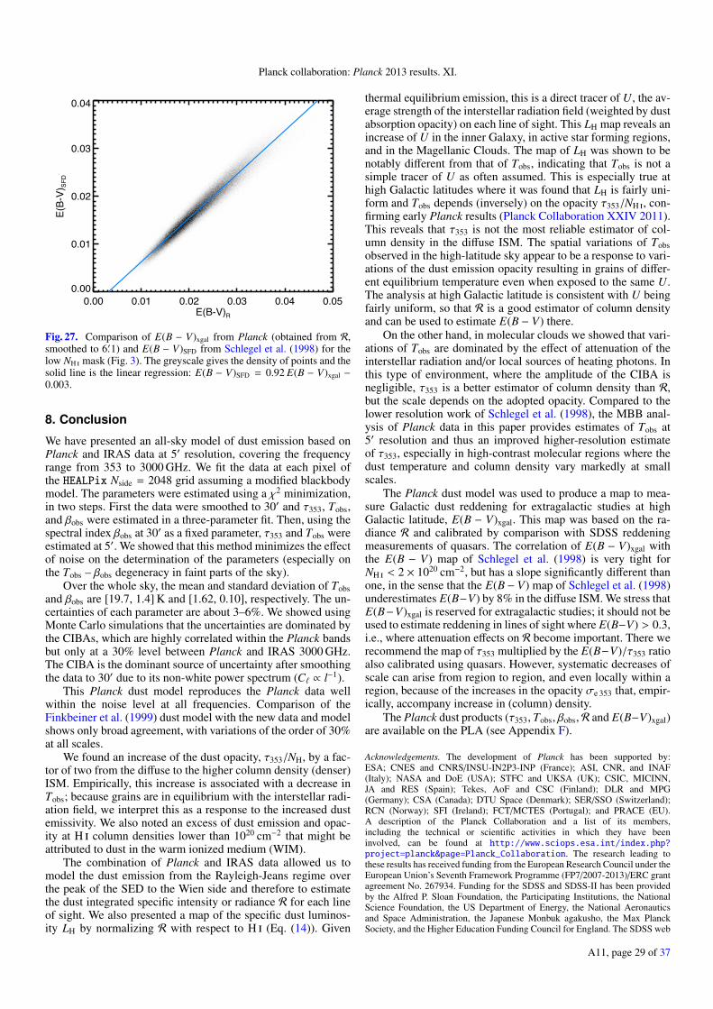
Planck collaboration: Planck 2013 results. XI.

0.00 0.01 0.02 0.03 0.04 0.05E(B-V)R

0.00

0.01

0.02

0.03

0.04

E(B-V)

SFD

Fig. 27. Comparison of E(B − V)xgal from Planck (obtained from R,smoothed to 6.′1) and E(B − V)SFD from Schlegel et al. (1998) for thelow NH mask (Fig. 3). The greyscale gives the density of points and thesolid line is the linear regression: E(B − V)SFD = 0.92 E(B − V)xgal −

0.003.

8. Conclusion

We have presented an all-sky model of dust emission based onPlanck and IRAS data at 5′ resolution, covering the frequencyrange from 353 to 3000 GHz. We fit the data at each pixel ofthe HEALPix Nside = 2048 grid assuming a modified blackbodymodel. The parameters were estimated using a χ2 minimization,in two steps. First the data were smoothed to 30′ and τ353, Tobs,and βobs were estimated in a three-parameter fit. Then, using thespectral index βobs at 30′ as a fixed parameter, τ353 and Tobs wereestimated at 5′. We showed that this method minimizes the effectof noise on the determination of the parameters (especially onthe Tobs – βobs degeneracy in faint parts of the sky).

Over the whole sky, the mean and standard deviation of Tobsand βobs are [19.7, 1.4] K and [1.62, 0.10], respectively. The un-certainties of each parameter are about 3–6%. We showed usingMonte Carlo simulations that the uncertainties are dominated bythe CIBAs, which are highly correlated within the Planck bandsbut only at a 30% level between Planck and IRAS 3000 GHz.The CIBA is the dominant source of uncertainty after smoothingthe data to 30′ due to its non-white power spectrum (C` ∝ l−1).

This Planck dust model reproduces the Planck data wellwithin the noise level at all frequencies. Comparison of theFinkbeiner et al. (1999) dust model with the new data and modelshows only broad agreement, with variations of the order of 30%at all scales.

We found an increase of the dust opacity, τ353/NH, by a fac-tor of two from the diffuse to the higher column density (denser)ISM. Empirically, this increase is associated with a decrease inTobs; because grains are in equilibrium with the interstellar radi-ation field, we interpret this as a response to the increased dustemissivity. We also noted an excess of dust emission and opac-ity at H column densities lower than 1020 cm−2 that might beattributed to dust in the warm ionized medium (WIM).

The combination of Planck and IRAS data allowed us tomodel the dust emission from the Rayleigh-Jeans regime overthe peak of the SED to the Wien side and therefore to estimatethe dust integrated specific intensity or radiance R for each lineof sight. We also presented a map of the specific dust luminos-ity LH by normalizing R with respect to H (Eq. (14)). Given

thermal equilibrium emission, this is a direct tracer of U, the av-erage strength of the interstellar radiation field (weighted by dustabsorption opacity) on each line of sight. This LH map reveals anincrease of U in the inner Galaxy, in active star forming regions,and in the Magellanic Clouds. The map of LH was shown to benotably different from that of Tobs, indicating that Tobs is not asimple tracer of U as often assumed. This is especially true athigh Galactic latitudes where it was found that LH is fairly uni-form and Tobs depends (inversely) on the opacity τ353/NH , con-firming early Planck results (Planck Collaboration XXIV 2011).This reveals that τ353 is not the most reliable estimator of col-umn density in the diffuse ISM. The spatial variations of Tobsobserved in the high-latitude sky appear to be a response to vari-ations of the dust emission opacity resulting in grains of differ-ent equilibrium temperature even when exposed to the same U.The analysis at high Galactic latitude is consistent with U beingfairly uniform, so that R is a good estimator of column densityand can be used to estimate E(B − V) there.

On the other hand, in molecular clouds we showed that vari-ations of Tobs are dominated by the effect of attenuation of theinterstellar radiation and/or local sources of heating photons. Inthis type of environment, where the amplitude of the CIBA isnegligible, τ353 is a better estimator of column density than R,but the scale depends on the adopted opacity. Compared to thelower resolution work of Schlegel et al. (1998), the MBB anal-ysis of Planck data in this paper provides estimates of Tobs at5′ resolution and thus an improved higher-resolution estimateof τ353, especially in high-contrast molecular regions where thedust temperature and column density vary markedly at smallscales.

The Planck dust model was used to produce a map to mea-sure Galactic dust reddening for extragalactic studies at highGalactic latitude, E(B − V)xgal. This map was based on the ra-diance R and calibrated by comparison with SDSS reddeningmeasurements of quasars. The correlation of E(B − V)xgal withthe E(B − V) map of Schlegel et al. (1998) is very tight forNH < 2 × 1020 cm−2, but has a slope significantly different thanone, in the sense that the E(B − V) map of Schlegel et al. (1998)underestimates E(B−V) by 8% in the diffuse ISM. We stress thatE(B−V)xgal is reserved for extragalactic studies; it should not beused to estimate reddening in lines of sight where E(B−V) > 0.3,i.e., where attenuation effects on R become important. There werecommend the map of τ353 multiplied by the E(B−V)/τ353 ratioalso calibrated using quasars. However, systematic decreases ofscale can arise from region to region, and even locally within aregion, because of the increases in the opacity σe 353 that, empir-ically, accompany increase in (column) density.

The Planck dust products (τ353, Tobs, βobs,R and E(B−V)xgal)are available on the PLA (see Appendix F).

Acknowledgements. The development of Planck has been supported by:ESA; CNES and CNRS/INSU-IN2P3-INP (France); ASI, CNR, and INAF(Italy); NASA and DoE (USA); STFC and UKSA (UK); CSIC, MICINN,JA and RES (Spain); Tekes, AoF and CSC (Finland); DLR and MPG(Germany); CSA (Canada); DTU Space (Denmark); SER/SSO (Switzerland);RCN (Norway); SFI (Ireland); FCT/MCTES (Portugal); and PRACE (EU).A description of the Planck Collaboration and a list of its members,including the technical or scientific activities in which they have beeninvolved, can be found at http://www.sciops.esa.int/index.php?project=planck&page=Planck_Collaboration. The research leading tothese results has received funding from the European Research Council under theEuropean Union’s Seventh Framework Programme (FP7/2007-2013)/ERC grantagreement No. 267934. Funding for the SDSS and SDSS-II has been providedby the Alfred P. Sloan Foundation, the Participating Institutions, the NationalScience Foundation, the US Department of Energy, the National Aeronauticsand Space Administration, the Japanese Monbuk agakusho, the Max PlanckSociety, and the Higher Education Funding Council for England. The SDSS web

A11, page 29 of 37

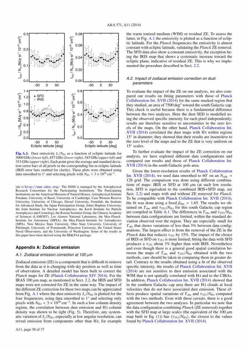
A&A 571, A11 (2014)

-50 0 50Ecliptic latitude [deg]

0.00.2

0.4

0.6

0.8

1.0

1.21.4

I 3000

/ N

HI [

MJy

sr-1

10-2

0 cm

2 ]

SFDIRIS

-50 0 50Ecliptic latitude [deg]

0.0

0.2

0.4

0.6

0.8

I 857 /

NH

I [M

Jy s

r-1 1

0-20 c

m2 ]

-50 0 500.0

0.1

0.2

0.3

I 545 /

NH

I [M

Jy s

r-1 1

0-20 c

m2 ]

-50 0 500.00

0.02

0.04

0.06

0.08

I 353 /

NH

I [M

Jy s

r-1 1

0-20 c

m2 ]

Fig. A.1. Dust emissivity Iν/NH as a function of ecliptic latitude for3000 GHz (lower left), 857 GHz (lower right), 545 GHz (upper left) and353 GHz (upper right). Each point gives the average and standard devia-tion (error bar) of all pixels in the corresponding bin in ecliptic latitude(IRIS error bars omitted for clarity). These plots were obtained usingdata smoothed to 1◦ and selecting pixels with NH < 3 × 1020 cm−2.

site is http://www.sdss.org/. The SDSS is managed by the AstrophysicalResearch Consortium for the Participating Institutions. The ParticipatingInstitutions are the American Museum of Natural History, Astrophysical InstitutePotsdam, University of Basel, University of Cambridge, Case Western ReserveUniversity, University of Chicago, Drexel University, Fermilab, the Institutefor Advanced Study, the Japan Participation Group, Johns Hopkins University,the Joint Institute for Nuclear Astrophysics, the Kavli Institute for ParticleAstrophysics and Cosmology, the Korean Scientist Group, the Chinese Academyof Sciences (LAMOST), Los Alamos National Laboratory, the Max-Planck-Institute for Astronomy (MPIA), the Max-Planck-Institute for Astrophysics(MPA), New Mexico State University, Ohio State University, University ofPittsburgh, University of Portsmouth, Princeton University, the United StatesNaval Observatory, and the University of Washington. Some of the results inthis paper have been derived using the HEALPix package.

Appendix A: Zodiacal emission

A.1. Zodiacal emission correction at 100 µm

Zodiacal emission (ZE) is a component that is difficult to removefrom the data as it is changing with sky position as well as timeof observation. A detailed model has been built to correct thePlanck maps for ZE (Planck Collaboration XIV 2014). For theIRAS 100 µm map, as mentioned in Sect. 2.2, the IRIS and SFDmaps were not corrected for ZE in the same way. The impact ofthe different ZE correction for these two maps can be appreciatedfrom Fig. A.1 where the dust emissivity Iν/NH is plotted for thefour frequencies, using data smoothed to 1◦ and selecting onlypixels with NH < 3 × 1020 cm−2. In such a low column densityregime, the correlation between dust emission and H columndensity was shown to be tight (Fig. 5). Therefore, any system-atic variation of Iν/NH , especially at low angular resolution, canreveal emission from components other than H , for example

the warm ionized medium (WIM) or residual ZE. To assess thelatter, in Fig. A.1 the emissivity is plotted as a function of eclip-tic latitude. For the Planck frequencies the emissivity is almostconstant with ecliptic latitude, validating the Planck ZE removal.The SFD data also show a constant emissivity, the exception be-ing the IRIS map that shows a systematic increase toward theecliptic plane, indicative of residual ZE. This is why we imple-mented the procedure described in Sect. 2.2.

A.2. Impact of zodiacal emission correction on dustparameters

To evaluate the impact of the ZE on our analysis, we also com-pared our results on fitting parameters with those of PlanckCollaboration Int. XVII (2014) for the same masked region thatthey studied, an area of 7500 deg2 toward the south Galactic cap.This check is useful because there is a fundamental differencebetween the two analyses. Here the dust SED is modelled us-ing the observed specific intensity for each pixel independently;results are therefore sensitive to uncertainties in the zero lev-els of the maps. On the other hand, Planck Collaboration Int.XVII (2014) correlated the dust maps with H within regions15◦ in diameter; they showed that their results are insensitive tothe zero level of the maps and to the ZE that is very uniform on15◦ scales.

To further evaluate the impact of the ZE correction on ouranalysis, we have explored different data configurations andcompared our results and those of Planck Collaboration Int.XVII (2014) in the south Galactic pole area.

Given the lower-resolution results of Planck CollaborationInt. XVII (2014), we used data smoothed to 60′ on an Nside =128 grid. The comparison was done using different combina-tions of maps: IRIS or SFD at 100 µm (at such low resolu-tion, SFD is equivalent to the combined IRIS+SFD map, seeSect. 2.2) and maps with and without ZE removed for Planck.To be compatible with Planck Collaboration Int. XVII (2014),the fit was done using a fixed βobs = 1.65. The results we ob-tained on Tobs and τ353/NH for this south Galactic cap regionare compiled in Table A.1. The differences in Tobs and τ353/NH between data configurations are limited, within the standard de-viation observed over the region. They are especially small forTobs that shows variations of less than 5% between data config-urations. The largest effect is from the removal of the ZE in thePlanck data that reduces τ353 by 15%. The impact of the choiceof IRIS or SFD on τ353 is more limited; fitting the data with SFDproduces a τ353 about 3% higher than with IRIS. Neverthelessand even though there is a general good spatial correlation be-tween the maps of Tobs and τ353/NH obtained with the twomethods, care should be taken in comparing them in greater de-tail. Contrary to the results obtained using a fit of the observedspecific intensity, the results of Planck Collaboration Int. XVII(2014) are not sensitive to dust emission associated with theWIM that is not spatially correlated with H and to the CIBAs.In addition, Planck Collaboration Int. XVII (2014) showed thatin the southern Galactic cap area there are H clouds at localvelocities that do not have associated dust emission. These ef-fects produce spatial variations of Tobs and τ353/NH computedwith the two methods. Even with these caveats, there is a goodagreement between the two analyses. In particular we note thatthe data configuration combining Planck (ZE removed) togetherwith the SFD map at large scales (the equivalent of the 100 µmmap built in Eq. (1)) has 〈τ353/NH 〉, the closest to the valuesfound by Planck Collaboration Int. XVII (2014).

A11, page 30 of 37

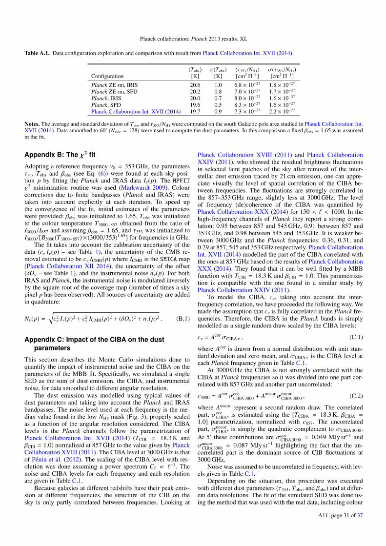
Planck collaboration: Planck 2013 results. XI.

Table A.1. Data configuration exploration and comparison with result from Planck Collaboration Int. XVII (2014).

〈Tobs〉 σ(Tobs) 〈τ353/NH 〉 σ(τ353/NH )Configuration [K] [K] [cm2 H−1] [cm2 H−1]

Planck ZE rm, IRIS 20.6 1.0 6.8 × 10−27 1.8 × 10−27

Planck ZE rm, SFD 20.2 0.8 7.0 × 10−27 1.7 × 10−27

Planck, IRIS 20.0 0.7 8.0 × 10−27 1.6 × 10−27

Planck, SFD 19.6 0.5 8.3 × 10−27 1.6 × 10−27

Planck Collaboration Int. XVII (2014) 19.7 0.9 7.3 × 10−27 2.2 × 10−27

Notes. The average and standard deviation of Tobs and τ353/NH were computed on the south Galactic pole area studied in Planck Collaboration Int.XVII (2014). Data smoothed to 60′ (Nside = 128) were used to compute the dust parameters. In this comparison a fixed βobs = 1.65 was assumedin the fit.

Appendix B: The χ2 fit

Adopting a reference frequency ν0 = 353 GHz, the parametersτν0 , Tobs and βobs (see Eq. (6)) were found at each sky posi-tion p by fitting the Planck and IRAS data Iν(p). The MPFITχ2 minimization routine was used (Markwardt 2009). Colourcorrections due to finite bandpasses (Planck and IRAS) weretaken into account explicitly at each iteration. To speed upthe convergence of the fit, initial estimates of the parameterswere provided: βobs was initialized to 1.65, Tobs was initializedto the colour temperature T3000−857 obtained from the ratio ofI3000/I857 and assuming βobs = 1.65, and τ353 was initialized toI3000/[B3000(T3000−857)× (3000/353)1.65] for frequencies in GHz.

The fit takes into account the calibration uncertainty of thedata (cν Iν(p) – see Table 1), the uncertainty of the CMB re-moval estimated to be cν ICMB(p) where ICMB is the SMICA map(Planck Collaboration XII 2014), the uncertainty of the offset(δOν – see Table 1), and the instrumental noise nν(p). For bothIRAS and Planck, the instrumental noise is modulated inverselyby the square root of the coverage map (number of times a skypixel p has been observed). All sources of uncertainty are addedin quadrature:

Nν(p) =

√c2ν Iν(p)2 + c2

ν ICMB(p)2 + (δOν)2 + nν(p)2 . (B.1)

Appendix C: Impact of the CIBA on the dustparameters

This section describes the Monte Carlo simulations done toquantify the impact of instrumental noise and the CIBA on theparameters of the MBB fit. Specifically, we simulated a singleSED as the sum of dust emission, the CIBA, and instrumentalnoise, for data smoothed to different angular resolution.

The dust emission was modelled using typical values ofdust parameters and taking into account the Planck and IRASbandpasses. The noise level used at each frequency is the me-dian value found in the low NH mask (Fig. 3), properly scaledas a function of the angular resolution considered. The CIBAlevels in the Planck channels follow the parametrization ofPlanck Collaboration Int. XVII (2014) (TCIB = 18.3 K andβCIB = 1.0) normalized at 857 GHz to the value given by PlanckCollaboration XVIII (2011). The CIBA level at 3000 GHz is thatof Pénin et al. (2012). The scaling of the CIBA level with res-olution was done assuming a power spectrum C` ∝ `−1. Thenoise and CIBA levels for each frequency and each resolutionare given in Table C.1.

Because galaxies at different redshifts have their peak emis-sion at different frequencies, the structure of the CIB on thesky is only partly correlated between frequencies. Looking at

Planck Collaboration XVIII (2011) and Planck CollaborationXXIV (2011), who showed the residual brightness fluctuationsin selected faint patches of the sky after removal of the inter-stellar dust emission traced by 21 cm emission, one can appre-ciate visually the level of spatial correlation of the CIBA be-tween frequencies. The fluctuations are strongly correlated inthe 857–353 GHz range, slightly less at 3000 GHz. The levelof frequency (de)coherence of the CIBA was quantified byPlanck Collaboration XXX (2014) for 150 < ` < 1000. In thehigh-frequency channels of Planck they report a strong corre-lation: 0.95 between 857 and 545 GHz, 0.91 between 857 and353 GHz, and 0.98 between 545 and 353 GHz. It is weaker be-tween 3000 GHz and the Planck frequencies: 0.36, 0.31, and0.29 at 857, 545 and 353 GHz respectively. Planck CollaborationInt. XVII (2014) modelled the part of the CIBA correlated withthe ones at 857 GHz based on the results of Planck CollaborationXXX (2014). They found that it can be well fitted by a MBBfunction with TCIB = 18.3 K and βCIB = 1.0. This parametriza-tion is compatible with the one found in a similar study byPlanck Collaboration XXIV (2011).

To model the CIBA, cν, taking into account the inter-frequency correlation, we have proceeded the following way. Wemade the assumption that cν is fully correlated in the Planck fre-quencies. Therefore, the CIBA in the Planck bands is simplymodelled as a single random draw scaled by the CIBA levels:

cν = Acor σCIBA ν , (C.1)

where Acor is drawn from a normal distribution with unit stan-dard deviation and zero mean, and σCIBA ν is the CIBA level ateach Planck frequency given in Table C.1.

At 3000 GHz the CIBA is not strongly correlated with theCIBA at Planck frequencies so it was divided into one part cor-related with 857 GHz and another part uncorrelated:

c3000 = Acor σcorCIBA 3000 + Auncor σuncor

CIBA 3000 , (C.2)

where Auncor represent a second random draw. The correlatedpart, σcor

CIBA, is estimated using the [TCIBA = 18.3 K, βCIBA =1.0] parametrization, normalized with c857. The uncorrelatedpart, σuncor

CIBA, is simply the quadratic complement to σCIBA 3000.At 5′ these contributions are σcor

CIBA 3000 = 0.049 MJy sr−1 andσuncor

CIBA 3000 = 0.087 MJy sr−1 highlighting the fact that the un-correlated part is the dominant source of CIB fluctuations at3000 GHz.

Noise was assumed to be uncorrelated in frequency, with lev-els given in Table C.1.

Depending on the situation, this procedure was executedwith different dust parameters (τ353, Tobs, and βobs) and at differ-ent data resolutions. The fit of the simulated SED was done us-ing the method that was used with the real data, including colour

A11, page 31 of 37

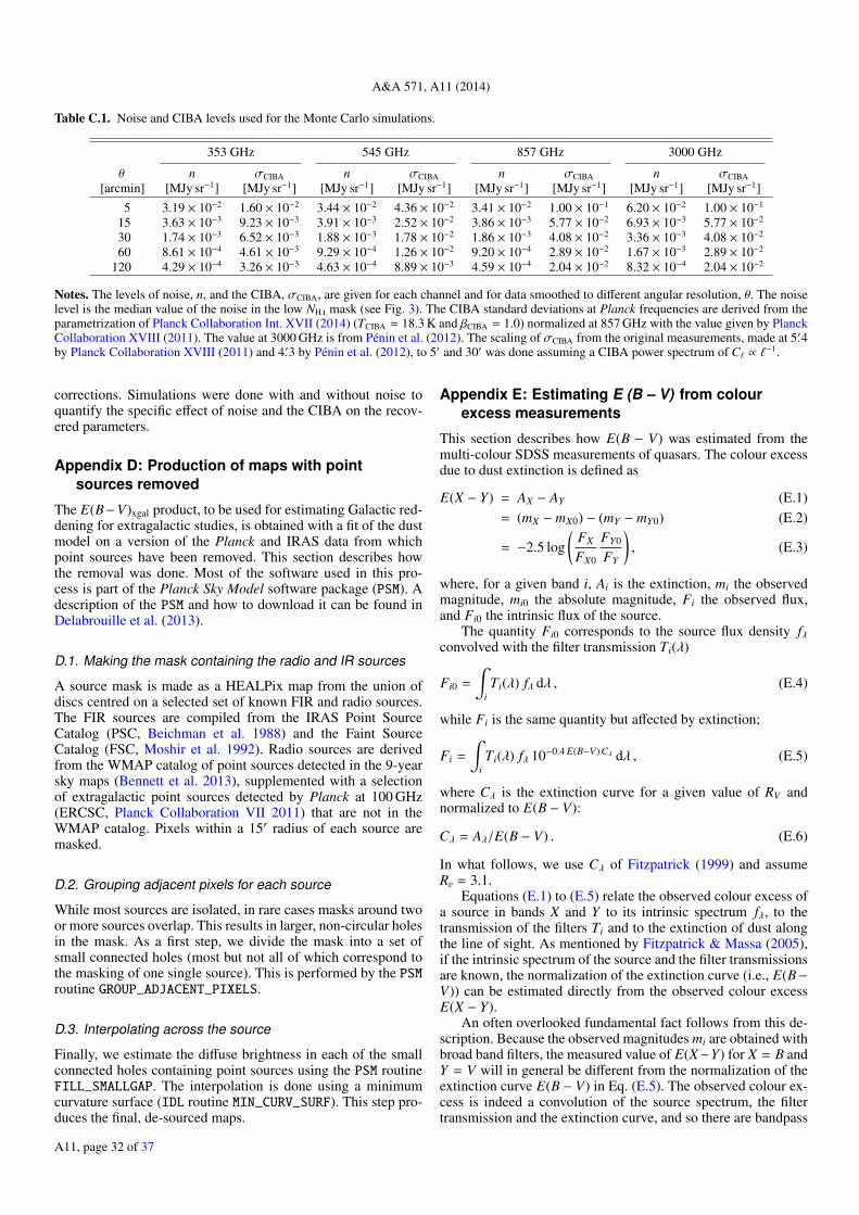
A&A 571, A11 (2014)

Table C.1. Noise and CIBA levels used for the Monte Carlo simulations.

353 GHz 545 GHz 857 GHz 3000 GHz

θ n σCIBA n σCIBA n σCIBA n σCIBA[arcmin] [MJy sr−1] [MJy sr−1] [MJy sr−1] [MJy sr−1] [MJy sr−1] [MJy sr−1] [MJy sr−1] [MJy sr−1]

5 3.19 × 10−2 1.60 × 10−2 3.44 × 10−2 4.36 × 10−2 3.41 × 10−2 1.00 × 10−1 6.20 × 10−2 1.00 × 10−1

15 3.63 × 10−3 9.23 × 10−3 3.91 × 10−3 2.52 × 10−2 3.86 × 10−3 5.77 × 10−2 6.93 × 10−3 5.77 × 10−2

30 1.74 × 10−3 6.52 × 10−3 1.88 × 10−3 1.78 × 10−2 1.86 × 10−3 4.08 × 10−2 3.36 × 10−3 4.08 × 10−2

60 8.61 × 10−4 4.61 × 10−3 9.29 × 10−4 1.26 × 10−2 9.20 × 10−4 2.89 × 10−2 1.67 × 10−3 2.89 × 10−2

120 4.29 × 10−4 3.26 × 10−3 4.63 × 10−4 8.89 × 10−3 4.59 × 10−4 2.04 × 10−2 8.32 × 10−4 2.04 × 10−2

Notes. The levels of noise, n, and the CIBA, σCIBA, are given for each channel and for data smoothed to different angular resolution, θ. The noiselevel is the median value of the noise in the low NH mask (see Fig. 3). The CIBA standard deviations at Planck frequencies are derived from theparametrization of Planck Collaboration Int. XVII (2014) (TCIBA = 18.3 K and βCIBA = 1.0) normalized at 857 GHz with the value given by PlanckCollaboration XVIII (2011). The value at 3000 GHz is from Pénin et al. (2012). The scaling of σCIBA from the original measurements, made at 5.′4by Planck Collaboration XVIII (2011) and 4.′3 by Pénin et al. (2012), to 5′ and 30′ was done assuming a CIBA power spectrum of C` ∝ `

−1.

corrections. Simulations were done with and without noise toquantify the specific effect of noise and the CIBA on the recov-ered parameters.

Appendix D: Production of maps with pointsources removed

The E(B−V)xgal product, to be used for estimating Galactic red-dening for extragalactic studies, is obtained with a fit of the dustmodel on a version of the Planck and IRAS data from whichpoint sources have been removed. This section describes howthe removal was done. Most of the software used in this pro-cess is part of the Planck Sky Model software package (PSM). Adescription of the PSM and how to download it can be found inDelabrouille et al. (2013).

D.1. Making the mask containing the radio and IR sources

A source mask is made as a HEALPix map from the union ofdiscs centred on a selected set of known FIR and radio sources.The FIR sources are compiled from the IRAS Point SourceCatalog (PSC, Beichman et al. 1988) and the Faint SourceCatalog (FSC, Moshir et al. 1992). Radio sources are derivedfrom the WMAP catalog of point sources detected in the 9-yearsky maps (Bennett et al. 2013), supplemented with a selectionof extragalactic point sources detected by Planck at 100 GHz(ERCSC, Planck Collaboration VII 2011) that are not in theWMAP catalog. Pixels within a 15′ radius of each source aremasked.

D.2. Grouping adjacent pixels for each source

While most sources are isolated, in rare cases masks around twoor more sources overlap. This results in larger, non-circular holesin the mask. As a first step, we divide the mask into a set ofsmall connected holes (most but not all of which correspond tothe masking of one single source). This is performed by the PSMroutine GROUP_ADJACENT_PIXELS.

D.3. Interpolating across the source

Finally, we estimate the diffuse brightness in each of the smallconnected holes containing point sources using the PSM routineFILL_SMALLGAP. The interpolation is done using a minimumcurvature surface (IDL routine MIN_CURV_SURF). This step pro-duces the final, de-sourced maps.

Appendix E: Estimating E (B – V) from colourexcess measurements

This section describes how E(B − V) was estimated from themulti-colour SDSS measurements of quasars. The colour excessdue to dust extinction is defined as

E(X − Y) = AX − AY (E.1)= (mX − mX0) − (mY − mY0) (E.2)

= −2.5 log(

FX

FX0

FY0

FY

), (E.3)

where, for a given band i, Ai is the extinction, mi the observedmagnitude, mi0 the absolute magnitude, Fi the observed flux,and Fi0 the intrinsic flux of the source.

The quantity Fi0 corresponds to the source flux density fλconvolved with the filter transmission Ti(λ)

Fi0 =

∫iTi(λ) fλ dλ , (E.4)

while Fi is the same quantity but affected by extinction;

Fi =

∫iTi(λ) fλ 10−0.4 E(B−V) Cλ dλ , (E.5)

where Cλ is the extinction curve for a given value of RV andnormalized to E(B − V):

Cλ = Aλ/E(B − V) . (E.6)

In what follows, we use Cλ of Fitzpatrick (1999) and assumeRv = 3.1.

Equations (E.1) to (E.5) relate the observed colour excess ofa source in bands X and Y to its intrinsic spectrum fλ, to thetransmission of the filters Ti and to the extinction of dust alongthe line of sight. As mentioned by Fitzpatrick & Massa (2005),if the intrinsic spectrum of the source and the filter transmissionsare known, the normalization of the extinction curve (i.e., E(B−V)) can be estimated directly from the observed colour excessE(X − Y).

An often overlooked fundamental fact follows from this de-scription. Because the observed magnitudes mi are obtained withbroad band filters, the measured value of E(X−Y) for X = B andY = V will in general be different from the normalization of theextinction curve E(B − V) in Eq. (E.5). The observed colour ex-cess is indeed a convolution of the source spectrum, the filtertransmission and the extinction curve, and so there are bandpass

A11, page 32 of 37

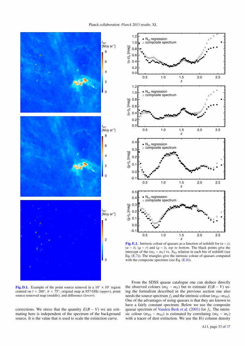
Planck collaboration: Planck 2013 results. XI.

0

2

4

6

8

I857[MJy sr-1]

0

2

4

6

8

I857[MJy sr-1]

0

2

4

I857[MJy sr-1]

Fig. D.1. Example of the point source removal in a 10◦ × 10◦ regioncentred on l = 260◦, b = 75◦; original map at 857 GHz (upper), pointsource removed map (middle), and difference (lower).

corrections. We stress that the quantity E(B − V) we are esti-mating here is independent of the spectrum of the backgroundsource. It is the value that is used to scale the extinction curve.

0.5 1.0 1.5 2.0 2.5z

0.00.2

0.4

0.6

0.8

1.0

1.2

(u-z

) 0 [m

ag]

NHI regressioncomposite spectrum

0.5 1.0 1.5 2.0 2.5z

0.00.2

0.4

0.6

0.8

1.01.2

(u-i)

0 [m

ag]

NHI regressioncomposite spectrum

0.5 1.0 1.5 2.0 2.5z

-0.1

0.0

0.1

0.2

0.3

0.4

(g-r)

0 [m

ag]

NHI regressioncomposite spectrum

0.5 1.0 1.5 2.0 2.5z

-0.10.0

0.1

0.2

0.3

0.40.5

(g-i)

0 [m

ag]

NHI regressioncomposite spectrum

Fig. E.1. Intrinsic colour of quasars as a function of redshift for (u− z),(u − i), (g − r) and (g − i), top to bottom. The black points give theintercept of the (mX − mY ) vs. NH relation in each bin of redshift (seeEq. (E.7)). The triangles give the intrinsic colour of quasars computedwith the composite spectrum (see Eq. (E.8)).

From the SDSS quasar catalogue one can deduce directlythe observed colours (mX − mY ) but to estimate E(B − V) us-ing the formalism described in the previous section one alsoneeds the source spectrum fλ and the intrinsic colour (mX0−mY0).One of the advantages of using quasars is that they are known tohave a fairly constant spectrum. Below we use the compositequasar spectrum of Vanden Berk et al. (2001) for fλ. The intrin-sic colour (mX0 − mY0) is estimated by correlating (mX − mY )with a tracer of dust extinction. We use the H column density

A11, page 33 of 37

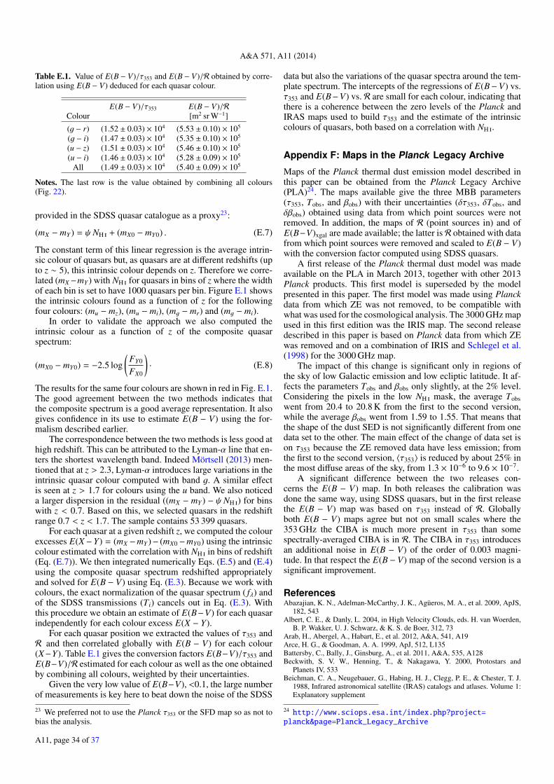
A&A 571, A11 (2014)

Table E.1. Value of E(B − V)/τ353 and E(B − V)/R obtained by corre-lation using E(B − V) deduced for each quasar colour.

E(B − V)/τ353 E(B − V)/RColour [m2 sr W−1]

(g − r) (1.52 ± 0.03) × 104 (5.53 ± 0.10) × 105

(g − i) (1.47 ± 0.03) × 104 (5.35 ± 0.10) × 105

(u − z) (1.51 ± 0.03) × 104 (5.46 ± 0.10) × 105

(u − i) (1.46 ± 0.03) × 104 (5.28 ± 0.09) × 105

All (1.49 ± 0.03) × 104 (5.40 ± 0.09) × 105

Notes. The last row is the value obtained by combining all colours(Fig. 22).

provided in the SDSS quasar catalogue as a proxy23:

(mX − mY ) = ψNH + (mX0 − mY0) . (E.7)

The constant term of this linear regression is the average intrin-sic colour of quasars but, as quasars are at different redshifts (upto z ∼ 5), this intrinsic colour depends on z. Therefore we corre-lated (mX−mY ) with NH for quasars in bins of z where the widthof each bin is set to have 1000 quasars per bin. Figure E.1 showsthe intrinsic colours found as a function of z for the followingfour colours: (mu − mz), (mu − mi), (mg − mr) and (mg − mi).

In order to validate the approach we also computed theintrinsic colour as a function of z of the composite quasarspectrum:

(mX0 − mY0) = −2.5 log(

FY0

FX0

)· (E.8)

The results for the same four colours are shown in red in Fig. E.1.The good agreement between the two methods indicates thatthe composite spectrum is a good average representation. It alsogives confidence in its use to estimate E(B − V) using the for-malism described earlier.

The correspondence between the two methods is less good athigh redshift. This can be attributed to the Lyman-α line that en-ters the shortest wavelength band. Indeed Mörtsell (2013) men-tioned that at z > 2.3, Lyman-α introduces large variations in theintrinsic quasar colour computed with band g. A similar effectis seen at z > 1.7 for colours using the u band. We also noticeda larger dispersion in the residual ((mX − mY ) − ψNH ) for binswith z < 0.7. Based on this, we selected quasars in the redshiftrange 0.7 < z < 1.7. The sample contains 53 399 quasars.

For each quasar at a given redshift z, we computed the colourexcesses E(X −Y) = (mX −mY )− (mX0 −mY0) using the intrinsiccolour estimated with the correlation with NH in bins of redshift(Eq. (E.7)). We then integrated numerically Eqs. (E.5) and (E.4)using the composite quasar spectrum redshifted appropriatelyand solved for E(B − V) using Eq. (E.3). Because we work withcolours, the exact normalization of the quasar spectrum ( fλ) andof the SDSS transmissions (Ti) cancels out in Eq. (E.3). Withthis procedure we obtain an estimate of E(B−V) for each quasarindependently for each colour excess E(X − Y).

For each quasar position we extracted the values of τ353 andR and then correlated globally with E(B − V) for each colour(X−Y). Table E.1 gives the conversion factors E(B−V)/τ353 andE(B−V)/R estimated for each colour as well as the one obtainedby combining all colours, weighted by their uncertainties.

Given the very low value of E(B−V), <0.1, the large numberof measurements is key here to beat down the noise of the SDSS

23 We preferred not to use the Planck τ353 or the SFD map so as not tobias the analysis.

data but also the variations of the quasar spectra around the tem-plate spectrum. The intercepts of the regressions of E(B−V) vs.τ353 and E(B−V) vs. R are small for each colour, indicating thatthere is a coherence between the zero levels of the Planck andIRAS maps used to build τ353 and the estimate of the intrinsiccolours of quasars, both based on a correlation with NH .

Appendix F: Maps in the Planck Legacy Archive

Maps of the Planck thermal dust emission model described inthis paper can be obtained from the Planck Legacy Archive(PLA)24. The maps available give the three MBB parameters(τ353, Tobs, and βobs) with their uncertainties (δτ353, δTobs, andδβobs) obtained using data from which point sources were notremoved. In addition, the maps of R (point sources in) and ofE(B−V)xgal are made available; the latter is R obtained with datafrom which point sources were removed and scaled to E(B − V)with the conversion factor computed using SDSS quasars.

A first release of the Planck thermal dust model was madeavailable on the PLA in March 2013, together with other 2013Planck products. This first model is superseded by the modelpresented in this paper. The first model was made using Planckdata from which ZE was not removed, to be compatible withwhat was used for the cosmological analysis. The 3000 GHz mapused in this first edition was the IRIS map. The second releasedescribed in this paper is based on Planck data from which ZEwas removed and on a combination of IRIS and Schlegel et al.(1998) for the 3000 GHz map.

The impact of this change is significant only in regions ofthe sky of low Galactic emission and low ecliptic latitude. It af-fects the parameters Tobs and βobs only slightly, at the 2% level.Considering the pixels in the low NH mask, the average Tobswent from 20.4 to 20.8 K from the first to the second version,while the average βobs went from 1.59 to 1.55. That means thatthe shape of the dust SED is not significantly different from onedata set to the other. The main effect of the change of data set ison τ353 because the ZE removed data have less emission; fromthe first to the second version, 〈τ353〉 is reduced by about 25% inthe most diffuse areas of the sky, from 1.3 × 10−6 to 9.6 × 10−7.

A significant difference between the two releases con-cerns the E(B − V) map. In both releases the calibration wasdone the same way, using SDSS quasars, but in the first releasethe E(B − V) map was based on τ353 instead of R. Globallyboth E(B − V) maps agree but not on small scales where the353 GHz the CIBA is much more present in τ353 than somespectrally-averaged CIBA is in R. The CIBA in τ353 introducesan additional noise in E(B − V) of the order of 0.003 magni-tude. In that respect the E(B− V) map of the second version is asignificant improvement.

ReferencesAbazajian, K. N., Adelman-McCarthy, J. K., Agüeros, M. A., et al. 2009, ApJS,

182, 543Albert, C. E., & Danly, L. 2004, in High Velocity Clouds, eds. H. van Woerden,

B. P. Wakker, U. J. Schwarz, & K. S. de Boer, 312, 73Arab, H., Abergel, A., Habart, E., et al. 2012, A&A, 541, A19Arce, H. G., & Goodman, A. A. 1999, ApJ, 512, L135Battersby, C., Bally, J., Ginsburg, A., et al. 2011, A&A, 535, A128Beckwith, S. V. W., Henning, T., & Nakagawa, Y. 2000, Protostars and

Planets IV, 533Beichman, C. A., Neugebauer, G., Habing, H. J., Clegg, P. E., & Chester, T. J.

1988, Infrared astronomical satellite (IRAS) catalogs and atlases. Volume 1:Explanatory supplement

24 http://www.sciops.esa.int/index.php?project=planck&page=Planck_Legacy_Archive

A11, page 34 of 37

Planck collaboration: Planck 2013 results. XI.

Bennett, C. L., Fixsen, D. J., Hinshaw, G., et al. 1994, ApJ, 434, 587Bennett, C. L., Larson, D., Weiland, J. L., et al. 2013, ApJS, 208, 20Birnstiel, T., Klahr, H., & Ercolano, B. 2012, A&A, 539, A148Blain, A. W., Barnard, V. E., & Chapman, S. C. 2003, MNRAS, 338, 733Blitz, L., Bazell, D., & Desert, F. X. 1990, ApJ, 352, L13Bohlin, R. C., Savage, B. D., & Drake, J. F. 1978, ApJ, 224, 132Bolatto, A. D., Wolfire, M., & Leroy, A. K. 2013, ARA&A, 51, 207Boulanger, F., & Pérault, M. 1988, ApJ, 330, 964Boulanger, F., Abergel, A., Bernard, J.-P., et al. 1996, A&A, 312, 256Brauer, F., Dullemond, C. P., & Henning, T. 2008, A&A, 480, 859Burstein, D., & Heiles, C. 1978, ApJ, 225, 40Calabretta, M. R., & Greisen, E. W. 2002, A&A, 395, 1077Cambrésy, L., Boulanger, F., Lagache, G., & Stepnik, B. 2001, A&A, 375, 999Cardelli, J. A., Clayton, G. C., & Mathis, J. S. 1989, ApJ, 345, 245Compiègne, M., Verstraete, L., Jones, A., et al. 2011, A&A, 525, A103Dale, D. A., Aniano, G., Engelbracht, C. W., et al. 2012, ApJ, 745, 95Delabrouille, J., Betoule, M., Melin, J.-B., et al. 2013, A&A, 553, A96Désert, F. X., Bazell, D., & Boulanger, F. 1988, ApJ, 334, 815Désert, F.-X., Macías-Pérez, J. F., Mayet, F., et al. 2008, A&A, 481, 411Draine, B. T. 2003, ARA&A, 41, 241Draine, B. T., & Li, A. 2007, ApJ, 657, 810Dupac, X., Bernard, J.-P., Boudet, N., et al. 2003, A&A, 404, L11Finkbeiner, D. P., Davis, M., & Schlegel, D. J. 1999, ApJ, 524, 867Fitzpatrick, E. L. 1999, PASP, 111, 63Fitzpatrick, E. L., & Massa, D. 2005, AJ, 130, 1127Gillmon, K., Shull, J. M., Tumlinson, J., & Danforth, C. 2006, ApJ, 636, 891Goodman, A. A., Pineda, J. E., & Schnee, S. L. 2009, ApJ, 692, 91Górski, K. M., Hivon, E., Banday, A. J., et al. 2005, ApJ, 622, 759Grenier, I. A., Casandjian, J.-M., & Terrier, R. 2005, Science, 307, 1292Heiles, C., Reach, W. T., & Koo, B.-C. 1988, ApJ, 332, 313Hildebrand, R. H. 1983, QJRAS, 24, 267Hinshaw, G., Weiland, J. L., Hill, R. S., et al. 2009, ApJS, 180, 225Jones, D. O., West, A. A., & Foster, J. B. 2011, AJ, 142, 44Juvela, M., & Ysard, N. 2012a, A&A, 541, A33Juvela, M., & Ysard, N. 2012b, A&A, 539, A71Juvela, M., Montillaud, J., Ysard, N., & Lunttila, T. 2013, A&A, 556, A63Kainulainen, J., Federrath, C., & Henning, T. 2013, A&A, 553, L8Kalberla, P. M. W., Burton, W. B., Hartmann, D., et al. 2005, A&A, 440, 775Kelly, B. C., Shetty, R., Stutz, A. M., et al. 2012, ApJ, 752, 55Kelsall, T., Weiland, J. L., Franz, B. A., et al. 1998, ApJ, 508, 44Knapp, G. R., & Kerr, F. J. 1974, A&A, 35, 361Köhler, M., Guillet, V., & Jones, A. 2011, A&A, 528, A96Köhler, M., Stepnik, B., Jones, A. P., et al. 2012, A&A, 548, A61Lagache, G., Abergel, A., Boulanger, F., Désert, F. X., & Puget, J.-L. 1999,

A&A, 344, 322Lagache, G., Haffner, L. M., Reynolds, R. J., & Tufte, S. L. 2000, A&A, 354,

247Launhardt, R., Stutz, A. M., Schmiedeke, A., et al. 2013, A&A, 551, A98Lebrun, F., Paul, J. A., Bignami, G. F., et al. 1982, A&A, 107, 390Lilley, A. E. 1955, ApJ, 121, 559Liszt, H. 2014, ApJ, 780, 10Lockman, F. J., & Condon, J. J. 2005, AJ, 129, 1968Lombardi, M., Alves, J., & Lada, C. J. 2011, A&A, 535, A16Markwardt, C. B. 2009, in Astronomical Data Analysis Software and Systems

XVIII, eds. D. A. Bohlender, D. Durand, & P. Dowler, 411, 251Martin, P. G., Roy, A., Bontemps, S., et al. 2012, ApJ, 751, 28Mathis, J. S., Rumpl, W., & Nordsieck, K. H. 1977, ApJ, 217, 425Mathis, J. S., Mezger, P. G., & Panagia, N. 1983, A&A, 128, 212McClure-Griffiths, N. M., Pisano, D. J., Calabretta, M. R., et al. 2009, ApJS,

181, 398Meny, C., Gromov, V., Boudet, N., et al. 2007, A&A, 468, 171Miville-Deschênes, M. 2011, in ASP Conf. Ser. 449, eds. P. Bastien, N. Manset,

D. P. Clemens, & N. St-Louis, 187Miville-Deschênes, M.-A., & Lagache, G. 2005, ApJS, 157, 302Miville-Deschênes, M.-A., Lagache, G., Boulanger, F., & Puget, J.-L. 2007,

A&A, 469, 595Mörtsell, E. 2013, A&A, 550, A80Moshir, M., Kopman, G., & Conrow, T. A. O. 1992, IRAS Faint Source Survey,

Explanatory supplement version 2O’Donnell, J. E. 1994, ApJ, 422, 158Ormel, C. W., Min, M., Tielens, A. G. G. M., Dominik, C., & Paszun, D. 2011,

A&A, 532, A43Ossenkopf, V., & Henning, T. 1994, A&A, 291, 943Paradis, D., Veneziani, M., Noriega-Crespo, A., et al. 2010, A&A, 520, L8Paradis, D., Paladini, R., Noriega-Crespo, A., et al. 2012, A&A, 537, A113Peek, J. E. G., & Graves, G. J. 2010, ApJ, 719, 415Pénin, A., Lagache, G., Noriega-Crespo, A., et al. 2012, A&A, 543, A123Peretto, N., André, P., Könyves, V., et al. 2012, A&A, 541, A63

Pineda, J. E., Caselli, P., & Goodman, A. A. 2008, ApJ, 679, 481Planck Collaboration VII. 2011, A&A, 536, A7Planck Collaboration XVII. 2011, A&A, 536, A17Planck Collaboration XVIII. 2011, A&A, 536, A18Planck Collaboration XIX. 2011, A&A, 536, A19Planck Collaboration XXI. 2011, A&A, 536, A21Planck Collaboration XXIII. 2011, A&A, 536, A23Planck Collaboration XXIV. 2011, A&A, 536, A24Planck Collaboration XXV. 2011, A&A, 536, A25Planck Collaboration I. 2014, A&A, 571, A1Planck Collaboration II. 2014, A&A, 571, A2Planck Collaboration III. 2014, A&A, 571, A3Planck Collaboration IV. 2014, A&A, 571, A4Planck Collaboration V. 2014, A&A, 571, A5Planck Collaboration VI. 2014, A&A, 571, A6Planck Collaboration VII. 2014, A&A, 571, A7Planck Collaboration VIII. 2014, A&A, 571, A8Planck Collaboration IX. 2014, A&A, 571, A9Planck Collaboration X. 2014, A&A, 571, A10Planck Collaboration XI. 2014, A&A, 571, A11Planck Collaboration XII. 2014, A&A, 571, A12Planck Collaboration XIII. 2014, A&A, 571, A13Planck Collaboration XIV. 2014, A&A, 571, A14Planck Collaboration XV. 2014, A&A, 571, A15Planck Collaboration XVI. 2014, A&A, 571, A16Planck Collaboration XVII. 2014, A&A, 571, A17Planck Collaboration XVIII. 2014, A&A, 571, A18Planck Collaboration XIX. 2014, A&A, 571, A19Planck Collaboration XX. 2014, A&A, 571, A20Planck Collaboration XXI. 2014, A&A, 571, A21Planck Collaboration XXII. 2014, A&A, 571, A22Planck Collaboration XXIII. 2014, A&A, 571, A23Planck Collaboration XXIV. 2014, A&A, 571, A24Planck Collaboration XXV. 2014, A&A, 571, A25Planck Collaboration XXVI. 2014, A&A, 571, A26Planck Collaboration XXVII. 2014, A&A, 571, A27Planck Collaboration XXVIII. 2014, A&A, 571, A28Planck Collaboration XXIX. 2014, A&A, 571, A29Planck Collaboration XXX. 2014, A&A, 571, A30Planck Collaboration XXXI. 2014, A&A, 571, A31Planck Collaboration Int. XIV. 2014, A&A, 564, A45Planck Collaboration Int. XVII. 2014, A&A, 566, A55Puget, J.-L., Abergel, A., Bernard, J.-P., et al. 1996, A&A, 308, L5Rachford, B. L., Snow, T. P., Tumlinson, J., et al. 2002, ApJ, 577, 221Rachford, B. L., Snow, T. P., Destree, J. D., et al. 2009, ApJS, 180, 125Reach, W. T., Koo, B.-C., & Heiles, C. 1994, ApJ, 429, 672Reach, W. T., Wall, W. F., & Odegard, N. 1998, ApJ, 507, 507Roy, A., Martin, P. G., Polychroni, D., et al. 2013, ApJ, 763, 55Ryter, C., Cesarsky, C. J., & Audouze, J. 1975, ApJ, 198, 103Savage, B. D., & Jenkins, E. B. 1972, ApJ, 172, 491Schlafly, E. F., & Finkbeiner, D. P. 2011, ApJ, 737, 103Schlafly, E. F., Finkbeiner, D. P., Schlegel, D. J., et al. 2010, ApJ, 725, 1175Schlegel, D. J., Finkbeiner, D. P., & Davis, M. 1998, ApJ, 500, 525 (SFD)Schnee, S., Kauffmann, J., Goodman, A., & Bertoldi, F. 2007, ApJ, 657, 838Schnee, S., Li, J., Goodman, A. A., & Sargent, A. I. 2008, ApJ, 684, 1228Schneider, D. P., Richards, G. T., Hall, P. B., et al. 2010, AJ, 139, 2360Schneider, N., Bontemps, S., Simon, R., et al. 2011, A&A, 529, A1Shetty, R., Kauffmann, J., Schnee, S., & Goodman, A. A. 2009a, ApJ, 696, 676Shetty, R., Kauffmann, J., Schnee, S., Goodman, A. A., & Ercolano, B. 2009b,

ApJ, 696, 2234Skrutskie, M. F., Cutri, R. M., Stiening, R., et al. 2006, AJ, 131, 1163Stepnik, B., Abergel, A., Bernard, J.-P., et al. 2003, A&A, 398, 551Vanden Berk, D. E., Richards, G. T., Bauer, A., et al. 2001, AJ, 122, 549Veneziani, M., Ade, P. A. R., Bock, J. J., et al. 2010, ApJ, 713, 959Veneziani, M., Piacentini, F., Noriega-Crespo, A., et al. 2013, ApJ, 772, 56Wakker, B. P. 2006, ApJS, 163, 282Weingartner, J. C., & Draine, B. T. 2001, ApJ, 548, 296Ysard, N., Juvela, M., Demyk, K., et al. 2012, A&A, 542, A21

1 APC, AstroParticule et Cosmologie, Université Paris Diderot,CNRS/IN2P3, CEA/lrfu, Observatoire de Paris, Sorbonne ParisCité, 10 rue Alice Domon et Léonie Duquet, 75205 Paris Cedex13, France

2 Aalto University Metsähovi Radio Observatory and Dept of RadioScience and Engineering, PO Box 13000, 00076 AALTO, Finland

A11, page 35 of 37

A&A 571, A11 (2014)

3 African Institute for Mathematical Sciences, 6-8 Melrose Road,Muizenberg, Cape Town, South Africa

4 Agenzia Spaziale Italiana Science Data Center, via del Politecnicosnc, 00133 Roma, Italy

5 Agenzia Spaziale Italiana, Viale Liegi 26, Roma, Italy6 Astrophysics Group, Cavendish Laboratory, University of

Cambridge, J J Thomson Avenue, Cambridge CB3 0HE, UK7 Astrophysics & Cosmology Research Unit, School of Mathematics,

Statistics & Computer Science, University of KwaZulu-Natal,Westville Campus, Private Bag X54001, 4000 Durban, South Africa

8 CITA, University of Toronto, 60 St. George St., Toronto, ON M5S3H8, Canada

9 CNRS, IRAP, 9 Av. colonel Roche, BP 44346, 31028 ToulouseCedex 4, France

10 California Institute of Technology, Pasadena, California, USA11 Centre for Theoretical Cosmology, DAMTP, University of

Cambridge, Wilberforce Road, Cambridge CB3 0WA, UK12 Centro de Estudios de Física del Cosmos de Aragón (CEFCA),

Plaza San Juan 1, planta 2, 44001 Teruel, Spain13 Computational Cosmology Center, Lawrence Berkeley National

Laboratory, Berkeley, California, USA14 Consejo Superior de Investigaciones Científicas (CSIC), Madrid,

Spain15 DSM/Irfu/SPP, CEA-Saclay, 91191 Gif-sur-Yvette Cedex, France16 DTU Space, National Space Institute, Technical University of

Denmark, Elektrovej 327, 2800 Kgs. Lyngby, Denmark17 Département de Physique Théorique, Université de Genève, 24 Quai

E. Ansermet, 1211 Genève 4, Switzerland18 Département de physique, de génie physique et d’optique,

Université Laval, Québec, Canada19 Departamento de Física Fundamental, Facultad de Ciencias,

Universidad de Salamanca, 37008 Salamanca, Spain20 Departamento de Física, Universidad de Oviedo, Avda. Calvo Sotelo

s/n, Oviedo, Spain21 Department of Astronomy and Astrophysics, University of Toronto,

50 Saint George Street, Toronto, Ontario, Canada22 Department of Astrophysics/IMAPP, Radboud University

Nijmegen, PO Box 9010, 6500 GL Nijmegen, The Netherlands23 Department of Electrical Engineering and Computer Sciences,

University of California, Berkeley, California, USA24 Department of Physics & Astronomy, University of British

Columbia, 6224 Agricultural Road, Vancouver, British Columbia,Canada

25 Department of Physics and Astronomy, Dana and David DornsifeCollege of Letter, Arts and Sciences, University of SouthernCalifornia, Los Angeles, CA 90089, USA

26 Department of Physics and Astronomy, University College London,London WC1E 6BT, UK

27 Department of Physics, Florida State University, Keen PhysicsBuilding, 77 Chieftan Way, Tallahassee, Florida, USA

28 Department of Physics, Gustaf Hällströmin katu 2a, University ofHelsinki, Helsinki, Finland

29 Department of Physics, Princeton University, Princeton, New Jersey,USA

30 Department of Physics, University of California, One ShieldsAvenue, Davis, California, USA

31 Department of Physics, University of California, Santa Barbara,California, USA

32 Department of Physics, University of Illinois at Urbana-Champaign,1110 West Green Street, Urbana, Illinois, USA

33 Dipartimento di Fisica e Astronomia G. Galilei, Università degliStudi di Padova, via Marzolo 8, 35131 Padova, Italy

34 Dipartimento di Fisica e Scienze della Terra, Università di Ferrara,via Saragat 1, 44122 Ferrara, Italy

35 Dipartimento di Fisica, Università La Sapienza, P.le A. Moro 2,Roma, Italy

36 Dipartimento di Fisica, Università degli Studi di Milano, via Celoria,16, Milano, Italy

37 Dipartimento di Fisica, Università degli Studi di Trieste, via A.Valerio 2, Trieste, Italy

38 Dipartimento di Fisica, Università di Roma Tor Vergata, via dellaRicerca Scientifica 1, Roma, Italy

39 Discovery Center, Niels Bohr Institute, Blegdamsvej 17,Copenhagen, Denmark

40 Dpto. Astrofísica, Universidad de La Laguna (ULL), 38206La Laguna, Tenerife, Spain

41 European Space Agency, ESAC, Planck Science Office, Caminobajo del Castillo, s/n, Urbanización Villafranca del Castillo,Villanueva de la Cañada, Madrid, Spain

42 European Space Agency, ESTEC, Keplerlaan 1, 2201 AZNoordwijk, The Netherlands

43 Finnish Centre for Astronomy with ESO (FINCA), University ofTurku, Väisäläntie 20, 21500 Piikkiö, Finland

44 Helsinki Institute of Physics, Gustaf Hällströmin katu 2, Universityof Helsinki, Helsinki, Finland

45 INAF–Osservatorio Astrofisico di Catania, via S. Sofia 78, Catania,Italy

46 INAF–Osservatorio Astronomico di Padova, Vicolo dell’Osservatorio 5, Padova, Italy

47 INAF–Osservatorio Astronomico di Roma, via di Frascati 33,Monte Porzio Catone, Italy

48 INAF–Osservatorio Astronomico di Trieste, via G.B. Tiepolo 11,Trieste, Italy

49 INAF Istituto di Radioastronomia, via P. Gobetti 101, 40129Bologna, Italy

50 INAF/IASF Bologna, via Gobetti 101, Bologna, Italy51 INAF/IASF Milano, via E. Bassini 15, Milano, Italy52 INFN, Sezione di Bologna, via Irnerio 46, 40126, Bologna, Italy53 INFN, Sezione di Roma 1, Università di Roma Sapienza, Piazzale

Aldo Moro 2, 00185, Roma, Italy54 INFN/National Institute for Nuclear Physics, via Valerio 2, 34127

Trieste, Italy55 IPAG: Institut de Planétologie et d’Astrophysique de Grenoble,

Université Joseph Fourier, Grenoble 1 / CNRS-INSU, UMR 5274,38041 Grenoble, France

56 ISDC Data Centre for Astrophysics, University of Geneva, ch.d’Ecogia 16, Versoix, Switzerland

57 IUCAA, Post Bag 4, Ganeshkhind, Pune University Campus,411 007 Pune, India

58 Imperial College London, Astrophysics group, Blackett Laboratory,Prince Consort Road, London, SW7 2AZ, UK

59 Infrared Processing and Analysis Center, California Institute ofTechnology, Pasadena, CA 91125, USA

60 Institut Néel, CNRS, Université Joseph Fourier Grenoble I, 25 ruedes Martyrs, Grenoble, France

61 Institut Universitaire de France, 103 Bd Saint-Michel, 75005, Paris,France

62 Institut d’Astrophysique Spatiale, CNRS (UMR8617) UniversitéParis-Sud 11, Bâtiment 121, Orsay, France

63 Institut d’Astrophysique de Paris, CNRS (UMR7095), 98bis BdArago, 75014 Paris, France

64 Institute for Space Sciences, Bucharest-Magurale, Romania65 Institute of Astronomy and Astrophysics, Academia Sinica, Taipei,

Taiwan66 Institute of Astronomy, University of Cambridge, Madingley Road,

Cambridge CB3 0HA, UK67 Institute of Theoretical Astrophysics, University of Oslo, Blindern,

Oslo, Norway68 Instituto de Astrofísica de Canarias, C/Vía Láctea s/n, La Laguna,

Tenerife, Spain69 Instituto de Física de Cantabria (CSIC-Universidad de Cantabria),

Avda. de los Castros s/n, Santander, Spain70 Jet Propulsion Laboratory, California Institute of Technology, 4800

Oak Grove Drive, Pasadena, California, USA71 Jodrell Bank Centre for Astrophysics, Alan Turing Building, School

of Physics and Astronomy, The University of Manchester, OxfordRoad, Manchester, M13 9PL, UK

72 Kavli Institute for Cosmology Cambridge, Madingley Road,Cambridge, CB3 0HA, UK

73 LAL, Université Paris-Sud, CNRS/IN2P3, Orsay, France

A11, page 36 of 37

Planck collaboration: Planck 2013 results. XI.

74 LERMA, CNRS, Observatoire de Paris, 61 Avenue del’Observatoire, Paris, France

75 Laboratoire AIM, IRFU/Service d’Astrophysique – CEA/DSM –CNRS – Université Paris Diderot, Bât. 709, CEA-Saclay, 91191 Gif-sur-Yvette Cedex, France

76 Laboratoire Traitement et Communication de l’Information, CNRS(UMR 5141) and Télécom ParisTech, 46 rue Barrault, 75634 ParisCedex 13, France

77 Laboratoire de Physique Subatomique et de Cosmologie, UniversitéJoseph Fourier Grenoble I, CNRS/IN2P3, Institut NationalPolytechnique de Grenoble, 53 rue des Martyrs, 38026 GrenobleCedex, France

78 Laboratoire de Physique Théorique, Université Paris-Sud 11 &CNRS, Bâtiment 210, 91405 Orsay, France

79 Lawrence Berkeley National Laboratory, Berkeley, California, USA80 Max-Planck-Institut für Astrophysik, Karl-Schwarzschild-Str. 1,

85741 Garching, Germany81 McGill Physics, Ernest Rutherford Physics Building, McGill

University, 3600 rue University, Montréal, QC, H3A 2T8, Canada82 MilliLab, VTT Technical Research Centre of Finland, Tietotie 3,

Espoo, Finland83 National University of Ireland, Department of Experimental

Physics, Maynooth, Co. Kildare, Ireland84 Niels Bohr Institute, Blegdamsvej 17, Copenhagen, Denmark85 Observational Cosmology, Mail Stop 367-17, California Institute of

Technology, Pasadena, CA, 91125, USA86 Optical Science Laboratory, University College London, Gower

Street, London, UK

87 Princeton University Observatory, Peyton Hall, Princeton, NJ08544-1001, USA

88 SB-ITP-LPPC, EPFL, 1015, Lausanne, Switzerland89 SISSA, Astrophysics Sector, via Bonomea 265, 34136 Trieste, Italy90 School of Physics and Astronomy, Cardiff University, Queens

Buildings, The Parade, Cardiff, CF24 3AA, UK91 Space Research Institute (IKI), Russian Academy of Sciences,

Profsoyuznaya Str, 84/32, 117997 Moscow, Russia92 Space Sciences Laboratory, University of California, Berkeley,

California, USA93 Special Astrophysical Observatory, Russian Academy of Sciences,

Nizhnij Arkhyz, Zelenchukskiy region, 369167 Karachai-Cherkessian Republic, Russia

94 Stanford University, Dept of Physics, Varian Physics Bldg, 382 viaPueblo Mall, Stanford, California, USA

95 Sub-Department of Astrophysics, University of Oxford, KebleRoad, Oxford OX1 3RH, UK

96 Theory Division, PH-TH, CERN, 1211 Geneva 23, Switzerland97 UPMC Univ. Paris 06, UMR7095, 98bis Boulevard Arago, 75014

Paris, France98 Université de Toulouse, UPS-OMP, IRAP, 31028 Toulouse Cedex 4,

France99 Universities Space Research Association, Stratospheric Observatory

for Infrared Astronomy, MS 232-11, Moffett Field, CA 94035, USA100 University of Granada, Departamento de Física Teórica y del

Cosmos, Facultad de Ciencias, Granada, Spain101 Warsaw University Observatory, Aleje Ujazdowskie 4, 00-478

Warszawa, Poland

A11, page 37 of 37