Pitching-Flapping Wings - UC Irvine

UC IrvineUC Irvine Electronic Theses and Dissertations

TitleNumerical and Analytical Investigation of the Unsteady Lift Characteristics of Plunging-Pitching-Flapping Wings

Permalinkhttps://escholarship.org/uc/item/6z5194xk

AuthorMuoio, Ryan

Publication Date2016 Peer reviewed|Thesis/dissertation

eScholarship.org Powered by the California Digital LibraryUniversity of California

UNIVERSITY OF CALIFORNIA,IRVINE

Numerical and Analytical Investigation of the Unsteady LiftCharacteristics of Plunging-Pitching-Flapping Wings

THESIS

submitted in partial satisfaction of the requirementsfor the degree of

MASTER OF SCIENCE

in Mechanical and Aerospace Engineering

by

Ryan Muoio

Thesis Committee:Professor Haithem Taha, Chair

Professor Kenneth MeaseProfessor Solmaz Kia

2016

© 2016 Ryan Muoio

DEDICATION

To:

The One who created me with: 1) enough determination to make it this far, and 2) thespark of lunacy to want to go even further in academia.

My mother, who supported me financially during my undergraduate career and who hasalways been there to offer me help when needed.

My father, who built me up with words of encouragement, always believing in me, evenwhen I didn’t believe in myself.

My friends, who always thought me to be smarter than I am; if it weren’t for you, Iwouldn’t have pushed myself to try to attain the level of knowledge you thought I already

had.

ii

TABLE OF CONTENTS

Page

LIST OF FIGURES v

ACKNOWLEDGMENTS vii

CURRICULUM VITAE viii

ABSTRACT OF THE THESIS ix

1 Introduction 1

2 Theodorsen 32.1 Velocity Potentials . . . . . . . . . . . . . . . . . . . . . . . . . . . . . . . . 32.2 Induced Loads . . . . . . . . . . . . . . . . . . . . . . . . . . . . . . . . . . . 6

3 Leishman 113.1 State-Space Representation . . . . . . . . . . . . . . . . . . . . . . . . . . . 11

4 Garrick 14

5 Unsteady Vortex Lattice Method (UVLM) 175.1 Biot-Savart: Function . . . . . . . . . . . . . . . . . . . . . . . . . . . . . . . 185.2 Geometry . . . . . . . . . . . . . . . . . . . . . . . . . . . . . . . . . . . . . 21

5.2.1 Time-Invariant Geometry: Lines 99-108 . . . . . . . . . . . . . . . . . 215.2.2 Time-Varying Geometry: Lines 134-148 . . . . . . . . . . . . . . . . . 23

5.3 Kinematics: Lines 114-142 . . . . . . . . . . . . . . . . . . . . . . . . . . . . 245.4 Influence Coefficient Matrix (ICM): Lines 150-160 . . . . . . . . . . . . . . . 265.5 Right Hand Side: Lines 163-179 . . . . . . . . . . . . . . . . . . . . . . . . . 305.6 Solving the System: Lines 182-234 . . . . . . . . . . . . . . . . . . . . . . . . 32

5.6.1 Pressure Coefficient Cp . . . . . . . . . . . . . . . . . . . . . . . . . . 335.6.2 Lift Coefficient CL . . . . . . . . . . . . . . . . . . . . . . . . . . . . 37

5.7 Convection: Lines 237-270 . . . . . . . . . . . . . . . . . . . . . . . . . . . . 38

6 Results 446.1 Verification . . . . . . . . . . . . . . . . . . . . . . . . . . . . . . . . . . . . 446.2 Lift Shape Validation . . . . . . . . . . . . . . . . . . . . . . . . . . . . . . . 46

6.2.1 Plunging . . . . . . . . . . . . . . . . . . . . . . . . . . . . . . . . . . 47

iii

6.2.2 Pitching . . . . . . . . . . . . . . . . . . . . . . . . . . . . . . . . . . 536.2.3 Flapping . . . . . . . . . . . . . . . . . . . . . . . . . . . . . . . . . . 58

6.3 Root-Mean Square Error . . . . . . . . . . . . . . . . . . . . . . . . . . . . . 636.4 Phase Difference . . . . . . . . . . . . . . . . . . . . . . . . . . . . . . . . . 656.5 Lift Amplitude . . . . . . . . . . . . . . . . . . . . . . . . . . . . . . . . . . 686.6 Mean Lift . . . . . . . . . . . . . . . . . . . . . . . . . . . . . . . . . . . . . 71

7 Conclusion and Future Work 767.1 Conclusion . . . . . . . . . . . . . . . . . . . . . . . . . . . . . . . . . . . . . 767.2 Future Work . . . . . . . . . . . . . . . . . . . . . . . . . . . . . . . . . . . . 77

7.2.1 Two-Dimensional . . . . . . . . . . . . . . . . . . . . . . . . . . . . . 777.2.2 Three-Dimensional . . . . . . . . . . . . . . . . . . . . . . . . . . . . 78

.1 Appendix A . . . . . . . . . . . . . . . . . . . . . . . . . . . . . . . . . . . . 80.1.1 Geometric Constants . . . . . . . . . . . . . . . . . . . . . . . . . . . 80

.2 Appendix B . . . . . . . . . . . . . . . . . . . . . . . . . . . . . . . . . . . . 80.2.1 Unsteady Vortex Lattice Method Code . . . . . . . . . . . . . . . . . 80.2.2 Theodorsen Code . . . . . . . . . . . . . . . . . . . . . . . . . . . . . 91.2.3 Leishman Code . . . . . . . . . . . . . . . . . . . . . . . . . . . . . . 93.2.4 Phase Difference Code . . . . . . . . . . . . . . . . . . . . . . . . . . 95

iv

LIST OF FIGURES

Page

2.1 Conformal representation of the wing profile by a circle. . . . . . . . . . . . . 42.2 Parameters of the airfoil-flap combination. . . . . . . . . . . . . . . . . . . . 52.3 Conformal representation with circulatory flow. . . . . . . . . . . . . . . . . 8

5.1 Coordinate system for UVLM approach. . . . . . . . . . . . . . . . . . . . . 185.2 Pictorial representation of the Biot-Savart law. . . . . . . . . . . . . . . . . . 195.3 A look at the Rankine vortex model. . . . . . . . . . . . . . . . . . . . . . . 205.4 Discretization of the airfoil using collocation points. . . . . . . . . . . . . . . 22

6.1 Lift coefficient versus time. . . . . . . . . . . . . . . . . . . . . . . . . . . . . 466.2 A 2D visualization of an oscillating flap deflection. The black is the flat plate

with a flap; the cyan is the wake convection. This image is from the UVLMmid-run. . . . . . . . . . . . . . . . . . . . . . . . . . . . . . . . . . . . . . . 47

6.3 Plunging for k = 0.01. . . . . . . . . . . . . . . . . . . . . . . . . . . . . . . 486.4 Plunging for k = 0.2. . . . . . . . . . . . . . . . . . . . . . . . . . . . . . . . 496.5 Plunging for k = 0.4. . . . . . . . . . . . . . . . . . . . . . . . . . . . . . . . 506.6 Plunging for k = 0.6. . . . . . . . . . . . . . . . . . . . . . . . . . . . . . . . 516.7 Zoomed in case of plunging at k = 0.01 to show erroneous results of Leishman’s

formulation. . . . . . . . . . . . . . . . . . . . . . . . . . . . . . . . . . . . . 526.8 Pitching for k = 0.01. . . . . . . . . . . . . . . . . . . . . . . . . . . . . . . . 546.9 Pitching for k = 0.2. . . . . . . . . . . . . . . . . . . . . . . . . . . . . . . . 556.10 Pitching for k = 0.4. . . . . . . . . . . . . . . . . . . . . . . . . . . . . . . . 566.11 Pitching for k = 0.6. . . . . . . . . . . . . . . . . . . . . . . . . . . . . . . . 576.12 Flapping for k = 0.01. . . . . . . . . . . . . . . . . . . . . . . . . . . . . . . 596.13 Flapping for k = 0.2. . . . . . . . . . . . . . . . . . . . . . . . . . . . . . . . 606.14 Flapping for k = 0.4. . . . . . . . . . . . . . . . . . . . . . . . . . . . . . . . 616.15 Flapping for k = 0.6. . . . . . . . . . . . . . . . . . . . . . . . . . . . . . . . 626.16 RMSe trend for plunging, pitching, and flapping. . . . . . . . . . . . . . . . . 646.17 The phase difference φ for a plunging motion. . . . . . . . . . . . . . . . . . 656.18 The phase difference φ for a pitching motion. . . . . . . . . . . . . . . . . . . 666.19 The phase difference φ for a flapping motion. . . . . . . . . . . . . . . . . . . 676.20 The lift amplitude for a plunging motion. . . . . . . . . . . . . . . . . . . . . 686.21 The lift amplitude for a pitching motion. . . . . . . . . . . . . . . . . . . . . 696.22 The lift amplitude for a flapping motion. . . . . . . . . . . . . . . . . . . . . 706.23 The mean lift for plunging at varying frequency. . . . . . . . . . . . . . . . . 72

v

6.24 The mean lift for pitching at varying frequency. . . . . . . . . . . . . . . . . 736.25 The mean lift for flapping at varying frequency. . . . . . . . . . . . . . . . . 74

7.1 Visualization of 3D UVLM code with a flap deflection. There are four chord-wise panels and fourteen spanwise panels. The chord length is one meter andthe span length is six meters. . . . . . . . . . . . . . . . . . . . . . . . . . . 79

vi

ACKNOWLEDGMENTS

I would like to extend my thanks to the Department of Mechanical and Aerospace Engineer-ing for granting me a Teaching Assitantship for final two quarters of my master’s program.Without the financial support, I wouldn’t have been able to complete this degree.

Professor Taha, without your patient guidance of my academic path, I doubt I would bewhere I am today. You accepted me as you student even though I had no experience inyour area of expertise. You subsequently spent hours teaching me; and I spent hours notgrasping the information as quickly as others may have, yet you continued to pour time intome. Your tutelage has inspired me to become great, both as a person and a teacher.

Friends, yes, I’m grateful to say I have many. To those in school with me, who brainstormedwith me, showed me I was wrong, and taught me how to be right, you know who you are. Butbecause I said I would, I’ll name a few: Meng-Ting, Edgar, Tuan, James, Zeinab, Quentin,Vatche, and Joseph. You’ve helped me more than you know.

vii

CURRICULUM VITAE

Ryan Muoio

EDUCATION

Master of Science in Mechanical and Aerospace 2016University of California, Irvine Irvine, California

Bachelor of Science in Physics 2012University of California, Riverside Riverside, California

RESEARCH EXPERIENCE

Graduate Researcher 2015–2016University of California, Irvine Irvine, California

TEACHING EXPERIENCE

Teaching Assistant 2016UCI Classes: Mechanical Vibrations and Mechanical Lab Irvine, California

High School Tutor 2014Freelance for AP Physics students Newport, California

WORK EXPERIENCE

Component Engineer 2012–2014Extron Electronics Anaheim, California

Research Engineer 2016University of California, Irvine Irvine, California

viii

ABSTRACT OF THESIS

Numerical and Analytical Investigation of the Unsteady LiftCharacteristics of Plunging-Pitching-Flapping Wings

By

Ryan Muoio

Master of Science in Mechanical and Aerospace Engineering

University of California, Irvine, 2016

Professor Haithem Taha, Chair

Three methods for computing the unsteady lift response due to basic kinematic motion—

plunging, pitching, and flapping—are compared. The first two methods are analytical models

developed by Theodorsen and Leishman, while the third method is a numerical method

known as the unsteady vortex lattice method. The MATLAB code for this numerical method

is included. All calculations are evaluated for the potential flow case.

ix

Chapter 1

Introduction

The lift response due to a oscillating flap deflection has been a topic of research since the

1930s, with it first being addressed for the harmonic case by Theodorsen in 1935 [1]. Restrict-

ing the theory to potential flow and the Kutta condition, Theodorsen resolved the solution

of the problem into Bessel functions of the first and second kind and of zero and first order.

Two year later, in 1937, Garrick [2] extended Theodorsen’s theory to include the horizontal

force due to flap deflection. He used as a starting point the work of Wagner [3], then applied

the compact methods outlined by von Karman and Burgers [4] to treat the propulsion of an

airfoil oscillating in three degrees of freedom. In doing so, Garrick developed a method to

find the suction force, which can be used in both lift and drag calculations.

Skipping forward many decades, in 1994, Leishman [5] addressed the problem of unsteady lift

produced by an oscillating flap, but he described the response using step concepts. Instead of

taking into account solely harmonic motions like Theodorsen, Leishman considered the effect

of non-uniform flow, much like that of von Karman and Sears [6], R.T. Jones [7], and Wagner.

Using the Duhamel superposition integral and an improved exponential approximation to

Wagner’s step lift function, Leishman obtained a controllable canonical form of the solution.

1

With analytical tools already developed, a numerical approach known as the unsteady vortex

lattice method (UVLM) is used by the author to obtain results comparable to Theodorsen

and Leishman for induced lift. The objective of this paper is to compare the UVLM to these

two analytical lift-predicting methods.

The general motivation for this task is to better understand the difference between select

analytical and numerical methods. It is desired to determine where and when this par-

ticular numerical approach can be used in place of the known analytical approaches, since

Theodorsen’s and Leishman’s formulations are limited to rigid bodies, whereas the UVLM

is not.

2

Chapter 2

Theodorsen

Theodore Theodorsen is considered a pioneer of classical unsteady aerodynamics, with many

published works in the field. His paper including flap deflection [1] is referenced here.

Assumptions intrinsic to the classical model are that linearized partial differential equations

and linear boundary conditions govern the problem, with loads calculated on a thin, rigid

airfoil.

2.1 Velocity Potentials

Theodorsen begins his process by determining the velocity potentials created by the position

and velocity of the individual parts in the whole of the airfoil system. The airfoil is first

represented by a circle in the ξ-plane, such that ξ = χ+ iη. A source 2Q is placed at (χ1, η1)

and a negative source −2Q at (χ1,−η1), as shown in Figure 2.1.

3

Figure 2.1: Conformal representation of the wing profile by a circle.

The flow around the circle is therefore

ϕ =Q

2πln

(χ− χ1)2 + (η − η1)2

(χ− χ1)2 + (η + η1)2

Knowing that |ξ| =√χ2 + η2 = b, the above equation is reduced to a function of one

variable.

ϕ =Q

2πln

(χ− χ1)2 + (√b2 − χ2 −

√b2 − χ2

1)2

(χ− χ1)2 + (√b2 − χ2 +

√b2 − χ2

1)2

Using the Joukowski transformation

z =ξ

2+b2

2ξ(2.1)

the function ϕ on the circle gives directly the surface potential of the chord, the projection

of the circle on the horizontal diameter in the physical plane. This transformation allows

the velocity potentials for the multiple parts of the airfoil-flap combination to be treated as

4

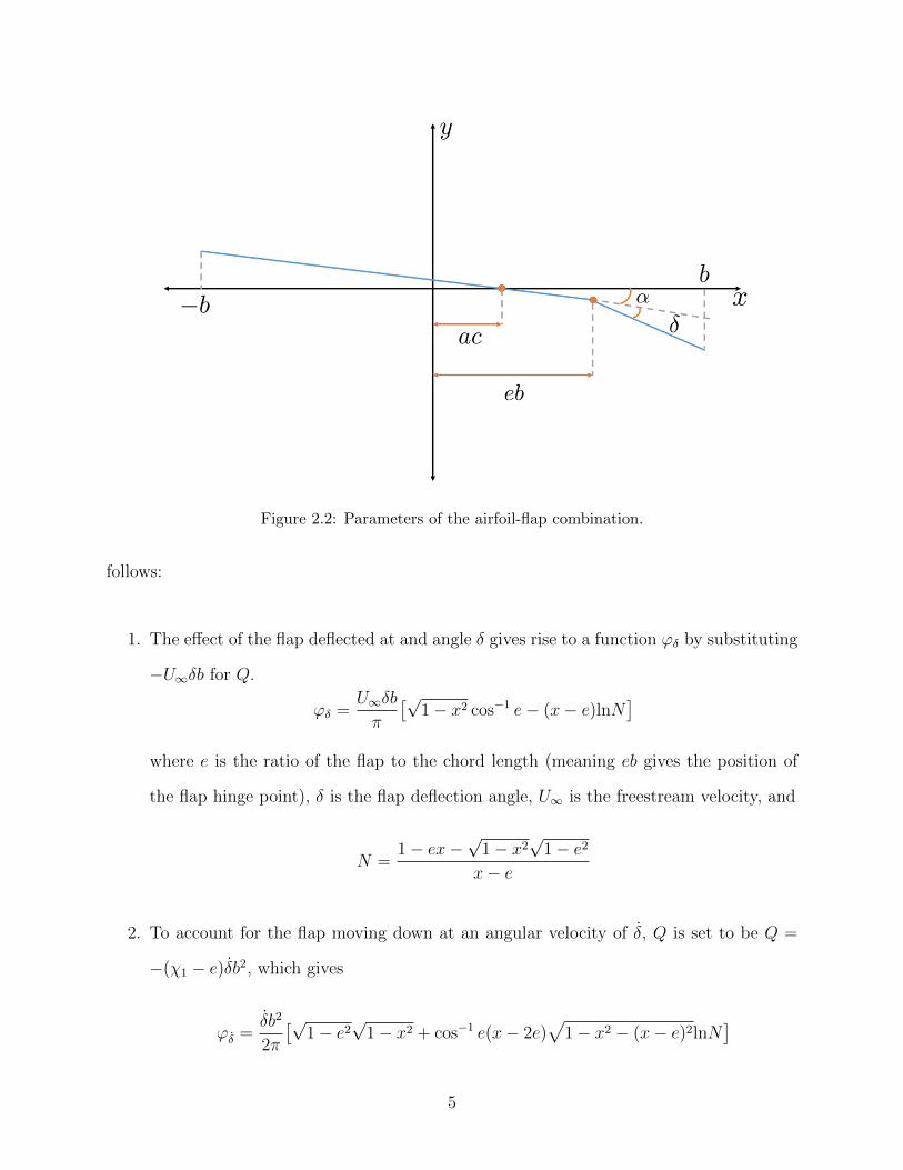
Figure 2.2: Parameters of the airfoil-flap combination.

follows:

1. The effect of the flap deflected at and angle δ gives rise to a function ϕδ by substituting

−U∞δb for Q.

ϕδ =U∞δb

π

[√1− x2 cos−1 e− (x− e)lnN

]where e is the ratio of the flap to the chord length (meaning eb gives the position of

the flap hinge point), δ is the flap deflection angle, U∞ is the freestream velocity, and

N =1− ex−

√1− x2

√1− e2

x− e

2. To account for the flap moving down at an angular velocity of δ, Q is set to be Q =

−(χ1 − e)δb2, which gives

ϕδ =δb2

2π

[√1− e2

√1− x2 + cos−1 e(x− 2e)

√1− x2 − (x− e)2lnN

]

5

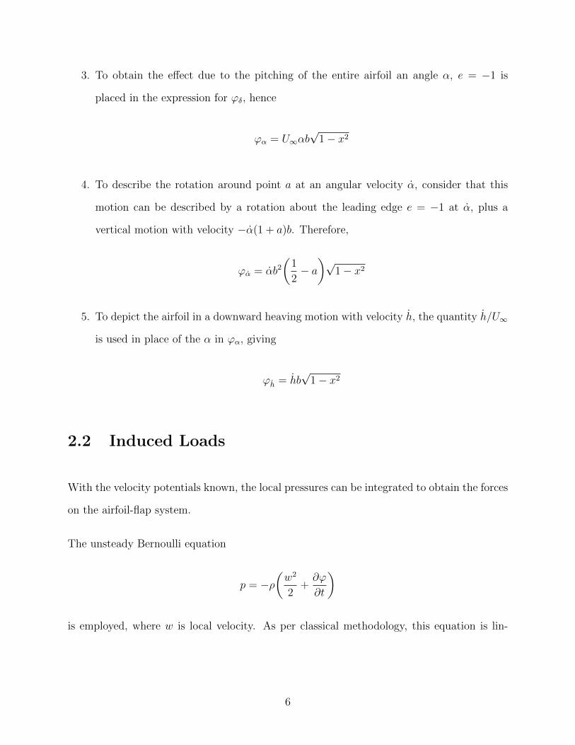
3. To obtain the effect due to the pitching of the entire airfoil an angle α, e = −1 is

placed in the expression for ϕδ, hence

ϕα = U∞αb√

1− x2

4. To describe the rotation around point a at an angular velocity α, consider that this

motion can be described by a rotation about the leading edge e = −1 at α, plus a

vertical motion with velocity −α(1 + a)b. Therefore,

ϕα = αb2

(1

2− a)√

1− x2

5. To depict the airfoil in a downward heaving motion with velocity h, the quantity h/U∞

is used in place of the α in ϕα, giving

ϕh = hb√

1− x2

2.2 Induced Loads

With the velocity potentials known, the local pressures can be integrated to obtain the forces

on the airfoil-flap system.

The unsteady Bernoulli equation

p = −ρ(w2

2+∂ϕ

∂t

)

is employed, where w is local velocity. As per classical methodology, this equation is lin-

6

earized by setting w = U∞ + ∂ϕ/∂x to give

p = −2ρ

(U∞

∂ϕ

∂x+∂ϕ

∂t

)

The force on the entire airfoil is calculated by integrating the sum of partial derivatives of all

the aforementioned velocity potentials, denoted as ϕtotal, over the entire length of the chord.

Lnc(t) = −2ρ

∫ b

−bϕtotaldx = −ρb2[U∞πα + πh− bπaα− U∞F4δ − bF1δ] (2.2)

This equation constitutes the total lift force produced by the non-circulatory flow. The

coefficients F4 and F1 are geometric terms, which depend only on the size of the flap relative

to the airfoil chord, and are expressed in Appendix A for a coordinate system centered at

the midchord.

To take into account the circulatory flow, consideration is taken to determine the velocity

potentials due to a surface of discontinuity of strength γ(x) extending along the positive

x-direction from the airfoil trailing edge to infinity. This is modeled by using the method of

images, therefore placing a vortex of strength −Γ0 at position χ0 and a vortex of opposite

strength Γ0 at position b2/χ0 in the ξ-plane, as shown in Figure 2.3.

The resulting velocity potential is

ϕΓ =Γ0

2π

[tan−1

(η

χ− χ0

)− tan−1

(η

χ− b2

χ0

)]

=Γ0

2πtan−1

(χ0 − b2

χ0

)η

χ2 −(χ0 + b2

χ0

)χ+ η2 + b2

Bringing this equation into the physical plane requires equation 2.1, the Joukowski transfor-

7

Figure 2.3: Conformal representation with circulatory flow.

mation, which gives the following relations:

χ0 = x0 +√x2

0 − b2

χ = x

η =√b2 − x2

The equation for the potential is

ϕΓ = −Γ0

2πtan−1

√b2 − x2

√x2

0 − b2

b2 − xx0

(2.3)

which gives the clockwise circulation due to the element −Γ0 at x0. This is placed into

the unsteady Bernoulli equation; but, to keep things linear, the element −Γ0 is regarded as

moving in the positive x-direction (with no y-component) at a speed of U∞, such that

∂ϕΓ

∂t=∂ϕΓ

∂x0

8

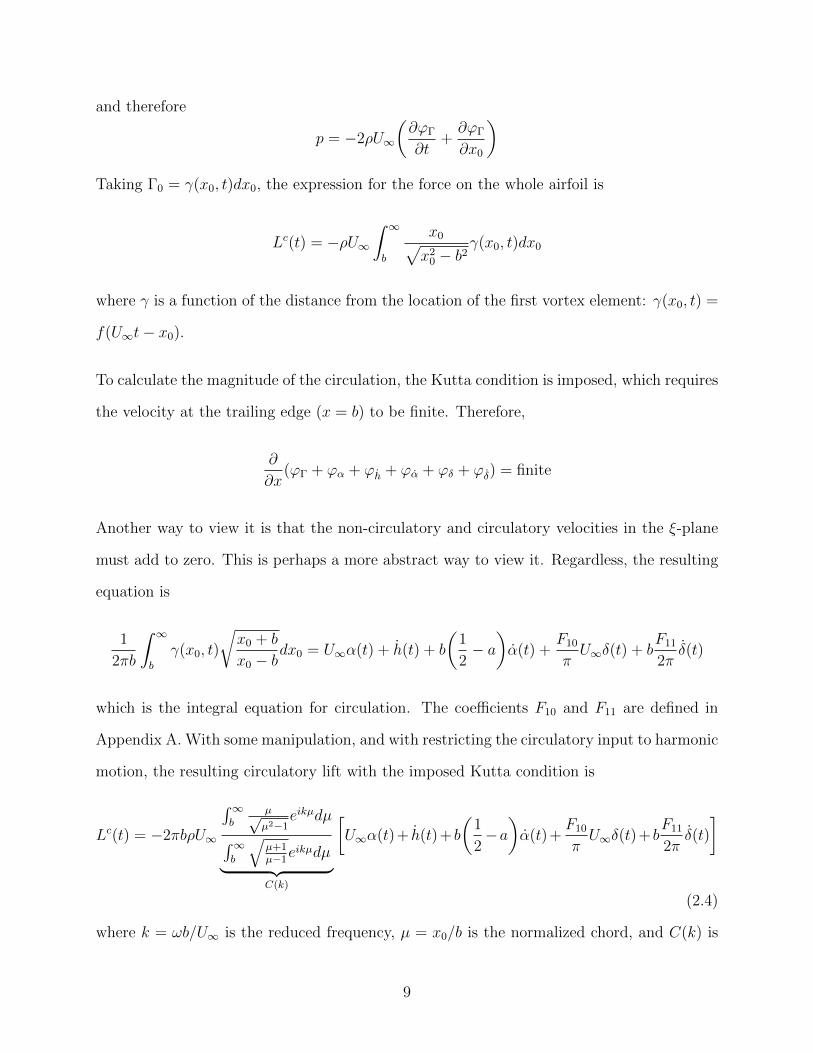
and therefore

p = −2ρU∞

(∂ϕΓ

∂t+∂ϕΓ

∂x0

)Taking Γ0 = γ(x0, t)dx0, the expression for the force on the whole airfoil is

Lc(t) = −ρU∞∫ ∞b

x0√x2

0 − b2γ(x0, t)dx0

where γ is a function of the distance from the location of the first vortex element: γ(x0, t) =

f(U∞t− x0).

To calculate the magnitude of the circulation, the Kutta condition is imposed, which requires

the velocity at the trailing edge (x = b) to be finite. Therefore,

∂

∂x(ϕΓ + ϕα + ϕh + ϕα + ϕδ + ϕδ) = finite

Another way to view it is that the non-circulatory and circulatory velocities in the ξ-plane

must add to zero. This is perhaps a more abstract way to view it. Regardless, the resulting

equation is

1

2πb

∫ ∞b

γ(x0, t)

√x0 + b

x0 − bdx0 = U∞α(t) + h(t) + b

(1

2− a)α(t) +

F10

πU∞δ(t) + b

F11

2πδ(t)

which is the integral equation for circulation. The coefficients F10 and F11 are defined in

Appendix A. With some manipulation, and with restricting the circulatory input to harmonic

motion, the resulting circulatory lift with the imposed Kutta condition is

Lc(t) = −2πbρU∞

∫∞b

µ√µ2−1

eikµdµ∫∞b

√µ+1µ−1

eikµdµ︸ ︷︷ ︸C(k)

[U∞α(t)+ h(t)+ b

(1

2−a)α(t)+

F10

πU∞δ(t)+ b

F11

2πδ(t)

]

(2.4)

where k = ωb/U∞ is the reduced frequency, µ = x0/b is the normalized chord, and C(k) is

9

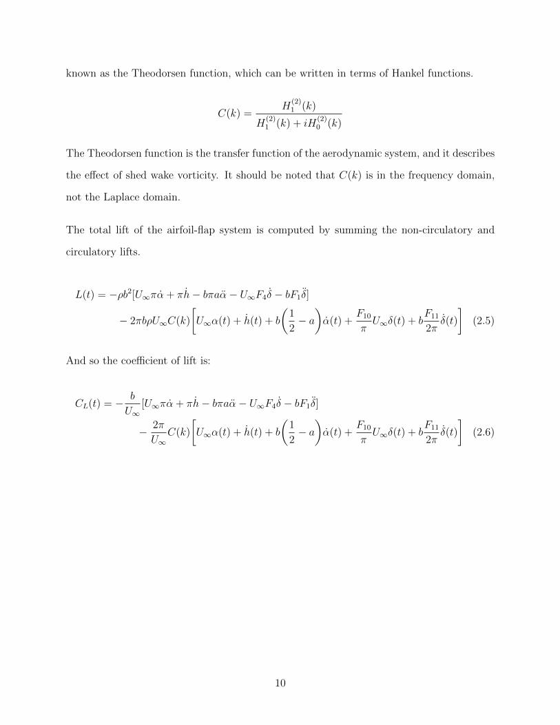
known as the Theodorsen function, which can be written in terms of Hankel functions.

C(k) =H

(2)1 (k)

H(2)1 (k) + iH

(2)0 (k)

The Theodorsen function is the transfer function of the aerodynamic system, and it describes

the effect of shed wake vorticity. It should be noted that C(k) is in the frequency domain,

not the Laplace domain.

The total lift of the airfoil-flap system is computed by summing the non-circulatory and

circulatory lifts.

L(t) = −ρb2[U∞πα + πh− bπaα− U∞F4δ − bF1δ]

− 2πbρU∞C(k)

[U∞α(t) + h(t) + b

(1

2− a)α(t) +

F10

πU∞δ(t) + b

F11

2πδ(t)

](2.5)

And so the coefficient of lift is:

CL(t) = − b

U∞[U∞πα + πh− bπaα− U∞F4δ − bF1δ]

− 2π

U∞C(k)

[U∞α(t) + h(t) + b

(1

2− a)α(t) +

F10

πU∞δ(t) + b

F11

2πδ(t)

](2.6)

10

Chapter 3

Leishman

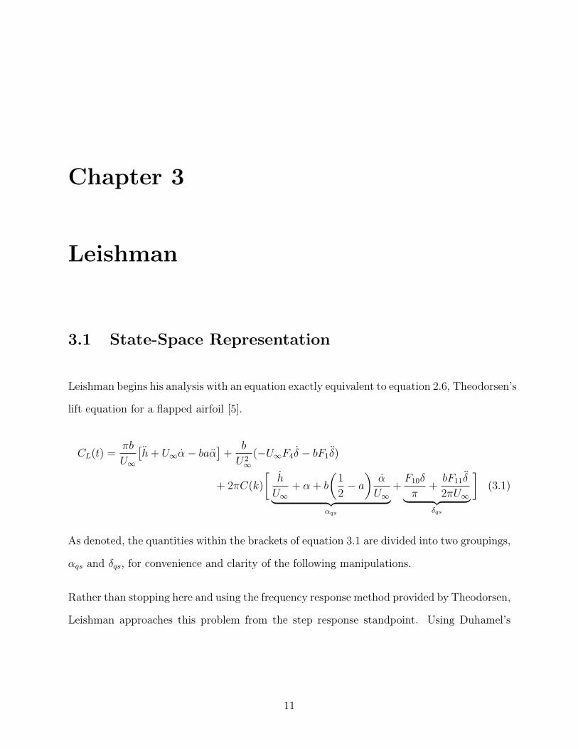
3.1 State-Space Representation

Leishman begins his analysis with an equation exactly equivalent to equation 2.6, Theodorsen’s

lift equation for a flapped airfoil [5].

CL(t) =πb

U∞

[h+ U∞α− baα

]+

b

U2∞

(−U∞F4δ − bF1δ)

+ 2πC(k)

[h

U∞+ α + b

(1

2− a)α

U∞︸ ︷︷ ︸αqs

+F10δ

π+bF11δ

2πU∞︸ ︷︷ ︸δqs

](3.1)

As denoted, the quantities within the brackets of equation 3.1 are divided into two groupings,

αqs and δqs, for convenience and clarity of the following manipulations.

Rather than stopping here and using the frequency response method provided by Theodorsen,

Leishman approaches this problem from the step response standpoint. Using Duhamel’s

11

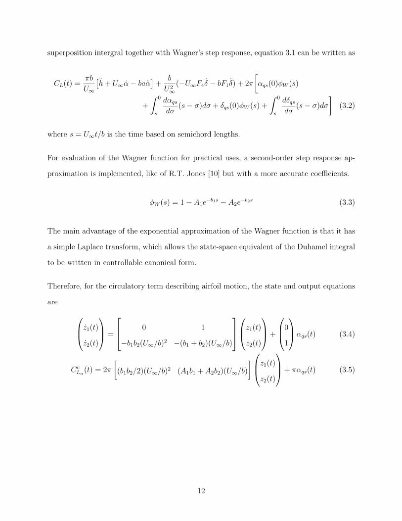
superposition intergral together with Wagner’s step response, equation 3.1 can be written as

CL(t) =πb

U∞

[h+ U∞α− baα

]+

b

U2∞

(−U∞F4δ − bF1δ) + 2π

[αqs(0)φW (s)

+

∫ 0

s

dαqsdσ

(s− σ)dσ + δqs(0)φW (s) +

∫ 0

s

dδqsdσ

(s− σ)dσ

](3.2)

where s = U∞t/b is the time based on semichord lengths.

For evaluation of the Wagner function for practical uses, a second-order step response ap-

proximation is implemented, like of R.T. Jones [10] but with a more accurate coefficients.

φW (s) = 1− A1e−b1s − A2e

−b2s (3.3)

The main advantage of the exponential approximation of the Wagner function is that it has

a simple Laplace transform, which allows the state-space equivalent of the Duhamel integral

to be written in controllable canonical form.

Therefore, for the circulatory term describing airfoil motion, the state and output equations

are z1(t)

z2(t)

=

0 1

−b1b2(U∞/b)2 −(b1 + b2)(U∞/b)

z1(t)

z2(t)

+

0

1

αqs(t) (3.4)

CcLα(t) = 2π

[(b1b2/2)(U∞/b)

2 (A1b1 + A2b2)(U∞/b)

]z1(t)

z2(t)

+ παqs(t) (3.5)

12

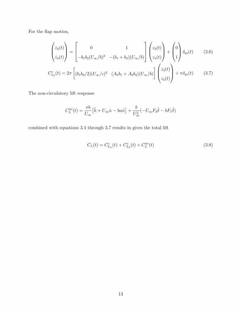
For the flap motion,

z3(t)

z4(t)

=

0 1

−b1b2(U∞/b)2 −(b1 + b2)(U∞/b)

z3(t)

z4(t)

+

0

1

δqs(t) (3.6)

CcLδ

(t) = 2π

[(b1b2/2)(U∞/c)

2 (A1b1 + A2b2)(U∞/b)

]z3(t)

z4(t)

+ πδqs(t) (3.7)

The non-circulatory lift response

CncL (t) =

πb

U∞

[h+ U∞α− baα

]+

b

U2∞

(−U∞F4δ − bF1δ)

combined with equations 3.4 through 3.7 results in gives the total lift

CL(t) = CcLα(t) + Cc

Lδ(t) + Cnc

L (t) (3.8)

13

Chapter 4

Garrick

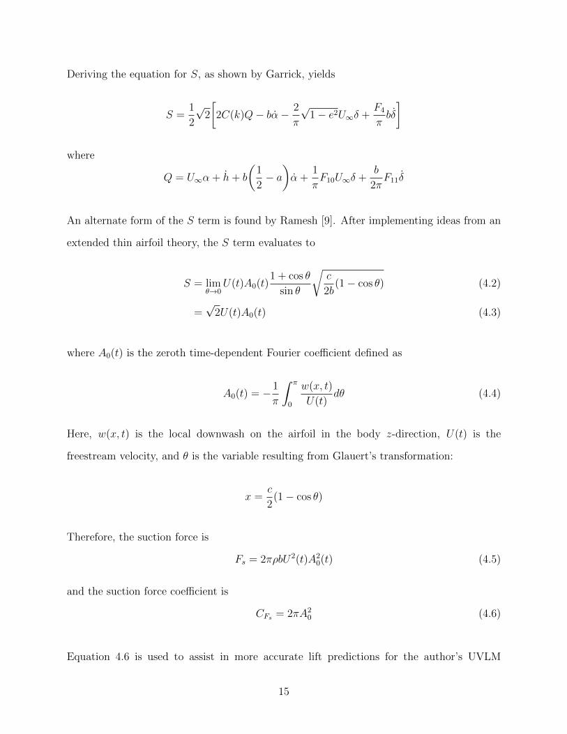
Garrick [2] uses Theodorsen’s analytical results and extends the derivation to include the

forces in the horizontal direction in order to calculation the thrust (or propulsive force). In

this paper, the drag forces are not the main focus, so the suction force is solely used to more

accurately predict the lift.

The suction force is defined as

FS = πρbS2 (4.1)

where S is obtained by the relation

S = limx→−1

γ(x)

√x+ 1

b

The value of S is finite since γ is infinite in the order of 1/√x+ 1 at the leading edge x = −1.

Due to this occurrence of infinity, it must be noted that ideal flow for an infinitely thin wing

is impossible, which is the reason Garrick views this case as a limiting one: the airfoil is

round and smooth at the leading edge but sharp at the trailing edge. Further explanation

can be found in reference [4] and [8].

14

Deriving the equation for S, as shown by Garrick, yields

S =1

2

√2

[2C(k)Q− bα− 2

π

√1− e2U∞δ +

F4

πbδ

]

where

Q = U∞α + h+ b

(1

2− a)α +

1

πF10U∞δ +

b

2πF11δ

An alternate form of the S term is found by Ramesh [9]. After implementing ideas from an

extended thin airfoil theory, the S term evaluates to

S = limθ→0

U(t)A0(t)1 + cos θ

sin θ

√c

2b(1− cos θ) (4.2)

=√

2U(t)A0(t) (4.3)

where A0(t) is the zeroth time-dependent Fourier coefficient defined as

A0(t) = − 1

π

∫ π

0

w(x, t)

U(t)dθ (4.4)

Here, w(x, t) is the local downwash on the airfoil in the body z-direction, U(t) is the

freestream velocity, and θ is the variable resulting from Glauert’s transformation:

x =c

2(1− cos θ)

Therefore, the suction force is

Fs = 2πρbU2(t)A20(t) (4.5)

and the suction force coefficient is

CFs = 2πA20 (4.6)

Equation 4.6 is used to assist in more accurate lift predictions for the author’s UVLM

15

calculations, as described in the following chapter.

16

Chapter 5

Unsteady Vortex Lattice Method

(UVLM)

The description presented here of the UVLM is much more extensive and detailed than that

of Theodorsen’s, Leishman’s, or Garrick’s work, since the numerical method is the author’s

work. The underlying methodology is more clearly outlined, beginning with a statement of

what is being addressed and followed with the fundamentals of the flow and specifics of the

UVLM. In general, this section of the article is a walkthrough of the code programmed using

the UVLM.

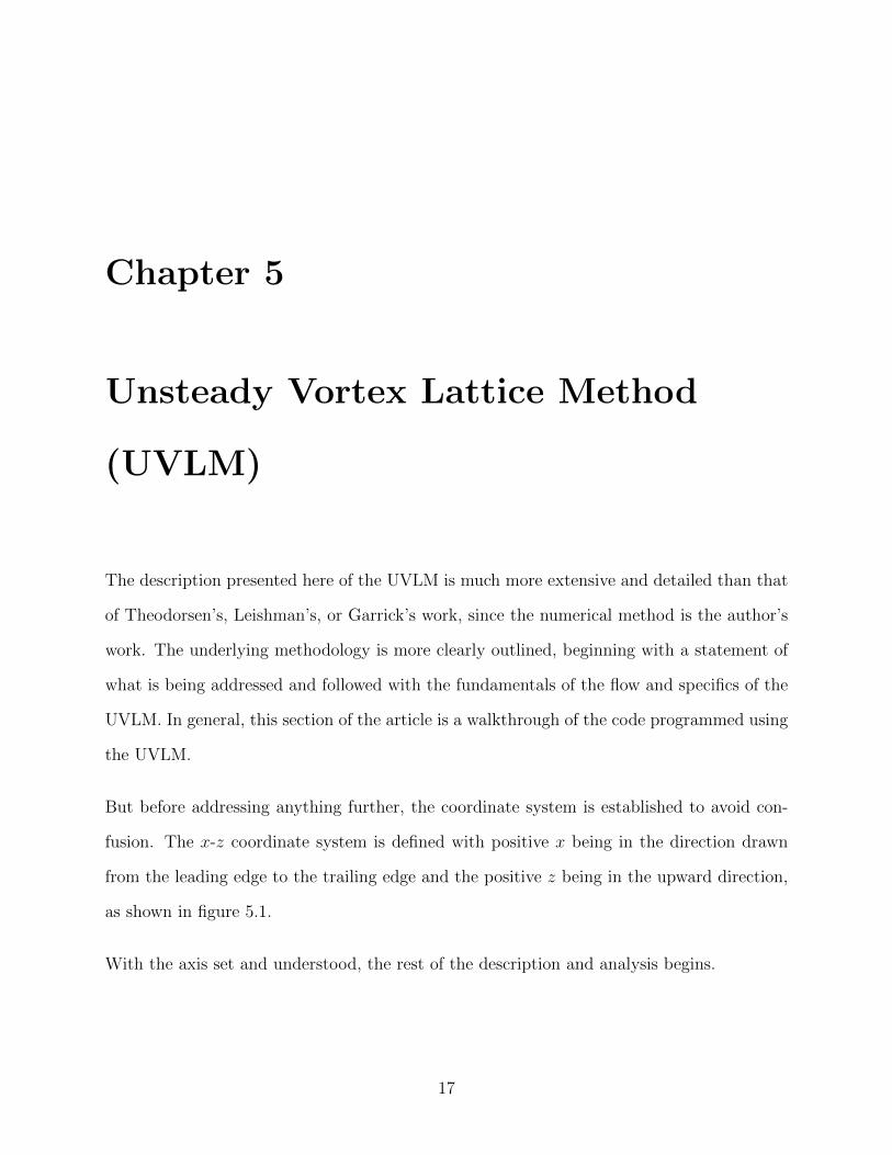
But before addressing anything further, the coordinate system is established to avoid con-

fusion. The x-z coordinate system is defined with positive x being in the direction drawn

from the leading edge to the trailing edge and the positive z being in the upward direction,

as shown in figure 5.1.

With the axis set and understood, the rest of the description and analysis begins.

17

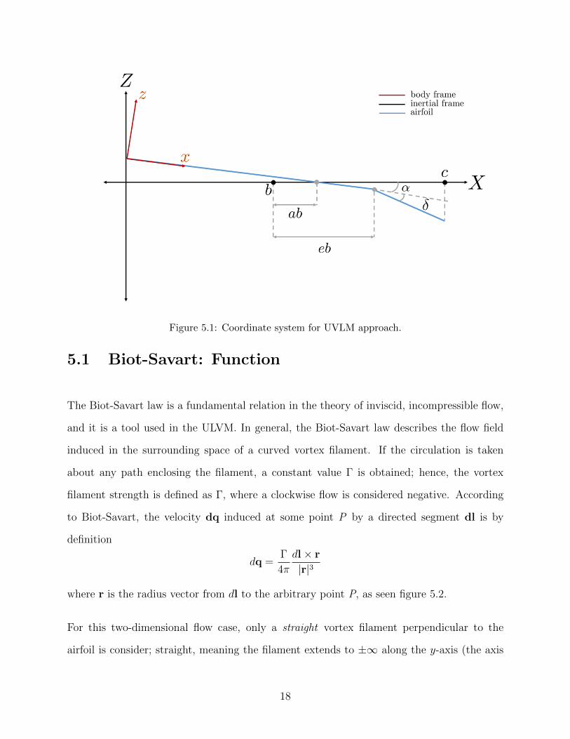
Figure 5.1: Coordinate system for UVLM approach.

5.1 Biot-Savart: Function

The Biot-Savart law is a fundamental relation in the theory of inviscid, incompressible flow,

and it is a tool used in the ULVM. In general, the Biot-Savart law describes the flow field

induced in the surrounding space of a curved vortex filament. If the circulation is taken

about any path enclosing the filament, a constant value Γ is obtained; hence, the vortex

filament strength is defined as Γ, where a clockwise flow is considered negative. According

to Biot-Savart, the velocity dq induced at some point P by a directed segment dl is by

definition

dq =Γ

4π

dl× r

|r|3

where r is the radius vector from dl to the arbitrary point P, as seen figure 5.2.

For this two-dimensional flow case, only a straight vortex filament perpendicular to the

airfoil is consider; straight, meaning the filament extends to ±∞ along the y-axis (the axis

18

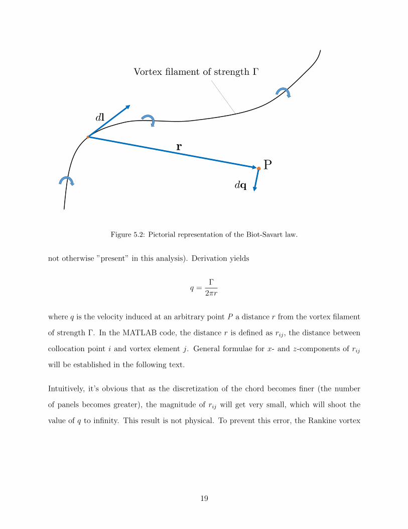
Figure 5.2: Pictorial representation of the Biot-Savart law.

not otherwise ”present” in this analysis). Derivation yields

q =Γ

2πr

where q is the velocity induced at an arbitrary point P a distance r from the vortex filament

of strength Γ. In the MATLAB code, the distance r is defined as rij, the distance between

collocation point i and vortex element j. General formulae for x- and z-components of rij

will be established in the following text.

Intuitively, it’s obvious that as the discretization of the chord becomes finer (the number

of panels becomes greater), the magnitude of rij will get very small, which will shoot the

value of q to infinity. This result is not physical. To prevent this error, the Rankine vortex

19

characterization of inviscid flow is implemented.

q(r) =

rΓ

2πR2 , if r ≤ R

Γ2πr, if r > R

Inside the core radius, as shown in figure 5.3, viscosity is modeled to exist; however, beyond

Figure 5.3: A look at the Rankine vortex model.

the core radius the flow is inviscid (i.e. potential flow exists). This combination of viscous

and inviscid flow allows for a more correct modeling of potential flow when using the Biot-

20

Savart law to describe vortex-point interactions.

5.2 Geometry

5.2.1 Time-Invariant Geometry: Lines 99-108

With a necessary tool understood, the geometry of the airfoil is defined. The full chord

length of the airfoil is denoted as c, and the flap portion of the chord is denoted as cf . The

ratio between cf and c is

λ =cfc

Therefore, the flat airfoil portion is defined as having a length of 1 − λ. Since the general

idea behind the UVLM is the discretization of otherwise continuous quantities in order to

numerically compute the output, the length of the airfoil (along with flap in the following

section) must be discretized.

The discretization and elements imposed cannot be arbitrary, however. Because the airfoil

of concern is thin, no sources are used, while the doublet distribution is approximated by n

doublet elements, which is equivalent to n concentrated vortices at the panel edges. With

prior knowledge of the geometry of the lumped vortex numerical method, it’s clear that

placing a vortex at the quarter chord (center of pressure) and a collocation point at the

three-quarter chord of the panel automatically satisfies the Kutta condition (γ(c, t) = 0).

Using this knowledge, the equivalent discretized model has the chord split into n panels, with

each segment having a vortex element and collocation point at its relative quarter chord and

three-quarter chord, respectively.

To find the number of panels found along the airfoil, the length of the airfoil is multiplied

21

with the total number of panels n along the entire chord.

K = (1− λ)n

The value of K must be an integer value. There can be no fractions of panels since there can

be no fractions of collocation points and vortex elements. (In this particular code, n must

be a multiple of four to run.)

With the foundation of the method set, two geometries are now considered: time-invariant

and time-varying. The location of the vortex elements xboundj and collocation points xcpi

are needed. The time-invariant geometry has the normal vector ni = constant with respect

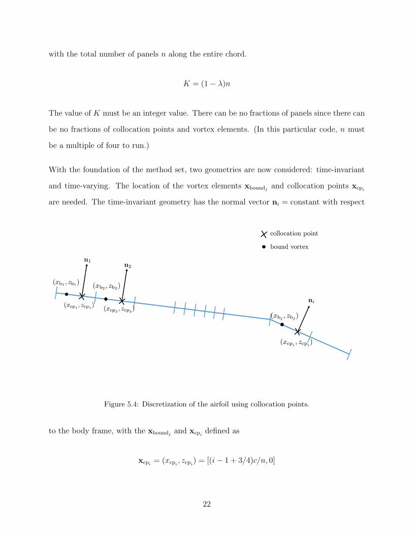
Figure 5.4: Discretization of the airfoil using collocation points.

to the body frame, with the xboundj and xcpi defined as

xcpi = (xcpi , zcpi) = [(i− 1 + 3/4)c/n, 0]

22

xboundj = (xbj , zbj) = [(j − 1 + 1/4)c/n, 0]

The z-value is zero here because there is no component of the plate in the z-direction of the

body frame for panels n = 1, 2, ..., K.

The distance between xcpi and xboundj is

rij = xcpi − xboundj = (xcpi , zcpi)− (xbj , zbj)

With this, the 2D numerical Biot-Savart equation is constructed.

qi =K∑j=1

Γj2πrij

(5.1)

This is physically the magnitude of the contribution of all the vortex elements at the collo-

cation point i. To find the contribution of all vortex elements on all the collocation points,

i is extended to run through the loop iterations of i = 1, 2, ..., K.

5.2.2 Time-Varying Geometry: Lines 134-148

The angle δ varies with time, so the geometry formulation is generalized to describe this.

The angle (with clockwise being negative) the flap creates with the airfoil is defined as

δ(t) = Aδ cosωδt

where ∆ is the amplitude, ωδ is the angular frequency of the flap motion, and t is the physical

time. The varying geometry due to flapping is characterized by

23

ni =

sin δ(t)

− cos δ(t)

xcpi =

c− cf0

+ (i−K − 1 + 3/4)cf

n−K

cos δ(t)

− sin δ(t)

xboundj =

c− cf0

+ (j −K − 1 + 1/4)cf

n−K

cos δ(t)

− sin δ(t)

with i = K + 1, K + 2, ..., n. This time-varying geometry formulation along with its time-

invariant analog gives the positions of all the collocation points and bound vortices, except

the starting vortex, which is exactly at the trailing edge of the flap:

xTE =

c− cf0

+ cf

cos δ(t)

− sin δ(t)

5.3 Kinematics: Lines 114-142

With the geometry known, the motion of the system is now addressed.

The vertical translational motion, known as plunging or heaving, is described by a sinusoidal

function

h(t) = H sin(ωht+ φh)

where H is the maximum heaving amplitude, ωh is the heaving angular frequency, φh is the

phase angle of the plunging motion, and t is the physical time; the former two are measured

relative to pivot point ab (described later).

24

Given an airfoil traveling with a velocity −U∞X, as defined in the inertial and negative

X-direction1, and taking into account the effects of plunging, the resultant velocity Qplunge,

as seen by the airfoil (body frame), is2

Qplunge =

−U∞ cosα− h sinα

−U∞ sinα + h cosα

where h is the time derivative of the vertical position due to plunging, and α is the angle of

attack.

The coupled airfoil pitching is defined as a rotation about a point on the chord c at a distance

ab from the midpoint of the chord, where a is the flip axis ratio; therefore, the instantaneous

angle of attack (as seen in the airfoil frame) measured counterclockwise from the mean chord

is

α(t) = αm + α0 sin(ωαt+ φα)

where αm is the mean pitch angle, φα is the phase angle of the pitching motion, α0 is the

maximum pitching amplitude, and ωα is the pitching angular frequency, the latter two of

which are taken about the pivot point a.

Taking both the plunging and pitching effects into account, the resultant velocity Qpp is

defined as

Qpp =

−U∞ cosα− h sinα

−U∞ sinα + h cosα− α(x− b(1 + a)

) (5.2)

where x is an arbitrary point along the body frame x-axis. In the code for the numerical

method, this ”arbitrary” point is a collocation point xcp on the camberline.

1Notice that the inertial coordinate frame is denoted by capital letters, whereas as the body frame isdenoted with lower-case letters.

2Note that all vectors in this paper are written in the conventional column vector format, whereas thevectors in the MATLAB code are typed in the row vector format. Be sure to remember this distinction whencomparing the theory found in this paper to the code.

25

Note that when comparing this analytical result to the code, it is obvious that the pitching

effect is not present initially; the code implements the pitching effect at a later section. This

is due only to convenience, not necessity. It’s easier to insert the pitching effect after the

influence coefficient matrix aij has been created.

5.4 Influence Coefficient Matrix (ICM): Lines 150-160

To begin the derivation of the influence coefficient matrix3 [11], the no-penetration boundary

condition is imposed.

(∇ΦB +∇ΦW −V0 − vrel −Ω× r) · n = 0

Here, the perturbation potential Φ is divided into the airfoil potential ΦB and the wake

potential ΦW . Defining the other terms: V0 is the velocity of the body (airfoil) system’s

origin relative to the inertial frame, vrel is the velocity relative to the body frame, r is the

position vector, Ω is the rate of rotation of the body’s frame of reference, and n is the vector

normal to the airfoil’s surface.

The above equation is made into the left-hand side (LHS), which includes the potentials,

and the right-hand side (RHS), which includes the kinematic velocity due to the motion of

the airfoil and the velocity components induced by the wake.

LHS ≡ (∇ΦB +∇ΦW ) · n = −(−V0 − vrel −Ω× r) · n ≡ RHS (5.3)

The self-induced portion (∇ΦB · n) is established by first considering the influence due to

a unit strength circulation Γj, which yields the influence coefficient aij in this numerical

3The following derivation is taken almost completely from Chapter 9 and 13 of Low Speed Aerodynamics,by Katz and Plotkin.

26

method.

aij = ∇ΦBij |(Γ=1) · ni

This shows ∇ΦBij = qij = (u,w)ij, which is the velocity component at collocation point i

induced by the unit strength singularity element j.

The x- and z-components are determined by the Biot-Savart law as follows:

uij =Γj2π

zcpi − zbj

r2ij

=Γj2π

zcpi − zbj

(xcpi − xbj)2 + (zcpi − zbj)

2

wij =Γj2π

xcpi − xbj

r2ij

=Γj2π

xcpi − xbj

(xcpi − xbj)2 + (zcpi − zbj)

2

Notice that there is not a negative sign on the wi value. That’s because, as stated before,

the positive z-direction points downwards.

As a reminder, since the vortex strengths Γ are unknown (and will be calculated for), Γ = 1

is taken to determine the induced velocity used in the evaluation of the influence coefficients.

uij =1

2π

zcpi − zbj

(xcpi − xbj)2 + (zcpi − zbj)

2

wij =1

2π

xcpi − xbj

(xcpi − xbj)2 + (zcpi − zbj)

2

Therefore, the induced velocity created by vortex j on collocation point i by a unit strength

Γ is4

qij =1

2π[(xcpi − xbj)2 + (zcpi − zbj)

2]

zcpi − zbj

xcpi − xbj

(5.4)

Using this equation, the aij’s are found.

aij = qij · ni = qTijni (5.5)

4The following equation is the equation used in the Biot-Savart function of the MATLAB code.

27

Equation 5.5 is the general equation for finding the influence coefficients. Variations in

geometry must be accounted for.

Next, the wake-induced portion of equation 5.3 is established by taking into account the

influence due to a unit strength wake circulation ΓWt , yielding

aiwt = ∇ΦWi· ni = qiwt|(Γ=1) · ni

Considering both the self-induced and wake-induced portions results in the equation for the

LHS.

LHS ≡ (∇ΦB +∇ΦW ) · n =n∑j=1

aijΓj + aiWtΓWt (5.6)

with i = 1, 2, 3..., n, and ΓWt being the strength of the latest vortex. Note that this entire

calculation is carried out at a single time t. (In the code, time steps are denoted by the

letter k.) In matrix form, the LHS is written as

LHS ≡

a11 a12 a13 . . . a1n a1w

a21 a22 a23 . . . a2n a2w

......

.... . .

......

an1 an2 an3 . . . ann anW

1 1 1 . . . 1 1

Γ1

Γ2

...

Γn

ΓWt

(5.7)

The LHS is complete, so the RHS is addressed next. The terms (−V0 − vrel − Ω × r)

are replaced with with two groupings of terms: 1) an equivalent tangential and normal

velocity [U(t),W (t)]i, representing the kinematic motion of the airfoil; and 2) the velocity

components induced by the wake vortices (uW , wW )i, not including the velocity induced by

the latest vortex.

To complete the RHS, the law of zero total circulation (Kelvin’s Circulation Theorem) is

28

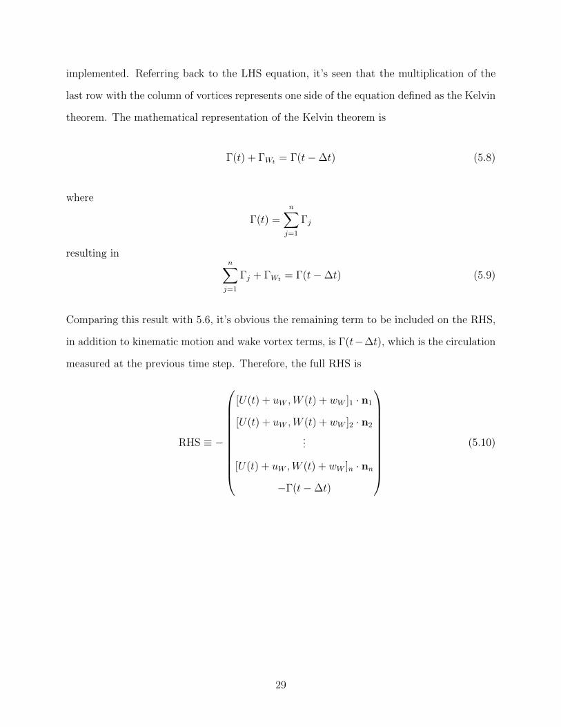
implemented. Referring back to the LHS equation, it’s seen that the multiplication of the

last row with the column of vortices represents one side of the equation defined as the Kelvin

theorem. The mathematical representation of the Kelvin theorem is

Γ(t) + ΓWt = Γ(t−∆t) (5.8)

where

Γ(t) =n∑j=1

Γj

resulting inn∑j=1

Γj + ΓWt = Γ(t−∆t) (5.9)

Comparing this result with 5.6, it’s obvious the remaining term to be included on the RHS,

in addition to kinematic motion and wake vortex terms, is Γ(t−∆t), which is the circulation

measured at the previous time step. Therefore, the full RHS is

RHS ≡ −

[U(t) + uW ,W (t) + wW ]1 · n1

[U(t) + uW ,W (t) + wW ]2 · n2

...

[U(t) + uW ,W (t) + wW ]n · nn

−Γ(t−∆t)

(5.10)

29

Equating the 5.7 and 5.10 gives

a11 a12 a13 . . . a1n a1W

a21 a22 a23 . . . a2n a2W

......

.... . .

......

an1 an2 an3 . . . ann anW

1 1 1 . . . 1 1

Γ1

Γ2

...

Γj

ΓWt

= −

[U(t) + uW ,W (t) + wW ]1 · n1

[U(t) + uW ,W (t) + wW ]2 · n2

...

[U(t) + uW ,W (t) + wW ]n · nn

−Γ(t−∆t)

(5.11)

5.5 Right Hand Side: Lines 163-179

Though equation 5.11 is established, the entries of the RHS are yet unknown. To determine

the values of the entries, the airfoil is viewed as a whole. First, the plunging motion of the

airfoil is considered, taking the form

Qplunge =

−U∞ cosα− h sinα

−U∞ sinα + h cosα

(5.12)

Pitching is then added, yielding

Qpp =

−U∞ cosα− h sinα

−U∞ sinα + h cosα− α(x− b(1 + a)

)

where the pp subscript denotes pitch-plunge.

By way of reminder, the terms on the RHS are (−V0 − vrel − Ω × r). These are replaced

with the equivalent [U(t) + uW ,W (t) + wW ] terms, which include the kinematic velocities

and the wake-induced velocities. The equation for Qpp takes into account only the kinematic

velocity; wake-induced velocities are added. These two portions of the RHS are denoted as

30

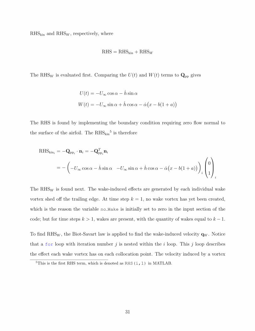
RHSkin and RHSW , respectively, where

RHS = RHSkin + RHSW

The RHSW is evaluated first. Comparing the U(t) and W (t) terms to Qpp gives

U(t) = −U∞ cosα− h sinα

W (t) = −U∞ sinα + h cosα− α(x− b(1 + a)

)The RHS is found by implementing the boundary condition requiring zero flow normal to

the surface of the airfoil. The RHSkin5 is therefore

RHSkini = −Qppi · ni = −QTppi

ni

= −(−U∞ cosα− h sinα −U∞ sinα + h cosα− α

(x− b(1 + a)

))i

0

1

i

The RHSW is found next. The wake-induced effects are generated by each individual wake

vortex shed off the trailing edge. At time step k = 1, no wake vortex has yet been created,

which is the reason the variable no Wake is initially set to zero in the input section of the

code; but for time steps k > 1, wakes are present, with the quantity of wakes equal to k− 1.

To find RHSW , the Biot-Savart law is applied to find the wake-induced velocity qW . Notice

that a for loop with iteration number j is nested within the i loop. This j loop describes

the effect each wake vortex has on each collocation point. The velocity induced by a vortex

5This is the first RHS term, which is denoted as RHS(i,1) in MATLAB.

31

of strength ΓW is

qW =ΓW2π

1

[(xcpi − xWj)2 + (zcpi − zWj

)2]

zcpi − zWj

xcpi − xWj

(5.13)

where j = 1, 2, ..., k, with j denoting the wake vortex number in this instance.

RHSWiis found by using the familiar relationship

RHSWi= −qWi

· ni = −qTWini

= −ΓW2π

1

[(xcpi − xWj)2 + (zcpi − zWj

)2]

(zcpi − zWj

xcpi − xWj

)0

1

i

The RHS is computed by summing the kinematic RHS with the wake-induced RHS:

RHSi = RHSkini + RHSWi(5.14)

This is done on the final line of the nested j loop. The j loop is then exited, followed by the

exiting of the i loop.

5.6 Solving the System: Lines 182-234

The main point of this section is to solve for the previously unknown Γ’s and to find the CL

and CT generated. That requires the pressure coefficient to first be found.

32

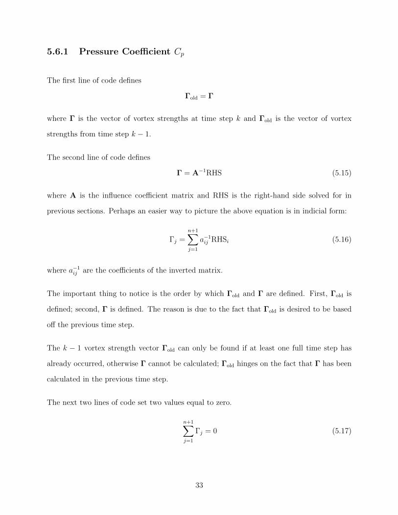
5.6.1 Pressure Coefficient Cp

The first line of code defines

Γold = Γ

where Γ is the vector of vortex strengths at time step k and Γold is the vector of vortex

strengths from time step k − 1.

The second line of code defines

Γ = A−1RHS (5.15)

where A is the influence coefficient matrix and RHS is the right-hand side solved for in

previous sections. Perhaps an easier way to picture the above equation is in indicial form:

Γj =n+1∑j=1

a−1ij RHSi (5.16)

where a−1ij are the coefficients of the inverted matrix.

The important thing to notice is the order by which Γold and Γ are defined. First, Γold is

defined; second, Γ is defined. The reason is due to the fact that Γold is desired to be based

off the previous time step.

The k − 1 vortex strength vector Γold can only be found if at least one full time step has

already occurred, otherwise Γ cannot be calculated; Γold hinges on the fact that Γ has been

calculated in the previous time step.

The next two lines of code set two values equal to zero.

n+1∑j=1

Γj = 0 (5.17)

33

n+1∑j=1

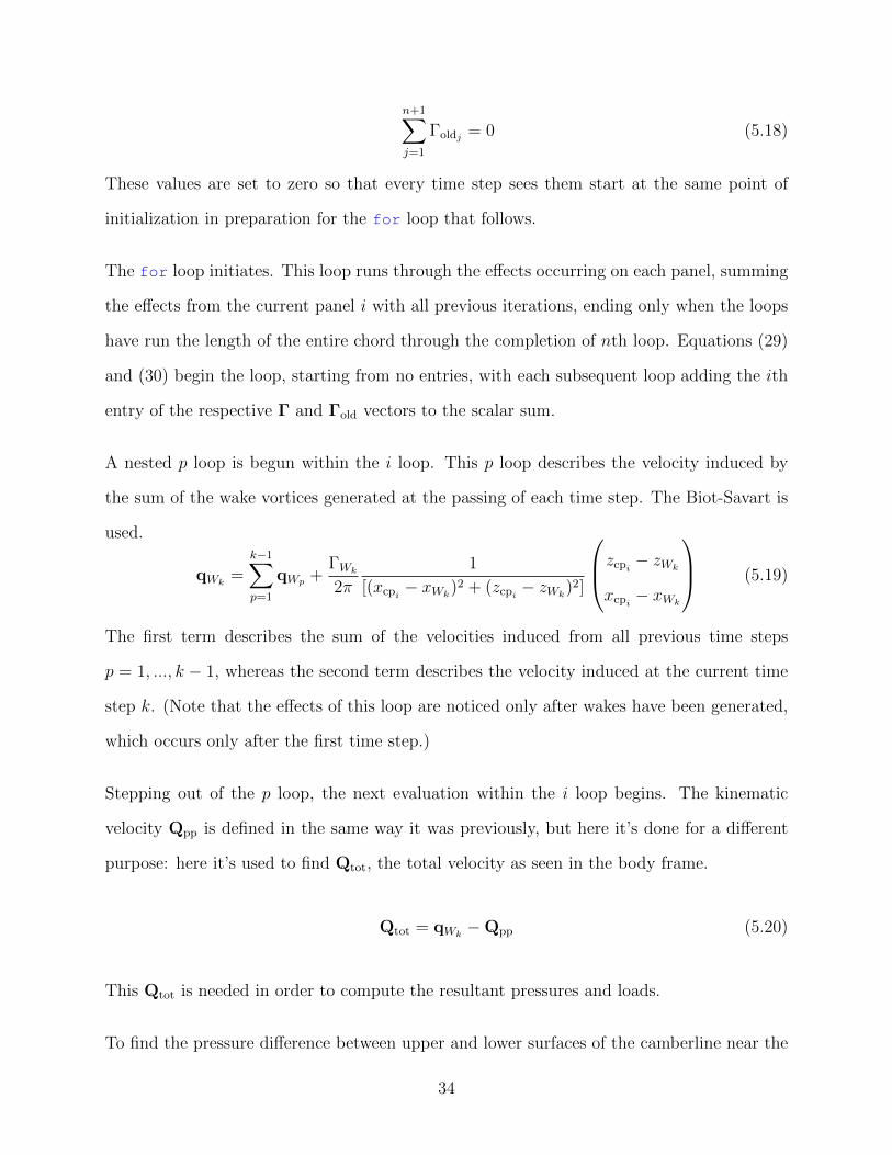
Γoldj = 0 (5.18)

These values are set to zero so that every time step sees them start at the same point of

initialization in preparation for the for loop that follows.

The for loop initiates. This loop runs through the effects occurring on each panel, summing

the effects from the current panel i with all previous iterations, ending only when the loops

have run the length of the entire chord through the completion of nth loop. Equations (29)

and (30) begin the loop, starting from no entries, with each subsequent loop adding the ith

entry of the respective Γ and Γold vectors to the scalar sum.

A nested p loop is begun within the i loop. This p loop describes the velocity induced by

the sum of the wake vortices generated at the passing of each time step. The Biot-Savart is

used.

qWk=

k−1∑p=1

qWp +ΓWk

2π

1

[(xcpi − xWk)2 + (zcpi − zWk

)2]

zcpi − zWk

xcpi − xWk

(5.19)

The first term describes the sum of the velocities induced from all previous time steps

p = 1, ..., k − 1, whereas the second term describes the velocity induced at the current time

step k. (Note that the effects of this loop are noticed only after wakes have been generated,

which occurs only after the first time step.)

Stepping out of the p loop, the next evaluation within the i loop begins. The kinematic

velocity Qpp is defined in the same way it was previously, but here it’s done for a different

purpose: here it’s used to find Qtot, the total velocity as seen in the body frame.

Qtot = qWk−Qpp (5.20)

This Qtot is needed in order to compute the resultant pressures and loads.

To find the pressure difference between upper and lower surfaces of the camberline near the

34

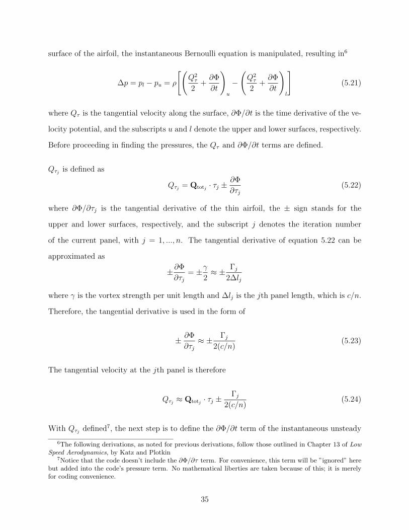
surface of the airfoil, the instantaneous Bernoulli equation is manipulated, resulting in6

∆p = pl − pu = ρ

[(Q2τ

2+∂Φ

∂t

)u

−

(Q2τ

2+∂Φ

∂t

)l

](5.21)

where Qτ is the tangential velocity along the surface, ∂Φ/∂t is the time derivative of the ve-

locity potential, and the subscripts u and l denote the upper and lower surfaces, respectively.

Before proceeding in finding the pressures, the Qτ and ∂Φ/∂t terms are defined.

Qτj is defined as

Qτj = Qtotj · τj ±∂Φ

∂τj(5.22)

where ∂Φ/∂τj is the tangential derivative of the thin airfoil, the ± sign stands for the

upper and lower surfaces, respectively, and the subscript j denotes the iteration number

of the current panel, with j = 1, ..., n. The tangential derivative of equation 5.22 can be

approximated as

±∂Φ

∂τj= ±γ

2≈ ± Γj

2∆lj

where γ is the vortex strength per unit length and ∆lj is the jth panel length, which is c/n.

Therefore, the tangential derivative is used in the form of

± ∂Φ

∂τj≈ ± Γj

2(c/n)(5.23)

The tangential velocity at the jth panel is therefore

Qτj ≈ Qtotj · τj ±Γj

2(c/n)(5.24)

With Qτj defined7, the next step is to define the ∂Φ/∂t term of the instantaneous unsteady

6The following derivations, as noted for previous derivations, follow those outlined in Chapter 13 of LowSpeed Aerodynamics, by Katz and Plotkin

7Notice that the code doesn’t include the ∂Φ/∂τ term. For convenience, this term will be ”ignored” herebut added into the code’s pressure term. No mathematical liberties are taken because of this; it is merelyfor coding convenience.

35

Bernoulli equation.

To find this velocity potential time derivative, a more fundamental definition is referenced

first: the velocity potential.

Φ± = ±∫∂Φ

∂τdτ

Applying the same approximation for the tangential derivative as used previously results in

Φ± = ±∫γ

2dτ = ±1

2

∫Γ

dτdτ

Therefore, the velocity potential time derivative is

±∂Φ

∂t= ± ∂

∂t

(1

2

∫Γ

dτdτ)

which, for a numerical method, takes the form

± ∂Φ

∂t= ±1

2

∂

∂t

j∑h=1

Γh (5.25)

This equation defines the local potential as the vortices are summed from the leading edge

to the jth vortex element along the camberline.

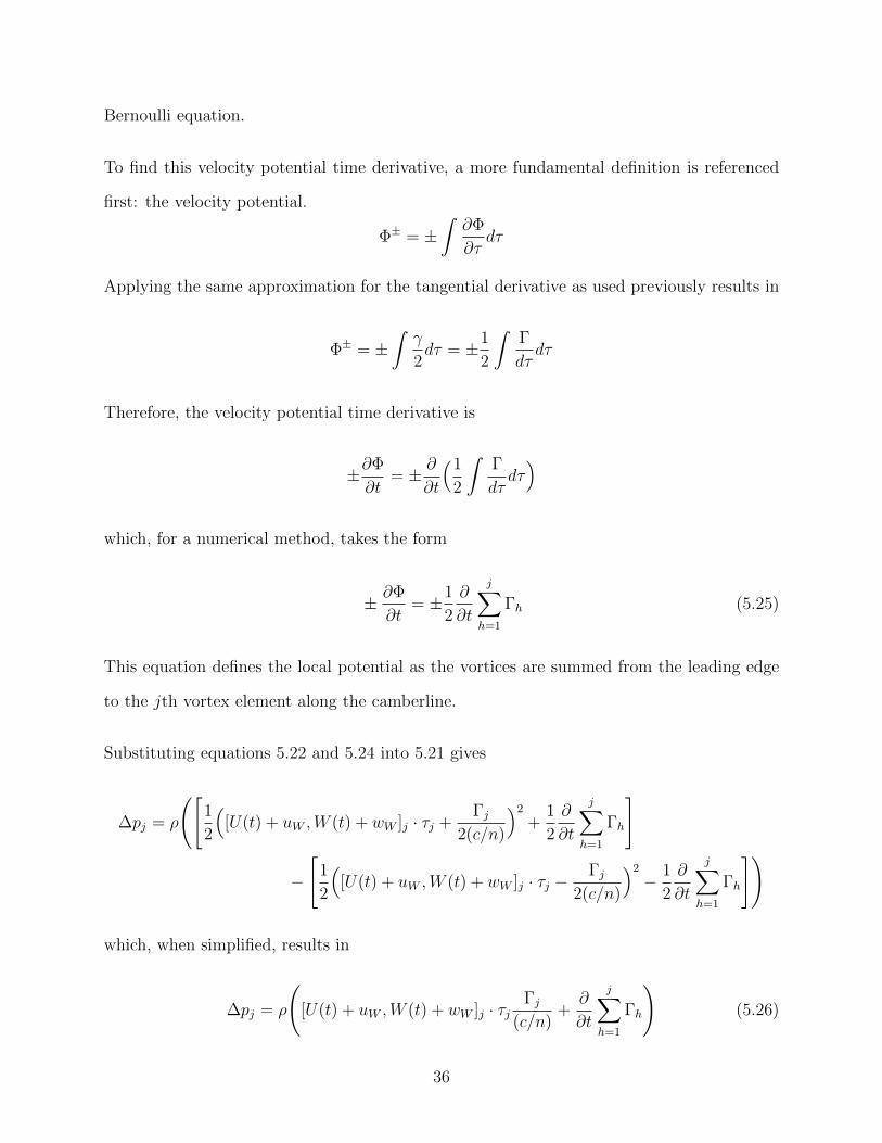
Substituting equations 5.22 and 5.24 into 5.21 gives

∆pj = ρ

([1

2

([U(t) + uW ,W (t) + wW ]j · τj +

Γj2(c/n)

)2

+1

2

∂

∂t

j∑h=1

Γh

]

−

[1

2

([U(t) + uW ,W (t) + wW ]j · τj −

Γj2(c/n)

)2

− 1

2

∂

∂t

j∑h=1

Γh

])

which, when simplified, results in

∆pj = ρ

([U(t) + uW ,W (t) + wW ]j · τj

Γj(c/n)

+∂

∂t

j∑h=1

Γh

)(5.26)

36

To determine the numerical form of the partial derivative, consider the definition of the

standard derivative.

dΓ(t)

dt= lim

∆t→0

Γ(t)− Γ(t−∆t)

∆t

In a numerical method, the ∆t doesn’t tend to zero but is rather a discrete finite number,

which will be kept in its denoted form of ∆t; and, since Γ is a function of time, the partial

derivative is the same as the standard derivative. The resultant numerical approximation is

therefore

∂

∂t

j∑h=1

Γh =1

∆t

j∑h=1

[Γh,k − Γh,k−1

](5.27)

where k denotes the current time step of evaluation. Plugging the above equation into the

pressure equation yields the following pressure coefficient:

∆Cpj =2

U2∞

([U(t) + uW ,W (t) + wW ]j · τj

Γj(c/n)

+1

∆t

j∑h=1

[Γh,k − Γh,k−1

])(5.28)

This is the equation used in the code to find the pressure difference between the upper and

lower surfaces.

5.6.2 Lift Coefficient CL

The lift is determined using the pressure equation, since lift is simply the force in the upward

direction generated by the pressure difference. For added accuracy in the lift prediction, the

suction force calculated by Garrick and reformulated by Ramesh is added onto the lift value

obtained by the pressure difference using equation (4.6). Calculation is split into two portions

due to there being two sections of the airfoil-flap system: 1) the airfoil; 2) the flap.

1. For the airfoil section (j ≤ K), only the pitch angle must be taken into account in

37

order to rectify the force into the inertial frame.

CL =K∑j=1

∆Cpjc

ncosαk + CFs sinαk (5.29)

2. The second section consists of the flap (j > K), which means both the pitch angle α(t)

and the flap angle δ(t) are considered in order to accurately describe the lift.

CL =n∑

j=K

∆Cpjc

ncos(αk + δk) + CFs sinαk (5.30)

These two portions of lift are handled by an if loop based on the iteration j.

5.7 Convection: Lines 237-270

The first for loop of this section generates the wake vector ΓW , with the number of entries

equal to the number of wake vortices from all previous time steps k − 1.

The number of wake vortices is equal to the number of time steps minus one.

nW = k − 1 (5.31)

The reason the number of vortices is not equal to the number of times steps is because

unsteady flow doesn’t elicit an instantaneous response. In other words, at k = 1, when the

airfoil motion initiates, the starting vortex is not instantly developed in its entirety. Only

after the first increment of time has passed is a starting vortex fully generated, and only

then are its effects accounted for. The MATLAB code is written to take into account this

lag.

38

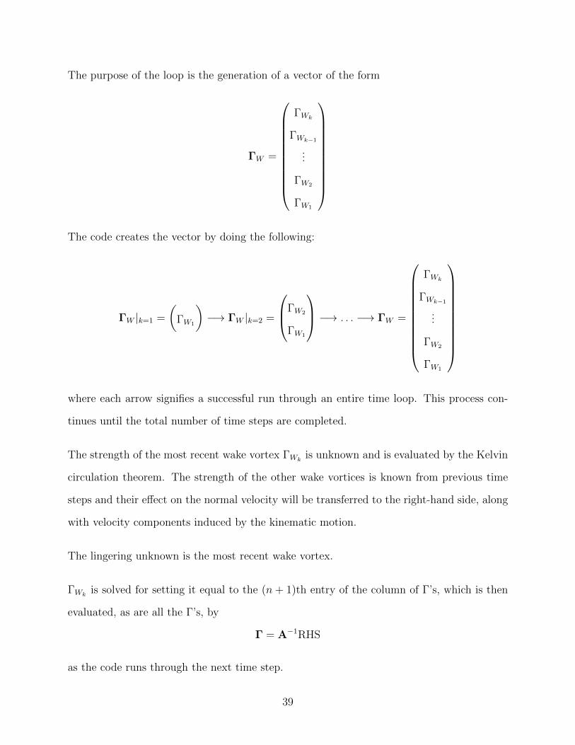
The purpose of the loop is the generation of a vector of the form

ΓW =

ΓWk

ΓWk−1

...

ΓW2

ΓW1

The code creates the vector by doing the following:

ΓW |k=1 =

(ΓW1

)−→ ΓW |k=2 =

ΓW2

ΓW1

−→ . . . −→ ΓW =

ΓWk

ΓWk−1

...

ΓW2

ΓW1

where each arrow signifies a successful run through an entire time loop. This process con-

tinues until the total number of time steps are completed.

The strength of the most recent wake vortex ΓWkis unknown and is evaluated by the Kelvin

circulation theorem. The strength of the other wake vortices is known from previous time

steps and their effect on the normal velocity will be transferred to the right-hand side, along

with velocity components induced by the kinematic motion.

The lingering unknown is the most recent wake vortex.

ΓWkis solved for setting it equal to the (n + 1)th entry of the column of Γ’s, which is then

evaluated, as are all the Γ’s, by

Γ = A−1RHS

as the code runs through the next time step.

39

For emphasis, it’s best to state again that the most recent vortex cannot be known at the

current time step. For example, ΓWkcannot be known at time step k, but it can be known

at time step k + 1. Another way to say it is: at time step k, only wake vortices up to ΓWk−1

can be known.

The next line of code: a summation of the entries of the wake vortex ΓW . Notice the

placement of this line. It comes near the end of the time loop, at a point after influence

coefficient matrix, after the right-hand side, and the lift have been calculated. It comes after

the prominent calculations have been completed. Therefore, in essence, this sum collects all

the wake vortices from the previous times steps.

For this concept to avoid confusion, actual placement of this line of code within the MATLAB

file should be ignored. Even though its appearance and evaluation is in the current time

step k, its purpose is not implemented until the following time step k + 1; so, in effect, it is

the sum of the wake circulation from previous time steps, which is the following:

k−1∑h=1

ΓWh= Γ(t−∆t)

When placed into what has already been written as the Kelvin theorem, the result is

n∑j=1

Γj + ΓWk=

k−1∑h=1

ΓWh(5.32)

with the only unknown being ΓWk(which, again, will be solved for at k + 1).

The method for finding the strengths of the vortices is now defined, but that’s useless until

the positions of those vortices are known. Remember, the velocity induced on the airfoil by

the vortices obeys the Biot-Savart law, a law that depends on the distance between a vortex

and a point.

The next line of code (skipping over the already-defined nW ) gives an array filled with the

40

positions of the wakes vortices.

xW =

xWkxWk−1

. . . xW2 xW1

zWkzWk−1

. . . zW2 zW1

(5.33)

where xWk= xbn+1 . This line takes all the wakes vortices from the previous time steps and

adds another entry corresponding to the wake vortex generated at the current time step.

Note that although the strength of the most recent vortex is not known, the position is

known; it always originates at the trailing edge of the airfoil.

Next, another for loop is created, which accounts for two things: 1) the translational velocity

of the wake vortices relative to the body frame; 2) the distance between the airfoil and the

wake vortices.

1. The first line in this loop re-equates the overall airfoil velocity with the velocity of pure

plunging motion, effectively removing the pitching term. The second line adds in a

new pitching term

−α(xW − b(1 + a)

)which is with respect to the positions of the wake vortices. Together, these two lines

give the velocity of the wake vortices relative to the body frame.

2. The final line of code in this loop defines the resultant positions of all the wake vortices

relative to the body frame after the cycle of the current time step k. The equation is

xWnew = xW −Qpp∆t (5.34)

where ∆t is the change in time from the previous time step k − 1 to the current step

k.

There are two loops left in the code, both of which use the Biot-Savart law.

41

The first loop describes the contribution of the velocity induced by the bound vortices on

the wake vortices. The equation takes the following form:

qWi,bj =Γj2π

1

[(xWi− xbj)

2 + (zWi− zbj)

2]

zWi− zbj

xWi− xbj

(5.35)

where the subscript attached the to the q term denoting the bound-on-wake vortex effect.

To get the new position of the wake vortices, the following is implemented:

xWnew = xWnew + qWi,bj∆t

which yields a wake vortex position that takes into account the induced velocity effects of

the bound vortices on the wake vortices.

The second loop describes the contribution of the velocity induced by the wake vortices on

the wake vortices.

qWi,Wj=

Γj2π

1

[(xWi− xWj

)2 + (zWi− zWj

)2]

zWi− zWj

xWi− xWj

(5.36)

where the subscript attached to the q term denotes the wake-on-wake vortex effect. To get

the new ”final” position of the wake vortices within the current time loop, the same method

is implemented.

xWnew = xWnew + qWi,Wj∆t

With both bound-on-wake and wake-on-wake effects taken into account, the final wake vortex

vector xWnew is known, which describes the position of every wake vortex relative to the body

frame at the completion of the current time step.

One more thing remains. In order to properly take advantage of MATLAB’s iterative abil-

ities, the final wake vortex vector xWnew is redefined as the initial wake vortex vector xW

42

before sending it into the (k + 1)th time step.

xWnew = xW

The code is now complete, and the theory behind it should be clear.

43

Chapter 6

Results

As a brief introduction to this chapter, let it be noted that the results obtained are for three

strict cases: 1) plunging with amplitude H = 0.02b1; 2) pitching with amplitude |α| = 3

and pitch axis location at the quarter chord (a = −0.25); and 3) flapping with amplitude

|δ| = 5 and with hinge axis at the three-quarter chord (e = 0.5).

6.1 Verification

In order to validate a numerical method, it is compared to analytical or experimental data.

Since only analytical data is addressed here, the UVLM is contrained to be checked against

mathematics.

However, before anything is validated, the analytical method is first verified to have been

coded properly by the author. Theodorsen’s paper does not contain a plot illustrating lift

1For the plunging case constrained by the parameter H = 0.02b, the effective angle of attack becomesgreater than 5 at k > 4.3, which is the healthy angle limit of the methods based on thin airfoil theory.However, for the sake of equal comparison, the plunging case was tested all the way through k = 10, as werepitching and flapping.

44

versus, while Leishman’s does. That said, how are both methods to be verified if only one

is represented graphically?

It is good to remember that the difference between Theordorsen’s and Leishman’s formu-

lations of lift is that the former is based on frequency response and the latter is based on

indicial (step) response. Since Theordorsen’s function and Wagner’s function (used in Leish-

man’s derivation) are related by means of a Fourier transform pair, the resulting lift from

both methods will be almost exactly the same. Therefore, for the accuracy required in this

paper, verification of Leishman’s data is, by extension, verification of Theodorsen’s.

The below figure shows the data digitized directly from Leishman’s paper. On top of the

digitized data are the plots generated in MATLAB. Since Leishman’s method requires direct

integration, the author makes use of MATLAB’s built-in ordinary differential equation solver

ode45, which implements the fourth/fifth-order Runge-Kutta method and therefore has

variable step size. (Note that the state equations are integrated with respect to time.)

In figure 6.12, the dotted lines denote the digitized data and the solid lines denote the

results outputted from the author’s code. As can be seen, both align nearly on top of

each other3. Though there are slight differences in phase, the discrepancies are due to

the inaccuracies inherent to the digitization process when using the GRABIT downloadable

MATLAB function. Such errors are well within the tolerable range; therefore, the code of

the analytical formulation is verified to accurately represent Theodorsen’s and Leishman’s

expressions.

2A nonlinear fit function nlinfit is used in MATLAB to produce the smooth plots seen here. Withoutthe fit, the ode45 function results in a jagged shape, likely due to its built-in time interval scheme.

3The code based on Theodorsen’s formulation s used for k = 0.01. The reason is that Leishman’sformulation does not give an accurate result. More on this is presented in the next section.

45

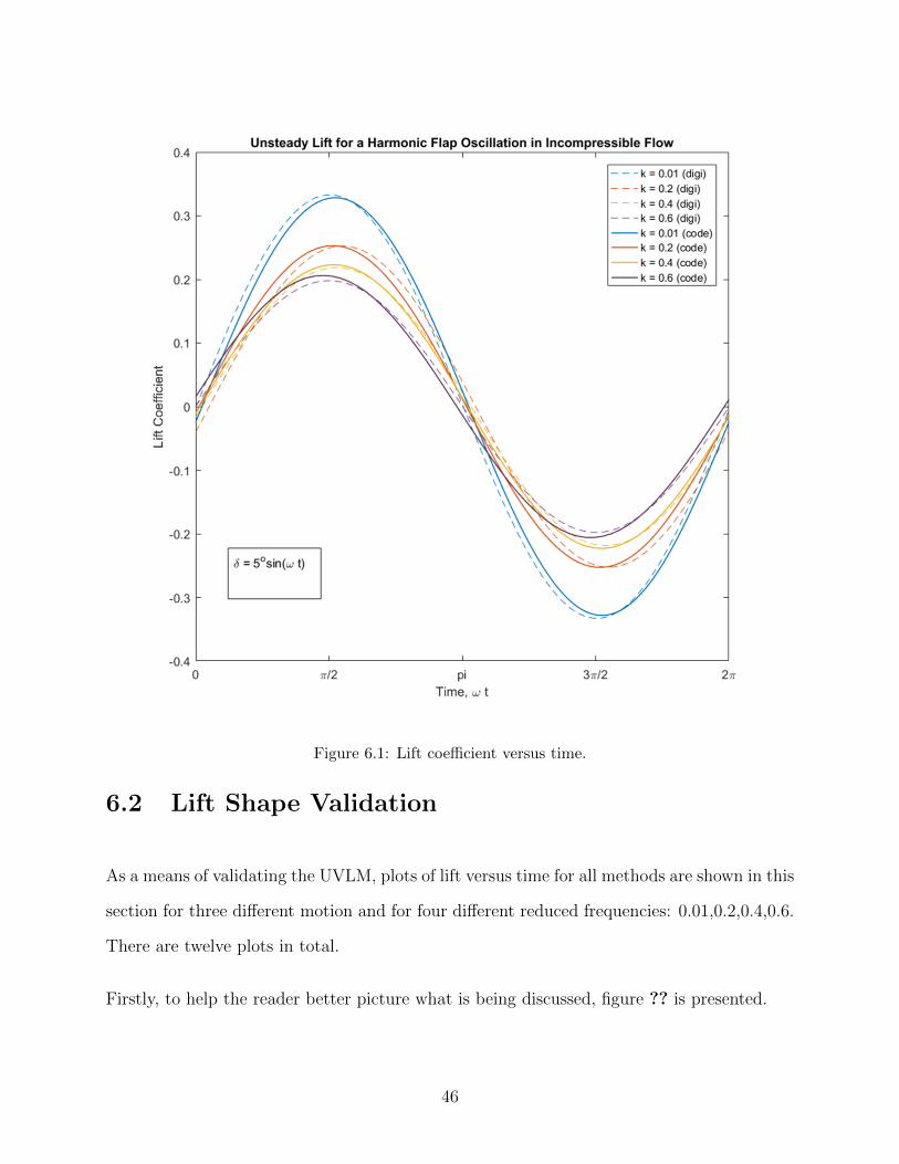
Figure 6.1: Lift coefficient versus time.

6.2 Lift Shape Validation

As a means of validating the UVLM, plots of lift versus time for all methods are shown in this

section for three different motion and for four different reduced frequencies: 0.01,0.2,0.4,0.6.

There are twelve plots in total.

Firstly, to help the reader better picture what is being discussed, figure ?? is presented.

46

Figure 6.2: A 2D visualization of an oscillatingflap deflection. The black is the flat plate with aflap; the cyan is the wake convection. This imageis from the UVLM mid-run.

With the image in mind, three subsections

are created to better organize the presenta-

tion of the twelve plots .

6.2.1 Plunging

The plots are presented in order of increasing

frequency, with the final plot in this subsec-

tion being the exception. At k = 0.01, the

amplitude is too small to allow much analy-

sis on the scale that 6.3 is held to. The scale

is set for comparative purposes only.

Though the scale is useful for comparison of

frequencies, it is not useful for comparison of

methods at the lowest frequecy. Therefore,

figure 6.7 is created, which is the same plot

as figure 6.3 but at a different scale. The lift

behavior at plunging frequency k = 0.01 can

be discerned at this level.

As is evident from figure 6.7, Leishman’s formulation does not seem to accurately predict

the lift at such low frequencies. This is an oddity. The reader is challenged to look into the

author’s code (found in the appendix) to find a mistake. Leishman’s paper seems to show

accurate lift predictions, though the code based on his paper does not—for extremely low

frequencies, that is.

47

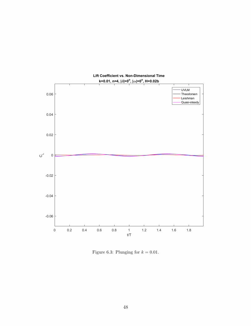
Figure 6.3: Plunging for k = 0.01.

48

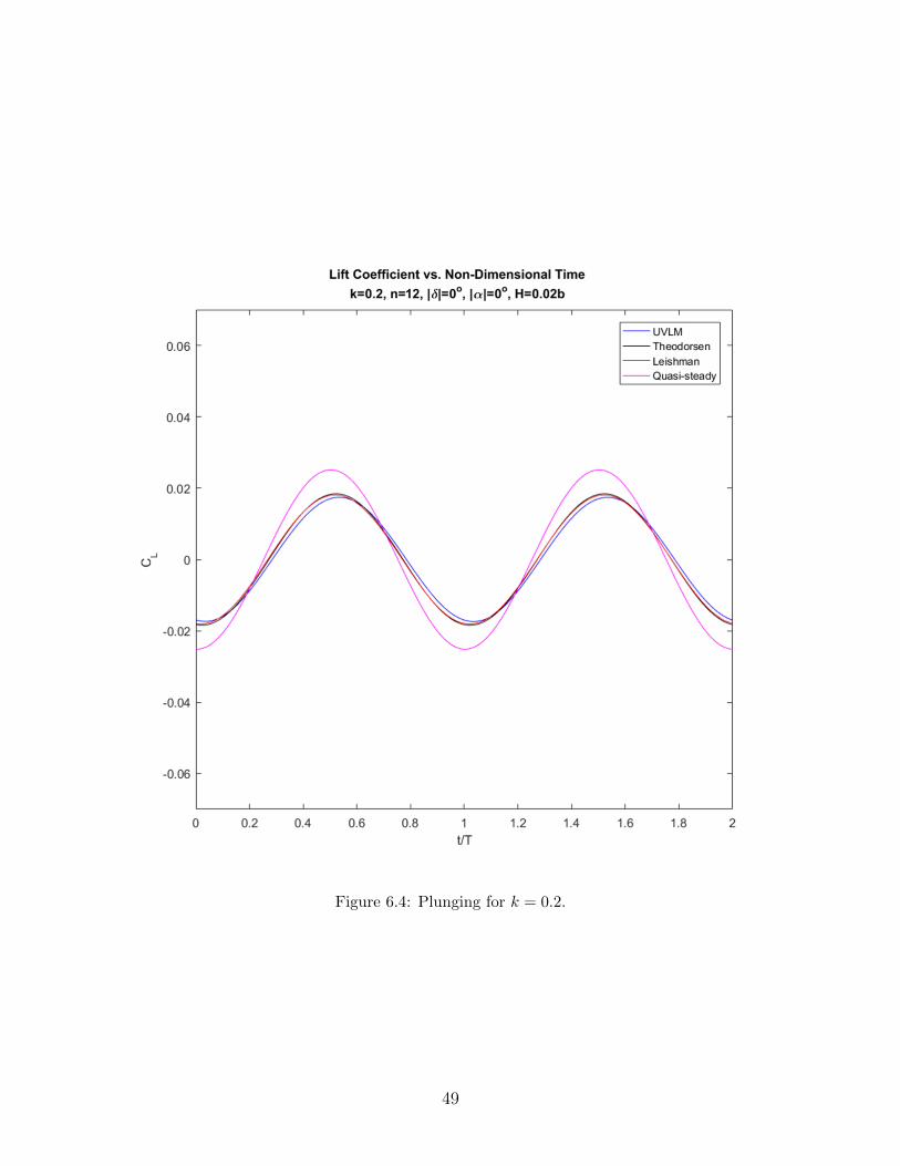
Figure 6.4: Plunging for k = 0.2.

49

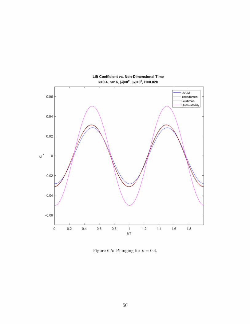
Figure 6.5: Plunging for k = 0.4.

50

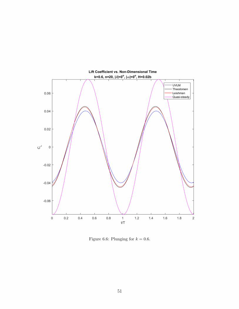
Figure 6.6: Plunging for k = 0.6.

51

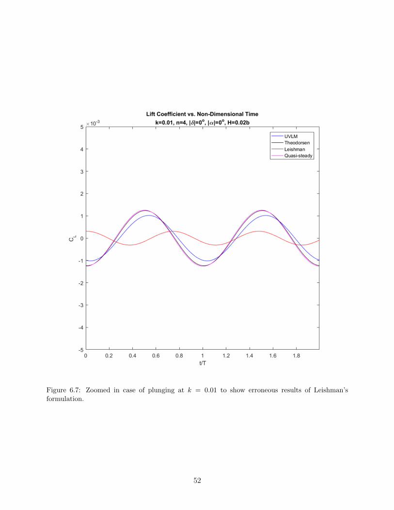
Figure 6.7: Zoomed in case of plunging at k = 0.01 to show erroneous results of Leishman’sformulation.

52

6.2.2 Pitching

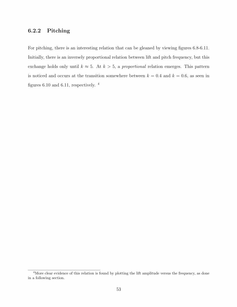
For pitching, there is an interesting relation that can be gleaned by viewing figures 6.8-6.11.

Initially, there is an inversely proportional relation between lift and pitch frequency, but this

exchange holds only until k ≈ 5. At k > 5, a proportional relation emerges. This pattern

is noticed and occurs at the transition somewhere between k = 0.4 and k = 0.6, as seen in

figures 6.10 and 6.11, respectively. 4

4More clear evidence of this relation is found by plotting the lift amplitude versus the frequency, as donein a following section.

53

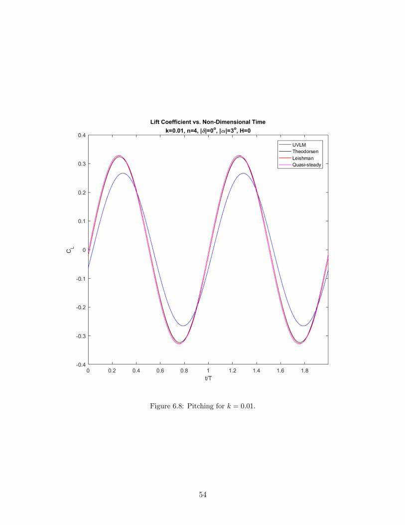
Figure 6.8: Pitching for k = 0.01.

54

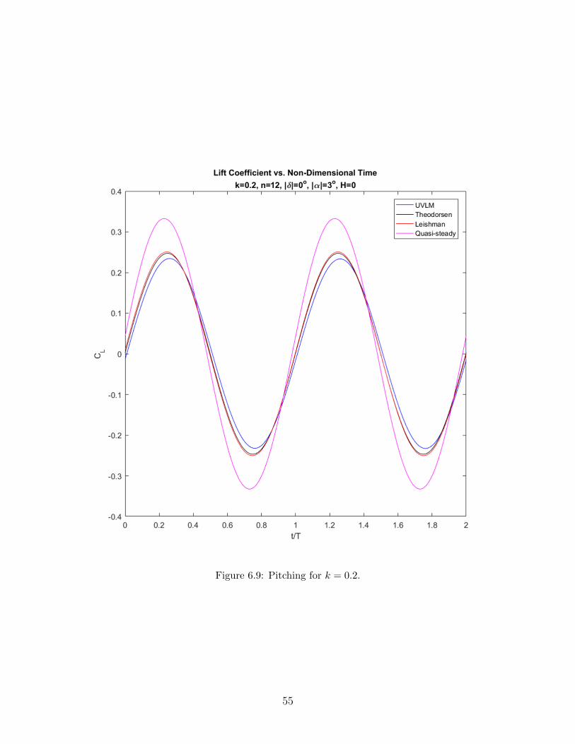
Figure 6.9: Pitching for k = 0.2.

55

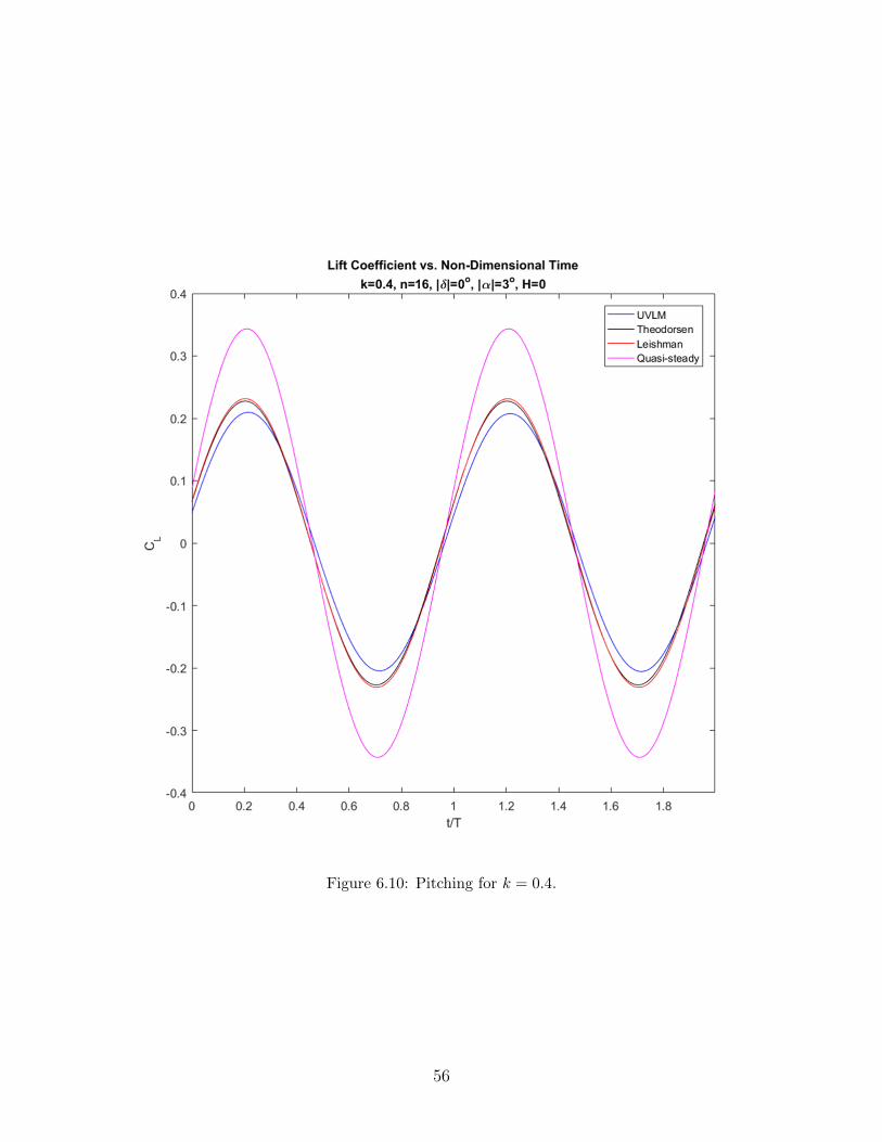
Figure 6.10: Pitching for k = 0.4.

56

Figure 6.11: Pitching for k = 0.6.

57

6.2.3 Flapping

Flapping exhibits a similar pattern to that of pitching, in that lift initially decreases with

increasing frequency until a certain transitional frequency is reached. At that value, which

here is between k = 1 and k = 2 5, the relation changes. Lift then increases proportionally

with frequency.

It should also be noted that Leishman’s plot for k = 0.01 is inaccurate, while for higher

frequencies Leishman is accurate when compared to Theodorsen’s. This is the same odd

tendency noticed for the pitching case.

Again, the reader is invited to check the author’s code if there exists any doubt about the

results.

5This is more clearly seen in a following section regarding lift amplitude.

58

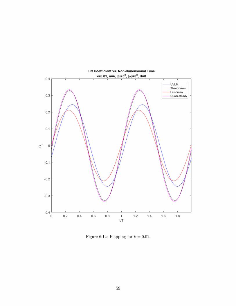
Figure 6.12: Flapping for k = 0.01.

59

Figure 6.13: Flapping for k = 0.2.

60

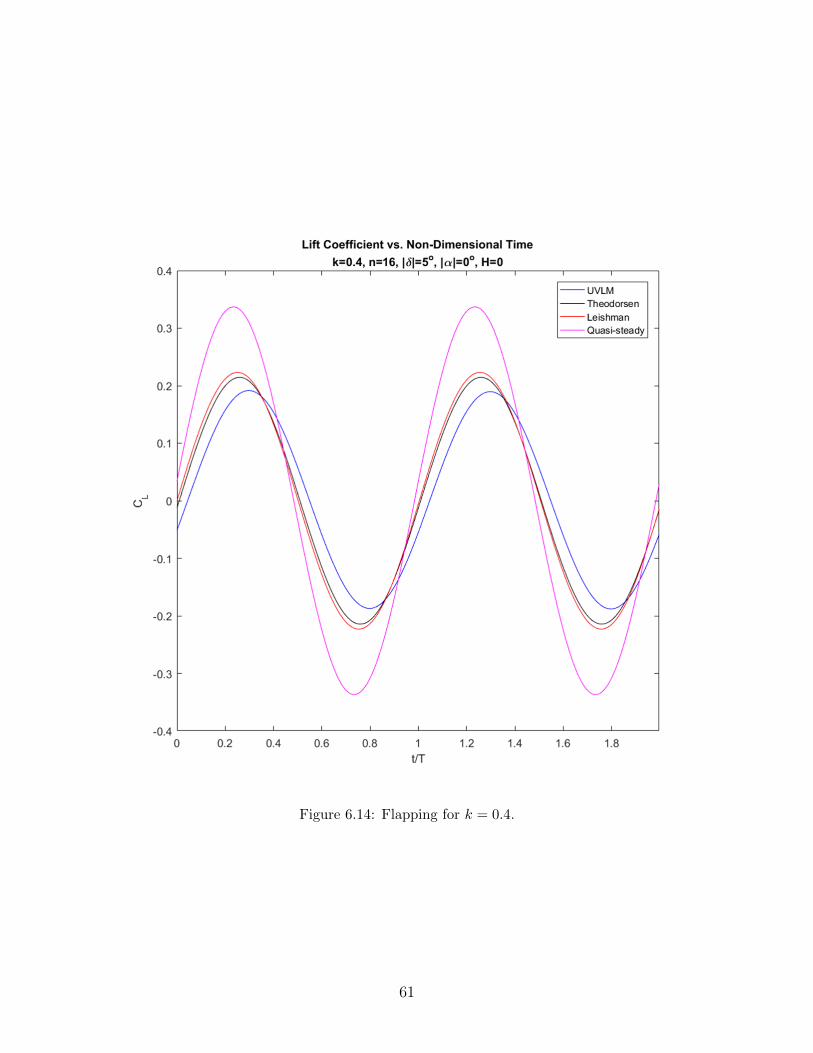
Figure 6.14: Flapping for k = 0.4.

61

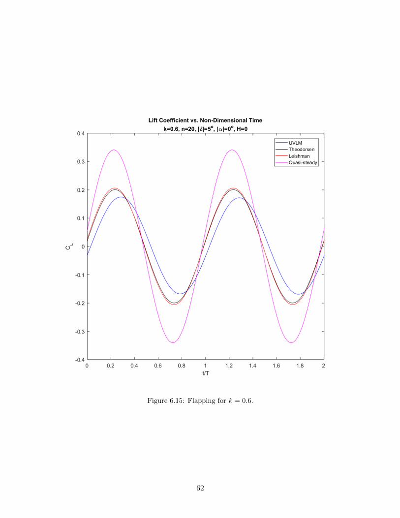
Figure 6.15: Flapping for k = 0.6.

62

Lift Shape Validation The plotting of lift for varying motions and frequencies demon-

strates a few interesting patterns, but the overall point of this section is to validate the

accuracy of the UVLM in predicting the output shape of the lift curve. As is seen by the

plots, the UVLM holds to the proper sinusoidal output when given an sinusoidal input, just

as the analytical methods. The UVLM, like Leishman, can also handle non-harmonic inputs

(unlike Theodorsen’s formulation), but a demonstration of that is not found in this paper.

6.3 Root-Mean Square Error

In order to establish the frequency range for which the select numerical method is accurate,

it is useful to investigate the root-mean square error (RMSe) of the lift coefficient as it varies

with the reduced frequency. The error is defined as

RMSe = 100%×

√∑Ti=1(CLUVLMi

− CLTheoi)

T(6.1)

where the T here denotes the final time step, and the argument in the square root is the

difference between the UVLM and Theodorsen formulations of lift.

Applying equation (6.1) to the plunging, pitching, and flapping results in the plot below.

As described by Robert J. S. Simpson[12], it is noted that, given a discretization, the UVLM

shows increasing discrepancies with analytical theory. However, using such knowledge, the

plot for figure 6.16 was generated using an increasingly dense set of collocation points in pro-

portion to an increase in reduced frequency. A quantitative relation between discretization

and frequency was not used, but a qualitative approach was.

Even so, it is clear by that the UVLM diverges from the analytical values in proportion to

the frequency. The motion of flapping generates a much higher degree of error than the other

63

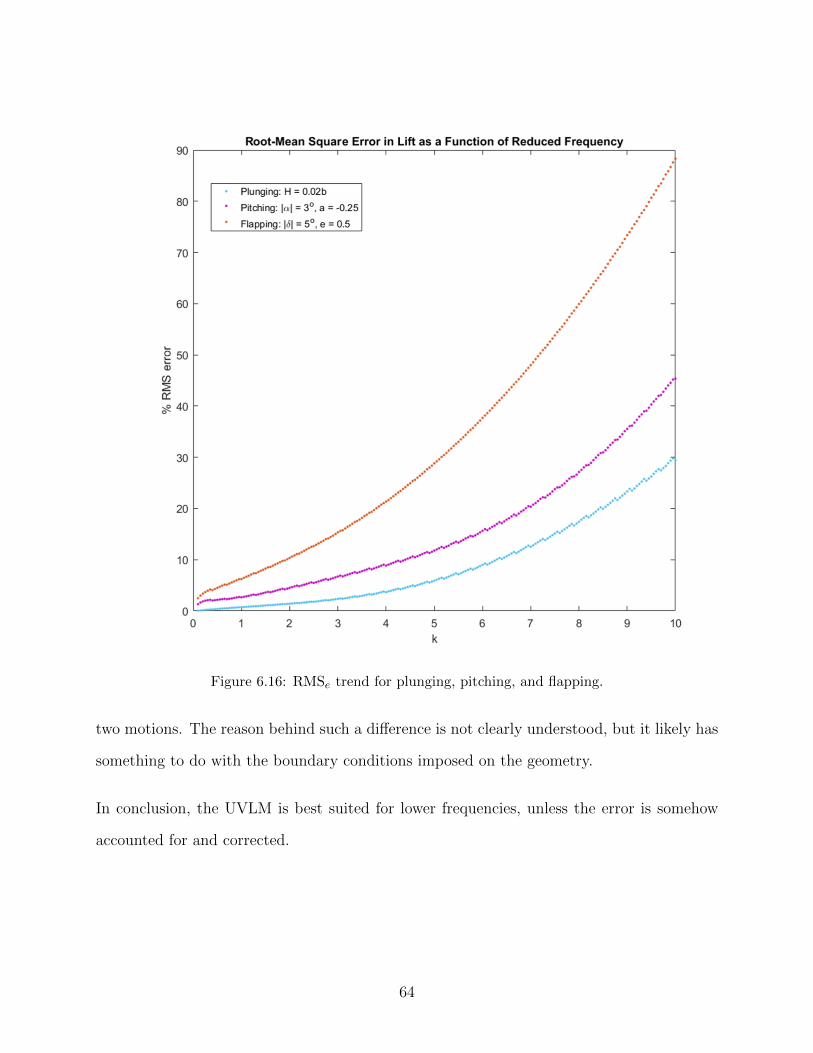
Figure 6.16: RMSe trend for plunging, pitching, and flapping.

two motions. The reason behind such a difference is not clearly understood, but it likely has

something to do with the boundary conditions imposed on the geometry.

In conclusion, the UVLM is best suited for lower frequencies, unless the error is somehow

accounted for and corrected.

64

6.4 Phase Difference

It is useful to investigate the effects frequency and kinematic motion have on the phase φ of

the unsteady lift with respect to the quasi-steady lift. There is a certain lag of the circulatory

lift that is intrinsic to the fluid, but geometric motion and frequency seem to play a role in

the degree of the that lag, as is shown in the below figures.

Figure 6.17: The phase difference φ for a plunging motion.

The general pattern noticed from figures 6.17-6.19 is that the phase difference φ is inversely

proportional to the frequency. In essence, the unsteady lift shifts from lagging behind the

65

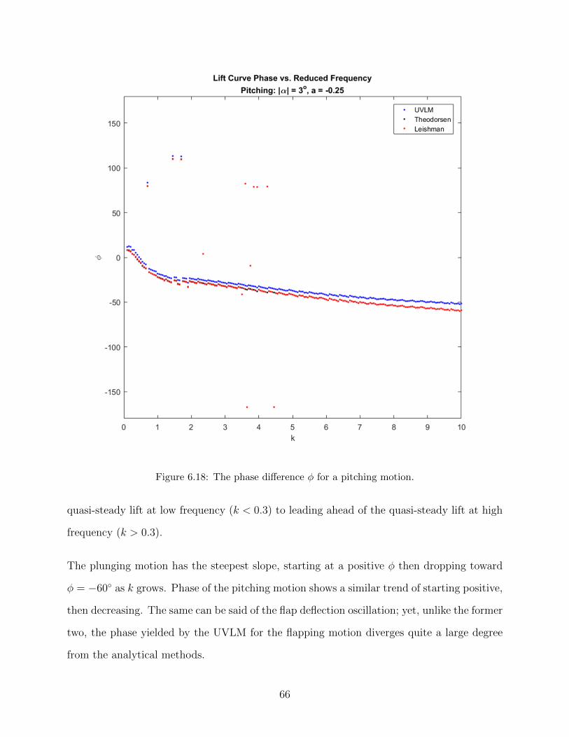
Figure 6.18: The phase difference φ for a pitching motion.

quasi-steady lift at low frequency (k < 0.3) to leading ahead of the quasi-steady lift at high

frequency (k > 0.3).

The plunging motion has the steepest slope, starting at a positive φ then dropping toward

φ = −60 as k grows. Phase of the pitching motion shows a similar trend of starting positive,

then decreasing. The same can be said of the flap deflection oscillation; yet, unlike the former

two, the phase yielded by the UVLM for the flapping motion diverges quite a large degree

from the analytical methods.

66

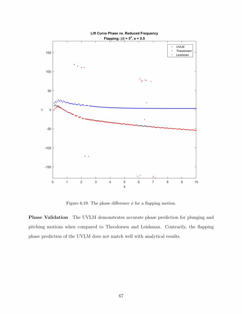
Figure 6.19: The phase difference φ for a flapping motion.

Phase Validation The UVLM demonstrates accurate phase prediction for plunging and

pitching motions when compared to Theodorsen and Leishman. Contrarily, the flapping

phase prediction of the UVLM does not match well with analytical results.

67

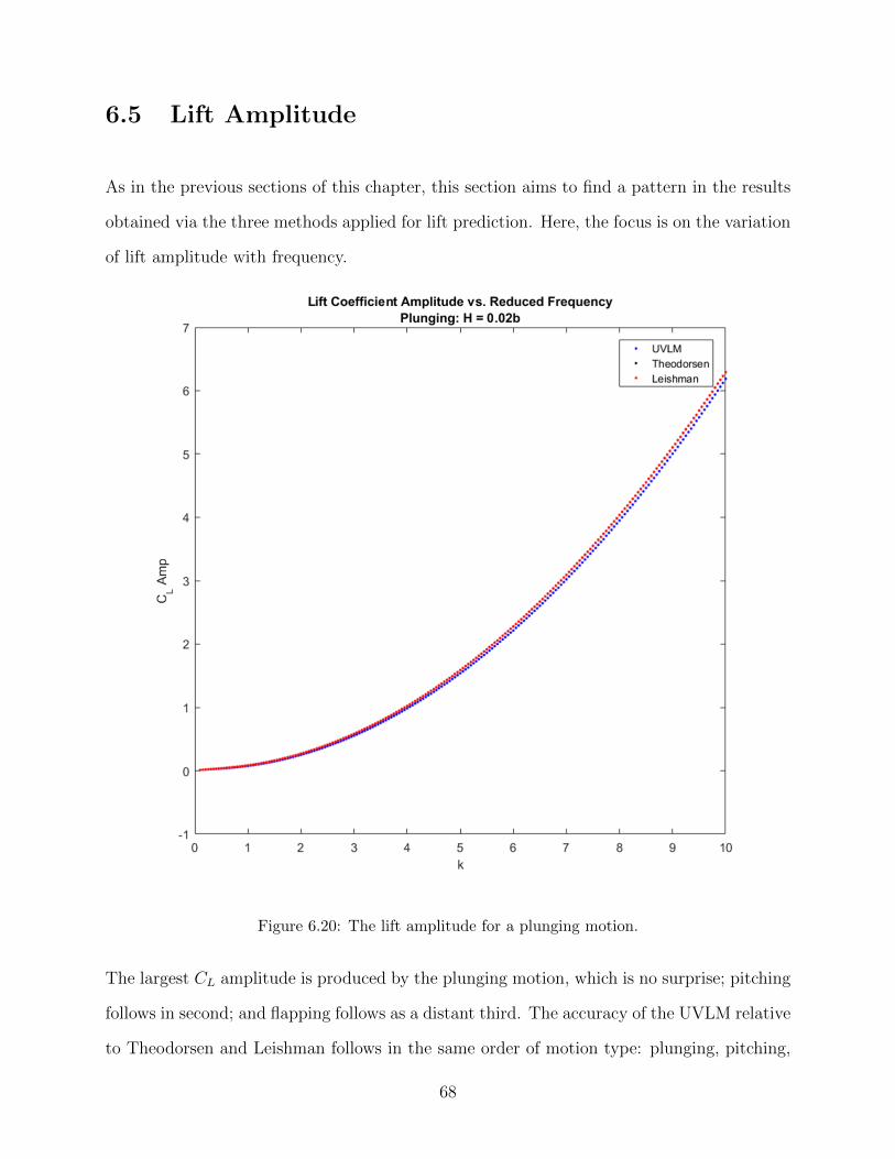
6.5 Lift Amplitude

As in the previous sections of this chapter, this section aims to find a pattern in the results

obtained via the three methods applied for lift prediction. Here, the focus is on the variation

of lift amplitude with frequency.

Figure 6.20: The lift amplitude for a plunging motion.

The largest CL amplitude is produced by the plunging motion, which is no surprise; pitching

follows in second; and flapping follows as a distant third. The accuracy of the UVLM relative

to Theodorsen and Leishman follows in the same order of motion type: plunging, pitching,

68

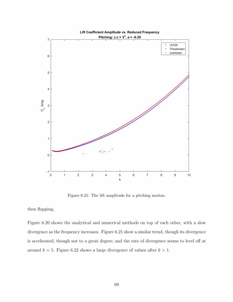
Figure 6.21: The lift amplitude for a pitching motion.

then flapping.

Figure 6.20 shows the analytical and numerical methods on top of each other, with a slow

divergence as the frequency increases. Figure 6.21 show a similar trend, though its divergence

is accelerated, though not to a great degree; and the rate of divergence seems to level off at

around k = 5. Figure 6.22 shows a large divergence of values after k > 1.

69

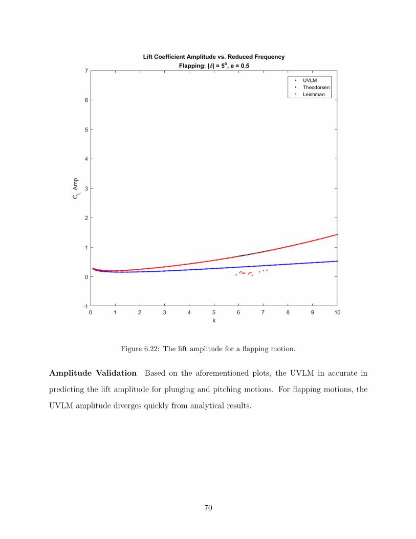
Figure 6.22: The lift amplitude for a flapping motion.

Amplitude Validation Based on the aforementioned plots, the UVLM in accurate in

predicting the lift amplitude for plunging and pitching motions. For flapping motions, the

UVLM amplitude diverges quickly from analytical results.

70

6.6 Mean Lift

The amplitude of the lift does not tell the full story; it says nothing in regard to whether or

not a net non-zero lift force is produced. But determining the mean lift does just that.

For the UVLM, the mean lift of the UVLM is calculated using the following equation.

CL =1

T

T∑k=1

CLk (6.2)

The mean function in MATLAB is used to calculate the mean of the analytical methods,

but for the numerical method it does not yield results as accurate as can be. Therefore,

equation 6.2 is used explicitly for UVLM calculations, which in turn produces smooth results

comparable to using mean for Theodorsen and Leishman.

Regarding the plots, a fifth order polynomial fit was to make the trend more easily recog-

nizable. The exact points on the

71

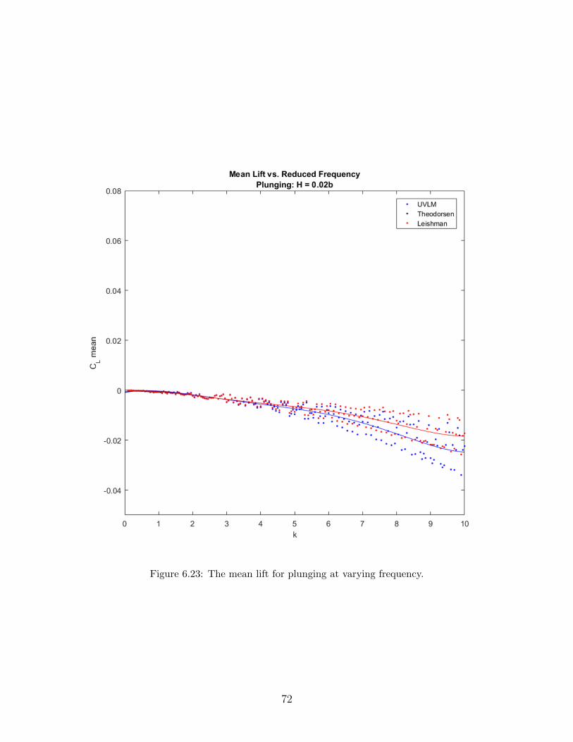
Figure 6.23: The mean lift for plunging at varying frequency.

72

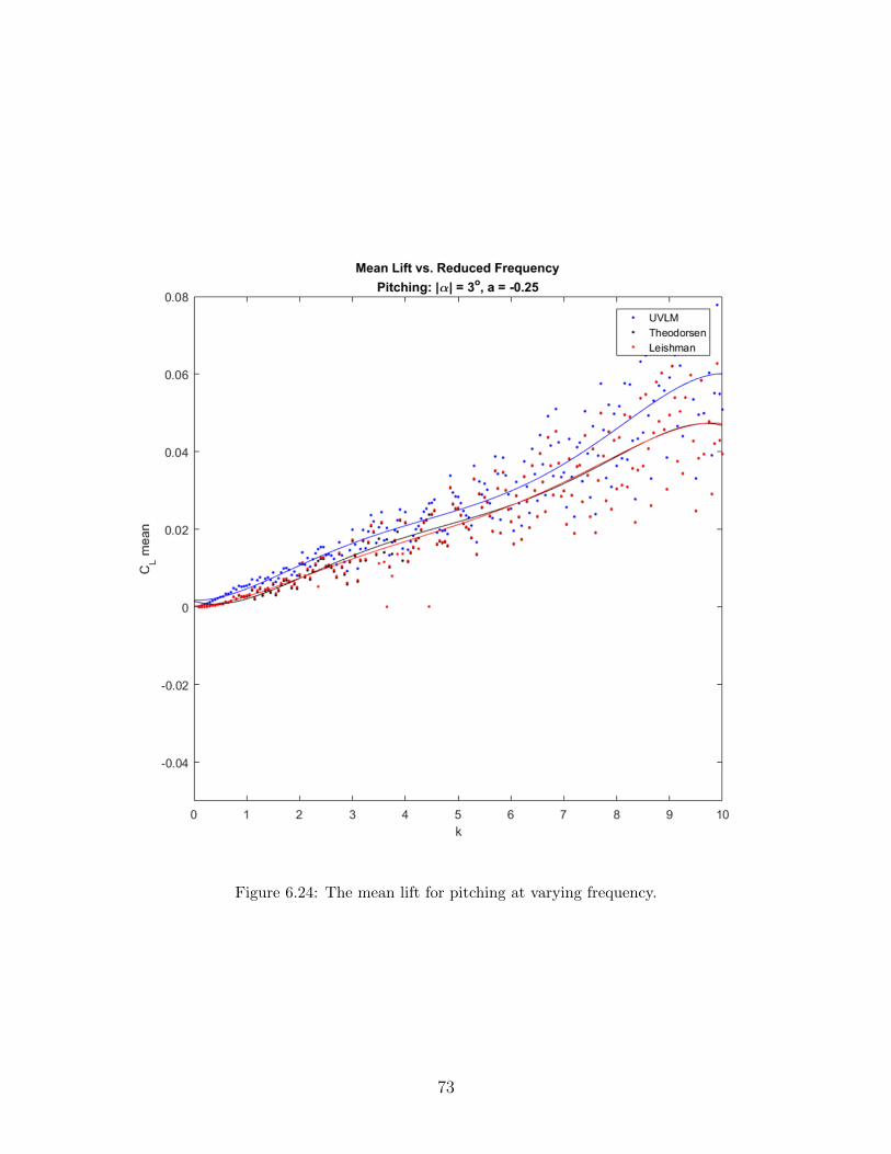
Figure 6.24: The mean lift for pitching at varying frequency.

73

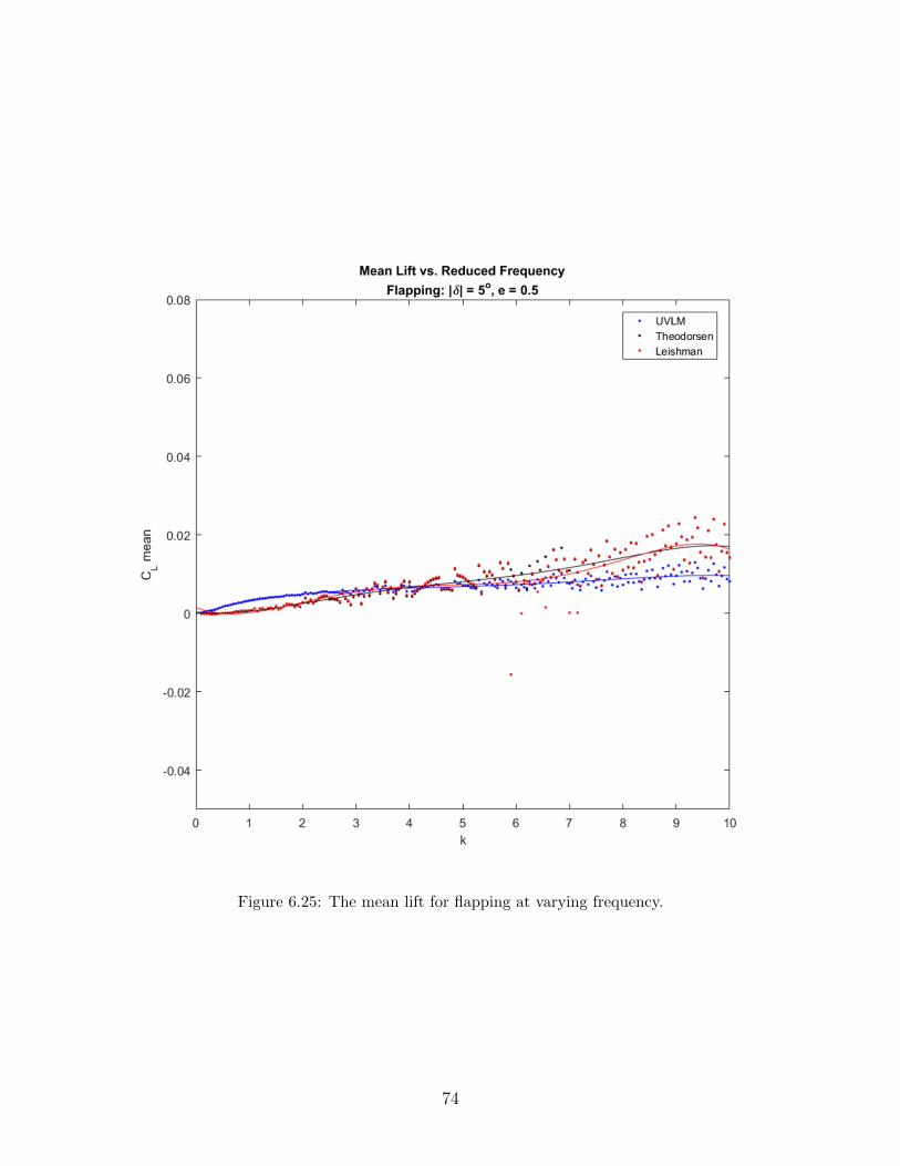
Figure 6.25: The mean lift for flapping at varying frequency.

74

Mean Lift Validation The plots for the mean lift are quite scattered. The CL values

vary in a seemingly random way as the frequency changes. It can be noted, however, that by

viewing the polynomial fit line the UVLM maintains a similar trend to that of the analytical

methods. Divergence occurs at high frequencies, which is the normal behavior of the select

numerical method.

75

Chapter 7

Conclusion and Future Work

7.1 Conclusion

This article addresses the general effects of time-dependent motions on the unsteady lift

response in potential flow for unsteady vortex lattice method (UVLM). Many things are

explored, and a summary of the results is given in the following paragraphs.

The UVLM outputs a signal representative of the input signal. For example, as seen in the

Lift Shape section, the output is sinusoidal for a given sinusoidal input. Unlike Theodorsen’s

formulation, the UVLM, like Leishman’s description, can handle inputs other than those

harmonic in nature. These, however, are not explored in this paper.

Regarding RMS error, it is shown that the error is proportional to frequency. The higher

the frequency, the greater degree to which the UVLM deviates from analytical models. It is

concluded, therefore, that the select numerical method be used for frequencies of k ≤ 1.

The phase difference φ of the UVLM lift against the quasi-steady lift is well in line with the

analytical methods for plunging and pitching motions of the parameters explored (H = 0.02b

76

and |α| = 3o at a = −0.25, respectively), but such accuracy is not true for the prescribed

flapping motion (|δ| = 5o). Flap deflection measured with the UVLM starts at a different

value than Theodorsen and Leishman, even at low k, and it diverges even further as k

increases. It is suggested that such patterns be considered if the UVLM is to be used to

phase-sensitive studies.

As for lift, the amplitude of the UVLM measures closely with the two analytical methods for

plunging and pitching. For flapping, the UVLMs amplitude measures closely up to k ≈ 1,

but it diverges for k > 1. This error in flapping is expected after examining the RMS, as

noted previously.

When examining the mean lift of the motions, it is seen that plunging CL decreases with

increasing frequency, pitching CL increase with increasing frequency, and flapping CL shares

the same trend as pitching, though the slope is much smaller. The most effective lift-

producing motion of those prescribed is pitching.

In conclusion, the degree to which the UVLM matches with analytical results depends on

motion type and frequency. Regarding frequency, lower frequency tends to lead to the least

amount of error; and, as for motion, plunging has a smaller error margin than either pitching

or flapping.

7.2 Future Work

7.2.1 Two-Dimensional

The present paper has tended to the analytical and numerical approach of lift response in-

duced by a two-dimensional airfoil with an oscillating flap in unsteady flow. One area of

research has been left out: experimental. Further investigation of the lift response to a sinu-

77

soidal input must be confronted through experimentation. The author hopes to collaborate

with a colleague to tackle this particular endeavor.

The purpose of combining analytical, numerical, and experimental results is to eventually

develop a reduced-order model of aerodynamic phenomena. From this model, the author

plans to exploit the tools of geometric control in order to predict unintuitive effects of

various combinations of pitching, plunging, and flapping airfoils, with the main goal of using

unconventional means to increase lift or decrease drag for fighter aircraft maneuvers.

7.2.2 Three-Dimensional

Beyond the two-dimensional numerical approach, there is the more accurate three-dimensional

approach. Though adding an extra dimension increases the computational effort, the results

are more practical. The UVLM used in this paper can be extended to a third dimension,

though not without any lack of complexity. The author has already made attempts to write

the code and currently has preliminary—albeit inaccurate—results.

The erroneous results will not be put into this paper, but a figure of the visualization of a

single 3D UVLM run is below.

It is the author’s hope to perfect the 3D UVLM code, then exaggerate the aspect ratio in or-

der to validate it against a 2D analytical method. Of course, a comparison with experimental

data is also desired, but that will not be the first mode of validation.

Following aerodynamic validation, the 3D UVLM will ideally be combined with a structural

model to mimick phenomena other than those exhibited by rigid bodies.

78

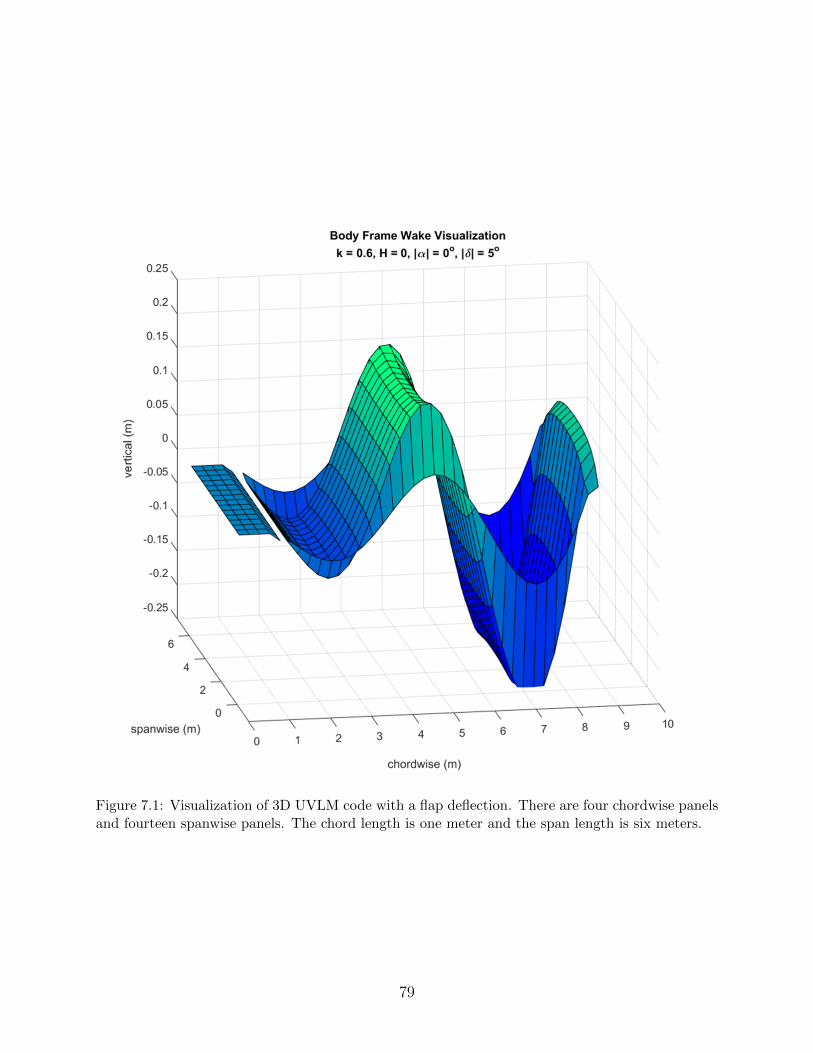
Figure 7.1: Visualization of 3D UVLM code with a flap deflection. There are four chordwise panelsand fourteen spanwise panels. The chord length is one meter and the span length is six meters.

79

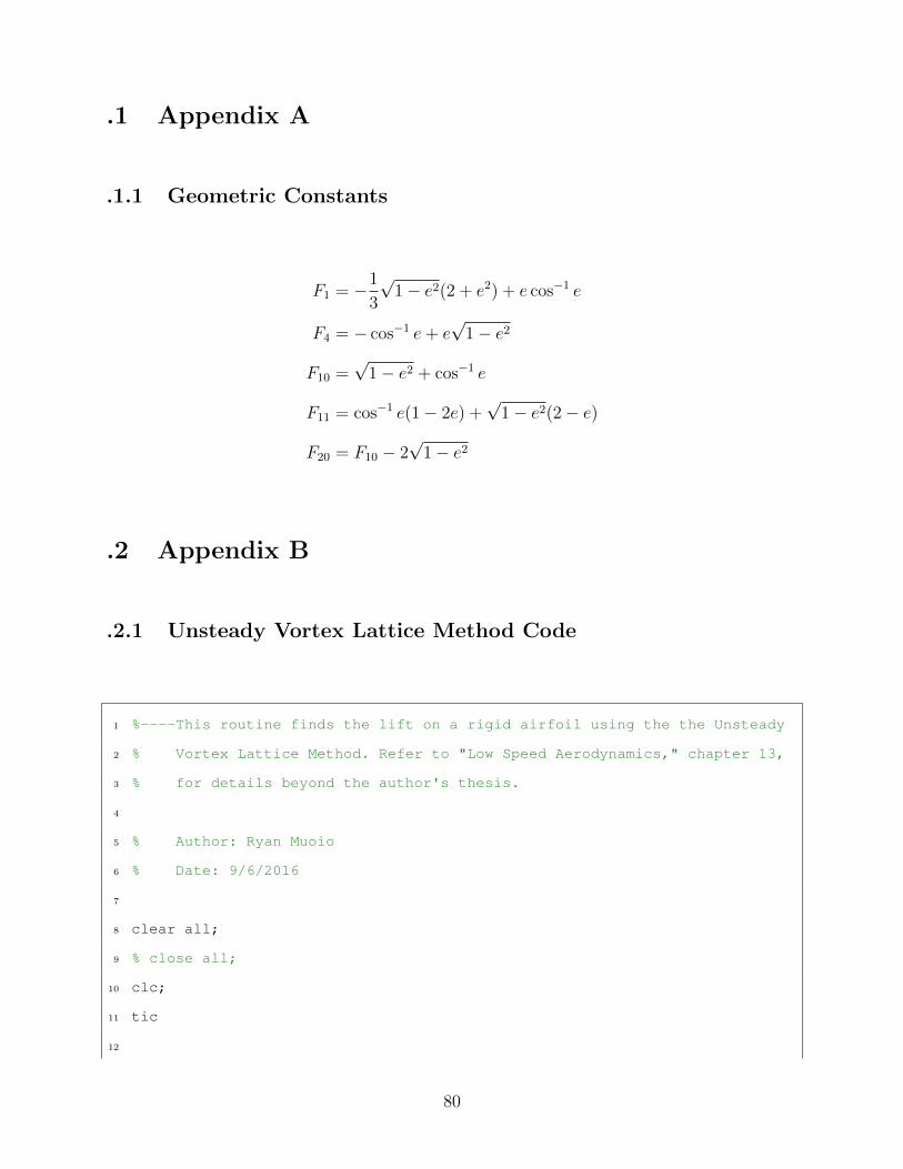
.1 Appendix A

.1.1 Geometric Constants

F1 = −1

3

√1− e2(2 + e2) + e cos−1 e

F4 = − cos−1 e+ e√

1− e2

F10 =√

1− e2 + cos−1 e

F11 = cos−1 e(1− 2e) +√

1− e2(2− e)

F20 = F10 − 2√

1− e2

.2 Appendix B

.2.1 Unsteady Vortex Lattice Method Code

1 %----This routine finds the lift on a rigid airfoil using the the Unsteady

2 % Vortex Lattice Method. Refer to "Low Speed Aerodynamics," chapter 13,

3 % for details beyond the author's thesis.

4

5 % Author: Ryan Muoio

6 % Date: 9/6/2016

7

8 clear all;

9 % close all;

10 clc;

11 tic

12

80

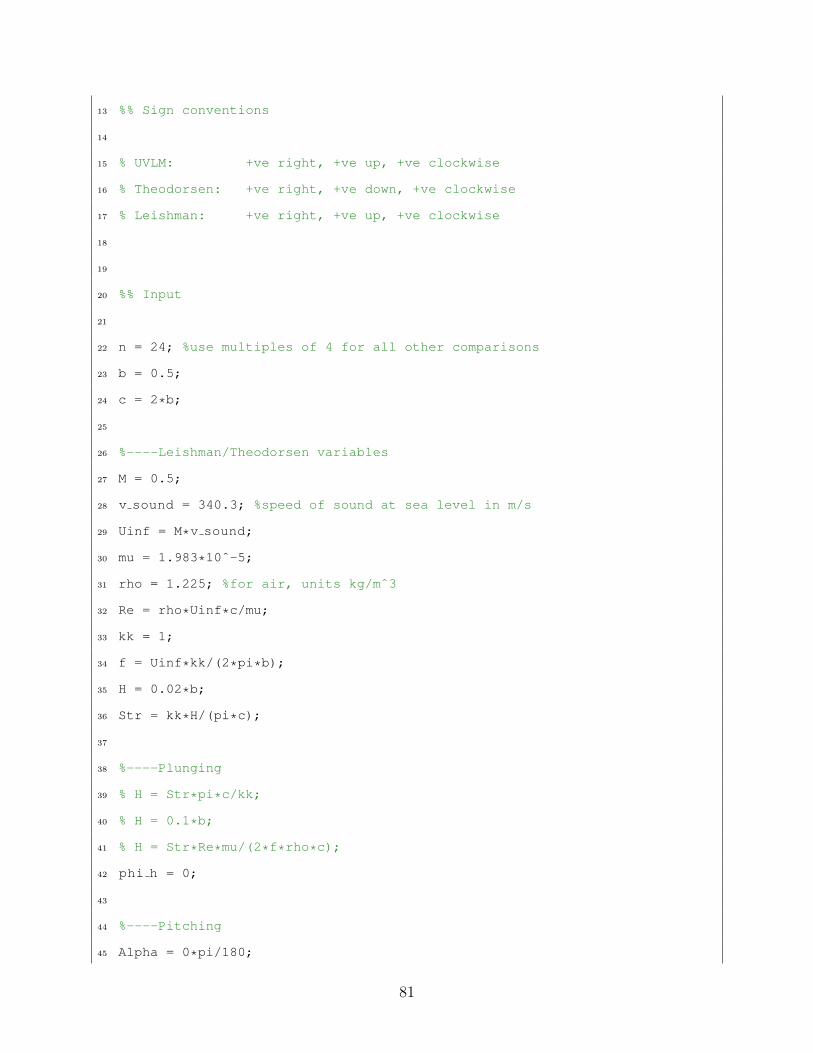
13 %% Sign conventions

14

15 % UVLM: +ve right, +ve up, +ve clockwise

16 % Theodorsen: +ve right, +ve down, +ve clockwise

17 % Leishman: +ve right, +ve up, +ve clockwise

18

19

20 %% Input

21

22 n = 24; %use multiples of 4 for all other comparisons

23 b = 0.5;

24 c = 2*b;

25

26 %----Leishman/Theodorsen variables

27 M = 0.5;

28 v sound = 340.3; %speed of sound at sea level in m/s

29 Uinf = M*v sound;

30 mu = 1.983*10ˆ-5;

31 rho = 1.225; %for air, units kg/mˆ3

32 Re = rho*Uinf*c/mu;

33 kk = 1;

34 f = Uinf*kk/(2*pi*b);

35 H = 0.02*b;

36 Str = kk*H/(pi*c);

37

38 %----Plunging

39 % H = Str*pi*c/kk;

40 % H = 0.1*b;

41 % H = Str*Re*mu/(2*f*rho*c);

42 phi h = 0;

43

44 %----Pitching

45 Alpha = 0*pi/180;

81

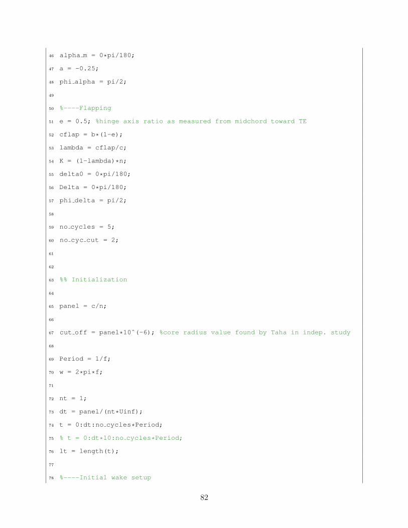
46 alpha m = 0*pi/180;

47 a = -0.25;

48 phi alpha = pi/2;

49

50 %----Flapping

51 e = 0.5; %hinge axis ratio as measured from midchord toward TE

52 cflap = b*(1-e);

53 lambda = cflap/c;

54 K = (1-lambda)*n;

55 delta0 = 0*pi/180;

56 Delta = 0*pi/180;

57 phi delta = pi/2;

58

59 no cycles = 5;

60 no cyc cut = 2;

61

62

63 %% Initialization

64

65 panel = c/n;

66

67 cut off = panel*10ˆ(-6); %core radius value found by Taha in indep. study

68

69 Period = 1/f;

70 w = 2*pi*f;

71

72 nt = 1;

73 dt = panel/(nt*Uinf);

74 t = 0:dt:no cycles*Period;

75 % t = 0:dt*10:no cycles*Period;

76 lt = length(t);

77

78 %----Initial wake setup

82

79 G = zeros(n+1,1);

80 G Wake = 0; %sum of wake vortices

81 no Wake = 0;

82 xz Wake = []; %position of wake vortices

83 G tot old = 0;

84

85

86 %% Pre-Allocation

87

88 %----UVLM

89 xz bound=zeros(n+1,2); xz cp=zeros(n,2); Nvec=zeros(n,2); Tvec=zeros(n,2);

90 hdot=zeros(lt,1); hdot2=zeros(lt,1); alpha=zeros(lt,1);

91 alphadot=zeros(lt,1); alphadot2=zeros(lt,1); delta=zeros(lt,1);

92 deltadot=zeros(lt,1); deltadot2=zeros(lt,1);

93 RHS=zeros(n+1,1); A=zeros(n+1,n+1); p diff=zeros(1,n);

94 Cp diff=zeros(1,n); Cl=zeros(1,lt); D=zeros(1,lt); P=zeros(1,lt);

95 CP UVLM=zeros(1,lt); Thrust UVLM=zeros(1,lt); CT UVLM=zeros(1,lt);

96 eta UVLM=zeros(1,lt); CD UVLM=zeros(1,lt); Cl avg=zeros(1,lt);

97

98

99 %% Time-Invariant Geometry

100

101 for i = 1:K

102 xz bound(i,1) = (i-1+0.25)*c/n;

103 xz bound(i,2) = 0;

104 xz cp(i,1) = (i-1+0.75)*c/n;

105 xz cp(i,2) = 0;

106 Nvec(i,[1 2]) = [0 1];

107 Tvec(i,[1 2]) = [1 0];

108 end

109

110

111 %% Time Loop

83

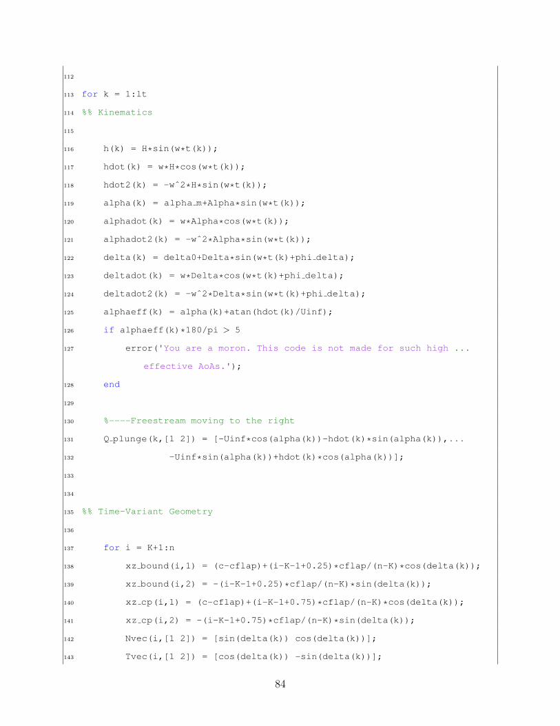
112

113 for k = 1:lt

114 %% Kinematics

115

116 h(k) = H*sin(w*t(k));

117 hdot(k) = w*H*cos(w*t(k));

118 hdot2(k) = -wˆ2*H*sin(w*t(k));

119 alpha(k) = alpha m+Alpha*sin(w*t(k));

120 alphadot(k) = w*Alpha*cos(w*t(k));

121 alphadot2(k) = -wˆ2*Alpha*sin(w*t(k));

122 delta(k) = delta0+Delta*sin(w*t(k)+phi delta);

123 deltadot(k) = w*Delta*cos(w*t(k)+phi delta);

124 deltadot2(k) = -wˆ2*Delta*sin(w*t(k)+phi delta);

125 alphaeff(k) = alpha(k)+atan(hdot(k)/Uinf);

126 if alphaeff(k)*180/pi > 5

127 error('You are a moron. This code is not made for such high ...

effective AoAs.');

128 end

129

130 %----Freestream moving to the right

131 Q plunge(k,[1 2]) = [-Uinf*cos(alpha(k))-hdot(k)*sin(alpha(k)),...

132 -Uinf*sin(alpha(k))+hdot(k)*cos(alpha(k))];

133

134

135 %% Time-Variant Geometry

136

137 for i = K+1:n

138 xz bound(i,1) = (c-cflap)+(i-K-1+0.25)*cflap/(n-K)*cos(delta(k));

139 xz bound(i,2) = -(i-K-1+0.25)*cflap/(n-K)*sin(delta(k));

140 xz cp(i,1) = (c-cflap)+(i-K-1+0.75)*cflap/(n-K)*cos(delta(k));

141 xz cp(i,2) = -(i-K-1+0.75)*cflap/(n-K)*sin(delta(k));

142 Nvec(i,[1 2]) = [sin(delta(k)) cos(delta(k))];

143 Tvec(i,[1 2]) = [cos(delta(k)) -sin(delta(k))];

84

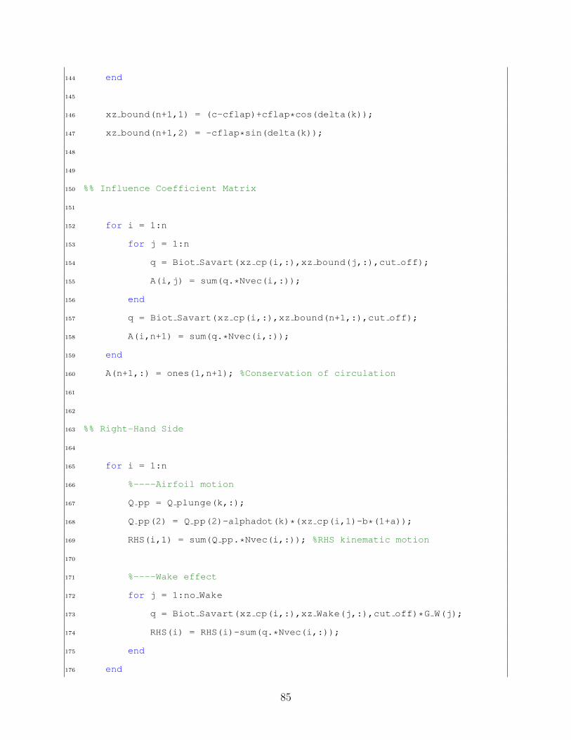
144 end

145

146 xz bound(n+1,1) = (c-cflap)+cflap*cos(delta(k));

147 xz bound(n+1,2) = -cflap*sin(delta(k));

148

149

150 %% Influence Coefficient Matrix

151

152 for i = 1:n

153 for j = 1:n

154 q = Biot Savart(xz cp(i,:),xz bound(j,:),cut off);

155 A(i,j) = sum(q.*Nvec(i,:));

156 end

157 q = Biot Savart(xz cp(i,:),xz bound(n+1,:),cut off);

158 A(i,n+1) = sum(q.*Nvec(i,:));

159 end

160 A(n+1,:) = ones(1,n+1); %Conservation of circulation

161

162

163 %% Right-Hand Side

164

165 for i = 1:n

166 %----Airfoil motion

167 Q pp = Q plunge(k,:);

168 Q pp(2) = Q pp(2)-alphadot(k)*(xz cp(i,1)-b*(1+a));

169 RHS(i,1) = sum(Q pp.*Nvec(i,:)); %RHS kinematic motion

170

171 %----Wake effect

172 for j = 1:no Wake

173 q = Biot Savart(xz cp(i,:),xz Wake(j,:),cut off)*G W(j);

174 RHS(i) = RHS(i)-sum(q.*Nvec(i,:));

175 end

176 end

85

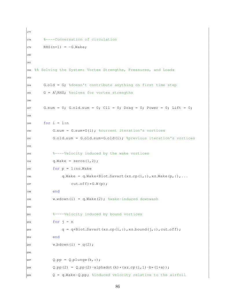
177

178 %----Conversation of circulation

179 RHS(n+1) = -G Wake;

180

181

182 %% Solving the System: Vortex Strengths, Pressures, and Loads

183

184 G old = G; %doesn't contribute anything on first time step

185 G = A\RHS; %solves for vortex strengths

186

187 G sum = 0; G old sum = 0; Cll = 0; Drag = 0; Power = 0; Lift = 0;

188

189 for i = 1:n

190 G sum = G sum+G(i); %current iteration's vortices

191 G old sum = G old sum+G old(i); %previous iteration's vortices

192

193 %----Velocity induced by the wake vortices

194 q Wake = zeros(1,2);

195 for p = 1:no Wake

196 q Wake = q Wake+Biot Savart(xz cp(i,:),xz Wake(p,:),...

197 cut off)*G W(p);

198 end

199 w wdown(i) = q Wake(2); %wake-induced downwash

200

201 %----Velocity induced by bound vortices

202 for j = n

203 q = q+Biot Savart(xz cp(i,:),xz bound(j,:),cut off);

204 end

205 w bdown(i) = q(2);

206

207 Q pp = Q plunge(k,:);

208 Q pp(2) = Q pp(2)-alphadot(k)*(xz cp(i,1)-b*(1+a));

209 Q = q Wake-Q pp; %induced velocity relative to the airfoil

86

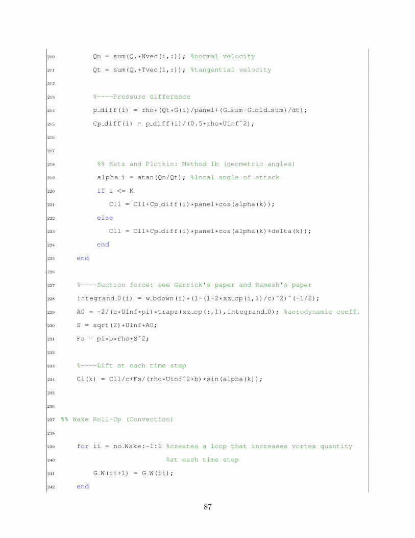
210 Qn = sum(Q.*Nvec(i,:)); %normal velocity

211 Qt = sum(Q.*Tvec(i,:)); %tangential velocity

212

213 %----Pressure difference

214 p diff(i) = rho*(Qt*G(i)/panel+(G sum-G old sum)/dt);

215 Cp diff(i) = p diff(i)/(0.5*rho*Uinfˆ2);

216

217

218 %% Katz and Plotkin: Method 1b (geometric angles)

219 alpha i = atan(Qn/Qt); %local angle of attack

220 if i <= K

221 Cll = Cll+Cp diff(i)*panel*cos(alpha(k));

222 else

223 Cll = Cll+Cp diff(i)*panel*cos(alpha(k)+delta(k));

224 end

225 end

226

227 %----Suction force: see Garrick's paper and Ramesh's paper

228 integrand 0(i) = w bdown(i)*(1-(1-2*xz cp(i,1)/c)ˆ2)ˆ(-1/2);

229 A0 = -2/(c*Uinf*pi)*trapz(xz cp(:,1),integrand 0); %aerodynamic coeff.

230 S = sqrt(2)*Uinf*A0;

231 Fs = pi*b*rho*Sˆ2;

232

233 %----Lift at each time step

234 Cl(k) = Cll/c+Fs/(rho*Uinfˆ2*b)*sin(alpha(k));

235

236

237 %% Wake Roll-Up (Convection)

238

239 for ii = no Wake:-1:1 %creates a loop that increases vortex quantity

240 %at each time step

241 G W(ii+1) = G W(ii);

242 end

87

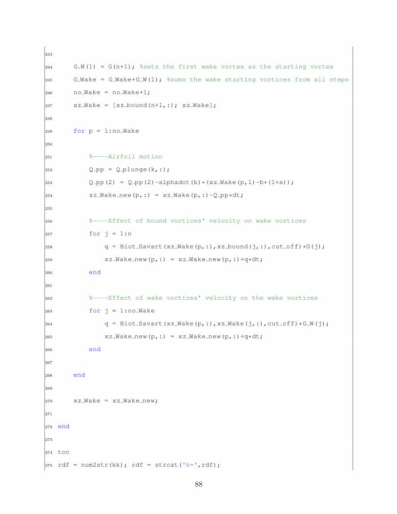
243

244 G W(1) = G(n+1); %sets the first wake vortex as the starting vortex

245 G Wake = G Wake+G W(1); %sums the wake starting vortices from all steps

246 no Wake = no Wake+1;

247 xz Wake = [xz bound(n+1,:); xz Wake];

248

249 for p = 1:no Wake

250

251 %----Airfoil motion

252 Q pp = Q plunge(k,:);

253 Q pp(2) = Q pp(2)-alphadot(k)*(xz Wake(p,1)-b*(1+a));

254 xz Wake new(p,:) = xz Wake(p,:)-Q pp*dt;

255

256 %----Effect of bound vortices' velocity on wake vortices

257 for j = 1:n

258 q = Biot Savart(xz Wake(p,:),xz bound(j,:),cut off)*G(j);

259 xz Wake new(p,:) = xz Wake new(p,:)+q*dt;

260 end

261

262 %----Effect of wake vortices' velocity on the wake vortices

263 for j = 1:no Wake

264 q = Biot Savart(xz Wake(p,:),xz Wake(j,:),cut off)*G W(j);

265 xz Wake new(p,:) = xz Wake new(p,:)+q*dt;

266 end

267

268 end

269

270 xz Wake = xz Wake new;

271

272 end

273

274 toc

275 rdf = num2str(kk); rdf = strcat('k=',rdf);

88

276 chord = num2str(c); chord = strcat('c=',chord);

277 panels = num2str(n); panels = strcat('n=',panels);

278 Reynolds = num2str(round(Re,-6)); Reynolds = strcat('Re=',Reynolds);

279 Strouhal = num2str(Str); Strouhal = strcat('St=',Strouhal);

280 FlapDef = num2str(Delta*180/pi); FlapDef = ...

strcat(' | \delta |=',FlapDef,'ˆo');

281 Pitch = num2str(Alpha*180/pi); Pitch = strcat(' | \alpha |=',Pitch,'ˆo');

282 Plunge = num2str(H); Plunge = strcat('H=',Plunge);

283

284 if no cyc cut ~= 0

285 Plotcut = round(no cyc cut/no cycles*lt); %removes transient cycles

286 Cl UVLM = Cl(Plotcut:lt);

287 Cl avg UVLM = Cl avg(Plotcut:lt);

288 CP UVLM = CP UVLM(Plotcut:lt);

289 eta UVLM = eta UVLM(Plotcut:lt);

290 t UVLM = t(Plotcut:lt);

291 delta UVLM = delta(Plotcut:lt);

292 Thrust UVLM = Thrust UVLM(Plotcut:lt);

293 CT UVLM = CT UVLM(Plotcut:lt);

294 CD UVLM = CD UVLM(Plotcut:lt);

295 alphaeff = alphaeff(Plotcut:lt);

296 end

297

298 %----Period-Averaged Propuslive Efficiency

299 eta avg = dt/((no cycles-no cyc cut)*Period)*sum(eta UVLM);

300 AvgEta = num2str(eta avg); AvgEta = strcat('\eta a=',AvgEta);

301

302 %----Period-Averaged Thrust Coefficient

303 CT Mean = dt/((no cycles-no cyc cut)*Period)*sum(CT UVLM);

304

305

306 %% Comparison with Theodorsen (Lift)

307 % Theodorsen: +ve right, +ve down, +ve clockwise

89

308

309 [Cl Theo,Cl Q Theo,T4,T10,C,QC,alpha,alphadot,alphadot2,Uinf,...

310 delta,deltadot,deltadot2,hdot2,L] = Theodorsen(b,rho,w,Uinf,H,Alpha,...

311 alpha m,a,e,delta0,Delta,kk,t,lt);

312

313 Cl Theo = Cl Theo(Plotcut:lt);

314 Cl Q Theo = Cl Q Theo(Plotcut:lt);

315 delta Theo = delta UVLM;

316 t Theo = t(Plotcut:lt);

317

318

319 %% Comparison with Leishman (Lift)

320 % Leishman: +ve right, +ve up, +ve clockwise

321

322 [Cl Leish,t,delta] = Leishman(t,e,H,Alpha,alpha m,delta0,Delta,a,b,c,...

323 Uinf,w);

324 delta Leish = delta;

325

326 %----Nonlinear fit to give a smoother graph

327 my func = @(beta,t) beta(1)*sin(beta(2)*t+beta(3));

328 amp = (max(Cl Leish)-min(Cl Leish))/2;

329 beta0 = [amp; w; 0];

330 beta = nlinfit(t,Cl Leish',my func,beta0);

331 t Leish = t UVLM;

332 Cl Leish = my func(beta,t Leish);

333

334

335 %% Root-Mean Square Error

336

337 for i = 1:length(t UVLM)

338 argument(i) = (Cl UVLM(i)-Cl Theo(i))ˆ2;

339 end

340 RMS = 100*sqrt(sum(argument)/length(t UVLM));

90

341

342

343 %% Amplitude & Phase Shift

344

345 AmpL UVLM = (max(Cl UVLM)-min(Cl UVLM))/2;

346 AmpL Theo = (max(Cl Theo)-min(Cl Theo))/2;

347 AmpL Leish = (max(Cl Leish)-min(Cl Leish))/2;

348

349 %----The phase differences are taken relative to the quasi-steady lift of

350 %Theodorsen.

351 PhaseD UVLM = Phase diff(Cl Q Theo,Cl UVLM);

352 PhaseD Theodorsen = Phase diff(Cl Q Theo,Cl Theo);

353 PhaseD Leishman = Phase diff(Cl Q Theo,Cl Leish);

.2.2 Theodorsen Code

1 function [Cl Theo,Cl Q Theo,T4,T10,C,QC,alpha,alphadot,alphadot2,Uinf,...

2 delta,deltadot,deltadot2,hdot2,L] = Theodorsen(b,rho,w,Uinf,H,Alpha,...

3 alpha m,a,e,delta0,Delta,kk,t,lt)

4

5 % H = -H; %changing sign convention to match Theodorsen's

6

7 %----Pre-Allocation

8 hdot=zeros(lt,1); hdot2=zeros(lt,1); alpha=zeros(lt,1);

9 alphadot=zeros(lt,1); alphadot2=zeros(lt,1); delta=zeros(lt,1);

10 deltadot=zeros(lt,1); deltadot2=zeros(lt,1);

11 hdotC=zeros(1,lt); alphaC=zeros(1,lt); alphadotC=zeros(1,lt);

12 deltaC=zeros(1,lt); deltadotC=zeros(1,lt);

13

14 %----Theodorsen Function

91

15 C = besselh(1,2,kk)/(besselh(1,2,kk)+1i*besselh(0,2,kk));

16 phi = angle(C);

17

18 %----Constants

19 T1 = -1/3*sqrt(1-eˆ2)*(2+eˆ2)+e*acos(e);

20 T4 = -acos(e)+e*sqrt(1-eˆ2);

21 T10 = sqrt(1-eˆ2)+acos(e);

22 T11 = acos(e)*(1-2*e)+sqrt(1-eˆ2)*(2-e);

23

24 if Alpha ~= 0

25 Alpha = -Alpha;

26 alpha m = -alpha m;

27 end

28 if Delta ~= 0

29 Delta = -Delta;

30 delta0 = -delta0;

31 end

32

33 for k = 1:lt

34

35 hdot(k) = w*H*cos(w*t(k));

36 hdot2(k) = -wˆ2*H*sin(w*t(k));

37 alpha(k) = alpha m+Alpha*sin(w*t(k));

38 alphadot(k) = w*Alpha*cos(w*t(k));

39 alphadot2(k) = -wˆ2*Alpha*sin(w*t(k));

40 delta(k) = delta0+Delta*sin(w*t(k));

41 deltadot(k) = w*Delta*cos(w*t(k));

42 deltadot2(k) = -wˆ2*Delta*sin(w*t(k));

43

44 %----Angles including the phase angle of the Theodorsen function

45 hdotC(k) = w*H*cos(w*t(k)+phi);

46 alphaC(k) = alpha m+Alpha*sin(w*t(k)+phi);

47 alphadotC(k) = w*Alpha*cos(w*t(k)+phi);

92

48 deltaC(k) = delta0+Delta*sin(w*t(k)+phi);

49 deltadotC(k) = w*Delta*cos(w*t(k)+phi);

50

51 %----Quasi-steady lift of Theordorsen

52 Q(k) = ...

-2*pi*rho*Uinf*b*(Uinf*alpha(k)+hdot(k)+b*(1/2-a)*alphadot(k)+...

53 T10/pi*Uinf*delta(k)+b/(2*pi)*T11*deltadot(k));

54 Cl Q Theo(k) = Q(k)/(rho*Uinfˆ2*b);

55

56 %----Quasi-steady with C(k) effect

57 QC(k) = Uinf*alphaC(k)+hdotC(k)+b*(1/2-a)*alphadotC(k)+...

58 T10/pi*Uinf*deltaC(k)+b/(2*pi)*T11*deltadotC(k);

59

60 %----Total lift on the airfoil-aileron system

61 L(k) = ...

-rho*bˆ2*(Uinf*pi*alphadot(k)+pi*hdot2(k)-pi*b*a*alphadot2(k)-Uinf*T4*...

62 deltadot(k)-T1*b*deltadot2(k))-2*pi*rho*Uinf*b*abs(C)*(QC(k));

63 Cl Theo(k) = L(k)/(rho*Uinfˆ2*b);

64

65 end

.2.3 Leishman Code

1 function [Cl Leish,t,delta] = Leishman(t,e,H,Alpha,alpha m,delta0,Delta,...

2 a,b,c,Uinf,w)

3

4 H = -H; %changing sign back to match Leishman's convention

5

6 %----Results from second-order step response approximation to Wagner's.

7 %A nonlinear least-squares fit using a constrained optimization

93

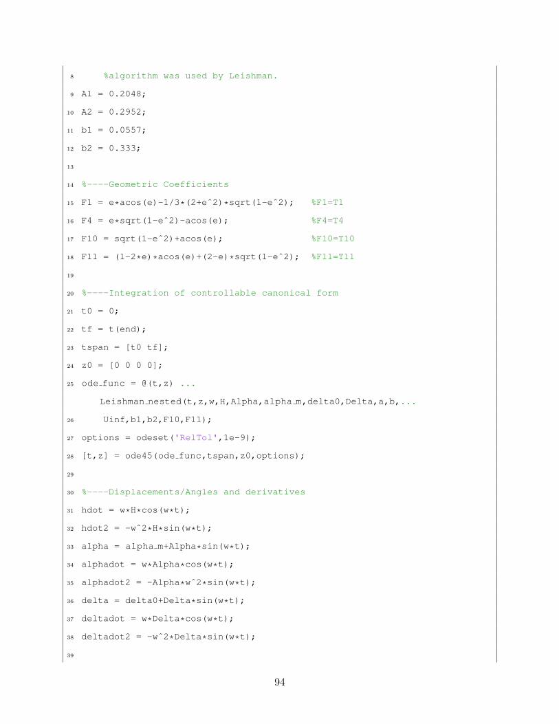
8 %algorithm was used by Leishman.

9 A1 = 0.2048;

10 A2 = 0.2952;

11 b1 = 0.0557;

12 b2 = 0.333;

13

14 %----Geometric Coefficients

15 F1 = e*acos(e)-1/3*(2+eˆ2)*sqrt(1-eˆ2); %F1=T1

16 F4 = e*sqrt(1-eˆ2)-acos(e); %F4=T4

17 F10 = sqrt(1-eˆ2)+acos(e); %F10=T10

18 F11 = (1-2*e)*acos(e)+(2-e)*sqrt(1-eˆ2); %F11=T11

19

20 %----Integration of controllable canonical form

21 t0 = 0;

22 tf = t(end);

23 tspan = [t0 tf];

24 z0 = [0 0 0 0];

25 ode func = @(t,z) ...

Leishman nested(t,z,w,H,Alpha,alpha m,delta0,Delta,a,b,...

26 Uinf,b1,b2,F10,F11);

27 options = odeset('RelTol',1e-9);

28 [t,z] = ode45(ode func,tspan,z0,options);

29

30 %----Displacements/Angles and derivatives

31 hdot = w*H*cos(w*t);

32 hdot2 = -wˆ2*H*sin(w*t);

33 alpha = alpha m+Alpha*sin(w*t);

34 alphadot = w*Alpha*cos(w*t);

35 alphadot2 = -Alpha*wˆ2*sin(w*t);

36 delta = delta0+Delta*sin(w*t);

37 deltadot = w*Delta*cos(w*t);

38 deltadot2 = -wˆ2*Delta*sin(w*t);

39

94

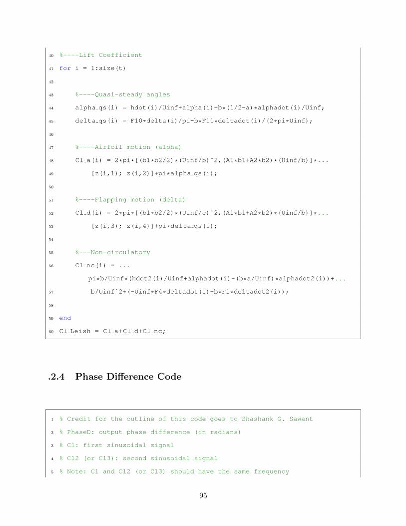
40 %----Lift Coefficient

41 for i = 1:size(t)

42

43 %----Quasi-steady angles

44 alpha qs(i) = hdot(i)/Uinf+alpha(i)+b*(1/2-a)*alphadot(i)/Uinf;

45 delta qs(i) = F10*delta(i)/pi+b*F11*deltadot(i)/(2*pi*Uinf);

46

47 %----Airfoil motion (alpha)

48 Cl a(i) = 2*pi*[(b1*b2/2)*(Uinf/b)ˆ2,(A1*b1+A2*b2)*(Uinf/b)]*...

49 [z(i,1); z(i,2)]+pi*alpha qs(i);

50

51 %----Flapping motion (delta)

52 Cl d(i) = 2*pi*[(b1*b2/2)*(Uinf/c)ˆ2,(A1*b1+A2*b2)*(Uinf/b)]*...

53 [z(i,3); z(i,4)]+pi*delta qs(i);

54

55 %---Non-circulatory

56 Cl nc(i) = ...

pi*b/Uinf*(hdot2(i)/Uinf+alphadot(i)-(b*a/Uinf)*alphadot2(i))+...

57 b/Uinfˆ2*(-Uinf*F4*deltadot(i)-b*F1*deltadot2(i));

58

59 end

60 Cl Leish = Cl a+Cl d+Cl nc;

.2.4 Phase Difference Code

1 % Credit for the outline of this code goes to Shashank G. Sawant

2 % PhaseD: output phase difference (in radians)

3 % Cl: first sinusoidal signal

4 % Cl2 (or Cl3): second sinusoidal signal

5 % Note: Cl and Cl2 (or Cl3) should have the same frequency

95

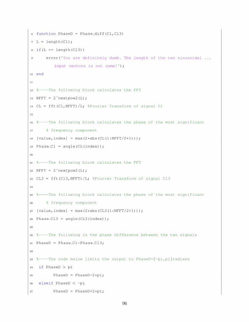
6 function PhaseD = Phase diff(Cl,Cl3)

7 L = length(Cl);

8 if(L ~= length(Cl3))

9 error('You are definitely dumb. The length of the two sinusoidal ...

input vectors is not same!');

10 end

11

12 %----The following block calculates the FFT

13 NFFT = 2ˆnextpow2(L);

14 CL = fft(Cl,NFFT)/L; %Fourier Transform of signal Cl

15

16 %----The following block calculates the phase of the most significant

17 % frequency component

18 [value,index] = max(2*abs(CL(1:NFFT/2+1)));

19 Phase Cl = angle(CL(index));

20

21 %----The following block calculates the FFT

22 NFFT = 2ˆnextpow2(L);

23 CL3 = fft(Cl3,NFFT)/L; %Fourier Transform of signal Cl3

24

25 %----The following block calculates the phase of the most significant

26 % frequency component

27 [value,index] = max(2*abs(CL3(1:NFFT/2+1)));

28 Phase Cl3 = angle(CL3(index));

29

30 %----The following is the phase difference between the two signals

31 PhaseD = Phase Cl-Phase Cl3;

32

33 %----The code below limits the output to PhaseD=-pi,piradians

34 if PhaseD > pi

35 PhaseD = PhaseD-2*pi;

36 elseif PhaseD < -pi

37 PhaseD = PhaseD+2*pi;

96

38 else

39 PhaseD = PhaseD;

40 end

41

42 return

43 end

97

References

[1] Theodore Theodorsen. General Theory of Aerodynamic Instability and the Mechanism of

Flutter. Technical Report NACA-TR-496, National Advisory Committee for Aeronautics.

Langley Aeronautical Lab., Langley Field, VA, United States, January 1935.

[2] I.E. Garrick. Propulsion of a Flapping and Oscillating Airfoil. Technical Report NACA-

TR-567, National Advisory Committee for Aeronautics. Langley Aeronautical Lab., Lan-

gley Field, VA, United States, January 1937.

[3] Wagner, Herbert: ’Uber die Entstehung des dynamischen Auftriebes von Tragfl’ugeln. Z.

f.a. M. M., Band 5, Heft 1, Feb. 1925,S. 17-35.

[4] von Karman, Th., and Burgers, J. M.: General Aerodynamic Theory—Perfect Fluids.

Aerodynamic Theory, W. F. Durand, ed., vol II, Julius Springer (Berlin), 1935.

[5] J. Gordon Leishman. Unsteady lift of a Flapped airfoil by Indicial Concepts. Journal of

Aircraft, 31(2):288-297, 1994.

[6] von Karman, Th., and Sears, W.R., ”Airfoil Theory for Non-Uniform Motion,” Journal

of the Aeronautical Sciences, Vol 5, No. 10, 1938, pp. 379-390.

[7] Jones, R.T, ”Calculation of the Motion of an Airplane Under the Influence of Irregular

Disturbances,” Journal of the Aeronautical Sciences, Vol 3, No. 12, 1936, pp. 419-425.

[8] Pistolesi, Enrico: Aerodinamica. Unione Tipografico—Editrice Torinese, 1932.

98

[9] Ramesh, Kiran, ”An Unsteady Airfoil Theory Applied to Pitching Motions Validated

Against Experiment and Computation,” Theoretical Computational Fluid Dynamics, 27,

843-864 (2013).

[10] Jones, R. T.,”Operational Treatment of the Non-Uniform Lift Theory in Airplane Dy-

namics.” 1938. Technical Note 667, NASA.

[11] Katz, J., and Plotkin, A., Low-Speed Aerodynamics, Cambridge Univ. Press, Cambridge,

England, U.K., 2001, pp. 369-447.

[12] Simpson, R. J. S., and Palacios, R, ”Induced-Drag Calculations in the Unsteady Vortex

Lattice Method,” AIAA Journal, Vol 51, No. 7, 2013, pp. 1775-1779.

99