Pitch control for ships with diesel mechanical and hybrid ...

Delft University of Technology

Pitch control for ships with diesel mechanical and hybrid propulsionModelling, validation and performance quantificationGeertsma, R. D.; Negenborn, R. R.; Visser, K.; Loonstijn, M. A.; Hopman, J. J.

DOI10.1016/j.apenergy.2017.09.103Publication date2017Document VersionFinal published versionPublished inApplied Energy

Citation (APA)Geertsma, R. D., Negenborn, R. R., Visser, K., Loonstijn, M. A., & Hopman, J. J. (2017). Pitch control forships with diesel mechanical and hybrid propulsion: Modelling, validation and performance quantification.Applied Energy, 206, 1609-1631. https://doi.org/10.1016/j.apenergy.2017.09.103

Important noteTo cite this publication, please use the final published version (if applicable).Please check the document version above.

CopyrightOther than for strictly personal use, it is not permitted to download, forward or distribute the text or part of it, without the consentof the author(s) and/or copyright holder(s), unless the work is under an open content license such as Creative Commons.

Takedown policyPlease contact us and provide details if you believe this document breaches copyrights.We will remove access to the work immediately and investigate your claim.

This work is downloaded from Delft University of Technology.For technical reasons the number of authors shown on this cover page is limited to a maximum of 10.

https://doi.org/10.1016/j.apenergy.2017.09.103

https://doi.org/10.1016/j.apenergy.2017.09.103

Contents lists available at ScienceDirect

Applied Energy

journal homepage: www.elsevier.com/locate/apenergy

Pitch control for ships with diesel mechanical and hybrid propulsion:Modelling, validation and performance quantification

R.D. Geertsmaa,b,⁎, R.R. Negenborna, K. Vissera,b, M.A. Loonstijna, J.J. Hopmana

a Department of Maritime & Transport Technology, Delft University of Technology, The Netherlandsb Faculty of Military Sciences, Netherlands Defence Academy, The Netherlands

H I G H L I G H T S

• A MVFP propulsion model for comparative ship and control system studies is proposed.

• Fuel consumption, acceleration, thermal loading & propeller cavitation are evaluated.

• Benchmark MOPs quantify these criteria within an hour simulation time.

• The propulsion model is validated with FAT and SAT data from a case study navy ship.

• Control can save 30% fuel, reduce thermal loading by 90 K and acceleration time by 50%.

A R T I C L E I N F O

Keywords:Mechanical propulsionNon-linear control systemsMarine systemsModelling and simulationValidationPower systems

A B S T R A C T

Ships, in particular service vessels, need to reduce fuel consumption, emissions and cavitation noise whilemaintaining manoeuvrability and preventing engine overloading. Diesel mechanical propulsion with con-trollable pitch propellers can provide high fuel efficiency with good manoeuvrability. However, the conventionalcontrol strategy with fixed combinator curves limits control freedom in trading-off performance characteristics.In order to evaluate performance of current state-of-the-art and future alternative propulsion systems and theircontrol, a validated propulsion system model is required. To this end, this paper proposes a propulsion modelwith a Mean Value First Principle (MVFP) diesel engine model that can be parameterised with publicly availablemanufacturer data and further calibrated with obligatory FAT measurements. The model uses a novel approachto predict turbocharger performance based on Zinner blowdown, the Büchi power and flow balance and theelliptic law for turbines, and does not require detailed information such as compressor and turbine maps. Thismodel predicts system performance within 5% of actual measurements during Factory Acceptance Tests (FAT) ofthe diesel engines and Sea Acceptance Tests (SAT) of a case study navy ship. Moreover, this paper proposesmeasures of performance that objectively quantify the fuel consumption, acceleration rate, engine thermalloading and propeller cavitation during trial, design and off-design conditions in specified benchmark man-oeuvres, within an hour simulation time. In our experiments, we find that, depending on the control strategy, upto 30% of fuel can be saved, thermal engine loading can be reduced by 90 K, and acceleration time by 50% for acase study Holland class patrol vessel.

1. Introduction

The green house gas reduction targets set during the United Nationsclimate change conference 2015 in Paris and acknowledged by theEuropean Union, national governments and the International MaritimeOrganisation (IMO), require seagoing ships to significantly reduce theirfuel consumption and improve their propulsion system efficiency [1,2].At the same time, many types of ships, in particular service vessels,have to accelerate fast and accurately when performing their missions

at sea [3]. For example, offshore vessels and heavy lift crane vesselsrequire accurate dynamic positioning to perform offshore operations,ferries need to manoeuvre accurately when entering or leaving port,and naval vessels need accurate manoeuvring during combat opera-tions.

Diesel mechanical propulsion with controllable pitch propellers candeliver both accurate manoeuvrability and high fuel efficiency duringtransit. Therefore, this type of propulsion is often used for the abovementioned vessels and considered in this study. A typical diesel

http://dx.doi.org/10.1016/j.apenergy.2017.09.103Received 3 April 2017; Received in revised form 11 September 2017; Accepted 18 September 2017

⁎ Corresponding author at: Delft University of Technology, Faculty of 3ME, Building 34, Mekelweg 2, 2628CD Delft, The Netherlands.E-mail address: [email protected] (R.D. Geertsma).

Applied Energy 206 (2017) 1609–1631

Available online 05 October 20170306-2619/ © 2017 The Author(s). Published by Elsevier Ltd. This is an open access article under the CC BY license (http://creativecommons.org/licenses/BY/4.0/).

MARK

http://www.sciencedirect.com/science/journal/03062619

https://www.elsevier.com/locate/apenergy

http://dx.doi.org/10.1016/j.apenergy.2017.09.103


mailto:[email protected]


http://crossmark.crossref.org/dialog/?doi=10.1016/j.apenergy.2017.09.103&domain=pdf

Nomenclature

Greek Symbols

α crank angleαZ Zinner turbine area decrease factorαeff effective angle of attackαi shock free entry angle onto the leading edge of the pro-

peller profile in degβ hydrodynamic pitch angle in degχ the ratio between the specific heats at constant pressure

and airδf fuel addition factor

TΔ time step over which the rate is limitedη efficiencyηq heat release efficiencyηR relative rotative efficiency of the propellerκ specific heat ratioλ air excess ratioλCR length ratio of the crank rod to the crank shaft radiusω wave radial frequency in rad/sπ pressure ratio of turbine or compressorΨsc non-dimensional scavenge flowσf stoichiometric air fuel ratio of the fuelσn cavitation numberτp time constant representing pitch actuation delay in sτX fuel injection time delay in sτpd time delay for filling the exhaust receiver in sε parasitic heat exchanger effectivenessεc geometric compression ratioζ significant wave amplitude in m

Roman symbols

mt total mass flow at nominal conditions in kg/sa b c, , Seiliger parameters for isochoric, isobaric and isothermal

combustiona b c, ,η η η polynomial coefficients of the turbochargerAeff effective area of the turbine in m2

a b c, ,gb gb gb gearbox loss function parametersc1 Vrijdag coefficientcp specific heat at constant pressure in J/kgKC C,Q T torque and thrust coefficientcv specific heat at constant volume in J/kgKD propeller diameter in mDB bore diameter in mft thrust deduction factorfw wake fractiong standard gravity in m/s2

hL lower heating value of fuel at ISO conditions in kJ/kgie number of cylinders of the engineJ moment of inertia in kgmke number of revolutions per cyclekp number of propellerskw wave number in 1/mL length in mLu unlimited lever setpoint in %Lset lever setpoint after rate limitation in %M torque in kNmm mass in cylinder in kgmf fuel injected per cylinder per cycle in kgMi indicated torque in kNm

gearbox torque loss in Nmmbsfc brake specific fuel consumption in kg/kWsMlossgrad torque loss gradientMloss torque loss in kNm

n rotational speed in Hzne engine speed in Hznbld polytropic expansion coefficient of blowdownnexp polytropic exponent for expansionnvirt virtual shaft speedP power in kWp pressure in Pa

∞p ambient water pressure at the centre-line of the propellerin Pa

Pp propeller pitchpv vapour pressure of water at ambient temperature in Papmax maximum cylinder pressure in PaPp0 pitch ratio at which zero thrust is achievedq specific heat release in kJ/kgQp propeller torque in Nmqhl specific heat loss in kJ/kgR gas constant in J/kgKrc effective compression ratioRv ship resistance in NRCS crank shaft radius in mreo ratio of volume at Seiliger point 6 relative to 1rht heat transfer ratio between heating during blowdown and

cooling during scavenging+ −R R,L L maximum, minimum increase rate of the lever setpoint+ −R R,P P maximum, minimum pitch increase rate

RPr pitch reduction raterTTC driving temperature ratio of the turbochargersbyp bypass slip factor for flow around cylinderssc scavenge slip ratio without bypass airssl slip ratio of the scavenge process with bypass airT temperature in Kt time in sTp thrust in NTbld Zinner blowdown temperature in KTev exhaust valve temperature in KTslip temperature of the air slip during scavenging in KV cylinder volume in m3

va advance speed of water into the propeller in m/svh hydrodynamic velocity in m/svs ship speed in m/svw wakefield disturbance due to waves in m/sw specific work in kNm/kgwi specific indicated work in Nm/kgX fuel pump injection in %xc compression stroke effectiveness factorXct portion of heat released at constant temperatureXcv portion of heat released at constant volumez water depth in m at propeller centre

Subscripts

a airamb ambientb after the compressor, before the intercoolerBDC when cylinder is at bottom dead centrec charge air after the intercoolercom compressorcomb combustionCR crank rodd exhaust receivere engineEC when the exhaust valve closesEO when the exhaust valve opensew entrained waterex turbine exit

R.D. Geertsma et al. Applied Energy 206 (2017) 1609–1631

1610

mechanical propulsion plant consists of two turbocharged diesel en-gines, gearboxes, shafts and controllable pitch propellers and is illu-strated in Fig. 1.

The control strategy of diesel mechanical propulsion requires atrade-off between various Measures of Effectiveness (MOEs) [4], suchas fuel consumption, manoeuvrability, engine thermal loading and, insome cases, cavitation noise [5–8]. While in some circumstances, suchas a transit, the objective of the control strategy will be to sail at thelowest possible fuel consumption, in other circumstances, such asmanoeuvring during dynamic positioning or entering and leaving port,the objective will be to provide maximum manoeuvrability. In eithercase, the engine should not be thermally overloaded. Furthermore, formilitary vessels and ships operating in an ecologically sensitive en-vironment, limiting radiated noise through cavitation can be an im-portant objective. Traditional control strategies, using fixed combinatorcurves and engine speed control, can achieve different trade-offs bydefining 2 or more different operating modes: manoeuvring mode andtransit mode [9].

The assessment of the optimum trade-off for these control strategiesis a complex task. The optimum trade-off could be determined duringsea trails at extremely high cost. Alternatively, propulsion systemmodels could be used to investigate the control system settings at amuch lower cost [11]. However, setting up these propulsion systemmodels requires extensive data from the equipment manufacturers andno validated models are available in literature that can be calibratedwith public manufacturer data, for example information available inengine project guides [12]. Moreover, the analysis of the trade-off re-quires a lot of expert knowledge and the Measures of Performance(MOPs)[4] that should be considered in the control system design havenot been clearly defined. This study aims to provide a propulsionsystem model that can be calibrated with readily available equipmentdata and used to compare different propulsion system architectures andtheir control strategies, to define MOPs to analyse propulsion andcontrol system performance in very limited simulation time, and toanalyse the improvements advanced control strategies can potentiallydeliver.

Diesel mechanical propulsion systems have been modelled ex-tensively, either with very complex diesel engine models, that requirean extensive analysis of parameters and exhaustive calibration [13–16],or with look-up tables that are based on extensive measurements[11,17,18]. The propulsion system model proposed in this paper isbased on first principles and uses parameters obtained from publiclyavailable manufacturers data, such as engine project guides [12] andopen water propeller diagrams [19,20]. For good calibration of theengine turbocharger model, obligatory Factory Acceptance Test (FAT)data, in particular turbocharger pressures and temperatures for mul-tiple operating points, is required. The procedure to fit parameters,described in this paper, requires FAT measurements only and do notrequire further heat release measurements or compressor and turbinemaps, as opposed to most alternative models, which require an ex-tensive amount of fitting parameters to achieve satisfactory

performance prediction [21,22]. Because the model mimics the phy-sical and thermodynamic behaviour, it can be used to evaluate thedynamic performance of diesel mechanical propulsion of service vesselswith special interest for fuel consumption, rate of acceleration, enginethermal loading and propeller cavitation.

The contribution of this paper is threefold. First, the diesel enginemodel proposed in this paper is the first Mean Value First Principle(MVFP) diesel engine model that can be calibrated based on FATmeasurements, without compressor and turbine maps and extensiveheat release measurements as proposed in [22,23]. Moreover, it pro-vides accurate prediction of the required MOP across the operatingenvelope for comparative system and control studies, as demonstratedby the presented quantitative validation with the diesel engines FATand the ships Sea Acceptance Trials (SAT) measurements. This dieselengine model can accurately predict engine performance because thesix point Seiliger cycle, an accurate turbocharger model based on Zinnerblowdown and the Büchi balance, and variable turbocharger efficiency,heat release efficiency and slip ratio have been added to the modelproposed in [24] to reflect the thermodynamic behaviour of modernhighly turbocharged engines with Miller timing [25,26]. Secondly, thetotal ship model validation provides new insight in the influence of acontrol strategy on holistic performance for various MOEs. And finally,we propose benchmark manoeuvres and MOPs to quantify fuel con-sumption, rate of acceleration, engine thermal loading and propellercavitation, in order to evaluate performance improvements of conven-tional and advanced control strategies, and compare propulsion archi-tectures against predefined MOPs. The paper is organised as follows:We propose the propulsion system model in Section 2 and the controlstrategy in Section 3, to validate these models in Section 4 with FAT andSAT measurements. In Section 5, we propose benchmark MOPs anddiscuss the results with manoeuvring and transit mode of the proposedcontrol strategy. Finally, we conclude and propose future work inSection 6.

2. Ship propulsion system model

The schematic representation of the diesel mechanical propulsion

FAT FAT conditionsg exhaust gasIC when inlet valve closesid assuming no heat lossinl inlet ductis assuming isentropic conditionslim limitationm mechanicalmin minimumnom nominal valuep propellerref reference

S strokes equilibriumset setpointsl shaftlinet totalTDC when cylinder is at top dead centretur turbinegb gearboxmar marginTC turbochargeri state in the Seiliger cycle according to Fig. 5ij from state i to state j in the Seiliger cycle

(1)

(2)

(4)

Legend:(1) Diesel engine(2) Gearbox(3) Sha(4) Controllable pitch propeller(5) Hull(6) Waves and wind

(1)

(2)

(4)

(3)

(3)

(5)

(6)

Fig. 1. Typical mechanical propulsion system layout for a naval vessel [10].


1611

system model considered in this study is illustrated in Fig. 2. We use themodular, hierarchical and causal modelling paradigm proposed in [27],in which the direction of the arrows illustrate the causality of thecoupled effort and flow variables, for example engine torque Me withengine speed ne, propeller torque Mp with shaft speed np and propellerthrust Tp with ship speed vs. Moreover, fuel injection setpoint Xset andpitch ratio Pp represent control variables and wave orbital speed vw andship resistance function R v( )v s represents the disturbance due to waves.Finally, the operator can control ship speed by setting control inputvirtual shaft speed Nvirt in rpm. The details of the sub-models are givenbelow.

2.1. Diesel engine model

Diesel engine models can be categorised by the level of dynamicsthat are considered and by the underlying physical detail, consideringthat the equation of motion and the associated state engine speed ne arerepresented in the gearbox and shaftline model, as follows:

• Zero order models represent the engines torque and fuel consump-tion with a purely mathematical equation derived from a number ofmeasurement points [28] or from a look-up table. Either way, thedynamics of the turbocharger are not included. Because the thermalloading of the engine mainly depends on the charge pressure, thesemodels are not suitable to predict the thermal loading of the engine.

• First order models contain a state variable representing either theturbocharger pressure or the turbocharger speed. These models canbe based on complex underlying physical models [24], on mathe-matical equations derived from a number of measurement points, oron look-up tables, which require even more measurement points andtherefore require extensive experimental data [17, Ch. 2, pp.16–19].

• High order Mean Value First Principle (MVFP) models include airand exhaust gas flow dynamics [13,29,22,30,31] and require anextensive set of parameters and exhaustive calibration as shown in[32]. These models mostly use the filling and emptying approach forthe inlet and exhaust receiver control volumes in combination withcompressor and turbine maps and require extensive calibrationparameters [13,33]. Schulten and Stapersma [29] use a gas ex-change model and the six point Seiliger cycle to determine the ex-haust gas conditions, while [13,33] use a mathematical re-presentation of the indicated efficiency and friction losses based onmanufacturer data. When compressor and turbine maps are avail-able, the novel approach presented in [13] can extend these maps tothe low speed region, thus predicting engine behaviour at low load,for example during slow steaming.

• Zero-dimensional crank angle models determine the thermodynamicstate of the air and combustion gas in the cylinder during crankangle rotation for the closed cylinder process, assuming a singlehomogenous ideal gas in the cylinder [14], which can be combinedwith a heat release model using Wiebe functions [34] as proposed in[35], with a two-zone combustion model as proposed in [36,37] orwith a multi-zone combustion model as proposed in [38]. The ap-proaches proposed in [37,38] can also predict NOx formation usingthe extended Zeldovich mechanism [39] as they model the com-bustion process in sufficient detail.

• One-dimensional fluid dynamic models are used to predict the airflow, pressure and temperature along the flow path of the air, in thecompressor, intercooler, inlet receiver, cylinder and exhaust system,including the turbine. Commercial software packages, such as GT-power and AVL Boost, estimate fluid properties along the flow,discretising the flow path, and can also address pressure waves.However, these packages require too much computational time tocalculate the performance of an engine during a typical operationalprofile or ship manoeuvres [40,41].

• Multi-zone combustion models [38] and CFD combustion models

[42] model the combustion process and the gas flow in the variousengine components in three dimensions. While Raptosasios et al.[38] demonstrate multi-zone combustion models in combinationwith a zero-dimensional crank angle model can be used to predictNOx production, CFD combustion models can be used to gain de-tailed insight into the processes of soot formation, NOx formation,heat radiation and convective heat transfer in the cylinder duringthe combustion process [42]. Nevertheless, the high computationalburden of these models restricts their use for extensive propulsionsystem analysis for multiple MOEs that occur in different timescales.

This research focusses on the dynamic performance of the dieselengine, including the thermal loading of the engine, which can be re-presented by the air excess ratio, turbocharger entry temperature andexhaust valve temperature [6,43]. Therefore, a MVFP has been chosento model the diesel engine, based on the models used in [24]. In orderto improve the accuracy of the prediction of the engine parameters ofinterest, five significant improvements are included in the model.

First, an extensive measurement campaign performed in [44] de-monstrated the turbocharger pressure was overestimated in the modelof [24]. Hence, we added a more accurate turbocharger model based onZinner blowdown and the Büchi flow and power balance with a variableturbocharger efficiency, as proposed previously for a dual fuel engine in[45], a heat loss model for the turbocharger, and a third differentialequation to reflect the delay in exhaust receiver pressure build-up dueto receiver volume filling. Second, a fourth differential equation hasbeen added to the model, representing the inertia of the fuel injectionsystem and the ignition delay as proposed in [10]. Third, the six pointSeiliger process has replaced the five point Seiliger process in order tomore accurately predict the exhaust temperature and indicated effi-ciency, as proposed in [46]. Fourth, the heat release efficiency has beendefined as a function of speed, to account for the longer exposure timeof hot gas at lower engine speed. Finally, a variable slip ratio due toscavenging has been added, to accurately reflect the impact of Millertiming.

The resulting diesel engine model consists of the following sub-models: fuel pump, air swallow, heat release, Seiliger cycle, exhaustreceiver and turbocharger, and mechanical conversion. In particular,the exhaust receiver and turbocharger model proposes a new modellingstrategy based on Zinner blowdown, Büchi flow and power balance, theelliptic law [47,48] and a variable slip ratio assuming isentropic flowthrough a nozzle. The interaction of these sub-models and the equationsrepresenting their behaviour are shown in Fig. 3.

2.1.1. Fuel pumpThe fuel pump model represents the time delay caused by the inertia

of the fuel pump actuator and the ignition delay, as proposed in [10], asfollows:

=−dm t

dtm X t m t

τ( ) ( ) ( )

,f f set f

X

nom

(1)

Diesel engine

Gearbox and

sha line

Me

Propeller

Hull

Diesel engine

Gearbox and

sha line

Me

Propeller

np

np

Mp

ne

ne

Mp

Tp

Tp

WavesRv(vs)

vw

vw

vs

vs

Control ac ons

Xset

Xset

PpSpeed setpoint

Nvirt

Fig. 2. Schematic presentation of direct drive propulsion system for naval vessel showingcausal coupling between models.


1612

where m t( )f is the amount of fuel injected per cylinder per engine cyclein kg, t is time in s, m fnom is the nominal amount of fuel injected percylinder per engine cycle in kg, Xset is the fuel pump injection setpointin % of nominal fuel injection and τX is the fuel injection time delay in s,which can be estimated with the time required for half a stroke, whichis the maximum duration of combustion, as follows:

=τn

14

,Xenom (2)

where nenom is the nominal engine speed in Hz. Fuel injection time delayin this model is assumed constant due to its small value, while a moreaccurate estimate could be achieved by using the actual engine speed.Furthermore, the nominal fuel injection m fnom can be determined asfollows:

=mm P k

i n,f

bsfc e e

e enom

nom nom

nom (3)

where mbsfcnom is the nominal brake specific fuel consumption in kg/kWs, Penom is the nominal engine power in kW, ke is the number of re-volutions per cycle, which is 2 for a 4-stroke engine, and ie is thenumber of cylinders of the engine.

2.1.2. Air swallowThe air swallow characteristics of the engine determine the air ex-

cess ratio λ, which represents the amount of air that is left after all fuelis combusted. This ratio is an important indicator for the thermalloading of the engine as discussed in [43] and can also be used tomeasure the effectiveness of Exhaust Gas Recirculation, as demon-strated in [30,49]. The scavenge efficiency of the engine can be as-sumed unity, because the model only considers 4-stroke engines withsignificant air slip [50, Ch. 2, p. 55]. Therefore, the air excess ratiomatches the pseudo air excess ratio and can be defined as follows:

=λ t m tm t σ

( ) ( )( )

,f f

1

(4)

where σf is the stoichiometric air fuel ratio of the fuel. Furthermore, thetrapped mass at the start of compression in kg m1 is determined by thecharge air pressure p1, using the ideal gas law, as follows:

=m tp t V

R T( )

( ),

a1

1 1

1 (5)

where V1 is the cylinder volume at start of compression in m3 and Ra isthe gas constant of air in J/kgK. The volume V1 is determined by thecylinder parameters as follows:

=−

VπD L r

ε4( 1),B S c

c1

2

(6)

where DB is the bore diameter in m, LS is the stroke length in m, εc is thegeometric compression ratio, determined by the cylinder dimensions

and rc is the effective compression ratio, which is determined by theinlet valve timing and can be calculated as follows [51, Ch. 14, pp.632–633]:

= − +r ε x( 1) 1c c c (7)

=x LLc

IC

BDC (8)

⎜ ⎟⎜ ⎟= ⎛⎝ −

+ ⎛⎝

− + − ⎞⎠

⎞⎠

L Lε

αλ

r11

12

(1 cos ) 1 (1 )IC Sc

ICCR

tg(9)

= −r λ α1 sintg CR IC2 2 (10)

=λ LL2CR

S

CS (11)

=−

L εLε 1

,BDCS

(12)

where xc is the compression stroke effectiveness factor, LIC is the dis-tance between the top of the cylinder and the piston crown, cylinderspace length Lp in Fig. 4, in m when the inlet valve closes, LBDC is thecylinder space length in m when the cylinder is at bottom dead centre(BDC) position, LTDC is the cylinder space length in m when the cylinderis at top dead centre (TDC) position, LCR is the length of the crank rod inm, αIC is the crank angle when the inlet valve closes, λCR is the lengthratio of the crank rod to the crank shaft radius in m RCR and rtg is atrigonometric root used to split the equation.

2.1.3. Heat releaseThe heat release model represents the heat release during the iso-

choric, isobaric and isothermal combustion stages of the six pointSeiliger process. The released heat is assumed to be split between aconstant volume segment q23 in kJ/kg, a constant pressure segment q34in kJ/kg, and a constant temperature segment q45, according to [15], asfollows:

=q t X tm t η t η h

m t( ) ( )

( ) ( )( )cv

f q combL

231 (13)

= − −q t X t X tm t η t η h

m t( ) (1 ( ) ( ))

( ) ( )( )cv ct

f q combL

341 (14)

=q t X tm t η t η h

m t( ) ( )

( ) ( )( )

,ctf q comb

L

451 (15)

where Xcv is the portion of heat released at constant volume, Xct is theportion of heat released at constant temperature, ηq is the heat releaseefficiency, ηcomb is the combustion efficiency and hL is the lower heatingvalue of fuel at ISO conditions in kJ/kg. The combustion efficiency isconsidered a function of air excess ratio λ, according to [52], but isunity within the engine operating limits. The nominal heat release ef-ficiency ηq is estimated using nominal engine parameters and (5),(17)–(23) and (53)–(55). Furthermore, the percentage of heat lost is

Me

p1

wi

p6

T6

ne

q45

q34

q23Xset

p1

m1

mf

Air swallow,

AE (12)-(13)

Fuel pump,AE (1) Heat

release, AE

(4)-(9)

Seiliger cycle, AE(12)-(13)

m1, mf

Exhaust receiver and

turbocharger, DAE

(28)-(29)(33)-(37)

(43)

m1, mf

Mechanical conversionAE (44)-(46)

m1, ne

Fig. 3. Schematic presentation of the diesel engine model and the interaction between itssubsystems, consisting of Algebraic Equations (AE) or Differential and AlgebraicEquations (DAE).

LS

LS

LCR

LP

Top of cylinder

RCR

Connec ngRod

Crank

Fig. 4. Schematic view of the geometry of cylinder, crank rod and crank shaft [51 Ch. 14,p. 632].


1613

considered inversely related to engine speed in Hz ne, as follows:

= − −η t ηnn t

( ) 1 (1 )( )

.q qe

enomnom

(16)

The constant volume portion of combustion Xcv is considered toincrease linearly with engine speed at a negative rate Xcvgrad, and theconstant temperature portion of combustion Xct is considered to in-crease proportional to fuel injection, as follows:

= +−

X t Xn t n

nX( )

( )cv cv

e e

ecvnom

nom

nomgrad (17)

=X t Xm tm

( )( )

,ct ctf

fnom

nom (18)

where Xctnom is the nominal constant temperature portion, and Xcvnom isthe nominal constant volume portion, which can be estimated from themaximum cylinder pressure in the nominal working point pmaxnom in Pa,which often is available in engine project guides, as follows:

=⎛⎝

− ⎞⎠

−

Xc T r m

η t m h

1

( ),cv

v cκ p

p r

q fL

11

1

nom

aa maxnom

nom cκa nom

nom

1

(19)

where cva is the specific heat at constant volume of air in J/kgK,T1 is theair temperature in the cylinder at the start of compression in K, κa is thespecific heat ratio of air, p1nom is the nominal charge air pressure in Paand m1nom is the nominal trapped mass at the start of compression in kg.Finally, the air temperature at start of compression T1 in K is assumedconstant and can be estimated according to [48, Ch. 6, p. 274], asfollows:

= + −T T ε T T( ),c inl inl c1 (20)

where Tc is the charge air temperature after the intercooler in K, εinl isthe parasitic heat exchanger effectiveness of the heat exchange betweeninlet duct and the air and Tinl is the temperature of the inlet duct thatheats the inducted air in K. Because the charge air temperature is fairlyconstant and the temperature is an estimate, all these temperatures areassumed constant.

2.1.4. Seiliger cycleThe six stage Seiliger process consists of polytropic compression,

isochoric combustion, isobaric combustion, isothermal combustion andpolytropic expansion and can be used to determine the work producedduring the closed cylinder process and establish the exhaust gas prop-erties at the end of expansion [50]. Moreover, we assume the gas is aperfect gas with a homogeneous composition. This cycle is illustrated inFig. 5. The associated equations are summarised in Table 1 [50, Ch. 3,p. 136–137], where V p,i i and Ti are the volume in m3, pressure in Paand temperature in K at state i, wij and qij are the specific work in kNm/kg and specific heat in kJ/kg produced during the process from state i tostate j, a b, and c are the Seiliger parameters as defined in [50], cp a, isthe specific heat at constant pressure for air in J/kgK, nexp is the poly-tropic exponent for expansion, as polytropic expansion allows for jacketwater cooling, and reo is the ratio of the volume at Seiliger point 6, whenthe exhaust valve opens, to point 1, when the inlet valve closes, whichis determined by the exhaust valve opening angle αEO, using (9), asfollows:

=r LLeo

EO

IC (21)

⎜ ⎟⎜ ⎟= ⎛⎝ −

+ ⎛⎝

− + − ⎞⎠

⎞⎠

L Lε

αλ

r11

12

(1 cos ) 1 (1 ) ,EO Sc

EOCR

tg(22)

where LEO is the cylinder space length when the exhaust valve opens.The total indicated work can then be determined from the work of theSeiliger stages in Table 1, as follows:

= + + +w w w w w .i 12 34 45 56 (23)

2.1.5. Exhaust receiver and turbochargerThe process of blow down after the exhaust valve opens, gas ex-

pelling during the exhaust stroke, and scavenging after the inlet openscan be represented by Zinner blowdown, as proposed by [53] and ex-tensively discussed in [48], as follows:

⎜ ⎟= ⎛⎝

+ − ⎞⎠

T tn

nn

p tp t

T t( ) 1 ( 1) ( )( )

( ),bldbld

bld

bld

d s,

66

(24)

where Tbld is the Zinner blowdown temperature in K, nbld is the poly-tropic expansion coefficient of the blowdown process, allowing for heatloss to the cylinder, exhaust valve and duct, and pd s, is the equilibriumpressure in the exhaust receiver in Pa.

The resulting exhaust receiver temperature Td in K after mixing ofthe air fuel mixture expelled from the cylinder and the scavenge air thatslips through the cylinder, can be defined as follows [48]:

=+ +

+ +T t

c T t m t m t c T s t m t

c m t m t c s t m t( )

( )( ( ) ( )) ( ) ( )

( ( ) ( )) ( ) ( ),d

p bld f p slip sl

p f p sl

1 1

1 1

g a

g a (25)

where cpg is the specific heat at constant pressure for the exhaust gas inJ/kgK, ssl is the slip ratio of the scavenge process as defined in [48, Ch.2] and Tslip is the temperature of the air slip during scavenging in K,which can be estimated using (20). The nominal slip ratio of the sca-venge process sslnom can be estimated from the total mass flow atnominal conditions mtnom in kg/s, as follows:

=− −

sm m m

m ( )

slt f1

1nom

nom nom nom

nom (26)

=mp V i n

R T k

e e

a e1

1 1

1nom

nom

(27)

=m m P ,f bsfc nomnom nom (28)

where m1nom is the trapped mass flow of all cylinders at nominal con-ditions in kg/s and m fnom is the nominal fuel mass flow in kg/s. Sub-sequently, the slip ratio can be represented as follows, as proposed in[48, Ch. 6]:

=s t snn t

mm t

p tp

t( )( ) ( )

( ) Ψ ( )Ψsl sl

e

e

sc

sc

1

1

1

1nom

nom nom

nom nom (29)

⎜ ⎟ ⎜ ⎟=−

⎛⎝

⎞⎠

−⎛⎝

⎞⎠

+

tκ

κp tp t

p tp t

Ψ ( )2

1( )( )

( )( )

,scg

g

dκ

d

κκ

1

2

1

1g

gg

(30)

where κg is the specific heat ratio of the exhaust gas, m1nom is thetrapped mass at nominal conditions in kg, which can be determinedwith (5), and Ψsc is the non-dimensional scavenge flow, assumingisentropic flow through a nozzle and choking above the critical

Fig. 5. Typical six point Seiliger or dual cycle in pressure (p) – volume (V) plot, consistingof compression (1–2), isochoric combustion (2–3), isobaric combustion (3–4), isothermalcombustion (4–5) and expansion (5–6), from [50].


1614

pressure, as discussed extensively in [48]. Moreover, the case studyengine has a bypass valve to create additional flow around the cylinderto increase air flow in the turbocharger at low engine speed. This isrepresented by a bypass slip factor sbyp that is multiplied with the sca-venge slip ratio ssc to obtain the total slip ratio ssl.

The pressure before the turbine is determined by the air swallowcharacteristics of the turbine. This model uses the elliptic law as derivedin [47, Ch. 4, p. 122–124] and discussed in [48, Ch. 8, p. 363–410] toestimate the equilibrium pressure in the exhaust receiver pd s, in Pa, asfollows:

=+

+p ts t m t m t R T t

α Ap( )

( ( ) ( ) ( )) ( )d s

sl f g d

Z effex,

12

2 22

(31)

=m t m t i n tk

( ) ( ) ( )e

e

e1 1 (32)

=m t m t i n tk

( ) ( ) ( ) ,f f ee

e (33)

where m1 is the trapped mass flow in kg/s, mf is the fuel mass flow inkg/s, Rg is the gas constant of the exhaust gas in J/kgK, αZ is the Zinnerturbine area decrease factor, which is assumed one for a constantpressure turbocharger, Aeff is the effective area of the turbine in m2 andpex is the pressure after the turbocharger in Pa, which is assumed to beatmospheric pressure, neglecting exhaust pressure losses. The effectiveturbocharger area is estimated with (31) for nominal conditions. Sub-stituting (24) in (25), (30) in (29), and (29) in (25) and (31), thequadratic system of Eqs. (25) and (31) can be solved explicitly.

We assume a time delay τpd for filling the exhaust receiver, becauseit measures a considerable volume. Thus, the pressure in the exhaustreceiver pd in Pa can be expressed as follows:

=−dp t

dtp t p t

τ( ) ( ) ( )

.d d s d

p

,

d (34)

The equilibrium turbocharger pressure ratio πcoms, can be estimatedfrom the pressure and temperature in the exhaust receiver from theBüchi power and flow balance, Eq. (35), as discussed in [48, Ch. 8]. Thelosses in the inlet duct, filter and air cooler are neglected. This leads tothe following set of equations:

=⎛

⎝

⎜⎜

+⎛

⎝

⎜⎜

−⎞

⎠

⎟⎟

⎞

⎠

⎟⎟⎛

⎝⎞⎠

−

−

( )π t δ t χ η t r t

π t( ) 1 ( ) ( ) ( ) 1 1

( )com f g TC T

tur

κκ

1

s TC κgκg

aa

1

(35)

=π tp tp

( )( )

coms

amb

1,s (36)

= ++

δ tm t

s m t( ) 1

( )(1 ) ( )f

f

sl 1 (37)

=r t T tT

( ) ( )T

d

ambTC (38)

=π tp t

p( )

( ),tur

d

ex (39)

where δf is the fuel addition factor, χg is the ratio between the specificheats at constant pressure of the exhaust gas cpg and of air c η,p TCa is theturbocharger efficiency, rTTC is the driving temperature ratio of theturbocharger, p s1, is the equilibrium turbocharger pressure at a staticworking point in Pa, pamb and Tamb are the ambient pressure in Pa andtemperature in K, because the inlet duct, filter and air cooler pressurelosses are neglected and πtur is the turbine pressure ratio. The variableturbocharger efficiency is represented with a quadratic function ofcharge pressure, as follows [45]:

= + +η t a b p t c p t( ) ( ) ( ),TC η η η1 12 (40)

where a b,η η and cη are the polynomial coefficients of the turbochargerfor estimating the turbocharger efficiency ηTC. The coefficients are es-timated from the FAT load PFAT in kW, speed ne in rev/s, charge pres-sure p1 in Pa and fuel consumption mbsfc in g/kWh, Table 1, and (3),(25), (31) and (35). The first order time delay of the turbochargerreaching equilibrium speed and pressure p1 in Pa, due to it’s inertia, isrepresented by a time delay τTC, as follows:

=−dp t

dtp t p t

τ( ) ( ) ( )

.s

TC

1 1, 1

(41)

The turbine exit temperature Tex is determined from the exhaustreceiver temperature Td, using the isentropic turbine efficiency ηturis andspecific heat loss qhl in kJ/kg, as follows:

⎜ ⎟= ⎛⎝

⎞⎠

⎜ ⎟⎛⎝

− ⎞⎠T t T t

p tp t

( ) ( )( )( )ex d

ex

d

κκ

1

is

gg

(42)

= + −T t T t η t T t T t( ) ( ) ( )( ( ) ( ))ex d tur ex did is is (43)

= −T t T tq t

c( ) ( )

( ),ex ex

hl

pid

g (44)

where Texis is the isentropic turbine exhaust temperature, and Texid is the

Table 1Seiliger cycle equations [50, Ch. 3 pp.136-137].

Seiliger stage Volume V Pressure p Temperature T Specific work w Heat q

Compression1–2 = rV

V c12

= rpp c

κa21

= −rTT c

κa21

( 1) = −−

w Ra T Tκa12( 2 1)

1−

Isochoriccombustion = 1V

V32

= app

32

= aTT

32

− = −q c T T( )v a23 , 3 2

2–3

Isobariccombustion = bV

V43

= 1pp43

= bTT

43

= −w R T T( )a34 4 3 = −q c T T( )p a34 , 4 3

3–4

Isothermalcombustion = cV

V54

= cpp45

= 1TT

54

=w R T clna45 4 =q R T clna45 4

4–5

Expansion5–6 =V

Vreorc

bc65

= ( )pp

reorcbc

nexp56

=−( )T

Treorc

bc

nexp56

1 = −−

w Ra T Tnexp45

( 6 5)( 1)

−


1615

ideal turbine exhaust temperature, including turbine losses withoutheat loss. The specific heat loss qhl is considered to be linearly de-pendant on the temperature difference between the turbine entrytemperature Td and ambient temperature Tamb and linearly dependanton the reciproke of the mas flow mt , as Fourier’s law dictates that heatloss depends on temperature flux and residence time, as follows:

= −−( )

q t q T t TT T

mm t

( ) ( ( ) ) ( )

,hl hld amb

d amb

t

tnom

nom

nom

(45)

where qhlnom is the nominal specific heat loss determined from FATmeasurements using (42)–(44) and the following equations for specificcompressor and turbine work wcom and wtur :

= −w t c T t T( ) ( ( ) )com p b amba (46)

=w t w tδ t η

( ) ( )( )tur

com

f comm (47)

= −w t c T t T t( ) ( ( ) ( )),tur p ex dg id (48)

where Tb is the temperature after the compressor in K and ηcomm is themechanical turbocharger efficiency which is considered constant. Theisentropic turbine efficiency ηturis is determined using a quadratic fitfrom FAT measurements as in (40) based on the following equations:

=−−

η tT t T tT t T t

( )( ) ( )( ) ( )tur

ex d

ex dis

id

is (49)

= + +η t a b p t c p t( ) ( ) ( ),tur η η η1 12

is t t t (50)

where a b,η ηt t and cηt are the polynomial coefficients of the isentropicturbine efficiency. Finally, the exhaust valve temperature Tev can beestimated using the heat transfer mechanism between the exhaustgasses and exhaust valve during blowdown and scavenging as proposedin [5], as follows:

= ++

T t T t r t Tr t

( ) ( ) ( )1 ( )ev

ht

ht

6 1

(51)

⎜ ⎟ ⎜ ⎟= ⎛⎝

⎞⎠

⎛⎝

−−

⎞⎠

r t s t TT t

α αα α

( ) ( )( )

,ht scEC IO

IO EC

0.8 1

6

0.25 0.2

(52)

where rht is the heat transfer ratio between heating during blowdownand cooling during scavenging, αIO is the inlet valve opening angle, αECis the exhaust valve closing angle, and ssc is the scavenge slip ratiowithout multiplication of bypass slip factor sbyp as the bypass flow doesnot cool the exhaust valve.

2.1.6. Mechanical conversionThe conversion from indicated work in the cylinder to mechanical

torque on the output shaft of the diesel engine leads to a torque lossMloss in kNm that is represented with a linear loss model, as follows:

= −M t M t M t( ) ( ) ( )e i loss (53)

=M t w t m t ik π

( ) ( ) ( )2i

i e

e

1

(54)

⎜ ⎟= ⎛⎝

+− ⎞

⎠M t M M

n n tn

( ) 1( )

,loss loss losse e

enom grad

nom

nom (55)

where Me is engine torque in kNm, Mi is the indicated torque in kNm,Mlossnom is the nominal torque loss in kNm and Mlossgrad is the torque lossgradient. This approach assumes mechanical losses are independent ofengine load, which is limitedly accurate. Alternatively, [54] demon-strated that friction can be accurately modelled as a function of meanpiston speed and mean effective pressure, which is directly related tothe load. However, for this approach sufficient empirical data is re-quired, which is not available for the case study. Future improvement ofthe proposed diesel engine model could focus on implementing [54].

Finally, the first order equation of motion for engine rotation

determines the engine speed, as mentioned at the start of this section.Because we consider the engine, gearbox, shaft-line and propeller to berigidly coupled, the equation of motion for the rotation of this completeassembly is included in the gearbox and shaft-line model, as illustratedin Fig. 2.

2.2. Gearbox and shaft-line model

Literature on modelling of maritime gearbox losses is very limited,even though gearbox losses as a general subject has received renewedinterest due to numerical modelling techniques [55]. Models on mar-itime gearbox losses consist of either a complex thermal network model[56] or a simple gearbox loss function such as the ones in [10,56,57].While the thermal network model is based on non-dimensional heuristicestimation models for the various loss sources in the gearbox, it requiresvery detailed design information of the gearbox, which often is onlyavailable for the gearbox designer.

[56] has shown that the linear torque loss model proposed in hiswork can accurately predict gearbox losses calculated with a thermalnetwork model if calibrated correctly. However, [56] proposes to usealternative parameters to predict the efficiency on the propeller curveand the generator (constant speed) line. Alternatively, we use values atboth the propeller curve and the generator line to predict the gearboxtorque losses across the full gearbox operating envelope. As a result, thegearbox torque loss in Nm and the resulting gearbox output torque Mgbin Nm can be represented as follows:

⎜ ⎟= ⎛⎝

+ + ⎞⎠

M t M a b n tn

c M tM

( ) ( ) ( )l l gb gb

e

egb

e

enom

nom nom (56)

=MPnl

l

pnom

nom

nom (57)

= −M t M t i M t( ) ( ) ( ),gb e gb l (58)

where Mlnom is the nominal gearbox torque loss in Nm, a b,gb gb en cgb arethe gearbox loss function parameters, Plnom is the nominal gearbox losspower in W and n pnom is the nominal gearbox output shaft speed andthus the nominal propeller speed in rev/s. All these parameters can bedetermined from manufacturer data or from a thermal network modelas proposed in [56].

Apart from the gearbox losses, the shaft bearings cause additionallosses. We assume these shaft-line losses Msl in Nm to depend solely onthe gearbox torque Mgb in Nm, as follows:

=M t η M t( ) ( ),sl sl gb (59)

where ηsl is the shaft line efficiency.Finally, we represent the equation of motion for the engine,

gearbox, shaft-line and propeller, which are assumed to be rigidlycoupled, as follows:

=− −dn t

dtM M M t

πJ( ) ( )

2p gb t sl t p

t

( ) ( )

(60)

= + + + +J J i J J J J ,t e gb gb sl p ew2

(61)

where np is the propeller and shaft-line speed in rev/s, Jt is the totalmoment of inertia of the shaft and all connected rotating equipmentreflected to propeller speed in kgm2, Je is the moment of inertia of thediesel engine in kgm2, Jgb is the moment of inertia of the gearbox inkgm2, Jsl is the moment of inertia of the shaft-line in kgm2, Jp is themoment of inertia of the propeller in kgm2 and Jew is the moment ofinertia of the entrained water in kgm2.

2.3. Propeller model

The first goal of the propeller model is to predict the thrust, torqueand efficiency characteristics as a function of propeller pitch, and


1616

propeller and ship speed. We use the well established open water testresults. In order to allow for reverse thrust, we use the four quadrantopen water diagrams, which are widely available for typical propellers,for example in the Taylor and Gawn Series [58,59], the most widelyused Wageningen B and Ka-series [20] and the recently developedWageningen C- and D-series for Controllable Pitch Propellers (CPPs)[60,19].

In order to use the four quadrant open water diagrams, we first haveto express the hydrodynamic pitch angle β in deg as a function of shaftspeed np in rev/s, ship speed vs in m/s and wakefield disturbance due towaves vw in m/s, as follows:

= − +v t v t f v t( ) ( )(1 ) ( )a s w w (62)

⎜ ⎟= ⎛⎝

⎞⎠

β t arctan v tπn t D

( ) ( )0.7 ( )

,a

p (63)

where va is the advance speed of the water relative to the propeller inm/s, fw is the wake fraction, which is considered constant and D is thepropeller diameter in m.

The open water diagrams, which in the Wageningen C and D serieshave been made available in 40th order Fourier series, linearly trun-cated from the 31st harmonic to the 40th harmonic, provide the asso-ciated torque and trust coefficients CQ and CT as a function of propellerpitch to diameter ratio Pp at 70% of the radius in m and the hydro-dynamic pitch angle β in deg [19]. The torque Qp in Nm and thrustTp inN are represented by the torque and thrust coefficients CQ and CT , asfollows:

= +v t v t πn t D( ) ( ) (0.7 ( ) )h a p2 2 (64)

=T t C t ρv t π D( ) ( ) 12

( )4p T h

2 2(65)

=Q t C t ρv t π D( ) ( ) 12

( )4

,p Q h2 3

(66)

where vh is the hydrodynamic velocity in m/s. In order to obtain theactual propeller torque Mp in Nm, the relative rotative efficiency of thepropeller ηR, which is assumed constant, needs to be accounted for [61]:

=M tQ t

η( )

( ).p

p

R (67)

Because we consider a CPP, the time delay between changing thepitch setpoint and the actual movement of the pitch needs to be ac-counted for Grimmelius and Wesselink [62–64] performed an extensiveanalysis on the non-linear behaviour of the forces in a CPP and in theCPP actuating mechanism and [65,16,66] have derived a detailed non-linear model for the pitch actuation mechanism of a CPP and includedthis in a propulsion simulation model. However, in this study, we as-sume a first order system with time constant τP to represent the ac-tuation delay due to friction, oil leakage, pressurising and inertia in thepitch actuation system, because [62] has shown a first order linearsystem can provide insight in the overall system behaviour as opposedto the behaviour of the CPP actuation mechanism and the associatedwear. This leads to the following model equations:

=−dP t

dtP t P t

τ( ) ( ) ( )

,p p p

P

set

(68)

where Ppset is the pitch ratio setpoint from the controller.The second goal of the propeller model is to assess the influence of

the control system strategy on the cavitation behaviour of the propeller.A wealth of research is available on the design of propellers and the useof cavitation tunnels and full scale measurements to determine thepropeller cavitation behaviour and optimise its design. An extensivereview on cavitation research is reported in [67]. More recently, ap-plication of Computational Fluid Dynamics (CFD) has allowed to opti-mise propeller design based on numerical analysis [68]. However, for

the purpose of dynamic simulation models, CFD is too detailed andcomputationally expensive.

Alternatively, Vrijdag [7,17] proposes to use the effective angle ofattack αeff in combination with an experimentally determined cavita-tion bucket of a propeller as a measure of the likelihood of cavitationoccurring. The definition of the effective angle of attack αeff and thereasoning behind this definition is extensively described in [7,17] and isas follows:

⎜ ⎟⎜ ⎟= ⎛⎝

⎞⎠

− ⎛⎝

⎞⎠

−α tPπD

c vπn D

α( ) arctan0.7

arctan0.7

,effp a

pi

1

(69)

where αi is the shock free entry angle onto the leading edge of thepropeller profile in deg, and c1 is the Vrijdag coefficient to calibrate theeffective angle of attack with the centre point of the cavitation bucketsuch that the cavitation bucket can be represented as two lines in the

−α σeff n phase plane. [17, Ch. 7, pp. 115–120] describes the procedure todetermine c1 and [17, Ch. 7, pp. 147–159] describes the schematiccavitation bucket in the −α σeff n phase plane, with the cavitation numberσn defined as follows:

=−∞σ

p pρn D1/2

,nv

p2 2 (70)

where ∞p is the ambient water pressure at the centre-line of the pro-peller in Pa and pv is the vapour pressure of water at the ambienttemperature in Pa. After experimentally determining the cavitationbucket, Vrijdag [17] has developed a control strategy that is aimed atmaintaining the angle of attack near its optimum value and demon-strates its effectiveness in the −α σeff n phase plane. This type of plot willbe referred to as a cavitation plot in the remainder of this paper.

2.4. Hull model

The proposed model analyses ship motion only in surge direction, asopposed to more complex 6 degree of freedom models proposed in[15,69]. Therefore, the hull model needs to provide an estimate of theships resistance Rv in N as a function of speed vs in kts. The two mostused methods to determine the ship resistance are the estimation of theship resistance with semi-empirical methods such as [70] and themeasurement of the ship resistance in a towing tank test. For this study,tow test measurement were used that were corrected for environmentalconditions and fouling [71].

Subsequently, the equation of motion represents the ship man-oeuvring dynamics in one degree of freedom, as follows:

=− −( )dv t

dt

k T t

m( ) ( )

,sp p

R v tf

( ( ))1v s

t

(71)

where kp is the number of propellers, ft is the thrust deduction factor,which is assumed constant and m is the ships mass in kg, neglecting theadded mass due to the boundary layer.

2.5. Wave model

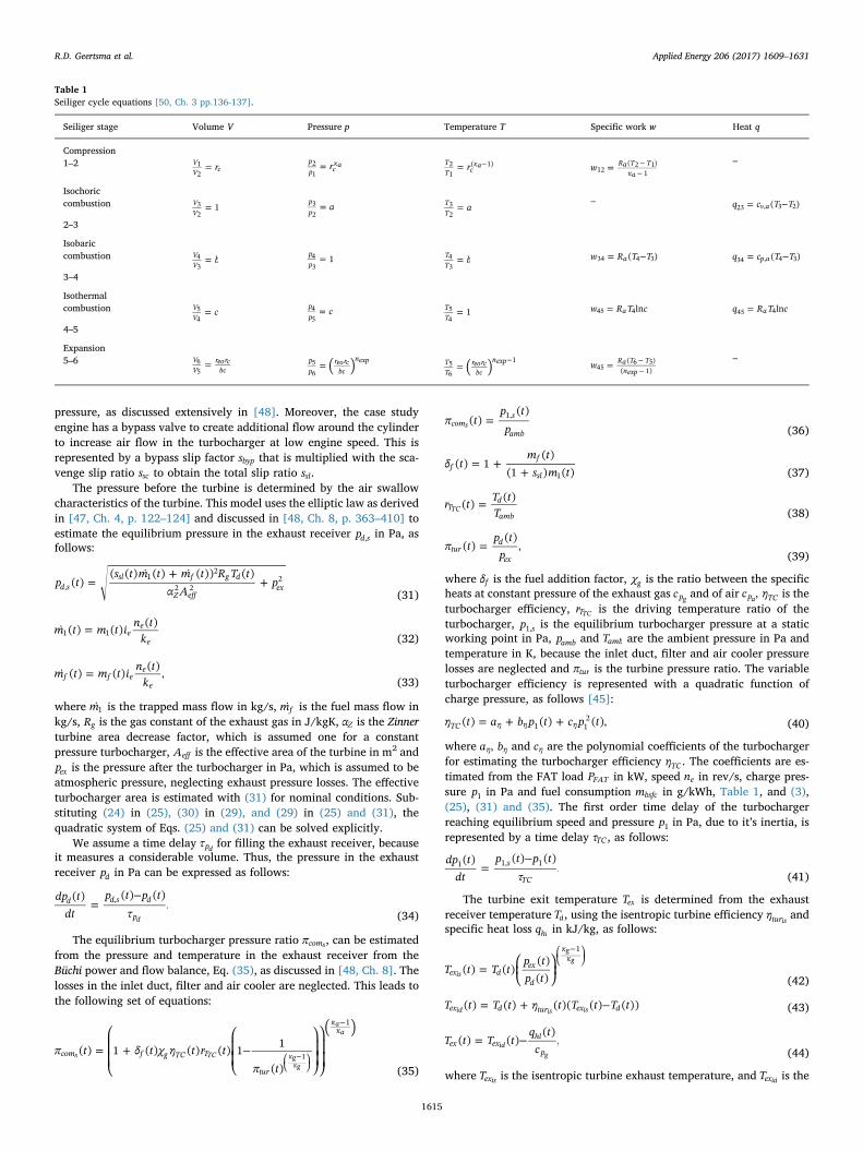
Waves can cause serious disturbances on the loading of diesel en-gines when a ship sails in high sea states, particularly when the engineruns in speed control. [8] has documented measurements on a KarelDoorman class frigate sailing in head waves in Sea State 6, which is theworst case scenario within normal operations according to typical de-sign specifications. These measurements, shown in Fig. 6, clearly il-lustrate how the disturbance of waves can cause engine overloading.

The main cause of the disturbance on engine loading is the fluctu-ating wake speed of the water flowing into the propeller, as previouslydiscussed in [10]. The orbital movement of water causes a disturbanceon the average speed of the water entering the propeller, an exponentialdistribution of water speed along the depth of the propeller and an


1617

oblique inflow. In this study, we are interested in the significant dis-turbance of the wave orbital movement on the propeller loading, due tothe significant wave height [72,73]. We therefore consider the wavespeed at the propeller centre, as follows:

= − −v t ζωe sin kv ω t( ) (( ) )wk z

sw (72)

=k ωg

,w2

(73)

where ζ is the significant wave amplitude in m, ω is the wave radialfrequency in rad/s, kw is the wave number in 1/m, z is the water depthin m at the propeller centre and g is the standard gravity in m/s2.

In summary, the ship propulsion system model consists of 4 sub-models with a system of Differential and Algebraic Equations (DAEs)and the wave sub-model with an Algebraic Equation (AE), with therelations shown in Fig. 2. The model consists of 6 state variables: fuelinjection per cylinder per cycle mf , charge pressure p1, exhaust receiverpressure pd, propeller speed np, propeller pitch Pp and ship speed vs. Theoverall system is thus composed of the diesel engine DAEs (1), (4), (5),(13)–(18), Table 1, (21)–(25) and (29)–(55), the gearbox DAEs (56) and(58)–(60), the propeller DAEs (62)–(68), the hull DAE (71) and thewave AE (72).

3. Conventional control

3.1. Control objectives

The objective for the conventional control strategy is to representthe control system implemented on the case study, the Holland classpatrol vessel. The control objectives for this baseline control strategy,used to validate the propulsion system model, are:

• Provide requested virtual shaft speed nvirt as defined in [7]:

=−−

n tP t PP P

n( )( )

,virtp p

p pp

nom

0

0 (74)

where Pp0 is the pitch ratio at which zero thrust is achieved and Ppnomis the nominal pitch ratio.

• Prevent engine overloading in design conditions by limiting thetelegraph position acceleration rate, limiting the pitch increase rateas a function of virtual shaft speed and reducing pitch when theengine margin is too small.

• Provide high manoeuvrability within engine overloading limitations

in manoeuvring mode for design conditions.

• Provide high propulsion efficiency within engine overloading lim-itations in transit mode for design conditions.

3.2. Control system design

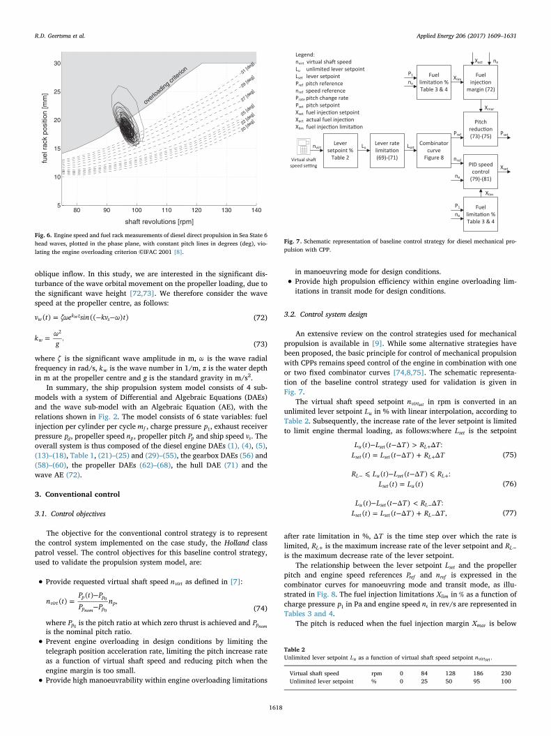
An extensive review on the control strategies used for mechanicalpropulsion is available in [9]. While some alternative strategies havebeen proposed, the basic principle for control of mechanical propulsionwith CPPs remains speed control of the engine in combination with oneor two fixed combinator curves [74,8,75]. The schematic representa-tion of the baseline control strategy used for validation is given inFig. 7.

The virtual shaft speed setpoint nvirtset in rpm is converted in anunlimited lever setpoint Lu in % with linear interpolation, according toTable 2. Subsequently, the increase rate of the lever setpoint is limitedto limit engine thermal loading, as follows:where Lset is the setpoint

after rate limitation in %, TΔ is the time step over which the rate islimited, +RL is the maximum increase rate of the lever setpoint and −RL

is the maximum decrease rate of the lever setpoint.The relationship between the lever setpoint Lset and the propeller

pitch and engine speed references Pref and nref is expressed in thecombinator curves for manoeuvring mode and transit mode, as illu-strated in Fig. 8. The fuel injection limitations Xlim in % as a function ofcharge pressure p1 in Pa and engine speed ne in rev/s are represented inTables 3 and 4.

The pitch is reduced when the fuel injection margin Xmar is below

80 90 100 110 120 130 1405

10

15

20

25

30

shaft revolutions [rpm]

fuel

rac

k po

sitio

n [m

m]

overlo

ading crite

rion

31 [deg]

29 [deg]

27 [deg]

eg]25 [deg]

20 [22 [d

deg]

Fig. 6. Engine speed and fuel rack measurements of diesel direct propulsion in Sea State 6head waves, plotted in the phase plane, with constant pitch lines in degrees (deg), vio-lating the engine overloading criterion ©IFAC 2001 [8].

neXact

Lu

Xset

Xlim

ne

Pset

Xlimne

P1

nref

Pref

Lsetnvirt

Virtual shaspeed se ng

Legend:nvirt virtual sha speedLu unlimited lever setpointLset lever setpointPref pitch referencenref speed referencePrate pitch change ratePset pitch setpointXset fuel injec on setpointXact actual fuel injec onXlim fuel injec on limita on

Lever setpoint %

Table 2

Combinator curve

Figure 8

Fuel limita on % Table 3 & 4

Fuel injec on

margin (72)

Xmar

Pitch reduc on(73)-(75)

PID speed control

(79)-(81)

ne

P1 Fuel limita on % Table 3 & 4

Lever rate limita on (69)-(71)

Fig. 7. Schematic representation of baseline control strategy for diesel mechanical pro-pulsion with CPP.

Table 2Unlimited lever setpoint Lu as a function of virtual shaft speed setpoint nvirtset .

Virtual shaft speed rpm 0 84 128 186 230Unlimited lever setpoint % 0 25 50 95 100

− − >= − +

+

+

L t L t T R TL t L t T R T

( ) ( Δ ) Δ :( ) ( Δ ) Δ

u set L

set set L (75)

⩽ − − ⩽=

− +R L t L t T RL t L t( ) ( Δ ) :

( ) ( )L u set L

set u (76)

− − <= − +

−

−

L t L t T R TL t L t T R T

( ) ( Δ ) Δ :( ) ( Δ ) Δ ,

u set L

set set L (77)


1618

Xmarmin in order to prevent thermal overloading and the pitch increaserate +RP is limited according to the linear relationship f1 shown inTable 5, as follows:

= −X X Xmar lim set (78)

< =+X X R R:mar mar P Prmin (79)

⩾ =+X X R f n: ( )mar mar P virt1min (80)

where Xset is the fuel injection setpoint for the fuel pump in % and nvirtis the actual virtual shaft speed in rpm.

Subsequently, the pitch setpoint Pset is represented by the followingequations:

where −RP is the maximum decrease rate of the pitch setpoint.The controller algorithm for the engine speed control that provides

the fuel injection setpoint Xset is as follows:

∫⎜ ⎟ ⎜ ⎟= ⎛⎝

− ⎞⎠

+ ⎛⎝

− ⎞⎠

X t Kn t n t

nK

n t n tn

dt( )( )

100( ) ( )

100( )

PID Pref e

eI

t ref e

e0nom nom (84)

⩽ =X t X t X t X t( ) ( ): ( ) ( )PID lim set PID (85)

> =X t X t X t X t( ) ( ): ( ) ( ),PID lim set lim (86)

where XPID is the unlimited fuel injection setpoint, KP is the proportionalgain and KI is the reset rate. The control parameters are listed in Table 6.

3.3. Control system tuning

The settings of the control parameters in Tables 2–6 and Fig. 8 havebeen determined through extensive dynamic simulations [71]. Becausethe relationship between the control parameters and the propulsionsystem MOEs is not very clear and depends on the operational condi-tions, the tuning requires weeks of analysing simulation time traces.Moreover, while the risk of thermal overloading has been eliminated,manoeuvrability, cavitation noise and fuel consumption might sufferfrom the conservative settings. However, the lack of MOPs to quantifysystem performance, has limited a thorough analysis of the trade-offbetween the various MOEs.

4. Validation of propulsion system model with conventionalcontrol

We use the terminology for model qualification, verification andvalidation as proposed in [76]. The model qualification, the analysis toobtain the conceptual model, and the conceptual model itself have beendescribed in Section 2. We have performed the model verification persubsystem, as proposed in [17], for each of the subsystem models byvarying the input parameters and comparing the response with analy-tical results (see Fig. 12 and 15).

Validation procedures with statistical analysis for a complex mul-tidisciplinary simulation model have been described in [77–79,17,80].[78] quantifies the uncertainty of the static model results by estimatingthe parameter uncertainty and running the simulation model for theextremes of the 95% confidence interval for the full model. Alter-natively, [77] proposes to estimate the parameter uncertainty andsubsequently determine the sensitivity of the sub-model either mathe-matically with Taylor approximations or numerically with in-finitesimally small disturbances. Subsequently, the total ship modeluncertainty can be established with linearisation by first order Taylorapproximations. [79] compares these two methods with a case studyand concludes the method proposed in [77] is more efficient whiledelivering comparable results. Subsequently, the validity of the modelcan be determined by comparing the model result interval with theconfidence interval of measurements [78]. Another widely usedmethod, Monte Carlo simulation, has been applied to a propulsionsystem model in [80]. While this method can handle non-linearities, asopposed to the method in [77], it does not provide insight in systembehaviour. The main drawback of all these approaches is that theoutcome of the statistical analysis strongly depends on the estimatedparameter uncertainty and that other types of uncertainty are not ad-dressed.

In our case, we want to establish how well we can predict the be-haviour of a propulsion plant in uncertain operational conditions basedon the model and its calibration with Factory Acceptance Test (FAT)data and determine how we can use this model to quantify the per-formance of the system and its control strategy for various MOEs.Subsequently, we want to use it to analyse the influence of the controlstrategy on the performance of the system as a whole quantifiedthrough a number of MOPs. Therefore, in this study we carry outquantitive validation with measurements of the ship in real operationalconditions during the ships SAT.

telegraph position setpoint [%]0 10 20 30 40 50 60 70 80 90 100

shaf

t spe

ed [%

] and

rela

tive

pitc

h se

tpoi

nt [%

]

0

10

20

30

40

50

60

70

80

90

100Combinator curves

shaft speed for manoeuvring mode combinatorrelative pitch setpoint for manoeivring mode combinatorshaft speed for transit mode combinatorrelative pitch setpoint for transit mode combinator

Fig. 8. Combinator curves for baseline control strategy in manoeuvring and transitmodes.

Table 3Fuel injection limitation Xlim as a function of charge pressure p1.

Absolute charge pressure kPa 0 100 300 350 400 500Fuel injection limitation % 42 42 103 109 115 115

Table 4Fuel injection limitation Xlim as a function of engine speed ne.

Engine speed rpm 400 500 500 700 800 900 1000Fuel limitation % 40 46 55 67 84 105 105

Table 5Pitch increase rate +RP as a linear interpolation function f1 of virtual shaft speed nvirt .

Virtual shaft speed rpm 0 40 77 153 190 230 240Pitch increase rate %/s 3 2 1 1 0.5 0.2 0.2

− − >= − +

+

+

P t P t T R TP t P t T R T

( ) ( Δ ) Δ :( ) ( Δ ) Δ

ref set P

set set P (81)

⩽ − − ⩽=

− +R P t P t T RP t P t

( ) ( Δ ) :( ) ( )

P ref set P

set ref (82)

− − <= − +

−

−

P t P t T R TP t P t T R T

( ) ( Δ ) Δ :( ) ( Δ ) Δ ,

ref set P

set set P (83)


1619

4.1. Diesel engine model validation

The diesel engine models proposed in this study, or earlier versionsproposed in [24,10], have not been validated in previous work.Therefore, this section first discusses the parametrisation and calibra-tion of the model, based on the approach described in [17]. Subse-quently, a quantitative validation wil be discussed using the full FATdata.

The parameters used in the diesel engine model have been obtainedfrom four sources. Most engine parameters are available from the en-gine project guide and operating manual [81,12]. Furthermore, someparameters have been estimated based on diesel engine theory [50,48]or general physics theory. Finally, FAT results have given the remainingparameters, for calibration of the turbocharger efficiency as a functionof the charge pressure, heat loss as a function of air flow and turbo-charger entry temperature and heat release as a function of enginespeed. The diesel engine parameters and their source have been sum-marised in Table 7.

The model is run at the FAT speed and power settings with theparameters from Table 7. The results in Figs. 9–11 show that the FATmeasurements for specific fuel consumption, charge air pressure,combustion pressure, fuel injection and exhaust receiver temperatureare within 5% of the model predictions. The turbocharger exit tem-perature is also reasonably predicted with the model, although thedeviation at 25% load is slightly higher at 8%.

The FAT measurement data only consists of a limited amount ofoperating points in the full engine operating envelope, along the pro-peller curve. Full validation of the model requires measurements acrossall operating points of the engine. Therefore, a more extensive mea-surement campaign is recommended for further model validation. Forcompleteness, Fig. 12 shows the specific fuel consumption and the airexcess ratio over the complete operating envelope of the engine. Whencomparing this with the specific fuel consumption of a typical highspeed engine in Fig. 14, as published in [11], the model results arewithin 5% down to 10% load of the engine. The minimum air excessratio within the engine operating envelope is 1.4. This value can serveas a minimum air excess ratio that needs to be maintained in dynamicconditions. Fig. 13 shows the exhaust valve temperature and the ex-haust receiver temperature, and therefore the entry temperature of theturbine. The trend of the exhaust valve temperature exactly matches thetrend of the air access ratio, as previously demonstrated with modellingand experiments in [43]. This confirms that the air access ratio canserve as a good indicator for engine thermal loading. Although thetrend of the exhaust receiver temperature shows an even bigger dis-continuity at 900 rpm, the speed below which the cylinder bypass valveopens and provides extra cooling air to the exhaust receiver, the ex-haust receiver temperature is also strongly influenced by the air accessratio.

4.2. Gearbox model validation

The gearbox loss model parameters a b,gb gb and cgb and the nominalgearbox loss Plnom in W were obtained from a linear fit through threedata points of the gearbox manufacturer data and are presented in

Table 8. When inspecting the results from the gearbox loss model inFig. 15 and comparing them with the losses obtained from the manu-facturers data over the full torque and speed envelop, we establish thatthe obtained values are within 1%, confirming the visual impressionthat the gearbox power losses exhibit a quadratic relationship withengine speed.

4.3. Propeller model validation

Available propeller models and data series have been discussed in[10] and an extensive review is available in [82]. In this study we usethe Wageningen CD series, which represent ‘contemporary and prac-tical CPP designs’ [60]. Moreover, the 5 blade propellers in this seriesrepresent CPP design ‘aimed at applications for the navies’ [60] and thedesign compromise was focused on ‘better cavitation performance forhigh pitch and large blade area ratios ’ [60]. We use the WageningenC5-60 propeller, which has been made available to the partners in theJoint Industry Project on developing the Wageningen C- and D-seriesfor Controllable Pitch Propellers (CPPs). This propeller has a similaropen water diagram to the propeller fitted to the Holland class patrolvessel. The propeller parameters are presented in Table 9.

Because the Wageningen C5-60 propeller is not yet publicly avail-able, this paper does not present the model results of this propeller

Table 6Control parameters in manoeuvring mode (MAN) and transit mode (TRAN)

Propulsion mode MAN TRAN

Proportional gain KP 2 2Reset rate KI 0.5 0.5Maximum lever increase rate +RL 1.5%/s 3%/sMaximum lever decrease rate −RL −3%/s −6%/sPitch reduction rate RPr −1.89%/s −1.89%/sMinimum injection margin Xmarmin 16.5% 16.5%Maximum pitch reduction rate −RP −10%/s −10%/s

Table 7Patrol vessel case study diesel engine model parameters from project guide (PG), physicstheory (P), FAT data (F) or estimate (E).

Diesel engine parameter description Value Source

Nominal engine power Penom 5400 kW PGNominal engine speed nenom 16.71 rev/s PGNumber of cylinders ie 12 PGNumber of revolutions per cycle ke 2 PGBore diameter DB 0.28 m PGStroke length LS 0.33 m PGCrank rod length LCR 0.64063 PGCrank angle after TDC, inlet closure αIC 224 ° PGCrank angle after TDC, exhaust open αEO 119 ° PGNominal spec. fuel consumption mbsfcnom 198 g/kW h PGHeat release efficiency ηq 0.886 PG

Geometric compression ratio εc 13.8 PGTotal nominal mass flow mtnom 10.5 kg/s PGCylinder volume at state 1 V1 0.0199 m3 PGNominal pressure at state 1 p nom1 4.1e5 Pa PG

Maximum cylinder pressure pmaxnom 188e5 Pa PG

Temperature after the intercooler Tc 323 K PGTemperature of the inlet duct Tinl 423 K EParasitic heat exchanger effectiveness εinl 0.05 EFuel injection time delay τX 0.0151 s ETurbocharger time constant τTC 51 s EExhaust receiver time constant τpd 0.01 s EGas constant of air Ra 287 J/kg K PSpecific heat at constant volume of air cv a, 717.5 J/kg K PSpecific heat at const. pressure of air cp a, 1005 J/kg K PSpecific heat at const. p of exhaust gas cp g, 1100 J/kg K PIsentropic index of air κa 1.4 PIsentropic index of the exhaust gas κg 1.353 P

Lower heating value of fuel hL 42700 J/kg PGStoichiometric air to fuel ratio σf 14.5 PGPolytropic exponent for expansion nexp 1.38 EPolytropic exponent for blowdown nbld 1.38 ENominal mechanical efficiency ηmnom 0.90 E

Constant volume portion gradient Xcvgrad −0.4164 F

Constant temperature portion Xctnom 0.4 ETurbocharger factor aη −3.29e−12 FTurbocharger factor bη −2.52e−6 F

Turbocharger factor cη 0.2143 FAmbient pressure pamb 1e5 Pa PGAmbient temperature Tamb 318 K PG


1620

separately. Clearly, the model uses the results of the open water tests,which is a well accepted method to model propeller thrust and torquewithin the assumptions of a homogenous advance speed, perpendicularflow into the propeller and quasi static performance. However, themodelling strategy and software code needs to be verified. For ver-ification purposes we refer to the results of the C4-40 propeller pre-sented in [10], which can be compared with the results presented in[19]. Moreover, for an uncertainty analysis of the method used to de-termine the Wageningen C- and D-series propellers, we refer to [60].

4.4. Hull and wave model validation

The ship resistance and the wave model parameters very stronglydepend on the conditions in which the ship operates. In order to in-vestigate the effect of varying conditions we consider three typicalconditions. Trial condition is defined as Sea State 0, wind speed of 3 m/s and no fouling. Service condition is defined as Sea State 4, wind speedof 11 m/s, head seas and wind and 6 months out of dock fouling. Off-design condition is defined as Sea State 6, wind speed of 24 m/s, headseas and wind and 6 months out of dock fouling. The parameters thatrepresent these conditions are shown in Table 10 and Fig. 16.

600 650 700 750 800 850 900 950 1000 1050

engine speed [rpm]

180

190

200

210

220

230

brak

e sp

ecifi

c fu

el c

onsu

mpt

ion

[g\k

Wh]

Specific fuel consumption model validation

model results+5% error margin of model-5% error margin of modelFAT measurements

600 650 700 750 800 850 900 950 1000 1050

engine speed [rpm]

1

2

3

4

5

char

ge a

ir pr

essu

re [b

ar]

Charge air pressure model validation


Fig. 9. Diesel engine model validation with FAT results for specificfuel consumption and charge air pressure.

600 650 700 750 800 850 900 950 1000 1050

engine speed [rpm]

50

100

150

200

250

max

imum

com

bust

ion

pres

sure

[bar

]

Maximum combustion pressure model validation


600 650 700 750 800 850 900 950 1000 1050

engine speed [rpm]

1

1.5

2

2.5

3

3.5

4

exha

ust r

ecei

ver p

ress

ure

[bar

] Exhaust receiver pressure model validation


Fig. 10. Diesel engine model validation with FAT results for max-imum combustion pressure and exhaust receiver pressure.


1621

The validation of resistance test results is routinely performed byorganisations such as MARIN, who have performed the resistance test.However, the total ship model validation demonstrates that the model’sresulting ship speed corresponds with the tow tank test results. Theverification of the behaviour of the propulsion plant in waves is per-formed with the total ship model based on ship measurements.

4.5. Total ship model validation

The total ship model consists of all the models discussed in Section 2and of the control strategy described in Section 3.2. The parameters and

validation of these models have been discussed in the previous Sections.The aim of this Section is to quantitatively validate the dynamic behaviourof the total ship model including the conventional control strategy. To thisend, we compare the simulation results of an acceleration manoeuvre withthe actual measurements of the same acceleration manoeuvre performedduring the SAT’s of HNLMS Holland, shown in Fig. 17. Even though theavailable measurements are limited, the available measurements delivergood confidence in the model credibility. Moreover, we compare the be-haviour of the propulsion plant sailing at constant speed in waves withearlier measurements performed on a Karel Doorman class frigate in SeaState 6 as reported in [8].

600 650 700 750 800 850 900 950 1000 1050

engine speed [rpm]

300

400

500

600

700

800

Exha

ust g

as re

ceiv

er te

mpe

ratu

re [K

]

Exhaust gas receiver temperature model validation


600 650 700 750 800 850 900 950 1000 1050

engine speed [rpm]

200

300

400

500

600

700

Turb

ocha

rger

exi

t tem

pera

ture

[K] Turbocharger exit temperature model validation


Fig. 11. Diesel engine model validation with FAT results for exhaustreceiver and turbocharger exit temperature.

400 600 800 1000

speed [rpm]

0

500

1000

1500

2000

2500

3000

3500

4000

4500

5000

pow

er [k

W]

Brake specific fuel consumption contour [g/kWh]

197

198

199

200

205

210

220

240260

260

300300

400 400600 600

power limit [kW]bsfc [g/kWh]

400 600 800 1000

speed [rpm]

0

500

1000

1500

2000

2500

3000

3500

4000

4500

5000

pow

er [k

W]

Air excess ratio contour

1.4

1.6

1.6

1.8

1.8

1.8

1.8

2

2

2

2.2

2.2

2.6

2.6

33

4 45

power limit [kW]air excess ratio [-]

Fig. 12. Diesel engine model specific fuel consumption and air excessratio results in complete operating envelope of the engine.


1622

4.5.1. Acceleration manoeuvreThe results of the acceleration manoeuvre from zero ship speed and a

virtual shaft speed of 0 rpm to a setpoint of 230 rpm virtual shaft speed attime =t 30 s are presented in Figs. 18–20. The model results during themanoeuvre for fuel injection, shaft speed and virtual shaft speed staywithin 5% of the measurements. The pitch has a larger deviation, but thisis caused by the different open water diagram of the actual propellercompared to the C5-60 propeller that was used in the model.

The following main differences between the model results and themeasurements can be identified:

• The model fuel pump position is approximately 2.5% higher thanthe measured fuel pump position at the start of the manoeuvre whenthe diesel engine load is below 10%. The results in Fig. 12 and 14show the overestimated fuel consumption of the model causes thisdifference. This can possibly be resolved with more accurate mod-elling of the heat losses during expansion and blowdown after per-forming a more extensive measurement campaign on an engine, asdiscussed in Section 4.1.

• The response of the actual pitch has a time variant dead time ofmaximum 2 s on top of the linear delay. This delay is mainly causedby the counter balance valve as described in detail in [63]. [63]proposes to either remove the counter balance valve or maintain thecontrol pressure of the counter balance valve if a fast pitch actuationis required to support an angle of attack control strategy as proposedin [7]. Then, a pitch actuation bandwidth of 0.6 Hz can be achieved.Alternatively, the nonlinear effects could be included in the modelas proposed in [63,65,66] or the nonlinear effects could be ne-glected and the pitch actuation bandwidth of the model could bereduced to 0.15 Hz, leading to =τ 6.7P .

• The actual engine margin between =t 105 s and =t 130 s is sig-nificantly higher than the predicted engine margin. Because thecharge pressure has not been logged the actual cause of this differ-ence cannot be accurately determined. A possible cause is the non-linear behaviour of the pitch actuation. However, the propeller pitchand engine loading of the model and the measurements in this timebracket do behave similarly. Therefore, the predicted performanceof the total system model stays within 5% of the actual

400 600 800 1000

speed [rpm]

0

500

1000

1500

2000

2500

3000

3500

4000

4500

5000

pow

er [k

W]

Exhaust valve temperature contour [bar]

650700 800800

900900

10001050

1050

1100

1100

1100

1175

1175

1175

1300

power limit [kW]exhaust valve temperature [K]

400 600 800 1000

speed [rpm]

0

500

1000

1500

2000

2500

3000

3500

4000

4500

5000

pow

er [k

W]

Outlet receiver temperature contour [bar]

600 650650700

700750

750

750

800800

800

800

850

850

850

850

850

power limit [kW]outlet receiver temperature [K]

Fig. 13. Diesel engine model exhaust valve and exhaust receivertemperature results in complete operating envelope of the engine.

Fig. 14. Specific fuel consumption of typical high speed engine from [11].

Table 8Gearbox parameters.

Gearbox loss parameter agb 0

Gearbox loss parameter bgb 0.75

Gearbox loss parameter cgb 0.25Gearbox nominal power loss Plnom in kW 109Gearbox speed reduction ratio igb 4.355Nominal propeller speed n pnom in rpm 230Total inertia Jt in kg m2 4600


1623

measurements.

• The combinator setpoint signal measured during the SAT exhibitswhat appears to be a high amount of signal noise. The signal issupposed to be constant at 93.5%, which is the final pitch setpointassociated with the virtual shaft speed of 230 rpm. Moreover, thesignal features a spike at t = 30 s, before following the expectedramp. The cause of this noise is unknown but does not appear toinfluence the overall system response.

In summary, this quantitative validation demonstrates that themodel predicts the total propulsion system behaviour within 5%.

4.5.2. Sailing in heavy seasMeasurements of sailing in heavy seas of the patrol vessel are not

available. The only available measurements of a similar ship sailing inheavy seas have been reported in [17,8]. [8] report the measurements

of a Karel Doorman class frigate in Sea State 6 and the results of thesemeasurements are shown in Fig. 6.

To use these measurements for verification of the modellingstrategy, we have changed the model parameters to reflect the mainparameters of a typical frigate. The parameters used are shown inTable 11. For the hull and wave model parameters off-design conditionsare assumed, as the reported results have been obtained in Sea State 6.Moreover, the pitch reduction strategy was not used in this simulation,because during the measurements no pitch reduction strategy was in-cluded in the control strategy and overloading actually occurred.Fig. 21 shows the results at 100 rpm virtual shaft speed of the propul-sion system model that is modified to reflect a Karel Doorman classfrigate.

The results in Fig. 21 demonstrate that the average magnitude of thedisturbance of the engine speed and fuel injection due to the waves ispredicted well: the fuel rack position fluctuates between 15 and 22 mm,with a nominal fuel rack position of 30 mm. The irregular effects ofwaves that clearly appear in the measurements in Fig. 6, are neglectedin the model. Therefore, the propulsion system model does not predictthe extreme values of the disturbance due to waves, but predicts theeffect due to the significant wave height [73].

An accurate statistical analysis of the uncertainty of the modelcannot be performed with these measurements, because the sea stateonly roughly determines the range of the wave height. For example, SeaState 6 is defined as a significant wave height between 4 and 6 m. Moreaccurate loggings or measurements of the actual wave height would berequired as input data for an accurate statistical analysis.

5. Measures of performance

Various standardised operating profiles have been determined in theautomotive field to evaluate and compare MOPs of energy managementstrategies for hybrid electric vehicles, such as the world-harmonisedlight-duty vehicle test cycle (WLTC) and the new European drivingcycle (NEDC) [83]. Moreover, a control benchmark simulation modelexists for these control strategies [84]. These standards have not yetbeen defined for the evaluation of ship control strategies. Altosole et al.[85,86] propose the slam start and crash stop manoeuvres to evaluatecontrol strategy performance during the most extreme acceleration anddeceleration manoeuvres. While these manoeuvres are very valid to

Gearbox output shaft speed [rpm]0 100 200 300 400 500 600 700 800 900 1000 1100

Gea

rbox

die

sel e

ngin

e in

put p

ower

[kW

]

0

1000

2000

3000

4000

5000

6000

1020

20

30

30

40

40

50

50

50

60

60

60

70

70

70

80

80

80

90

90100

Gearbox loss contour plot for diesel engine mode

Base pointsPropeller curveGearbox loss [kW]

Fig. 15. Gearbox loss model contour plot with the three data pointsused for the linear fit and the propeller curve.

Table 9Propeller parameters.

Wake fraction w 0.08Relative rotative efficiency ηR 1Propeller diameter D in m 3.2Design pitch ratio at 0.7R Pd 0.8Nominal pitch ratio at 0.7R Pnom 1.18Pitch ratio for zero thrust P0 0.068First order pitch actuation delay τP 1.67Vrijdag coefficient c1 0.7Shock free entry angle αi 0

Table 10Hull and wave model parameters in trial, design and off-design condition.

Condition Trial Service Off-design

Ship mass m in 103kg 3800Number of propellers m 2Thrust deduction factor t 0.155Propeller centre depth z in m 6.5Wave amplitude ζ in m 0 1 2.5Wave frequency ω in rad/s – 0.966 0.628Wave number k – 0.095 0.0402


1624

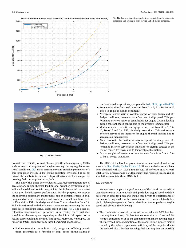
evaluate the feasibility of control strategies, they do not quantify MOEs,such as fuel consumption and engine loading, during regular opera-tional conditions. [87] maps performance and emission parameters of aship propulsion system in the engine operating envelope, but do notextend the analysis to measure ships effectiveness, for example ex-pressing fuel consumption in ton/mile.

The aim of this paper is to evaluate MOEs fuel consumption, rate ofacceleration, engine thermal loading and propeller cavitation with avalidated model and obtain insight into the influence of the controlstrategy on holistic system performance. For this purpose, we proposethe following benchmark manoeuvres: sail at constant speed in trial,design and off-design conditions and accelerate from 0 to 5, 5 to 10, 10to 15 and 0 to 15 kts in design conditions. The acceleration from 0 to15 kts is performed with the slam start manoeuvre: increasing the leversetpoint to maximum virtual shaft speed at once [65]. The other ac-celeration manoeuvres are performed by increasing the virtual shaftspeed from the setting corresponding to the initial ship speed to thesetting corresponding to the final ship speed. Moreover, we propose thefollowing MOPs, obtained from these benchmark manoeuvres:

• Fuel consumption per mile for trial, design and off-design condi-tions, presented as a function of ships speed during sailing at

constant speed, as previously proposed in [61, Ch12, pp. 482–483];

• Acceleration time for speed increases from 0 to 5, 5 to 10, 10 to 15and 0 to 15 kts in design conditions;

• Average air excess ratio at constant speed for trial, design and off-design conditions, presented as a function of ship speed. This per-formance criterion serves as an indicator for engine thermal loadingduring constant speed sailing due to the average temperature;

• Minimum air excess ratio during speed increases from 0 to 5, 5 to10, 10 to 15 and 0 to 15 kts in design conditions. This performancecriterion serves as an indicator for engine thermal loading due toacceleration manoeuvres;

• Air excess ratio fluctuation at constant speed for design and off-design conditions, presented as a function of ship speed. This per-formance criterion serves as an indicator for thermal stresses in theengine caused by waves due to temperature fluctuation;

• Cavitation plot of acceleration manoeuvres from 0 to 5 and 5 to10 kts in design conditions.

The MOPs of the baseline propulsion model and control system areshown in Figs. 22–26, Tables 12 and 13. These simulation results havebeen obtained with MATLAB Simulink R2016b software on a PC withIntel Core i7 processor and 16 GB memory. The required time to run allsimulations to obtain these MOPs is 1 h.

5.1. Discussion

We can now compare the performance of the transit mode, with acombinator curve with relatively high pitch, low engine speed and slowacceleration rates for pitch and engine speed, with the performance ofthe manoeuvring mode, with a combinator curve with relatively lowpitch, high engine speed and fast acceleration rates for pitch and enginespeed and observe the following:

• The combinator curve of the transit mode achieves 30% less fuelconsumption at 5 kts, 10% less fuel consumption at 10 kts and 2%less fuel consumption at 15 kts compared to the manoeuvring mode.The increased fuel consumption of the manoeuvring mode is mainlycaused by the reduced open water efficiency of the propeller due tothe reduced pitch. Further reducing fuel consumption can possibly

ship speed [kts]0 5 10 15 20 25

ship

resi

stan

ce [k

N]

0

200

400

600

800

1000

1200

1400resistance from model tests corrected for envronmental conditions and fouling

trial conditionservice conditionoff-design condition

Fig. 16. Ship resistance from model tests corrected for environmentalconditions and fouling in trial, service and off-design condition.

Fig. 17. Zr. Ms. Holland.


1625

be achieved by further increasing the pitch during transit modewhen the engine loading allows this, in trail and design conditions.In off-design conditions, however, the difference in fuel consump-tion disappears, because the pitch reduction enforces the same re-duced pitch for the transit mode to prevent overloading of the en-gine.

• The air excess ratio at constant speed in manoeuvring mode is0.1–0.3 higher than in transit mode, at low speeds when the pitchreduction mechanism is not limiting pitch. This lower air excessratio leads to a significantly lower thermal loading of the engine, ofapproximately 30–90 K. This is caused by the lower pitch and higherengine revolutions and enables using higher acceleration rates forpitch and engine speed without thermally overloading the engine.

Due to these high acceleration rates the acceleration time of the shipis in average 2 times faster in manoeuvring mode than in transitmode.

• In order to investigate the methodology of using the cavitation plotto assess the cavitation performance, we define a fictive cavitationbucket that matches the propeller and is centred at an angle of at-tack of 8 degrees. However, the shown cavitation buckets for thesepropeller have not been determined through measurement and areonly shown to give some indication of the control strategy influenceon cavitation behaviour. With this fictive cavitation bucket, thecombinator curve of the transit mode falls within this bucket up to aspeed of 10 kts for static conditions and only slightly violates thecavitation bucket during acceleration manoeuvres up tot the same

0 50 100 150 200 250time [s]

0

50

100

150

200

250

shaf

t spe

ed a

nd v

irtua

l sha

ft sp

eed

spee

d [rp

m]

shaft speed and virtual shaft speed from model and measurements

model shaft speedmodel virtual shaft speedSAT actual shaft speedSAT virtual shaft speed

Fig. 18. Total ship model validation with SAT results for shaft speedand virtual shaft speed.

0 50 100 150 200 250time [s]

-10

0

10

20

30

40

50

60

70

80

90

100

prop

elle

r pitc

h [%

]

propeller pitch time trace

combinator setpointactual pitchSAT combinator setpointSAT actual pitch

Fig. 19. Total ship model validation with SAT results for engineloading and margin.


1626

speed. Alternatively, the low pitch of the manoeuvring mode causesit to significantly violate the cavitation bucket. The cavitation plotsfor constant speed sailing and acceleration manoeuvres are bothpositioned outside the typical cavitation bucket.

In conclusion, the MOPs can be used to quickly and quantitativelyasses the performance of a control strategy and its parameters.Moreover, these benchmark manoeuvres and performance criteria canbe used to compare performance of alternative control strategies, butalso of alternative propulsion configurations.

6. Conclusions and future research

A method is required to objectively and quickly quantify and assessthe effectiveness of the system architecture and control strategy fordiesel mechanical and hybrid propulsion systems. We have proposed anew diesel propulsion system model that can be parameterised withavailable manufacturer data. This model is based on a previous MeanValue First Principle (MVFP) model and has been improved to reflect

0 50 100 150 200 250time [s]

0

20

40

60

80

100

120

engi

ne li

mita

tion,

mar

gin

and

fuel

pum

p po

sitio

n [%

]

engine loading and limitation

model charge air limitationmodel fuel pump positionmodel engine marginactual fuel pump positionactual engine margin

Fig. 20. Total ship model validation with SAT results for propellorpitch and propeller pitch setpoints.

Table 11Changed propulsion model parameters to simulate a typical frigate, si-milar to Karel Doorman class at 100 rpm virtual shaft speed.

Parameter value

Propeller diameter in m 4.2Propeller pitch ratio at 100 rpm 1.2Gearbox ratio 7.3

shaft speed [rpm]50 60 70 80 90 100 110 120 130 140

fuel

rack

pos

ition

[mm

]

5

10

15

20

25

30

35

engine envelopetemporary operation limitPredicted engine behaviour in off-design conditions for frigate

Fig. 21. Total ship model validation of simulated M-frigate at 100 rpmin Sea State 6.


1627

modern turbocharger and Miller-timing behaviour based on advanceddiesel engine theory. Subsequently, we have validated the MVFP dieselengine model with measurements in factory conditions and in opera-tional conditions at sea with a case study naval vessel. The predictionsof the diesel engine model were within 5% of most measurement va-lues. Although exhaust gas temperatures were only predicted within10% of the measurements, the engine thermal loading can be accuratelyquantified with the air excess ratio.

The baseline control strategy with fixed combinator curves, accel-eration limitations and pitch reduction strategy has been described. We

have shown that this strategy can prevent engine overloading effec-tively while achieving conservative manoeuvrability, acceleration andcavitation behaviour. Quantitative validation has demonstrated that thepropulsion system model credibly predicts propulsion system behaviourwithin 5% accuracy. Moreover, the wave model behaviour in Sea State6 has been verified with the propulsion system model with modifiedparameters that reflect a frigate. The results of this model were found tomatch measurements on a frigate in Sea State 6.

Finally, the paper proposes benchmark manoeuvres and associatedmeasures of performance (MOPs) to quantify the performance of the

0 5 10 15 20 25ship speed [kts]

0

10

20

30

40

50

60

70

80

90

100

fuel

con

sum

ptio

n [k

g/m

ile]

Fuel consumption as a function of ship speedtrial conditions in manoeuvring modetrial conditions in transit modedesign conditions in manoeuvring modedesign conditions in transit modeoff-design-conditions in manoeuvring modeoff-design conditions in transit mode

Fig. 22. Fuel consumption plot as a function of ships speed for variousconditions in manoeuvring and transit mode.

0 5 10 15 20 25ship speed [kts]

1.5

2

2.5

3

3.5

4

4.5

air e

xces

s ra

tio

Air access ratio as a function of ship speed

trial conditions in manoeuvring modetrial conditions in transit modedesign conditions in manoeuvring modedesign conditions in transit modeoff-design-conditions in manoeuvring modeoff-design conditions in transit modeminimum air excess ratio

Fig. 23. Air excess ratio plot as a function of ships speed for variouscondition in manoeuvring and transit mode.


1628

propulsion plant on the following measures of effectiveness (MOEs):fuel consumption, rate of acceleration, engine thermal loading andpropeller cavitation. These MOPs and the propulsion system modelhave been used to evaluate the performance of two operating modes ofthe conventional control strategy. Analysing these two control modespreviously either required days of sea trials, or weeks of analysingvarious simulation time traces. Alternatively, the proposed MOPs canbe determined within an hour of simulation time. Depending on theparticular control strategy and operating conditions, fuel savings up to

30%, thermal loading reduction of 90 K and reductions of 50% in ac-celeration time can be achieved.

Future work will use the model proposed in this paper to evaluatean adaptive pitch control strategy that aims to reduce fuel consumptionand emissions, improve the ships manoeuvrability and reduce cavita-tion noise while preventing engine overloading. Adding an inductionmotor model, as proposed in [88] will allow to evaluate the perfor-mance of hybrid propulsion plants with CPP as well.

0 2 4 6 8 10 12 14 16 18 20

ship speed [kts]

0

0.1

0.2

0.3

0.4

0.5

0.6

air e

xces

s ra

tio fl

uctu

atio

n

Air access ratio fluctuation at constant speed due to wave disturbance

design conditions in manoeuvring modedesign conditions in transit modeoff-design-conditions in manoeuvring modeoff-design conditions in transit mode

Fig. 24. Air excess ratio fluctuation plot as a function of ships speedfor design and off-design conditions in manoeuvring and transit mode.

-2 0 2 4 6 8 10 12 14effective angle of attack

0

1

2

3

4

5

6

7

8

9

10

cavi

tatio

n nu

mbe

r

Cavitation plot

trial conditions in manoeuvring modetrial conditions in transit modedesign conditions in manoeuvring modedesign conditions in transit modefictive cavitation bucket

Fig. 25. Cavitation plot from low speed to maximum speed for variousconditions in manoeuvring and transit mode.


1629

Acknowledgement

This project is partially supported by project ‘ShipDrive: A NovelMethodology for Integrated Modelling, Control, and Optimization ofHybrid Ship Systems’ (project 13276) of Dutch Technology FoundationSTW and by the Royal Netherlands Navy. The Royal Netherlands Navysupplied Fig. 17. Fig. 6, ©IFAC 2001, was reproduced from [8] withpermission.

Special thanks goes to Maarten de Boer and Ilham Hardy ofShipdrive Partner Damen Schelde Naval Shipbuilding for preparing andproviding the validation data in FAT and SAT measurements and to dr.Arthur Vrijdag and prof. Douwe Stapersma for reviewing the manu-script and providing advice to improve the scientific quality andreadability of this article.

Appendix A. Supplementary material

Supplementary data associated with this article can be found, in theonline version, at http://dx.doi.org/10.1016/j.apenergy.2017.09.103.

References

[1] IMO. Third IMO greenhouse gas study 2014, exec. summary and final report. Tech.rep., IMO, London, UK; 2015.

[2] Roskilly AP, Palacin R, Yan J. Novel technologies and strategies for clean transport sys-tems. Appl Energy 2015;157:563–6. http://dx.doi.org/10.1016/j.apenergy.2015.09.051.

[3] van Oers B. A packing approach for the early stage design of service vessels [Ph.D.thesis]. The Netherlands: Faculty 3ME, Delft U of T; 2011.

[4] Roedler GJ, Jones C. Technical measurement, a coll. project of PSM, INCOSE andindustry. v 1.0 INCOSE-TP-2003-020-01. INCOSE; 2005.

[5] Grimmelius HT, Stapersma D. Control optimisation and load prediction for marinediesel engines using a mean value first principle model. In: Proc MS & TES,Newcastle-upon-Tyne, UK; 2000. p. 212–9.

[6] Grimmelius HT, Stapersma D. The impact of propulsion plant control on dieselengine thermal loading. In: Proc 22nd CIMAC WC, Hamburg, Germany; 2001.

[7] Vrijdag A, Stapersma D, van Terwisga T. Control of propeller cavitation in opera-tional conditions. J Mar Eng Technol 2010;16:15–26.

[8] Van Spronsen P, Toussain R. An optimal control approach to preventing marinediesel engine overloading aboard Karel Doorman class frigates. In: Proc. IFACCAMS, Glasgow, UK; 2001. p. 23–30.

[9] Geertsma RD, Negenborn RR, Visser K, Hopman JJ. Design and control of hybridpower and propulsion systems for smart ships: a review of developments. ApplEnergy 2017;194:30–54. http://dx.doi.org/10.1016/j.apenergy.2017.02.060.

[10] Geertsma RD, Negenborn RR. Visser K, Hopman JJ. Torque control for diesel me-chanical and hybrid propulsion for naval vessels. In: Proc. 13th INEC, Bristol, UK;2016. p. 476–92.

[11] van Straaten OFA, de Boer MJ. Optimum propulsion engine configuration from fueleconomic point of view. In: Proc 11th INEC, Edinburgh, UK; 2012.

[12] MAN Diesel SE. Project guide for marine plants diesel engine 28/33d prelim. Tech.rep. MAN Diesel SE, Augsburg, Germany; May 2008.

[13] Guan C, Theotokatos G, Zhou P, Chen H. Computational investigation of largecontainership propulsion engine operation at slow steaming conditions. ApplEnergy 2014;130:370–83. http://dx.doi.org/10.1016/j.apenergy.2014.05.063.

[14] Kyrtatos NP, Koumbarelis I. Performance prediction of next generation slow speeddiesel engines during ship manoeuvres. Trans IMarE 1994;106(Part 1):1–26.

[15] Schulten P. The interaction between diesel engines, ship and propellers duringmanoeuvring [PhD thesis]. Faculty 3ME, Delft U of T; 2005.

[16] Martelli M. Marine propulsion simulation. Warsaw/Berlin: De Gruyter Open Ltd; 2014.[17] Vrijdag A. Control of propeller cavitation in operational conditions [PhD thesis].

The Netherlands: Faculty 3ME, Delft U of T; 2009.[18] Deleroi KHE. Simulation study of acceleration and crash stop manoeuvres for ship

machinery systems [MSc. thesis]. the Netherlands: Faculty 3ME, Delft U of T; 1995.[19] Dang J, van den Boom H., Ligtelijn JT. The Wageningen C- and D-series propellers.

In: Proc. 12th FAST, Amsterdam, the Netherlands; 2013.[20] Kuiper G. The Wageningen propeller series, publication 92-001, MARIN; 1992.[21] Hendricks E. Engine modelling for control applications: a critical survey. Meccanica

1997;32:387–96.[22] Grimmelius HT, Mesbahi E, Schulten PJM, Stapersma D. The use of diesel engine

simulation models in ship propulsion plant design and operation. In: 25th CIMACWC, Vienna, Austria; 2007.

Fig. 26. Cavitation plot for acceleration manoeuvres at design con-dition in manoeuvring and transit mode.

Table 12Acceleration time, minimum air excess ratio and maximum angle of attack during ac-celeration in manoeuvring mode (design condition).

Criterion 0–5 kts 5–10 kts 5–15 kts 0–15 kts

Acceleration time (s) 100 114 80 100Air excess ratio 1.77 1.65 1.65 1.75Angle of attack (deg) 9.6 10.6 12.6 12.2

Table 13Acceleration time, minimum air excess ratio and maximum angle of attack during ac-celeration in transit mode (design condition).

Criterion 0–5 kts 5–10 kts 5–15 kts 0–15 kts

Acceleration time (s) 384 845 152 170Air excess ratio 1.67 1.63 1.64 1.76Angle of attack (deg) 12.8 11.1 12.4 10.7


1630



http://refhub.elsevier.com/S0306-2619(17)31385-5/h0035









[23] Ding Y, Stapersma D, Grimmelius H. Using parametrized finite combustion stagemodels to characterize combustion in diesel engines. Energy Fuels2012;26:7099–106. http://dx.doi.org/10.1021/ef3014212.

[24] Miedema SA, Lu Z. The dynamic behaviour of a diesel engine. In: Proc WEDA XXIITC, Denver, Colorado, USA; 2002.

[25] Miller RH. Supercharging and internal cooling for high output. ASME Trans1947;69:453–7.

[26] Wang Y, Lin L, Zeng S, Huang J, Roskilly AP, He Y, et al. Application of the millercycle to reduce NOx emissions from petrol engines. Appl Energy 2008;85:463–74.http://dx.doi.org/10.1016/j.apenergy.2007.10.009.

[27] Colonna P, van Putten H. Dynamic modelling of steam power cycles. Part I –modelling paradigm and validation. Appl Therm Eng 2007;27:467–80. http://dx.doi.org/10.1016/j.applthermaleng.2006.06.011.

[28] Shi W, Grimmelius HT, Stapersma D. Analysis of ship propulsion system behaviourand the impact on fuel consumption. Int Shipbuild Progr 2010;57:35–64.

[29] Schulten PJM, Stapersma D. Mean value modelling of the gas exchange of a 4-strokediesel engine for use in powertrain applications. In: SAE technical papers; 2003.http://dx.doi.org/10.4271/2003-01-0219.

[30] Nielsen KV, Blanke M, Eriksson L. Control-oriented model of molar scavenge oxygenfraction for exhaust recirculation in large diesel engines. Meas Contr2017;139:02100701–10.

[31] Nielsen KV, Blanke M, Eriksson L, Vejlgaard-Laursen M. Adaptive feedforwardcontrol of exhaust gas recirculation in large diesel engines. Contr Eng Pract2017;65:26–35. http://dx.doi.org/10.1016/j.conengprac.2017.05.003.

[32] Ding Y. Characterising combustion in diesel engines [PhD thesis]. The Netherlands:Faculty 3ME, Delft U of T; 2011.

[33] Jensen JP, Kristensen AF, Sorenson SC, Houbak N, Hendricks E. Mean value mod-elling of a small turbocharged diesel engine. In: SAE technical papers; 1991. http://dx.doi.org/10.4271/910070.

[34] Ghojel JI. Review of the development and applications of the Wiebe functions: a tributeto the contribution of Ivan Wiebe to engine research. Int J Engine Res 2010;11:297–312.

[35] Baldi F, Theotokatos G, Andersson K. Development of a combined mean value-zero di-mensional model and application for a large marine four-stroke diesel engine simulation.Appl Energy 2015;154:402–15. http://dx.doi.org/10.1016/j.apenergy.2015.05.024.

[36] Benvenuto G, Campora U. Dynamic simulation of a high-performance sequentiallyturbocharged marine diesel engine. Int J Engine Res 2002;3(3):115–25.

[37] Scappin F, Stefansson SH, Haglind F, Andreasen A, Larsen U. Validation of a zero-dimensional model for prediction of NOx and engine performance for electronicallycontrolled marine two-stroke diesel engines. Appl Therm Eng 2012;37:344–52.http://dx.doi.org/10.1016/j.applthermaleng.2011.11.047.

[38] Raptosasios S, Sakellaridis NF, Papagiannakis RG, Hountalas DT. Application of amulti-zone combustion model to investigate the NOx reduction potential of two-stroke marine diesel engines using EGR. Appl Energy 2015;157:814–23. http://dx.doi.org/10.1016/j.apenergy.2014.12.041.

[39] Zeldovich YB. The oxidation of nitrogen in combustion and explosions. Acta PhysURSS 1946;21(4):577–628.

[40] Millo F, Mallamo F, Pautasso E, Mego GG. The potential of electric exhaust gasturbocharging for HD diesel engines. In: SAE technical papers, Detroit, Michigan,USA; 2006. http://dx.doi.org/10.4271/2006-01-0437.

[41] Pasini G, Lutzemberger G, Frigo S, Marelli S, Ceraolo M, Gentili R, et al. Evaluationof an electric turbo compound system for SI engines: a numerical approach. ApplEnergy 2016;162:527–40. http://dx.doi.org/10.1016/j.apenergy.2015.10.143.

[42] Pang KM, Karvounis N, Walther JH, Schramm J. Numerical investigation of sootformation and oxidation processes under large two-stroke marine diesel engine-likeconditions using integrated CFD-chemical kinetics. Appl Energy 2016;169:874–87.http://dx.doi.org/10.1016/j.apenergy.2016.02.081.

[43] Sapra H, Godjevac M, Visser K, Stapersma D, Dijkstra C. Experimental and simulation-based investigations of marine diesel engine performance against static back-pressure.Appl Energy 2017;204:78–92. http://dx.doi.org/10.1016/j.apenergy.2017.06.111.

[44] Barsingerhorn JS, Limburg JS, de Man EC, Wieleman VA. Turbodrive [Bsc. thesis].The Netherlands: Faculty 3ME, Delft U of T; 2015.

[45] Mestemaker BTW, Georgescu I. Diesel and dual fuel engine model, unpublished rep.Kinderdijk (The Netherlands): MTI Holland BV; 2014.

[46] Sui C, Song E, Stapersma D, Ding Y. Mean value modelling of diesel engine com-bustion based on parameterized finite stage cylinder process. Ocean Eng2017;136:218–32. http://dx.doi.org/10.1016/j.oceaneng.2017.03.029.

[47] Dixon SL. Fluid mechanics and thermodynamics of thermomachinery. 4th ed.Heinemann: Butterworth; 1998.

[48] Stapersma D. Diesel engines – a fundamental approach to performance analysis, turbo-charging, combustion, emissions and heat transfer. In: 8th Edition: turbocharging, Part I:diesel engines a – performance analysis and turbocharging, NLDA, vol. 2; 2010.

[49] Asad U, Zheng M. Exhaust gas recirculation for advanced diesel combustion cycles. ApplEnergy 2014;123:242–52. http://dx.doi.org/10.1016/j.apenergy.2014.02.073.

[50] Stapersma D. Diesel engines – a fundamental approach to performance analysis, turbo-charging, combustion, emissions and heat transfer. Performance analysis, part I: dieselengines a – performance analysis and turbocharging, NLDA, 8th ed., vol. 1; 2010.

[51] Stapersma D. Diesel engines – a fundamental approach to performance analysis, turbo-charging, combustion, emissions and heat transfer. turbocharging, part I: diesel engines a– performance analysis and turbocharging, NLDA, 8th ed., vol. 2; 2010.

[52] Betz A, Woschni G. Energy conversion rate and rate of heat release of turbochargeddiesel engines under transient conditions. MTZ Motortechnische Zeitschrift1986;47(7–8):263–7.

[53] Zinner K. Aufladung von Verbrennungsmotoren. 2nd ed. Berlin, Heidelberg, NewYork: Springer-Verlag; 1980.

[54] Chen S, Flynn P. Development of a single cylinder compression ignition researchengine. In: SAE technical paper of comb. powerpl. and transport. meet, Cleveland,

Ohio, USA; 1965. http://dx.doi.org/10.4271/650733.[55] Concli F, Gorla C. Numerical modelling of the power losses in geared transmissions:

windage, churning and cavitation simulations with a new integrated approach thatdrastically reduces the computational effort. Tribol Int 2016;103:58–68. http://dx.doi.org/10.1016/j.triboint.2016.06.046.

[56] Godjevac M, Drijver J, de Vries L, Stapersma D. Evaluation of losses in maritimegearboxes. Proc IMechE, Part M: J Eng Marit Environ 2015:1–16.

[57] Stapersma D. The importance of (e)mission profile for naval ships. In: Proc 7thINEC, Plymouth, UK; 1994. p. 83–100.

[58] Taylor DW. The speed and power of ships: a manual of marine propulsion.Washington D.C. (USA): Press of Ransdell, Inc.; 1933.

[59] Gawn RWL. Effect of pitch and blade width on propeller performance. Trans RINA1952:157–93.

[60] Dang J, Brouwer J, Bosman R, Pouw C. Quasi-steady two-quadrant open water testsfor the Wageningen Propeller C- and D-series. In: Proc. 29th symp on naval hy-drodynamics, Gothenburg, Sweden; 2012.

[61] Klein Woud H, Stapersma D. Design of propulsion and electric power generationsystems. London, UK: IMarEST; 2012.

[62] Grimmelius HT, Bakker JC, Wesselink A. The use of non linear models in theanalysis of CPP actuator behaviour. Marine engineering systems. London, UK:IMarEST; 2006. p. 240–54.

[63] Wesselink AF, Stapersma D, van den Bosch D. Non-linear aspects of propeller pitchcontrol. In: Proc. 8th INEC, London, UK; 2006.

[64] Godjevac M, van Beek T, Grimmelius HT, Tinga T, Stapersma D. Prediction offretting motion in a controllable pitch propeller during service. Proc IMechE Part M:J Eng Marit Environ 2009;223:541–60.

[65] M. Altosole, M. Marteli, S. Vignolo, A mathematical model of the propeller pitchchange mechanism for the marine propulsion control design. In: Proc 14th intern.congress of the intern. maritime ass. of the med., Genova, Italy, vol. 2; 2012. p.649–56.

[66] Martelli M, Figari M, Altosole M, Vignolo S. Controllable pitch propeller actuatingmechanism, modelling and simulation. Proc IMechE Part M: J Eng Marit Environ2014;228:29–43. http://dx.doi.org/10.1177/1475090212468254.

[67] van Terwisga T, vn Wijngaarden E, Bosschers J, Kuiper G. Achievements andchallenges in cavitation research on ship propellers. International shipbuildingprogress. IOS Press; 2007. p. 165–87.

[68] Gaggero S, Tani G, Viviani M, Conti F. A study on the numerical prediction ofpropellers cavitating tip vortex. Ocean Eng 2014;92:137–61. http://dx.doi.org/10.1016/j.oceaneng.2014.09.042.

[69] Martelli M, Viviani M, Altosole M, Figari M, Vignolo S. Numerical modelling ofpropulsion, control and ship motions in 6 degrees of freedom. Proc IMechE Part M:J Eng Marit Environ 2014;228(4):373–97. http://dx.doi.org/10.1177/1475090214544181.

[70] Holtrop J. A statistical re-analysis of resistance and propulsion data. Int ShipbuildProgr 1984;28(363):272–6.

[71] de Boer M, Hardy I. Final dynamic simulations PS. Tech. rep. E40800/E1200.58.Damen Schelde Naval Shipbuilding; 2011.

[72] Gerritsma J, Beukelman W. Analysis of the resistance increase in waves of a fastcargo ship. Int Shipbuild Progr 1972;19(217):285–93.

[73] Gerritsma J. Bewegingen en sturen 1 - Golven. MT513, report 473-K. Delft U of T:Faculty 3ME; 1989.

[74] Guillemette JR, Bussières P. Proposed optimal controller for the Canadian patrolfrigate diesel propulsion system. In: Proc. 11th SCSS, Southampton, UK; 1997. p.507–30.

[75] Xiros N. Robust control of diesel ship propulsion. London, UK: Springer-Verlag; 2002.[76] Schlesinger S, Crosbie RE, Gagne RE, Innis GS, Lalwani CS, Loch J, et al.

Terminology for model credibility. Simulation 1979:103–4.[77] Du X, Chen W. Efficient uncertainty analysis methods for multidisciplinary robust

design. AIAA J 2002;40:545–52.[78] Schulten P, Stapersma D. A study of the validity of a complex simulation model. J

Mar Eng Technol 2007;10.[79] Vrijdag A, Schulten P, Stapersma D, van Terwisga T. Efficient uncertainty analysis

of a complex multidisciplinary simulation model. J Mar Eng Technol 2007;10.[80] Vrijdag A. Estimation of uncertainty in ship performance predictions. J Mar Eng

Technol 2014;13:45–55.[81] MAN Diesel SE. Operating and maintenance manual for marine plants diesel engine

28/33d. Technical report. MAN Diesel SE, Augsburg, Germany; May 2008.[82] Carlton JS. Marine propulsion and propellers. 3rd ed. London, GB: Butterworth

Heinemann; 2012.[83] Ko J, Jin D, Jang W, Myung C-L, Kwon S, Park S. Comparative investigation of NOx

emission characteristics from a euro 6-compliant diesel passenger car over theNEDC and WLTC at various ambient temperatures. Appl Energy 2017;187:652–62.http://dx.doi.org/10.1016/j.apenergy.2016.11.105.

[84] Sciarretta A, Serrao L, et al. A control benchmark on the energy management of aplug in hybrid electric vehicle. Contr Eng Pract 2014;29:287–98.

[85] Altosole M, Figari M, Martelli M, Orru G. Propulsion control optimisation foremergency manoeuvres of naval vessels. Proc 11th INEC. 2012.

[86] Altosole M, Martelli M. Propulsion control strategies for ship emergency man-oeuvres. Ocean Eng 2017;137:99–109. http://dx.doi.org/10.1016/j.oceaneng.2017.03.053.

[87] Theotokatos G, Tzelepis V. A computational study on the performance and emissionparameters mapping of a ship propulsion system. Proc IMechE Part M: J Eng MaritEnviron 2015;229(1):58–76. http://dx.doi.org/10.1177/1475090213498715.

[88] Geertsma RD, Negenborn RR, Visser K, Hopman JJ. Parallel control for hybridpropulsion of multifunction ships. In: Conf. proc. 20th IFAC world congr., Toulouse,France; 2017.


1631

http://dx.doi.org/10.1021/ef3014212




http://dx.doi.org/10.1016/j.applthermaleng.2006.06.011




http://dx.doi.org/10.4271/2003-01-0219




http://dx.doi.org/10.1016/j.conengprac.2017.05.003

http://dx.doi.org/10.4271/910070

http://dx.doi.org/10.4271/910070











http://dx.doi.org/10.4271/2006-01-0437




http://dx.doi.org/10.1016/j.oceaneng.2017.03.029









http://dx.doi.org/10.4271/650733

http://dx.doi.org/10.1016/j.triboint.2016.06.046

http://dx.doi.org/10.1016/j.triboint.2016.06.046















http://dx.doi.org/10.1177/1475090212468254






http://dx.doi.org/10.1177/1475090214544181

http://dx.doi.org/10.1177/1475090214544181

























http://dx.doi.org/10.1177/1475090213498715

Pitch control for ships with diesel mechanical and hybrid ...

Documents