PIPEPHASE_9.5_Getting_Started_Guide.pdf

January 24, 2011

SimSci-Esscor®

PIPEPHASE™ 9.5 Getting Started Guide

All rights reserved. No part of this documentation shall be reproduced, stored in a retrieval system, or transmitted by any means, electronic, mechanical, photocopying, recording, or otherwise, without the prior written permission of Invensys Systems, Inc. No copyright or patent liability is assumed with respect to the use of the information contained herein. Although every precaution has been taken in the preparation of this documentation, the publisher and the author assume no responsibility for errors or omissions. Neither is any liability assumed for damages resulting from the use of the information contained herein.

The information in this documentation is subject to change without notice and does not represent a commitment on the part of Invensys Systems, Inc. The software described in this documentation is furnished under a license or nondisclosure agreement. This software may be used or copied only in accordance with the terms of these agreements.

© 2010 by Invensys Systems, Inc. All rights reserved.

Invensys Systems, Inc.

26561 Rancho Parkway South

Lake Forest, CA 92630 U.S.A.

(949) 727-3200

http://www.simsci-esscor.com/

For comments or suggestions about the product documentation, send an e-mail message to [email protected]. Invensys, Invensys logo, NETOPT, PIPEPHASE, SIM4ME and SimSci-Esscor are trademark of Invensys plc, its subsidiaries and affiliates. All other brands may be trademarks of their respective owners.

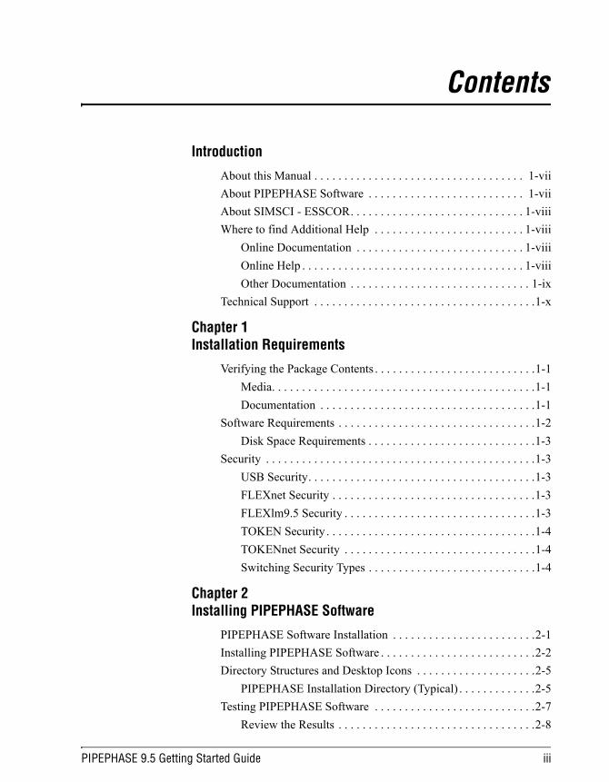
Contents

Introduction

About this Manual . . . . . . . . . . . . . . . . . . . . . . . . . . . . . . . . . . . 1-viiAbout PIPEPHASE Software . . . . . . . . . . . . . . . . . . . . . . . . . . 1-viiAbout SIMSCI - ESSCOR. . . . . . . . . . . . . . . . . . . . . . . . . . . . . 1-viiiWhere to find Additional Help . . . . . . . . . . . . . . . . . . . . . . . . . 1-viii

Online Documentation . . . . . . . . . . . . . . . . . . . . . . . . . . . . 1-viiiOnline Help . . . . . . . . . . . . . . . . . . . . . . . . . . . . . . . . . . . . . 1-viiiOther Documentation . . . . . . . . . . . . . . . . . . . . . . . . . . . . . . 1-ix

Technical Support . . . . . . . . . . . . . . . . . . . . . . . . . . . . . . . . . . . . .1-x

Chapter 1Installation Requirements

Verifying the Package Contents . . . . . . . . . . . . . . . . . . . . . . . . . . .1-1Media. . . . . . . . . . . . . . . . . . . . . . . . . . . . . . . . . . . . . . . . . . . .1-1Documentation . . . . . . . . . . . . . . . . . . . . . . . . . . . . . . . . . . . .1-1

Software Requirements . . . . . . . . . . . . . . . . . . . . . . . . . . . . . . . . .1-2Disk Space Requirements . . . . . . . . . . . . . . . . . . . . . . . . . . . .1-3

Security . . . . . . . . . . . . . . . . . . . . . . . . . . . . . . . . . . . . . . . . . . . . .1-3USB Security. . . . . . . . . . . . . . . . . . . . . . . . . . . . . . . . . . . . . .1-3FLEXnet Security . . . . . . . . . . . . . . . . . . . . . . . . . . . . . . . . . .1-3FLEXlm9.5 Security . . . . . . . . . . . . . . . . . . . . . . . . . . . . . . . .1-3TOKEN Security . . . . . . . . . . . . . . . . . . . . . . . . . . . . . . . . . . .1-4TOKENnet Security . . . . . . . . . . . . . . . . . . . . . . . . . . . . . . . .1-4Switching Security Types . . . . . . . . . . . . . . . . . . . . . . . . . . . .1-4

Chapter 2Installing PIPEPHASE Software

PIPEPHASE Software Installation . . . . . . . . . . . . . . . . . . . . . . . .2-1Installing PIPEPHASE Software . . . . . . . . . . . . . . . . . . . . . . . . . .2-2Directory Structures and Desktop Icons . . . . . . . . . . . . . . . . . . . .2-5

PIPEPHASE Installation Directory (Typical) . . . . . . . . . . . . .2-5Testing PIPEPHASE Software . . . . . . . . . . . . . . . . . . . . . . . . . . .2-7

Review the Results . . . . . . . . . . . . . . . . . . . . . . . . . . . . . . . . .2-8

PIPEPHASE 9.5 Getting Started Guide iii

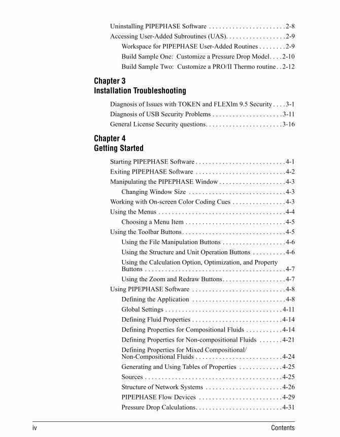
Uninstalling PIPEPHASE Software . . . . . . . . . . . . . . . . . . . . . . . 2-8Accessing User-Added Subroutines (UAS). . . . . . . . . . . . . . . . . . 2-9

Workspace for PIPEPHASE User-Added Routines . . . . . . . . 2-9Build Sample One: Customize a Pressure Drop Model. . . . 2-10Build Sample Two: Customize a PRO/II Thermo routine . . 2-12

Chapter 3Installation Troubleshooting

Diagnosis of Issues with TOKEN and FLEXlm 9.5 Security . . . . 3-1Diagnosis of USB Security Problems . . . . . . . . . . . . . . . . . . . . . 3-11General License Security questions. . . . . . . . . . . . . . . . . . . . . . . 3-16

Chapter 4Getting Started

Starting PIPEPHASE Software . . . . . . . . . . . . . . . . . . . . . . . . . . . 4-1Exiting PIPEPHASE Software . . . . . . . . . . . . . . . . . . . . . . . . . . . 4-2Manipulating the PIPEPHASE Window . . . . . . . . . . . . . . . . . . . . 4-3

Changing Window Size . . . . . . . . . . . . . . . . . . . . . . . . . . . . . 4-3Working with On-screen Color Coding Cues . . . . . . . . . . . . . . . . 4-3Using the Menus . . . . . . . . . . . . . . . . . . . . . . . . . . . . . . . . . . . . . . 4-4

Choosing a Menu Item . . . . . . . . . . . . . . . . . . . . . . . . . . . . . . 4-5Using the Toolbar Buttons . . . . . . . . . . . . . . . . . . . . . . . . . . . . . . . 4-5

Using the File Manipulation Buttons . . . . . . . . . . . . . . . . . . . 4-6Using the Structure and Unit Operation Buttons . . . . . . . . . . 4-6Using the Calculation Option, Optimization, and Property Buttons . . . . . . . . . . . . . . . . . . . . . . . . . . . . . . . . . . . . . . . . . . 4-7Using the Zoom and Redraw Buttons. . . . . . . . . . . . . . . . . . . 4-7

Using PIPEPHASE Software . . . . . . . . . . . . . . . . . . . . . . . . . . . . 4-8Defining the Application . . . . . . . . . . . . . . . . . . . . . . . . . . . . 4-8Global Settings . . . . . . . . . . . . . . . . . . . . . . . . . . . . . . . . . . . 4-11Defining Fluid Properties . . . . . . . . . . . . . . . . . . . . . . . . . . . 4-14Defining Properties for Compositional Fluids . . . . . . . . . . . 4-14Defining Properties for Non-compositional Fluids . . . . . . . 4-21Defining Properties for Mixed Compositional/Non-Compositional Fluids . . . . . . . . . . . . . . . . . . . . . . . . . . 4-24Generating and Using Tables of Properties . . . . . . . . . . . . . 4-25Sources . . . . . . . . . . . . . . . . . . . . . . . . . . . . . . . . . . . . . . . . . 4-25Structure of Network Systems . . . . . . . . . . . . . . . . . . . . . . . 4-26PIPEPHASE Flow Devices . . . . . . . . . . . . . . . . . . . . . . . . . 4-29Pressure Drop Calculations. . . . . . . . . . . . . . . . . . . . . . . . . . 4-31

iv Contents

Equipment Items . . . . . . . . . . . . . . . . . . . . . . . . . . . . . . . . . .4-38Heat Transfer Calculations . . . . . . . . . . . . . . . . . . . . . . . . . .4-41Sphering or Pigging. . . . . . . . . . . . . . . . . . . . . . . . . . . . . . . .4-42Reservoirs and Inflow Performance Relationships . . . . . . . .4-42Production Planning and Time-Stepping . . . . . . . . . . . . . . .4-43Subsurface Networks and Multiple Completion Modeling .4-45Case Studies . . . . . . . . . . . . . . . . . . . . . . . . . . . . . . . . . . . . .4-48Nodal Analysis . . . . . . . . . . . . . . . . . . . . . . . . . . . . . . . . . . .4-50

Starting the PIPEPHASE Results Access System (RAS) . . . . . .4-54Starting the PIPEPHASE Excel Report . . . . . . . . . . . . . . . . . . . .4-56

Chapter 5Tutorial

Introduction . . . . . . . . . . . . . . . . . . . . . . . . . . . . . . . . . . . . . . . . . .5-1Problem Description . . . . . . . . . . . . . . . . . . . . . . . . . . . . . . . . . . .5-1Building the Network. . . . . . . . . . . . . . . . . . . . . . . . . . . . . . . . . . .5-3Entering Optimization Data . . . . . . . . . . . . . . . . . . . . . . . . . . . . .5-20Specifying Print Options . . . . . . . . . . . . . . . . . . . . . . . . . . . . . . .5-28Running the Simulation . . . . . . . . . . . . . . . . . . . . . . . . . . . . . . . .5-29Viewing and Plotting Results. . . . . . . . . . . . . . . . . . . . . . . . . . . .5-30Using the RAS to Plot Results . . . . . . . . . . . . . . . . . . . . . . . . . . .5-31Generate and View Excel Report . . . . . . . . . . . . . . . . . . . . . . . . .5-34Including Operating Costs . . . . . . . . . . . . . . . . . . . . . . . . . . . . . .5-35

Index

PIPEPHASE 9.5 Getting Started Guide v

vi Contents

Introduction

About this ManualThe PIPEPHASE™ Getting Started Guide provides an introduction to PIPEPHASE software. It describes how the interface modules work and includes a step-by-step tutorial to guide you through a PIPEPHASE example optimization problem. Also covered in this guide is PIPEPHASE Keywords. An outline of this guide is pro-vided below. This manual will guide you through the installation of

PIPEPHASE software. An outline of the manual is provided below.

About PIPEPHASE SoftwarePIPEPHASE software is a simulation program which predicts steady-state pressure, temperature, and liquid holdup profiles in wells, flowlines, gathering systems, and other linear or network configurations of pipes, wells, pumps, compressors, separators, and other facilities. The fluid types that PIPEPHASE software can han-dle include liquid, gas, steam, and multiphase mixtures of gas and liquid.

Introduction Introduces the manual, the program, and SIMSCI.

Chapter 1 Installation Requirements

Provides you with the installation and security requirements.

Chapter 2 Installing PIPEPHASE

Describes how to install PIPEPHASE software.

Chapter 3 Installation Trou-bleshooting

Addresses some of the problems you may encounter while installing PIPEPHASE software.

Chapter 4 Getting Started Explains how to use PIPEPHASE software.

Chapter 5 Tutorial Provides a step-by-step tutorial for the optimiza-tion of an off-line pipeline design.

PIPEPHASE 9.5 Getting Started Guide vii

Several special capabilities have also been designed into PIPEPHASE software including well analysis with inflow perfor-mance; gas lift analysis; pipeline sphering; and sensitivity (nodal) analysis. These additions extend the range of the PIPEPHASE application so that the full range of pipeline and piping network problems can be solved.

About SIMSCI - ESSCORSimSci-Esscor, a business unit of Invensys Systems, Inc., is a leader in the development and deployment of industrial process simulation software and systems for a variety of industries, including oil and gas production, petroleum refining, petrochemical and chemical manufacturing, electrical power generation, mining, pulp and paper, and engineering and construction. Supporting more than 750 client companies in over 70 countries, SimSci-Esscor solutions enable cli-ents to minimize capital requirements, optimize facility perfor-mance, and maximize return on investment.

For more information, visit SimSci-Esscor Web site at http://www.simsci-esscor.com.

Where to find Additional Help

Online DocumentationPIPEPHASE online documentation is provided in the form of .PDF

files that are most conveniently viewed using Adobe Acrobat® Reader 7.0.5 or Acrobat Exchange 5.0. Online manuals are stored in the Manuals directory and they remain on the CD when you install the program. To access these files, open the PIPEPHASE ONLINE HELP.CHM file in the HLP directory and click the appropriate link to navigate to the corresponding PDF.

Online HelpPIPEPHASE comes with online Help, a comprehensive online ref-erence tool that accesses information quickly. In Help, commands, features, and data fields are explained in easy steps. Answers are available instantly, online, while you work. You can access the elec-tronic contents for Help by selecting Help/Contents from the menu bar. Context-sensitive help is accessed using the F1 key or the What’s This? button by placing the cursor in the area in question. A Road Map to Online Help will be displayed where you can select the help document you wish to view. From the desired online help

viii Introduction

document you can do a search for the desired topic. If you chose a .CHM file, you can search by selecting Help/Search from the menu bar. If you chose a .PDF formatted document, you can use all the available Acrobat Reader search features to find the topic of inter-est. Please refer to Acrobat Reader on-line help for information concerning Acrobat Reader features.

Other DocumentationThe table below outlines the other existing PIPEPHASE documen-tation available in a hardcopy form.

Where to Find Additional HelpIf you want to... See...

Quickly learn how to simulate a simple flowsheet using PIPEPHASE software

This document

Obtain detailed information on the capabilities and use of PIPEPHASE software

This document

Learn how to install PIPEPHASE software This document

Obtain basic information on PIPEPHASE keywords

PIPEPHASE Keyword Manual

See simulation examples PIPEPHASE Application Briefs

To learn more on Well and Surface Models Well and Surface Examples

Obtain detailed information on using PIPEPHASE software w/ NETOPT® module

NETOPT User’s Guide

Obtain detailed information on using PIPEPIPEPHASE software w/ TACITE®

module

TACITE User’s Guide

Obtain basic information on PIPEPHASE calculation methods

Online Help

Obtain detailed information of component and thermodynamic properties

SIMSCI Component and Thermodynamic Data Input Manual

PIPEPHASE 9.5 Getting Started Guide ix

Technical SupportIf you have any questions regarding program use or the interpretation of program output, contact the nearest SimSci-Esscor Technical Support Center from the following address list, or contact your local SimSci-Esscor representative.

To expedite your request for assistance, please have the following information available when you call:

■ A description of the problem

■ The installation CD and printed documentation available

■ The type of computer you are using

■ The amount of free disk space available on the disk where PIPEPHASE software is installed

■ The actions you were taking when the problem occurred

■ The error messages that appear on your screen and any other symptoms

x Introduction

Authorized SimSci- Esscor Technical Support CentersSupport Center Address Tel/Fax/Internet

USA Invensys Process Systems (SimSci-Esscor)10900 Equity DriveHouston, TX 77041

Tel: + 1 800 SIMSCI 1+ 1 713 329 8584

Fax: + 1 713 329 1700E-mail: [email protected]

USA East Coast Invensys Process Systems (SimSci-Esscor)Gateway Corporate Center, Suite 304, 223 Wilmington-West Chester Pike,Chaddsford, PA 19317

Tel: + 1 800 SIMSCI 1+ 1 484 840 9407

Fax: + 1 484 480 9499E-mail: [email protected]

USA West Coast Invensys SimSci-Esscor,26561 Rancho Parkway South, Suite 100,Lake Forest, CA 92630

Tel: + 1 800 SIMSCI 1Fax: + 1949 455 8154E-mail: [email protected]

Mexico Invensys Systems Mexico S.AAmargura # 60 Col. Parques de la Herradura,Huixquilucan, Edo.de, 52786

Tel: + 52 55 52 63 01 76Fax:+ 52 55 52 63 01 60E-mail:[email protected]

Canada Invensys SIMSCI-ESSCOR,7665 - 10th Street NE,Calgary T2E8X2

Tel: + 403-617-6220 (Cell)Fax: + 403-274-8651E-mail: [email protected]

Argentina Invensys Systems Argentina Inc.Nunez 4334Buenos Aires (Argentina) C1430AND

Tel: + 54 11 6345 2100Fax: + 54 11 6345 2111E-mail: [email protected]

Italy Invensys Systems Italia S.p.AVia Carducci, 126Sesto San Giovanni (MI) 20100, Italia


Venezuela Invensys Systems VenezuelaTorre Delta Piso 12, Av.Francisco de MirandaAltamira, Caracas 1060

Tel: + 58 212 267 5868 ext. 282Fax: + 58 212 2670964E-mail: [email protected]

Brazil Invensys Systems Brasil Ltda.Av. Chibaras, 75 - MoemaSao Paulo, SP O 4076 - 000

Tel:+ 55 11 2844 0201/291Fax: + 55 11 2844 0341E-mail: [email protected]

Germany Invensys Systems GmbHWilly- Brandt- Platz, 6Mannheim, 68161

Tel: + 49(0)89 44419650E-mail: [email protected]

Australia and New Zealand Invensys Performance SolutionsLevel 2-4, 810 Elizabeth StreetSydney 2017, Australia

Tel: + 61 2 8396 3626Fax:+ 61 2 8396 3604E-mail: [email protected]

Japan Invensys Systems Japan8th Fl. Suzuebaydium, 1-15-1 Kaigan,Minato-ku, Tokyo 105-0022 Japan

Tel: + 81 3 6450 1095Fax:+ 81 3 5408 9220E-mail: [email protected]

Middle East Invensys ME DubaiPO Box 61495Jebel Ali Free Zone, Dubai


Asia - Pacific Invensys Software Systems (s) Pte. Ltd.15, Changi Business ParkCentral 1Singapore 486057

Tel: + 65 6829 8643Fax: + 65 6829 8202E-mail: [email protected]

United Kingdom Invensys Systems (UK) LimitedThe Genesis Centre, Birchwood Science Park,Birchwood, WarringtonUnited Kingdom WA3 7BH

Tel: + 44 (0) 1925 811469Fax: + 44 (0) 1925 838509E-mail: [email protected]

China Invensys Process Systems (China),No. 211, Huancheng Road East, Fengpu Industrial Park, Shanghai 201400

Tel: + 86 21 3718 0000 ext. 5912Fax: + 86 10 8458 4521E-mail: [email protected]

Colombia Invensys Systems LA ColombiaCalle 100 # 36-39 Int. 4-203, Bucaramanga, SDER

Tel: + 57 1 3136360E-mail: [email protected]

PIPEPHASE 9.5 Getting Started Guide xi

Korea Invensys Korea Simsci-Esscor6F, Dongsung B/D, 17-8, Yeouidodong,Seoul, 150-874

Tel: + 82-32-540-0665Fax: + 82-32-542-3778E-mail: [email protected]

Authorized SimSci- Esscor Technical Support Centers

xii Introduction

Chapter 1Installation Requirements

This chapter provides a list of the PIPEPHASE package contents, the installation requirements, and an outline of the hardware and software requirements for running PIPEPHASE software.

Verifying the Package ContentsThis section describes the contents of your release package.

MediaPIPEPHASE software is provided on a single CD. The TACITE Transient Module and the NETOPT Optimizer Module are also included on the PIPEPHASE product CD. SimSci-Esscor FLEXlm™ server application installation program is provided on a separate CD.

DocumentationA list of PIPEPHASE documents is provided below. If you need a manual that is not included in your installation package or add-on package, contact Technical Support to request it.

■ PIPEPHASE Getting Started Guide (This document)

■ PIPEPHASE Keyword Manual

■ Release Notes

■ Other documentation as required:

● NETOPT User’s Guide

● TACITE User’s GuideA complete set of online documentation is provided for each product.

PIPEPHASE 9.5 Getting Started Guide 1-1

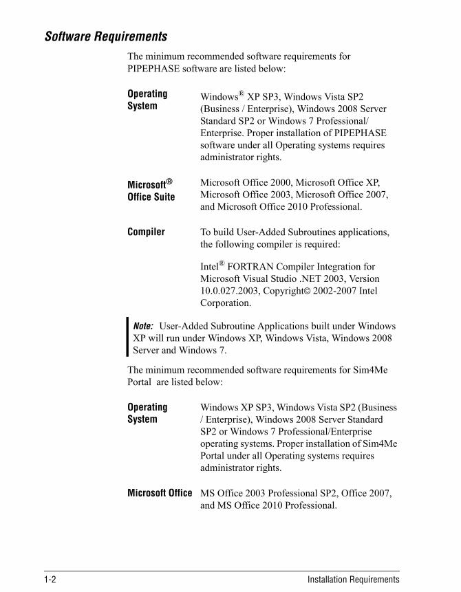
Software RequirementsThe minimum recommended software requirements for PIPEPHASE software are listed below:

The minimum recommended software requirements for Sim4Me Portal are listed below:

OperatingSystem

Windows® XP SP3, Windows Vista SP2 (Business / Enterprise), Windows 2008 Server Standard SP2 or Windows 7 Professional/Enterprise. Proper installation of PIPEPHASE software under all Operating systems requires administrator rights.

Microsoft® Office Suite

Microsoft Office 2000, Microsoft Office XP, Microsoft Office 2003, Microsoft Office 2007, and Microsoft Office 2010 Professional.

Compiler To build User-Added Subroutines applications, the following compiler is required:

Intel® FORTRAN Compiler Integration for Microsoft Visual Studio .NET 2003, Version 10.0.027.2003, Copyright© 2002-2007 Intel Corporation.

Note: User-Added Subroutine Applications built under Windows XP will run under Windows XP, Windows Vista, Windows 2008 Server and Windows 7.

OperatingSystem

Windows XP SP3, Windows Vista SP2 (Business / Enterprise), Windows 2008 Server Standard SP2 or Windows 7 Professional/Enterprise operating systems. Proper installation of Sim4Me Portal under all Operating systems requires administrator rights.

Microsoft Office MS Office 2003 Professional SP2, Office 2007, and MS Office 2010 Professional.

1-2 Installation Requirements

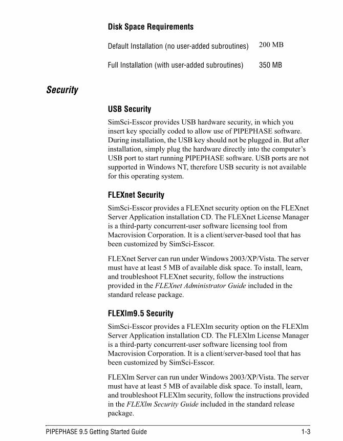
Disk Space Requirements

Security

USB SecuritySimSci-Esscor provides USB hardware security, in which you insert key specially coded to allow use of PIPEPHASE software. During installation, the USB key should not be plugged in. But after installation, simply plug the hardware directly into the computer’s USB port to start running PIPEPHASE software. USB ports are not supported in Windows NT, therefore USB security is not available for this operating system.

FLEXnet SecuritySimSci-Esscor provides a FLEXnet security option on the FLEXnet Server Application installation CD. The FLEXnet License Manager is a third-party concurrent-user software licensing tool from Macrovision Corporation. It is a client/server-based tool that has been customized by SimSci-Esscor.

FLEXnet Server can run under Windows 2003/XP/Vista. The server must have at least 5 MB of available disk space. To install, learn, and troubleshoot FLEXnet security, follow the instructions provided in the FLEXnet Administrator Guide included in the standard release package.

FLEXlm9.5 SecuritySimSci-Esscor provides a FLEXlm security option on the FLEXlm Server Application installation CD. The FLEXlm License Manager is a third-party concurrent-user software licensing tool from Macrovision Corporation. It is a client/server-based tool that has been customized by SimSci-Esscor.

FLEXlm Server can run under Windows 2003/XP/Vista. The server must have at least 5 MB of available disk space. To install, learn, and troubleshoot FLEXlm security, follow the instructions provided in the FLEXlm Security Guide included in the standard release package.

Default Installation (no user-added subroutines) 200 MB

Full Installation (with user-added subroutines) 350 MB


TOKEN SecuritySimSci-Esscor provides a TOKEN security option on the FLEXlm Server 9.5 Application installation CD. The FLEXlm License Manager is a third-party concurrent-user software licensing tool from Macrovision Corporation. It is a client/server-based tool that has been customized by SimSci-Esscor.

For detailed information please refer to the SIM4ME License Security User Guide available in the Pphase95\Manuals\PIPEPHASE Getting Started Guide folder.

TOKENnet SecuritySimSci-Esscor provides a TOKENnet security option on the FLEXnet Server Application installation CD. The FLEXnet License Manager is a third-party concurrent-user software licensing tool from Macrovision Corporation. It is a client/server-based tool that has been customized by SimSci-Esscor.

For detailed information please refer to the SIM4ME License Secu-rity User Guide available in the Pphase95\Manuals\PIPEPHASE Getting Started Guide folder.

Switching Security Types

To switch to USB security:

■ Open the pipephase.ini file found in the user directory.

■ Find the section entitled [wss_Security] and set Type=USB.

■ Save the file and exit.

To switch to FLEXNET11 security:


■ Find the section entitled [wss_Security] and set Type=FLXNET11.


■ Set system environment variable as IPASSI_LICENSE_FILE=@{FLEXnet server machine name}

■ Reboot your computer so the changes to your security environment will be correctly configured.


To switch to FLEXlm9.5 security:


■ Find the section entitled [wss_Security] and set Type=FLXLM95.


■ Set the system environment variable as IPASSI_LICENSE_FILE=@{FLEXlm server machine name}

■ Reboot your computer so the changes to your security environment will be correctly configured.

To switch to TOKEN security:


■ Find the section entitled [wss_Security] and set Type=TOKEN.


■ Set the system environment variable as IPASSI_LICENSE_FILE=@{FLEXlm server machine name}

■ Reboot your computer, so the changes to your security environment will be correctly configured.

To switch to TOKENnet security:


■ Find the section entitled [wss_Security] and set Type=TOKEN-net


■ Set the system environment variable as IPASSI_LICENSE_FILE=@{FLEXnet server machine name}

■ Reboot your computer, so the changes to your security environ-ment will be correctly configured.



Chapter 2Installing PIPEPHASE Software

This chapter explains how to install PIPEPHASE software as a standalone version.

PIPEPHASE Software InstallationThere are two installation options for the PIPEPHASE software:

When installing PIPEPHASE software, you also have the option to install the TACITE Transient module and/or the NETOPT Optimizer module and/or SIM4ME Portal 2.0.1. If you do not have license and would like to add-on one or all of these modules, please contact your SimSci-Esscor representative for details.

Typical - This option installs both the GUI and the calculation portions of PIPEPHASE software directly to your PC.

Custom - This option allows you to customize your installation by selecting the User Added files with PIPEPHASE software.

Note: PC user-added subroutines require a custom installation.


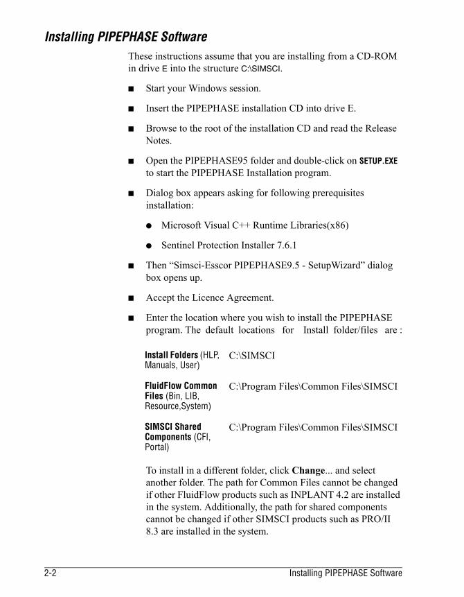
Installing PIPEPHASE SoftwareThese instructions assume that you are installing from a CD-ROM in drive E into the structure C:\SIMSCI.

■ Start your Windows session.

■ Insert the PIPEPHASE installation CD into drive E.

■ Browse to the root of the installation CD and read the Release Notes.

■ Open the PIPEPHASE95 folder and double-click on SETUP.EXE to start the PIPEPHASE Installation program.

■ Dialog box appears asking for following prerequisites installation:

● Microsoft Visual C++ Runtime Libraries(x86)

● Sentinel Protection Installer 7.6.1

■ Then “Simsci-Esscor PIPEPHASE9.5 - SetupWizard” dialog box opens up.

■ Accept the Licence Agreement.

■ Enter the location where you wish to install the PIPEPHASE program. The default locations for Install folder/files are :

To install in a different folder, click Change... and select another folder. The path for Common Files cannot be changed if other FluidFlow products such as INPLANT 4.2 are installed in the system. Additionally, the path for shared components cannot be changed if other SIMSCI products such as PRO/II 8.3 are installed in the system.

Install Folders (HLP, Manuals, User)

C:\SIMSCI

FluidFlow Common Files (Bin, LIB, Resource,System)

C:\Program Files\Common Files\SIMSCI

SIMSCI Shared Components (CFI, Portal)

C:\Program Files\Common Files\SIMSCI

2-2 Installing PIPEPHASE Software

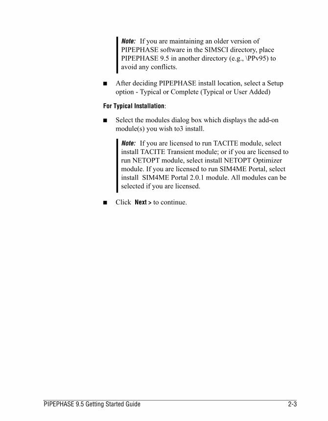
■ After deciding PIPEPHASE install location, select a Setup option - Typical or Complete (Typical or User Added)

For Typical Installation:

■ Select the modules dialog box which displays the add-on module(s) you wish to3 install.

■ Click Next > to continue.

Note: If you are maintaining an older version of PIPEPHASE software in the SIMSCI directory, place PIPEPHASE 9.5 in another directory (e.g., \PPv95) to avoid any conflicts.

Note: If you are licensed to run TACITE module, select install TACITE Transient module; or if you are licensed to run NETOPT module, select install NETOPT Optimizer module. If you are licensed to run SIM4ME Portal, select install SIM4ME Portal 2.0.1 module. All modules can be selected if you are licensed.


■ The Security Option dialog box appears. Select one of the four security options:

● If you chose FLXNET11, FLEXlm9.5, or Token, specify the prospective IPASSI FLEXlm server(s) (e.g., @server1; @server2) to guide PIPEPHASE software to find the FLEXlm server. Click Next > to continue.

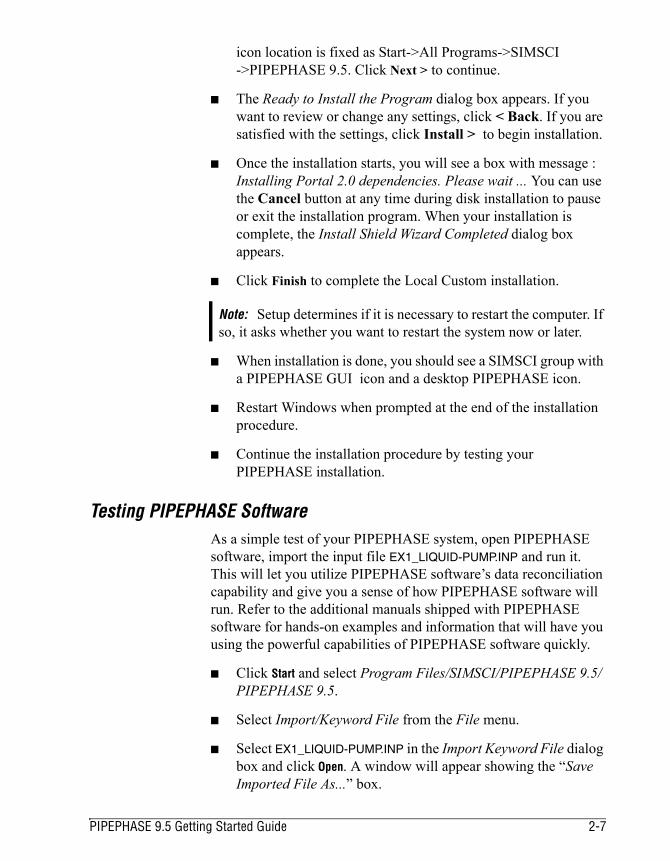
■ Then a dialog box appears to select the options of creating a shortcut on the Desktop and/or the Quick launch bar. Pipephase icon location is fixed as Start->All Programs->SIMSCI->PIPEPHASE 9.5. Click Next > to continue.

■ The Ready to Install the Program dialog box appears. If you want to review or change any settings, click < Back. If you are satisfied with the settings, click Install > to begin installation.

■ Once the installation starts, you will see a box with message : Installing Portal 2.0.1 dependencies. Please wait ... You can use the Cancel button at any time during disk installation to pause or exit the installation program. When your installation is complete, the Install Shield Wizard Completed dialog box appears.

FLEXlm9.5 Server Allows PIPEPHASE software to go beyond the current machine to obtain licenses from another machine (FLEXlm9.5 security server machine) on the network.

FLXNET11 Server Allows PIPEPHASE software to go beyond the current machine to obtain licenses from another machine (FLXNET11 security server machine) on the network.

USB Utilizes a USB hardware key attached to the USB port on the back of the current machine for licensing purposes. Using this type, PIPEPHASE software will only search this hardware key for license(s).

Token Allows PIPEPHASE software to go beyond the current machine to obtain licenses from a Token server on the network.


■ Click Finish to complete the Local Typical installation.

You should now test your PIPEPHASE installation. Proceed to the Testing PIPEPHASE section for more information.

Directory Structures and Desktop Icons

PIPEPHASE Installation Directory (Typical)The Typical Installation will set up all PIPEPHASE files under the directories shown below:

C:\Program Files\Common Files\SIMSCI\FluidFlow95\Bin [Program executable files]

C:\Program Files\Common Files\SIMSCI\FluidFlow95\LIB [Component library directory]

C:\Program Files\Common Files\SIMSCI\FluidFlow95\SYSTEM [PIPEPHASE system files]

C:\Program Files\PFE32 [Text editor]

C:\SIMSCI\Pphase95\User [PIPEPHASE user directory]

C:\SIMSCI\Pphase95\Manuals [PIPEPHASE Manuals]

C:\SIMSCI\Pphase95\HLP [PIPEPHASE HLP Manuals]

C:\Program Files\Common Files\SIMSCI\FluidFlow95\RESOURCE [GUI bitmaps and icon files]

C:\Program Files\Common Files\SIMSCI\SIM4MEPortal201 [SIM4ME Portal files]C:\Program Files\Common Files\ [SIMSCI Common

SIMSCI\SIMSCICFI40 [Framework Files]

A typical installation creates the following four icons:

● PIPEPHASE 9.5 Software

● PIPEPHASE 9.5 Online Help

● SIM4ME Portal

For Custom Installation:

■ Choose the components you wish to install.

● If you plan to link your own user-added subroutines into PIPEPHASE software, select the User-Added Files option.

Note: Setup determines if it is necessary to restart the computer. If so, it asks whether you want to restart the system now or later.


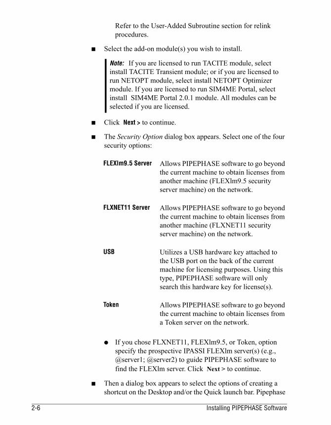
Refer to the User-Added Subroutine section for relink procedures.

■ Select the add-on module(s) you wish to install.

■ Click Next > to continue.

■ The Security Option dialog box appears. Select one of the four security options:

● If you chose FLXNET11, FLEXlm9.5, or Token, option specify the prospective IPASSI FLEXlm server(s) (e.g., @server1; @server2) to guide PIPEPHASE software to find the FLEXlm server. Click Next > to continue.

■ Then a dialog box appears to select the options of creating a shortcut on the Desktop and/or the Quick launch bar. Pipephase

Note: If you are licensed to run TACITE module, select install TACITE Transient module; or if you are licensed to run NETOPT module, select install NETOPT Optimizer module. If you are licensed to run SIM4ME Portal, select install SIM4ME Portal 2.0.1 module. All modules can be selected if you are licensed.

FLEXlm9.5 Server Allows PIPEPHASE software to go beyond the current machine to obtain licenses from another machine (FLEXlm9.5 security server machine) on the network.

FLXNET11 Server Allows PIPEPHASE software to go beyond the current machine to obtain licenses from another machine (FLXNET11 security server machine) on the network.

USB Utilizes a USB hardware key attached to the USB port on the back of the current machine for licensing purposes. Using this type, PIPEPHASE software will only search this hardware key for license(s).

Token Allows PIPEPHASE software to go beyond the current machine to obtain licenses from a Token server on the network.


icon location is fixed as Start->All Programs->SIMSCI->PIPEPHASE 9.5. Click Next > to continue.

■ The Ready to Install the Program dialog box appears. If you want to review or change any settings, click < Back. If you are satisfied with the settings, click Install > to begin installation.

■ Once the installation starts, you will see a box with message : Installing Portal 2.0 dependencies. Please wait ... You can use the Cancel button at any time during disk installation to pause or exit the installation program. When your installation is complete, the Install Shield Wizard Completed dialog box appears.

■ Click Finish to complete the Local Custom installation.

■ When installation is done, you should see a SIMSCI group with a PIPEPHASE GUI icon and a desktop PIPEPHASE icon.

■ Restart Windows when prompted at the end of the installation procedure.

■ Continue the installation procedure by testing your PIPEPHASE installation.

Testing PIPEPHASE SoftwareAs a simple test of your PIPEPHASE system, open PIPEPHASE software, import the input file EX1_LIQUID-PUMP.INP and run it. This will let you utilize PIPEPHASE software’s data reconciliation capability and give you a sense of how PIPEPHASE software will run. Refer to the additional manuals shipped with PIPEPHASE software for hands-on examples and information that will have you using the powerful capabilities of PIPEPHASE software quickly.

■ Click Start and select Program Files/SIMSCI/PIPEPHASE 9.5/PIPEPHASE 9.5.

■ Select Import/Keyword File from the File menu.

■ Select EX1_LIQUID-PUMP.INP in the Import Keyword File dialog box and click Open. A window will appear showing the “Save Imported File As...” box.

Note: Setup determines if it is necessary to restart the computer. If so, it asks whether you want to restart the system now or later.


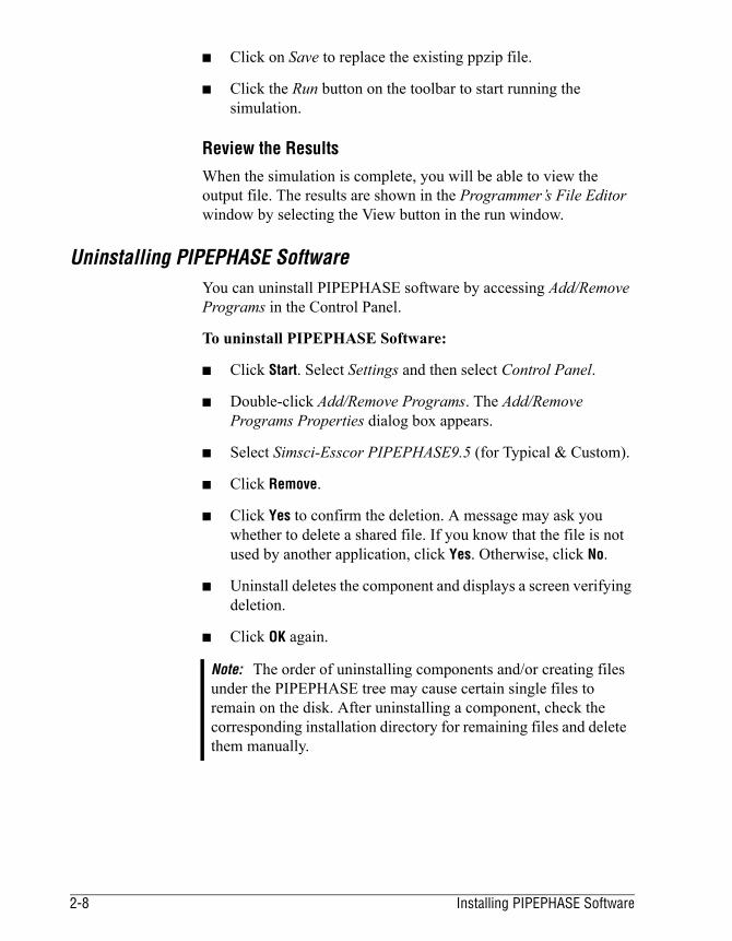
■ Click on Save to replace the existing ppzip file.

■ Click the Run button on the toolbar to start running the simulation.

Review the ResultsWhen the simulation is complete, you will be able to view the output file. The results are shown in the Programmer’s File Editor window by selecting the View button in the run window.

Uninstalling PIPEPHASE SoftwareYou can uninstall PIPEPHASE software by accessing Add/Remove Programs in the Control Panel.

To uninstall PIPEPHASE Software:

■ Click Start. Select Settings and then select Control Panel.

■ Double-click Add/Remove Programs. The Add/Remove Programs Properties dialog box appears.

■ Select Simsci-Esscor PIPEPHASE9.5 (for Typical & Custom).

■ Click Remove.

■ Click Yes to confirm the deletion. A message may ask you whether to delete a shared file. If you know that the file is not used by another application, click Yes. Otherwise, click No.

■ Uninstall deletes the component and displays a screen verifying deletion.

■ Click OK again.

Note: The order of uninstalling components and/or creating files under the PIPEPHASE tree may cause certain single files to remain on the disk. After uninstalling a component, check the corresponding installation directory for remaining files and delete them manually.


Accessing User-Added Subroutines (UAS)You can choose to install the directories for UAS during the standard installation procedures. See the instructions earlier in this chapter.

Building and Using PIPEPHASE UAS

User-Added Subroutines written in FORTRAN can be integrated into PIPEPHASE by creating a new D_MAINONE.DLL module. User- Added Subroutines for the PRO/II thermodynamics can be integrated into PIPEPHASE by creating a new FFPESMainDLL.DLL.

The User-Added Subroutines must be compiled and linked using Intel Visual FORTRAN (or IVF) for Windows 2003/XP. Refer to the Hardware/Software Requirements section of "Chapter 1" for information concerning the version of IVF required for this release of PIPEPHASE.

The build procedures outlined in this chapter assumes that you are familiar with the currently supported versions of the Windows OS and IVF. If you already have IVF installed on your computer, you can find information on setting up your computer's environment in the batch file located at c:\program files\devstudio\df\bin\dfvars.

This manual does not contain instructions on writing the FORTRAN subroutines or using IVF. For information on using IVF, see the Compaq Visual FORTRAN Programmer's Guide.

Workspace for PIPEPHASE User-Added RoutinesThe workspace C:\SIMSCI\PPHASE95\USERADD\Makewsp\MAKEWSP.SLN contains several projects, listed below in the order most commonly used:

Note: These instructions assume that you have installed the PIPEPHASE UAS files in the default directory structure, C:\SIMSCI\PPHASE95\USERADD. Modify the paths indicated in the procedure below if you have installed the routine in a directory structure other than the default structure.


** Refer to the PIPEPHASE documentation for information regarding PIPEPHASE User-Added capabilities.

Build Sample One: Customize a Pressure Drop Model In this sample build procedure, we will integrate the sample UAS routine HUSER1.FOR into D_MAINONE.DLL.

First you must open the development project:

■ Start IVF by selecting it from the Start menu.

■ Select the Open Workspace option from the menu.

■ Select project \SIMSCI\PPHASE95\USERADD\MAKEWSP\MAKESP.SLN

■ Set the active project to D_MAINONE by selecting Set Active Project from the Project menu.

Next you must add the file HUSER1.FOR into project:

■ Select the folder "CLIENT USER FILES" and use the right mouse button to select the "Add Files to Folder" option.

■ Add the file \SIMSCI\PPHASE95\USERADD\USERSRC\HUSER1.FOR. (If this file is already in the project, a message will be displayed.)

Table 2-1: Work Space for PIPEPHASE User Added RoutinesProject Description Build Products

D_MAINONE Project used to update PIPEPHASE user-added routines (i.e. HUSER1.FOR)

D_MAINONE.DLL

MAINONE_CPP Main program entry point provided for debugging purposes

MAINONE.EXE

FFPESMAINDLL Project used to update PRO/II thermo user-added routines **(i.e. HUSER1.FOR)

FFPESMainDLL.DLL

MAINTI Main program for thermo preprocessor provided for debugging purposes

MAINTI.EXE

Note: Build products must be copied into the C:\PROGRAM FILES\COMMON FILES\SIMSCI\FLUIDFLOW95\BIN directory. You should save the original products into another directory in case you want to go back to the standard release version.


■ Click OK to close the window and update the project file.

Next you can update the code and build D_MAINONE.DLL:

■ Modify the user added routine. For example increase the frictional pressure drop by 10% (PGF = PGF*1.1).

■ Select the "Win 32 Release" version.

■ Select the Rebuild All option from the Build menu. This builds D_MAINONE.DLL in directory \SIMSCI\PPHASE95\USERADD\MAKEWSP. Copy this file to the C:\PROGRAM FILES\COMMON FILES\SIMSCI\FLUIDFLOW95\BIN directory.

Now you can verify the UAS in the build:

■ Run file \SIMSCI\PPHASE95\USERADD\USERINP\HUSER.INP and compare the results to file HUSER.CHK. View the Node Summary and verify that the pressure drop has changed as expected.

You may also use the MAINONE_CPP project for debugging.

■ Repeat the build procedures for D_MAINONE.DLL but select the "Win 32 Debug" option. D_MAINONE.DLL will still be built directory \SIMSCI\PPHASE95\USERADD\MAKEWSP. Copy this file to the C:\PROGRAM FILES\COMMON FILES\SIMSCI\FLUIDFLOW95\BIN directory.

■ Now set the active project to MAINONE_CPP by selecting Set Active Project from the Project menu.

■ Select the "Win 32 Debug" version.

■ Select the Rebuild All option from the Build menu. IVF will build the MAINONE.EXE in the directory \SIMSCI\PPHASE95\USERADD\MAKEWSP. Copy this file to the C:\PROGRAM FILES\COMMON FILES\SIMSCI\FLUIDFLOW95\BIN directory.


■ Set the debug options as follows:

■ Set a breakpoint in MAINONE_CPP at command to "Run Preprocessor" and run to this breakpoint.

■ Now you can set breakpoints in the user added routines and debug as normal.

Build Sample Two: Customize a PRO/II Thermo routine In this sample build procedure, we will integrate the sample UAS routine UKHS1.FOR into FFPESMainDLL.DLL.

First you must open the development project:

■ Start IVF by selecting it from the Start menu.

■ Select the Open Workspace option from the menu.

■ Select file C:\SIMSCI\PPHASE95\USERADD\MAKEWSP\MAKEWSP.SLN and click OK.

■ Set the active project to FFPESMainDLL by selecting Set Active Project from the Project menu.

Next, you must add the file UKHS1.FOR into the project:

■ Select the folder "CLIENT USER FILES" and use the right mouse button to select the "Add Files to Folder" option.

■ Add the file \SIMSCI\PPHASE95\USERADD\USERSRC\UKHS1.FOR. (If this file is already in the project, a message will be displayed.)

■ Click OK to close the window and update the project file.

Next you can update the code and build FFPESMainDLL.DLL:

■ Select the "Win 32 Release" version.

Executable for… C:\PROGRAM FILES\COMMON FILES\SIMSCI\FLUIDFLOW95\BIN\MAINONE

Working Dir… C:\PROGRAM FILES\COMMON FILES\SIMSCI\FLUIDFLOW95\BIN

Program Arg…. /F=filename /D=\SIMSCI\PPHASE95\USER\ / I=\SIMSCI\PPHASE95\USER\ PIPEPHASE.INI


■ Modify the user added routine. For example, increase the liquid density by 10% (DENSE = DENSE*1.1).

■ Select the Rebuild All option from the Build menu. IVF will build the FFPESMainDLL.DLL module in the directory \SIMSCI\PPHASE95\USERADD\MAKEWSP. Copy this file to the C:\PROGRAM FILES\COMMON FILES\SIMSCI\FLUIDFLOW95\BIN directory.

Now you can verify the UAS build:

■ Run file \SIMSCI\PPHASE95\USERADD\USERINP\ETH_UAS.INP and compare the results to file ETH_UAS.CHK.

Note: To update the version identification to include the "UAS", you must rebuild D_MAINONE.DLL as described in the previous example.

Note: You may debug your routines by building this dll in debug mode as described in the previous example.



Chapter 3Installation Troubleshooting

This chapter addresses some of the more common support questions and problems related to TOKEN and FLEXlm 9.5 server, USB, and General License security.

If you are having problems installing this product, review this section. If you are unable to correct the problem, contact Technical Support located at your local SIMSCI Technical Support Center, as listed in Introduction.

Diagnosis of Issues with TOKEN and FLEXlm 9.5 SecurityStep 1 - Ensure that the FLEXlm server is working correctlyWhen encountering a licensing problem with TOKEN or FLEXlm 9.5 security, first ensure that the FLEXlm server is running without any errors. The TOKEN license server is actually a FLEXlm 9.x server, and the only difference between these two types of license servers lies in the license files, one being token-based (each product requires a specified number of tokens when used) and the other product-specific. Incidentally, only a 9.x FLEXlm server can manage a SimSci-Esscor TOKEN license file. There are two ways to verify that the FLEXlm server is running correctly.

The first way is to examine the FLEXlm server debug log file ipassi.log. This log file is by default located in the FLEXlm directory (C:\Program Files\IPASSI\Security\FLEXlm95 for FLEXlm 9.5) The actual location for this log file can be found from the FLEXlm lmtool.exe utility in the "Path to the debug log file" field on the "Config Services" tab (see figure below). Carefully go through the log file to see if there are any errors recorded in this log file.


Figure 3-1: LMTOOLS’ Config Services tab

Alternatively, after attempting to start the FLEXlm server, start the lmtools.exe utility, click on the "Server Status" button on the "Sever Status" tab, and then click the "Perform Status Enquiry" button (as shown in the Figure on the next page). Again, carefully go through the output text to find any error messages. Note that if you need to perform the server status enquiry multiple times, you can use "Edit->Clear Window" from the menu bar as this will clear the output text box for easy reading.

3-2 Installation Troubleshooting

Figure 3-2: Server Status Tab

If there are any error messages in the FLEXlm server log file or in the lmtool.exe "Server Status" output text window, try and take appropriate action to resolve the problem yourself.

Examples:

If you try to start the FLEXlm server on a license file not intended for the license server, you will get an authentication error. In this case, you will either need to install the license (and FLEXlm server) on the machine for which the license was generated, or contact [email protected] to issue you a license file for the machine on which the FLEXlm server is installed.

Another issue could be that the licenses themselves have expired. The expiry date can either be obtained by looking at the license file, ipassi.lic, or by clicking on the "Perform Diagnostics" button on the "Server Diags" tab. If the licenses have expired, then contact [email protected] to renew your licenses.

A further common error is that the FLEXlm server machine name, the second item on the SERVER line in the FLEXlm license file, is not stated correctly. An example of the server line, from a permanent license, is as follows:

SERVER miawa2ca 000874fe5ea8

Or for a temporary license:


SERVER ukfcra-g6fyq0j ANY

Note, for a temporary license the ANY, the third item on the SERVER line, must be retained.

If the machine name is correct in the SERVER line but the FLEXlm server is still not starting correctly, then use the IP address of the server machine instead of the machine name.

For errors that you cannot resolve yourself, contact your SimSci-Esscor technical support for assistance. When doing so, have the server log file available to send as this will aid in the troubleshooting.

Step 2 - Ensure that the application is using FLEXlm/TOKEN securityIf the FLEXlm server is up and running with the correct license, but there is still a problem launching the application due to a FLEXlm/TOKEN security error, then the focus should switch to the SimSci-Esscor application side. The second step in troubleshooting FLEXlm/TOKEN security is to verify if FLEXlm/TOKEN is indeed the active license security type. This selection of license security type is made in the main initialization file (*.ini) of the application. These files are usually named after the applications they control, such as PROII.ini, PIPEPHASE.ini, DATACON.ini, etc. The easiest way to locate these ini files is to search the application directory for the *.ini file that contains the string [wss_Security]. Once you identify the ini file, you need to open the file (Notepad will work fine for this) to see what the active security type is. Search for the Type statement in the [wss_Security] section. The active security Type statement is the one that does not have a semi-colon (;) in front of it. If FLEXlm/TOKEN is not the current active security type, you will need to comment out the current active type by placing a semi-colon at the beginning of that line, and uncomment the ;Type=FLEXlm or the ;Type=TOKEN line. For example:

[wss_Security] (if you are using FLEXlm 9.5 for security)

Type=FLXLM95

;Type=FLXnet11

;Type=USB

;Type=TOKEN


;Type=TOKENnet

Or

[wss_Security] (if you are using TOKEN for security)

Type=TOKEN

;Type=TOKENnet

;Type=FLXLM95

;Type=FLXnet11

;Type=USB

If FLEXlm/TOKEN security was previously not the active security type and has now been made the active security type, the user should test the application to verify that the change has corrected the problem. If the FLEXlm/TOKEN security still does not work, proceed to Step 3 for further diagnosis.

Step 3 - Ensure that the application is using the correct set of security filesThis step involves checking the security files at two levels. At the first level, the user needs to make sure that the application is actually using its own set of security files (scintf.dll, token.dll, and flxlm95.dll). Sometimes multiple copies of the security files exist on the machine and the application may be using the file(s) somewhere on the paths specified in the PATH environment variable, not the ones under its own directory. Since this will create significant confusion during security troubleshooting, it is highly recommended that all security files that are not part of any SimSci-Esscor application file systems be deleted, especially the ones on the PATH environment variable. When this is done, the user can be sure exactly which security files the application is using.

Step 4 - Ensure that the FLEXlm communications are functioning properlyIf the FLEXlm server is running correctly and the applications' licensing configuration is appropriate, but there is still a FLEXlm/TOKEN licensing problem, turn the focus to the communications between the application machine and the FLEXlm server machine.

To do this, first ping the FLEXlm server machine from the application machine to see if the communications between them are enabled. If not, the user should contact their IT personnel to resolve


this issue first. After the fundamental communications problem is resolved, examine the value of the environment variable IPASSI_LICENSE_FILE on the application machine to see if the value points to the intended FLEXlm server machine. If this value has been set multiple times, examining and editing the value in the registry may be necessary because the old value may be cached in the registry location. The figure below shows the registry entry for server @cms4m0ca:

Figure 3-3: Registry Editor entry for FLEXlm

The user can directly delete/edit the value of the IPASSI_LICENSE_FILE from here or run lmpath.exe to accomplish the same result.

Another issue with this environment variable is that sometimes the application machine system has a problem resolving the FLEXlm server machine name into the IP address. In this case, instead of using the FLEXlm server machine name for value of IPASSI_LICENSE_FILE, use the FLEXlm server machine's IP address, such as @123.12.10.100.

If the environment variable is managed correctly and the problem still persists, the user may resolve the problem based on any error messages rendered on the application side. The user should exam-ine the contents of the FLEXlm server log file ipassi.log to see if there are any records about the license request. If there are no records at all in the server log file about this license request, then the communication between the FLEXlm client and FLEXlm server have not been established. In this case, the user needs to examine the firewall on the FLEXlm server machine to ensure that the port numbers used by the FLEXlm server (lmgrd.exe) are enabled for the communication. The port numbers used by the FLEXlm server can be found in the FLEXlm server log file ipassi.log.

Example:

10:21:59 (lmgrd) lmgrd tcp-port 27000


10:22:10 (lmgrd) IPASSI using TCP-port 2601

Another possible FLEXlm communication issue may be encountered accessing FLEXlm licenses over the internet, as it may take longer for the application to connect to the FLEXlm server machine. If this takes too long, the application may prematurely timeout the connection attempt and return an error. To overcome this problem, set the environment variable FLEXLM_TIMEOUT on the application machine. The usage of this variable is as follows:

Set the timeout value of a FLEXlm-licensed application when attempting to connect to a license server port in the range 27000-27009. Values are in microseconds, within the range 0 through 2147483647. The default setting is 100000 microseconds.

The other thing the user can do to reduce the connection time is to explicitly set the FLEXlm server ports such that the application knows exactly what ports to talk to. Please refer to Table 3-1: FLEXlm License Security-related Problems and Solutions for details on setting up explicit FLEXlm server ports.


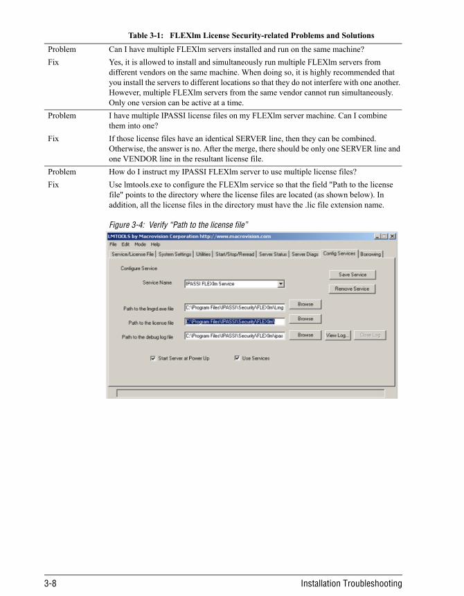
Table 3-1: FLEXlm License Security-related Problems and Solutions

Problem Can I have multiple FLEXlm servers installed and run on the same machine?Fix Yes, it is allowed to install and simultaneously run multiple FLEXlm servers from

different vendors on the same machine. When doing so, it is highly recommended that you install the servers to different locations so that they do not interfere with one another. However, multiple FLEXlm servers from the same vendor cannot run simultaneously. Only one version can be active at a time.

Problem I have multiple IPASSI license files on my FLEXlm server machine. Can I combine them into one?

Fix If those license files have an identical SERVER line, then they can be combined. Otherwise, the answer is no. After the merge, there should be only one SERVER line and one VENDOR line in the resultant license file.

Problem How do I instruct my IPASSI FLEXlm server to use multiple license files?Fix Use lmtools.exe to configure the FLEXlm service so that the field "Path to the license

file" points to the directory where the license files are located (as shown below). In addition, all the license files in the directory must have the .lic file extension name.

Figure 3-4: Verify “Path to the license file”


Problem How can I make FLEXlm security work with firewall on the FLEXlm server machine?Fix To make FLEXlm security work with firewalls, the following three components must be

configured correctly.

1. Use a port number on the SERVER line in the license file as follows: SERVER host hostid [port]

Example: SERVER ips-sol07 0002b303df80 27000

2. Use another port number on the VENDOR line in the license file: VENDOR vendor [port=]port

Example: VENDOR IPASSI port=27001

3. On the application machine, set the value of the environment variable IPASSI_LICENSE_FILE to be 27000@ips-sol07. The port number here is the port number from the SERVER line.

4. Make sure both the ports are enabled on the FLEXlm server machine.5. Ensure that the port numbers for the SERVER line and for the VENDOR line are

not used by other applications on the FLEXlm server machine, and are different from each other.

Problem How do I automatically launch my FLEXlm server when I reboot my FLEXlm server machines?

Fix For FLEXlm servers on Windows NT/2000/XP/2003 machines, this is possible through the "Config Services" tab. On this tab, check the "Use Services" and the "Start Server at Power Up" check boxes and save the server configuration.

Problem How do I prevent my FLEXlm server from being manipulated by users on other machines?

Fix Beginning with FLEXlm 9.x, when you are starting the FLEXlm server, you can specify that users on other machines cannot shut down the FLEXlm server. To do this, go to the Start/Stop/Reread tab, select the service you are about to start, click the "Advanced settings," and check "lmdown will only work from node where lmgrd is running." Then, click "Start Server."Figure 3-5: Configuring through Start/Stop/Reread tab


Problem If I get the message below when launching a SimSci-Esscor application, what could be going wrong?Figure 3-6: Invalid (inconsistent) license key (-8,544)

Fix A common cause of this error is that the FLEXlm dll on the application is of version 7.2, but the FLEXlm server is 9.5. In this case, run the FLEXlm 9.5 Client Retrofit program to update the application and this should resolve the problem.

Problem How do I obtain the system information about the machine, including the host ID?Fix The FLEXlm utility, lmtools.exe System Settings tab, is always the most accurate for

checking the host ID. Note that when issuing a FLEXlm/TOKEN license, SimSci-Esscor uses Ethernet Address or Disk Volume Serial Number to bind the license. If your FLEXlm cannot start correctly, you may want to verify that the Ethernet Address or Disk Volume Serial number in the license file is consistent with that on the machine. In addition, you may check the Computer/Hostname to verify that this value is the same as the second item on the SERVER line in your license file. An example of lmtools System Settings tab display:

Figure 3-7: Getting the machine information from System Settings tab

Problem How do I configure the usage of my license(s)?Fix Use a FLEXlm options file to specify how the license(s) should be used. For detailed

information, please refer to the Options File documentation.Problem How do I include a FLEXlm options file and how would I know if the FLEXlm server is

using the options file?


Diagnosis of USB Security ProblemsWhen encountering licensing problem with the USB security, you can diagnose the problem following the steps described below:

Step 1 - Verify the active type of license security

This step is to ensure that USB is indeed the active license security type. This selection of security type is made in the main initialization file (*.ini) of the application. These files are usually named after the programs they control (Proii.ini, PipePhase.ini, Datacon.ini, etc.) The easiest way to locate these files is to search the application directory for the *.ini that contains the word [wss_Security]. When the ini file is identified, you need to open the file (Notepad will work fine for this) and find the value of the Type statement in the [wss_Security] section. The active security type

Fix If you use "ipassi.opt" for the name of the options file, then simply put this options file in the FLEXlm server folder (where the lmgrd.exe and IPASSI.EXE are). When the next time the IPASSI FLEXlm server starts, it will automatically read and apply the rules in this file. If the options file does not have the default file name or is not located in the FLEXlm server folder, then you'll need to explicitly specify the options file on the VENDOR line in the license file as follows:VENDOR IPASSI options="C:\Program Files\IPASSI\Security\FLEXlm95\ipassi.opt"Note that if there are any spaces in the path or the file name, put double quotes around the fully qualified path as above. When an options file is in use, you should see an entry similar to that shown below in the FLEXlm server log file, ipassi.log:

16:12:11 (IPASSI) Using options file: "C:\Program Files\IPASSI\Security\FLEXlm95\ipassi.opt"

Problem Can I use a regular FLEXlm license file and a TOKEN license file under the same IPASSI FLEXlm server?

Fix Technically, this configuration should work. However, this is not recommended as the logging and reporting functionalities work differently for FLEXlm and for TOKEN security. For clarity, it is highly recommended that FLEXlm and TOKEN be installed on different license server machines.

Problem We're using FLEXlm over a wide-area network. What can we do to improve the FLEXlm licensing performance?

Fix To shorten the initial connection time between the FLEXlm Client and the FLEXlm Server over a wide-area network, you can specify the FLEXlm server port numbers in the FLEXlm license file. In this case, the Client will know exactly what ports on the Server machine to use when trying to connect to the Server.

Problem We're using FLEXlm over a slow wide-area network. What can we do to allow longer FLEXlm Client/Server initial connection time?

Fix You can set the environment variable FLEXLM_TIMEOUT to a larger value on the Client machine. This value sets the timeout period of a FLEXlm-licensed application when attempting to connect to a license server port in the range 27000-27009. Values are in microseconds, within the range 0 through 2147483647. The default setting is 100000 microseconds.


will not have a semi-colon (;) in front of the Type statement. If USB is not the current active security type, you will need to comment out the current active type by placing a semi-colon at the beginning of the line, and uncomment the ;Type=USB line as follows:

[wss_Security]

Type=USB

;Type=FLXLM95

;Type=FLXnet11

;Type=USB

;Type=TOKEN

;Type=TOKENnet

If USB was not previously the active security type and has now been made the active security type, the user should test the application to verify that the change has corrected the problem. If the USB security still does not work, proceed to Step 2 for further diagnosis.

Step 2 - Examine the USB environment on the machine

For the USB security to work, the machine itself must be able to correctly detect the USB key. This step is to determine if this is the case. With the USB key plugged in, go to the Device Manager and open the Universal Serial Bus Controllers to see whether the entry for the USB key is listed correctly as illustrated below:

Figure 3-8: Verify the USB Key


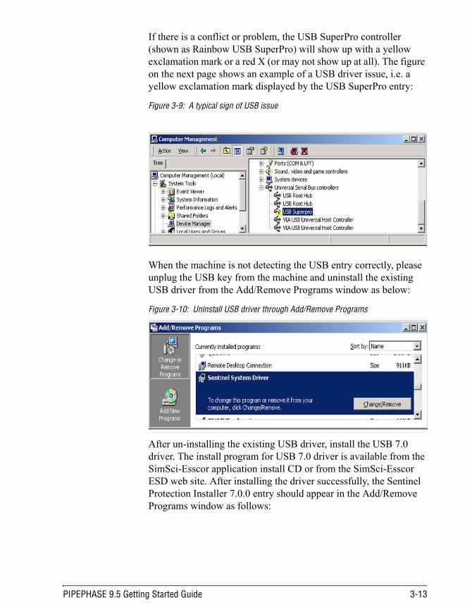
If there is a conflict or problem, the USB SuperPro controller (shown as Rainbow USB SuperPro) will show up with a yellow exclamation mark or a red X (or may not show up at all). The figure on the next page shows an example of a USB driver issue, i.e. a yellow exclamation mark displayed by the USB SuperPro entry:

Figure 3-9: A typical sign of USB issue

When the machine is not detecting the USB entry correctly, please unplug the USB key from the machine and uninstall the existing USB driver from the Add/Remove Programs window as below:

Figure 3-10: Uninstall USB driver through Add/Remove Programs

After un-installing the existing USB driver, install the USB 7.0 driver. The install program for USB 7.0 driver is available from the SimSci-Esscor application install CD or from the SimSci-Esscor ESD web site. After installing the driver successfully, the Sentinel Protection Installer 7.0.0 entry should appear in the Add/Remove Programs window as follows:


Figure 3-11: Verify the upgraded USB driver

Now, plug the USB key back into the machine and go to the Device Manager again to verify that the system is correctly detecting the USB key. If the problem persists, then either the key is damaged or the computer, including the USB port, may be malfunctioning. In this case, the user will either have to try the key on another machine that has a working USB environment to determine if the key is good; or alternatively, the user can try another USB key that is known to be working on another machine to try on the "problem" machine and verify if its USB environment is functioning correctly. If the result indicates that the USB key is not functioning properly, please return the key to SimSci-Esscor technical support for further diagnosis. If the USB environment on the machine is not working correctly, the user will have to resolve the machine problem first.

Another method for examining the USB environment is to use the SuperproMedic utility program (SproMedic.exe) from Rainbow Technology. The install program (SuperproMedic.exe) for this utility is available in the Utility folder in the USB 5.0 Retrofit program, which can be found in the SimSci-Esscor ESD web site. The default install location for this program is C:\Program Files\Rainbow Technologies\SuperPro\Medic. This program displays the version of the current Sentinel System Driver on the machine. Note that not all versions of Sentinel System Driver work with the SimSci-Esscor USB key. If the existing USB driver is not a good one, the SuperproMedic utility program will indicate the problem as shown in the figure below:


Figure 3-12: Version 5.39.2 - Unknown S

In this case, the user will have to unplug the USB key from the machine, un-install the current USB driver, and then re-install the USB 7.0 driver.

When the utility program shows no error in the Sentinel System Driver, the user can click on the Find SuperPro button to see if it can detect the USB key. If it finds the key, the output should look similar to that shown below:

Figure 3-13: 1 Hard limit of first key found

If no keys are detected, the output is as follows (0 Hard limit of first key found):


Figure 3-14: “No SuperPro keys detected”

Step 3 - Examine the SimSci-Esscor USB key and the USB.DLLIf the SproMedic.exe utility can correctly detect the USB key, the next thing to look at is the USB.DLL and the USB key. A potential problem with the USB.DLL is that it may not be recent enough to recognize the applications turned on in the USB key. To eliminate this problem, the user simply downloads the USB 5.0 Retrofit program from the Update area in the SimSci-Esscor ESD web site, and then retrofits the application accordingly to update the USB.DLL. After the retrofitting, the user can run the USBKeyCheck.exe utility program first to see if the USB key is good. If the USBKeycheck.exe program indicates that the USB key has already expired or does not contain the license to run the application, please contact the SimSci-Esscor sales representative to resolve this issue.

Step 4 - Examine the copies of USB.DLL on the machine

Sometimes there are multiple copies of USB.DLL existing on the machine. In this case, the application may or may not be using the newly updated USB.DLL obtained from the previous step. The SimSci-Esscor security files, including USB.DLL, should only exist inside the application folder and the application should only use its own set of security files. Should there be any SimSci-Esscor security files existing outside of all SimSci-Esscor application folders, it is highly recommended that they be deleted to eliminate the confusion, especially those that exist on the paths specified in the PATH environment variable.


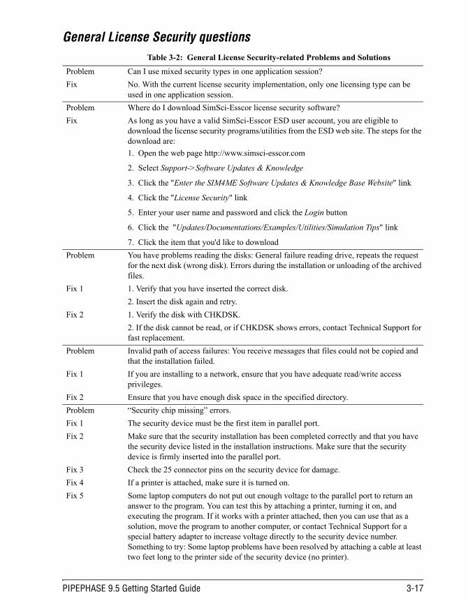
General License Security questionsTable 3-2: General License Security-related Problems and Solutions

Problem Can I use mixed security types in one application session?Fix No. With the current license security implementation, only one licensing type can be

used in one application session.Problem Where do I download SimSci-Esscor license security software?Fix As long as you have a valid SimSci-Esscor ESD user account, you are eligible to

download the license security programs/utilities from the ESD web site. The steps for the download are:1. Open the web page http://www.simsci-esscor.com

2. Select Support->Software Updates & Knowledge

3. Click the "Enter the SIM4ME Software Updates & Knowledge Base Website" link

4. Click the "License Security" link

5. Enter your user name and password and click the Login button

6. Click the "Updates/Documentations/Examples/Utilities/Simulation Tips" link

7. Click the item that you'd like to downloadProblem You have problems reading the disks: General failure reading drive, repeats the request

for the next disk (wrong disk). Errors during the installation or unloading of the archived files.

Fix 1 1. Verify that you have inserted the correct disk.2. Insert the disk again and retry.

Fix 2 1. Verify the disk with CHKDSK.2. If the disk cannot be read, or if CHKDSK shows errors, contact Technical Support for fast replacement.

Problem Invalid path of access failures: You receive messages that files could not be copied and that the installation failed.

Fix 1 If you are installing to a network, ensure that you have adequate read/write access privileges.

Fix 2 Ensure that you have enough disk space in the specified directory.Problem “Security chip missing” errors.Fix 1 The security device must be the first item in parallel port.Fix 2 Make sure that the security installation has been completed correctly and that you have

the security device listed in the installation instructions. Make sure that the security device is firmly inserted into the parallel port.

Fix 3 Check the 25 connector pins on the security device for damage.Fix 4 If a printer is attached, make sure it is turned on.Fix 5 Some laptop computers do not put out enough voltage to the parallel port to return an

answer to the program. You can test this by attaching a printer, turning it on, and executing the program. If it works with a printer attached, then you can use that as a solution, move the program to another computer, or contact Technical Support for a special battery adapter to increase voltage directly to the security device number. Something to try: Some laptop problems have been resolved by attaching a cable at least two feet long to the printer side of the security device (no printer).


Fix 6 Make sure only similar security devices are “piggybacked.”Problem INPLANT is installed on a system running Windows NT. When you run INPLANT, it

produces errors relating to security.Fix Ensure that whoever installed INPLANT had system administration rights/privileges.


Chapter 4Getting Started

Starting PIPEPHASE SoftwareIf you do not see a PIPEPHASE 9.5 icon in a SIMSCI group window or in your Program Manager window, see the troubleshooting section in the PIPEPHASE Installation Guide.

To start PIPEPHASE software:

➤ Double-click on the PIPEPHASE 9.5 icon.

The main PIPEPHASE window appears.

Figure 4-1: The PIPEPHASE Main Window


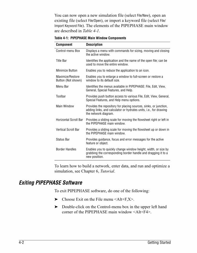
You can now open a new simulation file (select File/New), open an existing file (select File/Open), or import a keyword file (select File/Import Keyword File). The elements of the PIPEPHASE main window are described in Table 4-1.

To learn how to build a network, enter data, and run and optimize a simulation, see Chapter 6, Tutorial.

Exiting PIPEPHASE SoftwareTo exit PIPEPHASE software, do one of the following:

➤ Choose Exit on the File menu <Alt+F,X>.

➤ Double-click on the Control-menu box in the upper left hand corner of the PIPEPHASE main window <Alt+F4>.

Table 4-1: PIPEPHASE Main Window Components

Component Description

Control-menu Box Displays a menu with commands for sizing, moving and closing the active window.

Title Bar Identifies the application and the name of the open file; can be used to move the entire window.

Minimize Button Enables you to reduce the application to an icon.

Maximize/Restore Button (Not shown)

Enables you to enlarge a window to full-screen or restore a window to its default size.

Menu Bar Identifies the menus available in PIPEPHASE: File, Edit, View, General, Special Features, and Help.

Toolbar Provides push button access to various File, Edit, View, General, Special Features, and Help menu options.

Main Window Provides the repository for placing sources, sinks, or junction, adding links, and calculator or hydrates units, i.e., for drawing the network diagram.

Horizontal Scroll Bar Provides a sliding scale for moving the flowsheet right or left in the PIPEPHASE main window.

Vertical Scroll Bar Provides a sliding scale for moving the flowsheet up or down in the PIPEPHASE main window.

Status Bar Provides guidance, focus and error messages for the active feature or object.

Border Handles Enables you to quickly change window height, width, or size by grabbing the corresponding border handle and dragging it to a new position.

4-2 Getting Started

Manipulating the PIPEPHASE Window The PIPEPHASE window offers a variety of features that enable you to customize how PIPEPHASE software appears relative to the full screen and relative to other applications.

Changing Window Size The Windows interface provides tools for resizing each window. Some tools automatically change a window to a particular size and orientation, others enable you to control the magnification.

To display the control-menu box:

➤ Click on the control-menu box in the top left hand corner of the PIPEPHASE main window or use <Alt+Space>.

➤ Select the Move option from the menu.

Working with On-screen Color Coding Cues PIPEPHASE software provides the standard visual cue (grayed out text and icons) for unavailable menu items and toolbar buttons. In addition, on the network, PIPEPHASE software uses colored borders liberally to indicate the current status of the simulation.

Note: PIPEPHASE software does not support multiple sessions for two different files located in the same directory.

Tools Description/Action

Minimize/Maximize Buttons

By clicking on the minimize and maximize buttons, you can automatically adjust the size of a window.

Border Handles You can use the window border to manually change the size of the main window. The border works like a handle that you can grab with the cursor and drag to a new position.

Control Menu You can also use the Control menu to Restore, Move, Size, Minimize, or Maximize a window.

Window Position You can change the position of the main window (or any pop-up window) by clicking on the title bar and dragging the window to a new position.

Control-menu Box You can also use the control-menu box to move a window.

Table 4-2: Flowsheet Color Codes

Color Significance

Red Required data. Actions or data required of the user. On the main PIPEPHASE windows and Link PFD only.

Blue Data you have supplied.


Using the Menus The names of the PIPEPHASE main menus appear on the menu bar. From these menus, you can access most PIPEPHASE operations.

To display a menu:

➤ Click on the menu name or press <Alt+n> where n is the underlined letter in the menu name.

For example, to display the File menu, either click on File, or press <Alt+F>.

Burgundy Calculated data.

Gray Data field not available to you.

Table 4-2: Flowsheet Color Codes

Color Significance

Figure 4-2: File Menu Figure 4-3: Edit Menu

Figure 4-4: View Output Menu Figure 4-5: General Menu

4-4 Getting Started

Choosing a Menu Item To choose a menu item, do one of the following:

➤ Click on the desired item.

➤ Use the arrow keys to highlight the item, then press <Enter>.

➤ Use the accelerator keys.

Using the Toolbar Buttons

Figure 4-8: Toolbar Buttons

The toolbar contains four groups of buttons:

➤ File Manipulation Buttons

➤ Structure and Unit Operation Buttons

➤ Calculation Options, Optimization, and Property Buttons

➤ Zoom and Redraw Buttons

Figure 4-6: Special Features Menu

2

Figure 4-7: Help Menu

Note: Grayed out icons indicate that the functions are currently in passive mode and will become active when necessary.


Using the File Manipulation Buttons These buttons enable you to open a new or existing simulation, import a keyword file, save a simulation, run a simulation, or view or print an output. These buttons duplicate menu options available on the File menu.

Using the Structure and Unit Operation Buttons These buttons enable you to add sources, sinks, junction, calculator units, or hydrate units to the flowsheet.

Button Menu Item Description

New Enables you to create a new simulation

Open Enables you to open an existing simulation

Import Keyword File Enables you to import an existing input file

Save Enables you to save an open simulation

Run Enables you to run the simulation

Excel Reports Enables you to create Excel® Reports

Sim4Me Enables you to open Sim4Me Portal

Note: PIPEPHASE software permits the users to save, import and open files from locations with file path length of up to 120 characters and file name length of up to 64 characters.


— Enables you to add a source to the flowsheet

— Enables you to add a sink to the flowsheet

— Enables you to add a junction to the flowsheet

— Enables you to add a Manifold unit to the flowsheet

— Enables you to add a calculator unit to the flowsheet

— Enables you to add a hydrate unit to the flowsheet

4-6 Getting Started

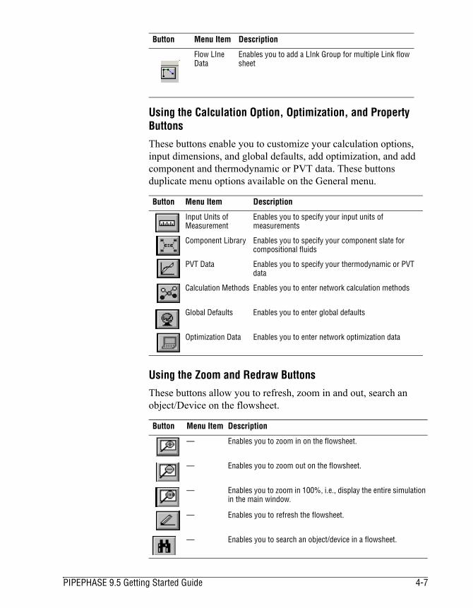
Using the Calculation Option, Optimization, and Property Buttons These buttons enable you to customize your calculation options, input dimensions, and global defaults, add optimization, and add component and thermodynamic or PVT data. These buttons duplicate menu options available on the General menu.

Using the Zoom and Redraw Buttons These buttons allow you to refresh, zoom in and out, search an object/Device on the flowsheet.

Flow LIne Data

Enables you to add a LInk Group for multiple Link flow sheet


Input Units of Measurement

Enables you to specify your input units of measurements

Component Library Enables you to specify your component slate for compositional fluids

PVT Data Enables you to specify your thermodynamic or PVT data

Calculation Methods Enables you to enter network calculation methods

Global Defaults Enables you to enter global defaults

Optimization Data Enables you to enter network optimization data


— Enables you to zoom in on the flowsheet.

— Enables you to zoom out on the flowsheet.

— Enables you to zoom in 100%, i.e., display the entire simulation in the main window.

— Enables you to refresh the flowsheet.

— Enables you to search an object/device in a flowsheet.



Using PIPEPHASE Software

Defining the ApplicationThis section contains information about the way PIPEPHASE software works, the data that you need to supply, and the correlations used.

This section is arranged according to what you want to do, the type of fluid you have, and the type of pipeline network. For each of the capabilities of PIPEPHASE software, this chapter explains which data you are required to provide and which data you may optionally supply. Throughout this section, the right hand column (See...) provides the title of the GUI window where you can input that data, or the manual where additional information can be found.

The first thing you should do before using PIPEPHASE is to decide what type of application you have. This depends on:

■ The properties of the fluid(s) flowing through the piping sys-tem,

■ The flowrates and conditions at which those fluids enter and leave the piping system,

■ The structure and elements of the piping system, and

■ Other special processes you want to simulate, such as Gas Lift Analysis.

Properties of Fluids

There are seven types of fluids modeled in PIPEPHASE software:

■ Compositional

● Mixed phases

● Liquid

● Vapor

■ Compositional Blackoil

■ Non-compositional

● Blackoil

● Gas Condensate

4-8 Getting Started

● Gas

● Liquid

● Steam

The fluid type controls how the program is able to obtain the physical properties necessary for pressure drop and heat transfer calculations – either from the PIPEPHASE databank, from built-in empirical correlations, or from user-supplied input. Steam is a special case of a non-compositional fluid, for which PIPEPHASE software uses the GPSA steam tables.

Compositional fluids are defined as mixtures of chemical components with a known composition. For compositional fluids, PIPEPHASE software will calculate the phase separation whenever prevailing process fluid conditions are required. However, you may instruct PIPEPHASE software to assume the fluid is one phase at all times, thus reducing the time the program takes to solve by continually bypassing the vapor-liquid equilibrium (flash) calculation.

Non-compositional gases and liquids are single-phase. Blackoil is a liquid-dominated, two-phase model. Gas Condensate is a gas-dominated, two-phase model. Steam is a single component, two-phase model.

Optimization

PIPEPHASE software can optimize network problems of virtually any size. You can minimize or maximize any objective function or even tune your simulation to match measured data, while satisfying operational or design constraints. A PIPEPHASE model can be optimized over time resulting in efficient optimized design, planning, forecasting, and operation of a field.

Link to Reservoir Simulator Models

PIPEPHASE software’s Reservoir Interface allows you to link the network simulator to Reservoir Simulation models such as the GEMS reservoir simulation model. This integrated solution provides greater simulation consistency and accuracy, resulting in savings of millions of dollars over the lifetime of a field in terms of planning and scheduling.

Flows and Conditions of Fluids


Fluids enter piping systems at sources and leave at sinks. Fluids with different properties may enter at different sources, but they must all be of the same type.

In general, you have to assign flowrates, temperatures and pressures to sources and/or sinks. For compositional fluids, you also have to assign compositions to the source fluids. The exceptions are explained below in What PIPEPHASE Calculates.

Gaslift and Sphering

Two special applications, relevant to oil production and gas transportation, can be modeled with PIPEPHASE software. You can use PIPEPHASE software to investigate the effects of lift gas on well production and optimize the allocation of limited lift gas for multiple wells. Sphering or Pigging is used to increase gas flow efficiency in wet gas and gas dominated multiphase pipelines.

Piping Structure

Before providing input problem data to PIPEPHASE software, it is important that you convert the structure of the piping system into a simpler schematic representation of the relevant nodes (i.e., sources, junctions, and sinks) and links. You must label each node and link both uniquely and logically for future reference.

What PIPEPHASE Software Calculates

PIPEPHASE software solves the equations that define the relationship between pressure drop and flowrate. PIPEPHASE software can also calculate heat losses and gains.

With a single link, PIPEPHASE software will calculate the pressure drop for a known flowrate. Alternatively, for a given pressure drop, PIPEPHASE software will calculate the flowrate.

With a network configuration, you may supply a combination of known flowrates and pressures at sources and/or sinks and PIPEPHASE software will calculate the unknowns. The combination of knowns that you are allowed to supply are explained later on.

Rating, Design, Case Studies, and Nodal Analysis

PIPEPHASE software works in both rating and design modes. In rating mode, you supply data about the pipes, fittings and equipment and PIPEPHASE software calculates the pressure and

4-10 Getting Started

temperature profiles. In design mode, PIPEPHASE software calculates line sizes. Case Studies can be performed in either mode. Nodal Analyses can be performed on single links.

Global SettingsBefore you provide PIPEPHASE software with information about the fluid and piping structure of your problem, global parameters may be set and the problem definition described. Choices can be made on control of the simulation, define the input units, specify how much output you want, and set global defaults for use throughout the simulation.

Units of Measurement

PIPEPHASE software allows you to construct a group of units of measure (or “dimensions”) which are to be used throughout the entire simulation input. However, you can locally override individual units of measure where necessary. The output will

To provide... See...

Descriptive text You can further describe the problem using up to four lines of 60 characters each. This description appears once at the top of each page.

Simulation Description

If you are using the Case Study facility, you may add one line of description for each case study. You will find further details about case studies later in this chapter.


If you are using the Nodal Analysis facility, you may add two lines of description, one for inflow and one for outflow. You will find further details about nodal analysis later in this chapter.


Input data checking

You may use PIPEPHASE software just to check your input syntax and topology and not to perform any calculations.

Run Simulation and View Results


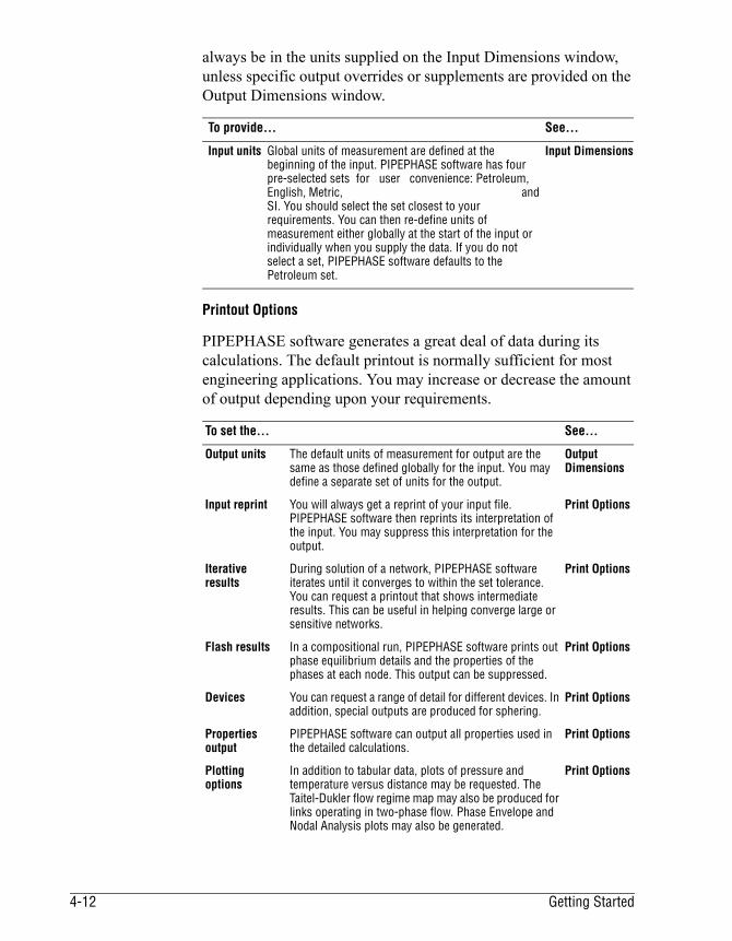
always be in the units supplied on the Input Dimensions window, unless specific output overrides or supplements are provided on the Output Dimensions window.

Printout Options

PIPEPHASE software generates a great deal of data during its calculations. The default printout is normally sufficient for most engineering applications. You may increase or decrease the amount of output depending upon your requirements.

To provide... See...

Input units Global units of measurement are defined at the beginning of the input. PIPEPHASE software has four pre-selected sets for user convenience: Petroleum, English, Metric, and SI. You should select the set closest to your requirements. You can then re-define units of measurement either globally at the start of the input or individually when you supply the data. If you do not select a set, PIPEPHASE software defaults to the Petroleum set.

Input Dimensions

To set the... See...

Output units The default units of measurement for output are the same as those defined globally for the input. You may define a separate set of units for the output.

Output Dimensions

Input reprint You will always get a reprint of your input file. PIPEPHASE software then reprints its interpretation of the input. You may suppress this interpretation for the output.

Print Options

Iterative results

During solution of a network, PIPEPHASE software iterates until it converges to within the set tolerance. You can request a printout that shows intermediate results. This can be useful in helping converge large or sensitive networks.

Print Options

Flash results In a compositional run, PIPEPHASE software prints out phase equilibrium details and the properties of the phases at each node. This output can be suppressed.

Print Options

Devices You can request a range of detail for different devices. In addition, special outputs are produced for sphering.

Print Options

Properties output

PIPEPHASE software can output all properties used in the detailed calculations.

Print Options

Plotting options

In addition to tabular data, plots of pressure and temperature versus distance may be requested. The Taitel-Dukler flow regime map may also be produced for links operating in two-phase flow. Phase Envelope and Nodal Analysis plots may also be generated.

Print Options


Defaults

Many of PIPEPHASE software’s data items are defaulted. If you do not explicitly specify an item or a calculation method, the program will automatically assign a value or method. These values – for example 29 BTU/hr-ft-oF for pipe thermal conductivity and the Moody method for single-phase pressure drop calculations – have been selected to be reasonable for normal engineering purposes, but are not necessarily the best for your particular application. They are there for your convenience and are not intended to replace engineering judgement. You should check that you do not get invalid results through their use.

For convenience, PIPEPHASE software allows you to change some defaults globally at the start of the input.

Results Access System (RAS)

Using the PIPEPHASE RAS, you may examine data that have been produced by a run of the program. You may also print or plot the results using Excel spreadsheet.

PIPEPHASE RAS Main Window

Optimizer Output

You can set the printout level of optimizer cycle results and control the output of the intermediate results.

Print Options

To define... See...

Flow device parameters

You can specify global values for the pipe, riser, tubing and annulus inside diameter, the surrounding medium, and the parameters associated with pressure drop and heat transfer. You can override these settings for individual pipes.

Global Defaults

Heat Transfer You can define the heat transfer from pipes, risers, tubings, and annuli as an overall coefficient or by defining the parameters - viscosity, conductivity, velocity, etc. - for the surrounding soil, air, or water. You can select a medium and optionally override these settings for individual pipes. You can globally suppress heat transfer calculations and then reinstate them for individual pipes, risers, tubings, and annuli.

Global Defaults

Pressure drop methods

You can globally set the pressure drop method and the Palmer parameters for liquid holdup. You can override the pressure drop method for individual pipes, risers, tubings, and annuli.

Global Defaults

Transitional flow

You can globally set the transitional Reynolds Number between laminar and turbulent flow regimes.

Global Defaults

Limits You can change the maximum and minimum values of temperature and pressure for flash calculations. If the program detects conditions outside these limits, warning messages will be presented in the output.

Global Defaults

To set the... See...


Defining Fluid PropertiesPIPEPHASE software requires the properties of the fluid to calculate pressure drops, heat transfer and phase ratios. There are two major classifications of fluid models: compositional and non-compositional.

A fluid model is compositional when it can be defined in terms of its individual components either directly or through an assay curve. PIPEPHASE software will then predict the fluid’s properties by applying the appropriate mixing rules to the pure component properties. Unless PIPEPHASE software is instructed otherwise, it will perform phase equilibrium calculations for the fluid and determine the quantity and properties of the liquid and vapor phases.

A fluid model is non-compositional when it is defined with average correlated properties.

Defining Properties for Compositional FluidsPIPEPHASE software requires thermodynamic and transport properties to calculate phase splits, pressure drops, and heat transfer.

All required properties of compositional fluids are predicted from the properties of the pure components. These are mixed to get the properties of the fluid.

There are three methods for defining a component:

➤ Selecting individual components from the PIPEPHASE library,

➤ Defining individual components as petroleum pseudocomponents,

➤ Defining an assay curve and having PIPEPHASE software divide it into petroleum cuts.

The compositional fluid can be defined in terms of any combination of these options. You can have different compositions at each source.

Water as a Special Component

PIPEPHASE software can rigorously predict phase separations involving more than one liquid phase. However, there is a simplified way of dealing with water in hydrocarbon systems.


Because water is only sparingly soluble in oil, a hydrocarbon system with a significant amount of water will often form two liquid phases. PIPEPHASE software will handle calculations involving water in hydrocarbons by one of three methods:

➤ Rigorous three-phase flash to calculate composition in three phases.

➤ It can calculate the solubility of water in the hydrocarbon phase and put the excess water into a pure aqueous phase. All the aqueous phase properties will be calculated separately from those of the hydrocarbon phase.

➤ It can assume that the water is completely soluble.

Library Components

The SIMSCI library contains over 1700 components. A full list is available in the SIMSCI Component and Thermodynamic Data Input Manual. For all components, the databank contains data for all the fixed properties and temperature-dependent properties necessary to carry out phase equilibrium calculations. For all common components, the databank also contains a full set of transport properties necessary to carry out pressure drop and heat transfer calculations. If you need to supplement the data, or override the library data with your own, you may do so.

Non-library Components

You may use components not found in the SIMSCI library. You must input all the necessary data for thermodynamic and transport properties. If you need help in determining data for such components, you may use SIMSCI’s DATAPREP program.

Petroleum Pseudocomponents

To specify... See...

Library components

All fixed property data may be accessed from the SIMSCI databank. All you need to do is supply the name of the component.

➱ Component Data, Library Component Data

You may override the SIMSCI constant properties for any or all of the components.

➱ Component Data, Edit Library Component

You may override the SIMSCI variable (temperature-dependent) properties for any or all of the components.

SIMSCI Component and Thermodynamic Data Input Manual

Non-library components

If you want to use a component that is not in the SIMSCI Bank, you must supply its name and all the required properties.

➱ SIMSCI Component and Thermodynamic Data Input Manual


To define hydrocarbon pseudocomponents, you must supply at least two of the following three parameters:

➤ Molecular weight

➤ Gravity

➤ Normal boiling point

PIPEPHASE software will predict the third if you omit it. PIPEPHASE software uses industry-standard characterization methods to predict all fixed and temperature-dependent property data for each pseudocomponent. You may select the method most suitable for your own mixture.

Assay Curve

If your fluid is defined by an assay curve (TBP, D86, D2887, or D1160), PIPEPHASE software will divide it into a number of cuts. You can control the number of cuts and the ranges they cover. Each of the cuts is then treated as a pseudocomponent, as described previously. You may also define a lightends analysis to go with the assay curve.

To supply ... See...

Pseudocomponents

Define petroleum pseudocomponents by supplying at least two of the following: molecular weight, gravity, and normal boiling point.

➱ Component Data, Library Component Data

Property calculation methods

You may select the method PIPEPHASE software will use to calculate the properties of your pseudocomponents.

➱ Component Data

Fixed Property Data

You can supply your own fixed property data to override the data that PIPEPHASE software predicts.

➱ Component Data

Variable Property Data

You can supply your own temperature-dependent property data to override the data that PIPEPHASE software predicts.

➱ Component Data


Assay Data You supply an assay curve, and PIPEPHASE software will divide it into petroleum cuts. You supply it in the form of D86, D1160, D2887, TBP, or TBP at 10 mm Hg curves.

➱ Component Data

You must also supply gravity as API or specific gravity or UOP K-factor either as a curve against percent vaporized or as an average value.

➱ Component Data


Additional Component Capabilities

All the features of SIMSCI’s industry-standard component property databank and methods have been incorporated into PIPEPHASE software. These are summarized in Table 4-3. For details of these methods and their applicability, please consult the SIMSCI Component and Thermodynamic Data Input Manual, in the chapter detailed below.

Thermodynamic Properties and Phase Separation

PIPEPHASE software can use a generalized correlation, an equation of state, or a liquid activity method to calculate thermodynamic properties at the flowing conditions and hence predict the split between the liquid and vapor phases. The choice of the thermodynamic property calculation method depends on the components in the fluid and the prevailing temperatures and

PIPEPHASE software will calculate molecular weight data, or you may supply it as an average or a curve against percent vaporized.

➱ Component Data

You may define the number of petroleum fractions to be generated and their temperature ranges.

➱ Component Data, Temperature Cut Points

You may select the method PIPEPHASE software will use to calculate the properties of the generated petroleum fractions.

➱ Component Data

Mixed component types

You can mix defined components and pseudocomponents with assay data by defining a lightends composition and rate for each source.

➱ Component Data

Table 4-3: Summary of Other Component Property Options

Synthetic Components

You may characterize a component as a synfuel of a specific type or as a mixture of different petroleum types.

Chapter 1

Other fixed property requirements

Rackett parameter is required for the Rackett method for liquid densities.Dipole moment and Radius of gyration are required for the Hayden-O’Connell method for vapor properties.Hildebrand solubility parameter and liquid molar volume are required for various generalized and liquid activity thermodynamic correlations. Van der Waal’s area and volume are required for UNIFAC and UNIQUAC liquid activity thermodynamic correlations.

Chapter 1

Properties from Structure

You may define the structure of non-library components for use with the UNIFAC thermodynamic method.

Chapter 1



pressures. PIPEPHASE software also provides a number of methods that can rigorously calculate vapor-liquid-liquid equilibrium.

Table 4-4 gives recommendations for the commonly found pipeline systems.

Table 4-4: Recommended Methods for Thermodynamic Properties

Method

Property Heavy Hydrocarbon Systems

Light HydrocarbonSystems

Natural GasSystems

K-value Braun K10 (<100 psia)Grayson-StreedPeng-RobinsonSoave-Redlich-Kwong

Peng-RobinsonSoave-Redlich-KwongLee-Kesler-PlöckerBenedict-Webb-Rubin-Starling Chao-Seader

Peng-RobinsonSoave-Redlich-Kwong

Enthalpy Curl-PitzerJohnson-GraysonLee-KeslerPeng-RobinsonSoave-Redlich-Kwong

Peng-RobinsonSoave-Redlich-KwongLee-Kesler-PlöckerBWRSCurl-PitzerLee- Kesler


Liquid Density

APILee-Kesler

APILee-Kesler

APILee-Kesler

Vapor Density





K-values, enthalpy, density

You must select a thermodynamic method for calculating the vapor-liquid equilibrium and mixture properties from component properties. Either select a system with a predefined method for each property, or select an individual method for each property.

➱ Thermodynamic Methods

Vapor-liquid-liquid equilibria

You can specify a VLLE thermodynamic system or K-value method or specify a second LLE K-value method.


Different enthalpy methods for liquid and vapor

You must include two enthalpy methods, one for the liquid and one for the vapor.


Different density methods for liquid and vapor

You must include two density methods, one for the liquid and one for the vapor.


Aqueous phase enthalpy

If you have water in a hydrocarbon system, you may select a method for calculating aqueous liquid and vapor enthalpies either by a simplified method which assumes that the steam is at its saturation point or by a rigorous method which takes into account the degree of superheat of the vapor, if any.



Transport Properties

The SIMSCI databank contains pure component data for the thermal conductivity, surface tension, and viscosity of liquids and vapors as functions of temperature. You can choose to use these data and simple mixing rules to predict the flowing properties of the fluid.

Alternatively you can choose to use the API Data Book property prediction methods and mixing rules for mixed hydrocarbons.

Some 60 of the bank components have data for viscosity and thermal conductivity from the GPA TRAPP program. If you choose to use the TRAPP data, all of your components must be TRAPP components and you cannot have any pseudocomponents or assay data.

Using Multiple Methods

In most cases, a single set of thermodynamic and transport methods is adequate for calculating properties of all sources. However, your flowsheet may contain sources with widely varying compositions or

Binary interaction parameters

For some systems, notably close-boiling mixtures, the standard equations do not adequately reproduce experimental phase equilibria data. You may improve the predictability of many of the equations of state, or liquid activity coefficient methods by inputting your own binary interaction parameter values. For example, you can tune the PR, SRK, BWRS and LKP equations.



Prediction methods

You may choose a method for calculating bulk transport properties from component properties. Select a system with predefined methods for each property, or select an individual method for each property.


Overriding viscosity

To override the mixture liquid viscosity predictions, you may supply a liquid viscosity curve for either the hydrocarbon liquid phase, the water phase or the total liquid. A different viscosity curve may be supplied for each source.

➱ Thermodynamic Methods, User Viscosity Data



conditions such that they cannot be simulated accurately using just one set. For this, you may define more than one set of methods (there is no limit) and apply different sets to different sources.

Additional Thermodynamic Capabilities

All of SIMSCI’s industry-standard thermophysical property calculation methods have been incorporated into PIPEPHASE software. These are summarized in Table 4-5. For details of these methods and their applicability, please consult Chapter 2 in the SIMSCI Component and Thermodynamic Data Input Manual.


More than one thermodynamic set

For each set use a separate METHOD statement. Name the set using the SET keyword.

➱ Fluid Property Data, Thermodynamic Methods

The set used by a source

Link the source to the thermodynamic set using the SET keyword.

➱ Compositional Source

A default thermodynamic set

When a single set is present, all sources use that set. If you do not link the source to a thermodynamic set, it will use the default set. Normally this is the first set that appears in the input. You can stipulate that another set is the default, by setting that set as the default.


Table 4-5: Summary of Other Thermodynamic Options

Generalized Correlations

Grayson-StreedImproved-Grayson-StreedGrayson-Streed-ErbarBraun-K10

Chao-SeaderChao-Seader-ErbarIdeal

Equations of State

Soave-Redlich-KwongSRK-Kabadi-DannerSRK-Huron-VidalSRK-Panagiotopoulos-ReidSRK-ModifiedSRK-SIMSCISRK-Hexamer

Panagiotopoulos-ReidPeng-RobinsonPR-Huron-VidalPR-Panagiotopoulos-ReidBWRSUniwaals


Defining Properties for Non-compositional FluidsA non-compositional fluid model must be defined as blackoil, gas condensate, liquid, gas, or steam. Blackoil and gas condensate are two-phase, with one phase dominant. Gas and liquid fluid models are single-phase. Steam may be single- or two-phase.

Liquid

All properties of a non-compositional liquid are calculated by PIPEPHASE software from the specific gravity and built-in correlations.

Liquid Activity Methods

Non-random Two-liquid EquationUniversal Quasi-chemical (UNIQUAC)van LaarWilsonMargulesRegular Solution TheoryFlory-Huggins Theory

Universal Functional Activity Coefficient (UNIFAC)Lyngby-modified UNIFACDortmund-modified UNIFACModified UNIFAC methodFree volume modification to UNIFACIdeal

Special Packages

GlycolSourGPA Sour Water

AmineAlcohol

Other Features

Heat of MixingPoynting Correction

Henry’s LawAmine Residence TimeCorrection

To... See...

Define the fluid You must tell PIPEPHASE software the type of fluid you have; blackoil, gas condensate, liquid, gas, or steam.

➱ Simulation Definition

Supply different data for different sources

You may supply specific gravities for each source.

➱ Source

To... See...

Define the liquid You must define the liquid as water or hydrocarbon, and supply its gravity. If the liquid is water, the specific gravity must be 1.0 or greater. For liquid hydrocarbon, the specific gravity must be less than 1.0.

➱ Single Phase Liquid PVT Data

Specify the viscosity method

You may define the method that PIPEPHASE software uses to predict non-compositional liquid viscosity.


Table 4-5: Summary of Other Thermodynamic Options


Gas

All properties of a non-compositional gas are calculated by PIPEPHASE software from the specific gravity and the built-in correlations.

Steam

Override viscosity data

You may supply liquid viscosity data to override the internally predicted data. You may define the viscosity as a single value or as a two-point viscosity curve.


Specify the specific heat

You may supply a single constant value for liquid specific heat to override the internally predicted data.


To... See...

Define the gas A non-compositional gas is defined in terms of its gravity, and PIPEPHASE software will use the appropriate correlations to predict its properties.

➱ Single Phase Gas PVT Data


You may define the method that PIPEPHASE software uses to predict non-compositional gas viscosity.


Define the Cp/Cv ratio

A gas specific heat ratio may be defined to override the internal value used as default.


Define a contaminant

One or more of the following gas contaminants may also be defined: nitrogen, carbon dioxide, or hydrogen sulfide.


Supply the gasZ-factor

The method that PIPEPHASE software uses to predict a non-compositional compressibility factor may also be defined.


To... See...


Steam is a non-compositional fluid that is allowed to exist in two phases. You cannot override the steam table data contained within PIPEPHASE software’s data libraries. However, all pressure drop correlations which are available to compositional fluids are also available to the steam model.

Gas Condensate

Gas condensate is a multiphase non-compositional fluid with gas predominating. All properties of gas condensate are calculated by PIPEPHASE software from the specific gravity and the built-in correlations.

Blackoil

Blackoil is a multiphase fluid model which predicts properties from the gas gravity, oil gravity, and the standard volume of gas per standard unit volume of oil.

To... See...

Use the steam tables

If the fluid is steam, use PIPEPHASE software ‘s internal steam tables. You may specify that the gravity of the condensed water is more than 1.0 to take into account dissolved solids.

➱ Stream PVT Data

Specify saturated steam

You may specify steam quality if the steam is saturated. Specify the temperature and quality if the steam is superheated or the water is subcooled.

➱ Source

To... See...

Define the condensate

A gas condensate is defined in terms of its gravity, and PIPEPHASE software will use the appropriate correlations to predict its properties.

➱ Gas Condensate PVT Data

Define the specific gravity

You must supply specific gravity data for gas, liquid and water phases, even if you do not expect them all to be present.





To... See...

Define the Blackoil

Blackoil is defined in terms of the gravity of its oil and gas and the Gas to Oil ratio. PIPEPHASE software will use the appropriate correlations to predict its properties.

➱Blackoil PVT Data

Define the specific gravity

You must supply specific gravity data for gas, liquid, and water phases, even if you do not expect them all to be present.


Define the viscosity

You may optionally enter liquid viscosity data in the form of a two-point Antoine curve.



Defining Properties for Mixed Compositional/Non-Compositional FluidsPIPEPHASE software offers the user the ability to define blackoil models that combine data from:

■ sources that are in the standard black oil format (see description of blackoil inputs),

with

■ sources that are in the standard compositional format (see description of compositional inputs).

PIPEPHASE software treats the combined fluid model as a blackoil model; flash calculations are used to define the appropriate blackoil properties for the compositional sources. The inputs to the compositional blackoil model are thus a combination of the inputs to separate compositional and blackoil models.




Adjust properties You may adjust the properties that PIPEPHASE software calculates from its built-in correlations so that they more closely fit measured laboratory data.


Define Lift Gas When you have a GLVALVE in the simulation, you need to define the lift gas in terms of Gravity and (optionally) contaminants.

➱Blackoil Liftgas Data

Tabular Data If laboratory data are available, you may input them and override the PIPEPHASE software internally generated data. If you use tabular data, you must input all data: Formation Volume Factor, Solution Gas Oil Ratio, Live Viscosity, and Gravity.


Supply the gas Z-factor

The method that PIPEPHASE software uses to predict a non-compositional compressibility factor may be defined.

➱Blackoil PVT Correlations Data


You may define the method that PIPEPHASE software uses to predict viscosities and blending rules.


Specify formation volume factor and solution gas oil ratio methods

You may define the methods that PIPEPHASE software uses to calculate formation volume factor and solution gas oil ratio.


To... See...


Generating and Using Tables of PropertiesFor large scale compositional or blackoil simulations, a table of fluid properties can be built and used. This will reduce the computation time by phase separation calculations during the solution procedure. This method is applicable if all the sources in the network have the same composition or Blackoil properties.

SourcesA source is a point at which fluid enters the piping system. You define a source by supplying parameters such as composition, temperature, pressure, and flowrate. You can have more than one source in a network.

Compositional Sources

To... See...

Build and use a table

You can have PIPEPHASE software build the table and use it in the same run.

➱ Generate PVT Table

Retrieve a table

Alternatively, you can have PIPEPHASE software build the table, store it in a file, and then use it in a subsequent run. PIPEPHASE software will not build a table for use in the same run while also storing it for a subsequent run.

➱ Fluid Property Data


Defined components

You must define the total flowrate and composition of the source stream. Components can be either from the PIPEPHASE component library or defined as pseudocomponents.

➱Compositional Source

Assay data A source fluid may be defined by an assay curve. You can combine library components and/or petroleum pseudocomponents with an assay curve by supplying a lightend analysis.


Viscosity data

To override the internally generated fluid viscosity data, you may specify a viscosity curve in the PVT data section.


Similar sources

To reduce redundant data entry, you may refer to a predefined source. Parameters may be specified to override the parameters that are different.



Non-compositional Sources

Structure of Network SystemsFlow devices such as pipes, risers, fittings, and other process equipment are connected together in a Link. Each Link starts at a Node (a Source or a Junction) and ends at another Node (a Junction or a Sink).

PIPEPHASE software can calculate either single link or network problems. A single link is defined as a series of pipes, fittings, and process equipment that has one source, one sink, and no junctions. A network may have one or more sources and one or more sinks.

PIPEPHASE software calculates the flowrates and pressure drops. In a network configuration, you must either define these parameters or provide an estimate at each node.


Steam sources

You must define the pressure and quality of a saturated steam source. The temperature must be specified only if the steam is superheated (Quality=100%) or subcooled (Quality=0%).

➱Steam Source

Gas, liquid, blackoil or condensate sources

One or more sets of fluid property data are defined in the PVT data section. You must assign a unique set number to each data set. Each source must be referred to the appropriate data set number.

➱Blackoil Source

Well In-flow Performance

You may specify the IPR of a well source for a single link with gas, liquid, blackoil or condensate. The IPR Model is treated as a device and is available from the Link window. You may also supply well test data.

➱Link Device Data, Inflow Performance Relationship, IPR-Advanced Options

Similar sources

If one source is the same as or similar to another, you may refer it to the other source. PIPEPHASE software will copy all the data from one source to the other. You may then override the parameters that are different.

➱Reference Source


Network solution algorithm

There are two solution algorithms available for Networks. For the vast majority of networks, you would use the default PBAL method. If your fluid is a single-phase liquid or gas, you may find that the MBAL method (with simple estimates) gives a faster solution.

➱ Network Calculation Methods


Controlling Convergence of Networks

PIPEPHASE software solves networks iteratively. Whichever algorithm you use, PIPEPHASE software starts with an initial estimate of flowrates in all links and pressures at all nodes and it adjusts these values until it has reached a converged solution within a predefined tolerance. Because of the complex nature of some networks, PIPEPHASE software allows you to make adjustments to several parameters that helps to modify the iteration steps and stabilize the convergence.


Automatic generation of Initial estimates

PBAL has a choice of methods for generating initial estimates. By default, PBAL generates flowrate estimates by considering the diameters of the first pipe in each link. An alternative method uses the frictional resistances of the pipes in each link. A third method solves the first iteration with MBAL before going into PBAL. Finally, if you have solved this network before and just changed some of the conditions, you may instruct the program to use your previous solution as its initial estimate.


User-supplied initial estimates

You may also provide individual estimates for junction pressures and link flowrates.

➱ Junction,Link Data

Maximum and minimum flows

For any link, you may specify the maximum and minimum flows that are to be allowed.

➱ Link Data

Controlling convergence

In some difficult networks, convergence of the base case can be improved by adjusting various convergence parameters: for example, damping, relaxation, internal tolerances, etc. Refer to Chapter 6, Technical Reference in the PIPEPHASE Keyword Manual, for details.


Direction of flow If you know the flow direction in all links, you can specify that PIPEPHASE software not try to reverse them from iteration to iteration.


Solution tolerance

The network calculation converges when the error is within a given tolerance. You may optionally change this tolerance.


Controlling optimization

You can adjust a number of optimization options: for example, the fractional change in the objective function or decision variables, damping, or error tolerances.

➱ Optimization Options

Calculation time If PIPEPHASE software does not converge within a certain number of iterations, it will stop and report the results of the last iteration. You may reduce or increase the maximum number of iterations. To reduce calculation time in large compositional runs, you may control the number of fluid property evaluations that are performed in each link for the PBAL initialization procedure.

➱ Network Calculation Options


Single links

A single link has one source, one sink, and no junctions. There are three variables:

■ The source flowrate (which is also the sink flowrate),

■ The source pressure, and

■ The sink pressure.

You must specify two of these, and PIPEPHASE software will calculate the third.

Closed loops If you have inadvertently specified your network so that closed loops are formed, PIPEPHASE software will report these and, optionally, take remedial action.

➱ Network Convergence Data

Pipe segments Pipes, tubing, risers, and annuli are divided into segments for pressure drop and heat transfer calculations. You can change either the number of segments or the length of segments for greater calculational accuracy. Alternatively, you can select PIPEPHASE software’s autosegmentation feature to automatically select the best segmentation options for your network.

➱ Network Segmentation Data

Check valves You may allow regulators (unidirectional check valves) to pass a small backward flow.


Critical flow in chokes

Critical flow in chokes can cause difficulties for convergence algorithms. To help PIPEPHASE software solve such networks, you can allow a linear broadening of the critical flow regime.

➱ Network Convergence Data

Wells You can prevent well flows from falling below the minimum required to transport fluid in a two-phase system.



Sources You must have only one source. ➱Source

Sinks If the source pressure and rate are known, a sink pressure and rate need not be defined.

➱Sink, Source

Links You do not need to specify the flowrate or pressure drop in a link; all you need to define are the pipes, fittings, and equipment. Enter the link device data in the sequence in which the fluid flows through them. You can have any combination of pipes, fittings, and process equipment items, in any order.

➱Link Device Data



Networks

A network generally has more than one link and one or more junctions. The variables are the pressure and flowrate at each source and sink. You specify the values of the variables that are known, and PIPEPHASE software will calculate the unknowns. In order not to under- or over-specify the system, simple rules must be followed in constructing the problem:

■ You must specify a number of knowns equal to the total num-ber of sources and sinks.

■ You must specify at least one pressure.

■ If any source or sink flowrate is an unknown, you must supply an estimate.

■ If you do not know a pressure at a source, sink, or junction, you do not need to supply an estimate. You may specify estimates to speed up convergence.

PIPEPHASE Flow DevicesA piping system is made up of links which join sources, sinks, and junctions. Each link consists of a series of flow devices: pipes, fittings, and process equipment and unit operations.


Sources and sinks

You must have at least one source and at least one sink.

➱ Source, Sink

Junctions You must have a junction at the point where two or more links meet. If your network is complex, you may speed up the solution by supplying estimates for the junction pressures.

➱ Junction

Links You must supply a unique name for each link. If your network is complex, you may speed up the solution by supplying estimates for flowrates through each link.

➱ Link Device Data

Steam networks

PIPEPHASE software can model preferential splitting at Tee junctions in pure distribution networks. These junctions can have only two outgoing and one incoming link.

➱ Junction

Subnetworks PIPEPHASE software has a number of devices that invoke a special algorithm. You may specify the inlet conditions; PIPEPHASE software breaks the flowsheet at the inlet and solves the resulting subnetworks simultaneously and sizes the device.

➱ Mcompressor, Mchoke Mregulator


Sources and sinks must be named.

The devices in the link must be added in the order in which they occur in the link as you move from the “From” node to the “To” node.

The flow devices that PIPEPHASE software can handle are given in Table 4-6.

Table 4-6: Flow Devices and Equipment Available in PIPEPHASE Software

Device Description

Flow Devices - have length

Pipe Horizontal, vertical or inclined. May be surrounded by air, water, or soil; insulated or bare.

Annulus Well annulus. Heat loss is simulated using an overall heat transfer coefficient and geothermal gradient.

Tubing Well tubing. Heat loss is simulated using an overall heat transfer coefficient and geothermal gradient.

Inflow Performance Relationship

Models the relationship between flowrate and reservoir pressure draw-down or pressure drop at the sand face in a well.

Point Devices - have no length

Completion Bottomhole completion, the interface between the reservoir and a well. There are two types of completion: gravel-packed and open-perforated.

Fittings

Bend A standard mitred bend or non-standard bend with defined angle and radius.

Check valve Device that allows flow in only one direction.

Choke valve Restricts fluid flow. MCHOKE, a variant of CHOKE, introduces a discontinuity into a network which is solved using a special sub-networking method.

Contraction Reduction in diameter from larger to smaller pipe. Variable angle.

Entrance Entrance into a pipe from a larger volume such as a vessel.

Exit Exit from a pipe to a larger volume such as a vessel.

Expansion Increase in diameter from smaller to larger pipe. Variable angle.

Nozzle Flow restriction used in metering.

Orifice Orifice meter. Orifice plate can use thick or thin calculation formulae.

Tee Tee piece. Flow may be straight on or through the branch.

Valve Any type of valve, e.g., gate, globe, angle, ball, butterfly, plug, cock.


Pressure Drop CalculationsPIPEPHASE software calculates pressure drops for pipes, risers, annuli and tubings. There are many methods for calculating pressure drops. You can define one method globally for use throughout the simulation, or you can use different methods in different pipes.

Venturimeter Venturi flow meter.

Compressor Simple single or multistage gas compressor.

Process Equipment

MultistageCompressor

Rigorous single or multistage gas compressor with optional inlet pressure calculation. Uses a special sub-networking method.

Cooler Removes heat from a stream.

DPDT Any device that changes pressure and/or temperature with flowrate.

Expander Steam expander.

Gaslift Valve Well gaslift valve.

Heater Adds heat to a stream.

Injection Re-introduces a stream from a compositional separator back into a link.

Pump Single or multistage liquid pump. An electric submersible pump may be modeled.

Regulator Means of fixing maximum pressure at any point in the structure. MREGULATOR, a variant of REGULATOR, introduces a discontinuity into a network which is solved using a special sub-networking method.

Separator Splits some or all of one of the fluid phases from a link.

Unit Operations

Hydrates Predicts the temperature/pressure regime under which hydrates are prone to form.

Calculator A utility that allows you to compute results from flowsheet parameters. These results can then be used as optimizer constraints or objective parameters.


Pressure drop method

Choose a method appropriate to the type of fluid and piping topology you have. If you do not choose a method, PIPEPHASE software will use Beggs & Brill-Moody for compositional, blackoil, condensate, or steam and Moody for non-compositional fluids.

➱ Pressure Drop Flow Correlations

Table 4-6: Flow Devices and Equipment Available in PIPEPHASE Software

Device Description


Table 4-7 lists the pressure drop methods recommended for multiphase flow in horizontal and inclined pipes.

You may choose a different method for an individual device. If you do not choose a method for a device, PIPEPHASE software will use the method you selected globally.

➱ Pressure Drop Flow Correlations

Table 4-7: Applicability of Multiphase Flow Correlations

Pipe

Method Horizontal and Inclines <10o

Upward Incline

DownwardIncline

Riser Tubing Annulus

Beggs & Brill X X X

Beggs & Brill - Moody1 X X X

Beggs & Brill - No slip X X X X X X

Beggs & Brill - Moody-Eaton3 X X X X X X

Beggs & Brill - Moody-Dukler3 X X X X X X

Beggs & Brill - Moody-Hagedorn & Brown

X X X

Mukherjee & Brill2 X X X

Mukherjee & Brill-Eaton3 X X X

Ansari X X X X X

Orkiszewski X X X X

Duns & Ros X X X X X X

Hagedorn & Brown X X X X

Hagedorn & Brown - Beggs & Brill

X X X X

Aziz X X X X

Gray (not applicable for Compositional)

X X X X X

Gray - Moody (not applicable for Compositional)

X X X X

Angel-Welchon-Ross X X X X

Eaton X X X X X X

Eaton-Flannigan X X X

Dukler X X X X X X

Dukler-Flannigan X X X

Lockhart & Martinelli X X X X X X

Dukler-Eaton-Flannigan X X X

Olimens X X X

OLGA4



Pressure Drop in Flow Devices

The pressure drop in a flow device (Pipe, Riser, Tubing or Annulus) of length L consists of three components: friction, elevation, and acceleration.

In general, the frictional pressure gradient may be expressed as:

where:

The friction factor, f, is inversely proportional to the Reynolds number for laminar flow. For turbulent flow, f is a non-linear function of the Reynolds number and the pipe roughness.

In general, the elevation pressure gradient may be expressed as:

where:

The acceleration pressure gradient is generally small, except when the fluid is compressible, and the velocity and velocity gradients in the pipe are high. In general, the acceleration pressure gradient may be expressed as:

TACITE4

6. In general, this method is recommended because it performs reasonably well for the widest range of flow condition.

7. This method is recommended for pipelines with low liquid holdup in hilly terrain.8. These non-standard hybrid models should be used only after matching measured data.9. These models are available as add-ons through your SIMSCI representative.

Legend: Correlation recommended for the applicationX Correlation allowed but not recommended for the application

= fluid density

q = volumetric flux

d = equivalent diameter

(= actual diameter in the case of pipes, risers and tubing)

r = fluid density

Θ = inclination angle

Table 4-7: Applicability of Multiphase Flow Correlations

dPdL-------⎝ ⎠⎛ ⎞

f

fρq2

d5-----------µ

l

dPdL-------⎝ ⎠⎛ ⎞

eρ Θ( )sinµ

dPdL-------⎝ ⎠⎛ ⎞

aρνdνdx------µ


where:

Nominal Diameter and Pipe Schedule

As an alternative to entering a pipe (or riser or tubing) inside diameter you can specify a nominal diameter and a schedule. PIPEPHASE software has an internal database of standard nominal pipe sizes and pipe schedules; the allowed combinations of nominal diameter and schedule in this database are detailed in Table 4-8. You may supply your own database which PIPEPHASE software will use instead of its own.

v = fluid velocity


Inside diameter and roughness

If the majority of your devices have the same inside diameter, you can specify a global inside diameter at the start of the simulation. Then you can override this value for those devices which do not conform to the default. Roughness can be specified also as a global parameter or for each device.

➱ Diameter Defaults

Inclined pipes You can specify an elevation change or depth for each device. If the elevation change equals the length, the device is vertical. If you do not specify an elevation change, PIPEPHASE software assumes that pipes are horizontal and that risers, annuli, and tubings are vertical.

➱ Pipe Riser Annulus Tubing

Acceleration terms

You may instruct PIPEPHASE software to ignore the acceleration term in pressure drop calculations, if desired.

➱ Calculation Speedup Options

To specify nominal diameter and schedule for... See...

All devices as a global value

You may supply a nominal diameter and schedule that will be used for all the fittings in this table, unless overridden by data in the input to the fitting itself.

➱ Flow Devices Database Definition

Your pipes and fittings

You may create a database of nominal diameters and pipe schedules and have PIPEPHASE software use it instead of its own internal database

➱ Flow Devices Database Definition

Pipe You may supply a nominal diameter and schedule. ➱ Pipe

Riser You may supply a nominal diameter and schedule. ➱ Riser

Tubing You may supply a nominal diameter and schedule. ➱ Tubing

Bend You may supply a nominal diameter and schedule. ➱ Bend

Entrance You may supply a nominal diameter and schedule for the downstream pipe.

➱ Entrance

Exit You may supply a nominal diameter and schedule for the upstream pipe.

➱ Exit


Allowable Pipe Nominal Diameters and Schedules

Nozzle You may supply a nominal diameter and schedule for the upstream pipe.

➱ Nozzle

Orifice You may supply a nominal diameter and schedule for the upstream pipe.

➱ Orifice

Tee You may supply a nominal diameter and schedule for the upstream pipe.

➱ Tee

Valve You may supply a nominal diameter and schedule for the upstream pipe.

➱ Valve

Venturi You may supply a nominal diameter and schedule for the upstream pipe.

➱ Venturi

Contraction You may supply a nominal diameter and schedule for the inlet and outlet pipes.

➱ Contraction

Expansion You may supply a nominal diameter and schedule for the inlet and outlet pipes.

➱ Expansion

Table 4-8: Allowable Pipe Nominal Diameters and Schedules

Nominal Diameter (Inches)

Valid Pipe Schedule Numbers

0.125 40 80

0.250 40 80

0.375 40 80

0.5 40 80 160

0.75 40 80 160

1.00 40 80 160

1.25 40 80 160

1.5 40 80 160

2.0 40 80 160

2.5 40 80 160

3.0 40 80 160

3.5 40 80

4.0 40 80 120 160

4.5 40

5.0 40 80 120 160

6.0 40 80 120 160

8.0 20 30 40 60 80 100 120 140 160

10.0 20 30 40 60 80 100 120 140 160

12.0 20 30 40 60 80 100 120 140 160

14.0 10 20 30 40 60 80 100 120 140 160

To specify nominal diameter and schedule for... See...


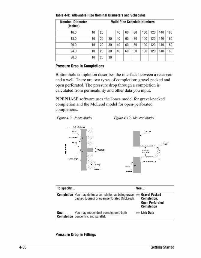
Pressure Drop in Completions

Bottomhole completion describes the interface between a reservoir and a well. There are two types of completion: gravel packed and open perforated. The pressure drop through a completion is calculated from permeability and other data you input.

PIPEPHASE software uses the Jones model for gravel-packed completion and the McLeod model for open-perforated completions.

Pressure Drop in Fittings

16.0 10 20 40 60 80 100 120 140 160

18.0 10 20 30 40 60 80 100 120 140 160

20.0 10 20 30 40 60 80 100 120 140 160

24.0 10 20 30 40 60 80 100 120 140 160

30.0 10 20 30

Figure 4-9: Jones Model Figure 4-10: McLeod Model


Completion You may define a completion as being gravel packed (Jones) or open perforated (McLeod).

➱ Gravel Packed Completion,Open Perforated Completion

Dual Completion

You may model dual completions, both concentric and parallel.

➱ Link Data

Table 4-8: Allowable Pipe Nominal Diameters and Schedules

Nominal Diameter (Inches)

Valid Pipe Schedule Numbers


The general form of the pressure drop equation is:

where:

ΔP = pressure drop across the fitting

K = resistance coefficient/ K-factor

G = mass velocity (mass flowrate/flow area)

Φ = two-phase pressure drop multiplier

g = acceleration due to gravity

ρ = fluid density (equal to liquid density for two-phase flows)


Bend, Tee,Valve

PIPEPHASE software uses the generalized pressure drop equation with a resistance coefficient. For bends, tees, and valves, you can either supply the resistance coefficient directly or supply an equivalent length and have PIPEPHASE software calculate the resistance coefficient as a function of the friction factor.

➱ Bend,Tee,Valve

Entrance Exit

For entrances and exits you can supply the resistance coefficient or use the default value.

➱ Entrance,Exit

Contraction, Expansion, Nozzle, Orifice, Venturi

For contractions, expansions, nozzles, orifices, and Venturimeters, you can supply the resistance coefficient or use the value that PIPEPHASE calculates from its built-in correlations. These correlations relate the resistance coefficient to the Reynolds number and specific fitting parameters such as orifice diameter, Venturi throat diameter, contraction and expansion angles, and nozzle diameter. For gas flow in nozzles, orifices, and Venturimeters, the specific heat ratio is also used in the calculation of the resistance coefficient.

➱ Nozzle, Expansion, Venturi, Contraction, Orifice

Choke The pressure drop for a choke is calculated by the orifice method for a single-phase fluid or by the Fortunati method for a two-phase fluid. You can supply a discharge coefficient or use the default value. MCHOKE, a variant of CHOKE which introduces a discontinuity into a network, uses the Fortunati model only.

➱ Choke Mchoke

Check Valve A valve that permits flow in one direction only. You can supply a resistance coefficient or use the default value.

➱ Check

Two-phase correction in fittings

The pressure drops for fittings are corrected for two-phase flow by using either the Homogeneous flow model or the Chisholm model. If you do not make a selection, PIPEPHASE software will use the default method. You may supply values for the Chisholm parameters.

➱ Bend, Exit, Entrance, Valve, Tee, Contraction, Expansion, Nozzle, orifice, Venturi

ΔP KG2Φ2gρ

----------------=


Equipment Items PIPEPHASE software simulates the change in fluid conditions across items of process equipment that typically appears in pipeline systems.


Compressor A compressor imparts work to a gas. You supply either a known power or a known outlet pressure, and PIPEPHASE software calculates the unknown parameter. You may impose a maximum value on the unknown parameter, and PIPEPHASE software will constrain the calculations according to whichever parameter is limiting. Alternatively, you can supply a curve of flowrate against head. You may also supply an adiabatic efficiency as either a constant or a curve against head. The exit temperature is then determined by energy balance. If you specify more than one stage, PIPEPHASE software interprets the curve to be for each stage; any maximum power you specify is over all of the stages rather than for each individual stage.

➱ Compressor

You can also reference the compressor curve to a previously defined performance curve.

➱ Compressor Curve Data, Compressor Performance Curves

Multispeed Compressor

You can specify different compressor curves for up to five compressor speeds.

➱ Compressor Curve Data

Multistage Compressor

In a multistage compressor you may specify different parameters – curves, efficiencies, etc.– for different stages. You may have multiple compressor trains, each train with multiple stages. You may have interstage scrubbers with downstream re-injection and interstage coolers and piping losses. You may specify the compressor’s inlet pressure. When you do this, PIPEPHASE software invokes a special algorithm which breaks the flowsheet at the compressor inlet and solves the resulting subnetworks so that the pressures match at the interface.

➱ Mcompressor

Cooler The cooler removes heat from the system. You supply either a known exit temperature or known duty of the unit, and PIPEPHASE software will calculate the unknown parameter. You may impose a maximum (for duty) or minimum (for temperature) value on the unknown parameter, and PIPEPHASE software will constrain calculations according to whichever parameter is limiting.

➱ Cooler

Steam Expander

The expander models the expansion of steam from a high pressure to a low pressure. You may specify the power required, or the pressure drop or the pressure ratio. If the unit is in a spur link, you may alternatively specify the outlet pressure.

➱ Expander


Gaslift Valve This unit simulates the presence of a gaslift valve as part of a well link. You must define the PVT properties of the lift gas.

➱ Gaslift Valve, Fluid Property Data

General purpose DP and DT unit

The DPDT unit is a general purpose unit for defining a pressure and/or temperature difference at a point in the piping structure. You can use this unit to model any equipment device where the pressure difference and temperature difference characteristics can be represented as curves against flowrate. You may also specify the flow versus pressure drop equation for the curve.

➱ DPDT

Heater The heater adds heat to the system. You supply either a known exit temperature or known duty of the unit, and PIPEPHASE software will calculate the unknown. You may impose a maximum value on the unknown parameter, and PIPEPHASE software will constrain the calculations according to whichever parameter is limiting.

➱ Heater

Injector The injector introduces a stream into a link. The stream comes from a separator (see the entry below). You may fix the pressure and temperature of the injected stream. The injector must be downstream of the separator and in the same link.

➱ Injector

Pump A pump imparts work to a liquid. You supply either a known power or a known outlet pressure, and PIPEPHASE software calculates the unknown. You may impose a maximum value on the unknown parameter, and PIPEPHASE software will constrain the calculations according to whichever parameter is limiting. Alternatively, you can supply a curve of flowrate against head. You may also supply an efficiency as a constant or as a curve against head. The exit temperature is determined by energy balance. If you specify more than one stage, PIPEPHASE software interprets the curve to be for each stage; any maximum power you specify is over all of the stages rather than for each individual stage.You can also reference the pump curve to a previously defined performance curve.

➱ Pump

Multispeed Pump

You can specify different pump curves for up to five pump speeds.

➱ Pump Curve Data, Pump Performance Curves

Electric Submersible Pump

An extension of the PUMP item allows you to model an electric submersible pump. In addition to all the features mentioned above, you may supply motor horsepower as a curve, either in tabular form or as coefficients of an equation. You may specify auxilliary power to be supplied to the pump. You may specify head degradation as a function of gas ingestion percentage, plus minimum submergence, casing head pressure, and vertical pressure gradient in the casing-tubing annulus due to the gas column. Refer also to Separator, below.

➱ Electric Submersible Pump



You can also reference the electric submersible pump curve to a previously defined ESP performance curve.

➱ Electric Submersible Pump Curve

Regulator The regulator is used to set the maximum pressure at some point in the pipeline structure. It allows flow in only one direction and can be used to prevent flow reversal within selected links in a network. As an extension to the regulator allows you to specify the inlet pressure, you may specify the compressor’s inlet pressure. When you do this, PIPEPHASE software invokes a special algorithm which breaks the flowsheet at the compressor inlet and solves the resulting subnetworks so that the pressures match at the interface.

➱ Regulator

Multi-network Regulator

You may specify the inlet pressure of this item. When you do this, PIPEPHASE software invokes a special algorithm which breaks the flowsheet at the inlet and solves the resulting subnetworks so that the pressures match at the interface. You may also specify the flowrate through the regulator.

➱ Regulator

Separator The separator splits out all or part of the gas or liquid phase of a multiphase fluid. In the case of a hydrocarbon system with water, you can select the hydrocarbon or aqueous phase instead of the total liquid phase. You specify the amount separated as an absolute flowrate or as a percentage of the phase. You can separate more than one phase in one separator. You can then reinject the separated streams at points downstream in the link using the Injector. You cannot impose a pressure drop on the separator.

➱ Separator

Bottomhole Separator

If a separator is positioned at the bottomhole below an electric submersible pump, you may either specify gas injection percentage or supply pump dimensions and have PIPEPHASE software calculate it.

➱ Separator

Hydrates Hydrates are solid mixtures of water and other small molecules. Under certain process conditions, particularly in the gas processing industry, hydrate formation may clog lines and foul process equipment. The HYDRATE unit operation predicts the pressure and temperature regime in which the process is vulnerable to hydrate formation. Calculations performed assume the presence of free water for hydrates to form. Possible hydrate formers include: methane through isobutane, carbon dioxide, hydrogen sulfide, nitrogen, ethylene, propylene, argon, krypton, xenon, cyclopropane, and sulfur hexafluoride. The effect of sodium chloride, methanol, ethylene glycol, di-ethylene glycol, and tri-ethylene glycol hydrate inhibitors can also be studied.

➱ Hydrate Unit Operation

Calculator The Calculator allows you to perform calculations on flowsheet information using FORTRAN-like syntax. The Calculator results can be transfered back to the Optimizer for use as an optimization objective parameter or constraint.

➱ Calculator



Heat Transfer CalculationsPIPEPHASE software performs an energy balance on pipes, risers, tubing, and annuli. The heat transfer depends on the fluid temperature, properties, and flowrate, the temperature and properties of the surrounding medium, and the heat transfer coefficient between the fluid and the medium. PIPEPHASE software does not model heat transfer to the surroundings for fittings and equipment devices (point devices).

The general equation for heat transfer from a flow device is:

where:

The overall heat transfer coefficient either is input or may be calculated from the constituent film coefficients and geometries.

For risers and annuli you must specify an overall heat transfer coefficient.

For a pipe or tubing you may supply an overall coefficient or you may request detailed heat transfer calculations. Detailed heat transfer calculations are invoked when you input any one of the parameters required to carry out the calculations.

Detailed Heat Transfer in Pipes and Tubing

For a pipe surrounded by soil, water, or air, you define the medium properties (and velocity of water or air). For a buried pipe, you enter the buried depth.

For tubings you enter data that describe the properties of the annuli and casings between the outside of the tubing and the inside of the hole.

Q = rate of heat transfer per unit length

U = overall heat transfer coefficient

A = outside surface area per unit length

DT = temperature difference between bulk fluid and outside medium


Pipes and Tubing

You may specify an overall coefficient or the properties of the surrounding medium. You can supply these values globally for all devices or for individual devices. You also supply the ambient temperature or geothermal gradient.

➱ Global Defaults Pipe Tubing

Q UAΔT=


Sphering or PiggingPIPEPHASE software’s sphering calculations predict the quantity of liquid formed when a multiphase fluid flows in a pipeline and determine the size of the liquid slug that is pushed out when the pipe is pigged.

Sphering calculations can only be carried out for single links. The launching station is at the inlet of a pipe. You may have intermediate launching stations; a sphere is launched from a pipe when the previous sphere(s) reach the inlet of that pipe.

Reservoirs and Inflow Performance RelationshipsUsing PIPEPHASE software, you can examine the effect of reservoir conditions on the performance of wells and downstream networks. You can also investigate the implications of declining reservoir pressure and production rate and shut-in wells when a user-specified maximum water cut or gas-oil ratio is exceeded.

Annuli and Risers

You specify the overall heat transfer coefficient and the geothermal gradient. You can supply these values globally for all devices or for individual devices.

➱ Global Defaults Annulus Riser

Isothermal calculations

For non-compositional gas or liquid fluid models, you may suppress heat transfer calculations for individual flow devices.

➱ Pipe Tubing Annulus Riser


Calculation type You must specify that you want to do a sphering simulation.

➱Network Calculation Methods

Fluid type The fluid must be compositional and both gas and liquid should be present to obtain realistic results.

➱Simulation Definition

Time Increments You may override the default time step used in the McDonald-Baker successive steady-state calculation method.

➱Network Calculation Methods

Structure Data You may have only PIPE devices. You identify a pipe with a launching station by specifying a sphere diameter for the pipe. The first launching station must be in the first pipe of the link.

➱ Pipe



The Inflow Performance Relationship device models the relationship between flowrate and reservoir pressure drawdown or pressure drop at the sand face in a well.

Production Planning and Time-SteppingProduction planning involves the study of the time-dependent interactions between the producing formation(s) and all of the wells, gathering lines, and surface facilities in an oil or gas field. PIPEPHASE software supplies this capability through its Time-stepping feature.

Typically, the study extends from a few years to the entire producing life of the field. For such extended periods, a quasi-steady state approach provides an efficient representation of the time-dependency. Time-stepping carries out a series of steady-state PIPEPHASE software simulations automatically in the same run. Each simulation represents the conditions at a specific time-step in the operating history of the field.


Type of model You may select from five standard models. You may write your own subroutine and use it to model the inflow performance relationship.

➱ IPR

Reservoir Curves

You may enter tables of reservoir pressure, cumulative production, Gas-Oil Ratio, Condensate-Gas Ratio, Water Cut, and Water-Gas ratio. These are used in Time-stepping to simulate reservoir decline with time.

➱ IPR

Multiple reservoirs and multiple wells

You can have up to twenty reservoirs in one network. One reservoir can serve several wells.

➱ IPR

Automatic subsurface networks

You may automatically create a subsurface network for a well with multiple sources. PIPEPHASE software solves these using a finite difference solution method. This is a quicker but less rigorous method of creating a subsurface network. Refer to Subsurface Networks and Multiple Completion Modeling on Page for further details.

➱ IPR

IPR curves You may enter curves that correlate reservoir pressure or cumulative production with flowing bottomhole pressure and flowrate. These data are then regressed onto one of the standard models.

➱ IPR

Pseudo-pressure formulation

For an IPR with a gas basis, you may specify a drawdown formulation.

➱ IPR

Well Shut-in Controls

You may supply the maximum water cut or gas-oil ratio for well shut-in.

➱ IPR

You can also specify the priority of well shut-in for multiple wells.

➱ Source


Wells and Well Grouping

Each of the well completion zones in a gathering network produces from a specific formation or reservoir. The decline in the reservoir pressure with time and the changes in the characteristics of the fluid produced are a function of the total fluid volume produced from the reservoir. For the purposes of these calculations, a well completion is associated with a reservoir group. A reservoir group includes all of the producing zones that contribute to its depletion.

Reservoir Depletion

The depletion of a reservoir over the life of a field is characterized by a decline in average reservoir pressure and changing fluid composition. For most reservoirs, the gas-oil ratio increases with time; for a reservoir with an active water drive, the produced water cut increases as the water table rises.

Facilities Planning

In a gathering system, changes to the operation of surface facilities directly affect the overall production. For example, adding compression facilities to an existing gas gathering network reduces the pressure at the upstream wells, which in turn increases the drawdown and results in improved production from the reservoir; an increase in the separator pressure will have the opposite effect. Time-stepping enables you to simulate changes to the facilities installation over time.


Reservoir Groups

You must name the reservoir GROUP and supply depletion data in one IPR device. Other IPR devices may access the same reservoir depletion data by using the same GROUP name.

➱ IPR

Depletion characteristics

Supply a curve of reservoir pressures against cumulative production.

➱ IPR

Gas and gas condensate fields

For a gas or gas condensate field you may supply the slope of the depletion curve as pressure decline rate per unit of production.

➱ IPR

Production decline rates for each IPR

The production decline characteristics for individual completion zones must be defined. Tabular data represent the decline in the flowing well pressure as a function of the production rate. The time-dependent parameter may be expressed in terms of reservoir pressure or cumulative production.

➱ IPR

Fluid compositional changes

You may enter curves for water cut, gas-oil ratio (or condensate-gas ratio for condensate wells), and water cut (or water-gas ratio for condensate wells) as functions of reservoir pressure or cumulative reservoir produced volume.

➱ IPR


Subsurface Networks and Multiple Completion ModelingA Single Well

A single well can produce from one reservoir:

Figure 4-11: One Well, One Reservoir

Or a single well can produce from more than one reservoir:

Selecting times

Supply a series of times. PIPEPHASE software will carry out simulations at each of those times.

➱ IPR

Downstream network changes

At each time you may specify one or more changes to the network or conditions downstream of the well.

➱ IPR

To specify: See...

A source to give the properties, flowrate, and conditions of the fluid. ➱ Source

One IPR to define the interface to the reservoir. ➱ IPR

One tubing from the well to the surface. ➱ Tubing

One node to continue into the rest of the network. ➱ Junction, Sink

To specify: See...

A source for each reservoir to give the properties, flowrates, and conditions of the fluids.

➱ Source

An IPR for each reservoir to define the interfaces. ➱ IPR

A tubing between consecutive reservoirs. ➱ Tubing

A tubing from the last reservoir to the surface. ➱ Tubing

A node to continue into the rest of the network. ➱ Junction, Sink



Figure 4-12: One Well, More Than One Reservoir

More Than One Well

You may have more than one well in a PIPEPHASE software run. The wells may all use one reservoir. In this case, information for the reservoir data is entered in one IPR and accessed from other IPRs using the GROUP name.

Multiple Completions

In PIPEPHASE software you may model a multiple completion rigorously:

To specify: See...

A source for each completion to give the properties, flowrates, and conditions of the fluids.

➱ Source

An IPR for each completion to define the interfaces. ➱ IPR

Tubing and junctions to form the network between completions. ➱ Tubing

A tubing from the last completion to the surface. ➱ Tubing


Tubing

Ground Level

Reservoir

Tubing

Reservoir

Junction or sink

IPR

IPR

Subsurface junction


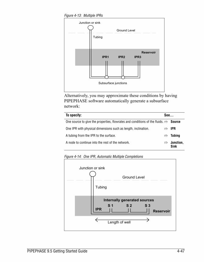
Figure 4-13: Multiple IPRs

Alternatively, you may approximate these conditions by having PIPEPHASE software automatically generate a subsurface network:

Figure 4-14: One IPR, Automatic Multiple Completions

To specify: See...

One source to give the properties, flowrates and conditions of the fluids. ➱ Source

One IPR with physical dimensions such as length, inclination. ➱ IPR

A tubing from the IPR to the surface. ➱ Tubing


Reservoir

IPR1 IPR2 IPR3

Tubing

Ground Level

Junction or sink

Subsurface junctions

Reservoir

Length of well

S 1 S 2 S 3

Internally generated sources

IPR

Tubing

Ground Level

Junction or sink


Case StudiesThe Case Study option provides the facility to perform parametric studies and to print multiple problem solutions in a single computer run. Case studies are always performed after the base case problem has been solved. If the base case problem cannot be solved for any reason, then no case studies are performed. Each case study analysis is performed based on the cumulative changes to the flowsheet up to that time.

Case studies are an efficient means of obtaining solutions for multiple scenarios to a given problem and result in large savings in both computer time and cost. For problems requiring iterative solutions, the converged results of the last solution are used as the starting values for the next run. This can result in large computer time savings in runs involving large networks, where it typically takes several iterations to move from the initial pressure estimates to the final converged solution.

There is no limit on the number of changes you can make per case study or on the total number of case studies that may be in a given run. The cumulative changes up to a given case study run may be erased and the original base case restored at any time.

Since the case studies are performed sequentially in the order you input, it is best to make changes in an orderly manner, proceeding from high values to low values or low values to high values, but not in a random order. This enhances convergence and minimizes total computer time. See Chapter 4, Input Reference, Table 4-46 in PipePhase Keyword Manual.

Global Changes

You may change one parameter in the entire problem using a global command. You do this by supplying the type of parameter you want to change, its old value, and the new value. Only those specified parameters with that old value will then be changed.

The items to which this type of change can be applied are identified in Table 4-46, Chapter 4, Input Reference in PipePhase Keyword Manual.


Individual Changes

Source, sink, and device parameters may be changed individually. You must specify a name for each source, sink, or device where a parameter change is desired.

To... See...

Add descriptive text

You can add one line of description for each case study.

➱Simulation Description

Make changes You can change any of the parameters in Table 3-7, either globally or on individual flow elements.

➱Case Study Changes

You can restore the base case at any time. ➱Case Study Changes

Table 4-9: Changes allowed in Case Studies

Flow Device Parameter Type of Change

Pipe LENGTHECHGIDROUGHNESSUTAMBIENTFCODE

Global IndividualGlobal IndividualGlobal IndividualGlobal IndividualGlobal IndividualGlobal IndividualGlobal Individual

Riser IDROUGHNESSUFCODE

Global IndividualGlobal IndividualGlobal IndividualGlobal Individual

Tubing IDROUGHNESSUFCODETGRAD

Global IndividualGlobal IndividualGlobal IndividualGlobal IndividualGlobal Individual

Annulus IDANNODTUBROUGHNESSUFCODETGRAD

Global IndividualGlobal IndividualGlobal IndividualGlobal IndividualGlobal IndividualGlobal Individual

Compressor/Pump

POWERPRESSUREEFFICIENCYSTAGES

Global IndividualGlobal IndividualGlobal IndividualGlobal Individual

Heater/Cooler DUTYTOUTDP

Global IndividualGlobal IndividualGlobal Individual

Choke IDCOEFFICIENT

Global IndividualGlobal Individual

Sales RATE Global Individual


Nodal AnalysisNodal Analysis allows you to study the overall performance of wells, pipelines and other single link systems as a function of input parameters and flowrates. The results are summarized in tabular and graphical form. You can also study combinations of inflow and outflow parameters using the multiple combination nodal analysis option.

Nodal Analysis is performed on a single link.

Dividing the Link

You first divide your single link into two sections, separated by a Solution Node. The section upstream of the Solution Node is called the Inflow section and would typically be the tubing of a well. The section downstream of the Solution Node is called the Outflow section and would typically be the flowline from the wellhead to a surface separator. The Solution Node, in this case, would be the well-head node.

If you locate the Solution Node actually at the source or the sink, then there will be only an Outflow or Inflow section respectively.

Source PRESSURETEMPERATURERATEQUALITYCOMPOSITIONCGRCOEFFICIENTEXPGORPIVOGELWCUTWGR

IndividualIndividualIndividualIndividualIndividualIndividualIndividualIndividualIndividualIndividualIndividualIndividualIndividual

Sink PRESSURERATEII

IndividualIndividualIndividual

Completion SHOTSPERFPENETRATIONTUNNEL

General IndividualGeneral IndividualGeneral IndividualGeneral Individual

GLValve DISSOLVERATE

General IndividualGeneral Individual

Table 4-9: Changes allowed in Case Studies

Flow Device Parameter Type of Change


If you do not want to vary any parameters in either the Inflow section or the Outflow section, simply omit these sections. Obviously, a Nodal Analysis cannot be carried out without at least one of these sections.

Selecting Parameters and Flowrates

You then select a parameter in the Inflow section and a parameter in the Outflow section. Typical parameters would be reservoir pressure (for Inflow) and pipe ID (for Outflow). You may enter up to five values for each of these parameters. Each combination of Inflow parameter value and Outflow parameter value represents an operating point of the system. This means that there may be up to 25 operating points.

The parameters you select must have values supplied in the base case input data.

Finally, you define up to ten flowrates.

Nodal Results

PIPEPHASE software calculates the flowrates and Solution Node pressures corresponding to each operating point and prints them out in the form of tables and plots. The flowrates you input must span all the flowrates at which you expect the operating points to occur.

Grouping Parameters

As an extension to the Nodal Analysis feature, PIPEPHASE software allows you to group a number of variables into one nodal parameter. For example, you may define an Outflow parameter as a combination of pump power, pipe ID and heater temperature. Each of the five values of the Outflow parameter would now be a combination of the corresponding values of each of the contributing variables.

Thus you might define that the first value of the Outflow parameter is the combination of 25KW pump power with 30 mm pipe ID and 400 K; the second 30KW, 40 mm and 310 K; the third 35KW, 50 mm and 350 K; and so on.

To... See...

Add descriptive text

You can add one line of description for each of the Inflow and Outflow sections.

➱ Simulation Description


Define the Solution Node

You must define a Solution Node which comes between the Inflow and Outflow sections. If you want the Solution Node to be at the flowing bottomhole of an injection well, use BOTTOMHOLE. If you want to locate the Solution Node at the outlet of the last device and want to use Sink pressure as a variable parameter, use SINK.

➱ Link Device Data, Nodal Analysis

Define the parameter(s)

You must define at least one Inflow or Outflow parameter for PIPEPHASE software to change. The parameters that are accessible are divided into seven categories, as defined in the table below. If you want to define a nodal parameter as a group of variables, you may combine up to ten variables within one Category. You may not combine variables in different categories.

➱ Nodal Analysis Parameters

Study multiple combinations of parameters

You can specify up to four — two inflow and two outflow — parameters for the multiple combinations option. You can then supply up to five values of each parameter. PIPEPHASE software will combine each of the up to five values of an inflow or outflow parameter with each of the up to five values of the second inflow or outflow parameter and so on and will present the results of the analysis of the combined variables.

➱ Nodal Analysis

Table 4-10: Variables Available to Nodal AnalysisCategory Device Variable

Category 1 - Source SOURCE NAMEPRESSURECOEFFICIENTEXPPIVOGEL

Category 2 - Sink SINK NAMEPRESIICOEFFEXP

Category 3 - Devices PIPE NAMEIDROUGHNESSUFLOWEFF

RISER NAMEIDROUGHNESSUFLOWEFF

TUBING NAMEIDROUGHNESSUFLOWEFF

To... See...


ANNULUS NAMEIDANNODTUBROUGHNESSUFLOWEFF

COMPRESSOR/PUMP NAMEPOWERPRESSUREEFFICIENCYSTAGES

HEATER/COOLER NAMEDUTYTOUTDP

CHOKE NAMEIDCOEFFICIENT

SEPARATOR NAMERATEPERCENT

GLVALVE NAMERATEDISSOLVE

INJECTOR NAMETEMPERATUREPRESSURE

COMPLETION NAMEPENETRATIONPERFDSHOTSTUNNEL

Category 4 - Non-compositional Source Properties

GORWCUTCGRWGRQUALITY

Category 5 - Main Source COMPOSITION

Table 4-10: Variables Available to Nodal AnalysisCategory Device Variable


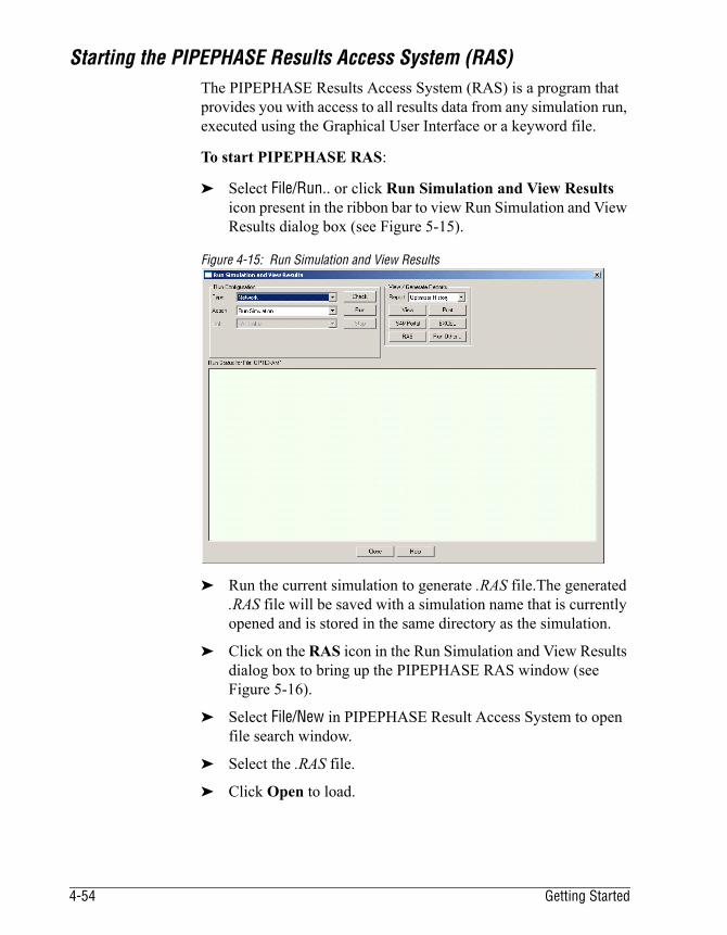
Starting the PIPEPHASE Results Access System (RAS)The PIPEPHASE Results Access System (RAS) is a program that provides you with access to all results data from any simulation run, executed using the Graphical User Interface or a keyword file.

To start PIPEPHASE RAS:

➤ Select File/Run.. or click Run Simulation and View Results icon present in the ribbon bar to view Run Simulation and View Results dialog box (see Figure 5-15).

Figure 4-15: Run Simulation and View Results

➤ Run the current simulation to generate .RAS file.The generated .RAS file will be saved with a simulation name that is currently opened and is stored in the same directory as the simulation.

➤ Click on the RAS icon in the Run Simulation and View Results dialog box to bring up the PIPEPHASE RAS window (see Figure 5-16).

➤ Select File/New in PIPEPHASE Result Access System to open file search window.

➤ Select the .RAS file.

➤ Click Open to load.


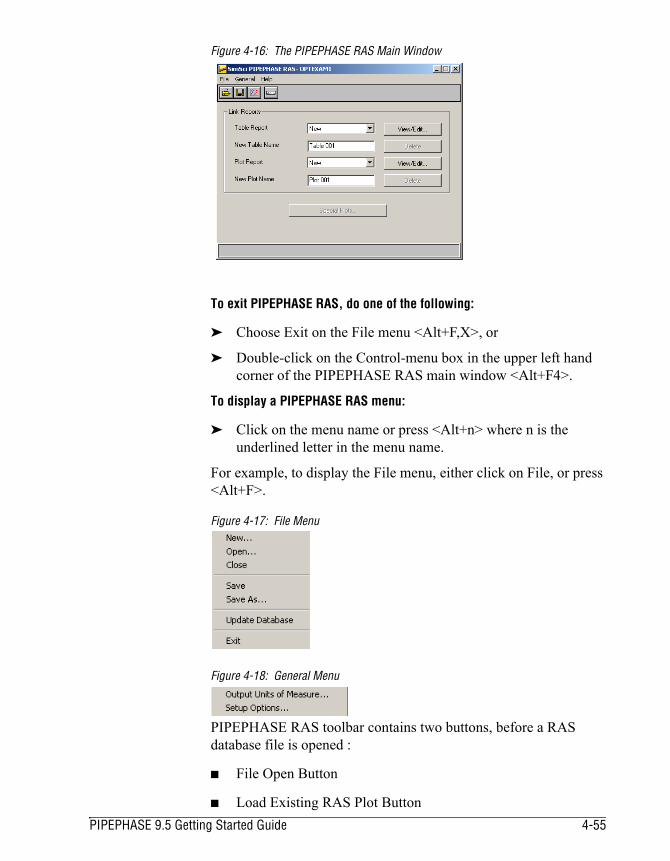
Figure 4-16: The PIPEPHASE RAS Main Window

To exit PIPEPHASE RAS, do one of the following:

➤ Choose Exit on the File menu <Alt+F,X>, or

➤ Double-click on the Control-menu box in the upper left hand corner of the PIPEPHASE RAS main window <Alt+F4>.

To display a PIPEPHASE RAS menu:

➤ Click on the menu name or press <Alt+n> where n is the underlined letter in the menu name.

For example, to display the File menu, either click on File, or press <Alt+F>.

Figure 4-17: File Menu

Figure 4-18: General Menu

PIPEPHASE RAS toolbar contains two buttons, before a RAS database file is opened :

■ File Open Button

■ Load Existing RAS Plot Button

Two additional buttons appear on the toolbar, after a RAS database file is opened:

■ Save RAS Database

■ Define Output Units of Measure

Starting the PIPEPHASE Excel ReportPIPEPHASE software has extended its capability in the area of generating reports by providing an Excel spreadsheet format to its entire simulation. In this enhancement, ACCESS database was duly expanded to include all the data available in the simulation. So that user can be provided with all the required information in an Excel spreadsheet format.

Procedure to invoke Excel report has been listed below:

➤ Select Generate Excel Report.. option in View Output Menu or click Excel Reports icon in the toolbar to generate an Excel report for a currently opened simulation. Excel Reports dialog box (see figure 5-19) will pop up on selecting this option.

Figure 4-19: Excel Reports

➤ In the Excel Reports dialog box, different types of Summary and Line reports available to generate will be listed. You can observe some of the options have been already selected. The selected options are called Set default ‘Print Options’. User is expected to select the required options from the list that is to be made available in the Excel Report to be generated.


➤ Clicking Set default ‘Print Options’ will automatically reselect the default reports available for the current simulation.

➤ Select all the options listed under Run Options.

➤ Click Run Current Network to execute the options checked under Run Options. This will generate Excel Reports for the simulation, which is currently opened.

➤ Excel Reports will be generated only if you have run the simulation and created database for the simulation.

➤ To view previously generated report for the current simulation, select View Excel Reports in View Output menu. If the previously generated report is not available for the current simulation, then an error message will pop up requesting the user to generate an Excel report.

To generate and view Excel Reports for a Batch of Simulation files:

➤ Click Edit Simulation List... to open General Spread Sheet - Batch Run files dialog box (See figure 5-20).

Figure 4-20: General Spreadsheet - Batch Run Files

Note: Uncheck the Run Simulation option under Run Options, if you have already run the simulation through Run Simulation and View Results dialog box. Excel Reports dialog box can be viewed by clicking Excel button present in Run Simulation and View Results dialog box (see Figure 5-15).


➤ Click Append Row to open a Search window. This window searches .inp files in the default disk/directory. You may change to a different directory or disk to search a particular file.

➤ Select the appropriate file and click Open.

➤ Now you can find the selected file has been listed in the General Spread Sheet – Batch Run Files dialog box. Similarly user can append number of files using General Spread Sheet – Batch Run Files dialog box by clicking Append Row.

➤ Similarly, the files can be added by clicking Insert Row.

➤ Click Delete Row to delete an Appended/Inserted file.


➤ Click Run Simulation List to execute the options checked under Run Options. This will generate Excel Reports for the listed simulation.


Chapter 5Tutorial

IntroductionThis chapter presents the step-by-step procedure required for the optimization of an off-line pipeline design. In the first part of this tutorial, you will look at the optimal design based only on capital cost considerations. Then, you will include the operating costs over the lifetime of the pipeline (10 years) and examine the effect the operating costs have on the overall design strategy.

Problem DescriptionIn this simulation, a pipeline is designed to deliver gas at a rate of 1200 MMSCFD at a minimum pressure of 900 psi from two offshore fields. Table 5-1 and Table 5-2 provide additional process details including piping and compressor capital expenditures.

Table 5-1: Process Conditions

Offshore Field A

Distance from processing plant, miles 200(1056000 feet)

Wellhead pressure, psi 2000

Offshore Field B

Distance from field A, miles 180(950400 feet)

Wellhead pressure, psi 2000

Table 5-2: Pipeline and Compressor Capital Costs

Pipeline Cost/mile $0.70MM/inch ID

Compressor Cost/1000 hP $4.66MM


The overall capital cost is the sum of the cost of purchasing and laying pipe and purchasing the compressors.

The overall capital cost is therefore a linear function of the ID of the two pipeline segments and compressor power:

PIPEPHASE software optimizes the design to minimize the overall capital costs by varying the pipe diameters and the sizes of the compressors at the two platforms. Apart from the delivery target, there are three additional design and operating constraints that must be taken into consideration:

■ Pipe sizes are available only in sizes 24"-40" with a maximum operating pressure of 2475 psi.

■ Due to limited space on each platform, the maximum capacity of each compressor is 50000 HP.

■ Both pipeline sections must be built as the capacity of the plat-form for field A is inadequate to meet the overall delivery requirement.

The overall network is shown in Figure 5-1.

Pipe Costs (MM$) = Cost of Pipe from Field 1 + Cost of Pipe from Field 2

= 0.70*200*IDPipe 1 + 0.70*180*IDPipe 2

= 140*IDPipe 1 + 126*IDPipe 2

Compressor Cost (MM$) = 4.66E-3*wCompr 1 + 4.66E-3*wCompr 2

Capital Cost =140*IDPipe 1 + 126*IDPipe 2 + 4.66E-3*wCompr 1 + 4.66E-3*wCompr 2

5-2 Tutorial

Figure 5-1: Tutorial Problem

Building the NetworkFirst, you must open a new project:

➤ Select the New option from the File menu. The Windows explorer dialog box is displayed. Next, you must supply a name for this new simulation.The Create New Simulation window appears for laying down your process flowsheet. By default, this simulation will be created in the C:\SIMSCI\PPHASE95\USER directory.

➤ Type ‘optexam1’ in the File Name data entry field as shown in Figure 5-2.

➤ Then, click the Open button.


Figure 5-2: Create New Simulation Window

Tip:By using the toolbar icons, you reduce the number of mouse actions required for a selection. For example, you can click the toolbar button to create a new simulation.

PIPEPHASE software will now automatically take you through Simulation Setup Wizard .

Figure 5-3: Welcome to Simulation Setup Wizard

➤ Click the Next button.

5-4 Tutorial

Figure 5-4: Select Simulation Type

➤ Select the Network model Simulation Type.


Figure 5-5: Select Fluid Type

➤ Select Gas as Fluid Type.



Figure 5-6: Select Default Units of Measurement

➤ Select Petroleum as Default Units of Measurement.


Figure 5-7: Confirm the Selections

➤ Confirm your selections.

➤ Click on Finish.The Fluid Property Data window will appear as shown in Figure 5-8.

➤ Click Edit on the Fluid Property Data window.

➤ The Single Phase Gas PVT Data window will then appear.

5-6 Tutorial

➤ Enter a specific gravity of 0.69 in the Gas Gravity field and the following composition of contaminants:

The completed window will appear as shown in Figure 5-9.

Figure 5-8: Fluid Property Data

➤ Click the OK button to continue.

Figure 5-9: Single Phase Gas PVT Data Window

Component Mole %

Nitrogen 1.32

Carbon dioxide 0.98

Hydrogen sulfide 0.56


To create a second property data set.

➤ Click the New button on Fluid Property Data window. This brings up the Single Phase Gas PVT Data window with Set Number already set to 2.

➤ Enter a specific gravity of 0.701 in the Gas Gravity field and the following composition of contaminants:

The completed window will appear as shown in Figure 5-10.

Figure 5-10: Single Phase Gas PVT Data Window

➤ Click the OK button. The Fluid Property Data window will appear as shown in Figure 5-11.

Component Mole %

Nitrogen 1.11

Carbon dioxide 0.88

Hydrogen sulfide 0.24

5-8 Tutorial

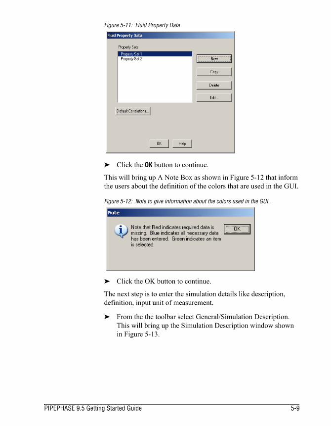
Figure 5-11: Fluid Property Data


This will bring up A Note Box as shown in Figure 5-12 that inform the users about the definition of the colors that are used in the GUI.

Figure 5-12: Note to give information about the colors used in the GUI.


The next step is to enter the simulation details like description, definition, input unit of measurement.

➤ From the the toolbar select General/Simulation Description. This will bring up the Simulation Description window shown in Figure 5-13.


Figure 5-13: Simulation Description Window

To complete this data entry window:

Enter the Project, Problem, User, Date, Site, and Description data entry fields and click the OK button.

➤ From the toolbar select General/Simulation Definition. This will bring up the Simulation Description window shown in Figure 5-14.

➤ Use the drop-down list boxes to select a Simulation Type of Network Model and a Fluid Type of Gas.

Figure 5-14: Simulation Definition Window


After leaving the Simulation Definition window, you will want to check Input Dimensions. From the the toolbar select General/Input Units of Measurement. This will bring up the Input Dimensions window shown in Figure 5-15.

5-10 Tutorial

➤ Use the Input Units of Measurement window to change the default units of various parameters like Oil Density, Pipe Length, etc as shown in Figure 5-15.

Figure 5-15: Input Dimensions Window


The next step is to begin entering the nodes _ sources, sinks, and junctions _ required for the problem. For this simulation, you will lay down two sources, one sink, and one junction, in that order.

To select the nodes:

➤ Click one of the node icons from the toolbar.

➤ Move the cursor to the location on the main window where the node is to be located and click again. The node will appear in the main flowsheet area of the screen.

➤ Repeat this step for each of the nodes in the flowsheet until the entire system has been constructed as shown in Figure 5-16.

For the source node

For the sink node

For the junction


Figure 5-16: PIPEPHASE Main Window

Tip:For very large systems, multiple nodes may be placed by holding down the Shift key and clicking on each desired location for a given node.

All of the source and sink nodes placed on the screen should be bordered in red indicating that user input is required for that node.

After all of the nodes have been placed and named as shown in Figure 5-16, the next step is to connect the nodes into a logical flow network.

Note: If you have added the nodes in the stated order of sources, sink, followed by the junction, the sources will be labeled S001 and S002, the sink, D001, and the junction, J001. Also, Figure 5-16 refer to the Applib file ‘optexam1’ which is available in the user directory (\\PPhase95\User\Samples\Optimizer) and all the units, devices and links provided refer to the Applib file.

Note: Once a node has been placed, it may be moved by simply clicking on the node with the left mouse button, holding it down, and dragging the node to a new location.

5-12 Tutorial

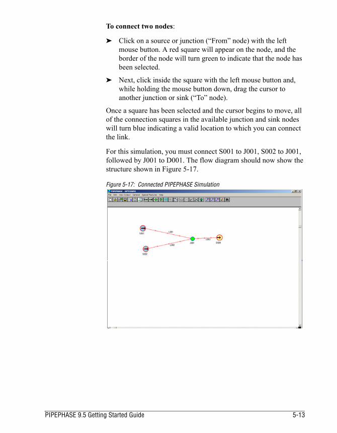
To connect two nodes:

➤ Click on a source or junction (“From” node) with the left mouse button. A red square will appear on the node, and the border of the node will turn green to indicate that the node has been selected.

➤ Next, click inside the square with the left mouse button and, while holding the mouse button down, drag the cursor to another junction or sink (“To” node).

Once a square has been selected and the cursor begins to move, all of the connection squares in the available junction and sink nodes will turn blue indicating a valid location to which you can connect the link.

For this simulation, you must connect S001 to J001, S002 to J001, followed by J001 to D001. The flow diagram should now show the structure shown in Figure 5-17.

Figure 5-17: Connected PIPEPHASE Simulation


The next step is to enter the data for each of the sources and sinks. To enter the data for the source S001:

➤ Double-click on the node S001, and enter the following information:

➤ Select the PVT Property Set as 1 in the Properties field. The window should appear as shown in Figure 5-18.

Figure 5-18: Completed Gas Source S001 Window

➤ Click the OK button to return to the main window. The source is now bordered in blue, indicating that all required data have been entered.

To enter the data for the source S002:

➤ Double-click on the node S002. The same window should appear as shown in Figure 5-18.

Node Data Value

Pressure (fixed) 2000 psig

Temperature 80 F

Standard Flowrate (estimated) 600 MMft3/day

5-14 Tutorial

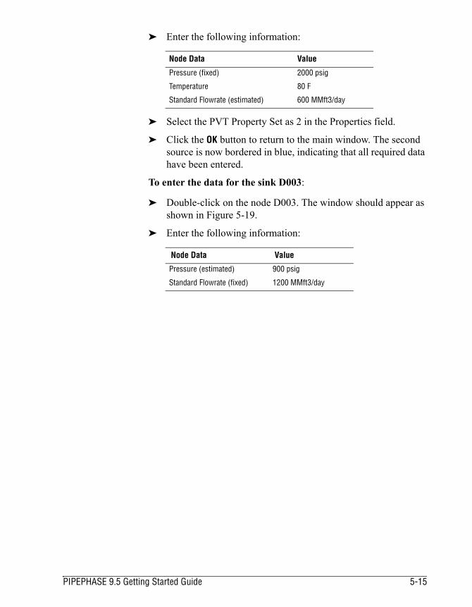
➤ Enter the following information:

➤ Select the PVT Property Set as 2 in the Properties field.

➤ Click the OK button to return to the main window. The second source is now bordered in blue, indicating that all required data have been entered.

To enter the data for the sink D003:

➤ Double-click on the node D003. The window should appear as shown in Figure 5-19.

➤ Enter the following information:

Node Data Value

Pressure (fixed) 2000 psig

Temperature 80 F

Standard Flowrate (estimated) 600 MMft3/day

Node Data Value

Pressure (estimated) 900 psig

Standard Flowrate (fixed) 1200 MMft3/day


Figure 5-19: Completed Sink D003 Window

➤ Click the OK button to return to the main window. The sink is now bordered in blue, indicating that all required data have been entered.

➤ Lastly, you must enter the data for each of the links on the flowsheet. Let’s start with link L001 between source S001 and junction J004.

To enter the data for this link:

➤ Double-click on the link L001. This brings up the Link <L001> Device Data window as shown in Figure 5-20.

5-16 Tutorial

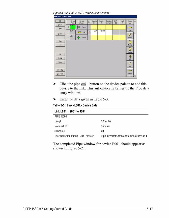
Figure 5-20: Link <L001> Device Data Window

➤ Click the pipe button on the device palette to add this device to the link. This automatically brings up the Pipe data entry window.

➤ Enter the data given in Table 5-3.

The completed Pipe window for device E001 should appear as shown in Figure 5-21.

Table 5-3: Link <L001> Device Data

Link L001 _ S001 to J004

PIPE E001

Length 0.2 miles

Nominal ID 8 inches

Schedule 40

Thermal Calculations Heat Transfer Pipe in Water; Ambient temperature: 45 F


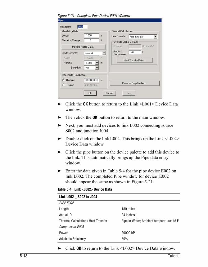
Figure 5-21: Complete Pipe Device E001 Window

➤ Click the OK button to return to the Link <L001> Device Data window.

➤ Then click the OK button to return to the main window.

➤ Next, you must add devices to link L002 connecting source S002 and junction J004.

➤ Double-click on the link L002. This brings up the Link <L002> Device Data window.

➤ Click the pipe button on the device palette to add this device to the link. This automatically brings up the Pipe data entry window.

➤ Enter the data given in Table 5-4 for the pipe device E002 on link L002. The completed Pipe window for device E002 should appear the same as shown in Figure 5-21.

➤ Click OK to return to the Link <L002> Device Data window.


Link L002 _ S002 to J004

PIPE E002

Length 180 miles

Actual ID 24 inches


Compressor E003

Power 20000 hP

Adiabatic Efficiency 80%

5-18 Tutorial

➤ Next, you must add a compressor to this link by clicking the compressor button on the device palette. This automatically adds this new device after the currently selected device (i.e., the pipe E002) and brings up the Compressor data entry window for device E003.

➤ Enter the data given in Table 5-4 for the compressor device E003 on link L002. The completed Compressor window should appear as shown in Figure 5-22.

Tip:To copy or delete a device previously added to a link, highlight that device, then click on the COPY then PASTE or DELETE buttons on the left palette in the Link Device Data window.

Figure 5-22: Completed Compressor E003 Window

➤ Click OK to return to the Link <002> Device Data window.

➤ Then, click OK again to return to the main window.

➤ Using the data given in Table 5-5, repeat the above steps for link L003 connecting junction J004 to sink D003. The main window will now appear as shown in Figure 5-23.


Link L003 _ J004 to D003

PIPE E004

Length 200 miles

Actual ID 35 inches


Compressor E005

Power 25000 hP


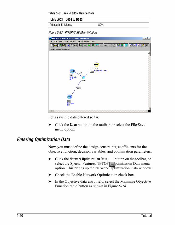
Figure 5-23: PIPEPHASE Main Window

Let’s save the data entered so far.

➤ Click the Save button on the toolbar, or select the File/Save menu option.

Entering Optimization DataNow, you must define the design constraints, coefficients for the objective function, decision variables, and optimization parameters.

➤ Click the Network Optimization Data button on the toolbar, or select the Special Features/NETOPT Optimization Data menu option. This brings up the Network Optimization Data window.

➤ Check the Enable Network Optimization check box.

➤ In the Objective data entry field, select the Minimize Objective Function radio button as shown in Figure 5-24.

Adiabatic Efficiency 80%


Link L003 _ J004 to D003

5-20 Tutorial

Figure 5-24: Network Optimization Window

➤ Now, you must define the objective parameters by clicking on the Objective Parameters button to bring up the Network Optimization Objective Parameters window.

As discussed previously, the overall capital cost is a linear function of the ID of the two pipeline segments and compressor power:

There are therefore four objective parameters for this optimization problem as shown in Table 5-6.

To enter the first objective parameter:

➤ In the Network Optimization Objective Parameters window, click the Add button. This brings up the Define Objective Parameter window.

➤ Select the Link Name radio button in the Node/Device/Calculator Name field.

➤ Select link L003 from the Link Name drop-down list box.

Capital Cost = 140*IDPipe 1 + 126*IDPipe 2 + 4.66E-3*wCompr 1 + 4.66E-3*wCompr 2

Table 5-6: Objective Parameters

Link Description Coefficient in Objective Function

L003 Pipe E004 Inside Diameter, ID 140

L002 Pipe E002 Inside Diameter, ID 126

L003 Compressor E005 Power, w 4.66E-3

L002 Compressor E003 Power, w 4.66E-3


➤ Select Pipe from the Device Type drop-down list box. By default, PIPEPHASE software will display the correct device name, E004.

➤ Select Inside Diameter from the Parameter drop-down list box.

➤ Type in 140 in the Correlation Coefficient data entry field as shown in Figure 5-25.

Figure 5-25: Define Objective Parameter Window

➤ Repeat for the other three objective parameters using the data in Table 5-6.

Tip:For the Compressor objective parameters, select Set Power from the Parameters drop-down list box in the Define Objective Parameter window.

➤ The completed Network Optimization Objective Parameters window is shown in Figure 5-26.

5-22 Tutorial

Figure 5-26: Network Optimization Objective Parameters Window

➤ Click the OK button to return to the Network Optimization Data window.

➤ Next you must define the decision variables.

There are four decision variables for this optimization problem as shown in Table 5-7 below.

To enter the first decision variable:

➤ In the Network Optimization Data window, click the Add button. This brings up the Define Decision Variable window.

➤ Select the Link Name radio button in the Node/Device Name field.

➤ Select link L003 from the Link Name drop-down list box.

➤ Select Pipe from the Device Type drop-down list box. By default, PIPEPHASE software will display the correct device name, E004.

➤ Select Inside Diameter from the Parameter drop-down list box.

➤ Click the Limits button. This brings up the Optimizer Variable Limits window as shown in Figure 5-27.

Table 5-7: Decision Variables

Link Description Limits Relative Perturbation

L003 Pipe E004 Internal Diameter, ID 24”<ID<48” -

L002 Pipe E002 Internal Diameter, ID 24”<ID<48” -

L002 Compressor E003 Power, w 0 hP<w<50000 hP 0.001

L003 Compressor E005 Power, w 0 hp<w<50000 hP 0.001


➤ In the Variable Lower Limit field, enter a value of 24 for Mechanical Limit (Absolute Value).

➤ In the Variable Upper Limit field, enter a value of 48 for Mechanical Limit (Absolute Value).

Figure 5-27: Optimizer Variable Limits Window

➤ Click the OK button to return to the Define Decision Variable window.

➤ Then, click the OK again to return to the Network Optimization Data window.

➤ Repeat for the other three decision variables using the data in Table 5-7 above.

Tip:For the Compressor decision variables, select Available Power from the Parameters drop-down list box in the Define Decision Variable window.

The Network Optimization Data window should now appear as shown in Figure 5-28.

5-24 Tutorial

Figure 5-28: Network Optimization Data Window

➤ Next you must define the constraints by clicking the Constraints button to bring up the Network Optimization Constraints window

To enter the first constraint:

➤ In the Network Optimization Constraints window, click the Add button. This brings up the Define Constraint window.

➤ Select the Node Type radio button in the Node/Device/Calculator/External Name field.

➤ Select Sink from the Node Type drop-down list box. By default, PIPEPHASE software will display D003 as the Node Name.

➤ Select Pressure from the Parameter drop-down list box.

➤ Click the Limits button. This brings up the Optimizer Variable Limits window.

➤ In the Variable Lower Limit field, enter a value of 900 for Mechanical Limit (Absolute Value).

➤ Click the OK button to return to the Define Constraint window.

Table 5-8: Constraints

Node Name Description Limits

Sink D003 Pressure P>900 psi

Link L002 Compressor E003 Outlet Pressure, P 0 psi<P<2475 psi

Link L003 Compressor E005 Outlet Pressure, P 0 psi<P<2475 psi


➤ Then click OK again to return to the Network Optimization Data window.

➤ Repeat for the other two constraints using the data in Table 5-8.

Tip:For the Compressor constraints, select Outlet Pressure from the Parameter drop-down list box in the Define Constraint window.

The Network Optimization Constraints window should now appear as shown in Figure 5-29.

Figure 5-29: Network Optimization Constraints Window

➤ Finally, you must specify the optimization options. Click OK to return to the Network Optimization Data window.

➤ On the Network Optimization Data window, click the Optimization Options button. This brings up the Optimization Options window. For this problem, you must increase the number of optimizer iterations from the default value of 10.

➤ In the Maximum Number of Optimizer Cycles field, select the Specified Number radio button and enter a value of 30 in the corresponding data entry field as shown in Figure 5-30.

➤ You can change the other Optimization parameters to the following values:

● Number of Cycles with Damping : 5

● Minimum relative change in objective function : 1.00E -04

● Minimum relative change in decision variable: 1.00E -03

● Default relative purturbation for derivatives: 0.04

● Minimum error in constraint : -0.01

5-26 Tutorial

● Variable damping denominator : 4

Figure 5-30: Optimization Options Window

➤ Click the OK button to return to the Network Optimization Data window shown in Figure 5-31.

Figure 5-31: Network Optimization Data Window


➤ Then, click the OK button again to return to the main PIPEPHASE window.

➤ Select the File/Save menu option to save the simulation date entered so far.

Specifying Print OptionsBefore you can run the simulation, you must specify the print options for the output report and save the simulation.

➤ Select the General/Print Options menu option from the main PIPEPHASE window. This brings up the Print Options window as shown in Figure 5-32.

➤ By default, Ability to Generate Excel Database is set to FULL.

➤ Select the NONE option from the Input Reprint drop-down list box.

➤ Select the FULL option from the Device Detail drop-down list box. The completed Print Options window should appear as shown in Figure 5-32.

Note: You must turn off the input reprint, select that all device details be printed (the FULL option), and generate a database.

5-28 Tutorial

Figure 5-32: Completed Print Options Window

➤ Click OK to return to the main PIPEPHASE window.

➤ Select the File/Save menu option to save the simulation data entered so far.

Now you are ready to run your simulation.

Running the SimulationIf you are running on a UNIX server, you must first define your run remote settings.

See the section titled “Run Remote” in Chapter 3, Installing PIPEPHASE for details.

➤ Select the File/Remote Settings menu option to bring up the Run Remote Settings window. By default, the Run Calculations on Remote Computer check box is enabled.

➤ Select the appropriate option from the Local Operating System Version drop-down list box.

➤ Supply a Remote Machine Name, Remote User ID, and Remote User Directory for your remote host machine.

➤ Select TELNET or RSH for remote execution and supply the appropriate commands for running PIPEPHASE software.


➤ Click the OK button on the Run Remote Settings window to return to the main PIPEPHASE window.

➤ Click the RUN button on the toolbar or select the File/Run menu option to run PIPEPHASE. This brings up the Run Simulation and View Results window.

➤ Click the Run button in the Run Simulation field.

The status of the simulation run is shown in the Run Status window, which may be scrolled and resized. If you have successfully entered all the data correctly, your Run Simulation and View Results window will appear as shown in Figure 5-33.

Figure 5-33: Run Simulation and View Results Window

Viewing and Plotting ResultsTo view the optimized results:

➤ Select the Optimized Summary option from the Report drop-down list box, then click the View button to view the results of the optimization as shown in Figure 5-34.

5-30 Tutorial

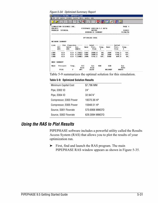
Figure 5-34: Optimized Summary Report

Table 5-9 summarizes the optimal solution for this simulation.

Using the RAS to Plot ResultsPIPEPHASE software includes a powerful utility called the Results Access System (RAS) that allows you to plot the results of your optimization run.

➤ First, find and launch the RAS program. The main PIPEPHASE RAS window appears as shown in Figure 5-35.

Table 5-9: Optimized Solution Results

Minimum Capital Cost $7,796 MM

Pipe, E002 ID 24”

Pipe, E004 ID 32.9474”

Compressor, E003 Power 18370.36 hP

Compressor, E005 Power 15948.51 hP

Source, S001 Flowrate 570.6906 MMCFD

Source, S002 Flowrate 629.3094 MMCFD


Figure 5-35: PIPEPHASE RAS Window

➤ Next, select the File/New menu option.

➤ Select the OPTEXAM1.RAS database file.

➤ Click the View/Edit button beside the Plot Report drop-down list box to define your plot. This brings up the RAS Plot Options window.

➤ Click the Add button to bring up the RAS Plot Data Options window.

➤ Next you must plot the pressure along link L003 (from junction J004 to sink D003) for the base case and the optimized case.

By default, the Initial Case option is selected in the Simulation drop-down list box.

➤ Select L003 from the Link Name drop-down list box.

➤ Check the All Devices in the Link check box.

By default, PIPEPHASE RAS will select Pressure as the State Variable to plot on the y-axis.

➤ Click the Add Selection button to add this to the list of variables to plot.

➤ Repeat the above steps for link L003 for the Optimized Case.

➤ Click the Done button to return to the RAS Plot Options window.

5-32 Tutorial

➤ Fill in the Title, X-Axis Label, and Y-Axis Label fields as shown in Figure 5-36.

Figure 5-36: RAS Plot Options Window

➤ Click the View button to view the plot shown in Figure 5-37.

Figure 5-37: RAS Plot

You can save this plot or export the data as a comma-delimited or tab-delimited ASCII file using the File menu options on the Plot window.


➤ Select File/Close to close the Plot window.

➤ Click OK on the RAS Plot Options window to return to the main RAS window.

Generate and View Excel ReportPIPEPHASE software has extended its capability to generate and view reports on the results of an optimization run in an Excel format.

Procedure to invoke Excel report has been listed below:

➤ Select Generate Excel Report.. option in View Output Menu or click Excel Reports icon in the toolbar to generate an Excel report for a currently opened simulation. Excel Reports dialog box (see figure 6-38) will pop up on selecting this option.

➤ In the Excel Reports dialog box, different types of Summary and Line reports available to be generated will be listed. You can observe some of the options have been already selected. The selected options are called Set default ‘Print Options’.


Figure 5-38: Excel Reports

5-34 Tutorial

➤ Click Run Current Network to execute the options checked under Run Options. This will generate Excel Reports for the simulation, which is currently opened.

Including Operating CostsThe analysis done in the first half of this tutorial is based on capital expenditures alone. Over the lifetime of a pipeline, the operating costs, primarily in terms of fuel consumed in running the compressors, are significant. Table 5-10 shows the compressor operating costs.

First, change the objective function to include these new costs and rerun the optimization.

➤ Click the button on the toolbar or select the General/Optimization Data menu option. This brings up the Network Optimization Data window.

➤ Click the Objective Parameters button to bring up the Network Optimization Objective Parameters window.

➤ Highlight the Compressor E005 Available Power parameter, then click the Edit button.

➤ Change the value of the Correlation Coefficient from 4.660e-003 to 6.600e-004 as shown in Figure 5-39.

Note: Uncheck the Run Simulation option under Run Options, if you have already run the simulation through Run Simulation and View Results dialog box. Excel Reports dialog box can be viewed by clicking Excel button present in Run Simulation and View Results dialog box.

Table 5-10: Compressor Operating Costs

Compressor Cost/1000hP $0.44 MM/year

Over the lifetime of the pipeline system (10 years), the total cost is therefore:

Total = Operating Costs + Capital CostCosts (MMD) = (4.0E-4*10*wCompr 1 + 4.0E-4*10*wCompr 2) + (140*IDPipe 1 +126*IDPipe 2 + 4.66E-3*wCompr 1 + 4.66E-3*wCompr 2)


Figure 5-39: Define Objective Parameter Window

➤ Click the OK button to return to the Network Optimization Objective Parameters window.

➤ Repeat for the Correlation Coefficient for the Compressor E003 Available Power parameter.

➤ Click the OK button until you return to the main PIPEPHASE window.

➤ Then run the modified problem by clicking the Run on the toolbar or on the File/Run menu option.

➤ Then click the Run button on the Run Simulation and View Results window.

➤ Select the Optimized Summary option from the Reports drop-down list box.

Table 5-11 compares the optimal solution for the modified problem to that of the original problem. The operating costs involved in running the pipeline system for 10 years based on the original solution are also included.


Run #2 Run #1

Minimum Total Cost $7,964 MM $7,933.8 MM MM

Capital Cost $7,574 MM $7,796 MM

Operating Cost $389.9 MM $137.3 MM

Pipe, E002 ID 24” 24”

Pipe, E004 ID 32.04 32.9474”

Compressor, E003 Power 47,476 hP 18366.76 HP

Compressor, E005 Power 50,000 hP 15949.10 HP

5-36 Tutorial

The results of these two runs show that by taking the operating costs into consideration:

■ Smaller compressors on both sections of pipeline are needed.

■ For an increased capital expenditure of $222MM in laying down slightly larger pipes on Link L003, operating costs over the lifetime of the pipeline are reduced nearly 65% from $389.9 MM to $137.3 MM.

■ Overall costs are reduced 0.3% from $7,964 MM to $7,933 MM.

Source, S001 Flowrate 565.32 MMSCFD 570.6906 MMCFD

Source, S002 Flowrate 634.67 MMSCFD 629.3094 MMCFD

1Operating cost = 47.476*0.4*10+50*0.4*10=$389 MM


Run #2 Run #1


5-38 Tutorial

Index

A

Additional Component Capabilities 4-17

Additional Thermodynamic Capabilities 4-20

Assay Curve 4-16

C

Compiler requirements 1-2

Custom (full) installationoption 2-1

D

Default installationdisk space requirement 1-3

Default installation directory 2-5

Defaults 4-13

DefiningFluid Properties 4-14Properties for Compositional Fluids 4-14Properties for Mixed Compositional/ Non-Compositional Fluids 4-24Properties for Non-compositional Fluids

Liquid 4-21

Defining Properties for Non-compositional Fluids 4-21

Disk space requirementsPIPEPHASE 1-3

Documentation 1-viiiprinted material 1-1

E

Exiting PIPEPHASE 4-2

F

FLEXlm 2-4, 2-6

FLEXlm9.5 2-4, 2-6

Full installationdisk space requirement 1-3

G

Gaslift and Sphering 4-10

Generating and Using Tables of Properties 4-25

H

Hardware requirements 1-2

Heat Transfer Calculations 4-41

Help, online 1-viii

I

Installationtroubleshooting 3-1

installation 2-1

Installation options 2-1

InstallingPIPEPHASE 2-1standalone 2-2

Installing a Standalone Version 2-2

L

Library Components 4-15

M

Media 1-1

PIPEPHASE 9.5 Getting Started Guide I-1

N

Nodal Analysis 4-50

Nominal Diameter 4-34

Non-library Components 4-15

O

Onlinedocumentation 1-viiihelp 1-viii

Operating system requirements 1-2

P

Petroleum Pseudocomponents 4-15

Pipe Schedule 4-34

PIPEPHASECase Studies 4-48Changing Window Size 4-3Color Coding Cues 4-3disk space requirements 1-3documentation 1-1Equipment Items 4-38Global Settings 4-11hardware/software requirements 1-2installing 2-1, 2-8Main Window Components 4-2media 1-1Menu Options 4-4package contents 1-1reviewing the results 2-8testing the installation 2-7Toolbar Buttons 4-5Units of Measurement 4-11

Piping Structure 4-10

Pressure Drop in Completions 4-36

Pressure Drop in Fittings 4-36

Pressure Drop in Flow Devices 4-33

Printout Options 4-12

PRO/IIicons 2-5

Production Planning 4-43

Properties for Non-compositional FluidsBlackoil 4-23

Gas 4-22Gas Condensate 4-23Liquid 4-21Steam 4-22

R

RelationshipsReservoirs and Inflow Performance 4-42

Results 2-8

S

SecurityElan 1-3

Security optionsselecting for PRO/II 2-4, 2-6

Software requirements 1-2

Sources 4-25

Sphering or Pigging 4-42

Starting PIPEPHASE 4-1

Structure of Network Systems 4-26

Subsurface Networks and Multiple Completion Modeling 4-45

Support 1-x

T

Technical support centers 1-xi

Testing PIPEPHASE 2-7

Thermodynamic Properties and Phase Separation 4-17

Time-stepping 4-43

Transport Properties 4-19

Troubleshooting 3-1

Troubleshooting installation problems 3-1

Typical (default) installationoption 2-1

U

UninstallingPIPEPHASE 2-8

User-added subroutinesdisk space requirement 1-3

Index I-2

installation option 2-1installing 2-5

Using PIPEPHASE 4-8

V

Viewing and Plotting Results 5-30

PIPEPHASE 9.5 Getting Started Guide I-3

PIPEPHASE_9.5_Getting_Started_Guide.pdf

Documents

testing pipephase software

exiting pipephase software

pipephase window

pipephase user

software requirements

token security

invensys logo

flexnet security