Pipelining Saturated Accumulation

Appearing in IEEE International Conference on Field-Programmable Technology (FPT 2005), December 11–14, 2005

Pipelining Saturated Accumulation

Karl Papadantonakis, Nachiket Kapre, Stephanie Chan, and Andre DeHonDepartment of Computer ScienceCalifornia Institute of Technology

Pasadena, CA [email protected]

Abstract

Aggressive pipelining allows FPGAs to achievehigh throughput on many Digital Signal Process-ing applications. However, cyclic data dependenciesin the computation can limit pipelining and reducethe efficiency and speed of an FPGA implementa-tion. Saturated accumulation is an important exam-ple where such a cycle limits the throughput of signalprocessing applications. We show how to reformu-late saturated addition as an associative operationso that we can use a parallel-prefix calculation toperform saturated accumulation at any data rate sup-ported by the device. This allows us, for example, todesign a 16-bit saturated accumulator which can op-erate at 280MHz on a Xilinx Spartan-3 (XC3S-5000-4), the maximum frequency supported by the compo-nent’s DCM.

1. Introduction

FPGAs have high computational density (e.g. theyoffer a large number of bit operations per unit space-time) when they can be run at high throughput (e.g.[1]). To achieve this high density, we must aggres-sively pipeline designs exploiting the large number ofregisters in FPGA architectures. In the extreme, wepipeline designs so that only a single LookUp-Table(LUT) delay and local interconnect is in the latencypath between registers (e.g. [2]). Pipelined at thislevel, conventional FPGAs should be able to run withclock rates in the hundreds of megahertz.

For acyclic designs (feed forward dataflow), it isalways possible to perform this pipelining. It may benecessary to pipeline the interconnect (e.g. [3, 4]), butthe transformation can be performed and automated.

However, when a design has a cycle which has alarge latency but only a few registers in the path, wecannot immediately pipeline to this limit. No legalretiming [5] will allow us to reduce the ratio betweenthe total cycle logic delay (e.g. number of LUTs inthe path) and the total registers in the cycle. This of-ten prevents us from pipelining the design all the way

down to the single LUT plus local interconnect leveland consequently prevents us from operating at peakthroughput to use the device efficiently. We can usethe device efficiently by interleaving parallel prob-lems in C-slow fashion (e.g. [5, 6]), but the through-put delivered to a single data stream is limited. In aspatial pipeline of streaming operators, the through-put of the slowest operator will serve as a bottleneck,forcing all operators to run at the slower through-put, preventing us from achieving high computationaldensity.

Saturated accumulation (Section 2.1) is a commonsignal processing operation with a cyclic dependencewhich prevents aggressive pipelining. As such, itcan serve as the rate limiter in streaming applications(Section 2.2). While non-saturated accumulation isamenable to associative transformations (e.g. delayedaddition [7] or block associative reduce trees (Sec-tion 2.4)), the non-associativity of the basic saturatedaddition operation prevents these direct transforma-tions.

In this paper we show how to transform sat-urated accumulation into an associative operation(Section 3). Once transformed, we use a parallel-prefix computation to avoid the apparent cyclic de-pendencies in the original operation (Section 2.5). Asa concrete demonstration of this technique, we showhow to accelerate a 16-bit accumulation on a XilinxSpartan-3 (X3CS-5000-4) [8] from a cycle time of11.3ns to a cycle time below 3.57ns (Section 5). Thetechniques introduced here are general and allow usto pipeline saturated accumulations to any throughputwhich the device can support.

2. Background

2.1. Saturated Accumulation

Efficient implementations of arithmetic on realcomputing devices with finite hardware must dealwith the fact that integer addition is not closed overany non-trivial finite subset of the integers. Somecomputer arithmetic systems deal with this by us-ing addition modulo a power of two (e.g. addition

c© 2005 IEEE 1

input (xi) 0 50 100 100 11 -2modulo sum 0 50 150 250 5 3

(mod 256)satsum (yi) 0 50 150 250 255 253

(maxval=256)

Table 1. Accumulation Example

modulo 232 is provided by most microprocessors).However, for many applications, modulo addition hasbad effects, creating aliasing between large numberswhich overflow to small numbers and small numbers.Consequently, one is driven to use a large modulus(a large number of bits) in an attempt to avoid thisaliasing problem.

An alternative to using wide datapaths to avoidaliasing is to define saturating arithmetic. Instead ofwrapping the arithmetic result in modulo fashion, thearithmetic sets bounds and clips sums which go outof bounds to the bounding values. That is, we definea saturated addition as:

SA(a,b,minval,maxval) {tmp=a+b; // tmp can hold sum

// without wrappingif (tmp>maxval) return(maxval);elseif (tmp<minval) return(minval);else return(tmp)

}

Since large sums cannot wrap to small values whenthe precision limit is reached, this admits economi-cal implementations which use modest precision formany signal processing applications.

A saturated accumulator takes a stream of inputvalues xi and produces a stream of output values yi:

yi = SA(yi−1, xi,minval,maxval) (1)

Table 1 gives an example showing the difference be-tween modulo and saturated accumulation.

2.2. Example: ADPCM

The decoder in the Adaptive Differential Pulse-Compression Modulation (ADPCM) application inthe mediabench benchmark suite [9] provides aconcrete example where saturated accumulation isthe bottleneck limiting application throughput. Fig-ure 1 shows the dataflow path for the ADPCM de-coder. The only cycles which exist in the dataflowpath are the two saturated accumulators. Note that wecan accommodate pipeline delays at the beginning ofthe datapath, at the end of the datapath, and even inthe middle between the two saturated accumulators(annotated in Figure 1) without changing the seman-tics of the decoder operation. As with any pipeliningoperation, such pipelining will change the number ofcycles of latency between the input (delta) and theoutput (valpred).

Previous attempts to accelerate the mediabenchapplications for spatial (hardware or FPGA) imple-mentation have achieved only modest acceleration onADPCM (e.g. [10]). This has led people to char-acterize ADPCM as a serial application. With thenew transformations introduced here, we show howwe can parallelize this application.

2.3. Associativity

Both infinite precision integer addition and mod-ulo addition are associative. That is: (A + B) + C =A + (B + C). However, saturated addition is not as-sociative. For example, consider: 250+100-11

infinite precision arithmetic:(250+100)-11 = 350-11 = 339250+(100-11) = 250+89 = 339

modulo 256 arithmetic:(250+100)-11 = 94-11 = 83250+(100-11) = 250+89 = 83

saturated addition (max=255):(250+100)-11 = 255-11 = 244250+(100-11) = 250+89 = 255

Consequently, we have more freedom in implement-ing infinite precision or modulo addition than we dowhen implementing saturating addition.

2.4. Associative Reduce

When associativity holds, we can exploit the asso-ciative property to reshape the computation to allowpipelining. Consider a modulo-addition accumulator:

yi = yi−1 + xi (2)

Unrolling the accumulation sum, we can write:

yi = ((yi−3 + xi−2) + xi−1) + xi (3)

Exploiting associativity we can rewrite this as:

yi = ((yi−3 + xi−2) + (xi−1 + xi)) (4)

Whereas the original sum had a series delay of 3adders, the re-associated sum has a series delay of2 adders. In general, we can unroll this accumulationN − 1 times and reduce the computation depth fromN − 1 to log2(N) adders.

With this reassociation, the delay of the additiontree grows as log(N) while the number of clock sam-ple cycles grows as N . The unrolled cycle allows usto add registers to the cycle faster (N ) than we adddelays (log(N)). Consequently, we can select N suf-ficiently large to allow arbitrary retiming of the accu-mulation.

2.5. Parallel-Prefix Tree

In Section 2.4, we noted we could compute the fi-nal sum of N values in O(log(N)) time using O(N)

2

indexTable

min=0 max=88

sata

dd

saturatedaccumulator

stepsize Table psuedo

multiply

sata

dd

saturatedaccumulator

min=−32768 max=32767

(add pipelining here without changing semantics)

delta

index step

valpred

(4b sample)

(16b output)

(registers) (registers)

Figure 1. Dataflow for ADPCM Decode

S[0,1] S[2,3] S[4,5] S[6,7] S[8,9] S[10,11] S[12,13] S[14,15]

S[0,3] S[4,7]

S[0,7]

S[0,5]

S[0,2] S[0,4] S[0,6] S[0,8]

S[8,11] S[12,15]

S[8,15]

S[0,15]

S[0,11]

S[0,13] S[0,9]

S[0,10] S[0,12] S[0,14]

x[0] x[1] x[2] x[3] x[4] x[5] x[6] x[7] x[8] x[9] x[10] x[11] x[12] x[13] x[14] x[15]

y[0]

+ + + + + + + + + + + + + + + +

y[1] y[2] y[3] y[4] y[5] y[6] y[7] y[8] y[9] y[10] y[11] y[12] y[13] y[14] y[15] y[16]

k=2

k=3

k=4

k=1 associative reduce treeprefix tree

Figure 2. 16-input Parallel-Prefix Tree

adders. With only a constant factor more hardware,we can actually compute all N intermediate outputs:yi, yi−1, . . . y(i−(N−1)) (e.g. [11]).

We do this by computing and combiningpartial sums of the form S[s, t] which repre-sents the sum: xs + xs+1 + . . . xt. When webuild the associative reduce tree, at each levelk, we are combining S[(2j) 2k, (2j + 1) 2k−1]and S[(2j + 1) 2k, 2 (j + 1) 2k−1] to computeS[(2j) 2k, 2 (j + 1) 2k−1] (See Figure 2). Conse-quently, we eventually compute prefix spans from0 to 2k-1 (the j = 0 case), but do not eventuallycompute the other prefixes. The observation to makeis that we can combine the S[0, 2k−1] prefixes withthe S[2k0 , 2k0+2k1−1] spans (k1 < k0) to computethe intermediate results. To compute the full prefixsequence (S[0, 1],S[0, 2], . . .S[0, N−1]), we add asecond (reverse) tree to compute these intermediateprefixes. At each tree level where we have a composeunit in the forward, associative reduce tree, we add(at most) one more, matching, compose unit inthis reverse tree. The reverse, or prefix, tree is nolarger than the reduce tree; consequently, the entireparallel-prefix tree is at most twice the size of theassociative reduce tree. Figure 2 shows a width16 parallel-prefix tree for saturated accumulation.For a more tutorial development of parallel-prefixcomputations see [11, 12].

2.6. Prior Work

Balzola et al. attacked the problem of saturatingaccumulation at the bit level [13]. They observed theycould reduce the logic in the critical cycle by comput-ing partial sums for the possible saturation cases andusing a fast, bit-level multiplexing network to rapidlyselect and compose the correct final sums. They wereable to reduce the cycle so it only contained a singlecarry-propagate adder and some bit-level multiplex-ing. For custom designs, this minimal cycle may besufficiently small to provide the desired throughput.In contrast, our solution makes the saturating opera-tions associative. Our solution may be more impor-tant for FPGA designs where the designer has lessfreedom to implement a fast adder and must pay forprogrammable interconnect delays for the bit-levelcontrol.

3. Associative Reformulation of SaturatedAccumulation

Unrolling the computation we need to perform forsaturated additions, we get a chain of saturated addi-tions (SA), such as:

x[i]

SA SA SA SAy[i]y[i−1]y[i−2]y[i−3]y[i−4]

x[i−

1]

x[i−

2]

x[i−

3]m

axva

lm

inva

l

max

val

min

val

max

val

min

val

max

val

min

val

We can express SA (Section 2.1) as a function usingmax and min:

SA(y, x,minval,maxval) (5)= min(max((y + x),minval),maxval)

The saturated accumulation is repeated application ofthis function. We seek to express this function in sucha way that repeated application is function compo-sition. This allows us to exploit the associativity offunction composition [14] so we can compute satu-rated accumulation using a parallel-prefix tree (Sec-tion 2.5)

Technically, function composition does not applydirectly to the formula for SA shown in Equation 5

3

because that formula is a function of four inputs (hav-ing just one output, y). Fortunately, only the depen-dence on y is critical at each SA-application step; theother inputs are not critical, because it is easy to guar-antee that they are available in time, regardless of ouralgorithm. To understand repeated application of theSA function, therefore, we express SA in an alternateform in which y is a function of a single input and theother “inputs” (x, minval, and maxval) are func-tion parameters:

SA[x,m,M ](y) def= SA(y, x, m,M) (6)

We define SA[i] as the ith application of this func-tion, which has x = x[i], m = minval, andM = maxval:

SA[i] def= SA[x[i],minval,maxval] (7)

This definition allows us to view the computation asfunction composition. For example:

y[i] = SA[i] ◦ SA[i−1]◦ SA[i−2] ◦ SA[i−3](y[i−4]) (8)

x[i]

SA SA SA SAy[i]y[i−1]y[i−2]y[i−3]y[i−4]

x[i−

1]

x[i−

2]

x[i−

3]m

axva

lm

inva

l

SA[i−3] SA[i−2] SA[i−1] SA[i]

max

val

min

val

max

val

min

val

max

val

min

val

3.1. Composing the SA functions

To reduce the critical latency implied by Equa-tion 8, we first combine successive nonoverlappingadjacent pairs of operations (just as we did with ordi-nary addition in Equation 4). For example:

y[i] = ((SA[i] ◦ SA[i−1])◦ (SA[i−2] ◦ SA[i−3])) (y[i−4])

To make this practical, we need an efficient way tocompute each adjacent pair of operations in one step:

SA[i−1, i] def= SA[i] ◦ SA[i−1] (9)

SA SAy[i−3]y[i−4]

x[i−

2]

x[i−

3]m

axva

lm

inva

l

SA[i−3] SA[i−2]

max

val

min

val

SA[i−1,i]

y[i−2]

x[i]

SAy[i]y[i−1]

x[i−

1]

SA[i−1] SA[i]

max

val

min

val

max

val

min

val

SA

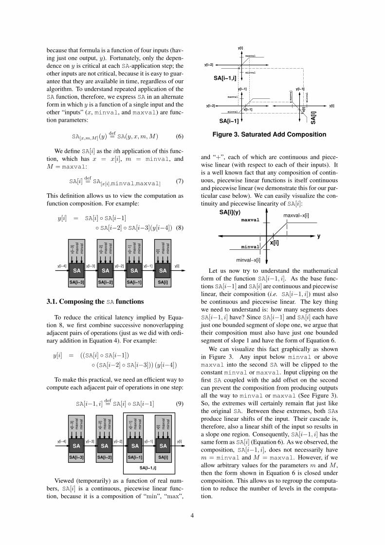
Viewed (temporarily) as a function of real num-bers, SA[i] is a continuous, piecewise linear func-tion, because it is a composition of “min”, “max”,

y[i−2]

y[i−1]

y[i]

y[i−1]

minval

maxval

minval

maxval

SA[i−1] SA

[i]

x[i−1] x[i]

y[i]

y[i−2]

maxval

minval

SA[i−1,i]

Figure 3. Saturated Add Composition

and “+”, each of which are continuous and piece-wise linear (with respect to each of their inputs). Itis a well known fact that any composition of contin-uous, piecewise linear functions is itself continuousand piecewise linear (we demonstrate this for our par-ticular case below). We can easily visualize the con-tinuity and piecewise linearity of SA[i]:

minval

maxval

x[i]

minval−x[i]

maxval−x[i]

y

SA[i](y)

Let us now try to understand the mathematicalform of the function SA[i−1, i]. As the base func-tions SA[i−1] and SA[i] are continuous and piecewiselinear, their composition (i.e. SA[i−1, i]) must alsobe continuous and piecewise linear. The key thingwe need to understand is: how many segments doesSA[i−1, i] have? Since SA[i−1] and SA[i] each havejust one bounded segment of slope one, we argue thattheir composition must also have just one boundedsegment of slope 1 and have the form of Equation 6.

We can visualize this fact graphically as shownin Figure 3. Any input below minval or abovemaxval into the second SA will be clipped to theconstant minval or maxval. Input clipping on thefirst SA coupled with the add offset on the secondcan prevent the composition from producing outputsall the way to minval or maxval (See Figure 3).So, the extremes will certainly remain flat just likethe original SA. Between these extremes, both SAsproduce linear shifts of the input. Their cascade is,therefore, also a linear shift of the input so results ina slope one region. Consequently, SA[i−1, i] has thesame form as SA[i] (Equation 6). As we observed, thecomposition, SA[i−1, i], does not necessarily havem = minval and M = maxval. However, if weallow arbitrary values for the parameters m and M ,then the form shown in Equation 6 is closed undercomposition. This allows us to regroup the computa-tion to reduce the number of levels in the computa-tion.

4

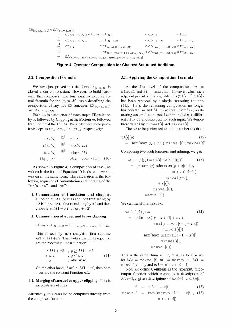
SA[x2,m2,M2] ◦ SA[x1,m1,M1]

= ctM2 ◦ cbm2 ◦ trx2 ◦ ctM1 ◦ cbm1 ◦ trx1I= ctM2 ◦ cbm2 ◦ ctM1+x2 ◦ cbm1+x2 ◦ trx1+x2II= ctM2 ◦ ctmax(M1+x2,m2) ◦ cbmax(m1+x2,m2) ◦ trx1+x2III= ctmin(max(M1+x2,m2),M2) ◦ cbmax(m1+x2,m2) ◦ trx1+x2

= SA[x1+x2,max(m1+x2,m2),min(max(M1+x2,m2),M2)]

Figure 4. Operator Composition for Chained Saturated Additions

3.2. Composition Formula

We have just proved that the form SA[x,m,M ] isclosed under composition. However, to build hard-ware that composes these functions, we need an ac-tual formula for the [x, m,M ] tuple describing thecomposition of any two SA functions SA[x1,m1,M1]

and SA[x2,m2,M2].Each SA is a sequence of three steps: TRanslation

by x, followed by Clipping at the Bottom m, followedby Clipping at the Top M . We write these three prim-itive steps as trx, cbm, and ctM , respectively:

trx(y) def= y + x

cbm(y) def= max(y, m)

ctM (y) def= min(y, M)SA[x,m,M ] = ctM ◦ cbm ◦ trx (10)

As shown in Figure 4, a composition of two SAswritten in the form of Equation 10 leads to a new SAwritten in the same form. The calculation is the fol-lowing sequence of commutation and merging of the“tr”s, “cb”s, and “ct”s:

I. Commutation of translation and clipping.Clipping at M1 (or m1) and then translating byx2 is the same as first translating by x2 and thenclipping at M1 + x2 (or m1 + x2).

II. Commutation of upper and lower clipping.

cbm2 ◦ ctM1+x2 = ctmax(M1+x2,m2) ◦ cbm2

This is seen by case analysis: first supposem2 ≤ M1+x2. Then both sides of the equationare the piecewise linear function{

M1 + x2 , y ≥ M1 + x2m2 , y ≤ m2y , otherwise.

(11)

On the other hand, if m2 > M1 + x2, then bothsides are the constant function m2.

III. Merging of successive upper clipping. This isassociativity of min.

Alternately, this can also be computed directly fromthe composed function.

3.3. Applying the Composition Formula

At the first level of the computation, m =minval and M = maxval. However, after eachadjacent pair of saturating additions (SA[i−1], SA[i])has been replaced by a single saturating addition(SA[i−1, i]), the remaining computation no longerhas constant m and M . In general, therefore, a sat-urating accumulation specification includes a differ-ent minval and maxval for each input. We denotethese values by minval[i] and maxval[i].

The SA to be performed on input number i is then:

SA[i](y) (12)= min(max((y + x[i]),minval[i]),maxval[i])

Composing two such functions and inlining, we get:

SA[i−1, i](y) = SA[i](SA[i−1](y)) (13)= min(max((min(max((y + x[i−1]),

minval[i−1]),maxval[i−1])

+ x[i]),minval[i]),

maxval[i])

We can transform this into:

SA[i−1, i](y) = (14)= min(max((y + x[i−1] + x[i]),

max((minval[i−1] + x[i]),minval[i])),

min(max((maxval[i−1] + x[i]),minval[i]),

maxval[i]))

This is the same thing as Figure 4, as long as welet M2 = maxval[i], m2 = minval[i], M1 =maxval[i− 1], and m2 = minval[i− 1].

Now we define Compose as the six-input, three-output function which computes a description ofSA[i−1, i] given descriptions of SA[i−1] and SA[i]:

x′ = x[i−1] + x[i] (15)minval′ = max((minval[i−1] + x[i]), (16)

minval[i])

5

SA

x[i−

1]

x[i]x[i−

2]

x[i−

3]

x[i]

SA SA SA SAy[i]y[i−1]y[i−2]y[i−3]y[i−4]

x[i−

1]

x[i−

2]

x[i−

3]m

axva

lm

inva

l

max

val

min

val

max

val

min

val

max

val

min

val

SA[i−3] SA[i−2] SA[i−1] SA[i]

max

val[i

−3]

min

val[i

−3]

max

val[i

−2]

min

val[i

−2]

max

val[i

−1]

min

val[i

−1]

max

val[i

]m

inva

l[i]

x[i−3,i] maxval[i−3,i] minval[i−3,i]

y[i−4] y[i]SA

SA[i−3,i]

Compose Compose

x[i−3,i−2] x[i−1,i]minval[i−3,i−2]maxval[i−3,i−2] maxval[i−1,i] minval[i−1,i]

Compose

Figure 5. Composition of SA[(i− 3), i]

maxval′ = min(max((maxval[i−1] + x[i]),minval[i]), (17)

maxval[i])

This gives us:

SA[i−1, i](y) (18)= min(max(y + x′),minval′),maxval′)

This allows us to compute SA[i, j](y) as shown inFigure 5. One can note this is a very similar strategyto the combination of “propagates” and “generates”in carry-lookahead addition (e.g. [12]).

3.4. Wordsize of Intermediate Values

The preceding correctness arguments rely on theassumption that intermediate values (i.e. all valuesever computed by the Compose function) are math-ematical integers; i.e., they never overflow. For acomputation of depth k, at most 2k numbers are everadded, so intermediate values can be represented inW+k bits if the inputs are represented in W bits.While this gives us an asymptotically tight result, wecan actually do all computation with W+2 bits (2’scomplement representation) regardless of k.

First, notice that maxval′ is always betweenminval[i] and maxval[i]. The same is not trueabout minval′, until we make a slight modificationto Equation 16; we redefine minval′ as follows:

minval′ = min(max((minval[i−1] + x[i]),minval[i]), (19)

maxval[i])

+

max

A B

SA min

maxvalminval

Figure 6. Saturated Adder

+ +

maxSA

+

maxSA

x[i]

Compose

min min

x[i−1]

x[i−1,i] maxval[i−1,i] minval[i−1,i]

maxval[i−1] minval[i−1] maxval[i] minval[i]

w−bit w−bit

(w+2)−bit

Figure 7. Composition Unit for Two Sat-urated Additions

This change does not affect the result because it onlycauses a decrease in minval′ when it is greaterthan maxval′. While it is more work to do theextra operation, it is only a constant increase, andthis extra work is done anyway if the hardware formaxval′ is reused for minval′ (See Section 4).With this change, the interval [minval′,maxval′]is contained in the interval [minval[i],maxval[i]],so none of these quantities ever requires more than Wbits to represent.

If we use (W+2)-bit datapaths for computing x′,x′ can overflow in the tree, as the “x”s are neverclipped. We argue that this does not matter. Wecan show that whenever x′ overflows, its value is ig-nored, because a constant function is represented (i.e.minval′ = maxval′). Furthermore, we need notkeep track of when an overflow has occured, since ifminval = maxval, then minval′ = maxval′ atall subsequent levels of the computation, as this prop-erty is maintained by Equations 17 and 19.

4. Putting it Together

Knowing how to compute SA[i, i−1] from the pa-rameters for SA[i] and SA[i−1], we can unroll thecomputation to match the delay through the saturatedaddition and create a suitable parallel-prefix compu-tation (similar to Sections 2.4 and 2.5). From the pre-vious section, we know the core computation for thecomposer is, itself, saturated addition (Eqs. 15, 17,and 19). Using the saturated adder shown in Figure 6,we build the composer as shown in Figure 7.

6

SA

Compose

Compose

Compose

Compose

SASASA

slowf

ffast

ffast

TwoPipelineStages

0

(register)

Figure 8. N = 4 Parallel-Prefix Saturat-ing Accumulator

5. Implementation

We implemented the parallel-prefix saturated ac-cumulator in VHDL to demonstrate functionality andget performance and area estimates. We used Model-sim 5.8 to verify the functionality of the design andSynplify Pro 7.7 and Xilinx ISE 6.1.02i to map ourdesign onto the target device. We did not provideany area constraints and let the tools automaticallyplace and route the design using just the timing con-straints. We chose a Spartan-3 XC3S-5000-4 as ourtarget device. The DCMs on the Spartan-3 (speedgrade -4 part) support a maximum frequency of 280Mhz (3.57ns cycle), so we picked this maximum sup-ported frequency as our performance target.

Design Details The parallel-prefix saturating accu-mulator consists of a parallel-prefix computation treesandwiched between a serializer and deserializer asshown in Figure 8. Consequently, we decompose thedesign into two clock domains. The higher frequencyclock domain pushes data into the slower frequencydomain of the parallel-prefix tree. The parallel-prefixtree runs at a proportionally slower rate to accomo-date the saturating adders shown in Figures 6 and 7.Minimizing the delays in the tree requires us to com-pute each compose in two pipeline stages. Finally,we clock the result of the prefix computation into thehigher frequency clock domain in parallel then seri-ally shift out the data at the higher clock frequency.

It is worthwhile to note that the delay through thecomposers is actually irrelevant to the correct opera-tion of the saturated accumulation. The compositiontree adds a uniform number of clock cycle delays be-tween the x[i] shift register and the final saturated ac-cumulator. It does not add to the saturated accumula-tion feedback latency which the unrolling must cover.This is why we can safely pipeline compose stages inthe parallel-prefix tree.

Datapath Width (W ) 2 4 8 16 32Prefix-tree Width (N ) 3 3 4 4 4

Table 2. Minimum Size of Prefix Tree Re-quired to Achieve 280MHz

Area We express the area required by this design asa function of N (loop unroll factor) and W (bitwidth).Intuitively, we can quickly see that the area requiredfor the prefix tree is roughly 5 2

3N times the area ofa single saturated adder. The initial reduce tree hasroughly N compose units, as does the final prefixtree. Each compose unit has two W -bit saturatedadders and one (W+2)-bit regular adder, and eachadder requires roughly W/2 slices. Together, thisgives us ≈ 2 × (2× 3 + 1) NW/2 slices. Finally,we add a row of saturated adders to compute the finaloutput to get a total of 17

2 NW slices. Compared tothe base saturated adder which takes 3

2W slices, thisis a factor of 17N

3 = 5 23N .

Pipelining levels in the parallel-prefix tree roughlycosts us 2 × 3 × N registers per level times the2 log2(N) levels for a total of 12N log2(N)W reg-isters. The pair of registers for a pipe stage can fitin a single SRL16, so this should add no more than3N log2(N)W slices.

A(N,W ) ≈ 3N log2(N)W +172

NW (20)

This approximation does not count the overhead ofthe control logic in the serializer and deserializersince it is small compared to the registers. For rip-ple carry adders, N = O(W ) and this says area willscale as O

(W 2 log (W )

). If we use efficient, log-

depth adders, N = O (log(W )) and area scales asO (W log (W ) log (log (W ))).

If the size of the tree is N and the frequency of thebasic unpipelined saturating accumulator is f , thenthe system can run at a frequency f ×N . By increas-ing the size of the parallel-prefix tree, we can makethe design run arbitrarily fast, up to the maximum at-tainable speed of the device. In Table 2 we show thevalue of N (i.e. the size of the prefix tree) requiredto achieve a 3ns cycle target. We target this tightercycle time (compared to the 3.57ns DCM limit) to re-serve some headroom going into place and route forthe larger designs.

Results Table 3 shows the clock period achieved byall the designs for N = 4 after place and route. Webeat the required 3.57ns performance limit for all thecases we considered. In Table 3 we show the actualarea in SLICEs required to perform the mapping fordifferent bitwidths W . A 16-bit saturating accumu-lator requires 1065 SLICEs which constitutes around2% of the XC3S-5000. We also show that an areaoverhead of less than 25× is required to achieve this

7

DatapathWidth (W ) 2 4 8 16 32Simple Saturated AccumulatorDelay (ns) 6.2 8.1 9.1 11.3 13.4

SLICEs 10 14 24 44 84Parallel-Prefix Saturated Accumulator (N = 4)Delay (ns) 2.8 2.7 3.1 2.9 3.3

SLICEs 215 333 571 1065 2085Ratios: Parallel-Prefix/Simple

Freq. 2.2 3.0 2.9 3.6 4.1Area 22 24 24 24 25

Table 3. Accumulator Comparison

speedup over an unpipelined simple saturating accu-mulator; for N = 4, 5 2

3N ≈ 23, so this is consistentwith our intuitive prediction aboves.

6. Summary

Saturated accumulation has a loop dependencythat, naively, limits single-stream throughput and ourability to fully exploit the computational capacity ofmodern FPGAs. We show that this loop dependenceis actually avoidable by reformulating the saturatedaddition as the composition of a series of functions.We further show that this particular function compo-sition is, asymptotically, no more complex than theoriginal saturated addition operation. Function com-position is associative, so this reformulation allows usto build a parallel-prefix tree in order to compute thesaturated accumulation over several loop iterations inparallel. Consequently, we can unroll the saturatedaccumulation loop to cover the delay through the sat-urated adder. As a result, we show how to computesaturated accumulation at any data rate supported byan FPGA.

Acknowledgments

This research was funded in part by the NSF undergrant CCR-0205471. Stephanie Chan was supportedby the Marcella Bonsall SURF Fellowship. Karl Pa-padantonakis was supported by a Moore Fellowship.Scott Weber and Eylon Caspi developed early FPGAimplementations of ADPCM which helped identifythis challenge. Michael Wrighton provided VHDLcoding and CAD tool usage tips.

7. References

[1] A. DeHon, “The Density Advantage of Config-urable Computing,” IEEE Computer, vol. 33,no. 4, pp. 41–49, April 2000.

[2] B. V. Herzen, “Signal Processing at 250 MHzusing High-Performance FPGA’s,” in FPGA,February 1997, pp. 62–68.

[3] W. Tsu, K. Macy, A. Joshi, R. Huang,N. Walker, T. Tung, O. Rowhani, V. George,J. Wawrzynek, and A. DeHon, “HSRA: High-Speed, Hierarchical Synchronous Reconfig-urable Array,” in FPGA, February 1999, pp.125–134.

[4] D. P. Singh and S. D. Brown, “The Casefor Registered Routing Switches in Field Pro-grammable Gate Arrays,” in FPGA, February2001, pp. 161–169.

[5] C. Leiserson, F. Rose, and J. Saxe, “OptimizingSynchronous Circuitry by Retiming,” in ThirdCaltech Conference On VLSI, March 1983.

[6] N. Weaver, Y. Markovskiy, Y. Patel, andJ. Wawrzynek, “Post-Placement C-slow Retim-ing for the Xilinx Virtex FPGA,” in FPGA,2003, pp. 185–194.

[7] Z. Luo and M. Martonosi, “AcceleratingPipelined Integer and Floating-Point Accumu-lations in Configurable Hardware with DelayedAddition Techniques,” IEEE Tr. on Computers,vol. 49, no. 3, pp. 208–218, March 2000.

[8] Xilinx Spartan-3 FPGA Family Data Sheet ,Xilinx, Inc., 2100 Logic Drive, San Jose, CA95124, December 2004, dS099 <http://direct.xilinx.com/bvdocs/publications/ds099.pdf>.

[9] C. Lee, M. Potkonjak, and W. H. Mangione-Smith, “MediaBench: A Tool for Evaluatingand Synthesizing Multimedia and Communica-tons Systems,” in International Symposium onMicroarchitecture, 1997, pp. 330–335.

[10] R. Barua, W. Lee, S. Amarasinghe, andA. Agarwal, “Maps: A Compiler-ManagedMemory System for Raw Machines,” in ISCA,1999.

[11] W. D. Hillis and G. L. Steele, “Data Paral-lel Algorithms,” Communications of the ACM,vol. 29, no. 12, pp. 1170–1183, December 1986.

[12] F. T. Leighton, Introduction to Parallel Algo-rithms and Architectures: Arrays, Trees, Hy-percubes. Morgan Kaufmann Publishers, Inc.,1992.

[13] P. I. Balzola, M. J. Schulte, J. Ruan, J. Gloss-ner, and E. Hokenek, “Design Alternatives forParallel Saturating Multioperand Adders,” inProceedings of the International Conference onComputer Design, September 2001, pp. 172–177.

[14] J. H. Hubbard and B. B. H. Hubbard, Vec-tor Calculus, Linear Algebra, and DifferentialForms: A Unified Approach. Prentice Hall,1999.

8

A Transforming Composed Functions

Here we show the detailed steps involved in trans-forming from Equation 13 to Equation 14.

SA[i−1, i](y) = SA[i](SA[i−1](y))= min(max((min(max((y + x[i−1]),

minval[i−1]),maxval[i−1])

+ x[i]),minval[i]),

maxval[i])

I. Commutation of translation and clippingWe can push +x[i] into the min, using:

min(a, b) + c = min((a + c), (b + c)) (21)

SA[i−1, i](y) == min(max(min(max((y + x[i−1]),

minval[i−1]) + x[i],maxval[i−1] + x[i]),

minval[i]),maxval[i])

We can push +x[i] into max, using:

max(a, b) + c = max((a + c), (b + c)) (22)

SA[i−1, i](y) == min(max(min(max((y + x[i−1] + x[i]),

(minval[i−1] + x[i])),maxval[i−1] + x[i]),

minval[i]),maxval[i])

II. Commutation of upper and lower clippingLet:

a = max ((y + x[i−1] + x[i]), (23)minval[i−1] + x[i])

b = maxval[i−1] + x[i] (24)c = minval[i] (25)

So, we have:

SA[i−1, i](y) (26)= min(max(min(a, b), c),maxval[i])

Using the identity (See Max-inside-Min Lemma inAppendix A.1):

max(min(a, b), c) = min(max(a, c),max(b, c))(27)

This can become:

SA[i−1, i](y) (28)= min(min(max(a, c),max(b, c),maxval[i])

Substituting back in the expressions a, b, c, we get:

SA[i−1, i](y) == min(min(max(max((y + x[i−1] + x[i]),

(minval[i−1] + x[i])),minval[i])

max((maxval[i−1] + x[i]),minval[i])),

maxval[i])

Using the associativity of max:

max(max(a, b), c) = max(a,max(b, c)) (29)

SA[i−1, i](y) == min(min(max((y + x[i−1] + x[i]),

max((minval[i−1] + x[i]),minval[i])),

max((maxval[i−1] + x[i]),minval[i])),

maxval[i])

III. Merging of successive upper clippingUsing the associativity of min:

min(min(a, b), c) = min(a,min(b, c)) (30)

This finally gives us:

SA[i−1, i](y) == min(max((y + x[i−1] + x[i]),

max((minval[i−1] + x[i]),minval[i])),

min(max((maxval[i−1] + x[i]),minval[i]),

maxval[i]))

A.1 Max-inside-Min Lemma

Lemma: Identity 27 is true for all a, b, c.That is, the following is an identity relation:

max(min(a, b), c) = min(max(a, c),max(b, c))

Proof:Assume a > b:We can immediately reduce the left-hand-side of

the identity to:

max(min(a, b), c) = max(b, c) (31)

9

We now turn to the right-hand-side of the identity:If c < a:

max(a, c) < max(b, c) (32)

If c ≥ a:

max(a, c) = max(b, c) (33)

So, for all c:

max(a, c) ≥ max(b, c) (34)

From this we simplify:

min(max(a, c),max(b, c)) = max(b, c) (35)

We see from Eq. 31 and 35 that both sides of theclaimed Identify 27 are equivalent under the assump-tion a > b. Note that the roles of a and b are symmet-ric. So if b < a, we have an analogous case, so theidentify will also hold.

If a = b, Eq. 31 is unchanged, and Eq. 34 stillholds, so Eq. 35 must still hold. So, the Identify alsoholds when a = b.

Therefore, we see the Identity must hold for all a,b, c. �

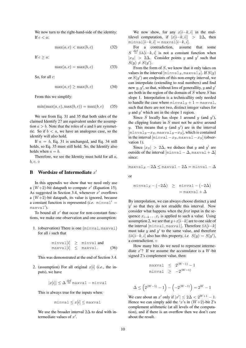
B Wordsize of Intermediate x′

In this appendix we show that we need only usea (W+2)-bit datapath to compute x′ (Equation 15).As suggested in Section 3.4, whenever x′ overflowsa (W+2)-bit datapath, its value is ignored, becausea constant function is represented (i.e. minval′ =maxval′).

To bound all x′ that occur for non-constant func-tions, we make one observation and one assumption:

1. (observation) There is one (minval,maxval)for all i such that

minval[i] ≥ minval andmaxval[i] ≤ maxval. (36)

This was demonstrated at the end of Section 3.4.

2. (assumption) For all original x[i] (i.e., the in-puts), we have

|x[i]| ≤ ∆ def= maxval− minval

This is always true for the inputs when:

minval ≤ x[i] ≤ maxval

We use the broader interval 2∆ to deal with in-termediate values of x′.

We now show, for any x[i−k, i] in the mul-tilevel computation, if |x[i−k, i]| > 2∆, thenminval[i−k, i] = maxval[i−k, i].

For a contradiction, assume that someS

def= SA[i−k, i] is not a constant function when|xS | > 2∆. Consider points y and y′ such thatS(y) 6= S(y′).

From the form of S, we know that it only takes onvalues in the interval [minvalS ,maxvalS ]. If S(y)or S(y′) are endpoints of this non-empty interval, wecan interpolate (extending to real numbers) and findnew y, y′, so that, without loss of generallity, y and y′

are both in the region of the domain of S where S hasslope 1. Interpolation is a technicallity only neededto handle the case where minvalS + 1 = maxval,such that there are not two, distinct integer values fory and y′ which are in the slope 1 region.

Since S locally has slope 1 around y (and y′),the clipping feature in S must not be active aroundy. This means that y (and y′) are in the interval[minvalS−xS ,maxvalS−xS ], which is containedin the interval [minval−xS ,maxval−xS ] (obser-vation 1).

Since |xS | > 2∆, we deduce that y and y′ areoutside of the interval [minval−∆,maxval+ ∆]since:

maxvalS − 2∆ ≤ maxval− 2∆ = minval−∆

or

minvalS − (−2∆) ≥ minval− (−2∆)= maxval+ ∆

By interpolation, we can always choose distinct y andy′ so that they do not straddle this interval. Nowconsider what happens when the first input in the se-quence xi−k . . . xi is applied to such a value. Usingassumption 2, we see that y+x[i−k] are to one side ofthe interval [minval,maxval]. Therefore SA[i−k]must take y and y′ to the same value, and thereforeSA[i−k, i] also has this property, i.e. S(y) = S(y′),a contradiction.

How many bits do we need to represent interme-diate x′? If we assume the accumulator is a W -bitsigned 2’s complement value, then:

maxval ≤ 2(W−1) − 1minval ≥ −2(W−1)

∆ ≤(2(W−1) − 1

)−

(−2(W−1)

)= 2W − 1

We care about an x′ only if |x′| ≤ 2∆ < 2W+1 − 1.Hence we can simply add the ‘x’s in (W+2)-bit 2’scomplement arithmetic (at all levels of the computa-tion), and if there is an overflow then we don’t careabout the result.

10

The 2∆ and (W+2)-bit bounds are tight: thecomputation can really have representations of non-constant functions that use all W + 2 bits. For ex-ample, suppose W = 8, with minval = −128 andmaxval = 127. Suppose x0 = x1 = −254. Thefunction SA[0, 1] is not constant, as SA[0, 1](380) =−128 while SA[0, 1](381) = −127, yet x[0, 1] =−508 requires 10 bits to represent. One might ob-serve that in this case the function is in fact con-stant because the accumulator never starts at thosevalues. However, this does not imply that minval =maxval, and while we could add extra hardware tomake this the case, it would not be worth adding thishardware just in order to save one bit. Finally, re-stricting the inputs to a smaller bound than ∆ is help-ful only in small trees, as increments up to ∆ can beachieved through a number of small increments.

Web link for this document: <http://www.cs.caltech.edu/research/ic/abstracts/sataccum_fpt2005.html>