Pipe pile setup: Database and prediction model using artificial neural network

This article appeared in a journal published by Elsevier. The attachedcopy is furnished to the author for internal non-commercial researchand education use, including for instruction at the authors institution

and sharing with colleagues.

Other uses, including reproduction and distribution, or selling orlicensing copies, or posting to personal, institutional or third party

websites are prohibited.

In most cases authors are permitted to post their version of thearticle (e.g. in Word or Tex form) to their personal website orinstitutional repository. Authors requiring further information

regarding Elsevier’s archiving and manuscript policies areencouraged to visit:

http://www.elsevier.com/authorsrights

Author's personal copy

Pipe pile setup: Database and prediction model using artificialneural network

Bashar Tarawnehn

Civil Engineering Department, The University of Jordan, Amman 11942, Jordan

Received 31 August 2012; received in revised form 14 April 2013; accepted 22 May 2013Available online 25 July 2013

Abstract

Over the last few years, artificial neural networks (ANNs) have been applied to many geotechnical engineering problems with some degree ofsuccess. With respect to the design of pile foundations, the ability to accurately predict pile setup may lead to more economical pile design,resulting in a reduction in pile length, pile section, and size of driving equipment. In this paper, an ANN model was developed for predicting pipepile setup using 104 data points, obtained from the published literature and the author's own files. In addition, the paper discusses the choice ofinput and internal network parameters which were examined to obtain the optimum ANN model.Finally, the paper compares the predictions obtained by the ANN with those given by a number of empirical formulas. It is demonstrated that

the ANN model satisfactorily predicts the measured pipe pile setup and significantly outperforms the examined empirical formulas.& 2013 The Japanese Geotechnical Society. Production and hosting by Elsevier B.V. All rights reserved.

Keywords: Pile foundation; Pile setup; Artificial neural networks

1. Introduction

Piles are relatively long and generally slender structural founda-tion members that transmit superstructure loads to deep soil layers.Piles usually serve as foundations when soil conditions are notsuitable for the use of shallow foundations. Moreover, piles haveother applications in deep excavations and in slope stability. Theultimate axial load carrying capacity of the pile is composed of theend-bearing capacity of the pile and the shaft friction capacity.

Driving a pile into the ground leads to disturbance anddisplacement of the soil surrounding the pile. As the soilrecovers from the driving disturbance, a time-dependent increase

in pile capacity regularly occurs. This phenomenon is referred toas “setup” by geotechnical engineers. A significant increase inpile capacity could occur due to this phenomenon. Consideringpile setup in the axial load capacity of driven pile may lead tomore economical pile design, leading to reduction in pile length,pile section, and size of driving equipments. Two mechanismshave been claimed to explain the setup phenomenon:

1. The dissipation of excess pore water pressure for someperiod of time after driving the piles. This is generated dueto soil remolding/disturbance during pile driving. Theassociated increase in lateral effective stress with increasingtime gives rise to an increase in shear strength and thus theaxial capacity of the pile. Obviously the duration of thisreconsolidation depends on the permeability of the soil. Itranges from days in coarse-grained soils to months or yearsin fine-grained soils (Yan and Yuen, 2010).

2. The effect of soil aging: Aging refers to a time-dependentchange in soil properties at a constant effective stress. Chow

The Japanese Geotechnical Society

www.sciencedirect.comjournal homepage: www.elsevier.com/locate/sandf

Soils and Foundations

0038-0806 & 2013 The Japanese Geotechnical Society. Production and hosting by Elsevier B.V. All rights reserved.http://dx.doi.org/10.1016/j.sandf.2013.06.011

nTel.: +962 79 754 9696.E-mail address: [email protected] review under responsibility of The Japanese Geotechnical Society.

Soils and Foundations 2013;53(4):607–615

Author's personal copy

et al. (1998) showed imperceptible increases in densityduring the aging period, so the changes in behavior must beattributable to micro-structural rearrangements of the sandgrains and their contacts with time. The changes in soilproperties due to aging are unlikely to be the major factorcontrolling setup in sand.

Chow et al. (1998) suggested that the best explanation forthe marked setup effects on driven piles in non-cohesive soilsis that sand creep rather than climatic or tide-related changes inpore pressure weakens the arching mechanisms surroundingthe pile shaft, increasing horizontal stresses while also produ-cing stronger dilation effects during loading.

Axelsson (1998) showed that pile driving in sand cangenerate strong arching effects, even at significant depths,and then the arching deteriorates with time due to stressrelaxation and leads to an increase in horizontal stress on theshaft. The increase in horizontal stress due to stress relaxationcan continue for several months and is approximately linearwith the logarithm of time. The other main reason is that soilaging phenomenon with respect to piling causes the reorienta-tion of particles, leading to interlocking. In other words, bothsoil particles interlocking with the surface roughness and stressrelaxation provide an explanation of the strong setup effects ofpile in non-cohesive soils.

Ng et al. (2013a, 2013b) studied the pile setup through afield investigation on five fully instrumented steel H-pilesembedded in cohesive soils. Based on the field data collected,it was concluded that the skin friction component, not the endbearing, contributes predominantly to the setup, which can beestimated for practical purposes using soil properties, such ascoefficient of consolidation, undrained shear strength, and thestandard penetration test N-value. A new approach wasdeveloped for estimating pile setup using dynamic measure-ments and analyses in combination with measured soilproperties.

To characterize setup, geotechnical engineers are utilizingdynamic monitoring using a Pile Driving Analyzer (PDA)during initial driving and additional dynamic monitoringduring restrike testing several hours to a few weeks afterinitial driving. On projects involving a large number of drivenpiles, the savings in pile costs can significantly exceed the costof testing required to characterize setup. However, on projectsinvolving a small number of piles, the cost of testing tocharacterize setup may exceed pile installation cost savings.Therefore, on small projects, testing required to characterizesetup directly cannot be justified from an economic standpoint.

While numerous research projects are still being carried outto study the underlying mechanisms causing the pile setup,simple empirical relations are available in the literature topredict this increase in pile capacity with time (e.g. Skov andDenver, 1988; Svinkin and Skov, 2000). The relations predictthe pile capacity from the initial capacity (described as end ofdriving, EOD) and elapsed time after driving, in which twosets of model constants were suggested for clayey and sandysoil, respectively, based on limited data sets. The reliability of

adopting these model constants is questionable. Also, the formof existing empirical relations has certain weaknesses.In this paper, Artificial Neural Networks (ANNs) are used to

predict pipe piles setup. The aims of the paper are to:

� Compile pipe pile setup data from the author's files and thepublished literature.

� Develop an (ANN) model that can predict the pipepile setup.

� Study the effect of ANN geometry and some internalparameters on the performance of ANN models.

� Explore the relative importance of the factors affectingpipe pile setup prediction by carrying out sensitivityanalysis.

� Compare the performance of the developed ANNmodel with four of the most commonly used traditionalmethods.

2. Estimation of pile setup

Many researchers have observed the increase of pilecapacity with time after pile installation into the ground. Fromtheir field studies, they have developed empirical relationshipsfor predicting pile capacity with time if pile capacity at end ofdrive is given. Below is a summary of the most commonlyused formulas.

2.1. Skov and Denver (1988)

Skov and Denver (1988) presented a formula that is a linearrelationship with respect to the log of time.

Qt ¼Qo½A logðt=toÞ þ 1� ð1Þwhere

Qt¼axial capacity at time “t” after driving,Qo¼ axial capacity at time to,A¼a constant depending on soil type, andto¼ an empirical value measured in days.

In the above equation, to is a function of the soil type andpile size and is the time at which the rate of excess pore-waterpressure dissipation becomes uniform (linear with respect tothe log of time). The value of to is defined as 0.5 for sand and1.0 for clay. And the value of parameter “A” is a function ofsoil type, pile material, type, size, and capacity. The “A” valueis presented by 0.2 for sand and 0.6 for clay.

2.2. Svinkin (1996)

Svinkin (1996) developed a formula for pile setup based onload test data:

Qt ¼ 1:4QEODt0:1 upper bound ð2Þ

B. Tarawneh / Soils and Foundations 53 (2013) 607–615608

Author's personal copy

Qt ¼ 1:025QEODt0:1 lower bound ð3Þ

2.3. Long et al. (1999)

Long et al. (1999) presented a formula considering to¼0.01days, which is modified from Eq. (1):

Qt ¼QO½A logðt=0:01Þ þ 1� ð4Þ

2.4. Svinkin and Skov (2000)

Svinkin and Skov (2000) proposed a formula for pile setupbased on Eq. (1):

Qt=QEOD−1¼ B½log10ðtÞ þ 1� ð5ÞThe factor “B” is similar to the factor “A” in Eq. (1).

The factor “B” ranges from 1.6 to 3.5.

3. Pipe pile setup database

A database was compiled from the results of 104 pipe piledynamic tests and Case Pile Wave Analysis Program (CAP-WAP) analyses for pile capacity. The dynamic testing consistsof instrumenting the pile during driving with accelerometersand strain transducers, which are connected to a field-portabledigital microcomputer which processes the acceleration andstrain signals. The “raw” data as collected in the field iscapable of predicting combined shaft and toe resistance.Additional laboratory analysis of field-measured dynamicmonitoring data called a CAPWAP analysis is capable ofpredicting shaft resistance distribution, and toe resistance.Since it collects data during driving, dynamic monitoring isuniquely suited to determining capacity instantaneously at theend of driving. Restrike testing can be provided for multipletests at various times after driving. When CAPWAP analysesare performed on end-of-drive and restrike data, the distribu-tion of setup along the shaft can be determined.

The data were obtained from the author's own files and thepublished literature. Twenty pipe pile setup data were collectedfrom different projects in Ohio (Khan and Decapite, 2011) and84 were collected from the published literature. The referencesused to compile the database are given in Table 1.

The collected data included pipe pile diameter, drivenlength, time after installation (t), soil type, the average verticaleffective stress for the entire pile embedment depth, the initial

axial capacity (described as end of driving, QEOD) the axialcapacity at time “t” after driving (Qt), and the capacity increasedue to setup.The soil was divided into two major groups based on the

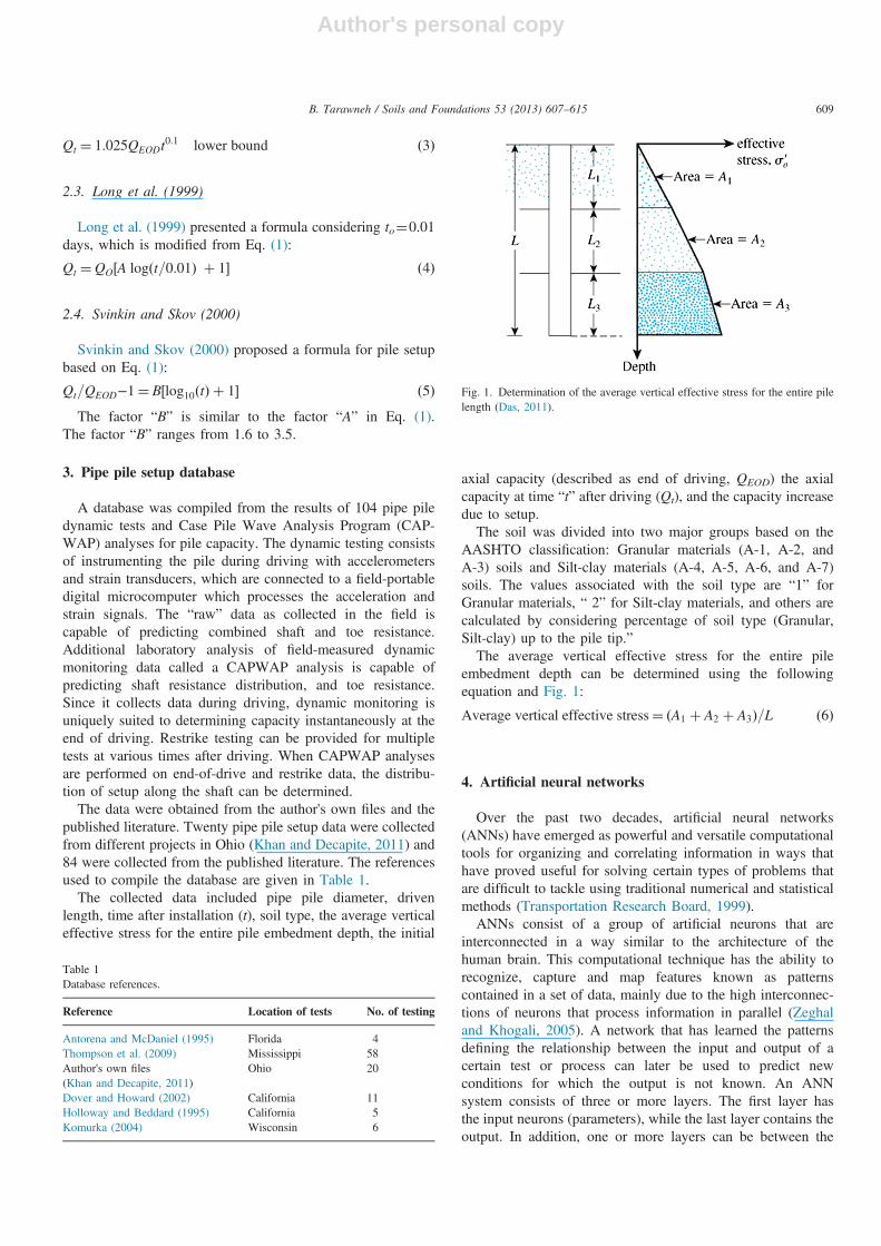
AASHTO classification: Granular materials (A-1, A-2, andA-3) soils and Silt-clay materials (A-4, A-5, A-6, and A-7)soils. The values associated with the soil type are “1” forGranular materials, “ 2” for Silt-clay materials, and others arecalculated by considering percentage of soil type (Granular,Silt-clay) up to the pile tip.”The average vertical effective stress for the entire pile

embedment depth can be determined using the followingequation and Fig. 1:

Average vertical effective stress¼ ðA1 þ A2 þ A3Þ=L ð6Þ

4. Artificial neural networks

Over the past two decades, artificial neural networks(ANNs) have emerged as powerful and versatile computationaltools for organizing and correlating information in ways thathave proved useful for solving certain types of problems thatare difficult to tackle using traditional numerical and statisticalmethods (Transportation Research Board, 1999).ANNs consist of a group of artificial neurons that are

interconnected in a way similar to the architecture of thehuman brain. This computational technique has the ability torecognize, capture and map features known as patternscontained in a set of data, mainly due to the high interconnec-tions of neurons that process information in parallel (Zeghaland Khogali, 2005). A network that has learned the patternsdefining the relationship between the input and output of acertain test or process can later be used to predict newconditions for which the output is not known. An ANNsystem consists of three or more layers. The first layer hasthe input neurons (parameters), while the last layer contains theoutput. In addition, one or more layers can be between the

Table 1Database references.

Reference Location of tests No. of testing

Antorena and McDaniel (1995) Florida 4Thompson et al. (2009) Mississippi 58Author's own files(Khan and Decapite, 2011)

Ohio 20

Dover and Howard (2002) California 11Holloway and Beddard (1995) California 5Komurka (2004) Wisconsin 6

Fig. 1. Determination of the average vertical effective stress for the entire pilelength (Das, 2011).

B. Tarawneh / Soils and Foundations 53 (2013) 607–615 609

Author's personal copy

input and output layers, which are known as the hidden layers.Those layers form the network's means of delineating andlearning the patterns governing the data that the network ispresented with.

There are many ways a neural network can be trained. Theback-propagation technique, which was developed byRumelhart et al. (1986), is the most popular process and hasbeen used in many fields of science and engineering. With thismethod, the weights of the network are adjusted during thetraining phase to minimize error. In each iteration, the errorpropagates backward to minimize the error to a desired level.

In recent years, there has been a growing interest in the useof ANNs in the design of deep and shallow foundations. Orneket al. (2012) presented a study to describe the use of artificialneural networks (ANNs), and the multi-linear regression model(MLR) to predict the bearing capacity of circular shallowfootings supported by layers of compacted granular fill overnatural clay soil. Nejad and Jaksa (2011) developed an ANNmodel to predict pile settlement based on standard penetrationtest data. Abu-Kiefa (1998) introduced three neural networkmodels to predict the capacity of driven piles in cohesionlesssoils. Lee and Lee (1996) utilized neural networks to predictthe ultimate bearing capacity of piles. Chan and Chow (1995)developed a neural network as an alternative to pile drivingformula. Goh (1994a, 1995b) presented a neural networkmodel to predict the friction capacity of piles in clays.

5. Development of ANN model to predict pipe pile setup

The development of an ANN model requires the determina-tion of model inputs and outputs, division and pre-processingof the available data, the determination of appropriate networkarchitecture, stopping, and model validations. Neuro-Solutions6.0 Software was used in creating the neural network models.This software combines a modular design interface withadvanced learning procedures, giving the power and flexibilityneeded to design the neural network that produces the bestsolution.

The data used to develop and validate the neural networkmodel were obtained from both published literature and theauthor's own files. Suitable case studies were those having pileload tests and information regarding the piles and soil. Thedatabase contains a total of 104 cases of pile load tests. Thereferences used to compile the database are given in Table 1.

5.1. Model inputs and outputs

In order to achieve accurate pile setup predictions, athorough understanding of the factors affecting pile setup isneeded. Most of traditional pile setup methods include thefollowing fundamental parameters: pile geometry, pile mate-rial, average effective stress at tip, soil properties, time, andQEOD.

Setup is much affected by soil and pile type. Effective stresschanging with time also has a significant role in the evaluationof pile capacity. The pile length and pile diameter affect setupinfluence zone (Jongkoo, 2007).

In this paper, the factors that are presented to the ANNas model input variables are pile diameter, pile length, soiltype, average effective stress at tip, and the time. Pile capacityincrease due to setup (Qt−QEOD) was the single outputvariable.To identify which of the input variables have the most

significant impact on pile setup prediction, a sensitivityanalysis was carried out on the trained network. A simpleand innovative technique proposed by Garson (1991) was usedto define the relative importance of the input variables byexamining the connection weights of the trained network. Theresults of the sensitivity analysis are discussed later.

5.2. Data division and pre-processing

The data were divided into three sets; training, crossvalidation, and testing. Seventy percent of the data pointswere selected for training, 15% were selected for crossvalidation, and 15% were used for testing the network. Thetraining data points were used to train the network andcompute the weights of the inputs. The test data points wereused to measure the performance of the selected ANN model.The cross validation computes the error of an independent dataset (cross validation data set) at the same time that the networkis being trained with the training set.During training, the input and desired data will be repeatedly

presented to the network. As the network learns, the error willdrop towards zero. Lower error, however, does not alwaysmean a better network. It is possible to over train the network.The network can be over-trained to the point where perfor-mance on new data actually deteriorates. Overtraining resultsin a network that memorizes the individual exemplars ratherthan trends in the data set as a whole. A stopping criteria needsto be established to avoid overtraining. In this paper, crossvalidation was used as the stopping criteria. To stop thetraining of the network; part of the data was set aside for thepurpose of monitoring the training process and to guard againstovertraining. The cross validation set was never used fornetwork weight adjustment.It is important that the data used for training, cross

validation, and testing represent the same population(Masters, 1993) and the statistical properties (e.g. mean,standard deviation and range) of the data subsets need to besimilar (Shahin et al., 2004). Also, ANNs perform best whenthey do not extrapolate beyond the range of their training data(Flood and Kartam, 1994; Tokar and Johnson, 1999). Accord-ingly, in order to develop the best possible model, all patternsthat are contained in the data need to be included in thetraining set. Similarly, since the test set is used to determinewhen to stop training, it needs to be representative of thetraining set and should contain all of the patterns that arepresent in the available data (Shahin et al., 2002). Toaccomplish this, several random combinations of the training,cross validation and testing sets were tried until a statisticallyconsistent data set was obtained. The statistical parametersconsidered include the mean, standard deviation, minimum,maximum and range, as suggested by Shahin et al. (2004).

B. Tarawneh / Soils and Foundations 53 (2013) 607–615610

Author's personal copy

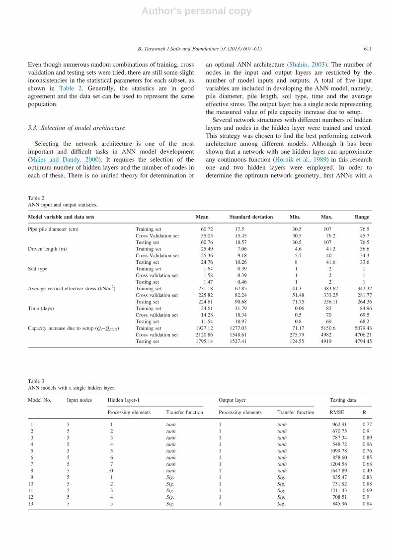
Even though numerous random combinations of training, crossvalidation and testing sets were tried, there are still some slightinconsistencies in the statistical parameters for each subset, asshown in Table 2. Generally, the statistics are in goodagreement and the data set can be used to represent the samepopulation.

5.3. Selection of model architecture

Selecting the network architecture is one of the mostimportant and difficult tasks in ANN model development(Maier and Dandy, 2000). It requires the selection of theoptimum number of hidden layers and the number of nodes ineach of these. There is no unified theory for determination of

an optimal ANN architecture (Shahin, 2003). The number ofnodes in the input and output layers are restricted by thenumber of model inputs and outputs. A total of five inputvariables are included in developing the ANN model, namely,pile diameter, pile length, soil type, time and the averageeffective stress. The output layer has a single node representingthe measured value of pile capacity increase due to setup.Several network structures with different numbers of hidden

layers and nodes in the hidden layer were trained and tested.This strategy was chosen to find the best performing networkarchitecture among different models. Although it has beenshown that a network with one hidden layer can approximateany continuous function (Hornik et al., 1989) in this researchone and two hidden layers were employed. In order todetermine the optimum network geometry, first ANNs with a

Table 2ANN input and output statistics.

Model variable and data sets Mean Standard deviation Min. Max. Range

Pipe pile diameter (cm) Training set 60.72 17.5 30.5 107 76.5Cross Validation set 55.05 15.45 30.5 76.2 45.7Testing set 60.76 18.57 30.5 107 76.5

Driven length (m) Training set 25.49 7.06 4.6 41.2 36.6Cross Validation set 25.36 9.18 5.7 40 34.3Testing set 24.76 10.26 8 41.6 33.6

Soil type Training set 1.64 0.39 1 2 1Cross validation set 1.58 0.39 1 2 1Testing set 1.47 0.46 1 2 1

Average vertical effective stress (kN/m2) Training set 231.18 62.85 41.3 383.62 342.32Cross validation set 225.82 82.24 51.48 333.25 281.77Testing set 224.61 90.68 71.75 336.11 264.36

Time (days) Training set 24.61 31.79 0.06 85 84.96Cross validation set 14.28 18.34 0.5 70 69.5Testing set 11.54 18.97 0.8 69 68.2

Capacity increase due to setup (Qt−QEOD) Training set 1927.12 1277.03 71.17 5150.6 5079.43Cross validation set 2120.86 1548.61 275.79 4982 4706.21Testing set 1795.14 1527.41 124.55 4919 4794.45

Table 3ANN models with a single hidden layer.

Model No. Input nodes Hidden layer-1 Output layer Testing data

Processing elements Transfer function Processing elements Transfer function RMSE R

1 5 1 tanh 1 tanh 962.91 0.772 5 2 tanh 1 tanh 670.75 0.93 5 3 tanh 1 tanh 787.34 0.894 5 4 tanh 1 tanh 548.72 0.965 5 5 tanh 1 tanh 1099.78 0.766 5 6 tanh 1 tanh 858.60 0.857 5 7 tanh 1 tanh 1204.58 0.688 5 10 tanh 1 tanh 1647.89 0.499 5 1 Sig. 1 Sig. 835.47 0.8310 5 2 Sig. 1 Sig. 731.82 0.8811 5 3 Sig. 1 Sig. 1211.43 0.6912 5 4 Sig. 1 Sig. 708.51 0.913 5 5 Sig. 1 Sig. 845.96 0.84

B. Tarawneh / Soils and Foundations 53 (2013) 607–615 611

Author's personal copy

single hidden layer and different number of nodes in thehidden layer are trained with sigmoidal (Sig.) and hyperbolictangent (tanh) transfer functions for the hidden and outputlayers. Combinations of numbers of elements in the hiddenlayer and types of transfer function that yielded the mostaccurate predictions of pile setup are shown in Table 3.

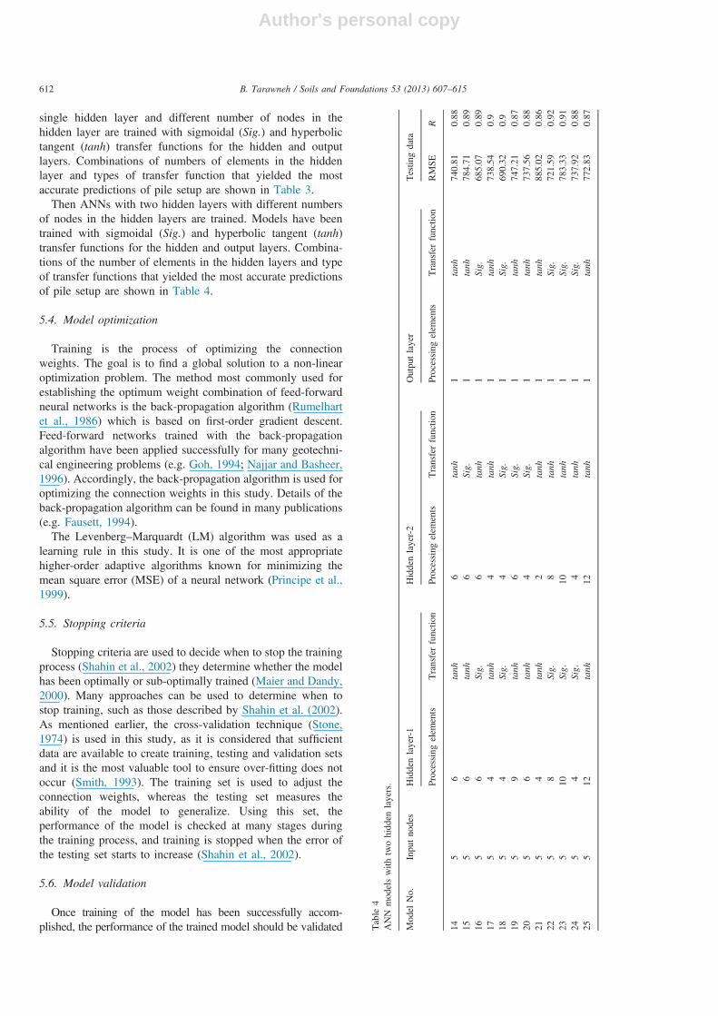
Then ANNs with two hidden layers with different numbersof nodes in the hidden layers are trained. Models have beentrained with sigmoidal (Sig.) and hyperbolic tangent (tanh)transfer functions for the hidden and output layers. Combina-tions of the number of elements in the hidden layers and typeof transfer functions that yielded the most accurate predictionsof pile setup are shown in Table 4.

5.4. Model optimization

Training is the process of optimizing the connectionweights. The goal is to find a global solution to a non-linearoptimization problem. The method most commonly used forestablishing the optimum weight combination of feed-forwardneural networks is the back-propagation algorithm (Rumelhartet al., 1986) which is based on first-order gradient descent.Feed-forward networks trained with the back-propagationalgorithm have been applied successfully for many geotechni-cal engineering problems (e.g. Goh, 1994; Najjar and Basheer,1996). Accordingly, the back-propagation algorithm is used foroptimizing the connection weights in this study. Details of theback-propagation algorithm can be found in many publications(e.g. Fausett, 1994).

The Levenberg–Marquardt (LM) algorithm was used as alearning rule in this study. It is one of the most appropriatehigher-order adaptive algorithms known for minimizing themean square error (MSE) of a neural network (Principe et al.,1999).

5.5. Stopping criteria

Stopping criteria are used to decide when to stop the trainingprocess (Shahin et al., 2002) they determine whether the modelhas been optimally or sub-optimally trained (Maier and Dandy,2000). Many approaches can be used to determine when tostop training, such as those described by Shahin et al. (2002).As mentioned earlier, the cross-validation technique (Stone,1974) is used in this study, as it is considered that sufficientdata are available to create training, testing and validation setsand it is the most valuable tool to ensure over-fitting does notoccur (Smith, 1993). The training set is used to adjust theconnection weights, whereas the testing set measures theability of the model to generalize. Using this set, theperformance of the model is checked at many stages duringthe training process, and training is stopped when the error ofthe testing set starts to increase (Shahin et al., 2002).

5.6. Model validation

Once training of the model has been successfully accom-plished, the performance of the trained model should be validated T

able

4ANN

modelswith

twohidden

layers.

Model

No.

Inputnodes

Hiddenlayer-1

Hiddenlayer-2

Outputlayer

Testin

gdata

Processingelem

ents

Transferfunctio

nProcessingelem

ents

Transferfunctio

nProcessingelem

ents

Transferfunctio

nRMSE

R

145

6tanh

6tanh

1tanh

740.81

0.88

155

6tanh

6Sig.

1tanh

784.71

0.89

165

6Sig.

6tanh

1Sig.

685.07

0.89

175

4tanh

4tanh

1tanh

738.54

0.9

185

4Sig.

4Sig.

1Sig.

690.32

0.9

195

9tanh

6Sig.

1tanh

747.21

0.87

205

6tanh

4Sig.

1tanh

737.56

0.88

215

4tanh

2tanh

1tanh

885.02

0.86

225

8Sig.

8tanh

1Sig.

721.59

0.92

235

10Sig.

10tanh

1Sig.

783.33

0.91

245

4Sig.

4tanh

1Sig.

737.92

0.88

255

12tanh

12tanh

1tanh

772.83

0.87

B. Tarawneh / Soils and Foundations 53 (2013) 607–615612

Author's personal copy

using data sets that have not been used as part of the learningprocess. This data set is known as the testing set. The purpose ofthe model validation phase is to ensure that the model has theability to generalize within the limits set by the training data in arobust fashion, rather than simply having memorized the input–output relationships that are contained in the training data (Shahinet al., 2002).The coefficient of correlation, R; the root meansquared error, RMSE; and the mean absolute error, MAE, are themain criteria that are used to evaluate the prediction performanceof ANN models. The coefficient of correlation is a measure that isused to determine the relative correlation between the predictedand measured data.

The root mean square error, RMSE, is the most popularmeasure of error. It has the advantage that large errors receivemuch greater attention than small errors (Hecht-Nielson,1990). The root mean square error, RMSE, and mean absoluteerror, MAE, are desirable when the data evaluated are smoothor continuous (Twomey and Smith, 1997).

6. Results

For the one hidden layer models, Table 3 shows the resultsof the top performing models. The results showed that the

RMSE values were between 548.72 and 1647.89 and thecoefficient of correlation, R, values were between 0.49 and0.96 for the testing data set. It is noted that model 4, whichused four processing elements in the hidden layer and tanh astransfer function for both hidden and output layer was the bestperforming among all models. It has the lowest RMSE value(548.72) and the highest R value (0.96) for the testing data set.The RMSE for the training and cross-validation data sets were0.22 and 0.57, respectively, for model 4.Table 4 shows the results of the top performing ANN

models with two hidden layers. The results showed that theRMSE values were between 685.07 and 885.02 and thecoefficient of correlation, R, values were between 0.86 and0.92 for the testing data set.It is noted that model 16, which used six processing

elements in each hidden layer, sigmoid as transfer functionfor the first hidden and output layers, and tanh as transferfunction for the second hidden layer, has the lowest RMSE(685.07); R value for this model was 0.89 for the testingdata set.Model 23, which used 10 processing elements in each

hidden layer, sigmoid as transfer function for the first hidden

Table 5Sensitivity analysis of the relative importance (%) for the ANN optimal model.

ANN input variable Relative importance %

Pipe pile diameter 13Driven length 38Soil type 12Average vertical effective stress 23Time 14

0

1000

2000

3000

4000

5000

6000

7000

8000

9000

0 1000 2000 3000 4000 5000 6000 7000 8000 9000

Mea

sure

d Q

t (kN

)

Predicted Qt (kN)

ANNs Optimal Model Skov and Denver Long

Svinkin-Upper Svinkin-Lower Svinkin and Skov

Fig. 2. Measured versus predicted Qt for the optimal ANN model; Skov and Denver (1988), Svinkin (1996), Svinkin and Skov (2000), and Long et al. (1999)formulas.

Table 6Coefficient of determination for measured Qt vs. predicted.

Prediction method Coefficient of determination, R2

ANN-Model-4 0.92Skov and Denver 0.8Long 0.82Svinkin-upper 0.66Svinkin-lower 0.66Svinkin and Skov 0.81

B. Tarawneh / Soils and Foundations 53 (2013) 607–615 613

Author's personal copy

and output layers, and tanh as transfer function for the secondhidden layer, has the highest R value (0.91); the RMSE valuefor this model was 783.33 for the testing data set. The RMSEsfor the training and cross-validation data sets were less than0.25 and 0.6, respectively, for models 16 and 23.

It can be concluded that model 4 is the best performingoptimal model among all ANN models. Based on the availabledata and result, this model can be recommended to predict thepipe pile capacity increase due to setup.

The results of a sensitivity analysis for the optimal model(model 4) with a single hidden layer and four nodes are shownin Table 5. As one would expect, it can be seen that the pilelength, average vertical effective stress, time, pipe pilediameter, and the soil type have the most significant effecton the predicted pipe pile capacity increase due to setup.

7. Numerical model

In this section, the testing data set was used to compare themeasured Qt with the predicted Qt using the optimal ANNmodel (i.e., model 4, with one hidden layer and four nodes inthe hidden layer), as well as Qt predicted using the empiricalformulas presented in Section 2 of this paper. It is known thatthis data set was not included in the training data of the network.Plots of measured versus predicted Qt are shown in Fig. 2 forthe optimal ANN model and the Skov and Denver (1988),Svinkin (1996), Svinkin and Skov (2000), and Long et al.(1999) formulas. It can be seen that the optimal ANN modelsatisfactorily predicted the measured data and significantlyoutperformed the examined empirical formulas.

Table 6 shows the coefficient of determination, R2 for themeasured Qt versus the optimal ANN model and the Skov andDenver, Svinkin, Svinkin and Skov, and Long et al. formulas. Itcan be seen that the optimal ANN model has the highestR2 value.

8. Conclusions

A back-propagation neural network was used to examine thefeasibility of ANNs to predict the pipe pile axial capacityincrease due to setup. A database containing 104 case recordsof field measurements of pipe pile setup was used to developand verify the model. The results indicated that back-propagation neural networks have the ability to predict thesettlement of pile with an acceptable degree of accuracy(R¼0.96, RMSE¼548.72).

The ANN method can be used as a very good tool forestimating pile setup. The ANN Model adequately predictedpile setup and significantly outperformed the examined empiri-cal formulas. The result of this study indicated that ANNsyielded more accurate pile setup predictions than thoseobtained from the traditional methods examined: Skov andDenver (1988), Svinkin (1996), Svinkin and Skov (2000), andLong et al.'s (1999) formulas.

A sensitivity analysis indicated that, as one would expect,pile diameter, pile length, soil type, average effective stress at

tip, and time have the most significant effects on the pipepile setup.

References

Abu-Kiefa, M.A., 1998. General regression neural networks for driven piles incohesionless soils. Journal of Geotechnical and Geoenvironmental Engi-neering – ASCE 124 (12), 1177–1185.

Antorena, J.M., McDaniel T.G., 1995. Dynamic pile testing in soils exhibitingset-up. In: Deep Foundations Institute 20th Annual Members Conferenceand Meeting. Charleston, South Carolina, pp. 17–27.

Axelsson, G. 1998. Long-term increase in shaft capacity of driven piles insand. In: The 4th International Conference on Case Histories in Geotech-nical Engineering, St. Louis, Missouri, pp. 301–308.

Chan, W., Chow, Y.K., 1995. Neural network: an alternative to pile drivingformulas. Journal of Computer and Geotechnics 17 (2), 135–156.

Chow, F.C., Jardine, R.J., Brucy, F., 1998. Effects of time on capacity of pipepiles in dense marine sand. Journal of Geotechnical and GeoenvironmentalEngineering – ASCE 124 (3), 254–264.

Das, B.M., 2011. Principles of Foundation Engineering, Stamford, CT, USA.Dover, A., Howard, R. 2002. High Capacity Pipe Piles at Sanfrancisco

International Airport. Deep Foundations Congress, Geotechnical SpecialPublication, ASCE: 655–667.

Fausett, L., 1994. Fundamentals of Neural Networks: Architecture, Algo-rithms, and Applications. Prentice-Hall, Englewood Cliffs, NJ.

Flood, I., Kartam, N., 1994. Neural networks in civil engineering: principlesand understanding. Journal of Computing in Civil Engineering – ASCE 8(2), 131–148.

Garson, G., 1991. Interpreting neural-network connection weights. AI Expert 6(7), 47–51.

Goh, A., 1994. Seismic liquefaction potential assessed by neural networks.Journal of Geotechnical and Geoenvironmental Engineering-ASCE 120(9), 1467–1480.

Goh, A.T.C., 1994a. Nonlinear modeling in geotechnical engineering usingneural networks. Australian Civil Engineering Transactions 36 (4),293–297.

Goh, A.T.C., 1995b. Empirical design in geotechnics using neural networks.Geotechnique 45 (4), 709–714.

Hecht-Nielson, R., 1990. Neurocomputing. Addison-Wesley, Reading, MA.Holloway, D.M., Beddard, D.L. 1995. Dynamic testing results, indicator pile

test program, I-880, Oakland, California. In: Deep Foundations Institute20th Annual Members Conference and Meeting. Charleston, SouthCarolina, pp. 105–126.

Hornik, K., Stinchcombe, M., White, H., 1989. Multilayer feed forwardnetworks are universal approximators. Neural Network 2, 359–366.

Jongkoo, J. 2007. Fuzzy and Neural Network Models for Analyses of Piles,North Carolina State University.

Khan, L.I., Decapite, K. 2011. Prediction of Pile Set-up for Ohio Soils. ReportNo. FHWA/OH-2011/3, FHWA, U.S. Department of Transportation.

Komurka, V.E., 2004. Incorporating set-up and support cost distributions intodriven pile design. Current Practices and Future Trends in Deep Founda-tions, 125. Geotechnical Special Publications, ASCE/Geo-Institute16–49.

Lee, I.M., Lee, J.H., 1996. Prediction of pile bearing capacity using artificialneural networks. Journal of Computer and Geotechnics 18 (3), 189–200.

Long, J.H., Kerrigan, J.A., Wysockey, M.H. 1999. Measured Time Effects forAxial Capacity of Driven Piling. Transportation Research Record 1663,Paper No.99-1183, pp. 8–15.

Maier, H.R., Dandy, G.C., 2000. Applications of artificial neural net-works toforecasting of surface water quality variables: issues, applications andchallenges. In: Govindaraju, R.S., Rao, A.R. (Eds.), Artificial NeuralNetworks in Hydrology. Kluwer, Dordrecht, The Netherlands, pp.287–309.

Masters, T., 1993. Practical Neural Network Recipes in C++. Academic, SanDiego.

Ng, K., Roling, M., AbdelSalam, S., Suleiman, M., Sritharan, S., 2013a. Pilesetup in cohesive soil. I: experimental investigation. Journal of Geotechni-cal and Geoenvironmental Engineering – ASCE 139 (2), 199–209.

B. Tarawneh / Soils and Foundations 53 (2013) 607–615614

Author's personal copy

Ng, K., Suleiman, M., Sritharan, S., 2013b. Pile setup in cohesive soil. II:analytical quantifications and design recommendations. Journal of Geo-technical and Geoenvironmental Engineering – ASCE 139 (2), 210–222.

Najjar, Y.,Basheer, I. 1996. A neural network approach for site characterizationand uncertainty prediction. ASCE Geotechnical Special Publication, vol.58(1), pp. 134–148.

Nejad, F.P., Jaksa, M.B., 2011. Prediction of pile settlement using artificialneural networks based on standard penetration test data. Journal ofComputer and Geotechnics 36 (7), 1125–1133.

Ornek, M., Laman, M., Demir, A., Yildiz, A., 2012. Prediction of bearingcapacity of circular footings on soft clay stabilized with granular soil. Soilsand Foundations 52 (1), 69–80.

Principe, J., Euliano, N., Lefebvre, W., 1999. Neural and Adaptive Systems:Fundamentals through Simulations. Wiley, New York.

Rumelhart, D.E, Hinton, G.E, Williams, R.J., 1986. Learning internalrepresentation by error propagation. In: Rumelhart, D.E., McClelland, J.L. (Eds.), Parallel Distributed Processing, vol. 1. MIT Press, Cambridge,MA (Chapter 8).

Shahin, M. 2003. Use of Artificial Neural Networks for Predicting Settlementof Shallow Foundations on Cohesionless Soil, University of Adelaide.

Shahin, M.A., Maier, H.R., Jaksa, M.B., 2002. Predicting settlements ofshallow foundations using artificial neural networks. Journal of Geotech-nical and Geoenvironmental Engineering – ASCE 128 (9), 785–793.

Shahin, M.A., Maier, H.R., Jaksa, M.B., 2004. Data division for developingneural networks applied to geotechnical engineering. Journal of Geotechnicaland Geoenvironmental Engineering-ASCE 18 (2), 105–114.

Skov, R. Denver, H. 1988. Time-dependence of bearing capacity of piles. In:The 3rd International Conference on Application of Stress-wave Theory toPiles, Ottawa, Canada, pp. 879–888.

Smith, M., 1993. Neural Networks for Statistical Modeling. Van Nostrand-Reinhold, New York.

Stone, M., 1974. Cross-validatory choice and assessment of statisticalpredictions. Journal of Royal Statistical Society B 36, 111–147.

Svinkin, M.R., 1996. Setup and relaxation in glacial sand-discussion. Journalof Geotechnical and Geoenvironmental Engineering – ASCE 122 (4),319–321.

Svinkin, M.R., Skov, R. 2000. Set-up effect of cohesive soils in pile capacity.In: The 6th International Conference on Application of Stress-wave Theoryto Piles. Sao Paulo, Brazil, pp. 107–111.

Thompson, W.R., Held, L., Say, S., 2009. Test pile program to determine axialcapacity and pile setup for the Biloxi Bay Bridge. Deep FoundationInstitute 3 (1), 13–22.

Transportation Research Board 1999. Use of Artificial Neural Networks inGeomechanical and Pavement Systems, Transportation Research CircularE-C012, Prepared by A2K05(3) Subcommittee on Neural Nets and OtherComputational Intelligence-based Modeling Systems, TransportationResearch Board, Washington, USA.

Tokar, S.A., Johnson, P.A., 1999. Rainfall-runoff modeling using artificialneural networks. Journal of Hydrologic Engineering – ASCE 4 (3),232–239.

Twomey, J. Smith A. 1997. In: N. Kartam, I. Flood, J.H. Garrett (Eds.),Artificial Neural Networks for Civil Engineers: Fundamentals and Applica-tions, ASCE, New York, pp. 44–64.

Yan, W.M., Yuen, K.V., 2010. Prediction of pile set-up in clays and sands.IOP Conference Series: Materials Science and Engineering 10, 1–8.

Zeghal, M., Khogali, W., 2005. Predicting the Resilient Modulus of UnboundGranular Materials by Neural Networks. BCRA, Trondheim, Norway1–9.

B. Tarawneh / Soils and Foundations 53 (2013) 607–615 615