Pine Island Glacier - a 3D full-Stokes model study Dissertation zur Erlangung des Doktorgrades der Naturwissenschaften im Fachbereich Geowissenschaften der Universit¨ at Hamburg vorgelegt von Nina Wilkens aus Berlin Hamburg 2014

Welcome message from author
This document is posted to help you gain knowledge. Please leave a comment to let me know what you think about it! Share it to your friends and learn new things together.
Transcript

Pine Island Glacier -
a 3D full-Stokes model study
Dissertation
zur Erlangung des Doktorgrades
der Naturwissenschaften im Fachbereich
Geowissenschaften
der Universitat Hamburg
vorgelegt von
Nina Wilkens
aus Berlin
Hamburg
2014
Als Dissertation angenommen vom Fachbereich Geowissenschaftender Universitat Hamburg
auf Grund der Gutachten von Prof. Dr. Angelika Humbertund Prof. Dr. Jorn Behrens
Hamburg, den 4. April 2014
Prof. Dr. Christian BetzlerLeiter des Fachbereichs Geowissenschaften
Contents
List of Figures VII
List of Tables XI
Abstract XII
1 Introduction 1
1.1 The Antarctic Ice Sheet . . . . . . . . . . . . . . . . . . . . . . . . . . . . . 21.1.1 Geologic history . . . . . . . . . . . . . . . . . . . . . . . . . . . . . 21.1.2 The marine ice sheet instability . . . . . . . . . . . . . . . . . . . . . 31.1.3 Basal properties . . . . . . . . . . . . . . . . . . . . . . . . . . . . . 5
1.2 Ice sheet models . . . . . . . . . . . . . . . . . . . . . . . . . . . . . . . . . 71.2.1 Approximations . . . . . . . . . . . . . . . . . . . . . . . . . . . . . . 81.2.2 Basal motion . . . . . . . . . . . . . . . . . . . . . . . . . . . . . . . 91.2.3 Grounding line migration . . . . . . . . . . . . . . . . . . . . . . . . 10
1.3 Pine Island Glacier . . . . . . . . . . . . . . . . . . . . . . . . . . . . . . . . 111.3.1 Observations . . . . . . . . . . . . . . . . . . . . . . . . . . . . . . . 121.3.2 Model studies . . . . . . . . . . . . . . . . . . . . . . . . . . . . . . . 13
1.4 Objectives and structure of this study . . . . . . . . . . . . . . . . . . . . . 14
2 Theory 17
2.1 Balance equations . . . . . . . . . . . . . . . . . . . . . . . . . . . . . . . . 172.1.1 Mass balance - Continuity equation . . . . . . . . . . . . . . . . . . 182.1.2 Momentum balance - Momentum equation . . . . . . . . . . . . . . 192.1.3 Energy balance - Heat transfer equation . . . . . . . . . . . . . . . . 20
2.2 Constitutive relation - Rheology of ice . . . . . . . . . . . . . . . . . . . . . 222.2.1 Glen’s flow law . . . . . . . . . . . . . . . . . . . . . . . . . . . . . . 222.2.2 Rate factor . . . . . . . . . . . . . . . . . . . . . . . . . . . . . . . . 242.2.3 Enhancement factor . . . . . . . . . . . . . . . . . . . . . . . . . . . 25
2.3 Overview of equations . . . . . . . . . . . . . . . . . . . . . . . . . . . . . . 262.4 Boundary conditions . . . . . . . . . . . . . . . . . . . . . . . . . . . . . . . 26
2.4.1 Ice surface . . . . . . . . . . . . . . . . . . . . . . . . . . . . . . . . . 272.4.2 Ice base . . . . . . . . . . . . . . . . . . . . . . . . . . . . . . . . . . 282.4.3 Lateral boundaries - Ice divide, calving front and inflow . . . . . . . 30
2.5 Finite element method - FEM . . . . . . . . . . . . . . . . . . . . . . . . . . 322.5.1 Meshing . . . . . . . . . . . . . . . . . . . . . . . . . . . . . . . . . . 322.5.2 Approximation functions - Basis functions . . . . . . . . . . . . . . . 332.5.3 Weighted-integral form . . . . . . . . . . . . . . . . . . . . . . . . . . 342.5.4 Boundary conditions . . . . . . . . . . . . . . . . . . . . . . . . . . . 352.5.5 Assembly . . . . . . . . . . . . . . . . . . . . . . . . . . . . . . . . . 35
III

Contents
2.5.6 Solution . . . . . . . . . . . . . . . . . . . . . . . . . . . . . . . . . . 36
3 The 3D full-Stokes model for Pine Island Glacier 39
3.1 Data . . . . . . . . . . . . . . . . . . . . . . . . . . . . . . . . . . . . . . . . 39
3.1.1 Ice geometry . . . . . . . . . . . . . . . . . . . . . . . . . . . . . . . 40
3.1.2 Grounding line position . . . . . . . . . . . . . . . . . . . . . . . . . 41
3.1.3 Ice rises . . . . . . . . . . . . . . . . . . . . . . . . . . . . . . . . . . 42
3.1.4 Surface temperature . . . . . . . . . . . . . . . . . . . . . . . . . . . 43
3.1.5 Geothermal heat flux . . . . . . . . . . . . . . . . . . . . . . . . . . . 43
3.1.6 Surface velocity . . . . . . . . . . . . . . . . . . . . . . . . . . . . . . 45
3.2 Implementation . . . . . . . . . . . . . . . . . . . . . . . . . . . . . . . . . . 46
3.2.1 Model geometry . . . . . . . . . . . . . . . . . . . . . . . . . . . . . 48
3.2.2 Ice flow model . . . . . . . . . . . . . . . . . . . . . . . . . . . . . . 49
3.2.3 Thermal model . . . . . . . . . . . . . . . . . . . . . . . . . . . . . . 53
3.2.4 Mesh . . . . . . . . . . . . . . . . . . . . . . . . . . . . . . . . . . . . 55
3.2.5 Solver . . . . . . . . . . . . . . . . . . . . . . . . . . . . . . . . . . . 57
3.3 Verification and validation . . . . . . . . . . . . . . . . . . . . . . . . . . . . 58
3.3.1 Ice shelf ramp . . . . . . . . . . . . . . . . . . . . . . . . . . . . . . . 58
3.3.2 MISMIP 3D . . . . . . . . . . . . . . . . . . . . . . . . . . . . . . . . 63
4 Identification of dominant local flow mechanisms 67
4.1 No-slip simulations . . . . . . . . . . . . . . . . . . . . . . . . . . . . . . . . 68
4.1.1 Driving stress . . . . . . . . . . . . . . . . . . . . . . . . . . . . . . . 69
4.1.2 Heat conduction . . . . . . . . . . . . . . . . . . . . . . . . . . . . . 71
4.1.3 Strain heating . . . . . . . . . . . . . . . . . . . . . . . . . . . . . . 72
4.1.4 Internal deformation . . . . . . . . . . . . . . . . . . . . . . . . . . . 76
4.2 Reference simulations . . . . . . . . . . . . . . . . . . . . . . . . . . . . . . 78
4.2.1 Quasi-inversion technique . . . . . . . . . . . . . . . . . . . . . . . . 79
4.2.2 Reference simulation . . . . . . . . . . . . . . . . . . . . . . . . . . . 81
4.2.3 Temperate layer . . . . . . . . . . . . . . . . . . . . . . . . . . . . . 84
4.2.4 Water content . . . . . . . . . . . . . . . . . . . . . . . . . . . . . . 85
4.2.5 Full-Stokes vs. SIA . . . . . . . . . . . . . . . . . . . . . . . . . . . . 86
4.2.6 Sensitivity to geothermal heat flux . . . . . . . . . . . . . . . . . . . 88
4.3 Hydraulic potential . . . . . . . . . . . . . . . . . . . . . . . . . . . . . . . . 90
4.4 Basal roughness . . . . . . . . . . . . . . . . . . . . . . . . . . . . . . . . . . 91
4.5 Discussion . . . . . . . . . . . . . . . . . . . . . . . . . . . . . . . . . . . . . 92
5 Basal sliding 97
5.1 Theory - Basal sliding . . . . . . . . . . . . . . . . . . . . . . . . . . . . . . 97
5.1.1 Hard beds . . . . . . . . . . . . . . . . . . . . . . . . . . . . . . . . . 98
5.1.2 Deformable beds . . . . . . . . . . . . . . . . . . . . . . . . . . . . . 101
5.2 Evaluation method of results . . . . . . . . . . . . . . . . . . . . . . . . . . 102
5.3 Constant sets of sliding parameters p, q and Cb . . . . . . . . . . . . . . . . 104
5.3.1 Simulations . . . . . . . . . . . . . . . . . . . . . . . . . . . . . . . . 104
5.3.2 Discussion . . . . . . . . . . . . . . . . . . . . . . . . . . . . . . . . . 107
5.4 Matching of roughness measure ξ and sliding parameter Cb . . . . . . . . . 110
5.4.1 Simulations . . . . . . . . . . . . . . . . . . . . . . . . . . . . . . . . 112
IV
Contents
5.4.2 Discussion . . . . . . . . . . . . . . . . . . . . . . . . . . . . . . . . . 1165.5 Li-sliding . . . . . . . . . . . . . . . . . . . . . . . . . . . . . . . . . . . . . 117
5.5.1 The two parameter roughness index - ξ2 and η2 . . . . . . . . . . . . 1185.5.2 Assumptions - Controlling obstacle size - Constant CL . . . . . . . . 1195.5.3 Simulations . . . . . . . . . . . . . . . . . . . . . . . . . . . . . . . . 1205.5.4 Discussion . . . . . . . . . . . . . . . . . . . . . . . . . . . . . . . . . 123
5.6 Discussion . . . . . . . . . . . . . . . . . . . . . . . . . . . . . . . . . . . . . 123
6 Conclusions and outlook 127
A 131
A.1 Integration theorems . . . . . . . . . . . . . . . . . . . . . . . . . . . . . . . 131A.1.1 Reynold’s transport theorem . . . . . . . . . . . . . . . . . . . . . . 131A.1.2 Integral formula of Gauss - Divergence theorem . . . . . . . . . . . . 131A.1.3 Integration by parts - Green-Gauss theorem . . . . . . . . . . . . . . 131
Bibliography 133
Acknowledgements 147
V


List of Figures
1.1 Bedrock topography of Antarctica . . . . . . . . . . . . . . . . . . . . . . . 31.2 Schematic of a marine ice sheet on a retrograde bed . . . . . . . . . . . . . 41.3 Bed roughness distribution below the Antarctic Ice Sheet . . . . . . . . . . 61.4 Surface velocity and grounding line positions at Pine Island Glacier . . . . . 13
2.1 Stress-strain relationships . . . . . . . . . . . . . . . . . . . . . . . . . . . . 232.2 Theory - Boundary conditions - Ice surface . . . . . . . . . . . . . . . . . . 272.3 Theory - Boundary conditions - Ice base - floating . . . . . . . . . . . . . . 282.4 Theory - Boundary conditions - Ice base - grounded . . . . . . . . . . . . . 292.5 Theory - Boundary conditions - Ice divide . . . . . . . . . . . . . . . . . . . 302.6 Theory - Boundary conditions - Calving front . . . . . . . . . . . . . . . . . 312.7 Example of a non-uniform FEM mesh on a complex geometry . . . . . . . . 332.8 Linear basis functions . . . . . . . . . . . . . . . . . . . . . . . . . . . . . . 342.9 Quadratic basis functions . . . . . . . . . . . . . . . . . . . . . . . . . . . . 34
3.1 Model region on Antarctica . . . . . . . . . . . . . . . . . . . . . . . . . . . 393.2 Model domain of Pine Island Glacier on a mosaic of satellite images . . . . 403.3 Surface elevation of Pine Island Glacier . . . . . . . . . . . . . . . . . . . . 413.4 Bed topography of Pine Island Glacier . . . . . . . . . . . . . . . . . . . . . 413.5 Different grounding line and ice rise positions at Pine Island Glacier . . . . 423.6 Surface temperature of Pine Island Glacier . . . . . . . . . . . . . . . . . . 433.7 Geothermal heat flux from Shapiro 2004 of Pine Island Glacier . . . . . . . 443.8 Geothermal heat flux from Fox Maule 2005 of Pine Island Glacier . . . . . . 443.9 Geothermal heat flux from Purucker 2012 of Pine Island Glacier . . . . . . 443.10 Location of volcanic center at Pine Island Glacier . . . . . . . . . . . . . . . 443.11 Observed surface velocity field of Pine Island Glacier . . . . . . . . . . . . . 463.12 Screenshot of the COMSOL GUI . . . . . . . . . . . . . . . . . . . . . . . . 473.13 Difference between interpolated data and geometry object at surface . . . . 493.14 Difference between interpolated data and geometry object at base . . . . . 493.15 Model - Boundary conditions - Ice surface . . . . . . . . . . . . . . . . . . . 513.16 Model - Boundary conditions - Ice base . . . . . . . . . . . . . . . . . . . . 513.17 Model - Boundary conditions - Ice divide . . . . . . . . . . . . . . . . . . . 523.18 Model - Boundary conditions - Calving front . . . . . . . . . . . . . . . . . 523.19 Model - Boundary conditions - Inflow . . . . . . . . . . . . . . . . . . . . . 533.20 Function for implementation of the thermal basal boundary condition . . . 553.21 FEM mesh on the 3D Pine Island Glacier model geometry . . . . . . . . . . 563.22 Mesh quality on the 3D Pine Island Glacier model geometry . . . . . . . . . 563.23 Ice shelf ramp - 3D geometry with the flow field . . . . . . . . . . . . . . . . 603.24 Ice shelf ramp - Horizontal velocities . . . . . . . . . . . . . . . . . . . . . . 613.25 Ice shelf ramp - Vertical velocities . . . . . . . . . . . . . . . . . . . . . . . 62
VII
List of Figures
3.26 Ice shelf ramp - Mass balance . . . . . . . . . . . . . . . . . . . . . . . . . . 63
3.27 MISMIP 3D - Perturbed basal friction parameter . . . . . . . . . . . . . . . 64
3.28 MISMIP 3D - Geometry with velocity field . . . . . . . . . . . . . . . . . . 65
3.29 MISMIP 3D - Horizontal surface velocity u at grounding line . . . . . . . . 65
3.30 MISMIP 3D - Horizontal surface velocity v at grounding line . . . . . . . . 65
3.31 MISMIP 3D - Horizontal surface velocity field u . . . . . . . . . . . . . . . . 66
3.32 MISMIP 3D - Horizontal surface velocity field v . . . . . . . . . . . . . . . . 66
3.33 MISMIP 3D - Vertical surface velocity field w . . . . . . . . . . . . . . . . . 66
4.1 Numbering of tributaries on observed surface flow field . . . . . . . . . . . . 67
4.2 SIA basal drag on Pine Island Glacier . . . . . . . . . . . . . . . . . . . . . 70
4.3 Simulated basal drag on Pine Island Glacier . . . . . . . . . . . . . . . . . . 70
4.4 Homologous basal temperature due to heat conduction . . . . . . . . . . . . 71
4.5 Homologous basal temperature - Without strain heating term . . . . . . . . 72
4.6 Homologous basal temperature - With strain heating term . . . . . . . . . . 72
4.7 Source term at base . . . . . . . . . . . . . . . . . . . . . . . . . . . . . . . 73
4.8 Viscosity at base . . . . . . . . . . . . . . . . . . . . . . . . . . . . . . . . . 74
4.9 Effective strain rate at base . . . . . . . . . . . . . . . . . . . . . . . . . . . 74
4.10 First term in source term at base - D1 . . . . . . . . . . . . . . . . . . . . . 75
4.11 Second term in source term at base - D2 . . . . . . . . . . . . . . . . . . . . 75
4.12 Third term in source term at base - D3 . . . . . . . . . . . . . . . . . . . . 75
4.13 Fourth term in source term at base - D4 . . . . . . . . . . . . . . . . . . . . 75
4.14 Fifth term in source term at base - D5 . . . . . . . . . . . . . . . . . . . . . 75
4.15 Sixth term in source term at base - D6 . . . . . . . . . . . . . . . . . . . . . 75
4.16 Surface velocity field - No sliding - Constant temperature . . . . . . . . . . 77
4.17 Difference to observed surface velocity - No sliding - Constant temperature 77
4.18 Surface velocity field - No sliding - Temperature field - Purucker 2012 . . . 77
4.19 Difference to observed - No sliding - Temperature field - Purucker 2012 . . . 77
4.20 Surface velocity field - No sliding - Temperature field - Fox Maule 2005 . . . 77
4.21 Difference to observed - No sliding - Temperature field - Fox Maule 2005 . . 77
4.22 Surface velocity field - No sliding - Temperature field - Shapiro 2004 . . . . 78
4.23 Difference to observed - No sliding - Temperature field - Shapiro 2004 . . . 78
4.24 Spatial distribution of basal sliding parameter β2 . . . . . . . . . . . . . . . 81
4.25 Surface velocity field - Reference simulation - Purucker 2012 . . . . . . . . . 81
4.26 Difference to observed field - Reference simulation - Purucker 2012 . . . . . 81
4.27 Observed surface velocity vs. reference surface velocity . . . . . . . . . . . . 82
4.28 Observed surface velocity vs. angle difference (observed-reference) . . . . . 82
4.29 Homologous basal temperature field - Reference simulation - Purucker 2012 83
4.30 Basal velocity/Surface velocity - Reference simulation - Purucker 2012 . . . 83
4.31 3D homologous temperature field - Reference simulation - Purucker 2012 . . 84
4.32 Temperate layer thickness - Reference simulation - Purucker 2012 . . . . . . 85
4.33 Normed ice thickness vs. homologous temperature and source term . . . . . 85
4.34 Difference with including water content in temperate layer . . . . . . . . . . 86
4.35 Difference with including water content everywhere . . . . . . . . . . . . . . 86
4.36 Location of extracted profiles on reference surface velocity field . . . . . . . 87
4.37 Horizontal and vertical derivatives of extracted profiles . . . . . . . . . . . . 87
4.38 Homologous basal temperature field - Fox Maule 2005 . . . . . . . . . . . . 89
VIII
List of Figures
4.39 Homologous basal temperature field - Shapiro 2004 . . . . . . . . . . . . . . 89
4.40 Homologous basal temperature field - Constant qgeo . . . . . . . . . . . . . 89
4.41 Homologous basal temperature field - Constant qgeo - No friction heating . . 89
4.42 Homologous basal temperature field - Constant qgeo - No friction heating -No source . . . . . . . . . . . . . . . . . . . . . . . . . . . . . . . . . . . . . 89
4.43 Homologous basal temperature field - Artificial qgeo - Volcano . . . . . . . . 89
4.44 Hydraulic potential at Pine Island Glacier . . . . . . . . . . . . . . . . . . . 90
4.45 Hydraulic potential gradient at Pine Island Glacier . . . . . . . . . . . . . . 91
4.46 Single parameter roughness measure ξ at Pine Island Glacier . . . . . . . . 92
4.47 Bed topography at Pine Island Glacier . . . . . . . . . . . . . . . . . . . . . 92
5.1 Weertman’s original obstacle size and spacing . . . . . . . . . . . . . . . . . 98
5.2 Basal velocity due to regelation . . . . . . . . . . . . . . . . . . . . . . . . . 100
5.3 Basal velocity due to enhanced creep . . . . . . . . . . . . . . . . . . . . . . 100
5.4 Surface velocity field - Reference simulation . . . . . . . . . . . . . . . . . . 102
5.5 Homologous basal temperature field - Reference simulation . . . . . . . . . 102
5.6 Partitioning of the surface flow field into subregions for evaluation . . . . . 103
5.7 Surface velocity field - p1q2 . . . . . . . . . . . . . . . . . . . . . . . . . . . 105
5.8 Difference to reference field - p1q2 . . . . . . . . . . . . . . . . . . . . . . . 105
5.9 Surface velocity field - p2q0 . . . . . . . . . . . . . . . . . . . . . . . . . . . 105
5.10 Difference to reference field - p2q0 . . . . . . . . . . . . . . . . . . . . . . . 105
5.11 Surface velocity field - p3q1 . . . . . . . . . . . . . . . . . . . . . . . . . . . 105
5.12 Difference to reference field - p3q1 . . . . . . . . . . . . . . . . . . . . . . . 105
5.13 Surface velocity field - p3q2 . . . . . . . . . . . . . . . . . . . . . . . . . . . 106
5.14 Difference to reference field - p3q2 . . . . . . . . . . . . . . . . . . . . . . . 106
5.15 Surface velocity field - p1q0 . . . . . . . . . . . . . . . . . . . . . . . . . . . 106
5.16 Difference to reference field - p1q0 . . . . . . . . . . . . . . . . . . . . . . . 106
5.17 RMS value vs. sliding law Nr. - Constant parameters . . . . . . . . . . . . 107
5.18 Effective basal pressure at Pine Island Glacier . . . . . . . . . . . . . . . . . 108
5.19 Reduced effective basal pressure at Pine Island Glacier . . . . . . . . . . . . 108
5.20 Simulated basal drag vs. observed surface velocity . . . . . . . . . . . . . . 109
5.21 Simulated basal drag vs. simulated basal velocity . . . . . . . . . . . . . . . 109
5.22 Spatial distribution of basal sliding parameter Cb . . . . . . . . . . . . . . . 110
5.23 Arcuate surface crevasses on satellite image . . . . . . . . . . . . . . . . . . 110
5.24 Normed and inverted single parameter roughness measure ξn . . . . . . . . 111
5.25 Inverted basal sliding parameter Cb for q = 0 . . . . . . . . . . . . . . . . . 111
5.26 Inverted basal sliding parameter Cb for q = 1 . . . . . . . . . . . . . . . . . 111
5.27 Inverted basal sliding parameter Cb for q = 2 . . . . . . . . . . . . . . . . . 111
5.28 RMS value vs. simulation Nr. - Matched parameters . . . . . . . . . . . . . 113
5.29 Surface velocity field - Matched parameters - p1q0 2 . . . . . . . . . . . . . 114
5.30 Homologous basal temperature field - Matched parameters - p1q0 2 . . . . . 114
5.31 Temperate layer thickness - Matched parameters - p1q0 2 . . . . . . . . . . 115
5.32 Temperate layer thickness - Matched parameters - p1q2 11 . . . . . . . . . 115
5.33 Surface velocity field - Matched parameters - p1q1 7 . . . . . . . . . . . . . 115
5.34 Homologous basal temperature field - Matched parameters - p1q1 7 . . . . . 115
5.35 Surface velocity field - Matched parameters - p1q2 11 . . . . . . . . . . . . 116
5.36 Homologous basal temperature field - Matched parameters - p1q2 11 . . . . 116
IX

List of Figures
5.37 Two parameter roughness measure ξ2 at Pine Island Glacier . . . . . . . . . 1185.38 Two parameter roughness measure η2 at Pine Island Glacier . . . . . . . . . 1185.39 RMS value vs. CL . . . . . . . . . . . . . . . . . . . . . . . . . . . . . . . . 1215.40 Surface velocity field and difference to reference - CL = 1Pa−2ma−1 . . . . 1215.41 Surface velocity field and difference to reference - CL = 31.56Pa−2ma−1 . . 1225.42 RMS value vs. results from simulations with constant, matched and Li-
parameters . . . . . . . . . . . . . . . . . . . . . . . . . . . . . . . . . . . . 124
X

List of Tables
3.1 Overview of parameters for the coupled flow model . . . . . . . . . . . . . . 473.2 Overview of variables for the flow model . . . . . . . . . . . . . . . . . . . . 503.3 Overview of variables for the thermal model . . . . . . . . . . . . . . . . . . 543.4 Overview of parameters for the ice shelf ramp . . . . . . . . . . . . . . . . . 593.5 Mesh specifications for the ice shelf ramp . . . . . . . . . . . . . . . . . . . 603.6 Velocity results for the ice shelf ramp . . . . . . . . . . . . . . . . . . . . . . 613.7 Mass balance results for the ice shelf ramp . . . . . . . . . . . . . . . . . . . 63
4.1 Overview of simulations conducted for Section ”No-slip simulations” . . . . 694.2 Overview of simulations conducted for Section ”Reference simulations” . . . 794.3 Overview of results for discussion in Chapter 4 . . . . . . . . . . . . . . . . 93
5.1 Overview of simulations with constant parameter sets . . . . . . . . . . . . 1045.2 Overview of simulations with matched sliding parameters . . . . . . . . . . 112
XI

Abstract
Mass loss from the Antarctic Ice Sheet is found to significantly contribute to eustatic sealevel rise, due to a dynamic response in the system. Pine Island Glacier, a fast flowingoutlet glacier in the West Antarctic Ice Sheet, is located in the Amundsen Sea EmbaymentArea, where the present Antarctic mass loss is concentrated. The observed mass loss inthe area coincides with acceleration and thinning of the glacier, accompanied by a retreatof the grounding line, which is the line of separation between grounded and floating ice.The bed beneath the glacier lies in large parts below sea level, with the bed sloping downaway from the ocean. This setting makes the glacier especially vulnerable to increasingand possibly accelerating retreat.Remote sensing techniques allow only for the surface conditions of glacial systems to benowadays monitored over reasonable temporal and spatial scales. The conditions at thebase, however, are still widely unknown, due to their inaccessibility. This poses a challenge,as basal conditions are a very important component for understanding glacier dynamics.A key technique to bridge this challenge is given by numerical modelling. In glaciologicalstudies flow models are developed, that can either be used to solve in a prognostic mannerover long time scales, being based on approximations to the full system of equations, orto solve diagnostically in high resolution for the full system, to study processes in moredetail.Here we present a model of the later category, a thermo-mechanically coupled 3D full-Stokes ice flow model, which is set up to the region of Pine Island Glacier. It is solvedwith the finite element method, and the prismatic mesh is refined horizontally across thegrounding line, where high resolution is needed. With this coupled flow model we assessthe present thermal and dynamical state of the coupled ice sheet - ice shelf system. Fur-thermore, we develop a method to include measured basal properties into the formulationof the basal sliding law.We find the glacier to be predominantly cold, with most parts of the base being temperate,thus at pressure melting point. The temperate base is a prerequisite for basal sliding,which controls the faster flowing central stream of the glacier. The dominant mechanismsdriving the flow of the different tributaries are diverse. Some are controlled by a strongbed and according high driving stresses. Others are steered by the basal topography andlikely the presence of water saturated marine sediments. Only minor areas are identifiedwith a significantly thick temperate basal layer. Furthermore, we show a connectionbetween the basal roughness and the sliding behaviour of the glacier. A reduced effectivepressure is a key necessity to explain the fast flow towards the grounding line. Thus, athermo-mechanically coupled model, as we presented here, is essential for the inference ofinterrelations between the thermal regime, the basal roughness structure and the flow andsliding conditions.

Zusammenfassung
Der Massenverlust des Antarktischen Eisschildes hat auf Grund einer dynamischen Kom-ponente im System, einen wesentlichen Einfluss auf den Anstieg des eustatischen Meeres-spiegels. Der Pine Island Gletscher, ein schnell fließender Auslassgletscher im Westant-arktischen Eisschild, liegt in einer Region, die an das Amundsen Meer anschließt, und inder sich der aktuelle antarktische Massenverlust konzentriert. Der beobachtete Massenver-lust wird begleitet von einer zunehmenden Beschleunigung des Gletschers, Abnahme derOberflachenhohe und einem Ruckzug der Aufsatzlinie, wo gegrundetes in schwimmendesEis ubergeht. Der Boden unter dem Gletscher liegt zu einem großen Teil unterhalb desMeeresspiegels und neigt sich zum Inland. Diese Situation macht den Gletscher besondersanfallig fur zunehmenden, und eventuell sogar sich beschleunigenden, Ruckzug.Allein die Oberflacheneigenschaften der glazialen Gebiete konnen heute durch Fernerkun-dungsmethoden in relativ hoher raumlicher und zeitlicher Auflosung abgeschatzt werden.Die Bodeneigenschaften unter den eisbedeckten Gebieten hingegen sind weitgehend un-bekannt, weil sie schwer zuganglich sind. Da basale Eigenschaften einen großen Einflussauf die Dynamik des Gletschers haben, stellt dies eine Herausforderung dar. NumerischeModellierung ist eine wichtige Technik, um diese Herausforderungen zu meistern. In glazio-logischen Studien werden meist entweder Modelle entwickelt, die prognostisch uber langeZeitskalen losen konnen, basierend auf einer Nahrungslosung, oder diagnostisch in hoherAuflosung das volle Gleichungssystem losen, um detaillierter Prozesse zu studieren.Hier stellen wir ein Modell der letzteren Sorte vor. Es ist ein thermo-mechanisch gekop-peltes 3D full-Stokes Fließmodell, welches wir auf den Pine Island Gletscher anwenden.Es wird mit der Methode der Finiten Elemente gelost. Das zugrunde liegende prismati-sche Gitter wird horizontal uber der Aufsatzlinie verfeinert, wo besonders hohe Auflosunggefordert ist. Mit diesem gekoppelten Fließmodell berechnen wir den aktuellen thermi-schen und dynamischen Zustand des Gletschersystems, bestehend aus gegrundetem undschwimmendem Eis. Außerdem entwickeln wir eine Methode, mit der gemessene basaleEigenschaften in der Formulierung des basale Gleitens berucksichtigt werden konnen.Wir stellen fest, dass der Pine Island Gletscher vornehmlich von kaltem Eis bestimmt ist,wobei große Teile der Basis temperiert, also am Druckschmelzpunkt, sind. Die temperierteBasis ist eine Voraussetzung fur basales Gleiten, welches das Fließfeld im zentralen Stromdes Gletschers kontrolliert. Die dominierenden Mechanismen, die die einzelnen Zustromeantreiben, sind divers. Einige sind durch einen festen Untergrund und dadurch durchgroße Antriebskrafte bestimmt. Unter anderen wird marines Sediment vermutet, und ih-re Existenz wird durch die basale Topographie und die Fließwege des basalen Wassersbestimmt. Nur in sehr wenigen Regionen wird eine temperierte basale Schicht von nen-nenswerter Dicke vermutet. Außerdem zeigen wir eine Verbindung zwischen der basalenRauigkeit und der Gleitgeschwindigkeit auf. Ein reduzierter effektiver Druck ist eine Er-klarung fur das schnelle Gleiten des Gletschers in der Nahe der Aufsatzlinie. Demnach istein thermo-mechanisch gekoppeltes Fließmodell, wie wir hier prasentieren, gefordert, umdie Wechselwirkungen zwischen dem thermalen Regime, der basalen Rauhigkeitsstrukturund der Fließ- und Gleitbewegungen, zu analysieren.

Chapter 1
Introduction
A topic that will become increasingly important in the future is that of global sea-levelrise and its resulting impact on the coastal zone. A major reservoir of fresh water existspresently in form of the ice sheets on Greenland and Antarctica. The Antarctic Ice Sheetalone holds the potential to raise global sea level by 58m, if fully melted (Fretwell et al.,2013). The contribution to present global sea level rise of 3.1 ± 0.4mma−1 (1993-2006,Nerem et al. (2006)) from the Greenland and Antarctic Ice Sheets is 0.59 ± 0.2mma−1
(1992-2011, Shepherd et al. (2012)). Ice sheets have long been seen to vary substantiallyonly on timescales of centuries to millennia. This view is changing as observations showa much faster response of ice sheets to climatic change. The cause is believed to be adynamic response of ice streams and outlet glaciers in the ice sheet. Hereby not theflow acceleration due to changes in accumulation or surface temperature is dominant,but due to a response to changing basal conditions or changes in the buttressing of iceshelves (Scambos et al., 2004). The ability to make accurate projections for sea levelrise with modelling studies is among other things limited by uncertainties about basalconditions, basal sliding behaviour, ice deformation and interactions with the surroundingocean (IPCC-AR4, 2007).
Ice moves due to a combination of internal deformation and basal sliding. The internaldeformation of ice is nonlinear, increasing approximately proportional to the cube of theapplied stress. For computational efficiency, most simulations over long time scales use asimplified stress distribution. Some of the recent changes observed in ice sheet margins andfast flowing ice streams can not be reproduced by these models. Thus models consideringall stress terms in the momentum balance are needed (IPCC-AR4, 2007), and have re-cently gathered more and more attention, additionally fostered by growing computationalresources.
Strongly affected by changes in flow velocities, grounding line retreat and surface lower-ing in the past decades is the Amundsen Sea Embayment Area (ASEA) in West Antarctica.While the ASEA only holds an area fraction of about 3% of the entire Antarctic Ice Sheet,and about 17.5% of the West Antarctic Ice Sheet (WAIS) (Rignot, 2001; Vaughan et al.,2006; Bindschadler, 2006), it accounted for over 50% of the total mass loss from Antarc-tica between 2002 and 2008 (Horwath and Dietrich, 2009). Associated with this mass lossare two glacier systems located in this area, Thwaites and Pine Island Glacier. WhileThwaites Glacier mainly widened, Pine Island Glacier accelerated, thinned and showedretreat of the grounding line, which separates grounded from floating ice.
In the following we will give an introduction to the Antarctic Ice Sheet (Section 1.1)and its geologic history (Section 1.1.1) to understand the special setting of the WAIS. Asummary of the major aspects of the Marine Ice Sheet Instability hypothesis is given inSection 1.1.2, followed by a section about the basal properties under the WAIS (1.1.3).
1
Chapter 1 Introduction
The instrument to conduct this study is a 3D full-Stokes thermo-mechanically coupledice flow model. To put this into perspective, we give a general introduction to ice sheetmodels (Section 1.2), with a special focus on approximations commonly applied (Section1.2.1) and how basal sliding (Section 1.2.2) and grounding line motion are incorporated(Section 1.2.3).
Finally, the study area of Pine Island Glacier is introduced (Section 1.3), with observa-tions and model studies described in Sections 1.3.1 and 1.3.2, respectively. The objectivesand structure of this study are given in Section 1.4.
1.1 The Antarctic Ice Sheet
The Antarctic continent is almost entirely covered by an ice sheet of varying thickness.This ice sheet is, with an area of ∼ 13.5× 10⁶ km2 and a volume of 25.4× 10⁶ km3, whichincludes the fringing ice shelves, the world’s largest fresh water store (Benn and Evans,2010). The Pacific side of the Transantarctic Mountains roughly divides the AntarcticIce Sheet into two unequal parts, the smaller West Antarctic Ice Sheet (WAIS), with agrounded ice volume of 3 × 10⁶ km3, and the bigger East Antarctic Ice Sheet (EAIS),with a grounded ice volume of 21.7× 10⁶ km3 (Benn and Evans, 2010). The remainder of0.7× 106 km3 of the ice volume is found in the ice shelves surrounding the grounded ice.
1.1.1 Geologic history
West and East Antarctica are geologically distinct. East Antarctica is believed to beprimarily a Precambrian craton older than 500 Ma, while the WAIS is believed to rest ona cluster of four major crustal blocks (Antarctic Peninsula, Thurston Island, Ellsworth-Whitmore mountains and Marie Byrd Land) (Dalziel and Lawver, 2001). These blockshave moved relative to each other and relative to the East Antarctic craton during breakupof Gondwanaland in the Mesozoic, 251 − 65.5Ma ago (Dalziel and Elliot, 1982; Walkerand Geissman, 2009). The force driving these blocks apart was given by a combinationof ridge-crest subduction and a magmatic plume. The crust was stretched and thinnedand crustal gaps where created that filled with mafic intrusions, a magnesium and ironrich rock. The modification continued in the Cenozoic, starting 65.5Ma ago, possiblycaused by plume-driven extensional rifting of the Central West Antarctic basin and ledto continuing volcanic activity and crustal fracturing (Bindschadler, 2006). Jordan et al.(2009) currently find the thinnest crust of the WAIS with ∼ 19 ± 1 km beneath PineIsland Glacier, a potential source of enhanced heat flow and thus modification of the iceflow dynamics above.
The distinct formation history of East and West Antarctica is currently also noticeableat the bed below the ice sheet, shown in Figure 1.1 with the data from Timmermannet al. (2010). The tectonic processes described above created a geologic ’cradle’ under theWAIS (Bindschadler, 2006), such that the bedrock under most of the WAIS lies belowsea level. Also some areas under the EAIS lie below sea level, but would rebound abovesea level, if the ice sheet would be removed (Joughin and Alley, 2011). In total around8.5% of the present day grounded ice sheet volume of Antarctica lies below sea level(Benn and Evans, 2010). There are several indications for the WAIS to have completelyor partially disappeared during past interglacial periods (Scherer et al., 1998; Naish et al.,2009; Pollard and DeConto, 2009). This could be connected to the hypothetical instability
2
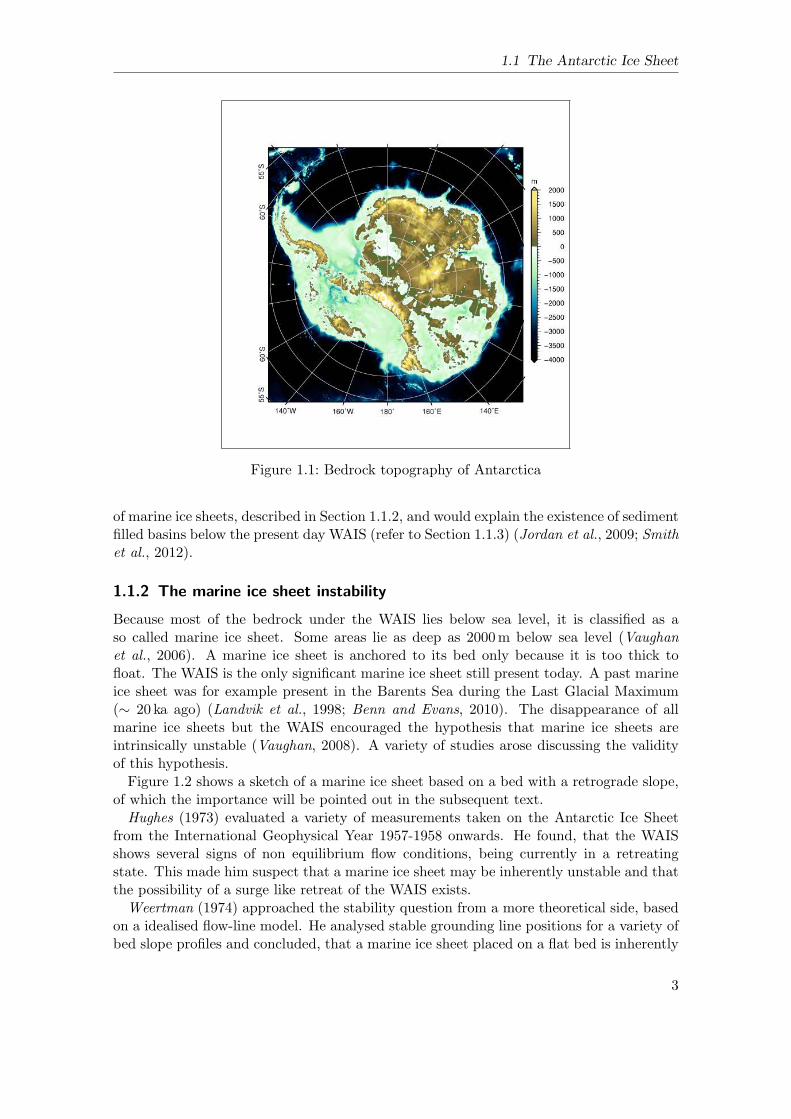
1.1 The Antarctic Ice Sheet
Figure 1.1: Bedrock topography of Antarctica
of marine ice sheets, described in Section 1.1.2, and would explain the existence of sedimentfilled basins below the present day WAIS (refer to Section 1.1.3) (Jordan et al., 2009; Smithet al., 2012).
1.1.2 The marine ice sheet instability
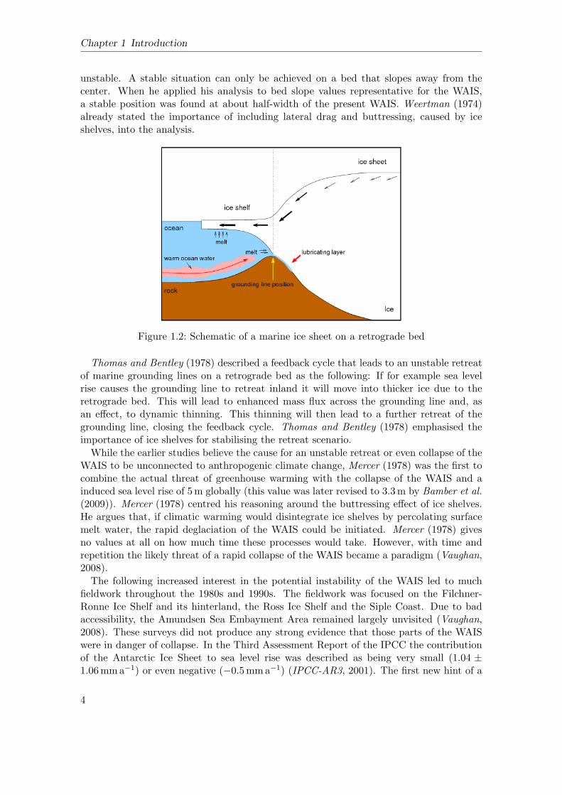
Because most of the bedrock under the WAIS lies below sea level, it is classified as aso called marine ice sheet. Some areas lie as deep as 2000m below sea level (Vaughanet al., 2006). A marine ice sheet is anchored to its bed only because it is too thick tofloat. The WAIS is the only significant marine ice sheet still present today. A past marineice sheet was for example present in the Barents Sea during the Last Glacial Maximum(∼ 20 ka ago) (Landvik et al., 1998; Benn and Evans, 2010). The disappearance of allmarine ice sheets but the WAIS encouraged the hypothesis that marine ice sheets areintrinsically unstable (Vaughan, 2008). A variety of studies arose discussing the validityof this hypothesis.Figure 1.2 shows a sketch of a marine ice sheet based on a bed with a retrograde slope,
of which the importance will be pointed out in the subsequent text.Hughes (1973) evaluated a variety of measurements taken on the Antarctic Ice Sheet
from the International Geophysical Year 1957-1958 onwards. He found, that the WAISshows several signs of non equilibrium flow conditions, being currently in a retreatingstate. This made him suspect that a marine ice sheet may be inherently unstable and thatthe possibility of a surge like retreat of the WAIS exists.Weertman (1974) approached the stability question from a more theoretical side, based
on a idealised flow-line model. He analysed stable grounding line positions for a variety ofbed slope profiles and concluded, that a marine ice sheet placed on a flat bed is inherently
3
Chapter 1 Introduction
unstable. A stable situation can only be achieved on a bed that slopes away from thecenter. When he applied his analysis to bed slope values representative for the WAIS,a stable position was found at about half-width of the present WAIS. Weertman (1974)already stated the importance of including lateral drag and buttressing, caused by iceshelves, into the analysis.
Figure 1.2: Schematic of a marine ice sheet on a retrograde bed
Thomas and Bentley (1978) described a feedback cycle that leads to an unstable retreatof marine grounding lines on a retrograde bed as the following: If for example sea levelrise causes the grounding line to retreat inland it will move into thicker ice due to theretrograde bed. This will lead to enhanced mass flux across the grounding line and, asan effect, to dynamic thinning. This thinning will then lead to a further retreat of thegrounding line, closing the feedback cycle. Thomas and Bentley (1978) emphasised theimportance of ice shelves for stabilising the retreat scenario.
While the earlier studies believe the cause for an unstable retreat or even collapse of theWAIS to be unconnected to anthropogenic climate change, Mercer (1978) was the first tocombine the actual threat of greenhouse warming with the collapse of the WAIS and ainduced sea level rise of 5m globally (this value was later revised to 3.3m by Bamber et al.(2009)). Mercer (1978) centred his reasoning around the buttressing effect of ice shelves.He argues that, if climatic warming would disintegrate ice shelves by percolating surfacemelt water, the rapid deglaciation of the WAIS could be initiated. Mercer (1978) givesno values at all on how much time these processes would take. However, with time andrepetition the likely threat of a rapid collapse of the WAIS became a paradigm (Vaughan,2008).
The following increased interest in the potential instability of the WAIS led to muchfieldwork throughout the 1980s and 1990s. The fieldwork was focused on the Filchner-Ronne Ice Shelf and its hinterland, the Ross Ice Shelf and the Siple Coast. Due to badaccessibility, the Amundsen Sea Embayment Area remained largely unvisited (Vaughan,2008). These surveys did not produce any strong evidence that those parts of the WAISwere in danger of collapse. In the Third Assessment Report of the IPCC the contributionof the Antarctic Ice Sheet to sea level rise was described as being very small (1.04 ±1.06mma−1) or even negative (−0.5mma−1) (IPCC-AR3, 2001). The first new hint of a
4
1.1 The Antarctic Ice Sheet
transient behaviour was given by a study from Wingham et al. (1998), in which elevationchange over about 50% of the continental area was calculated. This was only possible dueto satellite altimeter measurements. Wingham et al. (1998) found, in the period from 1992to 1996, no significant elevation change over most parts of the EAIS. But in the ASEAthey found an indication of surface lowering of as much as 10 cma−1. Due to very highrates of snowfall in this area, Wingham et al. (1998) were not sure if the surface loweringwas due to a dynamic change. But in combination with another study by Rignot (1998),that showed a grounding line retreat at Pine Island Glacier of almost 1 kma−1 over theperiod 1992-1996, the signal for an ongoing dynamic change became clearer.
The observations in the ASEA, and especially at Pine Island Glacier, continued andrevealed a variety of further indications for change. These findings will be further discussedin Section 1.3. Following the observations of change in the ASEA, an additional focus wasset on modelling the transition zone between the grounded and floating ice, the groundingline, described in Section 1.2.3.
1.1.3 Basal properties
For the dynamics of an ice sheet, the basal properties below the ice sheet are important.The ice can exhibit very different basal motion over for example hard rock, till or marinesediments. The availability of liquid water also has a major influence on the basal motionof the ice sheet. In Antarctica the bed rock is a mosaic of hard rock and soft sediments,above which the fast ice streams flow (Benn and Evans, 2010).
It poses a big challenge to derive information on different basal conditions under icesheets. Bore holes are one possibility to obtain information on basal properties. However,only very few boreholes in the WAIS exist (e.g. Engelhardt et al., 1990; Engelhardt andKamb, 1998), as their retrieval is time consuming and expensive. Additionally, they giveonly a random sample at one point in time. This might be important to consider in areaswith fast changing basal conditions, but is not of major concern in slow changing areas.
To derive a spatially more complete picture of the basal properties geophysical tech-niques and modelling are applied (Bingham et al., 2010). The geophysical techniquesinclude RAdio Detection And Ranging (RADAR), seismic and gravity techniques. Theradar systems applied today are mainly airborne and facilitate comprehensive coverage.Cold ice is transparent to electromagnetic waves in the high to very high frequency bands.Thus the Ice-Penetrating Radar (IPR, also called Radio-Echo Sounding (RES)) can detectthe ice surface, internal layers and the ice-bed interface.
The bed-echo strength, also called bed reflectivity, is influenced by the presence of water,subglacial geology and roughness of the ice-bed interface. Brighter reflections can indicatewet, hard and smooth beds, while dimmer reflections indicate dry/frozen, soft/unconsoli-dated and rough beds (Peters et al., 2005). Thus also the possible existence of subglaciallakes can be inferred from bed reflectivity.
Apart from the bed reflectivity, which focuses on the amplitude of the returned signal,it is possible that also the length and phase of the returned signal can be related to basalproperties (Rippin et al., 2006; Bingham et al., 2010).
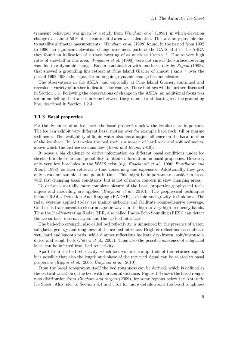
From the basal topography itself the bed roughness can be derived, which is defined asthe vertical variation of the bed with horizontal distance. Figure 1.3 shows the basal rough-ness distribution from Bingham and Siegert (2009), for some regions below the AntarcticIce Sheet. Also refer to Sections 4.4 and 5.5.1 for more details about the basal roughness
5
Chapter 1 Introduction
measure. There are a variety of algorithms for assessing bed roughness, but they all leadto similar regional-scale patterns (Bingham et al., 2010). Here it has to be kept in mind,that high resolution data is only obtained along flight tracks and interpolation betweentracks is applied. This is especially important to consider in data-sparse regions.
Figure 1.3: Bed roughness distribution below the Antarctic Ice Sheet. Figure taken fromBingham and Siegert (2009).
Seismic techniques are the oldest geophysical methods in glaciology and provided thefirst ice thickness measurements of the WAIS (Mothes, 1926; Bentley and Ostenso, 1961).Seismic techniques work with elastic waves, in contrast to electromagnetic waves, and canhence image sub-bed structures. It is thus possible to extract the porosity, compositionand internal structure of subglacial sediments, which can play an important role for fastice flow due to internal sediment deformation (Boulton and Hindmarsh, 1987; van derMeer et al., 2003). Also the existence of a subglacial water layer is possible to detect withseismic methods (King et al., 2004; Smith, 2007).
Inverse modelling techniques are applied with increasing frequency to infer basal prop-erties, such as certain sliding parameters in sliding laws and basal drag (MacAyeal, 1992;Sergienko et al., 2008; Joughin et al., 2009; Pollard and DeConto, 2012). These techniquesare usually based on measured surface velocity fields and use control methods to infer thebasal fields. Modelling of ice flow dynamics is also an important tool to test hypothesesabout subglacial bed properties (Bingham et al., 2010).
From aerogravity measurements the crustal thickness can be inferred and thus a geother-mal heat flux estimated (Jordan et al., 2009). Geothermal heat flux is not directly con-sidered a basal property, but can lead to enhanced subglacial melt water occurrence.
When modelling ice sheet dynamics, not only the type of bed rock can have a majorinfluence, but also the resolution on which the data is available (Durand et al., 2011).
6
1.2 Ice sheet models
1.2 Ice sheet models
For the formation of ice sheet models a variety of developments in different fields werenecessary. There is the development of a physical description of glacier flow, and measure-ments that support the theories. Furthermore, the growing availability of computationalresources fostered the field of numerical modelling. Here we will give a short overview ofthe different developments, followed by descriptions of some selected sub-items in glaciermodelling. First we will have a look at different approximations used in glacier models(Section 1.2.1), followed by basal sliding (Section 1.2.2) and finally grounding line migra-tion in numerical models (Section 1.2.3).Observations of glacier flow, and attempts for a physical explanation, can already be
found in the 18th century. David Forbes (1809-68) was perhaps the first to propose thatglaciers flow like viscous fluids (Clarke, 1987; Blatter et al., 2010). Forbes’ suggestion ledto a heated controversy, due to the solid and brittle appearance of the ice (Cuffey andPaterson, 2010), but eventually prevailed. Laboratory experiments suggested a power-lawfor the deformation of ice (Glen, 1952; Steinemann, 1954; Glen, 1955), in more detail de-scribed in Section 2.2. Nye (1953) applied this power-law for the flow of ice, later calledGlen’s flow law or Glen-Steinemann flow relation, to field observations. It was eventu-ally agreed on, that glacier flow is a problem within the field of fluid dynamics (Blatteret al., 2010). The fluid dynamical balance equations, together with a non-Newtonian rhe-ology, can therefore describe the flow of glacier ice. Due to special properties of glacierice, discussed in Section 2.1.2, the momentum balance becomes a force balance, given incomponents, such that
div(τ − pI) = −ρig ⇒
∂∂xτxx + ∂
∂yτxy + ∂∂zτxz = ∂
∂xp∂∂xτyx + ∂
∂yτyy + ∂∂zτyz = ∂
∂yp∂∂xτzx + ∂
∂yτzy + ∂∂zτzz = ∂
∂zp + ρig,
(1.1)
with τ ij being the different components of the deviatoric stress tensor τ , p the pressure, Ithe identity matrix, ρi the ice density and g the gravitational acceleration. For a derivationof the equations refer to Section 2.1.2. The colour indication will be used in Section 1.2.1to describe the different approximations.In a variety of scientific fields, numerical modelling has become a useful tool to expand
understanding. Especially when real experiments and analytical theory reach their limits.This is among others the case for fluid dynamics. The equations of motion describingfluid flow are well known. But due to nonlinearities in many cases they can not be solvedanalytically. In Computational Fluid Dynamics the equations are solved numerically andthis helps to understand the dynamics of fluid motion.In the past decades the use of computer models in science has become increasingly pop-
ular. The experiments conducted with computer models are called in-silico experiments.This term is an analogue to in-situ, which is a Latin phrase meaning in position. In-silicorefers to the material silicium, what most Central Processing Units (CPUs) are made of(Gramelsberger, 2010).
A glacier model is always a simplification of the reality, with several approximations andassumptions made. Continuum mechanics approximate the fluid motion by the Euleriandescription, which assumes a continuous mass rather than discrete particles. To receivea numerical solution, the underlying system of equations needs to be dicretized (refer toSection 2.5). The grid spacing hereby depends on the focus of the study. In general it
7
Chapter 1 Introduction
can be said that processes that take place on scales smaller than the grid spacing haveto be parametrised, which is the aim to find a formulation for the larger scale impact ofsmaller scale processes. An example for this in glacier models is the sliding of a glacier overits bed. In reality it is influenced by numerous processes on a variety of scales. Slidingrelations are introduced, that try to capture the main processes without becoming toocomplex to work with. Another example is given by the ice rheology, discussed in detailin Section 2.2.1. It describes the bulk creep behaviour of polycrystalline ice, instead of thedeformation of every single ice crystal (van der Veen, 2002; Benn and Evans, 2010).
Another source of uncertainty can be given by the data used to calibrate the model.Measured data is also subject to assumptions and approximations made during the mea-surement process, and has to be handled with care.
Apart from these obvious shortcomings, computer experiments are a valuable tool toinvestigate systems that are not otherwise manageable for a real physical experiment, dueto huge spatial or temporal scales, as is the case for glaciers. Still, when dealing withcomputer experiments, it is very important to remember the shortcomings of the tool. Acommon mistake is for example done by using the same data to validate a model, thatwas initially used to calibrate the system with (van der Veen, 1999).
1.2.1 Approximations
A glacier flow model consists of solving a coupled thermomechanical problem. This canbe done for either a diagnostic or a prognostic problem. Diagnostic models usually focuson particular processes and their influence on the glacier system, while prognostic modelsusually simulate the evolution of glacier systems in time and their response to changingexternal conditions (Benn and Evans, 2010).
When solving the coupled thermomechanical problem, the computationally most ex-pensive part is given by the mechanical part as shown in component form in Eq. (1.1).Solving for the full set of terms is the most exact solution that can be obtained and themodels doing this are called full-Stokes (FS) models (Alley et al., 2012). As these modelsare computational expensive they are usually used diagnostically to study specific outletglaciers (e.g. Morlighem et al., 2010). Increase in computational resources make it alsopossible to calculate the evolution of an ice sheet with a full-Stokes model over a certainperiod (e.g. Seddik et al., 2012).
Depending on the flow regime modelled, different terms in Eq. (1.1) can be shownto have minor influence and can therefore be neglected. The first three dimensional icesheet models were based on the so called Shallow Ice Approximation (SIA) (Hutter, 1983;Morland, 1984). These models assume, that ice flow is dominated by internal shear defor-mation. This is true for large parts of the interior of an ice sheet, where the ice is frozento the ground or the ice simply does not slide due to the high basal roughness. Also inthe interior of an ice sheet typical horizontal extents are large compared to typical verticalextents. Therefore, longitudinal derivatives of stress, velocity and temperature are smallcompared to vertical derivatives and can be neglected (Hooke, 2005). This leaves only theblack and red terms in Eq. (1.1), leading to a local balance of the stresses.
In ice shelves or fast flowing outlet glaciers vertical shear is negligible and horizontalvelocity components therefore hardly vary with depth. The resulting flow is a so calledplug-flow and described by the blue and black terms in Eq. (1.1). This approximationwas first introduced by Morland (1987) for an unconfined ice shelf, and later on extended
8
1.2 Ice sheet models
by MacAyeal (1989) for ice stream flow over a viscous basal sediment. The approximationis called Shelfy-Stream or Shallow Shelf Approximation (SSA).A Higher Order Model (HOM) was first introduced by Blatter (1995) and later on
written in terms of velocities by Pattyn (2003). It incorporates longitudinal stress termsand only neglects part of the brown and red terms in Eq. (1.1).Approximations always simplify the solution and if the requirements for its validity in
certain applications are not considered, this can lead to errors. The SIA is for examplenot valid in key areas such as ice divides and grounding lines (Baral et al., 2001; Pattynet al., 2012). In general the accuracy of the SIA decreases, as the contribution of basalslip increases (Gudmundsson, 2003).
1.2.2 Basal motion
The overall glacier motion consists of different components: internal creep deformationof the ice, sliding of ice over its bed and deformation of the bed itself. Basal motion orbasal slip is the combined motion of sliding and bed deformation (Cuffey and Paterson,2010). The strength, with which the components contribute to the total motion, stronglyvaries in different regions. In certain areas basal sliding can account for up to 90%of the glacier motion (Schweizer, 1989). It is agreed on, that basal slip can be a veryimportant factor for ice dynamics, but still it is difficult to be precisely described in iceflow models, as it depends on many different and often locally unknown factors. A majordrawback to the understanding of basal slip is the difficulty to observe it. Measurementshave been conducted in subglacial cavities, tunnels and boreholes, but these are localmeasurements and can not necessarily be generalised to a wider area (Cuffey and Paterson,2010). Although it might be impossible to know the basal conditions below a glacier wellenough to accurately predict the rate of motion of the glacier over its bed, it is importantto understand the processes, to place limits on the rate (Hooke, 2005). Theories wereestablished to describe the slip mechanisms, with reasonable assumptions made wherenecessary, as a substitute for detailed data. For modelling glacier dynamics slip relationsare necessary. These relations commonly connect basal velocity ub, basal shear stress τ b
and bed characteristics. The bed characteristics can be the effective pressure Nb, the bedroughness and sediment properties (Cuffey and Paterson, 2010). When choosing a slidingrelation for a glacier model, it is often a trade off between a realistic description and aworkable formulation (Benn and Evans, 2010).Following Weertman (1957), the sliding of a glacier over a hard bed is only possible for
a temperate base, which is a base at pressure melting point, and due to a combinationof regelation and enhanced creep. Regelation describes a process where the ice melts dueto high pressure on one side of an obstacle and refreezes on the other side. Enhancedcreep is due to a stress concentration on the upstream side of an obstacle. It was laterfound that sliding velocities exceeding 20ma−1 on hard beds can only be explained withthe existence of water filled cavities, stressing the importance of the effective pressure Nb
(Lliboutry, 1968; Bindschadler, 1983). While the original sliding law by Weertman (1957),described in detail in Section 5.1.1, consisted mainly of physical parameters, it developedinto a general sliding relation of a similar form, the so called Weertman type sliding law
ub ∼ τpb N
−qb . (1.2)
The constants p and q are usually empirically determined. The effective pressure Nb has
9

Chapter 1 Introduction
to be either explicitly modelled as a subglacial hydraulic system (e.g. Flowers et al., 2003)or a simple parametrisation is used (e.g. Huybrechts and de Wolde, 1999). The Weertmantype sliding law in Eq. (1.2) is often extended with a temperature function f(T ), tocontrol sliding for regions with temperatures below pressure melting point (e.g. Fowler,1986; Budd and Jenssen, 1987).
One shortcoming of the above formulation is, that it results in infinite basal velocitiesub → ∞, if Nb = 0 and τ b > 0. This would not happen in reality, as part of thedriving stress is supported by lateral drag and longitudinal stress gradients, so calledglobal controls (Benn and Evans, 2010). Looking at this from another side, for increasingbasal velocities ub ↑ and increasing effective pressure Nb ↑, there is no upper bound forthe basal shear stress τ b, such that τ b < τ b,max. In reality though, cavities form as aresult of increasing water pressure in the lee side of bedrock obstacles, putting an upperbound on τ b, determined by the slope of the bed (Iken, 1981; Schoof, 2005). Relations ofthe form shown in Eq. (1.2), that express the basal velocity ub explicitly as a function ofbasal shear stress τ b and effective pressure Nb, are called sliding laws and implementedas a Dirichlet boundary condition. Laws with an upper bound for τ b, that describe arelationship between the different terms, are called friction laws and implemented as aRobin boundary condition (Gagliardini et al., 2007). These friction laws can be multi-valued, meaning a given basal velocity may be associated with more than one value ofbasal drag (Benn and Evans, 2010).
The above described sliding and friction laws only deal with hard bed sliding. Ondeformable substrates, hereafter generally referred to as till, high basal velocities can alsobe present (Cuffey and Paterson, 2010). Subglacial till can consist of glacial depositsor marine sediments. It can be modelled separately to derive the internal temperaturedependent deformation (e.g. Bougamont et al., 2003; Christoffersen and Tulaczyk, 2003).These models are based on a Coulomb-plastic yield criterion, which specifies the maximumbasal shear stress τ b that can be supported by the till (Benn and Evans, 2010).
In reality many regions are dominated by a mixture of hard (bedrock) and soft or weak(till) beds. Simple parametrisations can be used to capture this by applying a law of the
form τ b ∼ u1/mb , where m = 1 should mimic linear-viscous till deformation (MacAyeal,
1992), m→ ∞ plastic till behaviour or fast flow over hard bed (Joughin et al., 2004) andm = 3 slow flow over hard bed (Cuffey and Paterson, 2010).
1.2.3 Grounding line migration
The dynamics of marine ice sheets are sensitive to grounding line position and migration.Thus grounding line motion is an important factor for numerical investigation of the WAIS(Katz and Worster, 2010). Many current ice-sheet models do not yet include rapid ice lossdue to grounding line migration, as most of the complex processes are poorly understood(Docquier et al., 2011).
The different stress approximations in ice sheet models (Section 1.2.1) lead to differentimplementations of grounding line motion. For grounding line motion it is also of highimportance what kind of mesh is applied. In Fixed Grid (FG) models the groundingline position always falls in between grid points. Moving Grid (MG) models explicitlymodel the position and follow it continuously. Adaptive Mesh (AM) models are a trade-off between fixed and moving grids, and refine the mesh near the grounding line (Docquieret al., 2011).
10

1.3 Pine Island Glacier
Some full-stokes models solve a contact problem between the ice and a rigid bedrock(Durand et al., 2009). To determine the location of the grounding line two conditions haveto apply, the floating condition and a stress condition, comparing the water pressure tothe ice overburden pressure (Schoof, 2005; Gagliardini et al., 2007; Durand et al., 2009).Another way is to determine the grounding line position by solving for the ice thicknessand apply the floating condition, hereby neglecting bridging effects (Pattyn et al., 2013).
Several studies show, that it is necessary to consider all stress terms in the transitionzone from shear flow to plug flow across the grounding line (e.g. Lestringant, 1994; Pattyn,2000; Pattyn and Durand, 2013). For large scale ice sheet models, this is not possible,due to computational costs. Schoof (2007a) developed a semi-analytical solution for theice flux across the grounding line for shallow models, which Pollard and DeConto (2009)incorporated into a numerical ice sheet model at coarse grid resolution by applying aheuristic rule.
Mesh resolution around the grounding line is also a crucial issue (Vieli and Payne, 2005).High mesh resolution is needed in the vicinity of the grounding line in order to generateconsistent results (Durand et al., 2009; Gladstone et al., 2012). To save computationalcost, ice sheet models with adaptive mesh refinements are of high interest and increasinglydeveloped (e.g. Gladstone et al., 2010; Cornford et al., 2012).
For the hypothesis of marine ice sheet instability, the existence of steady state groundingline positions on reverse bed slopes is discussed. There are studies that suggest neutralequilibrium on a reversed bed slope (e.g. Hindmarsh, 1993, 1996) and others, that do not(e.g. Schoof, 2007a; Durand et al., 2009; Katz and Worster, 2010). The Marine Ice SheetModel Intercomparison Project (MISMIP) shows common agreement on the hysteresisacross an overdeepend bed for 2D flow-line models (Pattyn et al., 2012). Newer 3D modelstudies, however, stress the importance of lateral drag and are able to produce steadygrounding line positions on a reversed bed slope (Gudmundsson et al., 2012; Jamiesonet al., 2012).
A new Marine Ice Sheet Model Intercomparison Project for 3D models (MISMIP 3D)was conducted, which focuses on the reversibility of grounding line positions and noton reversed bed slopes though (Pattyn et al., 2013). These model intercomparisons arevaluable to estimate the influence of model physics, approximations, grid resolutions andother factors onto the results of grounding line positions.
1.3 Pine Island Glacier
Pine Island Glacier is a fast flowing outlet glacier, draining a large part of the WAIS. Inthe past decades the glacier has shown acceleration, thinning and a significant groundingline retreat (Rignot, 2008; Wingham et al., 2009; Rignot, 1998). These ongoing processesare coinciding with a concentrated mass loss in the area around Pine Island Glacier, theAmundsen Sea Embayment (Horwath and Dietrich, 2009).
While the Weddell and Ross Sea sectors drain through ∼ 500 km wide ice shelves, theAmundsen Sea sector holds only narrow ice shelves, that provide less buffering againstcollapse. Due to this special setting, Mercer (1978) identified the Amundsen Sea sector asthe most vulnerable to collapse.
In the following we will give an overview of the observed changes on Pine Island Glacier(Section 1.3.1) and the conducted model studies for this area (Section 1.3.2).
11

Chapter 1 Introduction
1.3.1 Observations
Observations on Pine Island Glacier became denser in the 1970s with increasing satelliteobservations. Earlier observations were sparse due to the remoteness of the glacier and anextensive sea ice cover in Pine Island Bay (Vaughan, 2008).
Pine Island Glacier drains an area of ∼ 1.75× 10⁶ km2 (Vaughan et al., 2006), which isabout 9% of the WAIS. From the total potential of the WAIS to raise eustatic sea levelby 3.3m (Bamber et al., 2009), 0.52m can be accounted to Pine Island Glacier (Vaughanet al., 2006). In case of a collapse of the WAIS, only 0.24m from those 0.52m of iceequivalent would really be lost to the ocean, as the drainage basin is subdivided into anorthern and southern basin by a bed high (Vaughan et al., 2006).
Under Pine Island Glacier sediment basins are suspected. Their existence is inferredfrom basal roughness distributions (Rippin et al., 2011), aerogravity measurements (Jordanet al., 2009) and seismics (Smith et al., 2013). Subglacial geology influences the spatialpattern of ice flow (Smith et al., 2013). In some areas, subglacial erosion rates of ∼ 1ma−1
have been derived (Smith et al., 2012), suggesting a possible change over time of thesubglacial environment, and thus possibly the ice flow patterns.
The fast flowing (|us| > 100ma−1) main trunk of the glacier is about 325 km long,while the total length from the ice divide to the calving front is about 400 km. The maintrunk lies in a 500m deep trough, which suggests a constrained and long-lived ice stream(Vaughan et al., 2006).
The ice flows from the interior to the West, into the Amundsen Sea, where it formsa small ice shelf. The shape of the ice shelf is defined by a variety of ice rises, pinningthe ice shelf. The areal extent of the ice shelf has not shown major changes since ob-servations started in 1947, only the slow flowing northern shelf showed a slight ongoingretreat. The calving front undulates with calving events periodically about every 6 years(1995/96,2001,2007,2013) (Rignot, 2002, pers. observation). At these calving events, bigicebergs, several km long and 10−20 km wide, are calved off into the Amundsen Sea. Theiceberg size for the last big calving event in 2013 was ∼ 700 km2 (pers. observation).
Beneath the ice shelf a ridge is located in the sea bed, perpendicular to the flow direction.The position of the ridge is suggested to be an earlier location of the grounding line(Jenkins et al., 2010). In the past decades, the grounding line position strongly retreatedfurther by 1.2± 0.3 km between 1992 and 1996 (Rignot, 1998), and up to 20 km between1996 and 2009 (Joughin et al., 2010). For a further description also refer to Section3.1.2. This recent retreat took place across a so called ice plain, an only slightly groundedarea, which facilitated the ungrounding (Corr et al., 2001). The grounding line positionin 2009 includes a lightly-grounded island like area forward of the main grounding line(Joughin et al., 2010). Park et al. (2013) infer from 1992 to 2011 a constant retreat rateof 0.95±0.09 kma−1, which is accompanied by an accelerated rate of terminus thinning of0.53± 0.15ma−2. Figure 1.4, taken from Joughin et al. (2010), shows the surface velocityfield at Pine Island Glacier, together with the grounding line positions from 1996 and2009.
Acceleration of the entire glacier flow speed has been observed since the 1970s. The iceshelf, which is only the part of the glacier floating on the ocean, accelerated hereby from∼ 2300ma−1 in 1974 to ∼ 4000ma−1 in 2007. The entire glacier, including grounded andfloating ice, accelerated by 42% between 1996 and 2007 and by 73% between 1974 and2007 (Rignot, 2008).
12

1.3 Pine Island Glacier
Figure 1.4: Surface velocity and grounding line positions 1996 (cyan) and 2009 (magenta).Figure taken from Joughin et al. (2010).
This acceleration is accompanied by an increased thinning near the grounding line from3ma−1 in 1995 to 10ma−1 in 2006. In 1995, the thinning was limited to the main trunkof the glacier, with thinning rates over 1ma−1 confined to the ice plain area. By 2006 thethinning was found in all the tributaries with rates over 1ma−1 extending up to 100 kminland from the grounding line (Wingham et al., 2009).
Warm ocean waters are suspected to be a major driver for these ongoing observedchanges (Payne et al., 2004; Jacobs et al., 2011; Pritchard et al., 2012). Different ap-proaches have all come to the conclusion, that the melt rates beneath the Pine Island IceShelf are exceptionally high (24 ± 4ma−1 (Rignot, 2006), 15 ± 2ma−1 (Shepherd et al.,2004), 10− 12ma−1 (Jacobs et al., 1996)).
Pine Island Glacier is undergoing drastic changes. Whether these changes are only thebeginning of an ongoing retreat of the glacier, or if it will eventually stabilise again, arequestions yet to be answered. Modelling studies are carried out to investigate this questionand will be described in the next Section.
1.3.2 Model studies
Model studies on Pine Island Glacier address questions focusing on how sensitive theglacier is to changes in external conditions (ice shelf buttressing, basal conditions) (e.g.Schmeltz et al., 2002) and how much the future contribution to sea level rise will be (e.g.Joughin et al., 2010). The overarching question is though, if the system will stabiliseagain in the near future, or if retreat might even accelerate (e.g. Katz and Worster, 2010;Gladstone et al., 2012).
A variety of models have been applied to the glacier, with different degrees of approxi-mations and horizontal dimensions. There are basin wide SSA models (e.g. Joughin et al.,2009, 2010), SSA models covering a smaller area fraction (e.g. Schmeltz et al., 2002), SSA
13
Chapter 1 Introduction
flow-line models (Gladstone et al., 2012) or a full-Stokes model (Morlighem et al., 2010).
Some model studies explicitly deal with questions concerning the glacier, while othersuse Pine Island Glacier as an application example for newly developed tools (e.g. Larouret al., 2012; Cornford et al., 2012).
Schmeltz et al. (2002) investigated the sensitivity of Pine Island Glacier to ice shelfbuttressing and basal conditions with a SSA model. They assume linear-viscous till defor-mation (m=1, refer to Section 1.2.2) and conclude, that the removal of the entire ice shelf,although not likely to happen soon, would lead to a speed up > 70%. The glacier is lesssensitive to softening of glacier shear margins and reduction in basal shear stress. Theyassume a constant temperature, and are thus not solving for the thermo-mechanicallycoupled problem.
Joughin et al. (2009) infer basal properties below Pine Island Glacier from a modelconstraint with surface velocities. They find mixed bed conditions, with areas of strongbed and areas of weak till. They used different basal sliding laws. Another study wascarried out by Joughin et al. (2010), to test the time dependent response to groundingline retreat with the different sliding parametrisations. They find, that the mixed bedassumption delivers the most plausible results. Additionally, they estimate an upper boundof 0.27mma−1 to eustatic sea level rise from Pine Island Glacier, which is considerablysmaller then previous estimates (0.4 − 1.5mma−1 (Pfeffer et al., 2008; Joughin et al.,2010)). The present day ice mass loss of the entire ASEA, consisting of Pine Island andThwaites Glacier, is equivalent to 0.27mma−1 (Groh et al., 2012). They also conclude,that the rate of grounding-line retreat should diminish soon, suggesting a stabilisation ofthe system. Joughin et al. (2009) and Joughin et al. (2010) solve for the temperature, butnot in a coupled manner.
Gladstone et al. (2012) couple a 2D flow-line model with a box model for cavity circu-lation and follow a more statistical approach. They carry out ensemble simulations overa 200 year period (1900 − 2100) and compare the results to recent observations. Thusthey make a calibrated prediction in the form of a 95% confidence set that monotonicgrounding line retreat will prevail.
Morlighem et al. (2010) diagnostically modelled the flow of Pine Island Glacier usingthree different degrees of approximation (SSA,HOM,FS) and inferred basal shear stress.They find that SSA and HOM overestimate drag near the grounding line due to neglectedbridging effects, therefore arguing for the use of FS models near the grounding line. Thesefindings are partly contrary to results from Joughin et al. (2009).
1.4 Objectives and structure of this study
The major aim of this study is to advance our knowledge about the internal dynamics, basalmotion and thermal structure of Pine Island Glacier. The significant observed changestaking place at Pine Island Glacier are related to changes of the glacier dynamics. Theinterplay of external forcing and internal feedback are crucial for the future dynamics of theglacier. Among the biggest challenges today for simulating the dynamics of real glaciersand ice sheets, is the formulation of basal sliding, as the basal conditions are difficult toaccess.
We investigate the dynamics of Pine Island Glacier with use of a thermo-mechanicallycoupled 3D finite element full-Stokes flow model. To do this, the coupled flow model is set
14
1.4 Objectives and structure of this study
up for the glacier and a variety of diagnostic numerical experiments are performed. Sincewe use a full-Stokes model, which is computationally expensive and therefore appropriatefor diagnostic process studies in high resolution, rather than time dependent evolution ofthe glacier, we focus on local flow mechanisms and basal sliding. The simulated scenariosare developed to derive for one the locally dominant mechanisms driving the complexsurface flow structure of the glacier. Based on these results the second part focuses on basalsliding and associated bed conditions. The aim is to step away from a commonly conductedempirical fit of basal sliding parameters with control methods to observed surface velocities,and move towards inclusion of measured basal properties to constrain basal sliding.This introductory chapter is followed by a theory chapter, Chapter 2, in which the
underlying equations of the coupled flow model, the boundary conditions and the finiteelement method are introduced. A large portion of the study is dedicated to the ad-vancement, implementation and validation of the coupled flow model, which is describedin Chapter 3. The coupled flow model is implemented in the commercial finite elementmethod software COMSOL Multiphysics©. The used prismatic finite element mesh al-lows for easy refinement around the grounding line, where high resolution is necessary toresolve the dynamics accurately.In Chapter 4 the focus lies on the identification of the dominant local mechanisms,
driving the flow of the different tributaries. A variety of numerical experiments, withvarying boundary conditions, are conducted. Also a reference simulation is conductedwith a similar but simplified approach, as the above describe control methods.In Chapter 5, we explicitly focus on basal sliding. By using information about the basal
roughness distribution beneath the glacier, we constrain basal sliding by this additionalphysical information. A range for a locally varying basal sliding parameter is identifiedwith the simplified inversion. This range is matched onto the normalised roughness distri-bution and applied in the basal sliding formulation of the forward coupled flow model. Theresults are analysed and discussed. Additionally, a theory by Li et al. (2010) is tested forits applicability to Pine Island Glacier, which connects the roughness measure to the orig-inal sliding assumptions made by Weertman (1957). The main findings are summarisedand the final conclusions drawn in Chapter 6.
15

Chapter 2
Theory
In this chapter, the theoretical foundations of the model are described. At the length andtime scales considered in this study, glacier ice is seen as a continuum and behaves like afluid. Therefore, the flow of glacier ice can be described with the governing equations offluid mechanics, a field of continuum mechanics. The governing equations are the balanceequations for mass (Section 2.1.1), momentum (Section 2.1.2) and energy (Section 2.1.3).Additionally, a constitutive equation (Section 2.2) is needed to complete the system.
The field quantities we are interested in are the velocity field u, the pressure p and thetemperature T . The evolution of these quantities can not be calculated directly, as theyare not conserved quantities, but can instead be derived from the balance equations formass, momentum and energy.
The balance equations in local form (as described in Section 2.1) are only valid if thefields are sufficiently smooth. This is not the case at the outer boundaries of the glacierand therefore special conditions for these cases have to be formulated, which is done inSection 2.4.
In order to solve the resulting partial differential equations numerically, the finite el-ement method is applied. The basic concepts of this method are described in Section2.5.
2.1 Balance equations
The balance equations can be expressed in two different ways, the Eulerian and the La-grangian description. The Eulerian description, also called spatial description, considersall matter passing through a fixed spatial location. The Lagrangian description, also calledmaterial description, focuses on a set of fixed material particles, irrespective of their spa-tial location (Hutter and Johnk, 2004). For the study of fluid flow and convective heattransfer, the Eulerian description is more convenient and will be used here.
The general balance equation describes the balance of a physical quantity G(ω, t) (mass,momentum or energy) within a distinct volume ω at time t. For this quantity the addi-tivity assumption must hold, which states that the value of a physical variable of a bodyis given by the summation of its values over the parts of the body (Hutter and Johnk,2004). These quantities are mass, momentum or energy and not velocity, pressure andtemperature. It is assumed that the change of G with time may be due to three differentprocesses:
1. flux Φ(∂ω, t) of G across the boundary ∂ω.2. production P (ω, t) of G within the volume.3. supply S(ω, t) of G within the volume.
17
Chapter 2 Theory
The production P results from processes within the volume, while the supply S is actingfrom outside the volume, such that the whole volume becomes directly influenced (Hutterand Johnk, 2004). Conserved quantities are characterised by a vanishing production. Thusenergy is conserved, while temperature is not. The balance of dG/dt within a volume ωcan be written as
d
dtG(ω, t) = −Φ(∂ω, t) + P (ω, t) + S(ω, t), (2.1)
with positive fluxes defined as outflows from the volume (Greve and Blatter, 2009).In order to reformulate Eq. (2.1) into its local form (Eulerian description), as we are
interested in the local change of the quantity G over time, we express the quantity G, theproduction P and the supply S as volume integrals of corresponding densities g, p and srespectively, such that
G(ω, t) =∫
ω g(x, t) dv, P (ω, t) =∫
ω p(x, t) dv and S(ω, t) =∫
ω s(x, t) dv,
with the position vector x = (x, y, z). The flux Φ can be written as the surface integral ofa flux density φ, such that
Φ(∂ω, t) =∮
∂ω φ(x, t) · n da,
where n is the unit normal vector of the surface and da is a scalar surface element.Inserting the integral expressions of the densities into Eq. (2.1) leads to the generalbalance equation in integral form. With the assumption that all fields are sufficientlysmooth , the application of Reynolds’ transport theorem (Eq. (A.1)) and the applicationof the divergence theorem (Eq. (A.2)), the general balance equation in local form can bewritten as
∂g
∂t+ div(gu) = −div(φ) + p+ s, (2.2)
with the advective flux density gu, given by the product of the quantity density g and thevelocity field u.As stated above, Eq. (2.2) is only valid for parts of the volume where the fields are
sufficiently smooth. This is usually not the case for the outer boundaries of the volume.For these outer boundaries special conditions apply, which are specified in Section 2.4.In the following sections, the balance equations for mass, momentum and energy are
derived. The derivation will be first conducted in a general form and then specified for theapplication to a thermomechanical glacier model. This is done as detailed as considerednecessary for the given application. For further details refer to Greve and Blatter (2009)and Hutter and Johnk (2004).
2.1.1 Mass balance - Continuity equation
The balance equation for mass, the so called continuity equation, can be derived by lettingthe mass M be the arbitrary physical quantity G. The according mass density is ρ. Themass of a material volume can by definition not change. Therefore, there is no flux,production and supply of mass. With respect to the general balance equation (Eq. (2.2)),we thus find that g = ρ,φ = 0, p = 0, s = 0. With these densities the local balanceequation for mass is given by
∂ρ
∂t+ div(ρu) = 0 (2.3)
18
2.1 Balance equations
The density of glacier ice ρi is dependent on the temperature T and the pressure pof the ice. Pure ice with no air or water inclusions has a density of ρi = 917 kgm−3 attemperatures near 0C. The densest polar ice with about ρi = 923 kgm−3 can be found inmid-range depths where low temperatures and moderately high pressures prevail (Cuffeyand Paterson, 2010). The highest value of ρi = 923 kgm−3 presents only a 0.6% deviationfrom the lowest value of ρi = 917 kgm−3. Therefore it is an acceptable assumption toconsider the ice as incompressible (ρ = const.) and thus Eq. (2.3) becomes
div(u) = 0, (2.4)
which states that the velocity field u is free of divergence.
2.1.2 Momentum balance - Momentum equation
The momentum balance equation can be derived from Newton’s second law. The arbitraryphysical quantity G is now the total momentum P . The momentum is defined as theproduct of mass and velocity. The total momentum P can be written as P (ω, t) =∫
ω ρu dv, with the momentum density ρu. After Newton’s second law the temporal changeof the momentum P is given by the sum of all forces F acting on the volume ω. Theseforces can be either external volume forces f (such as gravitation or Coriolis force) actingon the volume element ω, or surface forces (such as pressure, normal- or shear stresses)σn acting on the element boundary ∂ω. The surface force σn depends on the orientationof the surface and must be a linear function of the normal vector n, such that σn = σ ·n,where σ is a second-order tensor, the so called Cauchy stress tensor.When comparing these terms to the general local balance equation (Eq. (2.2)), we find
that g = ρu,φ = −σ, p = 0, s = f and thus for the momentum balance
∂(ρu)
∂t+ div(ρu⊗ u) = div(σ) + f . (2.5)
The ratio of inertial forces to viscous forces for given flow conditions can be expressedwith the dimensionless Reynolds number Re. For slow flowing glacier ice with a highviscosity the Reynolds number has values of about Re ≈ 10−10 (Lliboutry, 1987). Theinertial forces, which are the terms on the left side of Eq. (2.5), can therefore be neglectedand Eq. (2.5) simplifies to
div(σ) + f = 0. (2.6)
In fluid dynamics it is common to split the Cauchy stress tensor σ into a velocitydependent part, the deviatoric or viscous stress tensor τ , and a pressure dependent orhydrostatic part pI, such that
σ = τ − pI,
with the pressure p and the identity matrix I. In incompressible materials, such as ice,only the deviatoric stress, the deviation of stress from the mean pressure acting in alldirections, can result in strains. Thus, the deviatoric stress tensor τ , instead of the fullstress tensor σ, is related to strain rates, and thus the velocity field u, via a constitutiverelation, which is described in Section 2.2 (Cuffey and Paterson, 2010).The volume force f contains the force of gravity g. Since the rotating Earth is a non-
inertial system, the volume force f also contains the centrifugal force and the Coriolisforce. However, due to the very slow flow velocities of glacier ice the effect of the inertial
19
Chapter 2 Theory
forces is very small, as shown above. Therefore, the Coriolis force can be neglected. Thecentrifugal and actual force of gravity can be combined to form the effective force ofgravity ρg. The gravitational acceleration g is a vector of the form g = (0, 0,−g) withg = 9.81m s−2.
The resulting equation is the Stokes equation
div(τ − pI) = −ρg (2.7)
and the flow it describes is called Stokes flow.
Angular momentum balance
The angular momentum L is defined as the cross product of the position vector x andthe momentum P , such that L = x × P . When inserting this into the general balanceequation Eq. (2.2) and evaluating (for more details refer to Greve and Blatter (2009)), thebalance of angular momentum reduces to the statement that the Cauchy stress tensor σis symmetric, such that
σ = σT . (2.8)
Boundary conditions for the angular momentum do not need to be imposed explicitly asthey are the same as for momentum (see Section 2.4).
2.1.3 Energy balance - Heat transfer equation
The total relevant energy of the system consists of kinetic (mechanical) and internal (ther-mal) energy. The first law of thermodynamics states, that these energies are conservedtogether and not individually. Furthermore it states that the change of the total energywith time is given by the sum of the rate of work done by applied forces and the changeof heat content per unit time. For an incompressible slow fluid flow, as glacier flow, thekinetic energy is not significant and therefore an internal energy equation is more appro-priate (Reddy and Gartling, 2010). It has to be noted that the internal energy is nota conserved quantity as the production does not vanish (Greve and Blatter, 2009), onlykinetic and internal energy together are conserved. The production term ψ is given byheat production due to internal friction and is thus related to the kinetic energy.
The internal energy E can be written as a volume integral, with the internal energydensity ρe as the product of density ρ and the specific internal energy e, such that E =∫
ω ρe dv. The flux density across the boundary is given by a heat flux q and a supply isgiven by radiation ρr.
When comparing now to the general local balance equation (Eq. (2.2)) we find thatg = ρe,φ = q, p = ψ, s = ρr.
The local change of the internal energy E with time can thus be expressed as
∂ρe
∂t+ div(ρeu) = −div(q) + ψ + ρr (2.9)
with the advective flux ρeu and the diffusive flux q, the internal production ψ and thesupply ρr. In glacier ice the radiative heat supply ρr can be neglected as it only reachesthe uppermost centimetres (Cuffey and Paterson, 2010).
20

2.1 Balance equations
For an incompressible fluid the specific internal energy e is the product of the specificheat capacity cp(T ) (refer to Eq. (2.15)) and the temperature T (Cuffey and Paterson,2010), such that
dρe
dt= ρcp(T )
dT
dt. (2.10)
The Fourier heat conduction law describes the diffusive flux q as
q = −κ(T ) grad T (2.11)
with the thermal conductivity κ(T ) (refer to Eq. (2.14)). Now the heat transfer equationcan be formulated such that
ρcp(T )
(
∂T
∂t+ u grad T
)
= div(κ(T ) grad T ) + ψ. (2.12)
The internal heat source term ψ can consist of heat produced by ice deformation, firncompaction and freezing of water (Cuffey and Paterson, 2010). Since firn compaction andfreezing of water occur mainly near the surface and we do not incorporate a firn modelneither simulate temperature in an annual cycle, those two components are neglected andwe only consider deformational heat. The deformational heat arises from the work doneto accomplish the strain. It is defined by Greve and Blatter (2009) as
ψ = 4µε2e (2.13)
with the viscosity µ (refer to Eq. (2.24)) and the effective strain rate εe (refer to Eq.(2.21)).
Thermal properties - Thermal conductivity κ(T) and heat capacity cp(T)
The thermal conductivity κ(T ) for pure ice is temperature dependent and can be describedwith
κ(T ) = 9.828 [Wm−1K−1] e(−5.7× 10⁻³ T [K−1]). (2.14)
Since glacier ice is mostly pure, this formula can be adapted. The thermal conduc-tivity κ(T ) increases with decreasing temperature (Cuffey and Paterson, 2010). ForT = 273.15K = 0C this gives a value of κ = 2.07Wm−1K−1.
The specific heat capacity cp(T ) does not depend on density and following Cuffey andPaterson (2010) is for glacier ice assumed to be
cp(T ) = 152.5 [J kg−1K−1] + 7.122T [J kg−1K−2]. (2.15)
Typical temperatures within the Antarctic Ice Sheet can range from about 223.15K =−50C to 273.15K = 0C and thus cp(T ) can vary about 17% (Cuffey and Paterson,2010).
21

Chapter 2 Theory
Pressure melting point Tpmp and homologous temperature T′
The melting temperature of ice is pressure dependent and therefore referred to as thepressure melting point Tpmp. For typical pressures in ice sheets (p . 50MPa) it is describedby a linear relation
Tpmp = T0 − βcp, (2.16)
with the melting point for low pressures (p . 100 kPa) T0 = 273.15K = 0C, the Clausius-Clapeyron constant βc and the pressure p. The Clausius-Clapeyron constant has a valueof βc = 9.8×10⁻⁸KPa−1 for air-saturated ice (Hooke, 2005). Thus under hydrostatic con-ditions the melting point is reduced by 0.87K per km of ice thickness (Greve and Blatter,2009).
The homologous temperature T ′ is defined as the temperature relative to the pressuremelting point, such that
T ′ = T − Tpmp + T0 = T + βcp. (2.17)
The homologous temperature T ′ for ice at the pressure melting point is thus always T ′ =273.15K = 0C (Greve and Blatter, 2009).
2.2 Constitutive relation - Rheology of ice
The constitutive relation describes the material behaviour of the body and is dependent onthe material, while the balance equations are universally valid. The constitutive relationis usually set up from a combination of theory, laboratory experiments and field data(Alley, 1992). Depending on the strength and time scale of the applied stress ice respondswith either creep (as a fluid, fluid mechanics) or fracture/elastically (as a solid body,fracture/solid mechanics). The constitutive relation for glacier ice thus depends on thefocus of the study. In this study we focus on the flow dynamics and are hence onlyinterested in the viscous creep behaviour of ice. Laboratory experiments with glacier iceled to creep curves that relate shear angles with time. For an applied stress this curveshows an initial instantaneous elastic deformation, followed by primary creep, where theshear rate decreases due to increasing geometric incompatibilities of the crystals. Thenext phase, the secondary creep, is characterised by a constant shear rate. In case ofhigh temperatures and/or high stresses a tertiary creep phase can be seen, with a higherconstant shear rate due to dynamic recrystallisation and therefore favourable deformationin the creep direction (Greve and Blatter, 2009). We describe in this section the bulk creepbehaviour of isotropic polycrystalline ice, which is ice that consists of single ice crystalswith varying size and orientation and has no preferred direction of deformation (Cuffeyand Paterson, 2010), and is therefore characterised by the secondary creep phase describedabove.
2.2.1 Glen’s flow law
The constitutive relation for a fluid is called rheology and acts as a closure relation tothe balance equations above. It relates the deviatoric stresses to strain rates and for anisotropic fluid it can be written as
τ = 2µε (2.18)
22
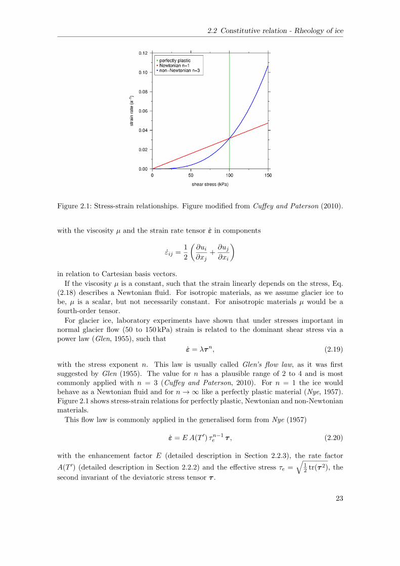
2.2 Constitutive relation - Rheology of ice
Figure 2.1: Stress-strain relationships. Figure modified from Cuffey and Paterson (2010).
with the viscosity µ and the strain rate tensor ε in components
εij =1
2
(
∂ui∂xj
+∂uj∂xi
)
in relation to Cartesian basis vectors.
If the viscosity µ is a constant, such that the strain linearly depends on the stress, Eq.(2.18) describes a Newtonian fluid. For isotropic materials, as we assume glacier ice tobe, µ is a scalar, but not necessarily constant. For anisotropic materials µ would be afourth-order tensor.
For glacier ice, laboratory experiments have shown that under stresses important innormal glacier flow (50 to 150 kPa) strain is related to the dominant shear stress via apower law (Glen, 1955), such that
ε = λτn, (2.19)
with the stress exponent n. This law is usually called Glen’s flow law, as it was firstsuggested by Glen (1955). The value for n has a plausible range of 2 to 4 and is mostcommonly applied with n = 3 (Cuffey and Paterson, 2010). For n = 1 the ice wouldbehave as a Newtonian fluid and for n→ ∞ like a perfectly plastic material (Nye, 1957).Figure 2.1 shows stress-strain relations for perfectly plastic, Newtonian and non-Newtonianmaterials.
This flow law is commonly applied in the generalised form from Nye (1957)
ε = E A(T ′) τn−1e τ , (2.20)
with the enhancement factor E (detailed description in Section 2.2.3), the rate factor
A(T ′) (detailed description in Section 2.2.2) and the effective stress τe =√
12 tr(τ
2), the
second invariant of the deviatoric stress tensor τ .
23
Chapter 2 Theory
To derive the inverse form of Eq. (2.20) the effective strain rate
εe =
√
1
2tr(ε2) (2.21)
is introduced, which is a scalar invariant of the strain rate tensor ε. By inserting Eq.(2.20) into Eq. (2.21), we derive
εe = E A(T ′) τn−1e τe ⇔ τe = [E A(T ′)]−1/n ε
1/ne . (2.22)
If we consider now again Eq. (2.18) and (2.20), the viscosity µ becomes
µ =1
2τ ε−1 =
1
2τ τ−1 [E A(T ′)]−1 τ1−n
e (2.23)
and can with Eq. (2.22) be written as
µ(T ′, εe) =1
2[E A(T ′)]−1/n ε
1−nn
e . (2.24)
Glacier ice has a high viscosity (µice ∼ 1 × 10¹³ Pa s at T ′ = 0C and τe = 100 kPa)compared to motor oil (µoil = 0.1Pa s) and a low viscosity compared to the mantle of theEarth (µearth ∼ 1× 10²¹ Pa s) (Greve and Blatter, 2009).
2.2.2 Rate factor
The rate factor A parametrises the influence of the temperature and the pressure on theviscosity and therefore the flow behaviour. The rate factor A increases exponentially withice temperature and the ice deforms much easier as it warms towards the pressure meltingpoint Tpmp. The higher deformation rate with increasing temperatures is mainly due tothe fact that creep processes are most effective when melting occurs at grain boundaries(Benn and Evans, 2010).
The rate factor can be described by the Arrhenius law (Cuffey and Paterson, 2010)
A(T, p) = A0e−(Q+pV )/RT (2.25)
with a pre-exponential constant A0, an activation energy for creep Q, the pressure p, an ac-tivation volume V , the universal gas constant R = 8.314 Jmol−1K−1 and the temperatureT .
For temperatures found in terrestrial ice, the value of A varies by a factor of 103 (Cuffeyand Paterson, 2010). For the pressure dependence of A, measurements have shown thatthe effect on the rate factor A is accounted for satisfactorily if the absolute temperatureT is replaced by the homologous temperature T ′ (refer to Eq. (2.17)) (Greve and Blatter,2009). The rate factor A can now be written as
A(T, p) = A(T ′) = A0e−Q/RT ′
. (2.26)
Paterson (1994) finds that for temperatures T < 263.15K = −10C the temperaturedependence of A is well described with constant values for A0 and Q. For temperaturesabove −10C, the ice softens more than would be predicted by the same values for A0
and Q. This might be due to grain-boundary sliding and the presence of liquid water on
24

2.2 Constitutive relation - Rheology of ice
the boundaries (Barnes et al., 1971). To achieve a continuous function for A with a stressexponent n = 3, the suggested values for A0 and Q are
A0 = 3.985× 10⁻¹³ s−1 Pa−3, Q = 60 kJmol−1 for T ′ ≤ 263.15K = −10C;A0 = 1.916× 10³ s−1 Pa−3, Q = 139 kJmol−1 for T ′ > 263.15K = −10C.
An alternative description for the temperature dependence of A often used in ice flowmodelling is given by Hooke (1981). For this study, we use the rate factor as suggested byPaterson (1994), because a comparison study shows that the parametrisation by Hooke(1981) can lead to unrealistic viscosity near the base (Payne and Baldwin, 2000).
The above stated relation has been established for ice below the pressure melting point,so called cold ice. Temperate ice is ice that is at pressure melting point Tpmp, and is inlocal equilibrium with its liquid phase (Lliboutry, 1971). Duval (1977) conducted creepexperiments with ice samples at pressure melting for a maximal water content of 0.8%,and found a linear relation, the strain rate tripled when the water content passes from lessthan 0.01 to 0.8%. These findings lay the basis for the introduction of a water contentdependent rate factor At. Following Lliboutry and Duval (1985), it can be chosen as
At(T, p,W ) = A(T, p) × (1 + 1.8125W [%]), (2.27)
with W being the water content, valid for W < 1%, being the rounded maximal valuefor the Duval relation (W < 0.8%). The water content can be explicitly calculated bysolving for the inner energy instead as for the temperature T (Aschwanden et al., 2012).Or the effect of the water content is approximated by assuming a water content of 1%, ifthe the temperature reaches the pressure melting point (e.g. Kleiner and Humbert, 2014).For temperatures < Tpmp, the rate factor for temperate ice At (Eq. 2.27) equals the ratefactor for cold ice A(T, p) (Eq. (2.26)). If used this way in the ice flow model, the maximalimpact of the water content onto the rate factor is simulated. A study of Pettersson et al.(2004) shows that the microscopic water content is generally < 3%.
2.2.3 Enhancement factor
There are a variety of factors that can influence the creep rate of glacier ice and which arenot captured by the rate factor A for cold ice. The creep rate can be influenced by thesize and orientation of crystals, the so called ice crystal fabric, inclusions of impurities,surface rifts or crevasses and water content (Budd and Jacka, 1989).The crystal c-axis orientation can lead to anisotropic behaviour, which is a preferred
direction of deformation (e.g. Gagliardini et al., 2009). On large scales the ice wouldappear softer in certain deformation directions. It is attempted to capture this effect byadjustment of the enhancement factor E. However, the introduction of E is somehow anadmission to the failure of the isotropy assumption used to formulate Glen’s flow law inthe first place. So far no real empirical relation was established between temperature,strain rate, cumulative strain and the enhancement factor E (Hooke, 2005). A variety oflaboratory experiments attempted to estimate values of E (e.g. Jacka and Budd, 1989;Dierckx and Tison, 2013), and result in a possible range E = [1, 10]. In general it can besaid, the higher the value for E, the softer the ice. Since there are other factors possiblysoftening the ice, attempts were made to link these to a value for E. Greve (1997), forexample, introduces an age dependent enhancement factor E, which parametrises thesoftening due to anisotropy and/or dust content. Also the large scale softening effect of
25

Chapter 2 Theory
surface rifts and crevasses can be parametrised by variation of E (Pralong, 2005; Humbert,2006).The enhancement factor E thus can account for all factors influencing the rheology of
the ice, that are not captured by the rate factor A. Cuffey and Paterson (2010) give adefinition of E such that
E =˙εmε, (2.28)
with a measured strain rate ˙εm and a calculated strain rate ε (Eq. (2.20)).The enhancement factor E can be seen in its origin as a somewhat physical parameter,
but is often used more as a tuning parameter, as its influence on the ice rheology can beattributed to a variety of factors. Most commonly a value of E = 1 is applied, but thereare several studies in which it increases by a factor of up to 103 (e.g. Echelmeyer, 1987).Such high values obtained in field studies might be due to errors in stress and temperatureestimates (Cuffey and Paterson, 2010). For shear margins in West Antarctic ice streams,a value as high as E = 12 has been inferred (Echelmeyer et al., 1994).
2.3 Overview of equations
The formulation of the balance equations for mass, momentum and energy in additionwith the constitutive relation give us a set of five equations to solve for the field quantitiesu, p, T of our interest (Reddy and Gartling, 2010). Here, for a better overview, we explicitlylist the equations solved for again.
Continuity equation
div(u) = 0,
Momentum equation
div(2µε− pI) = −ρg
with
µ =1
2[E A(T ′)]−1/n ε
1−n
ne .
Heat transfer equation
ρcp
(
∂T
∂t+ u grad T
)
= div(κ grad T ) + 4µε2e
2.4 Boundary conditions
The balance equations are defined under the assumption that the thermodynamic fieldsare sufficiently smooth, thus continuously differentiable. If this is not the case and aphysical quantity experiences a discontinuity across a surface, it is called a singular surface(Hutter and Johnk, 2004). The boundaries of the glacier are singular surfaces and thereforeadditional jump conditions, also called boundary conditions, have to be formulated. Aboundary condition can prescribe the derivative of the field quantity on the boundary andis then called a Neumann condition. If the value of the field quantity is known on the
26
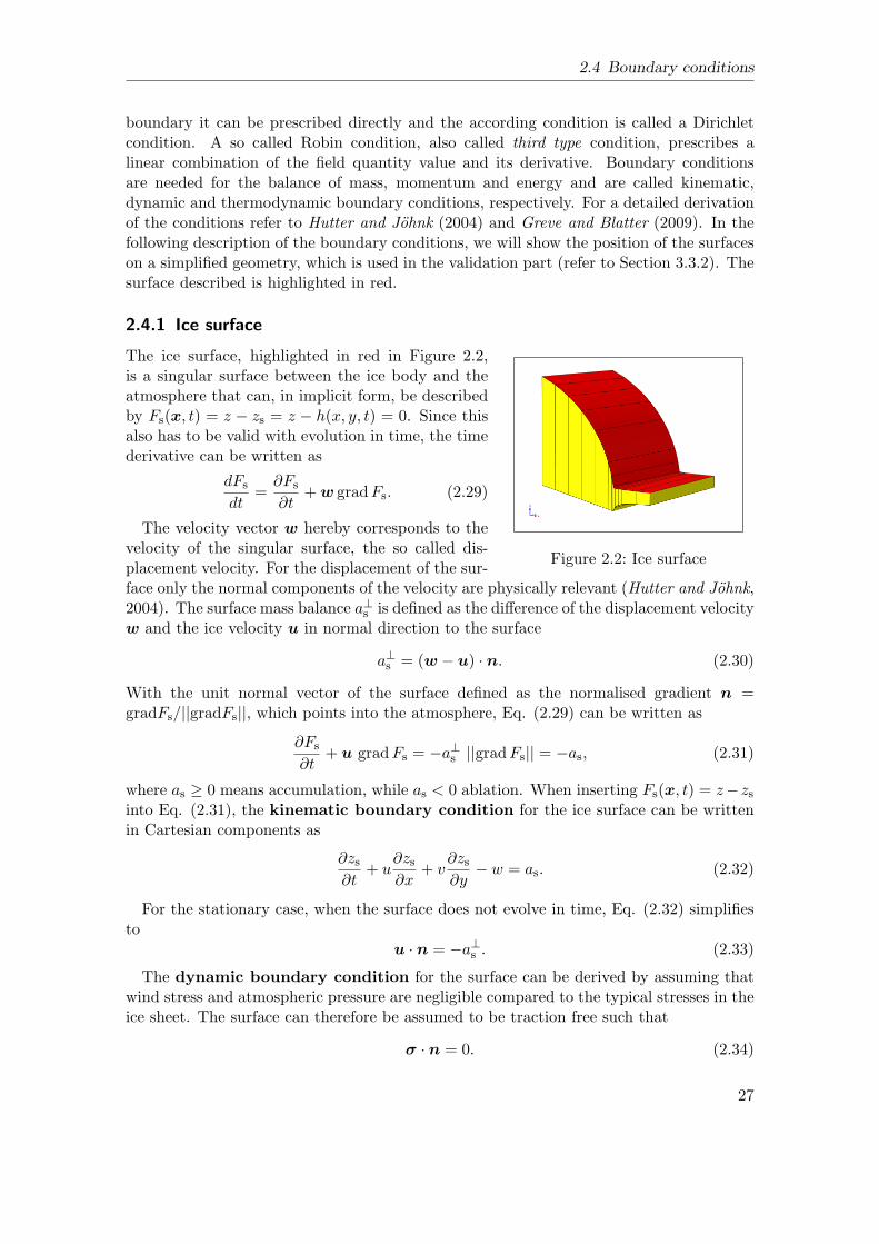
2.4 Boundary conditions
boundary it can be prescribed directly and the according condition is called a Dirichletcondition. A so called Robin condition, also called third type condition, prescribes alinear combination of the field quantity value and its derivative. Boundary conditionsare needed for the balance of mass, momentum and energy and are called kinematic,dynamic and thermodynamic boundary conditions, respectively. For a detailed derivationof the conditions refer to Hutter and Johnk (2004) and Greve and Blatter (2009). In thefollowing description of the boundary conditions, we will show the position of the surfaceson a simplified geometry, which is used in the validation part (refer to Section 3.3.2). Thesurface described is highlighted in red.
2.4.1 Ice surface
Figure 2.2: Ice surface
The ice surface, highlighted in red in Figure 2.2,is a singular surface between the ice body and theatmosphere that can, in implicit form, be describedby Fs(x, t) = z − zs = z − h(x, y, t) = 0. Since thisalso has to be valid with evolution in time, the timederivative can be written as
dFs
dt=∂Fs
∂t+w gradFs. (2.29)
The velocity vector w hereby corresponds to thevelocity of the singular surface, the so called dis-placement velocity. For the displacement of the sur-face only the normal components of the velocity are physically relevant (Hutter and Johnk,2004). The surface mass balance a⊥s is defined as the difference of the displacement velocityw and the ice velocity u in normal direction to the surface
a⊥s = (w − u) · n. (2.30)
With the unit normal vector of the surface defined as the normalised gradient n =gradFs/||gradFs||, which points into the atmosphere, Eq. (2.29) can be written as
∂Fs
∂t+ u gradFs = −a⊥s ||gradFs|| = −as, (2.31)
where as ≥ 0 means accumulation, while as < 0 ablation. When inserting Fs(x, t) = z−zsinto Eq. (2.31), the kinematic boundary condition for the ice surface can be writtenin Cartesian components as
∂zs∂t
+ u∂zs∂x
+ v∂zs∂y
− w = as. (2.32)
For the stationary case, when the surface does not evolve in time, Eq. (2.32) simplifiesto
u · n = −a⊥s . (2.33)
The dynamic boundary condition for the surface can be derived by assuming thatwind stress and atmospheric pressure are negligible compared to the typical stresses in theice sheet. The surface can therefore be assumed to be traction free such that
σ · n = 0. (2.34)
27
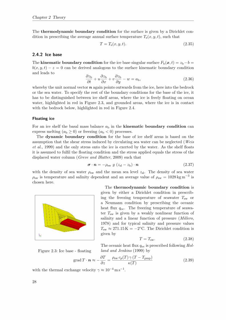
Chapter 2 Theory
The thermodynamic boundary condition for the surface is given by a Dirichlet con-dition in prescribing the average annual surface temperature Ts(x, y, t), such that
T = Ts(x, y, t). (2.35)
2.4.2 Ice base
The kinematic boundary condition for the ice base singular surface Fb(x, t) = zb−b =b(x, y, t) − z = 0 can be derived analogous to the surface kinematic boundary conditionand leads to
∂zb∂t
+ u∂zb∂x
+ v∂zb∂y
− w = ab, (2.36)
whereby the unit normal vector n again points outwards from the ice, here into the bedrockor the sea water. To specify the rest of the boundary conditions for the base of the ice, ithas to be distinguished between ice shelf areas, where the ice is freely floating on oceanwater, highlighted in red in Figure 2.3, and grounded areas, where the ice is in contactwith the bedrock below, highlighted in red in Figure 2.4.
Floating ice
For an ice shelf the basal mass balance ab in the kinematic boundary condition canexpress melting (ab ≥ 0) or freezing (ab < 0) processes.
The dynamic boundary condition for the base of ice shelf areas is based on theassumption that the shear stress induced by circulating sea water can be neglected (Weiset al., 1999) and the only stress onto the ice is exerted by the water. As the shelf floatsit is assumed to fulfil the floating condition and the stress applied equals the stress of thedisplaced water column (Greve and Blatter, 2009) such that
σ · n = −ρsw g (zsl − zb) · n (2.37)
with the density of sea water ρsw and the mean sea level zsl. The density of sea waterρsw is temperature and salinity dependent and an average value of ρsw = 1028 kgm−3 ischosen here.
Figure 2.3: Ice base - floating
The thermodynamic boundary condition isgiven by either a Dirichlet condition in prescrib-ing the freezing temperature of seawater Tsw ora Neumann condition by prescribing the oceanicheat flux qoc. The freezing temperature of seawa-ter Tsw is given by a weakly nonlinear function ofsalinity and a linear function of pressure (Millero,1978) and for typical salinity and pressure valuesTsw ≈ 271.15K = −2C. The Dirichlet condition isgiven by
T = Tsw. (2.38)
The oceanic heat flux qoc is prescribed following Hol-land and Jenkins (1999) by
gradT · n ≈ −∂T
∂z=ρsw cp(T ) γ (T − Tpmp)
κ(T )(2.39)
with the thermal exchange velocity γ ≈ 10−4ms−1.
28
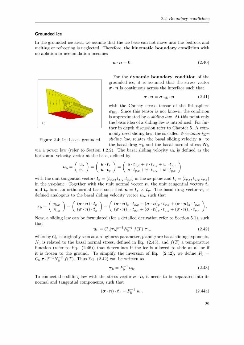
2.4 Boundary conditions
Grounded ice
In the grounded ice area, we assume that the ice base can not move into the bedrock andmelting or refreezing is neglected. Therefore, the kinematic boundary condition withno ablation or accumulation becomes
u · n = 0. (2.40)
Figure 2.4: Ice base - grounded
For the dynamic boundary condition of thegrounded ice, it is assumed that the stress vectorσ · n is continuous across the interface such that
σ · n = σlith · n (2.41)
with the Cauchy stress tensor of the lithosphereσlith. Since this tensor is not known, the conditionis approximated by a sliding law. At this point onlythe basic idea of a sliding law is introduced. For fur-ther in depth discussion refer to Chapter 5. A com-monly used sliding law, the so called Weertman-typesliding law, relates the basal sliding velocity ub tothe basal drag τ b and the basal normal stress Nb
via a power law (refer to Section 1.2.2). The basal sliding velocity ub is defined as thehorizontal velocity vector at the base, defined by
ub =
(
ubvb
)
=
(
u · txu · ty
)
=
(
u · tx,x + v · tx,y + w · tx,zu · ty,x + v · ty,y + w · ty,z
)
with the unit tangential vectors tx = (tx,x, tx,y, tx,z) in the xz-plane and ty = (ty,x, ty,y, ty,z)in the yz-plane. Together with the unit normal vector n, the unit tangential vectors txand ty form an orthonormal basis such that n = tx × ty. The basal drag vector τ b isdefined analogous to the basal sliding velocity vector ub, such that
τ b =
(
τb,xτb,y
)
=
(
(σ · n) · tx(σ · n) · ty
)
=
(
(σ · n)x · tx,x + (σ · n)y · tx,y + (σ · n)z · tx,z(σ · n)x · ty,x + (σ · n)y · ty,y + (σ · n)z · ty,z
)
.
Now, a sliding law can be formulated (for a detailed derivation refer to Section 5.1), suchthat
ub = Cb|τ b|p−1N−q
b f(T ) τ b, (2.42)
whereby Cb is originally seen as a roughness parameter, p and q are basal sliding exponents,Nb is related to the basal normal stress, defined in Eq. (2.45), and f(T ) a temperaturefunction (refer to Eq. (2.46)) that determines if the ice is allowed to slide at all or ifit is frozen to the ground. To simplify the inversion of Eq. (2.42), we define Fb =Cb|τ b|
p−1N−qb f(T ). Thus Eq. (2.42) can be written as
τ b = F−1b ub. (2.43)
To connect the sliding law with the stress vector σ · n, it needs to be separated into itsnormal and tangential components, such that
(σ · n) · tx = F−1b ub, (2.44a)
29
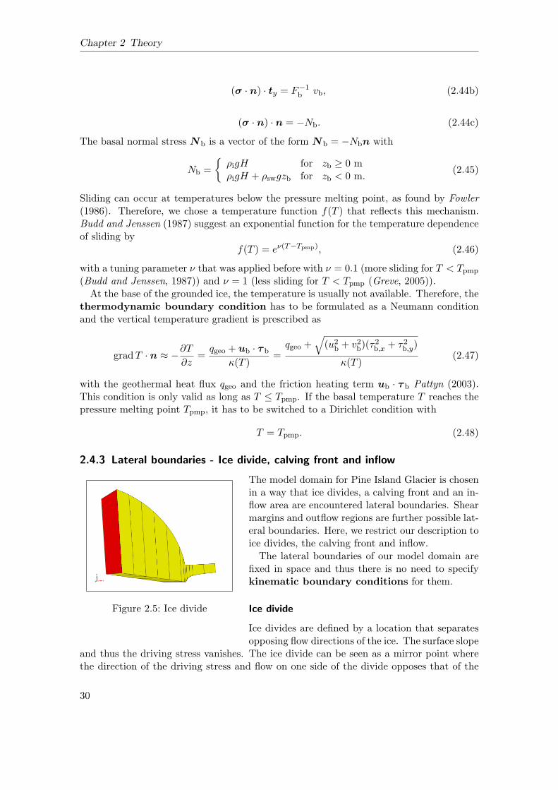
Chapter 2 Theory
(σ · n) · ty = F−1b vb, (2.44b)
(σ · n) · n = −Nb. (2.44c)
The basal normal stress Nb is a vector of the form Nb = −Nbn with
Nb =
ρigH for zb ≥ 0 mρigH + ρswgzb for zb < 0 m.
(2.45)
Sliding can occur at temperatures below the pressure melting point, as found by Fowler(1986). Therefore, we chose a temperature function f(T ) that reflects this mechanism.Budd and Jenssen (1987) suggest an exponential function for the temperature dependenceof sliding by
f(T ) = eν(T−Tpmp), (2.46)
with a tuning parameter ν that was applied before with ν = 0.1 (more sliding for T < Tpmp
(Budd and Jenssen, 1987)) and ν = 1 (less sliding for T < Tpmp (Greve, 2005)).At the base of the grounded ice, the temperature is usually not available. Therefore, the
thermodynamic boundary condition has to be formulated as a Neumann conditionand the vertical temperature gradient is prescribed as
gradT · n ≈ −∂T
∂z=qgeo + ub · τ b
κ(T )=qgeo +
√
(u2b + v2b)(τ2b,x + τ2b,y)
κ(T )(2.47)
with the geothermal heat flux qgeo and the friction heating term ub · τ b Pattyn (2003).This condition is only valid as long as T ≤ Tpmp. If the basal temperature T reaches thepressure melting point Tpmp, it has to be switched to a Dirichlet condition with
T = Tpmp. (2.48)
2.4.3 Lateral boundaries - Ice divide, calving front and inflow
Figure 2.5: Ice divide
The model domain for Pine Island Glacier is chosenin a way that ice divides, a calving front and an in-flow area are encountered lateral boundaries. Shearmargins and outflow regions are further possible lat-eral boundaries. Here, we restrict our description toice divides, the calving front and inflow.The lateral boundaries of our model domain are
fixed in space and thus there is no need to specifykinematic boundary conditions for them.
Ice divide
Ice divides are defined by a location that separatesopposing flow directions of the ice. The surface slope
and thus the driving stress vanishes. The ice divide can be seen as a mirror point wherethe direction of the driving stress and flow on one side of the divide opposes that of the
30

2.4 Boundary conditions
other side (Cuffey and Paterson, 2010). The lateral boundary coinciding with an ice divideis highlighted in red in Figure 2.5.The dynamic boundary condition for the ice divide is given by
(σ · n) · tx = 0 and (σ · n) · ty = 0 (2.49)
such that the tangential stresses vanish.The thermodynamic boundary condition for the ice divide is based on the assump-
tion that there is no temperature gradient across the divide. It can thus be written inform of a thermal insulation
(κ(T ) gradT ) · n = 0. (2.50)
Calving front
Figure 2.6: Calving front
The lateral boundary coinciding with the calvingfront is highlighted in red in Figure 2.6. The dy-namic boundary condition can be derived simi-lar to the one for the ice shelf base, such that
σ · n = −psw n (2.51)
with the only difference, that the pressure from thewater psw varies with depth and is defined as
psw =
0 for z ≥ zslρsw g (zsl − z) for z < zsl
(2.52)
The thermodynamic boundary condition for the calving front is given by thermalinsulation as in Eq. (2.50).
Inflow
The dynamic boundary condition is given as a Dirichlet condition by an inflow velocityfield uSIA = (uSIA, vSIA, wSIA) defined with the Shallow Ice Approximation SIA (refer toSection 1.2.1). The horizontal velocity components uSIA and vSIA are given by
uSIA(z) = ub,SIA − 2(ρg)n|grad zs|n−1
(
∂zs∂x
)
∫ z
zb
A(zs − z)ndz,
vSIA(z) = vb,SIA − 2(ρg)n|grad zs|n−1
(
∂zs∂y
)
∫ z
zb
A(zs − z)ndz,(2.53)
with
|grad zs| =
√
(
∂zs∂x
)2
+
(
∂zs∂y
)2
and∫ z
zb
A(zs − z)ndz =A
n+ 1((zs − zb)
n+1 − (zs − z)n+1).
The basal velocity components ub,SIA and vb,SIA are assumed to be zero, as is the verticalvelocity component wSIA. The rate factor A is here taken as a constant value A = const. =
31
Chapter 2 Theory
1e − 25, which corresponds to a constant temperature T ∼ −25C (Greve and Blatter,2009).The thermodynamic boundary condition for the inflow is given by a linear tem-
perature profile
Tlin =Tpmp − Tszs − zb
(zs − z) + Ts. (2.54)
2.5 Finite element method - FEM
The Finite Element Method (FEM) is a numerical method for finding approximate solu-tions to Partial Differential Equations (PDE). Numerical methods are for example neededwhen it is not possible to find an analytical solution to a problem, which is the case forthe Navier-Stokes equations. Another commonly applied numerical method is the Fi-nite Difference Method (FDM). Here we introduce the FEM, and when helpful for theunderstanding, highlight the difference to the FDM.We introduce the FEM along a simple 1D problem, the 1D Poisson equation, which is
an elliptic second-order PDE. The description in this section is based on Hughes (2000),Reddy and Gartling (2010) and Johnson (2009). We attempt to find a balance betweenmathematical elaboration and comprehensive description.The 1D Poisson equation, defined on the domain Ω = [0, 1] with the boundaries ∂Ω =
0, 1, is given by
f(x) = −∂2u
∂x2on Ω, (2.55)
with uniform Dirichlet boundary conditions
u = 0 on ∂Ω, (2.56)
for which we aim to find a solution u.Solving a PDE numerically requires partitioning of the domain Ω into small units of a
simple shape, the mesh elements. The process is called discretization or meshing of thedomain, and is described in Section 2.5.1. On these mesh elements the physical field, inour example u, is approximated by simpler functions, the approximation or basis functions,described in Section 2.5.2. While the FDM is based on the original PDE, the FEM is basedon a weighted-integral form of the PDE, which is introduced in Section 2.5.3. This is animportant feature, giving the FEM higher flexibility in problem application. In Section2.5.4 a few remarks about boundary conditions are made. The approximated fields needto be assembled into a global system of algebraic equations for the entire domain Ω,described in Section 2.5.5. And finally, to obtain a solution, the assembled matrix, the socalled coefficient matrix, needs to be solved, described in Section 2.5.6.
2.5.1 Meshing
Most numerical methods have in common, that the domain Ω, on which the PDE isaimed to be solved, needs to be divided into small units of a simple shape, the so calledmesh elements Ωe, with the element boundaries ∂Ωe. The entire mesh Ωh consists of thenon-overlapping sum of all elements, such that
Ωh = ∪Ωe. (2.57)
32

2.5 Finite element method - FEM
For complex geometries the mesh Ωh may not exactly equal the total domain Ω.In the FEM the mesh elements Ωe are not required to be equal sized and thus non-
uniform meshes can be used. Additionally a variety of geometric shapes can be chosen.However, the choice of element shape is subject to certain conditions. For conformingelements, which are described here, neighbouring elements for example are required toshare nodes. And the approximation functions, described in the next section, are requiredto be uniquely derivable for the elements. Still, a FEM mesh can conveniently be appliedto complex geometries and refined in regions of interest, which could be regions with largegradients in the solution. An example of a FEM mesh is shown in Figure 2.7.
Figure 2.7: Example of a non-uniform FEM mesh on a complex geometry
In our 1D example we divide our domain Ω = [0, 1] into two equal sized elements, whichare described as mesh intervals 0 < x < 0.5 and 0.5 < x < 1. The element or mesh nodesxj are in this 1D example the boundaries of the elements, such that x1 = 0, x2 = 0.5 andx3 = 1.
2.5.2 Approximation functions - Basis functions
To approach the solution u by an approximate solution u on the domain Ω, we defineapproximation functions Nj , such that
u(x) ≈ u(x) =n∑
j=1
Nj(x)ue(xj), (2.58)
where Nj are linearly independent functions, and uej = ue(xj) the still unknown valuesof u at the mesh nodes xj , which are discrete points in the domain. This is a so calledGalerkin approximation.
The approximation functions Nj are also known as basis functions. When these functionsare defined only over a reference element, and described in terms of element coordinates,which are local coordinates related to a uniform element shape, they are also called shapefunctions, because they assume one of a few basic shapes. In the subsequent descriptionwe will refer to the Nj as basis functions.
All basis functions are defined over the entire domain. The most common type arecalled Lagrange basis functions and required to be Nj = 1 at node xj and zero on all
33

Chapter 2 Theory
Figure 2.8: Linear basis functions N1
and N2
Figure 2.9: Quadratic basis functionsN1, N2 and N3
other nodes. The quality of the solution depends on how well the basis functions Nj
can approximate the solution of the PDE. The simplest conforming basis functions arelinear and can be seen in Figure 2.8 over the first element 0 < x < 0.5. Quadraticbasis functions require another node in the middle of the 1D element and are shown inFigure 2.9 over the same element. The accuracy of the solution depends on the resolutionof the underlying mesh and the choice of basis functions. A finer mesh results in morenodes on which the approximate solutions are found, while a higher order basis functionleads to better approximation between the nodal values. It can be proven in a generalform that the approximation error |u − u| ≤ Chq, where u is the exact solution, u thediscrete approximate solution, C a problem dependent constant, h the mesh size and qthe polynomial order of the Lagrange basis function.
The phrase finite element refers to the geometry of the element plus the shape functionson the element. The mesh items alone are referred to as mesh elements or cells. Differentchoices of shape functions can define different types of finite elements. One type of finiteelements are Lagrange elements, which are described here. Other finite elements areBubble elements, Curl elements or Discontinuous elements, which are not described herein more detail.
2.5.3 Weighted-integral form
The method is based on a weighted-integral form of the PDE to be solved, given in Eq.(2.55). A weighted-integral form of a PDE can be obtained with the variational formu-lation. The resulting weighted-integral statement is equivalent to the governing PDE andsometimes referred to as the global weak form, which is different to the weak form of theweighted-integral statement and will be made clear below. The existence and uniquenessof the solution of the weak form can be shown with the Lax-Milgram theorem, but willnot be further discussed here.
A weight function wi is chosen, with which the original PDE (Eq. (2.55)) is multipliedon both sides, and integrated over the domain Ω, such that for every choice of wi
∫
Ωf wi dx =
∫
Ω
(
−∂2u
∂x2
)
wi dx. (2.59)
The weight functions wi are also called trial or test functions.
34
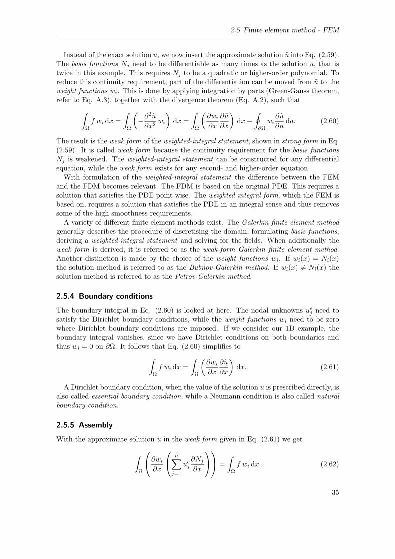
2.5 Finite element method - FEM
Instead of the exact solution u, we now insert the approximate solution u into Eq. (2.59).The basis functions Nj need to be differentiable as many times as the solution u, that istwice in this example. This requires Nj to be a quadratic or higher-order polynomial. Toreduce this continuity requirement, part of the differentiation can be moved from u to theweight functions wi. This is done by applying integration by parts (Green-Gauss theorem,refer to Eq. A.3), together with the divergence theorem (Eq. A.2), such that
∫
Ωf wi dx =
∫
Ω
(
−∂2u
∂x2wi
)
dx =
∫
Ω
(
∂wi
∂x
∂u
∂x
)
dx−
∮
∂Ωwi∂u
∂nda. (2.60)
The result is the weak form of the weighted-integral statement, shown in strong form in Eq.(2.59). It is called weak form because the continuity requirement for the basis functionsNj is weakened. The weighted-integral statement can be constructed for any differentialequation, while the weak form exists for any second- and higher-order equation.
With formulation of the weighted-integral statement the difference between the FEMand the FDM becomes relevant. The FDM is based on the original PDE. This requires asolution that satisfies the PDE point wise. The weighted-integral form, which the FEM isbased on, requires a solution that satisfies the PDE in an integral sense and thus removessome of the high smoothness requirements.
A variety of different finite element methods exist. The Galerkin finite element methodgenerally describes the procedure of discretising the domain, formulating basis functions,deriving a weighted-integral statement and solving for the fields. When additionally theweak form is derived, it is referred to as the weak-form Galerkin finite element method.Another distinction is made by the choice of the weight functions wi. If wi(x) = Ni(x)the solution method is referred to as the Bubnov-Galerkin method. If wi(x) 6= Ni(x) thesolution method is referred to as the Petrov-Galerkin method.
2.5.4 Boundary conditions
The boundary integral in Eq. (2.60) is looked at here. The nodal unknowns uej need tosatisfy the Dirichlet boundary conditions, while the weight functions wi need to be zerowhere Dirichlet boundary conditions are imposed. If we consider our 1D example, theboundary integral vanishes, since we have Dirichlet conditions on both boundaries andthus wi = 0 on ∂Ω. It follows that Eq. (2.60) simplifies to
∫
Ωf wi dx =
∫
Ω
(
∂wi
∂x
∂u
∂x
)
dx. (2.61)
A Dirichlet boundary condition, when the value of the solution u is prescribed directly, isalso called essential boundary condition, while a Neumann condition is also called naturalboundary condition.
2.5.5 Assembly
With the approximate solution u in the weak form given in Eq. (2.61) we get
∫
Ω
∂wi
∂x
n∑
j=1
uej∂Nj
∂x
=
∫
Ωf wi dx. (2.62)
35

Chapter 2 Theory
Every choice of the weight functions wi gives an algebraic relation between the nodalunknowns uj . Thus m linearly independent choices of wi lead to m linearly independentalgebraic equations. Here we describe the Bubnov-Galerkin method with wi(x) = Ni(x)and can therefore write
n∑
j=1
∫
Ω
(
∂Ni
∂x
∂Nj
∂xdx
)
uej =
∫
ΩfNi dx. (2.63)
Eq. (2.63) represents a system of n equations for n unknowns and can be written inmatrix form. To do so we define
n∑
j=1
Ki,j uej = Fi (2.64)
with
Ki,j =
∫
Ω
∂Ni
∂x
∂Nj
∂xdx (2.65)
and
Fi =
∫
ΩfNi dx (2.66)
Ki,j are the single entries of the coefficient matrix K and Fi the single entries of the forcevector F . With the elements uej of the solution vector u, the matrix form can be writtenas
Ku = F . (2.67)
The nodal unknowns uej and the Dirichlet boundary conditions are the entries in thesolution vector u, while the Neumann boundary conditions are included in the force vectorF .When assembling the coefficient matrix K, continuity of the nodal unknowns uej and
balance of the derivatives on neighbouring elements have to be considered.The number of entries n in the solution vector u are the so called Degrees Of Freedom
(DOF).
2.5.6 Solution
This system of linear algebraic equations given in Eq. (2.67) now needs to be solved foru, such that
u = K−1F . (2.68)
Most of the entries in the coefficient matrix Ki,j are zero, as the basis and weight functionsNi are defined to only be 6= 0 on single nodes and its surroundings, as shown in Section2.5.2. Thus, depending on the choice of Ni, the coefficient matrix K can be a sparsematrix, whose non-zero entries are confined to the main diagonal, or some more diagonalson either side.The coefficient matrix K may be either symmetric, as in this example, or unsymmetric,
depending on the underlying PDE. When considering bigger matrices that have to besolved computationally, the above mentioned characteristics of the coefficient matrix K
are very important for choosing an appropriate matrix solution procedure. The solutioncan be found by either a direct or iterative method. Direct methods, based on the Gauss
36

2.5 Finite element method - FEM
elimination technique, provide the solution after a fixed number of steps and are lesssensitive to the conditioning of the coefficient matrix K, but they are not practical forlarge numbers of DOFs due to high computational cost. Iterative methods do not need toform the global matrix as in the direct method and are therefore computationally cheaperand can more easily be parallelized, but they are more difficult to apply if the system isnot well-conditioned.
37

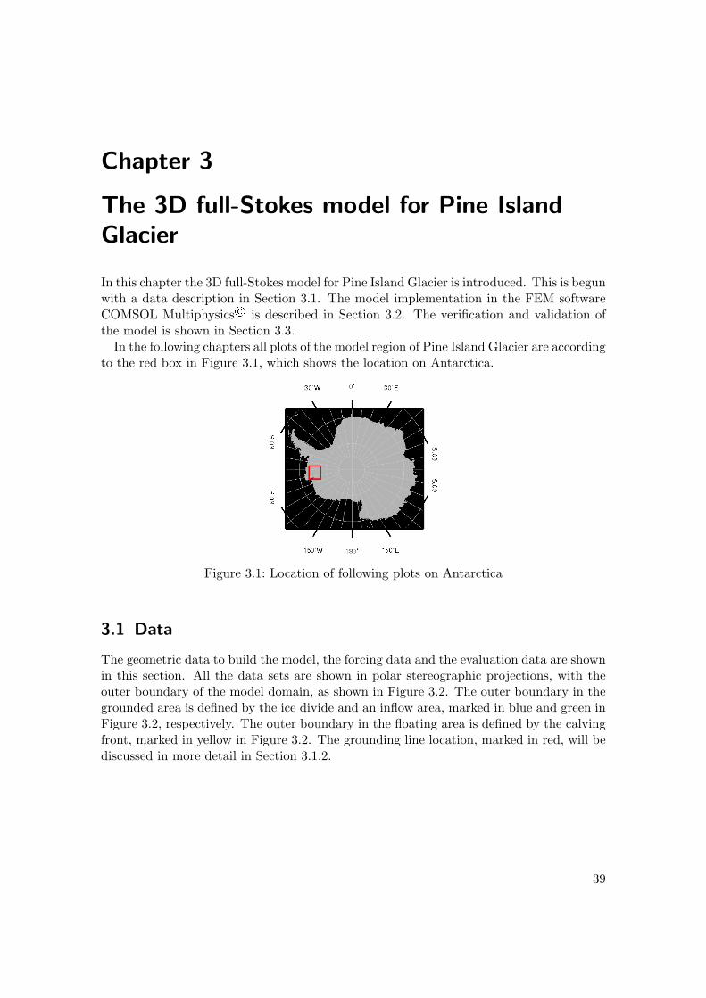
Chapter 3
The 3D full-Stokes model for Pine Island
Glacier
In this chapter the 3D full-Stokes model for Pine Island Glacier is introduced. This is begunwith a data description in Section 3.1. The model implementation in the FEM softwareCOMSOL Multiphysics© is described in Section 3.2. The verification and validation ofthe model is shown in Section 3.3.
In the following chapters all plots of the model region of Pine Island Glacier are accordingto the red box in Figure 3.1, which shows the location on Antarctica.
Figure 3.1: Location of following plots on Antarctica
3.1 Data
The geometric data to build the model, the forcing data and the evaluation data are shownin this section. All the data sets are shown in polar stereographic projections, with theouter boundary of the model domain, as shown in Figure 3.2. The outer boundary in thegrounded area is defined by the ice divide and an inflow area, marked in blue and green inFigure 3.2, respectively. The outer boundary in the floating area is defined by the calvingfront, marked in yellow in Figure 3.2. The grounding line location, marked in red, will bediscussed in more detail in Section 3.1.2.
39
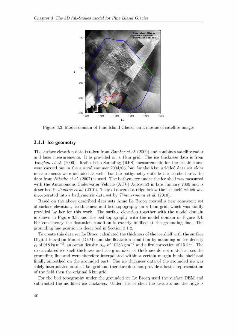

3.1 Data
Figure 3.3: Surface elevation Figure 3.4: Bed topography
incorporated from Timmermann et al. (2010) and the rest is interpolated, but still makingsure no unrealistic shallow areas develop where the ice shelf would ground.
This data set finally represents the thickness distribution of Pine Island Glacier for theyear 2005 and earlier. A lot of new thickness measurements have been conducted in thearea during the Ice Bridge Campaign in the years 2009, 2010 and 2011. This thicknessdata is not yet incorporated.
3.1.2 Grounding line position
The GRounding Line (GRL) position used in the diagnostic model is given by a combi-nation of the positions in the MODIS (MODerate-resolution Imaging Spectroradiometer)Mosaic Of Antarctica (MOA) (Bohlander and Scambos, 2007) (corresponding to the years2003/2004), the position in Rignot (1998) (corresponding to 1996) and the position thatgives the smoothest ice thickness join of the procedure described above, all shown in Figure3.5. This combination was chosen because there is no single source to describe the locationbest. Though the MOA grounding line position corresponds to the years 2003/2004, itshows unrealistic retreat in the central trough area, as shown in red in Figure 3.5. For thecentral trough area grounding line location estimates exist for the years 1992, 1994, 1996(yellow in Figure 3.5) (all Rignot, 1998), 2000 (Rignot, 2002), 2003/2004 (red in Figure3.5) (Bohlander and Scambos, 2007), 2007 (Rignot, 2008) and 2009 (blue in Figure 3.5)(Joughin et al., 2010). The procedures to derive these positions differ in their accuracy.
The 1992 and 1994 positions were determined with InSAR (Interferometric SyntheticAperture Radar) from the ERS-1 (European Remote Sensing) Satellite. The repeat pe-riods between the acquisitions for 1992 and 1994 are 6 and 3 days respectively (Rignot,1998). The 1996 and 2000 positions were determined with InSAR using the ERS tandemacquisitions, with a repeat period of 1 day. The ERS tandem mission ended in 2000 andwith this for the time being the ability to measure grounding-line positions on Pine IslandGlacier in high accuracy, as the repeat periods of other radar satellites were much toolarge. A too large repeat period (>> 1 day) produces interferometric phases that are too
41

3.1 Data
The two rifted regions eventually merged and the ice shelf was not grounded on the icerise any longer.
3.1.4 Surface temperature
Figure 3.6: Surface temperature Ts,obs
The data set used here is on a 5 km grid compiled by Le Brocq et al. (2010) (ALBMAPv1), based on the temperature data described in Comiso (2000). The surface temperatureis estimated from Advanced Very High Resolution Radiometer (AVHRR) infrared data.Annual mean temperatures from 1982 to 2004 were averaged for the temperature fieldshown in Figure 3.6 (Le Brocq et al., 2010). The annual mean temperature shows notemperatures near the melting point, but in the annual cycle surface melting is occasionallypresent in the lower regions and on the ice shelf. The lowest temperatures are found onthe highest elevated surface and increase towards the shelf, where the high heat capacityof the ocean water lead to the lowest annual temperatures.
3.1.5 Geothermal heat flux
The geothermal heat flux qgeo varies spatially because it depends on local geologic con-ditions such as the tectonic history of the crust, heat production within the crust dueto decay of radioactive isotopes and the mantle heat flux. The global average heat fluxis estimated to be about 0.06Wm−2 and is enough to melt 6mm of ice at its pressuremelting point each year (Cuffey and Paterson, 2010). Due to the distinct geologic historyof West and East Antarctica (refer to Section 1.1.1), the geothermal heat flux in WestAntarctica is expected to be nearly three times higher than in East Antarctica and muchmore variable (Shapiro and Ritzwoller, 2004). Therefore especially in West Antarcticathe geothermal heat flux is an important component when modelling ice dynamics. The
43
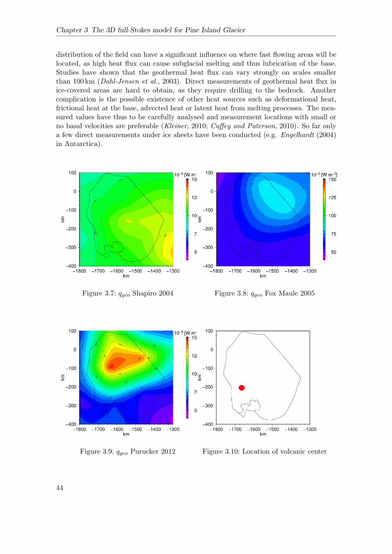
Chapter 3 The 3D full-Stokes model for Pine Island Glacier
distribution of the field can have a significant influence on where fast flowing areas will belocated, as high heat flux can cause subglacial melting and thus lubrication of the base.Studies have shown that the geothermal heat flux can vary strongly on scales smallerthan 100 km (Dahl-Jensen et al., 2003). Direct measurements of geothermal heat flux inice-covered areas are hard to obtain, as they require drilling to the bedrock. Anothercomplication is the possible existence of other heat sources such as deformational heat,frictional heat at the base, advected heat or latent heat from melting processes. The mea-sured values have thus to be carefully analysed and measurement locations with small orno basal velocities are preferable (Kleiner, 2010; Cuffey and Paterson, 2010). So far onlya few direct measurements under ice sheets have been conducted (e.g. Engelhardt (2004)in Antarctica).
Figure 3.7: qgeo Shapiro 2004 Figure 3.8: qgeo Fox Maule 2005
Figure 3.9: qgeo Purucker 2012 Figure 3.10: Location of volcanic center
44
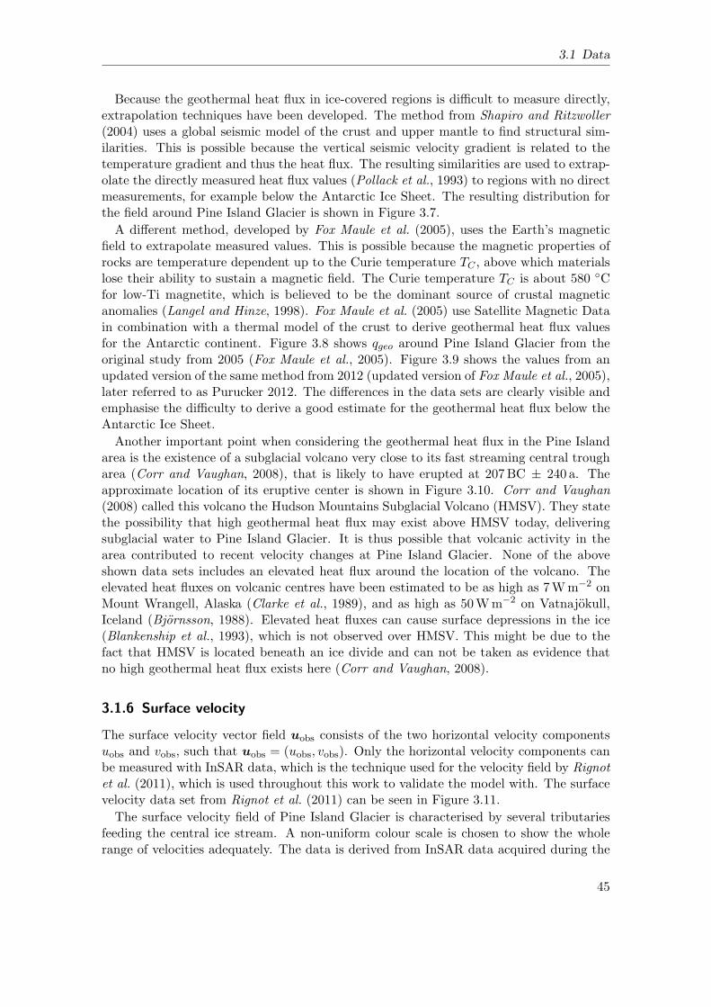
3.1 Data
Because the geothermal heat flux in ice-covered regions is difficult to measure directly,extrapolation techniques have been developed. The method from Shapiro and Ritzwoller(2004) uses a global seismic model of the crust and upper mantle to find structural sim-ilarities. This is possible because the vertical seismic velocity gradient is related to thetemperature gradient and thus the heat flux. The resulting similarities are used to extrap-olate the directly measured heat flux values (Pollack et al., 1993) to regions with no directmeasurements, for example below the Antarctic Ice Sheet. The resulting distribution forthe field around Pine Island Glacier is shown in Figure 3.7.
A different method, developed by Fox Maule et al. (2005), uses the Earth’s magneticfield to extrapolate measured values. This is possible because the magnetic properties ofrocks are temperature dependent up to the Curie temperature TC , above which materialslose their ability to sustain a magnetic field. The Curie temperature TC is about 580 Cfor low-Ti magnetite, which is believed to be the dominant source of crustal magneticanomalies (Langel and Hinze, 1998). Fox Maule et al. (2005) use Satellite Magnetic Datain combination with a thermal model of the crust to derive geothermal heat flux valuesfor the Antarctic continent. Figure 3.8 shows qgeo around Pine Island Glacier from theoriginal study from 2005 (Fox Maule et al., 2005). Figure 3.9 shows the values from anupdated version of the same method from 2012 (updated version of Fox Maule et al., 2005),later referred to as Purucker 2012. The differences in the data sets are clearly visible andemphasise the difficulty to derive a good estimate for the geothermal heat flux below theAntarctic Ice Sheet.
Another important point when considering the geothermal heat flux in the Pine Islandarea is the existence of a subglacial volcano very close to its fast streaming central trougharea (Corr and Vaughan, 2008), that is likely to have erupted at 207BC ± 240 a. Theapproximate location of its eruptive center is shown in Figure 3.10. Corr and Vaughan(2008) called this volcano the Hudson Mountains Subglacial Volcano (HMSV). They statethe possibility that high geothermal heat flux may exist above HMSV today, deliveringsubglacial water to Pine Island Glacier. It is thus possible that volcanic activity in thearea contributed to recent velocity changes at Pine Island Glacier. None of the aboveshown data sets includes an elevated heat flux around the location of the volcano. Theelevated heat fluxes on volcanic centres have been estimated to be as high as 7Wm−2 onMount Wrangell, Alaska (Clarke et al., 1989), and as high as 50Wm−2 on Vatnajokull,Iceland (Bjornsson, 1988). Elevated heat fluxes can cause surface depressions in the ice(Blankenship et al., 1993), which is not observed over HMSV. This might be due to thefact that HMSV is located beneath an ice divide and can not be taken as evidence thatno high geothermal heat flux exists here (Corr and Vaughan, 2008).
3.1.6 Surface velocity
The surface velocity vector field uobs consists of the two horizontal velocity componentsuobs and vobs, such that uobs = (uobs, vobs). Only the horizontal velocity components canbe measured with InSAR data, which is the technique used for the velocity field by Rignotet al. (2011), which is used throughout this work to validate the model with. The surfacevelocity data set from Rignot et al. (2011) can be seen in Figure 3.11.
The surface velocity field of Pine Island Glacier is characterised by several tributariesfeeding the central ice stream. A non-uniform colour scale is chosen to show the wholerange of velocities adequately. The data is derived from InSAR data acquired during the
45

Chapter 3 The 3D full-Stokes model for Pine Island Glacier
Figure 3.11: Surface Velocity |uobs| with normed vector field uobs
years 2007 to 2009. The area, where the outer boundary does not coincide with the icedivide but an inflow, can be seen.
The main flow direction in the central trough is towards the west, where the ice shelf islocated. To the north of the ice shelf two smaller ice streams, and to the south one smalland fast stream, can be seen.
3.2 Implementation
The 3D full-Stokes model for the flow of Pine Island Glacier is set up with the commercialFinite Element Method software COMSOL Multiphysics©. The FEM is a numericaltechnique (for details refer to Section 2.5) for finding approximate solutions to partialdifferential equations, which form the basis for most physical laws. COMSOL providesan environment where complex 3D FEM models can be created without the need for anin-depth knowledge of mathematics or numerical analysis. On the other hand, because itis a commercial software, it is not possible to access the actual source code.
The application of COMSOL Multiphysics© for ice dynamic simulations will be referredto as the model COMice in the subsequent description.
To set up a model with COMSOL a Graphical User Interface (GUI) is provided, ascreenshot of which is shown in Figure 3.12. This is very convenient to start of withand try new settings, but not needed any longer once the model is set up and running.Additionally, with the so called COMSOL LiveLink for MATLAB, it is possible to usescript programming in Java (COMSOL API (Application Programming Interface) Java)or the MATLAB language, to set up and modify a model. To solve the model COMSOLinternally compiles a set of equations representing the entire model.
The following GUI description is based on COMSOL version 4.3a. The COMSOL GUIconsists primarily of the Model Builder, Node Settings, and Graphics windows. The Model
46
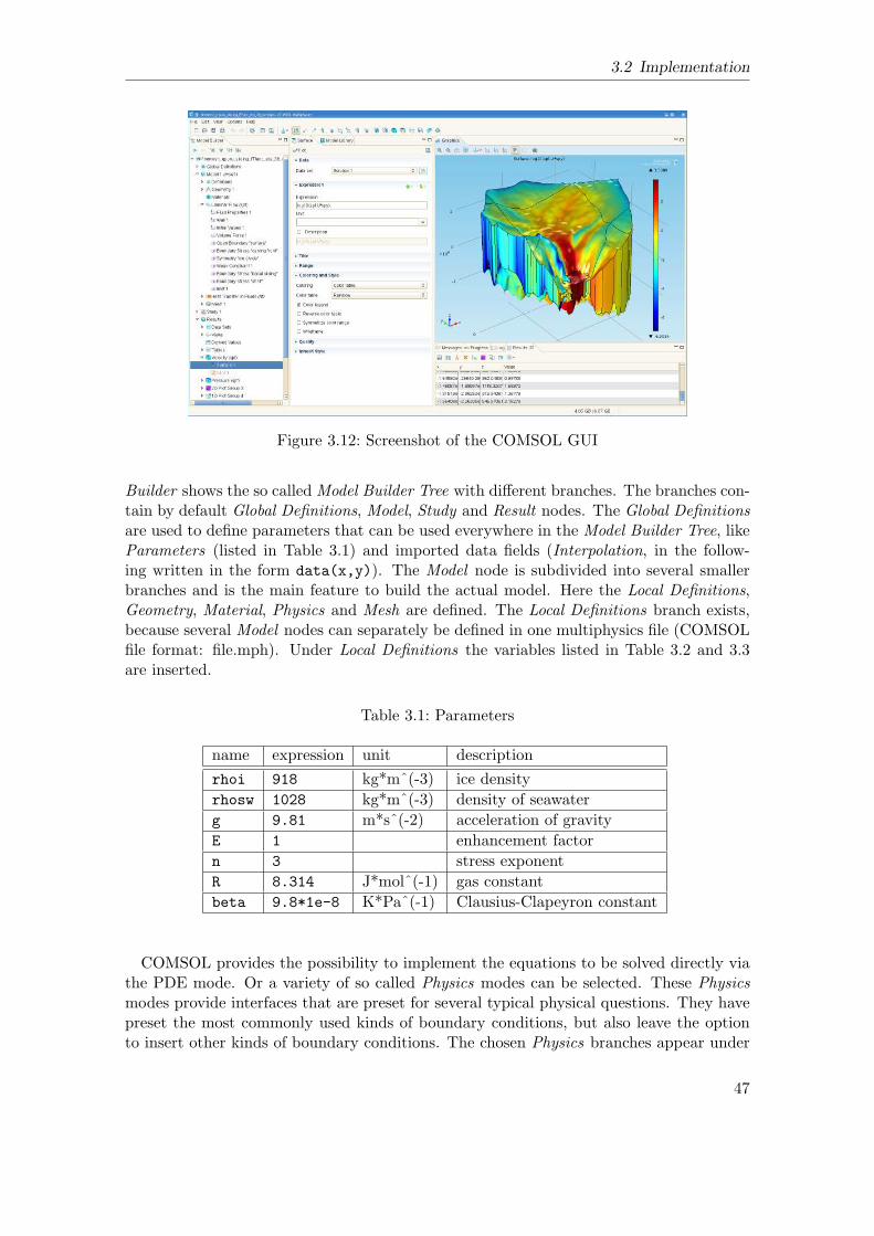
3.2 Implementation
Figure 3.12: Screenshot of the COMSOL GUI
Builder shows the so called Model Builder Tree with different branches. The branches con-tain by default Global Definitions, Model, Study and Result nodes. The Global Definitionsare used to define parameters that can be used everywhere in the Model Builder Tree, likeParameters (listed in Table 3.1) and imported data fields (Interpolation, in the follow-ing written in the form data(x,y)). The Model node is subdivided into several smallerbranches and is the main feature to build the actual model. Here the Local Definitions,Geometry, Material, Physics and Mesh are defined. The Local Definitions branch exists,because several Model nodes can separately be defined in one multiphysics file (COMSOLfile format: file.mph). Under Local Definitions the variables listed in Table 3.2 and 3.3are inserted.
Table 3.1: Parameters
name expression unit description
rhoi 918 kg*mˆ(-3) ice density
rhosw 1028 kg*mˆ(-3) density of seawater
g 9.81 m*sˆ(-2) acceleration of gravity
E 1 enhancement factor
n 3 stress exponent
R 8.314 J*molˆ(-1) gas constant
beta 9.8*1e-8 K*Paˆ(-1) Clausius-Clapeyron constant
COMSOL provides the possibility to implement the equations to be solved directly viathe PDE mode. Or a variety of so called Physics modes can be selected. These Physicsmodes provide interfaces that are preset for several typical physical questions. They havepreset the most commonly used kinds of boundary conditions, but also leave the optionto insert other kinds of boundary conditions. The chosen Physics branches appear under
47

Chapter 3 The 3D full-Stokes model for Pine Island Glacier
Physics in the Model Builder Tree. To simulate the Stokes flow the Physics mode LaminarFlow is selected, which provides the Navier-Stokes equation. The temperature is solvedfor with the Physics mode Heat Transfer in Fluids, which provides the heat transportequation. How the boundary conditions are implemented in the Physics modes will bedescribed below.
In the following sections it is explained how the geometry is built (Section 3.2.1), howthe Laminar Flow (Section 3.2.2) and Heat Transfer in Fluids (Section 3.2.3) modes withappropriate boundary conditions are applied, how the mesh is created (Section 3.2.4) andwhich solvers are selected (Section 3.2.5). This is done by describing the path to followin italic characters. The actual input that needs to be done is written in typewrite
characters and further specifications if needed can be found in Tables 3.1, 3.2 and 3.3.
3.2.1 Model geometry
The geometry in a COMSOL model is the central object. For a glacier model it has to becreated as a solid, the so called Model Domain. This main Model Domain can be dividedinto a variety of Model Subdomains, which will become important for defining differentboundary conditions or mesh resolutions.
The basic idea to create a realistic model geometry based on topographic data is tofirst create the horizontal domain boundary, possibly including horizontal subdomains.For Pine Island Glacier the outer domain boundaries are described in Section 3.1 andshown in Figure 3.2. The ice shelf area represents hereby a subdomain, separated by thegrounding line position from the grounded ice. This flat xy-plane is next extruded inz-direction to create a 3D object. The gridded topographic data of the upper and lowersurfaces have to be converted into solid interpolated 3D COMSOL surfaces. To receivethe final 3D object, the extruded 3D object has to be cut with the two surfaces.
COMSOL version 4.3a provides in theory functionalities to conduct the above describedsteps. The interpolated 3D COMSOL surfaces are created with the function parametricsurface. Unfortunately this functionality seems to be only practical for smaller geometries,where deviations (due to smoothing) from the input data do not matter greatly. Thetopographic input data for Pine Island Glacier is in high resolution and consists for theupper and lower surfaces of a 1 km mesh for an area roughly 1000 x 500 km2. The surfaceshave to be represented as exact as possible, since otherwise for example the position ofthe grounding line might change. When the geometry is set up completely in version 4.3a,the resulting COMSOL file becomes huge and impractical to work with.
Therefore, the model geometry was built with the help of version 3.5a and the COMSOLLiveLink for MATLAB. In version 3.5a the COMSOL function geomsurf is available, whichcreates solid interpolated 3D COMSOL surfaces. The so created surfaces use a lot lessmemory and are thus more practical to work with. Unfortunately this function is notavailable in later versions. A quadratic interpolation is used to create a surface withparametric surface (COMSOL, 2012a, p.707), while geomsurf uses a piecewise quadraticinterpolation on a triangular mesh (COMSOL, 2008, p.275).
The geometry is built in MATLAB with COMSOL version 3.5a, saved as a geometryobject and imported into COMSOL version 4.3a. To represent and work with complex 3Dgeometries, like the Pine Island Glacier geometry, the CAD Import module for COMSOL4.3a is required. This module has its own geometry kernel (Parasolid). With this modulearbitrary lines can be cut through the 3D geometry and thus new subdomains can be
48
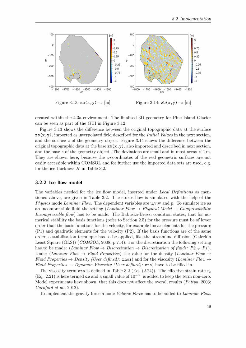
3.2 Implementation
Figure 3.13: zs(x,y)−z [m] Figure 3.14: zb(x,y)−z [m]
created within the 4.3a environment. The finalised 3D geometry for Pine Island Glaciercan be seen as part of the GUI in Figure 3.12.
Figure 3.13 shows the difference between the original topographic data at the surfacezs(x,y), imported as interpolated field described for the Initial Values in the next section,and the surface z of the geometry object. Figure 3.14 shows the difference between theoriginal topographic data at the base zb(x,y), also imported and described in next section,and the base z of the geometry object. The deviations are small and in most areas < 1m.They are shown here, because the z-coordinates of the real geometric surfaces are noteasily accessible within COMSOL and for further use the imported data sets are used, e.g.for the ice thickness H in Table 3.2.
3.2.2 Ice flow model
The variables needed for the ice flow model, inserted under Local Definitions as men-tioned above, are given in Table 3.2. The stokes flow is simulated with the help of thePhysics mode Laminar Flow. The dependent variables are u,v,w and p. To simulate ice asan incompressible fluid the setting (Laminar Flow → Physical Model → Compressibility:Incompressible flow) has to be made. The Babuska-Brezzi condition states, that for nu-merical stability the basis functions (refer to Section 2.5) for the pressure must be of lowerorder than the basis functions for the velocity, for example linear elements for the pressure(P1) and quadratic elements for the velocity (P2). If the basis functions are of the sameorder, a stabilisation technique has to be applied, like the streamline diffusion (GalerkinLeast Square (GLS)) (COMSOL, 2008, p.714). For the discretisation the following settinghas to be made: (Laminar Flow → Discretization → Discretization of fluids: P2 + P1 ).Under (Laminar Flow → Fluid Properties) the value for the density (Laminar Flow →Fluid Properties → Density (User defined): rhoi) and for the viscosity (Laminar Flow →Fluid Properties → Dynamic Viscosity (User defined): eta) have to be filled in.
The viscosity term eta is defined in Table 3.2 (Eq. (2.24)). The effective strain rate εe(Eq. 2.21) is here termed de and a small value of 10−30 is added to keep the term non-zero.Model experiments have shown, that this does not affect the overall results (Pattyn, 2003;Cornford et al., 2012).
To implement the gravity force a node Volume Force has to be added to Laminar Flow.
49
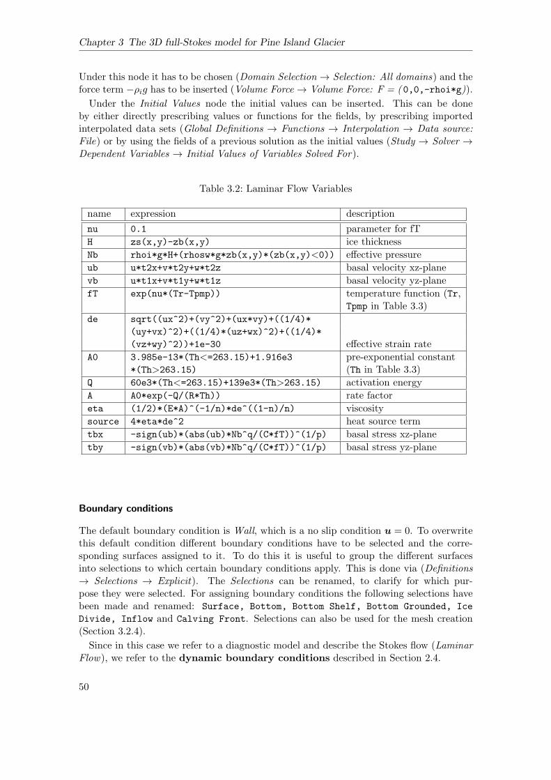
Chapter 3 The 3D full-Stokes model for Pine Island Glacier
Under this node it has to be chosen (Domain Selection → Selection: All domains) and theforce term −ρig has to be inserted (Volume Force → Volume Force: F = ( 0,0,-rhoi*g)).
Under the Initial Values node the initial values can be inserted. This can be doneby either directly prescribing values or functions for the fields, by prescribing importedinterpolated data sets (Global Definitions → Functions → Interpolation → Data source:File) or by using the fields of a previous solution as the initial values (Study → Solver →Dependent Variables → Initial Values of Variables Solved For).
Table 3.2: Laminar Flow Variables
name expression description
nu 0.1 parameter for fT
H zs(x,y)-zb(x,y) ice thickness
Nb rhoi*g*H+(rhosw*g*zb(x,y)*(zb(x,y)<0)) effective pressure
ub u*t2x+v*t2y+w*t2z basal velocity xz-plane
vb u*t1x+v*t1y+w*t1z basal velocity yz-plane
fT exp(nu*(Tr-Tpmp)) temperature function (Tr,Tpmp in Table 3.3)
de sqrt((ux^2)+(vy^2)+(ux*vy)+((1/4)*
(uy+vx)^2)+((1/4)*(uz+wx)^2)+((1/4)*
(vz+wy)^2))+1e-30 effective strain rate
A0 3.985e-13*(Th<=263.15)+1.916e3 pre-exponential constant*(Th>263.15) (Th in Table 3.3)
Q 60e3*(Th<=263.15)+139e3*(Th>263.15) activation energy
A A0*exp(-Q/(R*Th)) rate factor
eta (1/2)*(E*A)^(-1/n)*de^((1-n)/n) viscosity
source 4*eta*de^2 heat source term
tbx -sign(ub)*(abs(ub)*Nb^q/(C*fT))^(1/p) basal stress xz-plane
tby -sign(vb)*(abs(vb)*Nb^q/(C*fT))^(1/p) basal stress yz-plane
Boundary conditions
The default boundary condition is Wall, which is a no slip condition u = 0. To overwritethis default condition different boundary conditions have to be selected and the corre-sponding surfaces assigned to it. To do this it is useful to group the different surfacesinto selections to which certain boundary conditions apply. This is done via (Definitions→ Selections → Explicit). The Selections can be renamed, to clarify for which pur-pose they were selected. For assigning boundary conditions the following selections havebeen made and renamed: Surface, Bottom, Bottom Shelf, Bottom Grounded, Ice
Divide, Inflow and Calving Front. Selections can also be used for the mesh creation(Section 3.2.4).
Since in this case we refer to a diagnostic model and describe the Stokes flow (LaminarFlow), we refer to the dynamic boundary conditions described in Section 2.4.
50

3.2 Implementation
Ice surface
Figure 3.15: Ice surface
The ice surface, highlighted in yellow in Figure 3.15, isseen as a traction free surface (Eq. 2.34) and imple-mented as (Laminar Flow → Open Boundary), whichadds the boundary condition node to the Model BuilderTree. Under the Open Boundary node the surface has tobe selected (Boundary Selection → Selection: Surface).Additionally (Boundary Condition → Boundary Condi-tion: Normal Stress; Normal Stress: f0 = 0) is set.
Ice base
For the diagnostic model and the assumption that basal melt or freeze can be neglected,the kinematic boundary condition is given by Eq. (2.40). For the total ice base,consisting of the floating part, highlighted in blue in Figure 3.16, and the grounded part,highlighted in red in Figure 3.16, this condition is implemented via (Laminar Flow →Weak Constraint). A weak constraint has to be chosen here, as otherwise no smoothvelocity field across the grounding line can be achieved. Weak constraints apply boundaryconditions in an integral sense and are therefore not as strict. They stand in contrast topointwise constraints, which force the nodal value to the constraint and can thus lead tonumerical instability.
Figure 3.16: Ice base
The following settings have to be made: (Bound-ary Selection → Selection: Bottom) and (Weak Con-straint → Constraint type: Bidirectional, symmetric;Constraint expression: -(u*nx+v*ny+w*nz)). Here ithas been made use of the local boundary orthonormalbase vector system that COMSOL provides. It con-sists of the normalised normal vector (n=(nx,ny,nz)) and2 normalised tangential vectors (t1=(t1x,t1y,t1z) andt2=(t2x,t2y,t2z)). The normal vector n always pointsto the exterior of the geometry object. The followingdirections for the tangential vectors are only valid forthe Pine Island Glacier geometry and must be due tothe particular creation process described above (Section
3.2.1). At the base of the geometry object t1 lies in the yz-plane and points in positive ydirection, while t2 lies in the xz-plane and points in positive x direction. This base vectorsystem is also used to implement the basal sliding law described below.
The Constraint expression is evaluated to be zero. The rest of the options is left at thedefault setting.
Ice base - floating
The dynamic boundary condition for the floating ice is given in Eq. (2.37) and im-plemented as (Laminar Flow → Boundary Stress), with the following settings: (BoundarySelection → Selection: Bottom Shelf) and (Boundary Condition → Boundary Condition:Normal stress; Normal stress: f0 = rhow*g*(-z)).
51

Chapter 3 The 3D full-Stokes model for Pine Island Glacier
Ice base - grounded
The boundary condition for the grounded part is given in Eq. (2.42) in form of a slidinglaw. To be implemented it has to be chosen in its inverse form (Eq. (2.43)). In Eq.(2.44a),(2.44b) and (2.44c) the tangential and normal components of the stress vectorσ · n are shown. The stress vector σ · n can thus also be expressed as
σ · n = F−1b ub tx + F−1
b vb ty −Nb n. (3.1)
This is used to implement the boundary condition as (Laminar Flow → Boundary Stress),with the settings: (Boundary Selection → Selection: Bottom Grounded) and (BoundaryCondition → Boundary Condition: General stress; Stress: F =( -Nb*nx+tbx*t2x+tby*t1x,-Nb*ny+tbx*t2y+tby*t1y,-Nb*nz+tbx*t2z+tby*t1z)).
Ice divide
Figure 3.17: Ice divide
The boundary condition for the ice divide, high-lighted in yellow in Figure 3.17, is given in Eq.(2.49) and implemented as (Laminar Flow → Sym-metry). Only the boundary selection (Bound-ary Selection → Selection: Ice Divide) has to bemade.
Calving front
Figure 3.18: Calving front
The boundary condition for the calving front, high-lighted in yellow in Figure 3.18, is given in Eq. (2.52) andimplemented as (Laminar Flow → Boundary Stress),with the following settings: (Boundary Selection → Se-lection: Calving Front) and (Boundary Condition →Boundary Condition: Normal Stress; Normal Stress: f0= rhow*g*(-z)*(z<0)).
52

3.2 Implementation
Inflow
Figure 3.19: Inflow
The boundary condition for the inflow area, highlightedin yellow in Figure 3.19, is given in Eq. (2.53) and im-plemented as (Laminar Flow → Inlet). The followingsettings are made: (Boundary Selection → Selection:Inflow), (Boundary Condition → Boundary Condition:Velocity) and either (Velocity → Normal inflow velocity;U0 = sqrt(uSIA^2+vSIA^2)) or (Velocity → Velocityfield; u0 = ( uSIA,vSIA,0)).
Ice rises
Since the default boundary condition is Wall, it applies to all boundaries that have noother boundary condition assigned to them. The only undefined boundaries are at thispoint the ice rises, that are implemented as holes in the geometric object and thus havesurfaces on the “inside“. The boundary condition for the ice rises is thus given by a noslip condition.
3.2.3 Thermal model
The variables needed for the thermal model, inserted under Local Definitions as mentionedabove, are given in Table 3.3. The thermal model is implemented with the Physics modeHeat Transfer in Fluids. The dependent variable is T . The temperature is solved forwith linear elements (Heat Transfer in Fluids → Discretization → Temperature: Linear).The first subnode is also named Heat Transfer in Fluids (Heat Transfer in Fluids → HeatTransfer in Fluids) and here general entries have to be made (comparable to the FluidProperties node under Laminar Flow). The following settings are made here:
(... → Model Inputs → Absolute pressure: p = Pressure (spf/fp1))(... → Model Inputs → Velocity field: u = Velocity field (spf/fp1))(... → Heat Conduction → Thermal conductivity: k (User defined) = kT (Isotropic))(... → Thermodynamics → Density: ρ (User defined) = rhoi
(... → Thermodynamics → Heat capacity at constant pressure: cp (User defined) = cpT)(... → Thermodynamics → Ratio of specific heats: γ (User defined) = 1 ).
The first two settings, under (... → Model Inputs), create the coupling between the iceflow and the thermal model, such that the calculated velocity and pressure fields serve asinput for the heat advection.Under the Initial Values node the initial values can be inserted as for the ice flow model
in Section 3.2.2.To include the internal heat source term (Eq. (2.13)) a Heat Source node has to be
added (Heat Transfer in Fluids → Heat Source). Under this node the following settingshave to be made: (Domain Selection → Selection: All domains) and (Heat Source →General source: Q (User defined) = source).
53
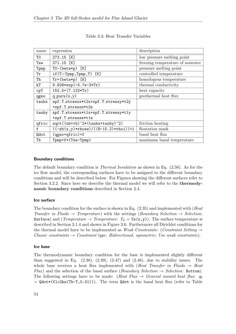
Chapter 3 The 3D full-Stokes model for Pine Island Glacier
Table 3.3: Heat Transfer Variables
name expression description
T0 273.15 [K] low pressure melting point
Tsw 271.15 [K] freezing temperature of seawater
Tpmp T0-(beta*p) [K] pressure melting point
Tr if(T>Tpmp,Tpmp,T) [K] controlled temperature
Th Tr+(beta*p) [K] homologous temperature
kT 9.828*exp(-5.7e-3*Tr) thermal conductivity
cpT 152.5+(7.122*Tr) heat capacity
qgeo q puru(x,y) geothermal heat flux
taubx spf.T stressx*t2x+spf.T stressy*t2y
+spf.T stressz*t2z
tauby spf.T stressx*t1x+spf.T stressy*t1y
+spf.T stressz*t1z
qfric sqrt((ub+vb)^2*(taubx+tauby)^2) friction heating
f ((-zb(x,y)*rhosw)/((H-15.2)*rhoi))>1 floatation mask
Qdot (qgeo+qfric)+f basal heat flux
Tb Tpmp+f*(Tsw-Tpmp) maximum basal temperature
Boundary conditions
The default boundary condition is Thermal Insulation as shown in Eq. (2.50). As for theice flow model, the corresponding surfaces have to be assigned to the different boundaryconditions and will be described below. For Figures showing the different surfaces refer toSection 3.2.2. Since here we describe the thermal model we will refer to the thermody-namic boundary conditions described in Section 2.4.
Ice surface
The boundary condition for the surface is shown in Eq. (2.35) and implemented with (HeatTransfer in Fluids → Temperature) with the settings (Boundary Selection → Selection:Surface) and (Temperature → Temperature: T0 = Ts(x,y)). The surface temperature isdescribed in Section 3.1.4 and shown in Figure 3.6. Furthermore all Dirichlet conditions forthe thermal model have to be implemented as Weak Constraints: (Constraint Setting →Classic constraints → Constraint type: Bidirectional, symmetric; Use weak constraints).
Ice base
The thermodynamic boundary condition for the base is implemented slightly differentthan suggested in Eq. (2.38), (2.39), (2.47) and (2.48), due to stability issues. Thewhole base receives a heat flux implemented with (Heat Transfer in Fluids → HeatFlux ) and the selection of the basal surface (Boundary Selection → Selection: Bottom).The following settings have to be made: (Heat Flux → General inward heat flux: q0= Qdot*(flc2hs(Tb-T,0.01))). The term Qdot is the basal heat flux (refer to Table
54

3.2 Implementation
3.3, a combination of geothermal heat flux, described in Section 3.1.5, and frictionalheat). The function flc2hs is a smoothed Heaviside function with a continuous sec-ond derivative and without overshoot. With the specifying parameters x and scale,flc2hs(x,scale) is a function that approximates the logical expression y = (x > 0)by smoothing the transition within the interval -scale< x< scale. The basal tempera-ture Tb is a spatially variable field that defines the maximal basal temperature that canbe reached and is Tb = Tpmp for grounded areas, and Tb = Tsw for floating areas. Thewhole expression Qdot*(flc2hs(Tb-T,0.01)) thus prescribes a heat flux Qdot, as long asT<(Tb-0.01). When T becomes T≥(Tb-0.01), Qdot is gradually reduced and turns zerowhen T=(Tb+0.01). This procedure ensures a stable way to not let the basal heat fluxincrease the temperature above Tb+0.01. The function is shown in Figure 3.20.
Figure 3.20: Qdot*(flc2hs(Tb-T,0.01))
Inflow
The boundary condition for the inflow is shown in Eq. (2.54) and implemented with aDirichlet condition (Heat Transfer in Fluids → Temperature) with the settings (BoundarySelection → Selection: Inflow), (Temperature → Temperature: T0 = (Tb-Ts(x,y))
/H*(zs(x,y)-z)+Ts(x,y)) and (Constraint Setting → Classic constraints → Constrainttype: Bidirectional, symmetric; Use weak constraints).
Ice divide, calving front and ice rises
The boundary conditions for the remaining boundaries are given by the default conditionThermal Insulation as shown in Eq. (2.50).
3.2.4 Mesh
The mesh of the 3D model for Pine Island Glacier consists of unstructured prism elementsand is shown in Figure 3.21. It is constructed in a number of substeps. This is necessarydue to the very small aspect ratio of Pine Island Glacier, which is the ratio of verticalto horizontal extent ǫ = H L−1. For Pine Island Glacier the vertical extent, which is theaverage thickness, is about 3 km and the horizontal extent about 500 km, which leads to anaspect ratio of the order 10−3. In the main part of the modelling domain in the groundedice, apart from the area adjacent to the grounding line, the biggest gradient of the variables
55
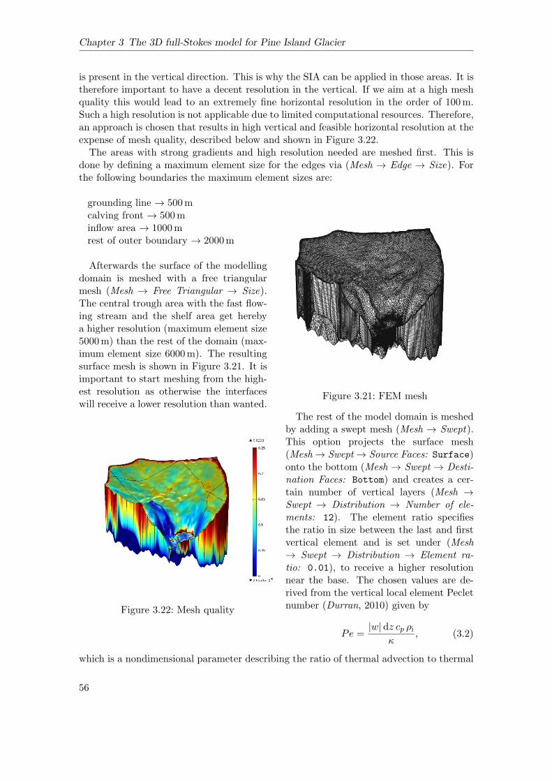
Chapter 3 The 3D full-Stokes model for Pine Island Glacier
is present in the vertical direction. This is why the SIA can be applied in those areas. It istherefore important to have a decent resolution in the vertical. If we aim at a high meshquality this would lead to an extremely fine horizontal resolution in the order of 100m.Such a high resolution is not applicable due to limited computational resources. Therefore,an approach is chosen that results in high vertical and feasible horizontal resolution at theexpense of mesh quality, described below and shown in Figure 3.22.The areas with strong gradients and high resolution needed are meshed first. This is
done by defining a maximum element size for the edges via (Mesh → Edge → Size). Forthe following boundaries the maximum element sizes are:
Figure 3.21: FEM mesh
grounding line → 500mcalving front → 500minflow area → 1000mrest of outer boundary → 2000m
Afterwards the surface of the modellingdomain is meshed with a free triangularmesh (Mesh → Free Triangular → Size).The central trough area with the fast flow-ing stream and the shelf area get herebya higher resolution (maximum element size5000m) than the rest of the domain (max-imum element size 6000m). The resultingsurface mesh is shown in Figure 3.21. It isimportant to start meshing from the high-est resolution as otherwise the interfaceswill receive a lower resolution than wanted.
Figure 3.22: Mesh quality
The rest of the model domain is meshedby adding a swept mesh (Mesh → Swept).This option projects the surface mesh(Mesh → Swept → Source Faces: Surface)onto the bottom (Mesh → Swept → Desti-nation Faces: Bottom) and creates a cer-tain number of vertical layers (Mesh →Swept → Distribution → Number of ele-ments: 12). The element ratio specifiesthe ratio in size between the last and firstvertical element and is set under (Mesh→ Swept → Distribution → Element ra-tio: 0.01), to receive a higher resolutionnear the base. The chosen values are de-rived from the vertical local element Pecletnumber (Durran, 2010) given by
Pe =|w| dz cp ρi
κ, (3.2)
which is a nondimensional parameter describing the ratio of thermal advection to thermal
56

3.2 Implementation
diffusion. At the base of the glacier the stability requirement of Pe < 1 is given almosteverywhere with the above stated values. The final mesh consists of ∼ 370 000 prismelements.
The mesh quality in COMSOL gives a measure of how evenly an element is formed. Theaim is to have elements with the nodes on the surface of a sphere and even length edges.A 2D triangular element would have a mesh quality of 1 for an equilateral triangle and0 if the triangle degenerated into a line. The mesh quality is important so the gradientof the variables solved for does not become too large over the element volume. For meshquality dependent remeshing the default minimum mesh quality is 0.2 and an acceptablemesh quality has to be larger than 0.1 (COMSOL, 2012b). The mesh quality may becomeimportant when using an iterative linear system solver, as it requires a higher mesh qualitythan a direct solver.
3.2.5 Solver
COMSOL Multiphysics© provides a variety of solver choices for solving the FEM modelequations. The solver options can be set under the (Study → Solver Configurations)node of the Model Builder Tree. For computation of a diagnostic solution, a StationarySolver is selected. The settings for the Stationary Solver are adjusted under (...→ SolverConfigurations → Solver → Stationary Solver).
We chose a direct solver, which is uncommon for such a high number of DOF’s, butseems to be the best choice in our case. Iterative solvers work not well due to the badmesh quality described above. The Direct Solver node is added under the Stationary Solvernode in the Model Builder Tree. Here one of three direct solvers, MUMPS, PARDISO orSPOOLES, can be selected.
The chosen Direct Solver can be combined with either a Fully Coupled or Segregatednode. The Fully Coupled node makes the Direct Solver solve for all variables at once. TheSegregated node can be applied such that groups of variables are solved for iteratively. Forthe glacier model this can be done by solving for the temperature T in the Segregated Step1 and for u, v, w and p in the Segregated Step 2. The variables not solved for in a step areheld constant at the previous value of the solution. This way the working memory usagecan be reduced. If sufficient working memory is available, the use of a Fully Coupled nodeis preferable as it converges faster.
Under either, the Fully Coupled or Segregated node, an appropriate setting for Methodand Termination has to be chosen, where the Nonlinear method and the Terminationtechnique are defined. Because the system of model equations is nonlinear, it has to be set(... → Method and Termination → Nonlinear method: Automatic (Newton)/Automatichighly nonlinear (Newton)).
Under the Fully Coupled node the following termination technique is selected: (... →Method and Termination → Termination technique: Iterations or tolerance). This ter-minates the solving process if either a maximum number of iterations is reached (... →Method and Termination → Number of iterations: 25), or the relative error (defined inEq. (3.3)) is smaller than the relative tolerance value chosen, set under (... → Solver→ Stationary Solver → Relative tolerance: 1e-6) and (... → Method and Termination→ Tolerance factor: 1). The Tolerance factor is only meaningful in combination withthe Segregated node, because it can be used to modify the relative tolerance for differentsegregated steps.
57
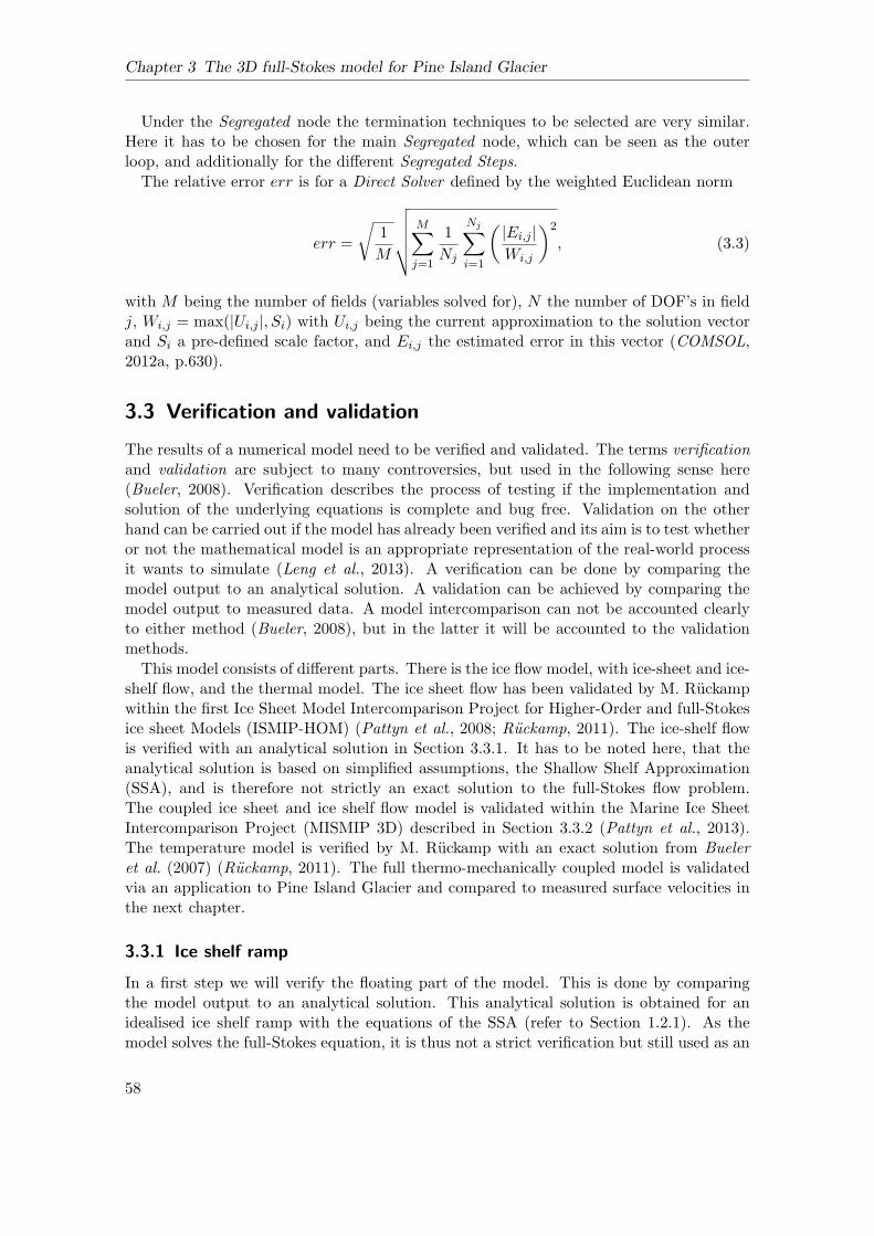
Chapter 3 The 3D full-Stokes model for Pine Island Glacier
Under the Segregated node the termination techniques to be selected are very similar.Here it has to be chosen for the main Segregated node, which can be seen as the outerloop, and additionally for the different Segregated Steps.
The relative error err is for a Direct Solver defined by the weighted Euclidean norm
err =
√
1
M
√
√
√
√
√
M∑
j=1
1
Nj
Nj∑
i=1
(
|Ei,j |
Wi,j
)2
, (3.3)
with M being the number of fields (variables solved for), N the number of DOF’s in fieldj, Wi,j = max(|Ui,j |, Si) with Ui,j being the current approximation to the solution vectorand Si a pre-defined scale factor, and Ei,j the estimated error in this vector (COMSOL,2012a, p.630).
3.3 Verification and validation
The results of a numerical model need to be verified and validated. The terms verificationand validation are subject to many controversies, but used in the following sense here(Bueler, 2008). Verification describes the process of testing if the implementation andsolution of the underlying equations is complete and bug free. Validation on the otherhand can be carried out if the model has already been verified and its aim is to test whetheror not the mathematical model is an appropriate representation of the real-world processit wants to simulate (Leng et al., 2013). A verification can be done by comparing themodel output to an analytical solution. A validation can be achieved by comparing themodel output to measured data. A model intercomparison can not be accounted clearlyto either method (Bueler, 2008), but in the latter it will be accounted to the validationmethods.
This model consists of different parts. There is the ice flow model, with ice-sheet and ice-shelf flow, and the thermal model. The ice sheet flow has been validated by M. Ruckampwithin the first Ice Sheet Model Intercomparison Project for Higher-Order and full-Stokesice sheet Models (ISMIP-HOM) (Pattyn et al., 2008; Ruckamp, 2011). The ice-shelf flowis verified with an analytical solution in Section 3.3.1. It has to be noted here, that theanalytical solution is based on simplified assumptions, the Shallow Shelf Approximation(SSA), and is therefore not strictly an exact solution to the full-Stokes flow problem.The coupled ice sheet and ice shelf flow model is validated within the Marine Ice SheetIntercomparison Project (MISMIP 3D) described in Section 3.3.2 (Pattyn et al., 2013).The temperature model is verified by M. Ruckamp with an exact solution from Bueleret al. (2007) (Ruckamp, 2011). The full thermo-mechanically coupled model is validatedvia an application to Pine Island Glacier and compared to measured surface velocities inthe next chapter.
3.3.1 Ice shelf ramp
In a first step we will verify the floating part of the model. This is done by comparingthe model output to an analytical solution. This analytical solution is obtained for anidealised ice shelf ramp with the equations of the SSA (refer to Section 1.2.1). As themodel solves the full-Stokes equation, it is thus not a strict verification but still used as an
58

3.3 Verification and validation
indication for the right solution. Furthermore the 3D model is compared to the analyticalsolution for 2D flow in the xz-plane. Since the 3D model is axis-symmetric with no lateraldrag, comparison to the 2D flow line solution is valid but does not create any furtherinside to the 3D behaviour (for this refer to Section 3.3.2).
We will show the analytical results for the velocity components u and w and the totalmass balance as − ab, and compare them to the model results. For a detailed derivationof the solutions refer to Greve and Blatter (2009).
We consider an ice shelf that extents from the grounding line at x = 0 to the calvingfront at x = L. The ice thickness H decreases linearly from the thickness at the groundingline Hgl to the thickness at the calving front Hcf, such that
H = Hgl −Hgl −Hcf
Lx. (3.4)
The mean sea level is located at z = 0 and the inflow at the grounding line is given byugl = (ugl, 0, 0). Furthermore steady state conditions and constant rate factor A(T ′) =A = const. are assumed. Table 3.4 gives an overview of the parameter values used in thissection.
Table 3.4: Overview of parameters for the ice shelf ramp
name value description
Hgl 400m ice thickness at grounding lineHcf 200m ice thickness at calving frontL 200 km calving front positionB 10 km extent in y-directionugl 100ma−1 inflow velocity at grounding linen 3 stress exponentA 4.9e-25 s−1 Pa−3 rate factor (for T ′ = −10C)ρi 910 kgm−3 ice densityρsw 1028 kgm−3 sea water densityg 9.81m s−2 acceleration of gravity
In Figure 3.23 the model geometry is shown. The velocity field is indicated by the blackarrows. The red line indicates the sea level and is also the line on which the horizontalvelocity component u is evaluated. The blue line lies at x = L/2 and y = B/2 and is theline where the vertical velocity component w is evaluated.
Since the model consists of an idealised ice shelf, it is not necessary to apply WeakConstraints to the ice base as shown in Section 3.2.2 (Boundary conditions - Ice base).Instead it is sufficient to apply a Symmetry condition as for the Ice Divide (Section 3.2.2- Boundary conditions - Ice divide).
The model is run for different mesh resolutions as listed in Table 3.5. The first column”Identifier” gives a name the simulation is referred to hereafter. Columns ”horizontal” and“layers“ give information about the horizontal and vertical mesh resolution, respectively.Under ”elements” the total number of prism elements and under ”DOF’s” the degrees offreedom, for the different simulations, are listed. The time needed to find a solution, given
59
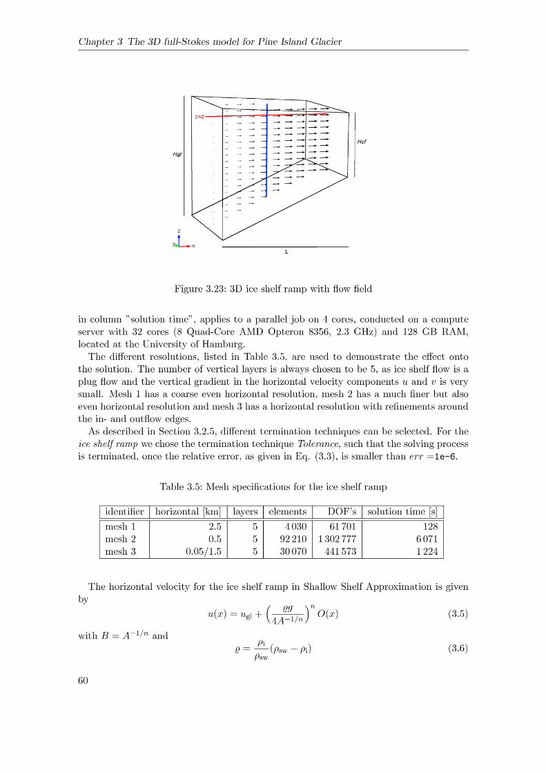
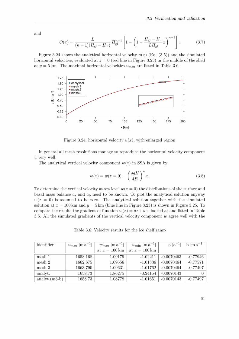
3.3 Verification and validation
and
O(x) =L
(n+ 1)(Hgl −Hcf)Hn+1
gl
[
1−
(
1−Hgl −Hcf
LHglx
)n+1]
. (3.7)
Figure 3.24 shows the analytical horizontal velocity u(x) (Eq. (3.5)) and the simulatedhorizontal velocities, evaluated at z = 0 (red line in Figure 3.23) in the middle of the shelfat y = 5km. The maximal horizontal velocities umax are listed in Table 3.6.
Figure 3.24: horizontal velocity u(x), with enlarged region
In general all mesh resolutions manage to reproduce the horizontal velocity componentu very well.
The analytical vertical velocity component w(z) in SSA is given by
w(z) = w(z = 0)−
(
gH
4B
)n
z. (3.8)
To determine the vertical velocity at sea level w(z = 0) the distributions of the surface andbasal mass balance as and ab need to be known. To plot the analytical solution anywayw(z = 0) is assumed to be zero. The analytical solution together with the simulatedsolution at x = 100 km and y = 5km (blue line in Figure 3.23) is shown in Figure 3.25. Tocompare the results the gradient of function w(z) = az+ b is looked at and listed in Table3.6. All the simulated gradients of the vertical velocity component w agree well with the
Table 3.6: Velocity results for the ice shelf ramp
identifier umax [m a−1] wmax [m a−1] wmin [m a−1] a [a−1] b [m a−1]at x = 100 km at x = 100 km
mesh 1 1658.168 1.09179 -1.02211 -0.0070463 -0.77946mesh 2 1662.675 1.09556 -1.01836 -0.0070464 -0.77571mesh 3 1663.790 1.09631 -1.01762 -0.0070464 -0.77497
analyt. 1658.73 1.86275 -0.24154 -0.0070143 0
analyt.(m3-b) 1658.73 1.08778 -1.01651 -0.0070143 -0.77497
61
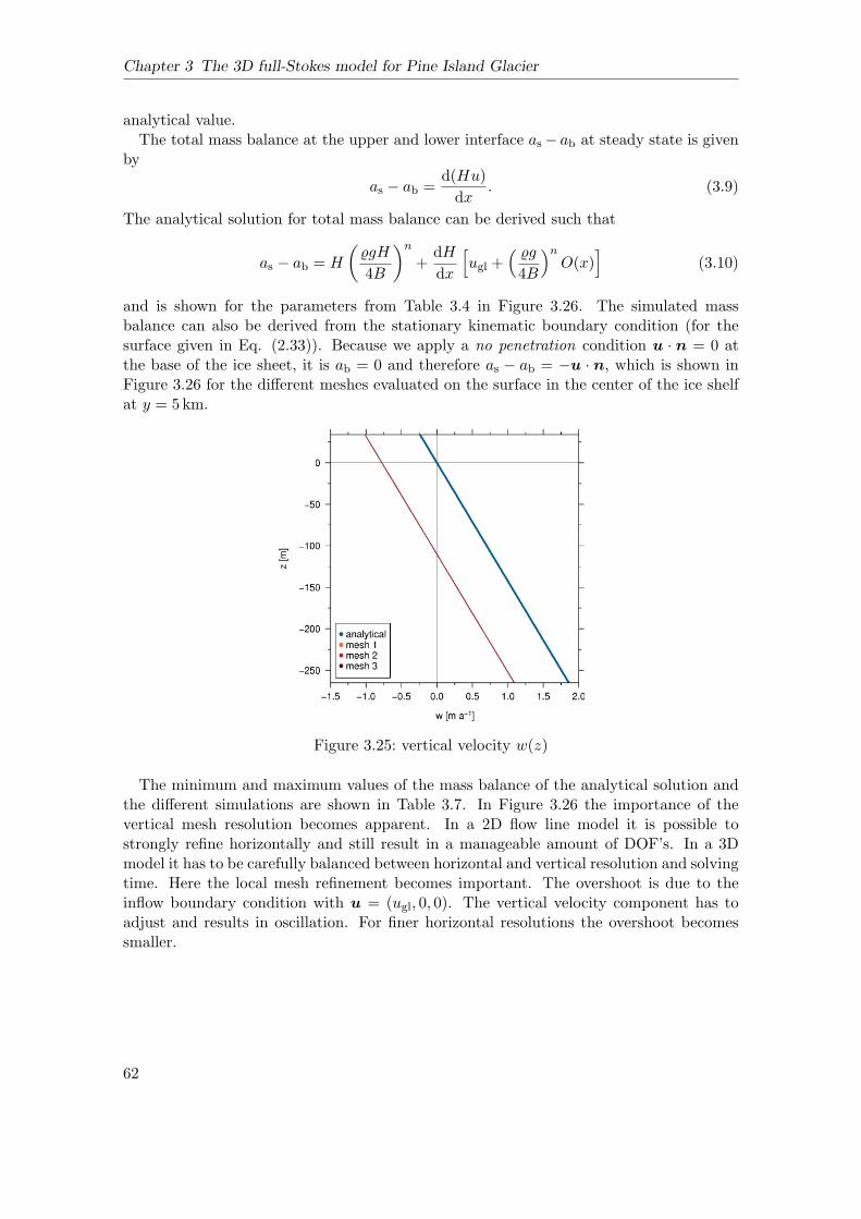
Chapter 3 The 3D full-Stokes model for Pine Island Glacier
analytical value.The total mass balance at the upper and lower interface as− ab at steady state is given
by
as − ab =d(Hu)
dx. (3.9)
The analytical solution for total mass balance can be derived such that
as − ab = H
(
gH
4B
)n
+dH
dx
[
ugl +( g
4B
)nO(x)
]
(3.10)
and is shown for the parameters from Table 3.4 in Figure 3.26. The simulated massbalance can also be derived from the stationary kinematic boundary condition (for thesurface given in Eq. (2.33)). Because we apply a no penetration condition u · n = 0 atthe base of the ice sheet, it is ab = 0 and therefore as − ab = −u · n, which is shown inFigure 3.26 for the different meshes evaluated on the surface in the center of the ice shelfat y = 5km.
Figure 3.25: vertical velocity w(z)
The minimum and maximum values of the mass balance of the analytical solution andthe different simulations are shown in Table 3.7. In Figure 3.26 the importance of thevertical mesh resolution becomes apparent. In a 2D flow line model it is possible tostrongly refine horizontally and still result in a manageable amount of DOF’s. In a 3Dmodel it has to be carefully balanced between horizontal and vertical resolution and solvingtime. Here the local mesh refinement becomes important. The overshoot is due to theinflow boundary condition with u = (ugl, 0, 0). The vertical velocity component has toadjust and results in oscillation. For finer horizontal resolutions the overshoot becomessmaller.
62
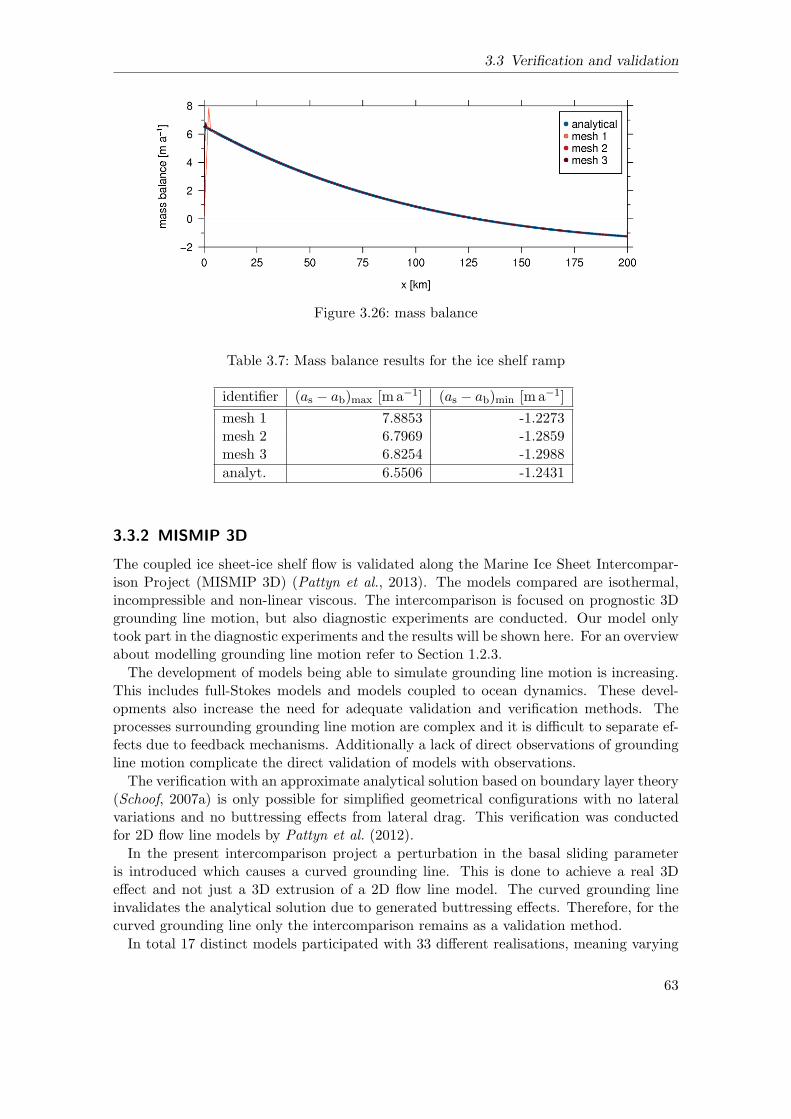
3.3 Verification and validation
Figure 3.26: mass balance
Table 3.7: Mass balance results for the ice shelf ramp
identifier (as − ab)max [m a−1] (as − ab)min [m a−1]
mesh 1 7.8853 -1.2273mesh 2 6.7969 -1.2859mesh 3 6.8254 -1.2988
analyt. 6.5506 -1.2431
3.3.2 MISMIP 3D
The coupled ice sheet-ice shelf flow is validated along the Marine Ice Sheet Intercompar-ison Project (MISMIP 3D) (Pattyn et al., 2013). The models compared are isothermal,incompressible and non-linear viscous. The intercomparison is focused on prognostic 3Dgrounding line motion, but also diagnostic experiments are conducted. Our model onlytook part in the diagnostic experiments and the results will be shown here. For an overviewabout modelling grounding line motion refer to Section 1.2.3.
The development of models being able to simulate grounding line motion is increasing.This includes full-Stokes models and models coupled to ocean dynamics. These devel-opments also increase the need for adequate validation and verification methods. Theprocesses surrounding grounding line motion are complex and it is difficult to separate ef-fects due to feedback mechanisms. Additionally a lack of direct observations of groundingline motion complicate the direct validation of models with observations.
The verification with an approximate analytical solution based on boundary layer theory(Schoof, 2007a) is only possible for simplified geometrical configurations with no lateralvariations and no buttressing effects from lateral drag. This verification was conductedfor 2D flow line models by Pattyn et al. (2012).
In the present intercomparison project a perturbation in the basal sliding parameteris introduced which causes a curved grounding line. This is done to achieve a real 3Deffect and not just a 3D extrusion of a 2D flow line model. The curved grounding lineinvalidates the analytical solution due to generated buttressing effects. Therefore, for thecurved grounding line only the intercomparison remains as a validation method.
In total 17 distinct models participated with 33 different realisations, meaning varying
63
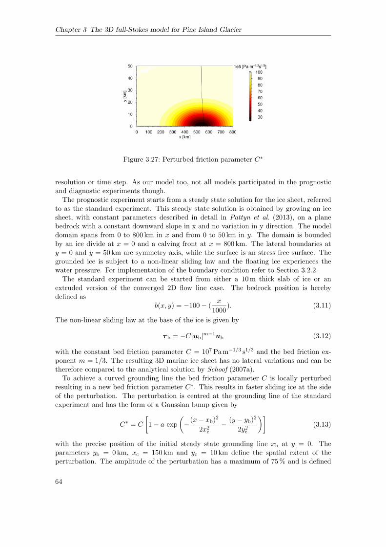
Chapter 3 The 3D full-Stokes model for Pine Island Glacier
Figure 3.27: Perturbed friction parameter C∗
resolution or time step. As our model too, not all models participated in the prognosticand diagnostic experiments though.The prognostic experiment starts from a steady state solution for the ice sheet, referred
to as the standard experiment. This steady state solution is obtained by growing an icesheet, with constant parameters described in detail in Pattyn et al. (2013), on a planebedrock with a constant downward slope in x and no variation in y direction. The modeldomain spans from 0 to 800 km in x and from 0 to 50 km in y. The domain is boundedby an ice divide at x = 0 and a calving front at x = 800 km. The lateral boundaries aty = 0 and y = 50 km are symmetry axis, while the surface is an stress free surface. Thegrounded ice is subject to a non-linear sliding law and the floating ice experiences thewater pressure. For implementation of the boundary condition refer to Section 3.2.2.The standard experiment can be started from either a 10m thick slab of ice or an
extruded version of the converged 2D flow line case. The bedrock position is herebydefined as
b(x, y) = −100− (x
1000). (3.11)
The non-linear sliding law at the base of the ice is given by
τ b = −C|ub|m−1ub (3.12)
with the constant bed friction parameter C = 107 Pam−1/3 s1/3 and the bed friction ex-ponent m = 1/3. The resulting 3D marine ice sheet has no lateral variations and can betherefore compared to the analytical solution by Schoof (2007a).
To achieve a curved grounding line the bed friction parameter C is locally perturbedresulting in a new bed friction parameter C∗. This results in faster sliding ice at the sideof the perturbation. The perturbation is centred at the grounding line of the standardexperiment and has the form of a Gaussian bump given by
C∗ = C
[
1− a exp
(
−(x− xb)
2
2x2c−
(y − yb)2
2y2c
)]
(3.13)
with the precise position of the initial steady state grounding line xb at y = 0. Theparameters yb = 0km, xc = 150 km and yc = 10 km define the spatial extent of theperturbation. The amplitude of the perturbation has a maximum of 75% and is defined
64

3.3 Verification and validation
by the value a = 0.75. The distribution of C∗ can be seen in Figure 3.27, together withthe resulting curved grounding line from the participating full-Stokes model Elmer/Ice(Favier et al., 2012).
Figure 3.28: MISMIP 3D geometry with velocity |u|
The prognostic experiment starts from the steady state solution of the standard ex-periment with the constant C. The perturbed bed friction parameter C∗ is inserted andthe models are run forward for 100 years. This results in a new solution with a curvedgrounding line. The constant C is inserted again and the model is run until it reachesagain a steady state solution. The final steady state should be more or less the same asthe initial standard experiment steady state solution, based on reversibility postulated bySchoof (2007b).
Figure 3.29: us at grounding line Figure 3.30: vs at grounding line
The results of the prognostic experiment are not discussed further here, for detailsrefer to Pattyn et al. (2013). The experimental set up for the prognostic experiment is
65
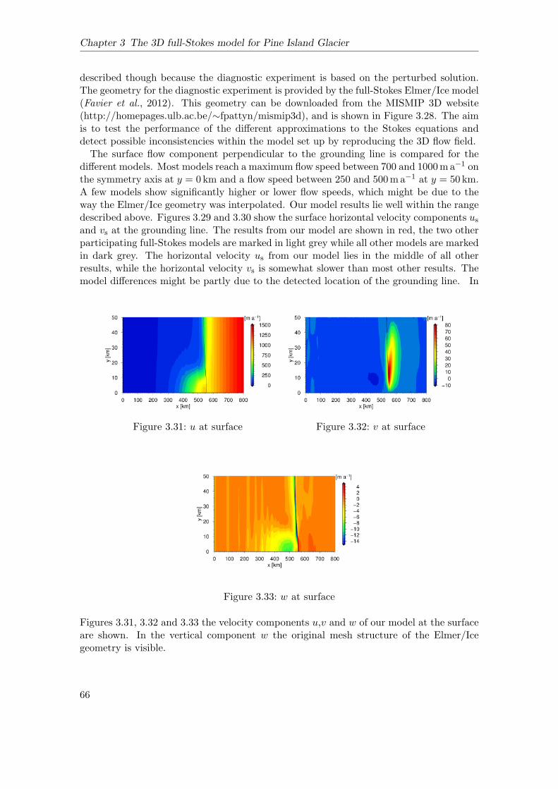
Chapter 3 The 3D full-Stokes model for Pine Island Glacier
described though because the diagnostic experiment is based on the perturbed solution.The geometry for the diagnostic experiment is provided by the full-Stokes Elmer/Ice model(Favier et al., 2012). This geometry can be downloaded from the MISMIP 3D website(http://homepages.ulb.ac.be/∼fpattyn/mismip3d), and is shown in Figure 3.28. The aimis to test the performance of the different approximations to the Stokes equations anddetect possible inconsistencies within the model set up by reproducing the 3D flow field.The surface flow component perpendicular to the grounding line is compared for the
different models. Most models reach a maximum flow speed between 700 and 1000ma−1 onthe symmetry axis at y = 0km and a flow speed between 250 and 500ma−1 at y = 50 km.A few models show significantly higher or lower flow speeds, which might be due to theway the Elmer/Ice geometry was interpolated. Our model results lie well within the rangedescribed above. Figures 3.29 and 3.30 show the surface horizontal velocity components usand vs at the grounding line. The results from our model are shown in red, the two otherparticipating full-Stokes models are marked in light grey while all other models are markedin dark grey. The horizontal velocity us from our model lies in the middle of all otherresults, while the horizontal velocity vs is somewhat slower than most other results. Themodel differences might be partly due to the detected location of the grounding line. In
Figure 3.31: u at surface Figure 3.32: v at surface
Figure 3.33: w at surface
Figures 3.31, 3.32 and 3.33 the velocity components u,v and w of our model at the surfaceare shown. In the vertical component w the original mesh structure of the Elmer/Icegeometry is visible.
66
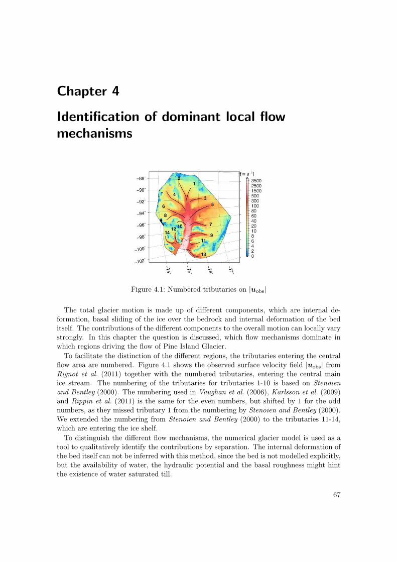
Chapter 4
Identification of dominant local flow
mechanisms
Figure 4.1: Numbered tributaries on |uobs|
The total glacier motion is made up of different components, which are internal de-formation, basal sliding of the ice over the bedrock and internal deformation of the beditself. The contributions of the different components to the overall motion can locally varystrongly. In this chapter the question is discussed, which flow mechanisms dominate inwhich regions driving the flow of Pine Island Glacier.
To facilitate the distinction of the different regions, the tributaries entering the centralflow area are numbered. Figure 4.1 shows the observed surface velocity field |uobs| fromRignot et al. (2011) together with the numbered tributaries, entering the central mainice stream. The numbering of the tributaries for tributaries 1-10 is based on Stenoienand Bentley (2000). The numbering used in Vaughan et al. (2006), Karlsson et al. (2009)and Rippin et al. (2011) is the same for the even numbers, but shifted by 1 for the oddnumbers, as they missed tributary 1 from the numbering by Stenoien and Bentley (2000).We extended the numbering from Stenoien and Bentley (2000) to the tributaries 11-14,which are entering the ice shelf.
To distinguish the different flow mechanisms, the numerical glacier model is used as atool to qualitatively identify the contributions by separation. The internal deformation ofthe bed itself can not be inferred with this method, since the bed is not modelled explicitly,but the availability of water, the hydraulic potential and the basal roughness might hintthe existence of water saturated till.
67
Chapter 4 Identification of dominant local flow mechanisms
In a first step, in Section 4.1, a number of no-slip simulations are conducted, where theice is not allowed to slide over the bed. Even though it is an unrealistic setting for theflow of Pine Island Glacier, where large areas are dominated by strong basal sliding, thesimulations give some insight to the interplay of mechanisms. Along these simulations theeffect of the driving stress is discussed in Section 4.1.1. The basal temperature distributionsolely due to heat conduction is looked at in Section 4.1.2, followed by a discussion aboutthe effect of internal strain heating in Section 4.1.3. The contribution of the internaldeformation to the surface velocity is discussed in Section 4.1.4.
Some findings from the no-slip simulations are subsequently used in Section 4.2 forreference simulations. The technique for these reference simulations, a “quasi-inversion”of a basal sliding parameter, is introduced in Section 4.2.1. The single reference run, whichwill be referred to as a reference for later simulations, is analysed in Section 4.2.2. Thetemperature distribution from the reference run shows a small layer of temperate ice, andis discussed in Section 4.2.3. The effect of considering the water content in the viscosityis discussed in Section 4.2.4, followed by a discussion of the relative contributions of full-Stokes versus SIA terms in Section 4.2.5. Additionally, the reference simulation is used toinvestigate the sensitivity to geothermal heat flux in Section 4.2.6.
Available water at the base of an ice sheet moves along the hydraulic potential. Thehydraulic potential for Pine Island Glacier, which is with a simplified approach solelydependend on geometrical considerations, is looked at in Section 4.3. Additionally thedistribution of the basal roughness is considered in Section 4.46, and used as an indicationfor the presence of sediments below the ice sheet, supported by findings from Smith et al.(2013).
In the last section, Section 4.5, the results are combined for an overall discussion of theflow pattern and the dominant mechanisms in the different tributaries.
All simulations in this and the following chapter are conducted on a high-performancecomputing system at the Alfred-Wegener-Institute, Bremerhaven. The computing systemis composed of one node, consisting of 28 blades with SGI NL5 interconnect, 448 cores (56Intel Xeon E7-8837, 8 cores, 2.66GHz), 3.5 TB RAM (8GB/core) and 140 TB disk space.All following simulations are conducted as parallel jobs on 32 cores.
4.1 No-slip simulations
In Table 4.1 an overview is given of the simulations conducted in this section. Eachsimulation has an identifier in the first column, which will be used in the subsequent textto refer to the according simulation. In column ”qgeo” the data set for the geothermalheat flux is listed, where Purucker stands for the data by Purucker 2012 (updated versionof Fox Maule et al., 2005), Fox for the data from (Fox Maule et al., 2005) and Shapirofor the data from Shapiro and Ritzwoller (2004), all described in Section 3.1.5. Furtherit is listed in column ”source” if the source term for internal heat production (refer toEq. 2.13 and Section 4.1.3) is applied. This is only relevant, if both, the flow modeland the thermal model is solved. In column ”u, p” it is listed if the ice flow modelis used (refer to Section 3.2.2) and in column ”T” if the thermal model is used (referto Section 3.2.3). If the thermal model is not used, either a constant temperature (e.g.T const (-10C)) or a constant temperature field (e.g. T field (qp ref1)), where in brackets,the run from which the temperature field is taken, is listed (refer to Section 4.2). The
68

4.1 No-slip simulations
column ”convergence” contains the minimum error (Eq. (3.3)) reached for the accordingsimulation. All simulations are conducted with a Fully Coupled Solver described in Section3.2.5.
Table 4.1: Overview of simulations conducted for Section ”No-slip simulations”
identifier qgeo source u, p T convergence
qp s Purucker yes yes yes 3.1e-05qp ns Purucker no yes yes 1.2e-03qp T Purucker no no yes 2.7e-10qc up - - yes T const (-10C) 3.9e-07qp up Purucker - yes T field (qp ref1) 5.8e-07qf up Fox - yes T field (qf ref1) 6.7e-07qs up Shapiro - yes T field (qs ref1) 4e-08
4.1.1 Driving stress
When describing glacier flow inertial forces are negligible (refer to Section 2.1.2). Eventhough the ice is in motion, a glacier is effectively in static equilibrium. This gives rise toa force balance analysis, assuming the sum of all forces to be zero (Cuffey and Paterson,2010). The driving stress is balanced by resistive stresses. The driving stress τ d is givenby the gradients of forces exerted by the ice and the resistive stresses are the basal dragτ b, the lateral or wall drag τw and the longitudinal drag τ l, also called internal drag,described by the ice viscosity µ (Benn and Evans, 2010), such that
τ d = τ b + τw + τ l. (4.1)
The driving stress can be interpreted as the action which drives the flow of the ice. Achange in the velocity field can thus be due to a change in either of the components in theabove equation. Thus the flow velocities of a glacier can be influenced by either a changein the driving stress τ d due to surface steepening, shown to happen on Pine Island Glacierby Scott et al. (2009), or by a change in the resistive stresses τ b, τw or τ l (Joughin et al.,2003). The wall drag τw can for example change due to rifts in shear margins (MacGregoret al., 2012), the longitudinal drag τ l due to changes of the ice temperature and the basaldrag τ b for example due to varying availability of sediment or/and water (Smith et al.,2012, 2013).In most cases the basal drag τ b is the most dominant of the resistive stresses (Cuffey and
Paterson, 2010). Following Greve and Blatter (2009) the driving stress can be constructedfor the SIA and is given by
τ d,SIA = −τ b,SIA = −ρigH
∂zs∂x∂zs∂y
, (4.2)
The SIA driving stress τ d,SIA corresponds to the negative of the SIA basal shear stressτ b,SIA. This shows, that the forces are balanced locally at the base of the ice.
69
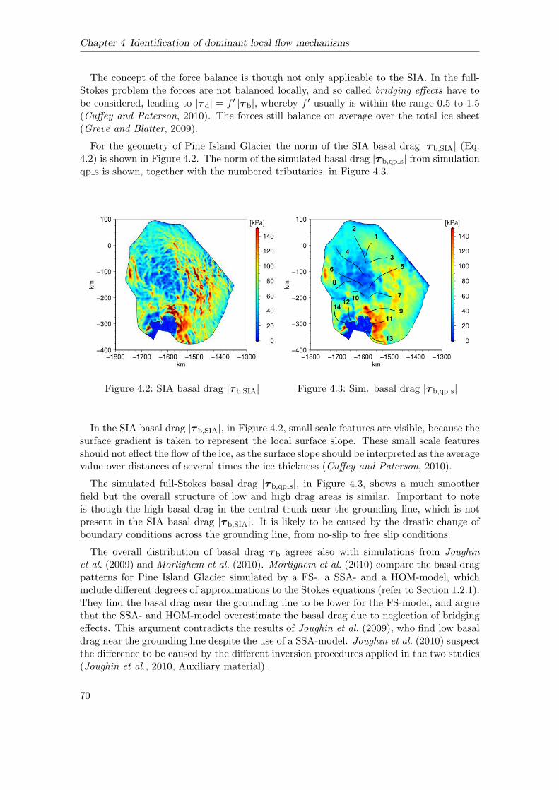
Chapter 4 Identification of dominant local flow mechanisms
The concept of the force balance is though not only applicable to the SIA. In the full-Stokes problem the forces are not balanced locally, and so called bridging effects have tobe considered, leading to |τ d| = f ′ |τ b|, whereby f
′ usually is within the range 0.5 to 1.5(Cuffey and Paterson, 2010). The forces still balance on average over the total ice sheet(Greve and Blatter, 2009).
For the geometry of Pine Island Glacier the norm of the SIA basal drag |τ b,SIA| (Eq.4.2) is shown in Figure 4.2. The norm of the simulated basal drag |τ b,qp s| from simulationqp s is shown, together with the numbered tributaries, in Figure 4.3.
Figure 4.2: SIA basal drag |τ b,SIA| Figure 4.3: Sim. basal drag |τ b,qp s|
In the SIA basal drag |τ b,SIA|, in Figure 4.2, small scale features are visible, because thesurface gradient is taken to represent the local surface slope. These small scale featuresshould not effect the flow of the ice, as the surface slope should be interpreted as the averagevalue over distances of several times the ice thickness (Cuffey and Paterson, 2010).
The simulated full-Stokes basal drag |τ b,qp s|, in Figure 4.3, shows a much smootherfield but the overall structure of low and high drag areas is similar. Important to noteis though the high basal drag in the central trunk near the grounding line, which is notpresent in the SIA basal drag |τ b,SIA|. It is likely to be caused by the drastic change ofboundary conditions across the grounding line, from no-slip to free slip conditions.
The overall distribution of basal drag τ b agrees also with simulations from Joughinet al. (2009) and Morlighem et al. (2010). Morlighem et al. (2010) compare the basal dragpatterns for Pine Island Glacier simulated by a FS-, a SSA- and a HOM-model, whichinclude different degrees of approximations to the Stokes equations (refer to Section 1.2.1).They find the basal drag near the grounding line to be lower for the FS-model, and arguethat the SSA- and HOM-model overestimate the basal drag due to neglection of bridgingeffects. This argument contradicts the results of Joughin et al. (2009), who find low basaldrag near the grounding line despite the use of a SSA-model. Joughin et al. (2010) suspectthe difference to be caused by the different inversion procedures applied in the two studies(Joughin et al., 2010, Auxiliary material).
70

4.1 No-slip simulations
4.1.2 Heat conduction
In this section we are analysing the effect of heat conduction alone, thus not consideringany advection of heat, onto the basal temperature Tb. For this we investigate the resultsfrom simulation qp T (refer to Table 4.1), which is solved for heat conduction alone.The effect of heat conduction can also be estimated with a simplified approach. For
this we need a basal heat flux qgeo, which is described as a temperature gradient normalto a surface. By neglecting the slope of the basal surface under the ice and assuming aconstant thermal conductivity κ, we can write
gradT · n ≈ −∂T
∂z=qgeoκ. (4.3)
Without advection and in equilibrium the gradient can be written such that
∂T
∂z=Ts − Tbzs − zb
=Ts − TbH
= −qgeoκ
⇒ Tb =qgeoH
κ+ Ts. (4.4)
The result of simulation qp T for the homologous basal temperature T ′
b,qp T, the temper-ature relative to the pressure melting point Tpmp, is shown in Figure 4.4. The temperaturesare only shown for the grounded areas, as the shelf is not subject to the geothermal heatflux qgeo.
Figure 4.4: T ′
b,qp T
The simulated basal temperature Tb,qp T reaches temperatures above Tpmp, which is notphysical. For ice the temperature can not be higher than the pressure melting point Tpmp,as it would start to melt. Here we are interested in the effect of the geothermal heat fluxand the ice thickness and therefore ignore for the moment the physically unrealistic setting.With this setting areas can be identified where the ice would be at pressure melting pointTpmp solely due to its thickness and the geothermal heat flux. In Figure 4.4 it can be seen,that with the geothermal heat flux from Purucker and heat conduction alone, almost theentire ice sheet would be at pressure melting point with T ′
b,qp T ≥ 0. Only a small areanear the grounding line is colder, which is due to the relatively thin ice of 10m to 300min that area.
71
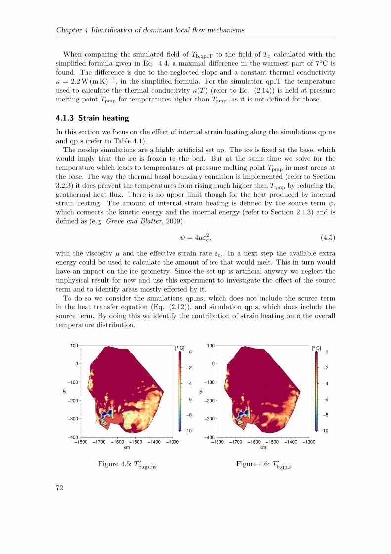
Chapter 4 Identification of dominant local flow mechanisms
When comparing the simulated field of Tb,qp T to the field of Tb calculated with thesimplified formula given in Eq. 4.4, a maximal difference in the warmest part of 7C isfound. The difference is due to the neglected slope and a constant thermal conductivityκ = 2.2W(mK)−1, in the simplified formula. For the simulation qp T the temperatureused to calculate the thermal conductivity κ(T ) (refer to Eq. (2.14)) is held at pressuremelting point Tpmp for temperatures higher than Tpmp, as it is not defined for those.
4.1.3 Strain heating
In this section we focus on the effect of internal strain heating along the simulations qp nsand qp s (refer to Table 4.1).
The no-slip simulations are a highly artificial set up. The ice is fixed at the base, whichwould imply that the ice is frozen to the bed. But at the same time we solve for thetemperature which leads to temperatures at pressure melting point Tpmp in most areas atthe base. The way the thermal basal boundary condition is implemented (refer to Section3.2.3) it does prevent the temperatures from rising much higher than Tpmp by reducing thegeothermal heat flux. There is no upper limit though for the heat produced by internalstrain heating. The amount of internal strain heating is defined by the source term ψ,which connects the kinetic energy and the internal energy (refer to Section 2.1.3) and isdefined as (e.g. Greve and Blatter, 2009)
ψ = 4µε2e, (4.5)
with the viscosity µ and the effective strain rate εe. In a next step the available extraenergy could be used to calculate the amount of ice that would melt. This in turn wouldhave an impact on the ice geometry. Since the set up is artificial anyway we neglect theunphysical result for now and use this experiment to investigate the effect of the sourceterm and to identify areas mostly effected by it.To do so we consider the simulations qp ns, which does not include the source term
in the heat transfer equation (Eq. (2.12)), and simulation qp s, which does include thesource term. By doing this we identify the contribution of strain heating onto the overalltemperature distribution.
Figure 4.5: T ′
b,qp ns Figure 4.6: T ′
b,qp s
72
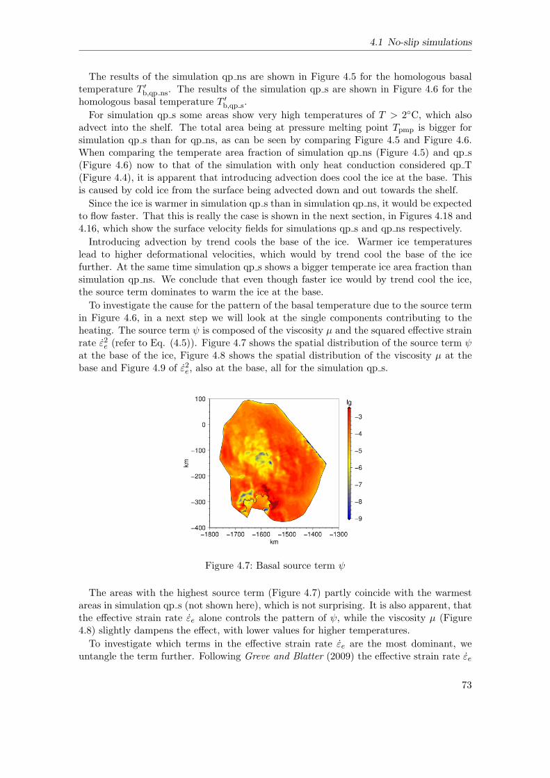
4.1 No-slip simulations
The results of the simulation qp ns are shown in Figure 4.5 for the homologous basaltemperature T ′
b,qp ns. The results of the simulation qp s are shown in Figure 4.6 for thehomologous basal temperature T ′
b,qp s.
For simulation qp s some areas show very high temperatures of T > 2C, which alsoadvect into the shelf. The total area being at pressure melting point Tpmp is bigger forsimulation qp s than for qp ns, as can be seen by comparing Figure 4.5 and Figure 4.6.When comparing the temperate area fraction of simulation qp ns (Figure 4.5) and qp s(Figure 4.6) now to that of the simulation with only heat conduction considered qp T(Figure 4.4), it is apparent that introducing advection does cool the ice at the base. Thisis caused by cold ice from the surface being advected down and out towards the shelf.
Since the ice is warmer in simulation qp s than in simulation qp ns, it would be expectedto flow faster. That this is really the case is shown in the next section, in Figures 4.18 and4.16, which show the surface velocity fields for simulations qp s and qp ns respectively.
Introducing advection by trend cools the base of the ice. Warmer ice temperatureslead to higher deformational velocities, which would by trend cool the base of the icefurther. At the same time simulation qp s shows a bigger temperate ice area fraction thansimulation qp ns. We conclude that even though faster ice would by trend cool the ice,the source term dominates to warm the ice at the base.
To investigate the cause for the pattern of the basal temperature due to the source termin Figure 4.6, in a next step we will look at the single components contributing to theheating. The source term ψ is composed of the viscosity µ and the squared effective strainrate ε2e (refer to Eq. (4.5)). Figure 4.7 shows the spatial distribution of the source term ψat the base of the ice, Figure 4.8 shows the spatial distribution of the viscosity µ at thebase and Figure 4.9 of ε2e, also at the base, all for the simulation qp s.
Figure 4.7: Basal source term ψ
The areas with the highest source term (Figure 4.7) partly coincide with the warmestareas in simulation qp s (not shown here), which is not surprising. It is also apparent, thatthe effective strain rate εe alone controls the pattern of ψ, while the viscosity µ (Figure4.8) slightly dampens the effect, with lower values for higher temperatures.
To investigate which terms in the effective strain rate εe are the most dominant, weuntangle the term further. Following Greve and Blatter (2009) the effective strain rate εe
73

Chapter 4 Identification of dominant local flow mechanisms
Figure 4.8: Basal viscosity µ Figure 4.9: Basal effective strain rate ε2e
is given by
εe =√
ε211 + ε222 + ε11ε22 + ε212 + ε213 + ε223 =
(
∂u
∂x
)2
+
(
∂v
∂y
)2
+∂u
∂x
∂v
∂y
+1
4
(
∂u
∂y+∂v
∂x
)2
+1
4
(
∂u
∂z+∂w
∂x
)2
+1
4
(
∂v
∂z+∂w
∂y
)21/2
.
(4.6)
We now look at the different terms and their contribution to the source term ψ. There-fore we define
D1 =
√
(
∂u∂x
)2; D2 =
√
(
∂v∂y
)2; D3 =
√
(
∂u∂x
∂v∂y
)
D4 =
√
14
(
∂u∂y + ∂v
∂x
)2; D5 =
√
14
(
∂u∂z + ∂w
∂x
)2; D6 =
√
14
(
∂v∂z + ∂w
∂y
)2
The spatial patterns at the base of the ice of the different terms D1-D6 are shownin Figures 4.10-4.15, respectively. Figure 4.10 is displayed in latitude and longitude, tofacilitate the pattern description in terms of cardinal directions, while Figures 4.10-4.15are displayed in Polarstereographic coordinates, as done before.The term D1 (Figure 4.10), which is ∂u
∂x , has the highest values of 10−7.7 to the Southof the ice shelf, near the grounding line, and on the northern side of the curvature of thegrounding line in the central flow area. This displays the effect of the ice flowing from theSouth into the ice shelf, thus in positive x-direction.The term D2 (Figure 4.11) has by far the highest values in the grounded part in flow
direction just before the grounding line. This is not surprising as the term is basically∂v∂y , the main flow direction is in negative y-direction and at the grounding line the basal
condition changes from no-slip to free slip. The values are as high as 10−6.2 in that area.The terms D3 (Figure 4.12) and D4 (Figure 4.13) have similar moderate patterns with
the maximal values of 10−8.1 and 10−8.0, respectively, near the grounding line.
74
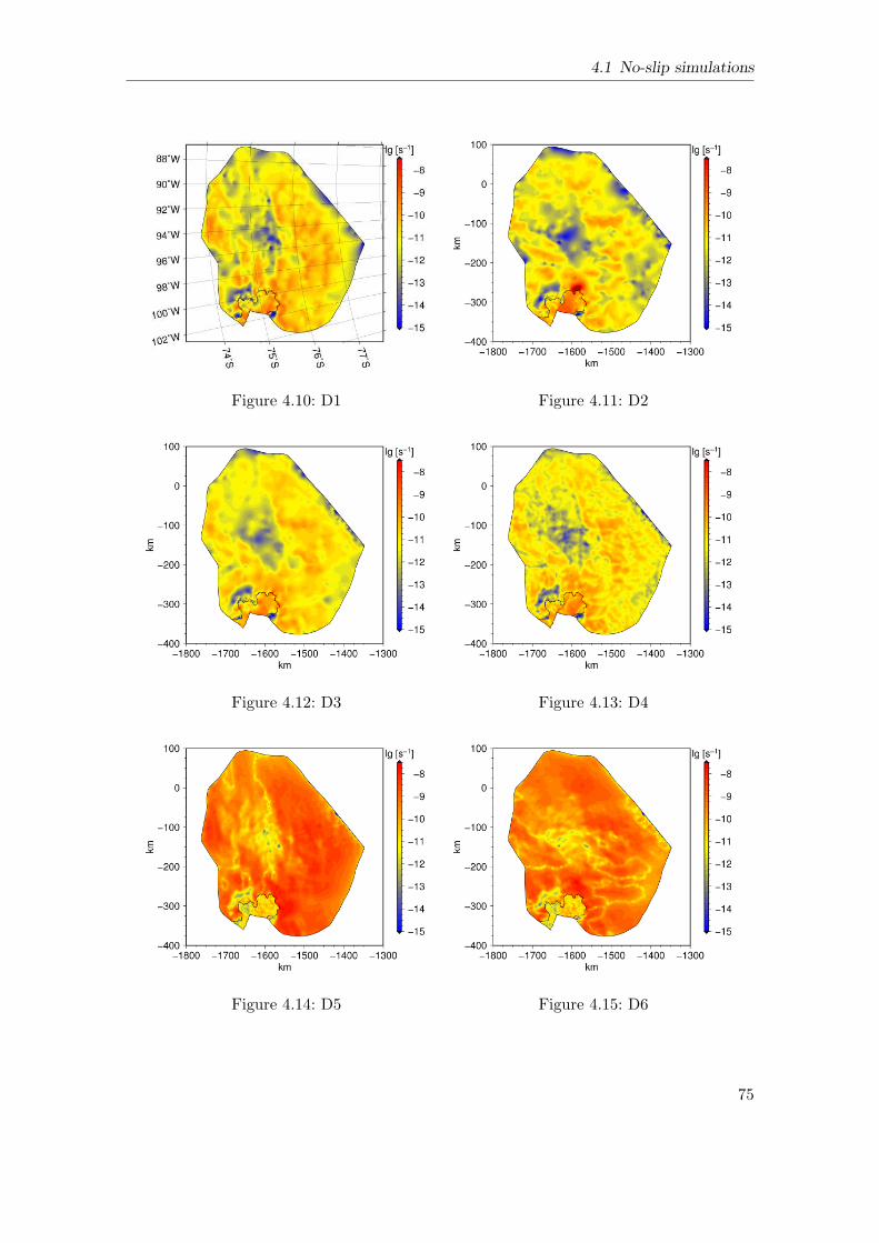
4.1 No-slip simulations
Figure 4.10: D1 Figure 4.11: D2
Figure 4.12: D3 Figure 4.13: D4
Figure 4.14: D5 Figure 4.15: D6
75

Chapter 4 Identification of dominant local flow mechanisms
The terms D5 (Figure 4.14) and D6 (Figure 4.15) have on average much higher valuesthan D1-D4. The maximal value of D5 and D6 is 10−7.1. The term D5 has higher valuesto the South of the ice shelf, again reflecting the flow from the side in positive x-directioninto the ice shelf, while the term D6 has higher values near the grounding line in thecentral flow trough, reflecting the flow in negative y-direction.
All terms reflect the pattern of the driving stress (Figure 4.2-4.3), with the highest shearterms in the areas with largest driving stress.
4.1.4 Internal deformation
Since the ice is fixed at the base, the simulated surface velocity is solely due to internaldeformation. The strain rate ε is strongly influenced by the temperature distributionwithin the ice (refer to Section 2.2.2). By comparing the different simulated surface velocityfields to the measured surface velocity field |uobs|, shown in Figure 4.1 and introduced inSection 3.1.6, we aim to infer some further insight into likely and unlikely temperaturedistributions. A much higher simulated than measured surface velocity could for exampleindicate, that the ice temperature is too high, which leads to softer ice and higher strainrates.
The surface velocity vector fields us, compared in this section, consist of the two hor-izontal velocity components us and vs, such that us = (us, vs). The simulated surfacevelocities from the no-slip simulations are named us,nosl, with nosl being the accordingsimulation identifier from Table 4.1.
The error in measured surface velocity magnitude |uobs| in the Pine Island Glacier regionis 2.5−5.5ma−1 (Rignot et al., 2011, Supporting Online Material). Thus the relative errorfor lower velocities is higher and therefore our method has to be considered with care.
The first simulation considered here is the no-slip simulation qc up, with a constanttemperature of −10C. The temperature −10C is chosen, as it was used in previousstudies to estimate the internal deformation (e.g. Stenoien and Bentley, 2000).
The other three simulations considered here are the no-slip simulations qp up, qf up andqs up. The flow fields are simulated with constant temperature fields, which correspond toa realistic flow field and the heat fluxes from Purucker, Fox and Shapiro (refer to Section3.1.5), respectively.
To receive a realistic temperature field within the ice, the velocity patterns need tobe reproduced. This is achieved with a method introduced in the next section, Section4.2. The procedure described in Section 4.2 is conducted for the different geothermal heatfluxes, with use of results from simulation qp s. These simulations, qp ref1, qf ref1 andqs ref1, show temperature distributions dependent on the flow field and correspondinggeothermal heat fluxes. These temperature fields are used for simulations qp up, qf upand qs up, respectively, as a constant input field.
In the following we show the surface velocity fields |us,nosl|, and the differences betweenthe simulated and measured surface velocity fields |uobs| − |us,nosl|, in the grounded areasfor the four simulations. The surface velocity fields are shown in Figures 4.16, 4.18, 4.20and 4.22 for simulations qc up, qp up, qf up and qs up, respectively. The differencesbetween the simulated and measured surface velocity fields are shown in Figures 4.17,4.19, 4.21 and 4.23 for simulations qc up, qp up, qf up and qs up, respectively.
The differences |uobs|−|us,nosl| are shown from−40 to 65ma−1. Negative values indicatehereby that the simulated surface velocity is too large compared to the measured surface
76
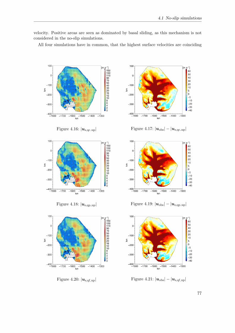
4.1 No-slip simulations
velocity. Positive areas are seen as dominated by basal sliding, as this mechanism is notconsidered in the no-slip simulations.
All four simulations have in common, that the highest surface velocities are coinciding
Figure 4.16: |us,qc up| Figure 4.17: |uobs| − |us,qc up|
Figure 4.18: |us,qp up| Figure 4.19: |uobs| − |us,qp up|
Figure 4.20: |us,qf up| Figure 4.21: |uobs| − |us,qf up|
77
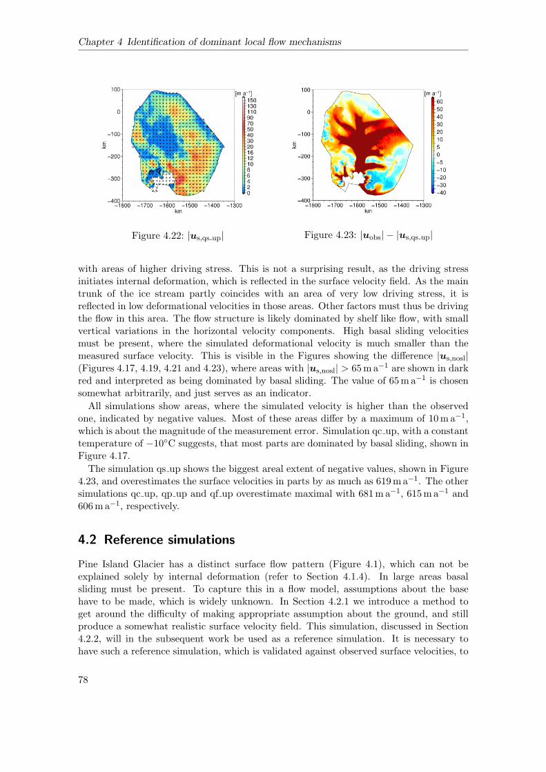
Chapter 4 Identification of dominant local flow mechanisms
Figure 4.22: |us,qs up| Figure 4.23: |uobs| − |us,qs up|
with areas of higher driving stress. This is not a surprising result, as the driving stressinitiates internal deformation, which is reflected in the surface velocity field. As the maintrunk of the ice stream partly coincides with an area of very low driving stress, it isreflected in low deformational velocities in those areas. Other factors must thus be drivingthe flow in this area. The flow structure is likely dominated by shelf like flow, with smallvertical variations in the horizontal velocity components. High basal sliding velocitiesmust be present, where the simulated deformational velocity is much smaller than themeasured surface velocity. This is visible in the Figures showing the difference |us,nosl|(Figures 4.17, 4.19, 4.21 and 4.23), where areas with |us,nosl| > 65ma−1 are shown in darkred and interpreted as being dominated by basal sliding. The value of 65ma−1 is chosensomewhat arbitrarily, and just serves as an indicator.
All simulations show areas, where the simulated velocity is higher than the observedone, indicated by negative values. Most of these areas differ by a maximum of 10ma−1,which is about the magnitude of the measurement error. Simulation qc up, with a constanttemperature of −10C suggests, that most parts are dominated by basal sliding, shown inFigure 4.17.
The simulation qs up shows the biggest areal extent of negative values, shown in Figure4.23, and overestimates the surface velocities in parts by as much as 619ma−1. The othersimulations qc up, qp up and qf up overestimate maximal with 681ma−1, 615ma−1 and606ma−1, respectively.
4.2 Reference simulations
Pine Island Glacier has a distinct surface flow pattern (Figure 4.1), which can not beexplained solely by internal deformation (refer to Section 4.1.4). In large areas basalsliding must be present. To capture this in a flow model, assumptions about the basehave to be made, which is widely unknown. In Section 4.2.1 we introduce a method toget around the difficulty of making appropriate assumption about the ground, and stillproduce a somewhat realistic surface velocity field. This simulation, discussed in Section4.2.2, will in the subsequent work be used as a reference simulation. It is necessary tohave such a reference simulation, which is validated against observed surface velocities, to
78
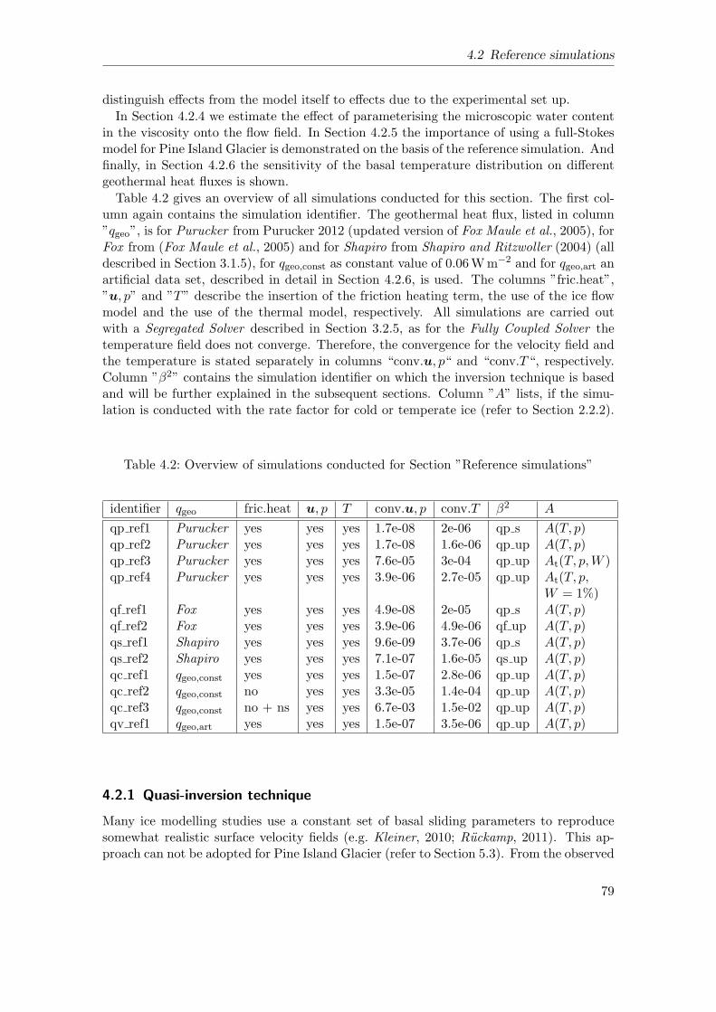
4.2 Reference simulations
distinguish effects from the model itself to effects due to the experimental set up.
In Section 4.2.4 we estimate the effect of parameterising the microscopic water contentin the viscosity onto the flow field. In Section 4.2.5 the importance of using a full-Stokesmodel for Pine Island Glacier is demonstrated on the basis of the reference simulation. Andfinally, in Section 4.2.6 the sensitivity of the basal temperature distribution on differentgeothermal heat fluxes is shown.
Table 4.2 gives an overview of all simulations conducted for this section. The first col-umn again contains the simulation identifier. The geothermal heat flux, listed in column”qgeo”, is for Purucker from Purucker 2012 (updated version of Fox Maule et al., 2005), forFox from (Fox Maule et al., 2005) and for Shapiro from Shapiro and Ritzwoller (2004) (alldescribed in Section 3.1.5), for qgeo,const as constant value of 0.06Wm−2 and for qgeo,art anartificial data set, described in detail in Section 4.2.6, is used. The columns ”fric.heat”,”u, p” and ”T” describe the insertion of the friction heating term, the use of the ice flowmodel and the use of the thermal model, respectively. All simulations are carried outwith a Segregated Solver described in Section 3.2.5, as for the Fully Coupled Solver thetemperature field does not converge. Therefore, the convergence for the velocity field andthe temperature is stated separately in columns “conv.u, p“ and “conv.T“, respectively.Column ”β2” contains the simulation identifier on which the inversion technique is basedand will be further explained in the subsequent sections. Column ”A” lists, if the simu-lation is conducted with the rate factor for cold or temperate ice (refer to Section 2.2.2).
Table 4.2: Overview of simulations conducted for Section ”Reference simulations”
identifier qgeo fric.heat u, p T conv.u, p conv.T β2 A
qp ref1 Purucker yes yes yes 1.7e-08 2e-06 qp s A(T, p)qp ref2 Purucker yes yes yes 1.7e-08 1.6e-06 qp up A(T, p)qp ref3 Purucker yes yes yes 7.6e-05 3e-04 qp up At(T, p,W )qp ref4 Purucker yes yes yes 3.9e-06 2.7e-05 qp up At(T, p,
W = 1%)qf ref1 Fox yes yes yes 4.9e-08 2e-05 qp s A(T, p)qf ref2 Fox yes yes yes 3.9e-06 4.9e-06 qf up A(T, p)qs ref1 Shapiro yes yes yes 9.6e-09 3.7e-06 qp s A(T, p)qs ref2 Shapiro yes yes yes 7.1e-07 1.6e-05 qs up A(T, p)qc ref1 qgeo,const yes yes yes 1.5e-07 2.8e-06 qp up A(T, p)qc ref2 qgeo,const no yes yes 3.3e-05 1.4e-04 qp up A(T, p)qc ref3 qgeo,const no + ns yes yes 6.7e-03 1.5e-02 qp up A(T, p)qv ref1 qgeo,art yes yes yes 1.5e-07 3.5e-06 qp up A(T, p)
4.2.1 Quasi-inversion technique
Many ice modelling studies use a constant set of basal sliding parameters to reproducesomewhat realistic surface velocity fields (e.g. Kleiner, 2010; Ruckamp, 2011). This ap-proach can not be adopted for Pine Island Glacier (refer to Section 5.3). From the observed
79

Chapter 4 Identification of dominant local flow mechanisms
flow pattern of Pine Island Glacier it is apparent, that locally varying basal conditions mustbe present. To capture these, spatial varying assumptions have to be made about basalsliding parameters. A common approach to avoid this problem is to infer the basal slidingparameter from control methods (e.g. MacAyeal, 1992; Joughin et al., 2009; Morlighemet al., 2010). We will briefly introduce this approach, although it is not used here, to thenexplain our simplified method.
The control method approach is prepared by rewriting Eq. (2.43) with
F−1b = C−1
b |τ b|1−pN q
b f(T )−1 = β2, (4.7)
such that
τ b = β2 ub (4.8)
with β2 being the basal sliding parameter to be inferred. It is squared to ensure that thebasal drag represents a sink to the mechanical energy at all points (MacAyeal, 1992).
The explicit problem can be written as
u = G(β) (4.9)
with the velocity field u ∈ U, the sliding parameter β ∈ B and an operator G : B →U representing the model equations. If a set of surface velocity measurements uobs isavailable, an inverse problem formulation can be made to receive a set of β ∈ B, such that
β = G−1(uobs) (4.10)
is fulfilled. For ice sheet modelling there is usually no explicit formulation of G−1. Andthe problem is often either over-determined, such that a solution does not exist, or under-determined, such that the solution is not unique. Therefore a minimisation problem isintroduced, to ensure the model output is as close as possible to the observations
min||G(β)− uobs||. (4.11)
For further details refer to Morlighem (2011).
We chose a different simplified approach. Our aim is to produce a realistic flow fieldto validate the model on a realistic case, and furthermore to initialise the temperaturefield. We call the approach “quasi-inversion” for β2 (cf. Schmeltz et al., 2002). Insteadof minimising the misfit between observed and simulated surface velocities, the followingassumptions are made: the basal drag τ b is very similar if no sliding is allowed and thebasal sliding velocity ub can be approximated by subtracting the surface velocity dueto internal deformation us,nosl from the measured surface velocity field uobs. The basalsliding parameter β2 is then defined as
β2 = |τ b,nosl| (|uobs| − |us,nosl|)−1. (4.12)
The column ”β2” in Table 4.2 indicates from which no-slip simulation the values forEq. (4.12) are taken. Figure 4.24 shows the spatial distribution of β2 for the referencesimulation qp ref2, described in the next section.
80
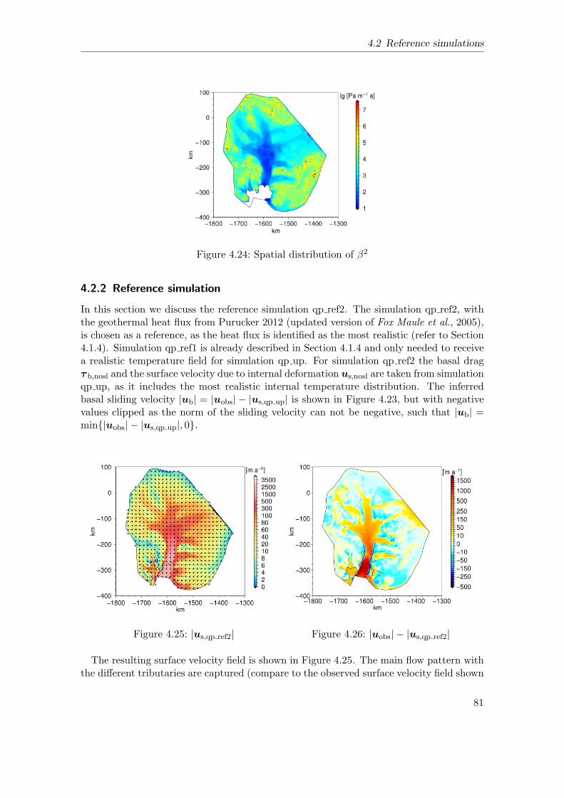
4.2 Reference simulations
Figure 4.24: Spatial distribution of β2
4.2.2 Reference simulation
In this section we discuss the reference simulation qp ref2. The simulation qp ref2, withthe geothermal heat flux from Purucker 2012 (updated version of Fox Maule et al., 2005),is chosen as a reference, as the heat flux is identified as the most realistic (refer to Section4.1.4). Simulation qp ref1 is already described in Section 4.1.4 and only needed to receivea realistic temperature field for simulation qp up. For simulation qp ref2 the basal dragτ b,nosl and the surface velocity due to internal deformation us,nosl are taken from simulationqp up, as it includes the most realistic internal temperature distribution. The inferredbasal sliding velocity |ub| = |uobs| − |us,qp up| is shown in Figure 4.23, but with negativevalues clipped as the norm of the sliding velocity can not be negative, such that |ub| =min|uobs| − |us,qp up|, 0.
Figure 4.25: |us,qp ref2| Figure 4.26: |uobs| − |us,qp ref2|
The resulting surface velocity field is shown in Figure 4.25. The main flow pattern withthe different tributaries are captured (compare to the observed surface velocity field shown
81
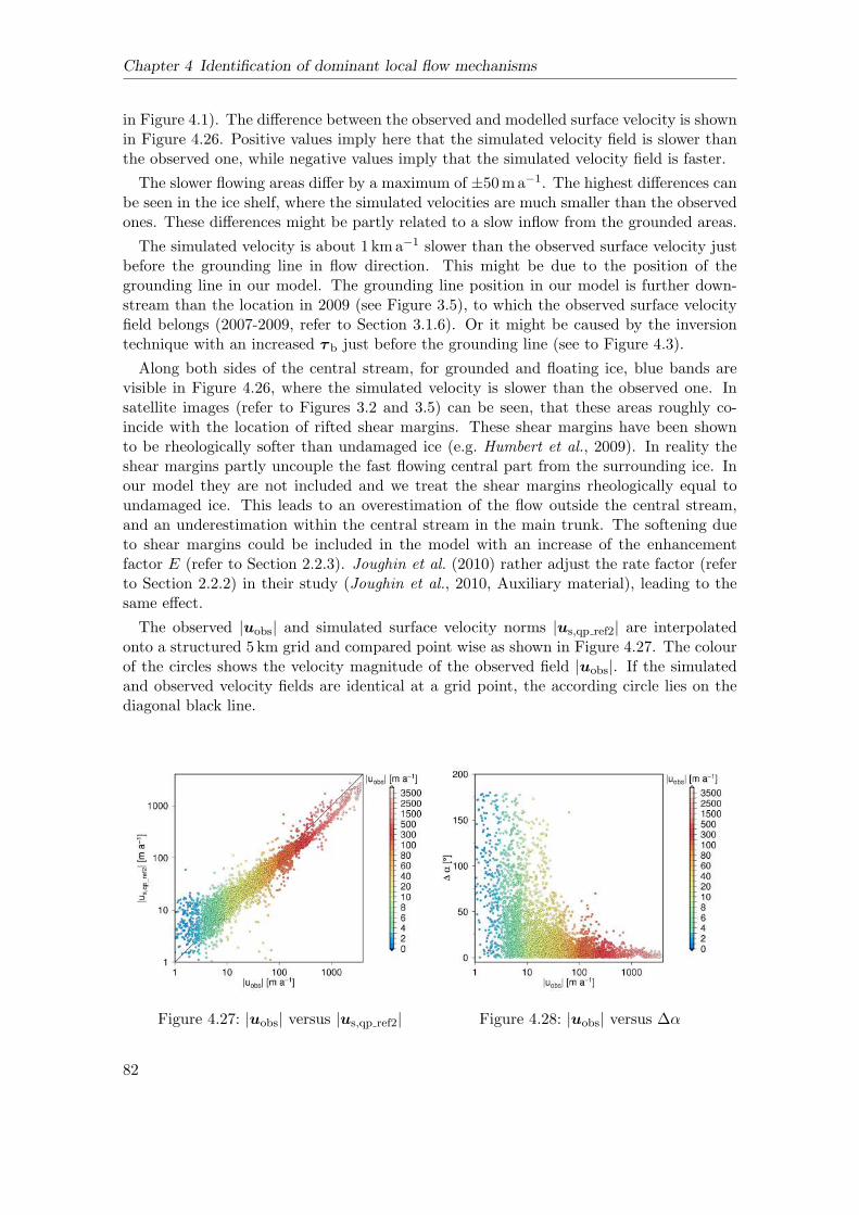
Chapter 4 Identification of dominant local flow mechanisms
in Figure 4.1). The difference between the observed and modelled surface velocity is shownin Figure 4.26. Positive values imply here that the simulated velocity field is slower thanthe observed one, while negative values imply that the simulated velocity field is faster.
The slower flowing areas differ by a maximum of ±50ma−1. The highest differences canbe seen in the ice shelf, where the simulated velocities are much smaller than the observedones. These differences might be partly related to a slow inflow from the grounded areas.
The simulated velocity is about 1 kma−1 slower than the observed surface velocity justbefore the grounding line in flow direction. This might be due to the position of thegrounding line in our model. The grounding line position in our model is further down-stream than the location in 2009 (see Figure 3.5), to which the observed surface velocityfield belongs (2007-2009, refer to Section 3.1.6). Or it might be caused by the inversiontechnique with an increased τ b just before the grounding line (see to Figure 4.3).
Along both sides of the central stream, for grounded and floating ice, blue bands arevisible in Figure 4.26, where the simulated velocity is slower than the observed one. Insatellite images (refer to Figures 3.2 and 3.5) can be seen, that these areas roughly co-incide with the location of rifted shear margins. These shear margins have been shownto be rheologically softer than undamaged ice (e.g. Humbert et al., 2009). In reality theshear margins partly uncouple the fast flowing central part from the surrounding ice. Inour model they are not included and we treat the shear margins rheologically equal toundamaged ice. This leads to an overestimation of the flow outside the central stream,and an underestimation within the central stream in the main trunk. The softening dueto shear margins could be included in the model with an increase of the enhancementfactor E (refer to Section 2.2.3). Joughin et al. (2010) rather adjust the rate factor (referto Section 2.2.2) in their study (Joughin et al., 2010, Auxiliary material), leading to thesame effect.
The observed |uobs| and simulated surface velocity norms |us,qp ref2| are interpolatedonto a structured 5 km grid and compared point wise as shown in Figure 4.27. The colourof the circles shows the velocity magnitude of the observed field |uobs|. If the simulatedand observed velocity fields are identical at a grid point, the according circle lies on thediagonal black line.
Figure 4.27: |uobs| versus |us,qp ref2| Figure 4.28: |uobs| versus ∆α
82
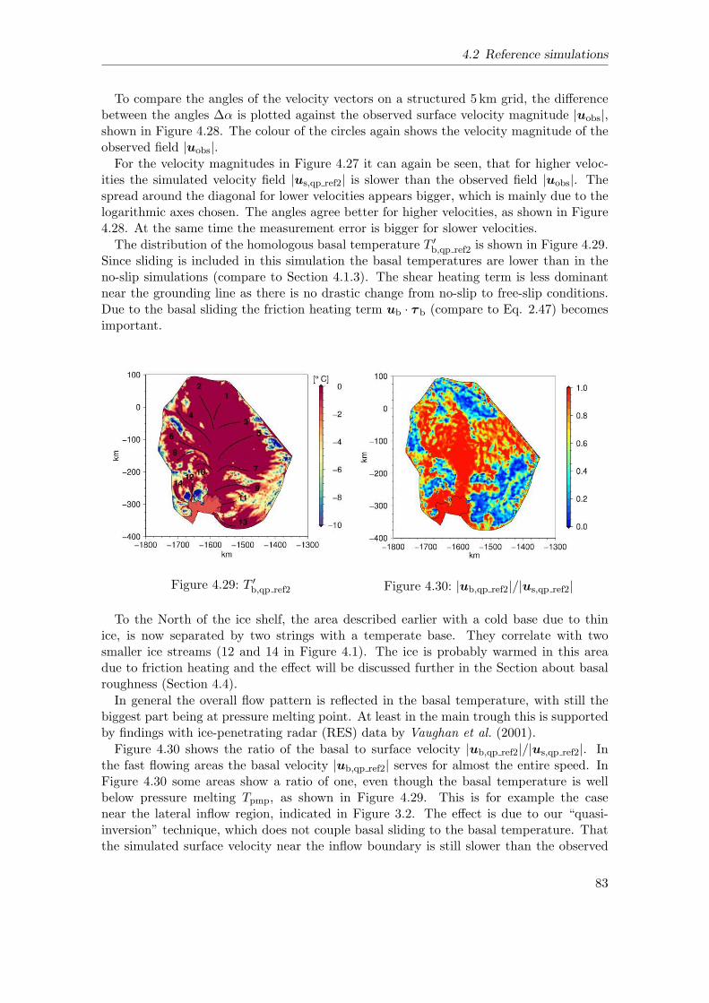
4.2 Reference simulations
To compare the angles of the velocity vectors on a structured 5 km grid, the differencebetween the angles ∆α is plotted against the observed surface velocity magnitude |uobs|,shown in Figure 4.28. The colour of the circles again shows the velocity magnitude of theobserved field |uobs|.
For the velocity magnitudes in Figure 4.27 it can again be seen, that for higher veloc-ities the simulated velocity field |us,qp ref2| is slower than the observed field |uobs|. Thespread around the diagonal for lower velocities appears bigger, which is mainly due to thelogarithmic axes chosen. The angles agree better for higher velocities, as shown in Figure4.28. At the same time the measurement error is bigger for slower velocities.
The distribution of the homologous basal temperature T ′
b,qp ref2 is shown in Figure 4.29.Since sliding is included in this simulation the basal temperatures are lower than in theno-slip simulations (compare to Section 4.1.3). The shear heating term is less dominantnear the grounding line as there is no drastic change from no-slip to free-slip conditions.Due to the basal sliding the friction heating term ub · τ b (compare to Eq. 2.47) becomesimportant.
Figure 4.29: T ′
b,qp ref2 Figure 4.30: |ub,qp ref2|/|us,qp ref2|
To the North of the ice shelf, the area described earlier with a cold base due to thinice, is now separated by two strings with a temperate base. They correlate with twosmaller ice streams (12 and 14 in Figure 4.1). The ice is probably warmed in this areadue to friction heating and the effect will be discussed further in the Section about basalroughness (Section 4.4).
In general the overall flow pattern is reflected in the basal temperature, with still thebiggest part being at pressure melting point. At least in the main trough this is supportedby findings with ice-penetrating radar (RES) data by Vaughan et al. (2001).
Figure 4.30 shows the ratio of the basal to surface velocity |ub,qp ref2|/|us,qp ref2|. Inthe fast flowing areas the basal velocity |ub,qp ref2| serves for almost the entire speed. InFigure 4.30 some areas show a ratio of one, even though the basal temperature is wellbelow pressure melting Tpmp, as shown in Figure 4.29. This is for example the casenear the lateral inflow region, indicated in Figure 3.2. The effect is due to our “quasi-inversion” technique, which does not couple basal sliding to the basal temperature. Thatthe simulated surface velocity near the inflow boundary is still slower than the observed
83
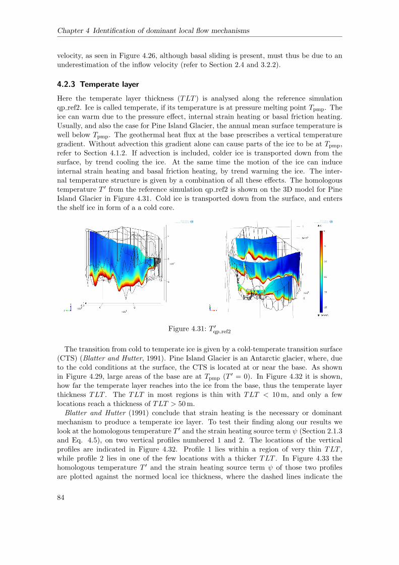
Chapter 4 Identification of dominant local flow mechanisms
velocity, as seen in Figure 4.26, although basal sliding is present, must thus be due to anunderestimation of the inflow velocity (refer to Section 2.4 and 3.2.2).
4.2.3 Temperate layer
Here the temperate layer thickness (TLT ) is analysed along the reference simulationqp ref2. Ice is called temperate, if its temperature is at pressure melting point Tpmp. Theice can warm due to the pressure effect, internal strain heating or basal friction heating.Usually, and also the case for Pine Island Glacier, the annual mean surface temperature iswell below Tpmp. The geothermal heat flux at the base prescribes a vertical temperaturegradient. Without advection this gradient alone can cause parts of the ice to be at Tpmp,refer to Section 4.1.2. If advection is included, colder ice is transported down from thesurface, by trend cooling the ice. At the same time the motion of the ice can induceinternal strain heating and basal friction heating, by trend warming the ice. The inter-nal temperature structure is given by a combination of all these effects. The homologoustemperature T ′ from the reference simulation qp ref2 is shown on the 3D model for PineIsland Glacier in Figure 4.31. Cold ice is transported down from the surface, and entersthe shelf ice in form of a a cold core.
Figure 4.31: T ′
qp ref2
The transition from cold to temperate ice is given by a cold-temperate transition surface(CTS) (Blatter and Hutter, 1991). Pine Island Glacier is an Antarctic glacier, where, dueto the cold conditions at the surface, the CTS is located at or near the base. As shownin Figure 4.29, large areas of the base are at Tpmp (T ′ = 0). In Figure 4.32 it is shown,how far the temperate layer reaches into the ice from the base, thus the temperate layerthickness TLT . The TLT in most regions is thin with TLT < 10m, and only a fewlocations reach a thickness of TLT > 50m.
Blatter and Hutter (1991) conclude that strain heating is the necessary or dominantmechanism to produce a temperate ice layer. To test their finding along our results welook at the homologous temperature T ′ and the strain heating source term ψ (Section 2.1.3and Eq. 4.5), on two vertical profiles numbered 1 and 2. The locations of the verticalprofiles are indicated in Figure 4.32. Profile 1 lies within a region of very thin TLT ,while profile 2 lies in one of the few locations with a thicker TLT . In Figure 4.33 thehomologous temperature T ′ and the strain heating source term ψ of those two profilesare plotted against the normed local ice thickness, where the dashed lines indicate the
84
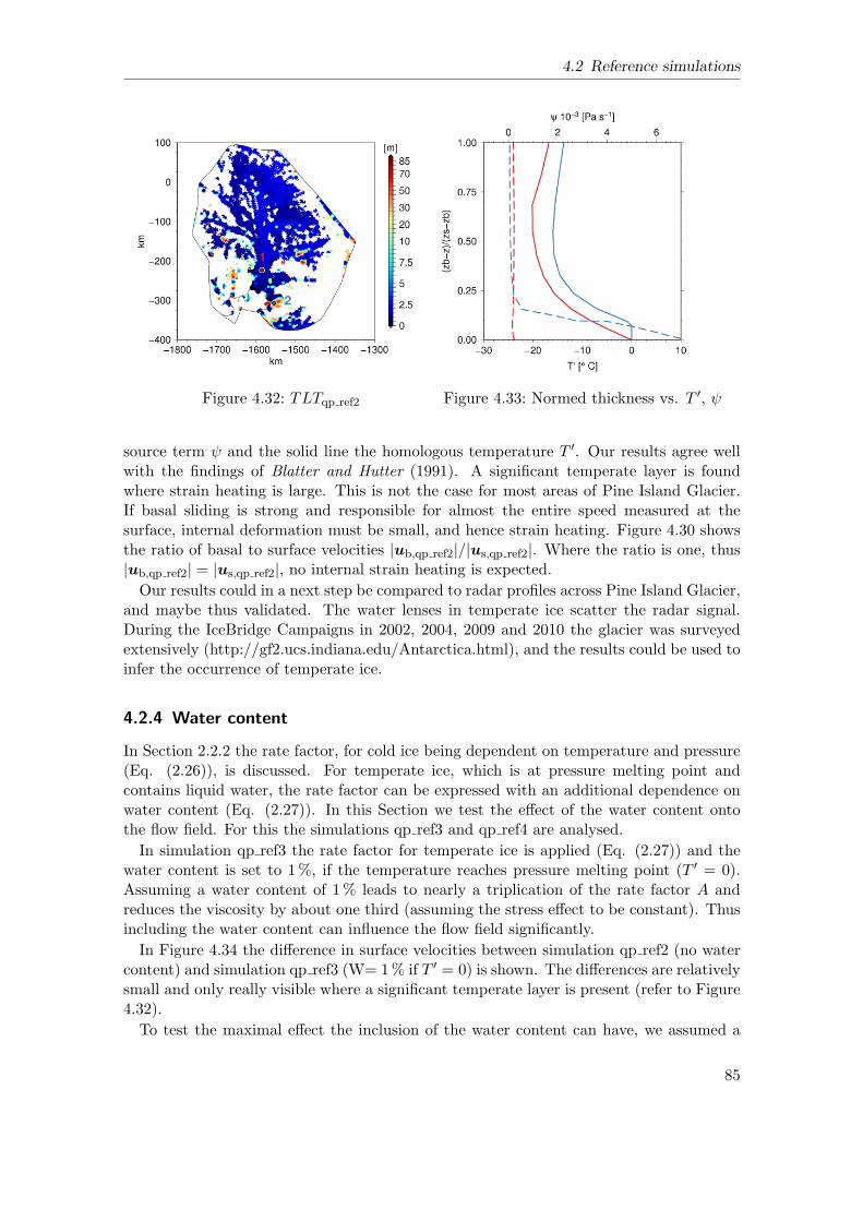
4.2 Reference simulations
Figure 4.32: TLTqp ref2 Figure 4.33: Normed thickness vs. T ′, ψ
source term ψ and the solid line the homologous temperature T ′. Our results agree wellwith the findings of Blatter and Hutter (1991). A significant temperate layer is foundwhere strain heating is large. This is not the case for most areas of Pine Island Glacier.If basal sliding is strong and responsible for almost the entire speed measured at thesurface, internal deformation must be small, and hence strain heating. Figure 4.30 showsthe ratio of basal to surface velocities |ub,qp ref2|/|us,qp ref2|. Where the ratio is one, thus|ub,qp ref2| = |us,qp ref2|, no internal strain heating is expected.
Our results could in a next step be compared to radar profiles across Pine Island Glacier,and maybe thus validated. The water lenses in temperate ice scatter the radar signal.During the IceBridge Campaigns in 2002, 2004, 2009 and 2010 the glacier was surveyedextensively (http://gf2.ucs.indiana.edu/Antarctica.html), and the results could be used toinfer the occurrence of temperate ice.
4.2.4 Water content
In Section 2.2.2 the rate factor, for cold ice being dependent on temperature and pressure(Eq. (2.26)), is discussed. For temperate ice, which is at pressure melting point andcontains liquid water, the rate factor can be expressed with an additional dependence onwater content (Eq. (2.27)). In this Section we test the effect of the water content ontothe flow field. For this the simulations qp ref3 and qp ref4 are analysed.
In simulation qp ref3 the rate factor for temperate ice is applied (Eq. (2.27)) and thewater content is set to 1%, if the temperature reaches pressure melting point (T ′ = 0).Assuming a water content of 1% leads to nearly a triplication of the rate factor A andreduces the viscosity by about one third (assuming the stress effect to be constant). Thusincluding the water content can influence the flow field significantly.
In Figure 4.34 the difference in surface velocities between simulation qp ref2 (no watercontent) and simulation qp ref3 (W= 1% if T ′ = 0) is shown. The differences are relativelysmall and only really visible where a significant temperate layer is present (refer to Figure4.32).
To test the maximal effect the inclusion of the water content can have, we assumed a
85

Chapter 4 Identification of dominant local flow mechanisms
water content of 1% everywhere, not dependent on the temperature, in simulation qp ref4.Practically speaking we nearly tripled the rate factor A everywhere. The result can beseen in Figure 4.35, where we show the difference between the observed surface velocity|uobs| and the simulated one, |us,qp ref4|. It is apparent, that the simulated velocity ismuch higher than the observed one, outside the main central stream. Inside the centralstream the simulated velocity is still too slow. This finding underlines the presumptions,that the difference in speeds must be due to other factors. Surface rifting might be one ofthese.
Figure 4.34: |us,qp ref3| − |us,qp ref2| Figure 4.35: |uobs| − |us,qp ref4|
4.2.5 Full-Stokes vs. SIA
To derive the Shallow Ice Approximation (SIA) (refer to Section 1.2.1 and Greve andBlatter (2009)) one assumption made is that horizontal derivatives of the vertical velocities∂w/∂x and ∂w/∂y are small compared to the vertical derivatives of the horizontal velocities∂u/∂z and ∂v/∂z, and can therefore be neglected. This is shown along a scale analysis (e.g.in Greve and Blatter, 2009), for which typical values for horizontal extents L = 1000 km,vertical extents H = 1km, horizontal velocities U = 100ma−1 and vertical velocitiesW = 0.1ma−1 are introduced and which leads to
U
H= 10−8 s−1 ∼
∂u
∂z∼∂v
∂z, (4.13)
andW
L= 10−14 s−1 ∼
∂w
∂x∼∂w
∂y. (4.14)
To estimate the importance of using a full-Stokes model for the simulation of the flow fieldof Pine Island Glacier, we compare the above shown expected typical values for groundedice to results from simulation qp ref2. The velocity derivatives are shown along verticalprofiles on distinct locations along the central flow line and in two other regions, in andbetween tributaries, indicated in Figure 4.36.
86
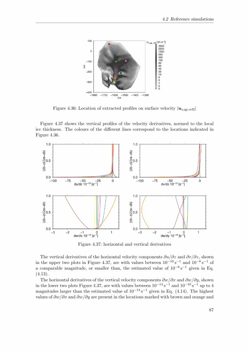
4.2 Reference simulations
Figure 4.36: Location of extracted profiles on surface velocity |us,qp ref2|
Figure 4.37 shows the vertical profiles of the velocity derivatives, normed to the localice thickness. The colours of the different lines correspond to the locations indicated inFigure 4.36.
Figure 4.37: horizontal and vertical derivatives
The vertical derivatives of the horizontal velocity components ∂u/∂z and ∂v/∂z, shownin the upper two plots in Figure 4.37, are with values between 10−10 s−1 and 10−8 s−1 ofa comparable magnitude, or smaller than, the estimated value of 10−8 s−1 given in Eq.(4.13).
The horizontal derivatives of the vertical velocity components ∂w/∂x and ∂w/∂y, shownin the lower two plots Figure 4.37, are with values between 10−14 s−1 and 10−10 s−1 up to 4magnitudes larger than the estimated value of 10−14 s−1 given in Eq. (4.14). The highestvalues of ∂w/∂x and ∂w/∂y are present in the locations marked with brown and orange and
87
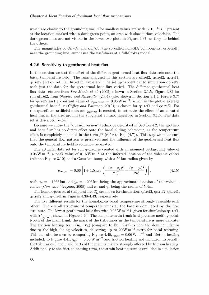
Chapter 4 Identification of dominant local flow mechanisms
which are closest to the grounding line. The smallest values are with ∼ 10−14 s−1 presentat the location marked with a dark green point, an area with slow surface velocities. Thedark green lines are not visible in the lower two plots in Figure 4.37, as they lie behindthe others.
The magnitudes of ∂w/∂x and ∂w/∂y, the so called non-SIA components, especiallynear the grounding line, emphasise the usefulness of a full-Stokes model.
4.2.6 Sensitivity to geothermal heat flux
In this section we test the effect of the different geothermal heat flux data sets onto thebasal temperature field. The runs analysed in this section are qf ref2, qs ref2, qc ref1,qc ref2 and qv ref1, all listed in Table 4.2. The set up is identical to simulation qp ref2,with just the data for the geothermal heat flux varied. The different geothermal heatflux data sets are from Fox Maule et al. (2005) (shown in Section 3.1.5, Figure 3.8) forrun qf ref2, from Shapiro and Ritzwoller (2004) (also shown in Section 3.1.5, Figure 3.7)for qs ref2 and a constant value of qgeo,const = 0.06Wm−2, which is the global averagegeothermal heat flux (Cuffey and Paterson, 2010), is chosen for qc ref1 and qc ref2. Forrun qv ref1 an artificial data set qgeo,art is created, to estimate the effect of an elevatedheat flux in the area around the subglacial volcano described in Section 3.1.5. The dataset is described below.
Because we chose the ”quasi-inversion” technique described in Section 4.2, the geother-mal heat flux has no direct effect onto the basal sliding behaviour, as the temperatureeffect is completely included in the term β2 (refer to Eq. (4.7)). This way we make surethat the general flow pattern is preserved and the influence of the geothermal heat fluxonto the temperature field is somehow separated.
The artificial data set for run qv ref1 is created with an assumed background value of0.06Wm−2, a peak value of 0.15Wm−2 at the inferred location of the volcanic center(refer to Figure 3.10) and a Gaussian bump with a 50 km radius given by
qgeo,art = 0.06
[
1 + 1.5 exp
(
−(x− xv)
2
2x2r−
(y − yv)2
2y2r
)]
, (4.15)
with xv = −1665 km and yv = −205 km being the approximate location of the volcaniccenter (Corr and Vaughan, 2008) and xr and yr being the radius of 50 km.
The homologous basal temperatures T ′
b are shown for simulations qf ref2, qs ref2, qc ref1,qc ref2 and qv ref1 in Figures 4.38-4.43, respectively.
The five different results for the homologous basal temperature strongly resemble eachother. The overall structure of temperate areas at the base is dominated by the flowstructure. The lowest geothermal heat flux with 0.06Wm−2 is given for simulation qc ref1,with T ′
b,qc ref1 shown in Figure 4.40. The complete main trunk is at pressure melting point.North of the main trunk the mark of the tributaries in the temperature is more delicate.The friction heating term (ub · τ b) (compare to Eq. 2.47) is here the dominant factordue to the high sliding velocities, delivering up to 20Wm−2 extra for basal warming.This can also be seen by comparing Figure 4.40, qgeo = 0.06Wm−2 and friction heatingincluded, to Figure 4.41, qgeo = 0.06Wm−2 and friction heating not included. Especiallythe tributaries 3 and 5 and parts of the main trunk are strongly affected by friction heating.Additionally to the friction heating term, the strain heating term is excluded in simulation
88
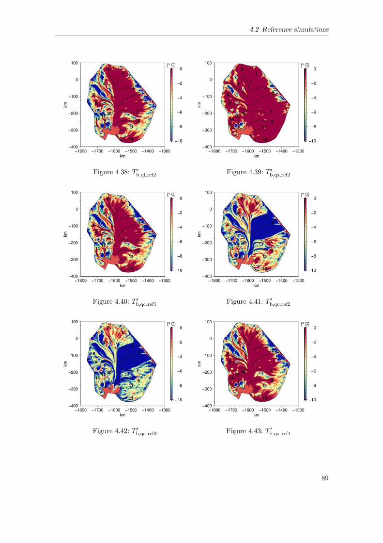
4.2 Reference simulations
Figure 4.38: T ′
b,qf ref2 Figure 4.39: T ′
b,qs ref2
Figure 4.40: T ′
b,qc ref1 Figure 4.41: T ′
b,qc ref2
Figure 4.42: T ′
b,qc ref3 Figure 4.43: T ′
b,qv ref1
89

Chapter 4 Identification of dominant local flow mechanisms
qc ref3. The result T ′
b,qc ref3 is shown in Figure 4.42. It can be seen that tributaries 7, 9,11, 13 are partly warmed by strain heating.
Figure 4.43 shows T ′
b,qv ref1 for the simulation qv ref1, with the artificial high heat fluxaround the volcanic center. Now also areas not affected by strong frictional heat to theNorth of the ice shelf reach pressure melting point Tpmp. This is related to the highergeothermal heat fluxes of qgeo ≥ 0.1Wm−2, as is also the case in simulation qs ref2,shown in Figure 4.39.
4.3 Hydraulic potential
In the previous section we have shown, that large areas at the base of Pine Island Glacierare likely to be at the pressure melting point Tpmp. This finding is supported by a studyfrom Smith et al. (2013). If this potentially available water is likely to accumulate incertain areas, or take distinct routes below the ice sheet, can be investigated by lookingat the hydraulic potential and its gradient. This is done in this section and considered anadditional information about the structure at the glacier bed, supporting or counteractingbasal sliding.
Water at the glacier base does not simply flow downhill following the basal topography,but down the gradient of a hydraulic potential φh, given by Shreve (1972) as
φh = pw + ρwgzb, (4.16)
with pw being the water pressure. Following Cuffey and Paterson (2010) the water pressurepw can be approximated with the assumption that it equals the pressure of the overlyingice and thus
pw = ρig(zs − zb). (4.17)
The hydraulic potential φh equals the basal normal stress Nb for areas that lie below sealevel (refer to Eq. 2.45). The field of the hydraulic potential φh with the approximationsmade thus only depends on the geometry of the ice and is shown in Figure 4.44.
Figure 4.44: Hydraulic potential φh
90

4.4 Basal roughness
The potential gradient, which determines the opposite direction of flow, is given withpw from Eq. (4.17) as
gradφh = grad pw + ρwg grad zb = ρig grad zs + (ρw − ρi)g grad zb. (4.18)
The contribution of the ice surface gradient grad zs to the potential gradient gradφh, andthus to the water flow path, is ∼ 10 times higher than the contribution of the gradient ofthe basal topography grad zb (Cuffey and Paterson, 2010).
The field of the potential gradient norm |gradφh| together with the normalised vectorfield −gradφh, indicating the direction of flow, is shown in Figure 4.45.
Figure 4.45: Potential gradient −gradφh
The water flows from high to low potential and thus mainly into the basal trough inwhich the central fast flowing trunk of the glacier is located, as shown in Figure 4.44. Thelowest potential is situated all along the grounding line. The strength and direction ofthe water path can be seen in Figure 4.45, where the potential gradient is shown. Sometributaries show a higher tendency to accumulate water than others, with actual flowpatterns depending also on water availability, and will be further discussed in Section 4.5.
4.4 Basal roughness
The basal roughness measure itself simply classifies the roughness of the bed. For anintroduction to basal properties below ice sheets refer to Section 1.1.3. For a more detaileddescription of the derivation process of basal roughness, explicitly of the single and two-parameter roughness index, refer to Section 5.5.1. Rippin et al. (2011) assess the singleparameter basal roughness index beneath Pine Island Glacier from a RES data set. Thebasal roughness distribution in the Pine Island area is shown in Figure 4.46. The roughnessmeasure ξ is shown with a logarithmic scale, such that the most negative values represent
91

Chapter 4 Identification of dominant local flow mechanisms
the smoothest bed. Rippin et al. (2011) interpret the smoother areas as marine sedimentbasins beneath Pine Island Glacier, deposited after disappearance of the West AntarcticIce Sheet in the Pliocene (5.3 − 2.6Ma ago) or Pleistocene (2.6 − 0.01Ma ago) (Walkerand Geissman, 2009). For an overview of the geologic history and the marine ice sheetinstability refer to Section 1.1.1 and 1.1.2, respectively.
By combining the basal roughness distribution with information about potential wateravailability and the bed strength, indicated by the basal shear stress discussed in Section4.1.1, we aim at further distinguishing the basal properties below Pine Island Glacier.
4.5 Discussion
Figure 4.1 shows the observed surface velocity field |uobs| from Rignot et al. (2011) togetherwith the numbered tributaries, entering the central main flow field. The basal topography,for a detailed description refer to Section 3.1.1, is shown in Figure 4.47, together with thenumbered tributaries.
Figure 4.46: Single parameter roughness ξ Figure 4.47: Bed topography zb
In Table 4.3 a classification of the relative importance of different factors influencingthe flow field for the single tributaries is listed. For this a variety of fields are considered.In the first column the tributary number is listed. In column “basal topography” is listed,if the location of the tributary coincides with a depression in the basal topography, thusis directed by it. In column ”τd ” is listed, if a high driving stress coincides with thepath of the tributary. Column ”Tpmp” lists, if the base below the tributary is at pressuremelting point. For this all geothermal heat flux data sets are considered. To estimate theimportance of the friction heating to the temperate base, another run is conducted wherethe friction heating term is not included. In column ”friction heating dominant for Tpmp”is listed, if the friction heating term is crucial for the ice base to be at pressure meltingpoint Tpmp. Column ”hydraulic sink” lists if the tributary coincides with a hydraulic sink.And in column ”roughness” is listed, if the tributary is underlain by a smooth bed, andthus maybe sediment.
To distinguish the relative strength of the signal, a V stands for a strong signal, a v foran intermediate signal, a x for a signal that is not present and a X for an exclusion of the
92

4.5 Discussion
signal.
Table 4.3: Strength of signal. V: strong signal, v: intermediate signal , x: no clear signal,X: clearly no signal.
tributary basal τd Tpmp friction heating hydraulic low ξtopography dominant for Tpmp sink
1 v v V x v x2 v x V x v v3 v v V V v x4 v X v v x V5 x v V V V x6 v X V x x V7 V x V v V V8 x X v v v v9 v V V V v X10 x v v v v v11 X V V x V X12 v v v x V V13 v v v v v X14 v v v x V x
Tributary 1 is a small tributary entering the main ice stream from the South-East.It has a small signal in the basal topography. The driving stress seems to initiate thetributary, which flows at a intermediate speed of 50−100ma−1. The basal temperature isin all simulations at pressure melting point, independent of friction heating. The hydraulicgradient suggests a water flow in ice flow direction with an intermediate strength. Thebase below the tributary is relatively rough. We thus suggest tributary 1 to be initiated bythe driving stress, and sustained due the trough in the basal topography, which channelsthe basal melt water, as the base is at pressure melting.
Tributary 2 can also be seen as the most distant end of the main stream from thegrounding line. The tributary enters the main stream from the North-East at similarspeed as tributary 1. It also shows a small signal in the basal topography. The basaltemperature is also, independent of friction heating, at pressure melting point. In contrastto tributary 1, the driving stress at tributary 2 is very small. Instead the basal roughnessis low below the tributary. It is no major hydraulic sink, but a small signal is noticeable,also following the ice flow direction. The tributary seems to be driven by the low basalroughness, suggesting a long existence of the tributary, and a temperate base, while thedirection is guided by a basal trough.
Tributary 3 enters the main ice stream from the South. It shows a small signal in thebasal topography and the driving stress. The base is temperate, although mainly due tofriction heating. The base below the tributary is relatively rough and a small signal in thehydraulic gradient is visible. We suggest that the tributary sustains itself by lubricationof the base due to friction heating.
A seismic survey by Smith et al. (2013) across tributary 4 and the main stream, where
93

Chapter 4 Identification of dominant local flow mechanisms
tributaries 1 to 3 have already entered, suggests a geological boundary towards the South,separating sedimentary strata from basement rocks. They suggest, that the geologicalboundary coincides with a change from a thick sediment layer to a much thinner sedimentlayer, towards tributary 3. This thinner layer could be increasingly eroded, possibly leadingto a change in basal drag and subsequently a change in flow speed.
Tributary 4 is characterised by a very low driving stress and low basal roughness. Itenters the main stream from the North-East and has a small signal in the basal topography.The basal temperature below the tributary is partly at pressure melting point, and evenless so if friction heating is not considered. The hydraulic gradient has no clear signalbelow tributary 4. Smith et al. (2013) find evidence for a relatively thick sedimentarybasin below tributary 4, coinciding with the low roughness. We suggest tributary 4 to bemainly driven by the basal sediments, which can not sustain the basal drag.
Tributary 5 enters the main stream from the South-East. The flow direction crosses adeep trough in the basal topography, not directly being guided by it. The flow is initiatedby the driving stress, while the base is temperate, mainly caused by friction heating.Below the tributary a hydraulic sink is present. The base is at the onset of the tributaryrelatively rough, becoming smoother were it meets the main stream.
Tributary 6 enters from North-East. The driving stress is very low, and so is the basalroughness. An intermediate signal in the basal topography is present below the glacier.The central part of tributary 6 is at Tpmp, not strongly dependent on friction heating. Thehydraulic gradient has no strong signal.
Tributary 7 enters the main stream from the South and is clearly steered by the basaltopography. It is characterised by a small driving stress and a low basal roughness. Thewater, if available, would flow right below the tributary, with a strong signal in the hy-draulic gradient. The base is temperate, in the onset region not due to friction heating.
Tributary 8 flows into tributary 6 from the North-West. It is not topographically steeredand the driving stress is very small. The base is only partly at Tpmp, and friction heatingis partly responsible for the heating. The water below the tributary would possibly accu-mulate in a topographic low, but not necessarily follow the flow path of the ice. The baseis characterised by low roughness.
Tributary 9 enters the main stream from the South, relatively close to the groundingline. The signal in the basal topography is small, but present. The driving stress is high,especially near the grounding line, coinciding with a rough base. The base is temperate,mainly due to friction heating. The base below the tributary is no clear hydraulic sink,but the water flow direction agrees with the ice flow direction. We suggest the main factorfor the flow of this tributary to be the driving stress, whose existence is supported by arough base.
Tributary 10 flows with velocities around 20− 40ma−1 relatively slow from the Northinto the main stream. It has no signal in the basal topography. In the onset the drivingstress is high, but reduces rapidly in flow direction. The basal temperature is largely atTpmp, partly depending on friction heating. The base becomes smoother towards the mainstream. The hydraulic gradient supports the flow direction.
Tributary 11 flows from the South into the ice shelf. It is not steered by the basaltopography, but instead by a high driving stress. The base below the tributary is relativelyrough. It has a temperate base, independent of friction heating. And the hydraulicgradient is strong, with the water flowing towards the grounding line.
Tributary 13 is the furthest west and enters the Amundsen sea from the South-West. It
94
4.5 Discussion
does not directly flow into the ice shelf of Pine Island Glacier. A small signal in the basaltopography is present, combined with a relatively high driving stress, slightly to the Eastof the tributary. The base is temperate, largely due to friction heating. The hydraulicgradient strongly supports the flow direction and the base is rough, becoming smoothertowards the ice shelf.Tributaries 12 and 14 enter the ice shelf from the East and North-East, respectively.
The have both a small signal in the basal topography. The driving stress for both is higherin the onset region, reducing towards the grounding line. They have a temperate base,which is not necessarily due to friction heating. Both tributaries are strong hydraulic sinks,steering the water in ice flow direction towards the grounding line. The main differencebetween the two tributaries is the basal roughness. While tributary 12 has a relativelysmooth bed, tributary 14 flows over a rougher base.Additionally to the above classification of different mechanisms being important for the
flow pattern of the single tributaries, we have shown, in Section 4.1.4, that the geothermalheat flux from Shapiro and Ritzwoller (2004) leads in our simulations to ice temperatureswhich in turn lead to velocities higher than the measured surface velocities. We thereforeinfer that the geothermal heat flux from Shapiro and Ritzwoller (2004) is unrealisticallyhigh in the Pine Island area. For further simulations we thus use the geothermal heat fluxfrom Purucker 2012 (updated version of Fox Maule et al., 2005), as it gives similar resultsto, and is an updated version from Fox Maule et al. (2005).We also show, that the “quasi-inversion” technique, introduced in Section 4.2.1, leads to
good results in reproducing the flow field for Pine Island Glacier, shown in Section 4.2.2.We analyse the basal temperate layer in Section 4.2.3. The mismatch between simulatedand observed surface velocities is not due to the use of the rate factor A for cold ice, whichis shown in Section 4.2.4. The importance of using a full-Stokes model for our simulationsis shown in Section 4.2.5.
95

Chapter 5
Basal sliding
In this chapter we are analysing the impact of different sliding and slip assumptions ontothe modelled flow field of Pine Island Glacier. In the previous chapter we avoided thechallenge to find an appropriate formulation for basal sliding, by introducing the “quasi-inversion” technique described in Section 4.2.1. In this chapter we address basal slidingand its difficulties and implications, which are already briefly introduced in Section 1.2.2.To do so we will first give an overview of existing theories dealing with basal sliding inSection 5.1, and thereafter test their applicability for Pine Island Glacier with the ice flowmodel, in Section 5.3.
In the last two Sections we will use some measured, and therefore afore known, infor-mation about the bed, which is the basal roughness, already briefly introduced in Section1.1.3 and 4.4, and include this in different ways into the sliding law. In Section 5.4 wecombine the spatial structure of the basal roughness to the sliding law. And finally, inSection 5.5, we test the applicability of an existing theory by Li et al. (2010), which alsoconnects the measured basal roughness to basal sliding, for Pine Island Glacier.
5.1 Theory - Basal sliding
In the theories about basal motion generally two different mechanisms are considered,which are for one sliding over a hard bed, described in Section 5.1.1, and secondly, slidingover or with a deformable bed, described in Section 5.1.2. These mechanisms are arbitrarilycomplex, but need to be broken down into their main components, to formulate a relationthat can be applied as a boundary condition for the modelling of ice dynamics.
To establish a basal sliding relation for an individual glacier, usually an empirical ap-proach is taken and the relations are calibrated for the specific glacier (Cuffey and Pater-son, 2010). This was done for Pine Island Glacier in a variety of studies (e.g. Joughin et al.,2009, 2010; Morlighem et al., 2010), and also here in Section 4.2. Still we aim at findingsome physical framework to base the sliding relation on and not having to arbitrarily choseparameters.
Rapid sliding over hard beds only occurs if basal temperatures are at pressure meltingpoint Tpmp, while the underlying till or sediment layer only deforms rapidly if it is saturatedwith water at pressure close to the weight of the overlying ice (Cuffey and Paterson, 2010).
In the following we will give a short introduction to the original ideas, on which thecommonly applied sliding relations are based, as they are of importance in the subsequentsections of this chapter.
97
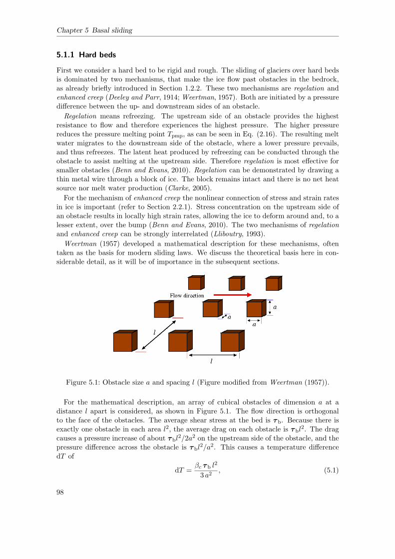
Chapter 5 Basal sliding
5.1.1 Hard beds
First we consider a hard bed to be rigid and rough. The sliding of glaciers over hard bedsis dominated by two mechanisms, that make the ice flow past obstacles in the bedrock,as already briefly introduced in Section 1.2.2. These two mechanisms are regelation andenhanced creep (Deeley and Parr, 1914; Weertman, 1957). Both are initiated by a pressuredifference between the up- and downstream sides of an obstacle.
Regelation means refreezing. The upstream side of an obstacle provides the highestresistance to flow and therefore experiences the highest pressure. The higher pressurereduces the pressure melting point Tpmp, as can be seen in Eq. (2.16). The resulting meltwater migrates to the downstream side of the obstacle, where a lower pressure prevails,and thus refreezes. The latent heat produced by refreezing can be conducted through theobstacle to assist melting at the upstream side. Therefore regelation is most effective forsmaller obstacles (Benn and Evans, 2010). Regelation can be demonstrated by drawing athin metal wire through a block of ice. The block remains intact and there is no net heatsource nor melt water production (Clarke, 2005).
For the mechanism of enhanced creep the nonlinear connection of stress and strain ratesin ice is important (refer to Section 2.2.1). Stress concentration on the upstream side ofan obstacle results in locally high strain rates, allowing the ice to deform around and, to alesser extent, over the bump (Benn and Evans, 2010). The two mechanisms of regelationand enhanced creep can be strongly interrelated (Lliboutry, 1993).
Weertman (1957) developed a mathematical description for these mechanisms, oftentaken as the basis for modern sliding laws. We discuss the theoretical basis here in con-siderable detail, as it will be of importance in the subsequent sections.
Figure 5.1: Obstacle size a and spacing l (Figure modified from Weertman (1957)).
For the mathematical description, an array of cubical obstacles of dimension a at adistance l apart is considered, as shown in Figure 5.1. The flow direction is orthogonalto the face of the obstacles. The average shear stress at the bed is τ b. Because there isexactly one obstacle in each area l2, the average drag on each obstacle is τ bl
2. The dragcauses a pressure increase of about τ bl
2/2a2 on the upstream side of the obstacle, and thepressure difference across the obstacle is τ bl
2/a2. This causes a temperature differencedT of
dT =βc τ b l
2
3 a2, (5.1)
98
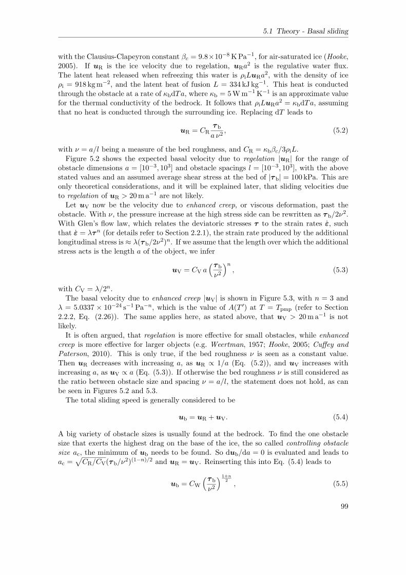
5.1 Theory - Basal sliding
with the Clausius-Clapeyron constant βc = 9.8×10⁻⁸KPa−1, for air-saturated ice (Hooke,2005). If uR is the ice velocity due to regelation, uRa
2 is the regulative water flux.The latent heat released when refreezing this water is ρiLuRa
2, with the density of iceρi = 918 kgm−2, and the latent heat of fusion L = 334 kJ kg−1. This heat is conductedthrough the obstacle at a rate of κbdTa, where κb = 5Wm−1K−1 is an approximate valuefor the thermal conductivity of the bedrock. It follows that ρiLuRa
2 = κbdTa, assumingthat no heat is conducted through the surrounding ice. Replacing dT leads to
uR = CRτ b
a ν2, (5.2)
with ν = a/l being a measure of the bed roughness, and CR = κbβc/3ρiL.Figure 5.2 shows the expected basal velocity due to regelation |uR| for the range of
obstacle dimensions a = [10−3, 103] and obstacle spacings l = [10−3, 103], with the abovestated values and an assumed average shear stress at the bed of |τ b| = 100 kPa. This areonly theoretical considerations, and it will be explained later, that sliding velocities dueto regelation of uR > 20ma−1 are not likely.
Let uV now be the velocity due to enhanced creep, or viscous deformation, past theobstacle. With ν, the pressure increase at the high stress side can be rewritten as τ b/2ν
2.With Glen’s flow law, which relates the deviatoric stresses τ to the strain rates ε, suchthat ε = λτn (for details refer to Section 2.2.1), the strain rate produced by the additionallongitudinal stress is ≈ λ(τ b/2ν
2)n. If we assume that the length over which the additionalstress acts is the length a of the object, we infer
uV = CV a(τ b
ν2
)n, (5.3)
with CV = λ/2n.The basal velocity due to enhanced creep |uV| is shown in Figure 5.3, with n = 3 and
λ = 5.0337 × 10⁻²⁴ s−1 Pa−n, which is the value of A(T ′) at T = Tpmp (refer to Section2.2.2, Eq. (2.26)). The same applies here, as stated above, that uV > 20ma−1 is notlikely.It is often argued, that regelation is more effective for small obstacles, while enhanced
creep is more effective for larger objects (e.g. Weertman, 1957; Hooke, 2005; Cuffey andPaterson, 2010). This is only true, if the bed roughness ν is seen as a constant value.Then uR decreases with increasing a, as uR ∝ 1/a (Eq. (5.2)), and uV increases withincreasing a, as uV ∝ a (Eq. (5.3)). If otherwise the bed roughness ν is still considered asthe ratio between obstacle size and spacing ν = a/l, the statement does not hold, as canbe seen in Figures 5.2 and 5.3.The total sliding speed is generally considered to be
ub = uR + uV. (5.4)
A big variety of obstacle sizes is usually found at the bedrock. To find the one obstaclesize that exerts the highest drag on the base of the ice, the so called controlling obstaclesize ac, the minimum of ub needs to be found. So dub/da = 0 is evaluated and leads toac =
√
CR/CV(τ b/ν2)(1−n)/2 and uR = uV. Reinserting this into Eq. (5.4) leads to
ub = CW
(τ b
ν2
)1+n2, (5.5)
99
Chapter 5 Basal sliding
Figure 5.2: |uR| due to regelation Figure 5.3: |uV| due to enhanced creep
with CW = 2CV
√
CR/CV. This is valid for beds where all objects have the controllingobstacle size ac (estimated to be ac ≈ 0.5m (Clarke, 2005); ac ≈ 0.01 − 0.1m (Cuffeyand Paterson, 2010)), or for beds with a homogeneous distribution of roughness elements- so-called white roughness.
With n = 3 the sliding velocity ub then varies with τ 2b, as shown in Eq. (5.5). When
following the above made statement, where the bed roughness ν is seen as a constantvalue, for absence of small obstacles < ac, a smooth bedrock possibly caused by abrasion,sliding occurs mainly by enhanced creep, and thus varies with τ 3
b, as seen in Eq. (5.3).On the other hand, if only obstacles < ac are present, sliding is dominated by regelationand thus varies linearly with τ b, as shown in Eq. (5.2). In all cases sliding velocity alsosensitively depends on the basal roughness ν.
The bed structure assumed by Weertman (1957) is highly artificial. Nye (1969) andKamb (1970) also analysed basal sliding by considering a more realistic bed structure con-sisting of superimposed sine waves. The mechanisms that let the ice flow past obstaclesare also regelation and enhanced flow. For an exact solution of their approach they un-fortunately had to assume a linear rheology (n = 1) for the ice. For a nonlinear rheology,Kamb (1970) still obtained an approximate solution. Without going into detail of theirtheory, it can be noted that Nye (1969) and Kamb (1970) both conclude that ub ∝ τ b/ν
2
for the linear rheology, which is also the case for the theory by Weertman (1957, Eq. (5.5with n = 1). Kamb’s nonlinear theory leads to ub ∝ τ 2
b, at least for some roughnessspectra (Hooke, 2005).
Measurements show an upper limit for basal velocities due to hard bed sliding (Cuffeyand Paterson, 2010). This is not reflected in Figures 5.2 and 5.3, which show very highsliding velocities for some combinations of obstacle size and spacing. Faster basal slidingcan for example occur due to underlying weak deformable substrate, discussed in the nextsection. Hard bed sliding velocities > 20ma−1 are only possible if water filled cavitiesare considered (e.g. Lliboutry, 1968). Water filled cavities on the downstream side of anobstacle can form, when the water pressure pw exceeds the compressive normal stress(Cuffey and Paterson, 2010). The dominant quantity is thus the effective pressure, orbasal normal stress, Nb (refer to Eq. (2.45)). Cavities reduce the contact between the ice
100
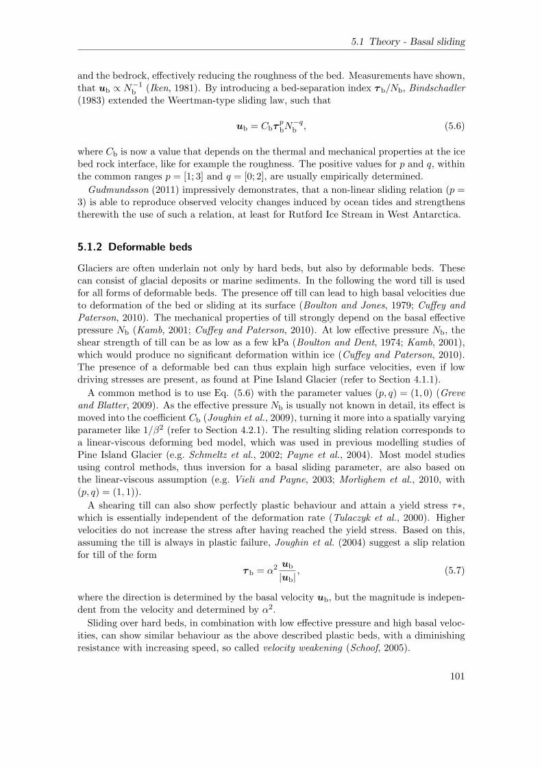
5.1 Theory - Basal sliding
and the bedrock, effectively reducing the roughness of the bed. Measurements have shown,that ub ∝ N−1
b (Iken, 1981). By introducing a bed-separation index τ b/Nb, Bindschadler(1983) extended the Weertman-type sliding law, such that
ub = CbτpbN
−qb , (5.6)
where Cb is now a value that depends on the thermal and mechanical properties at the icebed rock interface, like for example the roughness. The positive values for p and q, withinthe common ranges p = [1; 3] and q = [0; 2], are usually empirically determined.
Gudmundsson (2011) impressively demonstrates, that a non-linear sliding relation (p =3) is able to reproduce observed velocity changes induced by ocean tides and strengthenstherewith the use of such a relation, at least for Rutford Ice Stream in West Antarctica.
5.1.2 Deformable beds
Glaciers are often underlain not only by hard beds, but also by deformable beds. Thesecan consist of glacial deposits or marine sediments. In the following the word till is usedfor all forms of deformable beds. The presence off till can lead to high basal velocities dueto deformation of the bed or sliding at its surface (Boulton and Jones, 1979; Cuffey andPaterson, 2010). The mechanical properties of till strongly depend on the basal effectivepressure Nb (Kamb, 2001; Cuffey and Paterson, 2010). At low effective pressure Nb, theshear strength of till can be as low as a few kPa (Boulton and Dent, 1974; Kamb, 2001),which would produce no significant deformation within ice (Cuffey and Paterson, 2010).The presence of a deformable bed can thus explain high surface velocities, even if lowdriving stresses are present, as found at Pine Island Glacier (refer to Section 4.1.1).
A common method is to use Eq. (5.6) with the parameter values (p, q) = (1, 0) (Greveand Blatter, 2009). As the effective pressure Nb is usually not known in detail, its effect ismoved into the coefficient Cb (Joughin et al., 2009), turning it more into a spatially varyingparameter like 1/β2 (refer to Section 4.2.1). The resulting sliding relation corresponds toa linear-viscous deforming bed model, which was used in previous modelling studies ofPine Island Glacier (e.g. Schmeltz et al., 2002; Payne et al., 2004). Most model studiesusing control methods, thus inversion for a basal sliding parameter, are also based onthe linear-viscous assumption (e.g. Vieli and Payne, 2003; Morlighem et al., 2010, with(p, q) = (1, 1)).
A shearing till can also show perfectly plastic behaviour and attain a yield stress τ∗,which is essentially independent of the deformation rate (Tulaczyk et al., 2000). Highervelocities do not increase the stress after having reached the yield stress. Based on this,assuming the till is always in plastic failure, Joughin et al. (2004) suggest a slip relationfor till of the form
τ b = α2 ub
|ub|, (5.7)
where the direction is determined by the basal velocity ub, but the magnitude is indepen-dent from the velocity and determined by α2.
Sliding over hard beds, in combination with low effective pressure and high basal veloc-ities, can show similar behaviour as the above described plastic beds, with a diminishingresistance with increasing speed, so called velocity weakening (Schoof, 2005).
101
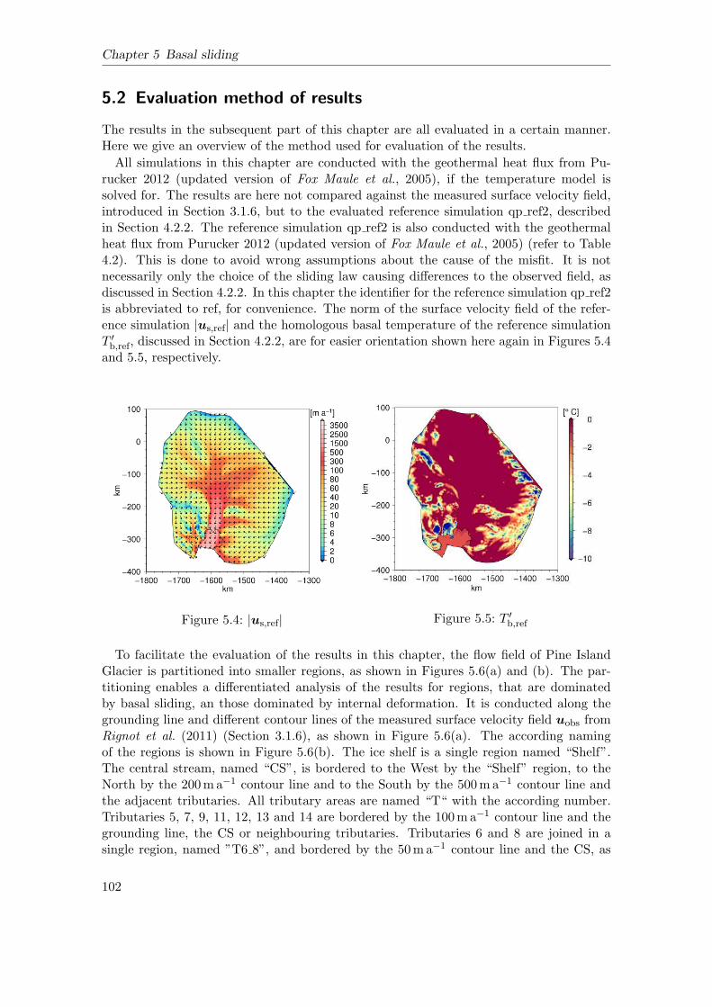
Chapter 5 Basal sliding
5.2 Evaluation method of results
The results in the subsequent part of this chapter are all evaluated in a certain manner.Here we give an overview of the method used for evaluation of the results.
All simulations in this chapter are conducted with the geothermal heat flux from Pu-rucker 2012 (updated version of Fox Maule et al., 2005), if the temperature model issolved for. The results are here not compared against the measured surface velocity field,introduced in Section 3.1.6, but to the evaluated reference simulation qp ref2, describedin Section 4.2.2. The reference simulation qp ref2 is also conducted with the geothermalheat flux from Purucker 2012 (updated version of Fox Maule et al., 2005) (refer to Table4.2). This is done to avoid wrong assumptions about the cause of the misfit. It is notnecessarily only the choice of the sliding law causing differences to the observed field, asdiscussed in Section 4.2.2. In this chapter the identifier for the reference simulation qp ref2is abbreviated to ref, for convenience. The norm of the surface velocity field of the refer-ence simulation |us,ref| and the homologous basal temperature of the reference simulationT ′
b,ref, discussed in Section 4.2.2, are for easier orientation shown here again in Figures 5.4and 5.5, respectively.
Figure 5.4: |us,ref| Figure 5.5: T ′
b,ref
To facilitate the evaluation of the results in this chapter, the flow field of Pine IslandGlacier is partitioned into smaller regions, as shown in Figures 5.6(a) and (b). The par-titioning enables a differentiated analysis of the results for regions, that are dominatedby basal sliding, an those dominated by internal deformation. It is conducted along thegrounding line and different contour lines of the measured surface velocity field uobs fromRignot et al. (2011) (Section 3.1.6), as shown in Figure 5.6(a). The according namingof the regions is shown in Figure 5.6(b). The ice shelf is a single region named “Shelf”.The central stream, named “CS”, is bordered to the West by the “Shelf” region, to theNorth by the 200ma−1 contour line and to the South by the 500ma−1 contour line andthe adjacent tributaries. All tributary areas are named “T“ with the according number.Tributaries 5, 7, 9, 11, 12, 13 and 14 are bordered by the 100ma−1 contour line and thegrounding line, the CS or neighbouring tributaries. Tributaries 6 and 8 are joined in asingle region, named ”T6 8”, and bordered by the 50ma−1 contour line and the CS, as
102

5.2 Evaluation method of results
is tributary 4. Tributary 3 is bordered by the 75ma−1 contour line and the CS. Tribu-taries 1 and 2 are joined, named ”T1 2”, and bordered by the 20ma−1 contour line, theCS and neighbouring tributaries. The same applies to tributary 10. All tributaries, thecentral stream and ice shelf are further combined to the fast flowing region called “Fast”,indicated in red in Figure 5.6(b). The slower flowing region outside the fast streams andthe ice shelf is called “Slow”, indicated in blue in Figure 5.6(b). The “Fast” and “Slow”regions together are combined to the region “All”, which is bordered with a thick blackline in Figure 5.6(b).
The partitioning is somewhat arbitrary, but facilitates nonetheless a differentiated dis-cussion of the results.
(a) (b)
Figure 5.6: Partitioning of regions for evaluation
The results are evaluated on the one hand in a qualitative manner. On the other hand,we also evaluate the root-mean-square deviation RMSus (Eq. (5.8)) for the differentregions. The difference calculated here is between the simulated and reference surfacevelocity fields, such that
RMSus =
√
√
√
√
1
m
m∑
i=1
(||us,sim|i − |uref|i|)2, (5.8)
withm being the number of the discrete values. We evaluate the RMSus value on a regulargrid with 1 km spacing.
The RMSus value enables a quantitative evaluation of the results. In the RMSus value,higher deviations are weighted stronger than in a calculated mean deviation. Further-more, the RMSus value relates to the absolute deviation between the simulations and thereference. The relative misfit is not shown with this measure. In an overall slower flow-ing region therefore the RMSus value is naturally smaller, than in faster flowing regions,assuming the flow pattern in reproduced to some extend. We chose the RMSus deviation,instead of the mean deviation, as a quantitative measure, because it has been used insimilar studies and thus enables comparison (e.g. Joughin et al., 2009; Ruckamp, 2011).
Our aim is to reproduce the surface flow field with all tributaries, by making appropriate
103
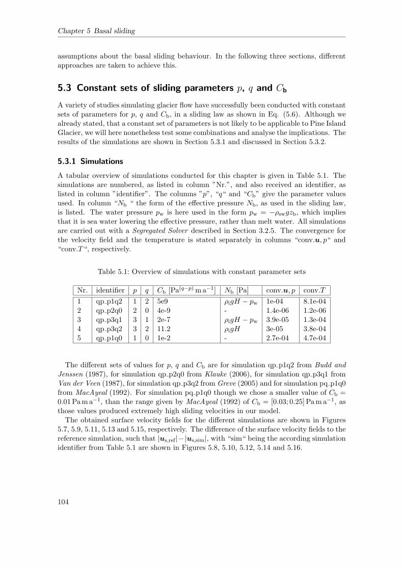
Chapter 5 Basal sliding
assumptions about the basal sliding behaviour. In the following three sections, differentapproaches are taken to achieve this.
5.3 Constant sets of sliding parameters p, q and Cb
A variety of studies simulating glacier flow have successfully been conducted with constantsets of parameters for p, q and Cb, in a sliding law as shown in Eq. (5.6). Although wealready stated, that a constant set of parameters is not likely to be applicable to Pine IslandGlacier, we will here nonetheless test some combinations and analyse the implications. Theresults of the simulations are shown in Section 5.3.1 and discussed in Section 5.3.2.
5.3.1 Simulations
A tabular overview of simulations conducted for this chapter is given in Table 5.1. Thesimulations are numbered, as listed in column ”Nr.”, and also received an identifier, aslisted in column ”identifier”. The columns ”p”, “q“ and “Cb” give the parameter valuesused. In column “Nb “ the form of the effective pressure Nb, as used in the sliding law,is listed. The water pressure pw is here used in the form pw = −ρswgzb, which impliesthat it is sea water lowering the effective pressure, rather than melt water. All simulationsare carried out with a Segregated Solver described in Section 3.2.5. The convergence forthe velocity field and the temperature is stated separately in columns “conv.u, p“ and“conv.T“, respectively.
Table 5.1: Overview of simulations with constant parameter sets
Nr. identifier p q Cb [Pa(q−p)ma−1] Nb [Pa] conv.u, p conv.T
1 qp p1q2 1 2 5e9 ρigH − pw 1e-04 8.1e-042 qp p2q0 2 0 4e-9 - 1.4e-06 1.2e-063 qp p3q1 3 1 2e-7 ρigH − pw 3.9e-05 1.3e-044 qp p3q2 3 2 11.2 ρigH 3e-05 3.8e-045 qp p1q0 1 0 1e-2 - 2.7e-04 4.7e-04
The different sets of values for p, q and Cb are for simulation qp p1q2 from Budd andJenssen (1987), for simulation qp p2q0 from Klauke (2006), for simulation qp p3q1 fromVan der Veen (1987), for simulation qp p3q2 from Greve (2005) and for simulation pq p1q0from MacAyeal (1992). For simulation pq p1q0 though we chose a smaller value of Cb =0.01Pama−1, than the range given by MacAyeal (1992) of Cb = [0.03; 0.25] Pama−1, asthose values produced extremely high sliding velocities in our model.The obtained surface velocity fields for the different simulations are shown in Figures
5.7, 5.9, 5.11, 5.13 and 5.15, respectively. The difference of the surface velocity fields to thereference simulation, such that |us,ref|−|us,sim|, with “sim“ being the according simulationidentifier from Table 5.1 are shown in Figures 5.8, 5.10, 5.12, 5.14 and 5.16.
104
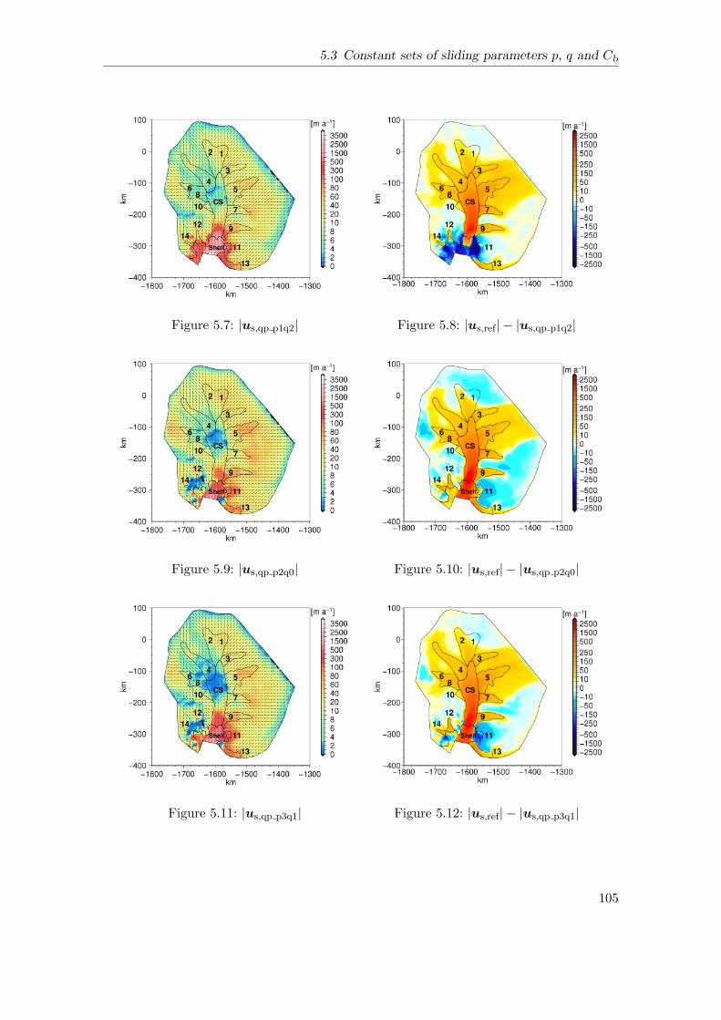
5.3 Constant sets of sliding parameters p, q and Cb
Figure 5.7: |us,qp p1q2| Figure 5.8: |us,ref| − |us,qp p1q2|
Figure 5.9: |us,qp p2q0| Figure 5.10: |us,ref| − |us,qp p2q0|
Figure 5.11: |us,qp p3q1| Figure 5.12: |us,ref| − |us,qp p3q1|
105
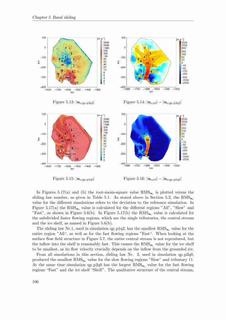
Chapter 5 Basal sliding
Figure 5.13: |us,qp p3q2| Figure 5.14: |us,ref| − |us,qp p3q2|
Figure 5.15: |us,qp p1q0| Figure 5.16: |us,ref| − |us,qp p1q0|
In Figures 5.17(a) and (b) the root-mean-square value RMSus is plotted versus thesliding law number, as given in Table 5.1. As stated above in Section 5.2, the RMSus
value for the different simulations refers to the deviation to the reference simulation. InFigure 5.17(a) the RMSus value is calculated for the different regions ”All”, ”Slow” and”Fast”, as shown in Figure 5.6(b). In Figure 5.17(b) the RMSus value is calculated forthe subdivided faster flowing regions, which are the single tributaries, the central streamand the ice shelf, as named in Figure 5.6(b).
The sliding law Nr.1, used in simulation qp p1q2, has the smallest RMSus value for theentire region ”All“, as well as for the fast flowing regions ”Fast“. When looking at thesurface flow field structure in Figure 5.7, the entire central stream is not reproduced, butthe inflow into the shelf is reasonably fast. This causes the RMSus value for the ice shelfto be smallest, as its flow velocity crucially depends on the inflow from the grounded ice.
From all simulations in this section, sliding law Nr. 2, used in simulation qp p2q0,produced the smallest RMSus value for the slow flowing regions ”Slow” and tributary 11.At the same time simulation qp p2q0 has the largest RMSus value for the fast flowingregions “Fast” and the ice shelf “Shelf”. The qualitative structure of the central stream,
106
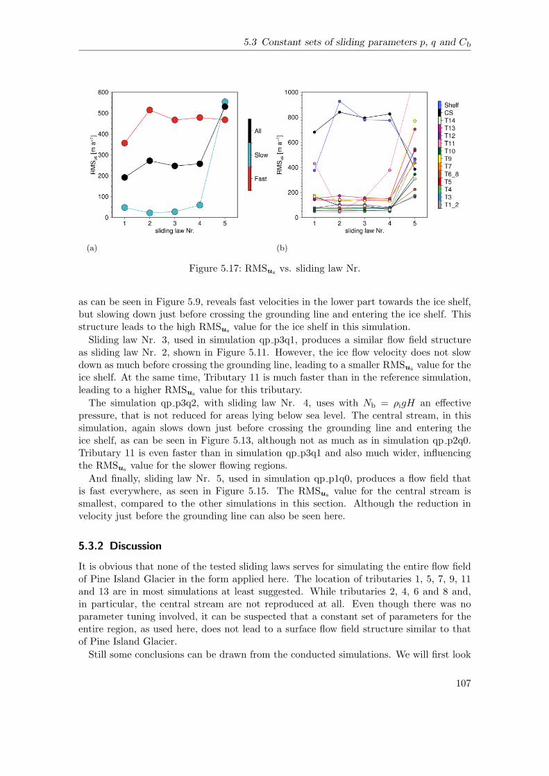
5.3 Constant sets of sliding parameters p, q and Cb
(a) (b)
Figure 5.17: RMSus vs. sliding law Nr.
as can be seen in Figure 5.9, reveals fast velocities in the lower part towards the ice shelf,but slowing down just before crossing the grounding line and entering the ice shelf. Thisstructure leads to the high RMSus value for the ice shelf in this simulation.
Sliding law Nr. 3, used in simulation qp p3q1, produces a similar flow field structureas sliding law Nr. 2, shown in Figure 5.11. However, the ice flow velocity does not slowdown as much before crossing the grounding line, leading to a smaller RMSus value for theice shelf. At the same time, Tributary 11 is much faster than in the reference simulation,leading to a higher RMSus value for this tributary.
The simulation qp p3q2, with sliding law Nr. 4, uses with Nb = ρigH an effectivepressure, that is not reduced for areas lying below sea level. The central stream, in thissimulation, again slows down just before crossing the grounding line and entering theice shelf, as can be seen in Figure 5.13, although not as much as in simulation qp p2q0.Tributary 11 is even faster than in simulation qp p3q1 and also much wider, influencingthe RMSus value for the slower flowing regions.
And finally, sliding law Nr. 5, used in simulation qp p1q0, produces a flow field thatis fast everywhere, as seen in Figure 5.15. The RMSus value for the central stream issmallest, compared to the other simulations in this section. Although the reduction invelocity just before the grounding line can also be seen here.
5.3.2 Discussion
It is obvious that none of the tested sliding laws serves for simulating the entire flow fieldof Pine Island Glacier in the form applied here. The location of tributaries 1, 5, 7, 9, 11and 13 are in most simulations at least suggested. While tributaries 2, 4, 6 and 8 and,in particular, the central stream are not reproduced at all. Even though there was noparameter tuning involved, it can be suspected that a constant set of parameters for theentire region, as used here, does not lead to a surface flow field structure similar to thatof Pine Island Glacier.
Still some conclusions can be drawn from the conducted simulations. We will first look
107
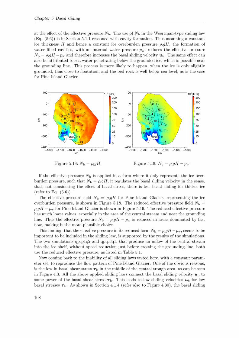
Chapter 5 Basal sliding
at the effect of the effective pressure Nb. The use of Nb in the Weertman-type sliding law(Eq. (5.6)) is in Section 5.1.1 reasoned with cavity formation. Thus assuming a constantice thickness H and hence a constant ice overburden pressure ρigH, the formation ofwater filled cavities, with an internal water pressure pw, reduces the effective pressureNb = ρigH−pw and therefore increases the basal sliding velocity ub. The same effect canalso be attributed to sea water penetrating below the grounded ice, which is possible nearthe grounding line. This process is more likely to happen, when the ice is only slightlygrounded, thus close to floatation, and the bed rock is well below sea level, as is the casefor Pine Island Glacier.
Figure 5.18: Nb = ρigH Figure 5.19: Nb = ρigH − pw
If the effective pressure Nb is applied in a form where it only represents the ice over-burden pressure, such that Nb = ρigH, it regulates the basal sliding velocity in the sense,that, not considering the effect of basal stress, there is less basal sliding for thicker ice(refer to Eq. (5.6)).
The effective pressure field Nb = ρigH for Pine Island Glacier, representing the iceoverburden pressure, is shown in Figure 5.18. The reduced effective pressure field Nb =ρigH − pw for Pine Island Glacier is shown in Figure 5.19. The reduced effective pressurehas much lower values, especially in the area of the central stream and near the groundingline. Thus the effective pressure Nb = ρigH − pw is reduced in areas dominated by fastflow, making it the more plausible choice.
This finding, that the effective pressure in its reduced form Nb = ρigH−pw, seems to beimportant to be included in the sliding law, is supported by the results of the simulations.The two simulations qp p1q2 and qp p3q1, that produce an inflow of the central streaminto the ice shelf, without speed reduction just before crossing the grounding line, bothuse the reduced effective pressure, as listed in Table 5.1.
Now coming back to the inability of all sliding laws tested here, with a constant param-eter set, to reproduce the flow pattern of Pine Island Glacier. One of the obvious reasons,is the low in basal shear stress τ b in the middle of the central trough area, as can be seenin Figure 4.3. All the above applied sliding laws connect the basal sliding velocity ub tosome power of the basal shear stress τ b. This leads to low sliding velocities ub for lowbasal stresses τ b. As shown in Section 4.1.4 (refer also to Figure 4.30), the basal sliding
108
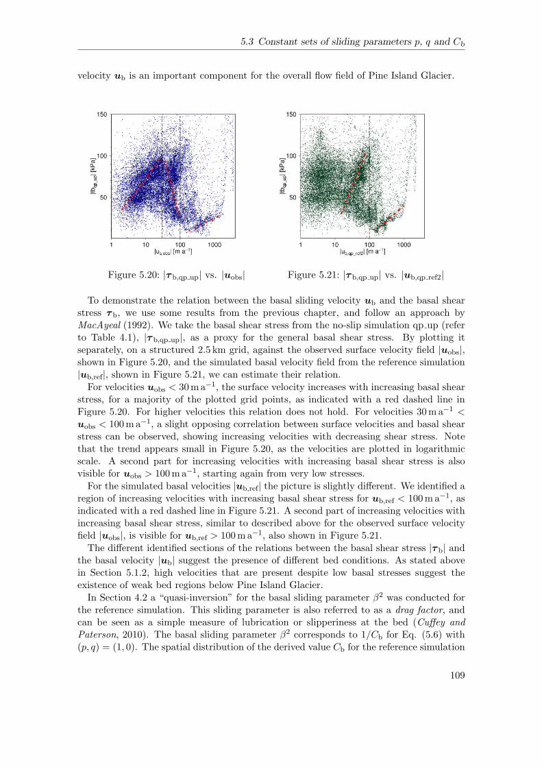
5.3 Constant sets of sliding parameters p, q and Cb
velocity ub is an important component for the overall flow field of Pine Island Glacier.
Figure 5.20: |τ b,qp up| vs. |uobs| Figure 5.21: |τ b,qp up| vs. |ub,qp ref2|
To demonstrate the relation between the basal sliding velocity ub and the basal shearstress τ b, we use some results from the previous chapter, and follow an approach byMacAyeal (1992). We take the basal shear stress from the no-slip simulation qp up (referto Table 4.1), |τ b,qp up|, as a proxy for the general basal shear stress. By plotting itseparately, on a structured 2.5 km grid, against the observed surface velocity field |uobs|,shown in Figure 5.20, and the simulated basal velocity field from the reference simulation|ub,ref|, shown in Figure 5.21, we can estimate their relation.
For velocities uobs < 30ma−1, the surface velocity increases with increasing basal shearstress, for a majority of the plotted grid points, as indicated with a red dashed line inFigure 5.20. For higher velocities this relation does not hold. For velocities 30ma−1 <uobs < 100ma−1, a slight opposing correlation between surface velocities and basal shearstress can be observed, showing increasing velocities with decreasing shear stress. Notethat the trend appears small in Figure 5.20, as the velocities are plotted in logarithmicscale. A second part for increasing velocities with increasing basal shear stress is alsovisible for uobs > 100ma−1, starting again from very low stresses.
For the simulated basal velocities |ub,ref| the picture is slightly different. We identified aregion of increasing velocities with increasing basal shear stress for ub,ref < 100ma−1, asindicated with a red dashed line in Figure 5.21. A second part of increasing velocities withincreasing basal shear stress, similar to described above for the observed surface velocityfield |uobs|, is visible for ub,ref > 100ma−1, also shown in Figure 5.21.
The different identified sections of the relations between the basal shear stress |τ b| andthe basal velocity |ub| suggest the presence of different bed conditions. As stated abovein Section 5.1.2, high velocities that are present despite low basal stresses suggest theexistence of weak bed regions below Pine Island Glacier.
In Section 4.2 a “quasi-inversion” for the basal sliding parameter β2 was conducted forthe reference simulation. This sliding parameter is also referred to as a drag factor, andcan be seen as a simple measure of lubrication or slipperiness at the bed (Cuffey andPaterson, 2010). The basal sliding parameter β2 corresponds to 1/Cb for Eq. (5.6) with(p, q) = (1, 0). The spatial distribution of the derived value Cb for the reference simulation
109
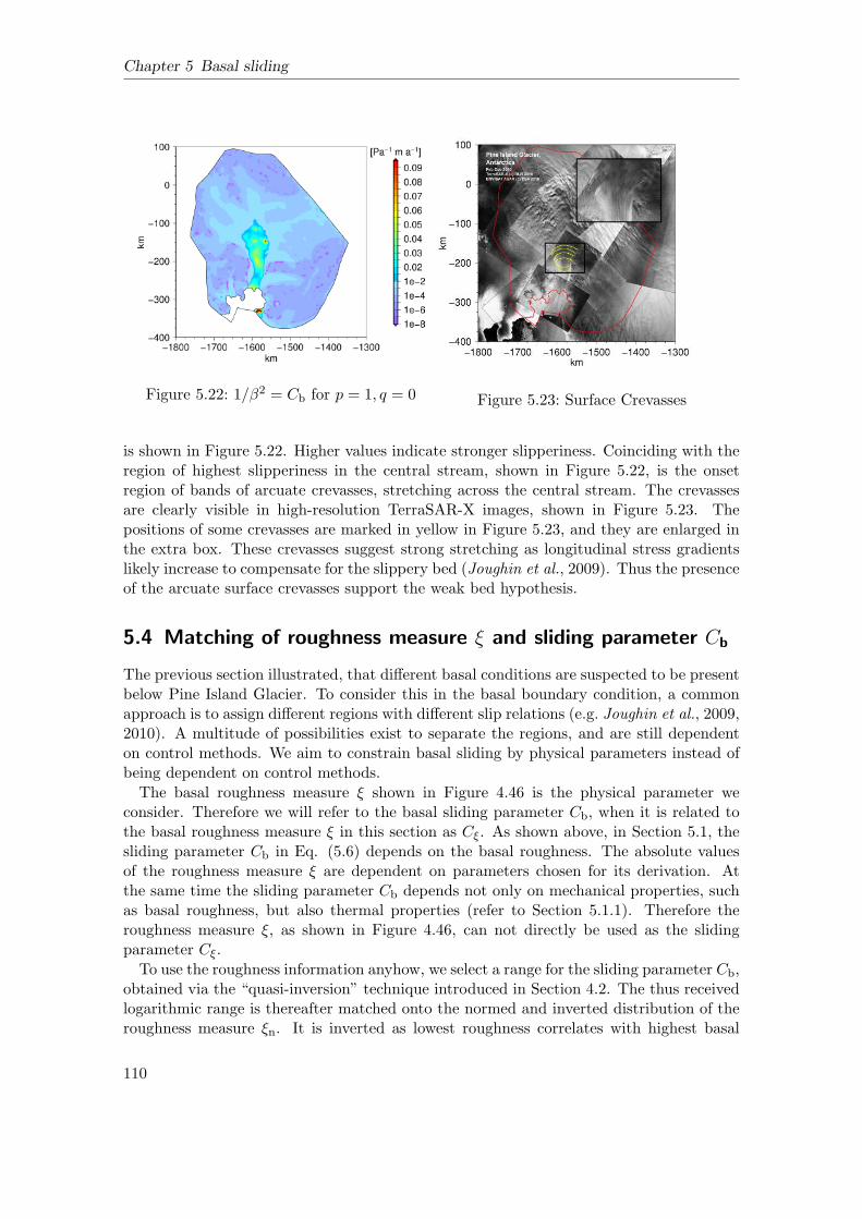
Chapter 5 Basal sliding
Figure 5.22: 1/β2 = Cb for p = 1, q = 0 Figure 5.23: Surface Crevasses
is shown in Figure 5.22. Higher values indicate stronger slipperiness. Coinciding with theregion of highest slipperiness in the central stream, shown in Figure 5.22, is the onsetregion of bands of arcuate crevasses, stretching across the central stream. The crevassesare clearly visible in high-resolution TerraSAR-X images, shown in Figure 5.23. Thepositions of some crevasses are marked in yellow in Figure 5.23, and they are enlarged inthe extra box. These crevasses suggest strong stretching as longitudinal stress gradientslikely increase to compensate for the slippery bed (Joughin et al., 2009). Thus the presenceof the arcuate surface crevasses support the weak bed hypothesis.
5.4 Matching of roughness measure ξ and sliding parameter Cb
The previous section illustrated, that different basal conditions are suspected to be presentbelow Pine Island Glacier. To consider this in the basal boundary condition, a commonapproach is to assign different regions with different slip relations (e.g. Joughin et al., 2009,2010). A multitude of possibilities exist to separate the regions, and are still dependenton control methods. We aim to constrain basal sliding by physical parameters instead ofbeing dependent on control methods.
The basal roughness measure ξ shown in Figure 4.46 is the physical parameter weconsider. Therefore we will refer to the basal sliding parameter Cb, when it is related tothe basal roughness measure ξ in this section as Cξ. As shown above, in Section 5.1, thesliding parameter Cb in Eq. (5.6) depends on the basal roughness. The absolute valuesof the roughness measure ξ are dependent on parameters chosen for its derivation. Atthe same time the sliding parameter Cb depends not only on mechanical properties, suchas basal roughness, but also thermal properties (refer to Section 5.1.1). Therefore theroughness measure ξ, as shown in Figure 4.46, can not directly be used as the slidingparameter Cξ.
To use the roughness information anyhow, we select a range for the sliding parameter Cb,obtained via the “quasi-inversion” technique introduced in Section 4.2. The thus receivedlogarithmic range is thereafter matched onto the normed and inverted distribution of theroughness measure ξn. It is inverted as lowest roughness correlates with highest basal
110
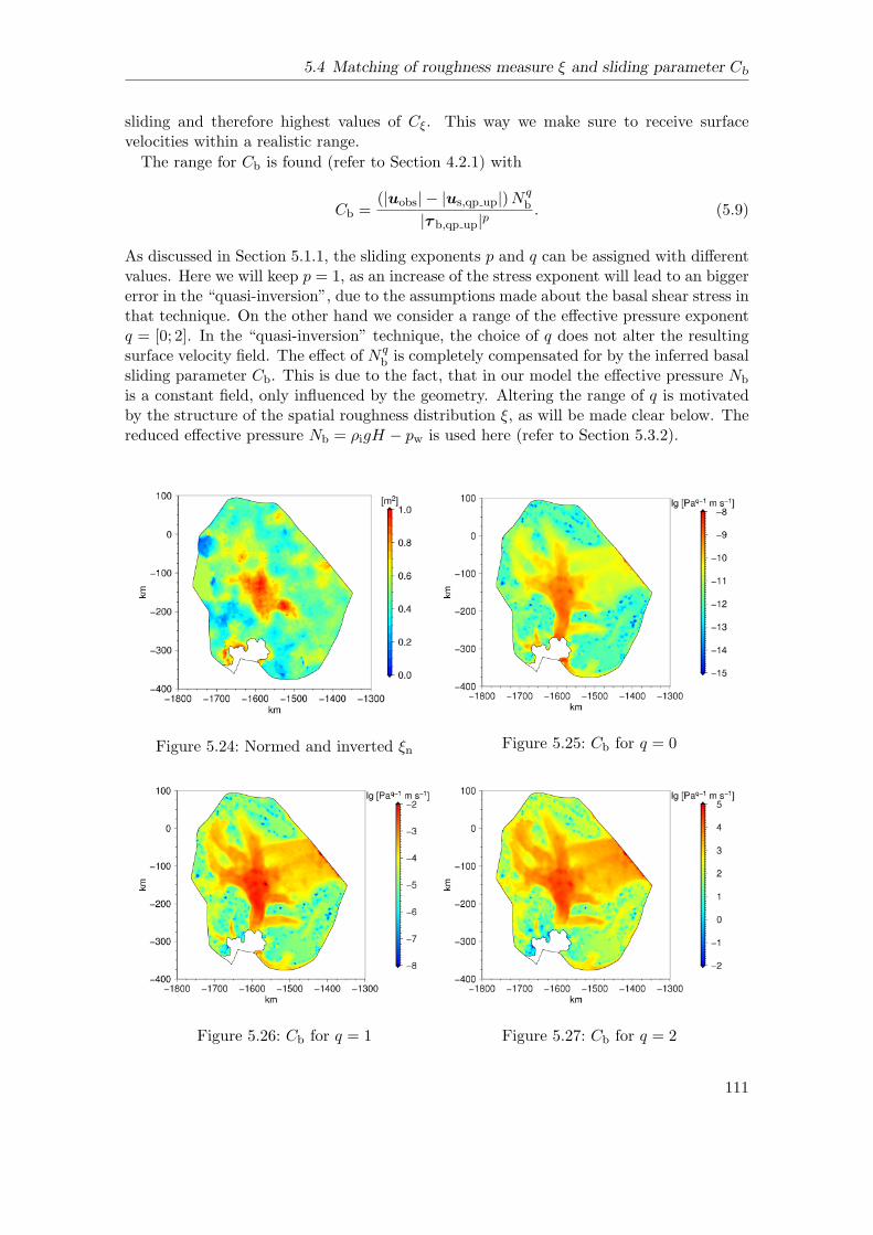
5.4 Matching of roughness measure ξ and sliding parameter Cb
sliding and therefore highest values of Cξ. This way we make sure to receive surfacevelocities within a realistic range.
The range for Cb is found (refer to Section 4.2.1) with
Cb =(|uobs| − |us,qp up|)N
qb
|τ b,qp up|p. (5.9)
As discussed in Section 5.1.1, the sliding exponents p and q can be assigned with differentvalues. Here we will keep p = 1, as an increase of the stress exponent will lead to an biggererror in the “quasi-inversion”, due to the assumptions made about the basal shear stress inthat technique. On the other hand we consider a range of the effective pressure exponentq = [0; 2]. In the “quasi-inversion” technique, the choice of q does not alter the resultingsurface velocity field. The effect of N q
b is completely compensated for by the inferred basalsliding parameter Cb. This is due to the fact, that in our model the effective pressure Nb
is a constant field, only influenced by the geometry. Altering the range of q is motivatedby the structure of the spatial roughness distribution ξ, as will be made clear below. Thereduced effective pressure Nb = ρigH − pw is used here (refer to Section 5.3.2).
Figure 5.24: Normed and inverted ξn Figure 5.25: Cb for q = 0
Figure 5.26: Cb for q = 1 Figure 5.27: Cb for q = 2
111
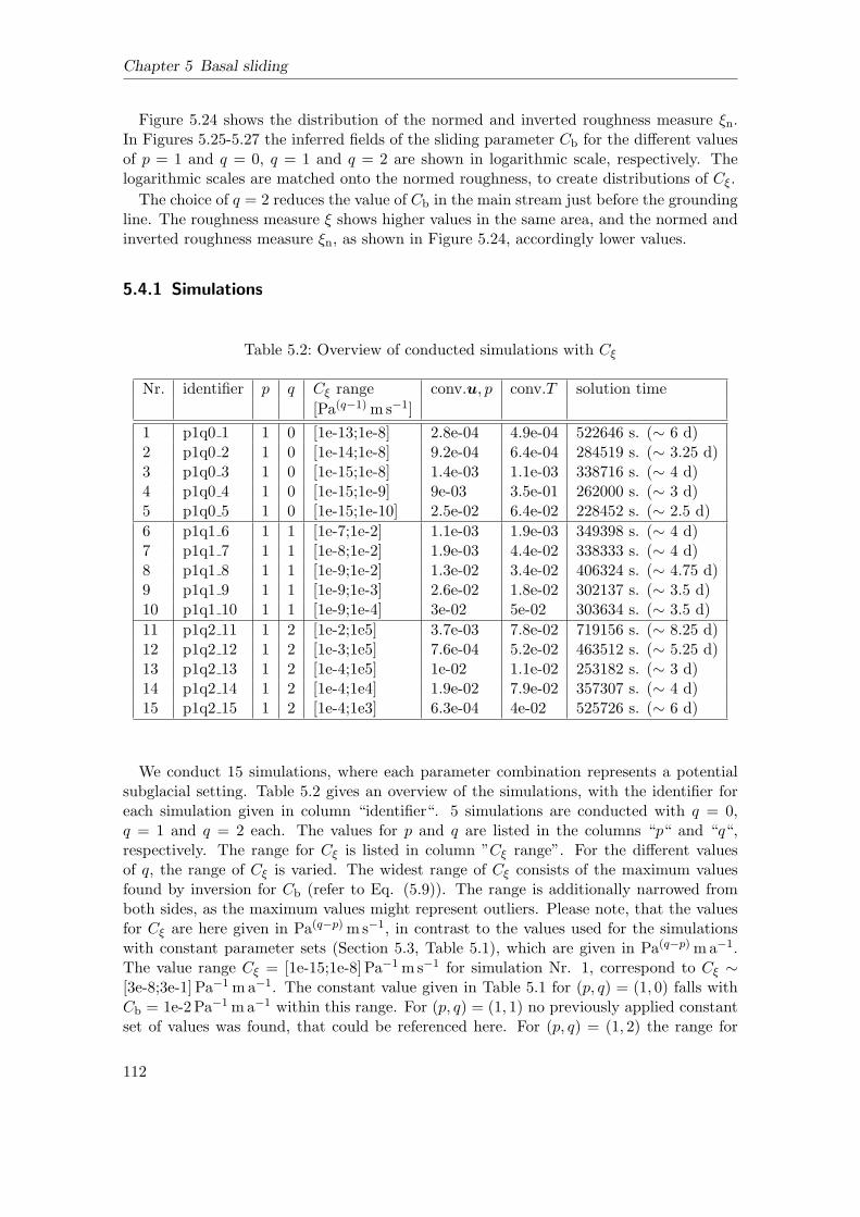
Chapter 5 Basal sliding
Figure 5.24 shows the distribution of the normed and inverted roughness measure ξn.In Figures 5.25-5.27 the inferred fields of the sliding parameter Cb for the different valuesof p = 1 and q = 0, q = 1 and q = 2 are shown in logarithmic scale, respectively. Thelogarithmic scales are matched onto the normed roughness, to create distributions of Cξ.
The choice of q = 2 reduces the value of Cb in the main stream just before the groundingline. The roughness measure ξ shows higher values in the same area, and the normed andinverted roughness measure ξn, as shown in Figure 5.24, accordingly lower values.
5.4.1 Simulations
Table 5.2: Overview of conducted simulations with Cξ
Nr. identifier p q Cξ range conv.u, p conv.T solution time
[Pa(q−1)ms−1]
1 p1q0 1 1 0 [1e-13;1e-8] 2.8e-04 4.9e-04 522646 s. (∼ 6 d)2 p1q0 2 1 0 [1e-14;1e-8] 9.2e-04 6.4e-04 284519 s. (∼ 3.25 d)3 p1q0 3 1 0 [1e-15;1e-8] 1.4e-03 1.1e-03 338716 s. (∼ 4 d)4 p1q0 4 1 0 [1e-15;1e-9] 9e-03 3.5e-01 262000 s. (∼ 3 d)5 p1q0 5 1 0 [1e-15;1e-10] 2.5e-02 6.4e-02 228452 s. (∼ 2.5 d)
6 p1q1 6 1 1 [1e-7;1e-2] 1.1e-03 1.9e-03 349398 s. (∼ 4 d)7 p1q1 7 1 1 [1e-8;1e-2] 1.9e-03 4.4e-02 338333 s. (∼ 4 d)8 p1q1 8 1 1 [1e-9;1e-2] 1.3e-02 3.4e-02 406324 s. (∼ 4.75 d)9 p1q1 9 1 1 [1e-9;1e-3] 2.6e-02 1.8e-02 302137 s. (∼ 3.5 d)10 p1q1 10 1 1 [1e-9;1e-4] 3e-02 5e-02 303634 s. (∼ 3.5 d)
11 p1q2 11 1 2 [1e-2;1e5] 3.7e-03 7.8e-02 719156 s. (∼ 8.25 d)12 p1q2 12 1 2 [1e-3;1e5] 7.6e-04 5.2e-02 463512 s. (∼ 5.25 d)13 p1q2 13 1 2 [1e-4;1e5] 1e-02 1.1e-02 253182 s. (∼ 3 d)14 p1q2 14 1 2 [1e-4;1e4] 1.9e-02 7.9e-02 357307 s. (∼ 4 d)15 p1q2 15 1 2 [1e-4;1e3] 6.3e-04 4e-02 525726 s. (∼ 6 d)
We conduct 15 simulations, where each parameter combination represents a potentialsubglacial setting. Table 5.2 gives an overview of the simulations, with the identifier foreach simulation given in column “identifier“. 5 simulations are conducted with q = 0,q = 1 and q = 2 each. The values for p and q are listed in the columns “p“ and “q“,respectively. The range for Cξ is listed in column ”Cξ range”. For the different valuesof q, the range of Cξ is varied. The widest range of Cξ consists of the maximum valuesfound by inversion for Cb (refer to Eq. (5.9)). The range is additionally narrowed fromboth sides, as the maximum values might represent outliers. Please note, that the valuesfor Cξ are here given in Pa(q−p)ms−1, in contrast to the values used for the simulationswith constant parameter sets (Section 5.3, Table 5.1), which are given in Pa(q−p)ma−1.The value range Cξ = [1e-15;1e-8] Pa−1ms−1 for simulation Nr. 1, correspond to Cξ ∼[3e-8;3e-1] Pa−1ma−1. The constant value given in Table 5.1 for (p, q) = (1, 0) falls withCb = 1e-2Pa−1ma−1 within this range. For (p, q) = (1, 1) no previously applied constantset of values was found, that could be referenced here. For (p, q) = (1, 2) the range for
112
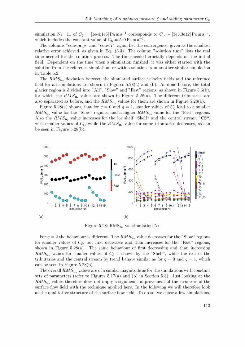
5.4 Matching of roughness measure ξ and sliding parameter Cb
simulation Nr. 11 of Cξ = [1e-4;1e5] Pam s−1 corresponds to Cb ∼ [3e3;3e12] Pama−1,which includes the constant value of Cb = 5e9Pama−1.
The columns ”conv.u, p” and ”conv.T” again list the convergence, given as the smallestrelative error achieved, as given in Eq. (3.3). The column ”solution time” lists the realtime needed for the solution process. The time needed crucially depends on the initialfield. Dependent on the time when a simulation finished, it was either started with thesolution from the reference simulation, or with a solution from another similar simulationin Table 5.2.
The RMSus deviation between the simulated surface velocity fields and the referencefield for all simulations are shown in Figures 5.28(a) and (b). As done before, the totalglacier region is divided into ”All”, ”Slow” and ”Fast” regions, as shown in Figure 5.6(b),for which the RMSus values are shown in Figure 5.28(a). The different tributaries arealso separated as before, and the RMSus values for them are shown in Figure 5.28(b).
Figure 5.28(a) shows, that for q = 0 and q = 1, smaller values of Cξ lead to a smallerRMSus value for the “Slow” regions, and a higher RMSus value for the “Fast” regions.Also the RMSus value increases for the ice shelf “Shelf“ and the central stream ”CS“,with smaller values of Cξ, while the RMSus value for some tributaries decreases, as canbe seen in Figure 5.28(b).
(a) (b)
Figure 5.28: RMSus vs. simulation Nr.
For q = 2 the behaviour is different. The RMSus value decreases for the ”Slow“ regionsfor smaller values of Cξ, but first decreases and than increases for the ”Fast“ regions,shown in Figure 5.28(a). The same behaviour of first decreasing and than increasingRMSus values for smaller values of Cξ is shown by the ”Shelf“, while the rest of thetributaries and the central stream by trend behave similar as for q = 0 and q = 1, whichcan be seen in Figure 5.28(b).The overallRMSus values are of a similar magnitude as for the simulations with constant
sets of parameters (refer to Figures 5.17(a) and (b) in Section 5.3). Just looking at theRMSus values therefore does not imply a significant improvement of the structure of thesurface flow field with the technique applied here. In the following we will therefore lookat the qualitative structure of the surface flow field. To do so, we chose a few simulations,
113

Chapter 5 Basal sliding
which we will analyse in more detail. The ones chosen are not necessarily the ones withthe smallest overall RMSus value, but with interesting features.
Figure 5.29: |us,p1q0 2| Figure 5.30: T ′
b,p1q0 2
Figure 5.29 shows the surface velocity |us,p1q0 2| and Figure 5.30 the homologous basaltemperature T ′
b,p1q0 2 of simulation Nr. 2, with p, q = (1, 0) and Cb = [1e-14;1e-8] Pa−1ms−1.
In the surface velocity field of simulation Nr. 2, the locations of tributaries 7, 11 and 12are well reproduced. The locations of all other tributaries, apart from tributary 8 and 14,are also slightly visible in the surface flow field. In the vicinity of the observed location oftributary 14, the simulation shows an area of ice flowing with high velocities into the iceshelf. A striking feature is, that the velocities in tributary 7 are higher than in the centralstream. The central stream itself flows reasonably fast, but slowing down just beforethe grounding line. This behaviour, as discussed in the last section, does not correlatewith the observations. It leads to higher internal deformation in that region, and thus ahigh strain heating source term ψ. As already mentioned in the last chapter in Section4.2.3, strain heating is the necessary or dominant mechanism to produce a temperate icelayer. The thickness of the temperate ice layer TLT is shown for simulation Nr. 2 inFigure 5.31. A thick temperate ice layer of ∼ 300m is found in the central stream justbefore the grounding line and in the area of tributary 13. The warm ice from within thetemperate layer in the central stream is transported into the shelf, leaving stripes of iceat Tpmp within the shelf (Figure 5.30). The homologous basal temperature T ′
b, as shownin Figure 5.30, reflects the location of most tributaries with a temperate base, such thatT ′
b = 0C. Only tributary 14 is not found at its expected location, as already discussed forthe surface velocity field, shown in Figure 5.29. Tributaries 4, 9, 11, 12 and 13 are, on theother hand, especially clearly separated from the surrounding colder ice by their temperatebases. This feature is even more dominant than in the homologous basal temperature ofthe reference simulation T ′
b,ref, shown in Figure 5.5. This finding is especially interesting,as the tributary locations in the simulation Nr. 2 are not as clearly defined by the surfacevelocity field (Figure 5.29), as is the case for the reference simulation (Figure 5.4).
Figures 5.33 and 5.34 show the surface velocity field |us,p1q1 7| and the homologousbasal temperature T ′
b,p1q1 7, respectively, for simulation Nr. 7, with (p, q) = (1, 1). Theslowing down of the main stream just before the grounding line is not as apparent in this
114

5.4 Matching of roughness measure ξ and sliding parameter Cb
Figure 5.31: TLTp1q0 2 Figure 5.32: TLTp1q2 11
simulation, compared to simulation Nr. 2 (Figure 5.29). The locations of tributaries 7and 11 are clearly visible, while they are not quite as clearly visible for tributaries 5, 9,12 and 13. Tributaries 1, 2, 3, 4, 6, 8, 10 and 14 are not reproduced. Although this is notclearly visible in the RMSus value (Figure 5.28(b)), due to the overall slower velocitiesin those tributaries if < 200ma−1. Tributary 7 shows with a small RMSus value a verygood agreement with the reference simulation. The homologous basal temperature fieldT ′
b,p1q1 7 of simulation Nr. 7 (Figure 5.34) shows a much higher area fraction of temperateice than simulation Nr. 2 (Figure 5.30). Thus the tributaries are not as clearly separated.
Figure 5.33: |us,p1q1 7| Figure 5.34: T ′
b,p1q1 7
Figures 5.35 and 5.36 show the surface velocity field |us,p1q2 11| and the homologousbasal temperature T ′
b,p1q2 11, respectively, for simulation Nr. 11, with (p, q) = (1, 2). Thefeature observed already in the surface velocity of simulation Nr. 7 (Figure 5.33), that themain stream does not slow down before the grounding line as in simulation Nr. 2 (Figure
115
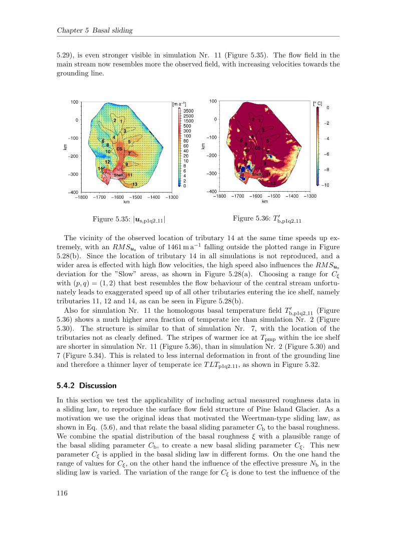
Chapter 5 Basal sliding
5.29), is even stronger visible in simulation Nr. 11 (Figure 5.35). The flow field in themain stream now resembles more the observed field, with increasing velocities towards thegrounding line.
Figure 5.35: |us,p1q2 11| Figure 5.36: T ′
b,p1q2 11
The vicinity of the observed location of tributary 14 at the same time speeds up ex-tremely, with an RMSus value of 1461ma−1 falling outside the plotted range in Figure5.28(b). Since the location of tributary 14 in all simulations is not reproduced, and awider area is effected with high flow velocities, the high speed also influences the RMSus
deviation for the ”Slow” areas, as shown in Figure 5.28(a). Choosing a range for Cξ
with (p, q) = (1, 2) that best resembles the flow behaviour of the central stream unfortu-nately leads to exaggerated speed up of all other tributaries entering the ice shelf, namelytributaries 11, 12 and 14, as can be seen in Figure 5.28(b).
Also for simulation Nr. 11 the homologous basal temperature field T ′
b,p1q2 11 (Figure5.36) shows a much higher area fraction of temperate ice than simulation Nr. 2 (Figure5.30). The structure is similar to that of simulation Nr. 7, with the location of thetributaries not as clearly defined. The stripes of warmer ice at Tpmp within the ice shelfare shorter in simulation Nr. 11 (Figure 5.36), than in simulation Nr. 2 (Figure 5.30) and7 (Figure 5.34). This is related to less internal deformation in front of the grounding lineand therefore a thinner layer of temperate ice TLTp1q2 11, as shown in Figure 5.32.
5.4.2 Discussion
In this section we test the applicability of including actual measured roughness data ina sliding law, to reproduce the surface flow field structure of Pine Island Glacier. As amotivation we use the original ideas that motivated the Weertman-type sliding law, asshown in Eq. (5.6), and that relate the basal sliding parameter Cb to the basal roughness.We combine the spatial distribution of the basal roughness ξ with a plausible range ofthe basal sliding parameter Cb, to create a new basal sliding parameter Cξ. This newparameter Cξ is applied in the basal sliding law in different forms. On the one hand therange of values for Cξ, on the other hand the influence of the effective pressure Nb in thesliding law is varied. The variation of the range for Cξ is done to test the influence of the
116

5.5 Li-sliding
extreme values onto the flow field. The increase of the influence of the effective pressureNb in the sliding law is motivated by the results from Section 5.3, which find the reducedeffective pressure to be important for the flow of Pine Island Glacier (refer to Section5.3.2), as large areas of the base are below sea level.
With the approach presented here we were able to reproduce some of the complexfeatures of the observed surface velocity field of Pine Island Glacier. This effect is notnecessarily represented within the RMSus values shown in Figures 5.28(a) and (b). Thevalues do not differ strongly from the results of the previous section, where constant setsof basal sliding parameters were applied (Section 5.3). However, when looking at theresults in a more qualitative manner, a much better representation of the flow field isapparent. Especially in the simulations Nr. 11-15, with (p, q) = (1, 2), a much betterrepresentation of the central stream and the inflow into the ice shelf across the groundingline is found, than was achieved with a constant set of parameters. The influence of thereduced effective pressure Nb = ρigH−pw is thus emphasised again. At the same time themethod, as applied here, does not lead to a full reproduction of the surface flow structure.This suggests that other processes, not considered here, are also important for the basalsliding behaviour. A possibility not tested yet due to computational constraints is theeffect of the basal stress exponent p. Increasing it would possibly to some extend regulatethe high velocities in some areas, due to low basal stresses (Figure 4.3).
Our results furthermore support our previous finding, that no significant temperate icelayer is suspected in the main stream. Strong basal sliding is necessary for the reproductionof the flow field, which leads to little strain heating, due to lack of internal deformation.
5.5 Li-sliding
The Weertman-type sliding law commonly used in ice flow models, and shown in Eq.(5.6), is based on the idea of regelation and enhanced creep (as shown in Section 5.1),but not really related to these mechanisms anymore. The more parametrised and tunedsliding assumptions were necessary due to complex unknown processes taking place, butalso due to lack of knowledge about the physical composition of the bed itself. Theincreasing availability of RES profiles across Antarctica is changing the latter progressively.RES profiles can be analysed for the basal roughness (refer to Sections 1.1.3 and 4.4).The roughness of the base is becoming increasingly recognised as an important factor inglaciological research (e.g. Rippin et al., 2006). Li et al. (2010) had the idea to bring theoriginal principles of regelation and enhanced creep back into the formulation of the basalsliding law by considering the measured roughness of the bed below the ice.
In this chapter we test the ideas of Li et al. (2010) by application to Pine Island Glacier.In Section 5.5.1 the two-parameter roughness index from Li et al. (2010) is introducedand discussed on the example of Pine Island Glacier. In Section 5.5.2 it is shown howthe original ideas by Weertman (1957) are connected to the ideas by Li et al. (2010),and the sliding relation, as applied in our model, is formulated. And finally, in Section5.5.3, the simulations for Pine Island Glacier with the Li sliding assumption are shownand discussed.
117

Chapter 5 Basal sliding
5.5.1 The two parameter roughness index - ξ2 and η2
A key technique to derive basal roughness are Fourier transformations (FT). A FT canbe used to transform any surface into a sum of several periodically undulated surfaces.This way the amplitude and spatial frequency of the undulations can be expressed. Fortheoretical dynamic studies characterising the roughness by FT works well. However, toshow the spatial distribution of roughness, in a glaciological context, a single parameterindex ξ was introduced (Hubbard et al., 2000; Taylor et al., 2004). The single parameterroughness index ξ is defined as the integral of the spectrum within a specified wavelengthinterval. This method represents the amplitude of the undulations, but information aboutthe frequencies is lost. For Pine Island Glacier the single parameter roughness index ξ wascalculated by Rippin et al. (2011) (Section 4.4) and already used in the previous section(Section 5.4).
Figure 5.37: roughness amplitude ξ2 Figure 5.38: roughness frequency η2
Li et al. (2010) introduce a two-parameter roughness index that represents the amplitudeξ2 and frequency η2 of the undulations. Because of the statistical meanings of ξ2 and η2,they can be used as a proxy for the vertical and horizontal length scales present at the base.To do so the integration interval for ξ2,η2 should be in the metre-scale waveband. Inthe example in Li et al. (2010) they use a moving window length of 1024 points (N = 10,2N = 1024). The spatial resolution is 70m and thus gives a moving window length of∼ 70 km. David Rippin calculated the two-parameter roughness index for Pine IslandGlacier and kindly provided it to us for this study. He first modified his programme so hecould reproduce the values presented in Li et al. (2010) (personal communication, 2012).Still the spatial resolution of the underlain data for Pine Island is different to that of Liet al. (2010). It is calculated with (N = 5, 2N = 32), which is the minimum for N thatshould be used (e.g. Taylor et al., 2004). With a spatial resolution of 34m this leadsto a moving window length of 1088m, which is in the metre-scale waveband required byLi et al. (2010), to be able to apply the data in a sliding relation. Rippin applied theprogramme to Pine Island Glacier and received the fields for ξ2, shown in Figure 5.37 inlogarithmic scale, and for η2, shown in Figure 5.38. The modification of the programmeto reproduce the values of Li et al. (2010) leads to a difference in the total values between
118
5.5 Li-sliding
ξ as shown in Figure 4.46, and ξ2 as shown in Figure 5.37, although the pattern remainsthe same.Li et al. (2010) introduce an interpretation how different basal topographies with their
geomorphic implications can be distinguished from patterns of ξ and η, which is based onideas by Bingham and Siegert (2009). According to this, a marine setting with intensivedeposition and fast and warm ice flow, as proposed for the central part of Pine IslandGlacier, is characterised by low values of ξ and high values of η, thus low-amplitude,low-frequency roughness. This is not necessarily the case for the central trunk area, ascan be seen in Figures 5.37 and 5.38. Instead it seems to be more dominated by low-amplitude, high-frequency roughness, which can be, following Li et al. (2010), interpretedas a continental setting after intensive erosion, also with fast and warm ice flow. Still,this interpretation can not be seen as a contradiction to the earlier stated suspicion ofthe presence of marine sediments. We only considered the relative relation of high andlow values. Absolute values can not be taken here, as they always depend on the spatialresolution of the underlain data, the moving window length and other details for thederivation process of the roughness index.
5.5.2 Assumptions - Controlling obstacle size - Constant CL
To combine the two-parameter roughness index ξ2,η2 with the basal sliding law fromWeertman (1957), Li et al. (2010) state that ξ2 is proportional to the mean square ofamplitudes such that Weertman’s obstacle dimension a can be written as
a = c1 · ξ1/22 , (5.10)
with a proportionality factor c1. The same applies to η2, so that Weertman’s obstaclespacing l can be written as
l = c2 · η1/22 , (5.11)
with a proportionality factor c2.By assuming, that the controlling obstacle size is dominating, as discussed in Section
5.1.1 (Eq. (5.5)), Li et al. (2010) build on the idea of Weertman (1957) and relate the thetwo-parameter roughness index ξ2,η2 to a basal sliding velocity, such that
ub = c
(
η2ξ2
)(n+1)
2
, (5.12)
where c is a factor not depended on geometrical conditions, and n = 3 is the stressexponent (refer Section 2.2.1).To be able to apply the above stated relation as a sliding law, we relate the basal sliding
velocity ub to the basal shear stress τ b, by considering the original approach by Weertman(1957), such that
ub = CL
(
τ bη2ξ2
)(n+1)
2
, (5.13)
with the constant CL = CW(c2/c1)1+n. The value for CW can be estimated, as shown in
Section 5.1.1, and is in our example about CW = 4.46×10⁻²⁹m3 s3 kg−2. The proportion-ality factors c1 and c2 on the other hand are not further defined. Therefore we decided totake CL as a single parameter to adjust.
119
Chapter 5 Basal sliding
To implement the sliding relation, as given in Eq. (5.13), in our model, we need torewrite it in terms of the basal stress τ b, such that
τ b =
(
ub
CL
) 2(n+1)
(
ξ2η2
)
. (5.14)
We estimate a value for CL by assuming, as introduced in Section 4.2.1, the following
CL = (|uobs| − |us,qp up|)|τ b,qp up|−
(n+1)2
(
ξ2η2
)(n+1)
2
. (5.15)
This method does not result in a single value for CL, but in a distribution of values in therange of CL = [6.8e-7;4.3e4] Pa−2ma−1. The maximum and minimum values are herebyonly outliers, while the majority of the values lie within CL = [1e-9; 1e-6] Pa−2ms−1 ∼[3e-2; 3e2] Pa−2ma−1. In the next section we show the simulations conducted with thevalues for CL in the smaller range.
To put the sliding law applied here into context with the previous sections, it can benoted that, with n = 3, Eq. (5.13) represents a Weertman-type sliding law with p = 2and q = 0 (Eq. ( 5.6)), as already discussed in Section 5.1.1 for the controlling obstaclesize ac.
5.5.3 Simulations
For all simulations conducted in this section, only the ice flow model (refer to Section3.2.2) is solved for. The temperature distribution within the ice is taken from the referencesimulation (Section 4.2.2). The base below the fast flowing areas is thus temperate in allsimulations, as can be seen in the distribution of the homologous basal temperature ofthe reference simulation, shown in Figure 5.5. The fully-coupled model is not suitablefor a parameter study, due to time constraints. Use of the temperature field from thereference simulation gives the opportunity to connect the sliding behaviour to the basaltemperature, thus only allowing ice to slide where T is close to Tpmp. This is achievedwith the temperature function f(T ) (refer to Eq. (2.46)), such that the basal boundarycondition is now given as
τ b =
(
ub
CL f(T )
) 2(n+1)
(
ξ2η2
)
. (5.16)
The use of the temperature function f(T ) slightly improves the results shown below, butdoes not change the overall picture.
The simulations conducted vary over CL in the range [1e-9; 1e-6] Pa−2ms−1 ∼ [3e-2; 3e2]Pa−2ma−1, as described above. The RMSus deviations between the reference and simu-lated results are shown for all simulations in Figures 5.39(a) and (b), and show a somewhatregular pattern. For the slower flowing areas, the RMSus value increases with increasingCL, shown in Figure 5.39(a). For the faster flowing areas, the RMSus value first slightlydecreases with increasing CL, and, after reaching a minimum of RMSus = 499.7ma−1 forCL = 1.58Pa−2ma−1, increases with increasing CL. Since we conduct simulations withdiscrete values for CL, the value of RMSus = 499.7ma−1 represents the minimum value forthe simulations conducted here, and not an absolute minimum. The RMSus value for the
120
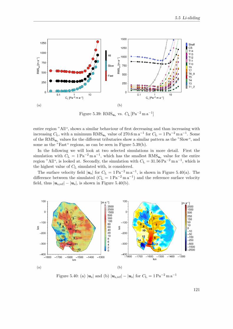
5.5 Li-sliding
(a) (b)
Figure 5.39: RMSus vs. CL [Pa−2ma−1]
entire region ”All“, shows a similar behaviour of first decreasing and than increasing withincreasing CL, with a minimum RMSus value of 270.6ma−1 for CL = 1Pa−2ma−1. Someof the RMSus values for the different tributaries show a similar pattern as the ”Slow“, andsome as the ”Fast“ regions, as can be seen in Figure 5.39(b).
In the following we will look at two selected simulations in more detail. First thesimulation with CL = 1Pa−2ma−1, which has the smallest RMSus value for the entireregion ”All“, is looked at. Secondly, the simulation with CL = 31.56Pa−2ma−1, which isthe highest value of CL simulated with, is considered.
The surface velocity field |us| for CL = 1Pa−2ma−1, is shown in Figure 5.40(a). Thedifference between the simulated (CL = 1Pa−2ma−1) and the reference surface velocityfield, thus |us,ref| − |us|, is shown in Figure 5.40(b).
(a) (b)
Figure 5.40: (a) |us| and (b) |us,ref| − |us| for CL = 1Pa−2ma−1
121

Chapter 5 Basal sliding
Some features of the surface flow field are reproduced, as can be seen in Figure 5.40(a).High velocities are found in the upper part of the central stream. However, the centralstream strongly reduces the speed towards the grounding line. This pattern is even moredominant than in the simulations discussed in the previous sections. Tributaries 2, 4, 5,7, 9, 11 and 13 are reproduced to some extent in the surface flow field, while tributaries1, 3, 6, 8, 10 and 12 are difficult to identify. The area around tributary 14 is, as alsodiscussed in the previous section, dominated by very high velocities. These high velocitiesare also reflected in the difference |us,ref| − |us|, shown in Figure 5.40(b). The groundedarea around tributary 14, as well as the adjacent ice shelf, are dominated by dark bluecolours, representing much higher here simulated velocities, than present in the referencesimulation. This can also be observed in the RMSus value for tributary 14 and CL =1Pa−2ma−1, shown in Figure 5.39(b). The highest RMSus value for this simulation(CL = 1Pa−2ma−1) is found for the ice shelf, which is characterised by strong over- andunderestimation of the surface velocities, compared to the reference simulation (Figure5.40(b)). The second highest RMSus value is found for the central stream, for which thesurface velocity is mainly underestimated.The surface velocity field |us| for CL = 31.56Pa−2ma−1, is shown in Figure 5.41(a).
The difference between the simulated (CL = 31.56Pa−2ma−1) and the reference surfacevelocity field, thus |us,ref| − |us|, is shown in Figure 5.41(b).
(a) (b)
Figure 5.41: (a) |us| and (b) |us,ref| − |us| for CL = 31.56Pa−2ma−1
The surface flow field for CL = 31.56Pa−2ma−1 is dominated by very high velocities(Figure 5.41(b)), which is also reflected in the difference to the reference simulation (Figure5.41(b)), where an overestimation is found in a major part of the entire region. Only thecentral stream area in the vicinity of the grounding line is slower than for the referencesimulation, indicated by the red region in Figure 5.41(b).
This strong overestimation of the velocities is also reflected in the RMSus values inFigures 5.39(a) and (b). On the RMSus values for tributaries 3, 6, 8 and 10 are <500ma−1.
The overall flow pattern can not be reproduced with the method of using the twoparameter roughness index ξ2,η2 in the sliding law. Still some interesting features arise,
122
5.6 Discussion
which will be discussed in the following.
5.5.4 Discussion
In this section we test the applicability of a theory developed by Li et al. (2010) to theregion of Pine Island Glacier, that connects a two parameter roughness index ξ2,η2 tothe basal sliding law. We rewrite the equations from Li et al. (2010), by partly usinginformation of the original ideas from Weertman (1957), and extend the sliding law witha temperature function, to apply it as a boundary condition in our flow model. We definea constant sliding parameter CL, over which a parameter study is conducted.
The results of the surface flow field show certain features. The central stream in allthe simulations from this section is partitioned into a faster flowing upper part, and aslower flowing lower part, in the vicinity of the ice shelf. The speed reduction towards theice shelf was already found in simulations of the preceding two sections, but is here evenstronger pronounced. However, the faster flowing upper part in the simulations conductedhere, resembles much more the observed velocity field, as was the case in the simulationswith constant sets of parameters within the sliding law (Section 5.3).
No single value for CL could be found, that reproduces the surface velocity field of PineIsland Glacier with all its features. For higher CL values, that reproduce the velocitiesin the central stream in a better manner, the velocities in the slower flowing area aroundtributaries 3, 5, 7 and 9, located to the South of the main stream, are simulated muchtoo high (refer to Figure 5.40(a)). Additionally, the area around tributary 14 behavesslightly different to most other tributaries. It speeds up much faster for much lower valuesof CL. This was already found in the previous section, Section 5.4, and is related to thelow roughness measures ξ, ξ2 and η2 in that region.
It has to be noted here, that the method developed by Li et al. (2010), which is basedon the theory from Weertman (1957), is strictly speaking only valid for hard bed sliding,as discussed in Section 5.1.1. Since we showed in Section 5.3.2, that an area of weak bed issuspected below some parts of the central stream of Pine Island Glacier, the method by Liet al. (2010) should strictly speaking not be applied here. Thus it is somewhat surprising,that the method seems to work best in reproducing the surface velocity field in the areaof the suspected weak bed.
Thus, despite the inability of a complete reproduction of the surface flow field of PineIsland Glacier with the method presented here, it still resulted in a surface flow structure,that reveals some important features.
5.6 Discussion
In this chapter we approached the challenge of formulating an appropriate sliding law forthe simulation of the flow field of Pine Island Glacier from 3 different angles. Our startingpoint is hereby always a Weertman-type sliding law, as discussed in Section 5.1.1 andshown in Eq. (5.6).
The first approach, described in Section 5.3, is to take constant sets of sliding parame-ters, that have previously successfully been applied in sliding laws for other areas. Eventhough the flow field structure could not be reproduced with this approach, it let us con-clude, that the reduced effective pressure Nb = ρigH − pw is of major importance for anappropriate sliding law formulation for Pine Island Glacier.
123

Chapter 5 Basal sliding
Our second approach, described in Section 5.4, is based to the original formulation ofthe Weertman-type sliding law, in which the basal sliding parameter Cb is connected to,among other things, the basal roughness. We take a data set of the basal roughness belowPine Island Glacier (Rippin et al., 2011), and match the spatial variation of its field and adefined range of the basal sliding parameter Cb. The procedure is conducted for 3 differentformulations, with a varying impact of the basal effective pressure. The results producea surface flow field, that resembles in its main features the observed field. Although thefingered structure of the tributaries is not as clearly visible, the fast flowing main streamentering the ice shelf, is.
The last approach is based on a method from Li et al. (2010), which they theoreticallydeveloped, and is tested here for its applicability to Pine Island Glacier. The methodrelates a two parameter roughness index ξ2,η2 to the obstacle dimension and spacingof Weertman’s original sliding formulation, described in Section 5.1.1. Simulations areconducted, in which a parameter study over an unconstrained sliding parameter CL iscarried out. The resulting surface flow fields show high velocities in the area of lowdriving stress in the upper central stream. However, the velocity in the lower centralstream reduces towards the grounding line, which contradicts the observed surface velocitypattern.
Figure 5.42: Compilation of RMSus values from the three sections, with the mean valueshown as a filled circle and the range of values shown in the wide bar.
The RMSus deviations from the simulated to the reference surface velocity field arecalculated for all simulations. To distinguish the fast flowing central stream with all itstributaries, which is dominated by basal sliding, as shown in Figure 4.30, from the slowerflowing remainder of the domain, a partitioning is introduced as shown in Figure 5.6(b).The RMSus values for all simulations, subdivided into the regions ”Fast”, ”Slow“ and
124
5.6 Discussion
“All“, are shown in Figure 5.42. The designations ”constant“, ”matched“ and ”li-sliding“refer to the results from Sections 5.3, 5.4 and 5.5, respectively. Each filled circle here refersto the mean value of a region and section, while the coloured bar behind it gives the rangeof values obtained with the according method.The RMSus values, shown in Figure 5.42 thus suggest, that the closest fit of the sim-
ulated to the reference surface velocities is achieved, for all regions ”Fast”, ”Slow“ and“All“, with the method that uses constant sets of parameters, demonstrated in Section5.3. Although, the smallest RMSus values for the ”Slow“ regions are with ∼ 25ma−1,for all 3 methods, very close to each other. The smallest spread of RMSus values, for theregions ”Fast”, ”Slow“ and “All“, is reached with the matching method, treated in Section5.4.The reproduction of the absolute values of the surface flow field, as also discussed in
the previous chapter, in Section 4.2.2, is a challenge. The RMSus values stand for thedeviations to the reproduction. We also already emphasised at various occasions in thischapter, that also the qualitative structure of the flow field is of major importance. Withqualitative structure we mean the reproduction of fast flowing streams and slower flowingregions. So now, stepping away from the error measure of RMSus values, when comparingthe qualitative surface flow field structure, it is by far best reproduced by the matchingmethod, described in Section 5.4.One of the major achievements of this technique is, that it brings some of the original
physical meaning, of representing the basal roughness, back into the sliding law. Theformulation is thus not solely dependent on control methods. This finding is especiallyimportant in a changing basal environment. Smith et al. (2012) describe a process ofrapid subglacial erosion beneath Pine Island Glacier, which could lead to a change in theroughness measure below the glacier. The rapid increase of RES profiles at Pine IslandGlacier make the roughness measure, possibly also the temporal change of it, more widelyavailable.
125


Chapter 6
Conclusions and outlook
The aim of this study was to advance our knowledge about the internal dynamics, basalmotion and thermal structure of Pine Island Glacier, a fast flowing outlet glacier in theWest Antarctic Ice Sheet. The glacier is located in an area of the West Antarctic IceSheet, where the bedrock is in many regions well below the sea level. Additionally, thebed slopes down from the grounding line towards the inland of the glacier. On this kind ofsetting the marine ice sheet instability hypothesis is based, which postulates an intrinsicallyinstable condition Vaughan (2008). In the past decades Pine Island Glacier was observedto have undergone varies changes, including acceleration, thinning and grounding lineretreat. Additionally, rapid subglacial erosion of a marine sediment basin below the glacieris suspected (Smith et al., 2012). The future behaviour of the glacier is important forestimates of global eustatic sea level rise, as Pine Island Glacier alone holds enough iceabove floatation, to raise global sea level by 0.52m, if fully melted (Vaughan et al., 2006).
A variety of external factors can influence the internal dynamics of the glacier, andtherefore being important for its future behaviour. These external factors include thetemperature of the atmosphere at the surface, accumulation, melt rates, the geothermalheat flux at the base and mechanical basal conditions, as for example the existence ofrough bedrock or smooth marine sediments. While the conditions at the surface arenowadays assessable in reasonable temporal and spatial resolution, with use of remotesensing techniques, the conditions at the base still remain widely unknown, due to thedifficult accessibility.
Therefore we aim to define the recent state of important basal conditions at Pine IslandGlacier, with use of a thermo-mechanically coupled 3D full-Stokes ice flow model. Inglacier dynamic studies, the coupling of the temperature field to the flow dynamics is ofhigh importance. Higher internal ice temperatures lead to a stronger internal deformation.Additionally, as ice is believed to slide over its base only at interface temperatures nearor at the local melting point, the sliding behaviour is also sensitively influenced by thetemperature distribution. Furthermore, the consideration of all stress terms, as done inthe here presented full-Stokes model, is especially important when simulating processesin the vicinity of the grounding line. The coupled ice flow model is implemented inthe commercial Finite Element Method software COMSOL Multiphysics©. The softwareCOMSOL has previously already been successfully applied to the study of glaciologicalquestions (e.g. Humbert, 2010; Ruckamp, 2011). We advanced and extended the applicationto a coupled ice sheet - ice shelf system in three dimensions. The implementation andvalidation of the coupled flow model is conducted as part of this study.
The results of the application of the validated coupled flow model to the region ofPine Island Glacier, are divided into two parts. In the first part, the dominant localmechanisms driving the flow of Pine Island Glacier are investigated. This is of interest
127

Chapter 6 Conclusions and outlook
because the surface flow field is dominated by a complex structure of various tributariesfeeding into a fast flowing main stream. In a changing environment, the tributaries mightreact differently to external changes. Additionally the information can be of interest forplanning of measurement surveys in the area. Our results are validated along the observedsurface velocity field of Pine Island Glacier, representing the surface flow structure in theyears 2007 to 2009 (Rignot et al., 2011). We carefully declare our results to be a likelypresent setting, as the complex glacial system can not uniquely be defined with a diagnosticexperimental set up (Raymond and Gudmundsson, 2009). Still we can exclude unlikely,and emphasise the more likely settings. To our knowledge it is the first full-Stokes flowmodel to successfully solve fully-coupled for the glacier flow and temperature field of PineIsland Glacier in three dimensions.
Our results show, that large areas at the base of the glacier are temperate, with tem-peratures at the pressure melting point. At the same time the thickness of the temperatebasal layer is suspected to be very small in most areas. Only the area around a smalltributary feeding into the ice shelf, tributary 11, shows a wider area of a temperate layerthickness > 70m. Tributaries 4 and 6, feeding into the upper part of the central stream,are separated by a band of cold ice at the base, suggesting a temperature control of theflow field in that area. In some fast streaming areas the finding of a temperate base isstrongly coupled to the inclusion of a friction heating term. This could suggest supportof a deceleration, if initiated due to other factors, like for example a change in the basalmechanical conditions in that area. An increased geothermal heat flux around the locationof a suspected sub volcanic centre below Pine Island Glacier (Corr and Vaughan, 2008) isnot suspected to alter the flow structure significantly, as the structure of the temperateice at the base seems to be reasonably stable in our simulations. This is not including theeffect of change in the effective pressure, who’s importance will be emphasised below. Weidentify the data set from Purucker 2012 (updated version of Fox Maule et al., 2005) forthe geothermal heat flux below Pine Island Glacier to be the likely best representation ofactual conditions.
Basal sliding is identified to be the dominant mechanism for fast flow at Pine IslandGlacier. Formulation of an appropriate sliding law to be used as a basal boundary con-dition in ice flow models is one of the big challenges in present numerical glaciologicalstudies. Therefore, in the second part of this study, we focus on the formulation of an ap-propriate sliding law for Pine Island Glacier. As a starting point, we test the applicabilityof formulations, that have been successfully applied in other areas. These formulationsconsist of constant parameter sets in a Weertman-type sliding law. The results show, thata reduced effective pressure is necessary to be included in the basal sliding law, to simulatethe transition from grounded to floating ice in the central stream appropriately. All testedformulations with constant parameter sets though are not able to reproduce the upperpart of the fast flowing central stream, and generally the fingered structure of the flowfield. This is partly due to an area with very low basal stress in the middle of the centralstream, where a Weertman-type sliding law with constant parameter sets can not producehigh basal velocities. This challenge is usually met by the use of control methods, thatproduce a spatially varying basal sliding parameter, accounting for the differences in thesurface flow field. Our reference simulation was conducted with a similar approach. Ina next step we want to include a measured physical quantity into the formulation of thebasal sliding law.
The structure of the low in driving stress partially correlates with the structure of the
128

basal roughness below Pine Island Glacier, as derived by Rippin et al. (2011). Thereforea marine sediment basin is likely present, where weak till can not support the basal dragof the fast flowing ice, being in a state of plastic failure. This motivates our attempt toinclude some of the original physical meaning of the basal sliding parameter Cb in a slidinglaw, by matching the structure of the basal roughness with a relevant range of values. Theresults show a much better representation of the surface flow field, with a fast flowingcentral stream. Although, an area of very low roughness adjacent to the slow flowing partof the ice shelf, leads to an overestimation of flow velocities in that area. The method weintroduce here, thus, although promising, needs to be extended to include other locallyrelevant factors, to reproduce the observed surface velocity field at Pine Island Glacier. Animportant role hereby can likely be tributed to the subglacial water system, not modelledexplicitly in this study. The importance of the effective pressure in a sliding formulationemphasises this.Another method of including information about the basal roughness in the basal sliding
formulation is based on a theory by Li et al. (2010). This theory relates a two parameterroughness index, representing the amplitude and frequency of the roughness, to Weert-man’s original obstacle dimension and spacing. The thus formulated sliding law, whichleaves one parameter to adjust, is applied to Pine Island Glacier. The resulting flow fieldstructure shows high velocities in the upper part of the central stream, but low velocitiesin the lower part, towards the ice shelf. The sliding law, as formulated here, does notinclude the effective water pressure yet.As an outlook for interesting questions to be addressed in the future, we will in the
following make some suggestions. The fully coupled ice flow model should be extendedeven further. Shear margins should be included in the ice flow model, connecting damagewith the enhancement factor. Also the connection of basal roughness and sliding should beanalysed further. The Li-sliding formulation should be extended with the effective waterpressure. Possibly the speed reduction in the central stream towards the ice shelf could beregulated. In the future it would be worthwhile to couple a hydrological model to it, as theeffective pressure was shown to be very important to the sliding behaviour. Additionally,the internal deformation of the underlying till could be modelled explicitly. Also theimplementation of grounding line motion is meaningful. If successfully included, prognosticstudies could be conducted. The prognostic studies would focus on decadal changes,as the full-Stokes model is not applicable to much longer periods due to computationalconstraints. For Pine Island Glacier this is of interest, as changes are observed evenin a decadal time scale. The thermal state, especially in the region where a significanttemperate layer was found, could be verified with help of RES profiles.We want to conclude with a few final remarks. The present state of the internal tem-
perature and flow structure of Pine Island Glacier was successfully simulated. The resultsshow a predominantly cold glacier, with a big part of the base being temperate. The flowfield in the central stream and the numerous tributaries is dominated by basal sliding.Our formulation of the basal sliding law emphasises the connection between sliding ve-locity and basal roughness, as parts of the complex observed surface flow structure couldbe reproduced. The present dynamics and temperature structure of the glacier are ofmajor importance for its future behaviour. A thermo-mechanically coupled model, as wepresented here, is essential for the inference of interrelations between the thermal regime,the basal roughness structure and the flow and sliding conditions.
129

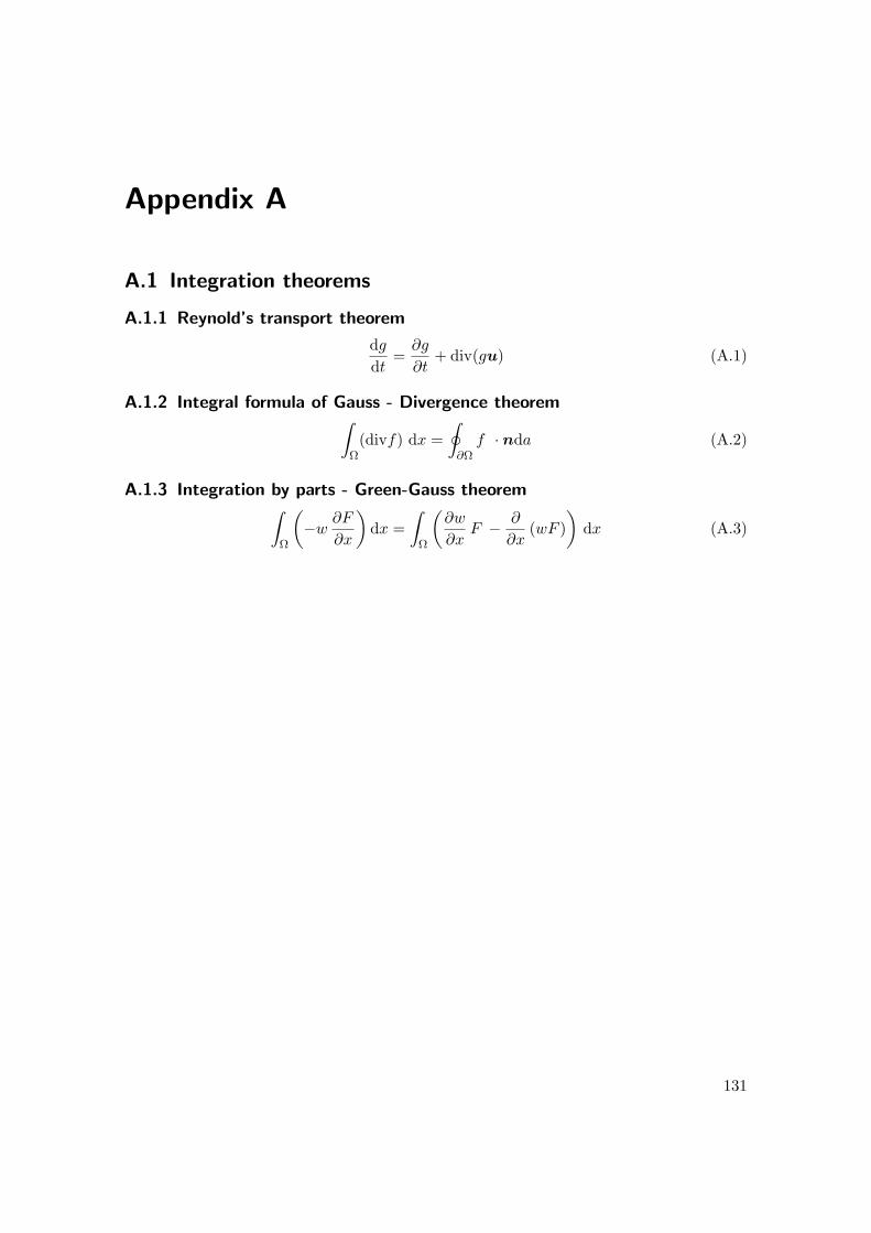
Appendix A
A.1 Integration theorems
A.1.1 Reynold’s transport theorem
dg
dt=∂g
∂t+ div(gu) (A.1)
A.1.2 Integral formula of Gauss - Divergence theorem∫
Ω(divf) dx =
∮
∂Ωf · nda (A.2)
A.1.3 Integration by parts - Green-Gauss theorem∫
Ω
(
−w∂F
∂x
)
dx =
∫
Ω
(
∂w
∂xF −
∂
∂x(wF )
)
dx (A.3)
131

Bibliography
Alley, R., 1992: Flow-law hypotheses for ice-sheet modeling. J. Glaciol, 38(129), 245–256.
Alley, R. B., I. Joughin, et al., 2012: Modeling ice-sheet flow. Science, 336(6081), 551–552.
Aschwanden, A., E. Bueler, C. Khroulev, and H. Blatter, 2012: An enthalpy formulationfor glaciers and ice sheets. Journal of Glaciology, 58(209), 441–457.
Bamber, J. L., J. L. Gomez-Dans, , and J. A. Griggs, 2009: A new 1km digital elevationmodel of the Antarctic derived from combined satellite radar and laser data – Part 1:Data and methods. The Cryosphere, 3, 101–111.
Bamber, J. L., R. E. M. Riva, B. L. A. Vermeersen, and A. M. LeBrocq, 2009: Reassess-ment of the Potential Sea-Level Rise from a Collapse of the West Antarctic Ice Sheet.Science, 324, 901–903.
Baral, D. R., K. Hutter, and R. Greve, 2001: Asymptotic Theories of Large-Scale Mo-tion, Temperature, and Moisture Distribution in Land-Based Polythermal Ice Sheets:A Critical Review and New Developments. Applied Mechanics Reviews, 54, 215.
Barnes, P., D. Tabor, and J. Walker, 1971: The friction and creep of polycrystalline ice.Proceedings of the Royal Society of London. A. Mathematical and Physical Sciences,324(1557), 127–155.
Benn, D. I. and D. J. A. Evans, 2010: Glaciers and Glaciation. Hodder Arnold Publication,2nd edition.
Bentley, C. R. and N. A. Ostenso, 1961: Glacial and subglacial topography of WestAntarctica. Journal of Glaciology, 3(29), 882–912.
Bindschadler, R., 1983: The importance of pressurized subglacial water in separation andsliding at the glacier bed. Journal of Glaciology, 29(101), 3–19.
Bindschadler, R., 2006: The environment and evolution of the West Antarctic ice sheet:setting the stage. Philosophical Transactions of the Royal Society A, 364, 1583–1605.
Bindschadler, R. A., 2002: History of lower Pine Island Glacier, West Antarctica, fromLandsat imagery. Journal of Glaciology, 48(163), 536–544.
Bingham, R. G., E. C. King, A. M. Smith, and H. D. Pritchard, 2010: Glacial geomor-phology: Towards a convergence of glaciology and geomorphology. Progress in PhysicalGeography, 34(3), 327–355.
Bingham, R. G. and M. J. Siegert, 2009: Quantifying subglacial bed roughness in Antarc-tica: implications for ice-sheet dynamics and history. Quaternary Science Reviews,28(3-4), 223–236.
133
Bibliography
Bjornsson, H., 1988: Hydrology of ice caps in volcanic regions.
Blankenship, D., R. Bell, S. Hodge, J. Brozena, J. Behrendt, and C. Finn, 1993: Activevolcanism beneath the West Antarctic ice sheet and implications for ice-sheet stability.
Blatter, H., 1995: Velocity and stress fields in grounded glaciers: a simple algorithm forincluding deviatoric stress gradients. Journal of Glaciology, 41(138), 333–344.
Blatter, H., R. Greve, and A. Abe-Ouchi, 2010: A short history of the thermomechanicaltheory and modelling of glaciers and ice sheets. Journal of Glaciology, 56(200), 1087–1094.
Blatter, H. and K. Hutter, 1991: Polythermal conditions in Arctic glaciers. Journal ofGlaciology, 37(126), 261–269.
Bohlander, J. and T. Scambos, 2007: Antarctic coastlines and grounding line derivedfrom MODIS Mosaic of Antarctica (MOA). National Snow and Ice Data Center. Digitalmedia. Accessed 24 April 2008., Boulder, Colorado USA.
Bougamont, M., S. Tulaczyk, and I. Joughin, 2003: Response of subglacial sedimentsto basal freeze-on 2. Application in numerical modeling of the recent stoppage of IceStream C, West Antarctica. Journal of Geophysical Research, 108(B4), 2223.
Boulton, G. and R. Hindmarsh, 1987: Sediment deformation beneath glaciers: rheologyand geological consequences. Journal of Geophysical Research, 92(B9), 9059–9082.
Boulton, G. S. and D. Dent, 1974: The nature and rates of post-depositional changes inrecently deposited till from south-east iceland. Geografiska Annaler. Series A. PhysicalGeography 121–134.
Boulton, G. S. and A. S. Jones, 1979: Stability of temperate ice caps and ice sheets restingon beds of deformable sediment. Journal of Glaciology, 24, 29–43.
Budd, W. and T. Jacka, 1989: A review of ice rheology for ice sheet modelling. ColdRegions Science and Technology, 16(2), 107–144.
Budd, W. and D. Jenssen, 1987: Numerical modelling of the large-scale basal water fluxunder the West Antarctic Ice Sheet. In Dynamics of the West Antarctic Ice Sheet,Van der Veen, C.J., O. J., editor. Kluwer, Dordrecht, 293–320.
Bueler, E., 2008: Lessons from the short history of ice sheet model intercomparison. TheCryosphere Discussions, 2(3), 399–412.
Bueler, E., J. Brown, and C. Lingle, 2007: Exact solutions to the thermomechanicallycoupled shallow ice approximation: effective tools for verification. Journal of Glaciology,53(182), 499–516.
Christoffersen, P. and S. Tulaczyk, 2003: Response of subglacial sediments to basal freeze-on 1. Theory and comparison to observations from beneath the West Antarctic Ice Sheet.Journal of Geophysical Research, 108(B4), 2222.
Clarke, G., 1987: A short history of scientific investigations on glaciers. Journal ofGlaciology 4–24.
134

Bibliography
Clarke, G., 2005: Subglacial processes. Annual Review of Earth and Planetary Sciences,33, 247–276.
Clarke, G., G. Cross, and C. Benson, 1989: Radar imaging of glaciovolcanic stratigra-phy, Mount Wrangell caldera, Alaska: interpretation model and results. Journal ofGeophysical Research, 94(B6), 7237–7249.
Comiso, J. C., 2000: Variability and Trends in Antarctic Surface Temperatures from InSitu and Satellite Infrared Measurements. Journal of Climate, 13, 1674–1696.
COMSOL, 2008: COMSOL Multiphysics Reference Guide. COMSOL AB, Vers. 3.5a.
COMSOL, 2012a: COMSOL Multiphysics Reference Guide. COMSOL AB, Vers. 4.3a.
COMSOL, 2012b: COMSOL Multiphysics User’s Guide. COMSOL AB, Vers. 4.3a.
Cornford, S., D. Martin, D. Graves, D. Ranken, A. Le Brocq, R. Gladstone, A. Payne,E. Ng, and W. Lipscomb, 2012: Adaptive mesh, finite volume modeling of marine icesheets. Journal of Computational Physics 529–549.
Corr, H. F. J., C. S. M. Doake, A. Jenkins, and D. G. Vaughan, 2001: Investigations ofan ”ice plain” in the mouth of Pine Island Glacier, Antarctica. Journal of Glaciology,47(156), 51–57.
Corr, H. F. J. and D. G. Vaughan, 2008: A recent volcanic eruption beneath the WestAntarctic ice sheet. Nature Geoscience, 1(2), 122–125.
Cuffey, K. M. and W. S. B. Paterson, 2010: The Physics of Glaciers. Butterworth-Heinemann, 4th edition.
Dahl-Jensen, D., N. Gundestrup, S. Gogineni, and H. Miller, 2003: Basal melt at North-GRIP modeled from borehole, ice-core and radio-echo sounder observations. Annals ofGlaciology, 37(1), 207–212.
Dalziel, I. W. D. and D. H. Elliot, 1982: West Antarctica: Problem child of Gondwanaland.Tectonics, 1(1), 3–19.
Dalziel, I. W. D. and L. A. Lawver, 2001: The lithospheric setting of the West Antarcticice sheet. The West Antarctic Ice Sheet: Behavior and Environment, 77, 29–44.
Deeley, R. M. and P. H. Parr, 1914: The Hintereis Glacier. Philosophical Magazine, 27,153–176.
Dierckx, M. and J.-L. Tison, 2013: Marine ice deformation experiments: an empiricalvalidation of creep parameters. Geophysical Research Letters 1–5.
Docquier, D., L. Perichon, and F. Pattyn, 2011: Representing Grounding Line Dynamicsin Numerical Ice Sheet Models: Recent Advances and Outlook. Surveys in Geophysics,32, 417–435.
Durand, G., O. Gagliardini, B. de Fleurian, T. Zwinger, and E. L. Meur, 2009: Marine Ice-Sheet Dynamics: Hysteresis and Neutral Equilibrium. Journal of Geophysical Research,114, F03009.
135

Bibliography
Durand, G., O. Gagliardini, L. Favier, T. Zwinger, and E. le Meur, 2011: Impact ofbedrock description on modeling ice sheet dynamics. Geophysical Research Letters,38(20), L20501.
Durand, G., O. Gagliardini, T. Zwinger, E. L. Meur, and R. C. A. Hindmarsh, 2009: Full-Stokes modeling of marine ice-sheets: influence of the grid size. Annals of Glaciology,50(52), 109–114.
Durran, D. R., 2010: Numerical methods for fluid dynamics: With applications to geo-physics, volume 32. Springer.
Duval, P., 1977: The role of the water content on the creep rate of polycrystalline ice.Isotopes and impurities in snow and ice, 118, 29–33.
Echelmeyer, K., 1987: Direct observation of basal sliding and deformation of basal driftat sub-freezing temperatures. Journal 0/Claciology, 33(113).
Echelmeyer, K. A., W. D. Harrison, C. Larsen, and J. E. Mitchell, 1994: The role ofthe margins in the dynamics of an active ice stream. Journal of Glaciology, 40(136),527–538.
Engelhardt, H., 2004: Ice temperature and high geothermal flux at Siple Dome, WestAntarctica, from borehole measurements. Journal of Glaciology, 50(169), 251–256.
Engelhardt, H., N. Humphrey, B. Kamb, and M. Fahnestock, 1990: Physical conditionsat the base of a fast moving Antarctic ice stream. Science, 248, 57–59.
Engelhardt, H. and B. Kamb, 1998: Basal sliding of ice stream B, West Antarctica.Journal of Glaciology, 44(147), 223–230.
Favier, L., O. Gagliardini, G. Durand, and T. Zwinger, 2012: A three-dimensional fullStokes model of the grounding line dynamics: effect of a pinning point beneath the iceshelf. The Cryosphere, 6(1), 101–112.
Flowers, G. E., H. Bjornsson, and F. Palsson, 2003: New insights into the subglacialand periglacial hydrology of Vatnajokull, Iceland, from a distributed physical model.Journal of Glaciology, 49(165), 257–270.
Fowler, A. C., 1986: A sliding law for glaciers of constant viscosity in the presence ofsubglacial cavitation. Proceedings of the Royal Society of London. A. Mathematical andPhysical Sciences, 407(1832), 147–170.
Fox Maule, C., M. E. Purucker, N. Olsen, and K. Mosegaard, 2005: Heat Flux Anomaliesin Antarctica Revealed by Satellite Magnetic Data. Science, 309(5733), 464 – 467.
Fretwell, P., H. Pritchard, D. Vaughan, J. Bamber, N. Barrand, R. Bell, C. Bianchi,R. Bingham, D. Blankenship, G. Casassa, et al., 2013: Bedmap2: improved ice bed,surface and thickness datasets for Antarctica. The Cryosphere Discussions, 7, 376–393.
Gagliardini, O., D. Cohen, P. Raback, and T. Zwinger, 2007: Finite-element modeling ofsubglacial cavities and related friction law. Journal of Geophysical Research, 112(F2),F02027.
136
Bibliography
Gagliardini, O., F. Gillel-Chaulet, and M. Montagnat, 2009: A review of anisotropicpolar ice models: from crystal to ice-sheet flow models. Low Temperature Science,68(Supplement), 149–166.
Gladstone, R. M., V. Lee, J. Rougier, A. J. Payne, H. Hellmer, A. L. Brocq, A. Shepherd,T. L. Edwards, J. Gregory, and S. L. Cornford, 2012: Calibrated prediction of PineIsland Glacier retreat during the 21st and 22nd centuries with a coupled flowline model.Earth and Planetary Science Letters, 333-334, 191–199.
Gladstone, R. M., V. Lee, A. Vieli, and A. J. Payne, 2010: Grounding line migration inan adaptive mesh ice sheet model. Journal of Geophysical Research, 115(F4), F04014.
Gladstone, R. M., A. J. Payne, and S. L. Cornford, 2012: Resolution requirements forgrounding-line modelling: sensitivity to basal drag and ice-shelf buttressing. Annals ofGlaciology, 53(60), 97–105.
Glen, J., 1952: Experiments on the deformation of ice. Journal of Glaciology, 2, 111–114.
Glen, J. W., 1955: The creep of polycrystalline ice. Proceedings of the Royal Society ofLondon. A. Mathematical and Physical Sciences, 228(1175), 519–538.
Gramelsberger, G., 2010: Computerexperimente - Zum Wandel der Wissenschaft imZeitalter des Computers. transcript Verlag, Bielefeld.
Greve, R., 1997: Application of a polythermal three-dimensional ice sheet model to theGreenland ice sheet: response to steady-state and transient climate scenarios. Journalof Climate, 10(5), 901–918.
Greve, R., 2005: Relation of measured basal temperatures and the spatial distributionof the geothermal heat flux for the Greenland ice sheet. Annals of Glaciology, 42(1),424–432.
Greve, R. and H. Blatter, 2009: Dynamics of ice sheets and glaciers. Springer.
Groh, A., H. Ewert, M. Scheinert, M. Fritsche, A. Rulke, A. Richter, R. Rosenau, andR. Dietrich, 2012: An Investigation of Glacial Isostatic Adjustment over the AmundsenSea Sector, West Antarctica. Global and Planetary Change, 98-99, 45–53.
Gudmundsson, G. H., 2003: Transmission of basal variability to a glacier surface. Journalof Geophysical Research, 108(B5), 2253.
Gudmundsson, G. H., 2011: Ice-stream response to ocean tides and the form of the basalsliding law. The Cryosphere, 5, 259–270.
Gudmundsson, G. H., J. Krug, G. Durand, L. Favier, and O. Gagliardini, 2012: Thestability of grounding lines on retrograde slopes. The Cryosphere Discussions, 6, 2597–2619.
Hindmarsh, R. C. A., 1993: Qualitative dynamics of marine ice sheets. Ice in the ClimateSystem I, 12, 68–99.
Hindmarsh, R. C. A., 1996: Stability of ice rises and uncoupled marine ice sheets. Annalsof Glaciology, 23, 94–104.
137
Bibliography
Holland, D. M. and A. Jenkins, 1999: Modeling thermodynamic ice-ocean interactions atthe base of an ice shelf. Journal of Physical Oceanography, 29(8), 1787–1800.
Hooke, R., 1981: Flow law for polycrystalline ice in glaciers: comparison of theoreticalpredictions, laboratory data, and field measurements. Reviews of Geophysics, 19(4),664–672.
Hooke, R. L., 2005: Principles of Glacier Mechanics. Cambridge University Press.
Horwath, M. and R. Dietrich, 2009: Signal and error in mass change inferences fromGRACE: the case of Antarctica. Geophysical Journal International, 177, 849–864.
Hubbard, B., M. Siegert, and D. McCarroll, 2000: Spectral roughness of glaciated bedrockgeomorphic surfaces: implications for glacier sliding. Journal of Geophysical Research,105(B9), 21295–21303.
Hughes, T., 1973: Is the West Antarctic ice sheet disintegrating? Journal of GeophysicalResearch, 78(33), 7884–7910.
Hughes, T. J., 2000: The finite element method: linear static and dynamic finite elementanalysis. Dover Publications.
Humbert, A., 2006: Numerical simulations of the ice flow dynamics of Fimbulisen. FRISPReport, 17, 67–78.
Humbert, A., 2010: The temperature regime of Fimbulisen, Antarctica. Annals of Glaciol-ogy, 51(55), 56–64.
Humbert, A., T. Kleiner, C. Mohrholz, C. Oelke, R. Greve, and M. Lange, 2009: Acomparative modeling study of the Brunt Ice Shelf/Stancomb-Wills Ice Tongue system,East Antarctica. Journal of Glaciology, 55(189), 53–65.
Hutter, K., 1983: Theoretical glaciology: material science of ice and the mechanics ofglaciers and ice sheets. Reidel.
Hutter, K. and K. Johnk, 2004: Continuum methods of physical modeling: continuummechanics, dimensional analysis, turbulence. Springer.
Huybrechts, P. and J. de Wolde, 1999: The dynamic response of the Greenland andAntarctic ice sheets to multiple-century climatic warming. Journal of Climate, 12(8),2169–2188.
Iken, A., 1981: The effect of the subglacial water pressure on the sliding velocity of aglacier in an idealized numerical model. Journal of Glaciology, 27, 407–421.
IPCC-AR3, 2001: The scientific basis. Contribution of working group I to the third assess-ment report of the Intergovernmental Panel on Climate Change. Cambridge UniversityPress: Cambridge, United Kingdom.
IPCC-AR4, 2007: Contribution of Working Group I to the Fourth Assessment Re-port of the Intergovernmental Panel on Climate Change. Cambridge UniversityPress,Cambridge, United Kingdom and New York, NY, USA,.
138
Bibliography
Jacka, T. and W. Budd, 1989: Isotropic and anisotropic flow relations for ice dynamics.Annals of Glaciology, 12, 81–84.
Jacobs, S. S., H. H. Hellmer, and A. Jenkins, 1996: Antarctic ice sheet melting in theSoutheast Pacific. Geophysical Research Letters, 23(9), 957–960.
Jacobs, S. S., A. Jenkins, C. F. Giulivi, and P. Dutrieux, 2011: Stronger ocean circulationand increased melting under Pine Island Glacier ice shelf. Nature Geoscience, 4, 519–523.
Jamieson, S. S., A. Vieli, S. J. Livingstone, C. O. Cofaigh, C. Stokes, C.-D. Hillenbrand,and J. A. Dowdeswell, 2012: Ice-stream stability on a reverse bed slope. Nature Geo-science, 5, 799–802.
Jenkins, A., P. Dutrieux, S. S. Jacobs, S. D. McPhail, J. R. Perrett, A. T.Webb, andD. White, 2010: Observations beneath Pine Island Glacier in West Antarctica andimplications for its retreat. Nature Geoscience, 3(7), 468–472.
Johnson, C., 2009: Numerical Solution of Partial Differential Equations by the FiniteElement Method. Dover Publications, Inc., Mineola, New York.
Jordan, T., F. Ferraccioli, D. Vaughan, J. Holt, H. Corr, D. Blankenship, and T. Diehl,2009: Aerogravity evidence for major crustal thinning under the Pine Island Glacierregion (West Antarctica). Geological Society of America Bulletin, 122(5–6), 714–726.
Joughin, I. and R. B. Alley, 2011: Stability of the West Antarctic ice sheet in a warmingworld. Nature Geoscience, 4, 506–513.
Joughin, I., D. R. MacAyeal, and S. Tulaczyk, 2004: Basal shear stress of the Ross icestreams from control method inversions. Journal of Geophysical Research, 109(B9),1–62.
Joughin, I., B. E. Smith, and D. M. Holland, 2010: Sensitivity of 21st century sea levelto ocean-induced thinning of Pine Island Glacier, Antarctica. Geophysical ResearchLetters, 37, L20502.
Joughin, I. R., E. Rignot, C. E. Rosanova, B. K. Lucchitta, and J. Bohlander, 2003:Timing of Recent Accelerations of Pine Island Glacier, Antarctica. Geophysical ResearchLetters, 30(13), 28–31.
Joughin, I. R., S. Tulaczyk, J. L. Bamber, D. D. Blankenship, J. W. Holt, T. A. Scambos,and D. G. Vaughan, 2009: Basal conditions for Pine Island and Thwaites Glaciers,West Antarctica, determined using satellite and airborne data. Journal of Glaciology,55(190), 245–257.
Kamb, B., 1970: Sliding motion of glaciers: theory and observations. Reviews of Geo-physics and Space Physics, 8(4), 673–728.
Kamb, B., 2001: Basal zone of the west Antarctic ice streams and its role in lubrication oftheir rapid motion. In The West Antarctic Ice Sheet, behavior and environment, Alley,R. B. and Bindschadler, R. A., editors. AGU, 157-199.
139

Bibliography
Karlsson, N. B., D. M. Rippin, D. G. Vaughan, and H. F. J. Corr, 2009: The internallayering of Pine Island Glacier, West Antarctica, from airborne radar-sounding data.Annals of Glaciology, 50, 141–146.
Katz, R. F. and M. G. Worster, 2010: Stability of ice-sheet grounding lines. Proceedingsof the Royal Society A: Mathematical, Physical and Engineering Science, 466(2118),1597–1620.
King, E. C., J. Woodward, and A. M. Smith, 2004: Seismic evidence for a water-filled canalin deforming till beneath Rutford Ice Stream, West Antarctica. Geophysical Researchletters, 31(20), L20401.
Klauke, S., 2006: Numerische Modellierung eines Antarktischen Eisschild-Schelfeis-Systems- Riiser-Larsen und Einzugsgebiet. Master’s thesis.
Kleiner, T., 2010: Entwicklung eines dreidimensionalen numerischen full-Stokes-Fließmodells und seine Anwendung auf ein Inland-Schelfeissystem der Antarktis imBereich des westlichen Droning Maud Lands. PhD thesis, Universitat Munster.
Kleiner, T. and A. Humbert, 2014: Numerical simulations of major ice streams in westernDronning Maud Land, Antarctica, under wet and dry basal conditions. Journal ofGlaciology, 60(220), 215–232.
Landvik, J. Y., S. Bondevik, A. Elverhoi, W. Fjeldskaar, J. Mangerud, O. Salvigsen,M. Siegert, J. Svendsen, and T. Vorren, 1998: The last glacial maximum of Svalbardand the Barents Sea area: ice sheet extent and configuration. Quaternary ScienceReviews, 17(1-3), 43–75.
Langel, R. and W. Hinze, 1998: The magnetic field of the earth’s lithosphere: the satelliteperspective. Cambridge University Press.
Larour, E., J. Schiermeier, E. Rignot, H. Seroussi, M. Morlighem, and J. Paden, 2012:Sensitivity Analysis of Pine Island Glacier ice flow using ISSM and DAKOTA. Journalof Geophysical Research, 117(F2), F02009.
Le Brocq, A. M., A. J. Payne, and A. Vieli, 2010: An improved Antarctic dataset for highresolution numerical ice sheet models (ALBMAP v1). Earth System Science Data.
Leng, W., L. Ju, M. Gunzburger, and S. Price, 2013: Manufactured solutions and theverification of three-dimensional Stokes ice-sheet models. The Cryosphere, 7, 19–29.
Lestringant, R., 1994: A two-dimensional finite-element study of flow in the transitionzone between an ice sheet and an ice shelf. Annals of Glaciology, 20(1), 67–72.
Li, X., B. Sun, M. J. Siegert, R. G. Bingham, X. Tang, D. Zhang, X. Cui, and X. Zhang,2010: Characterization of subglacial landscapes by a two-parameter roughness index.Journal of Glaciology, 56(199), 831–836.
Lliboutry, L., 1968: General theory of subglacial cavitation and sliding of temperateglaciers. Journal of Glaciology, 7, 21–58.
140
Bibliography
Lliboutry, L., 1971: Permeability, brine content and temperature of temperate ice. Journalof Glaciology, 10, 15–29.
Lliboutry, L., 1987: Very Slow Flows of Solids: Basics of modeling in geodynamics andglaciology. Martinus Nijhoff.
Lliboutry, L., 1993: Internal melting and ice accretion at the bottom of temperate glaciers.Journal of Glaciology, 39, 50–64.
Lliboutry, L. and P. Duval, 1985: Various isotropic and anisotropic ices found in glaciersand polar ice caps and their corresponding rheologies. 3(2), 207–224.
MacAyeal, D. R., 1989: Large-scale ice flow over a viscous basal sediment- Theory andapplication to ice stream B, Antarctica. Journal of Geophysical Research, 94(B4), 4071–4087.
MacAyeal, D. R., 1992: The basal stress distribution of Ice Stream E, Antarctica, inferredby control methods. Journal of Geophysical Research, 97(B1), 595–603.
MacGregor, J. A., G. A. Catania, M. S. Markowski, and A. G. Andrews, 2012: Widespreadrifting and retreat of ice-shelf margins in the eastern Amundsen Sea Embayment between1972 and 2011. Journal of Glaciology, 58(209), 458–466.
Mercer, J., 1978: West Antarctic ice sheet and CO2 greenhouse effect- A threat of disaster.Nature, 271(5643), 321–325.
Millero, F., 1978: Freezing point of sea water. Eighth Report of the Joint Panel onOceanographic Tables and Standards. UNESCO, Paris.
Morland, L., 1984: Thermomechanical balances of ice sheet flows. Geophysical & Astro-physical Fluid Dynamics, 29(1-4), 237–266.
Morland, L., 1987: Unconfined ice-shelf flow. Dynamics of the West Antarctic Ice Sheet99–116.
Morlighem, M., 2011: Ice sheet porperties inferred by combining numerical modeling andremote sensing data. PhD thesis, Ecole Centrale Paris.
Morlighem, M., E. Rignot, H. Seroussi, E. Larour, H. Ben Dhia, and D. Aubry, 2010:Spatial patterns of basal drag inferred using control methods from a full-Stokes andsimpler models for Pine Island Glacier, West Antarctica. Geophysical Research Letters,37(14), L14502.
Mothes, H., 1926: Dickenmessungen von Gletschereis mit seismischen Methoden. Geolo-gische Rundschau, 17(6), 397–400.
Naish, T., R. Powell, R. Levy, G. Wilson, R. Scherer, F. Talarico, L. Krissek, F. Niessen,M. Pompilio, T. Wilson, L. Carter, R. DeConto, P. Huybers, R. McKay, D. Pollard,J. Ross, D. Winter, P. Barrett, et al., 2009: Obliquity-paced Pliocene West Antarcticice Sheet oscillations. Nature, 458, 322–328.
Nerem, R. S., E. Leuliette, and A. Cazenave, 2006: Present-day sea-level change: Areview. Comptes Rendus Geoscience, 338(14), 1077–1083.
141

Bibliography
Nitsche, F., S. Jacobs, R. Larter, and K. Gohl, 2007: Bathymetry of the Amundsen Seacontinental shelf: Implications for geology, oceanography, and glaciology. GeochemistryGeophysics Geosystems, 8, Q10009.
Nye, J., 1953: The flow law of ice from measurements in glacier tunnels, laboratoryexperiments and the Jungfraufirn borehole experiment. Proceedings of the Royal Societyof London. A. Mathematical and Physical Sciences, 219(1139), 477–489.
Nye, J., 1957: The distribution of stress and velocity in glaciers and ice-sheets. Proceedingsof the Royal Society of London. A. Mathematical and Physical Sciences, 239(1216), 113–133.
Nye, J. F., 1969: The calculation of sliding of ice over a wavy surface using Newtonianviscous approximation. Proceedings of the Royal Society, London, A311(1506), 445–467.
Park, J., N. Gourmelen, A. Shepherd, S. Kim, D. Vaughan, and D. Wingham, 2013:Sustained retreat of the Pine Island Glacier. Geophysical Research Letters, 40, 1–6.
Paterson, W., 1994: The physics of glaciers. Oxford, etc., Elsevier.
Pattyn, F., 2000: Ice-sheet modelling at different spatial resolutions: focus on the ground-ing zone. Annals of Glaciology, 31(1), 211–216.
Pattyn, F., 2003: A new three-dimensional higher-order thermomechanical ice sheetmodel: Basic sensitivity, ice stream development, and ice flow across subglacial lakes.Journal of Geophysical Research, 108(B8), 2382.
Pattyn, F. and G. Durand, 2013: Why marine ice sheet model predictions may diverge inestimating future sea level rise. Geophysical Research Letters, 40, 4316–4320.
Pattyn, F., L. Perichon, A. Aschwanden, B. Breuer, B. de Smedt, O. Gagliardini, G. H.Gudmundsson, R. C. A. Hindmarsh, A. Hubbard, J. V. Johnson, T. Kleiner, Y. Kono-valov, C. Martin, A. J. Payne, D. Pollard, S. Price, M. Ruckamp, F. Saito, O. Soucek,S. Sugiyama, and T. Zwinger, 2008: Benchmark experiments for higher-order and full-Stokes ice sheet models (ISMIP-HOM). The Cryosphere, 2, 95–108.
Pattyn, F., L. Perichon, G. Durand, L. Favier, O. Gagliardini, R. Hindmarsh, T. Zwinger,T. Albrecht, S. Conford, D. Docquier, H. Gudmundsson, A. Humbert, T. Kleiner,E. Larour, D. Martin, M. Morlighem, A. Payne, M. Ruckamp, N. Wilkens, et al., 2013:Grounding-line migration in plan-view marine ice-sheet models: results of the ice2seaMISMIP3d intercomparison. Journal of Glaciology, 59(215), 2163.
Pattyn, F., C. Schoof, L. Perichon, R. Hindmarsh, E. Bueler, B. de Fleurian, G. Durand,O. Gagliardini, R. Gladstone, D. Goldberg, et al., 2012: Results of the Marine Ice SheetModel Intercomparison Project, MISMIP. The Cryosphere, 6(3), 573–588.
Payne, A. J. and D. J. Baldwin, 2000: Analysis of ice-flow instabilities identified in theEISMINT intercomparison exercise. Annals of Glaciology, 30(1), 204–210.
Payne, A. J., A. Vieli, A. P. Shepherd, D. J. Wingham, and E. Rignot, 2004: Recent dra-matic thinning of the largest West Antarctic ice stream triggered by oceans. GeophysicalResearch Letters, 31, L23401.
142
Bibliography
Peters, M. E., D. D. Blankenship, and D. L. Morse, 2005: Analysis techniques for co-herent airborne radar sounding: Application to West Antarctic ice streams. Journal ofGeophysical Research, 110(B6), B06303.
Pettersson, R., P. Jansson, and H. Blatter, 2004: Spatial variability in water content atthe cold-temperate transition surface of the polythermal Storglaciaren, Sweden. Journalof Geophysical Research, 109(F2), F02009.
Pfeffer, W. T., J. Harper, and S. O’Neel, 2008: Kinematic constraints on glacier contri-butions to 21st-century sea-level rise. Science, 321(5894), 1340–1343.
Pollack, H., S. Hurter, and J. Johnson, 1993: Heat flow from the Earth’s interior: analysisof the global data set. Reviews of Geophysics, 31(3), 267–280.
Pollard, D. and R. DeConto, 2012: A simple inverse method for the distribution of basalsliding coefficients under ice sheets, applied to Antarctica. The Cryosphere Discussions,6, 1405–1444.
Pollard, D. and R. M. DeConto, 2009: Modelling West Antarctic ice sheet growth andcollapse through the past five million years. Nature, 458, 329–332.
Pralong, A., 2005: On the instability of hanging glaciers. PhD thesis, Swiss FederalInstitute of Technology, Zurich.
Pritchard, H., S. Ligtenberg, H. Fricker, D. Vaughan, M. Van den Broeke, and L. Padman,2012: Antarctic ice-sheet loss driven by basal melting of ice shelves. Nature, 484(7395),502–505.
Raymond, M. J. and G. H. Gudmundsson, 2009: Estimating basal properties of ice streamsfrom surface measurements: a non-linear Bayesian inverse approach applied to syntheticdata. The Cryosphere, 3(2), 265–278.
Reddy, J. and D. Gartling, 2010: The finite element method in heat transfer and fluiddynamics. CRC.
Rignot, E., 2001: Evidence for rapid retreat and mass loss of Thwaites Glacier, WestAntarctica. Journal of Glaciology, 47(157), 213–222.
Rignot, E., 2002: Ice-shelf changes in Pine Island Bay, Antarctica, 1947-2000. Journal ofGlaciology, 48(161), 256.
Rignot, E., 2006: Changes in ice dynamics and mass balance of the Antarctic ice sheet.Philosophical Transactions of the Royal Society A, 364, 1637–1655.
Rignot, E., 2008: Changes in West Antarctic ice stream dynamics observed with ALOSPALSAR data. Geophysical Research Letters, 35(12), L12505.
Rignot, E., J. Mouginot, and B. Scheuchl, 2011: Ice flow of the Antarctic ice sheet.Science, 333(6048), 1427–1430.
Rignot, E. J., 1998: Fast recession of a West Antarctic glacier. Science, 281(5376),549–551.
143
Bibliography
Rippin, D., J. Bamber, M. Siegert, D. Vaughan, and H. Corr, 2006: Basal conditions be-neath enhanced-flow tributaries of Slessor Glacier, East Antarctica. Journal of Glaciol-ogy, 52(179), 481–490.
Rippin, D., D. Vaughan, and H. Corr, 2011: The basal roughness of Pine Island Glacier,West Antarctica. Journal of Glaciology, 57(201), 67–76.
Ruckamp, M., 2011: Eisgeometrie und Fließdynamik der subpolaren Eiskappe von KingGeorge Island (Antarktis). PhD thesis, Universitat Munster.
Scambos, T. A., J. Bohlander, C. Shuman, and P. Skvarca, 2004: Glacier accelerationand thinning after ice shelf collapse in the larsen b embayment, antarctica. GeophysicalResearch Letters, 31(18), L18402.
Scherer, R. P., A. Aldahan, S. Tulaczyk, G. Possnert, H. Engelhardt, and B. Kamb, 1998:Pleistocene Collapse of the West Antarctic Ice Sheet. Science, 281, 82–85.
Schmeltz, M., E. Rignot, T. K. Dupont, and D. R. Macayeal, 2002: Sensitivity of PineIsland Glacier, West Antarctica, to changes in ice-shelf and basal conditions: a modelstudy. Journal of Glaciology, 48(163), 552–558.
Schoof, C., 2005: The effect of cavitation on glacier sliding. Proceedings of the RoyalSociety A: Mathematical, Physical and Engineering Science, 461(2055), 609–627.
Schoof, C., 2007a: Ice sheet grounding line dynamics: Steady states, stability, and hys-teresis. Journal of Geophysical Research, 112, F03S28.
Schoof, C., 2007b: Marine ice-sheet dynamics. Part 1. The case of rapid sliding. Journalof Fluid Mechanics, 573, 27–56.
Schweizer, J., 1989: Friction at the base of a glacier. Mitteilungen der Versuchsanstaltfuer Wasserbau, Hydrologie und Glaziologie der ETH Zuerich, 101.
Scott, J. B. T., G. H. Gudmundsson, A. M. Smith, R. G. Bingham, H. D. Pritchard, andD. G. Vaughan, 2009: Increased rate of acceleration on Pine Island Glacier stronglycoupled to changes in gravitational driving stress. The Cryosphere, 3, 125–131.
Seddik, H., R. Greve, T. Zwinger, F. Gillet-Chaulet, and O. Gagliardini, 2012: Simulationsof the Greenland ice sheet 100 years into the future with the full Stokes model Elmer/Ice.Journal of Glaciology, 58(209), 427–440.
Sergienko, O., R. Bindschadler, P. Vornberger, and D. MacAyeal, 2008: Ice stream basalconditions from block-wise surface data inversion and simple regression models of icestream flow: Application to Bindschadler Ice Stream. Journal of Geophysical Research,113(F4), F04010.
Shapiro, N. M. and M. H. Ritzwoller, 2004: Inferring surface heat flux distributions guidedby a global seismic model: particular application to Antarctica. Earth and PlanetaryScience Letters, 223, 213–224.
Shepherd, A., E. R. Ivins, A. Geruo, V. R. Barletta, M. J. Bentley, S. Bettadpur, K. H.Briggs, D. H. Bromwich, R. Forsberg, N. Galin, et al., 2012: A Reconciled Estimate ofIce-Sheet Mass Balance. Science, 338(6111), 1183–1189.
144
Bibliography
Shepherd, A. P., D. J. Wingham, and E. Rignot, 2004: Warm ocean is eroding WestAntarctic Ice Sheet. Geophysical Research Letters, 31, L23402.
Shreve, R., 1972: Movement of water in glaciers. J. Glaciol, 11(62), 205–214.
Smith, A., C. Bentley, R. Bingham, and T. Jordan, 2012: Rapid subglacial erosion beneathPine Island Glacier, West Antarctica. Geophysical Research Letters, 39(12), L12501.
Smith, A. M., 2007: Subglacial bed properties from normal-incidence seismic reflectiondata. Journal of Environmental & Engineering Geophysics, 12(1), 3–13.
Smith, A. M., T. A. Jordan, F. Ferraccioli, and R. G. Bingham, 2013: Influence ofsubglacial conditions on ice stream dynamics: Seismic and potential field data fromPine Island Glacier, West Antarctica. Journal of Geophysical Research, 118(4), 1471–1482.
Steinemann, S., 1954: Results of Preliminary Experiments on the Plasticity of Ice Crystals.Journal of Glaciology, 2(16), 404–412.
Stenoien, M. D. and C. R. Bentley, 2000: Pine Island Glacier, Antarctica: A study ofthe catchment using interferometric synthetic aperture radar measurements and radaraltimetry. Journal of Geophysical Research, 105(B9), 21761–21779.
Taylor, J., M. J. Siegert, A. J. Payne, and B. Hubbard, 2004: Regional-scale bed roughnessbeneath ice masses: measurement and analysis. Computers & Geosciences, 30(8), 899–908.
Thomas, R. and C. Bentley, 1978: A model for Holocene retreat of the West Antarcticice sheet. Quaternary Research, 10(2), 150–170.
Timmermann, R., A. Le Brocq, T. Deen, E. Domack, P. Dutrieux, B. Galton-Fenzi,H. Hellmer, A. Humbert, D. Jansen, A. Jenkins, A. Lambrecht, K. Makinson, F. Nieder-jasper, F. Nitsche, O. A. Nøst, L. H. Smedsrud, and W. H. F. Smith, 2010: A consistentdata set of Antarctic ice sheet topography, cavity geometry, and global bathymetry.Earth System Science Data, 2(2), 261–273.
Tulaczyk, S., W. B. Kamb, and H. F. Engelhardt, 2000: Basal mechanics of Ice StreamB, West Antarctica 2. Undrained plastic bed model. Journal of Geophysical Research,105, 483–494.
van der Meer, J. J., J. Menzies, and J. Rose, 2003: Subglacial till: the deforming glacierbed. Quaternary Science Reviews, 22(15-17), 1659–1685.
Van der Veen, C., 1987: Longitudinal stresses and basal sliding: a comparative study. InDynamics of the West Antarctic Ice Sheet. Springer, 223–248.
van der Veen, C., 1999: Evaluating the performance of cryospheric models 1. PolarGeography, 23(2), 83–96.
van der Veen, C., 2002: Polar ice sheets and global sea level: How well can we predict thefuture? Global and Planetary Change, 32(2), 165–194.
145
Bibliography
Vaughan, D., A. Smith, H. Corr, A. Jenkins, C. Bentley, M. Stenoien, S. Jacobs, T. Kel-logg, E. Rignot, and B. Lucchitta, 2001: A review of Pine Island Glacier, West Antarc-tica: Hypotheses of instability vs. observations of change. Antarctic Research Series,77, 237–256.
Vaughan, D. G., 2008: West Antarctic Ice Sheet collapse - the fall and rise of a paradigm.Climatic Change, 91, 65–79.
Vaughan, D. G., H. F. J. Corr, F. Ferraccioli, N. Frearson, A. O‘Hare, D. Mach, J. W. Holt,D. D. Blankenship, D. L. Morse, and D. A. Young, 2006: New Boundary Conditionsfor the West Antarctic ice sheet: Subglacial topography beneath Pine Island Glacier.Geophysical Research Letters, 33(9), L09501.
Vieli, A. and A. J. Payne, 2003: Application of control methods for modelling the flow ofPine Island Glacier, West Antarctica. Annals of Glaciology, 36(1), 197–204.
Vieli, A. and A. J. Payne, 2005: Assessing the ability of numerical ice sheet models tosimulate grounding line migration. Journal of Geophysical Research, 110, 1–18.
Walker, J. and J. Geissman, 2009: Geologic Time Scale. Geological Society of America.
Weertman, J., 1957: On the sliding of glaciers. Journal of Glaciology, 3, 33–38.
Weertman, J., 1974: Stability of the junction of an ice sheet and an ice shelf. Journal ofGlaciology, 13, 3–11.
Weis, M., R. Greve, and K. Hutter, 1999: Theory of shallow ice shelves. ContinuumMechanics and Thermodynamics, 11(1), 15–50.
Wingham, D. J., A. J. Ridout, R. Scharroo, R. J. Arthern, and C. K. Shum, 1998: Antarc-tic Elevation Change from 1992 to 1996. Science, 282, 456–458.
Wingham, D. J., D. W. Wallis, and A. P. Shepherd, 2009: Spatial and temporal evolu-tion of Pine Island Glacier thinning, 1995–2006. Geophysical Research Letters, 36(17),L17501.
146
Bibliography
Acknowledgements
Als erstes mochte ich mich bei Angelika Humbert bedanken, die diese Dissertation be-treut hat. Ich habe, durch ihre standige Bereitschaft ihr Wissen zu teilen und zu disku-tieren, sehr viel gelernt. Ihre sehr freundliche und immer motivierende Art hat mir speziellwahrend der Durststrecken sehr geholfen.Mein Dank gilt auch Jorn Behrens, der bereit war das Zweitgutachten zu ubernehmen,
und mich außerdem in technischen Fragen und generell motivierend unterstutzt hat.Detlef Quadfasel mochte ich danken, dass er der Chair meines Advisory Panels war,
sowie Mitglied der Prufungskommission. Lars Kaleschke und Matthias Hort mochte ichebenfalls danken, dass sie Teil der Prufungskommission waren.Thomas Kleiner gilt mein Dank fur die standige Bereitschaft meine Fragen zu beant-
worten oder zu diskutieren. Auch die Hilfe bei technischen Komplikationen weiß ich sehrzu schatzen.Martin Ruckamp und Olga Sergienko danke ich fur die Hilfe und den Erfahrungsaus-
tausch im Umgang mit COMSOL.Bei David Rippin mochte ich mich fur das zur Verfugung stellen der Rauigkeitsdaten
bedanken, und bei Anne LeBrocq fur die Geometrie-Daten des Pine Island Gletschers.Dem Central IT Service mochte ich danken fur die Hilfe und Geduld mit COMSOL. Unddem AWI mochte ich danken, dass ich meine Modellaufe dort durchfuhren konnte und furdie Ubernahme der Flugkosten nach San Francisco.Thomas, Martin, Florian, Werner und Johannes B. danke ich fur das Korrekturlesen
dieser Arbeit.Diese Arbeit wurde ermoglicht durch das Exzellenzcluster ’CliSAP’ (EXC177), Univer-
sitat Hamburg, finanziert duch die Deutsche Forschungsgemeinschaft (DFG). Die Graduierten-schule SICSS hat mir den Besuch diverser Konferenzen ermoglicht, dafur mochte ich michbedanken.Johannes Lohse und Sebastian Beyer mochte ich fur die immer nette Atmosphare im
Buro danken. Und auch Doreen, Johannes B., Florian, Martin und Thomas gilt meinDank, fur den allgemein sehr netten Umgang in der Arbeitsgruppe.Laura danke ich fur unsere Fahrgemeinschaft und die ausfuhrlichen Kaffeerunden, die
den Einstieg in den Tag angenehm gemacht haben. Außerdem mochte ich ganz herzlichder Mittagscrew danken.Ein ganz spezieller Dank gilt meiner Familie Anke, Carsten, Anna und Kjen.Und naturlich ganz besonders Alex, der mit sehr viel Unterstutzung und Geduld den
Prozess von Anfang bis Ende als mein “Erstbetreuer” begleitet hat.
147

Eidesstattliche Erklarung
Hiermit versichere ich, dass ich diese Arbeit selbstandig verfasst habe und keine anderenals die angegebenen Quellen und Hilfsmittel benutzt habe.
Nina Wilkens
Related Documents