pims05_1

Mathematics of Seismic ImagingPart I

William W. Symes

PIMS, July 2005

A mathematical view

...of reflection seismic imaging, as practiced in the petroleum industry:

• an inverse problem, based on a model of seismic wave propagation

• contemporary practice relies onpartial linearizationand high-frequency asymp-totics

• recent progress in understanding capabilities, limitations of methods based onlinearization/asymptotics in presence ofstrong refraction: applications ofmi-crolocal analysiswith implications for practice

• limitations of linearization lead to many open problems

1

Agenda

1. The reflection seismic experiment, nature of data and of Earth mechanical fields,the acoustic model, linearization and its limitations, definition of imaging basedon high frequency asymptotics, geometric optics analysis of the model-data rela-tionship and the GRT representation, zero-offset migration, standard processing= layered imaging

2. Analysis of GRT migration, asymptotic inversion, difficulties due to multipathing,global theory of imaging, ”wave equation” imaging;

3. The partially linearized inverse problem (“velocity analysis”), extended models,importance of invertibility, geometric optics of extensions, some invertible ex-tensions, automating the solution of the partially linearized inverse problem viadifferential semblance.

2

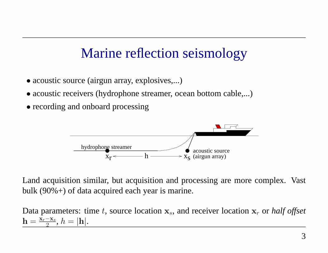
Marine reflection seismology

• acoustic source (airgun array, explosives,...)

• acoustic receivers (hydrophone streamer, ocean bottom cable,...)

• recording and onboard processing

hydrophone streameracoustic source(airgun array)x xr sh

Land acquisition similar, but acquisition and processing are more complex. Vastbulk (90%+) of data acquired each year is marine.

Data parameters: timet, source locationxs, and receiver locationxr or half offseth = xr−xs

2 , h = |h|.

3

Idealized marine “streamer” geometry:xs andxr lie roughly on constant depthplane, source-receiver lines are parallel→ 3 spatial degrees of freedom (eg.xs, h):codimension 1. [Other geometries are interesting, eg. ocean bottom cables, butstreamer surveys still prevalent.]

How much data? Contemporary surveys may feature

• Simultaneous recording by multiple streamers (up to 12!)

• Many (roughly) parallel ship tracks (“lines”), areal coverage

• single line (“2D”)∼ Gbyte; multiple lines (“3D”)∼ Tbyte

NB: In these lectures, will largely ignore sampling issues and treat data as contin-uously sampled.First of many approximations...

4

Gathers: distinguished data subsets

Aka “bins”, extracted from data after acquisition.

Characterized by common value of an acquisition parameter

• shot (or common source) gather: traces with same shot location xs (previousexpls)

• offset (or common offset) gather: traces with same half offset h

• ...

5

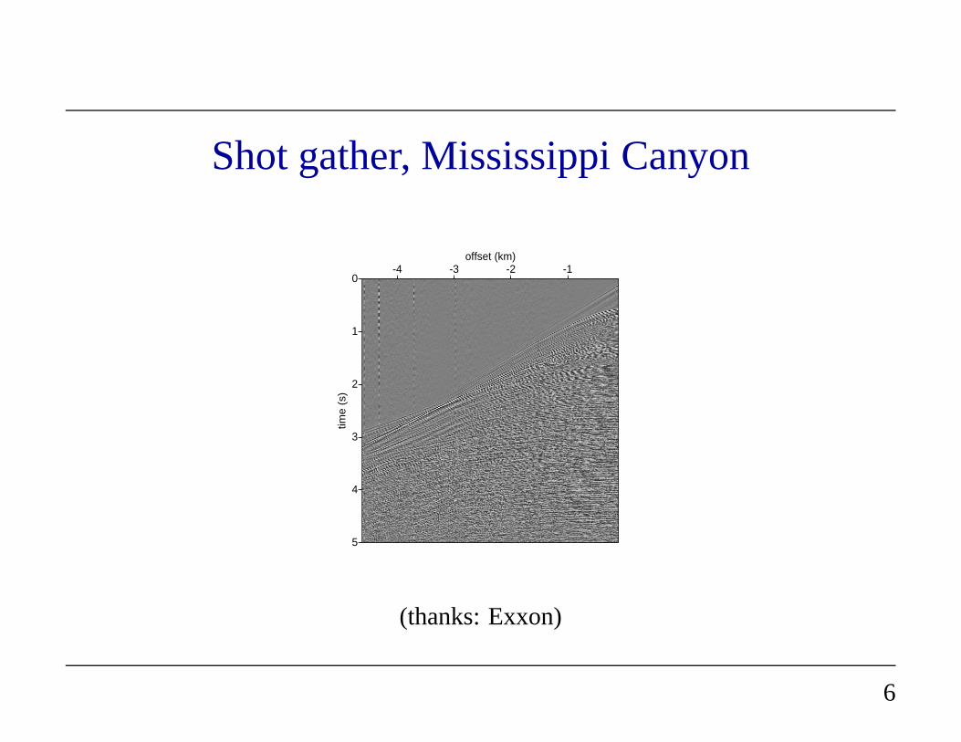
Shot gather, Mississippi Canyon

0

1

2

3

4

5

time

(s)

-4 -3 -2 -1offset (km)

(thanks: Exxon)

6

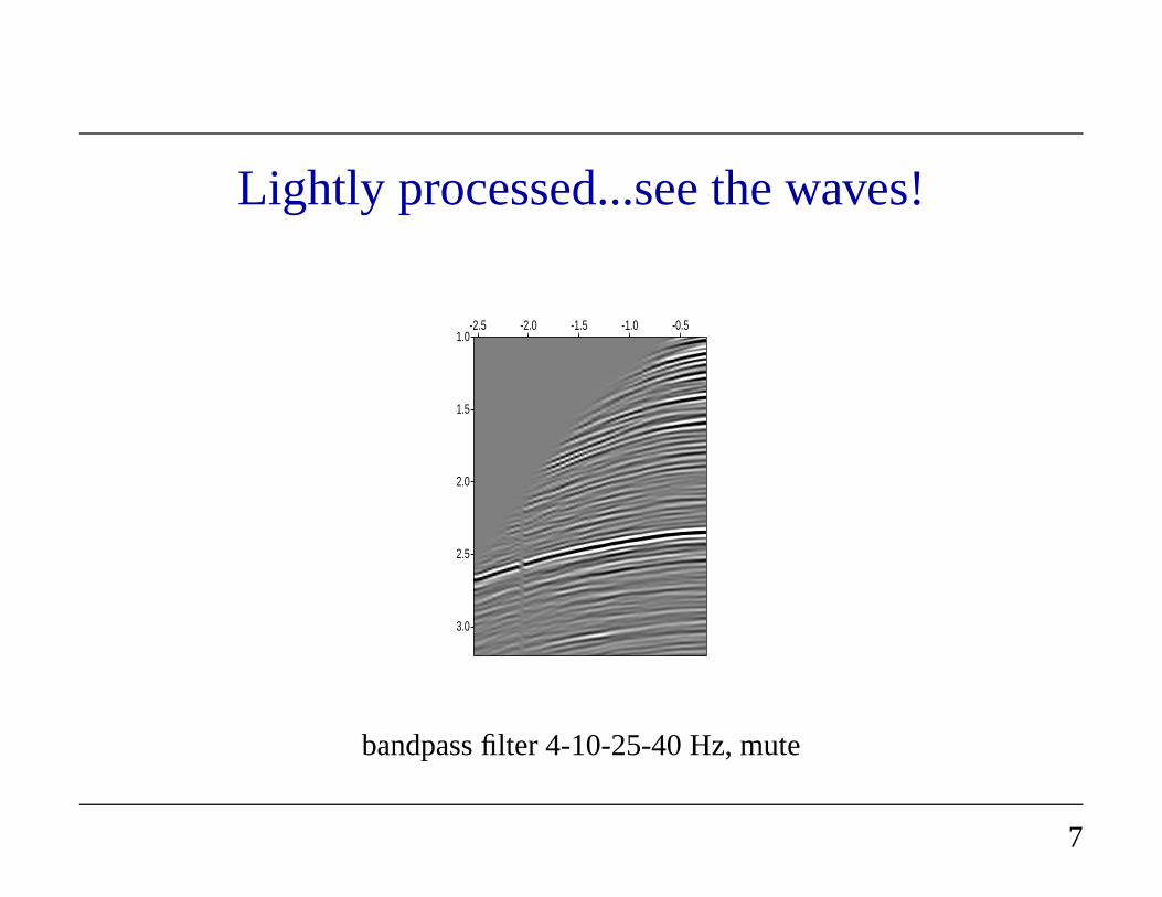
Lightly processed...see the waves!

1.0

1.5

2.0

2.5

3.0

-2.5 -2.0 -1.5 -1.0 -0.5

bandpass filter 4-10-25-40 Hz, mute

7

A key observation

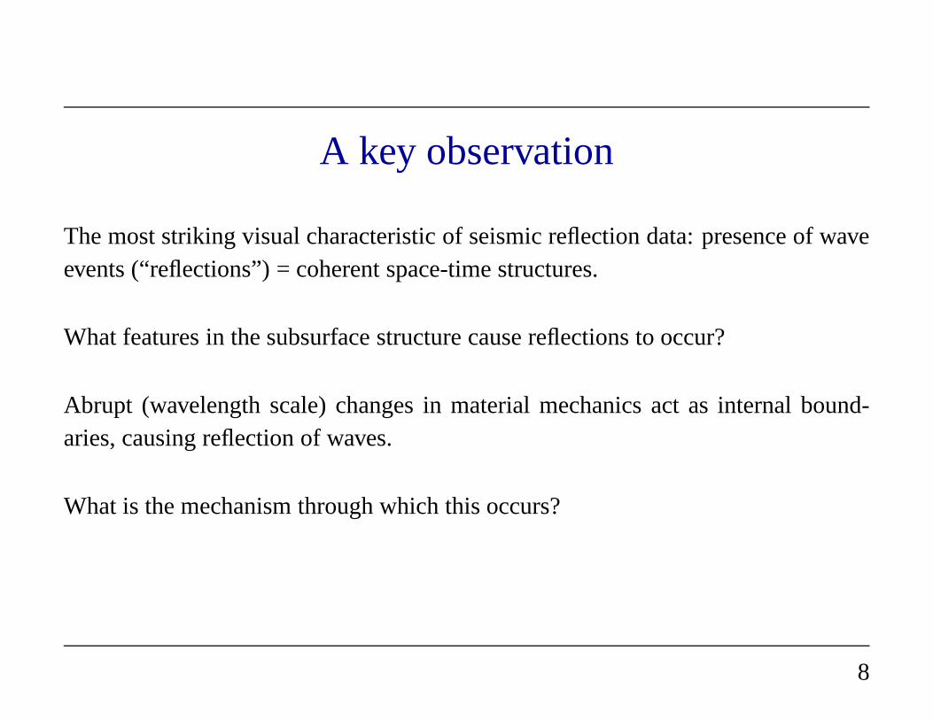
The most striking visual characteristic of seismic reflection data: presence of waveevents (“reflections”) = coherent space-time structures.

What features in the subsurface structure cause reflectionsto occur?

Abrupt (wavelength scale) changes in material mechanics act as internal bound-aries, causing reflection of waves.

What is the mechanism through which this occurs?

8

Well logs: a “direct” view of the subsurface

1000 1200 1400 1600 1800 2000 2200 2400 2600 2800 3000500

1000

1500

2000

2500

3000

3500

4000

4500

depth (m)

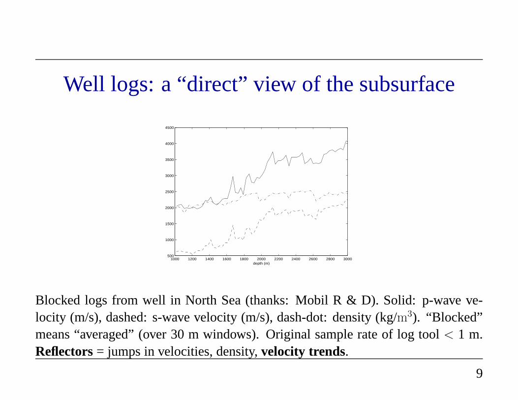
Blocked logs from well in North Sea (thanks: Mobil R & D). Solid: p-wave ve-locity (m/s), dashed: s-wave velocity (m/s), dash-dot: density (kg/m3). “Blocked”means “averaged” (over 30 m windows). Original sample rate of log tool < 1 m.Reflectors= jumps in velocities, density,velocity trends.

9

The Modeling Task

A useful model of the reflection seismology experiment must

• predict wave motion

• produce reflections from reflectors

• accomodate significant variation of wave velocity, material density,...

A really goodmodel will also accomodate

• multiple wave modes, speeds

• material anisotropy

• attenuation, frequency dispersion of waves

• complex source, receiver characteristics

10

The Acoustic Model

Not really good, but good enough for this week and basis of most contemporaryprocessing.

Relatesρ(x)= material density,λ(x) = bulk modulus,p(x, t)= pressure,v(x, t) =particle velocity,f(x, t)= force density (sound source):

ρ∂v

∂t= −∇p + f ,

∂p

∂t= −λ∇ · v (+ i.c.′s, b.c.′s)

(compressional) wave speedc =√

λρ

11

acoustic field potentialu(x, t) =∫ t

−∞ ds p(x, s):

p =∂u

∂t, v =

1

ρ∇u

Equivalent form: second order wave equation for potential

1

ρc2

∂2u

∂t2−∇ ·

1

ρ∇u =

∫ t

−∞

dt∇ ·

(

f

ρ

)

≡f

ρ

plus initial, boundary conditions.

12

Theory

Weak solutionof Dirichlet problem inΩ ⊂ R3 (similar treatment for other b. c.’s):

u ∈ C1([0, T ]; L2(Ω)) ∩ C0([0, T ]; H10(Ω))

satisfying for anyφ ∈ C∞0 ((0, T ) × Ω),

∫ T

0

∫

Ω

dt dx

1

ρc2

∂u

∂t

∂φ

∂t−

1

ρ∇u · ∇φ +

1

ρfφ

= 0

Theorem (Lions, 1972) Suppose thatlog ρ, log c ∈ L∞(Ω), f ∈ L2(Ω × R). Thenweak solutions of Dirichlet problem exist, uniquely determined by initial data

u(·, 0) ∈ H10(Ω),

∂u

∂t(·, 0) ∈ L2(Ω)

NB: No hint of waves here...

13

Further idealizations

• density is constant,

• source force density isisotropic point radiator with known time dependence(“source pulse”w(t))

f(x, t;xs) = w(t)δ(x− xs)

⇒ acoustic potential, pressure depends onxs also.

Forward map F [c] = time history of pressure for eachxs at receiver locationsxr

(predicted seismic data), as function of velocity fieldc(x):

F [c] = p(xr, t;xs)

14

Reflection seismic inverse problem

givenobserved seismic datad, find c so that

F [c] ≃ d

This inverse problem is

• large scale - up to Tbytes, Pflops

• nonlinear

• yields to no known direct attack

15

Partial linearization

Almost all useful technology to date relies on partial linearization: writec = v(1+r)

and treatr as relative first order perturbation aboutv, resulting in perturbation ofpresure fieldδp = ∂δu

∂t= 0, t ≤ 0, where

(

1

v2

∂2

∂t2−∇2

)

δu =2r

v2

∂2u

∂t2

Definelinearized forward map F by

F [v]r = δp(xr, t;xs)

Analysis ofF [v] is the main content of contemporary reflection seismic theory.

16

Linearization error

Critical question: If there is any justiceF [v]r = directional derivativeDF [v][vr]

of F - but in what sense? Physical intuition, numerical simulation, and not nearlyenough mathematics: linearization error

F [v(1 + r)] − (F [v] + F [v]r)

• smallwhenv smooth,r rough or oscillatory on wavelength scale - well-separatedscales

• largewhenv not smooth and/orr not oscillatory - poorly separated scales

2D finite difference simulation: shot gathers with typical marine seismic geometry.Smooth (linear)v(x, z), oscillatory (random)r(x, z) depending only onz(“layeredmedium”). Source waveletw(t) = bandpass filter.

17

0

0.2

0.4

0.6

0.8

1.0

z (k

m)

0 0.5 1.0 1.5 2.0x (km)

1.6

1.8

2.0

2.2

2.4

,

0

0.2

0.4

0.6

0.8

t (s)

0 0.2 0.4 0.6 0.8 1.0x_r (km)

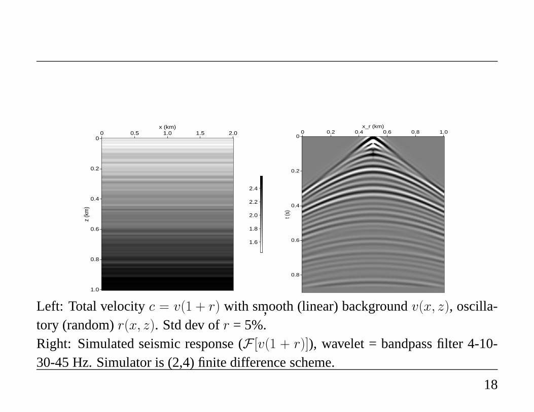
Left: Total velocityc = v(1 + r) with smooth (linear) backgroundv(x, z), oscilla-tory (random)r(x, z). Std dev ofr = 5%.Right: Simulated seismic response (F [v(1 + r)]), wavelet = bandpass filter 4-10-30-45 Hz. Simulator is (2,4) finite difference scheme.

18

0

0.2

0.4

0.6

0.8

1.0

z (k

m)

0 0.5 1.0 1.5 2.0x (km)

1.6

1.8

2.0

2.2

2.4

,

0

0.2

0.4

0.6

0.8

1.0z

(km

)

0 0.5 1.0 1.5 2.0x (km)

-0.10

-0.05

0

0.05

0.10

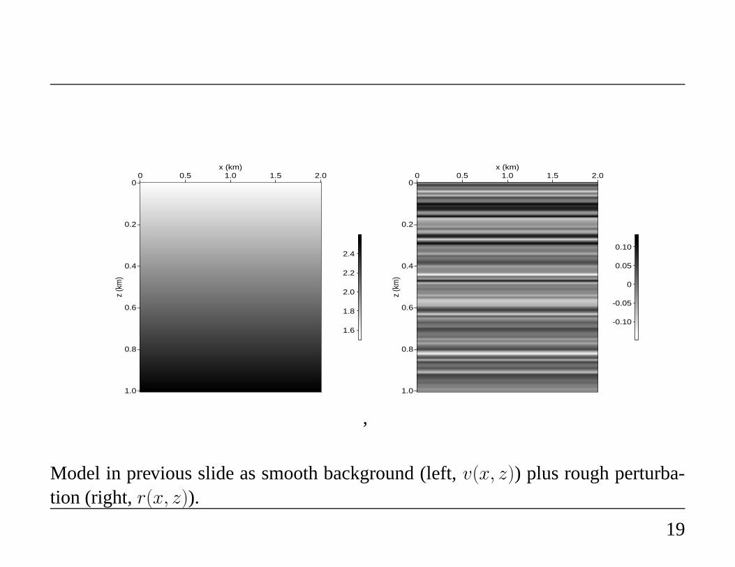
Model in previous slide as smooth background (left,v(x, z)) plus rough perturba-tion (right,r(x, z)).

19

0

0.2

0.4

0.6

0.8

t (s)

0 0.2 0.4 0.6 0.8 1.0x_r (km)

.

0

0.2

0.4

0.6

0.8

t (s)

0 0.2 0.4 0.6 0.8 1.0x_r (km)

Left: Simulated seismic response of smooth model (F [v]),Right: Simulated linearized response, rough perturbationof smooth model (F [v]r)

20

0

0.2

0.4

0.6

0.8

1.0

z (k

m)

0 0.5 1.0 1.5 2.0x (km)

1.4

1.6

1.8

2.0

2.2

2.4

,

Model in previous slide as rough background (left,v(x, z)) plus smooth 5% pertur-bation (r(x, z)).

21

0

0.2

0.4

0.6

0.8

t (s)

0 0.2 0.4 0.6 0.8 1.0x_r (km)

.

0

0.2

0.4

0.6

0.8

t (s)

0 0.2 0.4 0.6 0.8 1.0x_r (km)

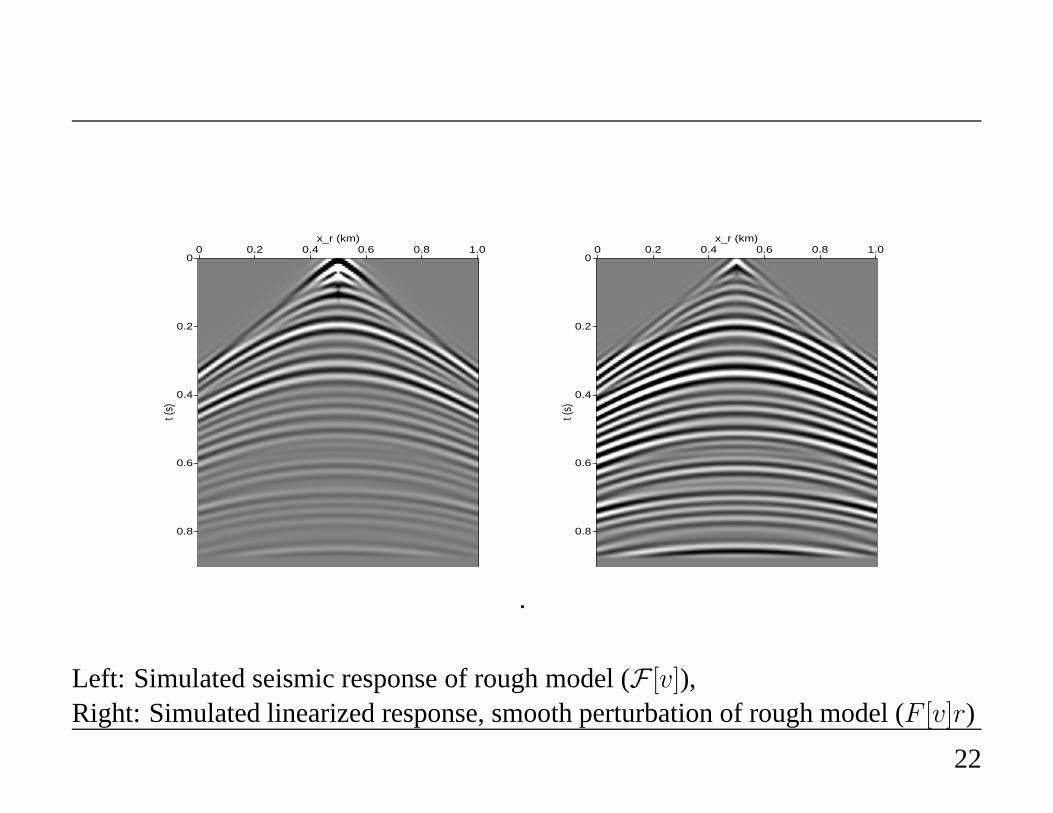
Left: Simulated seismic response of rough model (F [v]),Right: Simulated linearized response, smooth perturbation of rough model (F [v]r)

22

0

0.2

0.4

0.6

0.8

t (s)

0 0.2 0.4 0.6 0.8 1.0x_r (km)

,

0

0.2

0.4

0.6

0.8

t (s)

0 0.2 0.4 0.6 0.8 1.0x_r (km)

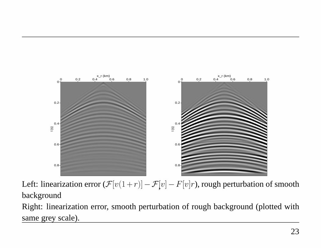
Left: linearization error (F [v(1+ r)]−F [v]−F [v]r), rough perturbation of smoothbackgroundRight: linearization error, smooth perturbation of rough background (plotted withsame grey scale).

23

Summary

• v smooth,r oscillatory⇒ F [v]r approximatesprimary reflection = result ofwave interacting with material heterogeneity only once (single scattering); errorconsists ofmultiple reflections, which are “not too large” ifr is “not too big”,and sometimes can be suppressed.

• v nonsmooth,r smooth⇒ error consists oftime shiftsin waves which are verylarge perturbations as waves are oscillatory.

No mathematical results are known which justify/explain these observations in anyrigorous way, except in 1D.

24

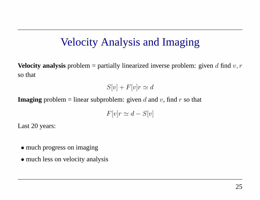
Velocity Analysis and Imaging

Velocity analysisproblem = partially linearized inverse problem: givend find v, r

so that

S[v] + F [v]r ≃ d

Imaging problem = linear subproblem: givend andv, find r so that

F [v]r ≃ d − S[v]

Last 20 years:

• much progress on imaging

• much less on velocity analysis

25

Aymptotic assumption

Linearization is accurate⇔ length scale ofv >> length scale ofr ≃ wavelength,properties ofF [v] dominated by those ofFδ[v] (= F [v] with w = δ). Implicit inmigration concept (eg. Hagedoorn, 1954); explicit use: Cohen & Bleistein, SIAMJAM 1977.

Key idea:reflectors (rapid changes inr) emulatesingularities; reflections(rapidlyoscillating features in data) also emulate singularities.

NB: “everybody’s favorite reflector”: the smooth interfaceacross whichr jumps.But this is an oversimplification - reflectors in the Earth may be complex zones ofrapid change, pehaps in all directions. More flexible notionneeded!!

26

Wave Front Sets

Recall characterization of smoothness via Fourier transform: u ∈ D′(Rn) is smoothatx0 ⇔ for some nbhdX of x0, anyφ ∈ E(X) andN , there isCN ≥ 0 so that foranyξ 6= 0,

∣

∣

∣

∣

F(φu)

(

τξ

|ξ|

)∣

∣

∣

∣

≤ CNτ−N

Harmonic analysis of singularities,apresHormander: thewave front setWF (u) ⊂R

n × Rn − 0 of u ∈ D′(Rn) - captures orientation as well as position of singu-

larities.

(x0, ξ0) /∈ WF (u) ⇔, there is some open nbhdX×Ξ ⊂ Rn×R

n−0 of (x0, ξ0)so that for anyφ ∈ E(X), N , there isCN ≥ 0 so that for allξ ∈ Ξ,

∣

∣

∣

∣

F(φu)

(

τξ

|ξ|

)∣

∣

∣

∣

≤ CNτ−N

27

Housekeeping chores

(i) note that the nbhdsΞ may naturally be taken to becones;

(ii) u is smooth atx0 ⇔ (x0, ξ0) /∈ WF (u) for all ξ0 ∈ Rn − 0;

(iii) WF (u) is invariant under chg. of coords if it is regarded as a subsetof thecotangent bundleT ∗(Rn) (i.e. theξ components transform as covectors).

[Good refs: Duistermaat, 1996; Taylor, 1981; Hormander, 1983]

The standard example: ifu jumps across the interfacef(x) = 0, otherwise smooth,thenWF (u) ⊂ Nf = (x, ξ) : f(x) = 0, ξ||∇f(x) (normal bundleof f = 0).

28

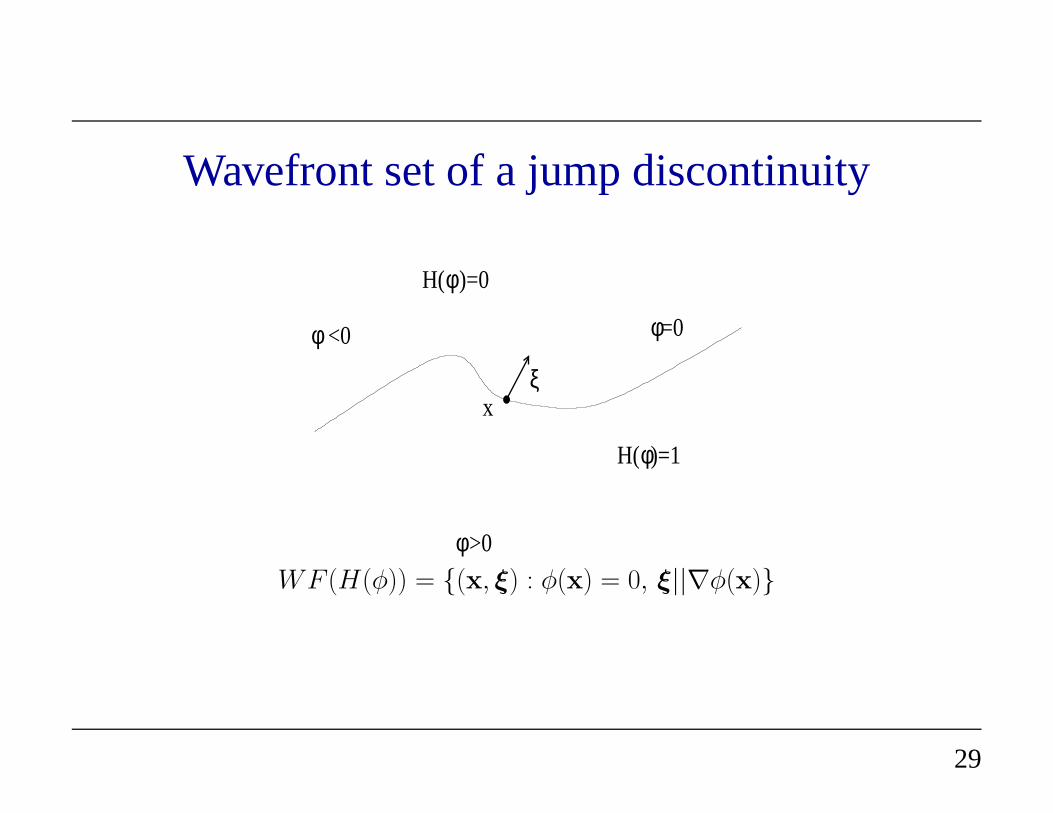
Wavefront set of a jump discontinuity

H(

)=0

φ

φ

=0φ

φ)=1

>0

<0

φH(

ξx

WF (H(φ)) = (x, ξ) : φ(x) = 0, ξ||∇φ(x)

29

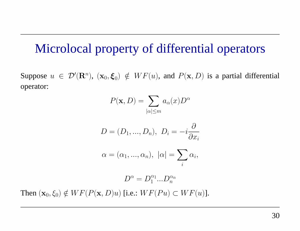
Microlocal property of differential operators

Supposeu ∈ D′(Rn), (x0, ξ0) /∈ WF (u), andP (x, D) is a partial differentialoperator:

P (x, D) =∑

|α|≤m

aα(x)Dα

D = (D1, ..., Dn), Di = −i∂

∂xi

α = (α1, ..., αn), |α| =∑

i

αi,

Dα = Dα11 ...Dαn

n

Then(x0, ξ0) /∈ WF (P (x, D)u) [i.e.: WF (Pu) ⊂ WF (u)].

30

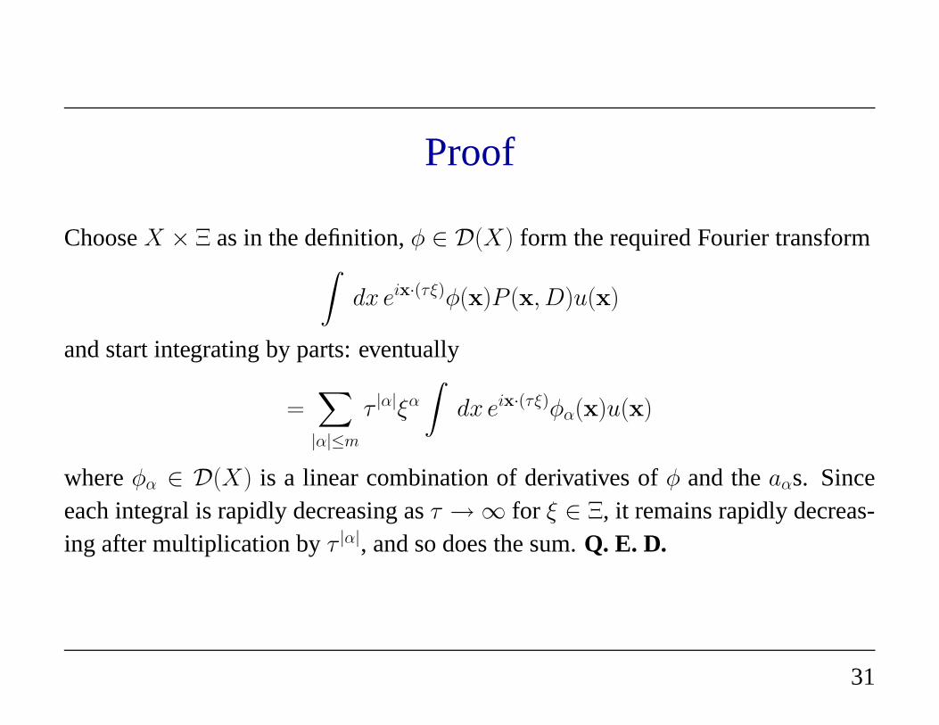
Proof

ChooseX × Ξ as in the definition,φ ∈ D(X) form the required Fourier transform∫

dx eix·(τξ)φ(x)P (x, D)u(x)

and start integrating by parts: eventually

=∑

|α|≤m

τ |α|ξα

∫

dx eix·(τξ)φα(x)u(x)

whereφα ∈ D(X) is a linear combination of derivatives ofφ and theaαs. Sinceeach integral is rapidly decreasing asτ → ∞ for ξ ∈ Ξ, it remains rapidly decreas-ing after multiplication byτ |α|, and so does the sum.Q. E. D.

31

Formalizing the reflector concept

Key idea, restated: reflectors (or “reflecting elements”) will be points inWF (r).Reflections will be points inWF (d).

These ideas lead to a usable definition ofimage: a reflectivity modelr is an imageof r if WF (r) ⊂ WF (r) (the closer to equality, the better the image).

Idealizedmigration problem : givend (henceWF (d)) deduce somehow a functionwhich hasthe right reflectors, i.e. a functionr with WF (r) ≃ WF (r).

NB: you’re going to needv! (“It all depends on v(x,y,z)” - J. Claerbout)

32

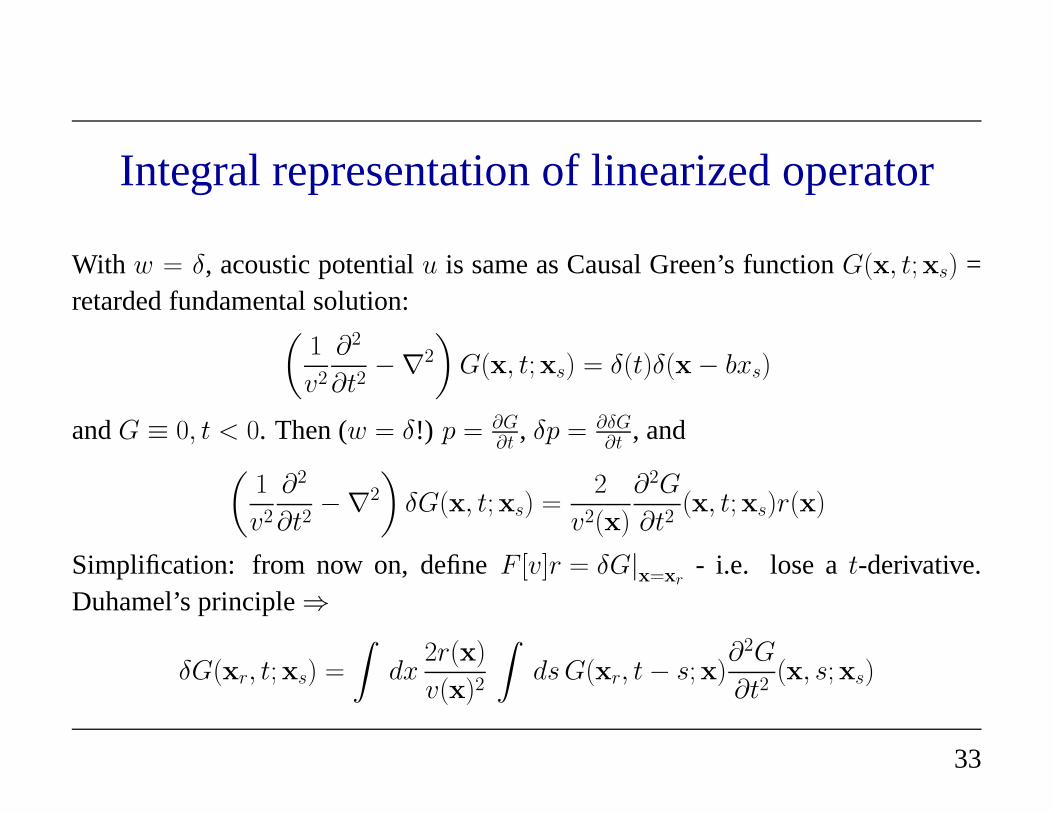
Integral representation of linearized operator

With w = δ, acoustic potentialu is same as Causal Green’s functionG(x, t;xs) =retarded fundamental solution:

(

1

v2

∂2

∂t2−∇2

)

G(x, t;xs) = δ(t)δ(x − bxs)

andG ≡ 0, t < 0. Then (w = δ!) p = ∂G∂t , δp = ∂δG

∂t , and(

1

v2

∂2

∂t2−∇2

)

δG(x, t;xs) =2

v2(x)

∂2G

∂t2(x, t;xs)r(x)

Simplification: from now on, defineF [v]r = δG|x=xr

- i.e. lose at-derivative.Duhamel’s principle⇒

δG(xr, t;xs) =

∫

dx2r(x)

v(x)2

∫

dsG(xr, t − s;x)∂2G

∂t2(x, s;xs)

33

Add geometric optics...

Geometric optics approximation ofG should be good, asv is smooth. Summary: ifx “not too far” fromxs, then

G(x, t;xs) = a(x;xs)δ(t − τ (x; xs)) + R(x, t;xs)

where the traveltimeτ (x; xs) solves the eikonal equation

v|∇τ | = 1, τ (x;xs) ∼|x − xs|

v(xs), x → xs

and the amplitudea(x;xs) solves the transport equation

∇ · (a2∇τ ) = 0, ...

Refs: Courant & Hilbert, FriedlanderSound Pulses, WWSFoundationsand manyrefs cited there...

34

Simple Geometric Optics

“Not too far” means: there should be one and only one ray of geometric opticsconnecting eachxs or xr to eachx ∈ suppr.

Will call this thesimple geometric opticsassumption.

Within region satisfying simple geometric optics assumption,τ is smooth (x 6= xs)solution of eikonal equation. Effective methods for numerical solution of eikonal,transport equations: ray tracing (Lagrangian), various sorts of upwind finite differ-ence (Eulerian) methods. See eg. Sethian book, WWS 1999 MGSSnotes (online)for details.

35

Caution - caustics!

For “random but smooth”v(x) with varianceσ, more than one connecting ray oc-curs as soon as the distance isO(σ−2/3). Suchmultipathingis invariably accompa-nied by the formation of acaustic= envelope of rays (White, 1982).

Upon caustic formation, the simple geometric optics field description above is nolonger correct.

Failure of GO at caustic understood in 19th century. Generalization of GO to re-gions containing caustics accomplished by Ludwig and Kravtsov, 1966-7, elabo-rated by Maslov, Hormander, Duistermaat, many others.

36

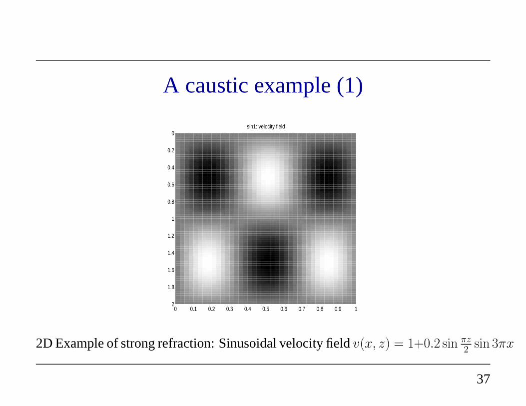
A caustic example (1)

0 0.1 0.2 0.3 0.4 0.5 0.6 0.7 0.8 0.9 1

0

0.2

0.4

0.6

0.8

1

1.2

1.4

1.6

1.8

2

sin1: velocity field

2D Example of strong refraction: Sinusoidal velocity fieldv(x, z) = 1+0.2 sin πz2

sin 3πx

37

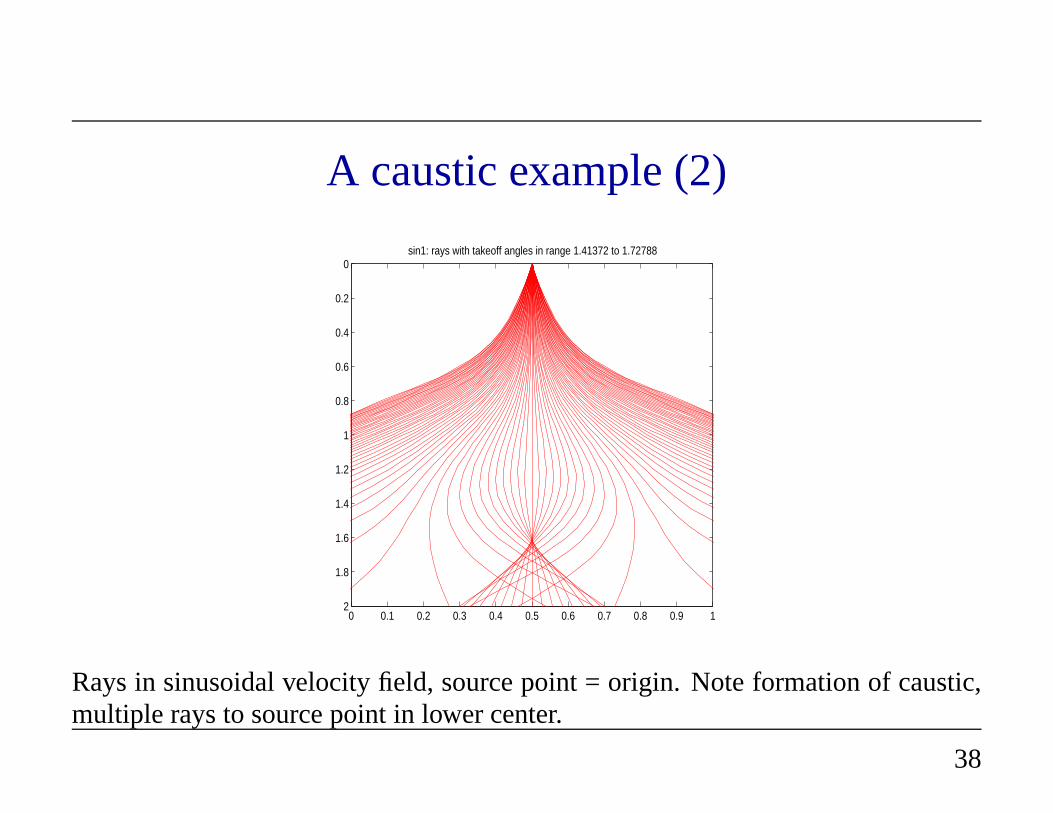
A caustic example (2)

0 0.1 0.2 0.3 0.4 0.5 0.6 0.7 0.8 0.9 1

0

0.2

0.4

0.6

0.8

1

1.2

1.4

1.6

1.8

2

sin1: rays with takeoff angles in range 1.41372 to 1.72788

Rays in sinusoidal velocity field, source point = origin. Note formation of caustic,multiple rays to source point in lower center.

38

An oft-forgotten detail

All of this is meaningful only if the remainderR is small in a suitable sense: energyestimate (Exercise!) ⇒

∫

dx

∫ T

0

dt |R(x, t;xs)|2 ≤ C‖v‖C4

(this is an easy, suboptimal estimate - with more work can replace 4 with 2)

If v ∈ C∞, can complete the geometric optics approximation of the Green’s func-tion so that the difference isC∞ - then the two sides have the same singularities, ie.the same wavefront set.

39

Finally, a wave!

The geometric optics approximation to the Green’s function

G(x, t;xs) ≃ a(x;xs)δ(t − τ (x; xs))

describes a (singular) quasi-spherical waves [spherical,if v = const., for thenτ (x,xs) = |x − xs|/v].

Geometric optics is the the best currently available explanation for waves in het-erogeneous media.Note the inadequacy:v must besmooth, but the compressionalvelocity distribution in the Earth varies on all scales!

40

The linearized operator as Generalized Radon

Transform

Assume:supp r contained in simple geometric optics domain (each point reachedby unique ray from any source or receiver point).

Then distribution kernelK of F [v] is

K(xr, t,xs;x) =

∫

dsG(xr, t − s;x)∂2G

∂t2(x, s;xs)

2

v2(x)

≃

∫

ds2a(xr,x)a(x,xs)

v2(x)δ′(t − s − τ (xr,x))δ′′(s − τ (x,xs))

41

=2a(x,xr)a(x,xs)

v2(x)δ′′(t − τ (x,xr) − τ (x,xs))

provided that

∇xτ (x,xr) + ∇xτ (x,xs) 6= 0

⇔ velocity atx of ray fromxs not negative of velocity of ray fromxr ⇔ no forwardscattering. [Gel’fand and Shilov, 1958 - when is pullback of distribution again adistribution].

42

GRT = “Kirchhoff” modeling

So: forr supported in simple geometric optics domain, no forward scattering⇒

δG(xr, t;xs) ≃

∂2

∂t2

∫

dx2r(x)

v2(x)a(x,xr)a(x,xs)δ(t − τ (x,xr) − τ (x,xs))

That is: pressure perturbation is sum (integral) ofr over reflection isochronx :

t = τ (x,xr) + τ (x,xs), w. weighting, filtering. Note: ifv =const. then isochronis ellipsoid, asτ (xs,x) = |xs − x|/v!

(y,x )+ (y,x )ττt=

x x

y

s

r s

r

43

Zero Offset data and the Exploding Reflector

Zero offset data (xs = xr) is seldom actually measured (contrast radar, sonar!), butroutinelyapproximatedthroughNMO-stack(to be explained later).

Extracting image from zero offset data, rather than from all(100’s) of offsets, istremendousdata reduction- when approximation is accurate, leads to excellentimages.

Imaging basis: theexploding reflectormodel (Claerbout, 1970’s).

44

For zero-offset data, distribution kernel ofF [v] is

K(xs, t,xs;x) =∂2

∂t2

∫

ds2

v2(x)G(xs, t − s;x)G(x, s;xs)

Under some circumstances (explained below),K ( = G time-convolved with itself)is “similar” (also explained) toG = Green’s function forv/2. Then

δG(xs, t;xs) ∼∂2

∂t2

∫

dx G(xs, t,x)2r(x)

v2(x)

∼ solutionw of(

4

v2

∂2

∂t2−∇2

)

w = δ(t)2r

v2

Thus reflector “explodes” at time zero, resulting field propagates in “material” withvelocity v/2.

45

Explain when the exploding reflector model “works”, i.e. when G time-convolvedwith itself is “similar” to G = Green’s function forv/2. If supp r lies in simplegeometry domain, then

K(xs, t,xs;x) =

∫

ds2a2(x,xs)

v2(x)δ(t − s − τ (xs,x))δ′′(s − τ (x,xs))

=2a2(x,xs)

v2(x)δ′′(t − 2τ (x,xs))

whereas the Green’s functionG for v/2 is

G(x, t;xs) = a(x,xs)δ(t − 2τ (x,xs))

(half velocity = double traveltime, same rays!).

46

Difference between effects ofK, G: for eachxs scaler by smooth fcn - preservesWF (r) henceWF (F [v]r) and relation between them. Also: adjoints have sameeffect onWF sets.

Upshot: from imaging point of view (i.e. apart from amplitude, derivative (filter)),kernel ofF [v] restricted to zero offset is same as Green’s function forv/2, providedthat simple geometry hypothesis holds:only one ray connects each source point toeach scattering point, ie.no multipathing.

See Claerbout, IEI, for examples which demonstrate that multipathing really doesinvalidate exploding reflector model.

47

Standard Processing

Inspirational interlude: the sort-of-layered theory =“Standard Processing”

Suppose werev,r functions ofz = x3 only, all sources and receivers atz = 0.Then the entire system is translation-invariant inx1, x2 ⇒ Green’s functionG itsperturbationδG, and the idealized dataδG|z=0 are really only functions oft, z, andhalf-offseth = |xs−xr|/2. There would beonly one seismic experiment, equivalentto anycommon midpoint gather(“CMP”).

This isn’t really true -look at the data!!! However it isapproximatelycorrect inmany places in the world: CMPs change very slowly with midpoint xm = (xr +

xs)/2.

48

Standard processing: treat each CMPas if it were the result of an experiment per-formed over a layered medium, but permit the layers to vary with midpoint.

Thusv = v(z), r = r(z) for purposes of analysis, but at the endv = v(xm, z), r =

r(xm, z).

F [v]r(xr, t;xs)

≃

∫

dx2r(z)

v2(z)a(x, xr)a(x, xs)δ

′′(t − τ (x, xr) − τ (x, xs))

=

∫

dz2r(z)

v2(z)

∫

dω

∫

dxω2a(x, xr)a(x, xs)eiω(t−τ(x,xr)−τ(x,xs))

49

Since we have already thrown away smoother (lower frequency) terms, do it againusingstationary phase.Upshot (see 2000 MGSS notes for details): up to smoother(lower frequency) error,

F [v]r(h, t) ≃ A(z(h, t), h)R(z(h, t))

Herez(h, t) is the inverse of the 2-way traveltime

t(h, z) = 2τ ((h, 0, z), (0, 0, 0))

i.e. z(t(h, z′), h) = z′. R is (yet another version of) “reflectivity”

R(z) =1

2

dr

dz(z)

That is,F [v] is a a derivative followed by a change of variable followed bymulti-plication by a smooth function. Substitutet0 (vertical travel time) forz (depth) andyou get “Inverse NMO” (t0 → (t, h)). Will be sloppy and callz → (t, h) INMO.

50

Anatomy of an adjoint

∫

dt

∫

dh d(t, h)F [v]r(t, h) =

∫

dt

∫

dh d(t, h)A(z(t, h), h)R(z(t, h))

=

∫

dz R(z)

∫

dh∂t

∂z(z, h)A(z, h)d(t(z, h), h) =

∫

dz r(z)(F [v]∗d)(z)

soF [v]∗ = − ∂∂z

SM [v]N [v], where

• N [v] = NMO operator N [v]d(z, h) = d(t(z, h), h)

• M [v] = multiplication by ∂t∂z

A

• S = stacking operatorSf(z) =∫

dh f(z, h)

51

Normal Op is PDO⇒ Imaging

F [v]∗F [v]r(z) = −∂

∂z

[∫

dhdt

dz(z, h)A2(z, h)

]

∂

∂zr(z)

Microlocal property of PDOs⇒ WF (F [v]∗F [v]r) ⊂ WF (r) i.e. F [v]∗ is an imag-ing operator.

If you leave out the amplitude factor (M [v]) and the derivatives, as is commonlydone, then you get essentially the same expression - so (NMO,stack) is an imagingoperator!

It’s even easy to get an (asymptotic) inverse out of this - exercise for the reader.

Now make everything dependent onxm and you’ve got standard processing. (endof layered interlude).

52

But the Earth is not layered!

In general,

Is F [v]∗ an imaging operator?

What sort of thing isF [v]∗F [v]??

Stay tuned!

53