Pilot Models for Estimating Bicycle Intersection Volumes

UC BerkeleyResearch Reports

TitlePilot Models for Estimating Bicycle Intersection Volumes

Permalinkhttps://escholarship.org/uc/item/380855q6

AuthorsGriswold, Julia B.Medury, AdityaSchneider, Robert J.

Publication Date2011 Peer reviewed

eScholarship.org Powered by the California Digital LibraryUniversity of California

https://escholarship.org/uc/item/380855q6

https://escholarship.org

http://www.cdlib.org/

Pilot Models for Estimating Bicycle Intersection Volumes

Julia B. Griswold, SafeTREC, Aditya Medury, Institute of Transportation Studies, Berkeley, and

Robert J. Schneider, SafeTREC

2011RR-2011-2 http://www.safetrec.berkeley.edu

Pilot Models for Estimating Bicycle Intersection Volumes 1 2

3

Julia B. Griswold (Corresponding Author) 4

Safe Transportation Research and Education Center 5

University of California, Berkeley 6

2614 Dwight Way #7374 7

Berkeley, CA 94720, U.S.A 8

Telephone: (510) 643-0566 9

Fax: (510) 643-9922 10

Email: [email protected] 11

12

Aditya Medury 13

Department of Civil and Environmental Engineering 14

Institute of Transportation Studies 15



18

Robert J. Schneider 19

Safe Transportation Research and Education Center 20


2614 Dwight Way #7374 22

Berkeley, CA 94720 23

Telephone: (510) 643-0566 24

Fax: (510) 643-9922 25


27

28

29

30

31

32

33

34

35

36

37

38

39

40

41

42

43

44

45

46

47

Word Count: 5,030 + (4 tables + 1 figure) × 250 = 6,280 words 48

49

Submitted to the Transportation Research Board 90th Annual Meeting 50

TRB 2011 Annual Meeting Paper revised from original submittal.

Griswold, Medury, and Schneider 2

Pilot Models for Estimating Bicycle Intersection Volumes 1

2

ABSTRACT 3 Bicycle volume data are useful to practitioners and researchers to understand safety, travel behavior, and 4

development impacts. This paper describes the methodology used to develop several simple models of 5

bicycle intersection volumes in Alameda County, California. The models are based on two-hour bicycle 6

counts performed at a sample of 81 intersections in the Spring of 2008 and 2009. Study sites represented 7

areas with a wide range of population density, employment density, proximity to commercial property, 8

neighborhood income, and street network characteristics. The explanatory variables considered for the 9

models included intersection site, land use, transportation system, and socioeconomic characteristics of 10

the areas surrounding each intersection. Four alternative models are presented with adjusted R-square 11

values ranging from 0.39 to 0.60. The models showed that bicycle volumes tended to be higher at 12

intersections surrounded by more commercial retail properties within 1/10 mile, closer to a major 13

university, with a marked bicycle facility on at least one leg of the intersection, surrounded by less hilly 14

terrain within 1/2 mile, and surrounded by a more connected roadway network. The models also showed 15

several important differences between weekday and weekend intersection volumes. The positive 16

association between bicycle volume and proximity to retail or a large university was greater on weekdays 17

than weekends, while bicycle facilities had a stronger positive association and hilly terrain had a weaker 18

negative association with bicycle volume on weekends than weekdays. Further testing and refinement is 19

necessary before accurate count predictions can be made in Alameda County or other communities. 20

21

22

23



Bicycling is increasing in many United States communities. Nationwide, the proportion of commuters 1

traveling to work regularly by bicycle grew from 0.45% to 0.55% between 2006 and 2008 (1,2). Cities 2

such as Portland, New York, Seattle, and San Francisco documented increases in bicycle counts over this 3

same time period (3,4,5,6). Bicycling is a convenient and economical mode for commuting, small 4

shopping trips, transit access, and recreation. Estimates of bicycle activity are valuable to planners, 5

engineers, designers, public health professions, and others. However, there are very few tools available to 6

estimate the number of bicyclists that pass by specific locations or use particular intersections within an 7

urban area. A predictive model of bicycle volumes can be used to: 8

Quantify bicycle exposure in safety analyses, providing the denominator in the calculation of 9

crash risk; 10

Identify priority locations for bicycle facility improvements or safety measures; and 11

Estimate changes in bicycle volumes that will occur with new developments, roadway changes, 12

or new transit projects. 13

14

STUDY PURPOSE 15 The purpose of this study is to present several preliminary models that can be used to estimate bicycle 16

intersection volumes. A simple model structure, loglinear regression, was chosen so that the models 17

would be easy to apply using geographic information systems (GIS) and simple spreadsheet software. 18

Since the analysis was conducted in one urban area (Alameda County, California), more research is 19

needed to refine the model equations and determine the applicability of the results for other communities. 20

These models are designed for planning purposes to help identify built environment characteristics 21

associated with higher and lower levels of bicycling and show general differences in bicycle volumes at 22

intersections throughout a city or region. Applications that require precise bicycle volume data for 23

individual intersections should use actual bicycle counts from each location. 24

25

PREVIOUS STUDIES 26 Several techniques have been developed to analyze bicycle activity in different locations. Overlay 27

mapping techniques, or sketch-plan methods, are useful for planning and prioritization (7,8,9). However, 28

they are not typically calibrated to actual bicycle counts. Most previous efforts to model bicycle activity 29

have used zonal areas or the individual as the unit of analysis. Some regional travel demand models have 30

been adjusted to estimate bicycle mode share within a certain area (10), but these models are usually 31

estimated at the traffic analysis zone (TAZ) level and are not fine-grained enough to capture intersection-32

level bicycle activity. Models that examine behavior at the level of the individual are valuable for 33

identifying factors that determine mode and route choice, but they are difficult to use for volume 34

estimates. Most of these models are based on detailed household travel survey data, which can be 35

expensive to collect. 36

Two recent studies in Southern California have developed predictive models of bicycle volume, 37

using linear regression with bicycle counts as the dependent variable and demographic and land use 38

measures for the independent variables. Four land use and transportation system explanatory variables 39

(afternoon bus frequency, land use mix, density of residents under age 18, and proximity to the bicycle 40

network) were used to predict weekday afternoon peak hour bicycle volumes at intersections in the City 41

of Santa Monica (11). However, the ordinary least squares regression equation used for the model could 42

produce negative predictions. This modeling issue was addressed in San Diego County by using the 43

natural logarithm of the dependent variable, but the San Diego model was limited to two explanatory 44

variables (employment density and length of nearby multi-use trails) for predicting weekday 7 a.m. to 9 45

a.m. bicycle volumes (12). 46

An additional bicycle modeling study explored applying Space Syntax measures in a bicycle 47

model. A Space Syntax measure representing direct paths in the street network was combined with land 48

use variables to predict morning peak hour bicycle volumes at intersections and street segments in 49

Cambridge, MA (13). The model performed fairly well, but the sample size was small (n=16) and the 50



land use variables (population and employment density) explained most of the variation in the bicycle 1

volumes. In addition, the Space Syntax measure required special software to calculate. 2

Table 1 summarizes the factors that have been associated with bicycle activity in these modeling 3

efforts and other bicycle studies. 4

5

Table 1. Factors Associated with Bicycling in Previous Research 6

Variable

Relationship with

Bicycle Activity Source

Environmental and Land Use Variables

Nearby population density + McCahill and Garrick (2008) (13)

Nearby employment density + McCahill and Garrick (2008) (13), Jones et al.

(2010) (12)

Land use mix + Haynes and Andrzejewski (2010) (12)

Proximity to downtown + Dill and Voros (2007) (14)

Slope - Aultman-Hall, Hall, and Baetz (1997) (15), Dill

and Gliebe (2008) (16)

Transportation System Variables

Nearby street connectivity + Dill and Voros (2007) (14)

Proximity to a freeway + Dill and Voros (2007) (14)

Amount of bicycle lanes nearby + Dill and Carr (2003) (17)

Amount of multi-use trails nearby + Jones et al. (2010) (12)

Presence of bicycle facility + Dill and Gliebe (2008) (16), Stinson and Bhat

(2003) (18)

Proximity to bicycle network + Haynes and Andrzejewski (2010) (12)

Afternoon peak hour bus frequency + Haynes and Andrzejewski (2010) (12)

Motor vehicle volume - Stinson and Bhat (2003) (18)

Major arterial - Stinson and Bhat (2003) (18)

Parallel parking permitted - Stinson and Bhat (2003) (18)

Smooth pavement + Stinson and Bhat (2003) (18)

Socioeconomic Variables

Age 18-55 + Dill and Voros (2007) (14)

Age - Xing, Handy, and Buehler (2008) (19)

% of nearby population under age 18 - Haynes and Andrzejewski (2010) (12)

Education level + Xing, Handy, and Buehler (2008) (19)

Income + Dill and Voros (2007) (14)

Household automobile availability - Dill and Voros (2007) (14), Dill and Carr (2003)

(17)

7

8

METHODOLOGY 9 This section describes the study area, the bicycle count collection, and the development of the explanatory 10

variables. The model is based on bicycle counts taken at 81 intersections along arterial and collector 11

streets in Alameda County, California (Figure 1). 12

13



1 Figure 1. Map of Manual Bicycle Count Locations 2

3

Study Area 4 Alameda County is located on the eastern side of the San Francisco Bay across the Bay Bridge from San 5

Francisco, and it stretches east and south towards the San Joaquin Valley. Its population in 2008 was 6

estimated to be 1.47 million (2). The western portion of the county was largely developed in the early to 7

mid-twentieth century and contains several small downtown commercial areas and many streetcar suburbs 8

with grid street patterns. The hill areas and the eastern portion of the county were mostly developed in 9

the second half of the twentieth century; these areas are more suburban in nature, with curvilinear street 10

patterns. The largest city in the county is Oakland, with an estimated population of approximately 11

366,000 (2). In 2008, estimates are that 48 percent of the county population was white, 25 percent Asian, 12

22 percent Hispanic or Latino, and 13 percent black (2). 13

14

Bicycle Counts 15 The bicycle counts for this study were collected in the spring of 2008 and 2009 in conjunction with a 16

study of pedestrian exposure and crash risk. While the pedestrian study determined that the counts would 17

be at intersections, the count locations were also appropriate for understanding bicycle exposure because 18

approximately half of bicycle crashes occur at intersections (20). Counts were taken at 50 intersections in 19

2008 and 31 in 2009. All intersections were along arterial or collector roadways. A strategic process was 20

used to select intersections, ensuring that the set of study sites represented areas with a wide range of 21

population density, employment density, proximity to commercial properties, neighborhood incomes, and 22

other socioeconomic characteristics. In addition, the study intersections had a variety of roadway 23

characteristics. Of the 81 intersections, 16 (20%) had a marked bicycle facility (e.g., bicycle lane, bicycle 24



boulevard, or shared lane marking) on at least one approach. The choice of intersection locations is 1

described in detail in Schneider, Arnold, and Ragland (21) and Schneider et al. (22). 2

Each bicycle was logged according to the movement that was made at the intersection—straight, 3

right turn, or left turn from one of the four intersection legs—which made a total of 12 possible 4

movements. Bicycles being ridden either on the street or on the sidewalk were included, but bicycles 5

being walked were logged as pedestrians. The counts for each movement were summed together to find 6

the total bicycle volume for the intersection. Counts were conducted for two 2-hour periods at each 7

intersection. One was taken on a Tuesday, Wednesday, or Thursday, and one was taken on a Saturday. 8

The time of day for the counts varied depending on data collector scheduling. Counts were taken during 9

12 p.m.-2 p.m., 2 p.m.-4 p.m., 3 p.m.-5 p.m., or 4 p.m-6 p.m. on weekdays and 9 a.m.-11 a.m., 12 p.m.-2 10

p.m., 3 p.m.-5 p.m., or 4 p.m-6 p.m. on weekends. Additional information about the count methodology 11

is provided in Schneider, Arnold, and Ragland (21) and Schneider et al. (22). Table 2 includes summary 12

statistics for the bicycle count data. 13

14

Table 2. Summary Statistics for all Two-Hour Bicycle Counts 15

Statistic All Counts Weekday Weekend

Number of Counts 162 81 81

Minimum 0 0 1

Maximum 343 343 171

Median 23.5 22 24

Mean 35.8 38.6 33.0

Standard Deviation 41.4 50.3 30.1

16

ANALYSIS 17 The data analysis process for the model estimation included three steps: (a) explanatory variables were 18

screened to eliminate those weakly correlated to the dependent variable; (b) the remaining variables were 19

screened for collinearity to avoid including strongly correlated variables in the same model; and (c) four 20

alternative model structures were chosen for strong goodness-of-fit and significant coefficients. 21

22

Regression Modeling 23 Loglinear ordinary least squares (OLS) regression was used to estimate a model of bicycle intersection 24

volume. In loglinear regression, the dependent variable is transformed using the natural logarithm. This 25

is an appropriate method for modeling count data because when the natural log predictions are 26

transformed back to counts using the exponential, there are no negative values. A negative binomial form 27

of the regression model was also tested during the analysis process, and the model coefficients were 28

similar. The loglinear form was selected because it is easy to apply using spreadsheet software and 29

because it is easier to interpret the model goodness-of-fit and independent variable coefficients. One 30

intersection had a count of zero bicyclists. This count was changed to 0.1 to allow the log to be 31

computed. The model formulation is: 32

33

(1) 34

35

where: 36

Yi = bicycle counts at intersection i 37

Xji = value of explanatory variable j at intersection i 38

βj = model coefficient for variable j 39

40

The modeling process examined the relationship between the bicycle intersection volume and the 41

built environment surrounding the intersection, such as nearby land use, transportation system, and site 42

characteristics. Some of the measures were evaluated at different scales, including buffer radii of 0.1 mi 43



(161 m), 0.25 mi (402 m), and 0.5 mi (805 m). This study took advantage of explanatory variables 1

previously developed for the 81 intersections for pedestrian volume and pedestrian crash models (21,22). 2

Several additional factors used in previous studies were also included, bringing the total to more than 70 3

variables considered in the analysis. Network distance to UC Berkeley Campus and Oakland City Center 4

were included to account for two of the major trip attractors in the county. Connected node ratio was 5

calculated using GIS. This measure represented the ratio of three- and four-way intersections to dead-end 6

streets in the area around each study intersection. Areas with lower connected node ratios had higher 7

proportions of dead ends. The new variables and any existing variables that were used in the final 8

bicycle volume models are described in Table 3. Descriptions of the other variables considered for the 9

analysis can be found in Schneider, Arnold, and Ragland (21) and Schneider et al. (22). 10

It was necessary to narrow down the number of independent variables to avoid overfitting the 11

model. Models with nearly as many independent variables as the number of observations they are based 12

on predict volumes poorly. First, correlation coefficients were estimated between each explanatory 13

variable and the bicycle counts. Those variables with weak correlation (ρ < 0.2) were eliminated from the 14

analysis. Next, the remaining independent variables were screened for collinearity; pairs of variables with 15

moderate to strong correlation (ρ > 0.3) were not included in the same model. 16

17

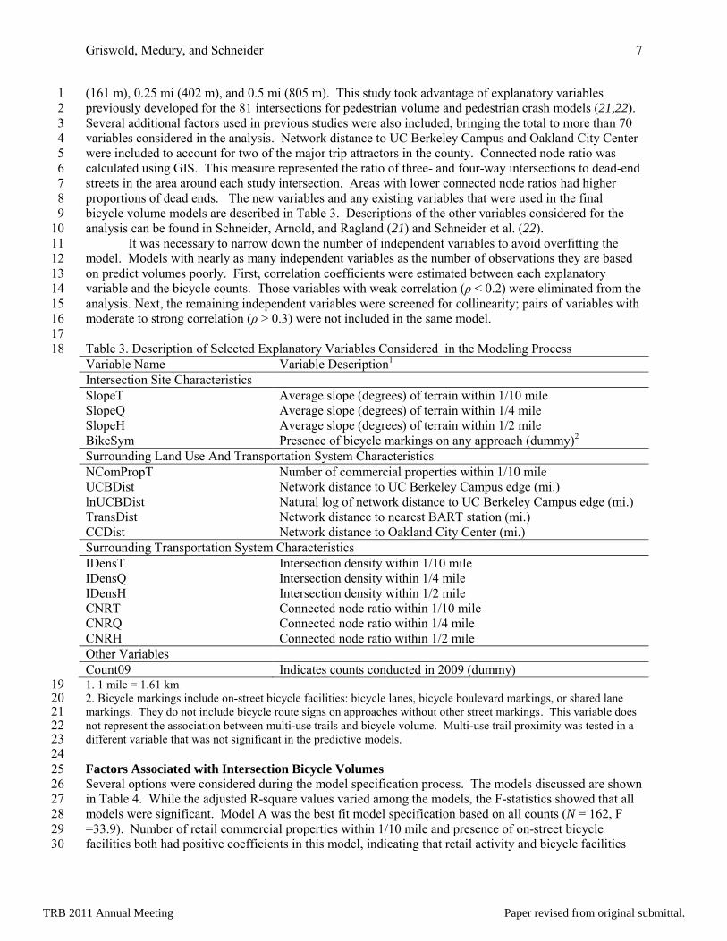
Table 3. Description of Selected Explanatory Variables Considered in the Modeling Process 18

Variable Name Variable Description1

Intersection Site Characteristics

SlopeT Average slope (degrees) of terrain within 1/10 mile

SlopeQ Average slope (degrees) of terrain within 1/4 mile

SlopeH Average slope (degrees) of terrain within 1/2 mile

BikeSym Presence of bicycle markings on any approach (dummy)2

Surrounding Land Use And Transportation System Characteristics

NComPropT Number of commercial properties within 1/10 mile

UCBDist Network distance to UC Berkeley Campus edge (mi.)

lnUCBDist Natural log of network distance to UC Berkeley Campus edge (mi.)

TransDist Network distance to nearest BART station (mi.)

CCDist Network distance to Oakland City Center (mi.)

Surrounding Transportation System Characteristics

IDensT Intersection density within 1/10 mile

IDensQ Intersection density within 1/4 mile

IDensH Intersection density within 1/2 mile

CNRT Connected node ratio within 1/10 mile

CNRQ Connected node ratio within 1/4 mile

CNRH Connected node ratio within 1/2 mile

Other Variables

Count09 Indicates counts conducted in 2009 (dummy) 1. 1 mile = 1.61 km 19 2. Bicycle markings include on-street bicycle facilities: bicycle lanes, bicycle boulevard markings, or shared lane 20 markings. They do not include bicycle route signs on approaches without other street markings. This variable does 21 not represent the association between multi-use trails and bicycle volume. Multi-use trail proximity was tested in a 22 different variable that was not significant in the predictive models. 23 24

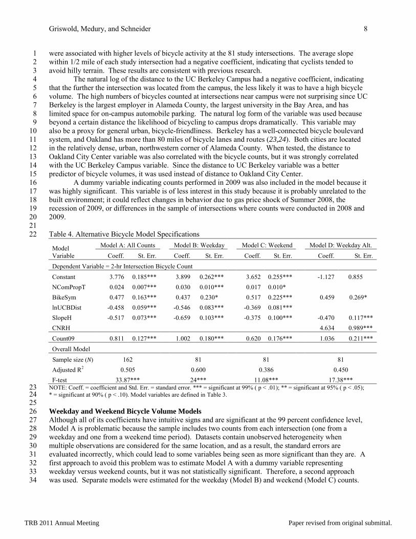
Factors Associated with Intersection Bicycle Volumes 25 Several options were considered during the model specification process. The models discussed are shown 26

in Table 4. While the adjusted R-square values varied among the models, the F-statistics showed that all 27

models were significant. Model A was the best fit model specification based on all counts (N = 162, F 28

=33.9). Number of retail commercial properties within 1/10 mile and presence of on-street bicycle 29

facilities both had positive coefficients in this model, indicating that retail activity and bicycle facilities 30



were associated with higher levels of bicycle activity at the 81 study intersections. The average slope 1

within 1/2 mile of each study intersection had a negative coefficient, indicating that cyclists tended to 2

avoid hilly terrain. These results are consistent with previous research. 3

The natural log of the distance to the UC Berkeley Campus had a negative coefficient, indicating 4

that the further the intersection was located from the campus, the less likely it was to have a high bicycle 5

volume. The high numbers of bicycles counted at intersections near campus were not surprising since UC 6

Berkeley is the largest employer in Alameda County, the largest university in the Bay Area, and has 7

limited space for on-campus automobile parking. The natural log form of the variable was used because 8

beyond a certain distance the likelihood of bicycling to campus drops dramatically. This variable may 9

also be a proxy for general urban, bicycle-friendliness. Berkeley has a well-connected bicycle boulevard 10

system, and Oakland has more than 80 miles of bicycle lanes and routes (23,24). Both cities are located 11

in the relatively dense, urban, northwestern corner of Alameda County. When tested, the distance to 12

Oakland City Center variable was also correlated with the bicycle counts, but it was strongly correlated 13

with the UC Berkeley Campus variable. Since the distance to UC Berkeley variable was a better 14

predictor of bicycle volumes, it was used instead of distance to Oakland City Center. 15

A dummy variable indicating counts performed in 2009 was also included in the model because it 16

was highly significant. This variable is of less interest in this study because it is probably unrelated to the 17

built environment; it could reflect changes in behavior due to gas price shock of Summer 2008, the 18

recession of 2009, or differences in the sample of intersections where counts were conducted in 2008 and 19

2009. 20

21

Table 4. Alternative Bicycle Model Specifications 22

Model

Variable

Model A: All Counts Model B: Weekday Model C: Weekend Model D: Weekday Alt.

Coeff. St. Err. Coeff. St. Err. Coeff. St. Err. Coeff. St. Err.

Dependent Variable = 2-hr Intersection Bicycle Count

Constant 3.776 0.185*** 3.899 0.262*** 3.652 0.255*** -1.127 0.855

NComPropT 0.024 0.007***

0.030 0.010***

0.017 0.010* BikeSym 0.477 0.163***

0.437 0.230*

0.517 0.225***

0.459 0.269*

lnUCBDist -0.458 0.059***

-0.546 0.083***

-0.369 0.081*** SlopeH -0.517 0.073***

-0.659 0.103***

-0.375 0.100***

-0.470 0.117***

CNRH

4.634 0.989***

Count09 0.811 0.127*** 1.002 0.180*** 0.620 0.176*** 1.036 0.211***

Overall Model

Sample size (N) 162 81 81 81

Adjusted R2 0.505

0.600

0.386

0.450

F-test 33.87*** 24*** 11.08*** 17.38***

NOTE: Coeff. = coefficient and Std. Err. = standard error. *** = significant at 99% ( p < .01); ** = significant at 95% ( p < .05); 23 * = significant at 90% ( p < .10). Model variables are defined in Table 3. 24 25

Weekday and Weekend Bicycle Volume Models 26 Although all of its coefficients have intuitive signs and are significant at the 99 percent confidence level, 27

Model A is problematic because the sample includes two counts from each intersection (one from a 28

weekday and one from a weekend time period). Datasets contain unobserved heterogeneity when 29

multiple observations are considered for the same location, and as a result, the standard errors are 30

evaluated incorrectly, which could lead to some variables being seen as more significant than they are. A 31

first approach to avoid this problem was to estimate Model A with a dummy variable representing 32

weekday versus weekend counts, but it was not statistically significant. Therefore, a second approach 33

was used. Separate models were estimated for the weekday (Model B) and weekend (Model C) counts. 34



As Table 4 shows, the weekday model (Model B) has the highest adjusted R-square (0.6) of the models 1

presented. The coefficients of Model B are similar to Model A, but the coefficient for the bicycle 2

markings is only significant at 90 percent. The weekend model (Model C), on the other hand, has a lower 3

adjusted R-square than Models A or B. While presence of bicycle markings is highly significant with a 4

larger coefficient, number of commercial properties is less significant with a smaller coefficient than in 5

the previous models. This result may have occurred because recreational bicycle trips are more common 6

on weekends, so the proximity of retail establishments may be less important for attracting weekend 7

bicycle activity. Bicycle markings could have a greater influence on weekends because bicyclists may 8

have more flexibility to seek routes with bicycle facilities or because less experienced riders who tend to 9

prefer marked bicycle facilities are more likely to ride on weekends. Model C also has smaller 10

coefficients for the UC Berkeley variable and the slope variable. This is consistent with the expectation 11

that fewer people would see the campus as a destination on the weekend and recreational riders might 12

seek out hilly terrain. 13

Finally, in consideration that Models A through C include a variable that is particular to this 14

Alameda County study area (lnUCBDist), a fourth model specification is presented. Model D is an 15

alternative weekday model that excludes the UC Berkeley variable. Model D also adds connected node 16

ratio within 1/2 mile and excludes the commercial property variable. As expected, connected node ratio 17

has a positive coefficient, meaning that areas with fewer dead end streets and cul-de-sacs have more 18

bicycle activity. Population density and employment density were included in a variety of model 19

specifications, but they did not perform well. Although these variables have been used in previous 20

studies, they were not included in the final set of bicycle volume models. 21

22

PRACTICAL APPLICATION 23 Practitioners wishing to apply an intersection bicycle volume model should select among Models B, C, 24

and D based on the type of counts being predicted (weekday or weekend) and their understanding of the 25

built environment in the study area. To extract counts from the models above the following formulation 26

should be used: 27

28

(2) 29

where: 30

Yi = predicted two-hour bicycle count at intersection i 31

Xji = value of explanatory variable j at intersection i 32

βj = model coefficient for variable j 33

34

When working with the loglinear form of a regression model, it is important to understand how to 35

interpret the coefficients correctly. They can be interpreted as the fractional increase in the bicycle 36

volume when the explanatory variable increases by 1 unit. Unlike OLS regression, the relationship 37

between coefficients, explanatory variables, and the predictions is nonlinear. For example, consider the 38

application of Model D to the median variable values for the set of 81 sample intersections. This model 39

produces a count prediction of 15 bicycles within a two-hour period on a typical weekday afternoon. The 40

median value of the connected node ratio variable (CNRH) in the sample is 0.85. Increasing the 41

coefficient of this variable from 4.634 to 5.634 brings the prediction up to 35.1 bicycles, an increase of 42

134 percent. Another unit increase in the coefficient raises the prediction to 82.4, more than five times 43

the original estimate. Along the same lines, examining the median values in Model B, a 20 percent 44

increase or decrease in the median value for SlopeH changes the predicted counts by -3 percent and 4 45

percent, respectively. Identical modifications to the median value for NComPropT change the predictions 46

by 36 percent and -26 percent, respectively. This sensitivity of the coefficients should be considered when 47

interpreting models. 48

49



CONSIDERATIONS FOR FUTURE RESEARCH 1 The models presented in this paper are preliminary and are not intended to be a final product. They 2

represent a first attempt at modeling bicycle volumes in one county in Northern California. Bicycle 3

activity in other communities is not expected to have an identical relationship to the built environment. 4

Additional models in other states and countries are needed to provide a more complete picture of how 5

surrounding land use, transportation system, and socioeconomic characteristics are related to bicycle 6

volumes at specific locations. One of the next steps for refining the Alameda County models is to collect 7

counts at additional locations and conduct model validation. 8

Ideally, the models would have been estimated using count data that was collected during the 9

same time-of-day at each location. In this case, however, counts were taken during different times of the 10

day on weekdays and Saturdays. In theory, the number of bicyclists passing through an intersection 11

between 12 p.m. and 2 p.m. on a given day is likely to be different than the number of bicyclists passing 12

through between 4 p.m. and 6 p.m. To account for these time-of-day differences, dummy variables 13

indicating the count time period were included in several versions of the models. However, the 14

coefficients of these variables were highly insignificant, indicating that controlling for time of day 15

provided little additional value for predicting bicycle volumes at the sample of 81 intersections. 16

Therefore, the time-of-day variables were not included in the models. Prior research on pedestrian 17

volumes in Alameda County dealt with this issue by using several months of automated pedestrian 18

counter data from several locations to extrapolate two-hour counts to weekly counts (21). Unfortunately, 19

since automated bicycle counters must be installed in a roadway, it is more difficult to collect counts from 20

a variety of locations or to capture both directions of a roadway. The available automated bicycle count 21

data from two locations in Alameda County could not be used for extrapolation without making gross 22

assumptions. 23

Weather effects were not incorporated into the final bicycle volume models. Dummy variables 24

indicating extreme temperatures and cloud cover proved highly insignificant in all model specifications. 25

This is likely due to the lack of variation in weather during the bicycle count periods. The count data 26

were collected in the spring months, and counts were rescheduled if it was raining. Alameda County has 27

a temperate climate, and there were only two counts on days where the temperature was greater than 90° 28

F (32° C) or less than 50° F (10° C). Weather is expected to show a greater effect on bicycle activity in 29

areas where the climate varies more. 30

Previous studies have found a significant relationship between the socioeconomic characteristics 31

of individuals and neighborhoods and likelihood of bicycling (14,17,25). In Alameda County, there was a 32

moderate correlation (0.3 < | ρ | < 0.5) between the bicycle counts and socioeconomic variables such as 33

surrounding neighborhood income (positive), percentage of rental housing (positive), and percentage of 34

residents under age 18 (negative). However, these variables were less significant than the built 35

environment variables in the final models, so they were not included. 36

In Alameda County, most retail and employment attractors are in the flatter areas, although the 37

hills are popular with recreational riders. A different set of study intersections could have included more 38

counts along popular recreational routes in the hills. This would likely have produced different model 39

results, particularly for the slope and proximity to retail variables. However, the 81 intersections were 40

selected to ensure representation from areas with different surrounding land uses, transportation 41

infrastructure, and neighborhood socioeconomic characteristics. Intersections were not chosen with the 42

specific intention to capture high bicycle volumes or popular bicycle routes. 43

The bicycle count dataset included only one zero-count occurrence. As mentioned above, this 44

value was changed to 0.1 so that the natural log could be computed. Since the motivation behind these 45

models is to provide reasonable estimates for planning purposes, rather than absolute accuracy, it is 46

acceptable to assume that a prediction of 0.1 represents no bicycle activity. This approach was expected 47

to have little effect on the models because it only applied to one count in the sample. Study areas with 48

less bicycle activity and multiple zero-count intersections would require a different model structure. 49

The independent variables included in the final models show statistically significant associations 50

between specific land use and transportation infrastructure characteristics and bicycle volumes. However, 51



they do not necessarily imply a causal relationship between any of the independent variables and levels of 1

bicycling. For example, adding a bicycle facility to an intersection approach may make the roadway a 2

more attractive place to ride, which could increase the bicycle volume at the intersection. However, 3

communities often add bicycle facilities to roadways that already have high bicycle volumes in order to 4

make conditions more comfortable for existing bicyclists. In this case, a high intersection bicycle volume 5

would precede the bicycle facility. Accordingly, these models are not intended to predict the change in 6

bicycle volume after installation of a bicycle facility. Instrumental variable methods could improve the 7

models by accounting for the potential endogeneity of the bicycle facility variable. 8

9

CONCLUSION 10 The preliminary models presented in this paper are simple tools that can be used to estimate bicycle 11

intersection counts during specific time periods. The analyses performed here contribute to the body of 12

research on relationships between the built environment and bicycle activity. In particular, the models 13

showed that bicycle volumes tended to be higher at intersections: 14

Surrounded by more commercial retail properties within 1/10 mile of the intersection 15

Closer to a major university 16

With a marked bicycle facility on at least one leg of the intersection 17

Surrounded by flatter terrain within 1/2 mile of the intersection 18

Surrounded by a more connected roadway network 19

In addition, the models showed several important differences between weekday and weekend intersection 20

bicycle volumes. The models showed that: 21

The positive influence of commercial retail establishments on bicycle volumes tended to be 22

greater on weekdays than on weekends 23

The positive influence of proximity to UC Berkeley tended to be greater on weekdays than on 24

weekends 25

The positive influence of bicycle facilities on bicycle volumes tended to be greater on weekends 26

than on weekdays 27

The negative influence of hilly terrain tended to be smaller on weekends than on weekdays 28

Further refinement and testing in other study areas is necessary to improve count predictions in 29

Alameda County or elsewhere. Bicycle volume counts are an important tool to help understand bicycle 30

crash risk and the impact of the built environment on travel. It is crucial to understand the level of bicycle 31

activity for bicycles to have a greater impact on funding and policy decisions. 32

33

ACKNOWLEDGEMENTS 34 The authors would like to thank Lindsay Arnold and David Ragland of UC Berkeley Safe Transportation 35

Research and Education Center (SafeTREC) for their assistance with the project. Special thanks to 36

Population Research Systems for collecting bicycle counts in Spring 2008 and to all of the volunteers 37

who collected bicycle counts in Spring 2009. This work was partially funded by the California 38

Department of Transportation and the Alameda County Transportation Improvement Authority. 39

40

REFERENCES 41 42

1. United States Census Bureau. 2006 American Community Survey 1-year Estimates. Available online: 43

http://factfinder.census.gov, 2007. 44

45

2. United States Census Bureau. 2008 American Community Survey 1-year Estimates. Available online: 46

http://factfinder.census.gov, 2009. 47

48

3. City of Portland, OR. Portland Bicycle Counts 2008. Available online: 49

http://www.portlandonline.com/shared/cfm/image.cfm?id=217489, October 2008. 50



1

4. New York City Department of Transportation. NYC Commuter Cycling Indicator. Available online: 2

http://www.nyc.gov/html/dot/downloads/pdf/commuter_cycling_indicator_and_data_2009.pdf, April 3

2009. 4

5

5. City of Seattle Department of Transportation. 2009 Downtown Bicycle Count Results. Available 6

online: http://www.cityofseattle.net/transportation/bikeinfo.htm, 2009. 7

8

6. San Francisco Municipal Transportation Agency. 2008 San Francisco State of Cycling Report. 9

Available online: http://www.sfmta.com/cms/bnews/documents/2008SFStateofCyclingReport.pdf, 2008. 10

11

7. Turner, S., G. Shunk, and A. Hottenstein. Development of a Methodology to Estimate Bicycle 12

and Pedestrian Travel Demand. Texas Transportation Institute, Research Project Number 0- 13

1723, Report 1723-S, Texas Department of Transportation, Federal Highway Administration, 14

September 1998. 15

16

8. Landis, B.W. The Bicycle System Performance Measures: The Intersection Hazard and 17

Latent Demand Score Models. ITE Journal, Vol. 66, No. 2, 1996, pp. 18-26. 18

19

9. City of Alexandria, VA. Alexandria Pedestrian and Bicycle Mobility Plan. Available online: 20

http://alexandriava.gov/localmotion/info/default.aspx?id=11418, June 2008. 21

22

10. Purvis, C. Incorporating Effects of Smart Growth and TOD in San Francisco Bay Area Travel 23

Demand Models: Current and Future Strategies. Metropolitan Transportation Commission, 24

Available Online: 25

http://www.mtc.ca.gov/maps_and_data/datamart/research/Incorporating_Smart_Growth_MTC_ 26

models.pdf, 2003. 27

28

11. Haynes, M. and S. Andrzejewski. GIS Based Bicycle & Pedestrian Demand Forecasting Techniques. 29

Travel Model Improvement Program Webinar. Available online: 30

http://tmip.fhwa.dot.gov/sites/tmip.fhwa.dot.gov/files/fehr_and_peers.pdf, April 29, 2010. 31

32

12. Jones, M., S. Ryan, J. Donlon, L. Ledbetter, D.R. Ragland, and L. Arnold. Seamless Travel: 33

Measuring Bicycle and Pedestrian Activity in San Diego County and its Relationship to Land Use, 34

Transportation, Safety, and Facility Type. Caltrans Task Order 6117. California Department of 35

Transportation, 2010. 36

37

13. McCahill, C. and N.W. Garrick. The Applicability of Space Syntax to Bicycle Facility Planning. In 38

Transportation Research Record: Journal of the Transportation Research Board, No. 2074, 39

Transportation Research Board of the National Academies, Washington, D.C., 2008, pp. 46–51. 40

41

14. Dill, J. and K. Voros. Factors Affecting Bicycling Demand: Initial Survey Findings from the Portland, 42

Oregon, Region. In Transportation Research Record: Journal of the Transportation Research Board, 43

No. 2031, Transportation Research Board of the National Academies, Washington, D.C., 2007, pp. 9–17. 44

45

15. Aultman-Hall, L., F.L. Hall, and B.B Baetz. Analysis of Bicycle Commuter Routes Using Geographic 46

Information Systems: Implications for Bicycle Planning. In Transportation Research Record: Journal of 47

the Transportation Research Board, No. 1578, Transportation Research Board of the National 48

Academies, Washington, D.C., 1997, pp. 102–110. 49

50



16. Dill J. and J. Gliebe. Understanding and Measuring Bicycling Behavior: A Focus on Travel Time and 1

Route Choice. OTREC-RR-08-03. Oregon Transportation Research and Education Consortium, 2

2008 3

4

17. Dill J. and T. Carr. Bicycle Commuting and Facilities in Major U.S. Cities: If You Build Them, 5

Commuters Will Use Them. In Transportation Research Record: Journal of the Transportation Research 6

Board, No. 1828, Transportation Research Board of the National Academies, Washington, D.C., 2003, 7

pp. 116–123. 8

9

18. Stinson, M.A. and C.R. Bhat. Commuter Bicyclist Route Choice: Analysis Using a Stated Preference 10

Survey. In Transportation Research Record: Journal of the Transportation Research Board, No. 1828, 11

Transportation Research Board of the National Academies, Washington, D.C., 2003, pp. 107–115. 12

13

19. Xing, Y., S.L. Handy, and T.J. Buehler. Factors Associated with Bicycle Ownership and Use: A 14

Study of 6 Small U.S. Cities. Presented at 87th Annual Meeting of the Transportation Research Board, 15

Washington, D.C., 2008. 16

17

20. W.W. Hunter, L. Thomas and J.C. Stutts. BIKESAFE : Bicycle Countermeasure Selection System. 18

FHWA-SA-05-006. FHWA, U.S. Department of Transportation, 2006. 19

20

21. Schneider R.J., L.S. Arnold, and D.R. Ragland. Pilot Model for Estimating Pedestrian: Intersection 21

Crossing Volumes. In Transportation Research Record: Journal of the Transportation Research Board, 22

No. 2140, Transportation Research Board of the National Academies, Washington, D.C., 2009, pp. 13–23

26. 24

25

22. Schneider R.J., M.C. Diogenes L.S. Arnold, V. Attaset, J. Griswold, and D.R. Ragland. Association 26

between Roadway Intersection Characteristics and Pedestrian Crash Risk in Alameda County, California. 27

Forthcoming, Transportation Research Record: Journal of the Transportation Research Board, 2010. 28

29

23. City of Berkeley Transportation Division. Bicycle Boulevards in Berkeley. Available online: 30

http://www.ci.berkeley.ca.us/ContentDisplay.aspx?id=6650, 2010. 31

32

24. City of Oakland Public Works Agency. City of Oakland Pedestrian and Bicycling Information. 33

Available online: http://www.oaklandpw.com/Page122.aspx, 2010. 34

35

25. Xing, Y., S.L. Handy, and T.J. Buehler. Factors Associated with Bicycle Ownership and Use: 36

A Study of 6 Small U.S. Cities. University of California, Davis, Available online, 37

http://www.des.ucdavis.edu/faculty/handy/TTP_seminar/Bike_Draft_11.14.pdf, 2008. 38

39



LIST OF TABLES AND FIGURES

TABLES

Table 1. Factors Associated with Bicycling in Previous Research Table 2. Summary Statistics for all Two-Hour Bicycle Counts Table 3. Description of Selected Explanatory Variables Considered in the Modeling Process Table 4. Alternative Bicycle Model Specifications

FIGURES

Figure 1. Map of Manual Bicycle Count Locations


Pilot Models for Estimating Bicycle Intersection Volumes

Documents