Metaheuristic Computing and Applications, Vol. 1, No. 2 (2020) 165-186 DOI: https://doi.org/10.12989/mca.2020.1.2.165 165 Copyright © 2020 Techno-Press, Ltd. http://www.techno-press.org/?journal=mca&subpage=5 ISSN: 2713-5519 (Print), 2733-8053 (Online) Pile bearing capacity estimation using GEP, RBFNN and MVNR techniques Hooman Harandizadeh 1 , Danial Jahed Armaghani 2 and Vahid Toufigh 3 1 Department of Civil Engineering. Faculty of Engineering. Shahid Bahonar University of Kerman. Pajoohesh Sq. Imam Khomeni Highway. P.O. Box 76169133. Kerman, Iran 2 Department of Civil Engineering. Faculty of Engineering. University of Malaya. 50603. Kuala Lumpur, Malaysia 3 Faculty of Civil and Surveying Engineering. Graduate University of Advanced Technology. Kerman, Iran (Received March 18, 2020, Revised August 19, 2020, Accepted December 22, 2020) Abstract. This study introduced a new predictive approach for estimating the bearing capacity of driven piles. To this end, the required data based on literature such as hammer strikes, soil properties, geometry of the pile, and friction angle between pile and soil were gathered as a suitable database. Then, three predictive models i.e., gene expression programming (GEP), radial basis function type neural networks (RBFNN) and multivariate nonlinear regression (MVNR) were applied and developed for pile bearing capacity prediction. After proposing new models, their performance indices i.e., root mean square error (RMSE) and coefficient of determination (R2) were calculated and compared to each other in order to select the best one among them. The obtained results indicated that the RBFNN model is able to provide higher performance prediction level in comparison with other predictive techniques. In terms of R2, results of 0.9976, 0.9466 and 0.831 were obtained for RBFNN, GEP and MVNR models respectively, which confirmed that, the developed RBFNN model could be selected as a new model in piling technology. Definitely, other researchers and engineers can utilize the procedure and results of this study in order to get better design of driven piles. Keywords: pile bearing capacity; radial basis function type artificial neural networks (RBFNN); multivariate nonlinear regression (MVNR); gene expression programming (GEP) 1. Introduction A commonly-encountered problem in foundation design is the accurate prediction of the ultimate capacity of load bearing in case of each driven pile used in the project (Samui 2012, Samui and Kim 2013, Khari et al. 2019a, Momeni et al. 2020). It is true that in similar geotechnical conditions, the same bearing capacity equation is usually applied to various piles set up; however, this needs to be done very cautiously. Likewise, as the pile-soil interactions are not clear, most of the methods (already introduced in literature) fail to predict the pile capacity accurately (Meschke et al. 2013, Wu et al. 2019). Such failure can be due to simplifications and assumptions they normally take into account when interpreting behaviors of pile (Harandizadeh et al. 2018). The use of existing static solutions for the aim of determining the bottom resistance can Corresponding author, Senior Lecturer, E-mail: [email protected]

Welcome message from author
This document is posted to help you gain knowledge. Please leave a comment to let me know what you think about it! Share it to your friends and learn new things together.
Transcript

Metaheuristic Computing and Applications, Vol. 1, No. 2 (2020) 165-186
DOI: https://doi.org/10.12989/mca.2020.1.2.165 165
Copyright © 2020 Techno-Press, Ltd.
http://www.techno-press.org/?journal=mca&subpage=5 ISSN: 2713-5519 (Print), 2733-8053 (Online)
Pile bearing capacity estimation using GEP, RBFNN and MVNR techniques
Hooman Harandizadeh1, Danial Jahed Armaghani2 and Vahid Toufigh3
1Department of Civil Engineering. Faculty of Engineering. Shahid Bahonar University of Kerman. Pajoohesh Sq. Imam Khomeni Highway. P.O. Box 76169133. Kerman, Iran
2Department of Civil Engineering. Faculty of Engineering. University of Malaya. 50603. Kuala Lumpur, Malaysia
3Faculty of Civil and Surveying Engineering. Graduate University of Advanced Technology. Kerman, Iran
(Received March 18, 2020, Revised August 19, 2020, Accepted December 22, 2020)
Abstract. This study introduced a new predictive approach for estimating the bearing capacity of driven piles. To this end, the required data based on literature such as hammer strikes, soil properties, geometry of the pile, and friction angle between pile and soil were gathered as a suitable database. Then, three predictive models i.e., gene expression programming (GEP), radial basis function type neural networks (RBFNN) and multivariate nonlinear regression (MVNR) were applied and developed for pile bearing capacity prediction. After proposing new models, their performance indices i.e., root mean square error (RMSE) and coefficient of determination (R2) were calculated and compared to each other in order to select the best one among them. The obtained results indicated that the RBFNN model is able to provide higher performance prediction level in comparison with other predictive techniques. In terms of R2, results of 0.9976, 0.9466 and 0.831 were obtained for RBFNN, GEP and MVNR models respectively, which confirmed that, the developed RBFNN model could be selected as a new model in piling technology. Definitely, other researchers and engineers can utilize the procedure and results of this study in order to get better design of driven piles.
Keywords: pile bearing capacity; radial basis function type artificial neural networks (RBFNN);
multivariate nonlinear regression (MVNR); gene expression programming (GEP)
1. Introduction
A commonly-encountered problem in foundation design is the accurate prediction of the
ultimate capacity of load bearing in case of each driven pile used in the project (Samui 2012,
Samui and Kim 2013, Khari et al. 2019a, Momeni et al. 2020). It is true that in similar
geotechnical conditions, the same bearing capacity equation is usually applied to various piles set
up; however, this needs to be done very cautiously. Likewise, as the pile-soil interactions are not
clear, most of the methods (already introduced in literature) fail to predict the pile capacity
accurately (Meschke et al. 2013, Wu et al. 2019). Such failure can be due to simplifications and
assumptions they normally take into account when interpreting behaviors of pile (Harandizadeh et
al. 2018). The use of existing static solutions for the aim of determining the bottom resistance can
Corresponding author, Senior Lecturer, E-mail: [email protected]
Hooman Harandizadeh, Danial Jahed Armaghani and Vahid Toufigh
result in a similar convenience of different piles of a task. On the other hand, prevailing
equations and methods of high efficiency normally take into account the over-simplification of the
pile traveling problem (Samui 2008, Chen et al. 2019b). These methods mostly employ the
information regarding pile and hammer in the prediction of the pile capacity. However, the soil
characteristics are not considered in these methods. Lastly, despite the fact that static assessments
are the most reliable strategy among all, they also suffer from limitations. For instance, in cases
where the pile loading stops before failure of the pile, it will be difficult to interpret the test results.
On the other hand, when loading is continued before failure of the pile, the check piles get
impaired, and experiments can be applied to only a few piles. Add to the above-mentioned points
the fact that such checks are very costly (Momeni et al. 2015a, Harandizadeh et al. 2019b). As a
result, there is a need for a well-standardized technique capable of accurately estimating the
compressive bearing capacity of each driven pile. Numerous parameters affect the calculation of
bearing capacity of the piles; thus, efficient computational algorithms are necessary to effectively
explore and control the interactions among the effective parameters. The techniques with no need
for any prior assumption, e.g., artificial intelligence (AI) and machine learning (ML) techniques
can provide solutions of a higher quality. Literature confirms the extensive application of AI and
ML techniques such as genetic programming (GP), particle swarm optimization (PSO), adoptive
neuro fuzzy inference system (ANFIS), gene expression programming (GEP) and artificial neural
network (ANN) in civil engineering as well as geotechnical fields (Momeni et al. 2013,
Najafzadeh and Azamathulla 2013, Najafzadeh et al. 2013, Toghroli et al. 2014, Yang et al. 2014,
2016, 2018, Najafzadeh 2015, Das and Suman 2015, Najafzadeh and Bonakdari 2016, Zhou et al.
2016, 2019, 2020a, 2020b, 2020c, Asteris et al. 2017, 2019, Kechagias et al. 2018, Koopialipoor et
al. 2018, Wang et al. 2018, Bunawan et al. 2018, Apostolopoulou et al. 2019, Armaghani et al.
2019a, Hajihassani et al. 2019, Huang et al. 2019, Khari et al. 2019b, Armaghani et al. 2019b,
Sarir et al. 2019, Xu et al. 2019a, 2019b, Armaghani et al. 2020a, Zhang et al. 2019, Chen et al.
2019a, Duan et al. 2020, Lu et al. 2020, Armaghani et al. 2020). In case of piling technology, a
variety of input parameters have been considered by different scholars in modelling processes
making attempt to estimate the bearing capacity of piles with a maximum level of accuracy
(Momeni et al. 2014, 2015b, 2018, Armaghani et al. 2017).
Chan et al. (1995) employed a back-propagation neural network (BPNN) containing three
layers in order to examine the driven piles bearing capacity with the help of the input parameters
i.e., the elastic compression of soil and pile, pile setup, and generating energy used in a pile. They
showed a successful use of BPNN technique in predicting pile bearing capacity. In another study
of ANN, Lee and Lee (1996) used this technique for the purpose of estimating their experimental
piles bearing capacity in addition to a number of full-level pile load tests extracted through a
literature review. Their assumption was that the highest bearing capacities had suffered from some
issues such as the ratio of penetration depth, the averaged regular penetration number close to the
pile tip, the averaged regular penetration quantity along the pile shaft, pile arranged (last
penetration depth/blow), as well as the hammer energy. Abu Kiefa (1998) attempted to propose a
regression ANN capable of estimating a driven pile capacity within non-cohesive soil. He set four
parameters as model inputs to his model, namely the soil friction angle, effective overburden
pressure, duration of pile, and the cross-sectional region of the pile. Ardalan et al. (2009) made use
of the group method of data handling (GMDH) model optimized by genetic algorithm (GA). Their
input parameters were cone resistance and cone sleeve friction, and the pile shaft resistance. To
this end, they utilized a data source containing 33 full-level pile loading lab tests accompanied
with details of soil types and the cone penetration tests (CPTs), which were carried out nearby the
166
Pile bearing capacity estimation using GEP. RBFNN and MVNR techniques
location of the piles. In another study, Alkroosh and Nikraz (2012) developed a GEP equation for
the prediction of the capacity of piles driven into cohesive soil. Their model utilized a number of
independent variables such as the length and size of piles, weighted sleeve friction along the pile
shaft, pile materials, and pile elastic modulus Data required for developing GEP model were
gathered from the related literature involving a number of in-situ assessment of driven pile load
and results obtained from the CPTs. Some other techniques e.g., PSO-ANN, GA-ANN, ICA-ANN,
ANFIS-GMDH-PSO, and GP were introduced in the studies by Armaghani et al. (2017), Momeni
et al. (2014), Moayedi and Armaghani (2018), Harandizadeh et al. (2019a), and Chen et al.
(2019b), respectively, as the best predictive models of the pile ultimate capacity.
To effectively model the pile bearing capacity, the above-mentioned studies mainly made use of
parameters such as pile setup, cone tip resistance, or N- standard penetration test (SPT) values.
However, based on previous investigations, the number of hammer blows should be taken into
consideration as the key parameter in the process of measuring the driven piles’ ultimate bearing
capacity. In this respect, the Flap number refers to the number of hammer blows used in order to
drive into the soil the last one meter of remaining length of the pile. The value set for this case is a
unique number for each one of the piles; it actually reflects the conditions of the soil and the way
pile and soil interact with each other. Note that the Flap number greatly depends upon the type of
hammer in use. As a result, the number of blows is multiplied by the hammer relative energy in a
way to make a comparison on the level of blows each pile received.
In addition, in most of previously-conducted studies, it was assumed that the soil physical
parameters do not work in a pile, whereas in the present study, not only the Flap hammer blows
number, but also the soil parameters, geometric parameters of the piles, and the friction angle
between pile and soil were taken into account as significant factors. To carry out a wide-ranging
study, a dataset containing 100 piles (made from steel and concrete) was provided. Additionally,
the information in regard to the soil conditions and the results obtained from field tests were
considered as effective parameters on piling capacity. The data collected for the purpose of this
study included various steel and concrete piles whose length was ranging from 15 m to 98 m.
In this study, initially, the method of radial basis function type neural networks (RBFNN) was
employed to predict ultimate bearing capacity of the piles. Then, the GEP was used in a way to
obtain an equation for predicting the capacity of pile from the Flap number and the other effective
factors. At the final step, another method termed multivariate nonlinear regression (MVNR) was
adopted for the estimation of pile capacity. The coefficient of determination (R2) and root mean
square error (RMSE) were used to test the precision level of the results obtained from each
approach adopted. Then, the best predictive model among them was selected to predict pile
bearing capacity.
2. Pile information and data used
For the purpose of this research, a database containing of 100 concrete and steel piles were
taken into consideration. In each of them, information including the ground physical properties,
the geometrical characteristics, static pile load test outputs, Flap number (the number of hammer
strikes), and their particular hammer strike energies were gathered. The assumption was that
factors such as the soil drained cohesion, friction angle of soil drained, and specific weight affect
the conditions of soil. The two parameters of embedded duration and pile cross section refer to the
pile geometric size and, on the other hand, the pile-soil friction position affects the pile material.
167
Hooman Harandizadeh, Danial Jahed Armaghani and Vahid Toufigh
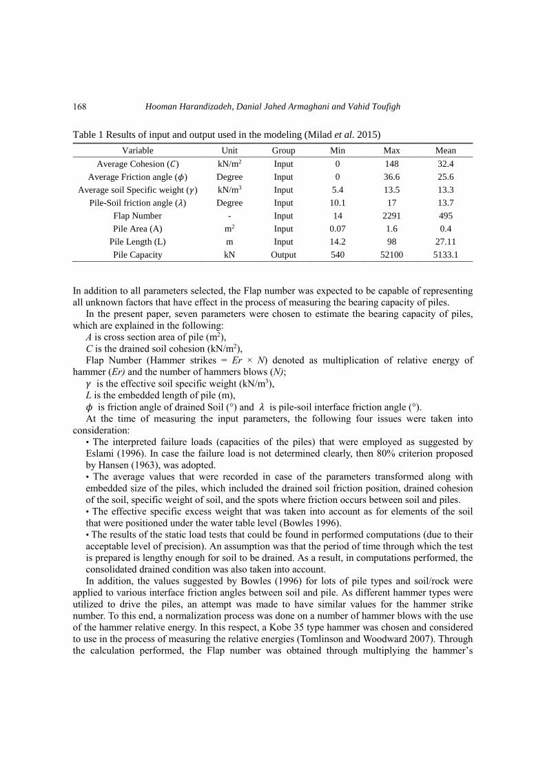
Table 1 Results of input and output used in the modeling (Milad et al. 2015)
Variable Unit Group Min Max Mean
Average Cohesion (𝐶) kN/m2 Input 0 148 32.4
Average Friction angle (𝜙) Degree Input 0 36.6 25.6
Average soil Specific weight (𝛾) kN/m3 Input 5.4 13.5 13.3
Pile-Soil friction angle (𝜆) Degree Input 10.1 17 13.7
Flap Number - Input 14 2291 495
Pile Area (A) m2 Input 0.07 1.6 0.4
Pile Length (L) m Input 14.2 98 27.11
Pile Capacity kN Output 540 52100 5133.1
In addition to all parameters selected, the Flap number was expected to be capable of representing
all unknown factors that have effect in the process of measuring the bearing capacity of piles.
In the present paper, seven parameters were chosen to estimate the bearing capacity of piles,
which are explained in the following:
A is cross section area of pile (m2),
C is the drained soil cohesion (kN/m2),
Flap Number (Hammer strikes = Er × N) denoted as multiplication of relative energy of
hammer (Er) and the number of hammers blows (N);
𝛾 is the effective soil specific weight (kN/m3),
L is the embedded length of pile (m),
𝜙 is friction angle of drained Soil (°) and 𝜆 is pile-soil interface friction angle (°).
At the time of measuring the input parameters, the following four issues were taken into
consideration:
• The interpreted failure loads (capacities of the piles) that were employed as suggested by
Eslami (1996). In case the failure load is not determined clearly, then 80% criterion proposed
by Hansen (1963), was adopted.
• The average values that were recorded in case of the parameters transformed along with
embedded size of the piles, which included the drained soil friction position, drained cohesion
of the soil, specific weight of soil, and the spots where friction occurs between soil and piles.
• The effective specific excess weight that was taken into account as for elements of the soil
that were positioned under the water table level (Bowles 1996).
• The results of the static load tests that could be found in performed computations (due to their
acceptable level of precision). An assumption was that the period of time through which the test
is prepared is lengthy enough for soil to be drained. As a result, in computations performed, the
consolidated drained condition was also taken into account.
In addition, the values suggested by Bowles (1996) for lots of pile types and soil/rock were
applied to various interface friction angles between soil and pile. As different hammer types were
utilized to drive the piles, an attempt was made to have similar values for the hammer strike
number. To this end, a normalization process was done on a number of hammer blows with the use
of the hammer relative energy. In this respect, a Kobe 35 type hammer was chosen and considered
to use in the process of measuring the relative energies (Tomlinson and Woodward 2007). Through
the calculation performed, the Flap number was obtained through multiplying the hammer’s
168
Pile bearing capacity estimation using GEP. RBFNN and MVNR techniques
relative energy and the number of blows (Prakash and Sharma 1990). Table 1 presents descriptions
of all 100 input and output variables (Milad et al. 2015) used in the modeling process of this study.
3. Applied methods
3.1 Radial basis function type neural networks (RBFNN)
ANNs are common in the application of geotechnical research problems due to giving an
interesting approach for modeling phenomenon’s behavior. In recent years, different types of
ANNs have been efficiently used to simulate different soil behaviors such as compaction of soil
(Sinha and Wang 2008), soil liquefaction (Young-Su and Byung-Tak 2006), and thermal properties
of soil (Erzin et al. 2008). They also utilized to the model arrangement of shallow fundamentals
(Shahin et al. 2002), tension- stress behavior of sandy soil (Banimahd et al. 2005), and earth
category fields (Kurup and Griffin 2006). Literature consists of numerous studies in which ANNs
have been utilized aiming at determining the capacity of piles (Kiefa 1998; Alkroosh and Nikraz
2012). The method that was the first one applied to the prediction of the piles’ bearing capacity
with the use of their hammer strike and other effective factors was the Radial Basis Function
Neural Network (RBFNN).
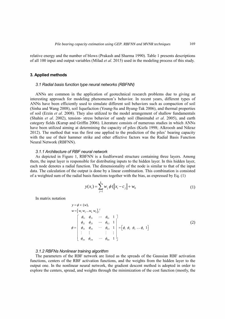
3.1.1 Architecture of RBF neural network As depicted in Figure 1, RBFNN is a feedforward structure containing three layers. Among
them, the input layer is responsible for distributing inputs to the hidden layer. In this hidden layer,
each node denotes a radial function. The dimensionality of the node is similar to that of the input
data. The calculation of the output is done by a linear combination. This combination is consisted
of a weighted sum of the radial basis functions together with the bias, as expressed by Eq. (1)
(1)
In matrix notation
(2)
3.1.2 RBFNs Nonlinear training algorithm The parameters of the RBF network are listed as the spreads of the Gaussian RBF activation
functions, centers of the RBF activation functions, and the weights from the hidden layer to the
output one. In the nonlinear neural network, the gradient descent method is adopted in order to
explore the centers, spread, and weights through the minimization of the cost function (mostly, the
0
1
( ) (k
i j i j
j
y x w x c w
1 2 0
11 21 1
12 23 2
13 23 3 1 2 3
1 2
( ),
... ,
1
1
1 1
1
T
k
k
k
k k
m m km
y w
w w w w w
169

Hooman Harandizadeh, Danial Jahed Armaghani and Vahid Toufigh
Fig. 1 RBF type neural network structure
squared error). The network parameters are adapted by the BP algorithm. This algorithm takes into
consideration the cost function derivatives upon the parameters in an iterative process. The
challenging issue is that the BP probably needs a number of iterations, and also this algorithm
might be trapped in the cost function local minima (Asteris et al. 2016, 2019, 2020,
Apostolopoulou et al. 2020, Armaghani et al. 2020b, Armaghani and Asteris 2020, Asteris, et al.
2020).
Divisions in Dataset Sampling
For the purpose of computations required, the samples were divided into two groups:
• Training set (70% Samples): The samples in this group were used to locate the neural system
biases and weights in a way to reduce the error value as much as possible. Such samples are
applied to the network in the course of the overall training. The error value obtained was used
to adjust the system.
• Testing set (30% Samples): The samples in this group were applied to the assessment of the
neural system with the best weights explored throughout the training process; the accuracy
level was also measured in this course. Such samples do not affect the appropriate training; as a
result, they can make available an unbiased way to evaluate the way the network performs both
after and during the training process.
3.2 Gene Expression Programming (GEP) 3.2.1 GEP structural concepts GEP is actually an extended version of the GA that is an evolutionary optimization algorithm
works according to the genetics principles and natural selection theory. The evolutionary
processing technique is GP that was introduced by (Koza 1992). This algorithm is applied to
representing systematically the information provided through the manipulation and optimization of
a network of computer models made up of terminals and functions in a way to be capable of
searching for a model that can be best matched with the problem in hand. GP is defined as a
domain-independent approach to solving problems. It creates computer programs involving a
number of different terminals and features for the aim of solving the approximation problems
through simulating the living organisms’ biological evolutions and genetic operations that occur in
170
Pile bearing capacity estimation using GEP. RBFNN and MVNR techniques
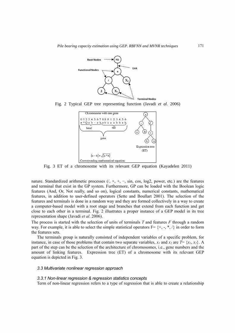
Fig. 2 Typical GEP tree representing function (Javadi et al. 2006)
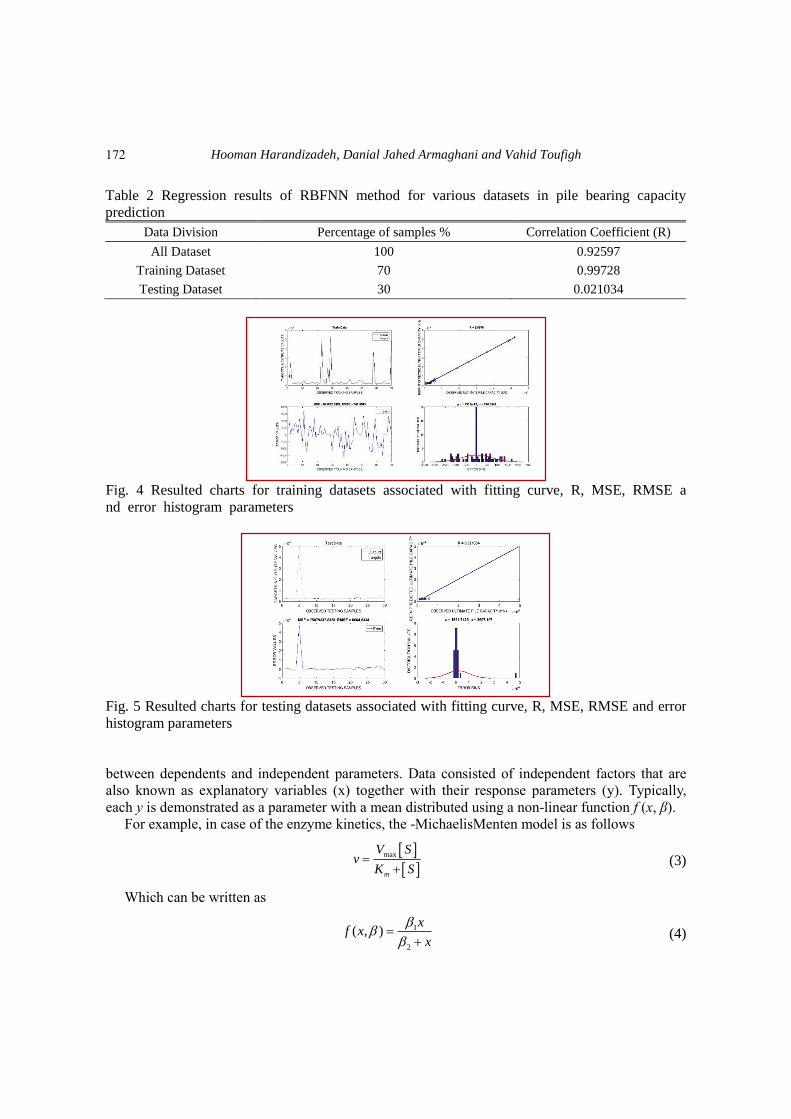
Fig. 3 ET of a chromosome with its relevant GEP equation (Kayadelen 2011)
nature. Standardized arithmetic processes (/, ×, +, −, sin, cos, log2, power, etc.) are the features
and terminal that exist in the GP system. Furthermore, GP can be loaded with the Boolean logic
features (And, Or, Not really, and so on), logical constants, numerical constants, mathematical
features, in addition to user-defined operators (Sette and Boullart 2001). The selection of the
features and terminals is done in a random way and they are formed collectively in a way to create
a computer-based model with a root stage and branches that extend from each function and get
close to each other in a terminal. Fig. 2 illustrates a proper instance of a GEP model in its tree
representation shape (Javadi et al. 2006).
The process is started with the selection of units of terminals T and features F through a random
way. For example, it is able to select the simple statistical operators F= {+, -, *, /} in order to form
the features sets.
The terminals group is naturally consisted of independent variables of a specific problem, for
instance, in case of those problems that contain two separate variables, x1 and x2 are T= {x1, x2}. A
part of the step can be the selection of the architecture of chromosomes, i.e., gene numbers and the
amount of linking features. Expression tree (ET) of a chromosome with its relevant GEP
equation is depicted in Fig. 3.
3.3 Multivariate nonlinear regression approach
3.3.1 Non-linear regression & regression statistics concepts Term of non-linear regression refers to a type of regression that is able to create a relationship
171
Hooman Harandizadeh, Danial Jahed Armaghani and Vahid Toufigh
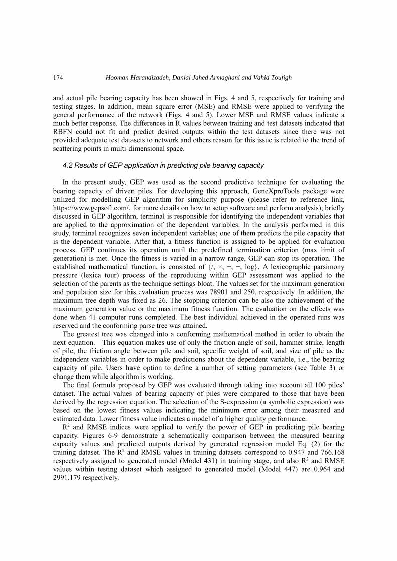
Table 2 Regression results of RBFNN method for various datasets in pile bearing capacity
prediction
Data Division Percentage of samples % Correlation Coefficient (R)
All Dataset 100 0.92597
Training Dataset 70 0.99728
Testing Dataset 30 0.021034
Fig. 4 Resulted charts for training datasets associated with fitting curve, R, MSE, RMSE a
nd error histogram parameters
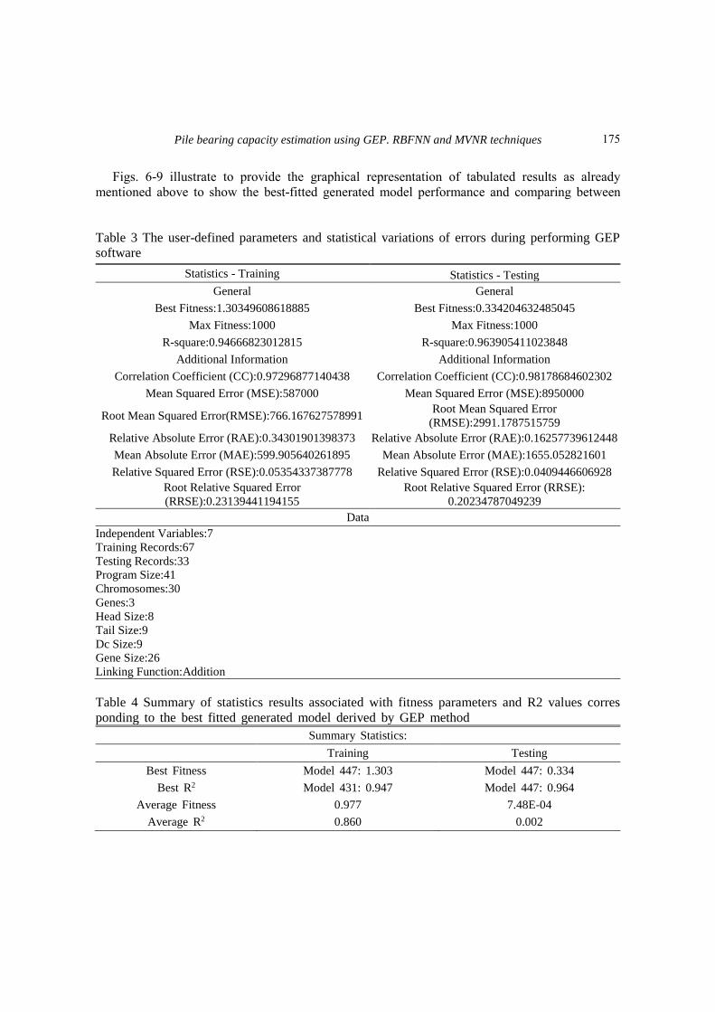
Fig. 5 Resulted charts for testing datasets associated with fitting curve, R, MSE, RMSE and error
histogram parameters
between dependents and independent parameters. Data consisted of independent factors that are
also known as explanatory variables (x) together with their response parameters (y). Typically,
each y is demonstrated as a parameter with a mean distributed using a non-linear function f (x, β).
For example, in case of the enzyme kinetics, the -MichaelisMenten model is as follows
(3)
Which can be written as
(4)
max
m
V Sv
K S
1
2
( , )x
f xx
172

Pile bearing capacity estimation using GEP. RBFNN and MVNR techniques
where β1 stands for the parameter Vmax, β2 denotes the parameter Km, and [S] signifies the
independent variable (x). The nonlinearity of this function is clear since it cannot be articulated as
a linear combination of the two βs. Some other types of non-linear functions are logarithmic
functions, exponential functions, Gaussian function, power features, Lorenz curves, and
trigonometric features. Unlike the linear regression, many regional minima of function can appear
to be optimized, and the global minimum quantity can lead to the formation of a biased estimation.
The predicted values of parameters are applied to optimization algorithms in order to explore the
least sum of squares.
The assumption underlying this process is that a linear function could approximate the model as
following
where . It follows from this that the least squares estimators are given by
Non-linear regression statistics are computed and employed similar to those in the linear
regression statistics; however, in formulas adopted in this process, J is used in place of X. Linear
approximation introduces bias to the statistics. As a result, it is needed to be very cautious in the
interpretation of the statistics generated from nonlinear models.
4. Results and discussions 4.1 Results of RBFNN application in predicting pile bearing capacity In case of the neural system, the MATLAB software chooses 70% of the total datasets for the
training purposes in an automatic and appropriate way. The remaining 30% of the datasets were
dedicated to testing purposes. These samples are also chosen in a random way. To attain the RBF
network outcomes, the seven effective input parameters need to be ordered as offered in the
following column matrix:
𝐼𝑛𝑝𝑢𝑡 𝑀𝑎𝑡𝑟𝑖𝑥 = [𝐶 𝜙 𝛾 𝜆 𝐹𝑙𝑎𝑝 𝐴 𝐿]′
In the term of , p refers to the input matrix, b, and w present bias and weight
matrices, respectively, the results of RBF can be calculated from the first layer to the last one. In
this way, the bearing capacity of the pile can be calculated using the RBFN technique.
The correlation coefficient, i.e., the regression determination coefficient, which is signified by
R, was applied to the measurement of the success rate of the RBF type neural network regarding
the prediction of the piles’ capacity. The coefficient reveals the variation percentage within the
datasets; the obtained value ranges from 0 to 1. When the value of R is closer to 1, this means the
model is well-matched with the data; on the other hand, when this value is closer to 0, it means the
model is not matched well with the data perfectly. Table 2 shows these values for all three datasets
(all samples, training samples, test samples). Assessment of RBF neural network predicted outputs
( , )iij
j
f xJ
"a= ( )"f wp b
(5)
(6)
0( , )i ij j
j
f x f J
1ˆ ( )T TJ J J y
173
Hooman Harandizadeh, Danial Jahed Armaghani and Vahid Toufigh
and actual pile bearing capacity has been showed in Figs. 4 and 5, respectively for training and
testing stages. In addition, mean square error (MSE) and RMSE were applied to verifying the
general performance of the network (Figs. 4 and 5). Lower MSE and RMSE values indicate a
much better response. The differences in R values between training and test datasets indicated that
RBFN could not fit and predict desired outputs within the test datasets since there was not
provided adequate test datasets to network and others reason for this issue is related to the trend of
scattering points in multi-dimensional space.
4.2 Results of GEP application in predicting pile bearing capacity
In the present study, GEP was used as the second predictive technique for evaluating the
bearing capacity of driven piles. For developing this approach, GeneXproTools package were
utilized for modelling GEP algorithm for simplicity purpose (please refer to reference link,
https://www.gepsoft.com/, for more details on how to setup software and perform analysis); briefly
discussed in GEP algorithm, terminal is responsible for identifying the independent variables that
are applied to the approximation of the dependent variables. In the analysis performed in this
study, terminal recognizes seven independent variables; one of them predicts the pile capacity that
is the dependent variable. After that, a fitness function is assigned to be applied for evaluation
process. GEP continues its operation until the predefined termination criterion (max limit of
generation) is met. Once the fitness is varied in a narrow range, GEP can stop its operation. The
established mathematical function, is consisted of {/, ×, +, −, log}. A lexicographic parsimony
pressure (lexica tour) process of the reproducing within GEP assessment was applied to the
selection of the parents as the technique settings bloat. The values set for the maximum generation
and population size for this evaluation process was 78901 and 250, respectively. In addition, the
maximum tree depth was fixed as 26. The stopping criterion can be also the achievement of the
maximum generation value or the maximum fitness function. The evaluation on the effects was
done when 41 computer runs completed. The best individual achieved in the operated runs was
reserved and the conforming parse tree was attained. The greatest tree was changed into a conforming mathematical method in order to obtain the
next equation. This equation makes use of only the friction angle of soil, hammer strike, length
of pile, the friction angle between pile and soil, specific weight of soil, and size of pile as the
independent variables in order to make predictions about the dependent variable, i.e., the bearing
capacity of pile. Users have option to define a number of setting parameters (see Table 3) or
change them while algorithm is working.
The final formula proposed by GEP was evaluated through taking into account all 100 piles’
dataset. The actual values of bearing capacity of piles were compared to those that have been
derived by the regression equation. The selection of the S-expression (a symbolic expression) was
based on the lowest fitness values indicating the minimum error among their measured and
estimated data. Lower fitness value indicates a model of a higher quality performance.
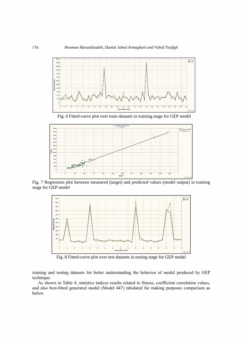
R2 and RMSE indices were applied to verify the power of GEP in predicting pile bearing
capacity. Figures 6-9 demonstrate a schematically comparison between the measured bearing
capacity values and predicted outputs derived by generated regression model Eq. (2) for the
training dataset. The R2 and RMSE values in training datasets correspond to 0.947 and 766.168
respectively assigned to generated model (Model 431) in training stage, and also R2 and RMSE
values within testing dataset which assigned to generated model (Model 447) are 0.964 and
2991.179 respectively.
174
Pile bearing capacity estimation using GEP. RBFNN and MVNR techniques
Figs. 6-9 illustrate to provide the graphical representation of tabulated results as already
mentioned above to show the best-fitted generated model performance and comparing between
Table 3 The user-defined parameters and statistical variations of errors during performing GEP
software
Statistics - Training Statistics - Testing
General General
Best Fitness:1.30349608618885 Best Fitness:0.334204632485045
Max Fitness:1000 Max Fitness:1000
R-square:0.94666823012815 R-square:0.963905411023848
Additional Information Additional Information
Correlation Coefficient (CC):0.97296877140438 Correlation Coefficient (CC):0.98178684602302
Mean Squared Error (MSE):587000 Mean Squared Error (MSE):8950000
Root Mean Squared Error(RMSE):766.167627578991 Root Mean Squared Error
(RMSE):2991.1787515759
Relative Absolute Error (RAE):0.34301901398373 Relative Absolute Error (RAE):0.16257739612448
Mean Absolute Error (MAE):599.905640261895 Mean Absolute Error (MAE):1655.052821601
Relative Squared Error (RSE):0.05354337387778 Relative Squared Error (RSE):0.0409446606928
Root Relative Squared Error
(RRSE):0.23139441194155
Root Relative Squared Error (RRSE):
0.20234787049239
Data
Independent Variables:7
Training Records:67
Testing Records:33
Program Size:41
Chromosomes:30
Genes:3
Head Size:8
Tail Size:9
Dc Size:9
Gene Size:26
Linking Function:Addition
Table 4 Summary of statistics results associated with fitness parameters and R2 values corres
ponding to the best fitted generated model derived by GEP method
Summary Statistics:
Training Testing
Best Fitness Model 447: 1.303 Model 447: 0.334
Best R2 Model 431: 0.947 Model 447: 0.964
Average Fitness 0.977 7.48E-04
Average R2 0.860 0.002
175
Hooman Harandizadeh, Danial Jahed Armaghani and Vahid Toufigh
Fig. 6 Fitted-curve plot over train datasets in training stage for GEP model
Fig. 7 Regression plot between measured (target) and predicted values (model output) in training
stage for GEP model
Fig. 8 Fitted-curve plot over test datasets in testing stage for GEP model
training and testing datasets for better understanding the behavior of model produced by GEP
technique.
As shown in Table 4, statistics indices results related to fitness, coefficient correlation values,
and also best-fitted generated model (Model 447) tabulated for making purposes comparison as
below.
176
Pile bearing capacity estimation using GEP. RBFNN and MVNR techniques
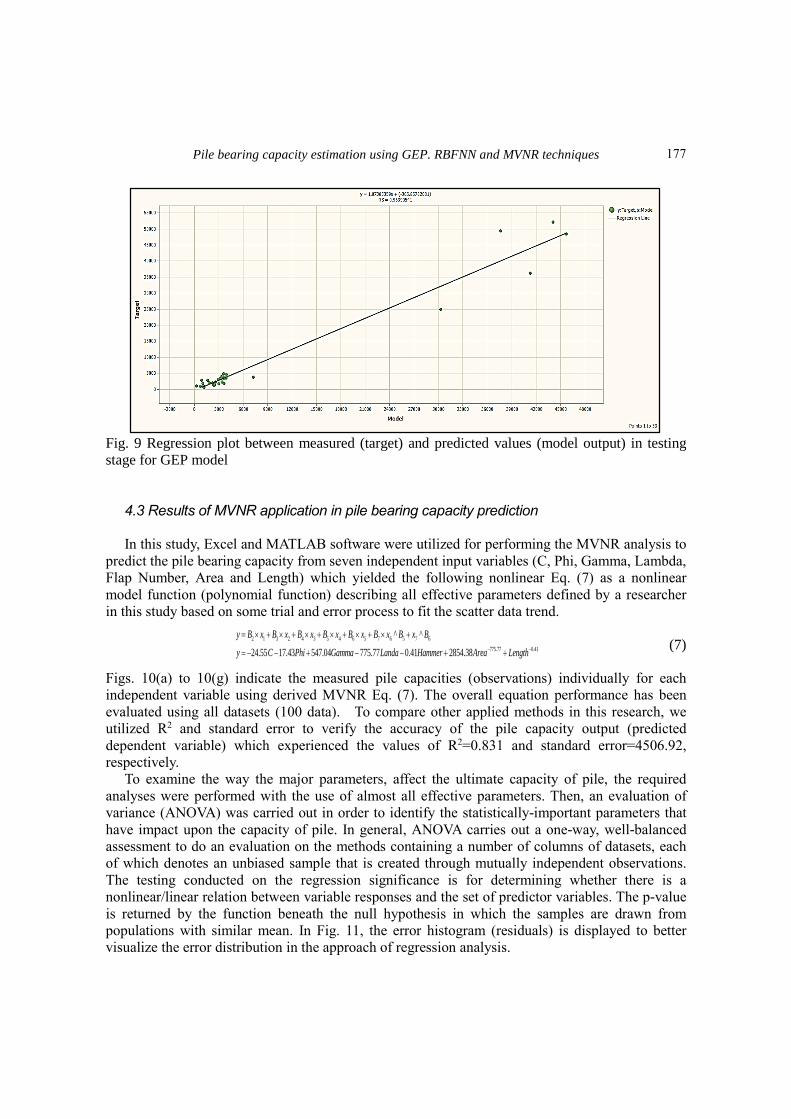
Fig. 9 Regression plot between measured (target) and predicted values (model output) in testing
stage for GEP model
4.3 Results of MVNR application in pile bearing capacity prediction
In this study, Excel and MATLAB software were utilized for performing the MVNR analysis to
predict the pile bearing capacity from seven independent input variables (C, Phi, Gamma, Lambda,
Flap Number, Area and Length) which yielded the following nonlinear Eq. (7) as a nonlinear
model function (polynomial function) describing all effective parameters defined by a researcher
in this study based on some trial and error process to fit the scatter data trend.
(7)
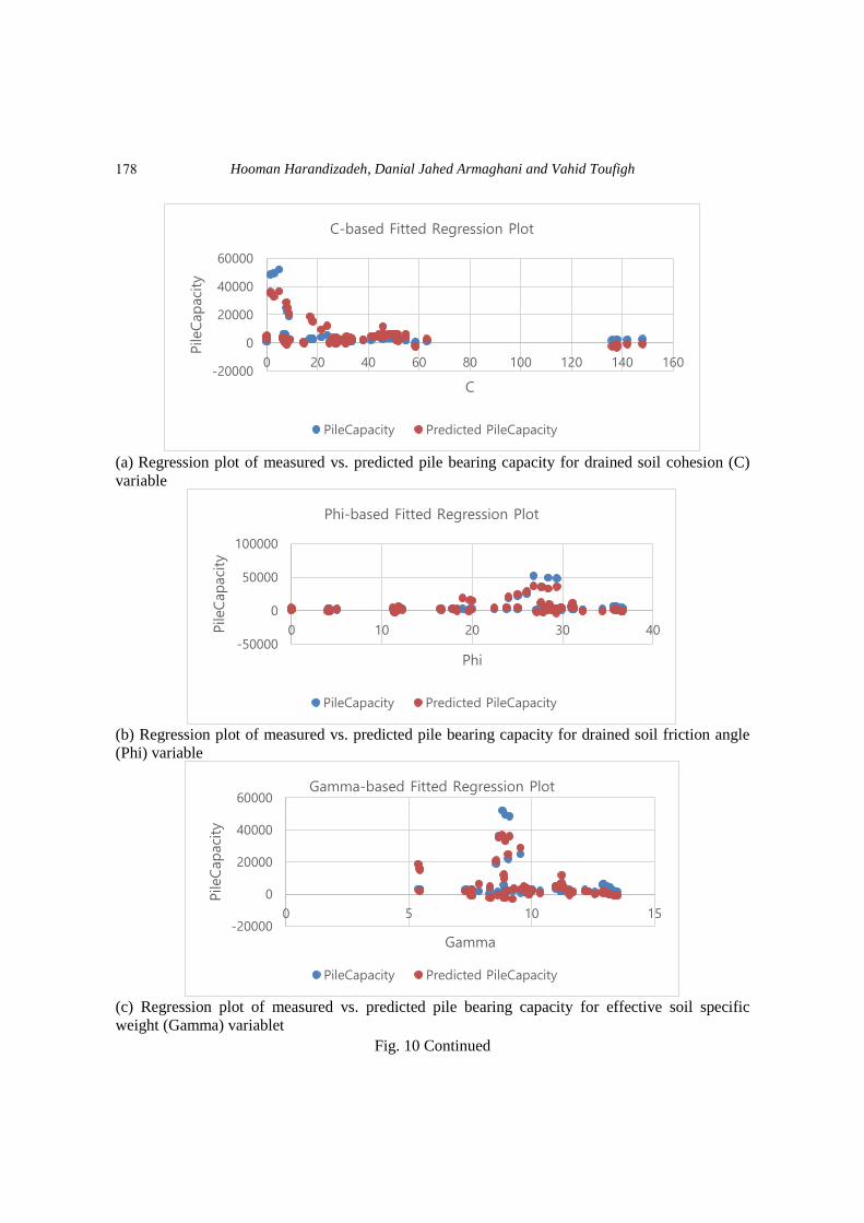
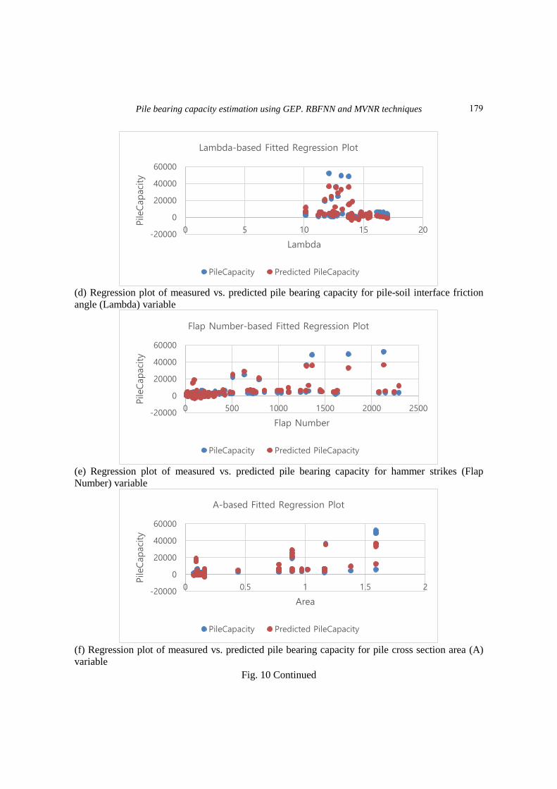
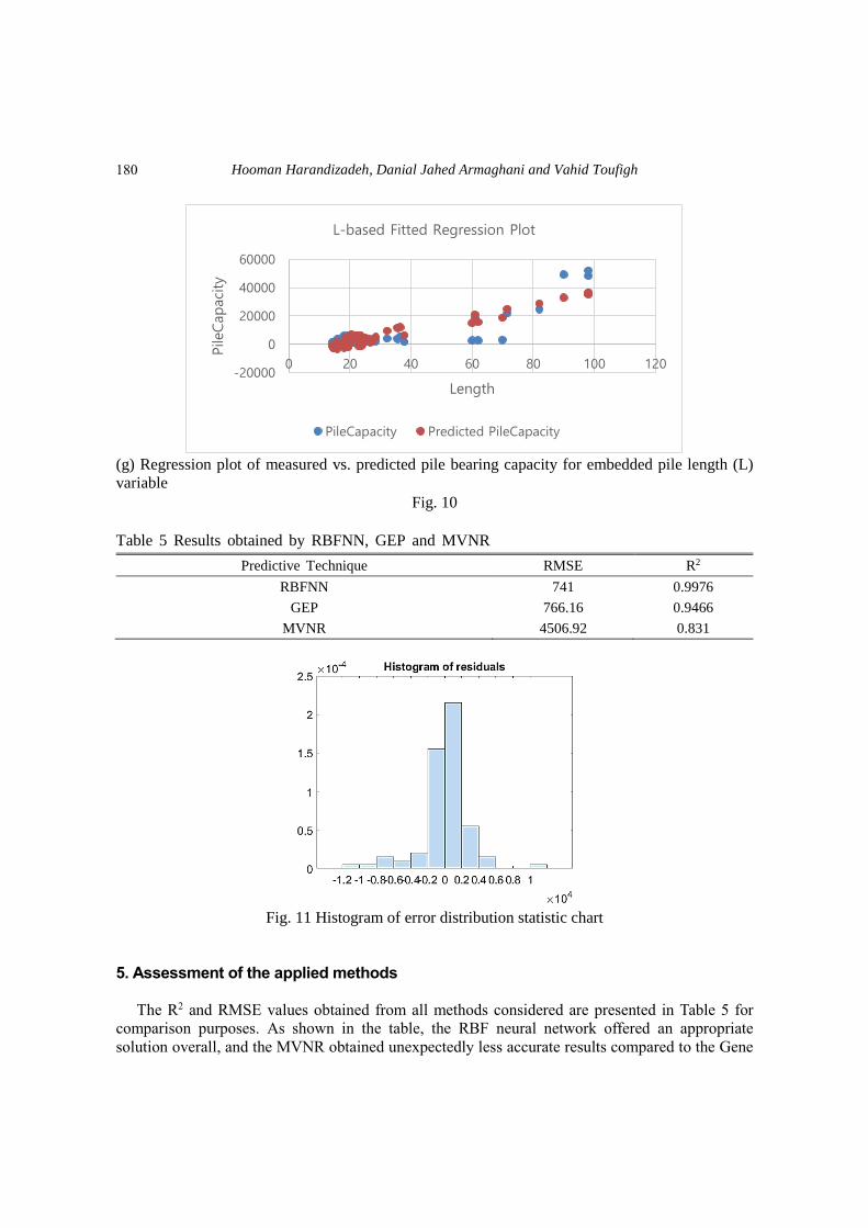
Figs. 10(a) to 10(g) indicate the measured pile capacities (observations) individually for each
independent variable using derived MVNR Eq. (7). The overall equation performance has been
evaluated using all datasets (100 data). To compare other applied methods in this research, we
utilized R2 and standard error to verify the accuracy of the pile capacity output (predicted
dependent variable) which experienced the values of R2=0.831 and standard error=4506.92,
respectively.
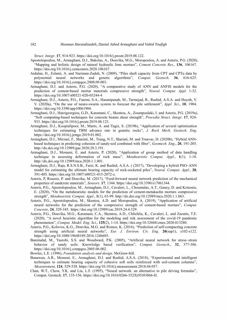
To examine the way the major parameters, affect the ultimate capacity of pile, the required
analyses were performed with the use of almost all effective parameters. Then, an evaluation of
variance (ANOVA) was carried out in order to identify the statistically-important parameters that
have impact upon the capacity of pile. In general, ANOVA carries out a one-way, well-balanced
assessment to do an evaluation on the methods containing a number of columns of datasets, each
of which denotes an unbiased sample that is created through mutually independent observations.
The testing conducted on the regression significance is for determining whether there is a
nonlinear/linear relation between variable responses and the set of predictor variables. The p-value
is returned by the function beneath the null hypothesis in which the samples are drawn from
populations with similar mean. In Fig. 11, the error histogram (residuals) is displayed to better
visualize the error distribution in the approach of regression analysis.
2 1 3 2 4 3 5 4 6 5 7
775
6 5 7 6
0.41.7717.43 547.04 775.77 0.41 2854.
^ ^
24.55 38
y B x B x B x B x B x B x B x B
y C Phi Gamma Landa Hammer Area Length
177
Hooman Harandizadeh, Danial Jahed Armaghani and Vahid Toufigh
(a) Regression plot of measured vs. predicted pile bearing capacity for drained soil cohesion (C)
variable
(b) Regression plot of measured vs. predicted pile bearing capacity for drained soil friction angle
(Phi) variable
(c) Regression plot of measured vs. predicted pile bearing capacity for effective soil specific
weight (Gamma) variablet
Fig. 10 Continued
-20000
0
20000
40000
60000
0 20 40 60 80 100 120 140 160
Pile
Capaci
ty
C
C-based Fitted Regression Plot
PileCapacity Predicted PileCapacity
-50000
0
50000
100000
0 10 20 30 40Pile
Capaci
ty
Phi
Phi-based Fitted Regression Plot
PileCapacity Predicted PileCapacity
-20000
0
20000
40000
60000
0 5 10 15
Pile
Capaci
ty
Gamma
Gamma-based Fitted Regression Plot
PileCapacity Predicted PileCapacity
178
Pile bearing capacity estimation using GEP. RBFNN and MVNR techniques
(d) Regression plot of measured vs. predicted pile bearing capacity for pile-soil interface friction
angle (Lambda) variable
(e) Regression plot of measured vs. predicted pile bearing capacity for hammer strikes (Flap
Number) variable
(f) Regression plot of measured vs. predicted pile bearing capacity for pile cross section area (A)
variable
Fig. 10 Continued
-20000
0
20000
40000
60000
0 5 10 15 20
Pile
Capaci
ty
Lambda
Lambda-based Fitted Regression Plot
PileCapacity Predicted PileCapacity
-20000
0
20000
40000
60000
0 500 1000 1500 2000 2500
Pile
Capaci
ty
Flap Number
Flap Number-based Fitted Regression Plot
PileCapacity Predicted PileCapacity
-20000
0
20000
40000
60000
0 0.5 1 1.5 2
Pile
Capaci
ty
Area
A-based Fitted Regression Plot
PileCapacity Predicted PileCapacity
179
Hooman Harandizadeh, Danial Jahed Armaghani and Vahid Toufigh
(g) Regression plot of measured vs. predicted pile bearing capacity for embedded pile length (L)
variable
Fig. 10
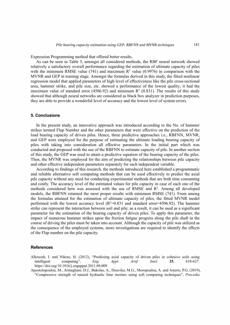
Table 5 Results obtained by RBFNN, GEP and MVNR
Predictive Technique RMSE R2
RBFNN 741 0.9976
GEP 766.16 0.9466
MVNR 4506.92 0.831
Fig. 11 Histogram of error distribution statistic chart
5. Assessment of the applied methods
The R2 and RMSE values obtained from all methods considered are presented in Table 5 for
comparison purposes. As shown in the table, the RBF neural network offered an appropriate
solution overall, and the MVNR obtained unexpectedly less accurate results compared to the Gene
-20000
0
20000
40000
60000
0 20 40 60 80 100 120
Pile
Capaci
ty
Length
L-based Fitted Regression Plot
PileCapacity Predicted PileCapacity
180
Pile bearing capacity estimation using GEP. RBFNN and MVNR techniques
Expression Programming method that offered better results.
As can be seen in Table 5, amongst all considered methods, the RBF neural network showed
relatively a satisfactory overall performance regarding the estimation of ultimate capacity of piles
with the minimum RMSE value (741) and maximum R2 value (0.9976) in comparison with the
MVNR and GEP in training stage. Amongst the formulas derived in this study, the fitted nonlinear
regression model that applied parameters of high level of effectiveness like the pile cross-sectional
area, hammer strike, and pile size, etc. showed a performance of the lowest quality; it had the
maximum value of standard error (4506.92) and minimum R2 (0.831). The results of this study
showed that although neural networks are considered as black box analyzer in prediction purposes,
they are able to provide a wonderful level of accuracy and the lowest level of system errors.
5. Conclusions
In the present study, an innovative approach was introduced according to the No. of hammer
strikes termed Flap Number and the other parameters that were effective on the prediction of the
load bearing capacity of driven piles. Hence, three predictive approaches i.e., RBFNN, MVNR,
and GEP were employed for the purpose of estimating the ultimate loading bearing capacity of
piles with taking into consideration all effective parameters. In the initial part which was
conducted and proposed with the use of the RBFNN to estimate capacity of pile. In another section
of this study, the GEP was used to attain a predictive equation of the bearing capacity of the piles.
Then, the MVNR was employed for the aim of predicting the relationships between pile capacity
and other effective independent parameters separately for each independent variable.
According to findings of this research, the methods introduced here established a programmatic
and reliable alternative soft computing methods that can be used effectively to predict the axial
pile capacity without any need for conducting experimental methods that are both time consuming
and costly. The accuracy level of the estimated values for pile capacity in case of each one of the
methods considered here was assessed with the use of RMSE and R2. Among all developed
models, the RBFNN returned the most proper results with minimum RMSE (741). From among
the formulas attained for the estimation of ultimate capacity of piles, the fitted MVNR model
performed with the lowest accuracy level (R2=0.831 and standard error=4506.92). The hammer
strike can represent the interaction between soil and pile; as a result, it can be used as a significant
parameter for the estimation of the bearing capacity of driven piles. To apply this parameter, the
impact of numerous hammer strikes upon the friction fatigue progress along the pile shaft in the
course of driving the piles must be taken into account. Although the capacity of pile was utilized as
the consequence of the employed systems, more investigations are required to identify the effects
of the Flap number on the pile capacity.
References Alkroosh, I. and Nikraz, H. (2012), “Predicting axial capacity of driven piles in cohesive soils using
intelligent computing”, Eng. Appl. Artif. Intel. 25, 618-627.
https://doi.org/10.1016/j.engappai.2011.08.009
Apostolopoulou, M., Armaghani, D.J., Bakolas, A., Douvika, M.G., Moropoulou, A. and Asteris, P.G. (2019),
“Compressive strength of natural hydraulic lime mortars using soft computing techniques”, Procedia
181
Hooman Harandizadeh, Danial Jahed Armaghani and Vahid Toufigh
Struct. Integr. 17, 914-923. https://doi.org/10.1016/j.prostr.2019.08.122.
Apostolopoulou, M., Armaghani, D.J., Bakolas, A., Douvika, M.G., Moropoulou, A. and Asteris, P.G. (2020),
“Mapping and holistic design of natural hydraulic lime mortars”, Cement Concrete Res., 136, 106167.
https://doi.org/10.1016/j.cemconres.2020.106167.
Ardalan, H., Eslami, A. and Nariman-Zadeh, N. (2009), “Piles shaft capacity from CPT and CPTu data by
polynomial neural networks and genetic algorithms”, Comput. Geotech. 36, 616-625.
https://doi.org/10.1016/j.compgeo.2008.09.003.
Armaghani, D.J. and Asteris, P.G. (2020), “A comparative study of ANN and ANFIS models for the
prediction of cement-based mortar materials compressive strength”, Neural. Comput. Appl. 1-32.
https://doi.org/10.1007/s00521-020-05244-4
Armaghani, D.J., Asteris, P.G., Fatemi, S.A., Hasanipanah, M., Tarinejad, R., Rashid, A.S.A. and Huynh, V.
V. (2020a), “On the use of neuro-swarm system to forecast the pile settlement”, Appl. Sci., 10, 1904.
https://doi.org/10.3390/app10061904.
Armaghani, D.J., Hatzigeorgiou, G.D., Karamani, C., Skentou, A., Zoumpoulaki, I. and Asteris, P.G. (2019a),
“Soft computing-based techniques for concrete beams shear strength”, Procedia Struct. Integr. 17, 924-
933. https://doi.org/10.1016/j.prostr.2019.08.123.
Armaghani, D.J., Koopialipoor, M., Marto, A. and Yagiz, S. (2019b), “Application of several optimization
techniques for estimating TBM advance rate in granitic rocks”, J. Rock Mech. Geotech. Eng.
https://doi.org/10.1016/j.jrmge.2019.01.002.
Armaghani, D.J., Mirzaei, F., Shariati, M., Trung, N.T., Shariati, M. and Trnavac, D. (2020b), “Hybrid ANN-
based techniques in predicting cohesion of sandy-soil combined with fiber”, Geomech. Eng., 20, 191-205.
http://dx.doi.org/10.12989/gae.2020.20.3.191.
Armaghani, D.J., Momeni, E. and Asteris, P. (2020), “Application of group method of data handling
technique in assessing deformation of rock mass”, Metaheuristic Comput. Appl., 1(1), 1-18.
http://dx.doi.org/10.12989/mca.2020.1.1.001.
Armaghani, D.J., Raja, R.S.N.S.B., Faizi, K. and Rashid, A.S.A. ( (2017), “Developing a hybrid PSO–ANN
model for estimating the ultimate bearing capacity of rock-socketed piles”, Neural. Comput. Appl., 28,
391-405. https://doi.org/10.1007/s00521-015-2072-z.
Asteris, P, Roussis, P. and Douvika, M. (2017), “Feed-forward neural network prediction of the mechanical
properties of sandcrete materials”, Sensors. 17, 1344. https://doi.org/10.3390/s17061344.
Asteris, P.G., Apostolopoulou, M., Armaghani, D.J., Cavaleri, L., Chountalas, A.T., Guney, D. and Kotsonis,
E. (2020), “On the metaheuristic models for the prediction of cement-metakaolin mortars compressive
strength”, Metaheuristic Comput. Appl., 1(1), 63-99. http://dx.doi.org/10.12989/mca.2020.1.1.063.
Asteris, P.G., Apostolopoulou, M., Skentou, A.D. and Moropoulou, A. (2019), “Application of artificial
neural networks for the prediction of the compressive strength of cement-based mortars”, Comput.
Concrete, 24, 329-345. https://doi.org/10.12989/cac.2019.24.4.329.
Asteris, P.G., Douvika, M.G., Karamani, C.A., Skentou, A.D., Chlichlia, K., Cavaleri, L. and Zaoutis, T.E.
(2020), “A novel heuristic algorithm for the modeling and risk assessment of the covid-19 pandemic
phenomenon”, Comput. Model. Eng. Sci., 125(2), 1-14. https://doi.org/10.32604/cmes.2020.013280.
Asteris, P.G., Kolovos, K.G., Douvika, M.G. and Roinos, K. (2016), “Prediction of self-compacting concrete
strength using artificial neural networks”, Eur. J. Environ. Civ. Eng. 20(sup1), s102-s122.
https://doi.org/10.1080/19648189.2016.1246693.
Banimahd, M., Yasrobi, S.S. and Woodward, P.K. (2005), “Artificial neural network for stress–strain
behavior of sandy soils: Knowledge based verification”, Comput. Geotech., 32, 377-386.
https://doi.org/10.1016/j.compgeo.2005.06.002.
Bowles, L.E. (1996), Foundation analysis and design. McGraw-hill.
Bunawan, A.R., Momeni, E., Armaghani, D.J. and Rashid, A.S.A. (2018), “Experimental and intelligent
techniques to estimate bearing capacity of cohesive soft soils reinforced with soil-cement columns”,
Measurement, 124, 529-538. https://doi.org/10.1016/j.measurement.2018.04.057.
Chan, W.T., Chow, Y.K. and Liu, L.F. (1995), “Neural network: an alternative to pile driving formulas”,
Comput. Geotech. 17, 135-156. https://doi.org/10.1016/0266-352X(95)93866-H.
182
Pile bearing capacity estimation using GEP. RBFNN and MVNR techniques
Chen, H., Asteris, P.G., Jahed Armaghani, D., Gordan, B. and Pham, B.T. (2019a), “Assessing dynamic
conditions of the retaining wall: Developing two hybrid intelligent models.”, Appl. Sci., 9, 1042.
https://doi.org/10.3390/app9061042.
Chen, W., Sarir, P., Bui, X.N., Nguyen, H., Tahir, M.M. and Armaghani, D.J. (2019b), “Neuro-genetic,
neuro-imperialism and genetic programing models in predicting ultimate bearing capacity of pile”, Eng.
Comput., https://doi.org/10.1007/s00366-019-00752-x.
Das, S.K. and Suman, S. (2015), “Prediction of lateral load capacity of pile in clay using multivariate
adaptive regression spline and functional network”, Arab. J. Sci. Eng., 40, 1565-1578. https://doi.org/10.1007/s13369-015-1624-y.
Duan, J., Asteris, P.G., Nguyen, H., Bui, X.N. and Moayedi, H. (2020), “A novel artificial intelligence
technique to predict compressive strength of recycled aggregate concrete using ICA-XGBoost model”,
Eng. Comput. https://doi.org/10.1007/s00366-020-01003-0.
Erzin, Y., Rao, B.H. and Singh, D.N. (2008), “Artificial neural network models for predicting soil thermal
resistivity”, Int. J. Therm. Sci., 47, 1347-1358. https://doi.org/10.1016/j.ijthermalsci.2007.11.001.
Eslami, A. (1996), Bearing capacity of piles from cone penetration data.
Hajihassani, M., Abdullah, S.S., Asteris, P.G. and Armaghani, D.J. (2019), “A gene expression programming
model for predicting tunnel convergence”, Appl. Sci., 9, 4650. https://doi.org/10.3390/app9214650.
Hansen, J.B. (1963), “Discussion on hyperbolic stress-strain response: Cohesive soils”, J. Soil Mech. Found.
Eng., 89(4), 241-242
Harandizadeh, H., Armaghani, D.J. and Khari, M. (2019a), “A new development of ANFIS–GMDH
optimized by PSO to predict pile bearing capacity based on experimental datasets”, Eng. Comput. 1-16.
https://doi.org/10.1007/s00366-019-00849-3
Harandizadeh, H., Toufigh, M.M. and Toufigh, V. (2018), “Different neural networks and modal tree method
for predicting ultimate bearing capacity of piles”, Iran Univ. Sci. Technol., 8, 311-328.
http://ijoce.iust.ac.ir/article-1-347-en.html.
Harandizadeh, H., Toufigh, M.M. and Toufigh, V. (2019b), “Application of improved ANFIS approaches to
estimate bearing capacity of piles”, Soft Comput., 23(19), 9537-9549. https://doi.org/10.1007/s00500-018-
3517-y.
Huang, L., Asteris, P.G., Koopialipoor, M., Armaghani, D.J. and Tahir, M.M. (2019), “Invasive weed
optimization technique-based ANN to the prediction of rock tensile strength”, Appl. Sci., 9(24), 5372.
https://doi.org/10.3390/app9245372.
Javadi, A.A., Rezania, M. and Nezhad, M.M. (2006), “Evaluation of liquefaction induced lateral
displacements using genetic programming”, Comput. Geotech., 33, 222-233.
https://doi.org/10.1016/j.compgeo.2006.05.001.
Kayadelen, C. (2011), “Soil liquefaction modeling by genetic expression programming and neuro-fuzzy”,
Expert Syst. Appl., 38(4), 4080-4087. https://doi.org/10.1016/j.eswa.2010.09.071.
Kechagias, J., Tsiolikas, A., Asteris, P. and Vaxevanidis, N. (2018), “Optimizing ANN performance using
DOE: application on turning of a titanium alloy”, In: MATEC Web of Conferences. EDP Sciences.
Khari, M., Armaghani, D.J. and Dehghanbanadaki, A. (2019a), “Prediction of lateral deflection of small-
scale piles using hybrid PSO–ANN model.”, 1-11. Arab. J. Sci. Eng., https://doi.org/10.1007/s13369-019-
04134-9
Khari, M., Dehghanbandaki, A., Motamedi, S. and Armaghani, D.J. (2019b), “Computational estimation of
lateral pile displacement in layered sand using experimental data”, Measurement, 146, 110-118.
https://doi.org/10.1016/j.measurement.2019.04.081.
Kiefa, M.A.A. (1998), “General regression neural networks for driven piles in cohesionless soils”, J.
Geotech. Geoenvironm. Eng., 124(12), 1177-1185. https://doi.org/10.1061/(ASCE)1090-
0241(1998)124:12(1177).
Koopialipoor, M., Nikouei, S.S., Marto, A., Fahimifar, A., Armaghani, D.J. and Mohamad, E.T. (2018),
“Predicting tunnel boring machine performance through a new model based on the group method of data
handling”, Bull. Eng. Geol. Environ. 78, 3799-3813. https://doi.org/10.1007/s10064-018-1349-8.
Koza, J.R. (1992), Genetic programming II. automatic discovery of reusable subprograms, MIT Press,
183
Hooman Harandizadeh, Danial Jahed Armaghani and Vahid Toufigh
Cambridge, M.A.
Kurup, P.U. and Griffin, E.P. (2006), “Prediction of soil composition from CPT data using general regression
neural network”, J. Comput. Civil Eng., 20, 281-289. https://doi.org/10.1061/(ASCE)0887-
3801(2006)20:4(281).
Lee, I.M. and Lee, J.H. (1996), “Prediction of pile bearing capacity using artificial neural networks”,
Comput. Geotech., 18, 189-200. https://doi.org/10.1016/0266-352X(95)00027-8.
Lu, S., Koopialipoor, M., Asteris, P.G., Bahri, M. and Armaghani, D.J. (2020), “A novel feature selection
approach based on tree models for evaluating the punching shear capacity of steel fiber-reinforced
concrete flat slabs”, Materials (Basel). 13, 3902. https://doi.org/10.3390/ma13173902.
Meschke, G., Ninić, J., Stascheit, J. and Alsahly, A. (2013), “Parallelized computational modeling of pile-
soil interactions in mechanized tunneling”, Eng. Struct., 47, 35-44.
https://doi.org/10.1016/j.engstruct.2012.07.001.
Milad, F., Kamal, T., Nader, H. and Erman, O.E. (2015), “New method for predicting the ultimate bearing
capacity of driven piles by using Flap number”, KSCE J. Civil Eng., 19, 611-620. https://doi.org/10.1007/s12205-013-0315-z.
Moayedi, H. and Armaghani, D.J. (2018), “Optimizing an ANN model with ICA for estimating bearing
capacity of driven pile in cohesionless soil”, Eng. Comput., 34, 347-356. https://doi.org/10.1007/s00366-
017-0545-7.
Momeni, E. Armaghani, D.J. Fatemi, S.A. and Nazir, R. (2018), “Prediction of bearing capacity of thin-
walled foundation: a simulation approach”, Eng. Comput., 34, 319-327. https://doi.org/10.1007/s00366-
017-0542-x.
Momeni, E., Dowlatshahi, M.B., Omidinasab, F., Maizir, H. and Armaghani, D.J. (2020), “Gaussian process
regression technique to estimate the pile bearing capacity”, Arab. J. Sci. Eng.,
https://doi.org/10.1007/s13369-020-04683-4.
Momeni, E., Maizir, H., Gofar, N. and Nazir, R. (2013), “Comparative study on prediction of axial bearing
capacity of driven piles in granular materials”, J. Teknol., 61(3), 15-20.
Momeni, E., Nazir, R., Armaghani, D.J. and Maizir, H. (2014), “Prediction of pile bearing capacity using a
hybrid genetic algorithm-based ANN”, Measurement, 57, 122-131.
https://doi.org/10.1016/j.measurement.2014.08.007.
Momeni, E., Nazir, R., Armaghani, D.J. and Maizir, H. (2015a), “Application of artificial neural network for
predicting shaft and tip resistances of concrete piles”, Earth Sci. Res. J., 19, 85-93.
http://dx.doi.org/10.15446/esrj.v19n1.38712.
Momeni, E., Nazir, R., Armaghani, D.J. and Sohaie, H. (2015b), “Bearing capacity of precast thin-walled
foundation in sand”, Proc. Institution Civil Eng. Geotech. Eng., 168, 539-550.
https://doi.org/10.1680/jgeen.14.00177.
Najafzadeh, M. (2015), “Neuro-fuzzy GMDH systems based evolutionary algorithms to predict scour pile
groups in clear water conditions”, Ocean Eng., 99, 85-94. https://doi.org/10.1016/j.oceaneng.2015.01.014.
Najafzadeh, M. and Azamathulla, H.M. (2013), “Neuro-fuzzy GMDH to predict the scour pile groups due to
waves”, J. Comput. Civil Eng., 29, 4014068. https://doi.org/10.1061/(ASCE)CP.1943-5487.0000376.
Najafzadeh, M. and Bonakdari, H. (2016), “Application of a neuro-fuzzy GMDH model for predicting the
velocity at limit of deposition in storm sewers”, J. Pipeline Syst. Eng. Pract., 8:6016003.
https://doi.org/10.1061/(ASCE)PS.1949-1204.0000249.
Najafzadeh, M. Barani, G.A. and Azamathulla, H.M. (2013), “GMDH to predict scour depth around a pier in
cohesive soils”, Appl. Ocean Res., 40, 35-41. https://doi.org/10.1016/j.apor.2012.12.004.
Prakash, S. and Sharma, H.D. (1990), Pile foundations in engineering practice, John Wiley & Sons
Samui, P. (2008), “Prediction of friction capacity of driven piles in clay using the support vector machine”,
Can. Geotech. J., 45, 288-295. https://doi.org/10.1139/T07-072.
Samui, P. (2012), “Determination of ultimate capacity of driven piles in cohesionless soil: A multivariate
adaptive regression spline approach”, Int. J. Numer. Analy. Meth. Geomech., 36(11), 1434-1439.
https://doi.org/10.1007/s00521-012-1043-x.
Samui, P. and Kim, D. (2013), “Least square support vector machine and multivariate adaptive regression
184
Pile bearing capacity estimation using GEP. RBFNN and MVNR techniques
spline for modeling lateral load capacity of piles”, Neural Comput. Appl., 23, 1123-1127.
https://doi.org/10.1007/s00366-019-00808-y.
Sarir, P., Chen, J., Asteris, P.G., Armaghani, D.J. and Tahir, M.M. (2019), “Developing GEP tree-based,
neuro-swarm, and whale optimization models for evaluation of bearing capacity of concrete-filled steel
tube columns”, Eng. Comput., 1-19. https://doi.org/10.1007/s00366-019-00808-y.
Sette, S. and Boullart, L. (2001), “Genetic programming: principles and applications”, Eng. Appl. Artif.
Intell., 14, 727-736. https://doi.org/10.1016/S0952-1976(02)00013-1.
Shahin, M.A., Maier, H.R. and Jaksa, M.B. (2002), “Predicting settlement of shallow foundations using
neural networks”, J. Geotech. Geoenviron. Eng., 128, 785-793. https://doi.org/10.1061/(ASCE)1090-
0241(2002)128:9(785).
Sinha, S.K. and Wang, M.C. (2008), “Artificial neural network prediction models for soil compaction and
permeability”, Geotech. Geol. Eng., 26, 47-64. https://doi.org/10.1007/s10706-007-9146-3.
Toghroli, A., Mohammadhassani, M., Suhatril, M., Shariati, M. and Ibrahim, Z. (2014), “Prediction of shear
capacity of channel shear connectors using the ANFIS model”, Steel Compos. Struct., 17, 623-639.
http://dx.doi.org/10.12989/scs.2014.17.5.623.
Tomlinson, M. and Woodward, J. (2007), Pile design and construction practice. Crc Press
Wang, M. Shi, X., Zhou, J. and Qiu, X. (2018), “Multi-planar detection optimization algorithm for the
interval charging structure of large-diameter longhole blasting design based on rock fragmentation
aspects”, Eng. Optim., 50, 2177-2191. https://doi.org/10.1080/0305215X.2018.1439943.
Wu, Y., Zhang, K., Fu, L., Liu, J. and He, J. (2019), “Performance of cement–soil pile composite foundation
with lateral constraint”, Arab. J. Sci. Eng., 44, 4693-4702. https://doi.org/10.1007/s13369-018-3519-1.
Xu, C., Gordan, B., Koopialipoor, M., Armaghani, D.J., Tahir, M.M. and Zhang, X. (2019a), “Improving
performance of retaining walls under dynamic conditions developing an optimized ANN based on ant
colony optimization technique”, IEEE Access. 7, 94692-94700.
https://doi.org/10.1109/ACCESS.2019.2927632.
Xu, H., Zhou, J., G Asteris, P., Jahed Armaghani, D. and Tahir, M.M. (2019b), “Supervised machine learning
techniques to the prediction of tunnel boring machine penetration rate”, Appl. Sci., 9, 3715.
https://doi.org/10.3390/app9183715.
Yang H, Liu J, Liu B (2018) Investigation on the cracking character of jointed rock mass beneath TBM disc
cutter. Rock Mech Rock Eng 51:1263–1277. https://doi.org/10.1007/s00603-017-1395-8.
Yang H, Wang H, Zhou X (2016) Analysis on the damage behavior of mixed ground during TBM cutting
process. Tunn Undergr Sp Technol 57:55–65. https://doi.org/10.1016/j.tust.2016.02.014.
Yang, H.Q., Zeng, Y.Y., Lan, Y.F. and Zhou, X.P. (2014), “Analysis of the excavation damaged zone around
a tunnel accounting for geostress and unloading”, Int. J. Rock Mech. Min. Sci., 69, 59-66.
https://doi.org/10.1016/j.ijrmms.2014.03.003.
Young-Su K. and Byung-Tak, K. (2006), “Use of artificial neural networks in the prediction of liquefaction
resistance of sands”, J. Geotech. Geoenviron. Eng., 132, 1502-1504. https://doi.org/10.1061/(ASCE)1090-
0241(2006)132:11(1502).
Zhang, W., Wu, C., Li, Y., Wang, L. and Samui, P. (2019), “Assessment of pile drivability using random
forest regression and multivariate adaptive regression splines”, Georisk Assess. Manag. Risk Eng. Syst.
Geohazards. 1-14. https://doi.org/10.1080/17499518.2019.1674340.
Zhou, J., Asteris, P.G., Armaghani, D.J. and Pham, B.T. (2020a), “Prediction of ground vibration induced by
blasting operations through the use of the Bayesian Network and random forest models”, Soil Dyn. Earthq.
Eng., 139, 106390. https://doi.org/10.1016/j.soildyn.2020.106390.
Zhou, J., Li, C., Koopialipoor, M., Jahed Armaghani, D. and Thai Pham, B. (2020b), “Development of a new
methodology for estimating the amount of PPV in surface mines based on prediction and probabilistic
models (GEP-MC)”, Int. J. Min. Reclam. Environ., 35(1), 48-
68.https://doi.org/10.1080/17480930.2020.1734151.
Zhou, J., Li, E., Yang, S., Wang, M., Shi, X., Yao, S. and Mitri, H.S. (2019), “Slope stability prediction for
circular mode failure using gradient boosting machine approach based on an updated database of case
histories”, Saf. Sci., 118, 505-518. https://doi.org/10.1016/j.ssci.2019.05.046.
185
Hooman Harandizadeh, Danial Jahed Armaghani and Vahid Toufigh
Zhou, J., Qiu, Y., Armaghani, D.J., Zhang, W., Li, C., Zhu, S. and Tarinejad, R. (2020c), “Predicting TBM
penetration rate in hard rock condition: A comparative study among six XGB-based metaheuristic
techniques”, Geosci. Front., https://doi.org/10.1016/j.gsf.2020.09.020
Zhou, J., Shi, X., Du, K., Qiu, X., Li, X. and Mitri, H.S. (2016), “Feasibility of random-forest approach for
prediction of ground settlements induced by the construction of a shield-driven tunnel”, Int. J. Geomech.,
17(6), 4016129. https://doi.org/10.1061/(ASCE)GM.1943-5622.0000817.
PA
186
Related Documents