K I P FOR POTSDAM INSTITUTE CLIMATE IMPACT RESEARCH (PIK) PIK Report No. 103 No. 103 Nicola Botta, Cezar Ionescu, Ciaron Linstead, Rupert Klein STRUCTURING DISTRIBUTED RELATION-BASED COMPUTATIONS WITH SCDRC

Welcome message from author
This document is posted to help you gain knowledge. Please leave a comment to let me know what you think about it! Share it to your friends and learn new things together.
Transcript
KIP
FOR
POTSDAM INSTITUTE
CLIMATE IMPACT RESEARCH (PIK)
PIK Report
No. 103No. 103
Nicola Botta, Cezar Ionescu, Ciaron Linstead, Rupert Klein
STRUCTURING DISTRIBUTEDRELATION-BASED COMPUTATIONS WITH
SCDRC

Herausgeber:Prof. Dr. F.-W. Gerstengarbe
Technische Ausführung:U. Werner
POTSDAM-INSTITUTFÜR KLIMAFOLGENFORSCHUNGTelegrafenbergPostfach 60 12 03, 14412 PotsdamGERMANYTel.: +49 (331) 288-2500Fax: +49 (331) 288-2600E-mail-Adresse:[email protected]
Corresponding author:Dr. Nicola BottaPotsdam Institute for Climate Impact ResearchP.O. Box 60 12 03, D-14412 Potsdam, GermanyPhone: +49-331-288-2657Fax: +49-331-288-2695E-mail: [email protected]
POTSDAM, OKTOBER 2006ISSN 1436-0179
STRUCTURING DISTRIBUTED RELATION-BASED COMPUTATIONS WITH SCDRC 3
Abstract
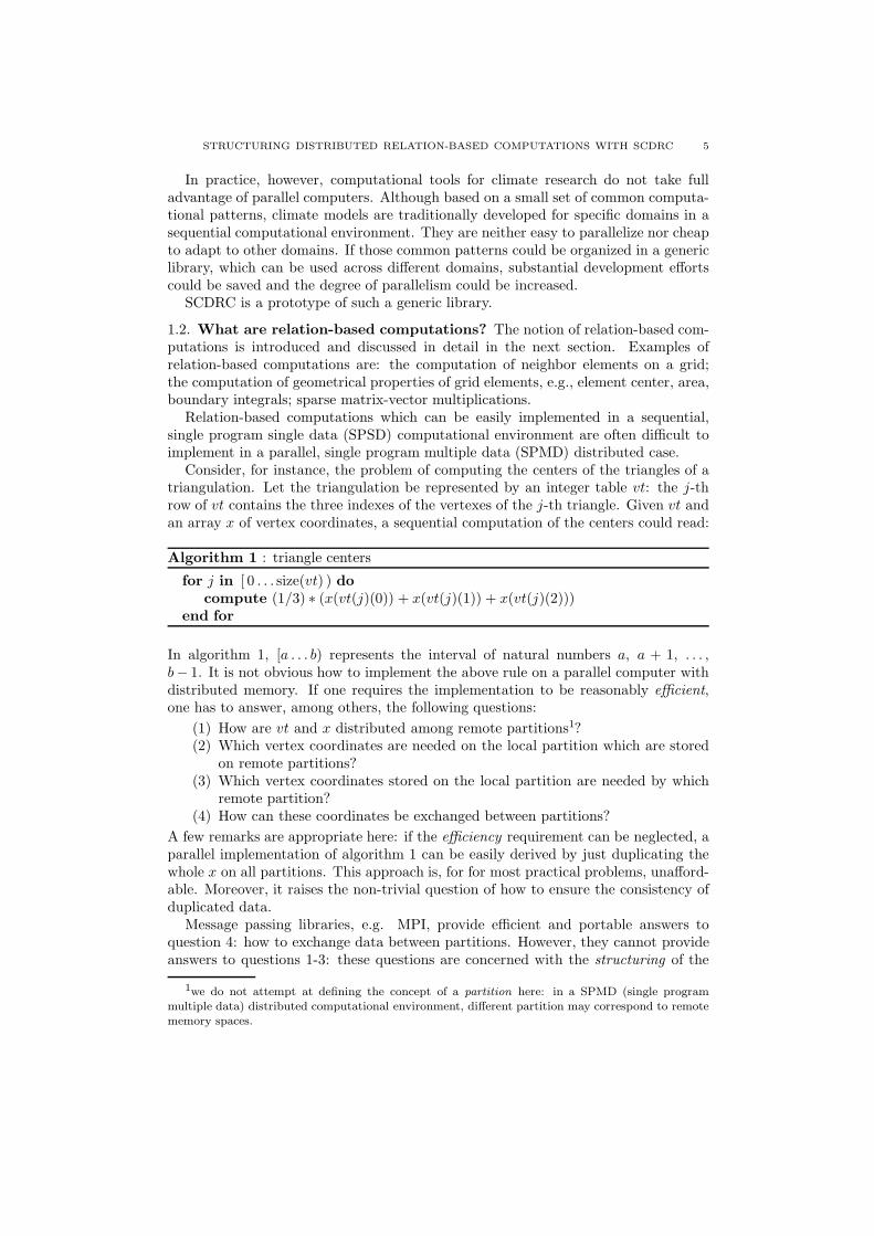
In this report we present a set of software components for distributed relation-basedcomputations (SCDRC).We explain how SCDRC can be used to structure parallelcomputations in a single-program multiple-data computational environment.
First, we introduce relation-based algorithms and relation-based computations asgeneric patterns in scientific computing. We then discuss the problems that have tobe solved to parallelize such patterns and propose a high-level formalism for specifyingthese problems.
This formalism is then applied to derive parallel distributed relation-based com-putations. These are implemented in the C++ library SCDRC. We present languageindependent elements of SCDRC and discuss C++ specific aspects of its design andarchitecture.
Finally, we discuss how to use SCDRC in a simple application and provide prelim-inary performance figures.

4 N. BOTTA, C. IONESCU, C. LINSTEAD, R. KLEIN
Contents
Abstract 31. Introduction 41.1. What is SCDRC? 41.2. What are relation-based computations? 51.3. Who can take advantage from SCDRC? 61.4. How does SCDRC compare to other approaches? 61.5. What is the state of development of SCDRC? 81.6. Outline 82. Relation-based algorithms and relation-based computations 82.1. Relation-based algorithms 82.2. Relation-based computations 112.3. Core problems 123. Implementation independent elements 133.1. Set, function and relation representations 133.2. Distributed functions and distributed relations 143.3. Problem specification 164. Implementation dependent elements 294.1. Computational environments and namespaces 294.2. Components, files, directories 344.3. Interfaces, class operations, contracts and documentation 364.4. Iterators 404.5. Relations 414.6. Relation-based algorithms 434.7. Communication primitives, exchange and MPI interface 445. Preliminary results, outlook 455.1. Center of area computations 455.2. Preliminary results 505.3. Outlook 55Acknowledgements 55References 55
1. Introduction
1.1. What is SCDRC? SCDRC is a set of software components for structuringdistributed relation-based computations.
Relation-based computations are simple but general patterns found in many sci-entific computing domains. In climate research, they are at the core of grid-basednumerical methods for partial differential equations (ocean and atmosphere models),of inference algorithms for Bayesian networks and of viability kernel algorithms (vi-ability studies). They also arise in data interpolation between regular and irregulargrids (pre-processing, model coupling).
Relation-based computations are often nested in expensive, iterative programs.These programs could, in principle, take advantage of distributed parallel architec-tures to speed up computations.
In climate research, faster computations allow simulations on longer time scales,improved resolution and more representative sets of realizations in uncertainty studies.
STRUCTURING DISTRIBUTED RELATION-BASED COMPUTATIONS WITH SCDRC 5
In practice, however, computational tools for climate research do not take fulladvantage of parallel computers. Although based on a small set of common computa-tional patterns, climate models are traditionally developed for specific domains in asequential computational environment. They are neither easy to parallelize nor cheapto adapt to other domains. If those common patterns could be organized in a genericlibrary, which can be used across different domains, substantial development effortscould be saved and the degree of parallelism could be increased.
SCDRC is a prototype of such a generic library.
1.2. What are relation-based computations? The notion of relation-based com-putations is introduced and discussed in detail in the next section. Examples ofrelation-based computations are: the computation of neighbor elements on a grid;the computation of geometrical properties of grid elements, e.g., element center, area,boundary integrals; sparse matrix-vector multiplications.
Relation-based computations which can be easily implemented in a sequential,single program single data (SPSD) computational environment are often difficult toimplement in a parallel, single program multiple data (SPMD) distributed case.
Consider, for instance, the problem of computing the centers of the triangles of atriangulation. Let the triangulation be represented by an integer table vt: the j-throw of vt contains the three indexes of the vertexes of the j-th triangle. Given vt andan array x of vertex coordinates, a sequential computation of the centers could read:
Algorithm 1 : triangle centers
for j in [ 0 . . . size(vt) ) do
compute (1/3) ∗ (x(vt(j)(0)) + x(vt(j)(1)) + x(vt(j)(2)))end for
In algorithm 1, [a . . . b) represents the interval of natural numbers a, a + 1, . . . ,b− 1. It is not obvious how to implement the above rule on a parallel computer withdistributed memory. If one requires the implementation to be reasonably efficient,one has to answer, among others, the following questions:
(1) How are vt and x distributed among remote partitions1?(2) Which vertex coordinates are needed on the local partition which are stored
on remote partitions?(3) Which vertex coordinates stored on the local partition are needed by which
remote partition?(4) How can these coordinates be exchanged between partitions?
A few remarks are appropriate here: if the efficiency requirement can be neglected, aparallel implementation of algorithm 1 can be easily derived by just duplicating thewhole x on all partitions. This approach is, for for most practical problems, unafford-able. Moreover, it raises the non-trivial question of how to ensure the consistency ofduplicated data.
Message passing libraries, e.g. MPI, provide efficient and portable answers toquestion 4: how to exchange data between partitions. However, they cannot provideanswers to questions 1-3: these questions are concerned with the structuring of the
1we do not attempt at defining the concept of a partition here: in a SPMD (single programmultiple data) distributed computational environment, different partition may correspond to remotememory spaces.

6 N. BOTTA, C. IONESCU, C. LINSTEAD, R. KLEIN
parallel computation. In particular, the answers to question 2 and 3 essentially dependon how question 1 is answered.
Of course, structuring rules or guidelines cannot be given in general but only forcertain classes of computations or computational patterns. Relation-based computa-tions are a family of such patterns.
1.3. Who can take advantage from SCDRC? As a set of components for struc-turing distributed relation-based computations, SCDRC is a software layer abovemessage passing libraries but below applications. It is not meant to be directly usedby application developers. Instead, SCDRC is designed to be the basis on which ap-plication dependent software components are written. In other words, applicationsare expected to use SCDRC indirectly via application dependent abstractions.
As an example, consider a triangulation class supporting the implementation offinite element discrete differential operators. This is an application dependent ab-straction (in the sense that it will implement, among others, methods which arespecific to finite element computations) which could be written on top of SCDRC. Afinite element program for approximating incompressible flows is an example of anapplication.
Being a low-level software layer (w.r.t. applications), SCDRC does not attemptat hiding the communication steps which are needed in relation-based computations.Communication steps which are conceptually complementary but distinct are repre-sented by distinct data structures or function calls.
This means that developers have a high degree of control over communication andcan take advantage of such control for optimizations. However, communication isstructured in a set of primitives which have been specifically designed for relation-based computations. In particular, SCDRC users do not have direct access to standardmessage passing (MPI) primitives and do not need to care about synchronization,mutual exclusion, deadlock or race condition problems. They can develop applicationdependent software components on the top of SCDRC which hide communication orleave it visible to the user.
1.4. How does SCDRC compare to other approaches? A discussion of themany and different approaches towards introducing abstraction layers between mes-sage passing libraries and scientific computing applications goes beyond the scope ofthis report.
For an overview of the role of subroutine libraries and of frameworks in generic soft-ware components for scientific computing we refer the reader to [4]. A comprehensivediscussion of domain specific languages, frameworks and toolkits from the point ofview of domain engineering can be found in [9]. The concepts of grid and of algo-
rithm oriented design of software components for grids and geometries are discussedin [1], [3] and [5].
SCDRC has been designed around patterns which are found in numerical methodsfor partial differential equations (PDE) and in other applications domain: adaptivestochastic sequential decision processes and Bayesian network inference are two promi-nent examples. Up to now, the most significant efforts towards developing frameworksof generic, reusable software components have been done in the PDE application do-main. In the following, we point out differences and similarities between SCDRC andwell established frameworks for solving PDEs.

STRUCTURING DISTRIBUTED RELATION-BASED COMPUTATIONS WITH SCDRC 7
A very elementary difference between SCDRC and frameworks like POOMA2,Overture3, Amatos4 and OpenFoam5 is in terms of size. SCDRC is a very small,thin software layer: at the present stage, sloccount6 counts about 12000 source linesof code in the main directory tree of SCDRC. As a comparison, OpenFoam version1.2 consists of about one million lines of code!
Another important difference between SCDRC and computational frameworks forPDE lies in the level of abstraction. The central concepts in SCDRC are relationsand relation-based computations. The main problems addressed by SCDRC are howto represent distributed relations and how to implement parallel relation-based com-putations.
In numerical frameworks for PDEs, grid concepts play an outstanding role. Gridsare much more complex concepts than relations. One can think of relations in a cou-ple of different ways – as sets of pairs, as characteristic functions or as functions – andone can distinguish between different kinds of relations: regular relations, irregularrelations, etc. This complexity, however, is very little when compared to the com-plexity of grid concepts. The grids needed in computational frameworks for PDEshave geometrical and topological aspects. The latter are described by a whole set ofgrid relations. Grid representations depend on the choice of a coordinate system, onthe number of dimensions of the geometrical space in which they are embedded, on anumber of grid coordinates. One can distinguish between structured and unstructured
grids, between regular and irregular grids, between rectangular, skew and curvilinear
grids. Adaptive grids, hierarchical grids, overlapping and non-overlapping grids areother aspects of different grid taxonomies.
The development of SCDRC is an attempt at tackling the problem of structuringalgorithm-oriented parallel computations on the basis of the smallest common con-cept and of the simplest computational patterns found in a wide class of scientificcomputing problems: relations and relation-based computations.
Since it tackles the parallelization problem at an elementary level, the SCDRCapproach is more similar to the algorithmic skeletons or to POOMA’s stencil -basedapproach than to grid-based domain decomposition approache. As it will become clearin the following sections, relation-based algorithms and relation-based computationsare, in fact, non-trivially parallelizable data parallel algorithmic skeletons in the senseof [14].
Special kind of relations – symmetric, anti-reflexive graphs – play a fundamentalrole in graph partitioning algorithms such as those implemented in the Metis [12]and ParMetis [8] library. As we will see in the next section, SCDRC provide aninterface to these libraries. The interface allows one to apply partitioning algorithmsto SCDRC relations. The application domains of Metis and ParMetis – graph andgrid partitioning – on the one side and of SCDRC on the other side are complementarybut clearly separated.
As a set of software components for structuring distributed relation-based compu-tations, SCDRC provides a subset of the functionalities provided by the Janus frame-work, see [10]. In fact, the initial phase of the SCDRC development has been donein collaboration with Dr. J. Gerlach, the main developer of Janus. As we will show
2http://acts.nersc.gov/pooma3http://acts.nersc.gov/overture4http://www.amatos.info5http://www.opencfd.co.uk/openfoam6By David A. Wheeler, http://www.dwheeler.com/sloccount
8 N. BOTTA, C. IONESCU, C. LINSTEAD, R. KLEIN
in section 3, SCDRC shares with Janus (and with ParMetis) the conceptual modelof representing distributed functions and relations. There are, however, importantdifferences between SCDRC and Janus. These differences are both in implementationindependent aspects and in the implementation design.
A major implementation independent difference is architectural. In contrast toJanus, the architecture of SCDRC is based on the formal specification of a small setof problems. These problems are informally introduced at the end of the next sectionand problem specifications are discussed in detail in section 3.
Another difference between SCDRC and Janus is in how solution algorithms forthe problem specifications of section 3 have been derived. In SCDRC, this has beendone on the basis of a single communication primitive in the spirit of the BSP (bulksynchronous parallel processing) model, see [7], [6]. This communication primitiveis discussed in detail in 3 and 4. In contrast to SCDRC, Janus algorithms are notexplicitly designed around a single communication primitive, and attempt to hide thedistinction between parallel and sequential execution.
A third major difference between Janus and SCDRC is in the approach towardsconstructing relations. Janus supports incremental construction with a very flexible(albeit non trivial) two-phase model. SCDRC takes a more straightforward approachand does not support incremental construction.
1.5. What is the state of development of SCDRC? SCDRC is in a prototypi-cal stage. Its sources are available under the GPL licence but have not been released(please contact [email protected]). SCDRC has been compiled with gcc ver-sion 3.3.6 and 4.0.2 and tested on a linux-cluster under lam-mpi and mpich and ona 240 CPU IBM p655 cluster. At the present, no application dependent softwarecomponents have been built on the top of SCDRC but a few simple examples areprovided.
1.6. Outline. The rest of this report is organized as follows. In section 2 we intro-duce and discuss relation-based algorithms and relation-based computations followingthe triangle center example outlined above. Section 3 describes implementation in-dependent design elements of SCDRC. In this section we discuss, among others, howdistributed functions and distributed relations are conceptually represented – remem-ber question 1) above – and which aspects of this representation are visible to SCDRCusers. In section 4 we discuss implementation dependent aspects and architecture ofSCDRC. In the last section we comment a simple application and discuss preliminaryresults.
2. Relation-based algorithms and relation-based computations
2.1. Relation-based algorithms. Let’s go back to algorithm 1 introduced in section1 to represent a triangle center computation. In this rule we have used x(i) (for iequal to vt(j)(0), vt(j)(1) and vt(j)(0)) to represent the i-th element of the array x.
We use the notation x(i) — in contrast to the more usual x[i] — to underline thefact that, for the purpose of expressing the triangle center computation, the way thevertex coordinates are obtained is immaterial. In concrete implementations, x doesnot need to be an array and one can easily think of triangulations in which the vertexcoordinates are given by analytical expressions.
Let’s take a critical view at algorithm 1: what if the triangulation covers a sphereand the triangles themselves are spherical? In this case, algorithm 1 yields triangle

STRUCTURING DISTRIBUTED RELATION-BASED COMPUTATIONS WITH SCDRC 9
centers that do not lie on the surface of the sphere. This is probably not what atriangle centers algorithm is meant to compute. Algorithm 1 can be easily modifiedto avoid triangle shape over-specification:
Algorithm 2 : triangle centers
for j in [ 0 . . . size(vt) ) do
compute center(x(vt(j)(0)), x(vt(j)(1)), x(vt(j)(2)))end for
The new rule delegates the computation of the centers to the center function. Thisfunction is now assumed to know whether plane of spherical triangles are at stakein any particular case. In fact, algorithm 2 can be easily generalized to computewhatever function of the coordinates of the triangle vertexes, for instance the triangleareas. This is, in contrast to center, a non-linear function. We can go one step furtherand think of algorithm 2 as a particular instance of a computational pattern in whichj is drawn from some array js of positive natural numbers and a function h is appliedto the array of values some function f takes at those indexes i which are in relationwith j:
Algorithm 3 : relation-based algorithm
for j in js do
compute h([ f(i) | i in R(j) ])end for
Here R(j) is an array of indexes which are in relation R with j, in the triangle centerexample R(j) = [vt(j)(0), vt(j)(1), vt(j)(2)]. The notation [ f(i) |i in R(j) ] is aninstance of an array comprehension, which generalises in the natural way the familiarset comprehension, and which is found in many programming languages, among whichare Python, Haskell, Perl6.
We call the above computational pattern a relation-based algorithm (RBA). Relation-based algorithms are defined in terms of two functions h and f and of a relation R.
In relation-based algorithms and, in general, in SCDRC, we will only considerrelations between zero-based intervals of natural numbers. This restriction is discussedin detail in section 3. For the moment, let’s accept this restriction and think of arelation R as a subset of [0, m)× [0, n) where m and n are the sizes of the target andof the source of R, respectively. In this report we will always use a left-from-rightnotation when giving the signature of relations and functions:
R :: [ 0 . . .m )←− [ 0 . . . n )
R(·) :: subarrays([ 0 . . .m ))←− [ 0 . . . n )
If we allow f to take as argument pairs in [0, m)× [0, n):
Algorithm 4 : relation-based algorithm
for j in js do
compute h([ f(i, j) | i in R(j) ]),end for
10 N. BOTTA, C. IONESCU, C. LINSTEAD, R. KLEIN
relation-based algorithms can be easily specialized to represent matrix-vector multi-plications. Let A be a sparse matrix and c, e and p be a CRS (compact row storage,see [8]) representation of A that is, c, e and p satisfy the following equivalence:
(1) A(j, i) 6= 0 ≡ ∃! k in [ p(j) . . . p(j + 1) ) : i == c(k) ∧ A(j, i) == e(k)
An efficient representation of the computation of the product between A and a suitablysized vector b reads:
Algorithm 5 : sparse matrix vector multiplication
for j in [ 0 . . . n ) do
compute sum([ e(k) ∗ b[c(k)] | k in [ p(j) . . . p(j + 1) ) ]),end for
Using 1, this rule can be written as a relation-based algorithm with
h = sum
f(i, j) = e(k(i, j)) ∗ b[i]
where k(i, j) = p(j) + index of(i, R(j))
R(j) = [ c(k) | k in [ p(j) . . . p(j + 1) ) ]
In the above expression we have used the function index of which computes the indexof a given element in an array:
k == index of(s, ls) ≡ s == ls[k]
Of course, index of is a function only for array arguments which are nubbed that is,contain no duplicates. We impose this requirement on any relation representationR(·).
Implementations of sparse matrix-vector multiplications as relation-based algo-rithms are useful only if the data structures that implement relations provide efficientways of computing R(j) and index of(i, R(j)). We will address this problem in section4. For the moment let us summarize the results of the above analysis in the followingobservations:
• Relation-based algorithms are computational patterns (algorithmic skeletons)commonly found in many application domains; we have seen two examples:grid computations and linear algebra. Examples in numerical methods forPDEs and other application domains can be easily made.• Relation-based algorithms are not, in general, trivially parallelizable; in par-
ticular, they are not trivially parallelizable whenever the following conditionsoccur:
– the function f is represented by storing f values in memory. In scientificcomputing it is often the case that f -values are stored in arrays.
– The relation R is such that any disjoint splitting of its source in np partialrelations R1 . . . Rnp−1 yields non-disjoint ranges ran(Rp), ran(Rq) fordistinct p, q < np.
Unfortunately, many interesting computations, among others the examplesdiscussed above, are not trivially parallelizable.
In section 4 we show how distributed relation-based algorithms can be defined inSCDRC by specializing a generic RBA rule with concrete types for the functions h,f and for the relation R. In SCDRC, concrete RBA objects can be constructed by
STRUCTURING DISTRIBUTED RELATION-BASED COMPUTATIONS WITH SCDRC 11
passing concrete distributed objects representing h, f and R to RBA constructors.Distributed f objects can be, in turn, distributed relation-based algorithms. Thisprovides a natural scheme for composing distributed relation-based algorithms todefine complex parallel computations.
2.2. Relation-based computations. While being powerful patterns, RBAs are cer-tainly not enough for structuring even simple distributed computations like the tri-angle centers example introduced in section 1. Let’s go back to this example andassume, for concreteness, that the table vt and the vertex coordinates array x areinitially stored in a file (vt and x can be seen as a minimal representation of a trian-gulation).
If we think of vt as of the relation R and of x as of the function f of a relation-basedalgorithm, then the following steps have to be done before a parallel computations ofthe triangle centers can take place:
(1) read vt and x from the file.(2) compute a partitioning of the source of vt.(3) compute a partitioning of the source of x.(4) distribute vt and x according to these partitioning.
We will discuss in detail what it means to distribute a relation and an array accordingto a given partitioning in the next sections. For the moment, let’s consider steps 2 and3. Computing a partitioning of the source of vt simply means associating a uniquepartition number to each triangle of vt.
Of course, one would like to partition the triangles of vt is such a way that thesubsequent parallel computation of the centers is done efficiently. This boils down torequiring that all partitions contain approximately the same number of triangles (ora number of triangles proportional to the computational capacity associated with thepartitions) and that the total number of edge-cuts is minimal and equally distributedamong partitions. Notice that the number of edge-cuts – pairs (v, t) in vt such thatv and t belong to different partitions – can only be computed if a partitioning ofthe vertexes is already known (or computed together with the partitioning of thetriangles). Minimizing the number of edge-cuts means minimizing the number ofvertex coordinates that have to be exchanged between partitions in the triangle centerscomputation.
Grid and relation (graph) partitioning is a well-established research area and SC-DRC does not attempt at providing new solutions in this field. Instead, SCDRCprovides an interface to Metis [12] and ParMetis [8]. These are very efficient graphpartitioning libraries. The SCDRC interface could be easily extended to other parti-tioning algorithms.
Of course, different partitioning algorithms put different requirements on theirargument relations. Metis and ParMetis, for instance, require such relations to besymmetric and anti-reflexive. This means that
(iRj ≡ jRi) ∧ (iRj ⇒ i 6= j)
The vertex-triangle relation of our example is certainly non symmetric. This meansthat, in order to take advantage of Metis and ParMetis for computing a partitioningof vt, one has to construct a symmetric, anti-reflexive auxiliary relation, say avt, thatrepresents vt “well”.
Since avt is to be used to compute a partitioning of the source of vt, its sourcehas to coincide with the source of vt. Moreover, partitionings of (the source of) avt

12 N. BOTTA, C. IONESCU, C. LINSTEAD, R. KLEIN
which satisfy minimal edge-cut constraints should lead to minimal or almost minimaledge-cuts for vt as well.
Grid-relations like vt are commonly found in many application domains. Theyoften describe coverings of 1- 2- or 3-dimensional manifolds or neighborhood relation-ships on such coverings. A common way of computing an auxiliary relation for gridrelations like vt is the following:
(1) compute the converse of vt, vt◦.(2) compute tvt = vt◦ · vt.(3) compute avt = tvt− id[ 0...source size(vt) )
We use R◦ to denote the converse of a relation (or of a function) R. If R : [ 0 . . .m )←−[ 0 . . . n ), then R◦ : [ 0 . . . n )←− [ 0 . . .m ) and jR◦i ≡ iRj.
Notice that tvt is symmetric and represents a neighborhood relationship: tvt(j)provides, for the j-th triangle, the indexes of those triangles that share at least onevertex with the j-th triangle. Neighborhood relationships naturally arise, amongothers, as stencils of discrete differential operators in finite volumes, finite elementsand finite differences methods for the numerical approximation of partial differentialequations.
The relation avt is symmetric and anti-reflexive and its source coincides with thesource of vt. Thus avt can be used to compute a partitioning of (the source of) vtwith the Metis library. Given such partitioning, say sp, a “suitable” partitioning tpof the target of vt – the source of x in our example – can be easily computed byconsidering the relation sp · vt◦. This relation associates to each vertex the partitionnumbers of those triangles that share the given vertex. A suitable way of partitioningthe target of vt (the source of vt◦) is then to pick-up, for each vertex i in the source ofsp · vt◦, the partition number that appears most frequently in the array (sp · vt◦)(i).This choice, the fact that tvt is a neighborhood relation and the edge-cut propertiesof the partitioning of avt computed by Metis, guarantee that the partition number ofmost vertexes will coincide with the partition number of the triangles it belongs to.This, in turn, means that the number of edge-cuts is almost minimal.
Notice also that the computation of tp described above is itself a relation-basedalgorithm with R = vt◦, f = sp and h = most frequent. Here most frequent is afunction that takes an array of natural numbers and returns a natural number suchthat no other array element appears more frequently.
2.3. Core problems. In this section we have introduced relation-based algorithmsas computational patterns. We have seen that, in order to a apply such patterns ina distributed parallel computational environment, other relation-based computations– among others composition and conversion – are needed. Of course, one would likethese computations too to run in parallel and on distributed data.
In developing SCDRC, we have focused our attention on a few core problems. Inorder to implement distributed relation-based algorithms, these problems have to besolved no matter which programming languages and data structures are used for theimplementation. Of course, concrete implementations will require the solution of moreadditional problems.
We close this section by listing the core problems informally, as they have beenformulated at the beginning our analysis. In the next two sections we will introduce a
STRUCTURING DISTRIBUTED RELATION-BASED COMPUTATIONS WITH SCDRC 13
more formal specification, discuss the most important elements of the SCDRC archi-tecture and show how SCDRC components can be combined to implement distributedrelation-based computations.
(1) Given a distributed representation of a function f and of a partitioning of itssource, compute a new distributed representation of f consistent with thegiven partitioning.
(2) Given a distributed representation of a relation R and of a partitioning of itssource, compute a new distributed representation of R consistent with thegiven partitioning.
(3) Given a distributed representation of a function f and given, on each partition,a subset of dom(f), compute, on each partition, the correspondent values off .
(4) Given a distributed representation of a relation R and of a partitioning of itstarget, compute a distributed representation of R◦ consistent with the givenpartitioning.
(5) Given consistent, distributed representations of relations S and T , computea consistent, distributed representation of S · T .
3. Implementation independent elements
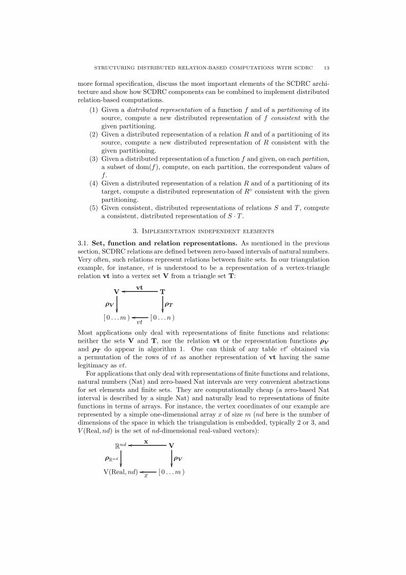
3.1. Set, function and relation representations. As mentioned in the previoussection, SCDRC relations are defined between zero-based intervals of natural numbers.Very often, such relations represent relations between finite sets. In our triangulationexample, for instance, vt is understood to be a representation of a vertex-trianglerelation vt into a vertex set V from a triangle set T:
V oo vtT
[ 0 . . .m )��
ρV
oo
vt[ 0 . . . n )
��
ρT
Most applications only deal with representations of finite functions and relations:neither the sets V and T, nor the relation vt or the representation functions ρV
and ρT do appear in algorithm 1. One can think of any table vt′ obtained viaa permutation of the rows of vt as another representation of vt having the samelegitimacy as vt.
For applications that only deal with representations of finite functions and relations,natural numbers (Nat) and zero-based Nat intervals are very convenient abstractionsfor set elements and finite sets. They are computationally cheap (a zero-based Natinterval is described by a single Nat) and naturally lead to representations of finitefunctions in terms of arrays. For instance, the vertex coordinates of our example arerepresented by a simple one-dimensional array x of size m (nd here is the number ofdimensions of the space in which the triangulation is embedded, typically 2 or 3, andV (Real, nd) is the set of nd-dimensional real-valued vectors):
Rnd oo x
V
V(Real, nd)��
ρRnd
oox [ 0 . . .m )
��
ρV
14 N. BOTTA, C. IONESCU, C. LINSTEAD, R. KLEIN
In turn, arrays of some generic type X, A(X), are, for many computational purposes,very efficient representations of finite functions.
An alternative approach for representing finite sets of a generic type X is by meansof a parameterized data structure: Set(X). Representations of finite sets-based onparameterized types are, of course, more powerful than representations-based onzero-based Nat interval abstractions. They can distinguish between sets of differenttypes but same cardinality. On the other hand, parameterized relation and functionrepresentations based on parameterized set representations – data structures of thekind Rel(Set(X), Set(Y)) or Fct(V(Real, nd), Set(Y)) in place of A(V(Real, nd)) forfunctions – make functions and relations dependent on application-specific, possiblyinefficient representations of set element types.
Notice that frameworks like Janus support parameterized representations of finitesets but rely on relations between zero-based Nat intervals. In SCDRC we onlyconsider sets, functions and relations which are finite. We adopt the Janus approachfor relations but we do not support parameterized representations of finite sets. Ofcourse, there are situations in SCDRC in which sets (most probably of Nats) have tobe explicitly represented. In these cases we use suitable containers like lists or arrays.
The analysis presented in this section is based on a simple conceptual representationof finite functions and relations as arrays of some type X and as arrays of arrays ofNats, respectively. We stress the fact that this is a conceptual model. As we will seein section 4, SCDRC relations are implemented by means of specific data structureslike CRS Rel and Reg Rel(n). While being isomorph to arrays of arrays of naturalnumbers (both CRS Rel and Reg Rel(n) can be constructed in terms of such anarray), SCDRC implementation of relations are defined in terms of an iterator-basedinterface which is very different from the array interface.
3.2. Distributed functions and distributed relations. In the list of problemspresented at the end of the previous section, we have used the term distributed rep-
resentation for functions and relations. In this paragraph we discuss such represen-tations. We follow the approach outlined above and think of functions and relationsas arrays of some type X and of type A(Nat), respectively. Let a be an array. Astraightforward way of distributing a on np partitions is:
(1) Cut a into np chunks.(2) Assign the first chunk to the first partition, the second chunk to the second
partition and so on.
For this partitioning scheme, the function pa :: [ 0 . . . np ) ←− [ 0 . . . size(a) ) thatassociates a partition number in [ 0 . . . np ) to each element of a is non-decreasing. Asusual, we represent pa with an array of Nats. Therefore, if size(a) == size(pa) >> np,pa can be more economically represented by an array of offsets (again of Nats) of sizenp + 1. In fact, any non-decreasing array ofs satisfying:
(2)
size(ofs) == np + 1
ofs(0) == 0
ofs(np) == size(a)
represents the non-decreasing partition function pa : [ 0 . . . np )←− [ 0 . . . ofs(np) ):
(3) ofs(p) <= k < ofs(p + 1) ≡ pa(k) == p
Conversely, given pa non-decreasing, the corresponding ofs can be easily computed:
STRUCTURING DISTRIBUTED RELATION-BASED COMPUTATIONS WITH SCDRC 15
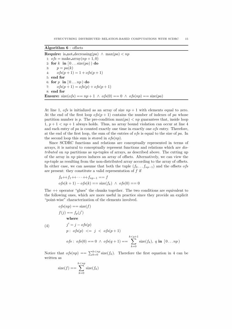
Algorithm 6 : offsets
Require: is not decreasing(pa) ∧ max(pa) < np1: ofs = make array(np + 1, 0)2: for k in [ 0 . . . size(pa) ) do
3: p = pa(k)4: ofs(p + 1) = 1 + ofs(p + 1)5: end for
6: for p in [ 0 . . . np ) do
7: ofs(p + 1) = ofs(p) + ofs(p + 1)8: end for
Ensure: size(ofs) == np + 1 ∧ ofs(0) == 0 ∧ ofs(np) == size(pa)
At line 1, ofs is initialized as an array of size np + 1 with elements equal to zero.At the end of the first loop ofs(p + 1) contains the number of indexes of pa whosepartition number is p. The pre-condition max(pa) < np guarantees that, inside loop1, p + 1 < np + 1 always holds. Thus, no array bound violation can occur at line 4and each entry of pa is counted exactly one time in exactly one ofs entry. Therefore,at the end of the first loop, the sum of the entries of ofs is equal to the size of pa. Inthe second loop this sum is stored in ofs(np).
Since SCDRC functions and relations are conceptually represented in terms ofarrays, it is natural to conceptually represent functions and relations which are dis-
tributed on np partitions as np-tuples of arrays, as described above. The cutting upof the array in np pieces induces an array of offsets. Alternatively, we can view thenp-tuple as resulting from the non-distributed array according to the array of offsets.In either case, we can assume that both the tuple (f0 . . . fnp−1) and the offsets ofsare present: they constitute a valid representation of f if
f0++f1++ · · ·++fnp−1 == f
ofs(k + 1)− ofs(k) == size(fk) ∧ ofs(0) == 0
The ++ operator “glues” the chunks together. The two conditions are equivalent tothe following ones, which are more useful in practice since they provide an explicit“point-wise” characterization of the elements involved.
(4)
ofs(np) == size(f)
f(j) == fp(j′)
where
j′ = j − ofs(p)
p : ofs(p) <= j < ofs(p + 1)
ofs : ofs(0) == 0 ∧ ofs(q + 1) ==
k<q+1∑
k=0
size(fk), q in [ 0 . . . np )
Notice that ofs(np) ==∑k<np
k=0 size(fk). Therefore the first equation in 4 can bewritten as
size(f) ==
k<np∑
k=0
size(fk)

16 N. BOTTA, C. IONESCU, C. LINSTEAD, R. KLEIN
which states an obvious size-consistency condition between f and (f0 . . . fnp−1). Sim-ilarly, (R0 . . . Rnp−1) is a distributed representations of R if:
ofs(np) == source size(R)
iRj == iRpj′
where
j′ = j − ofs(p)
p : ofs(p) <= j < ofs(p + 1)
ofs : ofs(0) == 0
∧
ofs(q + 1) ==
k<q+1∑
k=0
source size(Rk), q in [ 0 . . . np )
A caveat: just like the model for non-distributed functions and relations discussed inthe previous paragraph, the model discussed here for distributed functions and rela-tions is a conceptual one. It is essential for understanding the formal specification ofthe problems introduced in the next section. This model, however, does not mean thatthere are data structures, in SCDRC, representing a function or a relation togetherwith its corresponding offset or partitioning function. In much the same way, youwill not find, in SCDRC, functions that formally take tuple arguments that representdistributed functions or relations.
The scheme described above for distributing a one-dimensional array a on np par-titions and the corresponding conceptual representation of distributed functions andrelations is not new. This scheme is used in ParMetis where it is referred to as dis-tributed CRS format. In Janus, distributed relations are equipped with “descriptors”which contain, among others, informations about sizes and offsets of tuple represen-tations.
One can argue that there are many other ways of distributing an array a on nppartitions and some of them might be better than the scheme presented here. Forinstance, if some “communication” relation is defined between the chunks of a andbetween the partitions (these could be arranged, for a certain computational archi-tecture, according to some hardware “topology” that makes communication betweensome partitions faster that between others), one might want to “fit” the structure ofa to that of the computing architecture. Beside simplicity and minimality, anotherconsideration supports the conceptual model presented here: the problem of parti-tioning the source and the target of a relation for efficient distributed computations ofrelation-based algorithms is not trivial. As mentioned in the previous section, SCDRCdelegates the solution of this problem to external libraries like Metis and ParMetis.It is in the solution of the partitioning problem that additional, architecture specificpartitioning constraints can and should be naturally accounted for.
3.3. Problem specification. In this paragraph we give a formal specification of theproblems informally introduced at the end of section 2. This specification rests onthe conceptual representation of function and relations discussed in 3.1 and 3.2.
3.3.1. Problem 1. Given a distributed representation of a function f and of a parti-tioning of its source, compute a new distributed representation of f consistent with
STRUCTURING DISTRIBUTED RELATION-BASED COMPUTATIONS WITH SCDRC 17
the given partitioning.
Given:(f0 . . . fnp−1), fp :: A(X)(pf0 . . . pfnp−1), pfp :: A(Nat)
such that:i) size(fp) == size(pfp)ii) size(pfp) == 0 ∨ max elem(pfp) < np
find:(
f ′
0 . . . f ′
np−1
)
, f ′
p :: A(X)such that:
iii) f ′
p · permp == [ f(i) | i ∈ [ 0 . . . size(f) ) , pf(i) == p ]where
permp :: [ 0 . . .mp )←− [ 0 . . .mp ) is bijectivemp == size([ f(i) | i ∈ [ 0 . . . size(f) ) , pf(i) == p ]).
Let us comment on this specification: as discussed in 3.2, f is represented by a tupleof arrays, one array for each partition. On each partition, a partition function pfp
specifies how the elements of fp have to be redistributed among np partitions. Asusual, pfp is represented with an array. This has to have the same size as fp and hasto take values in [ 0 . . . np ). The solution of problem 1 is a new distributed functionf ′. Condition iii) requires f ′
p to contain exactly those values f(i) of f such thatpf(i) == p. Because of the permutation permp, these values can appear in any orderin f ′
p.In the above specification, we have assumed that non-empty arrays of Nats are
equipped with a function max elem :: Nat ←− A(Nat) that computes the maxi-mal element. max elem and size are examples of functions whose implementationdepends on the computational environment. The implementation of such functions inSCDRC’s SPSD and SPMD-distributed environments is discussed at the beginningof section 4. Let’s turn the attention to the second problem introduced at the end ofsection 2. The specification of problem 2 is completely analogous to that of problem1:
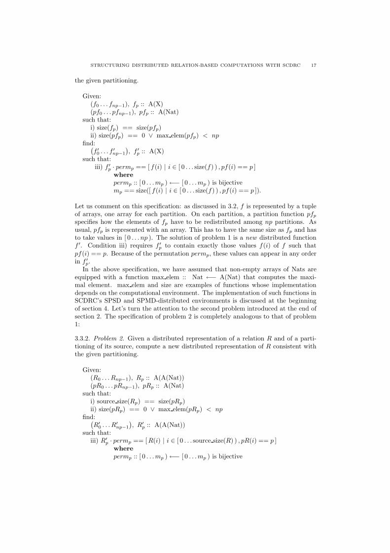
3.3.2. Problem 2. Given a distributed representation of a relation R and of a parti-tioning of its source, compute a new distributed representation of R consistent withthe given partitioning.
Given:(R0 . . . Rnp−1), Rp :: A(A(Nat))(pR0 . . . pRnp−1), pRp :: A(Nat)
such that:i) source size(Rp) == size(pRp)ii) size(pRp) == 0 ∨ max elem(pRp) < np
find:(
R′
0 . . . R′
np−1
)
, R′
p :: A(A(Nat))such that:
iii) R′
p · permp == [ R(i) | i ∈ [ 0 . . . source size(R) ) , pR(i) == p ]where
permp :: [ 0 . . .mp )←− [ 0 . . .mp ) is bijective
18 N. BOTTA, C. IONESCU, C. LINSTEAD, R. KLEIN
mp == size([ R(i) | i ∈ [ 0 . . . source size(R) ) , pR(i) == p ]).
Notice that, even in the case in which permp is taken to be the identity permutationon all partitions both in problem 1 and in problem 2, f ′, R′ are not, in general, equalto f and R. This is because of the fact that pf and pR have not been required to benon-decreasing. In other words, the repartitioning is not required to be a re-cutting.
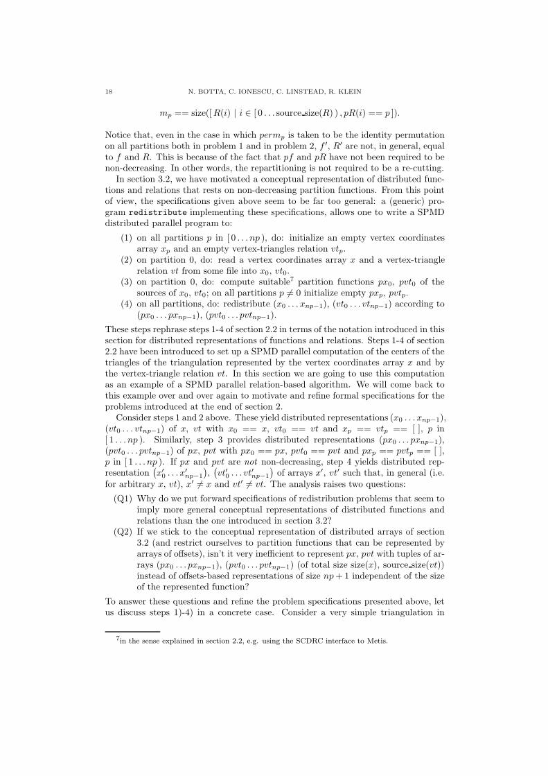
In section 3.2, we have motivated a conceptual representation of distributed func-tions and relations that rests on non-decreasing partition functions. From this pointof view, the specifications given above seem to be far too general: a (generic) pro-gram redistribute implementing these specifications, allows one to write a SPMDdistributed parallel program to:
(1) on all partitions p in [ 0 . . . np ), do: initialize an empty vertex coordinatesarray xp and an empty vertex-triangles relation vtp.
(2) on partition 0, do: read a vertex coordinates array x and a vertex-trianglerelation vt from some file into x0, vt0.
(3) on partition 0, do: compute suitable7 partition functions px0, pvt0 of thesources of x0, vt0; on all partitions p 6= 0 initialize empty pxp, pvtp.
(4) on all partitions, do: redistribute (x0 . . . xnp−1), (vt0 . . . vtnp−1) according to(px0 . . . pxnp−1), (pvt0 . . . pvtnp−1).
These steps rephrase steps 1-4 of section 2.2 in terms of the notation introduced in thissection for distributed representations of functions and relations. Steps 1-4 of section2.2 have been introduced to set up a SPMD parallel computation of the centers of thetriangles of the triangulation represented by the vertex coordinates array x and bythe vertex-triangle relation vt. In this section we are going to use this computationas an example of a SPMD parallel relation-based algorithm. We will come back tothis example over and over again to motivate and refine formal specifications for theproblems introduced at the end of section 2.
Consider steps 1 and 2 above. These yield distributed representations (x0 . . . xnp−1),(vt0 . . . vtnp−1) of x, vt with x0 == x, vt0 == vt and xp == vtp == [ ], p in[ 1 . . . np ). Similarly, step 3 provides distributed representations (px0 . . . pxnp−1),(pvt0 . . . pvtnp−1) of px, pvt with px0 == px, pvt0 == pvt and pxp == pvtp == [ ],p in [ 1 . . . np ). If px and pvt are not non-decreasing, step 4 yields distributed rep-resentation
(
x′
0 . . . x′
np−1
)
,(
vt′0 . . . vt′np−1
)
of arrays x′, vt′ such that, in general (i.e.for arbitrary x, vt), x′ 6= x and vt′ 6= vt. The analysis raises two questions:
(Q1) Why do we put forward specifications of redistribution problems that seem toimply more general conceptual representations of distributed functions andrelations than the one introduced in section 3.2?
(Q2) If we stick to the conceptual representation of distributed arrays of section3.2 (and restrict ourselves to partition functions that can be represented byarrays of offsets), isn’t it very inefficient to represent px, pvt with tuples of ar-rays (px0 . . . pxnp−1), (pvt0 . . . pvtnp−1) (of total size size(x), source size(vt))instead of offsets-based representations of size np + 1 independent of the sizeof the represented function?
To answer these questions and refine the problem specifications presented above, letus discuss steps 1)-4) in a concrete case. Consider a very simple triangulation in
7in the sense explained in section 2.2, e.g. using the SCDRC interface to Metis.
STRUCTURING DISTRIBUTED RELATION-BASED COMPUTATIONS WITH SCDRC 19
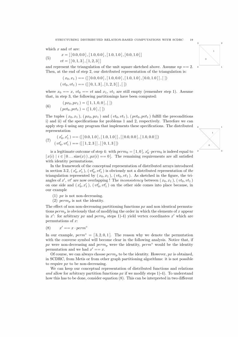
which x and vt are:
(5)x = [ [ 0.0, 0.0 ] , [ 1.0, 0.0 ] , [ 1.0, 1.0 ] , [ 0.0, 1.0 ] ]
vt = [ [ 0, 1, 3 ] , [ 1, 2, 3 ] ]
10
23
0
1
and represent the triangulation of the unit square sketched above. Assume np == 2.Then, at the end of step 2, our distributed representation of the triangulation is:
(x0, x1 ) == ([ [ 0.0, 0.0 ] , [ 1.0, 0.0 ] , [ 1.0, 1.0 ] , [ 0.0, 1.0 ] ] , [ ])
( vt0, vt1 ) == ([ [ 0, 1, 3 ] , [ 1, 2, 3 ] ] , [ ])
where x0 == x, vt0 == vt and x1, vt1 are still empty (remember step 1). Assumethat, in step 3, the following partitionings have been computed:
(6)( px0, px1 ) = ([ 1, 1, 0, 0 ] , [ ])
( pvt0, pvt1 ) = ([ 1, 0 ] , [ ])
The tuples (x0, x1 ), ( px0, px1 ) and ( vt0, vt1 ), ( pvt0, pvt1 ) fulfill the preconditionsi) and ii) of the specifications for problems 1 and 2, respectively. Therefore we canapply step 4 using any program that implements these specifications. The distributedrepresentation
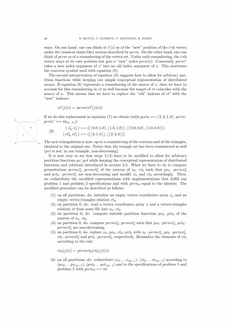
(7)(x′
0, x′
1 ) == ([ [ 0.0, 1.0 ] , [ 1.0, 1.0 ] ] , [ [ 0.0, 0.0 ] , [ 1.0, 0.0 ] ])
( vt′0, vt′1 ) == ([ [ 1, 2, 3 ] ] , [ [ 0, 1, 3 ] ])
0 1
2 3
0
1
is a legitimate outcome of step 4: with perm0 = [ 1, 0 ], x′
0 ·perm0 is indeed equal to[ x(i) | i ∈ [ 0 . . . size(x) ) , px(i) == 0 ]. The remaining requirements are all satisfiedwith identity permutations.
In the framework of the conceptual representation of distributed arrays introducedin section 3.2, ( x′
0, x′
1 ), ( vt′0, vt′1 ) is obviously not a distributed representation of the
triangulation represented by (x0, x1 ), ( vt0, vt1 ). As sketched in the figure, the tri-angles of x′, vt′ are now overlapping ! The inconsistency between (x0, x1 ), ( vt0, vt1 )on one side and (x′
0, x′
1 ), ( vt′0, vt′1 ) on the other side comes into place because, inour example
(1) px is not non-decreasing.(2) permp is not the identity.
The effect of non non-decreasing partitioning functions px and non identical permuta-tions permp is obviously that of modifying the order in which the elements of x appearin x′: for arbitrary px and permp steps 1)-4) yield vertex coordinates x′ which arepermutations of x:
(8) x′ == x · perm◦
In our example, perm◦ = [ 3, 2, 0, 1 ]. The reason why we denote the permutationwith the converse symbol will become clear in the following analysis. Notice that, ifpx were non-decreasing and permp were the identity, perm◦ would be the identitypermutation and we had x′ == x.
Of course, we can always choose permp to be the identity. However, px is obtained,in SCDRC, from Metis or from other graph partitioning algorithms: it is not possibleto require px to be non-decreasing.
We can keep our conceptual representation of distributed functions and relationsand allow for arbitrary partition functions px if we modify steps 1)-4). To understandhow this has to be done, consider equation (8). This can be interpreted in two different
20 N. BOTTA, C. IONESCU, C. LINSTEAD, R. KLEIN
ways. On one hand, one can think of x′(i) as of the “new” position of the i-th vertexunder the (musical chairs like) motion described by perm. On the other hand, one canthink of perm as of a renumbering of the vertex set. Under such renumbering, the i-thvertex stays at its own position but gets a “new” index perm(i). Conversely, perm◦
takes a new index argument of x′ into an old index argument of x. This motivatesthe converse symbol used with equation (8).
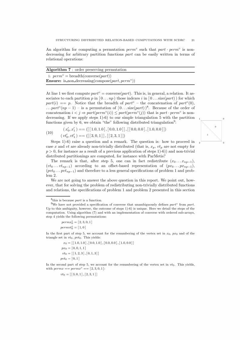
The second interpretation of equation (8) suggests how to allow for arbitrary par-tition functions while keeping our simple conceptual representation of distributedarrays. If equation (8) represents a renumbering of the source of x, then we have toaccount for this renumbering in vt as well because the target of vt coincides with thesource of x. This means that we have to replace the “old” indexes of vt′ with the“new” indexes:
vt′(j)(i)← perm(vt′(j)(i))
If we do this replacement in equation (7) we obtain (with perm == [ 2, 3, 1, 0 ] , perm ·perm◦ == id[ 0...4 )):
0 1
2 3
1
0
(9)( x′
0, x′
1 ) == ([ [ 0.0, 1.0 ] , [ 1.0, 1.0 ] ] , [ [ 0.0, 0.0 ] , [ 1.0, 0.0 ] ])
( vt′0, vt′1 ) == ([ [ 3, 1, 0 ] ] , [ [ 2, 3, 0 ] ])
The new triangulation is now, up to a renumbering of the vertexes and of the triangles,identical to the original one. Notice that the triangle set has been renumbered as well(pvt is not, in our example, non-decreasing).
It is now easy to see how steps 1)-4) have to be modified to allow for arbitrarypartition functions px, pvt while keeping the conceptual representation of distributedfunctions and relations introduced in section 3.2. What we have to do is computepermutations permx◦
0, permvt◦0 of the sources of x0, vt0 such that px0 · permx◦
0
and pvt0 · permvt◦0 are non-decreasing and modify x0 and vt0 accordingly. Then,we redistribute the modified representations with implementations that fulfill ourproblem 1 and problem 2 specifications and with permd equal to the identity. Themodified procedure can be described as follows:
(1) on all partitions, do: initialize an empty vertex coordinates array xp and anempty vertex-triangles relation vtp.
(2) on partition 0, do: read a vertex coordinates array x and a vertex-trianglesrelation vt from some file into x0, vt0.
(3) on partition 0, do: compute suitable partition functions px0, pvt0 of thesources of x0, vt0.
(4) on partition 0, do: compute permx◦
0, permvt◦0 such that px0 · permx◦
0, pvt0 ·permvt◦0 are non-decreasing.
(5) on partition 0, do: replace x0, px0, vt0, pvt0 with x0 · permx◦
0, px0 · permx◦
0,vt0 · permvt◦0 and pvt0 · permvt◦0, respectively. Renumber the elements of vt0according to the rule
vt0(j)(i)← permvt0(vt0(j)(i))
(6) on all partitions, do: redistribute (x0 . . . xnp−1), (vt0 . . . vtnp−1) according to(px0 . . . pxnp−1), (pvt0 . . . pvtnp−1) and to the specifications of problem 1 andproblem 2 with permd == id.
STRUCTURING DISTRIBUTED RELATION-BASED COMPUTATIONS WITH SCDRC 21
An algorithm for computing a permutation perm◦ such that part · perm◦ is non-decreasing for arbitrary partition functions part can be easily written in terms ofrelational operations:
Algorithm 7 : order preserving permutation
1: perm◦ = breadth(converse(part))Ensure: is non decreasing(compose(part, perm◦))
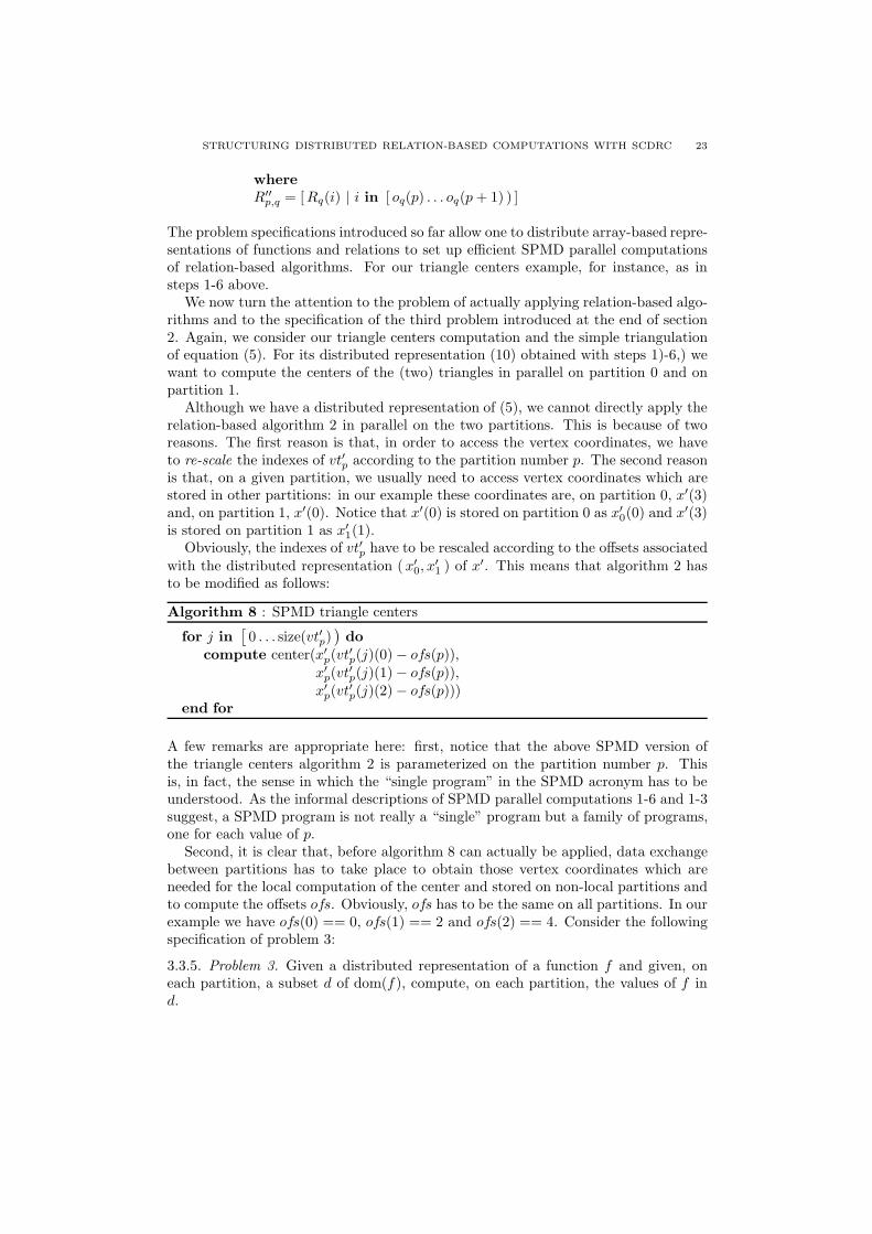
At line 1 we first compute part◦ = converse(part). This is, in general, a relation. It as-sociates to each partition p in [ 0 . . . np ) those indexes i in [ 0 . . . size(part) ) for whichpart(i) == p. Notice that the breadth of part◦ – the concatenation of part◦(0),. . . part◦(np − 1) – is a permutation of [ 0 . . . size(part) )8. Because of the order ofconcatenation i < j ⇒ part(perm◦(i)) ≤ part(perm◦(j)) that is part · perm◦ is non-decreasing. If we apply steps 1)-6) to our simple triangulation 5 with the partitionfunctions given by 6, we obtain “the” following distributed triangulation9:
(10)(x′
0, x′
1 ) == ([ [ 1.0, 1.0 ] , [ 0.0, 1.0 ] ] , [ [ 0.0, 0.0 ] , [ 1.0, 0.0 ] ])
( vt′0, vt′1 ) == ([ [ 3, 0, 1 ] ] , [ [ 2, 3, 1 ] ])
2 3
1
0
01
Steps 1)-6) raise a question and a remark. The question is: how to proceed incase x and vt are already non-trivially distributed (that is, xp, vtp are not empty forp > 0, for instance as a result of a previous application of steps 1)-6)) and non-trivialdistributed partitionings are computed, for instance with ParMetis?
The remark is that, after step 5, one can in fact redistribute (x0 . . . xnp−1),(vt0 . . . vtnp−1) according to an offset-based representation of (px0 . . . pxnp−1),(pvt0 . . . pvtnp−1) and therefore to a less general specifications of problem 1 and prob-lem 2.
We are not going to answer the above question in this report. We point out, how-ever, that for solving the problem of redistributing non-trivially distributed functionsand relations, the specifications of problem 1 and problem 2 presented in this section
8this is because part is a function.9We have not provided a specification of converse that unambiguously defines part◦ from part.
Up to this ambiguity, however, the outcome of steps 1)-6) is unique. Here we detail the steps of thecomputation. Using algorithm (7) and with an implementation of converse with ordered sub-arrays,step 4 yields the following permutations:
permx◦0 = [ 2, 3, 0, 1 ]
permvt◦0 = [ 1, 0 ]
In the first part of step 5, we account for the renumbering of the vertex set in x0, px0 and of thetriangle set in vt0, pvt0. This yields:
x0 = [ [ 1.0, 1.0 ] , [ 0.0, 1.0 ] , [ 0.0, 0.0 ] , [ 1.0, 0.0 ] ]
px0 = [ 0, 0, 1, 1 ]
vt0 = [ [ 1, 2, 3 ] , [ 0, 1, 3 ] ]
pvt0 = [ 0, 1 ]
In the second part of step 5, we account for the renumbering of the vertex set in vt0. This yields,with permx == permx◦ == [ 2, 3, 0, 1 ]:
vt0 = [ [ 3, 0, 1 ] , [ 2, 3, 1 ] ]

22 N. BOTTA, C. IONESCU, C. LINSTEAD, R. KLEIN
play an important role. This partially answers question Q1. For the purpose of im-plementing steps 1)-6), it is indeed meaningful to introduce less general specifications.This is what we are going to do next, thereby answering question Q2.
One can think of steps 1)-5) as of pre-processing steps that generate some triangu-lation file. This file contains a vertex coordinates array x, a vertex-triangles relationvt and two offsets arrays ox and ovt. Steps 1)-6) can be then rephrased as follows:
(1) on all partitions p in [ 0 . . . np ), initialize an empty vertex coordinates arrayxp, an empty vertex-triangles relation vtp and empty offsets arrays oxp andovtp.
(2) on partition 0, read a vertex coordinates array x, a vertex-triangles relationvt and offsets arrays ox and ovt from some file into x0, vt0, ox0 and ovt0.
(3) on all partitions, redistribute (x0 . . . xnp−1), (vt0 . . . vtnp−1) according to(ox0 . . . oxnp−1), (ovt0 . . . ovtnp−1).
Implementations of Step 3) are now required to fulfill the following specifications:
3.3.3. Problem 1’. Given a distributed representation of a function f and given apartitioning of its source, compute a new distributed representation of f consistentwith the given partitioning.
Given:(f0 . . . fnp−1), fp :: A(X)(o0 . . . onp−1), op :: A(Nat)
such that:i) is offsets(op)ii) size(op) == np + 1iii) size(fp) == op(np)
find:(
f ′
0 . . . f ′
np−1
)
, f ′
p :: A(X)such that:
iv) f ′
p == concat(
f ′′
p,0 . . . f ′′
p,np−1
)
where
f ′′
p,q = [ fq(i) | i in [ oq(p) . . . oq(p + 1) ) ]
3.3.4. Problem 2’. Given a distributed representation of a relation R and given a par-titioning of its source, compute a new distributed representation of R consistent withthe given partitioning.
Given:(R0 . . . Rnp−1), Rp :: A(A(Nat))(o0 . . . onp−1), op :: A(Nat)
such that:i) is offsets(op)ii) size(op) == np + 1iii) source size(Rp) == op(np)
find:(
R′
0 . . . R′
np−1
)
, R′
p :: A(A(Nat))such that:
iv) R′
p == concat(
R′′
p,0 . . . R′′
p,np−1
)
STRUCTURING DISTRIBUTED RELATION-BASED COMPUTATIONS WITH SCDRC 23
where
R′′
p,q = [ Rq(i) | i in [ oq(p) . . . oq(p + 1) ) ]
The problem specifications introduced so far allow one to distribute array-based repre-sentations of functions and relations to set up efficient SPMD parallel computationsof relation-based algorithms. For our triangle centers example, for instance, as insteps 1-6 above.
We now turn the attention to the problem of actually applying relation-based algo-rithms and to the specification of the third problem introduced at the end of section2. Again, we consider our triangle centers computation and the simple triangulationof equation (5). For its distributed representation (10) obtained with steps 1)-6,) wewant to compute the centers of the (two) triangles in parallel on partition 0 and onpartition 1.
Although we have a distributed representation of (5), we cannot directly apply therelation-based algorithm 2 in parallel on the two partitions. This is because of tworeasons. The first reason is that, in order to access the vertex coordinates, we haveto re-scale the indexes of vt′p according to the partition number p. The second reasonis that, on a given partition, we usually need to access vertex coordinates which arestored in other partitions: in our example these coordinates are, on partition 0, x′(3)and, on partition 1, x′(0). Notice that x′(0) is stored on partition 0 as x′
0(0) and x′(3)is stored on partition 1 as x′
1(1).Obviously, the indexes of vt′p have to be rescaled according to the offsets associated
with the distributed representation (x′
0, x′
1 ) of x′. This means that algorithm 2 hasto be modified as follows:
Algorithm 8 : SPMD triangle centers
for j in[
0 . . . size(vt′p))
do
compute center(x′
p(vt′p(j)(0)− ofs(p)),x′
p(vt′p(j)(1)− ofs(p)),x′
p(vt′p(j)(2)− ofs(p)))end for
A few remarks are appropriate here: first, notice that the above SPMD version ofthe triangle centers algorithm 2 is parameterized on the partition number p. Thisis, in fact, the sense in which the “single program” in the SPMD acronym has to beunderstood. As the informal descriptions of SPMD parallel computations 1-6 and 1-3suggest, a SPMD program is not really a “single” program but a family of programs,one for each value of p.
Second, it is clear that, before algorithm 8 can actually be applied, data exchangebetween partitions has to take place to obtain those vertex coordinates which areneeded for the local computation of the center and stored on non-local partitions andto compute the offsets ofs. Obviously, ofs has to be the same on all partitions. In ourexample we have ofs(0) == 0, ofs(1) == 2 and ofs(2) == 4. Consider the followingspecification of problem 3:
3.3.5. Problem 3. Given a distributed representation of a function f and given, oneach partition, a subset d of dom(f), compute, on each partition, the values of f ind.
24 N. BOTTA, C. IONESCU, C. LINSTEAD, R. KLEIN
Given:(f0 . . . fnp−1), fp :: A(X)(d0 . . . dnp−1), dp :: A(Nat)
such that:i) max elem(dp) < ofs(np)
where
ofs = offsets(map(size, (f0 . . . fnp−1)))find:
(fd0 . . . fdnp−1), fdp :: A(X)such that:
ii) size(fdp) == size(dp)iii) fdp(i) == f(dp(i))
Here, the generic function offsets and the function map fulfill:
offsets :: A(Nat)←− Natn
ofs == offsets(s0 . . . sn−1)≡size(ofs) == n + 1 ∧ ofs(0) == 0 ∧ ofs(p + 1) ==
∑k<p+1k=0 sk
map :: A(X) ←− (X←− Y)×Yn
ax == map (f, (y0 . . . yn−1))≡ax(k) == f(yk), k = [ 0 . . . n )
With a dom complete program implementing the above specification of problem 3and with an implementation of algorithm 8, it is easy to write a SPMD program tocompute the triangle centers. All we have to do is to:
(1) Apply dom complete and complete the data(
x′
0 . . . x′
np−1
)
on(
breadth(vt′0) . . .breadth(vt′np−1))
. This yields the arrays(
x′′
0 . . . x′′
np−1
)
.(2) Apply algorithm 8 with x′′
p(3 ∗ j + i) in place of x′
p(vt′p(j)(i) − ofs(p)).
In our example, step 1 yields x′′
0 = [ [ 1.0, 0.0 ] , [ 1.0, 1.0 ] , [ 0.0, 1.0 ] ] andx′′
1 = [ [ 0.0, 0.0 ] , [ 1.0, 0.0 ] , [ 0.0, 1.0 ] ]. Step 2) provides the centers [ 2/3, 2/3 ], [ 1/3, 1/3 ]on partitions 0 and 1, respectively. These are indeed the coordinates of the centers ofthe triangles 0 and 1 of the figure on the left of equation (10).
There are two major problems with the approach outlined above. The first problemis that we are duplicating too much data. Remember that, if we accept to duplicate a
lot of data, the problem of structuring SPMD parallel computations becomes trivial10:we simply store the whole x′ on all partitions. Here we increase the memory allocationcosts for x′ by a factor size(vt′)) instead of np∗size(x′). On large, plane triangulations,however, the number of triangles is about twice the number of nodes and we storethree x′-values per triangle. Thus, the ratio between np ∗ size(x′) and size(vt′)) isabout np/6. This means that we need at least 6 partitions for our scheme to becompetitive with the simple minded, full duplication approach: this is not good.
Notice that, in many applications, the ratio between the memory required to storean x′ element and the memory required to store a Nat can be quite large. In our
10if we let apart the problem of ensuring the consistency of the duplicated data.
STRUCTURING DISTRIBUTED RELATION-BASED COMPUTATIONS WITH SCDRC 25
example, x′ elements are arrays of 2 doubles. The ratio between sizeof(double) andsizeof(Nat) is, e.g., on my computing architecture, equal to four. This ratio wouldbe six if the triangulation were embedded in a three-dimensional space.
Also notice that, if we have been able to partition the original triangulations “well”,the number of x′-values which are needed for the local triangle centers computationbut which are stored on remote partitions will be much smaller than the number ofx′-values which are stored locally.
The above remarks suggest a more efficient scheme for storing and accessing thex′-values retrieved from remote partitions. What we want to do is:
(1) Extend x′
p with those values of x′ which are needed for the local trianglecenters computation but which are stored on remote partitions.
(2) Construct an auxiliary access table vt′′p such that
x′
p(vt′′p(j)(k)) == x′(vt′(j)(k))
This approach has been originally proposed in the Janus framework and has beenadopted in SCDRC. The second problem that affects triangle centers computationsbased on the specification of problem 3 given above is more subtle. Although we havenot discussed how a dom complete program could be implemented, it is obvious that,in order to compute a tuple (fd0 . . . fdnp−1), the following steps have to be done:
a) on each partition p, do: compute the indexes of dp (in our example dp =breadth(vt′p)) which are in [ ofs(q) . . . ofs(q + 1) ) for partitions q 6= p.
b) On each partition p, do: compute the indexes of [ ofs(p) . . . ofs(p) + size(fp) )which are in dq for partitions q 6= p.
While the first table can be computed without additional data exchange betweenpartitions11, the computation of the second table certainly requires communicationbetween partitions. It is only after each partition p knows, for any partition q 6=p, which are the indexes whose correspondent f -values have to be sent that suchvalues can actually be exchanged. The cost of computing such exchange tables cansignificantly exceed the cost of exchanging the f -values themselves. The same is truefor the cost of computing access tables like the auxiliary relation vt′′p discussed above.
These exchange and access tables do not depend on the data to be actually ex-changed but only on the set of indexes on which f has to be evaluated on a givenpartition and, of course, on the partitioning of f itself.
In many practical cases, the parallel computation of relation-based algorithms isrequired at each step of some iterative procedure in which the values of f changefrom step to step but the exchange and access tables do not. In our triangle centersexample, for instance, the vertex coordinates could change from step to step (e.g.because of forces acting on the triangulation) while the vertex triangle relation andthe partitioning of the vertex coordinates stay the same. In the iterative solution ofimplicit problems (e.g. linear systems of equations) relation-based algorithms thatrepresent the action of some discrete operator on a “vector of unknowns” might beevaluated thousands of times. At each time the values of the “unknowns” wouldchange but the relation and the partitioning scheme for such values would not.
Thus, for many practical cases, it would be very inefficient to recompute, at eachiteration step, the tables needed to exchange data between partitions and to efficiently
11w.r.t. the data exchange required to compute ofs.
26 N. BOTTA, C. IONESCU, C. LINSTEAD, R. KLEIN
access the local data. Therefore it is particularly important to decouple the computa-tion of the exchange and access tables from the actual data exchange. This motivatesthe specification of the following problem:
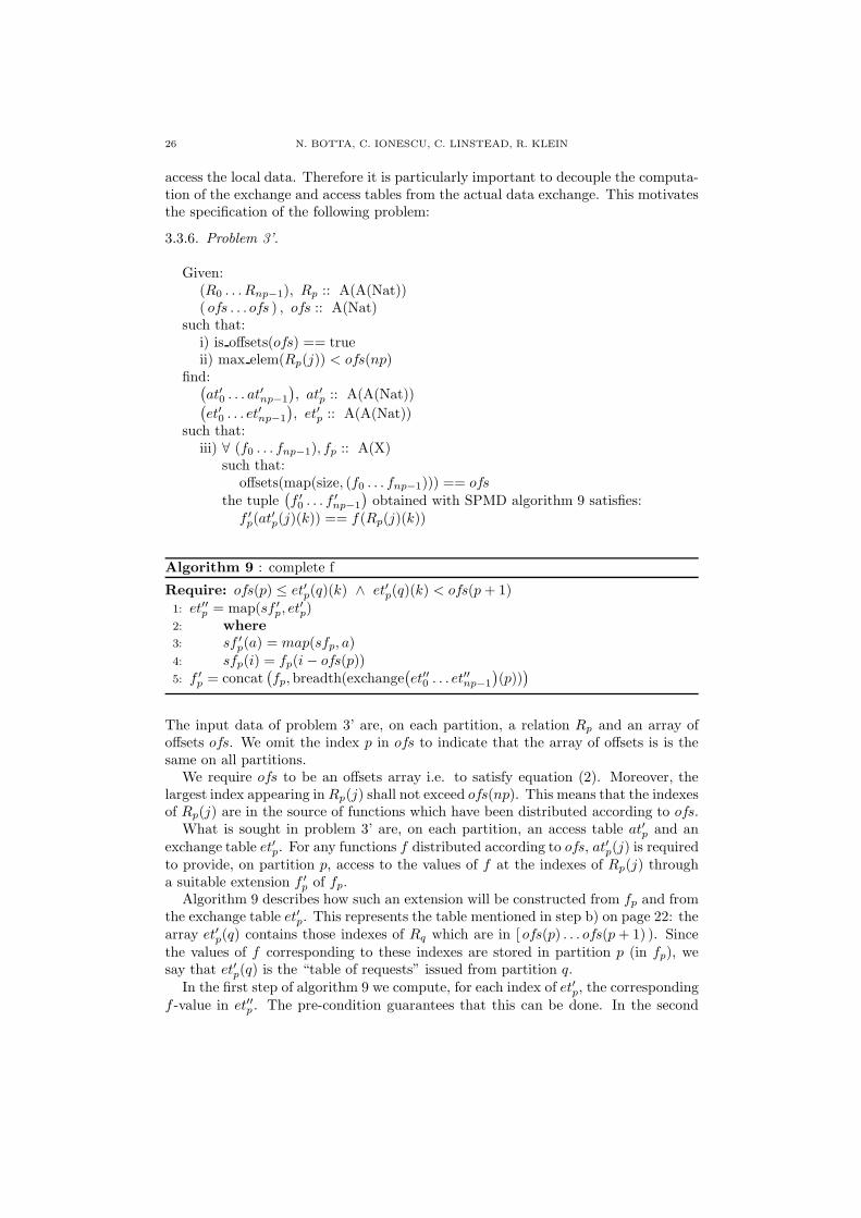
3.3.6. Problem 3’.
Given:(R0 . . . Rnp−1), Rp :: A(A(Nat))( ofs . . . ofs ) , ofs :: A(Nat)
such that:i) is offsets(ofs) == trueii) max elem(Rp(j)) < ofs(np)
find:(
at′0 . . . at′np−1
)
, at′p :: A(A(Nat))(
et′0 . . . et′np−1
)
, et′p :: A(A(Nat))such that:
iii) ∀ (f0 . . . fnp−1), fp :: A(X)such that:
offsets(map(size, (f0 . . . fnp−1))) == ofsthe tuple
(
f ′
0 . . . f ′
np−1
)
obtained with SPMD algorithm 9 satisfies:f ′
p(at′p(j)(k)) == f(Rp(j)(k))
Algorithm 9 : complete f
Require: ofs(p) ≤ et′p(q)(k) ∧ et′p(q)(k) < ofs(p + 1)1: et′′p = map(sf ′
p, et′
p)2: where
3: sf ′
p(a) = map(sfp, a)4: sfp(i) = fp(i− ofs(p))5: f ′
p = concat(
fp, breadth(exchange(
et′′0 . . . et′′np−1
)
(p)))
The input data of problem 3’ are, on each partition, a relation Rp and an array ofoffsets ofs. We omit the index p in ofs to indicate that the array of offsets is is thesame on all partitions.
We require ofs to be an offsets array i.e. to satisfy equation (2). Moreover, thelargest index appearing in Rp(j) shall not exceed ofs(np). This means that the indexesof Rp(j) are in the source of functions which have been distributed according to ofs.
What is sought in problem 3’ are, on each partition, an access table at′p and anexchange table et′p. For any functions f distributed according to ofs, at′p(j) is requiredto provide, on partition p, access to the values of f at the indexes of Rp(j) througha suitable extension f ′
p of fp.Algorithm 9 describes how such an extension will be constructed from fp and from
the exchange table et′p. This represents the table mentioned in step b) on page 22: thearray et′p(q) contains those indexes of Rq which are in [ ofs(p) . . . ofs(p + 1) ). Sincethe values of f corresponding to these indexes are stored in partition p (in fp), wesay that et′p(q) is the “table of requests” issued from partition q.
In the first step of algorithm 9 we compute, for each index of et′p, the correspondingf -value in et′′p . The pre-condition guarantees that this can be done. In the second
STRUCTURING DISTRIBUTED RELATION-BASED COMPUTATIONS WITH SCDRC 27
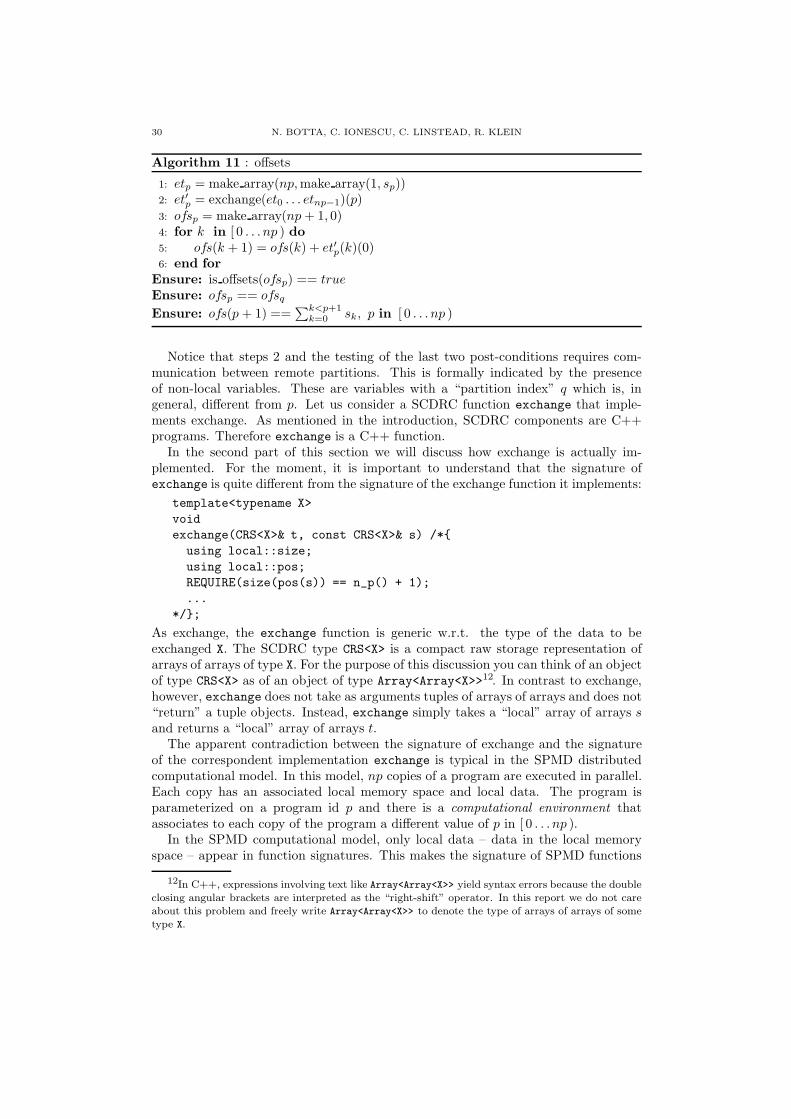
step we exchange the table of f values et′′p between partitions. The function exchangeplays an outstanding role in SCDRC. Although SCDRC users will almost never callexchange directly, most SCDRC algorithms that require data communication betweenpartitions are designed around this communication primitive. We will come back tothe implementation of exchange in section 4. Here we provide its specification:
exchange :: A(A(X))np ←− A(A(X))np(
et′0 . . . et′np−1
)
== exchange(et0 . . . etnp−1)≡is in(x, et′p(q)) == is in(x, etq(p))
We read the specification in the following way: x is an element that partition p receivesfrom partition q iff x is an element that partition q sends to partition p.
After having exchanged et′′p between partitions, we obtain, in line 4 of algorithm9 a tuple of arrays of arrays of elements of the same type of the elements of f . Onpartition p, the p-th array of the tuple is flattened and concatenated with fp.
If we have an exchange program that implements the specification of exchange, itis easy to write a complete program that implements algorithm 9. Also implementinga program access exch table that fulfills 3’ is not difficult if exchange is available:tables of requests etp can be computed locally by sorting the elements of Rp whosef -values are stored on remote partitions according to their correspondent partitionnumber. A call to exchange yields then the exchange tables et′p. The computationof the access tables at′p is a little bit less straightforward.
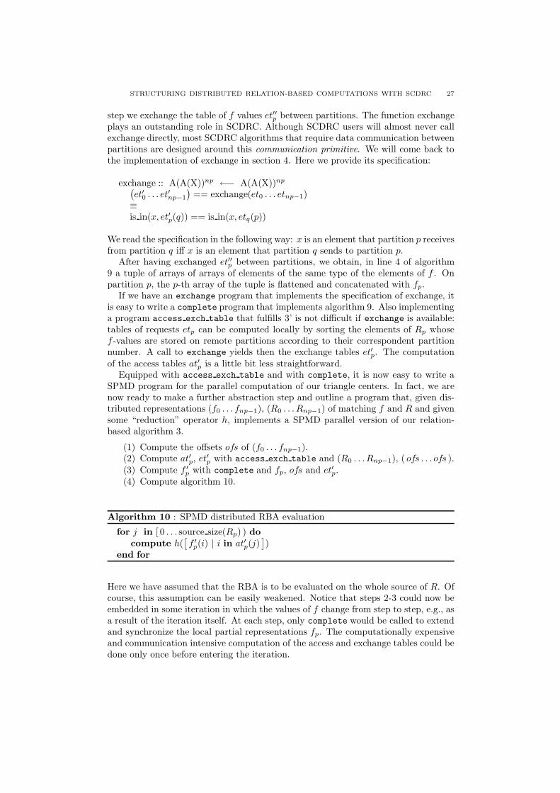
Equipped with access exch table and with complete, it is now easy to write aSPMD program for the parallel computation of our triangle centers. In fact, we arenow ready to make a further abstraction step and outline a program that, given dis-tributed representations (f0 . . . fnp−1), (R0 . . . Rnp−1) of matching f and R and givensome “reduction” operator h, implements a SPMD parallel version of our relation-based algorithm 3.
(1) Compute the offsets ofs of (f0 . . . fnp−1).(2) Compute at′p, et′p with access exch table and (R0 . . . Rnp−1), ( ofs . . . ofs ).(3) Compute f ′
p with complete and fp, ofs and et′p.(4) Compute algorithm 10.
Algorithm 10 : SPMD distributed RBA evaluation
for j in [ 0 . . . source size(Rp) ) do
compute h([
f ′
p(i) | i in at′p(j)]
)end for
Here we have assumed that the RBA is to be evaluated on the whole source of R. Ofcourse, this assumption can be easily weakened. Notice that steps 2-3 could now beembedded in some iteration in which the values of f change from step to step, e.g., asa result of the iteration itself. At each step, only complete would be called to extendand synchronize the local partial representations fp. The computationally expensiveand communication intensive computation of the access and exchange tables could bedone only once before entering the iteration.
28 N. BOTTA, C. IONESCU, C. LINSTEAD, R. KLEIN
The algorithm outlined above shows how parallel SPMD computations of rela-tion based algorithms can be structured using software components provided by SC-DRC. As mentioned in the introduction, these components – e.g. access exch table,complete and components representing RBAs themselves – are designed to supportstructured user control over communication steps. They allow to distinguish betweenthe kind of communication that takes place in steps 1 and 2 from the communica-tion needed to exchange f -values. However, developers of SCDRC do not need tocare about message passing level communication and related synchronization, mutualexclusion, deadlock or race condition problems.
Of course, developers of SCDRC-based, application dependent software are free tohide some of these communication steps and aggregate functionalities in more spe-cific components. For instance, a software component representing a vertex-centeredLaplace operator on triangulations could be defined in terms of RBAs in which R andh are fixed. Users could be enabled to construct concrete instances of such Laplaceoperator by simply passing a distributed function f of the vertexes of the triangulationto suitable constructors. These, in turn, could automatically call RBA constructorsand access exch table functionalities to set up a parallel evaluation of the Laplaceoperator without further user intervention.
In section 2, we have mentioned the problem of combining grid relations for com-puting neighborhood relationships and motivated the implementation of simple basicrelational operations. We close this section with the specifications of the problems ofparallel conversing a distributed relation and of composing two distributed relations.
3.3.7. Problem 4. Given a distributed representation of a relation R and of a parti-tioning of its target, compute a distributed representation of R◦ consistent with thegiven partitioning.
Given:(R0 . . . Rnp−1), Rp :: A(A(Nat))( ofs . . . ofs ) , ofs :: A(Nat)
such that:i) is offsets(ofs) == trueii) max elem(Rp(j)) < ofs(np)
find:(
R◦
0 . . . R◦
np−1
)
, R◦
p :: A(A(Nat))such that:
iii) offsets(
size(R◦
0) . . . size(R◦
np−1))
iv) iRj ≡ jR◦i
3.3.8. Problem 5. Given consistent, distributed representations of relations S and T ,compute a consistent, distributed representation of S · T .
Given:(S0 . . . Snp−1), Sp :: A(A(Nat))(T0 . . . Tnp−1), Tp :: A(A(Nat))
such that:i) max elem(Tp(j)) < offsets(map(source size, (S0 . . . Snp−1)))(np)
find:
STRUCTURING DISTRIBUTED RELATION-BASED COMPUTATIONS WITH SCDRC 29
(R0 . . . Rnp−1), Rp :: A(A(Nat))such that:
ii) source size(Rp) == source size(Tp)iii) iSk ∧ kRj ≡ iRj
4. Implementation dependent elements
In this section we present and discuss implementation dependent aspects of SC-DRC. In the first part we outline the architecture of SCDRC. In particular, we explainthe approach used to represent the two computational environments of SCDRC, wedescribe the file system structure and the most important SCDRC components andwe explain how SCDRC is documented.
In the second part we discuss a small number of data structures and functions insome detail. These functionalities are going to be used in the next and last sectionto set up a simple SPMD parallel application. As you might have guessed this isthe relation-based algorithm example we have been using throughout this report: thecomputation of the centers of the triangles of a distributed triangulation.
4.1. Computational environments and namespaces. In the previous section wehave discussed formal specifications for the problems introduced at the end of section2. The specifications are based on the conceptual model of distributed functions andrelations discussed in section 3.2: in this model, distributed functions and relations arerepresented by tuples of arrays. Accordingly, functions acting on distributed functionsand relations take arguments which are tuples of arrays. In general, functions actingof distributed data take tuple arguments.
This is clearly visible in the signature of exchange and has been implicitly assumedfor functions like offsets, complete etc. Let us have a closer look at offsets. A specifi-cation for this function can be expressed as follows:
offsets :: A(Nat)np ←− Natnp
(ofs0 . . . ofsnp−1) == offsets(s0 . . . snp−1)≡is offsets(ofsp) == true∧ofsp == ofsq
∧ofs(p + 1) ==
∑k<p+1k=0 sk, p in [ 0 . . . np )
With a function exchange fulfilling the specification given in section 4, it is easy towrite a SPMD algorithm that implements the above specification:As usual, the algorithm is parameterized on the partition number p. At line 1 weconstruct an array etp of np elements. Each element of etp is itself an array of Natsof size one and contains the single value sp. Therefore etp(q)(0) == sp independentlyof q. That is, each partition sends its local size sp to all other partitions. Afterexchange, et′p contains np arrays of Nats of size one. According to the specification ofexchange, et′p(q)(0) == sq independently of p. This means that et′p is the same tableon all partitions. Thus, in the loop at lines 4-6, the same offset array is computed onall partitions.
30 N. BOTTA, C. IONESCU, C. LINSTEAD, R. KLEIN
Algorithm 11 : offsets
1: etp = make array(np, make array(1, sp))2: et′p = exchange(et0 . . . etnp−1)(p)3: ofsp = make array(np + 1, 0)4: for k in [ 0 . . . np ) do
5: ofs(k + 1) = ofs(k) + et′p(k)(0)6: end for
Ensure: is offsets(ofsp) == trueEnsure: ofsp == ofsq
Ensure: ofs(p + 1) ==∑k<p+1
k=0 sk, p in [ 0 . . . np )
Notice that steps 2 and the testing of the last two post-conditions requires com-munication between remote partitions. This is formally indicated by the presenceof non-local variables. These are variables with a “partition index” q which is, ingeneral, different from p. Let us consider a SCDRC function exchange that imple-ments exchange. As mentioned in the introduction, SCDRC components are C++programs. Therefore exchange is a C++ function.
In the second part of this section we will discuss how exchange is actually im-plemented. For the moment, it is important to understand that the signature ofexchange is quite different from the signature of the exchange function it implements:
template<typename X>
void
exchange(CRS<X>& t, const CRS<X>& s) /*{
using local::size;
using local::pos;
REQUIRE(size(pos(s)) == n_p() + 1);
...
*/};
As exchange, the exchange function is generic w.r.t. the type of the data to beexchanged X. The SCDRC type CRS<X> is a compact raw storage representation ofarrays of arrays of type X. For the purpose of this discussion you can think of an objectof type CRS<X> as of an object of type Array<Array<X>>12. In contrast to exchange,however, exchange does not take as arguments tuples of arrays of arrays and does not“return” a tuple objects. Instead, exchange simply takes a “local” array of arrays sand returns a “local” array of arrays t.
The apparent contradiction between the signature of exchange and the signatureof the correspondent implementation exchange is typical in the SPMD distributedcomputational model. In this model, np copies of a program are executed in parallel.Each copy has an associated local memory space and local data. The program isparameterized on a program id p and there is a computational environment thatassociates to each copy of the program a different value of p in [ 0 . . . np ).
In the SPMD computational model, only local data – data in the local memoryspace – appear in function signatures. This makes the signature of SPMD functions
12In C++, expressions involving text like Array<Array<X>> yield syntax errors because the doubleclosing angular brackets are interpreted as the “right-shift” operator. In this report we do not careabout this problem and freely write Array<Array<X>> to denote the type of arrays of arrays of sometype X.

STRUCTURING DISTRIBUTED RELATION-BASED COMPUTATIONS WITH SCDRC 31
similar to their SPSD (single program single data) sequential counterpart. In theSPMD computational model, the visibility of local data is controlled by the samescoping rules as in the SPSD model. SPMD functions, however, can also access non-local data via communication between remote partitions. This can be done becausethe computational environment provides, beside the local program id p, the totalnumber of program copies np and suitable communication primitives.
The absence of explicit representation of non-local argument data in the signa-ture of SPMD functions is often a source of ambiguity and confusion. It makes itchallenging to design software which is easily understandable.
Consider a simple size function that computes the size of an array. In a SPSDcomputational environment size has the following signature:
(11) size :: Nat←− A(X)
In a SPMD computational environment one can think of two size functions. One withsignature as in 11 and one with signature
(12) size :: Nat←− A(X)np
The latter function is understood to take a distributed array argument and to computeits size. This is the sum of the sizes of the tuple elements. SPMD implementations of12 obviously require data exchange between partitions and are different from imple-mentations of 11. As explained above, however, SPMD implementations of 12 wouldhave exactly the same signature as SPMD implementations of 11, namely:
template<typename X>
Nat
size(Array<X>& a);
Thus, one of the first problems a design has to face is that of developing an unam-biguous naming scheme for functions that appear both in the SPSD and, possiblyin two flavors, in the SPMD computational environment. A related problem is thatof representing the computational environment itself and of avoiding the erroneoususage of SPMD features in a SPSD program and vice-versa.
To understand the possible consequences of mixing up SPSD and SPMD func-tions in the same program consider the role of pre- and post-conditions. In SC-DRC, pre- and post-conditions play an important role in code-level documentation.A pre-condition example can be seen in the signature of exchange given above:REQUIRE(size(pos(s)) == n p() + 1);. Here s is an object of type CRS<X>. Forsuch objects, size(pos(s)) returns a natural number equal to the size of the arrayof arrays s represents. In SCDRC and in the SPMD computational environment,REQUIRE(expr) checks, on partition 0, that the value of expr is true on all parti-tions13. A necessary condition for REQUIRE to work is that it is called on all partitions.Obviously it would be a mistake to call a SPMD REQUIRE in a SPSD program. It alsowould be a mistake to use REQUIRE, in a SPMD program, to check a pre-condition ofa function that is not called on all partitions !
Because of the fact that even simple functions like size and pre- and post con-ditions have implementations that depend on the computational environment (and,in the SPMD environment possibly come in two flavors), all or almost all SCDRCcomponents depend on the computational environment.
13What happens on other partitions and why REQUIRE has “tuple-semantics” on partition 0 is notrelevant for the present discussion.

32 N. BOTTA, C. IONESCU, C. LINSTEAD, R. KLEIN
Thus, if the computational environment were represented by some type, possiblya singleton, all SCDRC types and functions would be parameterized on such typeor take an extra “environment” argument. Beside being very cumbersome, this ap-proach would be of little help in preventing inconsistent mixtures of SPSD and SPMDfeatures.
In SCDRC, we represent computational environments by means of C++ names-paces. In contrast to (static) classes, C++ namespaces can be defined and extendedin files which can be compiled separately. Thus, namespaces are very suitable foraccounting for dependencies that affect all software components. This can be donethrough embedding: a given component – for instance our size function – can be madebehave in two different ways – for instance according to two different definitions ofpre- and post-conditions – by embedding it into two different namespaces.
The SPSD and the SPMD distributed computational environment are representedby the namespaces SPSD and SPMD Distributed14. A namespace SPMD Shared mightbe added as a further development to represent a SPMD shared computational en-vironment. Programs that use SCDRC usually include either SPSD or SPMD Distr
components. These are accessed via standard using declarations like in the followingexample:
1 #include <numeric_types/src_cc/Nat.h>
2 #include <spmd_distr/src_cc/SPMD_Distr.h>
3 #include <spmd_distr_ops/src_cc/SPMD_Distr_ops.h>
4 #include <spmd_distr_array/src_cc/SPMD_Distr_Array.h>
5 #include <spmd_distr_array/src_cc/SPMD_Distr_Array_ops.h>
6 #include <spmd_distr_iter/src_cc/SPMD_Distr_Interval_Iter.h>
7 #include <spmd_distr_iter/src_cc/SPMD_Distr_Interval_Iter_ops.h>
8
9 using namespace SPMD_Distr;
10
11 int main(int argc, char **argv) {
12
13 initialize(argc, argv);
14 const Nat sz = p() + 1;
15 Array<Nat> ofs;
16 offsets(ofs, sz);
17 VERIFY(local::is_offsets(ofs));
18 VERIFY(ofs[n_p()] == local::sum(local::interval_iter(n_p())));
19 finalize();
20 return 0;
21 }
At lines 1-7 we include standard SCDRC components. The file Nat.h provides a typefor positive integer numbers. SPMD Distr.h, SPMD Distr ops.h,SPMD Distr Array.h and SPMD Distr Array ops.h provide the SPMD distributedcomputational environment, a set of related operations – in this case offsets – ar-rays and array operations. The last two header files provide iterators over zero-basedinteger intervals and related operations.
14In order to avoid ugly line breaking in code listings, in the remaining of this report we useDistr, distr, Tri, Rect, Coord, Sys, iter instead of Distributed, distributed, Triangulation,Rectangular, Coordinate, System, iterator respectively.
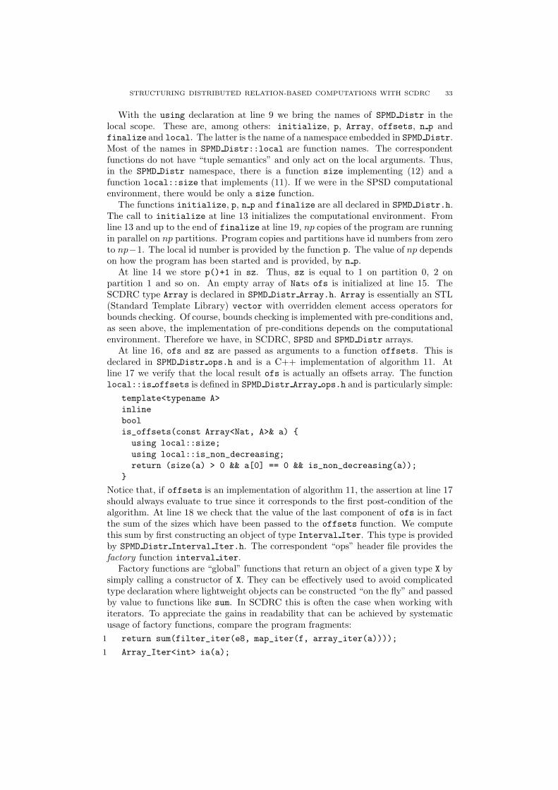
STRUCTURING DISTRIBUTED RELATION-BASED COMPUTATIONS WITH SCDRC 33
With the using declaration at line 9 we bring the names of SPMD Distr in thelocal scope. These are, among others: initialize, p, Array, offsets, n p andfinalize and local. The latter is the name of a namespace embedded in SPMD Distr.Most of the names in SPMD Distr::local are function names. The correspondentfunctions do not have “tuple semantics” and only act on the local arguments. Thus,in the SPMD Distr namespace, there is a function size implementing (12) and afunction local::size that implements (11). If we were in the SPSD computationalenvironment, there would be only a size function.
The functions initialize, p, n p and finalize are all declared in SPMD Distr.h.The call to initialize at line 13 initializes the computational environment. Fromline 13 and up to the end of finalize at line 19, np copies of the program are runningin parallel on np partitions. Program copies and partitions have id numbers from zeroto np−1. The local id number is provided by the function p. The value of np dependson how the program has been started and is provided, by n p.
At line 14 we store p()+1 in sz. Thus, sz is equal to 1 on partition 0, 2 onpartition 1 and so on. An empty array of Nats ofs is initialized at line 15. TheSCDRC type Array is declared in SPMD Distr Array.h. Array is essentially an STL(Standard Template Library) vector with overridden element access operators forbounds checking. Of course, bounds checking is implemented with pre-conditions and,as seen above, the implementation of pre-conditions depends on the computationalenvironment. Therefore we have, in SCDRC, SPSD and SPMD Distr arrays.
At line 16, ofs and sz are passed as arguments to a function offsets. This isdeclared in SPMD Distr ops.h and is a C++ implementation of algorithm 11. Atline 17 we verify that the local result ofs is actually an offsets array. The functionlocal::is offsets is defined in SPMD Distr Array ops.h and is particularly simple:
template<typename A>
inline
bool
is_offsets(const Array<Nat, A>& a) {
using local::size;
using local::is_non_decreasing;
return (size(a) > 0 && a[0] == 0 && is_non_decreasing(a));
}
Notice that, if offsets is an implementation of algorithm 11, the assertion at line 17should always evaluate to true since it corresponds to the first post-condition of thealgorithm. At line 18 we check that the value of the last component of ofs is in factthe sum of the sizes which have been passed to the offsets function. We computethis sum by first constructing an object of type Interval Iter. This type is providedby SPMD Distr Interval Iter.h. The correspondent “ops” header file provides thefactory function interval iter.
Factory functions are “global” functions that return an object of a given type X bysimply calling a constructor of X. They can be effectively used to avoid complicatedtype declaration where lightweight objects can be constructed “on the fly” and passedby value to functions like sum. In SCDRC this is often the case when working withiterators. To appreciate the gains in readability that can be achieved by systematicusage of factory functions, compare the program fragments:
1 return sum(filter_iter(e8, map_iter(f, array_iter(a))));
1 Array_Iter<int> ia(a);

34 N. BOTTA, C. IONESCU, C. LINSTEAD, R. KLEIN
2 Map_Iter<F, Array_Iter<Nat> > ifa(f, ia);
3 Filter_Iter<Eq, Map_Iter<F, Array_Iter<int> > > iffa(e8, ifa);
4 return sum(iffa);
1 return sum(Filter_Iter<Eq, Map_Iter<F, Array_Iter<int> > >
2 (e8, Map_Iter<F, Array_Iter<int> >
3 (f, Array_Iter<int>(a))));
While the first fragment is both terse and readable the same can hardly be saidof the other two15. The interval iter factory function takes a natural number nand constructs an object of type Interval Iter. Iterator objects can be advancedwith a next command, queried with is end and dereferenced with the standardstar operator. sum is a generic function that adds the values visited by its itera-tor argument to the value of an initial default argument. sum is implemented inSPMD Distr Iter ops.h:
template<class Iter>
inline
typename Iter::value_type
sum(Iter iter, typename Iter::value_type initial = 0) {
using local::begin;
using local::is_end;
using local::next;
typename Iter::value_type result = initial;
begin(iter);
while(!is_end(iter)) {
result += *iter;
next(iter);
}
return result;
}
4.2. Components, files, directories. While the two computational environmentssupported by SCDRC are implemented through C++ namespaces, most softwarecomponents are implemented as classes or collections of functions.
In SCDRC names for variables, functions, namespaces, classes, files and directories,single words are separated by underscores. Variable, function and directory names arewritten in lower case like in is non decreasing. In names of namespaces and classes,the first character of single words starts in uppercase like in Nat. The other charactersare usually written in lowercase. Exceptions are class and namespace names whichcontain acronyms. They are written as in CRS Rel where CRS means “compact rowstorage”.
As explained above, most SCDRC names are embedded either in the SPSD or in theSPMD Distr namespace. As you can see from the code examples, the namespace nameappears as a prefix of both file and of the directory names. Thus, a relation basedon a compact row storage representation is implemented, in the SPSD computationalenvironment, in the class SPSD::CRS Rel. This is declared in the file SPSD CRS Rel.h
which is found in the spsd relation/src/ directory.
15We are thankful to Dr. Andreas Priesnitz for suggesting the usage of factory functions inSCDRC.
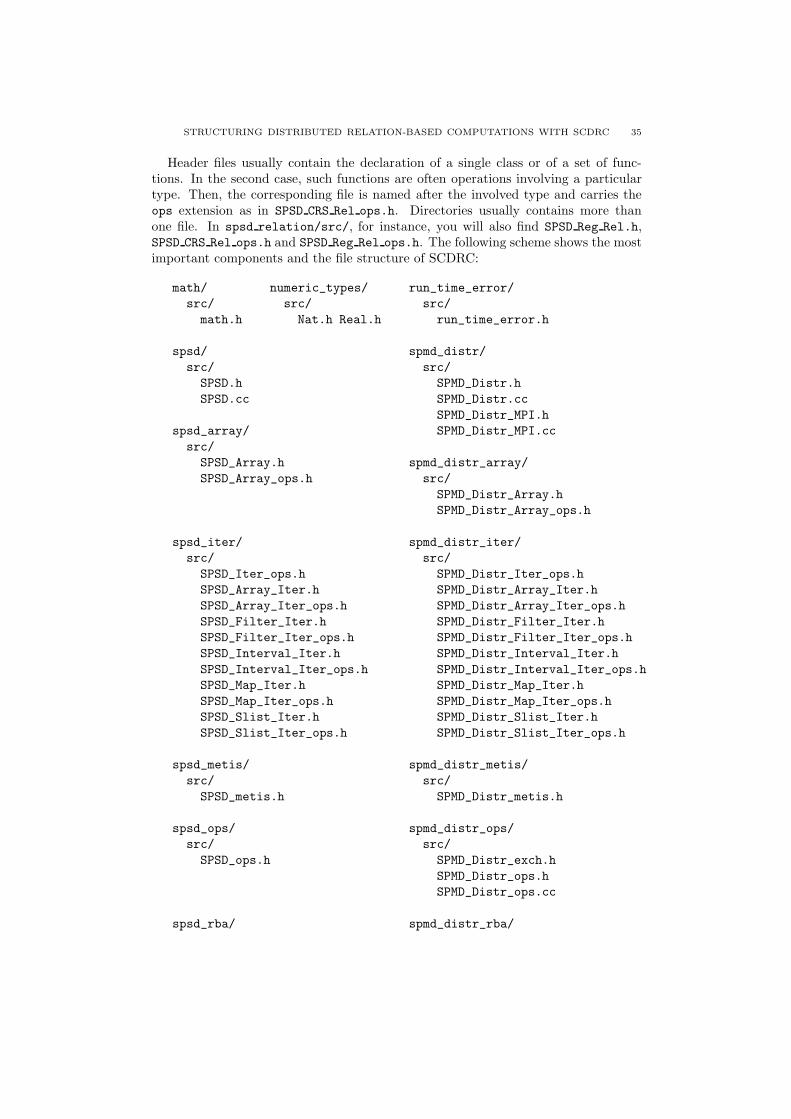
STRUCTURING DISTRIBUTED RELATION-BASED COMPUTATIONS WITH SCDRC 35
Header files usually contain the declaration of a single class or of a set of func-tions. In the second case, such functions are often operations involving a particulartype. Then, the corresponding file is named after the involved type and carries theops extension as in SPSD CRS Rel ops.h. Directories usually contains more thanone file. In spsd relation/src/, for instance, you will also find SPSD Reg Rel.h,SPSD CRS Rel ops.h and SPSD Reg Rel ops.h. The following scheme shows the mostimportant components and the file structure of SCDRC:
math/ numeric_types/ run_time_error/
src/ src/ src/
math.h Nat.h Real.h run_time_error.h
spsd/ spmd_distr/
src/ src/
SPSD.h SPMD_Distr.h
SPSD.cc SPMD_Distr.cc
SPMD_Distr_MPI.h
spsd_array/ SPMD_Distr_MPI.cc
src/
SPSD_Array.h spmd_distr_array/
SPSD_Array_ops.h src/
SPMD_Distr_Array.h
SPMD_Distr_Array_ops.h
spsd_iter/ spmd_distr_iter/
src/ src/
SPSD_Iter_ops.h SPMD_Distr_Iter_ops.h
SPSD_Array_Iter.h SPMD_Distr_Array_Iter.h
SPSD_Array_Iter_ops.h SPMD_Distr_Array_Iter_ops.h
SPSD_Filter_Iter.h SPMD_Distr_Filter_Iter.h
SPSD_Filter_Iter_ops.h SPMD_Distr_Filter_Iter_ops.h
SPSD_Interval_Iter.h SPMD_Distr_Interval_Iter.h
SPSD_Interval_Iter_ops.h SPMD_Distr_Interval_Iter_ops.h
SPSD_Map_Iter.h SPMD_Distr_Map_Iter.h
SPSD_Map_Iter_ops.h SPMD_Distr_Map_Iter_ops.h
SPSD_Slist_Iter.h SPMD_Distr_Slist_Iter.h
SPSD_Slist_Iter_ops.h SPMD_Distr_Slist_Iter_ops.h
spsd_metis/ spmd_distr_metis/
src/ src/
SPSD_metis.h SPMD_Distr_metis.h
spsd_ops/ spmd_distr_ops/
src/ src/
SPSD_ops.h SPMD_Distr_exch.h
SPMD_Distr_ops.h
SPMD_Distr_ops.cc
spsd_rba/ spmd_distr_rba/
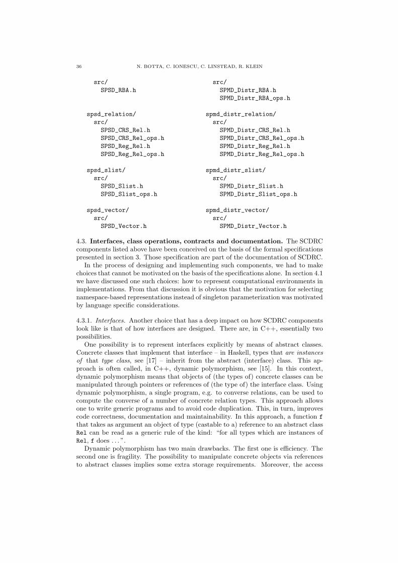
36 N. BOTTA, C. IONESCU, C. LINSTEAD, R. KLEIN
src/ src/
SPSD_RBA.h SPMD_Distr_RBA.h
SPMD_Distr_RBA_ops.h
spsd_relation/ spmd_distr_relation/
src/ src/
SPSD_CRS_Rel.h SPMD_Distr_CRS_Rel.h
SPSD_CRS_Rel_ops.h SPMD_Distr_CRS_Rel_ops.h
SPSD_Reg_Rel.h SPMD_Distr_Reg_Rel.h
SPSD_Reg_Rel_ops.h SPMD_Distr_Reg_Rel_ops.h
spsd_slist/ spmd_distr_slist/
src/ src/
SPSD_Slist.h SPMD_Distr_Slist.h
SPSD_Slist_ops.h SPMD_Distr_Slist_ops.h
spsd_vector/ spmd_distr_vector/
src/ src/
SPSD_Vector.h SPMD_Distr_Vector.h
4.3. Interfaces, class operations, contracts and documentation. The SCDRCcomponents listed above have been conceived on the basis of the formal specificationspresented in section 3. Those specification are part of the documentation of SCDRC.
In the process of designing and implementing such components, we had to makechoices that cannot be motivated on the basis of the specifications alone. In section 4.1we have discussed one such choices: how to represent computational environments inimplementations. From that discussion it is obvious that the motivation for selectingnamespace-based representations instead of singleton parameterization was motivatedby language specific considerations.
4.3.1. Interfaces. Another choice that has a deep impact on how SCDRC componentslook like is that of how interfaces are designed. There are, in C++, essentially twopossibilities.
One possibility is to represent interfaces explicitly by means of abstract classes.Concrete classes that implement that interface – in Haskell, types that are instances
of that type class, see [17] – inherit from the abstract (interface) class. This ap-proach is often called, in C++, dynamic polymorphism, see [15]. In this context,dynamic polymorphism means that objects of (the types of) concrete classes can bemanipulated through pointers or references of (the type of) the interface class. Usingdynamic polymorphism, a single program, e.g. to converse relations, can be used tocompute the converse of a number of concrete relation types. This approach allowsone to write generic programs and to avoid code duplication. This, in turn, improvescode correctness, documentation and maintainability. In this approach, a function f
that takes as argument an object of type (castable to a) reference to an abstract classRel can be read as a generic rule of the kind: “for all types which are instances ofRel, f does . . . ”.
Dynamic polymorphism has two main drawbacks. The first one is efficiency. Thesecond one is fragility. The possibility to manipulate concrete objects via referencesto abstract classes implies some extra storage requirements. Moreover, the access

STRUCTURING DISTRIBUTED RELATION-BASED COMPUTATIONS WITH SCDRC 37
to concrete objects necessarily takes place via a (virtual) pointer (table). This facttogether with limitation in compiler implementation effectively prevent inlining offunction calls. Extra storage and potentially slower access are negligible if the datastructures and the function call they affect are not atomic. Otherwise they are unac-ceptable. In our examples it would be unacceptable if, in a concrete implementationof a relation, the access to the indexes which are in relation with a given source indexwould take place via virtual pointer table.
The second drawback of dynamic polymorphism is that it leads to deep and possiblystiff class hierarchies. It also tends to lead to “fat” interfaces if multiple inheritanceis not systematically used. Systematic use of multiple inheritance is not, in turn,without problems, see [15].
Another possibility of representing interfaces in C++ is implicitly by means ofparameterization. This approach is called static (or compile-time) polymorphism. Inthis approach, any parameterized data structure implicitly defines a set of require-ments. For instance, the template function sum listed at page 31 implicitly definesthe following set of requirements for the type Iter of argument object:
(1) Iter must export the type value type.(2) A void function local::begin must be defined for objects of type Iter.(3) A function local::is end of type castable to boolmust be defined for objects
of type Iter.(4) A void function local::next must be defined for objects of type Iter.(5) A (dereferencing) operator* of type Iter::value type must be defined for
objects of type Iter.(6) operator+= must be defined for objects of type Iter::value type.
The above set of requirement could be interpreted as a refinement of an iteratorconcept in the STL sense. In general, however, sets of requirements implicitly definedby parameterized data structures cannot be easily re-conducted to useful concepts.Implicit interfaces tend to reflect more the way types are actually used than theconcepts they represent.
Implicit interfaces are more efficient and more flexible than explicit ones but theyalso have serious drawbacks. Some drawbacks are of practical nature and reflect thestate of the art in C++ compiler technology: error messages after failures in instanti-ations of heavily parameterized data structures are known for their poor readability.Other drawbacks are typical of the C++ implementation of templates: constrainedgenericity – expressing conditions like “for all types Iter such that . . . ” – is notdirectly supported in C++. Complex schemes for mimicking “type-class instance re-lationships” with static polymorphism in C++ have been proposed, among other, byBarton-Nackman [2] and Kothari and Sulzmann [13]. A more systematic approach isproposed in [16].
In SCDRC, all interfaces are represented statically and are therefore implicit. Wehave tried to document the intended usage of parameterizes data structures withcareful choices of template argument (type) names. The above definition of sum, forinstance, suggests that the first argument is expected to be an iterator. Of course,every type fulfilling the requirements 1-6 can be used as an argument of sum. We havenot been able to systematically apply Barton-Nackman or “enable if”-like approachesto constrain generic template parameters in SCDRC.

38 N. BOTTA, C. IONESCU, C. LINSTEAD, R. KLEIN
4.3.2. Class operations. For a given SCDRC type, a certain number of operations aredeclared in the corresponding ops files. Some operations are implemented for almostall SCDRC types. These are those operations that correspond to the type’s memberfunctions and output operations. Examples of operations corresponding to a type’smember functions are the already seen factory functions. They correspond to calls ofa type’s constructor. The map iter function used above, for instance, is defined asfollows:
template<class Fun, class Forward_Iter>
inline
Map_Iter<Fun, Forward_Iter>
map_iter(const Fun& f, const Forward_Iter iter) {
return Map_Iter<Fun, Forward_Iter>(f, iter);
}
Other standard functions corresponding to a type’s member functions are size,is empty, begin, end for arrays and lists and is end, next for iterators. A ver-sion of operator<< to output an object’s value is implemented for almost all SCDRCtypes. Notice that the names standard functions corresponding to some type’s mem-ber functions are necessarily heavily overloaded. Of course, heavily overloaded namesnegatively affect compile time. On the other hand, they allow to achieve a higheruniformity of notation than the more conventional mixture of member and globalfunctions. A comparison of the following code fragments shows that uniformity ofnotation can, in fact, significantly improve readability:
REQUIRE(target_size(t) <= back(offsets(source_size(s))));
REQUIRE(t.target_size() <= offsets(s.source_size()).back());
4.3.3. pre- and post-conditions and documentation. An important aspect of the designof SCDRC is the systematic usage of contracts as a documentation element. Consider,for instance, the following code fragment:
template<typename A>
inline
Array<Nat>
invert_permutation(const Array<Nat, A>& p) {
using local::require;
using local::ran_size;
using local::source_size;
using local::is_in_normal_form;
using local::compose;
using local::ensure;
REQUIRE(ran_size(p) == source_size(p));
REQUIRE(is_in_normal_form(p));
const Nat sz = source_size(p);
Array<Nat> result(sz);
for(Nat i = 0; i < sz; i++)
result[p[i]] = i;
ENSURE(compose(result, p) == id(sz));
ENSURE(compose(p, result) == id(sz));
return result;
}

STRUCTURING DISTRIBUTED RELATION-BASED COMPUTATIONS WITH SCDRC 39
The function invert permutation takes an array of natural numbers p and returnsan array of natural number result. p is understood to represent a permutation of[ 0 . . . size(p) ). Therefore the first pre-condition of invert permutation requires thesize of the range of p to coincide with the size of p16. The second pre-conditionrequires p to be in normal form. The query function is in normal form is declaredas follows:
template<class A>
inline
bool
is_in_normal_form(const Array<Nat, A>& a) /*{
using local::is_empty;
using local::min_max_elem;
using local::ran_size;
using local::target_size;
using local::ensure;
...
ENSURE(result == (ran_size(a) == target_size(a)));
return result;
}*/
The post-condition of is in normal form shows that the pre-conditions ofinvert permutation actually require:
target size(p) == ran size(p) == source size(p)
For non empty arrays of natural numbers, the size of the target is defined to be equalto one plus the maximal element of the array. Thus, the first equality implies that p issurjective on [ 0 . . .max elem(p) ). The second equality guarantees that p is bijective:if there were distinct indexes i and j in [ 0 . . .source size(p) ) with p(i) == p(j),the size of the range of p could be, at most, equal to source size(p) − 1. Thus,the pre-conditions of invert permutation require p to be a permutation. The post-conditions require the result of invert permutation to be the inverse permutationof p: composition of result with p (and of p with result) shall yield the identity.The SCDRC function id is another example of a factory function.
The discussion above shows that consistent usage of contracts and sensible nam-ing schemes can significantly improve code understandability and documentation. Ofcourse, contracts cannot, in general, express full problem specifications and for manySCDRC we have not been able to derive suitably implementable post-conditions.Contracts and pre-conditions in particular, however, can be extremely useful in docu-menting the intended usage of functions. As an example we list the pre-conditions onthe “in” arguments of partition recursive, a subset of the the SCDRC interface toMetis for partitioning the source of symmetric, anti-reflexive relations with minimaledge cut:
template<class Rel>
void
partition_recursive(Array<Nat>& part,
Nat& n_cuts,
16In SCDRC, size and source size are, for arrays, the same function. Both return the length
(the number of elements) of the array. We use size and source size for container and functionarguments, respectively.
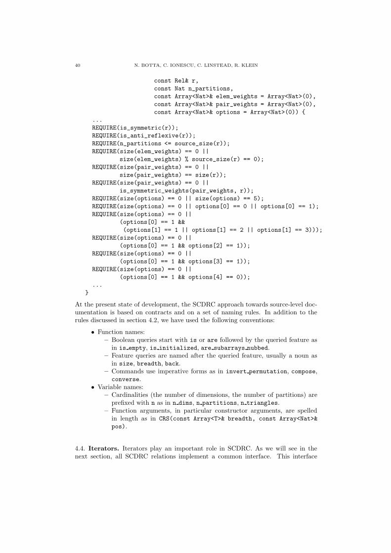
40 N. BOTTA, C. IONESCU, C. LINSTEAD, R. KLEIN
const Rel& r,
const Nat n_partitions,
const Array<Nat>& elem_weights = Array<Nat>(0),
const Array<Nat>& pair_weights = Array<Nat>(0),
const Array<Nat>& options = Array<Nat>(0)) {
...
REQUIRE(is_symmetric(r));
REQUIRE(is_anti_reflexive(r));
REQUIRE(n_partitions <= source_size(r));
REQUIRE(size(elem_weights) == 0 ||
size(elem_weights) % source_size(r) == 0);
REQUIRE(size(pair_weights) == 0 ||
size(pair_weights) == size(r));
REQUIRE(size(pair_weights) == 0 ||
is_symmetric_weights(pair_weights, r));
REQUIRE(size(options) == 0 || size(options) == 5);
REQUIRE(size(options) == 0 || options[0] == 0 || options[0] == 1);
REQUIRE(size(options) == 0 ||
(options[0] == 1 &&
(options[1] == 1 || options[1] == 2 || options[1] == 3)));
REQUIRE(size(options) == 0 ||
(options[0] == 1 && options[2] == 1));
REQUIRE(size(options) == 0 ||
(options[0] == 1 && options[3] == 1));
REQUIRE(size(options) == 0 ||
(options[0] == 1 && options[4] == 0));
...
}
At the present state of development, the SCDRC approach towards source-level doc-umentation is based on contracts and on a set of naming rules. In addition to therules discussed in section 4.2, we have used the following conventions:
• Function names:– Boolean queries start with is or are followed by the queried feature as
in is empty, is initialized, are subarrays nubbed.– Feature queries are named after the queried feature, usually a noun as
in size, breadth, back.– Commands use imperative forms as in invert permutation, compose,
converse.• Variable names:
– Cardinalities (the number of dimensions, the number of partitions) areprefixed with n as in n dims, n partitions, n triangles.
– Function arguments, in particular constructor arguments, are spelledin length as in CRS(const Array<T>& breadth, const Array<Nat>&
pos).
4.4. Iterators. Iterators play an important role in SCDRC. As we will see in thenext section, all SCDRC relations implement a common interface. This interface
STRUCTURING DISTRIBUTED RELATION-BASED COMPUTATIONS WITH SCDRC 41
essentially consists of five iterators. Examples of SCDRC functions acting on iteratorsor producing iterators are the factory functions discussed in section 4.1.
As in the standard template library, SCDRC iterators act as a link between genericalgorithms and a variety of traversable data structures. However, SCDRC iteratorsare different from STL iterators in many ways, being more similar to Boost ranges.In SCDRC, a type Iter represents an iterator if:
• Iter exports the type value type. This means that Iter contains a pub-lic typedef declaration where value type appears as the second argument oftypedef as in typedef Nat value type; in the SCDRC class Interval Iter.• Iters can be dereferenced with operator*.• Iters can be queried with is end.• Iters can be incremented with next.
Because the state of SCDRC iterators can be queried with is end, traversable datastructures can be visited with a single iterator and there is no need to operate with“begin” and “end” iterator pairs as in STL. A second important difference betweenSTL and SCDRC iterators is that SCDRC iterators can be used to represent lazilyevaluated computational rules. Consider, for instance, the program fragment:
Map_Iter<F, Array_Iter<Nat> > ifa(f, ia);
Here ifa is an object of type Map Iter. It is constructed with a function f of typeF and with an iterator over arrays of natural numbers. We can step through anddereference ifa with the iterator interface, for instance as in:
while(!is_end(ifa)) {
if(is_odd(*ia))
cout << *ifa << endl;
next(ia);
next(ifa);
}
VERIFY(is_end(ia));
The program fragment prints the values of f at the odd elements of the array iteratedby ia. The evaluation of f takes place where ifa is dereferenced. This means thatifa represents the mapping of f on ia lazily: if the natural numbers visited by ia
are all even, f is never evaluated.A small set of basic iterator classes is implemented, in SCDRC, in spsd iter and
spmd distr iter: Interval Iter, Array Iter, Slist Iter, Map Iter and Filter Iter.These operators extend the above interface with the command begin, the query size
and with the random access operator operator[].
4.5. Relations. As explained in 4.3.1, SCDRC interfaces are implicit. As for itera-tors, there is no abstract class from which concrete relation classes are derived andwe use the expression relation interface to denote a set of functionalities that anyconcrete SCDRC relation Rel has to implement. These are:
• Public definitions of five nested iterator classes:– Lambdas Iter
– Lambda Sizes Iter
– Lambda Offsets Iter
– Graph Ran Iter
– Graph Dom Iter
Each class implements the basic iterator functionalities of the previous section.
42 N. BOTTA, C. IONESCU, C. LINSTEAD, R. KLEIN
• Public definition of five void constant Rel member functions:lambdas, lambda sizes, lambda offsets, graph ran and graph dom. Thereturn types of these functions correspond with the types of the nested classes.• Definition of five factory functions lambdas, lambda sizes, lambda offsets,graph ran and graph dom. These functions take (constant references) Rel
arguments and return types correspondent to those of the nested classes.They simply call the correspondent member function on the argument. Forinstance, lambdas is defined as follows:
inline
Rel::Lambdas_Iter
lambdas(const Rel& r) {
return r.lambdas();
}
In Lambdas Iter, the value of value type is Array Iter<const Nat>: this is thetype of the objects which are obtained by dereferencing the output of lambdas. If ris a SCDRC object representing some relation R, lambdas(r)[j] returns an iteratorover the indexes of R(j).
In the other nested classes, the value of value type is Nat. lambda sizes(r)[j]
and lambda offsets(r)[j] provide access to the size and to the offset associated toR(j). For j in [ 0 . . .source size(r) ), they fulfill:
size(lambda sizes(r)) == source size(r)
∧size(lambda offsets(r)) == source size(r) + 1
∧lambda offsets(r)[0] == 0
∧lambda offsets(r)[j+ 1] == lambda offsets(r)[j] + lambda sizes(r)[j]
The iterators returned by graph ran and by graph dom allow traversing a relation as aset of pairs. This is particularly useful in the implementation of relational operationslike converse and compose.
At the present stage, SCDRC provides two data structures for relations: CRS Rel
and Reg Rel<n>. The first class is useful for irregular relations i.e. for relationsfor which the size of R(j) is not constant. The second class is useful for regular
relations such as the vertex-triangle relation of our example. The template Nat valuen represents the size of the R(j).
Both CRS Rel and Reg Rel<n> use, internally, arrays of Nats to store the elementsof R(j) and guarantee access to these elements in asymptotically constant time. Asmentioned in section 2, efficient access to R(j) is crucial for the implementation ofrelation-based algorithms.
In many important applications, however, implementations of R(j) in terms ofarrays are sub-optimal. For neighborhood relations on structured grids, for instance,functions like R(j) can be written in terms of simple analytical expression. In this case,it would be computationally inefficient to represent such relations with Reg Rel<n>sor with CRS Rels. Using the examples of CRS Rel and Reg Rel<n>, it is easy to extendSCDRC with lightweight types which are optimized for particular classes of relations.
STRUCTURING DISTRIBUTED RELATION-BASED COMPUTATIONS WITH SCDRC 43
As far as the new types implement the interface described above, they can be used inrelation-based computations in the same way as CRS Rel and Reg Rel<n>. We planto provide such extensions upon user’s demand.
4.6. Relation-based algorithms. In section 2 we have introduced relation-basedalgorithms as generic computational rules defined in terms of a relation R, of a func-tions f taking values in the target of R and of a “reduction” operator h. In section 4we have seen that, in order to apply parallel SPMD relation-based algorithms, auxil-iary data structures and functionalities are in general needed. These can be describedin terms of suitable exchange and access tables and in terms of functionalities tocomplete local array-based partial representations of f .
In SCDRC, relation-based algorithms are implemented as specializations of a generictype RBA:
template<class H,
class F,
class R,
Nat h_arity = H::arity,
Nat f_arity = F::arity>
class
RBA;
Objects of type RBA can be easily constructed by passing objects of type H, F and R
to the RBA constructor as in
RBA<H, F, R> tca(triangle_center,
vertex_coordinates(tri),
vertex_triangle(tri));
H is, in general, a user-defined type. It is required to export the type return type,the constant Nat value arity and to implement a generic function call operatoroperator(). For the case arity == 1, operator() is required to have the followingsignature:
template<class Random_Access_Data>
return_type
operator()(Random_Access_Data& x) const;
In most practical cases, H is a user defined wrapper of some specific, problem depen-dent computational rule. In the example given above, for instance, H represents a rulefor computing the triangle centers. As mentioned in section 2, this rule depends onapplication specific aspects like the kind of triangles (plane, spherical), the coordinatesystem associated with the triangle vertexes etc. In our triangle centers example, forinstance, H is defined as follows:
typedef Triangle_Area<Coordinate_System> H;
template<class Coordinate_System>
class Triangle_Center {
public:
typedef Vector<Real, Coordinate_System::n_crds> return_type;
static const Nat arity = 1;
template<class Random_Access_Data>
Vector<Real, Coordinate_System::n_crds>
operator()(Random_Access_Data& x) const {
44 N. BOTTA, C. IONESCU, C. LINSTEAD, R. KLEIN
return Coordinate_System::triangle_center(x[0], x[1], x[2]);
}
};
In many practical cases, F is an array of a type matching the type of the argumentsof the specific rule wrapped by H, in our example triangle center. However, F
could be an RBA itself. This allows relation-based algorithms to be composed toexpress complex computational patterns. The type R is an SCDRC relation. Asdiscussed above, SCDRC provides, at the present stage, two relation types: CRS Rel
and Reg Rel<n>.In the SPSD computational environment, relation-based algorithms can be evalu-
ated right after construction. The triangle center algorithm object tca of out example,for instance, could be evaluated on the triangles of tri with the simple loop:
for(Nat i = 0; i < source_size(vertex_triangle(tri)); i++)
cout << tca(i) << endl;
In the SPMD distributed computational environment, and for the case in which F isan array, the auxiliary access and exchange tables have to be computed and the localarrays f have to be completed before relation based algorithms can be evaluated. TheSPMD distributed computational environment supports these computations with twofunctions. They can be called with relation-based algorithm arguments as follows:
init_access_exch_tables(tca);
complete_f(tca);
As discussed in section 3.3, these functions allow users to set up parallel computationsof distributed relation-based algorithms without having to care about message passinglevel communication and related synchronization, mutual exclusion, deadlock or racecondition problems. At the same time, init access exch tables and complete f
support the optimization of computational procedures in which complete f has to becalled at each step of some iteration, init access exch tables, however, only onceat the beginning of the iteration. In scientific computing, such iterative proceduresare found, e.g. in the numerical integration of (partial) differential equations, in linearalgebra and in the solution of optimization problems.
4.7. Communication primitives, exchange and MPI interface. In the nextand last section of this report, we show how to setup a parallel computation ofthe centers of the triangles of a distributed triangulation. We are going to usesome of the SCDRC data structures discusses in this section, functionalities likeinit access exch tables and complete f and primitives for redistributing distributedarrays and relations.
As mentioned in section 3, all SCDRC functionalities that require data communi-cation between partitions have been designed on the top of a single communicationprimitive called exchange. An implementation of exchange is provided, in the SPMDdistributed computational environment by the function SPMD Distr::exch. Thisfunction is implemented, internally, in terms of the MPI primitive MPI Alltoallv.This is one of the few MPI functionalities used by SCDRC. In SCDRC, most MPIentities are accessed via a small interface. This is implemented as a MPI namespaceembedded in SPMD Distr. SPMD Distr::MPI contains:
• The type Comm (MPI Comm).• The constant values:
– INT (MPI INT).
STRUCTURING DISTRIBUTED RELATION-BASED COMPUTATIONS WITH SCDRC 45
– CHAR (MPI CHAR).– communicator (MPI COMM WORLD).
• The functions:– initialize, implemented in terms of MPI Init.– is initialized, implemented in terms of MPI Initialized.– finalize, implemented in terms of MPI Finalize.– is finalized, implemented in terms of MPI Finalized.– get rank, implemented in terms of MPI Comm rank.– get size, implemented in terms of MPI Comm size.
Other MPI entities used in SCDRC are the already mentioned MPI Alltoallv andMPI Abort and MPI Allgather. MPI Alltoallv is used only in the implementation ofexch. The other two MPI primitives are used only in the implementation of contractsin the SPMD distributed environment. Thus, the dependency of SCDRC on MPI islimited to a few primitives and confined to very few files.
5. Preliminary results, outlook
In this section we show how SCDRC can be used to set up a parallel computationof the center of the areas of a triangulation and present some preliminary results. Weclose this report with an outlook on future activities.
5.1. Center of area computations. In this example we set up a parallel computa-tion of the center of the areas of a triangulation. The computation is embedded in atime stepping procedure. On each partition and at each iteration step, the coordinatesof the vertexes of the triangulation are displaced according to a simple rule and a newcenter is computed. The computation of the center is based on two relation-basedalgorithms, one for computing the centers and one for computing the areas of thetriangles. The coordinates of the center of the triangulation and of its total area areaccumulated in local variables c and a. At the end of the iteration, the average centercoordinates and the average areas are collected, together with simple computationmetrics, on partition zero. Here the average center is computed and the results aresent to the standard output.
Beside the SCDRC functionalities discussed in section 4, we use simple componentsfor representing surface triangulations and basic rules for geometrical computationsin a three-dimensional Cartesian coordinate system. These components are not partof SCDRC. The type Tri, in particular, just wraps a vertex-triangle relation and avertex coordinates array in a data structure. For this data structure, basic input-output functionalities are provided in different data formats, e.g. for visualization.
In setting up the computation, we assume, as discussed at the end of the specifi-cation of problem 2 in section 3, that the triangulation, together with correspondentoffsets for the vertex coordinates and for the vertex-triangle relation, are stored infiles which are given as arguments on the command line. This is consistent withsteps 1-3 of page 18. This means that, in a pre-processing step, we have alreadycomputed a partitioning of the triangles and of the vertexes of the triangulation andwe have renumbered the original vertex-triangle relation and the vertex coordinatesarray accordingly. The output of these computations, a “new” triangulation and thecorrespondent offsets arrays, is the input of our example. We interleave the listing ofthe program with remarks.
1 #include <numeric_types/src_cc/Nat.h>
46 N. BOTTA, C. IONESCU, C. LINSTEAD, R. KLEIN
2 #include <run_time_error/src_cc/run_time_error.h>
3 #include <spmd_distr/src_cc/SPMD_Distr.h>
4 #include <spmd_distr_ops/src_cc/SPMD_Distr_ops.h>
5 #include <spmd_distr_array/src_cc/SPMD_Distr_Array.h>
6 #include <spmd_distr_array/src_cc/SPMD_Distr_Array_ops.h>
7 #include <spmd_distr_relation/src_cc/SPMD_Distr_Reg_Rel.h>
8 #include <spmd_distr_relation/src_cc/SPMD_Distr_Reg_Rel_ops.h>
9 #include <spmd_distr_iter/src_cc/SPMD_Distr_Interval_Iter.h>
10 #include <spmd_distr_iter/src_cc/SPMD_Distr_Interval_Iter_ops.h>
11 #include <spmd_distr_iter/src_cc/SPMD_Distr_Map_Iter.h>
12 #include <spmd_distr_iter/src_cc/SPMD_Distr_Map_Iter_ops.h>
13 #include <spmd_distr_rba/src_cc/SPMD_Distr_RBA.h>
14 #include <spmd_distr_rba/src_cc/SPMD_Distr_RBA_ops.h>
At lines 1-2, we include the header files for natural numbers and contracts. These donot depend on the computational environment. Subsequently, we include the SPMDdistributed computational environment, its operations, distributed arrays, relations,iterators and relation-based algorithms with the respective operations.
15 #include <spmd_distr_geometry/src_cc/SPMD_Distr_Rect_Coord_Sys.h>
16 #include <spmd_distr_triangulation/src_cc/SPMD_Distr_Tri.h>
17 #include <spmd_distr_triangulation/src_cc/SPMD_Distr_Tri_ops.h>
18 #include <spmd_distr_geometry/src_cc/SPMD_Distr_Triangle.h>
19 #include <spmd_distr_io_ascii/src_cc/SPMD_Distr_io_ascii.h>
20 #include <fstream>
21 #include <iostream>
22 #include <string>
23
24 using namespace SPMD_Distr;
25 using namespace std;
26 using local::operator<<;
Next, we include non-SCDRC components for geometrical rules, triangulations andIO in ASCII format. This is the format in which the triangulation and the offsetarrays are stored in the input files. At line 24, we bring all the names of the SPMDdistributed computational environment in the global scope. At line 26, we injectlocal::operator<< in the global scope. As mentioned earlier, most SCDRC datastructures can be processed by operator<<. At the present, we have not implementedany version of operator<<with “tuple-semantics”. The implemented operator<< acton local data and are therefore embedded, in the SPMD distributed computationalenvironment, in the local namespace. Since there is no ambiguity in the usage ofthese operators, we make them available in the global scope.
27 int
28 main(int argc, char** argv) {
29
30 if(argc < 4) {
31 cerr << "Usage: "
32 << argv[0]
33 << " tri vofs tofs"
34 << endl;
35 exit(0);
STRUCTURING DISTRIBUTED RELATION-BASED COMPUTATIONS WITH SCDRC 47
36 }
37
38 initialize(argc, argv);
At line 38, after the number of command line arguments check, we issue the firstSPMD function call: initialize starts the SPMD distributed computational envi-ronment. From line 38 and up to the call to finalize at line 135, n p() copies ofthe program are running in parallel on n p() partitions.
39 Reg_Rel<3> vt;
40 Array<Vector<Real, 3> > vx;
41 Array<Nat> vtofs(n_p() + 1, 0);
42 Array<Nat> vxofs(n_p() + 1, 0);
43
44 if(p() == 0) {
45 typedef Rect_Coord_Sys<3> Coord_Sys;
46 typedef Tri<Coord_Sys> T;
47 T tri;
48 string tri_file = argv[1];
49 local::read_ascii(tri, tri_file);
50 vt = tri.vertex_triangle();
51 vx = tri.vertex_coordinates();
52 string vofs_file = argv[2];
53 local::read_ascii(vxofs, vofs_file);
54 string tofs_file = argv[3];
55 local::read_ascii(vtofs, tofs_file);
56 local::VERIFY(local::is_offsets(vxofs));
57 local::VERIFY(local::size(vxofs) == n_p() + 1);
58 local::VERIFY(local::target_size(vt) == local::back(vxofs));
59 local::VERIFY(local::is_offsets(vtofs));
60 local::VERIFY(local::size(vtofs) == n_p() + 1);
61 local::VERIFY(local::source_size(vt) == local::back(vtofs));
62 }
First we initialize, on each partition, an empty vertex-triangle regular relation vt, anempty array of vertex coordinates vx and trivial partitioning offsets vtofs and vxofs
for the source of vt and for the source of vx, respectively. These variables correspondto vtp, xp, ovtp and oxp of steps 1-3 of page 18.
Then, on partition 0, we initialize an empty triangulation tri in a three-dimensionalrectangular (Cartesian) coordinate system (lines 45-47), we read tri from the filegiven on the command line (lines 48-49) and we initialize vt and vx with the vertex-triangle relation and with the vertex coordinates array of tri.
At lines 52-61, we read the offsets arrays and we verify the consistency of theinput data. In particular, we check that vtofs and vxofs are indeed offsets arrays ofproper size and that they represent non-decreasing partitioning functions for vt andvx, respectively. Notice the local qualifier in front of the VERIFY macros and in theirargument expressions.
63 Reg_Rel<3> vtp;
64 redistribute_after_offsets(vtp, vt, vtofs);
65 Array<Vector<Real, 3> > vxp;
66 redistribute_after_offsets(vxp, vx, vxofs);
48 N. BOTTA, C. IONESCU, C. LINSTEAD, R. KLEIN
67 Array<Nat> ofs;
68 offsets(ofs, vxp.size());
69 typedef Rect_Coord_Sys<3> Coord_Sys;
70 typedef Triangle_Area<Coord_Sys> TA;
71 typedef Triangle_Center<Coord_Sys> TC;
72 typedef Array<Vector<Real, 3> > F;
73 typedef Reg_Rel<3> R;
74 TA triangle_area;
75 TC triangle_center;
76 RBA<TA, F, R> taa(triangle_area, vxp, vtp, ofs);
77 RBA<TC, F, R> tca(triangle_center, vxp, vtp, ofs);
At this point, we are ready to set up a parallel computation of the center of the areasof tri. We first redistribute vt and vx according to vtofs, vxofs. This is done atlines 64-67 and yields, on each partition, a new distributed vertex-triangle relationvtp and a new vertex coordinates array vxp.
Notice the usage of redistribute after offsets: this is an overloaded function(it is used, at lines 65 to redistribute a Reg Rel<3> relation and, at line 67, to redis-tribute an array) which implements the specifications of problem 2’ and 1’ of section3.3. Therefore, redistribute after offsets has “tuple-semantics” although, asexplained in section 4.1, only local data formally appear as “function” arguments.
redistribute after offsets is an example of how SCDRC supports structuringparallel computations by providing communication primitives that relieve the userfrom the burden of low-level data transferring. As explained in the introduction,however, SCDRC does not attempt to hide the underlying distributed data modelto the user. This model is visible in the offsets array arguments that “high-level”SCDRC primitives like redistribute after offsets require.
The offsets arrays vtofs and vxofs describe, on each partition, which chunks ofvt and vx have to be sent to which partition. In order to efficiently initialize therelation-based algorithms, it is useful to compute, on each partition, the offsets thatdescribe how the new distributed vertex coordinates array vxp is actually distributed.This is done at lines 67 and 68.
Lines 69 to 77 is where the relation-based algorithms taa and tca for triangleareas and centers are actually constructed. The typedefs instructions just introduceconvenient type synonyms; the RBA constructors are called in the last two lines.Notice that both taa and tac use the same “f” function vxp and the same “R” relationvtp. The “h” functions of taa and tca are triangle area and triangle center,respectively. These rules are provided by non-SCDRC components. As the exampleshows, RBAs are quite flexible generic types: users can define their own “h” functionsto construct ad hoc RBA objects.
78 init_access_exch_tables(taa);
79 init_access_exch_tables(tca);
80 const Nat n_iter = 10000;
81 const Real alpha = 0.1;
82 const Real omega = 1.0;
83 Array<Vector<Real, 3> > vx0(vxp);
84 Real a = 0.0;
85 Vector<Real, 3> c = Vector<Real, 3>(0.0);
86 for(Nat iter = 0; iter < n_iter; iter++) {
STRUCTURING DISTRIBUTED RELATION-BASED COMPUTATIONS WITH SCDRC 49
87 const Real t = 2.0 * Real_PI * Real(iter) / Real(n_iter - 1);
88 for(Nat i = 0; i < vx0.size(); i++)
89 vxp[i] = vx0[i] * (1.0 + alpha * sin(omega * t));
90 complete_f(taa);
91 complete_f(tca);
92 for(Nat j = 0; j < local::source_size(vtp); j++) {
93 const Real area = taa(j);
94 const Vector<Real, 3> center = tca(j);
95 a += area;
96 c += area * center;
97 }
98 }
99 a /= Real(n_iter);
100 c /= Real(n_iter);
Since we are in the SPMD computational environment and the “f” function of taa
and tca is represented by a distributed array, the auxiliary access and exchange tableshave to be computed and the local arrays f have to be completed before taa and tca
can actually be evaluated.The computation of the access and exchange tables is done at lines 78 and 79.
This is outside the main iteration (lines 86 to 98) because the tables only dependon the vertex-triangle relation and on the offsets of the vertex coordinate arrays. Incontrast to the vertex coordinates, the relation and the offsets do not change duringthe iteration. As explained in section 3.3, the computation of the access and exchangetable is computationally demanding and it would be very inefficient to recompute suchtables every time we need to complete the local vertex coordinates arrays.
At lines 80-82 we initialize the number of iterations n iter, the amplitude alpha
and the frequency omega. Amplitude and the frequency are used at line 89 to imposea simple periodic motion on the vertexes of the triangulation. At lines 83-85 weinitialize an auxiliary array of vertex coordinates vx0 and the variable a and c. Weuse a and c to accumulate the sums of the areas and of the centers of the triangulation.
Inside the iteration we first compute an “iteration time” t and move the vertexesof the triangulation. Then, at lines 90-91, we complete the local vertex coordinatearray with the “new” values. As for the access and exchange table computationsdiscussed above, SCDRC users are supposed to know that, at each iteration step,vertex coordinates have to be exchanged between partitions. However, SCDRC usersdo not need to know the details of which data have to be exchanged and of how thiscan be done. They simply call the SCDRC primitives init access exch tables andcomplete f. After these calls, all partitions have enough data to compute the areasand the centers of the triangles independently of each other: the loop at lines 92-97can be done in parallel. This loop is where the computational work is actually done:for each triangle, we compute the triangle area with taa and the triangle center withtca. These results are stored in the loop variables area and center. These are usedto increment a and c at lines 95 and 96. At lines 99-100, a and c are divided by thenumber of iteration thus yielding the average area and triangulation center.
135 finalize();
136 return 0;
137 }
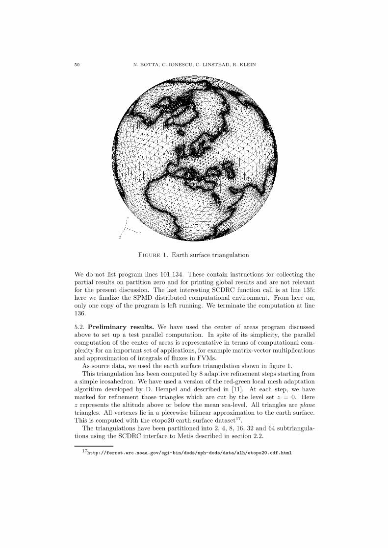
50 N. BOTTA, C. IONESCU, C. LINSTEAD, R. KLEIN
Figure 1. Earth surface triangulation
We do not list program lines 101-134. These contain instructions for collecting thepartial results on partition zero and for printing global results and are not relevantfor the present discussion. The last interesting SCDRC function call is at line 135:here we finalize the SPMD distributed computational environment. From here on,only one copy of the program is left running. We terminate the computation at line136.
5.2. Preliminary results. We have used the center of areas program discussedabove to set up a test parallel computation. In spite of its simplicity, the parallelcomputation of the center of areas is representative in terms of computational com-plexity for an important set of applications, for example matrix-vector multiplicationsand approximation of integrals of fluxes in FVMs.
As source data, we used the earth surface triangulation shown in figure 1.This triangulation has been computed by 8 adaptive refinement steps starting from
a simple icosahedron. We have used a version of the red-green local mesh adaptationalgorithm developed by D. Hempel and described in [11]. At each step, we havemarked for refinement those triangles which are cut by the level set z = 0. Herez represents the altitude above or below the mean sea-level. All triangles are plane
triangles. All vertexes lie in a piecewise bilinear approximation to the earth surface.This is computed with the etopo20 earth surface dataset17.
The triangulations have been partitioned into 2, 4, 8, 16, 32 and 64 subtriangula-tions using the SCDRC interface to Metis described in section 2.2.
17http://ferret.wrc.noaa.gov/cgi-bin/dods/nph-dods/data/alh/etopo20.cdf.html

STRUCTURING DISTRIBUTED RELATION-BASED COMPUTATIONS WITH SCDRC 51
Figure 2. Partitioning of the triangulation into 32 subpartitions.
2 part. 4 part. 8 part. 16 part. 32 part. 64 part.
total num. triangles 86750 86750 86750 86750 86750 86750min. triangles per part. 43311 21344 10527 5226 2629 1307max. triangles per part. 43439 22020 11153 5583 2794 1398
tot. comm. volume 187 406 638 1138 1745 2538min. comm. volume 77 77 56 53 34 23max. comm. volume 110 112 92 128 84 65
Table 1. Parallel triangulation center computation metrics.
Figure 2 shows the result of this partitioning into 32 subpartitions and some im-portant metrics associated with different partitionings are summarized in table 1.
In particular, the communication volume for a given partition (table 1) is definedas the number of elements (of the type of the elements of vx, Vector<Real, 3>) thatthat partition has to send in a single complete f call.
After init access exch tables has been called on a relation-based algorithm,this number and the number of partitions the data have to be sent to (the number ofcommunication peers) can be queried with a SCDRC function.
The computations have been run on an IBM p655 cluster consisting of 30 nodeswith 8 Power4 1.1GHz CPUs per node. For computations involving 8 partitions andabove, we have used a blocking factor of 8. The blocking factor specifies the way inwhich processes will be assigned to a node. For a blocking factor of 8, entire nodes

52 N. BOTTA, C. IONESCU, C. LINSTEAD, R. KLEIN
2 proc. 4 proc. 8 proc. 16 proc. 32 proc. 64 proc.
time (n = 1) 1866 944 485 321 385 784speedup 1 1.98 3.84 5.81 4.84 2.38
time (n = 10) 1854 919 466 247 144 139speedup 1 2.01 3.98 7.51 12.88 13.34
time (n = 100) 1890 976 480 241 129 67speedup 1 1.93 3.94 7.84 14.65 28.21
time (no comm.) 1878 926 458 229 114 57speedup 1 2.02 4.1 8.2 16.47 32.95
Table 2. Parallel triangulation center computation times.
are reserved for the application. For 2 or 4 tasks and a blocking factor of 2 or 4respectively, it is guaranteed that the tasks will run on the same node.
Execution times were recorded for several sets of runs and speedup values calculatedaccordingly. Each run had a fixed number of iterations (N = 100000). Speedup isdefined here as the ratio between the time taken to run on np processors relative to thetime taken with 2 processors. Times have been calculated by calling the MPI Wtime()function - which returns current wall-clock time - before and after the main executionloop. All processes are synchronized before measurements are taken by calling theMPI Barrier() function.
We also modified the code to investigate the effect of changing the ratio betweencomputation and communication costs. This was done by changing how often thecommunication was carried out during a run while keeping the number of computationsteps constant. Specifically, this was carried out by changing how often complete f
was called inside the main execution loop. Table 2 shows the execution times (inseconds) and speedup values for communication at every step (n = 1) and at every10th (n = 10) and 100th (n = 100) step and for the case of no communication (n = 0).
With the partitioning scheme described above and with no communication, weexpect the total run time to halve with each doubling of the number of processors.
Table 2 shows that this is indeed the case. As the frequency of communicationincreases, and with a greater number of processors, it can be seen that we get muchless than this ideal speedup. In the extreme case of 64 processors and communicationat every iteration (n = 1), the performance is only marginally better than when usingjust 2 processors.
We will now try to explain the results in table 2 by means of a simple computationalcost model. The time taken for a run is the sum of two components, computationtime and communication time: t = tcomp + tcomm. As can be seen from table 2computation time is inversely proportional to the number of processors being used inthe no-communication case. We expect this to hold for all communication frequencycases: tcomp = k1/np.
The communication time for N iterations is proportional to the number of commu-nication steps, i.e. N/n.
tcomm = t1 ·N
n
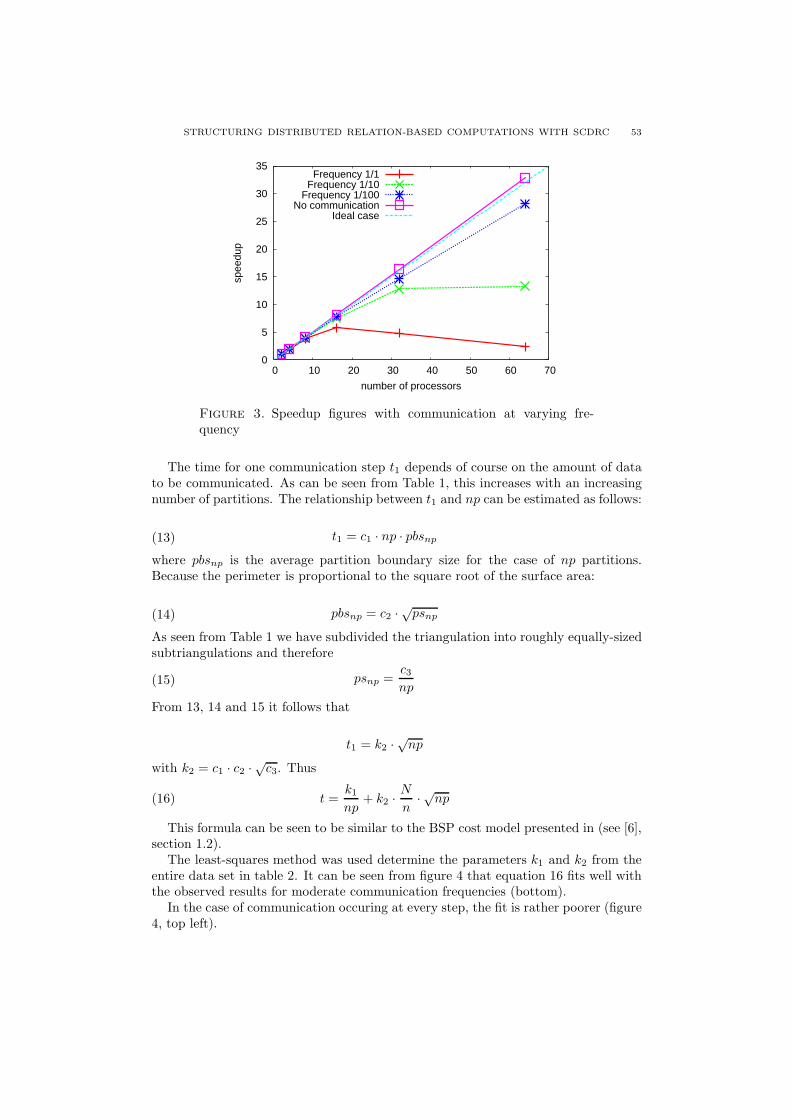
STRUCTURING DISTRIBUTED RELATION-BASED COMPUTATIONS WITH SCDRC 53
0
5
10
15
20
25
30
35
0 10 20 30 40 50 60 70
spee
dup
number of processors
Frequency 1/1Frequency 1/10
Frequency 1/100No communication
Ideal case
Figure 3. Speedup figures with communication at varying fre-quency
The time for one communication step t1 depends of course on the amount of datato be communicated. As can be seen from Table 1, this increases with an increasingnumber of partitions. The relationship between t1 and np can be estimated as follows:
t1 = c1 · np · pbsnp(13)
where pbsnp is the average partition boundary size for the case of np partitions.Because the perimeter is proportional to the square root of the surface area:
pbsnp = c2 ·√
psnp(14)
As seen from Table 1 we have subdivided the triangulation into roughly equally-sizedsubtriangulations and therefore
psnp =c3
np(15)
From 13, 14 and 15 it follows that
t1 = k2 ·√
np
with k2 = c1 · c2 ·√
c3. Thus
t =k1
np+ k2 ·
N
n· √np(16)
This formula can be seen to be similar to the BSP cost model presented in (see [6],section 1.2).
The least-squares method was used determine the parameters k1 and k2 from theentire data set in table 2. It can be seen from figure 4 that equation 16 fits well withthe observed results for moderate communication frequencies (bottom).
In the case of communication occuring at every step, the fit is rather poorer (figure4, top left).
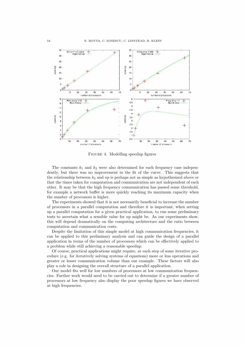
54 N. BOTTA, C. IONESCU, C. LINSTEAD, R. KLEIN
Figure 4. Modelling speedup figures
The constants k1 and k2 were also determined for each frequency case indepen-dently, but there was no improvement in the fit of the curve. This suggests thatthe relationship between k2 and np is perhaps not as simple as hypothesized above orthat the times taken for computation and communication are not independent of eachother. It may be that the high frequency communication has passed some threshold,for example a network buffer is more quickly reaching its maximum capacity whenthe number of processors is higher.
The experiments showed that it is not necessarily beneficial to increase the numberof processors in a parallel computation and therefore it is important, when settingup a parallel computation for a given practical application, to run some preliminarytests to ascertain what a sensible value for np might be. As our experiments show,this will depend dramatically on the computing architecture and the ratio betweencomputation and communication costs.
Despite the limitation of this simple model at high communication frequencies, itcan be applied to this preliminary analysis and can guide the design of a parallelapplication in terms of the number of processors which can be effectively applied toa problem while still achieving a reasonable speedup.
Of course, practical applications might require, at each step of some iterative pro-cedure (e.g. for iteratively solving systems of equations) more or less operations andgreater or lesser communication volume than our example. These factors will alsoplay a role in designing the overall structure of a parallel application.
Our model fits well for low numbers of processors at low communication frequen-cies. Further work would need to be carried out to determine if a greater number ofprocessors at low frequency also display the poor speedup figures we have observedat high frequencies.

STRUCTURING DISTRIBUTED RELATION-BASED COMPUTATIONS WITH SCDRC 55
5.3. Outlook. We have presented a prototype version of SCDRC, a small set ofsoftware components for distributed relation-based computations. As explained inthe introduction, SCDRC is a thin software layer above message passing libraries andis not meant to be directly used by applications. Applications are expected to useSCDRC indirectly via application dependent components.
The triangulation and geometry components used to write the parallel programfor computing the center of a triangulation are simple examples of an applicationdependent software layer built upon SCDRC. In fact, SCDRC has been written in theframework of a project for developing software components for distributed adaptivefinite volume computations18. In finite volume computations, relation-based algo-rithms and relation-based computations play an outstanding role.
Relation-based algorithms and relation-based computations, however, are found indifferent research areas at the core of many computationally demanding procedures:adaptive stochastic sequential decision processes and Bayesian network inference aretwo examples.
We plan to use SCDRC to develop prototype application dependent software com-ponents for one or more such applications domains. This will provide a natural testbedfor our prototype and lead to a stable version of SCDRC, possibly extended with newfunctionalities for basic relational operations.
Acknowledgements
The authors thank the reviewers, whose comments have triggered various nontrivialimprovements of the paper. It is our pleasure to thank J. Gerlach and A. Priesnitz forcontributing to the development of SCDRC and for the many interesting discussions.J. Gerlach (author of Janus, [10]) has partecipated to the early development phase ofSCDRC and has introduced us to the architecture of Janus. This work presented inthis report heavily relies on free software, among others on the libraries:
• Metis, http://www-users.cs.umn.edu/~karypis/metis.• ParMetis, http://www-users.cs.umn.edu/~karypis/metis/parmetis.• TVMET, http://tvmet.sourceforge.net.• mpich, http://www-unix.mcs.anl.gov/mpi/mpich.• NetCDF, http://www.unidata.ucar.edu/software/netcdf.• Silo, http://www.llnl.gov/bdiv/meshtv.
In developing, testing and documenting SCDRC we have taken advantage of, amongothers, the GCC compiler, Emacs, LATEX, gnuplot, MeshTV, and the Debian / GNULinux operating system. It is our pleasure to thank all developers of these excellentproducts. This research was funded partly by R. Klein, Gottfried Wilhelm-Leibniz-Preis 2003.
References
[1] G. Bader and G. Berti. Design Principles of Reusable Software Components for the NumericalSolution of PDE Problems. In W. Hackbusch and G. Wittum, editors, Concepts of Numerical
Software. Vieweg Verlag, 1999.[2] J. J. Barton and L. R. Nackman. Scientific and Engineering C++ : An Introduction with
Advanced Techniques and Examples. Addison-Wesley, 1994.
18Finite volumes is a technique for computing approximate solutions of partial differential equa-tions. It is particularly suited for approximating discontinuous solutions of certain classes of partialdifferential equations called conservation laws.
56 N. BOTTA, C. IONESCU, C. LINSTEAD, R. KLEIN
[3] G. Berti. Concepts for parallel numerical solution of PDEs. In Proceedings of FVCA-II , Duis-
burg, Germany, July 1999. Hermes, 1999.[4] G. Berti. Generic software components for scientific computing. PhD thesis, TU Cottbus, 2000.[5] G. Berti. A calculus for stencils on arbitrary grids with applications to parallel PDE solution.
In T. Sonar and I. Thomas, editors, Proceedings of GAMM Workshop “Discrete Modelling and
discrete Algorithms in Continuum Mechanics”, Braunschweig, Germany, Nov. 24–25, 2000,pages 37–46. Logos Verlag Berlin, 2001.
[6] Rob H. Bisseling. Parallel Scientific Computation: A Structured Approach using BSP and MPI.Oxford University Press, Oxford, UK, 2004.
[7] W. F. McColl D. B. Skillicorn, J. M. D. Hill. Questions and answers about BSP. Scientific
Programming, 6(3):249–274, 1997.[8] K. Schloegel G. Karypis and V. Kumar. Parallel Graph Partitioning and Sparse Matrix Ordering
Library. http://www-users.cs.umn.edu/ karypis/metis/parmetis/files/manual.pdf, 2003.[9] J. Gerlach. Domain Engineering and Generic Programming for Parallel Scientific Computing.
PhD thesis, TU Berlin, 2002.[10] J. Gerlach. Generic Programming of Parallel Applications with Janus. Parallel Processing Letter,
12(2):175–190, 2002.[11] D. Hempel. Rekunstruktionsverfahren auf unstrukturierten Gittern zur numerischen Simulation
von Erhaltungsprinzipien. PhD thesis, Universitat Hamburg, Fachbereich Mathematik, 1999.
[12] G. Karypis and V. Kumar. A Software Package for Partitioning Unstructured Graphs, Par-titioning Meshes, and Computing Fill-Reducing Orderings of Sparse Matrices. http://www-users.cs.umn.edu/ karypis/metis/metis/files/manual.pdf, 1998.
[13] S. Kothari and M. Sulzmann. C++ templates/traits versus haskell type classes. Technical report,The National University of Singapore, 2005.
[14] H. Kuchen. A Skeleton Library. Technical report, Technical Report 6/02-I, Angewandte Math-ematik und Informatik, University of Mnster., 2002.
[15] S. Meyers. More Effective C++: 35 new ways to improve your programs and designs. Addison-Wesley, 1996.
[16] A. P. Priesnitz. Multistage Algorithms in C++. PhD thesis, University of Gottingen, 2005.[17] B. Boutel F. W. Burton J. Fairbairn J. H. Fasel A. D. Gordon M. M. Guzmn K. Hammond
P. Hudak R. J. M. Hughes T. Johnsson M. P. Jones R. Kieburtz R. Nikhil W. D. Partain P.L. Wadler S. L. Peyton Jones, L. Augustsson. Haskell 98 Language and Libraries: the Revised
Report. Cambridge University Press, 2003.
PIK Report-Reference:
No. 1 3. Deutsche Klimatagung, Potsdam 11.-14. April 1994Tagungsband der Vorträge und Poster (April 1994)
No. 2 Extremer Nordsommer '92Meteorologische Ausprägung, Wirkungen auf naturnahe und vom Menschen beeinflußte Ökosysteme, gesellschaftliche Perzeption und situationsbezogene politisch-administrative bzw. individuelle Maßnahmen (Vol. 1 - Vol. 4)H.-J. Schellnhuber, W. Enke, M. Flechsig (Mai 1994)
No. 3 Using Plant Functional Types in a Global Vegetation ModelW. Cramer (September 1994)
No. 4 Interannual variability of Central European climate parameters and their relation to the large-scale circulationP. C. Werner (Oktober 1994)
No. 5 Coupling Global Models of Vegetation Structure and Ecosystem Processes - An Example from Arctic and Boreal EcosystemsM. Plöchl, W. Cramer (Oktober 1994)
No. 6 The use of a European forest model in North America: A study of ecosystem response to climate gradientsH. Bugmann, A. Solomon (Mai 1995)
No. 7 A comparison of forest gap models: Model structure and behaviourH. Bugmann, Y. Xiaodong, M. T. Sykes, Ph. Martin, M. Lindner, P. V. Desanker,S. G. Cumming (Mai 1995)
No. 8 Simulating forest dynamics in complex topography using gridded climatic dataH. Bugmann, A. Fischlin (Mai 1995)
No. 9 Application of two forest succession models at sites in Northeast GermanyP. Lasch, M. Lindner (Juni 1995)
No. 10 Application of a forest succession model to a continentality gradient through Central EuropeM. Lindner, P. Lasch, W. Cramer (Juni 1995)
No. 11 Possible Impacts of global warming on tundra and boreal forest ecosystems - Comparison of some biogeochemical modelsM. Plöchl, W. Cramer (Juni 1995)
No. 12 Wirkung von Klimaveränderungen auf WaldökosystemeP. Lasch, M. Lindner (August 1995)
No. 13 MOSES - Modellierung und Simulation ökologischer Systeme - Eine Sprachbeschreibung mit AnwendungsbeispielenV. Wenzel, M. Kücken, M. Flechsig (Dezember 1995)
No. 14 TOYS - Materials to the Brandenburg biosphere model / GAIAPart 1 - Simple models of the "Climate + Biosphere" systemYu. Svirezhev (ed.), A. Block, W. v. Bloh, V. Brovkin, A. Ganopolski, V. Petoukhov,V. Razzhevaikin (Januar 1996)
No. 15 Änderung von Hochwassercharakteristiken im Zusammenhang mit Klimaänderungen - Stand der ForschungA. Bronstert (April 1996)
No. 16 Entwicklung eines Instruments zur Unterstützung der klimapolitischen EntscheidungsfindungM. Leimbach (Mai 1996)
No. 17 Hochwasser in Deutschland unter Aspekten globaler Veränderungen - Bericht über das DFG-Rundgespräch am 9. Oktober 1995 in PotsdamA. Bronstert (ed.) (Juni 1996)
No. 18 Integrated modelling of hydrology and water quality in mesoscale watershedsV. Krysanova, D.-I. Müller-Wohlfeil, A. Becker (Juli 1996)
No. 19 Identification of vulnerable subregions in the Elbe drainage basin under global change impactV. Krysanova, D.-I. Müller-Wohlfeil, W. Cramer, A. Becker (Juli 1996)
No. 20 Simulation of soil moisture patterns using a topography-based model at different scalesD.-I. Müller-Wohlfeil, W. Lahmer, W. Cramer, V. Krysanova (Juli 1996)
No. 21 International relations and global climate changeD. Sprinz, U. Luterbacher (1st ed. July, 2n ed. December 1996)
No. 22 Modelling the possible impact of climate change on broad-scale vegetation structure -examples from Northern EuropeW. Cramer (August 1996)
No. 23 A methode to estimate the statistical security for cluster separationF.-W. Gerstengarbe, P.C. Werner (Oktober 1996)
No. 24 Improving the behaviour of forest gap models along drought gradientsH. Bugmann, W. Cramer (Januar 1997)
No. 25 The development of climate scenariosP.C. Werner, F.-W. Gerstengarbe (Januar 1997)
No. 26 On the Influence of Southern Hemisphere Winds on North Atlantic Deep Water FlowS. Rahmstorf, M. H. England (Januar 1977)
No. 27 Integrated systems analysis at PIK: A brief epistemologyA. Bronstert, V. Brovkin, M. Krol, M. Lüdeke, G. Petschel-Held, Yu. Svirezhev, V. Wenzel(März 1997)
No. 28 Implementing carbon mitigation measures in the forestry sector - A reviewM. Lindner (Mai 1997)
No. 29 Implementation of a Parallel Version of a Regional Climate ModelM. Kücken, U. Schättler (Oktober 1997)
No. 30 Comparing global models of terrestrial net primary productivity (NPP): Overview and key resultsW. Cramer, D. W. Kicklighter, A. Bondeau, B. Moore III, G. Churkina, A. Ruimy, A. Schloss,participants of "Potsdam '95" (Oktober 1997)
No. 31 Comparing global models of terrestrial net primary productivity (NPP): Analysis of the seasonal behaviour of NPP, LAI, FPAR along climatic gradients across ecotonesA. Bondeau, J. Kaduk, D. W. Kicklighter, participants of "Potsdam '95" (Oktober 1997)
No. 32 Evaluation of the physiologically-based forest growth model FORSANAR. Grote, M. Erhard, F. Suckow (November 1997)
No. 33 Modelling the Global Carbon Cycle for the Past and Future Evolution of the Earth SystemS. Franck, K. Kossacki, Ch. Bounama (Dezember 1997)
No. 34 Simulation of the global bio-geophysical interactions during the Last Glacial MaximumC. Kubatzki, M. Claussen (Januar 1998)
No. 35 CLIMBER-2: A climate system model of intermediate complexity. Part I: Model description and performance for present climateV. Petoukhov, A. Ganopolski, V. Brovkin, M. Claussen, A. Eliseev, C. Kubatzki, S. Rahmstorf(Februar 1998)
No. 36 Geocybernetics: Controlling a rather complex dynamical system under uncertaintyH.-J. Schellnhuber, J. Kropp (Februar 1998)
No. 37 Untersuchung der Auswirkungen erhöhter atmosphärischer CO2-Konzentrationen auf Weizen-bestände des Free-Air Carbondioxid Enrichment (FACE) - Experimentes Maricopa (USA)T. Kartschall, S. Grossman, P. Michaelis, F. Wechsung, J. Gräfe, K. Waloszczyk,G. Wechsung, E. Blum, M. Blum (Februar 1998)
No. 38 Die Berücksichtigung natürlicher Störungen in der Vegetationsdynamik verschiedener KlimagebieteK. Thonicke (Februar 1998)
No. 39 Decadal Variability of the Thermohaline Ocean CirculationS. Rahmstorf (März 1998)
No. 40 SANA-Project results and PIK contributionsK. Bellmann, M. Erhard, M. Flechsig, R. Grote, F. Suckow (März 1998)
No. 41 Umwelt und Sicherheit: Die Rolle von Umweltschwellenwerten in der empirisch-quantitativen ModellierungD. F. Sprinz (März 1998)
No. 42 Reversing Course: Germany's Response to the Challenge of Transboundary Air PollutionD. F. Sprinz, A. Wahl (März 1998)
No. 43 Modellierung des Wasser- und Stofftransportes in großen Einzugsgebieten. Zusammenstellung der Beiträge des Workshops am 15. Dezember 1997 in PotsdamA. Bronstert, V. Krysanova, A. Schröder, A. Becker, H.-R. Bork (eds.) (April 1998)
No. 44 Capabilities and Limitations of Physically Based Hydrological Modelling on the Hillslope ScaleA. Bronstert (April 1998)
No. 45 Sensitivity Analysis of a Forest Gap Model Concerning Current and Future Climate VariabilityP. Lasch, F. Suckow, G. Bürger, M. Lindner (Juli 1998)
No. 46 Wirkung von Klimaveränderungen in mitteleuropäischen WirtschaftswäldernM. Lindner (Juli 1998)
No. 47 SPRINT-S: A Parallelization Tool for Experiments with Simulation ModelsM. Flechsig (Juli 1998)
No. 48 The Odra/Oder Flood in Summer 1997: Proceedings of the European Expert Meeting inPotsdam, 18 May 1998A. Bronstert, A. Ghazi, J. Hladny, Z. Kundzewicz, L. Menzel (eds.) (September 1998)
No. 49 Struktur, Aufbau und statistische Programmbibliothek der meteorologischen Datenbank amPotsdam-Institut für KlimafolgenforschungH. Österle, J. Glauer, M. Denhard (Januar 1999)
No. 50 The complete non-hierarchical cluster analysisF.-W. Gerstengarbe, P. C. Werner (Januar 1999)
No. 51 Struktur der Amplitudengleichung des KlimasA. Hauschild (April 1999)
No. 52 Measuring the Effectiveness of International Environmental RegimesC. Helm, D. F. Sprinz (Mai 1999)
No. 53 Untersuchung der Auswirkungen erhöhter atmosphärischer CO2-Konzentrationen innerhalb des Free-Air Carbon Dioxide Enrichment-Experimentes: Ableitung allgemeiner ModellösungenT. Kartschall, J. Gräfe, P. Michaelis, K. Waloszczyk, S. Grossman-Clarke (Juni 1999)
No. 54 Flächenhafte Modellierung der Evapotranspiration mit TRAINL. Menzel (August 1999)
No. 55 Dry atmosphere asymptoticsN. Botta, R. Klein, A. Almgren (September 1999)
No. 56 Wachstum von Kiefern-Ökosystemen in Abhängigkeit von Klima und Stoffeintrag - Eineregionale Fallstudie auf LandschaftsebeneM. Erhard (Dezember 1999)
No. 57 Response of a River Catchment to Climatic Change: Application of Expanded Downscaling to Northern GermanyD.-I. Müller-Wohlfeil, G. Bürger, W. Lahmer (Januar 2000)
No. 58 Der "Index of Sustainable Economic Welfare" und die Neuen Bundesländer in der ÜbergangsphaseV. Wenzel, N. Herrmann (Februar 2000)
No. 59 Weather Impacts on Natural, Social and Economic Systems (WISE, ENV4-CT97-0448)German reportM. Flechsig, K. Gerlinger, N. Herrmann, R. J. T. Klein, M. Schneider, H. Sterr, H.-J. Schellnhuber (Mai 2000)
No. 60 The Need for De-Aliasing in a Chebyshev Pseudo-Spectral MethodM. Uhlmann (Juni 2000)
No. 61 National and Regional Climate Change Impact Assessments in the Forestry Sector- Workshop Summary and Abstracts of Oral and Poster PresentationsM. Lindner (ed.) (Juli 2000)
No. 62 Bewertung ausgewählter Waldfunktionen unter Klimaänderung in BrandenburgA. Wenzel (August 2000)
No. 63 Eine Methode zur Validierung von Klimamodellen für die Klimawirkungsforschung hinsichtlich der Wiedergabe extremer EreignisseU. Böhm (September 2000)
No. 64 Die Wirkung von erhöhten atmosphärischen CO2-Konzentrationen auf die Transpiration eines Weizenbestandes unter Berücksichtigung von Wasser- und StickstofflimitierungS. Grossman-Clarke (September 2000)
No. 65 European Conference on Advances in Flood Research, Proceedings, (Vol. 1 - Vol. 2)A. Bronstert, Ch. Bismuth, L. Menzel (eds.) (November 2000)
No. 66 The Rising Tide of Green Unilateralism in World Trade Law - Options for Reconciling the Emerging North-South ConflictF. Biermann (Dezember 2000)
No. 67 Coupling Distributed Fortran Applications Using C++ Wrappers and the CORBA Sequence TypeT. Slawig (Dezember 2000)
No. 68 A Parallel Algorithm for the Discrete Orthogonal Wavelet TransformM. Uhlmann (Dezember 2000)
No. 69 SWIM (Soil and Water Integrated Model), User ManualV. Krysanova, F. Wechsung, J. Arnold, R. Srinivasan, J. Williams (Dezember 2000)
No. 70 Stakeholder Successes in Global Environmental Management, Report of Workshop,Potsdam, 8 December 2000M. Welp (ed.) (April 2001)
No. 71 GIS-gestützte Analyse globaler Muster anthropogener Waldschädigung - Eine sektorale Anwendung des SyndromkonzeptsM. Cassel-Gintz (Juni 2001)
No. 72 Wavelets Based on Legendre PolynomialsJ. Fröhlich, M. Uhlmann (Juli 2001)
No. 73 Der Einfluß der Landnutzung auf Verdunstung und Grundwasserneubildung - Modellierungen und Folgerungen für das Einzugsgebiet des GlanD. Reichert (Juli 2001)
No. 74 Weltumweltpolitik - Global Change als Herausforderung für die deutsche PolitikwissenschaftF. Biermann, K. Dingwerth (Dezember 2001)
No. 75 Angewandte Statistik - PIK-Weiterbildungsseminar 2000/2001F.-W. Gerstengarbe (Hrsg.) (März 2002)
No. 76 Zur Klimatologie der Station JenaB. Orlowsky (September 2002)
No. 77 Large-Scale Hydrological Modelling in the Semi-Arid North-East of BrazilA. Güntner (September 2002)
No. 78 Phenology in Germany in the 20th Century: Methods, Analyses and ModelsJ. Schaber (November 2002)
No. 79 Modelling of Global Vegetation Diversity PatternI. Venevskaia, S. Venevsky (Dezember 2002)
No. 80 Proceedings of the 2001 Berlin Conference on the Human Dimensions of Global Environmental Change “Global Environmental Change and the Nation State”F. Biermann, R. Brohm, K. Dingwerth (eds.) (Dezember 2002)
No. 81 POTSDAM - A Set of Atmosphere Statistical-Dynamical Models: Theoretical BackgroundV. Petoukhov, A. Ganopolski, M. Claussen (März 2003)
No. 82 Simulation der Siedlungsflächenentwicklung als Teil des Globalen Wandels und ihr Einfluß auf den Wasserhaushalt im Großraum BerlinB. Ströbl, V. Wenzel, B. Pfützner (April 2003)
No. 83 Studie zur klimatischen Entwicklung im Land Brandenburg bis 2055 und deren Auswirkungen auf den Wasserhaushalt, die Forst- und Landwirtschaft sowie die Ableitung erster PerspektivenF.-W. Gerstengarbe, F. Badeck, F. Hattermann, V. Krysanova, W. Lahmer, P. Lasch, M. Stock, F. Suckow, F. Wechsung, P. C. Werner (Juni 2003)
No. 84 Well Balanced Finite Volume Methods for Nearly Hydrostatic FlowsN. Botta, R. Klein, S. Langenberg, S. Lützenkirchen (August 2003)
No. 85 Orts- und zeitdiskrete Ermittlung der Sickerwassermenge im Land Brandenburg auf der Basis flächendeckender WasserhaushaltsberechnungenW. Lahmer, B. Pfützner (September 2003)
No. 86 A Note on Domains of Discourse - Logical Know-How for Integrated Environmental Modelling, Version of October 15, 2003C. C. Jaeger (Oktober 2003)
No. 87 Hochwasserrisiko im mittleren Neckarraum - Charakterisierung unter Berücksichtigung regionaler Klimaszenarien sowie dessen Wahrnehmung durch befragte AnwohnerM. Wolff (Dezember 2003)
No. 88 Abflußentwicklung in Teileinzugsgebieten des Rheins - Simulationen für den Ist-Zustand und für KlimaszenarienD. Schwandt (April 2004)
No. 89 Regionale Integrierte Modellierung der Auswirkungen von Klimaänderungen am Beispiel des semi-ariden Nordostens von BrasilienA. Jaeger (April 2004)
No. 90 Lebensstile und globaler Energieverbrauch - Analyse und Strategieansätze zu einer nachhaltigen EnergiestrukturF. Reusswig, K. Gerlinger, O. Edenhofer (Juli 2004)
No. 91 Conceptual Frameworks of Adaptation to Climate Change and their Applicability to Human HealthH.-M. Füssel, R. J. T. Klein (August 2004)
No. 92 Double Impact - The Climate Blockbuster ’The Day After Tomorrow’ and its Impact on the German Cinema PublicF. Reusswig, J. Schwarzkopf, P. Polenz (Oktober 2004)
No. 93 How Much Warming are we Committed to and How Much Can be Avoided?B. Hare, M. Meinshausen (Oktober 2004)

No. 94 Urbanised Territories as a Specific Component of the Global Carbon CycleA. Svirejeva-Hopkins, H.-J. Schellnhuber (Januar 2005)
No. 95 GLOWA-Elbe I - Integrierte Analyse der Auswirkungen des globalen Wandels auf Wasser, Umwelt und Gesellschaft im ElbegebietF. Wechsung, A. Becker, P. Gräfe (Hrsg.) (April 2005)
No. 96 The Time Scales of the Climate-Economy Feedback and the Climatic Cost of GrowthS. Hallegatte (April 2005)
No. 97 A New Projection Method for the Zero Froude Number Shallow Water EquationsS. Vater (Juni 2005)
No. 98 Table of EMICs - Earth System Models of Intermediate ComplexityM. Claussen (ed.) (Juli 2005)
No. 99 KLARA - Klimawandel - Auswirkungen, Risiken, AnpassungM. Stock (Hrsg.) (Juli 2005)
No. 100 Katalog der Großwetterlagen Europas (1881-2004) nach Paul Hess und Helmut Brezowsky6., verbesserte und ergänzte AuflageF.-W. Gerstengarbe, P. C. Werner (September 2005)
No. 101 An Asymptotic, Nonlinear Model for Anisotropic, Large-Scale Flows in the TropicsS. Dolaptchiev (September 2005)
No. 102 A Long-Term Model of the German Economy: lagomd_sim
C. C. Jaeger (Oktober 2005)No. 103 Structuring Distributed Relation-Based Computations with SCDRC
N. Botta, C. Ionescu, C. Linstead, R. Klein (Oktober 2006)
Related Documents